Probabilistic Forecast

Kiyoharu Takano

Climate Prediction Division

JMA

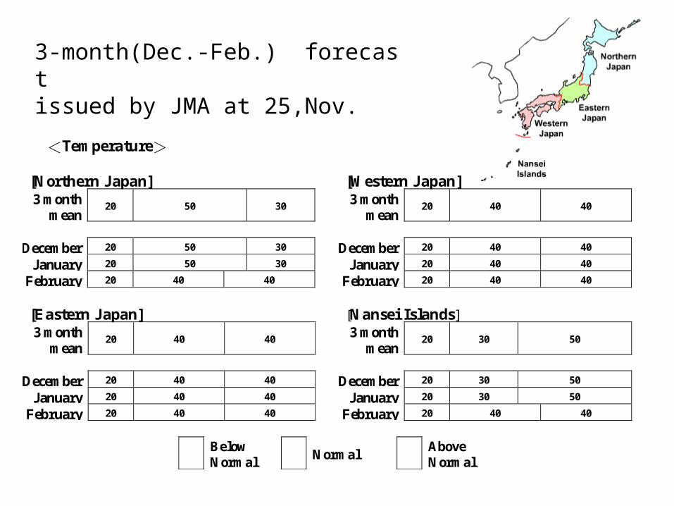
＜Temperature＞

[Northern J apan]3 month

mean20 50 30

December 20 50 30

January 20 50 30

February 20 40 40

[Eastern J apan]3 month

mean20 40 40

December 20 40 40

January 20 40 40

February 20 40 40

[Western J apan]3 month

mean20 40 40

December 20 40 40

January 20 40 40

February 20 40 40

[Nansei Islands]3 month

mean20 30 50

December 20 30 50

January 20 30 50

February 20 40 40

BelowNormal

NormalAboveNormal

3-month(Dec.-Feb.) forecastissued by JMA at 25,Nov.

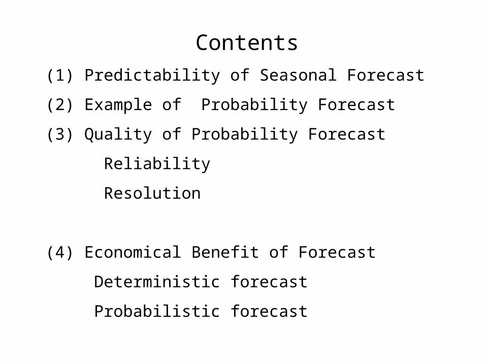
Contents

(1) Predictability of Seasonal Forecast

(2) Example of Probability Forecast

(3) Quality of Probability Forecast

Reliability

Resolution

(4) Economical Benefit of Forecast

Deterministic forecast

Probabilistic forecast

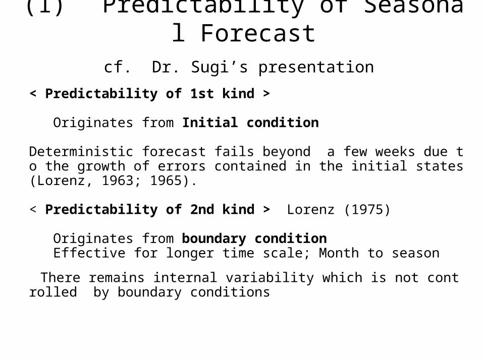
(1) 　 Predictability of Seasonal Forecastcf. Dr. Sugi’s presentation

< Predictability of 1st kind >

Originates from Initial condition Deterministic forecast fails beyond a few weeks due to the growth of errors contained in the initial states (Lorenz, 1963; 1965).

< Predictability of 2nd kind > Lorenz (1975)

Originates from boundary condition Effective for longer time scale; Month to season There remains internal variability which is not controlled by boundary conditions

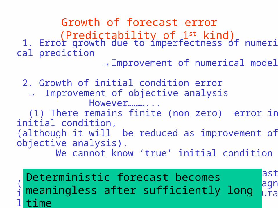
Growth of forecast error 　 (Predictability of 1st kind)

1. Error growth due to imperfectness of numerical prediction ⇒Improvement of numerical model

2. Growth of initial condition error　⇒ Improvement of objective analysis However………... 　　 (1) There remains finite (non zero) error in initial condition,(although it will be reduced as improvement of objective analysis). We cannot know ‘true’ initial condition

　 (2)Small initial error(difference) grows fast(exponentially) as time progresses and the magnitude of error becomes the same order as natural variability after a certain time. ⇒Chaos

Deterministic forecast becomes meaningless after sufficiently long time

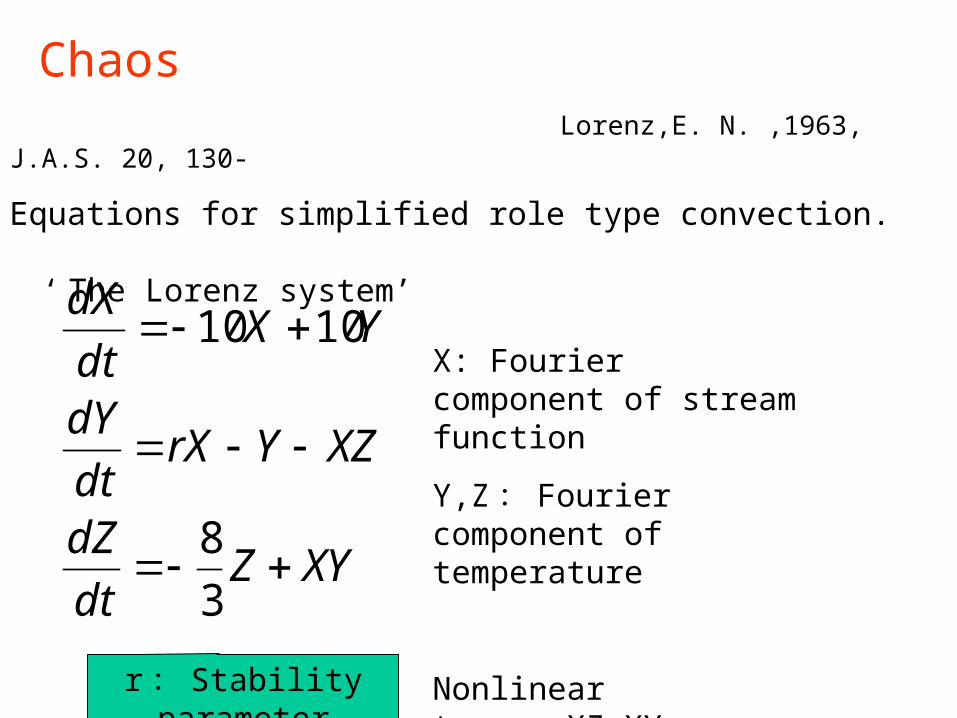
Chaos 　

　　　　　　　　　　　　　　　　　 Lorenz,E. N. ,1963, J.A.S. 20, 130-

Equations for simplified role type convection. 　　　　　　　　　　　　　　　　　　　　　　　　　　　　　　　‘ The Lorenz system’ 　

XYZdt

dZ

XZYrXdt

dY

YXdt

dX

3

8

1010X: Fourier component of stream function

Y,Z ： Fourier component of temperature

Nonlinear terms :XZ,XY

r ： Stability parameter

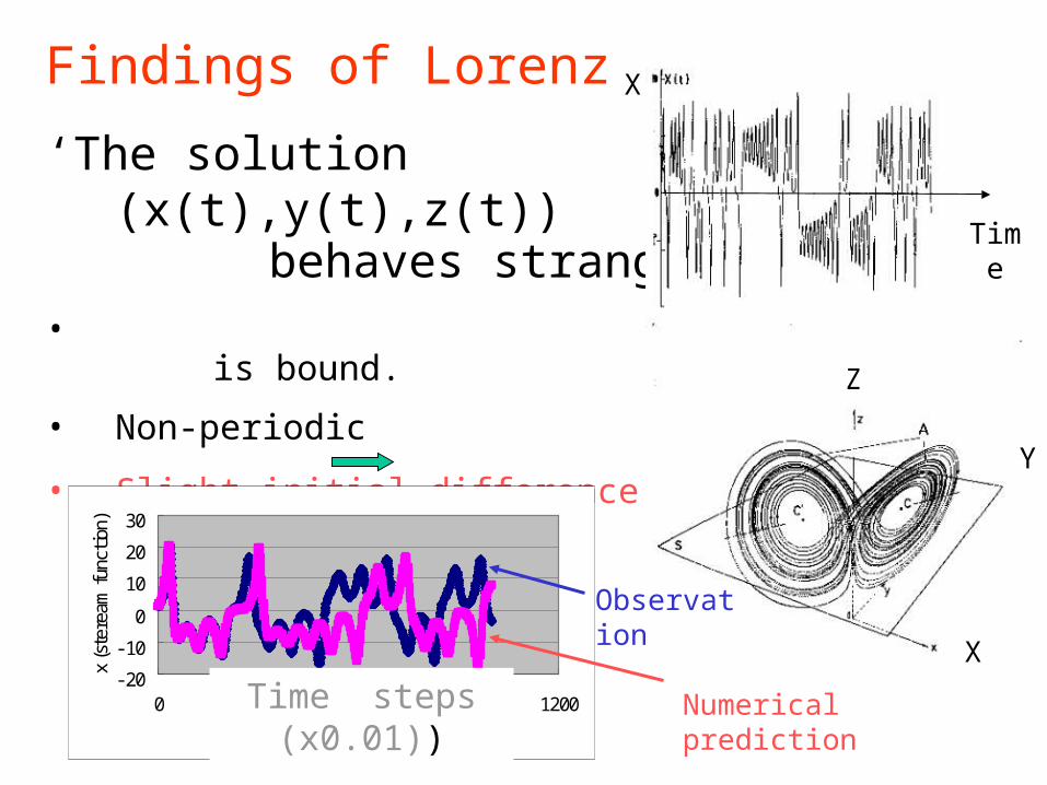
Findings of Lorenz

‘The solution (x(t),y(t),z(t)) behaves strangely’　•

The solution (x(t),y(t),z(t))

is bound.

• Non-periodic

• Slight initial difference causes large difference. Chaos

　

-20

-10

0

10

20

30

0 200 400 600 800 1000 1200

time steps (x0.01)

x (s

tere

am fu

nctio

n)

Time

X

X

Y

Z

Time steps (x0.01))

Numerical prediction

Observation

What can we do on the predictability limit?

Predictability limit varies depending on flow pattern.

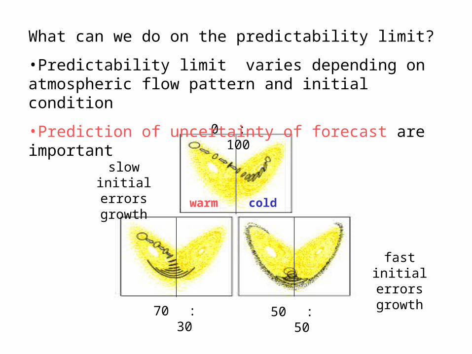
slow initial errors growth

fast initial errors growth

0 　 : 　 100

70 　 : 　30

50 　 : 　50

What can we do on the predictability limit?

•Predictability limit varies depending on atmospheric flow pattern and initial condition

•Prediction of uncertainty of forecast are important

warm cold

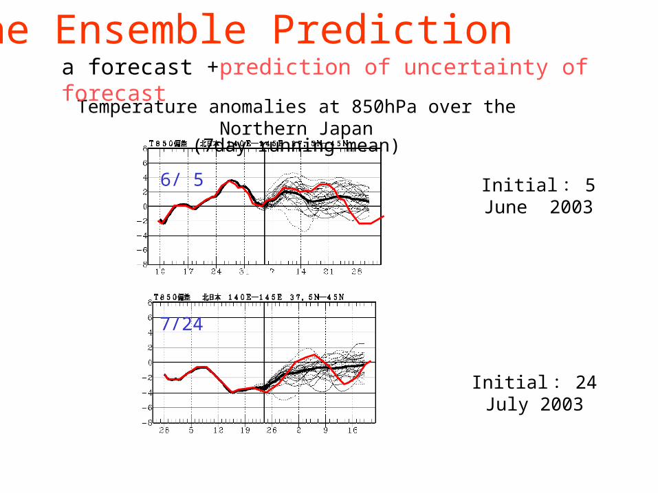
Initial ： 24 July 2003

Initial ： 5 June 2003

Temperature anomalies at 850hPa over the Northern Japan(7day running mean)

The Ensemble Prediction

6/ 5

7/24

a forecast +prediction of uncertainty of forecast

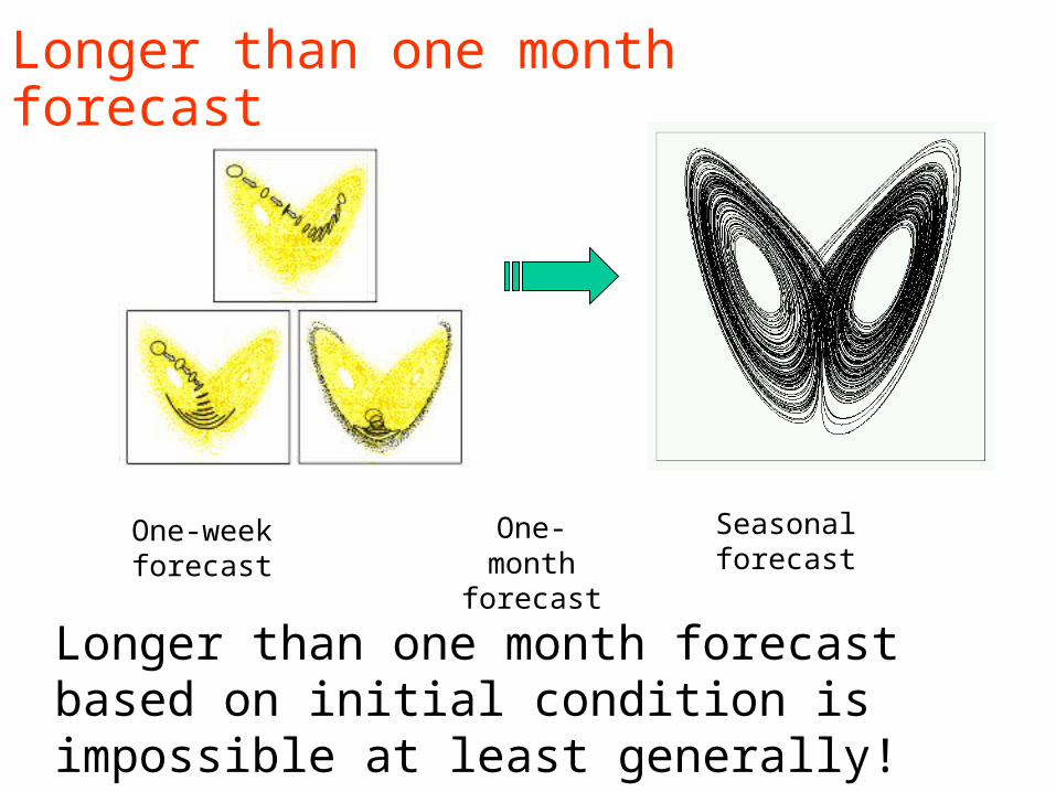
Longer than one month forecast

One-week forecast

One-month forecast

Seasonal forecast

Longer than one month forecast based on initial condition is impossible at least generally!

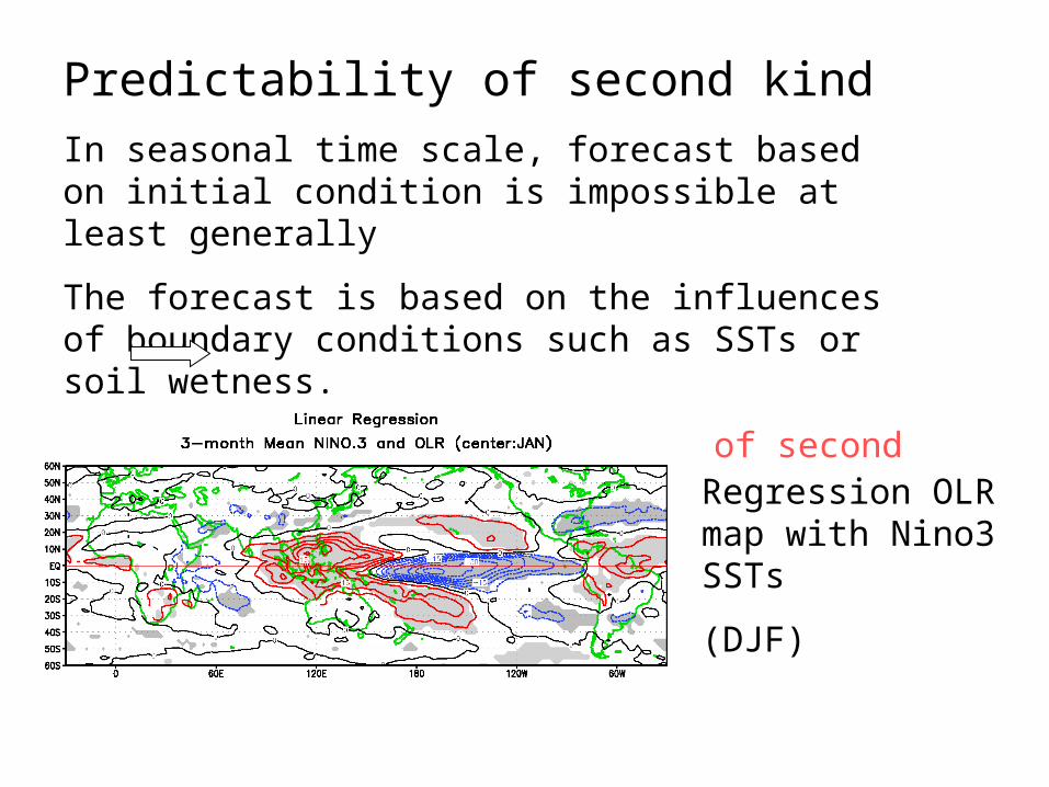
Predictability of second kind

In seasonal time scale, forecast based on initial condition is impossible at least generally

The forecast is based on the influences of boundary conditions such as SSTs or soil wetness.

Prediction of second kind

However ………..

Regression OLR map with Nino3 SSTs

(DJF)

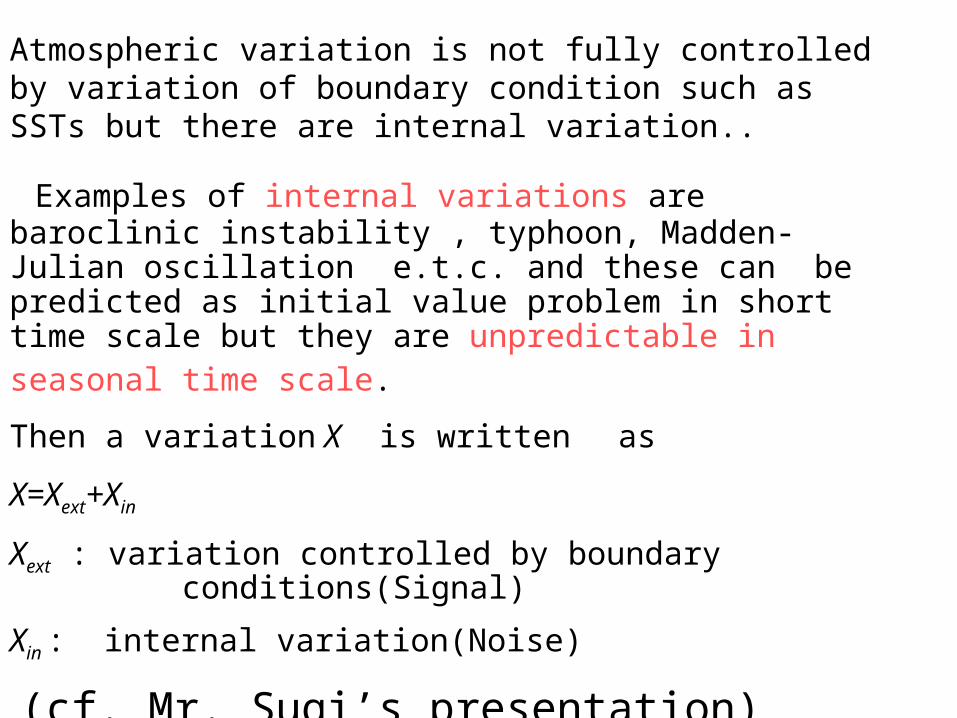
Atmospheric variation is not fully controlled by variation of boundary condition such as SSTs but there are internal variation..

Examples of internal variations are baroclinic instability , typhoon, Madden-Julian oscillation e.t.c. and these can be predicted as initial value problem in short time scale but they are unpredictable in seasonal time scale. Then a variation X is written 　 as

X=Xext+Xin

Xext : variation controlled by boundary conditions(Signal)

Xin : internal variation(Noise)

(cf. Mr. Sugi’s presentation)

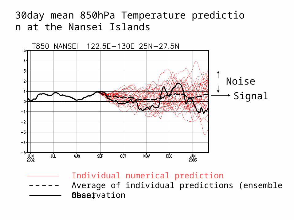
Individual numerical predictionAverage of individual predictions (ensemble mean)Observation

30day mean 850hPa Temperature prediction at the Nansei Islands

Signal

Noise

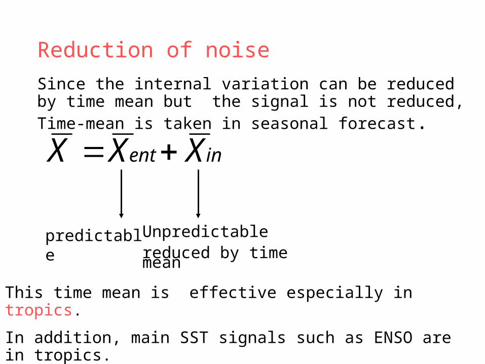
Reduction of noise

Since the internal variation can be reduced by time mean but the signal is not reduced, Time-mean is taken in seasonal forecast.

inent XXX

predictable Unpredictable reduced by time mean

This time mean is effective especially in tropics.

In addition, main SST signals such as ENSO are in tropics.

Seasonal forecast in tropics is easier than in mid-latitude.

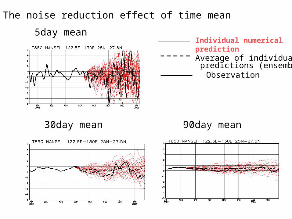
The noise reduction effect of time mean

5day mean

30day mean 90day mean

Individual numericalpredictionAverage of individual predictions (ensemble mean)

Observation

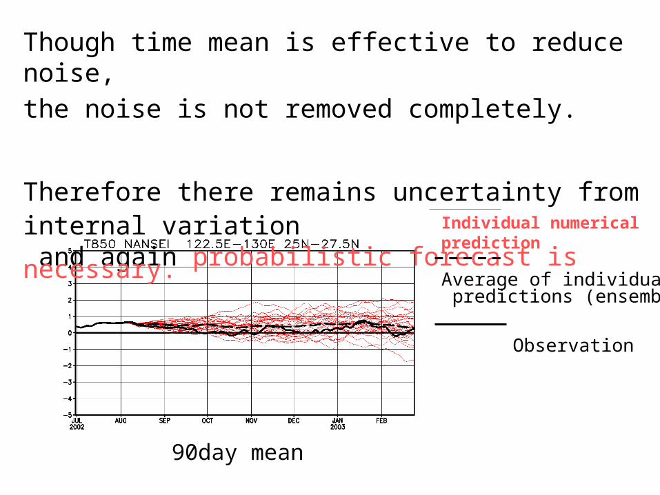
Though time mean is effective to reduce noise,

the noise is not removed completely.

Therefore there remains uncertainty from internal variation and again probabilistic forecast is necessary.

90day mean

Individual numericalprediction

Average of individual predictions (ensemble mean)

Observation

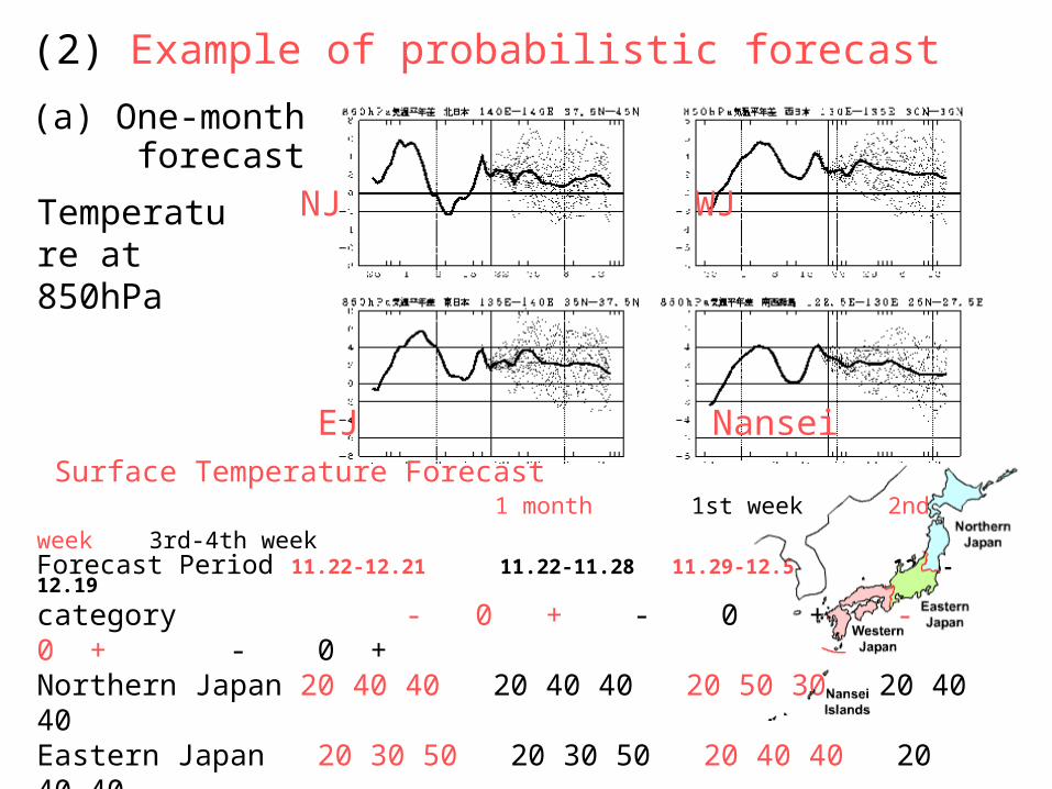
(2) Example of probabilistic forecast

(a) One-month forecast

Surface Temperature Forecast 1 month 1st week 2nd week 3rd-4th week Forecast Period 11.22-12.21 11.22-11.28 11.29-12.5 12.6-12.19

category - 0 + - 0 + - 0 + - 0 + Northern Japan 20 40 40 20 40 40 20 50 30 20 40 40 Eastern Japan 20 30 50 20 30 50 20 40 40 20 40 40 Western Japan 10 40 50 10 40 50 20 30 50 20 40 40 Nansei Islands 10 40 50 10 30 60 20 30 50 20 40 40 ( category : below normal, 0 : near normal, + : above normal, Unit : %)

NJ

EJ

WJ

Nansei

Temperature at 850hPa

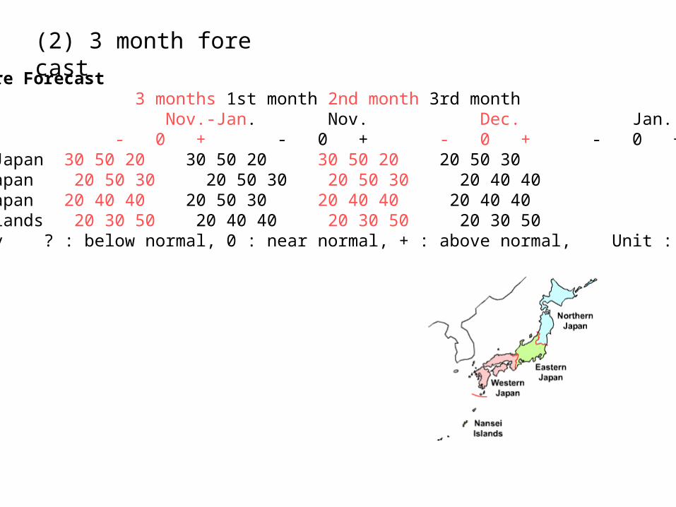
(2) 3 month forecast

Temperature Forecast Period 3 months 1st month 2nd month 3rd month Nov.-Jan. Nov. Dec. Jan. Category - 0 + - 0 + - 0 + - 0 + Northern Japan 30 50 20 30 50 20 30 50 20 20 50 30 Eastern Japan 20 50 30 20 50 30 20 50 30 20 40 40 Western Japan 20 40 40 20 50 30 20 40 40 20 40 40 Nansei Islands 20 30 50 20 40 40 20 30 50 20 30 50 ( category ? : below normal, 0 : near normal, + : above normal, Unit : %)

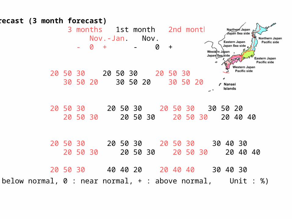
Precipitation Forecast (3 month forecast) Period 3 months 1st month 2nd month 3rd month Nov.-Jan. Nov. Dec. Jan. category - 0 + - 0 + - 0 + - 0 +

Northern Japan Japan Sea side 20 50 30 20 50 30 20 50 30 30 40 30 Pacific side 30 50 20 30 50 20 30 50 20 30 40 30 Eastern Japan Japan Sea side 20 50 30 20 50 30 20 50 30 30 50 20 Pacific side 20 50 30 20 50 30 20 50 30 20 40 40

Western Japan Japan Sea side 20 50 30 20 50 30 20 50 30 30 40 30 Pacific side 20 50 30 20 50 30 20 50 30 20 40 40

Nansei Islands 20 50 30 40 40 20 20 40 40 30 40 30

( category -: below normal, 0 : near normal, + : above normal, Unit : %)

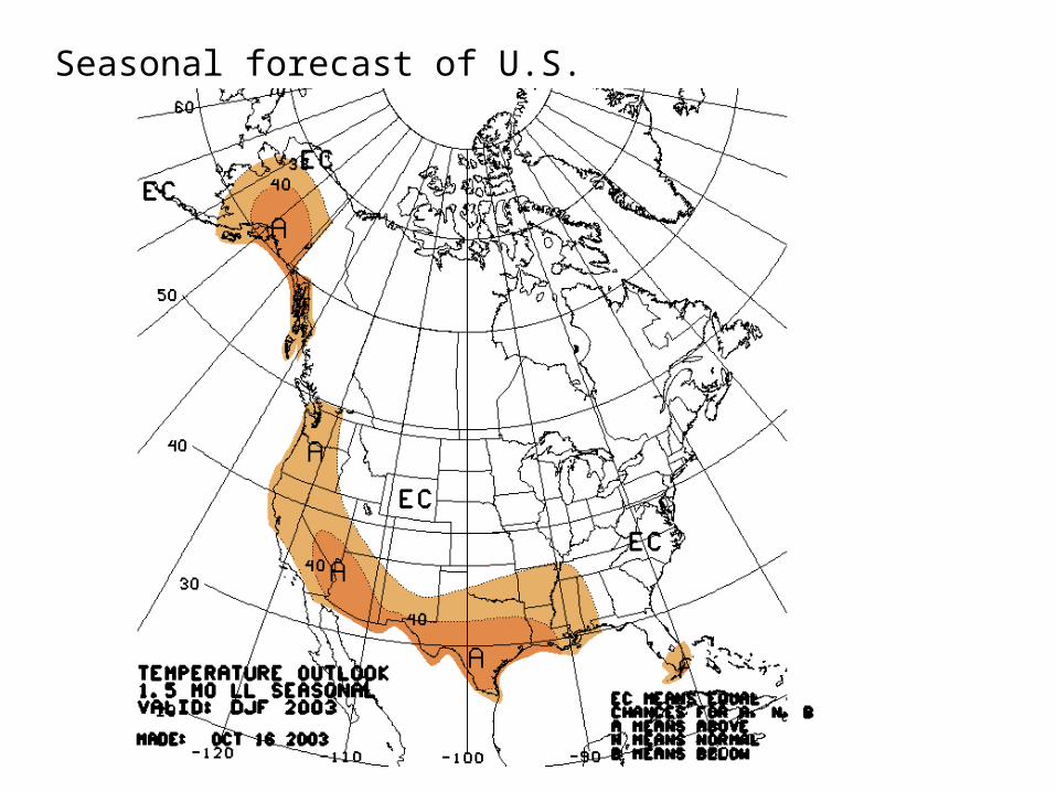
Seasonal forecast of U.S.

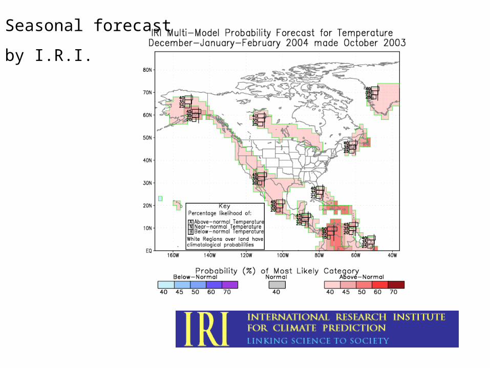
Seasonal forecast

by I.R.I.

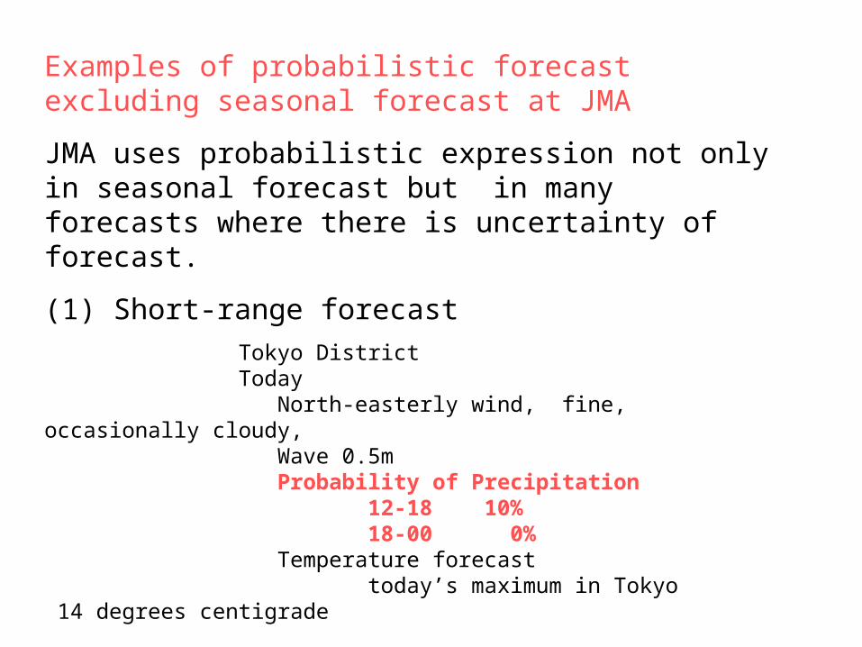
Examples of probabilistic forecast excluding seasonal forecast at JMA

JMA uses probabilistic expression not only in seasonal forecast but in many forecasts where there is uncertainty of forecast.

(1) Short-range forecast

Tokyo District Today North-easterly wind, fine, occasionally cloudy, Wave 0.5m Probability of Precipitation 12-18 10% 18-00 0% Temperature forecast today’s maximum in Tokyo 14 degrees centigrade

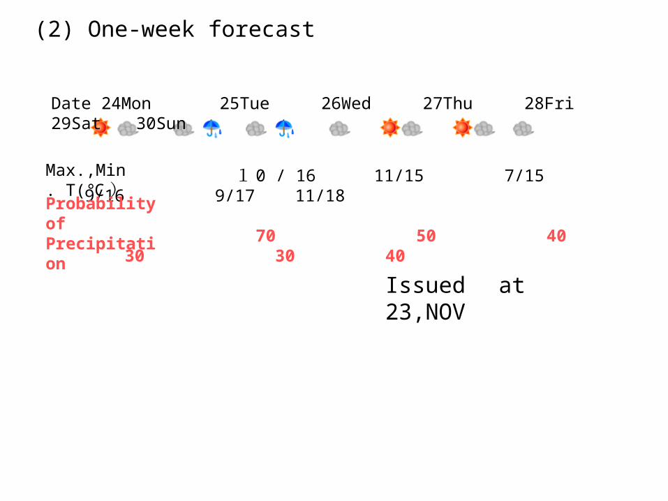
　　　　　　　　　１ 0 / 16 　　　 11/15 7/15 9/16 9/17 11/18 　　　　　　　　　　 70 50 40 30 30 40

Date 24Mon 　　　 25Tue 　　 26Wed 　　 27Thu 　　 28Fri 　　 29Sat 　30Sun

Max.,Min. T(℃ ）Probability of Precipitation

(2) One-week forecast

Issued 　 at 　23,NOV 　

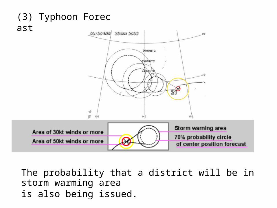
(3) Typhoon Forecast

The probability that a district will be in storm warming area is also being issued.

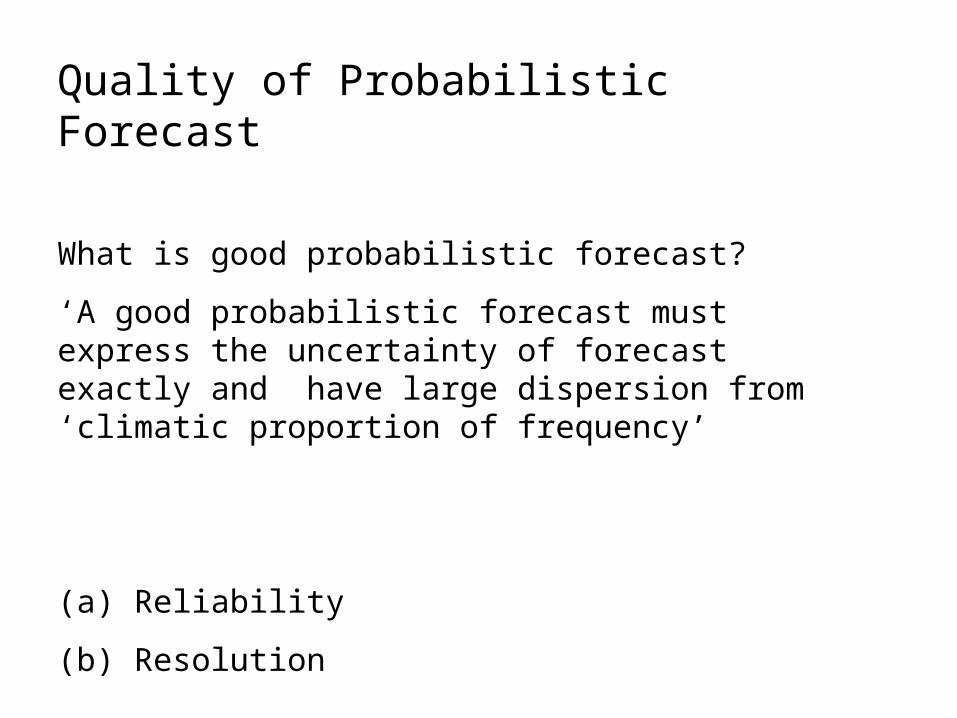
Quality of Probabilistic Forecast

What is good probabilistic forecast?

‘A good probabilistic forecast must express the uncertainty of forecast exactly and have large dispersion from ‘climatic proportion of frequency’

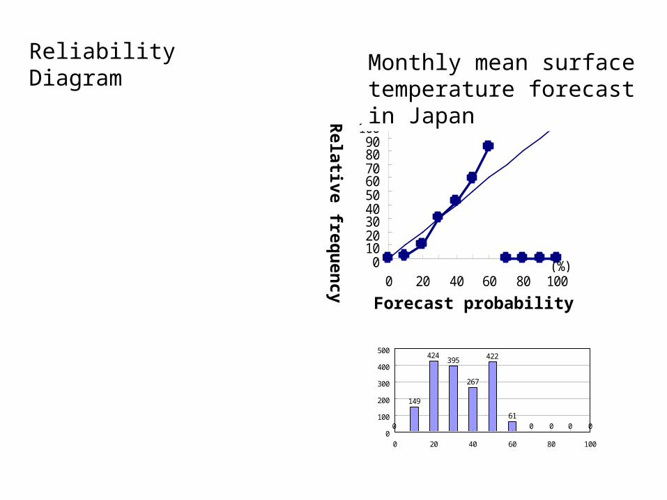
(a) Reliability

(b) Resolution

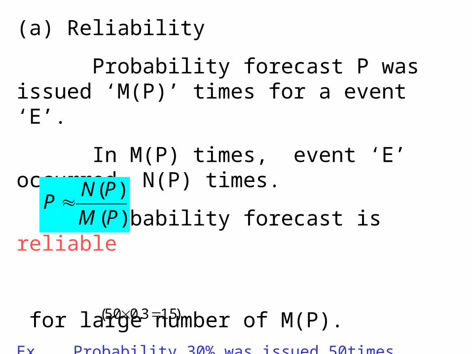
(a) Reliability

Probability forecast P was issued ‘M(P)’ times for a event ‘E’.

In M(P) times, event ‘E’ occurred N(P) times.

If probability forecast is reliable

for large number of M(P).

Ex. Probability 30% was issued 50times. Event ‘E’ is expected to occur about 15times in them.

)(

)(

PM

PNP

)153.050(

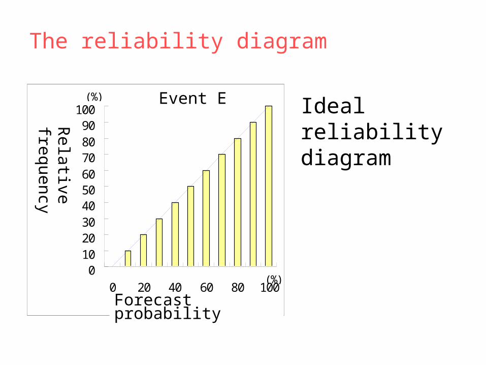
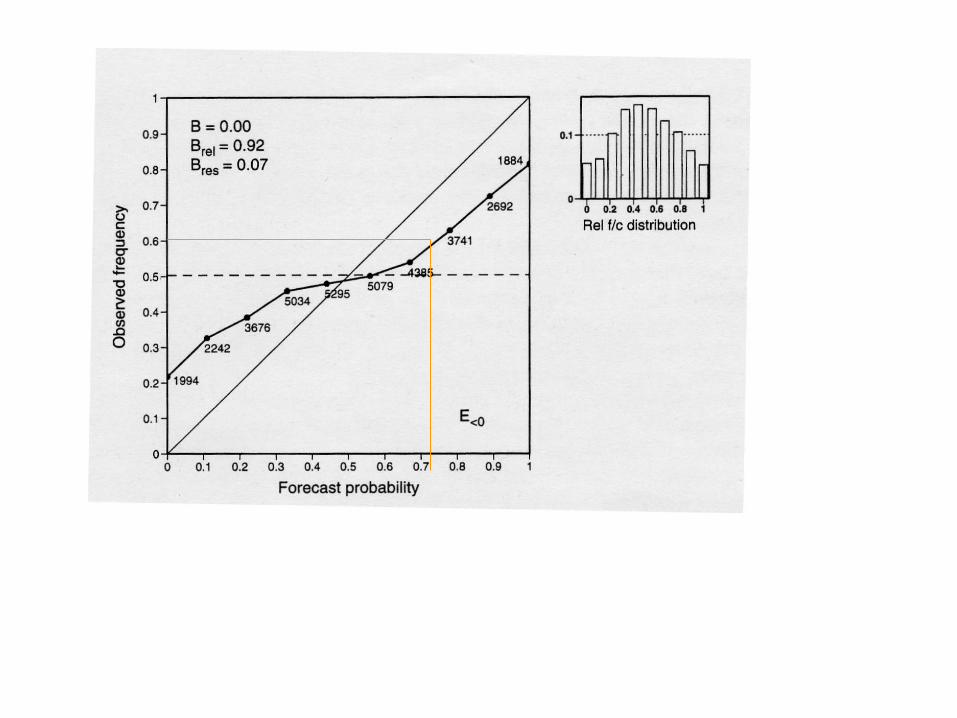
The reliability diagram

平均気温

0102030405060708090

100

0 20 40 60 80 100(%)

(%)

予報確率

確率値別出現率

Event E

Relative frequency

Forecast probability

Ideal reliability diagram

平均気温（発表予報）

0102030405060708090

100

0 20 40 60 80 100(%)

(%)

0

149

424395

267

422

610 0 0 0

0

100

200

300

400

500

0 20 40 60 80 100

Reliability Diagram Monthly mean surface temperature forecast in Japan

Relative frequency

Forecast probability

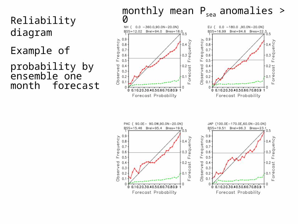
Reliability diagram

Example of

probability by ensemble one month forecast

monthly mean Psea anomalies >0

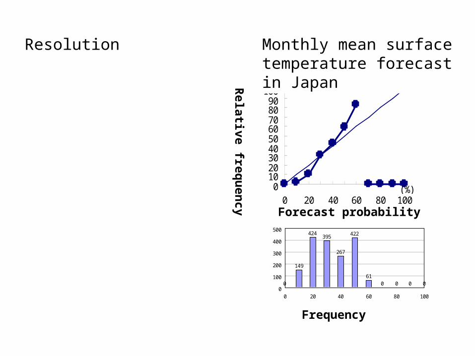
(b) Resolution

Climatorogical relative frequency for a event is perfectly reliableso far as there is no climatic Change.

ex. It is known that relative frequency of rainy day is about 30% at Tokyo from historical data set.

Can we issue probability of 30% as a tomorrow's probability of precipitation at Tokyo every day?

When the reliability is perfect, dispersion of probability from climatorogical relative frequency is another measure of probabilistic forecast quality ‘resolution’.

The best resolution probabilistic forecasts are those of 100% or 0%

provided that reliability is perfect. =perfect forecast.

平均気温（発表予報）

0102030405060708090

100

0 20 40 60 80 100(%)

(%)

平均気温（発表予報）

0102030405060708090

100

0 20 40 60 80 100(%)

(%)

0

149

424395

267

422

610 0 0 0

0

100

200

300

400

500

0 20 40 60 80 100

Monthly mean surface temperature forecast in Japan

Relative frequency

Forecast probability

Frequency

Resolution

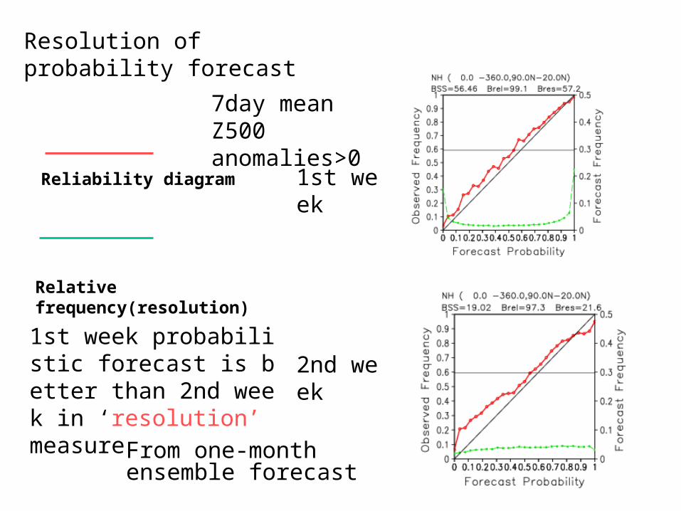
Resolution of probability forecast

1st week

2nd week

Reliability diagram

Relative frequency(resolution)

1st week probabilistic forecast is better than 2nd week in ‘resolution’ measure

7day mean Z500 anomalies>0

From one-month ensemble forecast

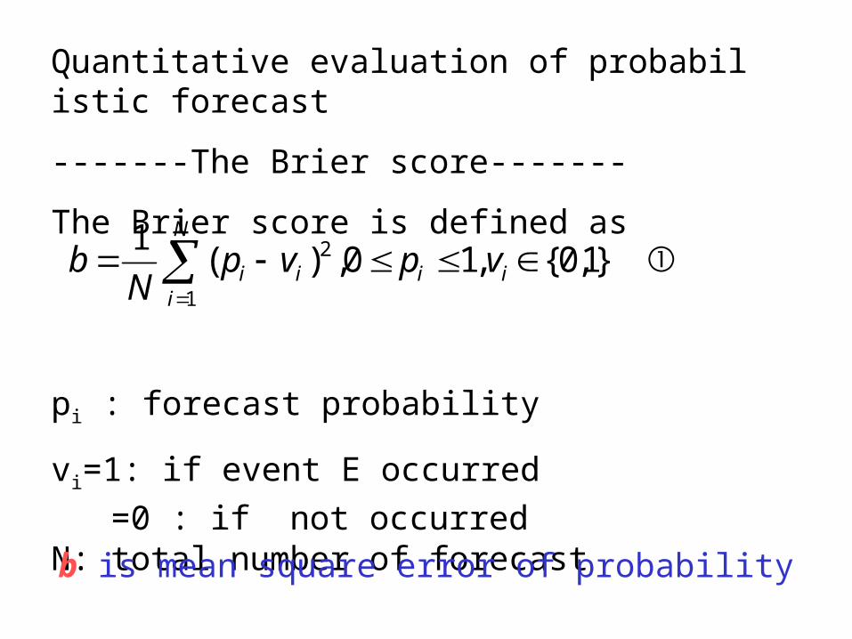
Quantitative evaluation of probabilistic forecast

-------The Brier score-------

The Brier score is defined as

pi : forecast probability

vi=1: if event E occurred

=0 : if not occurred N: total number of forecast

①}1,0{,10,)(1 2

1

iii

N

ii vpvp

Nb

b is mean square error of probability

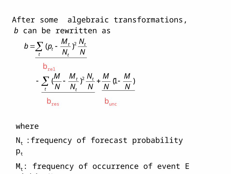
After some algebraic transformations,

b can be rewritten as

)1()(

)(

2

2

N

M

N

M

N

N

N

M

N

M

N

N

N

Mpb

t

t

t

t

t

t

t

tt

where

Nt :frequency of forecast probability pt

Mt: frequency of occurrence of event E within Nt

brel

bres bunc

N

N

N

Mpb t

t t

ttrel

2)(

N

N

N

M

N

Mb t

t

t

tres

2)(

)1(N

M

N

Mbunc

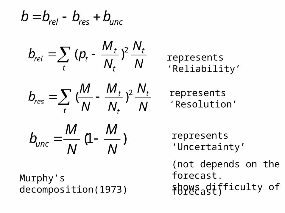
uncresrel bbbb

represents ‘Reliability’

represents ‘Resolution’

represents ‘Uncertainty’

(not depends on the forecast.shows difficulty of forecast)

Murphy’s decomposition(1973)

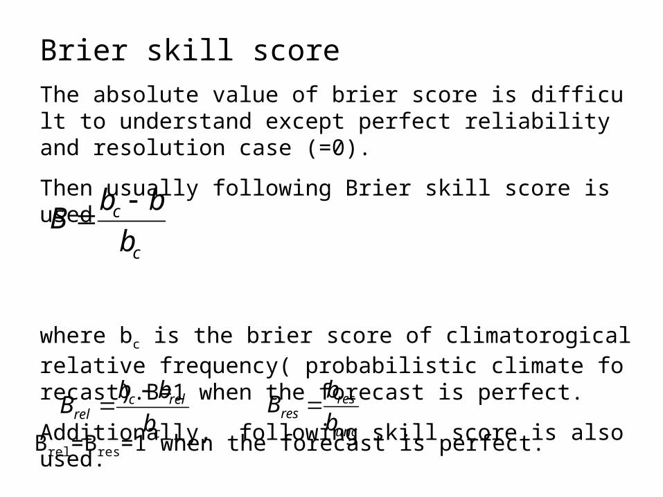
Brier skill score

The absolute value of brier score is difficult to understand except perfect reliability and resolution case (=0).

Then usually following Brier skill score is used

where bc is the brier score of climatorogical relative frequency( probabilistic climate forecast).B=1 when the forecast is perfect.

Additionally, following skill score is also used.

c

c

b

bbB

c

relcrel b

bbB

unc

resres b

bB

Brel=Bres=1 when the forecast is perfect.

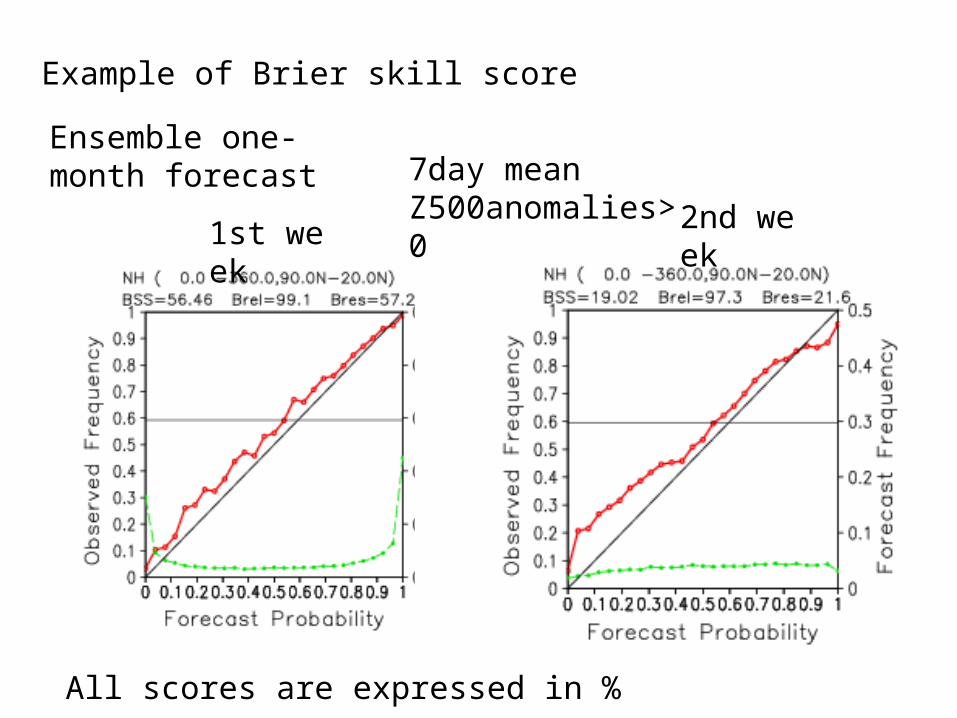
Example of Brier skill score

1st week 2nd week

7day mean Z500anomalies>0

Ensemble one-month forecast

All scores are expressed in %

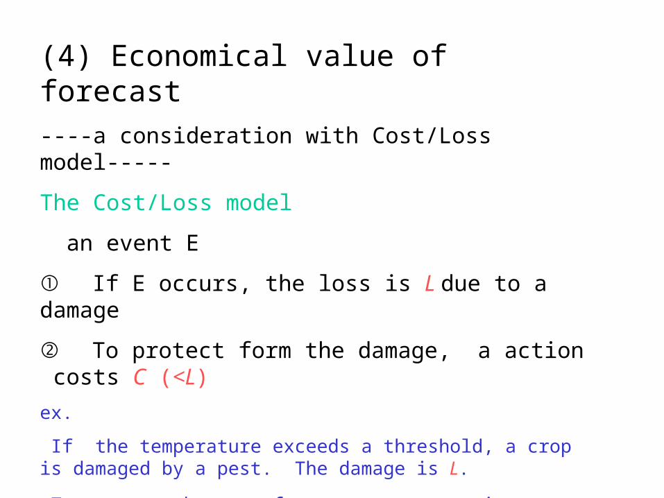
(4) Economical value of forecast

----a consideration with Cost/Loss model-----

The Cost/Loss model

an event E

① 　 If E occurs, the loss is L due to a damage

② 　 To protect form the damage, a action costs C (<L)

ex.

If the temperature exceeds a threshold, a crop is damaged by a pest. The damage is L.

To protect the crop from a pest , spraying agrochemical is necessary and

it costs C.

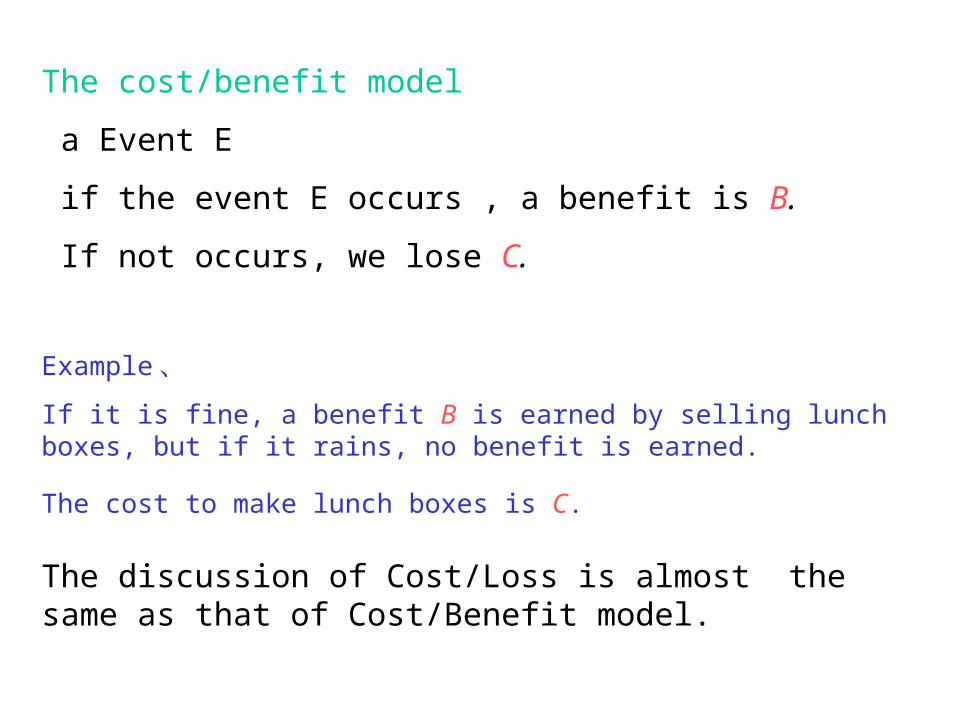
The cost/benefit model

a Event E

if the event E occurs , a benefit is B.

If not occurs, we lose C.

Example 、

If it is fine, a benefit B is earned by selling lunch boxes, but if it rains, no benefit is earned.

The cost to make lunch boxes is C. 　

The discussion of Cost/Loss is almost the same as that of Cost/Benefit model.

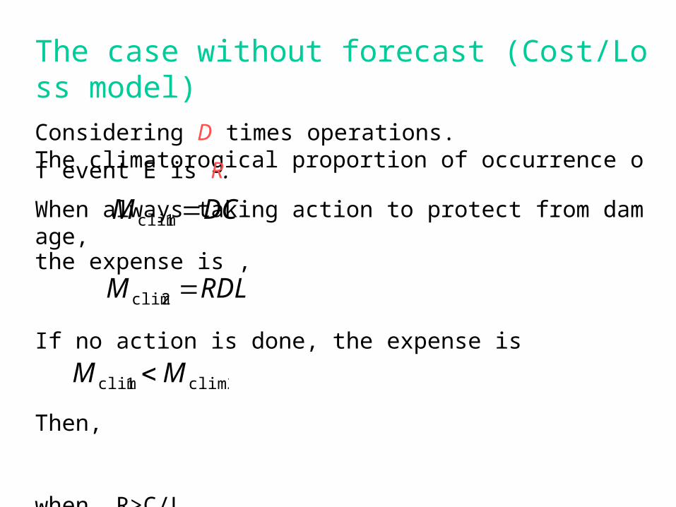
The case without forecast (Cost/Loss model)

Considering D times operations.The climatorogical proportion of occurrence of event E is R.

When always taking action to protect from damage,the expense is ,

If no action is done, the expense is

Then,

when R>C/L

If the event E occurs frequently, it is better to take action always.

DCM 1clim

RDLM 2clim

clim21clim MM

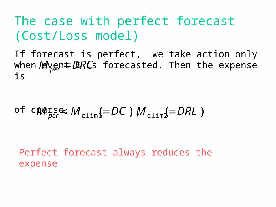
The case with perfect forecast (Cost/Loss model)

If forecast is perfect, we take action only when event E is forecasted. Then the expense is

of course,

DRCM per

)(),( clim2clim1 DRLMDCMM per

Perfect forecast always reduces the expense

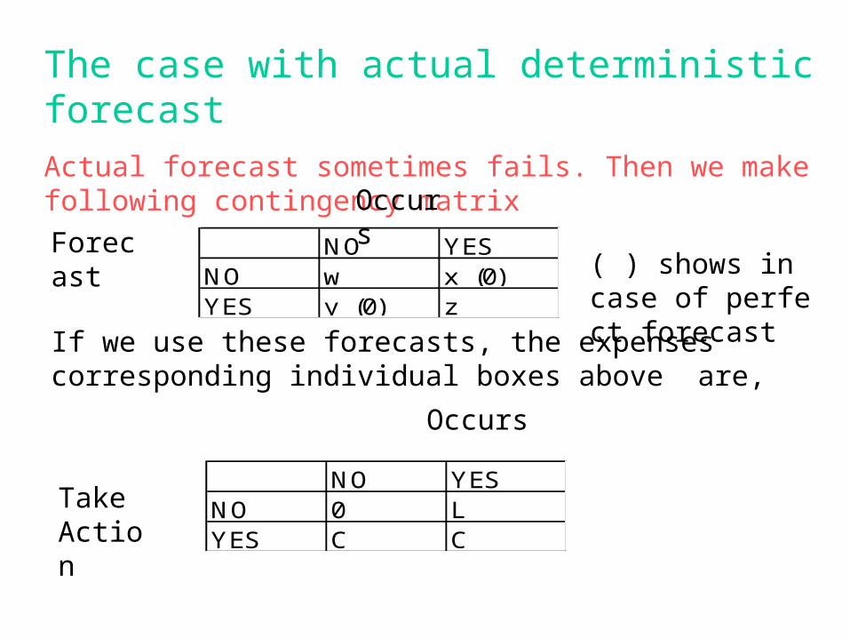
The case with actual deterministic forecast

Actual forecast sometimes fails. Then we make following contingency matrix

NO YES

NO w x (0)YES y (0) z

Forecast

NO YESNO 0 LYES C C

Take Action

If we use these forecasts, the expenses corresponding individual boxes above are,

Occurs

Occurs

( ) shows in case of perfect forecast

D

zxR

zyxwD

yw

yF

zx

zH

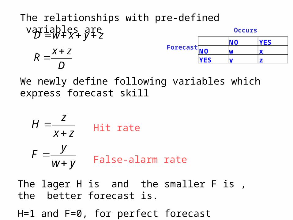
The relationships with pre-defined variables are

We newly define following variables which express forecast skill

Hit rate

False-alarm rate

The lager H is and the smaller F is , the better forecast is.

H=1 and F=0, for perfect forecast

NO YESNO w xYES y z

Forecast

Occurs

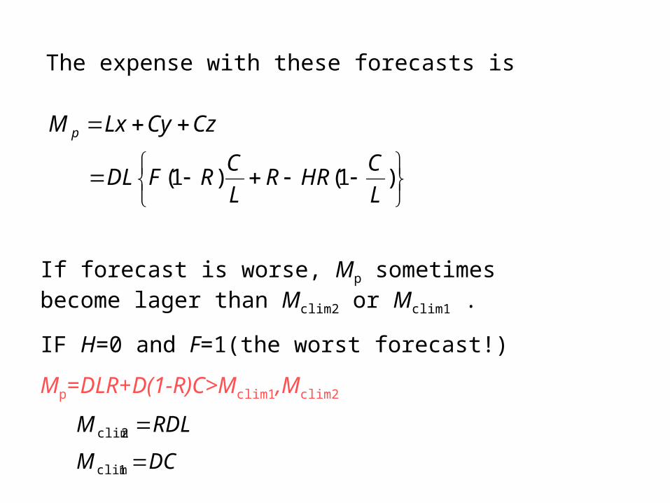
The expense with these forecasts is

)1()1(L

CHRR

L

CRFDL

CzCyLxM p

DCM 1clim

RDLM 2clim

If forecast is worse, Mp sometimes become lager than Mclim2 or Mclim1 .

IF H=0 and F=1(the worst forecast!)

Mp=DLR+D(1-R)C>Mclim1,Mclim2

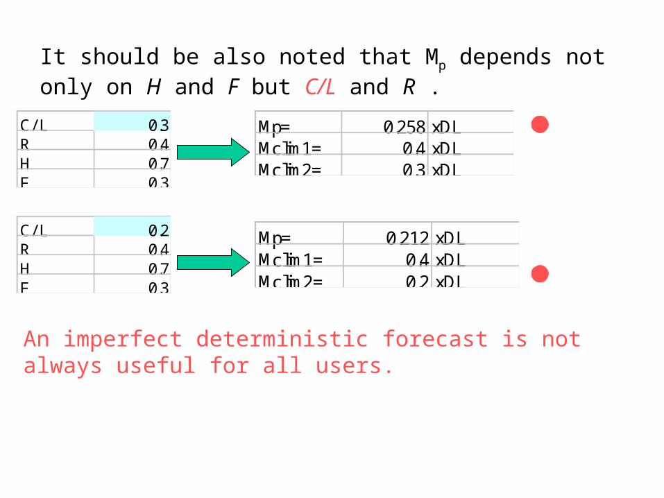
It should be also noted that Mp depends not only on H and F but C/L and R .

C/ L 0.3R 0.4H 0.7F 0.3

Mp= 0.258 xDLMclim1= 0.4 xDLMclim2= 0.3 xDL

C/ L 0.2R 0.4H 0.7F 0.3

Mp= 0.212 xDLMclim1= 0.4 xDLMclim2= 0.2 xDL

An imperfect deterministic forecast is not always useful for all users.

The case with probabilistic forecast (Cost/Loss model)How do we use probabilistic forecast?

Consider to take action always when the probabilistic forecast is P0 for the occurrence of event E. The expense is,

Mp0=DpC

where Dp is total frequency that the event E was forecasted with probability P0

If probabilistic forecast is perfectly reliable, the frequency that event E occurred is DpP0 and then the expense without taking action is

Mc=DpP0L

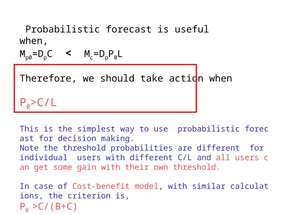
Probabilistic forecast is usefulwhen,Mp0=DpC < Mc=DpP0L

Therefore, we should take action when

P0>C/L

This is the simplest way to use probabilistic forecast for decision making. Note the threshold probabilities are different for individual users with different C/L and all users can get some gain with their own threshold.

In case of Cost-benefit model, with similar calculations, the criterion is,

P0 >C/(B+C)

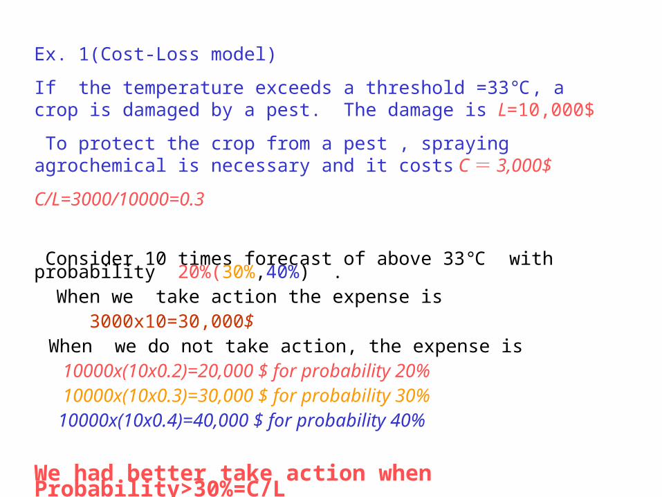
Ex. 1(Cost-Loss model)

If the temperature exceeds a threshold =33 , a crop is damaged by a pest. ℃The damage is L=10,000$

To protect the crop from a pest , spraying agrochemical is necessary and it costs C ＝ 3,000$

C/L=3000/10000=0.3

Consider 10 times forecast of above 33 with probability ℃20%(30%,40%) . When we take action the expense is 3000x10=30,000$ When we do not take action, the expense is 10000x(10x0.2)=20,000 $ for probability 20% 10000x(10x0.3)=30,000 $ for probability 30% 10000x(10x0.4)=40,000 $ for probability 40%

We had better take action when Probability>30%=C/L

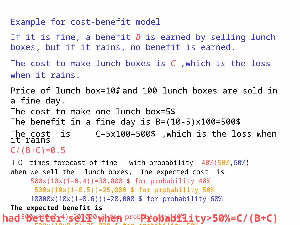
Example for cost-benefit model

If it is fine, a benefit B is earned by selling lunch boxes, but if it rains, no benefit is earned.

The cost to make lunch boxes is C ,which is the loss when it rains.

Price of lunch box=10$ and 100 lunch boxes are sold in a fine day.The cost to make one lunch box=5$The benefit in a fine day is B=(10-5)x100=500$

The cost is C=5x100=500$ ,which is the loss when it rains C/(B+C)=0.5

１０ times forecast of fine with probability 40%(50%,60%)

When we sell the 　 lunch boxes, The expected cost is 500x(10x(1-0.4))=30,000 $ for probability 40% 500x(10x(1-0.5))=25,000 $ for probability 50% 10000x(10x(1-0.6)))=20,000 $ for probability 60%The expected benefit is 500x(10x0.4)=20,000 $ for probability 40% 500x(10x0.5)=25,000 $ for probability 50% 500x(10x0.6)=30,000 $ for probability 60%

　

We had better sell when Probability>50%=C/(B+C)

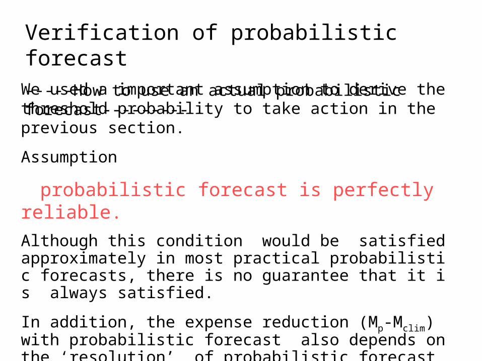
Verification of probabilistic forecast

-----How to use an actual probabilistic forecast---------

We used a important assumption to derive the threshold probability to take action in the previous section.

Assumption

probabilistic forecast is perfectly reliable.

Although this condition would be satisfied approximately in most practical probabilistic forecasts, there is no guarantee that it is always satisfied.

In addition, the expense reduction (Mp-Mclim) with probabilistic forecast also depends on the ‘resolution’ of probabilistic forecast and we cannot know how much it is without verification.

Therefore verification is important to use probabilistic forecast actually.

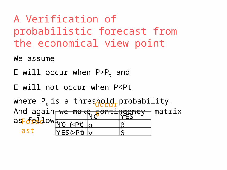
A Verification of probabilistic forecast from the economical view point

We assume

E will occur when P>Pt and

E will not occur when P<Pt

where Pt is a threshold probability. And again we make contingency matrix as follows.

NO YESNO (<Pt) α βYES(>Pt) γ δ

Forecast

Occurs

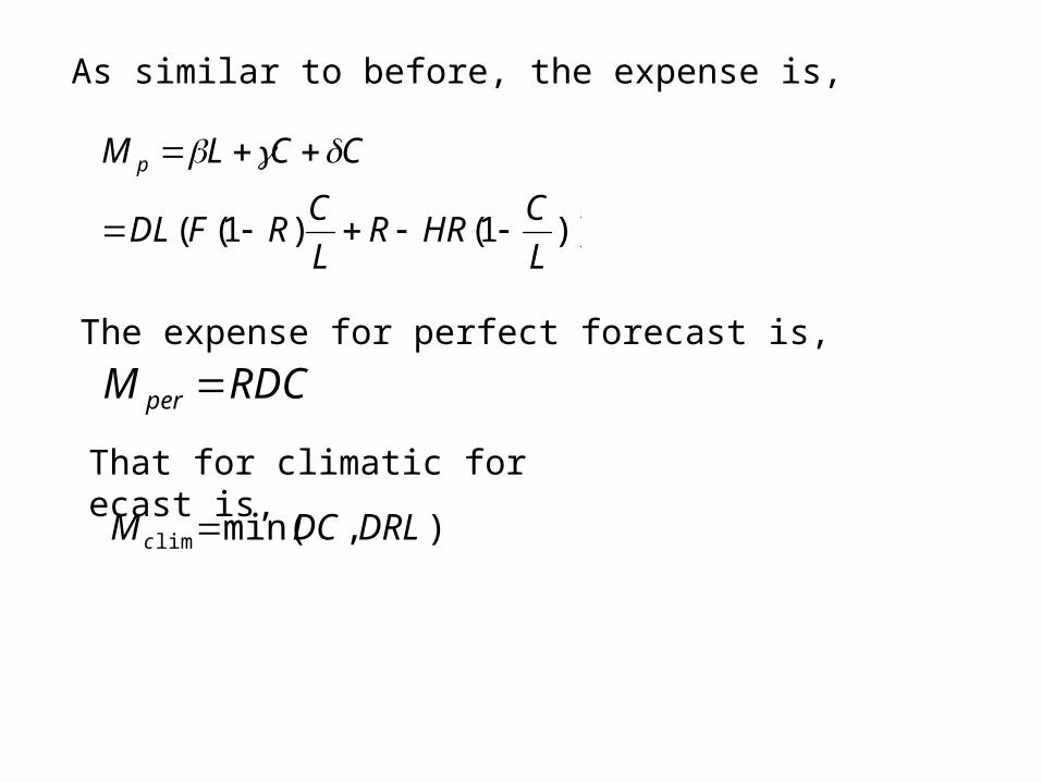
As similar to before, the expense is,

))1()1((

L

CHRR

L

CRFDL

CCLM p

The expense for perfect forecast is,

RDCM per

That for climatic forecast is,

),min(lim DRLDCM c

perc

Pc

MM

MMV

lim

lim

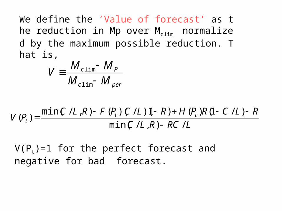
We define the ‘Value of forecast’ as the reduction in Mp over Mclim normalized by the maximum possible reduction. That is,

V(Pt)=1 for the perfect forecast and negative for bad forecast.

LRCRLC

RLCRPHRLCPFRLCPV tt

t /),/min(

)/1()()1)(/)((),/min()(

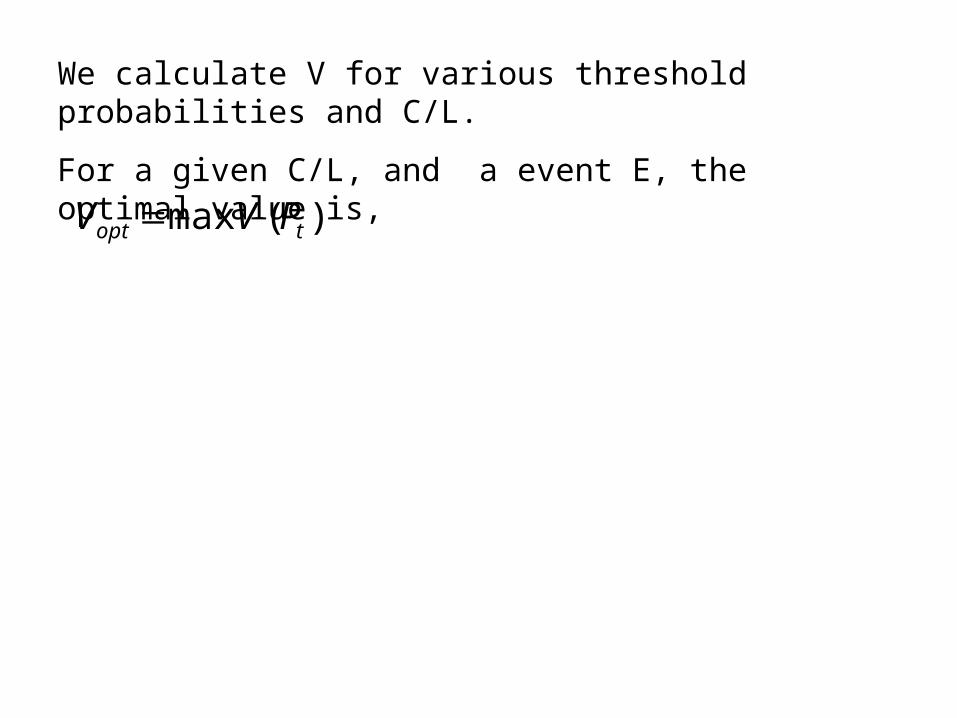
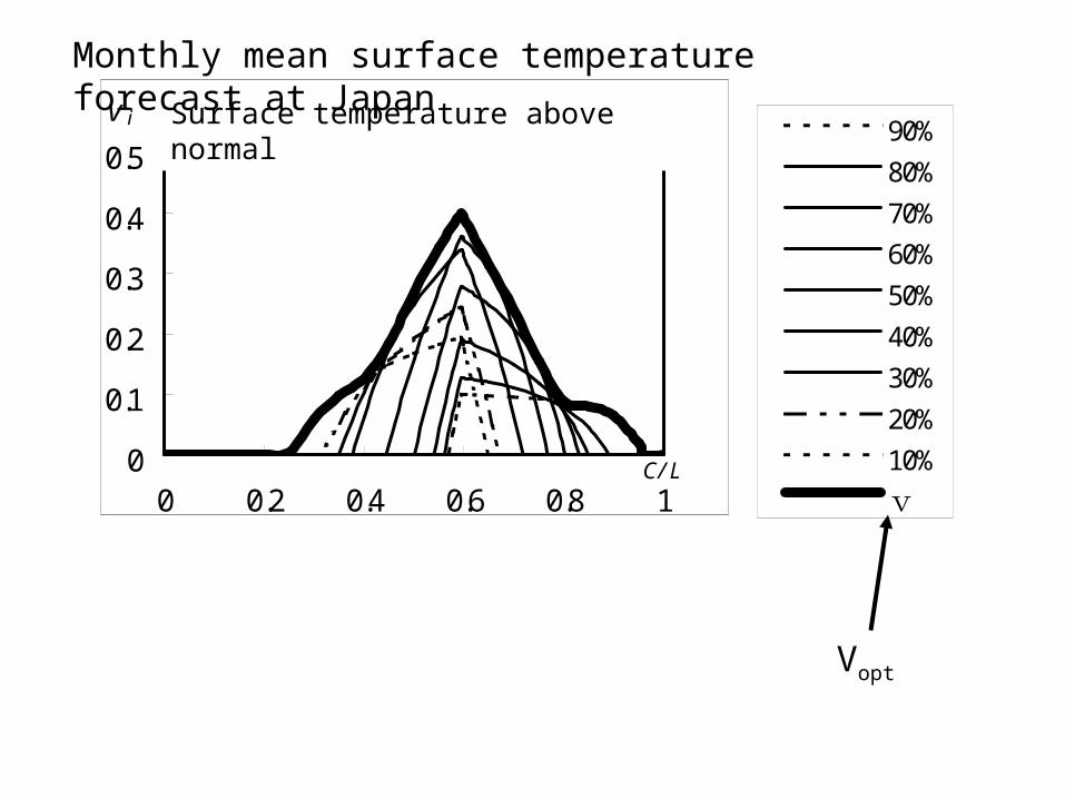
We calculate V for various threshold probabilities and C/L.

For a given C/L, and a event E, the optimal value is,

)(max topt PVV

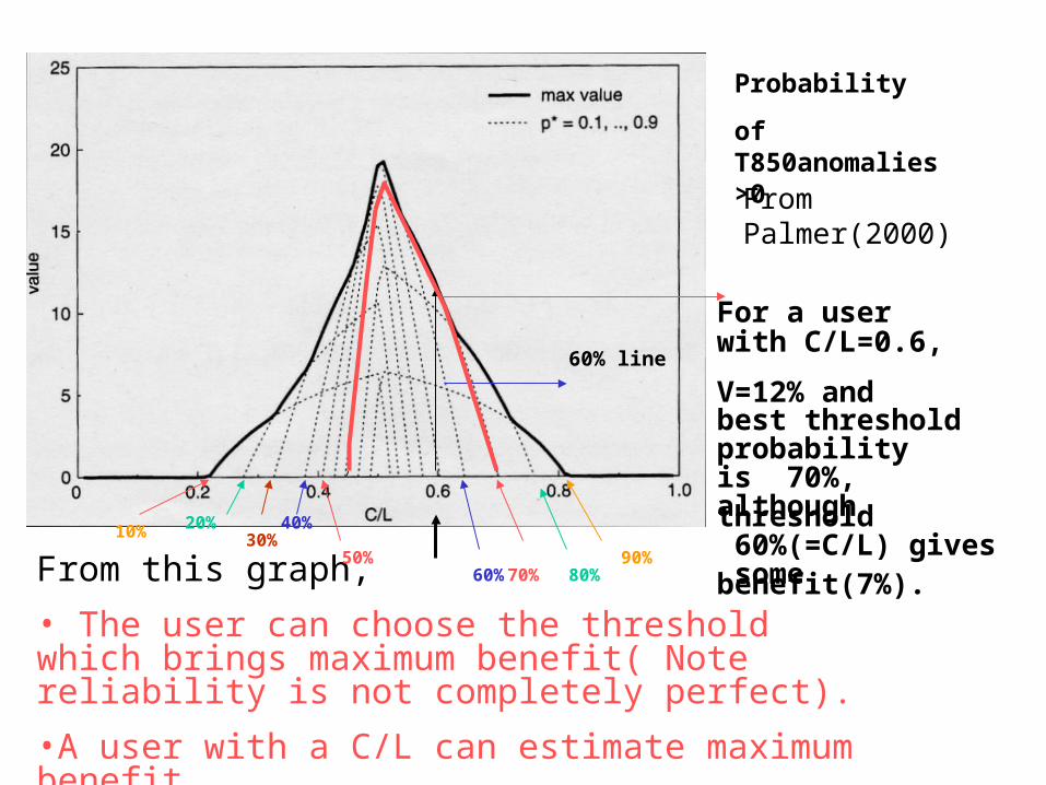
From this graph,

• The user can choose the threshold which brings maximum benefit( Note reliability is not completely perfect).

•A user with a C/L can estimate maximum benefit

Probability

of T850anomalies >0

For a userwith C/L=0.6,

V=12% andbest threshold probabilityis 70%,although threshold 60%(=C/L) gives some benefit(7%).

60% line

90%80%70%60%

40%30%

20%10%

50%

From Palmer(2000)

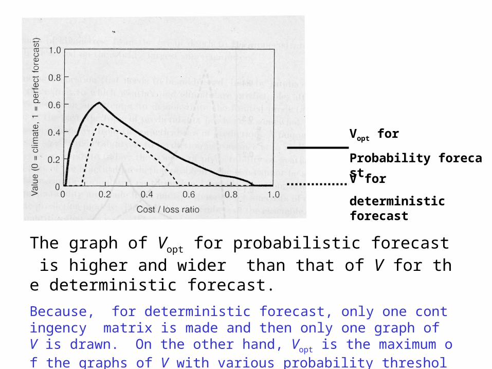
Vopt for

Probability forecast

V for

deterministic forecast

The graph of Vopt for probabilistic forecast is higher and wider than that of V for the deterministic forecast.

Because, for deterministic forecast, only one contingency matrix is made and then only one graph of V is drawn. On the other hand, Vopt is the maximum of the graphs of V with various probability threshold.

確率ガイダンス（気温）1996. 6 1999. 5～

0

20

40

60

80

100

0 20 40 60 80 100

(a)(%)

(%)

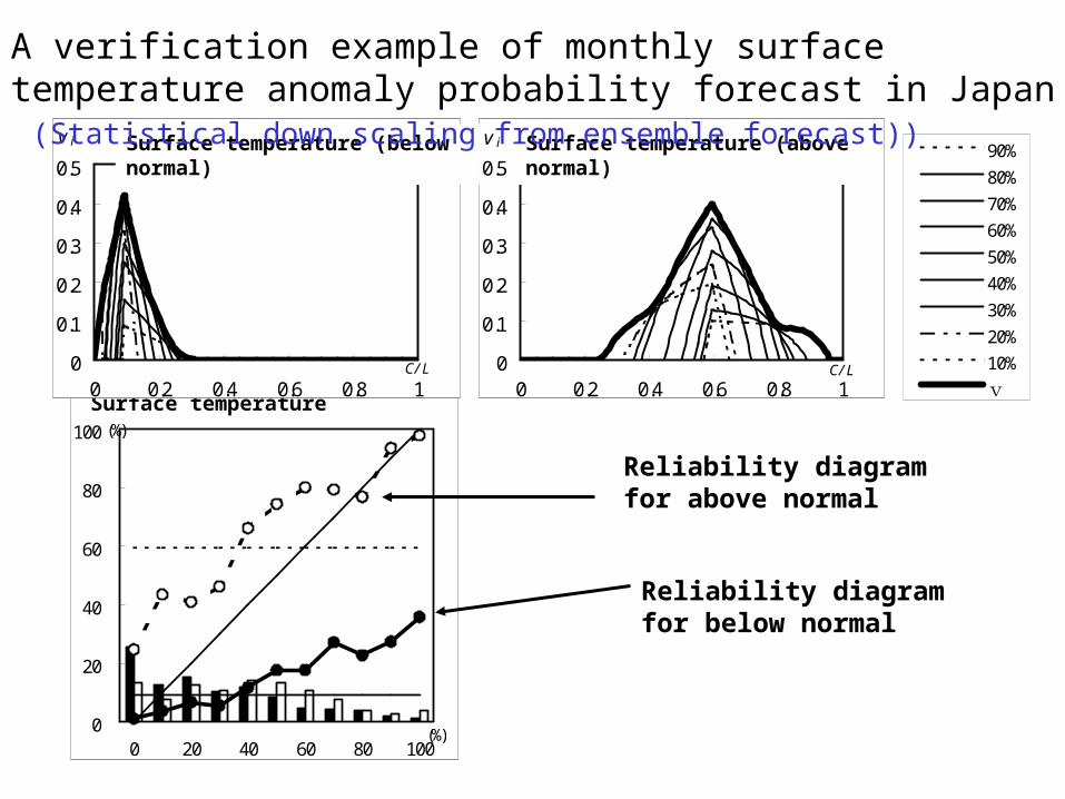
Surface temperature

Reliability diagram for above normal

Reliability diagram for below normal

(b)確率ガイダンス（気温「高い」）

0

0.1

0.2

0.3

0.4

0.5

0 0.2 0.4 0.6 0.8 1

vi

C/ L

0

90%

80%

70%

60%

50%

40%

30%

20%

10%

ｖ

(a)確率ガイダンス（気温「低い」）

0

0.1

0.2

0.3

0.4

0.5

0 0.2 0.4 0.6 0.8 1

vi

C/ L

0

0.1

0.2

0.3

0.4

0.5

0 0.2 0.4 0.6 0.8 1

1

0

0.1

0.2

0.3

0.4

0.5

0 0.2 0.4 0.6 0.8 1

Surface temperature (above normal)Surface temperature (below normal)

A verification example of monthly surface temperature anomaly probability forecast in Japan (Statistical down scaling from ensemble forecast))

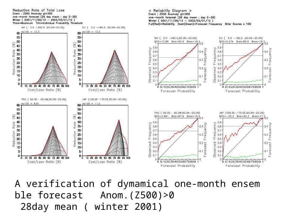
A verification of dymamical one-month ensemble forecast Anom.(Z500)>0 28day mean ( winter 2001)

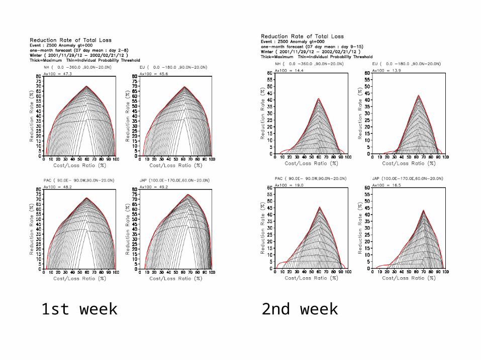
1st week 2nd week

3-4th week

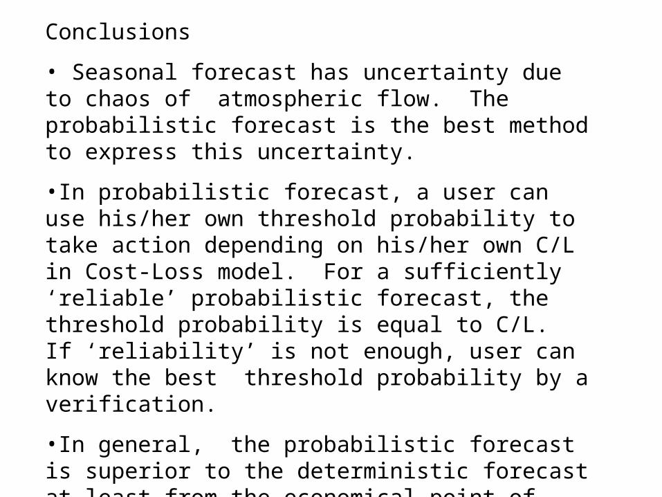
Conclusions

• Seasonal forecast has uncertainty due to chaos of atmospheric flow. The probabilistic forecast is the best method to express this uncertainty.

•In probabilistic forecast, a user can use his/her own threshold probability to take action depending on his/her own C/L in Cost-Loss model. For a sufficiently ‘reliable’ probabilistic forecast, the threshold probability is equal to C/L. If ‘reliability’ is not enough, user can know the best threshold probability by a verification.

•In general, the probabilistic forecast is superior to the deterministic forecast at least from the economical point of view so far as the forecast is not perfect although it seems difficult in some degree. More dissemination of probabilistic forecast is necessary.

Please remember the words ‘uncertainty of forecast’ and ‘cost-loss ratio C/L’.

　

Thank you!

(b)確率ガイダンス（気温「高い」）

0

0.1

0.2

0.3

0.4

0.5

0 0.2 0.4 0.6 0.8 1

vi

C/ L

0

90%

80%

70%

60%

50%

40%

30%

20%

10%

ｖ0

0.1

0.2

0.3

0.4

0.5

0 0.2 0.4 0.6 0.8 1

0

0.1

0.2

0.3

0.4

0.5

0 0.2 0.4 0.6 0.8 1

1

0

0.1

0.2

0.3

0.4

0.5

0 0.2 0.4 0.6 0.8 1

Surface temperature above normal

Monthly mean surface temperature forecast at Japan

Vopt