NBER WORKING PAPER SERIES

PRIVATE RETURNS TO PUBLIC OFFICE

Raymond FismanFlorian Schulz

Vikrant Vig

Working Paper 18095http://www.nber.org/papers/w18095

NATIONAL BUREAU OF ECONOMIC RESEARCH1050 Massachusetts Avenue

Cambridge, MA 02138May 2012

We would like to thank Patrick Bolton, Ben Olken and seminar participants at the LSE-UCL developmentworkshop, Columbia and Warwick University. In addition, Vikrant Vig would like to thank the RAMDresearch grant at the London Business School for their generous support. Kyle Matoba and Jane Zhaoprovided excellent research assistance. The views expressed herein are those of the authors and donot necessarily reflect the views of the National Bureau of Economic Research.

NBER working papers are circulated for discussion and comment purposes. They have not been peer-reviewed or been subject to the review by the NBER Board of Directors that accompanies officialNBER publications.

© 2012 by Raymond Fisman, Florian Schulz, and Vikrant Vig. All rights reserved. Short sectionsof text, not to exceed two paragraphs, may be quoted without explicit permission provided that fullcredit, including © notice, is given to the source.

Private Returns to Public OfficeRaymond Fisman, Florian Schulz, and Vikrant VigNBER Working Paper No. 18095May 2012JEL No. D72,D73,D78

ABSTRACT

We study the wealth accumulation of Indian parliamentarians using public disclosures required ofall candidates since 2003. Annual asset growth of winners is on average 3 to 6 percentage points higherthan runners-up. By performing a within-constituency comparison where both runner-up and winnerrun in consecutive elections, and by looking at the subsample of very close elections, we rule out arange of alternative explanations for differential earnings of politicians and a relevant control group.The ``winner's premium" comes from parliamentarians holding positions in the Council of Ministers,with asset returns 13 to 29 percentage points higher than non-winners. The benefit of winning is alsoconcentrated among incumbents, because of low asset growth for incumbent non-winners.

Raymond FismanSchool of BusinessColumbia University622 Uris Hall3022 BroadwayNew York, NY 10027and NBERrf250@columbia.edu

Florian SchulzUCLA Anderson School of ManagementBox 951481Los Angeles, CA 90095-1481florian.schulz.2013@anderson.ucla.edu

Vikrant VigLondon Business SchoolRegent's ParkLondon NW1 4S, UKvvig@london.edu

An online appendix is available at:http://www.nber.org/data-appendix/w18095

1 Introduction

In economics and political science, there exists an enormous body of work — both theoretical

and empirical — that examines the motivations of politicians. Models of politician behavior

suggest many reasons for seeking office, including non-pecuniary benefits of public service,

financial gains that accrue after leaving office, and both salary and non-salary earnings, legal

or otherwise, while in office. Understanding politicians’ motivations is crucial for modeling

the pool of candidates - both the number and quality - that will seek office, and is also

important for designing policies to constrain politician behavior while in office.

In this paper, we look at the understudied though widely discussed issue of non-salary

earnings of public officeholders. We take advantage of data gathered via India’s Right to

Information (RTI) Act, which required all candidates standing for public office at all levels

to disclose the value and composition of their assets. Disclosure was mandatory, with punitive

consequences for misreporting. Using these records of politicians’ asset holdings across two

elections allowed us to calculate the asset growth of politicians that competed in consecutive

legislative assembly elections.

The Indian media has made much of the average asset growth of politicians - 208 percent

over a single election cycle, by one account.1 But how does this rate of wealth accumulation

compare to would-be politicians who failed in their election bids? Looking simply at the

average growth of assets fails to account for unobserved skills, resources, or inside information

that politicians may have access to, which are independent of holding office. And the average

gains to public office may obscure vast differences across politicians - if legislators do extract

high financial benefits from public office on average, which ones obtain the largest gains?

In our analysis, we focus on the subset of elections where both winner and runner-up

1http://www.hindustantimes.com/India-news/Mumbai/Access-to-key-info-makes-city-politicians-rich-Study/Article1-745426.aspx

2

from the same constituency run in two consecutive elections, allowing us to calculate asset

growth for plausibly comparable political candidates. When we further limit our sample to

very close elections, we argue that our findings are very unlikely to be driven by unobserved

ability differences between winners and runners-up. In our baseline specifications, we find

that winning politicians’ assets grow at a rate that is 3 to 5 percent per year faster than

that of runners-up when we employ a basic regression framework; the “winner’s premium”

is slightly higher for politicians winning in close elections (we consider winning margins of

10, 5, and 3 percentage points). When we use a regression discontinuity design, we estimate

a winner’s premium of 6 percent.

This average benefit masks considerable candidate-level heterogeneity. Most strikingly,

the asset growth of high-level politicians - members of the Council of Ministers (COM) -

is 13 to 16 percent higher relative to control candidates, a difference that holds for very

close elections. Our regression discontinuity estimates imply a 29 percent premium relative

to control candidates. This is despite the fact that COM members earn virtually identical

salaries to other legislators. Once we control for obtaining a COM position, the winner’s

premium is much more modest, and statistically indistinguishable from zero, implying little

financial benefit of public office for most legislators.

Further, we find that there is a large difference in the winner’s premium between incum-

bents and candidates that had not previously held public office. There is little financial return

to winning for first-time politicians. Indeed, the point estimates imply a negative return for

non-incumbents, suggesting that their private sector outside options are comparable to or

even higher than the returns obtained through public office. By contrast, for incumbents our

estimate of the winner’s premium is 12.6 percent, primarily because of the very low returns

earned by incumbents that lose in their electoral bids. This provides suggestive evidence that

career politicians have relatively weak earning opportunities relative to public office.

A pair of robustness checks provide some evidence that our results are not driven by

selection problems. In the first of these, we focus on contests between pairs of politicians

3

where both had competed and been winner or runner-up in the two elections prior to 2003. We

argue that these “seasoned” politicians are unlikely to be affected by selection concerns, and

we obtain similar (though larger) estimates for the winner’s premium using this subsample.

We also look at a quasi-experiment in the state of Bihar where a hung parliament in February

2005 resulted in a follow-up election in October of the same year. By looking at candidates

that won in February but lost in October, and vice-versa, we argue that we come as close

as possible to providing a causal estimate of the returns to public office. The Bihar quasi-

experiment also yields similar (though somewhat larger) estimates of the winner’s premium,

relative to our main analysis.

Overall, our findings suggest little return to holding office for most politicians, while

high-level positions generate very high returns. This is broadly consistent with a tournament

model of politics in the spirit of Lazear and Rosen (1981), where participants compete for

the high returns that only a small fraction of entry-level politicians will attain. Further, our

results on how the winner’s premium is affected by incumbency indicate that becoming a

career politician may results in weaker private sector outside options.

In interpreting our findings, a few comments and caveats are in order. Most importantly,

our results necessarily account only for publicly disclosed assets, and hence may serve as a

lower bound on any effect (though we note that non-politicians may also engage in hiding

assets for tax purposes). This makes it all the more surprising that the data reveal such high

returns for state ministers. Additionally, we measure the returns to holding public office

only while a politician is in power. To the extent that politicians profit from activities like

lobbying and consulting after leaving office, we may consider our estimates to be a lower

bound on the full value of holding public office. Further, even if we assume transparent

financial disclosure, the relatively modest returns from winning public office do not imply

the complete absence of corruption among lower-level politicians. Given the low salaries of

legislators, they may be required to extract extra-legal payments merely to keep up with their

private sector counterparts. That is, what we aim to measure here is the financial returns of

politicians relative to private sector opportunities, and cannot directly measure the extent

4

of illegitimate financial returns of elected officials.

Our work contributes to the literature on politicians’ motivations for seeking public of-

fice. There exist numerous theoretical models describing politician motivation and behavior.

These include the seminal contributions of Barro (1973), Ferejohn (1986) and Buchanan

(1989), as well as more recent work by Besley (2004), Caselli and Morelli (2004), and Ma-

tozzi and Merlo (2008). A number of recent studies examine empirically the role of official

wages in motivating labor supply, including Ferraz and Finan (2011) and Gagliarducci and

Nannicini (forthcoming) for Brazilian and Italian mayors respectively; Kotakorpi and Pout-

vaara (2011) for Finnish parliamentarians; and Fisman et al (2011) for the Members of the

European Parliament. Diermeier et al (2005) further consider the role of career concerns

for Members of Congress in the United States. In contrast to these analyses that focus on

the effect of official wages, we compare the general wealth accumulation of winning versus

losing politicians to extract a measure of the broad financial benefits of holding public office,

relative to private sector employment.

Our work also relates to several studies that attempt to infer the non-salary financial ben-

efits of public office. Two recent papers examine the stock-picking abilities of U.S. legislators

over different time periods, and with widely disparate results - Ziobrowski et al. (2011)

reports high positive abnormal returns for Senators and members of the House of Repre-

sentatives, while Eggers and Hainmueller (2011) reports that Congress members’ portfolios

underperform the market overall, though outperforming the market for investments in donor

companies and those in their home districts. Braguinsky et al (2010) estimate the hidden

earnings of public servants in Moscow by cross-referencing officials’ salary data with their

vehicle registrations.

Several studies also examine the wealth accumulation of U.S. and British politicians. Lenz

and Lim (2009) compare the wealth accumulation of U.S. politicians to a matched sample

of non-politicians from the Panel Study on Income Dynamics. Their results suggest little

benefit from public office. Using a regression discontinuity design, Eggers and Hainmeuller

5

(2009) finds that Conservative party MPs benefit financially from public office while Labour

MPs do not. Finally, Querubin and Snyder (2009) examine the wealth accumulation of U.S.

politicians during 1850-1880 using a regression discontinuity design and find that election

winners out-earn losers only during 1870-1880. We view our work as complementary to these

studies in several ways. First, we focus on a modern context where abuse of public office

is plausibly a greater concern.2 Further, the mandatory disclosures of all Indian candidates

since 2003 help to mitigate selection issues that affect some of these earlier studies, and also

concerns over the use of wealth information provided on a voluntary basis.

Our work is closest to the study of Bhavnani (2012), which also examines politicians’

wealth accumulation in India based on mandatory asset disclosures. Given the similarities,

it is important to note how our work is distinguished from Bhavnani’s concurrent paper.

Bhavnani’s data include information on elections in 11 states, while we have a much more

comprehensive database covering elections in 24 states. This affords a number of crucial

advantages. Most importantly, we are able to include analyses that allow for constituency

fixed-effects, which helps to rule out many explanations for the winner’s premium based

on unobserved differences across candidates. Our sample is also less vulnerable to selection

concerns, since disclosures were matched across elections by hand rather than via a matching

algorithm. Our specifications also differ in a number of ways - for example, we focus on assets

net of liabilities, a standard measure of wealth, while Bhavnani focuses only on assets. This

distinction is potentially important in the presence of, for example, preferential loan access

of politicians which would mechanically inflate asset measures.

Finally, our work also contributes to the growing empirical literature that aims, often

via indirect means, to detect and measure corruption (See Olken and Pande, 2012, for a

recent survey). While we cannot detect corruption directly, the rapid wealth accumulation of

higher-level officials in our dataset necessarily implies access to income beyond official wages.

The rest of this paper is organized as follows: Section 2 provides a description of relevant

2For example, Transparency International’s Corruption Perceptions Index in 2000 ranked the United Kingdomand the United States as the 10th and 14th least corrupt countries out of the 91 countries in the Index. Indiaranked 69th.

6

political institutions and the data we employ, including those obtained through the Right

to Information Act. Section 3 presents our estimation framework. Section 4 presents our

empirical results, and Section 5 concludes.

2 Background and Data

We use hand-collected data from sworn affidavits of Indian politicians running as candidates

in state assembly elections (Vidhan Sabha). Prompted by a general desire to increase trans-

parency in the public sector, a movement for freedom of information began during the 1990s

in India. These efforts eventually resulted in the enactment of the Right to Information Act

(2005), which allows any citizen to request information from a “public authority,” among

others. During this period, the Association for Democratic Reforms (ADR) successfully

filed public interest litigation with the Delhi High Court requesting the disclosure of the

criminal, financial, and educational backgrounds of candidates contesting state elections.3

Disclosure requirements of politicians’ wealth, education and criminal records were de facto

introduced across all states beginning with the November 2003 assembly elections in the

states of Chhattisgarh, Delhi, Madhya Pradesh, Mizoram, and Rajasthan. The punishment

for inaccurate disclosures include financial penalties, imprisonment for up to six months, and

disqualification from political office.

Candidate affidavits provide a snapshot of the market value of a contestant’s assets and

liabilities at a point in time, just prior to the election when candidacy is filed. In addition

to reporting own assets and liabilities, candidates must disclose wealth and liabilities of the

spouse and dependent family members. This requirement prevents simple concealment of

assets by putting them under the names of immediate family members, and henceforth, our

measure of wealth will be aggregated over dependent family members. Further, criminal

records (past and pending cases) and education must be disclosed. While the relationship

linking wealth, education, and criminal activity to election outcomes is interesting in its own

3http://adrindia.org/about-adr/

7

right, we focus in this study on the effect of electoral victory on wealth accumulation over

an election cycle, of five years on average. Since reporting requirements are limited to those

standing for election, asset growth can only be measured for re-contesting candidates, i.e.,

those that contest - and hence file affidavits - in two elections. Therefore, our study is limited

to elections in the 24 states which had at least two elections between November 2003 and

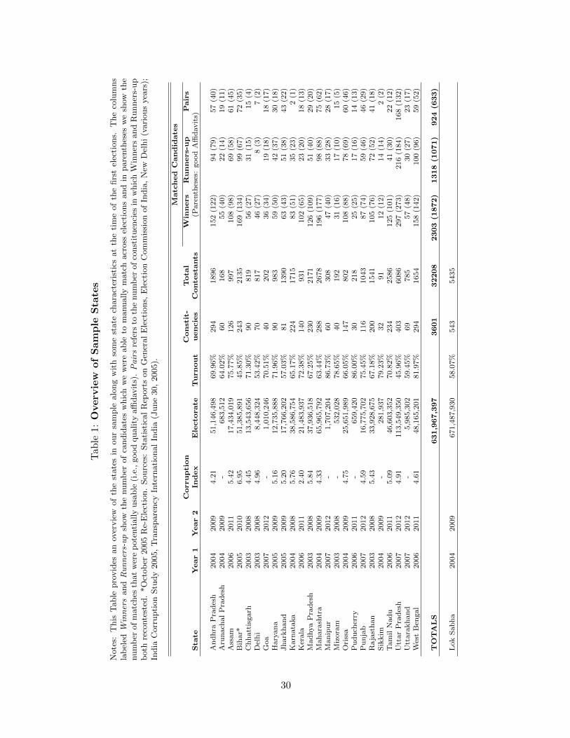
December 2011, covering about 94 percent of India’s total electorate. Table 1 lists the 24

states in our sample along with descriptive information corresponding to the first of the two

elections.

The primary sources for candidate affidavits are the GENESYS Archives of the Election

Commission of India (ECI)4 and the various websites of the Office of the Chief Electoral

Officer in each state. The archives provide scanned candidate affidavits (in the form of

pictures or pdfs) for all candidates, though links to a few affidavits are non-functional. A

sample affidavit is shown in Online Appendix A. Except for the nine elections prior to October

2004, we are able to collect these data from the websites of the National Election Watch which,

in collaboration with ADR, provides digitized candidate affidavits.5 We extended the dataset

by collecting data for the remaining nine elections directly from the scanned affidavits.

In a first step, among all the candidates that contest in the first election in each state,

we filter out the winners and runners-up (our control group) using the Statistical Reports of

Assembly Elections provided by the Election Commission of India (ECI).6 We then match

these winners and runners-up with candidates that contest in the subsequent election in that

state. Due to large commonalities among Indian names as well as different spellings of names

across elections, matching was done manually. Overall, we are able to manually match a total

of 3622 re-contesting candidates (2303 winners and 1319 runners-up) based on variables such

as name, gender, age, education, address, and constituency, as well as a family member’s

name (usually the name of the father or spouse).7

4http://eci.gov.in/archive/5http://www.myneta.info/6http://eci.gov.in/eci main1/ElectionStatistics.aspx7A probabilistic matching algorithm, based on variables such as name and age, proved to be inefficient.To provide an example, in the Tamil Nadu Election of 2006, there are 2 runners-up with identical names

8

Of these initial 3622 matched candidates, we were unable to locate affidavits for both

elections for 53 candidates because of broken weblinks and hence discard them from our

sample. Further, we filter out candidates with affidavits that are poorly scanned, have

missing pages, or handwriting that is too unclear or ambiguous to get a clear picture of a

candidate’s reported financial situation. This drops a total of 561 candidates, or about 15.7

percent of the remaining sample matches.8 Next, we verify suspicious values and, since our

main focus is on growth in wealth, remove candidates that list significant assets without

corresponding market value information, leaving a sample of 2944 matched candidates (1872

winners and 1072 runners-up). Of these 2944 candidates, we have 633 constituencies in which

both the winner and the runner-up re-contest in the following election. This is shown by

state in the last 3 columns of Table 1.

From the affidavits, we compute the candidate’s net wealth, defined as the sum of movable

assets (such as cash, deposits in bank account, and bonds or shares in companies) and

immovable assets (such as agricultural land and buildings) less liabilities (such as loans from

banks), aggregated over all dependent family members listed on the affidavit. Finally, we

remove candidates with negative or extremely low net asset bases using a cutoff of beginning

net worth of Rs 100,000, and Winsorize net asset growth at the first and 99th percentiles.9

This leaves us with a final sample of 2741 matched candidates (1754 winners and 987 runners-

up) of which 1100 are constituency-matched pairs, i.e., we have 550 constituencies in which

both the winner and runner-up recontest.

We define a Criminal Record dummy equal to one if the candidate has pending or past

criminal cases at the time of the first election, and measure education based on years of

schooling (Years of Education). In addition to information gathered from candidates’ affi-

(RAJENDRAN.S), Age (56), and education (10th Pass) despite being identifiably distinct candidates. Wealso commonly encountered differential spellings of names between elections, for instance, Shakeel AhmadKhan (Bihar, 2005) and Shakil Ahmad Khan (Bihar, 2010).

8Affidavit availability and quality differs somewhat across states and tends to be slightly worse in the earlieryears. For example, out of 54 matched candidate in Delhi (2003), 27 percent of affidavits are unavailable orof very poor quality.

9None of these adjustments materially changes the quantitative nature of our results. Our findings are veryrobust to using different cutoff values (e.g., Rs 500,000), trimming instead of Winsorizing, or no adjustmentat all.

9

davits, we also collect data on election victory margins and incumbency from ECI’s Statis-

tical Reports of Assembly Elections. The reports also allow us to classify constituencies as

Scheduled Caste (SC), Scheduled Tribe (ST), or “general” constituencies. SC and ST con-

stituencies are reserved for candidates classified as SC or ST in order to promote members of

historically under-represented groups. That is, general candidates cannot compete in these

SC/ST-designated constituencies. We also distinguish among winning candidates based on

whether they held significant positions in the state government, using an indicator variable

for membership in the Council of Ministers, the state legislature’s cabinet.

As a measure of state-level opportunities for political rent extraction, we obtain a measure

of state-level corruption using the index reported in the 2005 Corruption Study by Trans-

parency International India. This report constructs a corruption index for 20 Indian states

based on perceived corruption in public services using comprehensive survey results for over

10,000 respondents. The index takes on a low value of 240 for the state of Kerala and a high of

695 for Bihar. Our sample covers 17 of the 20 states for which an index value is available and

we rescale the original measure by dividing it by 100. Finally, we collected a cross-section of

state legislature salaries during 2003-2008, and use the Base Salary of politicians to examine

more formally whether official salaries are an important determinant of wealth accumulation.

As we note in the introduction, these official salaries are likely too low to account for the

high levels of wealth accumulation of some politicians.

Table 2 lists definitions of the main variables used in the analysis and in Table 3, we show

some descriptive statistics for our constituency-matched sample of 1100 candidates (Panel

A) as well as for a subsample of elections decided by close margins (Panel B). Average

net assets are about Rs 9.7 million ($194,000 at an exchange rate of Rs 50 per dollar)

for winners and Rs 10.1 million (about $202,000) for runners-up. As a point of reference,

state legislators’ salaries, including allowances, are generally well under Rs 1,000,000 (about

$20,000) with relatively little variation as a function of seniority. Overall, winners and

runners-up in our sample appear to be similar in age, education, and gender. The two

groups differ based on incumbency - incumbents are less likely to win in this sample of

10

re-contestants, consistent with Linden’s (2004) finding of an incumbency disadvantage for

Indian politicians. The only other difference we observe is in net asset growth, which we

will explore in much more detail throughout the paper. About 14 percent of winners are

members of the state Councils of Ministers and 19 percent of the elections in our sample

are from SC/ST-designated constituencies. Runners-up in the subsample of close elections

tend to be slightly more educated than winners on average (14 years of educations vs. 13.8

for winners) though the median years of education is identical. Overall, based on these

observables, runners-up seem to constitute a reasonable comparable control group.10

3 Empirical Framework

Before proceeding to our regression results, it is worth emphasizing what it is that we are

attempting to measure as the returns to public office, and how our sample and specification

plausibly serve to estimate this. We wish to measure the percentage annual growth rate of

assets for an individual elected to public office, relative to the counterfactual where he was

not elected:

Ret. to Public Office = E(Netassetgrowthi|Winneri = 1)−E(Netassetgrowthi|Winneri = 0)

Of course, we cannot measure winner versus loser growth rates for a given politician, but

will rather make a comparison across observed winners and losers. We require that, condi-

tional on observables, assignment to the winner category is independent of returns to winning,

that is, [E(Netassetgrowthi|Winneri = 0),E(Netassetgrowthi|Winneri = 1)]⊥Winneri|Xi.

For the sample of politicians as a whole, this condition clearly fails - for example, politicians

that benefit most from winning will exert the greatest effort in campaigning, and those with

different unobserved (i.e., not in Xi) attributes may be of greater skill.

10On further investigating election expense for a subset of candidates, we also find no material differencesbetween winners and runners-up. Election expenditure on each candidate is further limited by law to aboutRs 1,000,000 in large states, and candidates generally receive lump sum grants from their political parties.

11

The subset of politicians that we may include in our analysis requires the further condition

that they choose to run at the end of an election cycle, regardless of whether they won the

first time around - otherwise, we observe only their initial asset levels, not their growth rates.

Hence, what we can plausibly estimate is the following:

(Ret. to Public Office|Rerun = 1) = E(Netassetgrowthi|Winneri = 1, Rerun = 1)

−E(Netassetgrowthi|Winneri = 0, Rerun = 1)

The independence of winning and the financial returns while in office is at least more

plausible with this subset of the pool of candidates - if these returns were much lower for

Winner = 0 candidates, they may choose not to run again. While this is a relevant subset

of the pool of candidates - those that make a career of running for office - it is likely one for

which the returns to public office are relatively high: if their outside options were sufficiently

good, such candidates may choose not to run again conditional on losing. We discuss this in

more detail in Section 4.4.

This does not necessarily mitigate concerns of unobserved skills correlated with winning,

and also with earnings ability. To make the closest comparison of like candidates, we focus on

a within-constituency comparison of winners and runners-up who choose to run in subsequent

elections, e = 1 and e = 2. This plausibly holds constant labor market opportunities, and

other local attributes affecting the earnings possibilities of winners and runners-up. That is,

we estimate the following fixed effects regression:

Net Asset Growthwc = αc + β ∗Winnerwc + log(NetAssetswc) + Controlswc + εwc (1)

where w ∈ {0, 1} indexes winners and runners-up, c indexes constituencies, αc is a con-

stituency fixed-effect, and εwc is a normally distributed error term.11 In our main empirical

11Note that an alternative formulation would be to ‘first difference’ the data, using the difference betweenwinner and runner-up net asset growth for each constituency as the outcome variable, as a function offirst-differenced covariates. For our main specifications, this approach yields virtually identical results tothose presented here.

12

analysis, we present results on the full within-constituency sample, and also for the subset of

winner/runner-up pairs where the election was decided by a relatively slim margin. We argue

that the within-constituency close election estimation plausibly obviates many concerns of

within-pair unobserved differences.

We also employ a regression discontinuity research design (RDD) as an alternative empiri-

cal strategy, which effectively estimates the winner’s premium based on the winner-runner-up

difference in close elections. Under the identification assumption that outcomes of close elec-

tions are random, the difference in asset growth rates of winners and losers can be causally

attributed to holding public office.

The scatterplots and lines of best fit we show in our figures are produced using common

methods developed in the regression discontinuity literature (e.g., DiNardo and Lee (2004),

Imbens and Lemieux (2008) and Angrist and Pischke (2009)). Specifically, we are interested

in the extent to which winning causes a discontinuity in asset growth residuals at the win-

ning threshold. First we generate residuals by regressing growth in net assets on candidate

observables, including net assets, gender, and age, but excluding winner dummy and margin.

We next collapse the residuals on margin intervals of size 0.5 (margins ranging from -25 to

+25) and then estimate the following specification:

R̄i = α+ τ ·Di + β · f(Margin(i)) + η ·Di · f(Margin(i)) + εi (2)

where R̄i is the average residual value within each margin bin i, Margin(i)) is the mid-

point of margin bin i, Di is an indicator that takes a value of one if the midpoint of margin

bin i is positive and a value of zero if it is negative, and εi is the error term.12 f(Margin(i))

and Di · f(Margin(i)) are flexible fourth-order polynomials. The goal of these functions is

to fit smoothed curves on either side of the suspected discontinuity. The magnitude of the

discontinuity τ is estimated by the difference in the values of the two smoothed functions

12To address heterogeneity in the number of candidates and residual variance within each bin, we weighobservations by the number of candidates, and alternatively by the inverse of within-bin variance. Resultsare similar in both specifications.

13

evaluated at zero.

4 Results

4.1 Graphical presentation of results

We first present a series of figures that provide a visual description of our results. In Figure 1

we plot the Epanechnikov kernel densities of the residuals obtained from regressing growth in

net assets on candidate observables. Panel A uses the entire sample of constituency-matched

candidates while Panel B only uses candidates that were within a margin of 5 percentage

points.13 In both cases, the Kolmogorov-Smirnov test for equality of the distribution function

of winner and runner-up residuals is rejected at the 1 percent level and 5 percent level,

repectively. These figures thus depict a differential effect of election outcomes on net asset

growth between the treatment and control groups. In Panel C, we disaggregate winners

into ministers and non-ministers and plot kernel densities of these two groups as well as the

runners-up. The kernel density plots further suggest a long right tail for ministers, implying

that a relatively small number of these high-level politicians generate very high asset growth.

In Panels D and E, we disaggregate the sample based on whether an incumbent is standing for

reelection in the constituency. Panel D shows winner and runner-up densities for the sample

of constituencies where an incumbent was standing for reelection - the winner distribution is

clearly shifted to the right, implying a greater winner’s premium in races involving incumbents

(a test for equality of the distribution function is rejected at the 1 percent level). Panel E

shows densities for the subsample of non-incumbent constituencies - the winner distribution

is now shifted to the left and a test for equality of the distribution function is rejected at the

10 percent level (p-value of 0.086). We investigate in greater detail the patterns of net asset

growth among incumbents versus non-incumbents in our regression analyses below.

13The chosen bandwidth is the width that would minimize the mean integrated squared error if the data wereGaussian and a Gaussian kernel were used.

14

4.2 Regression Analyses

We now turn to analyze the patterns illustrated in Figure 1 based on the regression framework

described in the prior section. We use the basic specification shown in Equation 1, which

provides a within-constituency estimate of the winner’s premium, and present these results

in Table 4. In the first column, we show the binary within-constituency correlation between

Winner and Net Asset Growth. The coefficient of 0.0296, significant at the 5 percent level,

implies a winner’s premium in asset growth of about 3 percent. Adding log(Net Assets) as

a control in column (2) slightly lowers the point estimate to 0.0291, still significant at the 5

percent level. Column (3) adds controls for gender, incumbency, having a criminal record,

as well as quadratic controls for age and years of education; the point estimate is 0.0265,

significant at the 5 percent level. In columns (4) - (6) we examine the winner’ s premium in

close elections, defined by those where the vote share gap between winner and runner-up was

less than 10, 5, and 3 percentage points. In each case, the winner’s premium is estimated to

be around 3 - 5 percent and significant at the 5 percent level. The point estimate increases

for the 3 percent margin sample, where the coefficient on Winner is 0.0519 and significant

at the 5 percent level (p-value of 0.012).

In Table 5, we consider the returns to office as a function of potential influence in gov-

ernment. In the first column, we add an indicator variable, Minister, denoting whether the

constituency winner was appointed to the state’s Council of Ministers. The point estimate

on Minister is about 0.134, implying a 13.4 percent higher growth rate for Ministers relative

to the runner-up candidates in their constituencies. Further, the coefficient on Winner drops

to very close to zero. The point estimate is 0.01, with a standard error of 0.013, allowing us

to reject a winner’s premium of greater than 4 percent for those not appointed minister, at

the 5 percent level of significance. The results are robust to looking at narrow victory mar-

gins, as indicated by the results in columns (2) - (4). In columns (5) and (6) we include the

interaction of Winner and an indicator variable for whether a candidate’s party was part of

the state government; the small and insignificant coefficient on this interaction term suggests

15

no premium for merely being part of a ruling coalition.14 The coefficient on Minister remains

large and significant, implying extraordinary growth in wealth only for high-level positions.

It is worth emphasizing that it is problematic to assign a causal interpretation to the corre-

lation between Minister status and returns, since assignment to these posts is non-random.

At the same time, the very large effect of holding a Minister position on asset returns is such

that it is not easily explained by unobserved differences in abilities, and warrants further

investigation in future work.

In columns (7) and (8) we disaggregate asset growth into Movable Asset Growth through

holdings such as cash, bank deposits, and jewelry, and Immovable Asset Growth from land

and building assets (see the full definition in the Data section). We see a sharp difference

between the asset growth of Minister versus non-Minister politicians. The coefficient on

Winner is a highly significant predictor of growth in movable assets, implying a winner’s

premium of 5.23 percent. The magnitude of the coefficient on Minister in (7) implies a

further premium in movable asset growth of 4.2 percent, though this effect is not significant.

For immovable assets, the Minister growth premium is 8.8 percent and significant at the 10

percent level, while the winner’s premium is small in magnitude and statistically insignificant.

Note that immovable assets constitute, on average, about three quarters of a candidate’s

total assets. If the asset growth of politicians is the result of extra-legal payments, this

difference may simply reflect the fact that the scale of gifts is larger for ministers (e.g., cars

versus buildings). It may also result from access to low cost purchase of land for high-level

individuals as suggested by, for example, the case of Karnataka’s former Chief Minister B.S.

Yeddyurappa, who acquired land parcels at extremely favorable prices before selling them off

to mining companies.15 Such opportunities may only be available to high-ranking politicians.

In Table 6 we turn to assess how the winner’s premium differs as a function of incumbency,

by including the interaction term Winner*Incumbent. As suggested by the patterns in Fig-

14We also considered the effect of membership in the two main political parties - the Congress and the BJP -on the winner’s premium. The Winner*Congress interaction was marginally significant and positive, whilethe interaction of Winner*BJP was negative, though not significant at conventional levels.

15“Ministers stole millions in Karnataka mining scam,” BBC South Asia, July 21, 2011

16

ure 1, the winner’s premium comes exclusively from incumbents. The coefficient on Winner

is -0.053 and significant at the 5 percent level, implying that non-incumbent winners’ asset

growth is 5.3 percent lower than that of non-incumbent runners-up. The pattern is reversed

for incumbents, where there is a winner’s premium of nearly 12.6 percent (the sum of the

coefficients on Winner and Winner*Incumbent). One plausible interpretation of this differ-

ential winner’s premium by incumbency is that it reflects the relatively limited private sector

options available to career politicians. Alternatively, it may result from the greater skill with

which incumbents extract value from political office. The data are at least suggestive of the

first of these explanations - the large winner’s premium for incumbents is primarily the result

of the low earnings of incumbents that are not returned to office: incumbent winners have a

median asset growth of 0.205, virtually identical the median asset growth of non-incumbents

overall (0.204), while the median asset growth of incumbent runners-up is 0.15.

4.2.1 Electoral Accountability

The extent that legislators extract financial returns from their positions may be limited by

pressure from the electorate, particularly given the transparency afforded by the Right to

Information Act. We emphasize that the asset growth calculations we perform here are based

on data easily accessible via the internet, and their availability has been widely reported in

the Indian media. In Table 7 we examine whether there is any effect of high asset growth on

election outcomes, through the following specification:

Reelectionwc = αc + β1 ∗Winnerwc + β2 ∗Net Asset Growthwc (3)

+β3 ∗Winnerwc ∗Net Asset Growthwc + εwc

where Reelectionwc is an indicator variable that takes on a value of 1 if the candidate

won election e = 2 and 0 otherwise. While none of the coefficients are significant, the results

point, if anything, in the opposite direction - the coefficient on Net Asset Growth is positive

in Column (1), and its interaction with Winner, capturing the effect of asset growth among

17

election winners, is positive (Column 2). In results not reported, we also find that legislators

who win by large margins do not earn a higher winner’s premium. Such a specification

is, however, subject to extreme problems of unobserved heterogeneity - the large margin

may be because of a candidate’s effort or political skill, confusing the interpretation of the

Winner*Margin interaction. Finally, the negative coefficient on Winner is consistent with a

negative incumbency effect in India that was already observed in Table 3.

4.2.2 Exploring Cross-sectional Heterogeneity

In Table 8 we examine heterogeneity in the winner’s premium as a function of a number of

other candidate characteristics. In column (1) we look at the effect of state-level Corrup-

tion. The coefficient on the interaction term Winner*Corruption, while positive and hence

implying a higher winner’s premium in more corrupt states, is not statistically significant.

In column (2) we allow for a Minister*Corruption interaction; the coefficient on this term is

positive, again implying a larger asset growth premium in more corrupt states, but also not

significant. In column (3) we consider whether candidates with prior criminal records have

a higher winner’s premium. The coefficient on the interaction term is not significant.

In column (4) we consider the set of constituencies reserved for members of disad-

vantaged groups, so-called Scheduled Tribes and Castes (SC/ST). The interaction term

SC/ST Quota∗Winner is significant at the 1 percent level, and implies a winner’s premium

in asset growth of about 8 to 9 percent for constituencies reserved for SC/ST candidates.

There are two primary explanations for the relatively high winner’s premium for SC/ST-

designated constituencies. First, since these seats are reserved for a subset of potential

candidates, it may slacken electoral competition, allowing candidates to extract greater rents

without fear of losing their positions. Alternatively, SC/ST politicians may have less lucrative

private sector options as a result of discrimination, lower unobserved skill levels, or weaker

labor market opportunities in SC/ST-dominated areas. While we cannot include both the

direct effect of SC/ST Quota and constituency fixed effects in a single specification, in

18

column (5) we look at the direct effect of SC/ST quotas with a coarser set of fixed effects, at

the district level. There are approximately half as many districts as constituencies in our main

sample. We find a very similar coefficient on the interaction term SC/ST Quota ∗Winner

in this specification - approximately 0.09 - while the direct effect of SC/ST Quota is -0.073.

That is, it would appear that among runners-up, SC/ST politicians fare significantly worse

than other candidates, providing suggestive evidence that the differential SC/ST effect results

in large part from different private sector opportunities.

In column (7), we examine the effects of candidates’ education levels by including as

covariates the logarithm of years of schooling as well as its interaction with Winner. We

find a small positive direct effect of years of schooling, implying that for runners-up, asset

growth is higher for more educated candidates. However, this is more than offset by the in-

teraction term, log(Years of Education)*Winner. The sum of the coefficients on log(Years of

Education) and its interaction with Winner, while negative, is not significant at conventional

levels. This is broadly consistent with highly educated candidates having better private

sector opportunities, but not greater earning capacity as public officials.

We show the interaction of Female and Winner in column (6). The coefficient is positive,

though not statistically significant. Finally, in column (8) we interact Winner with log(Base

Salary). We find no evidence that the winner’s premium is higher in states with more

generous official salaries for legislators, implying that it is unlikely that official salaries play

a major role in the differential asset accumulation of elected officials.

4.3 Regression Discontinuity Design

Our main empirical identification strategy is effectively based on a regression discontinuity

design, with the winner’s premium identified from the winner-loser differential in close elec-

tions . In this section, we explicitly model the value of winning using regression discontinuity

methods, as described in Section 3. We first show a series of figures that depict our tests

for discontinuities around the winning threshold, followed by an analysis of the magnitudes

19

of winner-loser discontinuities. Note that we follow the approach outlined in Section 4.1 by

looking at net asset growth residuals which allows us to control for remaining differences in

covariates of candidates as well as observed and unobserved constituency heterogeneity. The

methodology in this section can thus be considered as conditional RD. Results are quantita-

tively similar when (unconditional) net asset growth in used.

In Figure 2, Panels A - E, we provide a visual description of this analysis and columns (1)

- (5) of Table 9 provide the corresponding discontinuity estimates of the winner’s premium.16

Panel A shows the sample of all winners and corresponding runners-up. Our estimated

regression indicates a jump in the residual values around the threshold. The point estimate

of τ is 0.065, and statistically significant at the 1 percent level (t-statistic of 2.8). Panel B only

includes ministers with corresponding runners-up - the point estimate of the discontinuity

increases to 0.287 (t-statistic of 5.26), a result qualitatively similar to that of the regression

analysis in the previous section, though somewhat larger in magnitude. On the other hand,

the subsample of winners not appointed to a Council of Ministers and corresponding runners-

up does not indicate a jump at all (Panel C) - the coefficient estimate of the discontinuity

is 0.0265 with a t-statistic of 1.13. In Panels D and E, we disaggregate the sample based on

whether an incumbent is standing for reelection in the constituency. Panel D shows results for

the sample of constituencies where an incumbent was running for reelection. The coefficient

estimate of the discontinuity is 0.08 and significant at the 1 percent level (t-statistic of 3.19).

By contrast, for the sample of non-incumbent constituencies, we observe no jump at the

threshold (the point estimate is 0.028 with a t-statistic of 0.79). Overall, these results are in

line with those obtained from standard regression analysis.

Finally, in Figure 3 we plot kernel densities of age and log(Net Assets) for the sample of

constituency-matched candidates that were within a Margin of 5 percentage points (“close

elections”). Panel A plots age densities for winners and runners-up and Panel B plots densities

for log(Net Assets). For both observables, the Kolmogorov-Smirnov test for equality of the

16Note that the apparent symmetries in the RD plots are the result of constituency fixed effects. Including con-stituency fixed effects allows us to control for observable and unobservable constituency-level heterogeneity,for example, differences in local labor markets or SC/ST Quota.

20

distribution function of winners and runners-up cannot be rejected at conventional levels,

providing some validation of our regression discontinuity design.

Based on these discontinuities, we can perform a simple back-of-the envelope calculation

to to approximate the winner’s premium in monetary terms. We do this by first calculating

how winners’ average wealth would have grown had they not won the election using the net

asset growth rate of all constituency-matched runners-up, and then comparing this average

to the level of wealth accumulation using the discontinuity estimates from the RD design.

Overall, for Winners as a group, the estimated annual premium is approximately Rs 1,500,000

(USD 30,000). However, for Ministers the winner premium is significantly larger, about Rs

10,750,000 per year (USD 215,000). By comparison, state-level legislators have salaries that

are much lower - generally under Rs 1,000,000 per year (USD 20,000). Further, these wealth

accumulation increments are relative to candidates’ initial assets that are, on average, only

about Rs 10,000,000 (USD 200,000), implying a very large impact in percentage terms.

4.4 Addressing Selection

Our analysis compares the returns of winners versus runners-up in constituencies where

both candidates run in two consecutive elections. While this sample allows us to include

constituency fixed effects and thus control for local constituency-level omitted variables, it

is important to consider whether these results are external valid for Indian legislators more

generally.

At the outset, we note that the constituencies that constitute our sample - where both

the winner and the runner-up contest both elections - are very similar on observables to

constituencies where only one of the candidates recontests. Specifically, the mean electorate,

percentage turnout, and percent SC/ST population for our winner/runner-up matched con-

stituencies are not significantly different from the rest of the population. Candidates in these

constituencies are also quite similar in attributes such as log of assets, age, and education.17

17For brevity, tables are not shown but are available from the authors upon request.

21

Thus, we believe that the local average treatment effects documented above can be likely

generalized to the population.

As noted earlier, our identification strategy – comparing candidates from the same con-

stituency in close elections – attempts to control for unobserved ability differences in can-

didates. By comparing the net asset growth of two otherwise similar candidates following

an election where one prevails by a narrow margin, we may calculate the private returns to

public office relative to a similar candidate that just lost the election. One significant concern

with this approach, however, is that electoral victory may itself influence the probability of

recontesting, and hence inclusion in the sample. Indeed, in Panel A of Figure 4, we find

that runners-up have a lower probability of re-contesting the second election when compared

to the corresponding constituency winners. The probability of recontesting is increasing in

margin, with a clear discontinuity at zero.18

In considering how this differential exit rate may affect our results, we note first that it

is not obvious a priori which direction any selection effect would bias our estimates. One

one hand, winners and runners-up that re-contest the second election are plausibly more

similar in terms of political ability than pairs where both contest the first election but one

subsequently chooses not to contest the second election. In this case, one might expect

that the ability differences between winners and runners-up are smaller in our sample of

constituencies than those without matched winners/runners-up, hence biasing our results

towards zero. 19 Alternatively, if candidates that exit have higher outside options compared

18In a separate analysis (not reported for brevity), we examine the recontesting decision of political candidatesusing a simple probit model. The dependent variable is one if we can match the candidate in a subsequentelection and zero if we only observe a candidate at election 1. We conduct our analysis separately for thesub-samples of winners and runners-up, and find that candidates that win the first election are significantlymore likely to re-contest in the subsequent election. For the sub-samples of both winners and runners-up,we find that wealthier and more educated candidates are more likely to rerun, whereas age is negativelyrelated to the decision to re-contest. The only variable that affects both groups differently is the winningmargin at the first election – runners-up who lose by wider margins are significantly less likely to re-contest,whereas for winners margin is not a significant predictor of running in the next election. There are twoready explanations for this difference - (1) if a candidate loses by a large margin, he may re-evaluate hischances of winning and not re-contest a second time, or (2) he may not get chosen to represent his party ifhe has shown little success in the previous attempt.

19Runners-up and winners in our sample have virtually identical chances of succeeding in the subsequentelection (42.08 percent and 41.89 percent, respectively), providing further support for similar political abilityof the two groups.

22

to candidates that decide to re-contest, neglecting the asset growth of unsuccessful candidates

that do not rerun may bias our analysis towards finding an effect even when none exists.

4.4.1 Evidence from Seasoned Candidates

To further assess the influence that differential exit rates may have on the estimated winner’s

premium, we analyze a restricted sample of constituencies where both winner and runner-

up are seasoned politicians, in the sense of both competing in at least two elections prior

to the elections we consider in our analysis, and where both were either winner or runner-

up in these earlier elections. Repeated contests of this sort between seasoned politicians

is surprisingly common in our sample. We provide one illustrative example below for the

Biswanath Assembly Constituency in the state of Assam. In this case, both candidates,

Prabin Hazarika and Nurjamal Sarkar, have contested all elections since 1991 and have been

either a winner or a runner-up in each instance. We argue that such career politicians are

less likely to exit because of party decisions or a reevaluation of future electoral success -

by construction, we include only politicians who have performed well as candidates in the

recent past. This subset of active seasoned politicians arguably represent more comparable

treatment and control candidates than the full sample of re-contesting politicians.

Biswanath Assembly Constituency (Assam)Year Winner %age Party Runner-up %age Party

2011 Prabin Hazarika 45.51 AGP Nurjamal Sarkar 44.09 INC2006 Nurjamal Sarkar 41.76 INC Prabin Hazarika 39.46 AGP2001 Nurjamal Sarkar 48.55 INC Prabin Hazarika 44.3 AGP1996 Prabin Hazarika 42.62 AGP Nurjamal Sarkar 31.76 INC1991 Nurjamal Sarkar 46.49 INC Prabin Hazarika 17.39 AGP

We focus our analysis on this set of active seasoned candidates in Panels B and C of

Figure 4. In Panel B, we find no differential probability of re-contesting the second election;

however, Panel C documents a jump in net asset growth rates around the winning threshold.

The point estimate of the discontinuity is 0.12 and significant at the 5 percent level. This is

consistent with differential exit rates of winners and runners-up creating a downward bias in

23

our main estimates on the returns to public office.

4.4.2 Evidence from Bihar’s Hung Parliament

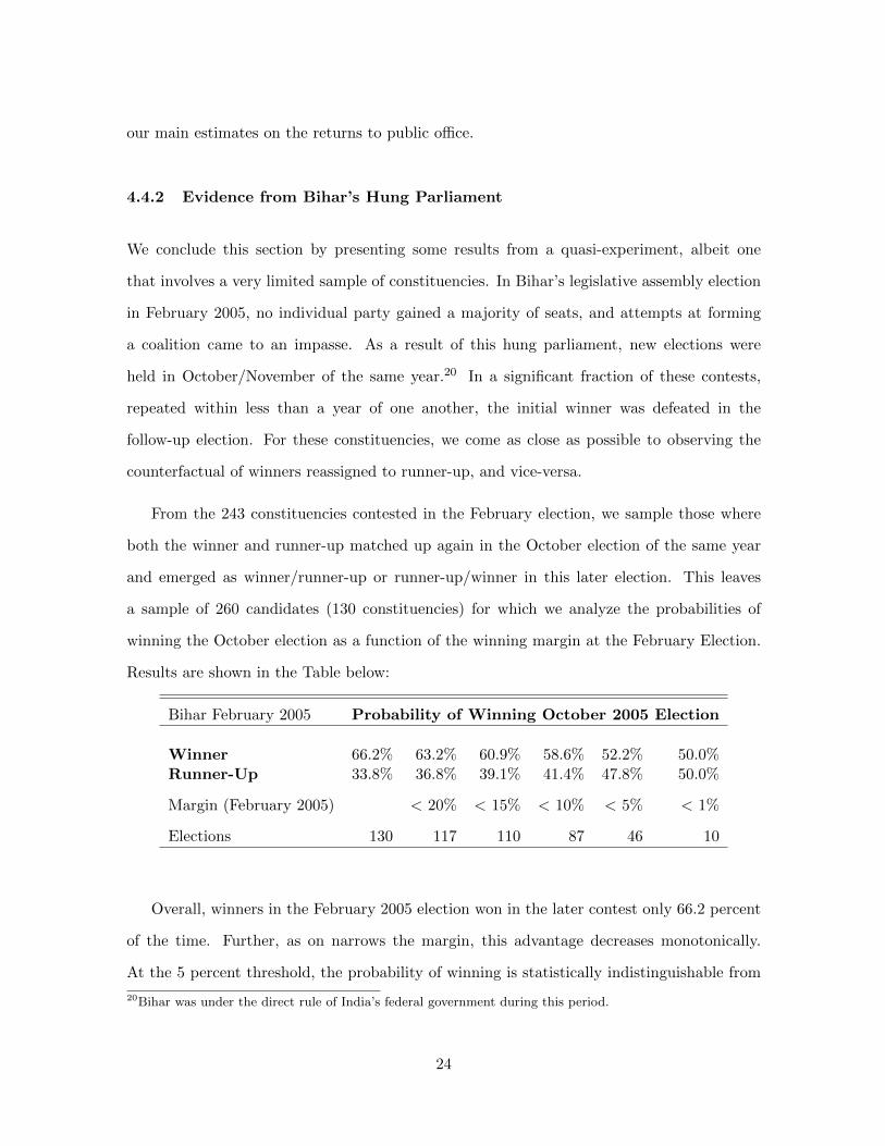
We conclude this section by presenting some results from a quasi-experiment, albeit one

that involves a very limited sample of constituencies. In Bihar’s legislative assembly election

in February 2005, no individual party gained a majority of seats, and attempts at forming

a coalition came to an impasse. As a result of this hung parliament, new elections were

held in October/November of the same year.20 In a significant fraction of these contests,

repeated within less than a year of one another, the initial winner was defeated in the

follow-up election. For these constituencies, we come as close as possible to observing the

counterfactual of winners reassigned to runner-up, and vice-versa.

From the 243 constituencies contested in the February election, we sample those where

both the winner and runner-up matched up again in the October election of the same year

and emerged as winner/runner-up or runner-up/winner in this later election. This leaves

a sample of 260 candidates (130 constituencies) for which we analyze the probabilities of

winning the October election as a function of the winning margin at the February Election.

Results are shown in the Table below:

Bihar February 2005 Probability of Winning October 2005 Election

Winner 66.2% 63.2% 60.9% 58.6% 52.2% 50.0%Runner-Up 33.8% 36.8% 39.1% 41.4% 47.8% 50.0%

Margin (February 2005) < 20% < 15% < 10% < 5% < 1%

Elections 130 117 110 87 46 10

Overall, winners in the February 2005 election won in the later contest only 66.2 percent

of the time. Further, as on narrows the margin, this advantage decreases monotonically.

At the 5 percent threshold, the probability of winning is statistically indistinguishable from

20Bihar was under the direct rule of India’s federal government during this period.

24

50 percent for either candidate. This suggests a significant element of randomness to close

elections in this sample.21

To further sharpen our empirical strategy, we compare the net asset growth of two groups

– the treatment and control groups. The treatment group consists of candidates that were

runners-up in the February 2005 election but won in the October 2005 contest, while the

control group is comprised of candidates that were winners in February 2005 but runners-

up in the October election. These cases where winners and losers were switched owing to

the hung parliament provides a measure of the returns to public office with a relatively

straightforward causal interpretation. We look at all such candidates whose winner status

shifted between these two 2005 elections, and also chose to run again in 2010, so we can

calculate their asset growth rates. The resulting set of candidates is relatively small - 25

winners and 26 runners-up - which limits the types of statistical tests one can perform on

this sample. For this subset of candidates we find that the annual net asset growth of the

treatment group is on average 12.76% higher than that of the control group, a difference that

is significant at the 5 percent level. If we limit ourselves only to the constituency matched

samples where winner and runner-up status switched and both candidates ran in the 2010

election, the sample is reduced to 11 constituencies - 22 candidates - and we find a difference

in the net asset growth between winners and runners-up of approximately 6 percent, roughly

similar to the magnitudes we observe with the full sample. Given the small sample size, the

difference in asset growth for the sample of 22 candidates is not statistically significant.

5 Conclusion

In this paper, we utilize the asset disclosures of candidates for Indian state legislatures,

taken five years apart at two points across a five year election cycle, and accessed through

21Recent papers by Snyder (2005), Caughey and Sekhon (2010), Carpenter et al. (2011), and Folke et al.(2011) critically assess regression discontinuity studies that rely on close elections. There remains an activedebate on whether close elections can really be considered a matter of random assignment. If sorting aroundthe winning threshold is not random, but close winners have systematic advantages, then the RD designmay fail to provide valid estimates of the returns to office. The Bihar example provides at least suggestiveevidence that close elections are relatively random in the context we consider in this paper.

25

the country’s Right to Information Act. This has allowed us to compare the asset growth

of election winners versus runners-up to calculate the financial returns from holding public

office relative to private sector opportunities available to career politicians.

Our main findings suggest, at least in the Indian context, a relatively limited financial

benefit of public office for most politicians. By contrast, we find a 13-29 percent growth

premium for ministers in our sample, suggesting very strong earnings possibilities for higher-

level politicians. Looking at election winners not appointed to the Council of Ministers,

the asset growth premium for election winners is about one percent per year. Further,

this premium is derived entirely from the winner-loser differential among incumbents, with

incumbent runners-up earning unusually low returns when confronted with private sector job

opportunities; for non-incumbents, the winner’s premium is negative.

These findings have a number of implications for the modeling of the political process and

politicians’ behavior. First, our results suggest a sharp difference in the value of influencing

legislators at different levels in the Indian hierarchy: the votes of individual legislators have

relatively low value for private agents, while the influence of ministers is potentially very

valuable. At least in financial terms, one may thus think about prospective politicians being

motivated more by future rewards from gaining higher positions than by the initial returns of

holding office. This is broadly consistent with a tournament model of politics in the spirit of

Lazear and Rosen (1981), where participants compete for the high returns that only a small

fraction of entry-level politicians will attain.

Our work also presents several possible directions for future work. Given the high returns

we observe among ministers, it may be fruitful, with the benefit of additional data, to examine

whether particular positions within the Council are associated with high rents. And while

we do not observe a strong sensitivity of election outcomes to asset growth, one may assess

whether electoral accountability is affected by voter exposure to asset data, in the spirit of

Banerjee et al (2011). It may be interesting to explore the impact of the Right to Information

Act itself: disclosure requirements may induce exit by winners that have extracted high rents,

26

in order to avoid possible corruption-related inquiries. Finally, we are unable in this work to

uncover the mechanism through which asset accumulation takes place. We leave these and

other extensions for future work, which will be enabled either by experimental intervention

or the accumulation of new data via the Right to Information Act.

27

References

[1] Angrist, Joshua and Jorn-Steffen Pischke, 2009, Mostly Harmless Econometrics, Princeton Uni-

versity Press, Princeton, NJ.

[2] Banerjee, Abhijit V., Selvan Kumar, Rohini Pande and Felix Su, 2011, Do Informed Voters Make

Better Choices? Experimental Evidence from Urban India, Working Paper.

[3] Barro, Robert, 1973, The Control of Politicians: An Economic Model, Public Choice 14:19-42.

[4] Besley, Timothy, 2004, Paying Politicians: Theory and Evidence, Journal of the European Eco-

nomic Association, 2, 193-215.

[5] Bhavnani, Rikhil R., 2012, Using Asset Disclosures to Study Politicians Rents: An Application

to India, Working Paper.

[6] Braguinsky, Serguey , Sergey Mityakov, and Andrey Liscovich, 2010, Direct Estimation of Hidden

Earnings: Evidence From Administrative Data, Working Paper.

[7] Buchanan, James, 1989, The Public Choice Perspective, in Essays on the Political Economy,

Honolulu: University of Hawaii Press.

[8] Carpenter, David, Brian Feinstein, Justin Grimmer and Eitan Hersh, 2011, Are Close Elections

Random?, Working Paper.

[9] Caselli, Francesco and Massimo Morelli, 2004, Bad Politicians, Journal of Public Economics 88,

759-782.

[10] Caughey, Devin M. and Jasjeet S. Sekhon, 2010, Regression-Discontinuity Designs and Popular

Elections: Implications of Pro-Incumbent Bias in Close U.S. House Races, Working Paper.

[11] Diermeier, Daniel, Michael Keane and Antonio Merlo, 2005, A Political Economy Model of Con-

gressional Careers, American Economic Review 95(1): 347373.

[12] DiNardo, John and David S. Lee, 2004, Economic Impacts of New Unionization on Private Sector

Employees: 1984-2001, Quarterly Journal of Economics 119, 1383-1441.

[13] Eggers, Andrew and Jens Hainmueller, 2009, MPs for Sale? Estimating Returns to Office in

Post-War British Politics, American Political Science Review, 103(4): 513-533.

[14] Eggers, Andrew and Jens Hainmueller, 2010, Political Investing: The Common Stock Investments

of Members of Congress 2004-2008, Working Paper.

28

[15] Ferejohn, John, 1986, Incumbent Performance and Electoral Control, Public Choice 50: 5-25.

[16] Ferraz, Claudio and Frederico Finan, 2011, Electoral Accountability and Corruption: Evidence

from the Audits of Local Governments, American Economic Review 101, 12741311.

[17] Fisman, Raymond J., Nikolaj Harmon, Emir Kamenica and Inger Munk, 2011, Labor Supply of

Politicians, Working Paper.

[18] Folke, Olle, Shigeo Hirano and James M. Snyder, Jr, 2011, A Simple Explanation for Bias at the

50-50 Threshold in RDD Studies Based on Close Elections, Working Paper.

[19] Gagliarducci, Stefano and Tommaso Nannicini, forthcoming, Do Better Paid Politicians Perform

Better? Disentangling Incentives from Selection, Journal of the European Economic Association.

[20] Imbens, Guido and Thomas Lemieux, 2008, Regression Discontinuity Designs: A Guide to Prac-

tice, Journal of Econometrics 142(2) 615-635.

[21] Kotakorpi, Kaisa and Panu Poutvaara, 2011, Pay for Politicians and Candidate Selection: An

Empirical Analysis, Journal of Public Economics 95 (7-8): 877-885.

[22] Lazear, Edward P. and Sherwin Rosen, 1981, Rank-Order Tournaments as Optimum Labor Con-

tracts, Journal of Political Economy 89(5): 841-864.

[23] Linden, Leigh, 2004, Are Incumbents Always Advantaged? The Preference for Non-Incumbents

in India, Working Paper.

[24] Lenz, Gabriel, and Kevin Lim, 2009, Getting Rich(er) in Office? Corruption and Wealth Accu-

mulation in Congress, Working Paper.

[25] Matozzi, Andrea and Antonio Merlo, 2008, Political Careers or Career Politicians?, Journal of

Public Economics 92(3-4), pages 597-608.

[26] Olken, Benjamin and Rohini Pande, 2012, Corruption in Developing Countries, Working Paper.

[27] Querubin, Pablo and James Snyder, Returns to U.S. Congressional Seats in the Mid-19th Cen-

tury, in The Political Economy of Democracy, Enriqueta Aragones, Carmen Bevia, Humberto

Llavador, and Norman Schofield (eds.), 2009.

[28] Snyder, Jason, 2005, Detecting Manipulation in U.S. House Elections, Working Paper.

[29] Ziobrowski, Alan J., James W. Boyd, Ping Cheng and Brigitte J.Ziobrowski, 2011, Abnormal

Returns From the Common Stock Investments of Members of the U.S. House of Representatives,

Business and Politics: Vol. 13: Iss. 1, Article 4.

29

Tab

le1:

Overv

iew

of

Sam

ple

Sta

tes

Note

s:T

his

Table

pro

vid

esan

over

vie

wof

the

state

sin

our

sam

ple

alo

ng

wit

hso

me

state

chara

cter

isti

csat

the

tim

eof

the

firs

tel

ecti

ons.

The

colu

mns

lab

eled

Winners

andRunners-up

show

the

num

ber

of

candid

ate

sw

hic

hw

ew

ere

able

tom

anually

matc

hacr

oss

elec

tions

and

inpare

nth

eses

we

show

the

num

ber

of

matc

hes

that

wer

ep

ote

nti

ally

usa

ble

(i.e

.,good

quality

affi

dav

its)

.Pairs

refe

rsto

the

num

ber

of

const

ituen

cies

inw

hic

hW

inner

sand

Runner

s-up

both

reco

nte

sted

.*O

ctob

er2005

Re-

Ele

ctio

n.

Sourc

es:

Sta

tist

ical

Rep

ort

son

Gen

eral

Ele

ctio

ns,

Ele

ctio

nC

om

mis

sion

of

India

,N

ewD

elhi

(vari

ous

yea

rs);

India

Corr

upti

on

Stu

dy

2005,

Tra

nsp

are

ncy

Inte

rnati

onal

India

(June

30,

2005).

Matc

hed

Can

did

ate

s

Corru

pti

on

Con

stit

-T

ota

lW

inn

ers

Ru

nn

ers-

up

Pair

sS

tate

Year

1Y

ear

2In

dex

Ele

cto

rate

Tu

rn

ou

tu

en

cie

sC

onte

stants

(Pare

nth

eses

:good

Affi

davit

s)

An

dh

raP

rad

esh

2004

2009

4.2

151,1

46,4

98

69.9

6%

294

1896

152

(122)

94

(79)

57

(40)

Aru

nach

al

Pra

des

h2004

2009

-683,5

12

64.0

2%

60

168

55

(40)

22

(14)

19

(11)

Ass

am

2006

2011

5.4

217,4

34,0

19

75.7

7%

126

997

108

(98)

69

(58)

61

(45)

Bih

ar*

2005

2010

6.9

551,3

85,8

91

45.8

5%

243

2135

169

(134)

99

(67)

72

(35)

Ch

hatt

isgarh

2003

2008

4.4

513,5

43,6

56

71.3

0%

90

819

56

(27)

31

(15)

15

(4)

Del

hi

2003

2008

4.9

68,4

48,3

24

53.4

2%

70

817

46

(27)

8(3

)7

(2)

Goa

2007

2012

-1,0

10,2

46

70.5

1%

40

202

36

(34)

19

(18)

18

(17)

Hary

an

a2005

2009

5.1

612,7

35,8

88

71.9

6%

90

983

59

(50)

42

(37)

30

(18)

Jh

ark

han

d2005

2009

5.2

017,7

66,2

02

57.0

3%

81

1390

63

(43)

51

(38)

43

(22)

Karn

ata

ka

2004

2008

5.7

638,5

86,7

54

65.1

7%

224

1715

83

(51)

35

(23)

2(1

)K

erala

2006

2011

2.4

021,4

83,9

37

72.3

8%

140

931

102

(65)

23

(20)

18

(13)

Mad

hya

Pra

des

h2003

2008

5.8

437,9

36,5

18

67.2

5%

230

2171

126

(109)

51

(40)

29

(20)

Mah

ara

shtr

a2004

2009

4.3

365,9

65,7

92

63.4

4%

288

2678

196

(177)

98

(88)

75

(62)

Man

ipu

r2007

2012

-1,7

07,2

04

86.7

3%

60

308

47

(40)

33

(28)

28

(17)

Miz

ora

m2003

2008

-532,0

28

78.6

5%

40

192

31

(16)

17

(10)

15

(5)

Ori

ssa

2004

2009

4.7

525,6

51,9

89

66.0

5%

147

802

108

(88)

78

(69)

60

(46)

Pu

du

cher

ry2006

2011

-659,4

20

86.0

0%

30

218

25

(25)

17

(16)

14

(13)

Pu

nja

b2007

2012

4.5

916,7

75,7

02

75.4

5%

116

1043

87

(74)

59

(46)

46

(29)

Ra

jast

han

2003

2008

5.4

333,9

28,6

75

67.1

8%

200

1541

105

(76)

72

(52)

41

(18)

Sik

kim

2004

2009

-281,9

37

79.2

3%

32

91

12

(12)

14

(14)

2(2

)T

am

ilN

ad

u2006

2011

5.0

946,6

03,3

52

70.8

2%

234

2586

125

(101)

41

(30)

22

(12)

Utt

ar

Pra

des

h2007

2012

4.9

1113,5

49,3

50

45.9

6%

403

6086

297

(273)

216

(184)

168

(132)

Utt

ara

kh

an

d2007

2012

-5,9

85,3

02

59.4

5%

69

785

57

(48)

30

(27)

23

(17)

Wes

tB

engal

2006

2011

4.6

148,1

65,2

01

81.9

7%

294

1654

158

(142)

100

(96)

59

(52)

TO

TA

LS

631,9

67,3

97

3601

32208

2303

(1872)

1318

(1071)

924

(633)

Lok

Sab

ha

2004

2009

671,4

87,9

30

58.0

7%

543

5435

30

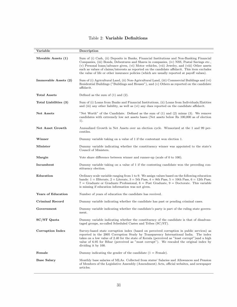
Table 2: Variable Definitions

Variable Description

Movable Assets (1) Sum of (i) Cash, (ii) Deposits in Banks, Financial Institutions and Non-Banking FinancialCompanies, (iii) Bonds, Debentures and Shares in companies, (iv) NSS, Postal Savings etc.,(v) Personal loans/advance given, (vi) Motor vehicles, (vii) Jewelry, and (viii) Other assetssuch as values of claims/interests as reported on the candidate affidavit. This item excludesthe value of life or other insurance policies (which are usually reported at payoff values).

Immovable Assets (2) Sum of (i) Agricultural Land, (ii) Non-Agricultural Land, (iii) Commercial Buildings and (vi)Residential Buildings (”Buildings and Houses”), and (v) Others as reported on the candidateaffidavit.

Total Assets Defined as the sum of (1) and (2).

Total Liabilities (3) Sum of (i) Loans from Banks and Financial Institutions, (ii) Loans from Individuals/Entitiesand (iii) any other liability, as well as (vi) any dues reported on the candidate affidavit.

Net Assets ”Net Worth” of the Candidate. Defined as the sum of (1) and (2) minus (3). We removecandidates with extremely low net assets bases (Net assets below Rs 100,000 as of election1).

Net Asset Growth Annualized Growth in Net Assets over an election cycle. Winsorized at the 1 and 99 per-centiles.

Winner Dummy variable taking on a value of 1 if the contestant won election 1.

Minister Dummy variable indicating whether the constituency winner was appointed to the state’sCouncil of Ministers.

Margin Vote share difference between winner and runner-up (scale of 0 to 100).

Incumbent Dummy variable taking on a value of 1 if the contesting candidate won the preceding con-stituency election.

Education Ordinary scale variable ranging from 1 to 9. We assign values based on the following educationbands: 1 = Illiterate, 2 = Literate, 3 = 5th Pass, 4 = 8th Pass, 5 = 10th Pass, 6 = 12th Pass,7 = Graduate or Graduate Professional, 8 = Post Graduate, 9 = Doctorate. This variableis missing if education information was not given.

Years of Education Number of years of education the candidate has received.

Criminal Record Dummy variable indicating whether the candidate has past or pending criminal cases.

Government Dummy variable indicating whether the candidate’s party is part of the ruling state govern-ment.

SC/ST Quota Dummy variable indicating whether the constituency of the candidate is that of disadvan-taged groups, so-called Scheduled Castes and Tribes (SC/ST).

Corruption Index Survey-based state corruption index (based on perceived corruption in public services) asreported in the 2005 Corruption Study by Transparency International India. The indextakes on a low value of 2.40 for the state of Kerala (perceived as ”least corrupt”)and a highvalue of 6.95 for Bihar (perceived as ”most corrupt”). We rescaled the original index bydividing it by 100.

Female Dummy indicating the gender of the candidate (1 = Female).

Base Salary Monthly base salaries of MLAs. Collected from states’ Salaries and Allowances and Pensionof Members of the Legislative Assembly (Amendment) Acts, official websites, and newspaperarticles.

31

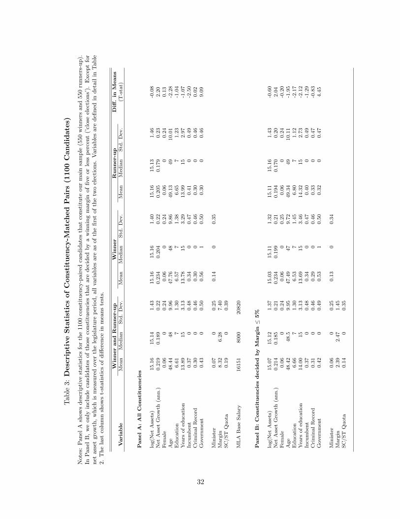
Tab

le3:

Desc

rip

tive

Sta

tist

ics

of

Con

stit

uen

cy-M

atc

hed

Pair

s(1

100

Can

did

ate

s)

Note

s:P

anel

Ash

ows

des

crip

tive

stati

stic

sfo

rth

e1100

const

ituen

cy-p

air

edca

ndid

ate

sth

at

const

itute

our

main

sam

ple

(550

win

ner

sand

550

runner

s-up).

InP

anel

B,

we

only

incl

ude

candid

ate

sof

those

const

ituen

cies

that

are

dec

ided

by

aw

innin

gm

arg

inof

five

or

less

per

cent

(’cl

ose

elec

tions’

).E

xce

pt

for

net

ass

etgro

wth

,w

hic

his

mea

sure

dov

erth

ele

gis

latu

rep

erio

d,

all

vari

able

sare

as

of

the

firs

tof

the

two

elec

tions.

Vari

able

sare

defi

ned

indet

ail

inT

able

2.

The

last

colu

mn

show

st-

stati

stic

sof

diff

eren

cein

mea

ns

test

s.

Win

ner

an

dR

un

ner-u

pW

inn

er

Ru

nn

er-u

pD

iff.

inM

ean

sV

aria

ble

Mea

nM

edia

nS

td.

Dev

.M

ean

Med

ian

Std

.D

ev.

Mea

nM

edia

nS

td.

Dev

.(T

-sta

t)

Pan

el

A:

All

Con

stit

uen

cie

s

log(N

etA

sset

s)15.1

615.1

41.4

315.1

615.1

61.4

015.1

615.1

31.4

6-0

.08

Net

Ass

etG

row

th(a

nn

.)0.2

19

0.1

89

0.2

20.2

34

0.2

04

0.2

20.2

05

0.1

79

0.2

32.2

0F

emale

0.0

60

0.2

40.0

60

0.2

40.0

60

0.2

40.1

3A

ge

48.4

448

9.9

647.7

648

9.8

649.1

349

10.0

1-2

.28

Ed

uca

tion

6.6

17

1.3

06.5

77

1.3

86.6

57

1.2

3-1

.04

Yea

rsof

edu

cati

on

13.8

915

3.1

313.7

815

3.2

913.9

915

2.9

7-1

.07

Incu

mb

ent

0.3

70

0.4

80.3

40

0.4

70.4

10

0.4

9-2

.50

Cri

min

al

Rec

ord

0.3

00

0.4

60.3

00

0.4

60.3

00

0.4

60.0

2G

over

nm

ent

0.4

30

0.5

00.5

61

0.5

00.3

00

0.4

69.0

9

Min

iste

r0.0

70

0.2

50.1

40

0.3

5M

arg

in8.3

26.2

87.4

0S

C/S

TQ

uota

0.1

90

0.3

9

ML

AB

ase

Sala

ry16151

8000

20820

Pan

el

B:

Con

stit

uencie

sd

ecid

ed

by

Margin≤

5%

log(N

etA

sset

s)15.0

715.1

21.3

715.0

315.1

11.3

215.1

115.1

61.4

3-0

.60

Net

Ass

etG

row

th(a

nn

.)0.2

14

0.1

85

0.2

10.2

34

0.1

99

0.2

10.1

94

0.1

70

0.2

02.0

4F

emale

0.0

60

0.2

40.0

60

0.2

50.0

60

0.2

4-0

.20

Age

48.4

248.5

9.9

547.4

947

9.7

249.3

449

10.1

1-1

.95

Ed

uca

tion

6.6

67

1.3

06.5

37

1.4

56.8

07

1.1

2-2

.17

Yea

rsof

edu

cati

on

14.0

015

3.1

313.6

915

3.4

614.3

215

2.7

3-2

.12

Incu

mb

ent

0.3

70

0.4

80.3

40

0.4

70.4

00

0.4

9-1

.29

Cri

min

al

Rec

ord

0.3

10

0.4

60.2

90

0.4

60.3

30

0.4

7-0

.83

Gover

nm

ent

0.4

20

0.4

90.5

31

0.5

00.3

20

0.4

74.4

5

Min

iste

r0.0

60

0.2

50.1

30

0.3

4M

arg

in2.3

92.4

71.4

5S

C/S

TQ

uota

0.1

40

0.3

5

32

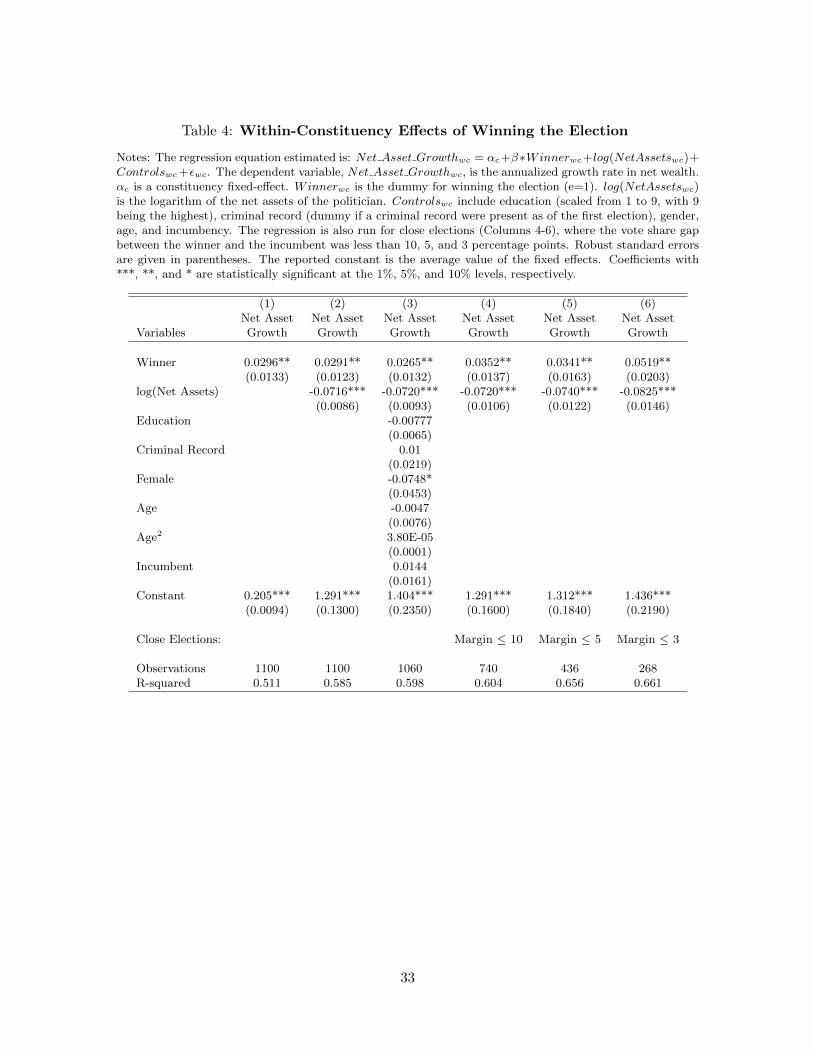
Table 4: Within-Constituency Effects of Winning the Election

Notes: The regression equation estimated is: Net Asset Growthwc = αc+β∗Winnerwc+log(NetAssetswc)+Controlswc +εwc. The dependent variable, Net Asset Growthwc, is the annualized growth rate in net wealth.αc is a constituency fixed-effect. Winnerwc is the dummy for winning the election (e=1). log(NetAssetswc)is the logarithm of the net assets of the politician. Controlswc include education (scaled from 1 to 9, with 9being the highest), criminal record (dummy if a criminal record were present as of the first election), gender,age, and incumbency. The regression is also run for close elections (Columns 4-6), where the vote share gapbetween the winner and the incumbent was less than 10, 5, and 3 percentage points. Robust standard errorsare given in parentheses. The reported constant is the average value of the fixed effects. Coefficients with***, **, and * are statistically significant at the 1%, 5%, and 10% levels, respectively.

(1) (2) (3) (4) (5) (6)Net Asset Net Asset Net Asset Net Asset Net Asset Net Asset

Variables Growth Growth Growth Growth Growth Growth

Winner 0.0296** 0.0291** 0.0265** 0.0352** 0.0341** 0.0519**(0.0133) (0.0123) (0.0132) (0.0137) (0.0163) (0.0203)

log(Net Assets) -0.0716*** -0.0720*** -0.0720*** -0.0740*** -0.0825***(0.0086) (0.0093) (0.0106) (0.0122) (0.0146)

Education -0.00777(0.0065)

Criminal Record 0.01(0.0219)

Female -0.0748*(0.0453)

Age -0.0047(0.0076)

Age2 3.80E-05(0.0001)

Incumbent 0.0144(0.0161)

Constant 0.205*** 1.291*** 1.404*** 1.291*** 1.312*** 1.436***(0.0094) (0.1300) (0.2350) (0.1600) (0.1840) (0.2190)

Close Elections: Margin ≤ 10 Margin ≤ 5 Margin ≤ 3

Observations 1100 1100 1060 740 436 268R-squared 0.511 0.585 0.598 0.604 0.656 0.661

33

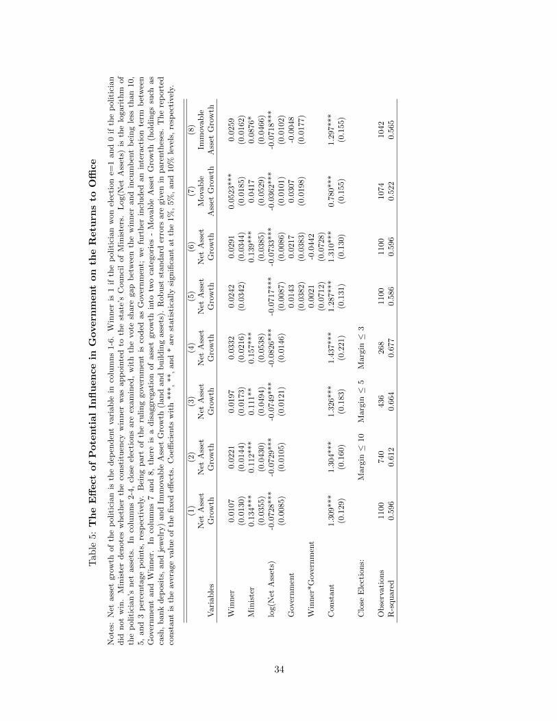
Tab

le5:

Th

eE

ffect

of

Pote

nti

al

Infl

uence

inG

overn

ment

on

the

Retu

rns

toO

ffice

Note

s:N

etass

etgro

wth

of

the

politi

cian

isth

edep

enden

tva

riable

inco

lum

ns

1-6

.W

inner

is1

ifth

ep

oliti

cian

won

elec

tion

e=1

and

0if

the

politi

cian

did

not

win

.M

inis

ter

den

ote

sw

het

her

the

const

ituen

cyw

inner

was

app

oin

ted

toth

est

ate

’sC

ounci

lof

Min

iste

rs.

Log(N

etA

sset

s)is

the

logari

thm

of

the

politi

cian’s

net

ass

ets.

Inco

lum

ns

2-4

,cl

ose

elec

tions

are

exam

ined

,w

ith

the

vote

share

gap

bet

wee

nth

ew

inner

and

incu

mb

ent

bei

ng

less

than

10,

5,

and

3p

erce

nta

ge

poin

ts,

resp

ecti

vel

y.B

eing

part

of

the

ruling

gov

ernm

ent

isco

ded

as

Gov

ernm

ent;

we

furt

her

incl

uded

an

inte

ract

ion

term

bet

wee

nG

over

nm

ent

and

Win

ner

.In

colu

mns

7and

8,

ther

eis

adis

aggre

gati

on

of

ass

etgro

wth

into

two

cate

gori

es-

Mov

able

Ass

etG

row

th(h

old

ings

such

as

cash

,bank

dep

osi

ts,

and

jew

elry

)and

Imm

ovable

Ass

etG

row

th(l

and

and

buildin

gass

ets)

.R

obust

standard

erro

rsare

giv

enin

pare

nth

eses

.T

he

rep

ort

edco

nst

ant

isth

eav

erage

valu

eof

the

fixed

effec

ts.

Coeffi

cien

tsw

ith

***,

**,

and

*are

stati

stic

ally

signifi

cant

at

the

1%

,5%

,and

10%

level

s,re

spec

tivel

y.

(1)

(2)

(3)

(4)

(5)

(6)

(7)

(8)

Net

Ass

etN

etA

sset

Net

Ass

etN

etA

sset

Net

Ass

etN

etA

sset

Mov

able

Imm

ovable

Vari

able

sG

row

thG

row

thG

row

thG

row

thG

row

thG

row

thA

sset

Gro

wth

Ass

etG

row

th

Win

ner

0.0

107

0.0

221

0.0

197

0.0

332

0.0

242

0.0

291

0.0

523***

0.0

259

(0.0

130)

(0.0

144)

(0.0

173)

(0.0

216)

(0.0

342)

(0.0

344)

(0.0

185)

(0.0

162)

Min

iste

r0.1

34***

0.1

12***

0.1

11**

0.1

57***

0.1

39***

0.0

417

0.0

876*

(0.0

355)

(0.0

430)

(0.0

494)

(0.0

538)

(0.0

385)

(0.0

529)

(0.0

466)

log(N

etA

sset

s)-0

.0728***

-0.0

729***

-0.0

749***

-0.0

826***

-0.0

717***

-0.0

733***

-0.0

362***

-0.0

718***

(0.0

085)

(0.0

105)

(0.0

121)

(0.0

146)

(0.0

087)

(0.0

086)

(0.0

101)

(0.0

102)

Gov

ernm

ent

0.0

143

0.0

217

0.0

307

-0.0

048

(0.0

382)

(0.0

383)

(0.0

198)

(0.0

177)

Win

ner

*G

over

nm

ent

0.0

021

-0.0

442

(0.0

712)

(0.0

728)

Const

ant

1.3

09***

1.3

04***

1.3

26***

1.4

37***

1.2

87***

1.3

10***

0.7

80***

1.2

97***

(0.1

29)

(0.1

60)

(0.1

83)

(0.2

21)

(0.1

31)

(0.1

30)

(0.1

55)

(0.1

55)

Clo

seE

lect

ions:

Marg

in≤

10

Marg

in≤

5M

arg

in≤

3

Obse

rvati

ons

1100

740

436

268

1100

1100

1074

1042

R-s

quare

d0.5

96

0.6

12

0.6

64

0.6

77

0.5

86

0.5

96

0.5

22

0.5

65

34

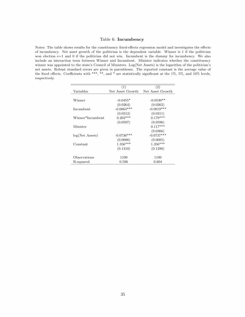
Table 6: Incumbency

Notes: The table shows results for the constituency fixed-effects regression model and investigates the effectsof incumbency. Net asset growth of the politician is the dependent variable. Winner is 1 if the politicianwon election e=1 and 0 if the politician did not win. Incumbent is the dummy for incumbency. We alsoinclude an interaction term between Winner and Incumbent. Minister indicates whether the constituencywinner was appointed to the state’s Council of Ministers. Log(Net Assets) is the logarithm of the politician’snet assets. Robust standard errors are given in parentheses. The reported constant is the average value ofthe fixed effects. Coefficients with ***, **, and * are statistically significant at the 1%, 5%, and 10% levels,respectively.

(1) (2)Variables Net Asset Growth Net Asset Growth

Winner -0.0455* -0.0530**(0.0264) (0.0262)

Incumbent -0.0864*** -0.0819***(0.0312) (0.0311)

Winner*Incumbent 0.203*** 0.179***(0.0597) (0.0596)

Minister 0.117***(0.0366)

log(Net Assets) -0.0736*** -0.0737***(0.0086) (0.0085)

Constant 1.356*** 1.356***(0.1310) (0.1290)

Observations 1100 1100R-squared 0.596 0.604

35

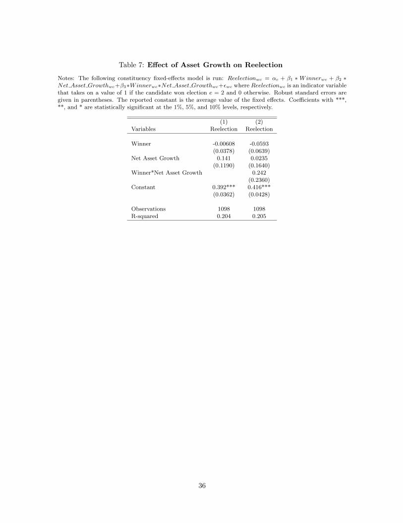
Table 7: Effect of Asset Growth on Reelection

Notes: The following constituency fixed-effects model is run: Reelectionwc = αc + β1 ∗ Winnerwc + β2 ∗Net Asset Growthwc+β3∗Winnerwc∗Net Asset Growthwc+εwc where Reelectionwc is an indicator variablethat takes on a value of 1 if the candidate won election e = 2 and 0 otherwise. Robust standard errors aregiven in parentheses. The reported constant is the average value of the fixed effects. Coefficients with ***,**, and * are statistically significant at the 1%, 5%, and 10% levels, respectively.

(1) (2)Variables Reelection Reelection

Winner -0.00608 -0.0593(0.0378) (0.0639)

Net Asset Growth 0.141 0.0235(0.1190) (0.1640)

Winner*Net Asset Growth 0.242(0.2360)

Constant 0.392*** 0.416***(0.0362) (0.0428)

Observations 1098 1098R-squared 0.204 0.205

36

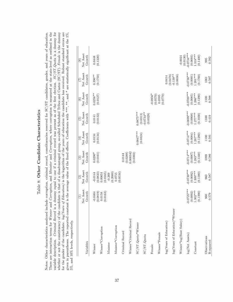
Tab

le8:

Oth

er

Can

did

ate

Ch

ara

cte

rist

ics

Note

s:O

ther

chara

cter

isti

csanaly

zed

incl

ude

corr

upti

on,

crim

inal

reco

rd,

const

ituen

cies

rese

rved

for

SC

/ST

candid

ate

s,gen

der

,and

yea

rsof

educa

tion.

Ther

eare

inte

ract

ion

term

sfo

rW

inner

andCorruption

,andMinister

andCorruption

,w

her

eco

rrupti

on

ism

easu

red

at

the

state

-lev

elas

outl

ined

inth

eva

riable

des

crip

tion.CriminalRecord

isa

dum

my

equal

toone

ifa

crim

inal

reco

rdw

as

pre

sent

as

of

the

firs

tel

ecti

on.SC/ST

Quota

isa

dum

my

for

whet

her

or

not

the

const

ituen

cyof

the

candid

ate

isth

at

of

adis

adva

nta

ged

gro

up,

so-c

alled

Sch

edule

dT

rib

esand

Cast

es(S

C/ST

).Fem

ale

isth

edum

my

for

the

gen

der

of

the

candid

ate

.log(Years

ofEducation)

isth

elo

gari

thm

of

the

yea

rsof

educa

tion

the

candid

ate

has

rece

ived

.R

obust

standard

erro

rsare

giv

enin

pare

nth

eses

.T

he

rep

ort

edco

nst

ant

isth

eav

erage

valu

eof

the

fixed

effec

ts.

Coeffi

cien

tsw

ith

***,

**,

and

*are

stati

stic

ally

signifi

cant

at

the

1%

,5%

,and

10%

level

s,re

spec

tivel

y.

(1)

(2)

(3)

(4)

(5)

(6)

(7)

(8)

Net

Ass

etN

etA

sset

Net

Ass

etN

etA

sset

Net

Ass

etN

etA

sset

Net

Ass

etN

etA

sset

Vari

ab

les

Gro

wth

Gro

wth

Gro

wth

Gro

wth

Gro

wth

Gro

wth

Gro

wth

Gro

wth

Win

ner

-0.0

464

-0.0

144

0.0

290*

0.0

134

0.0

141

0.0

256**

0.3

96**

0.0

448

(0.0

819)

(0.0

833)

(0.0

161)

(0.0

134)

(0.0

132)

(0.0

127)

(0.1

750)

(0.1

220)

Win

ner

*C

orr

up

tion

0.0

158

0.0

0651

(0.0

163)

(0.0

165)

Min

iste

r-0

.269

(0.2

660)

Min

iste

r*C

orr

up

tion

0.0

755

(0.0

534)

Cri

min

al

Rec

ord

0.0

144

(0.0

288)

Win

ner

*C

rim

inal

Rec

ord

0.0

00342

(0.0

392)

SC

/S

TQ

uota

*W

inn

er0.0

847***

0.0

875***

(0.0

324)

(0.0

313)

SC

/S

TQ

uota

-0.0

734**

(0.0

329)

Fem

ale

-0.0

956*

(0.0

570)

Win

ner

*F

emale

0.0

595

(0.0

770)

log(Y

ears

of

Ed

uca

tion

)0.0

414

(0.0

478)

log(Y

ears

of

Ed

uca

tion

)*W

inn

er-0

.139**

(0.0

656)

Win

ner

*lo

g(B

ase

Sala

ry)

-0.0

024

(0.0

130)

log(N

etA

sset

s)-0

.0725***

-0.0

730***

-0.0

714***

-0.0

714***

-0.0

699***

-0.0

709***

-0.0

730***

-0.0

734***

(0.0

092)

(0.0

092)

(0.0

087)

(0.0

084)

(0.0

068)

(0.0

085)

(0.0

091)

(0.0

093)

Con

stant

1.3

02***

1.3

09***

1.2

83***

1.2

87***

1.2

77***

1.2

86***

1.2

01***

1.3

18***

(0.1

390)

(0.1

380)

(0.1

340)

(0.1

280)

(0.1

030)

(0.1

290)

(0.1

760)

(0.1

400)

Ob

serv

ati

on

s960

960

1099

1100

1100

1100

1061

995

R-s

qu

are

d0.5

79

0.5

87

0.5

86

0.5

91

0.4

19

0.5

88

0.5

97

0.5

92

37

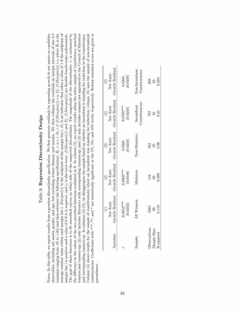
Tab

le9:

Regre

ssio

nD

isconti

nu

ity

Desi

gn

Note

s:In

this

table

,w

ere

port

resu

lts

from

regre

ssio

ndis

conti

nuit

ysp

ecifi

cati

on.

We

firs

tgen

erate

resi

duals

by

regre

ssin

ggro

wth

innet

ass

ets

on

candid

ate

obse

rvable

s,in

cludin

gnet

ass

ets,

gen

der

,and

age,

but

excl

udin

gw

inner

dum

my

and

marg

in.

We

then

collapse

the

resi

duals

on

marg

inin

terv

als

of

size

0.5

(marg

ins

rangin

gfr

om

-25

to+

25)

and

then

esti

mate

the

follow

ing

spec

ifica

tion:R̄

i=α

+τ·D

i+β·f

(Margin

(i))

+η·D

i·f

(Margin

(i))

+ε i

wher

eR̄

iis

the

aver

age

resi

dual

valu

ew

ithin

each

marg

inbin

i,Margin

(i))

isth

em

idp

oin

tof

the

marg

inbin

i,D

iis

an

indic

ato

rth

at

takes

ava

lue

of

1if

the

mid

poin

tof

marg

inbin

iis

posi

tive

and

ava

lue

of

0if

itis

neg

ati

ve,

andε i

isth

eer

ror

term

.f

(Margin

(i))

andD

i·f

(Margin

(i))

are

flex

ible

fourt

h-o

rder

poly

nom

ials

.T

he

goal

of

thes

efu

nct

ions

isto

fit

smooth

edcu

rves

on

eith

ersi

de

of

the

susp

ecte

ddis

conti

nuit

y.T

he

magnit

ude

of

the

dis

conti

nuit

y,τ,

ises

tim

ate

dby

the

diff

eren

cein

the

valu

esof

the

two

smooth

edfu

nct

ions

evalu

ate

dat

0.

Inco

lum

n(1

),w

ere

port

resu

lts

usi

ng

the

enti

resa

mple

of

const

ituen

cym

atc

hed

win

ner

sand

runner

s-up;

(2)

only

incl

udes

Ministers

wit

hco

rres

pondin

gru

nner

s-up,

and

(3)

only

incl

udes

win

ner

snot

app

oin

ted

toth

eC

ounci

lof

Min

iste

rsand

corr

esp

ondin

gru

nner

s-up.

Inco

lum

ns

(4)-

(5),

we

dis

aggre

gate

the

sam

ple

base

don

whet

her

an

incu

mb

ent

isst

andin

gfo

rre

elec

tion

inth

eco

nst

ituen

cy.

Colu

mn

(4)

show

sre

sult

sfo

rth

esa

mple

of

const

ituen

cies

wher

ean

incu

mb

ent

was

standin

gfo

rre

elec

tion;

colu

mn

(5)

use

sth

esa

mple

of

non-i

ncu

mb

ent

const

ituen

cies

.C

oeffi

cien

tsw

ith

***,

**,

and

*are

stati

stic

ally

signifi

cant

at

the

1%

,5%

,and

10%

level

s,re

spec

tivel

y.R

obust

standard

erro

rsare

giv

enin

pare

nth

eses

.

(1)

(2)

(3)

(4)

(5)

Net

Ass

etN

etA

sset

Net

Ass

etN

etA

sset

Net

Ass

etV

ari

able

sG

row

thR

esid

ual

Gro

wth

Res

idual

Gro

wth

Res

idual

Gro

wth

Res

idual

Gro

wth

Res

idual

τ0.0

652***

0.2

869***

0.0

265

0.0

799***

0.0

283

(0.0

233)

(0.0

546)

(0.0

234)

(0.0

250)

(0.0

358)

Sam

ple

:A

llW

inner

sM

inis

ters

Non-M

inis

ters

Incu

mb

ent

Non-I

ncu

mb

ent

Const

ituen

cies

Const

ituen

cies

Obse

rvati

ons

1065

144

921

797

268

Marg

inB

ins

98

68

95

91

83

R-s

quare

d0.1

19

0.3

99

0.0

60.2

10.2

84

38

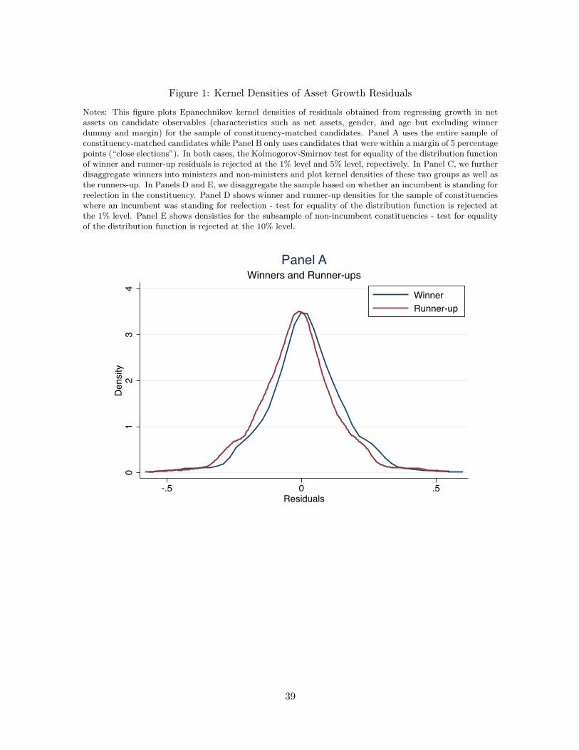
Figure 1: Kernel Densities of Asset Growth Residuals

Notes: This figure plots Epanechnikov kernel densities of residuals obtained from regressing growth in netassets on candidate observables (characteristics such as net assets, gender, and age but excluding winnerdummy and margin) for the sample of constituency-matched candidates. Panel A uses the entire sample ofconstituency-matched candidates while Panel B only uses candidates that were within a margin of 5 percentagepoints (“close elections”). In both cases, the Kolmogorov-Smirnov test for equality of the distribution functionof winner and runner-up residuals is rejected at the 1% level and 5% level, repectively. In Panel C, we furtherdisaggregate winners into ministers and non-ministers and plot kernel densities of these two groups as well asthe runners-up. In Panels D and E, we disaggregate the sample based on whether an incumbent is standing forreelection in the constituency. Panel D shows winner and runner-up densities for the sample of constituencieswhere an incumbent was standing for reelection - test for equality of the distribution function is rejected atthe 1% level. Panel E shows densisties for the subsample of non-incumbent constituencies - test for equalityof the distribution function is rejected at the 10% level.

01

23

4D

ensi

ty

-.5 0 .5Residuals

WinnerRunner-up

Winners and Runner-upsPanel A

39

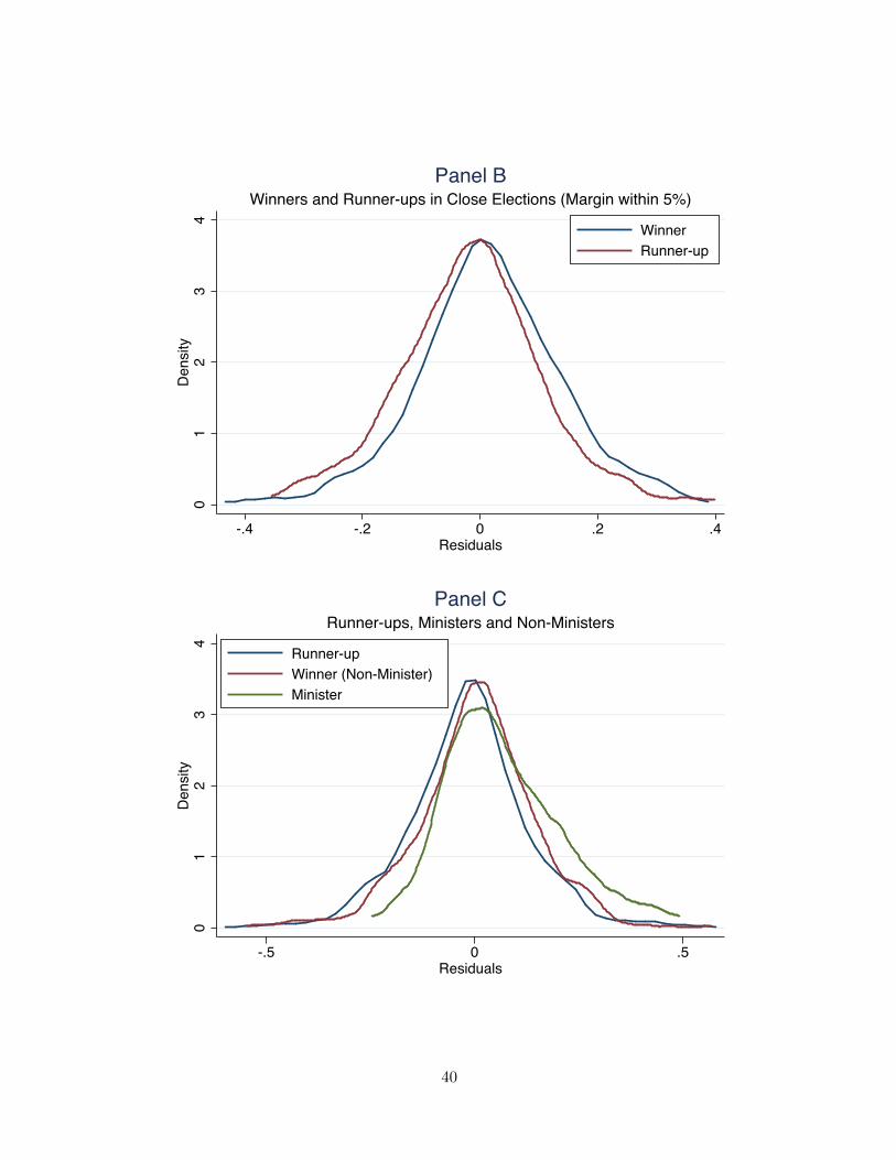
01

23

4D

ensi

ty

-.4 -.2 0 .2 .4Residuals

WinnerRunner-up

Winners and Runner-ups in Close Elections (Margin within 5%)Panel B

01

23

4D

ensi

ty

-.5 0 .5Residuals

Runner-upWinner (Non-Minister)Minister

Runner-ups, Ministers and Non-MinistersPanel C

40

01

23

4D

ensi

ty

-.5 0 .5Residuals

WinnerRunner-up

Constituencies with Incumbent standing for reelectionPanel D

01

23

Den

sity

-.5 0 .5Residuals

WinnerRunner-up

Constituencies without Incumbent standing for reelectionPanel E

41

Figure 2: Regression Discontinuity Design

Notes: This figure investigates residuals obtained from regressing growth in net assets on candidate observables(characteristics such as net assets, gender, age and incumbency but excluding winner dummy and margin) asa function of winning margin for the sample of constituency-matched candidates. We first collapse residualson margin intervals of size 0.5 (margins ranging from -25 to +25) and then estimate the following equation:R̄i = α+ τ ·Di + β · f(Margin(i)) + η ·Di · f(Margin(i)) + εi where R̄i is the average residual value withineach margin bin i, Margin(i)) is the midpoint of the margin bin i, Di is an indicator that takes a valueof 1 if the midpoint of margin bin i is positive and a value of 0 if it is negative, and εi is the error term.f(Margin(i)) and Di · f(Margin(i)) are flexible fourth-order polynomials. Panel A shows results using thesample of all winners sand runners-up; Panel B only includes Ministers with corresponding Runners-up; PanelC only includes winners that were not appointed to the Council of Ministers with corresponding Runners-up.In Panels D and E, we disaggregate the sample based on whether an incumbent is standing for reelection inthe constituency. Panel D shows results for the sample of constituencies where an incumbent was standingfor reelection; Panel E shows the subsample of non-incumbent constituencies.

-.2-.1

0.1

.2R

esid

uals

-20 0 20Margin Bin

Runner-ups and WinnersPanel A

42

-.4-.2

0.2

.4R

esid

uals

-20 0 20Margin Bin

Runner-ups and MinistersPanel B

-.20

.2R

esid

uals

-30 -20 -10 0 10 20Margin Bin

Runner-ups and Non-MinistersPanel C

43

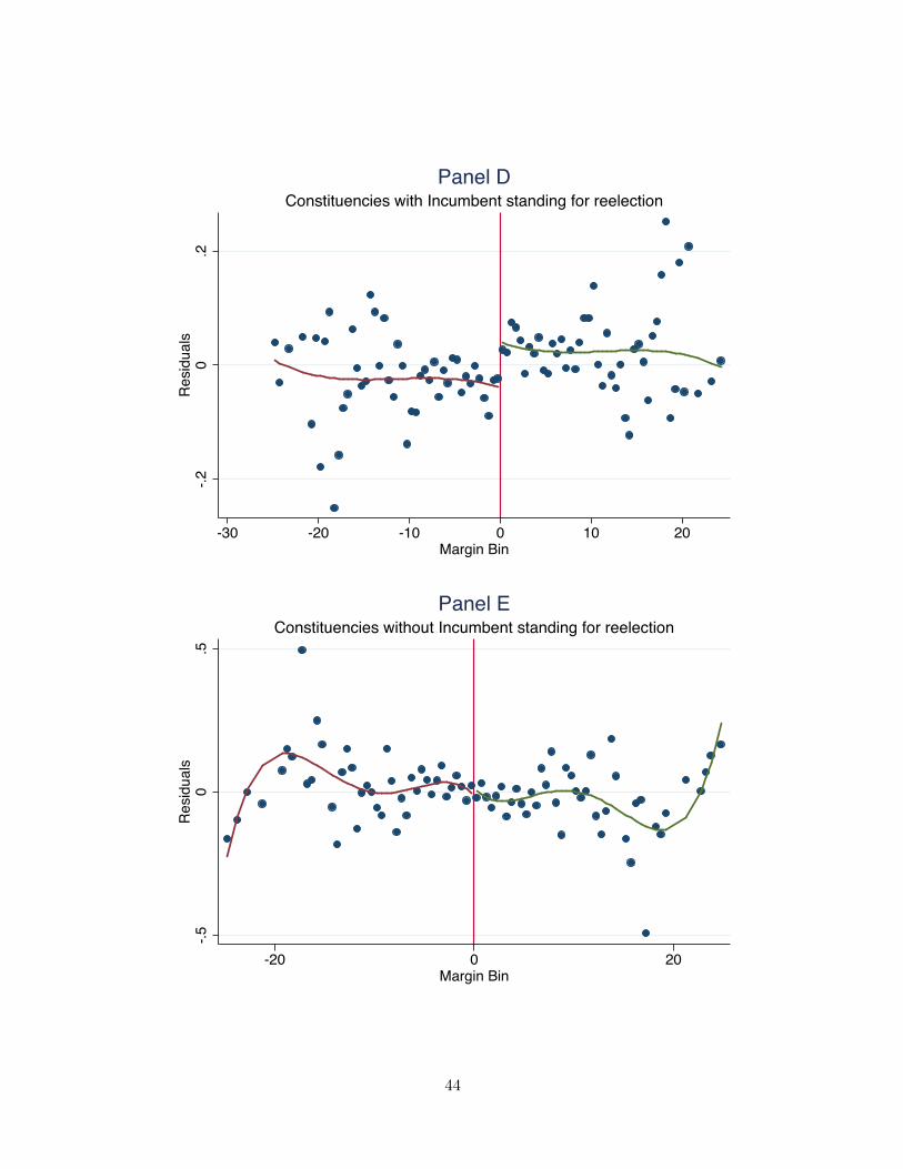
-.20

.2R

esid

uals

-30 -20 -10 0 10 20Margin Bin

Constituencies with Incumbent standing for reelectionPanel D

-.50

.5R

esid

uals

-20 0 20Margin Bin

Constituencies without Incumbent standing for reelectionPanel E

44

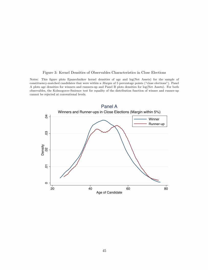
Figure 3: Kernel Densities of Observables Characteristics in Close Elections

Notes: This figure plots Epanechnikov kernel densities of age and log(Net Assets) for the sample ofconstituency-matched candidates that were within a Margin of 5 percentage points (“close elections”). PanelA plots age densities for winners and runners-up and Panel B plots densities for log(Net Assets). For bothobservables, the Kolmogorov-Smirnov test for equality of the distribution function of winner and runner-upcannot be rejected at conventional levels.

0.0

1.0

2.0

3.0

4D

ensi

ty

20 40 60 80Age of Candidate

WinnerRunner-up

Winners and Runner-ups in Close Elections (Margin within 5%)Panel A

45

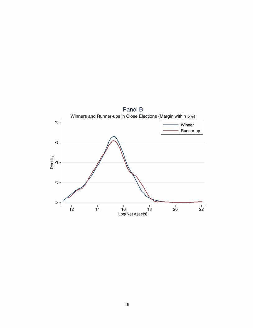
0.1

.2.3

.4D

ensi

ty

12 14 16 18 20 22Log(Net Assets)

WinnerRunner-up

Winners and Runner-ups in Close Elections (Margin within 5%)Panel B

46

Figure 4: Recontesting of Candidates

Notes: We investigate recontesting decisions for winners and runners-up. In a first stage we obtain residualsfrom regressing a binary recontesting dummy on candidate observables (characteristics such as age, gender,incumbency but excluding winner dummy and margin) and constituency fixed effects. Residuals are thencollapsed into margin bins and a polynomial is fitted to the data. In Panel A, we show results for the fullsample (5246 candidates), indicating a significant jump in recontesting around the winning threshold (pointestimate of 0.1328 with a t-statistic of 6.41). In Panel B, we show results for for the subsample of seasonedpoliticians (322 candidates) - no jump in recontesting can be detected around the threshold. In Panel C,we analyze net asset growth residuals for the subsample of seasoned politicians. The point estimate of thediscontinuity is 0.1206 and significant at the 5% level (t-statistic of 2.19).

-.4-.2

0.2

Res

idua

ls

-20 -10 0 10 20Margin Bin

Recontesting Probability ResidualsPanel A

47

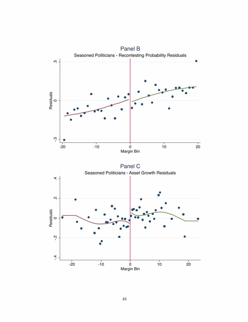
-.50

.5R

esid

uals

-20 -10 0 10 20Margin Bin

Seasoned Politicians - Recontesting Probability ResidualsPanel B

-.4-.2

0.2

.4R

esid

uals

-20 -10 0 10 20Margin Bin

Seasoned Politicians - Asset Growth ResidualsPanel C

48