prince william sound recovery rate analysis - … · prince william sound recovery rate analysis a...

Prince William Sound Recovery Rate Analysis

A Report to:

Prince William Sound Regional Citizens’ Advisory Council

October 27, 2008

Prepared by:

Censum Northwest, LLC P.O. Box 12082

Olympia, WA 98508

www.censumnw.com

700.431.081027.PWSRecovRate

The opinions expressed in this PWSRCAC commissioned report are not necessarily those of PWSRCAC.

Executive Summary

This study was developed in response to Prince William Sound RCAC’s Request for Proposal (RFP #760). The RFP identified three interrelated tasks; each was addressed in this study:

1) This study compares response planning concepts of encounter rates with recovery rates.

2) This study evaluates the relative effectiveness of Current Buster Task Forces and U/J configurations for the Near Shore response.

3) Given the tactics described in the 2007 SERVS Technical Manual, this study evaluated the overall capacity to recover oil within 72 hours.

This study analyzed basic planning schemes against a specific set of scenario factors and calculated recovery rates to establish a range outcome. Additionally, to further broaden the understanding of recovery rates, this study provides a brief qualitative analysis predicting outcomes against a broader range of scenario factors. As the principal methodology, this study utilized ASTM F1780 (2002) A Standard Guide for Estimating Oil Spill Recovery System Effectiveness. ASTM designed this standard to account for deficiencies in the EDRC approach. To make the analysis less generic and more realistic the study relied upon spill trajectory and weathering models when developing scenario factors. How do Current Buster Task Forces compare with U/J Task Forces? Current Buster System Task Forces likely will far out pace U and J boom configuration task forces. In scenarios where slicks are widely spread or discontinuous, differences between the two systems will be especially pronounced, where one Current Buster Task force may be worth 5 U/J Task Forces. Current Buster advantages include: a higher throughput efficiency, higher encounter rate, higher recovery efficiency, greater ability to deal with choppy water, ability to operate in high current areas such as "bottle neck pinch points", greater maneuverability, and the advantage of an inherent storage system (allows for more continuous operation). We believe debris handling is the principal disadvantage of Current Busters. What is the capacity of the Near Shore and Open Water Response? This study considered instantaneous and continuous release spill scenarios. More specifically, this study considered:

• 300,000 barrels released instantly • 300,000 barrels released constantly over the first day, 165,000 barrels released

constantly over the second day, and 165,000 barrels released constantly over the third day.

• 300,000 barrels released instantly, 165,000 barrels released constantly over the second day, and 165,000 barrels released constantly over the third day.

As requested by RCAC the study considered a variety of response parameters for each type of scenario. Over all, our analysis shows that encounter rate is likely to be a



significant limitation when large volumes of oil are released rapidly. Since these spills spread quickly over a large geographic area, there is little opportunity for extremely high encounter rates. Continuous release spills on the other hand, afford the opportunity to capture oil before it spreads out over a large geographic area. The following table summarizes the scenarios analyzed and projected outcomes:

Scenario Description Projected Outcome BBLS Recovered = 22,062

300,000 barrel instantaneous release

Central Prince William Sound10 knot winds, easterly and southerly No LEL concern

Scenario #2

Description Projected Outcome BBLS Recovered = 246,980

Central Prince William Sound300,000 barrels continuously released over first 24 hours, additional 330,000 barrels continuously released between hour 24 and hour 72 Central Prince William Sound10 knot easterly windsLEL concerns near release

Scenario #3


300,000 barrels instantaneously released, 330,000 barrels continuously released between hour 24 and hour 72 Central Prince William Sound10 knot easterly windsLEL concern for continuous release

Scenario #5

Description Projected Outcome BBLS Recovered = <1,000

Hinchinbrook Entrance 300,000 barrels instantaneous release 12 knot winds easterly winds No LEL concern

Scenario #4

Description Projected Outcome BBLS Recovered = <10,000 Hinchinbrook Entrance

300,000 barrels continuously released over first 24 hours, additional 330,000 barrels continuously released between hour 24 and hour 72 12 knot winds easterly windsNo LEL concern

#1:



How could response to instantaneous release scenarios be improved? RCAC asked for advice regarding what could potentially improve the ability to deal with instantaneous releases. Although, developing detailed alternative response schemes exceeds the scope of this study. The following measures should be considered:

• Improve response time and drop the EDRC Approach: Contrary to what is suggested by the EDRC approach, improving response time will improve performance. Planners should anticipate that recovery rates will change through time and plan accordingly. The highest recovery rates come early, before slicks spread widely, break into patches, or impact adjacent shorelines.

• Encourage development of assessment tools and technology: On-water

recovery, to be effective, largely depends upon the ability to steer recovery systems into the highest concentrations of oil. During periods of good visibility, visual observations from aircraft can be used to effectively direct recovery systems toward the highest apparent concentrations of oil. Periods of darkness preclude the ability to visually observe oil. The existing capacity could be significantly improved through improvements in real time mapping and data transmission from these aircraft to recovery systems. Improvements, above and beyond IR technology, in the ability to detect and track the highest concentrations of oil, especially during darkness, will lead to better performance. Consider investment in remote sensory technology devices and associated mapping software, especially scanning laser fluorosensors. During daylight, improvements in assessment technology could dramatically help improve results since visual observations are generally unreliable at quantifying black oil. The “magic bullet” of oil spill response, where the greatest possible improvement can be made, may be to develop technology to effectively measure slick thickness remotely. Consider continuing support research for improvements in technology that can detect, measure, and map oil spills remotely.

• Anticipate a large slick area: The existing Prince William Sound response composition is geared especially well towards addressing a thick layer of oil. A separate response scheme may be needed where a large number of smaller systems may achieve better results, given spills spread over several square miles.

• Emphasize recovery systems with high encounter speed, high recovery

efficiency, and many more smaller agile storage devices: Improving encounter speed and effective swath widths improves the potential for encountering oil, consider increasing the use of high encounter speed technology such as Current Buster task forces. There are two principal ways to build up the existing response capacity to better deal with instantaneous release scenarios. Either invest in more large recovery systems or invest in many smaller recovery systems. Since dealing with large volumes of recovered oil presents a difficult challenge, some might argue that large systems are the way to go, and that it is



just a matter of directing the oil to these barges mounted with recovery devices. Large-barge recovery systems can effectively utilize high rate, low efficiency skimmers since they are more likely able to effectively decant. The problem with this approach is that as ever-increasing swath widths are required (perhaps thousands of feet), frequent failure is almost certain due to debris, maneuverability issues, especially toward preventing entrainment.

The other principal alternative is to invest in many smaller recovery systems. High efficiency, high encounter speed, but still with significant swath width recovery systems will maximize this approach. High efficiency means less need for storage and high encounter speeds with significant swath width means high encounter rates. A current buster task force with a swath width of 73 feet could theoretically encounter thousands of barrels in a day at high recovery efficiency. Faced with a relatively spread out slick of 0.1 mm thickness a current buster system might still recovery 100 barrels per hour. A system mounted with 1000 barrels of storage capacity could recover up to 1000 barrels in a day, with very little water. Additional current buster or ocean buster systems would be needed to meet this demand as well as towable storage dracones. 50 such teams would be would be needed to recover 50,000 barrels per day.

• Expand use of In Situ Burning: The number of complete recovery systems

required to make up the lack of encounter rate may not be practical. A hundred or more collection systems, each with several small barges or bladders, might be needed. For many scenarios, in-situ burning may be the only practical solution. Consider burning, not just within the collection apex, but as part of a more complex high encounter speed system. Such a system could extend the operating window.

• Anticipate rapid shoreline grounding of oil: Consider additional investment in

the response capacity to stabilize high volumes of temporarily stranded oil. High volume plans (such as the use of highly mobile mechanized shoreline methods) should be developed for such scenarios, bearing in mind that near shore skimming systems may not be appropriate for exposed environments.



Table of Contents Executive Summary ............................................................................................... i Table of Contents ................................................................................................... v List of Figures ......................................................................................................... vi List of Tables .......................................................................................................... vii Chapter 1: Introduction and Scope ....................................................................... 1

Background ...................................................................................... 2 Relationship Between Encounter Rate

and Recovery Rate ................................................................ 2 Additional works related to this report ............................................... 7

Chapter 2: Methodology Guides and Models ........................................................ 9

Methodology Guides ......................................................................... 9 Spill Models ....................................................................................... 9

Chapter 3: Recovery System Effectiveness Comparison of U/J Boom with Current Buster Configuration ....................................... 10

Applying ASTM F1780-97 (2002) to Estimate Recovery System Effectiveness for Comparison of U/J Boom with Current Buster Configuration .............................................................. 12

Results of Analysis Comparing Recovery System Effectiveness of Current Buster and U and J Boom Configurations Task Forces. …………………………. 25

Chapter 4: Determination of Recovery Rates for

Prince William Sound Recovery Systems .......................................... 28 Applying ASTM F1780-97 (2002) to Estimate

Recovery System Effectiveness............................................... 34 Determination of Recovery Rates for Prince

William Sound Recovery Systems Results ............................ 52 Results Summary .............................................................................. 63 Chapter 4 Discussion ........................................................................ 64 Overall Discussion ............................................................................ 66

Appendix 1: Definitions Appendix 2: Scenario Details Appendix 3: Anvil Comparison Bibliography



List of Figures Figure 3-1 U Module Strike Team From the 2002 Prince William Sound Tanker Oil Discharge Prevention and Contingency Plan ..................................................................... 10 Figure 3-2 J Module, from 2007 SERVS Technical Manual ................................ 11 Figure 3-3 Current Buster Configuration from 2007 SERVS Technical Manual ............................................................................ 11 Figure 3-4 Theoretical Fast Current Bottleneck ................................................... 15 Figure 3-5 Patchy “Free-Oil” From 2007 SERVS Technical Manual Near-Shore Tactics ............................................. 23 Figure 4-1 Illustration, Tactic Purpose and Description of Task Forces 1-4A from the 2007 SERVS Technical Manual ............................................................................. 29 Figure 4-2 Illustration, Tactic Purpose and Description of Task Force 5 from the 2007 SERVS Technical Manual ............................................................................. 30 Figure 4-3 Tactic Purpose and Description of near-shore Task Forces 1-4 from the 2007 SERVS Technical Manual ............................................................................. 31 Figure 4-4 Spill Scenario Start Sites from Hinchinbrook Entrance and Central Prince William Sound. .................................... 32 Figure 4-5 Central Prince William Sound 72-Hour Spill Trajectory ...................... 36 Figure 4-6 Central Prince William Sound Continuous Release Scenario at Hour 6. ......................................................................... 37 Figure 4-7 ADIOS II Modeled Changes in Density, Emulsification, Evaporation, and Viscosity .............................................................. 38 Figure 4-8 TransRec Task Force Operating in a Non-Static Mode, SERVS Exercise, August 23, 2007 .................................................. 45 Figure 4-9 An Estimation of Oil Recovery Potential by Open Water Task Forces (1-5), given a 300,000 barrel instantaneous release and 0.5 knot encounter speed limitation ................................................................................ 53 Figure 4-8 An Estimation of Oil Recovery Potential by Near Shore Task Forces (1-4), given a 300,000 barrel instantaneous release and 0.5 knot encounter speed limitation for U/J Task Forces ........................................................... 54 Figure 4-9 An estimation of Oil Recovery Potential by Open Water and Near Shore Task Forces, given a 300,000 barrel instantaneous release and 0.5 knot encounter speed limitation ........................................................................................... 54 Figure 4-10 An Estimation of Oil Recovery Potential by Open Water Task Forces (1-5), given a 300,000 barrel instantaneous release and 0.7 knot encounter speed limitation ............................................................................... 56 Figure 4-11 An estimation of oil recovery potential by Open Water



and Near Shore Task Forces, given a 300,000 barrel instantaneous release and 0.7 knot encounter speed limitation .......................................................................................... 56 Figure 4-12 An Estimation of Oil Recovery Potential by Open Water Task Forces (1-5), given spill rates of 300,000 barrels per day on day 1, and 165,000 barrels per day on day 2 and on day 3 ..................................................................... 58 Figure 4-13 An Estimation of Oil Recovery Potential by Open Water and Near Shore Task Forces, given spill rates of 300,000 barrels per day on day 1, and 165,000 barrels per day on day 2 and on day 3 ........................................................ 58 Figure 4-14 Hinchinbrook Entrance Instantaneous Release, slick area at 72 hours (GNOME Trajectory) ..................................... 60 Figure 4-15 PWS-NS-1E from the 2007 SERVS Manual ....................................... 61 Figure 4-16 Continuous Release scenarios from Hinchinbrook Entrance .............. 62 Figure 4-19 Barrels Recovered .............................................................................. 65

List of Tables

Table 1-1 Comparison of Encounter Rates for Spills 0.1 mm thick with De-Rated Oil Recovery Rates ........................................ 6 Table 1-2 Comparison of Encounter Rates for Spills 1.0 mm thick emulsion with De-Rated Oil Recovery Rates ......................... 7 Table 3-1 Current Buster Performance at 2.0, 3.0 and 3.5 Knots ..................... 19 Table 3-2 Relative Advantages of Current Buster versus U/J Boom System ............................................................... 25 Table 3-3 Scenario Summary. Limiting factors: Encounter Rate (ER), Though-put Efficiency (TE), Nameplate Recovery Rate, and Recovery ................................................................................. 26 Table 4-1 Instantaneous Release Emulsion Thickness ..................................... 39 Table 4-2 Estimate of Volume of a 300,000 barrel Spill Recoverable within 72 Hours .......................................................... 53 Table 4-3 Barrels Oil Recovered by Task Forces limited by 0.7 knot Encounter Speed ..................................................................... 55 Table 4-4 Barrels of Oil Recovered by Task Forces, given a continually released spill ..................................................... 57



1. Introduction and Scope This study was developed in response to Prince William Sound RCAC’s Request for Proposal (RFP) Number 760 (See Appendix 2). Two important considerations leading to the development of this report:

1) State of Alaska regulations as well as the Prince William Sound Tanker Oil Discharge Prevention and Contingency Plan require a response capability sufficient to meet a Response Planning Standard (RPS) of containing and cleaning-up 300,000 barrels of oil within a 72 hour time frame. Some may wonder whether this capability actually exists.

2) In 2006, Alaska approved the use of Current Buster recovery systems as an

improvement to the previous response capability for both near-shore and open-water task forces. This change brought about concerns regarding the ability of the Current Buster Systems to recover oil at rates equal to oil recovery systems previously relied upon.

In this report we estimate potential recovery system effectiveness for both open and near shore response, as defined in the SERVS Technical Manual. Specifically, in this report, we respond to the following tasks prescribed by the Prince William Sound RCAC RFP:

1) When considering encounter rate, how does the recovery rate compare between

Current Buster Task Forces with “U” and “J” boom configurations for near-shore responses?

2) When considering encounter rate, given a 300,000 barrel spill and maximum

dispersion1, what is the potential to recover spilled oil in 72 hours for both the near-shore and open water task forces?

1 Although the RFP called for “maximum dispersion” or slick spreading, this study relied on more favorable scenario assumptions, since maximum dispersion occurs during storms events when mechanical recovery is infeasible. Based on slick behavior following the Exxon Valdez, expect the slick to spread out ten times faster during storm events (2007interview with NOAA Spill Modeler Watabayashi).



1.1. Background

1.1.1. Relationship Between Encounter Rate and Recovery Rate As background for this report Prince William RCAC requested a full description of the relationship between recovery rate and encounter rate. The relationship is self-evident:

Spilled oil must be encountered by recovery systems before recovery of oil is possible.

Ignoring this relationship does a great disservice to the usefulness of planning efforts. Yet, this is precisely what happens when planners assign recovery systems a “De-Rated Recovery Rate” or “Effective Daily Recovery Capacity”, since this approach neglects to take into account limitations posed by encounter rate. “De-Rating” often suggests the potential for unrealistically high recovery rates and may fail to take into account logistical difficulties posed by continuously dealing with the recovered oil and oily water. EDRC assumes that effectiveness at hour one is the same as at hour 100, very unlikely.

1.1.1.1. A few important but potentially confusing definitions related to recovery rates2:

Effective Daily Recovery Capacity (EDRC) approach - The product of the skim units “Nameplate” capacity with an efficiency factor. The SERVS manual refers to this product as the “De-Rated Oil Recovery Rate”. Nameplate Capacity - The manufacturer’s suggested maximum pump rate for each skim unit. Although ASTM is developing a standard, currently the rate reported is highly subjective. Oil Spill Recovery SystemASTM – A combination of devices that operate together to recover spilled oil; the system would include some or all of the following components:

Containment boom. Skimmer(s). Support vessels to deploy and operate the boom and skimmer(s). Discharge/transfer pumps. Oil/water separator. Temporary storage devices. Shore based storage/disposal.

2 This study provides a more comprehensive listing of definitions in Appendix



Recovery RateASTM – The appropriate recovery rate must be determined for the skimming unit based on the operating conditions specified in the spill scenario. The recovery rate should reflect realistic expectations of performance with regard to the slick thickness and viscosity as well as the specified environmental conditions, all of which may vary with time. Encounter RateASTM The encounter rate of the recovery system is a prime consideration in evaluating performance. The encounter rate is the rate (m3/h) at which the system encounters an oil slick. The encounter rate includes three components: sweep width, encounter speed, and oil slick thickness. Thoughput EfficiencyMEC-The percentage of oil encountered that is recovered. A recovery system’s throughput efficiency frequently decreases with encounter speed and wave chop because of boom failure. Recovery EfficiencyASTM – A skimmer will generally recover free water along with the recovered oil. The amount of water recovered will affect the relative efficiency of a skimmer system because the total fluid volume must be handled by the transfer, storage, and disposal systems. In order to estimate the amount of total fluids that must be handled, the recovery efficiency of the skimming system must be known for the operating conditions expected. As with the recovery rate, the recovery efficiency may vary with the slick conditions and the environmental conditions, and should be estimated based on test data if available. Although not discussed in the ASTM standard, a related term is 'throughput efficiency”, which is the percent of oil encountered that is recovered Recovery System EffectivenessASTM – The volume of oil that is removed from the environment by a given recovery system in a given recovery period. The RFP calls for “recovery rate” over 72 hours. Since for most scenarios recovery rate changes hourly as slicks continually spread, in this report we use the ASTM term “Recovery System Effectiveness” as a more technically correct terminology.

1.1.1.2. Studies or works pointing out differences between encounter rate and recovery rate

US Coast Guards Caps Review (1999)3: Encounter rate and access to continuous storage are principal limitations to on water recovery. Since EDRC assumes neither limitation affects recovery rate, it represents a "best case" estimate.

3 U.S. Coast Guard, “Response Plan Equipment Caps Review,” COMDT CG-5431.

http://www.uscg.mil/VRP/reg/capsreview.html



The World Catalog of Oil Spill Response Products (2005): “Oil released at sea spreads over a broad area in a short time…. In short, oil spill contingency plans that do not consider encounter rate (use of EDRC) for typical scenarios are not dealing with the problem. NOAA’s Mechanical Equipment Calculator MEC: As described in the Proceedings of the International Oil Spill Conference (Allen,1999)4. “EDRC (or derating factors) can be misleading as they only reflect a skimmer manufacturer’s nameplate calculation the system’s skimming or pumping. By multiplying the hourly recovery capacity by 24 hours, and then using 20% (or higher in some cases) of that value, a predicted daily recovery potential is established that remains the same day after day, regardless of 1) the actual time on location each day, 2) the time required to fill onboard storage and offload recovered oil and water, and 3) the nature and condition of the oil being encountered.” MEC was specifically designed to account for deficiencies of the EDRC approach. ASTM F1780-97 (2002): ASTM specifically designed this standard to account for deficiencies in the EDRC approach.

1.1.1.3. Field data describing differences between encounter rate and recovery rate

Few if any spill responses achieve an EDRC level of effectiveness. Because the relationship is so intangible, few if any studies have been conducted. At the Exxon Valdez spill and more recently at the Cosco Busan spill, EDRC vastly over-stated actual recovery rates. At the Cosco Busan spill encounter rate limitations precluded the possibility of achieving the EDRC rate:

• Over 60,000 barrels per day EDRC on scene on day 1 • Only 170 barrels of oil actually recovered during day 1.

At the Exxon Valdez spill integral storage limitations (at least initially) precluded responders from achieving EDRC rates:

• 48,000 barrels per day EDRC on scene on day 1 • Only 1200 barrels of oil actual recovered during day 1.

4 Allen, A. et al. 1999, “Assessment of Potential Oil Spill Recovery Capabilities”. 1999 Proceedings of the

International Oil Spill Conference. Seattle, Washington.



1.1.1.4. Experimental data describing differences between

encounter rate and recovery rate A lack of experimental data should not be a surprise, given the inherent nature of the relationship and difficulties posed by experimental design. According to OHMSETT5, the national testing center for oil spill response equipment, facility tests as currently designed do not look at encounter rate or the relationship between encounter rate and recovery rate. Some tests do look at slick thickness as it relates to recovery efficiency. The general design used for evaluating skimmer performance does not take into account the effect of increasing or decreasing encounter rates (ASTM F631 and F808). OHMSETT tests many different types of response equipment, but generally, does not simultaneously assess the efficiency of an entire system (boom, skimmer, swath width, etc). Testing typically consists of 100 feet of firmly stabilized contractor boom with a 30 foot swath width moved through a test pool with consistent and predictable environmental conditions such as speed, current, winds, and wave height. Skimmers are then placed at the apex of the containment configuration and their effectiveness is measured. Storage limitations and design are also not considered in these tests. This is an idealized set up and does not capture the likely effectiveness of entire recovery systems. To some extent the Current Buster set up has been more thoroughly tested since it comes complete as a single packaged tested recovery system.

1.1.1.5. What differences can be numerically inferred between encounter rate and recovery rate

NOAA’s Mechanical Equipment Calculator and the ASTM F1780-97 (2002) provide methods to numerically describe the relationship between encounter rate and recovery rate. The encounter rate for any system is the product of the average slick thickness, the swath width, and the transit speed. A number of factors must be considered when calculating recovery rate, however, the ultimate limitation is simple: recovery rate cannot exceed encounter rate. Although a variety of scenarios might be analyzed, for the sake of illustration, consider a slick thickness of 0.1 mm, a thin slick but still “black oil”6.

5 OHMSETT staff interviews, July 2007 with David S. DeVitis, PE, Test Director/Engineer Paul Meyer, Test Engineer. 6 Spill thickness assumptions are discussed in greater detail in subsequent sections of this report. NOAA’s spill model ADIOS follows suggests made by Dodge et al to stop spill spreading “thick” at 0.1mm. This thickness assumption, 0.1mm is a standard assumption used by dispersant application planners as well.



Scenario Parameters

Encounter Rate (ER) (bbls/hr) t x s x w = ER

Nameplate Recovery Rate (bbl/hr)

Derated Oil Recovery Rate (bbl/hr)

o U or J Task Force o 0.1 mm average slick

thickness (t) o 0.7 knot encounter

speed (s) o 200 foot swath width

(w)

49 240-800 48-160

o U/J Task Force with Terminator skimmer

o 0.1 mm thickness (t) o 0.7 knot encounter

speed (s) o 200 foot swath width

(w)

49 343 69

Table 1-1 Comparison of Encounter Rates for Spills 0.1 mm thick with De-Rated Oil Recovery Rates.

Table 1-1 compares the calculated encounter rate given the described scenario with the nameplate and de-rated recovery rate values listed in the 2002 Prince William Sound Tanker Oil Discharge Prevention and Contingency Plan (C-Plan) and SERVS Technical Manual. The De-Rated Oil Recovery Rate for the above scenario exceeds the encounter rate, therefore is unrealistic. Recovery rate will not exceed 49 barrels per hour. As a second scenario consider a 1 mm slick of emulsified oil (23% Oil, 77% Water) as encountered by an open water task force.



Scenario Parameters

Encounter Rate (ER) (bbls/hr) 0.23(t x s x w) = ER

Nameplate Recovery Rate (bbl/hr)

Derated Oil Recovery Rate (bbl/hr)

o Open Water TF Hour 60

o 1 mm oil emulsion (t) o 0.7 Kt encounter speed

(s) o 1000 foot swath width

(w)

90 2200 497.2

Table 1-2 Comparison of Encounter Rates for Spills 1.0 mm thick emulsion with De-Rated Oil Recovery Rates.

Table 1-2 compares the calculated encounter rate given the described scenario with the nameplate and de-rated recovery rate values listed in the SERVS Technical manual. Note that the oil emulsion encounter rate is 390 barrels per hour. The Derated Oil Recovery Rate for the above scenario exceeds the encounter rate, therefore is unrealistic. Recovery rate will not exceed 90 barrels per hour. This example illustrates how slick thickness and emulsification can combine to limit encounter rate.

1.1.2. Additional works related to this report In many ways Prince William Sounds leads the nation regarding response planning and response capability. As such, planning initiatives by the Prince William Sound RCAC have national significance. The following bodies of work relate to this report:

o The Prince William Sound Tanker Plan (C-Plan) o SERVS Technical Manual

From Prince William Sound RCAC

o Response Gap Estimates, describes how frequently recovery rates will be impaired

From NOAA

o Mechanical Equipment Calculator (MEC), a recovery rate calculator o Trajectory Analysis Planner Projects, multi-scenario planning, describing

the relationship between probable trajectory and response o ADIOS, as an oil spreading and weathering model



o GNOME, trajectory modeling From ASTM

o ASTM F1780-97 (2002), a recovery rate methodology o Various ASTM standards for oil spill response o Ongoing work of ASTM committees

From Washington State

o Similar to planning efforts are currently underway. Anvil Study

o A previous analysis of recovery rates and assumptions.



2. Methodology Guides and Models

2.1. Methodology Guides

The principal objectives of this report involve determinations of recovery system effectiveness, i.e., how much oil can be recovered and how quickly. This report utilized the following methodology guides. ASTM F 1780 – 97 (2002) Standard Guide for Estimating Oil Spill Recovery System Effectiveness. The American Society of Testing Materials guide and methodology for estimating oil spill recovery system effectiveness. This standard includes terminology and equations and provides a comprehensive approach for comparing relative expected performance of recovery systems. For quantitative estimations the standard must be coupled with spill modeling. This report utilizes the ASTM standard since it is a widely published international standard. We referenced this standard extensively in this report. Mechanical Equipment Calculator (MEC)1: NOAA’s guide and methodology for estimating oil spill recovery system effectiveness. MEC includes terminology, equations, and a database calculator. This approach is very similar to the ASTM approach. World Catalog for Oil Spill Response Products: A comprehensive listing of information on containment booms, skimmers, sorbents, oil/water separators, pumps, and temporary storage devices. The World Catalog serves as a reference book with descriptions of how equipment works, how to select equipment for different applications, and summaries of field and tank tests. 2.2. Spill Models This report utilized the following widely available NOAA models: GNOME2: NOAA spill trajectory model used to help estimate spreading, patchiness, near-shore vs. open water, and oil stranding. For this report we used NOAA’s location file for Prince William Sound. ADIOS and ADIOS II3: NOAA fate model used to help estimate evaporative losses, emulsification and decreased spill thickness through time.

1http://response.restoration.noaa.gov/type_subtopic_entry.php?RECORD_KEY%28entry_subtopi

c_type%29=entry_id,subtopic_id,type_id&entry_id(entry_subtopic_type)=355&subtopic_id(entry_subtopic_type)=8&type_id(entry_subtopic_type)=3

2 http://response.restoration.noaa.gov/faq_topic.php?faq_topic_id=3 3 http://response.restoration.noaa.gov/faq_topic.php?faq_topic_id=3



3. Recovery System Effectiveness Comparison of U/J Boom with Current Buster Configuration

Using the open water tactics and near-shore tactics as outlined in the 2002 Prince William Sound Tanker Oil Discharge Prevention and Contingency Plan (C-Plan) and 2007 SERVS Technical manual, we performed an analysis to determine recovery system effectiveness. We used ASTM F1780-97 (2002) as our principal methodology.1

Prince William Sound RCAC asked that the analysis for this report include the following parameters:

1. For the U-boom and J-Boom configurations, as depicted in Figure 3-1 and Figure 3-2, assume:

a. Three different encounter speeds: 0.5 knots, 0.75 knots, and 1.0

knots. b. Two different currents: 1.0 knot and 3.5 knots.

Figure 3-1: U Module Strike Team from the 2002 Prince William Sound Tanker Oil Discharge

1 Recovery System Effectiveness, an ASTM definition used to describe how much oil could be recovered per time period. As described in this chapter principal limitations for Recovery System Effectiveness include Encounter Rate and storage availability.



Prevention and Contingency Plan

Figure 3-2: J Module, from 2007 SERVS Technical Manual

2. For the Current Buster Skimming System as depicted in Figure 3-3,

assume: a. Three different Encounter Speeds: 2 knots, 3 knots, and 4

knots. b. Three different swath widths of 60 feet, 45 feet, and 30 feet.

Figure 3-3: Current Buster Configuration from 2007 SERVS Technical Manual



3.1. Applying ASTM F1780-97 (2002) to Estimate Recovery System Effectiveness for Comparison of U/J Boom with Current Buster Configuration

The RFP for this report interchanges terms such as recovery rate, encounter rate, etc. As discussed in the background, these terms may be confusing:

Encounter rate is not the same as recovery rate and recovery rate is not the same as recovery system effectiveness. Encounter rates do not assure recovery rates and an instantaneous recovery rate does not assure an over all assessment.2

Clearly the intent of the study is to assess recovery system effectiveness, or how much oil can be recovered over given operational periods.3 To avoid confusion and assure consistency with the prescribed methodology this report utilizes the ASTM terminology.4 According to the ASTM standard, two types of information are required to assess containment and recovery system effectiveness: Scenario Factors, (Section 5 of the ASTM) and Performance Factors (Sections 6 of the ASTM).5 Consistent with the ASTM standard, we provide a description of scenario factors and performance factors used in our analysis.

3.1.1. Spill Type as a Scenario Factor

Spill type influences recovery system effectiveness primarily because of each spill types weathering properties, spreading properties, and volatility concerns. Based on discussion with PWS RCAC, we assumed the product type to be Alaska North Slope Crude.6

2 Due to a variety of limitations the rate that is being recovered at any given moment varies

widely. For example, an instantaneous rate does not include likely decreases in encounter rates through time as the slick spreads out, becomes grounded, breaks apart, or the need to stop recovery efforts when storage is full to exchange storage devices, if they are available.

3 To clarify, this means how much oil can be recovered over the time periods of interest. To expand on the previous foot note the period of interest is not what can be recovered over a minute, but what can be recovered in an operating period.

4 Unless otherwise specified, when discussing the ASTM standard, we are referring to ASTM Standard F1780-97 (2002). According to the ASTM Standard 3.1.6, recovery system effectiveness, is “n—the volume of oil that is removed from the environment by a given recovery system in a given recovery period”.

5 We repeat some of the scenario factor information described in this Chapter in Chapter 4 so that it is evident that we clearly followed the standard. In most cases, we provide more detailed scenario information in Chapter 5.

6 Although not included in this analysis, the Current Buster’s higher recovery efficiency and encounter rate, etc., give it decided advantages over use of weir skimmers for recovering diesel spills.



3.1.2. Spill Area and Thickness as a Scenario Factor

Spill thickness influences recovery system effectiveness because of its role in determining encounter rate, i.e., thicker slicks can be encountered and recovered more rapidly than thinner slicks. For a side-by-side comparison of recovery systems we assumed a slick thickness of 0.1 mm and offer the following justification for this assumption:

• In the next chapter of this report we look at the influence of varied

thickness on recovery system effectiveness, so it is unnecessary in this chapter.

• According to the RFP and the 2007 SERVS Technical manual, U/J

Recovery Systems and Current Buster Recovery Systems are non-high rate recovery systems (p. 3 of May 29 RFP).7 0.1 mm represents black oil but not necessarily a high-rate scenario.

• A 0.1 mm thickness is a well recognized planning assumption

used in key planning initiatives, for example:

o NOAA’s spill model ADIOS uses 0.1 mm thickness to describe the limits of spreading for the "thick" portion of the slick where 90% of the oil is located.8

o 0.1 mm is a general thickness assumption commonly

used in dispersant application planning.9

3.1.3. Spill Viscosity and Emulsification as Scenario Factors

Viscosity influences spreading and the ability to move oil through skimming and recovery systems. Emulsification in turn influences viscosity and results in the need for ever-increased storage capacity per unit of oil recovered. For our analysis we assumed that neither recovery system has an advantage due to oil viscosity or emulsification.

7 Black oil may be 0.01 millimeters thick to over dozens of millimeters thick. On this spectrum a

slick of 0.1 mm represents a relatively thin slick, but, as black oil, would be aggressively attacked by on-water recovery teams. In Prince William Sound Contingency plan Near shore free oil recovery has been designed for fragmented oil slicks in more restricted waters that have escaped initial open water collection activities.

8 From the ADIOS users manual which in tern references Dodge et Al, cited in this bibliography. 9 This assumption is cited many places as a general rule of thumb for assumed oil spill thickness.

For example, Maritime New Zealands’s Response Plan Chapter 7 http://www.hbrc.govt.nz/portals/0/oilspill/Chapter7.pdf.



3.1.4. Spill Environment as a Scenario Factor

Spill environmental factors play a role in determining recovery system effectiveness. As the spill environment deteriorates, so too will recovery system effectiveness. Foremost, recovery systems rely on oil spill boom to collect oil, and, the ability to collect oil with boom decreases with higher currents, winds, waves, and visibility restrictions. For our analysis we assumed that neither recovery system has an advantage due to water temperature.

3.1.4.1. Winds and Waves as Spill Environment Scenario Factors

For a description of Prince William Sound’s frequency of operational impairment for on-water recovery systems, we cite RCAC’s study Response Gap Estimates for Two Operating Areas in Prince William Sound10, where:

• For Central Prince William Sound the RCAC study predicts that on-water recovery will be impaired due to wind and wave conditions 12.6% of the time, annually, 23.1% of the time in winter, and 4.2% of the time in summer.

• At the Hinchinbrook Entrance, response will be impaired by wind and wave conditions 37.7% of the time, annually, 65.4% of the time in winter, and 15.6% of the time in summer.

For our analysis, comparing U/J recovery systems with Current Buster recovery systems, we look at how each system might perform in calm water or in a harbor chop condition.

3.1.4.2. High Currents and Spill Location as Spill Environment Scenario Factors

A system that can operate in higher currents will have an advantage in high current areas and potentially be able to take advantage of surface convergences that occur in high current areas that separate two larger water bodies. For our analysis the RFP specifically tasked us with assuming a 1.0-knot current and a 3.5-knot current.

• High Current Locations within Prince William Sound According to NOAA’s Tidal Current Tables, currents can exceed three knots at the following locations: Hinchinbrook Entrance,

10 This study is listed in our bibliography. From this point on in this chapter we refer to the study

as the Response Gap Estimate.



Prince of Wales Passage, and Bainbridge Passage.11 Many high current areas exist within Prince William Sound where currents exceed 1.0-knots. Generally, high currents are possible at various sills or narrowly channeled pinch points, separating two larger water bodies, i.e., where a lot of water must pass through a narrow cross sectional surface area. These areas present an opportunity for high recovery rates, as widely spread oil is funneled into a more narrow concentrated area (see Figure 3-4). Although recovery systems can move with currents as a means to recover oil, when critical velocities are exceeded (U/J = 0.7 knots and Current Buster 4 knots), much of the opportunity to encounter the highest concentrations will be lost if the recovery system can not maintain position within convergence areas.

Figure 3-4: Theoretical Fast Current Bottleneck.

We assume only the Current Buster System can maintain a static mode (holding in a constant geographic position) at pinch points and can effectively take advantage of this type of surface convergence.

11 Web address for Prince William Sound Tidal Current Tables is

http://tidesandcurrents.noaa.gov/currents08/tab2pc4.html



3.1.4.3. Visibility as Spill Environment Scenario Factor Poor visibility affects recovery system effectiveness because of worker safety issues, as well as the inefficiencies related to the monitoring, tracking, and containment of oil slicks. Civil daylight in Prince William Sound ranges from 6 hours to nearly 24 hours12. We assume response is unimpaired due to darkness during civil daylight. The Response Gap Estimate and interviews with the SERVS team indicate that response is possible though impaired during darkness.13 We believe darkness will greatly reduce recovery system effectiveness for both systems, depending very much on the degree to which observers must locate and track the slick.

To some extent we believe the Current Buster may have an advantage in low visibility situations because:

• The Current Buster System can potentially operate in a static

mode at high-current, high-concentration convergence points. • Less visual swath width may be needed to steer towards black

oil in a patchy slick.

12 RCAC uses 12 hours of daylight as the planning standard. 13 Interview with SERVS August 24, 2007



Performance Factors Affecting Recovery System Effectiveness According to the ASTM standard, two types of information are required to assess containment and recovery system effectiveness: Scenario Factors, (Section 5 of the ASTM) and Performance Factors (Sections 6 of the ASTM).14 Consistent with the ASTM standard, we provide a description of scenario factors and performance factors used in our analysis. We have just discussed scenario factors we now go on to performance factors.

3.1.5. Encounter Rate Performance as a Recovery System Factor

The encounter rate of the recovery system is a prime consideration in evaluating performance. The encounter rate is simply the rate (m3/h) at which the system encounters the oil slick, where:

Encounter Rate = Sweep Width (W) X Slick Thickness (t) X Encounter Speed (Sp).

3.1.5.1. Sweep Width or Swath as an Encounter Rate Factor The sweep width (or swath) is the width intercepted by a boom in collection mode, and is calculated by multiplying the boom length by the gap ratio. Where the gap ratio is not specified, a value of 1⁄3 should be used. As per the ASTM standard for U configurations a gap ratio of 1/3 is assumed. For our analysis we assumed a gap ration of 1/6 for the J configuration, or half of a U. A U/J is intermediate between a U and J therefore, a ¼ ratio is appropriate. In the case of the U/J the 2007 SERVS Manual suggests a swath width of 200 feet. However, this swath width is not maintained continuously, as the system must vacillate alternately between a U and a J. We believe this system should be limited to an average swath width assumption of 167 feet.

As per page 5 of the RFP, our analysis of the former U and J configurations follows descriptions provided in the 2002 Prince William Sound Tanker Oil Discharge Prevention and Contingency Plan and 2007 SERVS Technical manual:

1. U boom modules consisted of 500 feet of boom (500/3 = 167 14 We repeat some of the scenario factor information described in this Chapter in Chapter 4 so

that it is evident that we clearly followed the standard. In most cases, we provide more detailed scenario information in Chapter 5.



feet swath) for near shore and1800 feet of boom (1800/3 = 600 feet swath) for off-shore.

2. The J configuration consisted of 500 feet of boom (500/6= 83 feet swath).

According to the 2007 SERVS Technical Document, near-shore U is 600 feet (600/3 = 200 feet Swath). As per p. 7 of the RFP, we considered swath widths of 30, 45, 60 feet for Current Buster Systems. According to the Current Buster manufacturer, NOFI, standard swath widths are 46 and 72 feet (22 meters) or even larger.15 3.1.5.2. Encounter Speed (kts) as an Encounter Rate Factor The encounter speed is the tow or current speed relative to the containment system. As per the RFP p. 6, we assumed encounter speeds of (.5 knots, .75 knots, and 1 knot) for the U and J configurations. For the Current Buster recovery system we assumed encounter speeds of 2 knots, 3 knots, and 4 knots. Critical Velocity Considerations: There are limits to encounter speed for each system. The encounter speed where oil begins to entrain is known as the critical velocity. For standard contractor boom critical velocities of up to 1.2 knots have been recorded in calm conditions; however, if orbital velocities are considered due to waves or chop, the likely critical velocity will be closer to 0.7 knots.16 Although higher velocities may be achieved, we assume that throughput efficiency decreases proportionally.

15 It should be noted that although the assignment specifies a limit of 60 feet for swath width for

the Current Buster, it is possible to achieve higher swath widths even under higher currents. The key will be to maintain the boom in a manner or bridled such that it maintains a V configuration without any belly. So long as the critical velocity (< 4 kts) is not exceeded at the apex of the system and relative velocity of the angled boom is less than 1 kt, then the system will theoretically be successful. See manufacturer data at http://www.allmaritim.com/NofiHarbour.htm and http://www.nofi.no/sider.asp?ID=45&L=2

16 From the Eight Edition of the World Catalog for Oil Spill Response Products, p. 1-5. In waves or chop the boom may fail at speeds of less than 0.6 knots or fail altogether.



http://www.allmaritim.com/NofiHarbour.htm

For the Current Buster, we cite the following OHMSETT test data:17

Table 3-1: Current Buster Performance at 2.0, 3.0 and 3.5 Knots

Knots Oil Type Surface Condition TE Throughput Efficiency %

2 Hydrocal Calm 91

2 Hydrocal Harbour Chop 61

2 Sundex Calm 98

2 Sundex Harbour Chop 94

2 Hydrocal Harbour Chop 90

2 Hydrocal Severe Harbour Chop 78


3.0 Hydrocal Calm 88

3.0 Sundex Calm 98

3.0 Sundex Harbour Chop 60


3.0 Hydrocal Harbour Chop 69

3.0 Hydrocal Severe Harbour Chop 62



3.5 Sundex Calm 91

3.5 Sundex Harbour Chop 70

3.5 Hydrocal Harbour Chop 65

3.1.6. Containment System Performance Factors

3.1.6.1. Maneuverability Factors We believe the Current Buster’s superior encounter speed provides key maneuverability advantages:

• Better able to follow narrow but irregular convergence lines. • Better able to avoid debris, where, the Current Buster with a

higher maneuverability per swath width should be better able to 17 Provided by AllMaritim, U.S. distributor for NOFI http://www.allmaritim.com/CurrentBuster.htm.



http://www.allmaritim.com/CurrentBuster.htm

avoid debris.18 • Better able to maintain a static mode in higher velocity/high

encounter rate channels or plumes. • Better able to maneuver in general since higher tow speeds

enable better turning for many response vessels. In our experience workboats experience much difficulty when attempting to steer at speeds of less than one knot.19

3.1.6.2. Wave Chop Factor Both types of containment systems function in similar operating environments. However, the Current Buster appears to deal with harbor chop better than typical contractor boom.

3.1.7. Recovery System Performance Factors Recovery system performance factors include the recovery rates for skimming units, recovery efficiency, and skimmer operating limitations.

3.1.7.1. Recovery Rate of Skimming Unit The Near-Shore Tactics from the 2002 Prince William Sound Tanker Oil Discharge Prevention and Contingency Plan lists the nameplate capacity for the U or J configuration as 240 to 800 bbls per hour. For the Current Buster System Recovery Rate is equal to the Encounter Rate. In no case can the Recovery Rate exceed the Encounter Rate. As discussed previously, for our analysis we assumed a slick thickness of 0.1 mm in the near-shore environment. In such an environment we expect relatively low encounter rates and low recovery efficiencies.

3.1.7.2. Recovery Efficiency of Skimming Unit Skimmers recover free water along with the oil. Recovery efficiency is the percentage of oil in the oily water mix. The amount of water recovered affects the recovery system efficiency because the total fluid volume increases that must be handled by the transfer, storage, and disposal systems.

18 On the other hand the advance netting and apex area of the Current Buster may present

difficulties dealing with debris. Systems set up with oleophylic lifting belts may be better at dealing with some types of debris, e.g. eel grass.

19 The author has personally witnessed http://www.ohmsett.com/Publications/Summary%20of%20Activities%201992-1997.pdf



For our analysis we assumed a non-high-rate, near-shore environment. As described in the 2007 SERVS Technical Manual, near-shore environment is assumed to be free oil in fragmented slicks, found in more restricted waters that have escaped initial open water collection activities. U and U/J mode skimmers utilize weir skimmers, which in thin slicks exhibit low recovery efficiency. Operators can increase slick thickness by pumping slower or intermittently, and allowing oil to accumulate within collection boom. Increases in recovery efficiency then may be offset by losses in recovery rate. Assuming continuous pumping we believe recovery efficiencies will likely be 1-10%.20 Recovery efficiency limits recovery system effectiveness when storage is not available or when the encounter rate exceeds the recovery rate for oily water. The Current Buster recovery efficiency is nearly 100 percent since the storage unit is continuously separated at the oil water interface within the storage bladder. 3.1.7.3. Skimmer Operating Limitation Factors Operating limitation factors include viscosity of the oil slick; minimum slick thicknesses for effective operation; maximum sea states; and maximum hours of continuous operation. For our analysis we assume that the Current Buster system has a wider effective viscosity range than the weir skimmers. Though this advantage is largely lost because the Current Buster recovery system relies on a weir skimmer to transfer to the intermediate storage. In very thin slicks or intermittent slicks, with only patches of black oil, we believe the weir skimmer configurations will be decidedly disadvantaged. Even in thin or intermittent slicks the Current Buster, with its own 62-barrel storage/oil-water separator tank, will always have higher recovery efficiency.

Regarding continuous operations we believe the Current Buster system has the advantage since its inherent 62 barrels of storage allows it to skim without stopping, while coupling and uncoupling with minibarges.

20 Based on our spill response experience and narrative in the World Catalog for Oil Spill

Response Products, Eight Edition, p. 2-17



Debris and Impact Limitations: According to the Response Gap Estimates21 ice may occasionally impede responses. Eel grass and kelp may also pose difficulties. The Current Buster, which can encounter more oil with a narrower swath width, may be better suited to avoid debris. On the other hand, if debris enters the collection opening of the U boom configuration, the operator can simply release one end of the boom to disentangle, whereas, we suspect debris may get hung up in the netting of the Current Buster.

Sea State: Tank tests, previously described in this chapter, suggest the Current Buster system will do better in harbor chop conditions (6-12 inch chop) than will the U or J configuration.22

3.1.7.4. Skimmer Support Limitation Factors The 2007 SERVS Technical Manual specifies skimmer support requirements for the Current Buster and the U/J configurations. We assumed that man-power is not a limitation or an advantage for either type of system. Both systems require similar support, i.e., two workboats, skimming vessel, mini-barge etc., therefore, no advantage is warranted for either system. Down-Time for Maintenance: SERVS maintains a comprehensive year round maintenance program. While maintenance issues could significantly hinder a response and will hinder a prolonged response, for the purposes of this analysis down time for maintenance is not considered and neither system is known to have an advantage.

3.1.8. Transfer and Storage Operating Factors According to the RFP, page 6, we assumed continuous storage availability. The 2007 SERVS Technical Manual shows both systems are fitted with similar primary and secondary storage capabilities. The 60-barrel reservoir and higher recovery efficiencies of the Current Buster provide a distinct advantage for better allowing continuous operations. Consider also, “free oil” situations with patchy black oil where

21 PWS Response Gap Analysis pg. 16 22 The Current Buster is known to be highly effective in harbor chop, whereas, standard contractor boom likely will be greatly compromised due to increases in orbital velocities.



they may only be dozens of barrels in an assigned area to recover. The Current Buster might recover 60 barrels of oil in an operational period and not need the continuous support of mini-barges. This would free up the support resources for use elsewhere such as for GRS deployments, etc. On the other hand, for weir skimming systems to recover that same volume of oil, several mini-barges would need to be cycled through and off-loaded.23

Figure 3-5 Patchy “Free-Oil” From 2007 SERVS Technical Manual Near-Shore Tactics

In the next chapter, we more fully illustrate how storage shortfalls can occur for near-shore task forces and how recovery efficiency can give a decided edge to the Current Buster.

3.1.9. Overall System Operating Factors The response time is defined as the time interval between the spill incident and the start of recovery operations. We assumed that neither system has a response time advantage.

The recovery period is defined as the time available for recovery operations. We assumed that neither system has an advantage.

23 At 10% efficiency 6 X 100 barrel mini-barges would need to be cycled to recover 60 barrels of

oil. Decanting is not considered an option for the mini-barges and may not be practical from such a platform or in the time available.



Regarding proximity to shoreline, in near-shore areas with high currents, we believe the Current Buster could have a decisive advantage. In addition to sills previously discussed separating larger bodies of water, many sensitive inter-tidal backwater areas feature high current inlets. GRS strategies might be developed to help protect these areas, where the Current Buster is set at the high current apex. As mentioned in previous sections, operationally, we believe the Current Buster is better suited for chasing down broken up slicks and may have an advantage in lower visibility situations since a narrower visual swath is required for detecting oil and avoiding debris.



3.2. Results of Analysis Comparing Recovery System Effectiveness of Current Buster with U and J Boom Configurations Task Forces

For our results we provide two types of answers: 1) A summary of relative advantages that we’ve discussed in this chapter; and 2) A more quantitative approach using the assumptions that we’ve described in this chapter. 3.2.1. Relative Advantages of Current Buster Recovery System Table 3-2 summarizes relative advantages associated with Current Buster Systems versus a more standard contractor boom and weir skimming devices. As discussed in our background analysis there are many factors expected to favor the Current Buster System over other systems. (We distinguish relative advantages using common adjectives such as will be, likely, much more, may be, etc.)

Table 3-2: Relative Advantages of Current Buster versus U/J Boom System

Effectiveness Factors

Current Buster System

U/J System

Though-put Efficiency (TE)

Likely much more effective

Potential Encounter Rate (ER)

Likely more effective

Recovery Efficiency (RE) and Storage

Will be much more effective

Waves, Chop Likely more effective

Currents at “bottleneck pinch points”

Will be more effective

Maneuverability Will be more effective

Debris May be more effective at avoiding

May be less inclined to entanglement

Continuous Storage Will be more effective

Encounter Speed Will be more effective



3.2.2. A Comparison of Recovery System Effectiveness Between Current Buster Task Forces and U/J Configuration Task Forces

Table 3-3 provides a summary of our analysis. The red column shows calculated recovery rates given the recovery system variables described in the RFP, a slick thickness of 0.1 mm, and utilizing the ASTM 1780 methodology. For our results we list oily water recovery rate, primary limiting factor, and oil recovery rates. The U boom configuration’s greatest recovery rate is 40 barrels per hour; the principal limitation being poor recovery efficiency in the thin slicks. For the Current Buster configuration the maximum recovered is 77 bbls/hour, the principal limitation being swath width. Without more detailed consideration, the advantage going to the Current Buster System is approximately 2 to 1.

Table 3-3: Scenario Summary. Limiting factors: Encounter Rate (ER), Though-put Efficiency (TE), Nameplate Recovery Rate, and Recovery

System Type

Sweep Width (ft)

Encounter Speed (kts)

Encounter Rate (bbl/hr)

Thru-put Efficiency (%)

Recovery Efficiency (%)

Results

Oily Water Recovery Rate

Results

Limiting Factor

Results

Oil Recovery Rate (bbl/hr)

200 0.5 36 100 5 800 ER 36U 200 0.75 53 93 5 800 RE 40

200 1 71 70 5 800 RE 40200 3 213 0 5 800 TE 083 0.5 15 100 5 300 ER 15

J 83 0.75 22 93 5 411 ER 2183 1 29 70 5 411 ER 2183 3 88 0 5 800 TE 0

167 0.5 30 100 5 600 ER 30U/J 167 0.75 44 93 5 800 RE 40

167 1 59 70 5 800 RE 40167 3 178 0 5 800 TE 060 2 43 94 90 45 ER 4060 3 64 93 90 66 ER 6060 4 85 91 90 86 ER 77

Current Buster 45 2 32 94 90 33 ER 3345 3 48 93 90 50 ER 4545 4 64 91 90 65 ER 5830 2 21 94 90 22 ER 2030 3 32 93 90 33 ER 3030 4 43 91 90 43 ER 39

Effectiveness Factors

We were asked to consider response effectiveness of the U configuration in high current situations, i.e., at 3.5 knots. Although the U configuration skim system may move with currents in some cases to decrease relative velocity, steering likely will be difficult if not impossible. High current



situations will highly favor the Current Buster configuration. If we assume a slick convergence and slick thickness amplification 10 to 1 at a high current area, then the advantage for the Current Buster System, which can operate in high currents, versus the U configuration, which must remain in the non-convergence area, will be approximately 20 to 1.24

Additional Results to Consider: If the swath width of the Current Buster configuration is extended to 72 feet, as is listed in the 2007 SERVS Technical Manual, then the recovery rate increases to 100 barrels per hour, a relative advantage over the U configuration of 2.5 to 1. In our next chapter we consider how storage limitations can affect recovery system effectiveness. Coupling recovery system effectiveness with storage needs gives tremendous advantages to the Current Buster System, since as much as 20 times more storage is needed with weir skimming devices. Using the scenario factors described in the next chapter, which are based on the 2007 SERVS Technical Manual assumptions we estimate a 17-fold recovery rate advantage for the Current Buster.

24 That is a tenfold magnification due to the convergence multiplied by the nominal 2 fold factor

based on encounter rates.



4. Determination of Recovery Rates for Prince William Sound Recovery Systems

We performed an analysis to determine the overall recovery rates for open water tactics and near-shore tactics as outlined in the 2007 Prince William Sound Tanker Oil Discharge Prevention C-Plan and 2007 SERVS Technical Manual. Similar to the previous chapter, we used ASTM F 1780-97 (2002) as our principle method. Prince William Sound RCAC asked that the analysis for this report consider the following parameters when evaluating the SERVS’ open water and near-shore response:

• Emulsion factors • Decanting factors • 1 knot and 3.5 knot currents • Slick thickness • A one-time release of 300,000 barrels of oil • Continuous storage availability • Three different encounter speeds over water: 0.5 knots, 0.75 knots, and 1

knot.

Figure 4-1 illustrates the open water TransRec Skimmer Tactic (C-Plan Part 3 SID#1 Section 2.6). This tactic includes four TransRec Task Forces. Each TransRec task force has 3 high volume skimmers.

• Skimmers 1 & 2 get credit for operating for 57.68 hours within the 72 hour

time frame (2,200 bbl/hr nameplate skimming capability) • Skimmer 3 operates only for 12 hours (2,200 bbl/hr. nameplate skimming

capability). • Each TransRec Task Force operates with 3,000 feet of boom as the

cascading boom (with a 50-foot bridle) and 1,320 feet of Ocean Boom for the containment boom.

• Each TransRec Task Force begins operating at different times due to pre-positioned locations.

• Task force #1: TransRec barge with towing tug from Port Etches: operating by hour 5.

• Task Force #2: TransRec barge with towing tug from Naked Island: operating by hour 6.1.

• Task Force #3: TransRec barge with towing tug from Valdez is operating by hour 8.7.

• Task Force #4: TransRec barge with towing tug from Valdez is operating by hour 8.7.



Figure 4-1: Illustration, Tactic Purpose and Description of Task Forces 1-4A from the 2007 SERVS Technical Manual.



Figure 4-2 illustrates the Valdez Star open water Tactic. The Valdez Star is a self-propelled skimming vessel that functions as part of a single task force. • Assume the cascading boom is 320 feet in total length. • Assume nameplate skimming capability of 2,000 bbls per hour. • Assume this task force begins operating by hour 12 of a spill.

Figure 4-2: Illustration, Tactic Purpose and Description of Task Force 5 from the 2007 SERVS Technical Manual.



Figure 4-3 illustrates the free-oil recovery near-shore tactics. • Assume these task forces begin operations by hour 24 of a spill. • For the U/J configuration tactic assume

o Encounter speeds of 0.5 knots, 0.75 knots, and 1 knot. o One 440 bbl/hr. skimmer per system (4 skimmers per task force). o 660 feet of open water boom per system (2,640 feet per task force). o Two fishing vessels for towing. o One 249 bbl mini-barge assigned per system (4 mini barges per Task

Force). • For the Current Buster configuration using the parameters listed in Chapter 3.

Each current buster is supported by: o Two fishing vessels for towing and one vessel for skimming. o One 249 bbl mini barge that will be continuously exchanged. o One 440 bbl/hr. skimmer.

Figure 4-3: Tactic Purpose and Description of near-shore Task Forces 1-4 from the 2007 SERVS Technical Manual



For this analysis we considered two separate spill starting locations, Central Prince William Sound and Hinchinbrook Entrance (see figure 4-4).

Figure 4-4: Spill Scenario Start Sites from Hinchinbrook Entrance and Central Prince William Sound. To help better answer overall questions regarding response capacity we considered a broader array of scenario factors than initially stipulated by Prince William Sound RFP.1 Rather than consider just a 300,000 barrel spill that was instantly released, we also analyzed continuous release scenarios. We then did an analysis of a scenario, which combined an initial instantaneous release followed by a continuous release. For the near-shore response, we conducted the analysis assuming storage limitation factors, such as the possibility of a lack of continuously available storage. This is reasonable since we discussed recovery rates without regard to storage limitations in the previous chapter. 1 See Appendix 3,



In this chapter, we walk though the application of the ASTM F1780-97 (2002) method using the parameters provided by Prince William Sound RCAC. We specify and justify our assumptions where necessary. We then provided results of our analysis and provide discussion. Included in this discussion is a broader estimation of response capacity. In other words, what we believe is likely to happen if we quantitatively considered a broader set of scenario factors. Included in the discussion are some of our opinions on how a response to some types of scenarios might be improved.



4.1 Applying ASTM F1780-97 (2002) to Estimate Recovery System

Effectiveness. This ASTM standard requires two types of information; scenario factors (Section 5 of the ASTM Standard) and performance factors (Section 6 of the ASTM Standard). Sections 4.1.1 identifies spill scenario factors used in our analysis. Basic premises of the ASTM method include:

• It is not possible to recover more oil than skimming systems can encounter given environmental and performance factors.

• It is not possible to recover more oil than there is immediate storage available for recovered oil.

Spill Scenario Factors Scenario factors include spill type, area, thickness, evaporation, emulsification, and environmental factors such as visibility, winds, waves, currents, and spill trajectory relative to shorelines.

4.1.1 Spill Type as a Scenario Factor For this analysis we assumed Alaska North Slope Crude Oil as the oil spill type. Recovery system effectiveness depends on the type and size of the spill. Spill scenarios should define a spill as an instantaneous or continuous release, whether or not the spill has ceased flowing, and whether or not the spill is contained. The initial RFP tasked us to assess a one-time release of 300,000 barrels. We realized that results would likely differ considerably depending on whether we assumed a continuous release or an instantaneous release. Based on a series of discussions with RCAC, SERVS, and upon our recommendation, it was decided that our analysis would be more complete if we looked at both instantaneous and continuous release types of scenarios. This study considered the following types of releases:

• 300,000 barrels released instantly. (This was the scenario described in the initial RFP.)

• 300,000 barrels released constantly over the first day, 165,000 barrels released constantly over the second day, and 165,000 barrels released constantly over the third day (This was the continuous release scenario selected.)

• 300,000 barrels released instantly, 165,000 barrels released constantly over the second day, and 165,000 barrels released constantly over the third day. (This scenario represents a composite of the first two scenarios and is intended for comparison with a scenario analyzed in a previous study, commonly known as the “Anvil Study”. A comparison of findings is found in Appendix 3 of this report.)



4.1.2 Spill Area and Thickness as a Scenario Factor

In this section we discuss the relationship between spill modeled spill area and average spill thickness. We also look at how we incorporated emulsification factors and evaporative factors into an estimated oil emulsion thickness. 4.1.2.1 Spill Area and Nominal Thickness Spill thickness influences recovery system effectiveness because of its role in determining encounter rate, i.e. thicker slicks can be encountered and recovered more rapidly than thinner slicks. The total spill area must be estimated in order to calculate estimates of slick thickness, because thickness estimations are based on area calculations. Nominal thickness is the spill area divided by the spill volume. We estimated spill area using NOAA’s computer based spill trajectory model, GNOME. For slick spreading GNOME uses modeled currents grids coupled with a turbulent diffusion factor. Diffusion, as an approximation of spreading currents due to swirling eddies, is unaffected by oil type. We interviewed NOAA's lead spill modeler at Sand Point in Seattle, Glen Watabayashi, regarding appropriate diffusion assumptions for Prince William Sound. Watabayashi, based on his experience with the Exxon Valdez Spill, suggested the following diffusion factor approximations:

• For sustained winds of greater than 30 knots, 500,000 cm2/sec • For sustained winds of 10-20 knots, 100,000 to 200,000 cm2/sec • For sustained winds of less than 10 knots, 50,000 cm2/sec.

Based on this discussion, for our analysis we assumed a diffusion factor of 100,000 cm2/sec. For the instantaneous release we assumed that the slick rapidly spread to a thickness of 1-2 cm by hour 2 due to gravity-viscous spreading and then winds, larger currents, and diffusion became primary movers2. Instantaneous Releases Figure 4-5 illustrates spill spreading, given a 300,000-barrel instantaneous release scenario and assuming easterly and variable winds of 10 knots. The calculated trajectory in this case resulted in no shoreline impacts. Within 72 hours and without temporary entrapment on nearby shorelines, a 300,000-barrel instantaneous release can spread over hundreds of square kilometers.

2 Also based on conversation with NOAA’s Watabayashi.



Figure 4-5: Central Prince William Sound 72-Hour Spill Trajectory.

Figure 4-6 illustrates spreading over the first six hours for a continuous release scenario. This continuous release scenario was modeled using 10-knot easterly winds. The width of the slick plume at 6 hours distance is estimated to be less than two kilometers.



Figure 4-6 Central Prince William Sound Continuous Release Scenario at Hour 6.

Appendix 2 provides additional information on modeled spill outcomes that were used to complete this analysis. This thickness estimation must be adjusted to account for evaporative losses and emulsification when analyzing demand for skimmer capacity. Evaporative losses decrease encounter rates. Emulsification means that higher quantity of fluid must be dealt with by skimmers and by storage logistics. We modeled instantaneous and continuous release scenarios for Hinchinbrook Entrance. Using typical wind speeds, currents, and direction we believe that there is a good chance on-water recovery will be significantly impaired. We illustrated and discussed this out come in the results section of this chapter.

4.1.2.2 Slick Thickness adjusted for emulsification and evaporation as a Scenario Factor

Slick thickness, as used in calculations of system encounter rate and spill volume should take into account losses due to evaporation, natural dispersion, and increases due to emulsification. For uncontained spills, natural spreading forces will cause the slick thickness to decline steadily during recovery operations, and may result in a discontinuous slick composed of windows and patches separated by sheen or open water. We estimated slick thickness by dividing the spill volume by the total area at varied time frames. For each time frame we accounted for losses from the slick dimensions due to evaporation and increases in the slick dimensions due to emulsification. As described in subsequent sections, evaporation and emulsification were calculated by computer based models.



Figure 4-7 shows the weathering curves (emulsification, evaporation, viscosity, and density) for a 300,000-barrel instantaneous release. The slick thins through time due to spreading forces and evaporation. The slick thickens due to emulsification and increased water content. All weathering factors lead to decreased recovery efficiency through time. For the continuous scenario, weathering for six hours is assumed to allow assessment and safe recovery operations. Evaporation and emulsification are assumed to not significantly impact slick volume or dimension.

Figure 4-7 ADIOS II Modeled Changes in Density, Emulsification, Evaporation, and Viscosity.



Instantaneous Release Emulsion Thickness Table 4-1 shows spill thickness assumptions used for the analysis of instantaneous release spill scenarios. We calculated spill area using the spill model GNOME. We divided the spill area by the volume to get nominal thickness. We then applied emulsification factors and evaporation factors to calculate emulsion thickness.

Time (hr)

Area Km2

Nominal Slick Thickness

(mm)

Evaporation Factor

Emulsification Factor

Emulsion thickness

(mm)9 34.21 1.39 0.86 1.33 1.6012 44.18 1.08 0.83 2.00 1.7915 2.0318 56.75 0.84 0.81 3.33 2.2721 2.2324 78.54 0.61 0.79 4.55 2.1830 1.7936 153.94 0.31 0.77 5.88 1.4042 1.4548 201.06 0.24 0.76 8.33 1.5054 1.5660 201.06 0.24 0.75 9.09 1.6266 1.5072 254.47 0.19 0.74 10.00 1.39

Table 4-1: Assumptions used when calculating recovery system effectiveness. Nominal thickness represents just oil or the spill volume divided by the spill area. Spill area was determined using the GNOME as the trajectory model. Evaporation and emulsification factors were determined using the spill model, ADIOS II. Emulsion thickness is the product of nominal thickness, the evaporation factor and the emulsification factor. Continuous Release Thickness: For the continuous release we assumed a spill thickness of 2.0 mm at the point in the plume where recovery was possible. In theory oil could be recovered directly as it is coming out of the vessel or surfacing, at this point the plume width might only be hundreds of feet wide and inches thick. However, according to the 2007 SERVS Technical Manual, a Site Entry Characterization must occur prior to commencing recovery operations. For our analysis we assume that the standoff distance is approximately 1-2 km away from the stricken vessel. This “safe” distance assumption is based on:

1) In situ burn studies show oil will not ignite at thicknesses below 2.0 mm3. Our modeling analysis shows that it takes approximately 1-2 km down current with the plume to achieve this thickness. For day 1 we assume 2.0 km standoff distance. For day 2, with a decreased release rate, we assumed a 1.0 km

3 In situ burning discussion from NOAA’s Spill Tool.



standoff distance. 2) According to NOAA HAZMAT, in open water areas, greater than 10 percent of

LEL levels will be exceeded for a very short period even at ground level; however, we believe that the verifying safety assessment will require a buffer of at least 1 km center line plume. 4.1.3 Emulsification and Evaporation as a Scenario Factor

As discussed earlier, emulsification is important as part of the spill recovery process not only for its effect on oil viscosity but also because emulsified oil represents a greater total volume of spill product that must be handled by skimming and pumping systems. Many crude oils and refined products will tend to emulsify over the life of the spill depending on the properties of the oil and the level of wave energy in the spill environment. Emulsification, evaporation, dispersion, viscosity, and density were calculated using the computer model, ADIOS II. Weathering inputs are described in the following section. For each time frame described we applied average emulsification and evaporation factors to the oil slick when calculating oil emulsion recovered. Evaporation and dispersion decreased volume per area while emulsification increased volume of oil emulsion per area.

4.1.4 Slick Viscosity as a Scenario Factor

The viscosity of the spilled product will generally increase through the recovery period as the oil is subjected to weathering and emulsification processes. We calculated viscosity using ADIOS II. Weathering assumptions are described in following sections. For continuous release scenarios viscosity is not likely to be a factor impairing response: At the off-set distance described viscosity should remain at about 100 cst. For the instantaneous release scenarios the likelihood that viscosity will be a limiting factor is much higher. Using weathering conditions described in subsequent sections, estimated viscosity values range between 200 cst at hour 6 to 40,000 cst at hour 72. According to the World Catalog, the TransRec and Terminator skim systems can perform well over this range. NOFI reports the Current Buster performs well in this viscosity range. We assume viscosity is not a limiting factor.

4.1.5 Spill Environment Scenario Factor

According to the Executive Summary of the Response Gap Estimate for Two Operating Areas in Prince William Sound, for Central Prince William Sound when environmental factors are considered, the response limitations were exceeded 12.6% of the time, in winter (23.1% of the time) in summer (4.2% of the time).



At the Hinchinbrook Entrance response limitations were exceeded 37.7% of the time, in winter (65.4% of the time) in summer (15.6% of the time). As discussed in subsequent sections spill trajectory and rapid landfall will likely limit on water response greatly for spills from this location. 4.1.5.1 Water Temperature as a Spill Environment Scenario Factor Water temperature is assumed to be 43 °F (6.1°C), based on the Response Gap Estimate for Two Operating Areas in Prince William Sound. A water temperature of 43 °F (6.1°C) is used as a model input for ADIOS weathering and spreading calculations. 4.1.5.2 Air Temperature as a Spill Environment Scenario Factor Air temperature may be important as a parameter for modifying or limiting the performance of skimming and pumping equipment, and should be specified as °C. According to the Response Gap Estimate for Two Operating Areas in Prince William Sound the average air temperature for Central Prince William Sound is 45.1°F (7.3°C), the median is 44.2°F (6.7°C), and the most probable value is between 36 and 39°F(2.2 and 3.9°C). 4.1.5.3 Winds/Waves as a Spill Environment Scenario Factor The wind and wave action is necessary in estimating recovery rates because of their behavioral changes on the oil slick and as a limiting factor for recovery operations. According to the Response Gap Estimate for Two Operating Areas in Prince William Sound the average wind speed for Central Prince William Sound is 10.6 knots (19.6 km/h), the median is 8.9 knots (16.5 km/h), and the most probable value is between 4 and 6 knots (7.4 and 11.1 km/h). The most probable direction was between 90 and 105 degrees. As model inputs for the continuous release scenario, we assumed winds of 10 knots (18.5 km/h) from 90 to 105 degrees. For the instantaneous release scenario we used variable 10 knot (18.5 km/h) winds. This scenario was opted to better illustrate potential response outcomes where shoreline impacts were minimal. For Hinchinbrook, the average wind speed is 13 knots (24.1 km/h), the median is 11.5 knots (21.3 km/h), and the most probable value is between 6 and 8 knots (11.1 and 14.8 km/h). The most probable direction was between 75 to 90 degrees. For the continuous release scenario trajectory model inputs we used a wind speed assumption of 12 knots (22.2 km/h) from 70 to 90 degrees. As model inputs for the instantaneous release scenario we used a wind speed assumption of 12 knots (22.2 km/h) from 90 to 105 degrees. This scenario was opted to better illustrate potential response outcomes where spill landfall is likely to be rapid and immanent. A Trajectory Analysis Planner



(TAP) cube for this site would better illustrate probable timing and degree of impacts4. 4.1.5.4 Currents as Spill Environment Scenario Factor Water currents influence the selection of response strategies for a spill scenario, and may lead to a reduction in containment effectiveness in certain applications. The RFP prescribed an analysis for currents of 1 and 3.5 knots. Enhanced skimming systems, such as OW Task Force 1-5 will be limited to environments where the relative current is 1 knot or less in a static mode. As discussed in the Response Gap Estimate for Two Operating Areas in Prince William Sound, a recovery system can move with currents so that relative speed does not result in greater than a 1 knot encounter speed. For Prince William Sound this situation is not very practical since areas of high currents are not in open water. From our research and interviews with locals it appears that the most areas where currents are likely to be over 3.5 knots (6.5 km/h) are pinch points between islands during maximal tidal exchanges. To take advantage of bottleneck pinch points enhanced skimming must be done in a static mode. At this time only the Current Buster systems are suitable for effectively operating in such an environment. Advantages of the Current Buster are more fully discussed in Chapter 3. 4.1.5.4 Visibility as a Spill Environment Scenario Factor While this variable alone may account for most of a range in response effectiveness, the Response Gap Estimate for Two Operating Areas in Prince William Sound does not specifically limit operations to the parameters described above. The Gaps Analysis instead points out that night time operations are feasible but perhaps impaired in many cases, so long as encountering oil is not severely restricted by visibility. According to interviews with SERVS, their design and intent is to operate continuously throughout darkness hours. For the continuous release we assumed that operations will not be restricted by visibility, more specifically, the prescribed swath widths will be maintained. For this type of scenario there is a better chance that high concentrations of oil will be available near the injured vessel. However, we believe tracking efficiency will be reduced by an order of magnitude during darkness when responding to the instantaneous scenarios. For these scenarios it may be far more difficult to predict the location of spilled oil. 4.1.5.5 Spills Locations as Scenario Factors In order to estimate transit times for the recovery systems the spill locations are specified in respect to the distances to the response bases. Spill locations also come into play when considering shoreline impacts and recovery as a means of estimating the 4 TAP for Puget Sound



time available to respond prior to shoreline oiling. Spill location is also important when evaluating recovery systems which include the shuttling of recovered oil between the recovery site and temporary storage locations. In this case transit times may have to be deducted from the on-site availability of storage systems. Upon discussion with RCAC, it was decided that reasonable spill locations to focus on were the Hinchinbrook Entrance and Central Prince William Sound. This study, therefore, compliments a previous work commissioned by RCAC, the Response Gap Estimate for Two Operating Areas in Prince William Sound. Performance Factors Affecting Recovery System Effectiveness The ASTM method requires two types of information to assess recovery system effectiveness, scenario factors and performance factors. Performance factors include encounter rate factors, containment system factors, recovery system factors, transfer and storage factors, and overall system factors.

4.1.6 Encounter Rate as a Recovery System Factor The encounter rate of the recovery system is a prime consideration in evaluating skimmer performance. Encounter rate includes three components: sweep width, encounter speed, and oil slick thickness. The encounter rate is simply the rate at which the recovery system encounters oil, where,

Encounter rate = Sweep Width x Slick Thickness X Encounter Speed. For the instantaneous releases we calculated encounter rate in accordance with the ASTM standard. The 2007 SERVS Technical Manual provides the following tactic and purpose description for the TransRec Task Forces.

The purpose is to recover large quantities of oil in open water environments. This tactic must be used in a static mode when the barge is in close proximity to the tanks.

For continuous releases, we estimated encounter rate by multiplying the release rate times the fraction of the plume that can be encountered with the designated tactics. Our spill modeling for continuous releases with a constant wind direction suggests that an even plume is possible allowing for very high encounter rates. However, a uniform plume might not be expected where wind direction differs from current direction and in areas where surface water convergences and divergences. Under such conditions distribution of oil will be far more irregular and difficult to encounter.



4.1.6.1 Sweep Width as an Encounter Rate Factor The sweep width is the width intercepted by a boom in collection mode. Where not provided in the tactical description sweep width may be estimated by multiplying the boom length by the gap ratio. According to the RFP each TransRec Task Force (PWS OW TF 1-4) operates with 3,000 feet of boom as cascading boom (with a 50-foot bridle) and 1,320 feet of Ocean Boom for containment boom. Utilizing a gap ratio of 1/3 yields a swath width of 1,000 feet. For the continuous release scenarios (where the slick is confined to a relatively defined area) we assumed that this swath width is maintained during darkness. For the instantaneous scenarios (where the highest concentrations of slick are far less defined) we assumed that swath widths are maintained, however, because of visibility limitations the ability to see oil, track slicks, and avoid debris will result in decreased effectiveness by an order of magnitude (90%). According to the RFP (pg 6) the Valdez Star utilizes 320 feet of cascading boom and a 106 foot swath width based on the standard boom to swath width ratio of 1/3. However, according to the 2007 SERVS Technical Manual the assumed swath width is between 100 and 200 feet. We assumed the actual swath width for this system is 150 feet day and night. According to the 2007 SERVS Technical Document, a near-shore U/J is 600 feet. We assumed a gap ratio of ¼ (or 150 feet) since a U configuration is not maintained continuously. According to the SERVS Manual there will be no night time oil recovery for near shore task forces. According to NOFI, swath width is 45.93, 72.18 feet or even larger are appropriate for the Current Buster System. To illustrate potential of a larger fast current system we also estimated the capacity of a larger Current Buster system as being 150 feet during the day. This increase would result in a decrease in some of the maneuverability advantages. 4.1.6.2 Encounter Speed as an Encounter Rate Factor The encounter speed is the tow or current speed relative to the containment system. From the World Catalog3, critical velocities for standard boom are up to 1.2 knots; however, if orbital velocities are considered due to waves, the likely critical velocity will be 0.7 knots or less. For this analysis we assume there will be wave energy and 0.7 knots is the critical velocity where throughput losses begin. At higher velocities though 1.2 knots skimming may be effective, but throughput losses result in no net gains in oil recovery rates. Another reason to assume less than a 1.0 knot as an ideal encounter speed is that large skimming systems may find it difficult to maintain speed right at the ASTM proposed maximum encounter velocity of 1 knot. This is illustrated by SERVS exercise held on 3 World Catalog page 1-5.



August 23, 2007 (see Figure 4-8). Velocities were monitored using a GPS device. In this figure orange and yellow dots represent areas where the GPS unit recorded critical velocities either approached or exceeded. Note that the highest concentrations of exceedances appear during a turning maneuver. Presumably acceleration was required to effectively turn the vessel around.

Figure 4-8: TransRec Task Force Operating in a Non-Static Mode, SERVS Exercise, August 23, 2007 The World Catalog3 also states that weir skimming devices function best in static to slow velocity situations. For our analysis only fast-water recovery systems, such asCurrent Buster, are expected to have high through put efficiencies as encounter speeds can exceed 1 knot.

the

4.1.7 Containment System Performance Factors As discussed previously we assumed that the maximum effective tow speed for the open water task forces was 0.7 knot with the exception Current Buster Task forces. The Current Buster system is a fast-water recovery system making it significantly different from the collection systems used by other task forces. We did not take

3 World Catalog of Oil Spill Response Products, 2004-2005 Edition, page 2-2.



minimum tow speed into account, however, we believe many larger skim systems will be unable to effectively maintain or maneuver effectively at tow speeds less than critical velocity for most containment booms. As these systems accelerate they may have through-put efficiency losses. As discussed in Chapter 3, we believe that the Current Buster may have a maneuverability advantage to avoid debris; however, for this analysis, we assume that debris avoidance does not limit response effectiveness. For containment systems we assumed that there are no support limitations. The SERVS appears as well prepared to deal with support limitations as any response that we are aware of anywhere.

4.1.8 Recovery Unit Performance Factors Recovery unit performance factors include the nameplate recovery rates for each skimmer, the recovery efficiency of each skimmer, and skimmer operating limitations. For our analysis, the on-going recovery rate is limited by emulsion encounter rates, nameplate capacity, and recovery efficiency. The nameplate rate must be greater than the encounter rate multiplied by the inverse of the recovery efficiency. For example:

• A skimmer that has a nameplate capacity of 100 barrels per hour can not recovery more than 100 barrels per hour no matter how high the emulsion encounter rate.

• A skimmer system encountering 50 barrels per hour cannot recover more than 50 barrels per hour no matter how high the nameplate capacity.

• A skimmer with a recovery efficiency of 20 percent but encountering emulsion at 100 barrels per hour and with a 100 barrel per hour nameplate capacity cannot recover more than 20 barrels per hour. This is because 100 barrels of fluid recovered is the best that can be done and that fluid is 20 percent oil.

4.1.8.1 Nameplate Recovery Rates for Skimmer Units An appropriate recovery rate must be determined and should reflect realistic expectations of performance with regard to the slick thickness and viscosity as well as the specified environmental conditions, all of which may vary with time. We obtained nameplate capacities from the RFP, the 2007 SERVS Technical Manual, or the manufacturer. Based on this information we assume:

• 2187 barrels per hour nameplate capacity for each skimmer within the TransRec Task Forces (2 TransRec and 1 GramRec).

• 2000 barrels per hour nameplate capacity for the vessel skimmer Valdez Star. • 728 barrels per hour nameplate capacity for the U/J skimmer units, based on

data provided by SERVS’ for the Desmi Terminator



• 728 barrels per hour nameplate for Current Buster skimming systems, same as U/J skimmer units.

4.1.8.2 Recovery Efficiency for Skimmer Units A skimmer will generally recover free water along with the recovered oil and the amount of water recovered will affect the relative efficiency of a skimmer system. In order to estimate the amount of total fluids that must be handled, the recovery efficiency of the skimming system must be known for the operating conditions expected. We obtained recovery efficiency data from the RFP, the 2007 SERVS Technical Manual, our own experience, and data from the World Catalog of Oil Spill Response Products. Based on this information we assume:

• 22.6 percent recovery efficiency for each TransRec skimmer units • 50.0 percent recovery efficiency for the GramRec skimmer units, during the first

day • 35.0 percent recovery efficiency for the vessel skimmer Valdez Star • 5.0 percent recovery efficiency for near-shore task forces in a non-high rate

situation will be 1-10%. This assumption is based on the assumption of a non-high rate near-shore response.

• 90.0 percent recovery efficiency, based on manufacturer data and interviews with OHMSETT staff5.

For our analysis recovery efficiency can be a limiting factor if the encounter rate divided by the recovery efficiency is more than the nameplate capacity. 4.1.8.3 Skimmer Operating Limitations for Skimmer Units For our analysis we assumed no additional operating limitations. Based on expected viscosities, the World Catalog and manufacturer data suggest that viscosity should not be a limitation for the TransRec, GramRec, Current Buster, or Terminator recovery systems. The SERVS Manual and the RFP assumes 24-hour operations with the initial crew able to work 18 hours. Subsequently, the skimmer operates 20 of 24 hours. The GramRec is assumed to operate for 12 of the first 24 hours and to not operate after that. According to the Response Gap Estimate, ice can impede response; however, it is not a common phenomenon in the Central PWS or Hinchinbrook Entrance. Debris is not assumed a limitation for this study.

5 Ohmsett interview.



4.1.8.4 Skimmer Unit Operating Limitations Support requirements for the listed skimming equipment should be specified. Skimmer support includes transportation to deliver the skimmer to the spill site; equipment such as cranes required to deploy and retrieve the skimmer; power requirements for skimmer deployment and operation; ancillary pumping systems; adequate manpower for deployment, operation, and retrieval; and vessels with adequate deck space for the required equipment. Each element is specified in the 2007 SERVS Technical Manual in various sections. We are not aware of any specific limitations. SERVS has a detailed Fishing Vessel program to provide man power and support vessels. Strategy LP-7 provides for 50 support vessels within 6 hours, and over 300 within 24 hours. Down-time for maintenance: SERVS maintains a comprehensive year round maintenance program. While maintenance issues could significantly hinder a response and will hinder a prolonged response, for the purposes of this analysis down time for maintenance is not considered. (Note: there are some overall down-time assumptions identified as part of the RFP for this study). The open water tactics may face significant limitations when operating in near-shore areas. According to the 2007 SERVS Technical Manual the Valdez Star has a draft limit of 10 feet. OW TF1-4 barges have drafts of up 37 feet.

4.1.9 Transfer and Storage Operating Factors 4.1.9.1 Sufficient temporary storage available at the spill site to handle fluids as

they are recovered. Sufficient temporary storage must be available at the spill site to handle fluids as they are recovered, and if applicable, additional storage must be available for the consolidation and storage of collected fluids awaiting disposal. In accordance with the RFP we were instructed to assume continuous storage availability. For OW TF1-4 this seems reasonable, especially for the continuous release scenarios where high recovery efficiency and low emulsification is expected. According to the 2007 SERVS Technical Manual the Open Water TransRec Task forces utilize barges of 150,000 to 190,000 barrels. The Valdez Star has 1,310 barrels of storage and the Allison Creek (the attached storage device) has 12,000 barrels of storage. According to the 2007 SERVS Technical Manual, each near-shore strike team has access to two 249 barrel mini-barges. It is assumed that Barge 500-2 (secondary



storage) remains within 5 miles of the near-shore task forces. The RFP states that we are to assume that storage is not a limitation. We convinced Prince William Sound RCAS that storage limitations should be looked at more closely for the near-shore response and that is unrealistic to assume unlimited storage. Near-Shore Recovery Fill Cycles In our analysis for near-shore task forces we assumed transit times of 0.4 hours (2 nautical miles at 5 knots), coupling and uncoupling times of 0.1 hours, and 0.4 hours for off-loading (based on Barge 500-2 pump rates). The fill time is simply the volume of immediate storage divided by the nameplate recovery rate. An additional storage limitation could be too many barges requiring simultaneous off-loading. The Barge 500-2 has 10 berths. Therefore, allowing for coupling and uncoupling, a 0.6-hour berth time is required for each off load. In a 12-hour period the most that can be accommodated is 200 or 4 fills per barge. We believe this is not realistic and limits the number of off-loads to 3 per mini-barge. 4.1.9.2 Additional Storage for the Consolidation and Storage of Collected

Fluids Awaiting Disposal. All collected fluids require storage and eventual disposal. In some instances, however, it may be possible to reduce the total storage and disposal requirement through the use of oil/water separation and decanting of free water. This would require the specification of equipment and manpower dedicated to that task. The RFP states that we are to assume continuous storage availability. Task Forces 1-4 are well suited for decanting because of the numerous chambered tankages available. SERVS believes that these systems could decant well-separated water at a rate of 20,000 bbls/hour. In a low efficiency response this could help out significantly. The Valdez Star task force is not anticipating decanting. The Valdez Star’s submersion plane skimmer features a continuous oil/water interface and would not likely need to decant. For the near-shore task forces Barge 500-2 and Barge 450-7 hold 105,000 barrels.

4.1.10 Overall System Operating Factors Overall system Operating Factors include how long it takes to arrive on scene (response time), time on scene responding (response period), time available prior to shoreline impacts, hours of daylight, and sea state.



4.1.10.1 Response Time as an Operating Factor

Clearly response time is a crucial overall operating factor. In the case of Instantaneous releases encounter rates will almost always be favored by rapid response because oil is recovered before spreading out widely or impacting shorelines. For continuous release scenarios the sooner the response the greater the opportunity for capturing oil while still in extremely heavy concentrations. The RFP and or 2007 SERVS Technical Manual provided the following response rimes:

• OW TF 1 from Port Etches arrives by hour 5 • OW TF 2 from Naked Island, by hour 6.1 • OW TF3 from Valdez, by hour 8.7 • OW TF4 from Valdez, by hour 8.7 • OW TF5 from Valdez, by hour 12 • NS TF 1 by hour 24 • NS TF 2 by hour 36 • NS TF 3 by hour 36 • NS TF 4 by hour 36

4.1.10.2 Recovery Period - Time Available for Recovery Operations The recovery period is defined as the time available for recovery operations. The greater the recovery period, the higher the rating for recovery system effectiveness. The RFP provided the following recovery period assumptions for the TransRec on water task forces:

• Skimmers 1 and 2 get credit for operating 57.68 of 72 hours • Skimmer 3 (GramRec) operates for only 12 hours • Down time is listed as 4 hours out of every 24 hours after the first 24 hours. For our calculations, we applied a time ratio (20/24 or 5/6) to each recovery period assessed.

4.1.10.3 Proximity of the spill to shoreline or shallow water The amount of time available to respond prior to shoreline grounding of oil is a critical limiting factor for the on water recovery. This is better for a Trajectory Analysis Planner (TAP) to help answer this question, where many trajectories are analyzed from many start site locations.6 The Hinchinbrook example we discuss in our results section illustrates how the time available to respond can be impacted by shoreline proximity.

6 Trajectory Analysis Planner is oil spill planning tool developed by NOAA.



4.1.10.4 Hours of Daylight for Response We assumed continuous operations for the on-water response. For the instantaneous release we assumed declined efficiency at tracking oil during darkness. We assumed near-shore operations were precluded by darkness. 4.1.10.5 Weather Conditions and Sea State The frequency of response favorability is well described by the Prince William Sound RCAC’s Response Gap Estimate for Two Prince William Sound Operating Areas. For our analysis we assumed favorable weather conditions as described in our scenario factor discussions.



4.2 Determination of Recovery Rates for Prince William Sound Recovery Systems Results

In section 4.1 of this chapter we described our methods and assumptions. In this section we present the results of our analysis. Using the open water tactics and near-shore tactics as outlined in the 2007 Prince William Sound Tanker Oil Discharge Prevention C-Plan, the 2007 SERVS Technical Manual and ASTM 1780, we calculated the potential oil recovered over 72 hours. Our analysis included two types of scenarios: 1) an instantaneous release of 300,000 barrels Alaska North Slope and 2) a continuous release of 300,000 barrels over 24 hours, 165,000 additional barrels continuously released between hours 24 and 48, and 165,000 additional barrels continuously released between hours 48 and 72. Our analysis included two start locations: Central Prince William Sound and Hinchinbrook Entrance.

4.2.1 Central Prince William Sound In this section we look at result from our analysis of the Central Prince William Sound spill origin site.

4.2.1.1 An Instantaneous Spill of 300,000 Barrels into Central Prince William, Where Encounter Speed is Less Than 0.5 Knots

Table 4-2 lists the estimated oil recovered over a 72-hour period by Open Water Task Forces 1-5 and by Near Shore Task Forces 1-4. Table 4-2 calculations assumed a 300,000-barrel instantaneous release and a limiting encounter speed of 0.5 knots. Shown are the response time, recovery period and cumulative progress of the theoretical response. Figures 4-9, 4-10, and 4-11 are based on data from Table 4-2. Figure 4-9 illustrates the total oil recovered through time by Open Water Task Forces. Figure 4-10 illustrates total oil recovered through time by Near Shore Task Forces. Figure 4-11 illustrates the total oil recovered by both Open Water and Near Shore Task Forces. The total volume estimate is 16,634 barrels for recovered oil in 72 hours, given 300,000 barrels instantly released and a 0.5 knot encounter speed limitation (Note: Current Buster calculations are not limited by the 0.5 knot encounter speed limitation).



Table 4-2 Estimate of Volume of a 300,000 barrel Spill Recoverable within 72 Hours.

Hour OW-TF1 OW-TF2 OW-TF3 OW-TF4 OW-TF5

Valdez StarNS-TF(1-4

U/J NS-TF(1-4

Current Buster

0 5 Start 6 I Start 9 I I Start Start 10 I I I I Start 12 2006 1810 1243 1243 143 18 2120 1924 1357 1357 258 24 2202 2006 1439 1439 339 Start Start 36 3213 3017 2450 2450 491 96 691 48 3273 3077 2510 2510 550 96 691 60 3779 3583 3016 3016 626 228 1893 72 3824 3627 3060 3060 671 228 1893

Instantaneous Release ([email protected] kts)

0

500

1000

1500

2000

2500

3000

3500

4000

4500

0 20 40 60 80

Hour

Bar

rels

Oil

Rec

over

ed OWTF1

OWTF2

OWTF3

OWTF4

OWTF5:Valdez Star

Figure 4-9: An Estimation of Oil Recovery Potential by Open Water Task Forces (1-5), given a 300,000 barrel instantaneous release and 0.5 knot encounter speed limitation



Nearshore Instantaneous Release ([email protected] kts)

0

500

1000

1500

2000

2500

0 20 40 60 80

Hour

Bar

rels

Oil

Rec

over

ed

NSTF Total U/Js

NSTF Total CBs

Total NS Recovered

Figure 4-10: An Estimation of Oil Recovery Potential by Near Shore Task Forces (1-4), given a 300,000 barrel instantaneous release and 0.5 knot encounter speed limitation for U/J Task Forces


0

2000

4000

6000

8000

10000

12000

14000

16000

18000

0 20 40 60 80

Hour

Bar

rels

Oil

Rec

over

ed

Total Recovered

Figure 4-11: An estimation of Oil Recovery Potential by Open Water and Near Shore Task Forces, given a 300,000 barrel instantaneous release and 0.5 knot encounter speed limitation



4.2.1.2 Instantaneous Release 0.75-1.0 Knot Encounter Speed Limitations As discussed in our methods assumptions, for our analysis we assumed that the maximized system encounter speed for Open Water Task Forces is 0.7 knots (i.e., though encounter speeds of greater than 0.7 knots are possible, losses in throughput efficiency off set gains in encounter rates). Table 4-3 lists the estimated oil recovered over a 72-hour period by Open Water Task Forces 1-5 and by Near Shore Task Forces 1-4. Table 4-3 calculations assumed a 300,000 barrel instantaneous release and a limiting encounter speed of 0.7 knots. Figures 4-12 and 4-13 are based on data from Table 4-3. Figure 4-12 illustrates the total oil recovered through time by Open Water Task Forces. Since Near Shore U/J configurations are limited by recovery efficiency and storage limitations increased encounter rates did not increase recovery rates. Figure 4-13 illustrates the total oil recovered by both Open Water and Near Shore Task Forces. The total volume estimate for recovered oil given the 0.7 knot encounter speed limitation is 22,062 barrels or about a 40% performance improvement. (Note: Current Buster calculations are not limited by the 0.7 knot encounter speed limitation).

Table 4-3: Barrels Oil Recovered by Task Forces limited by 0.7 knot Encounter Speed



U/Js NS-TF(1-4

Current Busters

0 5 Start 6 I Start 9 I I Start Start 10 I I I I Start 12 2808 2533 1740 1740 I 18 2968 2693 1900 1900 201 24 3082 2807 2014 2014 361 Start Start 36 4498 4223 3430 3430 475 96 691 48 4582 4307 3514 3514 688 96 691 60 5291 5016 4222 4222 772 228 1893 72 5353 5078 4285 4285 878 228 1893




0

1000

2000

3000

4000

5000

6000

0 20 40 60 80

Hour

Bar

rels

Oil

Rec

over

ed OWTF1

OWTF2

OWTF3

OWTF4

OWTF5:Valdez Star

Figure 4-12: An Estimation of Oil Recovery Potential by Open Water Task Forces (1-5), given a 300,000 barrel instantaneous release and 0.7 knot encounter speed limitation.

Figure 4-13: An estimation of oil recovery potential by Open Water and Near Shore Task Forces, given a 300,000 barrel instantaneous release and 0.7 knot encounter speed limitation.



4.2.1.3 Continuous Release Scenarios For continuous release scenarios encounter speed is not considered for Open Water Task Forces, since the intent is to operate in a static mode. Surface currents determine the relative encounter speed, i.e., approximately 0.3 knots. Table 4-4 lists the estimated oil recovered over 72 hours by Open Water Task Forces 1-5 and by Near Shore Task Forces 1-4. For our analysis we assumed that the Near Shore Task Forces were not located within the plume but in a slick (near shore) slightly emulsified with a thickness of 0.1 mm. Table 4-4 calculations utilized spill rate assumptions of rates of 300,000 barrels per day on day 1, and 165,000 barrels per day on day 2 and day 3. Table 4-4: Barrels of Oil Recovered by Task Forces, given a continually released spill.



U/J NS-TF(1-4

Current Buster

0 5 Start 6 I Start 9 I I Start Start 10 I I I I Start 12 13440 12125 8327 8327 1461 18 19701 18386 14588 14588 3452 24 23876 22561 18763 18763 6241 Start Start 36 31927 30613 26814 26814 10619 384 170448 39979 38664 34866 34866 14998 384 170460 48030 46715 42917 42917 19376 1920 852072 56082 54767 50969 50969 23754 1920 8520

Figures 4-14 and 4-15 are based on data from Table 4-4. Figure 4-14 illustrates the total oil recovered through time by Open Water Task Forces. Figure 4-15 illustrates total oil recovered through time by Open Water and Near Shore Task Forces combined. The total volume estimate for recovered oil is 246,980 barrels.



Continuous Release

0

10000

20000

30000

40000

50000

60000

0 20 40 60 80

Hour

Bar

rels

Oil

Rec

over

ed

OWTF1

OWTF2

OWTF3

OWTF4

OWTF5:Valdez Star

Figure 4-14: An Estimation of Oil Recovery Potential by Open Water Task Forces (1-5), given spill rates of 300,000 barrels per day on day 1, and 165,000 barrels per day on day 2 and on day 3.

Figure 4-15: An Estimation of Oil Recovery Potential by Open Water and Near Shore Task Forces, given spill rates of 300,000 barrels per day on day 1, and 165,000 barrels per day on day 2 and on day 3.



Scenario 809/Anvil Scenario As a follow-up to our initial study work Prince William Sound RCAC requested that we conduct a calculation on recovery system effectiveness for the following scenario:

• 300,000 barrels was released instantaneously on day 1, and then • 165,000 released continuously starting on day 2 • 165,000 released continuously on day 3.

We believe it is likely the intent of the scenario was a continuous release happening throughout, rather than have what amounts to two separate spill incidents: one instantaneous release, followed by a continuous release, which starts on day 2. However, the results of this calculation are as follows:

• 10,343 barrels of oil estimated recovered on day 1 for the instantaneous release of 300,000 barrels

• 156,775 barrels estimated recovered from the continuous release of 330,000 barrels between days 2 and 3.

For this scenario we estimate at total of 167,118 barrels of oil estimated recovered total over the first 72 hours. A discussion as to why the Anvil study estimate differs markedly from this estimate is provided in Appendix 3 of this report.

4.2.2 Hinchinbrook Scenarios 4.2.2.1 Instantaneous Release Scenario Figure 4-16 illustrates a likely trajectory for a 300,000 barrel instantaneous release, given 12-knot winds from a direction of 70 to 90 degrees. Although tides are moving in and out of the entrance, winds rapidly drive the slick towards Montague Island. Over the initial 72 hours GNOME predicts 25 nm of beach could be heavily impacted. A good portion of the slick would remain stacked up on the beach and stranded.



60° 14.4' N, 146° 38.9' W

Figure 4-16: Hinchinbrook Entrance Instantaneous Release, slick area at 72 hours (GNOME Trajectory)

Given these conditions, the opportunity and effectiveness of Open Water tactics will be greatly reduced and far less effective than the Central Prince William Sound Scenario previously described. The effectiveness of near shore tactics such as PWS-NS-1E may improve with the increased slick thickness associated in near shore areas of Montague Island; however, this is beyond the scope of this study. This strategy is not sufficiently developed to deal with the prospect of thousands of barrels stacked up. Mechanical removal of oil from sand and sand gravel beaches may in some cases help recover oil before re-floating to contaminate other areas.



Figure 4-17: PWS-NS-1E from the 2007 SERVS Technical Manual

For time periods beyond 72 hours and as winds change direction, much of the beached oil may refloat and contaminate a broader geographic area. At this time Open Water and Near Shore tactics will become more feasible. 4.2.2.2 Continuous Release Scenario for Hinchinbrook Entrance Figure 4-18 illustrates trajectory for the continuous release scenario at various time frames, given 12 knot winds from a direction of 70 to 90 degrees. High rate recovery teams such as OW TFs 1-5 would need to situate themselves in the plume between the stricken vessel and the shoreline of Montague Island. As illustrated, the interaction of tidal currents and easterly winds result in more of an irregular serpentine plume, than would occur from the Central Prince William Sound. Consequently, we expect tracking the heaviest concentrations, maneuvering to stay in the thick slick, and maintaining collection formation at less than the critical velocity will be far more challenging than in Central Prince William Sound. We believe that effectiveness will likely decrease by a factor of 50% or more compared to rates predicted for Central Prince William Sound.



Figure 4-18: Continuous Release scenario from Hinchinbrook Entrance. Open Water Task Forces would be faced with constantly maneuvering to remain in the center of the plume.



4.3 Results Summary Scenario Description Projected Outcome

BBLS Recovered = 22,062 300,000 barrel intantaneous release

Central Prince William Sound10 knot winds, easterly and southerly No LEL concern

Scenario #2


Central Prince William Sound300,000 barrels continuously released over first 24 hours, additional 330,000 barrels continuously released between hour 24 and hour 72 Central Prince William Sound10 knot easterly winds LEL concerns near release

Scenario #3


300,000 barrels instantaneously released, 330,000 barrels continuously released between hour 24 and hour 72 Central Prince William Sound10 knot easterly winds LEL concern for continuous release

Scenario #5

Description Projected Outcome BBLS Recovered = <1,000

Hinchinbrook Entrance 300,000 barrels instantaneous release 12 knot winds easterly winds No LEL concern

Scenario #4

Description Projected Outcome BBLS Recovered = <10,000 Hinchinbrook Entrance

300,000 barrels continuously released over first 24 hours, additional 330,000 barrels continuously released between hour 24 and hour 72 12 knot winds easterly windsNo LEL concern

#1:



4.4 Chapter 4 Discussion

4.4.1 Determination of Recovery Rates In this chapter we were tasked with estimating how much of a 300,000 barrel release could be recovered in 72 hours by Open Water and Near Shore Task Forces as described in the 2007 SERVS Technical Manual. ASTM 1780-97 (2002), the primary methodology used in our analysis, dictates that recovery analysis of recovery system effectiveness should define scenarios as instantaneous or continuous release. We analyzed the two types of scenarios and found widely differing results. Additional measures built into our analysis to better understand potential ranges of outcomes included:

1) Assumed favorable wind direction for the Central Prince William Sound instantaneous scenario to avert shoreline impacts.

2) Assumed constant wind direction for the continuous release scenarios to help assure a more uniform plume.

Clearly any predicted outcome is an approximation, however, from the calculated outcomes and graphics it is possible to extrapolate ranges of outcomes that may result over a wide variety of conditions. Figure 4-19 summarizes our estimation of likely outcomes given a wide variety of variables. Note that the scale bar in this diagram is not linear. The difference in response effectiveness between instantaneous releases and continuous releases may be a factor of 10. Slick patchiness, near shore with unfavorable wind direction, high wind speeds, and delayed response all can lead to especially poor results. Our predicted outcome of 22,067 barrels assumed typical wind speeds, favorable wind direction, a continuous slick, and the average response times identified in the 2007 SERVS Technical Manual. Higher recovery rates could occur with quicker response times and lower wind speeds. For our analysis of instantaneous releases we assumed that tracking inefficiency (due to day light and patchiness), emulsification, and storage logistics affected recovery system effectiveness. If limiting factors are ignored other than encounter rate then an estimate of over 200,000 barrels per 72 hours is yielded. We do not believe this is realistic. Storage limitations included in our calculations were fill times, transit times, coupling times, and off-load times. Additionally we assumed berthing would be a limitation. For continuous releases the dimensions of the spill plume and whether it is driven into adjacent shorelines will significantly affect recovery system effectiveness. Spill dimension is largely a function of winds and currents. Figure 4-19 illustrates how each of these impacts may affect potential outcomes.



Figure 4-19

Shown above are key factors limiting response capability. Favorable daylight, LEL readings, plume dimension, wind direction, proximity to shoreline, and a rapid response all may be needed to achieve greater than 300,000 barrels in 72 hours.



4.5 Overall Discussion In the spill response planning world it is often said that poor planning leads to poor response. Effective response planning faces the difficulty of balancing the need for complex specificity with the need for adaptability. In the guise of adaptability planners must be careful not to over simplify using flawed effectiveness calipers. As the principal objective, this study evaluated recovery system effectiveness7 for the Near Shore and Open Water Task Forces described in the 2007 SERVTechnical Manual. Specifically, this study evaluated the relative effectiveness of Current Buster Task Forces and U/J configurations for the Near Shore response. This study analyzed basic planning schemes, likely scenarios, and developed a quantitative range of likely outcomes. Judging whether the existing response capacity meets the intent of regulation exceeds the scope of this study.

S

Consistent with an intuitive approach, this study found that recovery system effectiveness varies widely with the scenario considered, even given favorable weather. This study considered instantaneous and continuous releases. For the purposes of this study instantaneous releases occur when the entire spill volume is released within a few hours. Continuous release scenarios, may involve a release over several days. Given an instantaneous release, expect response effectiveness to decrease rapidly through time as slicks rapidly spread out and the potential to encounter oil decreases. Instantaneous releases are likely to offer only a small window of opportunity for recovery at high rates. Given continuous release scenarios, the potential is far greater toward encountering and recovering oil at high rates. What is the relationship between encounter rate and recovery rate? “Derated Oil Recovery Rate (ORR)” and EDRC8, using federal terminology, are synonymous terms intended to describe recovery rate. This study described the relationship between encounter rate and recovery rate. The relationship is self-evident:

Spilled oil must be encountered by recovery systems before recovery of oil is possible.

The EDRC approach, used to assess compliance with planning regulations, ignores the obvious and falsely implies unrealistically high recovery rates. Additionally, EDRC fails to take into account logistical difficulties posed by

7 The RFP calls for “recovery rate” over 72 hours. Since for most scenarios recovery rate changes hourly as slicks continually spread, this study uses the ASTM term “Recovery System Effectiveness” as a more technically correct terminology. According to ASTM F1780 (2002): Recovery System effectiveness – The volume of oil that is removed from the environment by a given recovery system in a given recovery period. 8 EDRC, Effectively Daily Recovery Capacity is synonymous with “derated



continuously dealing with the recovered oil and oily water. The EDRC approach simply consists of multiplying the maximum skim pump rate by a supported magical number. EDRC is convenient, simple, but often unrealistic. In the 2007 SERVS Technical Manual the efficiency factor varies. The US Coast Guards Caps Review states that EDRC is a "best case" estimate. According to The World Catalog of Oil Spill Response Products planners that are not considering encounter rate (as with EDRC) are not doing their job. We believe that EDRC should be stricken from the planning lexicon. At the Exxon Valdez spill and more recently at the Cosco Busan spill, EDRC vastly over-stated actual recovery rates. At the Cosco Busan spill, encounter rate limitations precluded the possibility of achieving the EDRC rate. At Exxon Valdez integral storage limitations (at least initially) precluded responders from achieving EDRC rates. This study found EDRC to apply only for continuous release scenarios, where encounter rate and recovery efficiency are both likely to be very high. We caution though that, even with continuous release scenarios, response may be hindered by adverse geography, wind direction, weather, unfavorable currents, and safety concerns such as LEL. As the principal methodology, this study utilized ASTM F1780 (2002) A Standard Guide for Estimating Oil Spill Recovery System Effectiveness. ASTM designed this standard to account for deficiencies in the EDRC approach. To make the analysis less generic and more realistic the study relied upon spill trajectory and weathering models. To account for variations in spill scenarios, ranges of outcomes are described. How do Current Buster Task Forces compare with U/J Task Forces? Current Buster System Task Forces likely will far out pace U and J boom configuration task forces. In scenarios where slicks are widely spread or discontinuous, differences between the two systems will be especially pronounced, where one Current Buster Task Force is equivalent to five U/J Task Forces. Current Buster advantages include: a higher throughput efficiency, higher encounter rate, higher recovery efficiency, greater ability to deal with choppy water, ability to operate in high current areas such as "bottle neck pinch points", greater maneuverability, and the advantage of an inherent storage system (allows for more continuous operation). We believe debris handling is the principal disadvantage of Current Busters. What is the capacity of the Near Shore and Open Water Response? This study looked at two basic types of scenarios: instantaneous releases and continuous releases. As requested by RCAC the study considered a variety of response parameters for each type of scenario. Instantaneous releases spread rapidly over large geographic areas and provide little opportunity for extremely high encounter rates. Continuous releases afford the opportunity to capture oil before it spreads out over a large geographic area. As shown in Figure 4-20 performance on any given day could vary greatly. We believe that most likely less than 100,000 barrels of oil will be recovered during the initial 72 hours of



response. How could response to instantaneous release scenarios be improved? RCAC asked for advice regarding what could potentially improve the ability to deal with instantaneous releases. Developing detailed alternative response schemes exceeds the scope of this study. The following measures should be considered:

• Improve response time and drop the EDRC concept: For all types of scenarios improving response time will improve results. The EDRC approach suggests that time doesn’t matter, that equipment arriving at hour one is just as effective as that arriving at hour 100. Realistically, response time does matter and is never your friend. The EDRC concept should be dropped in favor of more sophisticated planning. Planners should anticipate that highest recovery rates come early, before slicks spread widely, break into patches, or impact adjacent shorelines.

• Encourage development assessment tools: On-water recovery, to be

effective, largely depends upon the ability to steer recovery systems into the highest concentrations of oil. During periods of good visibility, visual observations from aircraft can be used to effectively direct recovery systems toward the highest apparent concentrations of oil. Periods of darkness preclude the ability to visually observe oil. As suggested in this report, infrared or IR observations from aircraft might be used to improve performance when there is a well-defined plume. This capacity could be significantly improved through investment in real-time mapping and data transmission from these aircraft. The existing capacity could be significantly improved through improvements in real time mapping and data transmission from these aircraft to recovery systems. Improvements, above and beyond IR technology, in the ability to detect and track the highest concentrations of oil, especially during darkness, will lead to better performance. Consider investment in remote sensory technology devices and associated mapping software, especially scanning laser fluorosensors. This technology could be used to significantly improve response in low visibility situations and rapidly detecting areas where oil is stacking up on beaches. During daylight, improvements in assessment technology could dramatically help improve results since visual observations are generally unreliable at quantifying black oil. Black oil may be 0.01 mm thick or it may be 50 mm thick. It may be the case that 90% of the oil and encounter potential may be located in 10% of the slick area. The “magic bullet” of oil spill response, where the greatest possible improvement can be made, may well be to come up with technology to effectively measure slick thickness remotely. Consider continuing support research for improvements in technology that can detect, measure, and map oil spills remotely.



• Anticipate a large slick area: Response managers hope for “plume like” slicks, where a thick layer of oil is spread in a narrow column. The existing Prince William Sound response composition is geared especially well towards addressing this type of scenario. Also needed are rigorous plans for scenarios where slicks spread out rapidly into large areas and the demand for encounter area far exceeds the pace of a few large cumbersome systems. Anticipate the need for a large number of smaller systems.

• Emphasize recovery systems with high encounter speed, high

recovery efficiency, and many more smaller agile storage devices: Since improving encounter speed and effective swath width improves the potential oil encounter, consider increasing the use of high encounter speed technology such as Current Buster task forces. While the relative high efficiency of these systems offsets some storage demand, anticipate the need for a much larger number of smaller more agile storage units. Findings from the Exxon Valdez spill support this potential need. According to Captain Richard Fiske (Navy Supervisor of Salvage) at the spill Navy MARCO skimmers operated for only 20 minutes before needing to off-load. Fiske believed 800 barrel storage dracones (in sufficient quantity) could meet demand.

The need for smaller agile recovery systems is more obvious when looking at smaller scenarios and concentrations of oil. Because of current spreading a 50,000 barrel spill might cover just as much area as a 500,000 barrel. A relatively low number of recovery systems may have the ability to pick up 50,000 barrels of a 500,000 barrel instantaneous release; however, this is not the same thing as being able to pick up 50,000 of a 50,000 release. Rather, it is more akin to being able to pick up 5,000 barrels of a 50,000 barrel release.

• Expand use of In Situ Burning: While theoretically possible to effectively recover very large instantaneous spills, the number of complete recovery systems required may not be practical. A hundred or more collection systems, each with several small barges or bladders, might be needed. For many scenarios in-situ burning may be the only practical solution. Consider burning not just within the collection apex, but as part of a more complex high encounter speed system. Such a system could extend the operating window.

• Anticipate rapid shoreline grounding of oil: Consider additional

investment in the response capacity to stabilize high volumes of temporarily stranded oil. Frequently, winds will rapidly drive heavy slicks ashore, only to have the oil refloat, escape collection, and contaminate a broader area. High volume plans should be developed for such scenarios, bearing in mind that near shore skimming systems may not be appropriate



for exposed environments. Mechanized oil/oiled sediment removal equipment should be small enough that it can readily be flown to remote areas by helicopter.

From a net benefit point of view, planning first for continuous release scenarios makes a lot of sense. The basic idea is to recover oil as it releases and before it spreads out or emulsifies. The analysis in this paper suggests that the response system currently in place could greatly reduce damages from such as spill event. A real life example would be the Exxon Valdez spill, where initial reports described the slick as 1000 feet wide by four miles long. Assuming no restriction due to LEL concerns, the existing response system might recover a large portion of such a slick. Consider also though subsequent reports where within a day the slick spread out to cover an area of many square miles. Once a slick becomes large and broken up, the existing response capacity would be far less effective. There are two principal ways to build up the existing response capacity to better deal with instantaneous release scenarios. Either invest in more large recovery systems or invest in many smaller recovery systems. Since dealing with large volumes of recovered oil presents a difficult challenge, some might argue that large systems are the way to go, and that it is just a matter of directing the oil to these barges mounted with recovery devices. Large-barge recovery systems can effectively utilize high rate, low efficiency skimmers since they are more likely able to effectively decant. The problem with this approach is that as ever-increasing swath widths are required (perhaps thousands of feet), frequent failure is almost certain due to debris, maneuverability issues, especially toward preventing entrainment. The other principal alternative is to invest in many smaller recovery systems. High efficiency, high encounter speed, but still with significant swath width recovery systems will maximize this approach. High efficiency means less need for storage and high encounter speeds with significant swath width means high encounter rates. A current buster task force with a swath width of 73 feet could theoretically encounter thousands of barrels in a day at high recovery efficiency. Faced with a relatively spread out slick of 0.1 mm thickness a current buster system might still recovery 100 barrels per hour. A system mounted with 1000 barrels of storage capacity could recover up to 1000 barrels in a day, with very little water. Additional current buster or ocean buster systems would be needed to meet this demand as well as towable storage dracones. 50 such teams would be would be needed to recover 50,000 barrels per day.



Definitions of scientific and technical terms

• Effective Encounter Rate/Effective Recovery Rate/Recovery System Effectiveness - Measure by which oil recovery systems may be assessed for effectiveness, i.e., how much oil per time may be encountered and theoretically recovered. The RFP uses the terms “encounter rates” and “recovery rates”. The definitions of these two terms are included below as defined by the ASTM standard. The intended objectives are to measure and compare the effectiveness of the prescribed task forces. “Effective” means that although theoretical rates are higher, no additional oil could be recovered per the given time. Effective encounter and effective recovery rates are limited by a number of factors including swath width, skim speed, oil thickness, oil patchiness, shoreline oiling, currents, winds, waves, daylight, visibility, etc. Effective Encounter Rate, Effective Recovery Rate, and Recovery System Effectiveness are synonymous for the purposes of this analysis.

• Encounter Rate – The encounter rate of the recovery system is a prime consideration in evaluating performance. The encounter rate is the rate (m3/h) at which the system encounters an oil slick. The encounter rate includes three components: sweep width, encounter speed, and oil slick thickness.

• Encounter speed – The tow or current speed relative to the containment system. A maximum encounter speed of 0.5 m/s (1 knot) is generally assumed.

• Fast-water - Refers to any situation where river, harbor or estuary surface current velocities are expected to exceed one knot. Decreasing relative booming angle to current, momentum breaking sinks (e.g., nets), zero velocity (belt) skimming devices, and primary barrier back eddies are examples of design features used to increase containment and recovery in fast-water environments.

• Geographic Response Strategies (GRS) – Site-specific response plans tailored to protect sensitive areas threatened by an oil spill. GRS are map-based strategies that can save time during the critical first few hours of an oil spill response. They show responders where sensitive areas are located and where to place oil spill protection resources.

• Near-Shore Response – The near-shore response focuses on free-oil recovery and shoreline protection. Near-shore free oil recovery systems are designed to attack fragmented oil slicks. The near-shore response consists of four free-oil recovery task forces configured in “U” and “J” boom formations and utilizing locally available resources such as fishing vessels, boom, and small containment barges.



• Oil spill recovery system – A combination of devices that operate together to recover spilled oil; the system would include some or all of the following components:

- Containment boom. - Skimmer(s). - Support vessels to deploy and operate the boom and skimmer(s). - Discharge/transfer pumps. - Oil/water separator. - Temporary storage devices. - Shore based storage/disposal.

• Open-Water Response – The open-water response includes four TransRec skimming and containment systems and one dedicated self-propelled dynamic plane skimming system. These systems are designed to attack highly concentrated, continuous slicks and to recover high volumes.

• Recovery Efficiency – A skimmer will generally recover free water along with the recovered oil. The amount of water recovered will affect the relative efficiency of a skimmer system because the total fluid volume must be handled by the transfer, storage, and disposal systems. In order to estimate the amount of total fluids that must be handled, the recovery efficiency of the skimming system must be known for the operating conditions expected. As with the recovery rate, the recovery efficiency may vary with the slick conditions and the environmental conditions, and should be estimated based on test data if available. Although not discussed in the ASTM standard, a related term is 'throughput efficiency”, which is the percent of oil encountered that is recovered

• Recovery Period – The recovery period is defined as the time available for recovery operations.

• Recovery Rate – The appropriate recovery rate must be determined for the skimming unit based on the operating conditions specified in the spill scenario. The recovery rate should reflect realistic expectations of performance with regard to the slick thickness and viscosity as well as the specified environmental conditions, all of which may vary with time.

• Response Time – The response time is defined as the time interval between the spill incident and the start of recovery operations.

• Recovery System effectiveness – The volume of oil that is removed from the environment by a given recovery system in a given recovery period.

• Response time – The time interval between the spill incident and the start of cleanup operations.



• Skimmer Operating Limitations – Skimmer limitations can be due to:

- Upper limits on the viscosity of the oil slick. - Minimum slick thicknesses for effective operation. - Maximum sea states. - Maximum hours of continuous operation.

• Support Requirements – Effective response is dependent on:

- Transportation to deliver the skimmer to the spill site. - Equipment such as cranes required to deploy and retrieve the

skimmer. - Power requirements for skimmer deployment and operation. - Ancillary pumping systems - Adequate manpower for deployment, operation, and retrieval. - Vessels with adequate deck space for the required equipment.

• Storage capacity – Storage must be available to handle the estimated volume of total fluids (that is, recovered oil or emulsion and free water, or both). Sufficient temporary storage must be available at the spill site to handle fluids as they are recovered, and if applicable, additional storage must be available for the consolidation and storage of collected fluids awaiting disposal.

• Sweep width (or swath) – The width defined for intercepting oil by a boom in collection mode, and is calculated by multiplying the boom length by the gap ratio. Where the gap ratio is not specified, a value of 1⁄3 is generally assumed.

• Throughput efficiency- Percent of oil/emulsion encountered by a collection and recovery system that is recovered.



Additional details and discussion regarding encounter rate assumptions This appendix was developed to address concerns raised during the peer review process of this study regarding spill trajectory and encounter rate assumptions.

1. A peer reviewer pointed out that in his experience the leading edge of oil is often thicker than the windrows behind the leading edge. Based on this knowledge it might be possible to encounter more than an average thick slickness. Also, is it appropriate for a constant thickness to be assumed on day 3? Is a constant thickness assumption overly advantageous for the Current Buster?

CensumNW Reply To a visual observer, black oil is black oil, whether it is 0.1 millimeters thick or 5.0 mm thick. In some cases it might be possible to distinguish black oil thickness based on wave dampening; however, few if any would have the skill or experience to read these signs visually. We believe that use of an average thickness accounts for the fact that the spill is not likely to be evenly distributed but an average slick thickness and average encounter rate. Even if the spill were concentrated into windrows time and steering capability for task forces is needed to maneuver into these windrows. We point out in our analysis that maneuverability is an important aspect towards encounter rate and that high encounter speed systems such as the Current Buster may have distinct advantages. Assuming an average thickness is not the same as assuming a constant thickness. While it is true that higher encounter rate situations are possible at day three due to convergences, we do not see this as compromising the overall relative advantages to the Current Buster. The Current Buster may be favored when steering toward and following an irregular convergence line or chasing down uneven but numerous blotches of black oil.

2. A peer reviewer pointed out that it was not clear what slick thickness assumptions were utilized through time and how the calculations were conducted. How do the encounter rate assumptions compare with the ANVIL study?

CensumNW Reply We believe that the methods for this analysis are well described in the ASTM F1780-97 (2002) that we reference heavily. This is a detailed analysis, however, the approach is very straightforward, i.e., look first at how much oil can be encountered using a set of tactical assumptions, only then look at what the capacity is of the skimming systems to recover oil, given recovery efficiencies, nameplate capacities, and storage limitations. For the open-water task forces storage was assumed to not be a limitation therefore much of the complexity of the calculation was simplified.1 1 Additional discussion regarding the significance of varied assumptions is provided in our brief comparison of this study with the ANVIL study, which we provided to Prince William Sound RCAC, as part of the overall project. The ANVIL study does not consider slick spreading or encounter rates as part of their analysis.



There were key differences in the assumptions used for the instantaneous release scenarios as opposed to those used in for instantaneous releases. For the Central Prince William Sound continuous release scenarios it was simply assumed that throughput efficiencies would be less than perfect because LEL concerns necessitated that the recovery systems be placed far enough away that they could not capture all the oil with the designated swath widths. The down-plume distance away from the vessel was based on the distance away required that the plume would be less than 2 millimeters thick. For the Central Prince William Sound instantaneous release scenarios, the median slick condition was assumed to be the average for the recovery period of concern. These periods were defined by arrival time, daylight, and darkness.2 Three factors were considered regarding slick thickness:

1) Spreading, where the entire volume is stretched by winds and currents over an area defined by the spill trajectory model. For each defined recovery period a median time frame was selected within the recovery period. The area of the trajectory at the median time frame analyzed and the nominal thickness calculated.

2) Evaporation, where the thickness of the stretched out slick is reduced due to evaporative losses, these losses were defined by the oil spill weathering model, ADIOS II. The nominal thickness was adjusted based on evaporative losses at the median time frame.

3) Emulsification, where slick thickness increases due to emulsion formation. The oil spill-weathering model, ADIOS II, defined these changes. As noted in our comparative analysis with the ANVIL study, emulsification did not affect our calculation outcomes since storage was not an assumed limitation for the open-water recovery task forces.3 However, for the near-shore response, where we considered storage limitations, projected outcomes were significantly reduced due to emulsion formation.

2 Narrower swath widths assumed during darkness. 3 This is because emulsion was added during one point of the calculation and removed during another point in the calculation for on-water recovery task force estimations. Additionally it should be pointed out that emulsification never yielded an encounter rate demand greater than the nameplate capacity, where demand is the amount of emulsion encountered divided by the recovery efficiency. For example if a recovery system encountered 1000 barrels per hour of emulsion a 5000 barrel per hour nameplate capacity for a skimmer rated at 20% recovery system efficiency would be needed to keep pace.



The following table and figures illustrate provide for and illustrate slick thickness assumptions used for the instantaneous release scenarios.

Time (hr)

Area Km2

Nominal Slick Thickness

(mm)

Evaporation Factor

Emulsification Factor

Emulsion thickness

(mm)9 34.21 1.39 0.86 1.33 1.6012 44.18 1.08 0.83 2.00 1.7915 2.0318 56.75 0.84 0.81 3.33 2.2721 2.2324 78.54 0.61 0.79 4.55 2.1830 1.7936 153.94 0.31 0.77 5.88 1.4042 1.4548 201.06 0.24 0.76 8.33 1.5054 1.5660 201.06 0.24 0.75 9.09 1.6266 1.5072 254.47 0.19 0.74 10.00 1.39

Table A1: Above are the assumptions used when calculating recovery system effectiveness. Nominal thickness represents just oil or the spill volume divided by the spill area. Spill area was determined using the GNOME as the trajectory model. Evaporation and emulsification factors were determined using ADIOS as a spill model. Emulsion thickness is the product of nominal thickness, the evaporation factor and the emulsification factor.



Figure A1: Spill scenario start sites, Central Prince William Sound and Hinchinbrook Entrance



Figure A2: Central Prince William Sound instantaneous release scenario, assumed slick area at 12 hours (GNOME Trajectory)



Figure A3: Central Prince William Sound instantaneous release scenario, assumed slick area at 24 hours (GNOME Trajectory)



Figure A4: Central Prince William Sound instantaneous release scenario, slick area at 48 hours (GNOME Trajectory)



Figure A5: Central Prince William Sound instantaneous release scenario, slick area at 72 hours (GNOME Trajectory)



Figure A6: Hinchinbrook Entrance instantaneous release scenario, slick area at 3 hours (Gnome Trajectory)



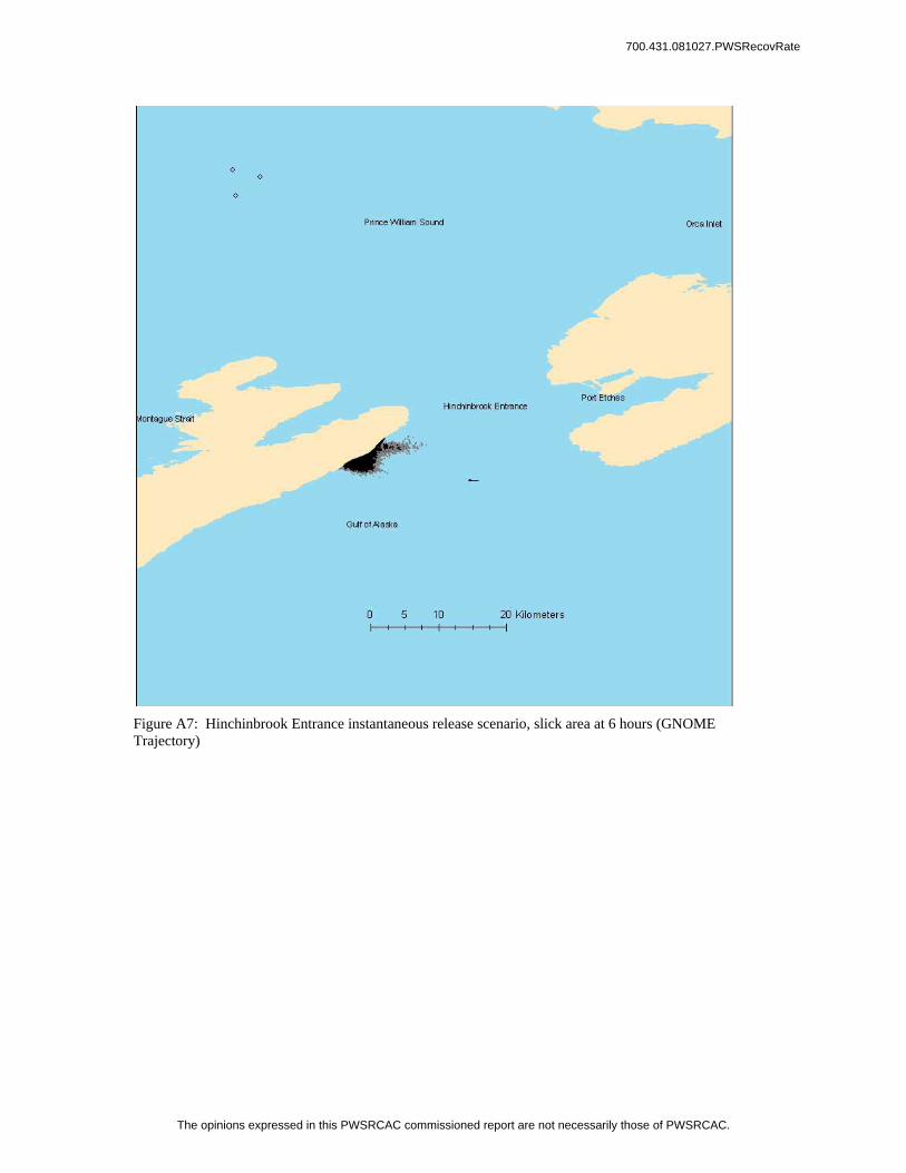
Figure A7: Hinchinbrook Entrance instantaneous release scenario, slick area at 6 hours (GNOME Trajectory)



Figure A8: Hinchinbrook Entrance instantaneous release, slick area at 72 hours (GNOME Trajectory)



A Comparison Between this Report and the 1993 ANVIL Study.1 1. PWSRCAC Question The ANVIL Study was used as the basis for the amount and type of equipment required to meet the 300,000 bbl response planning standard (RPS). Censum Northwest’s study predicts a shortfall of equipment and recommends different types and amounts of equipment to meet the RPS. To convince ADEC to modify the type and amount of equipment based on this new study, ADEC will need to understand the differences in the ANVIL Study vs. the Censum Northwest’s Response Rate Study, and will need to be convinced that the new study is more accurate and appropriate for predicting the type and amount of equipment required to meet the RPS. Censum Northwest should provide a comparison that explains the differences in assumptions and conclusions, and provide a compelling argument for PWSRCAC to advocate for additional equipment. “How does Censum Northwest’s assumptions and conclusions compare with the assumptions and recovery estimates found in the ANVIL study?” Censum Northwest Response In some important ways the Censum and ANVIL studies are similar in approach, assumptions, and conclusions. We first compare key assumptions and conclusions and subsequently provide a summary of differences. The greatest similarity between approaches is that both studies relied on mathematical calculations and theoretical tactics to derive their conclusions. Both studies calculate a theoretical capacity based on operational limitations. For example in the near-shore analysis both studies mathematically considered the capacity of each storage device and the need for off-loading prior to returning to service. Both studies considered fill cycle times and the number of fills possible per operational period. If encounter rate was not a limitation, both studies point to a theoretical possibility of recovering 300,000 barrels of oil in 72 hours.2 Finally both studies point out that the near shore recovery only accounts for a relatively small amount of the total recovered.

We believe the most fundamental difference between the two approaches is that only the Censum study attempts to describe a range of outcomes based on a variety of scenario factors and multiple calculations. The ANVIL study ignores some scenario factors and relies only on a single calculation. While the Censum study estimation could be refined through additional iterations using a broader array of scenario factors, we believe the range of outcomes developed provides a stronger understanding of actual capability, allows for the development of response plans in ways not previously considered, and does not set up unrealistic expectations.

1 The “Anvil Study” is a document titled HB 567 Compliance Submittal, October 29, 1993. 2 Our high-end calculation with a continuous release is 249,000 barrels. Theoretically it might be possible to achieve higher outcomes as high as 300,000 barrels, if for example, LEL concerns are neglected or in reality are not a concern. Skimming systems might then be deployed closer to the release location and achieve improve results.



Assumptions regarding encounter rate and emulsification account for the lion’s share of difference in the mathematical calculation outcomes between the two studies. Foremost is encounter rate. The Censum study considers encounter rate as a principal limitation, whereas, the Anvil Study does not. This assumption yields especially divergent calculation outcomes when considering instantaneous release scenarios.3 The ANVIL study lacks the sensitivity to account for the realistic expectation of changing encounter rates through time. The ANVIL study provides no scenario data illustrating an ever-expanding oil slick or an explanation why a set of spill trajectory scenarios was not considered. Section 4.7.2.1 of the ANVIL study suggests that most of the oil will be recovered from near the release site. This would only be possible if a continuous release were assumed, since an instantaneous release would drift away from the location of the vessel in a matter of hours. From Section 4.7.2.1:

“For large barges, each using two Transrec skimmers, are to be located closest to the damaged vessel. Therefore these barges would be recovering the freshest oil or emulsion.”

Also of note is the concept of “freshest” oil which only occurs when oil is continuously released. The ANVIL study does not provide any data regarding recovery system swath widths, which must be stated when considering encounter rate limitations. Differences in emulsification assumptions to a lesser extent affect differing calculation outcomes. Only for the near-shore response do the different sets of assumptions for emulsification play a significant role.4 The ANVIL study also does not consider evaporation, which plays an important role in reducing encounter rate, i.e., the less oil out there the less there is available to recover per unit area. The Censum study looked at two types of scenarios, instantaneous releases and continuous releases. This study’s instantaneous release scenario calculations illustrate what happens when encounter rate becomes an ever-increasing limitation. This study’s continuous release scenario calculations illustrate what happens when encounter rate and emulsification is less of a limiting factor. As discussed in the Censum study, if encounter rate were not a limiting factor then, at least mathematically, upwards towards 300,000 barrels of oil might be recovered during the initial 72 hours. We do not believe this is a realistic expectation and neither does the Anvil Study:

3 Censum study found that for an instantaneous release the resources available likely will not recover more than 23,000 barrels during the initial 72 hours. 4 For Open Water task forces we were instructed to assume no storage limitations. This assumption is justifiable given the ability to actively and successively separate and decant between storage chambers on the larger barges. We assumed no decanting for the near shore response because we believe decanting would prove to be inefficient in small barges, where there is less stability, and no opportunity to separate and decant between successive chambers prior to final discharge of oily water.



From the Introduction of the Anvil Study, p. i.

“Given the nature of a catastrophic spill, the Response Planning standards in HB 567 can not be expected to be met in actual performance. It is unrealistic to expect a 300,000-barrel oil spill could be cleaned up and that all needed equipment for a larger spill could be on scene and operating within a 72-hour period. Throughout the legislative and regulatory development of HB 567, the regulated community has repeatedly stressed that expectations in HB 567 were beyond the capability of technology and were without historical basis. For example, oil will elude containment and cleanup efforts; some oil will go ashore; weather, malfunctions and human performance will compromise efficiency, and all will contribute to an effectiveness that may be far less than that which can be illustrated in a theoretical, mathematical planning model.”

From Chapter 4.2, “Numerous variables relating to equipment performance, encounter rate, operational strategy and tactics, logistics, behavior of oil, weather and human factors would be difficult to duplicate in real-life. Moreover, this analysis relies on many specific assumptions, each having a varying degree of impact on the results. Therefore, while this analysis may be useful in that it provides some quantitative analysis of theoretical performance, it cannot be said to have examined or to provide conclusions about spill response capabilities that may exist in the actual response to a spill from a tanker.”



Summary of Assumptions and Affect on Recovery System Effectiveness ANVIL Study

Censum Study

Affect on Estimations

Slick dimensions and encounter rates not considered or loosely described.

Slick dimensions considered, swath width considered, encounter speed considered

A several fold decrease in expected performance occurs using the Censum study assumptions for instantaneous releases. The ANVIL study does not have the sensitivity to distinguish between instantaneous and continuous releases.

Recovery rate is equal to the ADEC recovery efficiency multiplied by the nameplate capacity.

ANVIL’s assumption is true only if the recovery rate does not exceed the encounter rate. Otherwise, assumed the same recovery efficiencies as the ANVIL study for the open-water response. Assumed only 5% efficiency for weir skimmers in the near-shore response.

As shown in the Censum study, when encounter rate is a limitation, there will be significantly decreased projected outcomes. A significant decrease in expected performance occurs for the near-shore response using the Censum study assumptions. However, this difference plays only a minor role in overall estimations, since the ANVIL study considers the near-shore capacity to be as less than 5% of the overall response capacity (Table 4-3 of ANVIL Study).

Emulsification expansion factor of 1.54

Emulsification expansion factor changes with time for instantaneous release over 72. Censum used the ADIOS II model to estimate the expansion factors. Expansion factors ranged from 1.0 at hour zero to 10 at hour 72.

Overall, a minor factor in total capacity estimations for both studies. A significant decrease in expected performance occurs for the near-shore response using the Censum study assumptions. However, this difference plays only a minor role in overall estimations, since the ANVIL study considers the near-shore capacity to be as less than 5% of the overall response capacity (Table 4-3 of ANVIL Study).

Evaporation not considered

Evaporation considered and incorporated as part of the thickness calculation.

A decrease in expected performance occurs using the Censum study assumptions, where evaporation could account for as much as 25% lost efficiency by hour 72.

Decanting factor of 0.8 for open-water and 0.4 for near-shore

Decanting factor of 100% for open-water and not allowed for near-shore

Overall, a significant factor, since not affecting on-water estimations. A decrease in expected performance for the near-shore response occurs using the Censum Study assumptions.

1.0 hour average transit time to unload recovered emulsion. Hook-up release of mini-barges takes 1 hour.

0.4 hour average transit time to unload recovered emulsion. Hook-up release of mini-barges takes 1 hour.

An increase in expected performance for near-shore response using Censum study assumptions. However, this plays only a minor role in overall capacity estimations.

Near-shore response does not include Current Busters but includes dracones.

Near-shore response includes Current Busters but excludes dracones.

The Censum study found that Current Buster task forces significantly improve the near-shore capacity, though that capacity is not as high as projected by the ANVIL analysis.



2. PWSRCAC Question: “Based on the findings of this report, how much more would the skimmers have to be de-rated to accurately reflect the lack of the skimmers to encounter the oil?” Currently, the skimmers are de-rated to 20% to account for a number of factors including operation in heavy weather, lack of continuous storage, debris, and etc. The skimmers should be de-rated even further considering the difficulty of encountering enough oil to skim. Censum Northwest Reply We believe de-rating poorly assesses response capacity and may adversely impact key response planning decisions. We do not suggest revising the de-rating, instead we suggest:

1) Strategically develop a set of representative scenarios, for example instantaneous releases and continuous releases.

2) Apply the ASTM standard to these scenarios. 3. PWSRCAC Question: “Could Censum Northwest look at the State of Alaska regulations and make a case for why encounter rates should be addressed as part of meeting the RPS?” Currently, State of Alaska regulations do not require an encounter rate analysis to fulfill the requirement for meeting the response planning standard. A case could be made that encounter rates should be part of that planning.” A Response Planning Standard or expectation to have the capability to recover 300,000 barrels of oil within 72 hours is a remarkable goal. Even with nearly perfect conditions it might not be possible to meet this goal with the existing response capacity. Under some scenarios it might be possible to approach this goal. For other scenarios this is simply not a realistic expectation. From the RCAC Response Gap Estimate we know that there are times when response will be impaired due to adverse winds and waves. The question to ask the State of Alaska is whether or not their expectation to have the ability to recover 300,000 barrels in 72 hours should be extended to include a broader array of scenarios than currently exists, yet still technologically feasible. The Censum study like the ANVIL study represents a mathematical analysis of recovery system effectiveness to illustrate what is theoretically possible. The Censum study includes a fundamental limitation not well addressed in the ANVIL study: Encounter Rates. Paying attention to this limitation may yield some startling results to those outside the response community. In good weather conditions it is unrealistic, even on paper, to expect to recover more than 50,000 barrels of oil in the first 72 hours, given a 300,000-barrel instantaneous release.



We believe the Censum analysis makes a strong case for why encounter rates should be considered when planning for oil spills. The most compelling reason is that better planning will yield better results for when a spill actually does occur. The Censum study found that encounter rate limitations, even in good weather could easily drive down expected outcomes by an order of magnitude (from over 200,000 barrels recovered to around 20,000 barrels recovered). We are not suggesting that it is reasonable to expect that 300,000 barrels be recovered from an instantaneous release; however, with additional planning efforts and some resource expenditures, improvements are possible, even in the face of a finite number of workboats and crew. As stated above, the key for improvement is to strategically define more scenarios of interest and then build the capacity to match these scenarios. The primary variable that should be adjusted from scenario to scenario is slick dimension.5 For some scenarios it may be determined that use of the large open-water recovery task forces does not maximize outcomes, given the number of workboats and crew available. Additional investment in high efficiency, high encounter speed recovery systems may improve results. Emphasis on larger numbers of portable storage devices may also improve results for some scenarios. Each of these types of scenarios can only be worked through if encounter rate limitations are fully considered.

5 Continuous releases with well defined plumes, convergences in high currents, large continuous slicks, large slicks that are broken up into patches, etc..



Bibliography Allen, A.A. 1991. “Controlled Burning of Crude Oil on Water Following the Grounding of the EXXON VALDEZ”. Proceedings, 1991 International Oil Spill Conference. American Petroleum Institute, Washington, D.C. Allen, A.A., and R.J. Ferek. 1993. Advantages and Disadvantages of Burning Spilled Oil. Proceedings, 1993 International Oil Spill Conference. American Petroleum Institute, Washington, D.C. ASTM Standards Volume 11.05, Section 11, 2007, “Water and Environmental Technology.” ASTM International, West Conshohocken, PA. www.astm.org. ASTM Standard F1780-97, 2007 (2002), “Standard Guide for Estimating Oil Spill Recovery System Effectiveness,” ASTM International, West Conshohocken, PA, www.astm.org. ASTM Standard F 625, “Practice for Classifying Water Bodies for Spill Control Systems,” ASTM International, West Conshohocken, PA, www.astm.org. ASTM Standard F 631, “Guide for Collecting Skimmer Performance Data in Controlled Environments,” ASTM International, West Conshohocken, PA, www.astm.org. ASTM Standard F 808, “Guide for Collecting skimmer Performance Data in Uncontrolled Environments,” ASTM International, West Conshohocken, PA, www.astm.org. ASTM Standard F 1523, “Guide for Selection of Booms in Accordance with Water Body Classifications,” ASTM International, West Conshohocken, PA, www.astm.org. Barnea, N., C.B. Henry, P. Roberts, and R.R. Laferriere. 1998. “Monitoring of In Situ Burning Operations.” Issue paper for the Minerals Management Service/National Institute of Standards and Technology Workshop on the In Situ Burning of Oil Spills, New Orleans, LA, November 1998.



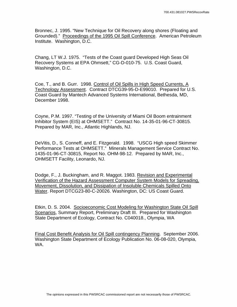
Bronnec, J. 1995. “New Technique for Oil Recovery along shores (Floating and Grounded).” Proceedings of the 1995 Oil Spill Conference. American Petroleum Institute. Washington, D.C. Chang, LT W.J. 1975. “Tests of the Coast guard Developed High Seas Oil Recovery Systems at EPA Ohmsett,” CG-D-010-75. U.S. Coast Guard, Washington, D.C. Coe, T., and B. Gurr. 1998. Control of Oil Spills in High Speed Currents, A Technology Assessment. Contract DTCG39-95-D-E99010. Prepared for U.S. Coast Guard by Mantech Advanced Systems International, Bethesda, MD, December 1998. Coyne, P.M. 1997. “Testing of the University of Miami Oil Boom entrainment Inhibitor System (EIS) at OHMSETT.” Contract No. 14-35-01-96-CT-30815. Prepared by MAR, Inc., Atlantic Highlands, NJ. DeVitis, D., S. Conneff, and E. Fitzgerald. 1998. “USCG High speed Skimmer Performance Tests at OHMSETT.” Minerals Management Service Contract No. 1435-01-96-CT-30815, Report No. OHM-98-12. Prepared by MAR, Inc., OHMSETT Facility, Leonardo, NJ. Dodge, F., J. Buckingham, and R. Maggot. 1983. Revision and Experimental Verification of the Hazard Assessment Computer System Models for Spreading, Movement, Dissolution, and Dissipation of Insoluble Chemicals Spilled Onto Water. Report DTCG23-80-C-20026. Washington, DC: US Coast Guard. Etkin, D. S. 2004. Socioeconomic Cost Modeling for Washington State Oil Spill Scenarios, Summary Report, Preliminary Draft III. Prepared for Washington State Department of Ecology, Contract No. C040018., Olympia, WA Final Cost Benefit Analysis for Oil Spill contingency Planning. September 2006. Washington State Department of Ecology Publication No. 06-08-020, Olympia, WA.



Goodwin, M.J., D.S. DeVitis, R.L. Cluster, D.L. Backer, S.L. Cunneff, and E.F. McClave. 1993. “OHMSETT Tests of NOFI Vee-Sweep 600 and NOFI 600S Oil Boom”. Report No. OHM-93-001, Minerals Management Service contract No. 14-35-0001-30544. Prepared by MAR, Inc., Rockville, MD. Goodwin, M.J., D.S. DeVitis, S.L. Cunneff, D.L. Backer, R.L. Cluster, and S. McHugh. 1994. “Ohmsett Tests of U.S. Coast Guard’s Vessel of Opportunity Skimming System.” Report No. OHM-94-02, Mineral Management Service contract No. 14-35-0001-30544. Prepared by MAR, Inc., Rockville, MD. “High Speed Skimmer Tests at Ohmsett.” 1996. Minerals Management Service contract 14-35-0001-30544. Prepared by MAR, Inc., Rockville, MD, November 1996. McClave, Edward F., David S. DeVitis, Susan Cummeff, James Nash, Roland Custer, Donald Backer, and Michael Goodwin. 1993. “Ohmsett Tests of RST Emergency Response Unit,” contract Report OHM-93-02. MAR, Inc. Edison, NJ. McClave, Edward F., David S. DeVitis, Susan Cummeff, James Nash, Roland Custer, and Scott McHugh. 1993. “Ohmsett Tests of Lori LSC-2 Skimming Systems,” Contract report OHM-94-01. MAR, Inc. Edison, New Jersey. McDonald, J.L. 1995. “The Morris J. Berman Spill: MSRC’s Offshore Operations.” Proceedings of the 1995 Oil Spill Conference. American Petroleum Institute. Washington, D.C. National Research Council (NRC). 1985. Oil in the Sea: Inputs, Fates, and Effects. National Academy Press, Washington, D.C. Nash, James H. 1984. “Testing of the Pick Up Polution (PUP) Oil collection Device.” Ohmsett contract No. 68-03-3056, Job Order 90. Environmental Protection Agency, Cincinnati. Oil Spill Response Vessel Capabilities in the State of Washington: Use of Commercial fishing and Other Vessels to Augment Oil Spill Response Capabilities. June 2005. Prepared for the State of Washington, Department of Ecology by The Glosten Associates, Contract No. C0500277, File No. 05051. Bellevue, WA.



Prince William sound Tanker Oil Discharge Prevention and Contingency Plan, June 2007. Schulze, R., ed. 1997. World Catalog of Oil spill Response Products, Sixth Edition. World Catalog JV, Annapolis, MD. U.S. Coast Guard, “Response Plan Equipment Caps Review,” COMDT CG-5431. http://www.uscg.mil/VRP/reg/capsreview.shtml. U.S. National Oceanic and Atmospheric Administration/Hazardous Materials Response and Assessment division (NOAA/HMRAD). 1994. ADIOS Automated Data Inquiry for Oil Spills. Version 1.1. Hazardous Materials and Response Assessment Division, U.S. National Oceanic and Atmoshoeric Adminsistrations, Seattle, WA. SERVS Technical Manual. 2007 Alyeska Pipeline Service Company, Valdez, Alaska.



prince william sound recovery rate analysis - … · prince william sound recovery rate analysis a...

Documents