Electronic copy of this paper is available at: http://ssrn.com/abstract=967363

“Pricing Prices”∗

Alex Boulatov†and Martin Dierker‡

C.T. Bauer College of Business, University of Houston, Houston, TX 77204

March 1, 2007

Abstract

Price quotes are a valuable commodity by themselves. This is a conundrum inthe standard asset pricing framework. We study the value of access to accurateand timely prices in a market economy explicitly taking into account that in theU.S., exchanges have property rights in the price quotes they generate. The factthat typically large institutions and sophisticated individuals obtain real time pricequotes motivates us to propose a simple model based on complementarity of privateinformation on the fundamentals and information on price. We find that grantingthe public access to real time pricing data has benefits such as stimulating the roleof stock market monitoring. Since the effect on liquidity can be negative, exchangesneed to be able to charge a fee for this service. In other situations, the exchangecan also benefit from free public disclosure of price quotes. We explicitly derive anequilibrium for differentially informed traders and a profit maximizing exchange.We confirm that, indeed, agents with the most precise private information willacquire real time price access. We outline several further empirical implications ofour model.

Keywords: Real-time prices; Sale of Information; Property rights; Market Efficiency;Liquidity

JEL classification: G.14; G.20

∗The authors would like to thank Hendrik Bessembinder who got us started thinking on the paper. We also benefittedgreatly from discussions with Paolo Fulghieri, Tom George, Praveen Kumar, Nisan Langberg, Natalia Piqueira, Craig Pirrongand seminar participants at the University of Houston. All remaining errors are our responsibility.

†Email: aboulatov@uh.edu. Phone (713) 743 4618.‡Email: mdierker@uh.edu. Phone (713) 743 4777.

Electronic copy of this paper is available at: http://ssrn.com/abstract=967363

1 Introduction

The prices of financial assets are a valuable commodity in and by themselves. Sales of trans-

action data produced revenue of $167 million for the NYSE alone in 20041. In the standard

asset pricing theory (Huang-Litzenberger 1988, Cochrane 2005), this is a conundrum. On

the other hand, Roll (1984) has shown that enough useful information is contained in market

prices to predict the weather in Florida orange groves. Thus, access to accurate, transparent,

and timely market prices has great value to both dealers (like orange juice futures traders)

and producers (like orange growers who can undertake protective measures against a freeze).

The value of the information contained in prices can best be measured by agent’s willingness

to pay for it (Grossman and Stiglitz 1980). We thus analyze the “price of prices” as an

important characteristic of the financial market.

The fact that agents are willing to pay hundreds of thousands of dollars per year to obtain

real time price access via Reuters or Bloomberg cannot easily be addressed within the stan-

dard asset pricing framework, where agents are typically modelled by preferences they have

over lotteries, and financial markets are viewed as elaborate and complex, but nevertheless

gambles. Nobody would pay for data on past or current outcomes of a (manipulation-free)

gamble. We conclude that financial markets are more than a lottery, and that they produce

high-quality market prices as a valuable output.

To study this issue, we explicitly take into account the U.S., financial exchanges have

property rights in the price quotes they generate2 (Mulherin et al., 1991). This was decided

in a landmark 1905 Supreme Court verdict3, in which “the court stated that it was unlikely

the market for future sales was merely gambling since the prices are so important in business

and farming.”4 We develop a model of strategic trading in the spirit of Kyle (1985). In our

model, agents have access to information about the value of an asset. But since agents do

not know the most recent price of the asset, they face a source of execution risk when trading

in the markets. For instance, if an agent knows that the stock is worth $100, but does not

know whether it is currently trading at $98 or $102, then the value of his information is

1According to the NYSE’s financial statements. We expect similar magnitude of revenues for other exchanges such as theCBOT.

2This includes property rights in data derived from the exchange’s price quotes. Certain limitations apply, as discussedbelow.

3Board of Trade of the City of Chicago v. Christie Grain and Stock Company, 198 U.S. 236 (1905)4Quote taken from Mulherin et al. (1991)

1

greatly diminished. We solve for the unique linear equilibrium in an economy in which the

exchange has property rights in market prices. Since prices are semi-strong efficient in the

model, agents do not get an informational advantage over the market maker by purchasing

real-time price access. The“price of prices” is positive only because real-time pricing data is

a complement to the private information agents possess.

Our paper is closely related to the literature on the sale of information (Admati and

Pfleiderer (1986, 1990)). In both cases, agents benefit from an improved forecast of asset

mispricing E(Vt − Pt). While the existing literature has focused on the acquisition of infor-

mation on the fundamental value Vt, we find that agents can also improve their forecast of

the anticipated price differential by observing Pt more precisely, which explains why they

are willing to pay for a subscription to real-time price information. Note that the seller’s

incentives are different, since the exchange’s primary business is facilitation of trade, not

data sales. We explicitly consider this in our analysis. In the existing literature, indirect sale

of information (e.g., via a mutual fund) is typically optimal (Admati and Pfleiderer (1990)).

Instead, we find that exchanges sell real time price data directly. This is because (i) real

time price data is only valuable in conjunction with private information, and thus indirect

sale of information leads to zero revenue and (ii) truthful sale of pricing information by the

exchange is incentive compatible, since the data is ex-post verifiable.

In the presence of a single informed trader, access to real time prices is valuable, but

comes at the expense of lower market liquidity. This prevents the exchange from publicly

disclosing its price quotes even though access to real time pricing information improves the

effectiveness of financial markets as monitors (Holmstrom and Tirole, 1993). Indeed, we find

that the exchange is indifferent between selling information or not. This is no longer the

case when we introduce endogenous information acquisition. We find that sale of real time

pricing information is beneficial because it eliminates the need to produce information that

is already incorporated into prices. Furthermore, it increases the marginal utility of private

information, which in turn increases the usefulness of market prices to monitor management.

When multiple informed agents compete in financial markets, they may find it in their

interest to acquire real time pricing information even if, as a group, informed traders would

benefit from abstaining to do so. Indeed, we show that the exchange maximizes its profits

(and, simultaneously, market efficiency) by selling real time information to all informed

2

agents5). Specifically, we show that the exchange always sells a signal on price information

to all (or at least many) informed traders. Consistent with the availability of real time

data, this signal is of high or infinite precision. Furthermore, we show conditions under

which the exchange benefits from the public availability of a second signal of (considerably)

lower precision. The exchange can benefit from the free disclosure of price information in

two ways. Firstly, such a disclosure can level the playing field and thus improve market

liquidity. Secondly, providing informed traders with more information can intensify the

degree of competition among them, which in turn increases their willingness to pay for the

high precision signal.

When informed agents differ along the precision of their respective private signals, we

show that it is the agents with the most precise private information who have the highest

marginal utility of accurate pricing information. At the same time, we prove that selling real

time data to these agents has detrimental effects on market liquidity. The resulting tension

leads to a challenging but interesting profit maximization problem for the exchange. The

equilibrium ”price of prices” can be characterized as a cost schedule when the cost increases

in the precision of the current price signal. We show conditions under which an equilibrium

exists and show that better informed agents indeed purchase more precise real time price

data. This confirms the empirical fact that it is well informed, highly specialized traders

who pay substantial amounts of money to obtain access to real time pricing data.

The ”price of prices” that agents pay varies. Individual investors can receive real-time

pricing data from a source such as Yahoo.com for a nominal fee (as of Dec. 2006, this

fee is $13.95 per month)6, or they receive it for free from their broker (and indirectly pay

by trading with the broker). For institutional investors who subscribe to professional data

service through a company such as Reuters, they need to directly pay the exchange. In case

of the NYSE, the fee is $5,000 per month plus a $60 fee for every display unit (as of Dec.

2006)). The latter fee is lowered by $10 if the recipient can is willing to accept a five second

delay.

We focus primarily on the timeliness of price quotes as one dimension of the economic value

of prices. In addition, accurate pricing information is needed to implement advanced trading

5In contrast to Admati and Pfleiderer (1986, 1990), where sale to a subset of potentially informed agents is optimal. Ourresult is due to the exchange taking the impact of data sales on liquidity into account.

6As of January 2007, the NYSE is asking the SEC for permission to sell real time data to websites at $100,000 a month.

3

strategies or detecting small arbitrage opportunities. Academic researchers are probably

familiar with the “price of prices” from their own experience in acquiring costly data sets.

Besides the dimensions previously mentioned, reliability and comprehensiveness determine

the value of pricing data. Only large data sets without errors can lead to a maximum of

information content being extracted from the data. It is thus not surprising that Wall Street

firms invest in the maintenance and protection their own data-sets, as they are useful in

their trading activities.

How to arrange the trading process in the most efficient way has been a central question

in the microstructure literature. For this purpose, researchers have introduced a number of

measures of market liquidity and informational efficiency. No single sufficient statistic for

the quality of a market can be developed. We add the “price of prices” to the list of existing

variables as a direct measure of the usefulness of information contained in market prices. The

fact that the major exchanges receive a substantial portion of their total revenue from data

sales indicates that, despite recent debates on market irrationality, the information content

of stock prices is considerable.

In our paper, we establish the economic value of access to accurate and timely market

prices. At the same time, it is striking that real time prices are so valuable, given that

briefly delayed quotes are free. While we provide conditions under which the exchange

benefits from the free disclosure of a noisy public signal, we view the question of an optimal

delay time (typically 10 to 30 minutes, as seen in Table 1) as essentially an empirical one7.

We believe that the value of pricing access for speculative trading is greatly diminished after

a 15 minutes delay. Early studies such as such as Patell and Wolfson (1984), Jennings and

Starks (1985), and Barclay and Litzenberger (1988) examine the speed of price response to

various corporate announcements such as dividends, earnings, and equity offerings. They

find that prices incorporate news within five to fifteen minutes, which perfectly corresponds

to a high economic value of real-time prices, while a 15 minute delay will preclude significant

trading profits. Kim et al. (1997) report a similar time frame for the reaction to analyst buy

recommendations. Busse and Green (2002) provide some evidence that markets react to TV

stock buy recommendations much quicker, often within seconds up to a minute. However,

7In what follows, we view the occurrence of a public news event as the origin of private information for informed agents, asin Kandel and Pearson (1995). We find it essential to explain the price of prices in a market that is efficient in the semi strongsense.

4

the response to sell recommendations is more gradual, “lasting fifteen minutes, perhaps due

to the higher costs of short-selling.” We conclude that a high price of real time quotes and

a low price of quotes with a fifteen minute delay is consistent with the empirically observed

speed of market reaction to news events.

This implies that private information on the fundamentals and pricing information are

complementary. We propose a simple model based on information complementarity explain-

ing the stylized facts described above. We explicitly derive an equilibrium for differentially

informed traders. We show that in order to extract maximum profits, the exchange should

sell price information according to a certain cost schedule with higher cost for higher preci-

sion. Our model has several further empirical implications.

This by no means implies that delayed price quotes are worthless. Indeed, they can be

viewed as a public good, helping for instance in the valuation of large portfolio positions. A

portfolio of liquidly traded securities in markets with good price discovery is much easier to

value than, for instance, a portfolio of energy derivatives such as ENRON had8. Similarly,

an agent engaging in optimal portfolio choice still values accurate price quotes with a short

delay, as they will help him allocate funds more efficiently. In fact, the legal system has

placed limitations unto the exchange’s property rights in price quotes that align with this

view. For instance, agents are allowed to use an exchange’s settlement price as the basis for

the creation of derivatives products9.

This paper is structured as follows. We present our model in section 2. We solve for

equilibrium and analyze its implications for the price of prices in section 3. We examine far

more complex information allocations in section 4 and provide implications and conclusions

of our analysis in section 5.

2 The Model

We consider a model of price formation in securities markets with strategic traders along the

lines of Kyle (1985). However, we modify the model to explicitly incorporate the institutional

fact that exchanges have the property rights to the prices they generate (Mulherin et al.

8The absence of transparent market prices have led people to doubt the valuations ENRONattributed to their portfolio.

9The New York Mercantile Exchange (NYMEX) filed and lost a lawsuit against the Inter-continental Exchange (ICE), trying to prohibit ICE from doing exactly that.

5

1991). Specifically, we assume that a single risky asset is traded at times t = 1, . . . , T . In

each time period t, the asset generates a random cash flow of δt, which we assume to be

Normally distributed with mean zero and variance σ2δ . Similar to Admati and Pfleiderer

(1988), the asset does not pay dividends, resulting in a “liquidation” value of the asset at

the beginning of period t of

Vt =t−1∑s=1

δs. (1)

We assume that all δt’s are jointly independent. The risk-free rate in this economy is nor-

malized to zero.

We assume three types of risk-neutral agents in our model: Uninformed (liquidity) traders,

informed traders, and competitive market makers. We assume that in each period t, a group

of short-lived informed and liquidity traders are born just before markets open. They trade

once when markets open at time t and realize their profits or losses. They then consume

and leave the economy to make room for a new generation of traders.

The generation of noise traders collectively submit a demand of ut ∼ N(0, σ2u) at time

t. In addition, there is a generation of nt agents that have access to information about the

asset’s cash flow δt prior to trading. Specifically, we assume that agent k receives a signal

Sk,t = Vt+1 + εk,t (2)

about the value of the asset. The error terms εk,t are Normally distributed with mean zero

and variance σ2ε,k. We assume that the cross-sectional correlation of the error terms is zero.

Based on their private information, agents may choose to submit buy or sell orders to an

exchange, where the asset is traded.

Following Kyle (1985), we assume that prices are set by risk-neutral, competitive market

makers working at the exchange, who observe the aggregate net order flow. As in and Admati

and Pfleiderer (1988), the market makers observe the cash flow δt at the end of each trading

round and set the market efficient price. We assume that the asset value at the end of period

t, Vt, becomes publicly and costlessly available after m periods of trade. This assumption

parallels the institutional feature that price quotes generally become public after a period of

15 or 20 minutes.

Thus, informed agents who want to trade on their private information face an execution

risk. While they know the fundamental value of the company, they face uncertainty about

6

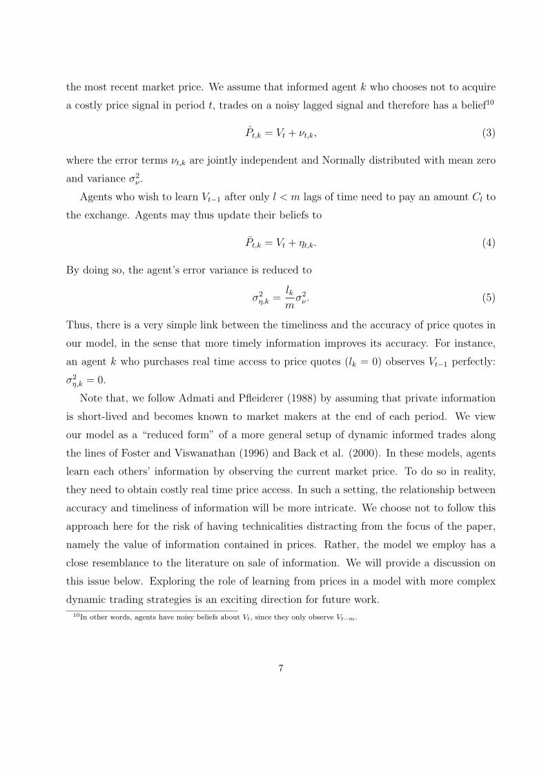
the most recent market price. We assume that informed agent k who chooses not to acquire

a costly price signal in period t, trades on a noisy lagged signal and therefore has a belief10

Pt,k = Vt + νt,k, (3)

where the error terms νt,k are jointly independent and Normally distributed with mean zero

and variance σ2ν .

Agents who wish to learn Vt−1 after only l < m lags of time need to pay an amount Cl to

the exchange. Agents may thus update their beliefs to

Pt,k = Vt + ηt,k. (4)

By doing so, the agent’s error variance is reduced to

σ2η,k =

lkm

σ2ν . (5)

Thus, there is a very simple link between the timeliness and the accuracy of price quotes in

our model, in the sense that more timely information improves its accuracy. For instance,

an agent k who purchases real time access to price quotes (lk = 0) observes Vt−1 perfectly:

σ2η,k = 0.

Note that, we follow Admati and Pfleiderer (1988) by assuming that private information

is short-lived and becomes known to market makers at the end of each period. We view

our model as a “reduced form” of a more general setup of dynamic informed trades along

the lines of Foster and Viswanathan (1996) and Back et al. (2000). In these models, agents

learn each others’ information by observing the current market price. To do so in reality,

they need to obtain costly real time price access. In such a setting, the relationship between

accuracy and timeliness of information will be more intricate. We choose not to follow this

approach here for the risk of having technicalities distracting from the focus of the paper,

namely the value of information contained in prices. Rather, the model we employ has a

close resemblance to the literature on sale of information. We will provide a discussion on

this issue below. Exploring the role of learning from prices in a model with more complex

dynamic trading strategies is an exciting direction for future work.

10In other words, agents have noisy beliefs about Vt, since they only observe Vt−m.

7

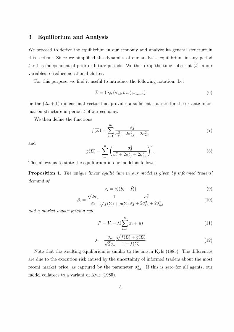
3 Equilibrium and Analysis

We proceed to derive the equilibrium in our economy and analyze its general structure in

this section. Since we simplified the dynamics of our analysis, equilibrium in any period

t > 1 is independent of prior or future periods. We thus drop the time subscript (t) in our

variables to reduce notational clutter.

For this purpose, we find it useful to introduce the following notation. Let

Σ = (σδ, (σε,i, ση,i)i=1,...,n) (6)

be the (2n + 1)-dimensional vector that provides a sufficient statistic for the ex-ante infor-

mation structure in period t of our economy.

We then define the functions

f(Σ) =nt∑i=1

σ2δ

σ2δ + 2σ2

ε,i + 2σ2η,i

(7)

and

g(Σ) =n∑

i=1

(σ2

δ

σ2δ + 2σ2

ε,i + 2σ2η,i

)2

. (8)

This allows us to state the equilibrium in our model as follows.

Proposition 1. The unique linear equilibrium in our model is given by informed traders’

demand of

xi = βi(Si − Pi) (9)

βi =

√2σu

σδ

1√f(Σ) + g(Σ)

σ2δ

σ2δ + 2σ2

ε,i + 2σ2η,i

(10)

and a market maker pricing rule

P = V + λ(n∑

i=1

xi + u) (11)

λ =σδ√2σu

√f(Σ) + g(Σ)

1 + f(Σ)(12)

Note that the resulting equilibrium is similar to the one in Kyle (1985). The differences

are due to the execution risk caused by the uncertainty of informed traders about the most

recent market price, as captured by the parameter σ2η,i. If this is zero for all agents, our

model collapses to a variant of Kyle (1985).

8

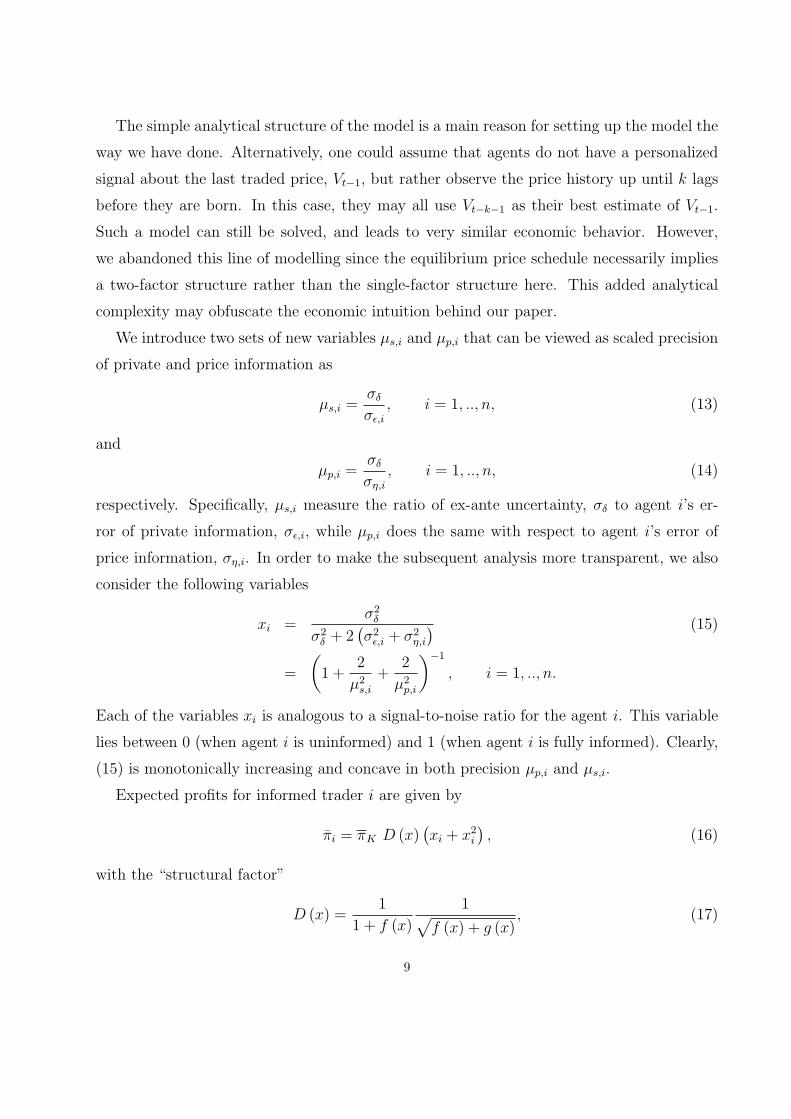
The simple analytical structure of the model is a main reason for setting up the model the

way we have done. Alternatively, one could assume that agents do not have a personalized

signal about the last traded price, Vt−1, but rather observe the price history up until k lags

before they are born. In this case, they may all use Vt−k−1 as their best estimate of Vt−1.

Such a model can still be solved, and leads to very similar economic behavior. However,

we abandoned this line of modelling since the equilibrium price schedule necessarily implies

a two-factor structure rather than the single-factor structure here. This added analytical

complexity may obfuscate the economic intuition behind our paper.

We introduce two sets of new variables µs,i and µp,i that can be viewed as scaled precision

of private and price information as

µs,i =σδ

σε,i

, i = 1, .., n, (13)

and

µp,i =σδ

ση,i

, i = 1, .., n, (14)

respectively. Specifically, µs,i measure the ratio of ex-ante uncertainty, σδ to agent i’s er-

ror of private information, σε,i, while µp,i does the same with respect to agent i’s error of

price information, ση,i. In order to make the subsequent analysis more transparent, we also

consider the following variables

xi =σ2

δ

σ2δ + 2

(σ2

ε,i + σ2η,i

) (15)

=

(1 +

2

µ2s,i

+2

µ2p,i

)−1

, i = 1, .., n.

Each of the variables xi is analogous to a signal-to-noise ratio for the agent i. This variable

lies between 0 (when agent i is uninformed) and 1 (when agent i is fully informed). Clearly,

(15) is monotonically increasing and concave in both precision µp,i and µs,i.

Expected profits for informed trader i are given by

πi = πK D (x)(xi + x2

i

), (16)

with the “structural factor”

D (x) =1

1 + f (x)

1√f (x) + g (x)

, (17)

9

where

f (x) =n∑

j=1

xj, g (x) =n∑

j=1

x2j , (18)

and are scaled by the expected insiders’ payoff in Kyle (1985) model

πK =1

2σδσu. (19)

Importantly, the structural factor D (x) depends on the entire information distribution across

the informed agents, while each of the the parameters xi, i = 1, ..n characterizes the

information set of a particular agent. The inverse market liquidity takes the form

λ (x) = λK

√2√

f (x) + g (x)

1 + f (x), (20)

with the standard inverse market depth parameter (Kyle 1985)

λK =σδ

2σu

. (21)

There is a close resemblance to the well-established literature on the sale of information

(see, among others, Admati and Pfleiderer 1986, 1990). This can best be seen when we

examine the individual agent’s trading strategy xi = βi(Si− Pi). As in the literature on the

sale of information, the trading strategy is linear in the anticipated price differential. From a

modeling perspective, the difference is that the existing literature has focused on improving

the agent’s forecast of next period price (denoted Si in our model). In this paper, however,

we argue that the agent will not perfectly observe current price (denoted Pi). Rather, the

agent needs to purchase real time price data to improve his estimate about anticipated price

appreciation of the asset. This similarity to the existing literature explains why some of the

special cases we examine in section 3 bear a certain resemblance to existing results. At the

same time, this enables us to adopt the intuition from existing models and apply it to our

analysis.

Following this intuition, we can identify several dimensions along which we differ from

the existing literature. Firstly, we consider the sale of data, not information. Since the data

is ex-post verifiable, we can easily overcome concerns about the seller’s incentives to sell

information truthfully. “Lying” by the exchange is not a concern.

Indeed, the seller of information is an entirely different entity. In fact, it is not the ex-

change’s primary business to sell data. Rather, the exchange needs to facilitate smooth

10

trading to maximize listing fees and attract buyers and sellers. In what follows, we will

specifically analyze how the sale of data impacts the behavior of the exchange and param-

eters of the trading system. It may even be the case that the exchange benefits from a

free disclosure of real-time price data - something that could never happen in the existing

literature on the sale of information.

Last but not least, the value of the information contained in real-time prices is probably

highly limited for individual and passive investors. It is probably well-informed private

individuals and institutions who benefit the most of real-time data access11. We capture this

spirit in our model, where real-time price access is only valuable in conjunction with private

information. This is in contrast to the literature on the sale of information, in which anyone

can gain a valuable advantage from purchasing information.

Our paper differs from the existing literature on the sale of information in the following

sense. In Admati and Pfleiderer (1986, 1990), it is often optimal to sell information indirectly

(i.e., by setting up a mutual fund), as this (i) mitigates truth-telling constraints and (ii) often

leads to higher revenue due to avoidance of competition among informed traders. In the case

of exchanges selling real-time transaction data, this is typically done directly, since (i) the

data is ex-post verifiable and (ii) individual agents need to combine real time pricing data

with their own private information to reap trading profits. In the setting of our model,

indirect sale of information would generate zero revenue, since the exchange does not have

any private information it can combine with real time pricing data (by definition, the stock

price already reflects all the exchange’s information).

3.1 Analysis

We now proceed to analyze the equilibrium we derived above. Specifically, we investigate

the exchange’s decision to potentially sell pricing data, and the informed agents’ incentives

to acquire them. It is important to recognize that the sale of price and transactions data is

not the prime business of an exchange. Certainly, the exchange cannot maximize revenue

from data sales without taking the impact of such a sale on price discovery and market

liquidity into account. Thus, as in Holmstrom and Tirole (1993), we assume that firms need

11Presumably, the information contained in real-time prices is also valuable to financial intermediaries, institutions whoexecute massive trades, and liquidity providers who may act as market makers. We abstract from these issues for the sake ofsimplicity.

11

to compensate all or at least some of uninformed traders for their expected losses to better

informed market participants. Specifically, let q ∈ [0, 1] denote the fraction of uninformed

trader’s losses the exchange needs to reimburse (we can think of q as the exchange’s shadow

price of liquidity). We assume that the firm is willing to offer the exchange a (constant) listing

fee Q, from which the firm subtracts the expected compensation of uninformed traders, which

are given by qλσ2u. In addition, the exchange can earn additional revenue by selling its pricing

data to informed traders. Let C(i) ≥ 0 denote the dollar amount that informed agent i is

willing to spend on acquiring pricing data (given the exchanges pricing scheme (c1, . . . , cm)).

The exchange’s problem is now to

maxc1,...,cm

Q− qλσ2u +

n∑i=1

C(i) (22)

Alternatively, this maximization problem can be rationalized by the idea that exchanges

compete for order flow, as in Huddart, Hughes, and Brunnermeier (1999). Thus, the effect

of the exchange’s sale of information on market liquidity directly affects the exchange’s profit.

The intuition is as follows. If sale of information reduces market depth, then the exchange

has to compensate uninformed traders for higher trading costs to attract their orders (and

vice versa). The parameter q will be dictated by the degree of competition, where q = 1

represents perfect competition among exchanges.

To guide our economic intuition, we conduct our analysis in three steps. First, we analyze

the case of a monopolistic informed trader. Second, we allow any positive number of informed

traders, nt, with the same precision of their information. In the third and final step, we

analyze the general case of multiple agents with different information quality. For the sake

of economic intuition, we will start with the case of m = 1, i.e. the exchange either selling

a signal of perfect precision, or no information12. We then proceed to investigate which

agents purchase more informative signals if the exchange offers a menu of different signals

at different prices. Furthermore, we focus on perfect competition among exchanges initially

(q = 1), and revisit the more general case subsequently.

12We eliminate the first trading period, t = 1, from our consideration here, since there is nouncertainty about past transaction prices. Period 1 is identical with a standard Kyle model.

12

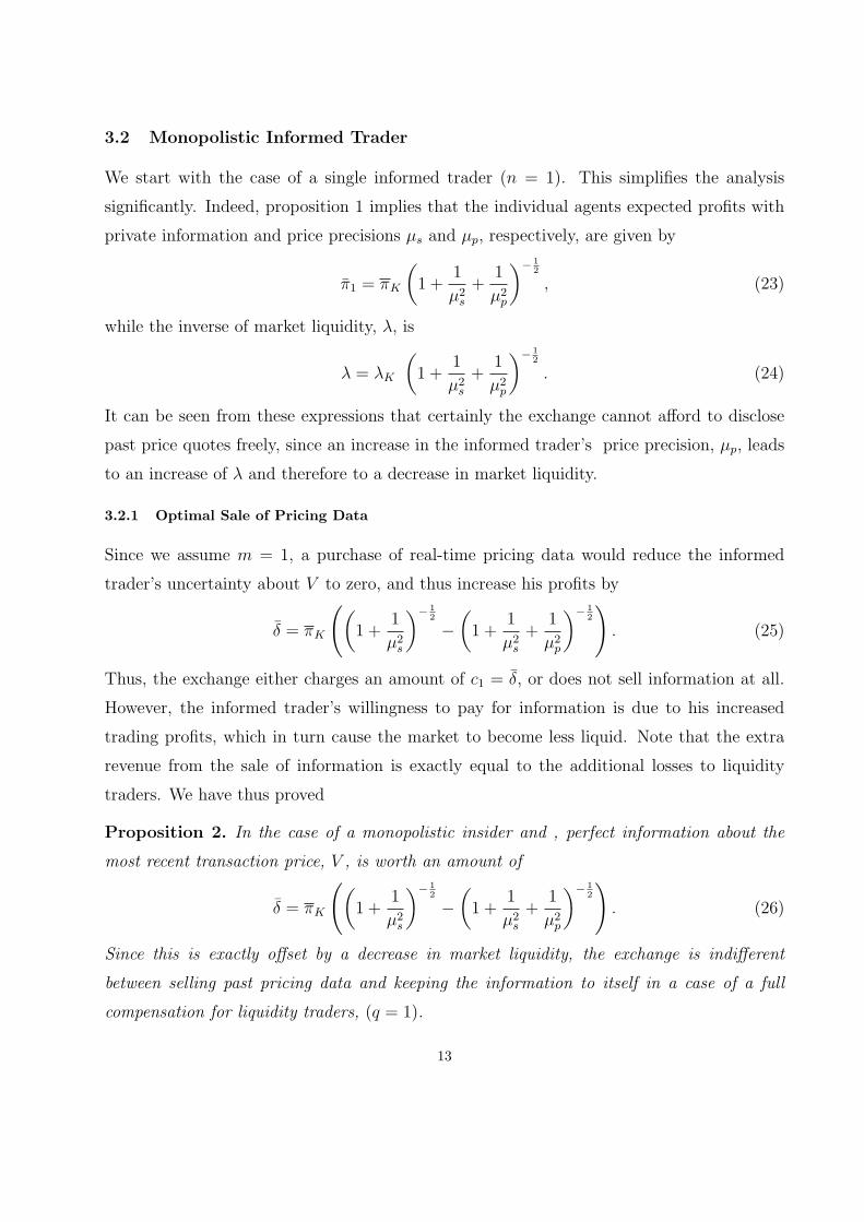
3.2 Monopolistic Informed Trader

We start with the case of a single informed trader (n = 1). This simplifies the analysis

significantly. Indeed, proposition 1 implies that the individual agents expected profits with

private information and price precisions µs and µp, respectively, are given by

π1 = πK

(1 +

1

µ2s

+1

µ2p

)− 12

, (23)

while the inverse of market liquidity, λ, is

λ = λK

(1 +

1

µ2s

+1

µ2p

)− 12

. (24)

It can be seen from these expressions that certainly the exchange cannot afford to disclose

past price quotes freely, since an increase in the informed trader’s price precision, µp, leads

to an increase of λ and therefore to a decrease in market liquidity.

3.2.1 Optimal Sale of Pricing Data

Since we assume m = 1, a purchase of real-time pricing data would reduce the informed

trader’s uncertainty about V to zero, and thus increase his profits by

δ = πK

((1 +

1

µ2s

)− 12

−(

1 +1

µ2s

+1

µ2p

)− 12

). (25)

Thus, the exchange either charges an amount of c1 = δ, or does not sell information at all.

However, the informed trader’s willingness to pay for information is due to his increased

trading profits, which in turn cause the market to become less liquid. Note that the extra

revenue from the sale of information is exactly equal to the additional losses to liquidity

traders. We have thus proved

Proposition 2. In the case of a monopolistic insider and , perfect information about the

most recent transaction price, V , is worth an amount of

δ = πK

((1 +

1

µ2s

)− 12

−(

1 +1

µ2s

+1

µ2p

)− 12

). (26)

Since this is exactly offset by a decrease in market liquidity, the exchange is indifferent

between selling past pricing data and keeping the information to itself in a case of a full

compensation for liquidity traders, (q = 1).

13

This proposition differs from results of Admati and Pfleiderer (1986), since the exchange

needs to compensate the expected losses of liquidity traders. While the proposition estab-

lishes the value of pricing information, but questions remain. What are the welfare effects

of the exchange selling pricing information? Are there situations in which the exchange can

generate positive profits from the sale of data? We will proceed to answer these questions

in turn.

First, we note that the informational efficiency of the stock market increases when the

exchange supplies costly transaction data. The uncertainty about the asset’s fundamental

value that is not revealed in market prices, V ar(V +δ|P ), is found to decrease by an amount

ofσ2

δ

2

((1 +

1

µ2s

)−1

−(

1 +1

µ2s

+1

µ2p

)−1)≥ 0. (27)

Therefore, while the exchange is indifferent between selling pricing data or not doing so in

a case of a full compensation (q = 1), society clearly prefers the additional welfare benefits

of having more efficient markets. These benefits can originate from a mitigation of agency

conflicts and improved executive compensation (Holmstrom and Tirole 1993) or from more

efficient investment decisions (Fishman and Haggerty 1989). But the sale of pricing data has

additional welfare implications that become clear once we allow for endogenous information

acquisition.

3.2.2 Endogenous Information Production

We now investigate a situation in which the informed trader is not endowed ex-ante with

information, but needs to engage in costly research to uncover it (Holmstrom and Tirole

1993, Verrecchia 1982). Specifically, we assume that, at a cost of cε(x), the agent can obtain

a signal about the final payoff of the firm with precision x (the only change to the previous

model is that the error variance σ2ε, = 1/x is now endogenous). Similarly, let cη(y) denote

the cost the agent needs to incur to obtain a signal about the most recent transaction price,

V , with precision y = 1/σ2η,1. We follow the literature in assuming that the cost functions cε

and cη are monotonically increasing, convex and differentiable.

In the absence of the exchange selling a signal to the informed, these assumptions assure

that there exists a unique equilibrium at the information acquisition stage. In equilibrium,

14

the informed investor acquires a positive signal precision about both the liquidation value of

the asset and the most recent transaction price. Let (σ2ε,1, σ

2η,1) denote the agent’s optimally

chosen error variances.

We proceed to obtain some economic insights into the effects of allowing the (possibly

costly) disclosure of transaction price data. Firstly, such a disclosure eliminates the need for

the informed trader to engage in costly research about the current market price. This repre-

sents an immediate welfare gain of cη(1/σ2η,1), since spending resources to obtain information

that society already possesses is redundant.

Furthermore, disclosing real time pricing data stimulates private information production,

thus leading to improved market efficiency and stock market monitoring. Specifically, if they

acquire real time pricing data, their error variance becomes ση,1 = 0 < σ2η,1. This in turn

increases the marginal utility of private information, and thus induces the informed agent

to acquire more precise signal about the asset’s fundamental value. Let 1/σ2ε,1 denote the

agent’s optimally chosen precision of private information. It follows that σ2ε,1 ≤ σ2

ε,1. This

will result in improved informational efficiency of the market.

We have thus established the welfare gains from disclosure of current transaction prices.

However, since such a disclosure leads to more informed trade, market liquidity will deterio-

rate. Thus, the exchange cannot simply disclose this information freely, but needs to sell it.

We summarize our results in the subsequent proposition.

Proposition 3. A (potentially costly) disclosure of real-time pricing data increases the effec-

tiveness of stock market monitoring by leading to more private information production. An

additional welfare gain accrues since the informed agent does not need to produce information

about current prices that is already known to the market.

Again, since there is a monopolistic informed trader, the increase in market monitoring

activity comes at the expense of larger losses to uninformed shareholders. The exchange

thus needs to charge the informed trader for access to real time prices. Whether it will

be profitable for the exchange to sell pricing data or not depends on the relative costs of

producing private information about asset value versus information about current market

price. The issue of a profitable sale of pricing information will become much more clear when

we introduce competition among multiple informed traders below.

15

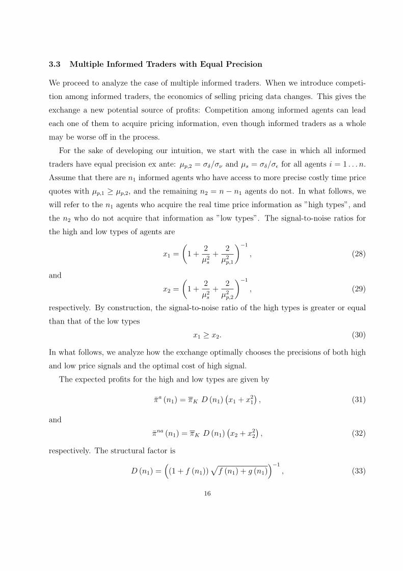
3.3 Multiple Informed Traders with Equal Precision

We proceed to analyze the case of multiple informed traders. When we introduce competi-

tion among informed traders, the economics of selling pricing data changes. This gives the

exchange a new potential source of profits: Competition among informed agents can lead

each one of them to acquire pricing information, even though informed traders as a whole

may be worse off in the process.

For the sake of developing our intuition, we start with the case in which all informed

traders have equal precision ex ante: µp,2 = σδ/σν and µs = σδ/σε for all agents i = 1 . . . n.

Assume that there are n1 informed agents who have access to more precise costly time price

quotes with µp,1 ≥ µp,2, and the remaining n2 = n − n1 agents do not. In what follows, we

will refer to the n1 agents who acquire the real time price information as ”high types”, and

the n2 who do not acquire that information as ”low types”. The signal-to-noise ratios for

the high and low types of agents are

x1 =

(1 +

2

µ2s

+2

µ2p,1

)−1

, (28)

and

x2 =

(1 +

2

µ2s

+2

µ2p,2

)−1

, (29)

respectively. By construction, the signal-to-noise ratio of the high types is greater or equal

than that of the low types

x1 ≥ x2. (30)

In what follows, we analyze how the exchange optimally chooses the precisions of both high

and low price signals and the optimal cost of high signal.

The expected profits for the high and low types are given by

πa (n1) = πK D (n1)(x1 + x2

1

), (31)

and

πna (n1) = πK D (n1)(x2 + x2

2

), (32)

respectively. The structural factor is

D (n1) =((1 + f (n1))

√f (n1) + g (n1)

)−1

, (33)

16

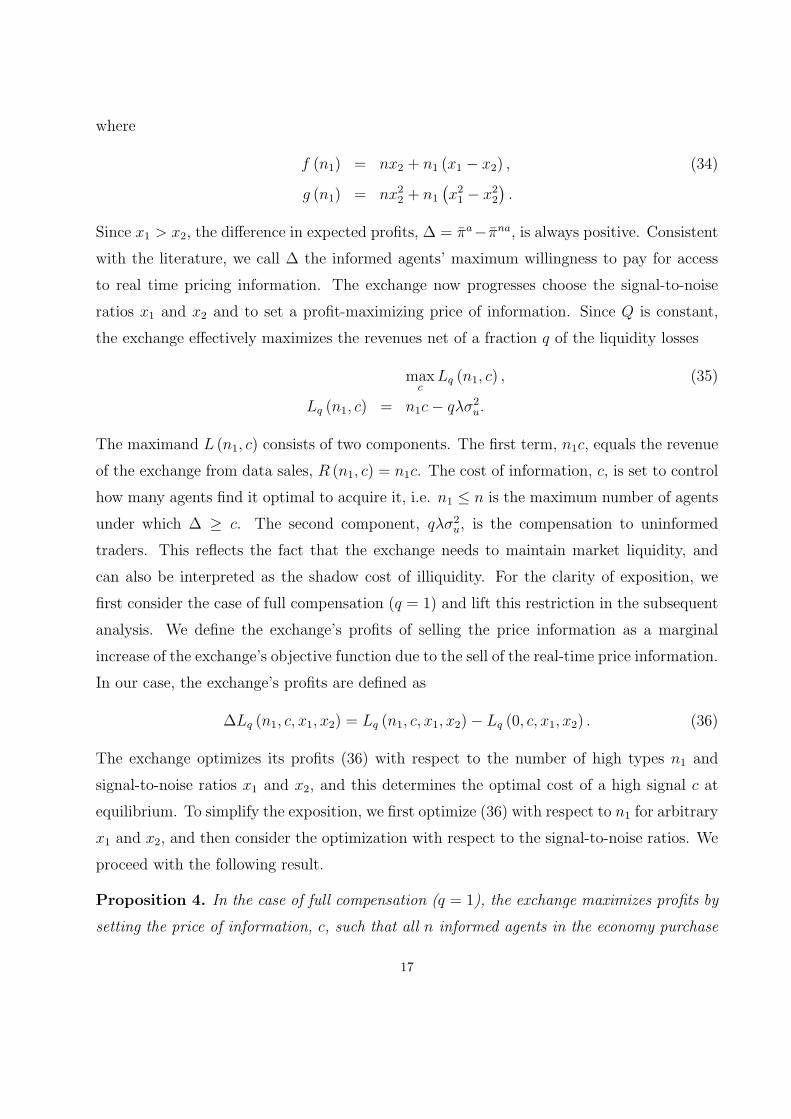
where

f (n1) = nx2 + n1 (x1 − x2) , (34)

g (n1) = nx22 + n1

(x2

1 − x22

).

Since x1 > x2, the difference in expected profits, ∆ = πa− πna, is always positive. Consistent

with the literature, we call ∆ the informed agents’ maximum willingness to pay for access

to real time pricing information. The exchange now progresses choose the signal-to-noise

ratios x1 and x2 and to set a profit-maximizing price of information. Since Q is constant,

the exchange effectively maximizes the revenues net of a fraction q of the liquidity losses

maxc

Lq (n1, c) , (35)

Lq (n1, c) = n1c− qλσ2u.

The maximand L (n1, c) consists of two components. The first term, n1c, equals the revenue

of the exchange from data sales, R (n1, c) = n1c. The cost of information, c, is set to control

how many agents find it optimal to acquire it, i.e. n1 ≤ n is the maximum number of agents

under which ∆ ≥ c. The second component, qλσ2u, is the compensation to uninformed

traders. This reflects the fact that the exchange needs to maintain market liquidity, and

can also be interpreted as the shadow cost of illiquidity. For the clarity of exposition, we

first consider the case of full compensation (q = 1) and lift this restriction in the subsequent

analysis. We define the exchange’s profits of selling the price information as a marginal

increase of the exchange’s objective function due to the sell of the real-time price information.

In our case, the exchange’s profits are defined as

∆Lq (n1, c, x1, x2) = Lq (n1, c, x1, x2)− Lq (0, c, x1, x2) . (36)

The exchange optimizes its profits (36) with respect to the number of high types n1 and

signal-to-noise ratios x1 and x2, and this determines the optimal cost of a high signal c at

equilibrium. To simplify the exposition, we first optimize (36) with respect to n1 for arbitrary

x1 and x2, and then consider the optimization with respect to the signal-to-noise ratios. We

proceed with the following result.

Proposition 4. In the case of full compensation (q = 1), the exchange maximizes profits by

setting the price of information, c, such that all n informed agents in the economy purchase

17

information. This occurs at a price of information of

c = πK(x1 − x2) (1 + x1 + x2)

(1 + nx1)√

n (x1 + x21)≥ 0. (37)

At this price, profits of the exchange are positive and amount to

∆L∗1πK

=√

n(x2 + x2

2

)(

1

(1 + nx2)√

x2 + x22

− 1

(1 + nx1)√

x1 + x21

). (38)

This objective-maximizing behavior by the exchange simultaneously maximizes the informa-

tional efficiency of the market.

From (38), it follows that the optimal profits of the exchange are monotonically increasing

in the signal-to-noise ratio of the high signal x1, implying that the optimal value is achieved

for the maximal x1. Note that equation (28) implies that the signal-to-noise x1 is bounded

0 ≤ x1 ≤ xm =

(1 +

2

µ2s

)−1

, (39)

and therefore the profits are maximized at x∗1 = xm. Taking into account (28) and observing

that x1 monotonically increases in the precision µp,1, we conclude that the exchange optimizes

profits by selling a high signal of infinite precision (µp,1 = ∞), which can be interpreted as

selling real time price information without any delay or noise added.

Importantly, the optimal expected profit of exchange (38) is non-monotonic in the signal-

to-noise ratio of the low signal x2. First of all, as stated in the above proposition, the profit

(38) is non-negative for any x2 ∈ [0; x1]. Second, (38) takes on a value of zero for both

boundary values of x2 = 0 and x2 = x1. Indeed, the expression for the exchanges profits in

(38) is the difference between the exchange’s value function in case of everyone purchasing the

high signal (which implies a signal to noise ratio of x1) and everyone abstaining to purchase

a signal, and thus having a signal to noise ratio of x2. In case of x2 = 0, traders do not have

any information, and thus cannot benefit from purchasing pricing information. This explains

why for x2 = 0, the exchanges profits are zero. By contrast, if x2 = x1, the low signal equals

the high one, and thus agents are not willing to purchase the high signal. Since the profit

(38) is not identically zero and takes zero values on both sides of the segment x2 ∈ [0; x1],

the profit of exchange must achieve its maximal value inside of the interval x2 ∈ (0; x1). This

can be seen in Fig.1, which plots a typical profile of the profit function (38). In this case,

18

the parameters are n = 100 and xm = 0.1. Clearly, the function has a peak at x2 ' 0.01.

As we show in Appendix, for sufficiently large number of informed traders n >> 1, we have

an approximate relation of

x∗2 ≈1− γ(n, µs)

n− 2, (40)

with

γ (n, µs) =8√

n− 2

n (n− 1)5/2

(n− 2)7/2

1

(1 + nxm)√

xm + x2m

, (41)

and xm (µs) =(1 + 2

µ2s

)−1

. The approximation (40) with (41) works quite well for sufficiently

large number of informed agents n. Combining (40) and (29), we finally obtain the following

result for the optimal precision of the free price signal

µ∗p,2 ≈√

2

n− 2

(1 +

1 + 2/µ2s

2(n− 2)− γ (n, µs)

2

). (42)

One should note that (40) characterizes the optimal precision of the price information that

is disseminated by the exchange for free, in terms of the two basic parameters characterizing

the information structure of the market. Namely, the optimal precision of the free price

signal depends only on the total number of informed agents n and on the amount of private

information µs. In principle, this may allow one to make qualitative estimates regarding

the amount of private information based on the well-known time delays of the free price

information in various markets (see Table 1). In particular, it follows from (40) that the

optimal precision of the low signal decreases in the total number of informed traders n and

is non-monotonic in the amount of private information in the market captured by µs. In the

limit, when n is large, the optimal price precision actually decreases in private information

µs, implying that an exchange with higher amount of private information are expected to

provide less precision and therefore longer time delays of free price information. We proceed

to summarize our above findings.

Corollary 1. In the case of full compensation (q = 1), the exchange maximizes profits by

setting the price of information, c, such that all n informed agents in the economy purchase

information. This occurs at a price of information of

c = πK(xm − x∗2) (1 + xm + x∗2)

(1 + nxm)√

n (xm + x2m)

≥ 0. (43)

19

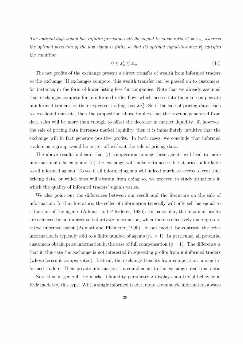
The optimal high signal has infinite precision with the signal-to-noise ratio x∗1 = xm, whereas

the optimal precision of the low signal is finite so that its optimal signal-to-noise x∗2 satisfies

the condition

0 ≤ x∗2 ≤ xm. (44)

The net profits of the exchange present a direct transfer of wealth from informed traders

to the exchange. If exchanges compete, this wealth transfer can be passed on to customers,

for instance, in the form of lower listing fees for companies. Note that we already assumed

that exchanges compete for uninformed order flow, which necessitate them to compensate

uninformed traders for their expected trading loss λσ2u. So if the sale of pricing data leads

to less liquid markets, then the proposition above implies that the revenue generated from

data sales will be more than enough to offset the decrease in market liquidity. If, however,

the sale of pricing data increases market liquidity, then it is immediately intuitive that the

exchange will in fact generate positive profits. In both cases, we conclude that informed

traders as a group would be better off without the sale of pricing data.

The above results indicate that (i) competition among these agents will lead to more

informational efficiency and (ii) the exchange will make data accessible at prices affordable

to all informed agents. To see if all informed agents will indeed purchase access to real time

pricing data, or which ones will abstain from doing so, we proceed to study situations in

which the quality of informed traders’ signals varies.

We also point out the differences between our result and the literature on the sale of

information. In that literature, the seller of information typically will only sell his signal to

a fraction of the agents (Admati and Pfleiderer, 1986). In particular, the maximal profits

are achieved by an indirect sell of private information, when there is effectively one represen-

tative informed agent (Admati and Pfleiderer, 1990). In our model, by contrast, the price

information is typically sold to a finite number of agents (n1 > 1). In particular, all potential

customers obtain price information in the case of full compensation (q = 1). The difference is

that in this case the exchange is not interested in squeezing profits from uninformed traders

(whose losses it compensated). Instead, the exchange benefits from competition among in-

formed traders. Their private information is a complement to the exchanges real time data.

Note that in general, the market illiquidity parameter λ displays non-trivial behavior in

Kyle models of this type. With a single informed trader, more asymmetric information always

20

leads to less liquidity. This is no longer the case when informed agents compete, since the

increase in competition is a counter-acting force. Thus, market liquidity is typically maximal

in market with either few or many informed agents. It is easy to see that an increase in the

price of information can have an ambiguous effect on λ.13

The assumption of the full compensation for the liquidity traders q = 1 is not realistic.

Indeed, the empirical evidence is that the liquidity traders on average loose money in the

trading process. We now consider general values of q ∈ [0; 1] for the rest of the paper. As

in Admati and Pfleiderer (1986), the exchange might opt to sell only a noisy version of the

most recent pricing data. We allow for this behavior and give conditions under which the

exchange indeed wants to add noise to the data it sells.

Therefore, we assume that the high types may receive a noisy price signal with the pre-

cision µp,1, while the low types receive a price signal with a lower precision µp,2 < µp,1. To

simplify the analysis, we first consider a limit when the precision of the delayed signal is

zero, µp,2 = 0, and therefore the signal-to-noise ratio in the low state is zero, x2 = 0. This

is not very unrealistic since the speculative value of the ”free” delayed signal is expected to

be small. According to (16), the payoff of each high type agent is

πh =1√n1

√x1

√1 + x1

1 + n1x1

, (45)

with x1 given by

x1 =

(1 +

2

µ2s

+2

µ2p,1

)−1

, (46)

and the low types make no profit, πl = 0. Therefore, the objective function of the exchange

is given by

Lq = (1− q)√

n1

√x1

√1 + x1

1 + n1x1

. (47)

It is easy to see that the objective function (47) is non-monotonic in the effective “signal-

to-noise ratio” parameter x1. As we show in the Appendix, the function (47) achieves its

maximum at

x∗n =1

n− 2. (48)

Since the parameter x1 given by (46) is limited by the precision of the private signal

x1 ≤ xc =

(1 +

2

µ2s

)−1

, (49)

13I have moved the above paragraph here. It used to be before Theorem; did not seems to make sense.

21

the precision of the price signal that the exchange sells depends on the relation between (48)

and (49). We obtain the following

Proposition 5. When all traders have the same precision of private information, the ex-

change sells a single price signal with infinite precision (real time price data) to all traders

if the number of traders is smaller than the critical number, n ≤ nc, and to a limited number

of nc traders if n ≥ nc, where the critical number is given by nc = 1 + 2µ2

s.

Note that the above result holds for any q ∈ [0; 1] provided that x2 = 0. In the case

of partial compensation q ∈ (0; 1), the exchange maximizes profits by setting the price of

information, c, such that a finite number n∗ ≤ n of informed agents in the economy purchase

information. The optimal number n∗ depends on the compensation ratio q and on signal to

noise parameters x1 and x2. In particular, there exist the bounds 0 < qc < 1 and qc < qm < 1

such that n∗ = 1 for q ∈ (qc; qm), and 1 < n∗ < n for q ∈ (0; qc).

The typical case is represented in Fig.2, where we present a two-dimensional contour

plot of the exchange objective function Lq (n1) as a function of the compensation parameter

q ∈ [0; 1] and the number of high type agents n1. The total number of informed agents is

n = 1000 and the high price signal has a precision µp,1 = 10. As can be seen in Fig.2, the

critical value in this case is qc ' 0.6.

4 Multiple Informed Traders with Heterogeneous Precision

We now analyze the general case in which agents have different precision of information, and

the exchange can sell signals of different quality. The insider i’s payoff is characterized by

ηi =π∗i (µ)

πK

= D (x)(xi + x2

i

). (50)

Using the scaled variables ηi, we obtain the following

Proposition 6. Agents with more precise private information (smaller σε,i) value accurate

price information more in the sense that they have a higher marginal utility of price infor-

mation.

The above proposition is consistent with the observation that the primary beneficiaries

of real-time price information are well-informed traders and large sophisticated financial

22

institutions. However, our result raises the following concern. If agents who already have

superior private information benefit more from real time price information, then granting

those agents access to price information might significantly increase the degree of information

asymmetry in the market, and therefore deteriorate market liquidity. We analyze this issue

below and confirm that it is indeed the case.

Suppose the exchange introduces a cost schedule for the information that depends on its

precision. Let C (µp,i) denote the cost that informed agent i needs to incur in order to acquire

price information of precision µp,i. We assume that the cost increases in the precision. The

informed traders decide upon the optimal precision to acquire based on their marginal utility

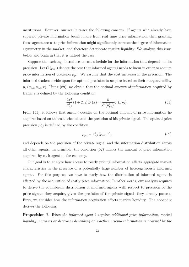
pµ (µp,i, µs,i, x). Using (89), we obtain that the optimal amount of information acquired by

trader i is defined by the following condition

2x2i

µ4p,i

(1 + 2xi) D (x) =∂

∂(µ2

p,i

)C (µP,i) . (51)

From (51), it follows that agent i decides on the optimal amount of price information he

acquires based on the cost schedule and the precision of his private signal. The optimal price

precision µ∗p,i is defined by the condition

µ∗p,i = µ∗p,i (µs,i, x) , (52)

and depends on the precision of the private signal and the information distribution across

all other agents. In principle, the condition (52) defines the amount of price information

acquired by each agent in the economy.

Our goal is to analyze how access to costly pricing information affects aggregate market

characteristics in the presence of a potentially large number of heterogeneously informed

agents. For this purpose, we have to study how the distribution of informed agents is

affected by the acquisition of costly price information. In other words, our analysis requires

to derive the equilibrium distribution of informed agents with respect to precision of the

price signals they acquire, given the precision of the private signals they already possess.

First, we consider how the information acquisition affects market liquidity. The appendix

derives the following:

Proposition 7. When the informed agent i acquires additional price information, market

liquidity increases or decreases depending on whether pricing information is acquired by the

23

agents on the left or on the right side of the distribution. The acquisition of price information

increases (decreases) market liquidity, if agent i’s informativeness, as measured by xi, is below

(above) the critical value xe = x + V ar(x)x

+ 12.

Here, x = E(xi) denotes the sample mean of the signal to noise ratio xi. The above result

implies that the price information acquired by informed traders, affects market liquidity in

an ambiguous way. For an individual informed agent acquiring the price information, the

effect on market liquidity depends on the amount of information the agent already possesses

represented by xi. If the agent’s ex-ante information is already above the critical value xe,

then the additional information on current price obtained by the agent increases the inverse

market depth, λ, and thus decreases market liquidity. If the agent’s signal to noise ratio

is below xe, the opposite occurs. Equation (94) shows that the critical value xe depends

on the sample average of all agents’ signal-to-noise ratios plus a shift proportional to the

sample variance. A simple intuition lies behind our finding. On the one hand, if the highly

informed agents become even more informed, the information asymmetry in the market

increases, leading to the reduction of the market liquidity. On the other hand, if the less

informed agents become more informed, the information asymmetry decreases and therefore

the market liquidity increases.

Together, propositions 6 and 7 define an interesting economic tension for the exchange as

seller of pricing data. While the sale of real time data to privately well-informed agents is

particularly profitable, the liquidity implications of doing so are problematic. Thus, optimal

sale of data in the presence of heterogeneously informed traders becomes a far more complex

problem to study. We proceed with the case of a binary distribution in agents’ precision of

private information before we analyze the general case.

4.1 Binary distribution of private precision

In order to analyze the equilibrium acquisition of price information, we first examine the

case of a binary distribution of the precision of agents’ private information. Agents either

have a high precision of µs,1 or a lower precision of µs,2 < µs,1. We assume that there are

n1 agents of type one and n2 agents of type two 14. Suppose that the exchange can sell two

14Note that the signals obtained by diferent agents are uncorrelated.

24

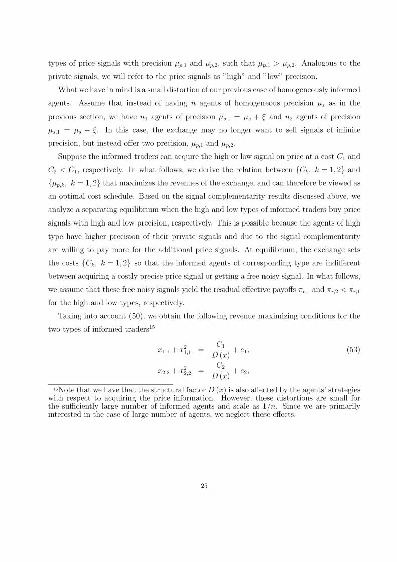
types of price signals with precision µp,1 and µp,2, such that µp,1 > µp,2. Analogous to the

private signals, we will refer to the price signals as ”high” and ”low” precision.

What we have in mind is a small distortion of our previous case of homogeneously informed

agents. Assume that instead of having n agents of homogeneous precision µs as in the

previous section, we have n1 agents of precision µs,1 = µs + ξ and n2 agents of precision

µs,1 = µs − ξ. In this case, the exchange may no longer want to sell signals of infinite

precision, but instead offer two precision, µp,1 and µp,2.

Suppose the informed traders can acquire the high or low signal on price at a cost C1 and

C2 < C1, respectively. In what follows, we derive the relation between Ck, k = 1, 2 and

µp,k, k = 1, 2 that maximizes the revenues of the exchange, and can therefore be viewed as

an optimal cost schedule. Based on the signal complementarity results discussed above, we

analyze a separating equilibrium when the high and low types of informed traders buy price

signals with high and low precision, respectively. This is possible because the agents of high

type have higher precision of their private signals and due to the signal complementarity

are willing to pay more for the additional price signals. At equilibrium, the exchange sets

the costs Ck, k = 1, 2 so that the informed agents of corresponding type are indifferent

between acquiring a costly precise price signal or getting a free noisy signal. In what follows,

we assume that these free noisy signals yield the residual effective payoffs πr,1 and πr,2 < πr,1

for the high and low types, respectively.

Taking into account (50), we obtain the following revenue maximizing conditions for the

two types of informed traders15

x1,1 + x21,1 =

C1

D (x)+ e1, (53)

x2,2 + x22,2 =

C2

D (x)+ e2,

15Note that we have that the structural factor D (x) is also affected by the agents’ strategieswith respect to acquiring the price information. However, these distortions are small forthe sufficiently large number of informed agents and scale as 1/n. Since we are primarilyinterested in the case of large number of agents, we neglect these effects.

25

with ek = πr,1/D (x) , k = 1, 2, and

x1,1 =

(1 +

2

µ2s,1

+2

µ2p,1

)−1

, (54)

x2,2 =

(1 +

2

µ2s,2

+2

µ2p,2

)−1

.

The incentive compatibility conditions take the form

x1,2 + x21,2 ≤ C2

D (x)+ e1, (55)

x2,1 + x22,1 ≤ C1

D (x)+ e2,

where

x1,2 =

(1 +

2

µ2s,1

+2

µ2p,2

)−1

, (56)

x2,1 =

(1 +

2

µ2s,2

+2

µ2p,1

)−1

.

Intuitively, the conditions (55) ensure that it is indeed optimal for the agent with high

precision of private information to acquire the high precision signal on price and vice versa,

thus ensuring a separating equilibrium. Solving (53), we obtain the following relation

µ2p,1

µ2p,2

=

(√14

+ C2

D(x)+ e2 − 1

2

)−1

− 1− 2µ2

s,2(√14

+ C1

D(x)+ e1 − 1

2

)−1

− 1− 2µ2

s,1

. (57)

With the notations ∆Ck = Ck

D(x)− ek, k = 1, 2, and y = ∆C1/∆C2, (57) finally yields

µ2p,1

µ2p,2

= Θ (y) , (58)

Θ (y) = y

√14

+ C2

D(x)+ e2 + 1

2−

(1 + 2

µ2s,2

)∆C2

√14

+ y∆C2 + 2e1 + 12− y

(1 + 2

µ2s,1

)∆C2

.

Analogously, solving (55), we obtain the conditions

Ω

(C1

D

)≤ 0, (59)

Ω

(C2

D

)≥ 0,

26

with

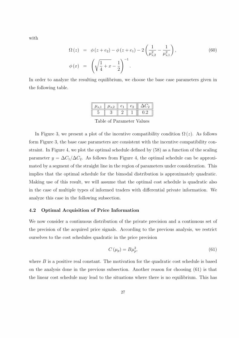
Ω (z) = φ (z + e2)− φ (z + e1)− 2

(1

µ2s,2

− 1

µ2s,1

), (60)

φ (x) =

(√1

4+ x− 1

2

)−1

.

In order to analyze the resulting equilibrium, we choose the base case parameters given in

the following table.

µs,1 µs,2 e1 e2

5 3 2 1

∆C2

0.2

Table of Parameter Values

In Figure 3, we present a plot of the incentive compatibility condition Ω (z). As follows

form Figure 3, the base case parameters are consistent with the incentive compatibility con-

straint. In Figure 4, we plot the optimal schedule defined by (58) as a function of the scaling

parameter y = ∆C1/∆C2. As follows from Figure 4, the optimal schedule can be approxi-

mated by a segment of the straight line in the region of parameters under consideration. This

implies that the optimal schedule for the bimodal distribution is approximately quadratic.

Making use of this result, we will assume that the optimal cost schedule is quadratic also

in the case of multiple types of informed traders with differential private information. We

analyze this case in the following subsection.

4.2 Optimal Acquisition of Price Information

We now consider a continuous distribution of the private precision and a continuous set of

the precision of the acquired price signals. According to the previous analysis, we restrict

ourselves to the cost schedules quadratic in the price precision

C (µp) = Bµ2p, (61)

where B is a positive real constant. The motivation for the quadratic cost schedule is based

on the analysis done in the previous subsection. Another reason for choosing (61) is that

the linear cost schedule may lead to the situations where there is no equilibrium. This has

27

a simple intuition, since the economics of a problem is defined in terms of the marginal cost

being a derivative of (61). In case of the linear cost schedule, the marginal cost is a constant,

which may lead to corner solutions of the optimization problem for the objective function of

the exchange.

Substituting the schedule (61) into (51), we obtain16

x2i

µ4p,i

(1 + 2xi) D (x) =B

2. (62)

Combining (51) and (15), we obtain the following equilibrium condition

Φ(µ2

p,i, µ2s,i

)= ε, (63)

with effective marginal benefit

Φ (ξ, η) = η2

(ξ + η + 3

2ξη

)(ξ + η + 1

2ξη

)3 . (64)

and cost schedule parameter

ε =2B

D (x). (65)

The relation (63) defines the precision of price signal µp,i acquired by the informed agent

with a precision of private signal µs,i.

Note that since the arguments of (64) represent precision, we are only interested in so-

lutions of (63) consisting of positive values of µS,i and µp,i. The pair of equations (63) and

(64) has positive solutions only if ε ∈ [0, 1]. Economically, this means that the equilibrium

cost schedule parameter has to be sufficiently small. Otherwise, the marginal cost and ben-

efits of acquiring the information are not be balanced, and there is no equilibrium. This

is illustrated in Figure 5, where the function Φ(µ2

p, µ2s

)is plotted against its arguments.

Clearly, Φ(µ2

p, µ2s

) ≤ 1 for positive values of µp and µs, and therefore (63) only has solutions

if ε ∈ [0, 1]. Figure 5 also illustrates an important signal complementarity property of our

model. Namely, the marginal benefit of information acquisition for agent i, Φ(µ2

p,i, µ2s,i

),

increases in the precision of his private signal µs,i. In other words, more informed agents

have higher marginal benefits for the additional price signal.

In Figure 6, we present solutions µp,i (µs,i, ε) of (63) for three values of the cost schedule

parameter ε = 2BD(x)

= 0.3, 0.5, 0.8. We observe that the traders with more private information

16See the previous footnote.

28

also buy a price signal with higher precision. This is consistent with Figure 5 and the results

of proposition 6. As the agents’ private precision goes to infinity, the precision of the acquired

information on price remains bounded, µp,i < µp,max (ε) < ∞. As it follows from Figure 6,

the upper bound µp,max (ε) decreases in the cost schedule parameter ε. This has a simple

intuition, since when the information on price becomes more costly, the agents are less willing

to purchase it. These results are summarized in

Proposition 8. When the exchange sells pricing information according to a quadratic cost

schedule, then an equilibrium exists if the cost schedule parameter ε is sufficiently low. The

equilibrium precision of the acquired signals decreases in the cost schedule parameter ε.

4.3 Equilibrium distribution of price precision

We study the equilibrium distribution of price precision acquired by informed traders. In

what follows, we show that the distribution is characterized by a continuous probability

density function (p.d.f.)17.

Since the function (64) can not be inverted analytically the closed form fully analytic

solutions are not available, and part of this work relies on numerical simulations.

We assume that the precision of private signals is uniformly distributed across the in-

formed agents with the finite support µs ∈ [0, µs max]. For the base case simulations, we

adopt µs max = 10. First we derive the p.d.f. ρ (µp) for the equilibrium distribution of the

acquired price signal µp. This p.d.f. is uniquely defined provided that there is a relation

µs = Γ (µp), and the function Γ (·) is monotonic. As is illustrated by Figure 6, this is indeed

the case. The details of the derivation are given in the appendix.

The p.d.f. is presented in Figure 7. The cost schedule parameter ε = 2BD(x)

is taken

17This does not contradict the fact that the total number N of agents in our model economyis finite (possibly large), and therefore their payoffs are non-zero. The reason is that accordingto (52), the amount of price information acquired by each informed agent is completelydefined by the precision of his private signal and the cost schedule parameter. In otherwords, (52) can be viewed as a mapping of private information distribution onto the resultingdistribution of price information. More specifically, this mapping is presented in Figure4. Note that for each realization of private information distribution, we can construct thecorresponding distribution of price information using the mapping (52). For finite number ofagents, each realization of the distribution of private information is represented by a discretedistribution of the precisions. However, the resulting distribution is continuous if we averageover the possible realizations of initial discrete distribution. This also reflects the ergodicityproperty of our model.

29

ε = 0.5. Dashed line illustrates the p.d.f. of the corresponding uniform distribution. As one

can see, the resulting p.d.f. ρ (µp) of the distribution of price precision has a finite support

µp ∈ [0, µp max] with µp max = 1.38. Also, the p.d.f. ρ (µp) is right-skewed in comparison to

the uniform one. The reason is the complementarity between the private and price signals in

our model, meaning that the agents with higher precision of their private signals also tend

to acquire more precise information on price. Therefore, the p.d.f. increases for the large

price precision. To summarize, we make the following observation. When the exchange sells

pricing information according to a quadratic cost schedule, then the equilibrium distribution

of the precision of the acquired signals is right-skewed. This is due to the complementarity

between the private signals and the signals on price.

From analysis of Figure 6 it also follows that the cost schedule parameter ε = 2BD(x)

is

uniquely defined given the distribution of the precision of private signals ρ (µp). Indeed, as it

follows from Figure 6, for each ε ∈ [0, 1] we can uniquely define the equilibrium distribution

of the precision of acquired price signals. From this distribution and making use of the

definition (50), we can derive the structural factor D (x), and therefore define the slope of

cost schedule B as

B (ε) =εD (x (ε))

2. (66)

As a result, we obtain a unique value of the slope B (ε) for each cost schedule parameter

ε. The results are presented in Figure 8. Importantly, the function B (ε) is monotonically

increasing and goes to infinity as ε → 1. This illustrates that the equilibrium exists for any

positive slope of the cost schedule B. Since the function B (ε) is monotonically increasing,

the inverse function ε = ε (B) is well defined. Therefore, the slope B uniquely defines

the equilibrium scaling parameter ε. Since the scaling parameter ε completely defines the

equilibrium distribution, it follows that the slope B also uniquely defines the equilibrium

distribution of the price precision.

In Figure 10, we present the inverse market depth parameter λ (ε) as a function of the

effective slope ε. Clearly, the inverse market depth monotonically decreases in ε and therefore

also monotonically decreases in the cost slope B. This has a simple intuition. As the

price information becomes more costly, less agents acquire the information and therefore the

information asymmetry decreases. In the limit when B goes to infinity, the agents do not

acquire any price information, their profits go to zero and therefore the liquidity losses go

30

to zero. In other words, in the limit when B →∞ we have λ (ε) → 0, and market becomes

infinitely deep.

One should note that when the effective slope increases, the support of the p.d.f. of price

precision distribution decreases and the ”bump” on the right tale of the distribution becomes

more narrow. This means that as the cost slope B increases, the average agent acquires less

price information. At the same time, when the slope is high, there is a small fraction of

highly informed agents who are still willing to acquire the information with a very high

precision. These agents contribute to the narrow and high peak on the right tale of Figure

7. However, the fraction of such agents is small and the information asymmetry decreases

as the cost slope increases.

The above results are summarized as follows. When the exchange sells pricing information

according to a quadratic cost schedule, the equilibrium exists for arbitrary non-zero slope B

of the cost schedule. As the slope B increases, the agents acquire less information on price,

their profits decrease, and the market liquidity increases.

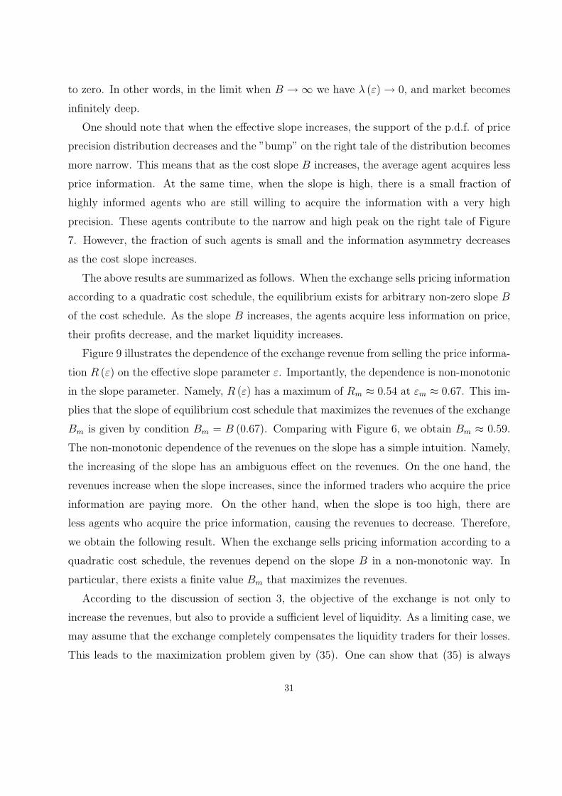
Figure 9 illustrates the dependence of the exchange revenue from selling the price informa-

tion R (ε) on the effective slope parameter ε. Importantly, the dependence is non-monotonic

in the slope parameter. Namely, R (ε) has a maximum of Rm ≈ 0.54 at εm ≈ 0.67. This im-

plies that the slope of equilibrium cost schedule that maximizes the revenues of the exchange

Bm is given by condition Bm = B (0.67). Comparing with Figure 6, we obtain Bm ≈ 0.59.

The non-monotonic dependence of the revenues on the slope has a simple intuition. Namely,

the increasing of the slope has an ambiguous effect on the revenues. On the one hand, the

revenues increase when the slope increases, since the informed traders who acquire the price

information are paying more. On the other hand, when the slope is too high, there are

less agents who acquire the price information, causing the revenues to decrease. Therefore,

we obtain the following result. When the exchange sells pricing information according to a

quadratic cost schedule, the revenues depend on the slope B in a non-monotonic way. In

particular, there exists a finite value Bm that maximizes the revenues.

According to the discussion of section 3, the objective of the exchange is not only to

increase the revenues, but also to provide a sufficient level of liquidity. As a limiting case, we

may assume that the exchange completely compensates the liquidity traders for their losses.

This leads to the maximization problem given by (35). One can show that (35) is always

31

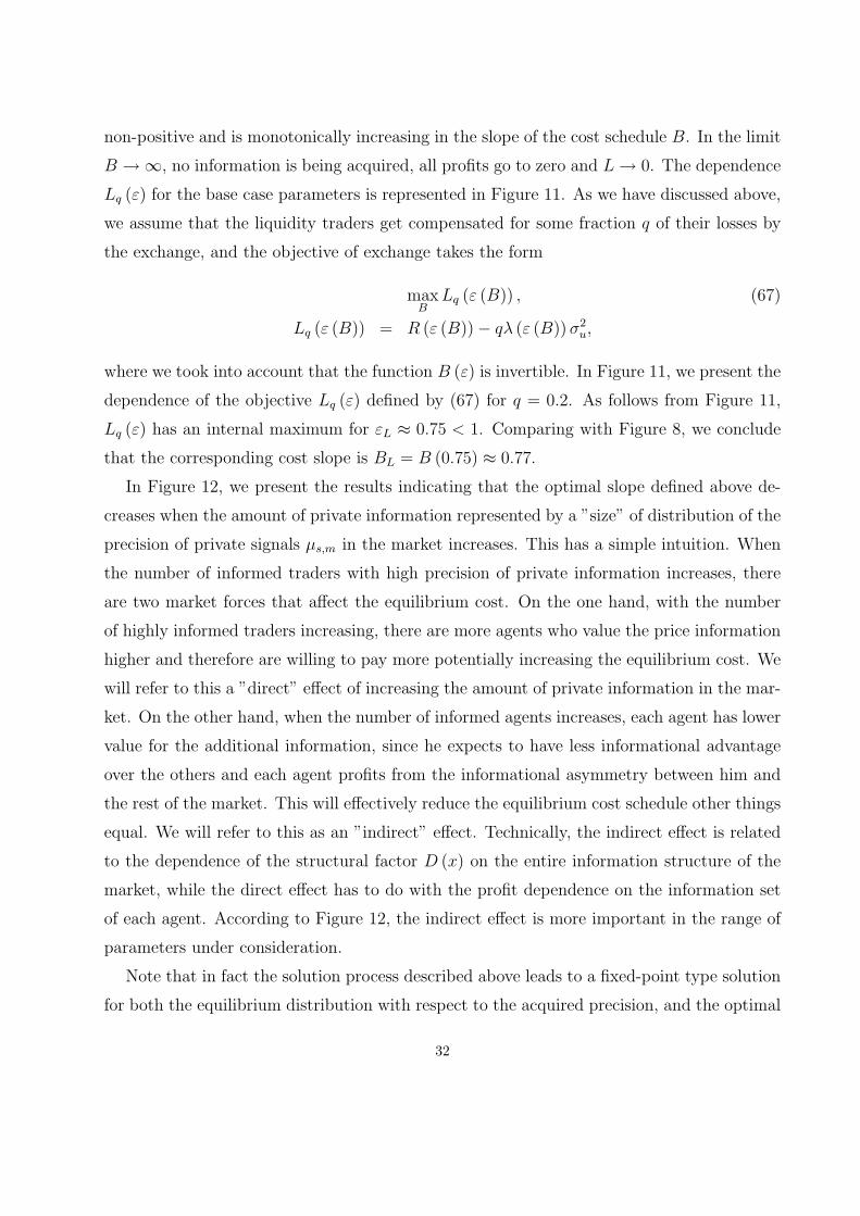
non-positive and is monotonically increasing in the slope of the cost schedule B. In the limit

B →∞, no information is being acquired, all profits go to zero and L → 0. The dependence

Lq (ε) for the base case parameters is represented in Figure 11. As we have discussed above,

we assume that the liquidity traders get compensated for some fraction q of their losses by

the exchange, and the objective of exchange takes the form

maxB

Lq (ε (B)) , (67)

Lq (ε (B)) = R (ε (B))− qλ (ε (B)) σ2u,

where we took into account that the function B (ε) is invertible. In Figure 11, we present the

dependence of the objective Lq (ε) defined by (67) for q = 0.2. As follows from Figure 11,

Lq (ε) has an internal maximum for εL ≈ 0.75 < 1. Comparing with Figure 8, we conclude

that the corresponding cost slope is BL = B (0.75) ≈ 0.77.

In Figure 12, we present the results indicating that the optimal slope defined above de-

creases when the amount of private information represented by a ”size” of distribution of the

precision of private signals µs,m in the market increases. This has a simple intuition. When

the number of informed traders with high precision of private information increases, there

are two market forces that affect the equilibrium cost. On the one hand, with the number

of highly informed traders increasing, there are more agents who value the price information

higher and therefore are willing to pay more potentially increasing the equilibrium cost. We

will refer to this a ”direct” effect of increasing the amount of private information in the mar-

ket. On the other hand, when the number of informed agents increases, each agent has lower

value for the additional information, since he expects to have less informational advantage

over the others and each agent profits from the informational asymmetry between him and

the rest of the market. This will effectively reduce the equilibrium cost schedule other things

equal. We will refer to this as an ”indirect” effect. Technically, the indirect effect is related

to the dependence of the structural factor D (x) on the entire information structure of the

market, while the direct effect has to do with the profit dependence on the information set

of each agent. According to Figure 12, the indirect effect is more important in the range of

parameters under consideration.

Note that in fact the solution process described above leads to a fixed-point type solution

for both the equilibrium distribution with respect to the acquired precision, and the optimal

32

cost schedule set by the exchange. Indeed, we first define the functional form of the distribu-

tion of the precision, which depends on both the slope of the cost schedule B and the higher

moments of the distribution itself contained in the structural factor D (x). Then we choose

the parameter of the distribution in order to match the structural factor D (x) and the slope

B. When this is done, we effectively ”close the loop” and make the solution self-consistent,

i.e. the true equilibrium. We also define both equilibrium structural factor D (x) and the

slope of the cost schedule Beq optimal for the exchange.

Technically, the solution of such two-dimensional fixed point problem could be a difficult

task, especially since one of the ”variables” is actually a function D (x). The reason why this

is feasible in our case is that the solution actually depends only on a combination ε = 2BD(x)

,

which means that we have a special ”scaling property” in this model. For this reason,

the fixed-point problem becomes essentially one-dimensional and therefore more tractable.

However, it still requires extensive numerical simulations.

5 Conclusion and Extensions

Agents who want access to real time price quotes pay considerable amounts for this service.

This fee can range from a nominal amount for private accounts up to hundreds of thousands of

dollars annually for the most reliable and comprehensive service from Reuters or Bloomberg.

We derive the “price of prices” in a Kyle-type setting where we explicitly account for the

fact that in the U.S., exchanges have property rights in the price quotes they generate. In

the process, we document the beneficial welfare effects of granting individuals access to real-

time pricing data (such as an increase in price informativeness). Since doing so may impact

market liquidity in a detrimental way, the exchange needs to charge for this service.

When informed agents have equal precision of private information, and the exchange

takes the liquidity impact of data sales on uninformed traders fully into account, we show

the following. The exchange finds it optimal to sell a high precision signal (often of infinite

precision) to informed traders. Due to the impact of data sales on liquidity, the exchange

typically needs to charge for this service, and informed traders are willing to acquire it. We

also provide conditions under which the exchange benefits when a second, lower precision

signal is made publicly available. We interpret the first behavior as the sale of real time

33

pricing data, while the second action corresponds to the free dissemination of a noisy signal

of current price as in the publication of delayed price quotes. Empirical evidence shows that

the speculative value of public information is greatly diminished after 5 to 15 minutes. This

might possibly explain why U.S. exchanges delay free quotes by 10 to 30 minutes.

Roll (1984) has shown that prices contain substantial amounts of useful information. We

follow Grossman and Stiglitz (1980) in postulating that the value of this information to

traders is best measured by agents’ willingness to pay for it. We observe that the major

exchanges receive substantial amounts of their revenue from data sales. This allows us to

conclude that the information content of market prices is of an economically significant

magnitude. Our aim is to provide a simple model that explains the price of prices and to

understand the economics of the sale of real time price data by exchanges such as the NYSE.

Our model has several empirical implications.

Our analysis suggests that the price of prices is intimately related to the amount and

extent of informed trading in a market. We predict that the price of prices is higher in

markets in which more private information is present, as real time price information acts

as a complement to private information. A measure such as the probability of informed

trade, PIN, endeavors to capture what we are after. Note, however, that PIN is a relative

measure of the percentage of informed trades, while we consider the absolute amount, so we

would need to consider the multiple of PIN by trading volume. This reasoning implies that

a market with substantial informed trading will have a significant price of prices. This might

explain both the high price of real time data access and the significant amount of revenue

produced by a major exchange such as the NYSE. Conversely, exchanges with less informed

trade have a lower price of prices. For instance, one might compare markets for different

securities. We conjecture that privately informed trading is less pronounced in bond markets

(due to the bonds’ concave pay-offs and lower market liquidity), our theory predicts that the

price of prices is lower in such markets.

One of the most interesting aspects of the delay times reported in table 1 is the variation

within Chinese markets. The mainland Chinese exchanges in Shanghai and Shenzhen provide

price quotes for free. Hong Kong, on the other hand, has the longest delay in the sample,

60 minutes. We conjecture that a substantial amount of price discovery and informed trade

takes place at Hong Kong, where market liquidity is greater. Thus, the price of prices may

34

be more significant here. And while we do not claim that we can explain the differences

completely, our results do indicate that even free disclosure of real time price information is

in the interest of an exchange. If the expected revenue from selling real time data is low,

then the exchange may abstain from doing so.

Our analysis in section 4 makes the interaction between the amount of private information

and the price of prices more precise. Specifically, we show that the slope of the optimal cost

schedule is indeed decreasing in the amount of private information in the market. Given

the right data, this could lead to a more specific empirical test of our model. We show that

the exchange typically finds it optimal to sell pricing information to a significant number of

informed traders. In particular, real time price data is sold to all informed agents when the

precision of their information is equal and uninformed traders are sufficiently compensated

for their losses. In general, we find that it is the better informed agents who acquire more

precise pricing information. This seems to coincide with our beliefs of which agents do

purchase real time pricing data through services such as Bloomberg or Reuters. But it could

certainly be tested given micro-level data.

Another interesting dimension of the price of prices is variations within a single exchange.

As aforementioned, the NYSE offers a substantial discount to customers who are willing to

accept a 5 second delay in prices. This can be explained by our model. As shown in section 4,

when information precision differs across agents, the privately better informed ones purchase

considerably more pricing information even in the presence of a super-linear price schedule

such as a quadratic. Since the difference in precision of price information between a zero and

a five second delay is very significant, we can rationalize a substantial price difference. Our

result critically depends on competition among informed traders, which puts the purchaser

of even marginally delayed information at a significant disadvantage. Modelling the specific

dynamics of informed trade that enable us to say more about different periods of delay

remains an interesting opportunity for further work.

Several interesting aspects remain to be explored in future research. On the one hand, one

could analyze the role of liquidity providers and market making more explicitly. Certainly,

institutions which attempt to create or unwind significant asset positions will benefit from

observing current market demand by subscribing to real time prices. Alternatively, in a model

of imperfect competition among market makers, each market maker may obtain information

35

about order flow directed to other market makers through real time price access. This will be

an interesting direction for future research. On the other hand, one could envision a model

with richer, more complex dynamic trading strategies. For instance, the model of Back, Cao

and Willard (2000) could be extended to allow for different classes of agents: some receive

real time price access and some do not. Doing so will yield interesting insights into the price

of prices, but will probably come at a hefty analytical expense.

36

References

Admati, A., and P. Pfleiderer, 1986, “A Monopolistic Market for Information”, Journal of EconomicTheory 39, 400-438.

Admati, A., and P. Pfleiderer, 1988, “ A Theory of Intraday Patterns: Volume and Price Variability”,Review of Financial Studies 1, 3-40.

Admati, A., and P. Pfleiderer, 1990, “Direct and Indirect Sale of Information”, Econometrica 58, 901-928.Back, K., Cao, H., and G. Willard, 2000, Imperfect Competition among Informed Traders,Journal of

Finance 55, 2117u2155.Barclay, M., and R. Litzenberger, 1988, “Announcement Effects of New Equity Issues and the Use of

Intraday Price Data”, Journal of Financial Economics 21, 71-99.Busse, J., and C. Green, 2002, “Market Efficiency in Real Time”, Journal of Financial Economics 65,

415-438.Cochrane, J., “Asset Pricing”, revised edition, Princeton University Press, Princeton 2005.Grossman, S., and J. Stiglitz, 1980, “On the Impossibility of Informationally Efficient Markets”, American

Economic Review 70, 393-408.Holmstrom, B., and J. Tirole, 1993, “Market Liquidity and Performance Monitoring”, Journal of Political

Economy 101, 678-709.Huang, C., and R. Litzenberger, “Foundations for Financial Economics”, Elsevier Science Publishing,

New York, 1988.Huddart, S., J. Hughes, and M. Brunnermeier, 1999, “Disclosure Requirements and Stock Listing Choices

in and International Context”, Journal of Accounting and Economics 26, 237-269.Jennings, R., and L. Starks, 1985, “Information Content and the Speed of Stock Price Adjustment”,

Journal of Accounting Research 23, 336-350.Kandel, E., and N. Pearson, 1995, “Differential Interpretation of Public Signals and Trade in Speculative

Markets,” Journal of Political Economy 103, 831-872.Kim, S., J. Lin, and M. Slovin, 1997, “Market Structure, Informed Trading, and Analyst Recommenda-

tions”, Journal of Financial and Quantitative Analysis 32, 507-524.Kyle, A., 1985, “Continuous Auctions and Insider Trading”, Econometrica 53, 1315-1335.Mulherin, H., J. Netter, and J. Overdahl, 1991, “Prices are Property: The Organization of Financial

Exchanges from a Transaction Cost Perspective”, Journal of Law and Economics 34, 591-644.Patell, J., and M. Wolfson, 1984, “The Intraday Speed of Adjustment of Stock Prices to Earnings and

Dividend Announcements, Journal of Financial Economics 13, 223-252.Roll, R., 1984, “Orange Juice and Weather”, American Economic Review 74, 861-880.

37

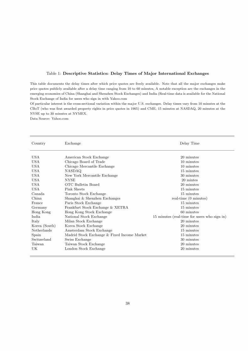
Table 1: Descriptive Statistics: Delay Times of Major International Exchanges

This table documents the delay times after which price quotes are freely available. Note that all the major exchanges make

price quotes publicly available after a delay time ranging from 10 to 60 minutes, A notable exception are the exchanges in the

emerging economies of China (Shanghai and Shenzhen Stock Exchanges) and India (Real-time data is available for the National

Stock Exchange of India for users who sign in with Yahoo.com

Of particular interest is the cross-sectional variation within the major U.S. exchanges. Delay times vary from 10 minutes at the

CBoT (who was first awarded property rights in price quotes in 1905) and CME, 15 minutes at NASDAQ, 20 minutes at the

NYSE up to 30 minutes at NYMEX.

Data Source: Yahoo.com

Country Exchange Delay Time

USA American Stock Exchange 20 minutesUSA Chicago Board of Trade 10 minutesUSA Chicago Mercantile Exchange 10 minutesUSA NASDAQ 15 minutesUSA New York Mercantile Exchange 30 minutesUSA NYSE 20 mintesUSA OTC Bulletin Board 20 minutesUSA Pink Sheets 15 minutesCanada Toronto Stock Exchange 15 minutesChina Shanghai & Shenzhen Exchanges real-time (0 minutes)France Paris Stock Exchange 15 minutesGermany Frankfurt Stock Exchange & XETRA 15 minutesHong Kong Hong Kong Stock Exchange 60 minutesIndia National Stock Exchange 15 minutes (real-time for users who sign in)Italy Milan Stock Exchange 20 minutesKorea (South) Korea Stock Exchange 20 minutesNetherlands Amsterdam Stock Exchange 15 minutesSpain Madrid Stock Exchange & Fixed Income Market 15 minutesSwitzerland Swiss Exchange 30 minutesTaiwan Taiwan Stock Exchange 20 minutesUK London Stock Exchange 20 minutes

38

6 Appendix: Proofs

Proof of Proposition 1The expected payoff of agent i is given by

πi = Et

[βi

(Si − Pi

)(V − P − λβi

(Si − Pi

))], (68)

with

P = V + σδ εδ, (69)Si = V + σs,iεs,i,

Pi = P + σp,iεp,i.

Here, εδ, εs,i and εp,i are standard Normal random variables. Assuming that all signals are uncorrelated,we obtain

πi = βiσ2δ

1− λβi

σ2δ + σ2

η,i + σ2ε,i

σ2δ

− λ∑

j 6=i

βj

. (70)

The FOC applied to (70) yields

βi =12λ

σ2δ

σ2δ + σ2

η,i + σ2ε,i

1− λ

∑

j 6=i

βj

. (71)

Solving (71), we obtain

βi =1− λq

λ

σ2δ

σ2δ + σ2

η,i + σ2ε,i

, (72)

with

q =1λ

11 + f

, (73)

f =n∑

j=1

σ2δ

σ2δ + 2σ2

η,i + 2σ2ε,i

.

Since the losses of liquidity traders equal the aggregate payoffs of the informed agents, the he liquidityparameter λ satisfies

λσ2u =

σ2δ

λ

g

(1 + f)2, (74)

g =n∑

j=1

(σ2

δ

σ2δ + 2σ2

η,i + 2σ2ε,i

)2

.

Combining (72), (73) and (74), we obtain, the results of the proposition.Q.E.D.

Proof of Proposition 2Proposition 2 simply follows from proposition 1 by setting the number of informed traders in period t,

nt, equal to one. Then we compare the single informed traders expected payoff π1,t depending on whetherhe acquires pricing information or not. The difference is found to be always positive and is denoted as δt inproposition 2. With a single informed trader, any additional profits he makes need to come at the expense of

39

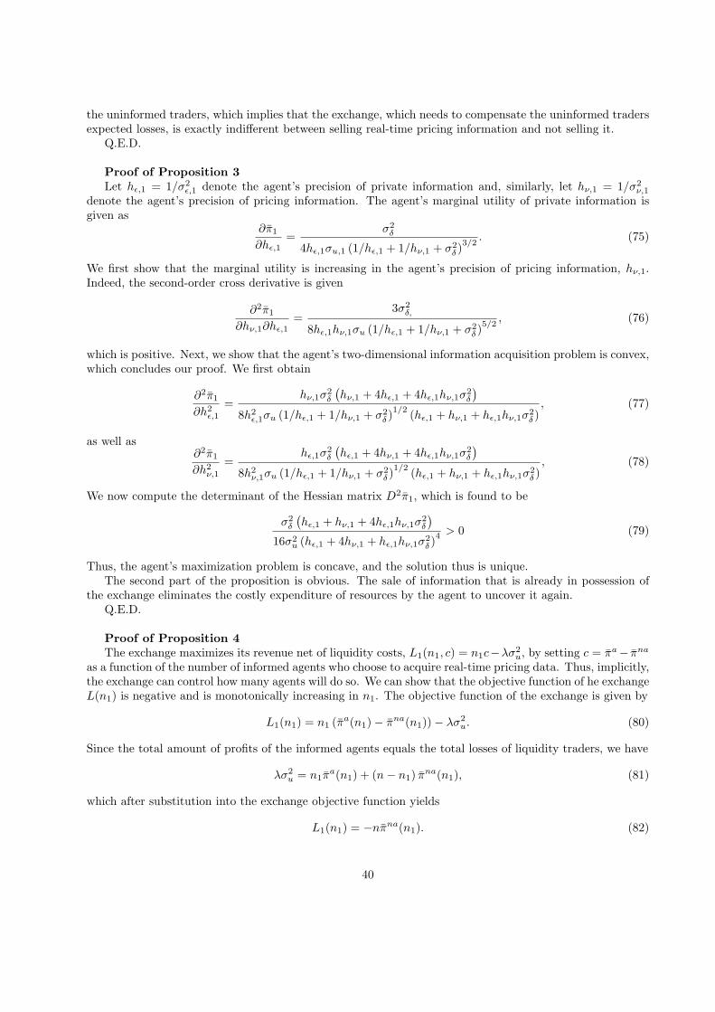
the uninformed traders, which implies that the exchange, which needs to compensate the uninformed tradersexpected losses, is exactly indifferent between selling real-time pricing information and not selling it.

Q.E.D.

Proof of Proposition 3Let hε,1 = 1/σ2

ε,1 denote the agent’s precision of private information and, similarly, let hν,1 = 1/σ2ν,1

denote the agent’s precision of pricing information. The agent’s marginal utility of private information isgiven as

∂π1

∂hε,1=

σ2δ

4hε,1σu,1 (1/hε,1 + 1/hν,1 + σ2δ )3/2

. (75)

We first show that the marginal utility is increasing in the agent’s precision of pricing information, hν,1.Indeed, the second-order cross derivative is given

∂2π1

∂hν,1∂hε,1=

3σ2δ,

8hε,1hν,1σu (1/hε,1 + 1/hν,1 + σ2δ )5/2

, (76)

which is positive. Next, we show that the agent’s two-dimensional information acquisition problem is convex,which concludes our proof. We first obtain

∂2π1

∂h2ε,1

=hν,1σ

2δ

(hν,1 + 4hε,1 + 4hε,1hν,1σ

2δ

)

8h2ε,1σu (1/hε,1 + 1/hν,1 + σ2

δ )1/2 (hε,1 + hν,1 + hε,1hν,1σ2δ )

, (77)

as well as∂2π1

∂h2ν,1

=hε,1σ

2δ

(hε,1 + 4hν,1 + 4hε,1hν,1σ

2δ

)

8h2ν,1σu (1/hε,1 + 1/hν,1 + σ2

δ )1/2 (hε,1 + hν,1 + hε,1hν,1σ2δ )

, (78)

We now compute the determinant of the Hessian matrix D2π1, which is found to be

σ2δ

(hε,1 + hν,1 + 4hε,1hν,1σ

2δ

)

16σ2u (hε,1 + 4hν,1 + hε,1hν,1σ2

δ )4> 0 (79)

Thus, the agent’s maximization problem is concave, and the solution thus is unique.The second part of the proposition is obvious. The sale of information that is already in possession of

the exchange eliminates the costly expenditure of resources by the agent to uncover it again.Q.E.D.

Proof of Proposition 4The exchange maximizes its revenue net of liquidity costs, L1(n1, c) = n1c−λσ2

u, by setting c = πa− πna

as a function of the number of informed agents who choose to acquire real-time pricing data. Thus, implicitly,the exchange can control how many agents will do so. We can show that the objective function of he exchangeL(n1) is negative and is monotonically increasing in n1. The objective function of the exchange is given by

L1(n1) = n1 (πa(n1)− πna(n1))− λσ2u. (80)

Since the total amount of profits of the informed agents equals the total losses of liquidity traders, we have

λσ2u = n1π

a(n1) + (n− n1) πna(n1), (81)

which after substitution into the exchange objective function yields

L1(n1) = −nπna(n1). (82)

40

From (32) with (33), it follows that πna(n1) monotonically decreases in n1. Therefore, the objective function(82) is maximized by the maximal value of n1 = n. The optimal value of (82) is therefore

L∗1 = L1 (n) = −nπna(n). (83)

Combining (83) with (33) and substituting into (36), we obtain the second result of the proposition. Theoptimal profits are positive since x1 ≥ x2.

It is straightforward to show that price informativeness in the market is higher with all agents acquir-ing price information (the equilibrium strategy for the exchange) as opposed to no agent acquiring priceinformation.

Q.E.D.

Proof of Corollary 1Follows from the text.Q.E.D.

Proof of Proposition 5Differentiating (47) with respect to x1, we obtain the FOC

(x1 +

12

)(1 + n1x1)− n1x1 (1 + x1) = 0, (84)

which has a unique solution

x∗1 =1

n1 − 2. (85)

Taking into account (49), we conclude that (85) holds if the number of high type agents is sufficiently large

n1 ≥ nc + 2 = 3 +2µ2

s

. (86)

If (86) does not hold, the optimal precision of the price signal is infinite. Summarizing the above, we have

x∗1 =1

n1 − 2, n1 ≥ nc + 2, (87)

x∗1 =1nc

, n1 ≤ nc + 2.

Note that the difference between our result and the corresponding one parallel to (Admati and Pfleiderer,1990) is that our critical number contains an extra term proportional to the inverse relative private precision2

µ2s, which vanishes in the limit of infinite precision of private information, but may be quite large for

sufficiently low private precision. Taking (85) and (86) into account and combining with (47), we obtain theobjective of the exchange optimized with respect to the precision of the price signal, in the form

Q.E.D.

Proof of Proposition 6The marginal value of the information for the i-th informed trader is given by

∂ηi

∂si=

∂ηi

∂xi

∂xi

∂si,

∂xi

∂si= −2x2

i ≤ 0.

41

Following the setting of the previous subsection, the marginal value of the price information for the k-thinformed trader is given by

p (si, zi, x) =∂ηi

∂si= −2x2

i (1 + 2xi)D (x) . (88)

Since µp,i = 1si

and µs,i = 1zi

, the marginal value is also defined in terms of signal precision, in the form

pµ (µp,i, µs,i, x) =∂ηi

∂µp,i= −

(1

µp,i

)2∂ηi

∂si(89)

=2x2

i

µ2p,i

(1 + 2xi) D (x) .

Note that (88) is obtained by the partial differentiation of (50) and taking into account that the ”structuralfactor” D (x) only depends on the information distribution across the agents, and not on the actions of aparticular agent. This is consistent with the optimization scheme of the previous subsection, where theagents’ willingness to pay was defined by comparing their expected payoffs in the states with the high andlow information quality assuming that the distribution of the information (characterized in that case only bya number of the agents in a high information state n1) is not affected by the actions of the informed agent.We also have

∂ηi

∂µp,i=

∂ηi

∂xi

∂xi

∂µp,i,

∂xi

∂µp,i= 2µ2

p,ix2i ≥ 0,

∂xi

∂µs,i= 2µ2

s,ix2i ≥ 0.

Differentiating the marginal profits with respect to the precision of the private signal µs,i and taking intoaccount that the structural factor D (x) does not change, we obtain

Ji =∂2ηi

∂µs,i∂µp,i= 4µ2

p,iµ2s,iD (x) x2

i

∂

∂xi

(x2

i (1 + 2xi))

(90)

= 8µ2p,iµ

2s,iF (x) x3

i (1 + 3xi) ≥ 0,

implying that the marginal profits of the informed traders with respect to the price precision increase in theprecision of their private signals.

Q.E.D.

Proof of Proposition 7Making use of (12), we obtain

∂λ

∂µi= 2x2

i s2i

∂λ

∂xi, (91)

∂λ

∂xi=

1√2β0

(12

1 + 2xi

(1 + f)√

f + g−√

f + g

(1 + f)2

).

From (91), it follows that

∂λ

∂µi≥ 0, xi ≥ xe, (92)

∂λ

∂µi≤ 0, xi ≤ xe,

42

where

xe =12f (x) + g (x)− 1

2

1 + f (x). (93)

Recalling the definition of f (x) and g (x) from (50), we obtain from (93) in the large-N limit

xe =12

+x2

x= x +

V ar (x)x

+12, (94)

with

x =f (x)

n=

1n

n∑

j=1

xj , (95)

x2 =g (x)

n=

1n

n∑

j=1

x2j .

Combining (92) and (94), we finally arrive at

∂λ

∂µi≥ 0, xi ≥ x +

V ar (x)x

+12, (96)

∂λ

∂µi≤ 0, xi ≤ x +

V ar (x)x

+12.

Q.E.D.

Proof of Proposition 8Follows immediately from the text.Q.E.D.

Proof of Proposition 9Since the p.d.f. ρs (µs) of the precision of private signals across the agents is uniform, we have for the

p.d.f. of the precision of price signals across the agents ρp (µp)

ρp (µp) = ρs (µs (µp))dµs (µp)

dµp(97)

= ρs (Γ (µp))dΓ (µp)

dµp,

with the function Γ (µp) defined from the equilibrium condition (63), as an isolevel curve of the function(64). Differentiating (64), we obtain

dΓ (µ)dµ

=Γ3 (µ)

µ2

m1

m2m3 −m4, (98)

where

m1 = µ + Γ (µ) + 2µΓ (µ) , (99)

m2 = µ + Γ (µ) +32µΓ (µ) ,

m3 = µ + Γ (µ) +12µΓ (µ) ,

m4 =12µΓ2 (µ) ,

and the above conditions are satisfied simultaneously with (64). This is done using numerical simulations.Q.E.D.

43

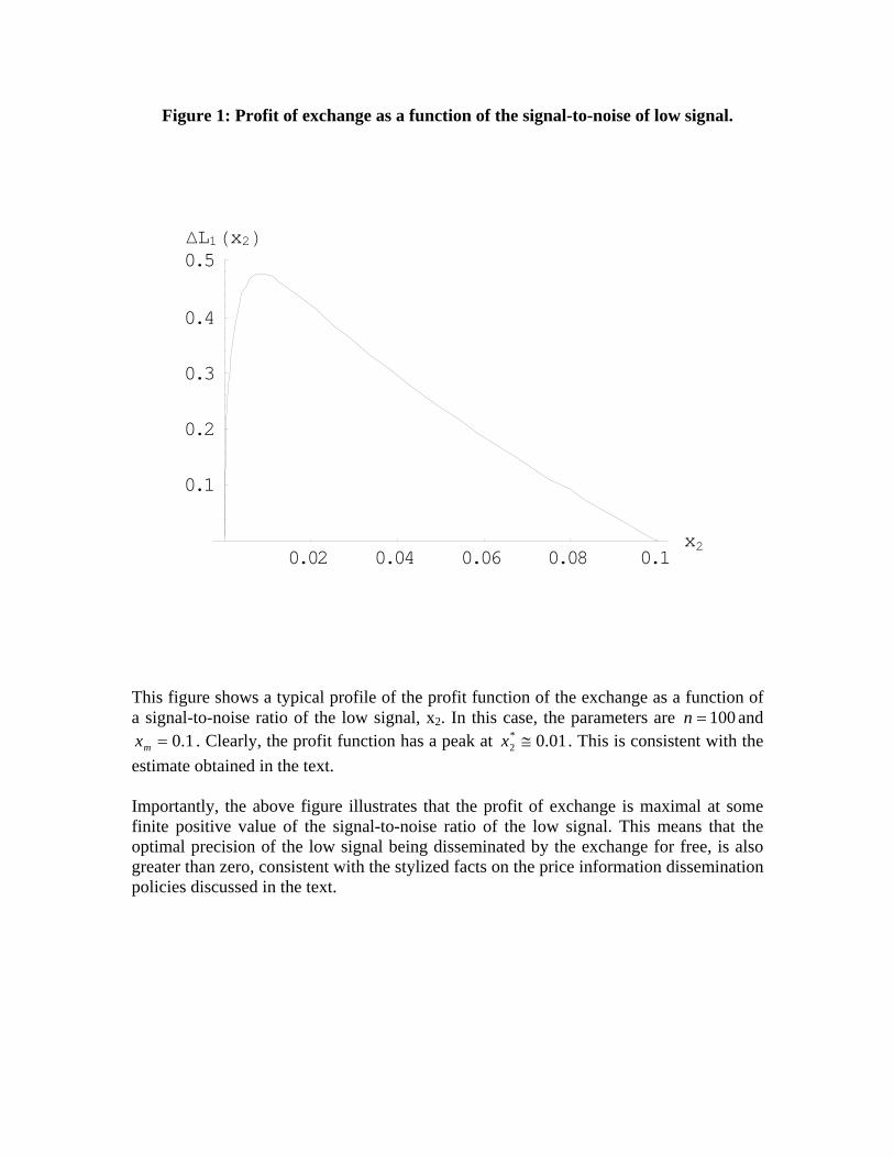
Figure 1: Profit of exchange as a function of the signal-to-noise of low signal.

0.02 0.04 0.06 0.08 0.1x2

0.1

0.2

0.3

0.4

0.5∆L1Hx2L

This figure shows a typical profile of the profit function of the exchange as a function of a signal-to-noise ratio of the low signal, x2. In this case, the parameters are 100=n and

1.0=mx . Clearly, the profit function has a peak at 01.0*2 ≅x . This is consistent with the

estimate obtained in the text. Importantly, the above figure illustrates that the profit of exchange is maximal at some finite positive value of the signal-to-noise ratio of the low signal. This means that the optimal precision of the low signal being disseminated by the exchange for free, is also greater than zero, consistent with the stylized facts on the price information dissemination policies discussed in the text.

Figure 2: Exchange objective as a function of the compensation parameter and the number of high type agents

0 100 200 300 400 500 600n1

0

0.2

0.4

0.6

0.8

1

q

Two-dimensional contour plot of the exchange objective function as a function of the compensation parameter q ∈ [0, 1] and the number of high type agents n₁. The total number of informed agents is n=1000 and the high price signal has a precision of 101, =pµ . As is clear from Fig.2, the critical value in this case is 6.0≅cq .

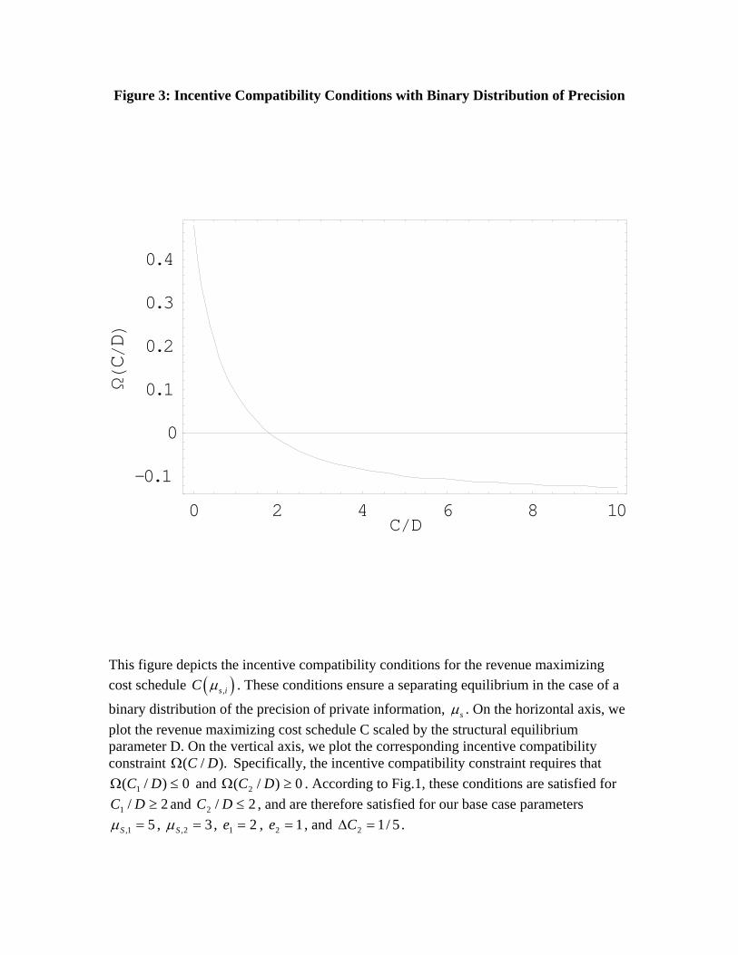
Figure 3: Incentive Compatibility Conditions with Binary Distribution of Precision

0 2 4 6 8 10CêD

-0.1

0

0.1

0.2

0.3

0.4

ΩHCêDL

This figure depicts the incentive compatibility conditions for the revenue maximizing cost schedule ( ),s iC µ . These conditions ensure a separating equilibrium in the case of a

binary distribution of the precision of private information, sµ . On the horizontal axis, we plot the revenue maximizing cost schedule C scaled by the structural equilibrium parameter D. On the vertical axis, we plot the corresponding incentive compatibility constraint )./( DCΩ Specifically, the incentive compatibility constraint requires that

0)/( 1 ≤Ω DC and 0)/( 2 ≥Ω DC . According to Fig.1, these conditions are satisfied for 2/1 ≥DC and 2/2 ≤DC , and are therefore satisfied for our base case parameters

51, =Sµ , 32, =Sµ , 21 =e , 12 =e , and 5/12 =∆C .

Figure 4: Revenue Maximizing Cost Schedule with Binary Distribution of Precision

0 0.5 1 1.5 2∆C1ê∆C2

0

0.25

0.5

0.75

1

1.25

1.5

1.75

Hµ1pêµ

2pL2

We characterize the revenue maximizing cost schedule ( ),i p iC µ∆ - shown on the

horizontal axis as a fraction – as a function on the precision of private information, pµ . This plot is properly scaled to suit the binary distribution of agents’ precision of private information. In other words, for a given ratio 21 / CC ∆∆ between cost of obtaining more precise price information as opposed to less precise, there is a corresponding ratio of precisions of private information 2,1, / PP µµ .

Note that ( ),i p iC µ∆ is monotonically increasing in ,p iµ , and can be approximated by a

linear function in the range of ,p iµ that belongs to our base case set of parameters and

satisfies the incentive compatibility condition. Thus our choice of plotting .)/( 22,1, PP µµ

As before, our parameters are 51, =Sµ , 32, =Sµ , 21 =e , 12 =e , and 5/12 =∆C .

Figure 5: Marginal Value of Price Information as a Function of Private Information

0 2 4 6 8 100

0.2

0.4

0.6

0.8

1

This figure shows the marginal value of information, ( ),p sµ µΦ , as a function of the

price precision pµ , for two precisions of private signal sµ . The lower and upper curves correspond to parameter values of 0.5sµ = and 5sµ = , respectively. Clearly, the marginal

value ( ),p sµ µΦ increases in the precision of the private signal, reflecting the fact that the two kinds of signals are complementary in our model. Furthermore, note that

( )0 , 1p sµ µ≤ Φ ≤ for any positive precisions, and therefore the conditions for

equilibrium derived in the text can only be satisfied within the parameter range [ ]0,1ε ∈ .

Figure 6: Equilibrium price precision as a function of private precision

0 10 20 30 40 50ms

0

1

2

3

4

m p

This figure depicts the equilibrium precision of acquired pricing information, ( )p sµ µ , as a function of the precision of private information sµ . This is done for several values of

the cost schedule parameter 2BD

ε = . The upper curve corresponds to 0.8ε = , the

middle curve to 0.5ε = , and the lower curve to 0.3ε = . Note that as the cost parameter increases, the maximal acquired price precision goes down.

Figure 7: Equilibrium probability density of price precision

0.65 0.7 0.75 0.8 0.85 0.9 0.95µp

0.5

1

1.5

2

2.5

3

ρHµ

pL

This figure plots the equilibrium probability density of the distribution of price precision in the case when the precision of private signals is uniformly distributed across the

informed agents. Here, the cost schedule parameter is given by 2 0.5BD

ε = = and the

distribution of the precisions of the private signals is uniform with max 10µ = . As one can see, the distribution is right-skewed in comparison to the uniform distribution of private information. The reason is that the agents with higher precisions of their private signals also tend to acquire more precise information on price. For this reason, the p.d.f. increases for the large price precisions.

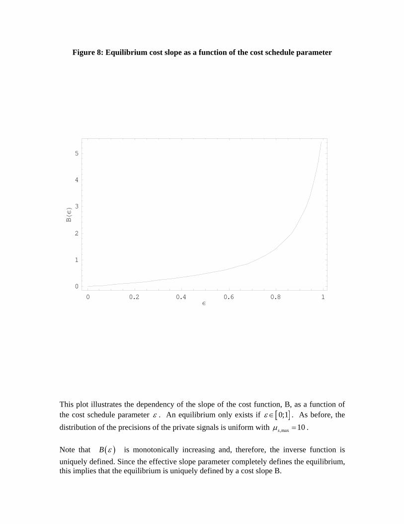
Figure 8: Equilibrium cost slope as a function of the cost schedule parameter

0 0.2 0.4 0.6 0.8 1ε

0

1

2

3

4

5

BHεL

This plot illustrates the dependency of the slope of the cost function, B, as a function of the cost schedule parameter ε . An equilibrium only exists if [ ]0;1ε ∈ . As before, the distribution of the precisions of the private signals is uniform with ,max 10sµ = . Note that ( )B ε is monotonically increasing and, therefore, the inverse function is uniquely defined. Since the effective slope parameter completely defines the equilibrium, this implies that the equilibrium is uniquely defined by a cost slope B.

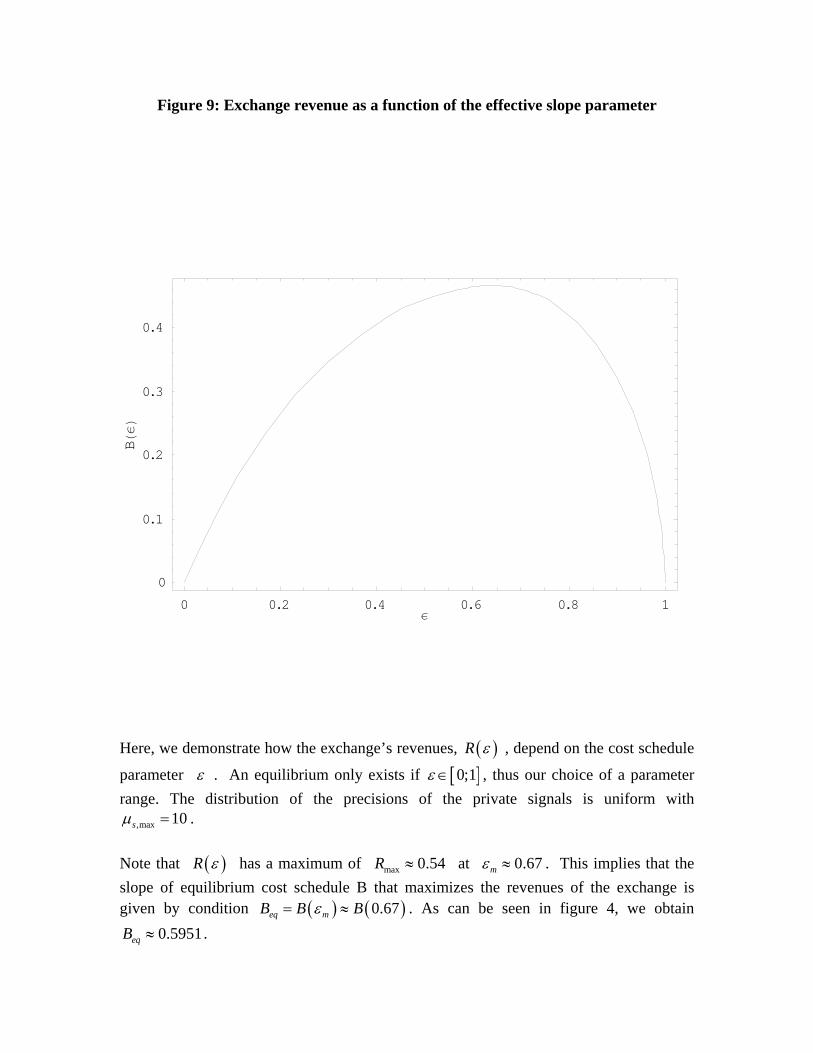
Figure 9: Exchange revenue as a function of the effective slope parameter

0 0.2 0.4 0.6 0.8 1ε

0

0.1

0.2

0.3

0.4

BHεL

Here, we demonstrate how the exchange’s revenues, ( )R ε , depend on the cost schedule

parameter ε . An equilibrium only exists if [ ]0;1ε ∈ , thus our choice of a parameter range. The distribution of the precisions of the private signals is uniform with

,max 10sµ = . Note that ( )R ε has a maximum of max 0.54R ≈ at 0.67mε ≈ . This implies that the slope of equilibrium cost schedule B that maximizes the revenues of the exchange is given by condition ( ) ( )0.67eq mB B Bε= ≈ . As can be seen in figure 4, we obtain

0.5951eqB ≈ .

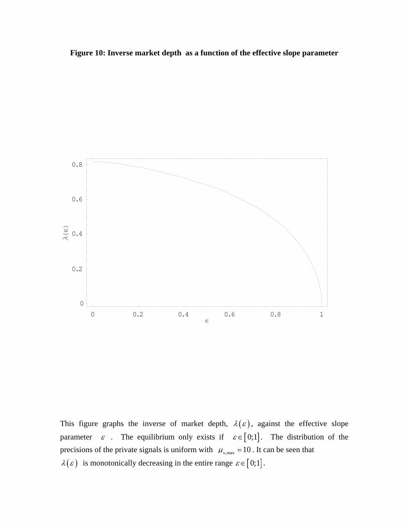
Figure 10: Inverse market depth as a function of the effective slope parameter

0 0.2 0.4 0.6 0.8 1ε

0

0.2

0.4

0.6

0.8

λHεL

This figure graphs the inverse of market depth, ( )λ ε , against the effective slope

parameter ε . The equilibrium only exists if [ ]0;1ε ∈ . The distribution of the precisions of the private signals is uniform with ,max 10sµ = . It can be seen that

( )λ ε is monotonically decreasing in the entire range [ ]0;1ε ∈ .

Figure 11: Exchange objective as a function of the effective slope parameter

0 0.2 0.4 0.6 0.8 1ε

-0.1

0

0.1

0.2

0.3

RHεL−

1 5λHεL

The previous plot, figure 8, showed exchange revenue ignoring the impact that sale of pricing data has on market liquidity. By contrast, here we illustrate how the exchanges true objective function, ( ) ( ) ( )L R qε ε λ ε= − , varies with the cost schedule parameterε . The term )(ελq is the expected compensation the exchange needs to provide to uninformed traders – we can refer to it as the exchanges shadow cost of illiquidity. In this case, the weight is q = 0.2. The equilibrium only exists if [ ]0;1ε ∈ . The distribution of the precisions of the private signals is uniform with ,max 10sµ = . Note that ( )L ε has a maximum of max 0.41L ≈ at 0.75Lε ≈ . This implies that the

slope of equilibrium cost schedule B that maximizes ( )L ε is given by condition

( ) ( )0.75L LB B Bε= ≈ . As can be seen in figure 4, this corresponds to a value of 0.77LB ≈ .

Figure 12: Revenue maximizing slope of the cost schedule as a function of the maximum precision of the private information

2.5 5 7.5 10 12.5 15 17.5 20µs,m

0.6

0.8

1

1.2

1.4

1.6

1.8

B RHµ

s,mL

Here, we show how the exchange’s revenue maximizing slope of the cost schedule,

( ),R s mB µ , depends on the maximum precision of the private information ,s mµ .

Note that ( ),R s mB µ monotonically decreases in ,s mµ , implying that the indirect effect on the agents’ strategies due to the collective contribution of all other agents, prevails in the range of parameters under consideration.