price/earnings investing - j.p. morgan · price/earnings investing ... equity holdings when the...

Price/earnings investingOne picture requires a thousand words

Reality In Returns series | Issue 1, November 2011

FOR INSTITUTIONAL AND PROFESSIONAL INVESTOR USE ONLY | NOT FOR RETAIL USE OR PUBLIC DISTRIBUTION

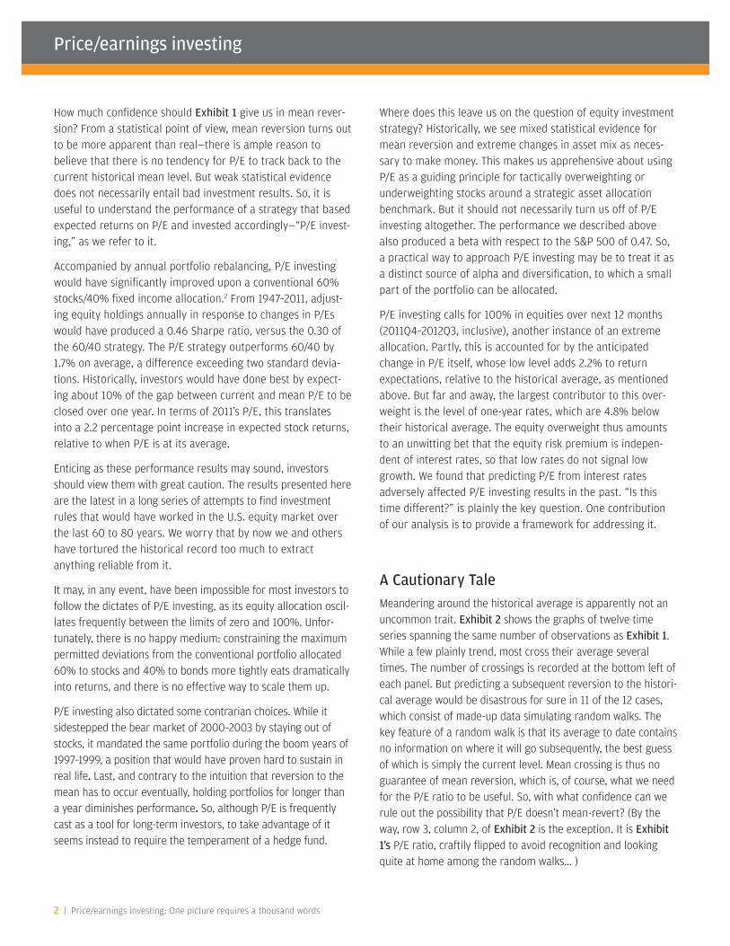
EXHIBIT 1: THE PICTURE... S&P 500 PRICE/EARNINGS RATIO

0

5

10

15

Rat

io

20

25

30

1950 1960 1970 1980 1990 2000 2010

Source: J.P. Morgan Asset Management calculations based on data described in Appendix II.

A picture of the market’s price/earnings ratio (P/E) is seemingly a fixture in commentary on the equity market. Invariably, the P/E history is accompanied by a horizontal line indicating its historical average, which is currently 15, implying that the cost of $1 of earnings has averaged $15 since 1927.

Long-term investors are often counseled to increase their equity holdings when the market’s P/E is below its historical average, as it is now, on the presumption that stock prices will eventually increase to restore P/E to the average.1 Because the speed of reversion is uncertain, investing on the basis of P/E is typically framed as a buy-and-hold strategy, rather than as a trading rule.

We question the implicit faith in mean reversion of P/E lurking behind this advice and find little to justify P/E investing as a principle of long-horizon asset allocation. As an independent source of alpha, however, it has legs.

IN BRIEF• Market commentary often recommends buying stocks when

P/E has fallen below its historical average, a recommendation that implicitly assumes that P/E reverts to a mean.

• We put this implicit assumption to a rigorous test, measuring its validity against annual market returns from 1947 to 2011.

• The statistical case that the market’s P/E actually mean-reverts is weak. Reverting to a long-term mean involves something more substantial than crossing the historical average, which is unavoidable by definition.

• On the other hand, annual portfolio decisions based on P/E mean reversion would have performed well, with a Sharpe ratio between 1947 and 2011 of 0.46, versus 0.30 for a conventional 60/40 strategy.

• We would not recommend P/E as a long-term asset allocation principle. The evidence is too mixed and to succeed P/E investing requires large equity allocation changes, while holding positions longer than one year undermines performance.

• Nevertheless, the evidence is strong enough to recommend P/E investing as a separate source of alpha and diversification.

Price/earnings investing

2 | Price/earnings investing: One picture requires a thousand words

How much confidence should Exhibit 1 give us in mean rever-sion? From a statistical point of view, mean reversion turns out to be more apparent than real—there is ample reason to believe that there is no tendency for P/E to track back to the current historical mean level. But weak statistical evidence does not necessarily entail bad investment results. So, it is useful to understand the performance of a strategy that based expected returns on P/E and invested accordingly—“P/E invest-ing,” as we refer to it.

Accompanied by annual portfolio rebalancing, P/E investing would have significantly improved upon a conventional 60% stocks/40% fixed income allocation.2 From 1947–2011, adjust-ing equity holdings annually in response to changes in P/Es would have produced a 0.46 Sharpe ratio, versus the 0.30 of the 60/40 strategy. The P/E strategy outperforms 60/40 by 1.7% on average, a difference exceeding two standard devia-tions. Historically, investors would have done best by expect-ing about 10% of the gap between current and mean P/E to be closed over one year. In terms of 2011’s P/E, this translates into a 2.2 percentage point increase in expected stock returns, relative to when P/E is at its average.

Enticing as these performance results may sound, investors should view them with great caution. The results presented here are the latest in a long series of attempts to find investment rules that would have worked in the U.S. equity market over the last 60 to 80 years. We worry that by now we and others have tortured the historical record too much to extract anything reliable from it.

It may, in any event, have been impossible for most investors to follow the dictates of P/E investing, as its equity allocation oscil-lates frequently between the limits of zero and 100%. Unfor-tunately, there is no happy medium: constraining the maximum permitted deviations from the conventional portfolio allocated 60% to stocks and 40% to bonds more tightly eats dramatically into returns, and there is no effective way to scale them up.

P/E investing also dictated some contrarian choices. While it sidestepped the bear market of 2000–2003 by staying out of stocks, it mandated the same portfolio during the boom years of 1997–1999, a position that would have proven hard to sustain in real life. Last, and contrary to the intuition that reversion to the mean has to occur eventually, holding portfolios for longer than a year diminishes performance. So, although P/E is frequently cast as a tool for long-term investors, to take advantage of it seems instead to require the temperament of a hedge fund.

Where does this leave us on the question of equity investment strategy? Historically, we see mixed statistical evidence for mean reversion and extreme changes in asset mix as neces-sary to make money. This makes us apprehensive about using P/E as a guiding principle for tactically overweighting or underweighting stocks around a strategic asset allocation benchmark. But it should not necessarily turn us off of P/E investing altogether. The performance we described above also produced a beta with respect to the S&P 500 of 0.47. So, a practical way to approach P/E investing may be to treat it as a distinct source of alpha and diversification, to which a small part of the portfolio can be allocated.

P/E investing calls for 100% in equities over next 12 months (2011Q4–2012Q3, inclusive), another instance of an extreme allocation. Partly, this is accounted for by the anticipated change in P/E itself, whose low level adds 2.2% to return expectations, relative to the historical average, as mentioned above. But far and away, the largest contributor to this over-weight is the level of one-year rates, which are 4.8% below their historical average. The equity overweight thus amounts to an unwitting bet that the equity risk premium is indepen-dent of interest rates, so that low rates do not signal low growth. We found that predicting P/E from interest rates adversely affected P/E investing results in the past. “Is this time different?” is plainly the key question. One contribution of our analysis is to provide a framework for addressing it.

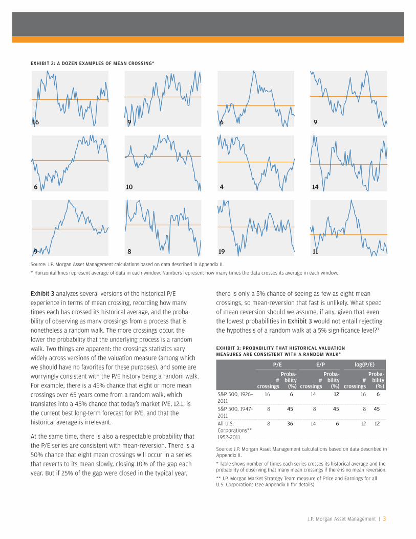
A Cautionary TaleMeandering around the historical average is apparently not an uncommon trait. Exhibit 2 shows the graphs of twelve time series spanning the same number of observations as Exhibit 1. While a few plainly trend, most cross their average several times. The number of crossings is recorded at the bottom left of each panel. But predicting a subsequent reversion to the histori-cal average would be disastrous for sure in 11 of the 12 cases, which consist of made-up data simulating random walks. The key feature of a random walk is that its average to date contains no information on where it will go subsequently, the best guess of which is simply the current level. Mean crossing is thus no guarantee of mean reversion, which is, of course, what we need for the P/E ratio to be useful. So, with what confidence can we rule out the possibility that P/E doesn’t mean-revert? (By the way, row 3, column 2, of Exhibit 2 is the exception. It is Exhibit 1’s P/E ratio, craftily flipped to avoid recognition and looking quite at home among the random walks… )

J.P. Morgan Asset Management | 3

Exhibit 3 analyzes several versions of the historical P/E experience in terms of mean crossing, recording how many times each has crossed its historical average, and the proba-bility of observing as many crossings from a process that is nonetheless a random walk. The more crossings occur, the lower the probability that the underlying process is a random walk. Two things are apparent: the crossings statistics vary widely across versions of the valuation measure (among which we should have no favorites for these purposes), and some are worryingly consistent with the P/E history being a random walk. For example, there is a 45% chance that eight or more mean crossings over 65 years come from a random walk, which translates into a 45% chance that today’s market P/E, 12.1, is the current best long-term forecast for P/E, and that the historical average is irrelevant.

At the same time, there is also a respectable probability that the P/E series are consistent with mean-reversion. There is a 50% chance that eight mean crossings will occur in a series that reverts to its mean slowly, closing 10% of the gap each year. But if 25% of the gap were closed in the typical year,

EXHIBIT 2: A DOZEN EXAMPLES OF MEAN CROSSING*


* Horizontal lines represent average of data in each window. Numbers represent how many times the data crosses its average in each window.

16 9 6 9

6 10 4 14

9 8 19 11

EXHIBIT 3: PROBABILITY THAT HISTORICAL VALUATION MEASURES ARE CONSISTENT WITH A RANDOM WALK*

P/E E/P log(P/E)

# crossings

Proba-bility

(%)#

crossings

Proba-bility

(%)#

crossings

Proba- bility

(%)S&P 500, 1926–2011

16 6 14 12 16 6

S&P 500, 1947–2011

8 45 8 45 8 45

All U.S. Corporations** 1952–2011

8 36 14 6 12 12


* Table shows number of times each series crosses its historical average and the probability of observing that many mean crossings if there is no mean reversion.

** J.P. Morgan Market Strategy Team measure of Price and Earnings for all U.S. Corporations (see Appendix II for details).

there is only a 5% chance of seeing as few as eight mean crossings, so mean-reversion that fast is unlikely. What speed of mean reversion should we assume, if any, given that even the lowest probabilities in Exhibit 3 would not entail rejecting the hypothesis of a random walk at a 5% significance level?3



What Are Valuation Ratios Worth?Statistical analysis provides a tightly controlled picture of what drives the numbers under study, but significance is not neces-sarily the right yardstick for investment decisions. For this pur-pose, it is more useful to cut to the chase and assess directly whether P/E investing would have improved the returns of an investor who was willing to assume P/E reverted to the mean. We therefore calculate the performance of an investment rule that determines its equity/fixed income mix every year based on expected mean reversion of P/E.4 Specifically, each year the relationship between P/E and equity returns is calculated from the historical experience accumulated to that date. From this, a forecast of equity returns over the next year is made (see Appendix I), and an allocation is made between the S&P 500 index (or its predecessors) and one-year Treasuries5 to match the expected return volatility of a 60/40 stocks/Treasuries portfolio. To rule out leverage and short selling, we limit the actual equity allocation to the zero-to-100% range. A year passes, the portfolio incurs a return, and the whole process is repeated, with the latest year’s returns included in the re-estimation of expected returns and risks.6

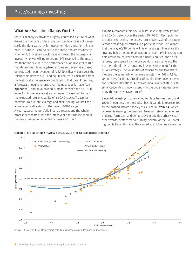
Exhibit 4 compares this one-year P/E investing strategy and the 60/40 strategy over the period 1947–2011. Each point in the chart represents the excess return over cash of a strategy versus excess equity returns in a particular year. This means that the gray 60/40 points will lie on a straight line since the strategy holds the equity allocation constant. P/E investing can hold anywhere between zero and 100% equities, and so its returns, represented by the orange dots, are scattered. The Sharpe ratio of the P/E strategy is 0.46, versus 0.30 for the 60/40 strategy. The volatilities of returns for the two strate-gies are the same, while the average return of P/E is 4.8%, versus 3.1% for the 60/40 allocation. The difference exceeds two standard deviations. At conventional levels of statistical significance, this is inconsistent with the two strategies deliv-ering the same average return.7

Since P/E investing is constrained to place between zero and 100% in equities, the theoretical best it can do is represented by the dashed, brown “hockey-stick” line in Exhibit 4, which represents earning the one-year Treasury rate when equities underperform cash and being 100% in equities otherwise… in other words, perfect market timing. Several of the P/E invest-ing points lie on this line. The curved solid blue line shows the


0.4

0.3

0.2

0.1

0.0

0.1

0.2

0.3

0.4

-0.6 -0.4 -0.2 0.0 0.2 0.4 0.6

Stra

tegy

exc

ess

retu

rn

Equity excess return

60/40 equity/fixed income strategy

P/E investing

S&P 500 call option

Perfect market timing

Best fit of P/E investing

EXHIBIT 4: P/E INVESTING STRATEGY VERSUS 60/40 STOCK/FIXED INCOME STRATEGY


regression fit of P/E investing returns by a quadratic function of the equity return. Including a quadratic term in this regres-sion makes it possible to differentiate P/E investing from sim-ple leverage, in which case the return would just be a straight linear function of the equity return (like the 60/40 strategy), and the quadratic term in the regression would be zero. As it turns out, the quadratic term is quite large, and five standard deviations away from zero, so it appears that a strategy of buying stocks when their P/Es have fallen below their long-term averages involves an element of market timing. The R2 of this regression is significantly higher that the R2 of a linear equation: 0.75, compared to 0.63.

Exhibit 4 also shows the excess return of investing in a hypo-thetical one-year call option on the S&P 500, with a payoff equal to the perfect market timing line.8 The excess return profile for this strategy is shown by the green dashed line. To the extent that the blue curve lies above this one, it could be argued that P/E investing outperforms the cheapest form of passive market timing, that is, buying a call on the S&P 500. In practice, the option is likely to be more expensive than the theoretical Black-Scholes price we have used, and the achiev-able passive return would lie below the green line.

Through the lens of investment results, how do the mean reversion and random walk perspectives of P/E compare? A strategy using the random walk view would ignore the estimated degree of mean reversion at any point, and forecast P/E as the most recent level, plus the historical average change in P/E. The resulting Sharpe ratio is 0.39, quite a bit lower than P/E investing’s 0.46, and the average return is 0.7% less. Neither gap is bigger than one standard deviation, however, so the difference is not statistically significant. Thus, while the purely statistical evidence offers a lot of support for the random

walk view over mean reversion; as we said, it uses a very particular yardstick. When we measure in terms more relevant to investment performance, mean reversion seems to have an edge, although not one that is very precisely measured.

P/E’s ChallengesExhibit 5 shows how P/E investing’s equity weight moved over time. Apparently, to attain the returns documented in Exhibit 4, the P/E strategy had to undergo extreme year-over-year rebal-ancing. We found that constraining these swings to narrower bands materially worsened the performance of P/E investing. Sometimes, as in the 1970s and the most recent decade, P/E investing corresponded to quite accurate market timing, as evi-denced in Exhibits 6A and 6B, which break down returns and Sharpe ratios by decade. At other times these switches required P/E investing to occupy a very lonely position. In particular, it

EXHIBIT 5: HOW P/E INVESTING’S EQUITY WEIGHT MOVED OVER TIME*


* Solid blue line represents equity weights of P/E investing, constrained to be between zero and 100%. Dashed blue line is unconstrained.

-1.0

-0.5

0.0

0.5

1.0

1.5

2.0

2.5

1950 1960 1970 1980 1990 2000 2010

Stra

tegy

equ

ity

wei

ght

P/E investing60/40 equity/cash

EXHIBIT 6A: AVERAGE EXCESS RETURN FOR 60/40 AND P/E STRATEGIES EXHIBIT 6B: SHARPE RATIOS FOR 60/40 AND P/E STRATEGIES


Perc

ent

Shar

pe r

atio

P/E investing 60/40 P/E investing 60/40

-4

-2

0

2

4

6

8

10

12

14

1947–59 1960s 1970s 1980s 1990s 2000–11-0.4

-0.2

0.0

0.2

0.4

0.6

0.8

1.0

1.2

1.4

1.6

1947–59 1960s 1970s 1980s 1990s 2000–11



placed a zero weight on equities in the late 1990s, when equity returns were quite high, and the 60/40 strategy outperformed. We imagine that it would have been difficult for P/E investing to hold down a steady job during this period. Its revenge came in the early years of the last decade, when it continued to under-weight equities through the end of the dot-com boom.9

All the performance results discussed so far reflect an invest-ment horizon of just one year. As we mentioned at the outset, P/E investing is usually positioned as a long-term strategy. We interpret this to mean that an investor would do better buying and holding equities for several years when P/Es are low rath-er than rebalancing every year. This is a proposition we can test. To implement a buy and hold strategy with, say, a three-year horizon, we divide the portfolio into three initially equal portfolios, each of which we rebalance in a different year in the cycle.

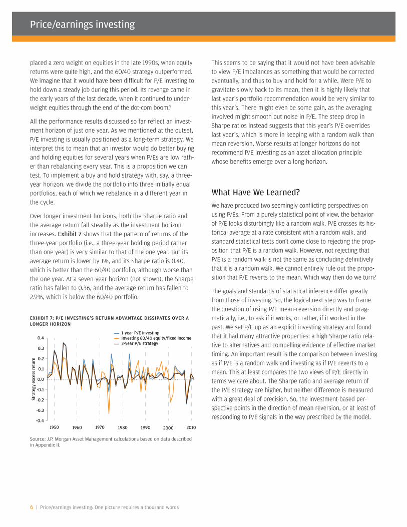
Over longer investment horizons, both the Sharpe ratio and the average return fall steadily as the investment horizon increases. Exhibit 7 shows that the pattern of returns of the three-year portfolio (i.e., a three-year holding period rather than one year) is very similar to that of the one year. But its average return is lower by 1%, and its Sharpe ratio is 0.40, which is better than the 60/40 portfolio, although worse than the one year. At a seven-year horizon (not shown), the Sharpe ratio has fallen to 0.36, and the average return has fallen to 2.9%, which is below the 60/40 portfolio.

This seems to be saying that it would not have been advisable to view P/E imbalances as something that would be corrected eventually, and thus to buy and hold for a while. Were P/E to gravitate slowly back to its mean, then it is highly likely that last year’s portfolio recommendation would be very similar to this year’s. There might even be some gain, as the averaging involved might smooth out noise in P/E. The steep drop in Sharpe ratios instead suggests that this year’s P/E overrides last year’s, which is more in keeping with a random walk than mean reversion. Worse results at longer horizons do not recommend P/E investing as an asset allocation principle whose benefits emerge over a long horizon.

What Have We Learned?We have produced two seemingly conflicting perspectives on using P/Es. From a purely statistical point of view, the behavior of P/E looks disturbingly like a random walk. P/E crosses its his-torical average at a rate consistent with a random walk, and standard statistical tests don’t come close to rejecting the prop-osition that P/E is a random walk. However, not rejecting that P/E is a random walk is not the same as concluding definitively that it is a random walk. We cannot entirely rule out the propo-sition that P/E reverts to the mean. Which way then do we turn?

The goals and standards of statistical inference differ greatly from those of investing. So, the logical next step was to frame the question of using P/E mean-reversion directly and prag-matically, i.e., to ask if it works, or rather, if it worked in the past. We set P/E up as an explicit investing strategy and found that it had many attractive properties: a high Sharpe ratio rela-tive to alternatives and compelling evidence of effective market timing. An important result is the comparison between investing as if P/E is a random walk and investing as if P/E reverts to a mean. This at least compares the two views of P/E directly in terms we care about. The Sharpe ratio and average return of the P/E strategy are higher, but neither difference is measured with a great deal of precision. So, the investment-based per-spective points in the direction of mean reversion, or at least of responding to P/E signals in the way prescribed by the model.

EXHIBIT 7: P/E INVESTING’S RETURN ADVANTAGE DISSIPATES OVER A LONGER HORIZON


-0.4

-0.3

-0.2

-0.1

0.0

0.1

0.2

0.3

0.4

1950 1960 1970 1980 1990 2000 2010

Stra

tegy

exc

ess

retu

rn

1-year P/E investingInvesting 60/40 equity/fixed income3-year P/E strategy


Occupational HazardsWe cannot weigh our choices sensibly without addressing the problem of “data snooping,” which describes practices, unwit-ting or otherwise, that make results like ours less reliable than they seem at first glance. They are unavoidable and potentially lethal occupational hazards of dealing with financial markets data. They all imply that P/E investing will perform less well in the future than in the past.

First, the models we are using are the result of a long tradition of trying to explain equity returns. The same return data have been picked over by legions of highly motivated investigators, whose incentives are skewed toward finding positive results. The academic articles on which our analysis builds collectively examined a couple of dozen stock return predictors. These in turn had each been advanced separately by other investiga-tors. One can only imagine the heaps of others that lie on the collective cutting-room floor. This is not to say that following P/E is wrong, just that, if there is an accidental correlation in the data, chances are, we would have found it.

Second, it is often implied that the out-of-sample forecasting method we have used to evaluate investment rules is not vul-nerable to the gaming that is so easy with a within-sample fit. We are not convinced. For concreteness, imagine splitting the 1947–2011 data into two sub-periods, A and B. It is certainly true that there are more regression models that fit equity returns within sub-period A well than there are that also, without alteration, produce a high Sharpe ratio out of sample during sub-period B. But the implicit suggestion here, that out-of-sample forecasting only gets to try its luck on B once, is inac-curate. Effectively, an iteration takes place along these lines:

(1) fit a model to A, calculate its Sharpe ratio over B

(2) if the Sharpe ratio is high enough, stop and declare victory, otherwise, repeat (1) with a new model

For any given model within this recipe, the Sharpe ratio calcu-lation on sub-period B is out of sample. But the entire recipe (Steps 1 and 2) gets a look at B before deciding on which model to back. So, for the recipe, B does not seem materially less out of sample than A.

To breathe some life into this abstraction, we offer some exam-ples of models that seemed like a good idea at the time but were discarded in favor of the P/E investing rule we have described. One is that we break down equity returns into three components (P/E growth, earnings growth and dividends) and forecast each separately, before combining them into a forecast. This works better than pooling the components into one model to predict equity returns directly.10 Presumably, we would have used the direct approach had that worked better and not missed a beat. We, and other investigators, also tried many models incorporat-ing interest rates, real and nominal, in the spirit of the so-called “Fed model,” and the notion that the equity risk premium drives equity returns. None of these performed as well as the P/E rule, and consequently we passed on them. Anyone who contemplates putting money to work in P/E investing needs to be comfortable with the process that shortlisted it.

So, how should investors regard P/E investing? In its favor, there is the high Sharpe ratio, although the occupational hazard of data snooping is a caution. Against, we have the statistical verdict on mean reversion, which ranges from weak support to outright rejection. Similarly, P/E investing seems to require exceptionally wide and frequent swings in asset allocation and does not work as a long-term buy-and-hold strategy. It does not seem to make the grade as a principle investors should use for long-horizon asset allocation between equities and fixed income, which is the context in which it is usually offered up.

Yet it is hard to let go of the performance results, which seem as compelling as any typical alpha-generating strategy. To the high Sharpe ratio and average return, we can add that P/E investing turned in a relatively low beta of 0.47 over the 1947–2011 period. Long/short equity hedge funds have a beta of 0.46 to the S&P 500.11 Maybe this is where P/E investing belongs: as one source of alpha among many across which a portfolio is diversified. The investor need not have great faith in any one of these; just an expectation that each has some positive chance of outperforming. As long as their correlation is low, diversification will make up for lack of conviction. In this context, the practical drawbacks mentioned above are not important. It doesn’t matter if only a few percentage points of the portfolio are allocated to a strategy that needs to rebal-ance frequently and by a lot. For this reason, it may suit inves-tors better to think of P/E investing more as a separate source of alpha than a guiding principle of asset allocation.



2012 and the Way ForwardP/E investing’s current allocation is 100% equities, which is the consequence of a forecast of excess returns for equities of 12% over the next 12 months. Exhibit 8 shows the sources of this forecast.

While mean reversion of P/E and earnings growth forecasts exceed their historical averages, far and away the single biggest contributor to the 12% excess return forecast for stocks is the risk-free interest rate. Allowing P/E and earnings growth fore-casts to depend on interest rates, real and/or nominal, short or long, failed miserably when back-tested in terms of the Sharpe ratio criterion (see data snooping, above). Consequently, none of the separate forecasting models for the three components of stock returns listed in the table rely on an interest rate. As a result, the model pays no attention to the breakdown of equity returns between risk-free returns (real or nominal) and the equity risk premium. By default, its forecast therefore assumes that the equity risk premium is not constant but will expand to take up the slack between one-year rates and the forecast return. This may or may not be a drawback of P/E investing, but plainly, something has to give. For 2012, investors have to choose between the equity risk premium being an outlier, or P/E investing giving the wrong signal.

Appendix I: Forecasting components of equity returns

We derive the relationship between equity returns and P/E ratios as follows:12

From this last equation, we take the logarithm of both sides and arrive at the following identity:

total return on equity = Dp + De + δ

which says that the logarithm of the total return from equity including dividends is composed of the log change in P/E ratio (Dp), the log change in earnings (De) and δ, which is the log of the end-of-period dividend-price ratio.

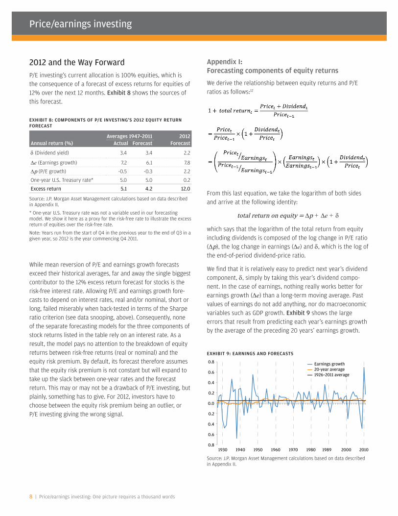
We find that it is relatively easy to predict next year’s dividend component, δ, simply by taking this year’s dividend compo-nent. In the case of earnings, nothing really works better for earnings growth (De) than a long-term moving average. Past values of earnings do not add anything, nor do macroeconomic variables such as GDP growth. Exhibit 9 shows the large errors that result from predicting each year’s earnings growth by the average of the preceding 20 years’ earnings growth.

EXHIBIT 8: COMPONENTS OF P/E INVESTING’S 2012 EQUITY RETURN FORECAST


* One-year U.S. Treasury rate was not a variable used in our forecasting model. We show it here as a proxy for the risk-free rate to illustrate the excess return of equities over the risk-free rate.

Note: Years run from the start of Q4 in the previous year to the end of Q3 in a given year, so 2012 is the year commencing Q4 2011.

Averages 1947–2011 2012Annual return (%) Actual Forecast Forecast

δ (Dividend yield) 3.4 3.4 2.2

De (Earnings growth) 7.2 6.1 7.8

Dp (P/E growth) -0.5 -0.3 2.2

One-year U.S. Treasury rate* 5.0 5.0 0.2

Excess return 5.1 4.2 12.0

EXHIBIT 9: EARNINGS AND FORECASTS


0.8

0.6

0.4

0.2

0.0

0.2

0.4

0.6

0.8

1930 1940 1950 1960 1970 1980 1989 2000 2010

Earnings growth20-year average1926–2011 average


The volatility of these forecast errors is about 15% lower than the errors around the 1926–2011 average (which wouldn’t have been accessible to the investment strategy prior to 2011 in any case), suggesting that average earnings growth changes slowly over time; beyond that, De is just highly variable noise and, consequently, very hard to predict.

Forecasting P/E seems to meet with more success. For brevity, we denote the logarithm of the P/E ratio in year t by pt, so its rate of change is Dp ≡ pt+1 – pt. Each year, past yearly changes in P/E are regressed on the level of P/E at the start of the respective year. This is used to predict Dp for the next year, from the current level of P/E. This involves estimating α and β in:

Dp ≡ pt+1 - pt = α - βpt + errort+1

If β is zero, this equation says that is unrelated to anything to do with the level of P/E (pt); it is simply random noise, and P/E is consequently a random walk (with a “drift” if α is not zero). This corresponds to the random walk investment strategy discussed in the text. If β is positive, then P/E reverts to its mean. Earlier, we described mean reversion in terms of the proportion of the gap between the current value and the average that is narrowed in one year. This proportion corresponds to β in this equation, while the mean is α/β.13 This comes out more clearly from an equivalent version of the equation:

Dp ≡ pt+1 - pt = β (α/β - pt ) + errort+1

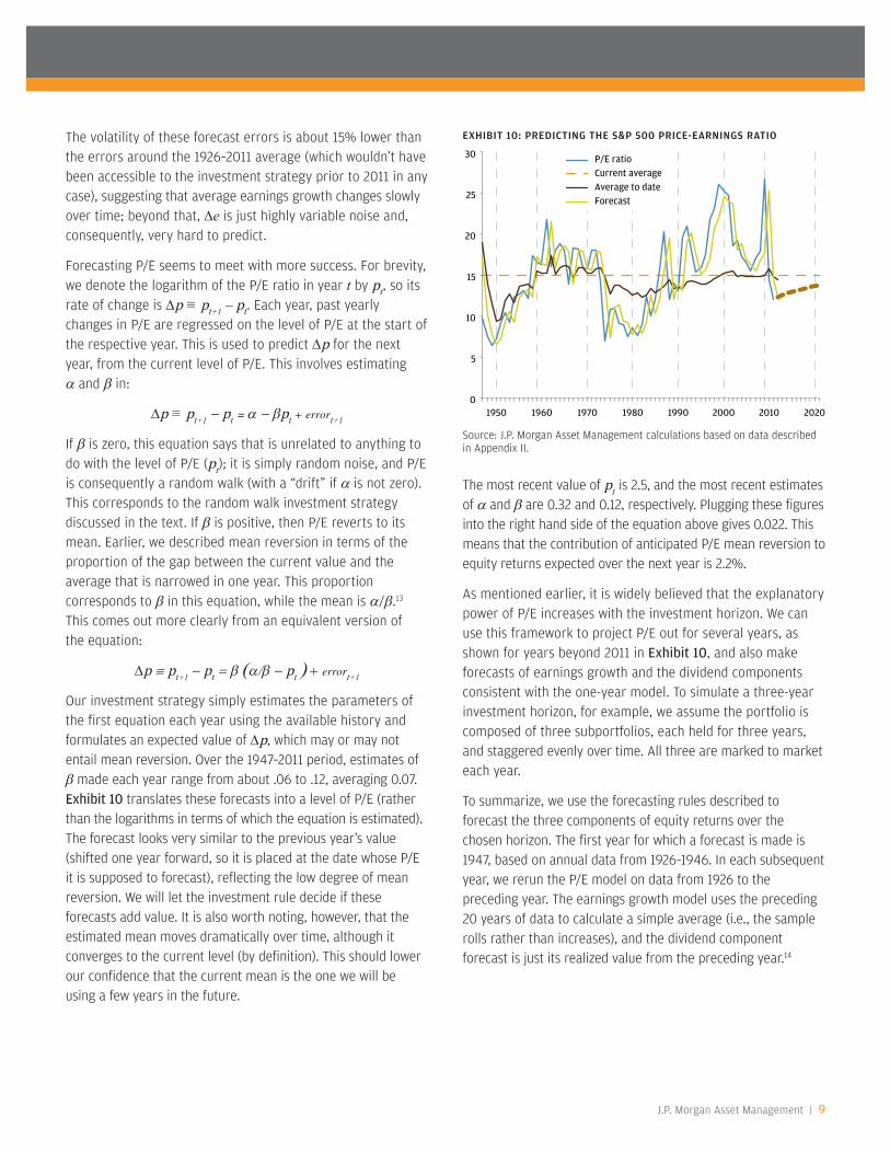
Our investment strategy simply estimates the parameters of the first equation each year using the available history and formulates an expected value of Dp, which may or may not entail mean reversion. Over the 1947–2011 period, estimates of β made each year range from about .06 to .12, averaging 0.07. Exhibit 10 translates these forecasts into a level of P/E (rather than the logarithms in terms of which the equation is estimated). The forecast looks very similar to the previous year’s value (shifted one year forward, so it is placed at the date whose P/E it is supposed to forecast), reflecting the low degree of mean reversion. We will let the investment rule decide if these forecasts add value. It is also worth noting, however, that the estimated mean moves dramatically over time, although it converges to the current level (by definition). This should lower our confidence that the current mean is the one we will be using a few years in the future.

The most recent value of pt is 2.5, and the most recent estimates of α and β are 0.32 and 0.12, respectively. Plugging these figures into the right hand side of the equation above gives 0.022. This means that the contribution of anticipated P/E mean reversion to equity returns expected over the next year is 2.2%.

As mentioned earlier, it is widely believed that the explanatory power of P/E increases with the investment horizon. We can use this framework to project P/E out for several years, as shown for years beyond 2011 in Exhibit 10, and also make forecasts of earnings growth and the dividend components consistent with the one-year model. To simulate a three-year investment horizon, for example, we assume the portfolio is composed of three subportfolios, each held for three years, and staggered evenly over time. All three are marked to market each year.

To summarize, we use the forecasting rules described to forecast the three components of equity returns over the chosen horizon. The first year for which a forecast is made is 1947, based on annual data from 1926–1946. In each subsequent year, we rerun the P/E model on data from 1926 to the preceding year. The earnings growth model uses the preceding 20 years of data to calculate a simple average (i.e., the sample rolls rather than increases), and the dividend component forecast is just its realized value from the preceding year.14

EXHIBIT 10: PREDICTING THE S&P 500 PRICE-EARNINGS RATIO


0

5

10

15

20

25

30

1950 1960 1970 1980 1990 2000 2010 2020

P/E ratioCurrent averageAverage to dateForecast



Appendix II: Description and discussion of data sources

Price: S&P 500 quarter-end values from Goyal and Welch (2008) for 1926–1987 and from S&P 500 Earnings and Estimates Report from Standard & Poor’s website for 1988–2011. Goyal and Welch data is from Center for Research in Security Press (CRSP) for 1927–1987 and from Robert Shiller’s website for 1926.

Earnings: Earnings are 12-month moving sums of earnings on S&P 500 from 1907–2011. We use data back to 1907 rather than 1926 because we use the average of earnings over the preceding 20 years as an input to our forecasts, starting in 1926. The data are from Goyal and Welch 1907–1987 and from S&P 500 Earnings and Estimates Report from Standard & Poor’s website for 1988–2011. Goyal and Welch data is from Robert Shiller’s website. Standard & Poor’s from 1988–2011 are operating earnings, not as reported earnings.

S&P 500 Operating Earnings are available beginning in 1988. Prior to 1988, only S&P 500 As Reported Earnings are avail-able, as per Robert Shiller’s website. We believe that Operating Earnings are the best measure of earnings to use as an input to our forecasting model because Operating Earnings excludes extraordinary items that are not expected to repeat in the future, and thus shouldn’t be considered when predicting future stock prices. Before 1988, we use As Reported Earnings. An alternative to using As Reported Earnings for the periods preceding 1988 would have been to regress Operating Earnings on a similar adjusted earnings data series that goes back further than 1988, such as Adjusted After-Tax Corporate Profits (see below under “Broad-Market Lagged P/E” for details on this data series), and extrapolate the relationship to the pre-1988 period. Although long-term trends of NIPA profits and S&P earnings are broadly similar, we concluded that the post-1988 regression of Operating Earnings on Adjusted After-Tax Corporate Profits was not statistically significant enough to warrant its use, mainly due to short-term differences in the data sets (e.g., dissimilar year-over-year growth rates); conse-quently, we splice together As Reported Earnings data from 1907–1987 with Operating Earnings data from 1988–2011.

Dividends: Dividends are 12-month moving sums of dividends on S&P 500 from 1925–2011. We use data back to 1925 rather than 1926 because we use prior year’s dividends as an input to our div-idend to price ratio forecasts, starting in 1926. The data are from Goyal and Welch 1925–1987 and from S&P 500 Earnings and

Estimates Report from Standard & Poor’s website for 1988–2011. Goyal and Welch data is from Robert Shiller’s website.

Stock returns: S&P 500 quarter-end stock returns are derived from price and dividends data, above. we use end-of-period prices plus 12-month moving sums of dividends less beginning of period prices.

P/E: Trailing price to earnings ratio using end of period prices and end of period 12-month moving sums of earnings.

D/P: Trailing dividend to price ratio using end of period 12-month moving sums of dividends and end of period prices.

Risk-free rate (One-year): One-year rates are beginning of quarter rates from Federal Reserve website for 1953–2011. Beginning of quarter rates are calculated using the average daily rates of the first month in each quarter. Data for 1926–1952 is derived from regression of 1953–2011 Federal Reserve data on annualized 30-day T Bill rate and annualized IT Government rate. Annualized 30-day T bill rates and IT Government rates are from Ibbotson data 1926–2011.

Risk-free rate (Three-year): Three-year rates are beginning of quarter annualized rates from Federal Reserve website for 1953–2011. Beginning of quarter rates are calculated using the average daily rates of the first month in each quarter. Data for 1926–1952 is derived from regression of 1953–2011 Federal Reserve data on annualized 30-day T Bill rate and annualized IT Government rate. Annualized 30-day T bill rates and IT Government rates are from Ibbotson data 1926–2011.

Broad-Market Lagged P/E, i.e., NIPA P/E:

Market value of all U.S. domestic corporationsAdjusted after-tax profits of all U.S. corporations

for the prior four quarters

The Broad-Market Lagged P/E is a measure provided to us by J.P. Morgan Asset Management’s Market Strategy Team. We out-line a brief description below, as well as the pros and cons of this measure as compared to the S&P 500 Price to Earnings ratio.

Price represented by market value of all U.S. domestic corpora-tion, which can be found on line 24 of table L213 in the Federal Reserve’s Z.1 Flow of Funds report. Data are quarterly from 1952–2011. As of the date of this paper, data were only available through the second quarter of 2011. The third quarter value was estimated by running a regression using the value of Wilshire Total Market Index on Flow of Funds Market value measure.


Earnings represented by a trailing four quarter average of adjusted after-tax profits of all U.S. corporations for the 12 months prior to the current quarter. It can be found on line 15 of table 1.12 of the National Income and Product Accounts and available for 1952–2011. Adjusted profits vary from accounting earnings above for a number of reasons, most notably because adjusted after-tax corporate profits are profits from current production only. There are two adjustments: an inventory valu-ation adjustment (IVA) and a capital consumption adjustment (CCAdj). The IVA adjusts inventories to a current-cost basis. The CCAdj adjusts depreciation by valuing assets at current cost and uses consistent depreciation profiles based on used asset prices. The rationale for these two adjustments is that they make after-tax profits closer in concept to S&P 500 earnings.

A note on the advantages and disadvantages of using the NIPA P/E: The NIPA P/E has several important advantages, namely that (1) adjusted after-tax profits are calculated using consistent accounting principles over the entire period; (2) profits are from current production only, excluding capital gains and losses; (3) the data comes from federal tax returns, thus it is arguably more difficult to manipulate than financial accounting data. For our purposes, however, the measure has one significant disadvantage, namely that it includes chapter S and chapter C corporations and, therefore, does not represent an investable universe. We felt that although the NIPA P/E has some advantages over the S&P 500 P/E, using a non-investable universe would be problematic in this context; as a valuation indicator for the institutional investor with an allocation to U.S. equities, the P/E ratio of the S&P 500 is a better option.

BibliographyCampbell, John Y., and Robert J. Shiller, “Valuation Ratios and the Long-Run Stock Market Outlook,” Journal of Portfolio Management 11–26, Winter 1998.

Campbell, John Y., and Robert J. Shiller, “Valuation Ratios and the Long-Run Stock Market Outlook: An Update.” Unpublished paper, Yale University, revised March 2001.

Campbell, John Y., and Robert J. Shiller, “Stock Prices, Earnings, and Expected Dividends,” Journal of Finance, 43(3): 661–676, July 1998(b).

Ferreira, Miguel A., and Pedro Santa-Clara, “Forecasting Stock Market Returns: The Sum of the Parts is More Than the Whole.” National Bureau of Economic Research, 2008.

Hodge, Andrew W., “Comparing NIPA Profits with S&P 500 Profits,” BEA Briefing 22–26, March 2011.

Ibbotson, Roger G., and Peng Chen, “Long-Run Stock Returns: Participating in the Real Economy,” AIMR 88–98, January/February 2003.

Welch, Ivo, and Amit Goyal, “A Comprehensive Look at the Empirical Performance of Equity Premium Prediction,” A Review of Financial Studies, 21(4): 1455–1508, 2008.

Ibbotson, Roger. Ibbotson SBBI Data Series. As of May 31, 2011. Used data from 1926–2011. Morningstar Direct. Morningstar website: http://corporate.morningstar.com/ib/asp/subject.aspx?xmlfile=1225.xml

Shiller, Robert. An Update of Data shown in Chapter 26 of Market Volatility, R. Shiller, MIT Press, 1989, and Irrational Exuberance, Princeton 2005. As of September 30, 2011. Used data from 1926–2011. Robert Shiller website: www.econ.yale.edu/~shiller/data.htm

Standard & Poor’s, S&P 500 Earnings and Estimate Report. As of September 30, 2011. Used data from 1988–2011. Standard & Poor’s website: www.standardandpoors.com/indices/sp-500/

Welch, Ivo. Goyal-Welch-Data as used in “Predicting the Equity Premium with Dividend Ratios” (with Amit Goyal). As of May 2008. Used data from 1926–2008. Ivo Welch website: research.ivo-welch.info/

Notes1 The figure 45% means, precisely, that if you simulate a large number of

random walks 65 periods long, calculate the historical average of each and count the number of times each random walk crosses its own historical average, 45% of them will cross the mean 8 times or more. This rate of mean crossing is once every 8 years, roughly. How many more years of P/E crossing once every 8 years would you have to endure to get the probability down from 45% to 5%? The answer is about 120, which we would say is a long time in financial markets years. Why 5%? This is the probability of choosing the wrong answer associated with the “two standard deviations” rule of thumb used to assess whether an estimate of say, the slope of a regression line is statistically significantly different from zero.

2 We proxy stocks with S&P 500 total return data. We proxy fixed income with one-year U.S. Treasuries data.

3 We show here only the tip of the iceberg of the statistical evidence against mean reversion of P/E. Other tests are more involved, but equally, if not more, damning. For example, the mean-crossing statistic we use is very noisy, in that a random blip in a series that has no long-term mean can drastically change the statistic. A more powerful test first smooths the series being examined (P/E, in this case) over a few periods, to remove the influence of these transitory outliers. Averaging P/E over 3, 4 and 5 years results in a probability of more than 50% in each case that P/E is a random walk. Similarly, since both P and E separately behave like random walks, and since the difference between two arbitrary random walks is still a random walk, there has to be some special relationship between P and E to make their difference mean revert. In econometric parlance, this is to say that P and E are cointegrated (roughly, in the long term they never wander too far from some underlying equilibrium relationship), for which there are standard tests. The two most widely used (Johansen and Dickey-Fuller) both cannot reject that P and E are not cointegrated (i.e., they do not support mean reversion) at any conventional significance level.

4 Our model uses and hopefully builds on the framework laid out in Ferreira and Santa-Clara (2008). See Appendix II for descriptions and discussions of data sources. We use the P/E ratio for the S&P index and its predecessors (depicted in Exhibit 1), because it represents investible securities.

5 It would be more realistic to use long-term bonds as the other asset. However, that would require a similar model for forecasting bond returns; and right now we have our hands full with equity valuation models.

6 This amounts to using the P/E rule for tactical asset allocation within bands that, relative to the 60/40 portfolio, allow for a 40% overweight or 60% underweight of stocks.

http://www.standardandpoors.com/indices/sp-500/


Important Disclaimer

This material is intended to report solely on the investment strategies and opportunities identified by J.P. Morgan Asset Management. Additional information is available upon request. Information herein is believed to be reliable but J.P. Morgan Asset Management does not warrant its completeness or accuracy. Opinions and estimates constitute our judg-ment and are subject to change without notice. Past performance is not indicative of future results. The material is not intended as an offer or solicitation for the purchase or sale of any financial instrument. J.P. Morgan Asset Management and/or its affiliates and employees may hold a position or act as market maker in the financial instruments of any issuer discussed herein or act as underwriter, placement agent, advisor or lender to such issuer. The investments and strategies discussed herein may not be suitable for all investors. The material is not intended to provide, and should not be relied on for, accounting, legal or tax advice, or investment recommendations. Changes in rates of exchange may have an adverse effect on the value, price or income of investments.

All case studies are shown for illustrative purposes only and should not be relied upon as advice or interpreted as a recommendation. Results shown are not meant to be representa-tive of actual investment results. Any securities mentioned throughout the presentation are shown for illustrative purposes only and should not be interpreted as recommendations to buy or sell. A full list of firm recommendations for the past year is available upon request.

The price of equity securities may rise or fall because of changes in the broad market or changes in a company’s financial condition, sometimes rapidly or unpredictably. These price movements may result from factors affecting individual companies, sectors or industries or the securities market as a whole, such as changes in economic or political conditions. Equity securities are subject to “stock market risk,” meaning that stock prices in general may decline over short or extended periods of time.

Bonds are subject to interest rate, inflation and credit risks. Interest rate risk means that as interest rates rise, the prices of bonds will generally fall, and vice versa. Inflation risk is the risk that the rate of return on an investment may not outpace the rate of inflation. Credit risk is the risk that issuers and counterparties will not make payments on securities and investments held by the Fund.

Diversification does not guarantee investment returns and does not eliminate the risk of loss.

J.P. Morgan Asset Management is the brand for the asset management business of JPMorgan Chase & Co. and its affiliates worldwide. This communication is issued by the following entities: in the United Kingdom by JPMorgan Asset Management (UK) Limited, which is regulated by the Financial Services Authority; in other EU jurisdictions by JPMorgan Asset Management (Europe) S.à r.l.; Issued in Switzerland by J.P. Morgan (Suisse) SA, which is regulated by the Swiss Financial Market Supervisory Authority FINMA; in Hong Kong by JF Asset Management Limited, or JPMorgan Funds (Asia) Limited, or JPMorgan Asset Management Real Assets (Asia) Limited, all of which are regulated by the Securities and Futures Commission; in Singapore by JPMorgan Asset Management (Singapore) Limited, which is regulated by the Monetary Authority of Singapore; in Japan by JPMorgan Securities Japan Limited, which is regulated by the Financial Services Agency; in Australia by JPMorgan Asset Management (Australia) Limited, which is regulated by the Australian Securities and Investments Commission and in the United States by J.P. Morgan Investment Management Inc., which is regulated by the Securities and Exchange Commission. Accordingly this document should not be circulated or presented to persons other than to professional, institutional or wholesale investors as defined in the relevant local regulations. The value of investments and the income from them may fall as well as rise and investors may not get back the full amount invested.

J.P. Morgan Distribution Services, Inc., member FINRA/ SIPC

270 Park Avenue, New York, NY 10017

© 2011 JPMorgan Chase & Co. | RIR_One Picture Requires Thousand Words

jpmorgan.com/institutional

FOR INSTITUTIONAL AND PROFESSIONAL INVESTOR USE ONLY | NOT FOR RETAIL USE OR PUBLIC DISTRIBUTION

Peter RappoportManaging DirectorGlobal Head, Strategy [email protected]

Alicia BarrettAnalystStrategy [email protected]

AUTHORS

7 The returns we report are geometric (averages of logarithms), and so differ from arithmetic averages by about one-half of the return variance, or 2%. The average annual cash return of 5% also needs to be added to reach an average (arithmetic) total return.

8 This means it is struck at-the-money forward. To price the option, we use the historical average S&P return volatility (16.7%) and the average one-year rate (4.96%).

9 During all these years, John Campbell and Robert Shiller argued that the high level of P/Es portended low equity returns in the future. See Campbell and Shiller (1998, 2001).

10 See Ferreira and Santa-Clara (2008).11 Long/short equity hedge funds proxied by HFRI Equity Hedge Index. Beta is

measured from April 1995 to October 2011.12 See Ferreira and Santa-Clara (2008).13 Ignore the error and set all the ps equal to the same value.

So, pt+1 - pt = 0, and α – βpt = 0.14 Again, these choices are taken directly from Ferreira and Santa-Clara

(2008).

price/earnings investing - j.p. morgan · price/earnings investing ... equity holdings when the...

Documents