price trends in speculative markets, do they exist? … · price trends in speculative markets, do...

Price trends in speculative markets, do they exist? A case study

L. O. Södahl Formerly Chalmers Institute of Technology, Sweden Member, The Royal Swedish Academy of Engineering Sciences

Abstract

Price movements in international speculative markets are the aggregate result of thousands of independent daily decisions, and should thus abundantly satisfy the requirements for random behaviour. However, market practitioners generally believe in systematic influences, such as “trends”. But there is no scientifically acceptable proof that such trends do in fact exist. This case study is an attempt at a computational approach to this question, based upon Volvo monthly high/low stock prices over 18 years. “Trend-lines” can be drawn through the price chart, lines which with high precision run through a number of extreme price values. Is this precision a mere coincidence or is it systematic? Stock prices are projected on a baseline perpendicular to the trend. That means that all observations lying on or close to the same trend-line will have the same or nearly the same projected value. Using this as a trend criterion, we would expect a “trend bias” to turn out as an overrepresentation of low values in a distribution of differences between consecutive projected values. This is in fact what happens. We get a dual empirical distribution, the low end one with an abnormally high tail. Both distributions have excellent fits to the lognormal function, significant on the 1%, 5% and 10% levels according to the Kolmogorov-Smirnov test. The “trend bias” is thus confirmed. Keywords: stock price trends, lognormal functions.

1 Introduction

I am approaching the financial area from the angle of a non economist. My background is engineering and my field of specific competence is Industrial

Computational Finance and its Applications, M. Costantino & C. A. Brebbia (Editors)© 2004 WIT Press, www.witpress.com, ISBN 1-85312-709-4

Logistics. During my life-long work with industrial planning I have been exposed to the sort of psychological processes that foster instability, and in the end create the business cycle. Years ago it became clear to me that these processes were similar to the ones influencing price formation in speculative markets. Since my retirement I have had the opportunity to go deeper into the matter. A key question in speculative markets is to which extent current price movements can give clues as to future price behaviour. Back in the 1890-ties Charles Dow introduced the trend concept, based on the assumption that a price movement in a certain direction will tend to persist in the same direction until demonstrably broken. This ”Dow theory” has since become a household instrument for market practitioners. However, in January 1900 the Dow contemporary Louis Bachelier defended his doctoral thesis. There he presented his now famous axiom, that the mathematical expectation of the speculator is zero. This axiom implies that price movements are completely stochastic. Bacheliers’ work was rediscovered in the 1930-ties, and this his equilibrium concept has since heavily influenced the economics discipline. Can we have it both ways? As for the trend concept there is to say that, despite abundant empirical examples, it lacks scientific legitimacy. There is no scientifically acceptable proof that such “trends” do in fact exist. My hypothesis is that they do, presumably due to some general behavioural pattern that imposes a degree of uniformity what is essentially a stochastic process

Figure 1: The “trend”.

2 The case

Figure 1 shows the monthly high-low-close price chart for Volvo B shares. By trial and error we find that it is possible to draw a straight line which with high precision runs through a number of extreme price observations:


222 Computational Finance and its Applications

To the observer it might appear as if this line, “trendline” as it may be called, has a curious power of influencing price formation. There are more such lines with the same apparent power. For instance, we find a second line parallel to the first and somewhat less obvious than that, which with equal precision runs through a number of extreme price values. Both lines qualify as “trendlines” according to the accepted definition “three points on a line”. Is this the product of pure chance, or do such systematic elements in price movements in fact exist?

Figure 2: The complete monthly stock price chart.

Figure 2 shows stock price chart in a high-low-close format. The chart can be seen as a coordinate system, with each point in the chart defined by it’s time/price coordinate (M, lnK). Time is given by its’ month number M on the horizontal axis, price in logarithmic measure lnK on the vertical axis. The chart covers 214 months For each month there are two extreme point, high and low, altogether 428 observations. As illustrated there may be more trendlines to a trend. The trend itself is defined as the inclination of the trendlines. This in turn may be obtained by two points, ( )11 ln, km and ( ).ln, 22 km arbitrarily chosen on any trendline. I have chosen to express trend inclination is as the trend multiplier T, that is the factor by which a trendline value has to be multiplied in order to obtain the trendline value one year hence:

1212 mm

T−

=1

2

kk which gives

∗

−=

1

2

12

ln12expkk

mmT


Computational Finance and its Applications 223

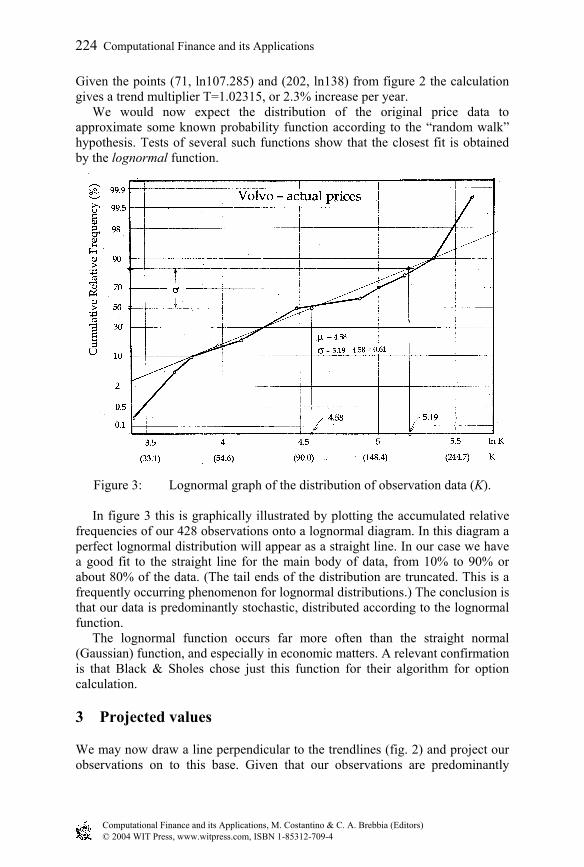
Given the points (71, ln107.285) and (202, ln138) from figure 2 the calculation gives a trend multiplier T=1.02315, or 2.3% increase per year. We would now expect the distribution of the original price data to approximate some known probability function according to the “random walk” hypothesis. Tests of several such functions show that the closest fit is obtained by the lognormal function.

Figure 3: Lognormal graph of the distribution of observation data (K).

In figure 3 this is graphically illustrated by plotting the accumulated relative frequencies of our 428 observations onto a lognormal diagram. In this diagram a perfect lognormal distribution will appear as a straight line. In our case we have a good fit to the straight line for the main body of data, from 10% to 90% or about 80% of the data. (The tail ends of the distribution are truncated. This is a frequently occurring phenomenon for lognormal distributions.) The conclusion is that our data is predominantly stochastic, distributed according to the lognormal function. The lognormal function occurs far more often than the straight normal (Gaussian) function, and especially in economic matters. A relevant confirmation is that Black & Sholes chose just this function for their algorithm for option calculation.

3 Projected values

We may now draw a line perpendicular to the trendlines (fig. 2) and project our observations on to this base. Given that our observations are predominantly



stochastic and lognormally distributed, our projected values will also be predominantly stochastic and lognormally distributed. However, our projected values will have an additional important characteristics, namely that all projected values lying on the same trendline will have the same projected value. Therefore, if there is a general systematic tendency for observations to line up in the trend direction, this should show in distributions. Projected prices can be computed using geometrical congruences:

Figure 4: Price projection. The baseline location is defined by the point ( )0,0 ln km , in this case (240, ln50). (The frequencies of the projected values are independent of the location of the baseline, which may therefore be arbitrarily positioned. This also means that the projected values as such do not have any absolute interpretation.) We have now three points as basis for computing projected values, ( ),ln, 11 km ( )22 ln, km defining the trend, and ( )00 ln, km defining the location of the baseline. Projected price values are denote by an asterisk (K*). As illustrated by figure 4 we have two congruent triangles with sides A, B, C and a, b, c respectively. We define the projected position of the first two points

on the ∗Kln -axis (the baseline) as akk +=∗0lnln where we have

BAba = . The

expressions may be simplified by interpreting α as a physical angle with tangent

12

12 lnlntanmm

kk−−

=α .

We then obtain: ( ) ( )( )( )αα coslnlntanlnln 011001 kkmmkk −+−+=∗



-and for the i-th point ( )ii km ln, : ( ) ( )( )( )αα coslnlntanlnln 000 kkmmkk iii −+−+=∗

According to figure 2 the values for 210 , kkk − are 50, 107.285 and 138

respectively, and for 21, mmmo − are 240, 70 and 202. Figure 5 shows the lognormal graphical presentation of the accumulated relative frequencies of (K*). For some reason the lognormal fit is considerably better than for the raw data, with parameters 84,4=µ and 49,0=σ . The dispersion of the distribution is also lower, with a standard deviation decreasing from 61,0=σ to 49,0=σ . (This remarkable improvement in fit and dispersion is probably a result of the better fit to the general tendency of the data, even with a trend multiplier as low as 1.02. One interesting aspect is its’ effect on calculated expected option value).

Figure 5: Lognormal graph of the distribution of projected data (K*).

4 Analysis

The analysis so far indicates that price movements are mainly stochastic and lognormally distributed. The question is whether there is a “trend bias” that may cause deviations from a purely stochastic behaviour. A first visual indication is obtained by drawing a simple histogram for increasing accumulated projected values in logarithmic form ( ∗kln ). Instead of obtaining an even curve, we get a curve broken by a number of steps of different



depth. This shows suites of equal or close to equal projected values, each such step indicating the existence of a “trendline”. A more general way of illustrate a possible “trend bias” would be to try to measure its effect on the stochastics itself. Given that the projected value (lnK*) is a stochastic variable (fig. 5), then the difference between consecutive projected values ∗

−∗ −=∆ 1lnln ii kk will also be a

stochastic variable. The same holds true for any difference ∗−

∗ −=∆ niin kk lnln . The classical definition of a trendline, three points on a line, corresponds to the requirement that the difference between three consecutive k*-values (column G, the data appendix) should be close to zero (in fact the difference can hardly ever be exactly zero, because the stock price K is a discrete and not a continuous variable. Stock prices are quoted in steps, the size of the steps depending upon the stock price level):

ε=−=∆ ∗−

∗22 ii kk

Now, because ∆ is a stochastic variable, the same holds true for the expected number of occurrences (B) within the interval )ln(ln 2

∗−

∗ − ii kk :

b= ( ) =≤≤∗ ∗∗∗− σµ,2 ii kKkPn ( )∫

∗

∗−

∗∗ik

kN kdkfn

2

ln,ln σµ

b ( ) ( )

−−−

−−= ∫ ∫

• ∗−

∗∗

∗∗

∗

∗

i ik k

dkkk

dkkk

n0 0

2

2

2

2 2

2lnexp1

2lnexp1

21

σµ

σµ

πσ

-where n is the total number of observations (428-2), with 84,4=µ and

49,0=σ according to figure 5. The value of the variable B may be computed for all ∗

ik . Being a lognormal stochastic variable, B will have a corresponding distribution function:

∫

−−=≤

0

02

2

0 2)(lnexp1

21),(

b

dbbb

bbPσµ

πσσµ

The hypothesis now says that if we have a “trend bias”, this should manifest itself in the form of a deviation from this “pure” stochastic distribution. If we have a condensation of occurrences around certain constant values (steps), the corresponding intervals will be narrower (with lower B values) than predicted by the distribution function, and we will thus expect to find that these low expected B values behave differently from the rest. Figure 6 shows the lognormal diagram of the accumulated relative frequencies of the B values. The figure shows a mixture of two lognormal distributions, both with a remarkably good fit of the empirical data (this excellent



fit holds true even at the utmost tails of the distributions, which is unusual. The first and the last points of the curve are each based upon only one single point (of 426), and the fit is still rather good). This means that our empirical data are drawn from two different populations, with b=0,9 as the dividing-line between the two. In other words, the expected deviation from the “pure” stochastic distribution is in itself a (“secondary”) stochastic distribution. The dominant (primary) distribution 9,0≥b represents 75% of the observations, with 3507,0=µ and 7141,0=σ . The theoretical average of the B values for this distribution is computed according to:

Figure 6: Lognormal graph of the projected price differences (B).

( ) ( )( ) ( ) ( ) ( )∫+∞

∞−

−−=== bdbbBEBEB ln

2lnexplnexp

21lnexp 2

2

σµ

πσ

( ) ( )( ) ( )bdb ln2

lnexp2

15,0exp 2

222 ∫

∞+

∞−

+−−+=

σσµ

πσσµ

( )2

5,0exp σµ +=

( ) 8323,142,190,2ln5,042,1lnexp

2

=

+=BE

The computed value of E(B) comes very close to the arithmetic mean of 1,89 of the computed B values. This primary distribution would probably not differ very



much from our concept of a “pure” distribution, that is a distribution without a “trend bias”. The second (secondary) distribution 9,0≤b , representing 25% of the observations, has totally different parameters: 6575,0=µ - and - 1342,1=σ with a theoretical average ( ) ( ) 6720,31342,1*5,06575,0exp 2 =+=BE . The accumulated frequencies at the low end of this secondary distribution are considerably higher than those that would have been obtained by the primary distribution in the same interval. This confirms the expected overrepresentation of low B values. The empirical approximations to the lognormal function have been tested according to the Kolmogorov-Smirnov criteria, and found significant on the 1%, 5% and 10% levels.

5 Conclusion

The Volvo case study indicates that stock prices behave according to the lognormal function. In other words, it is a stochastic variable as suggested by Bachelier. At the same time it appears that in this case we have a documented systematic tendency for prices to line up in a specific direction, a “trend bias”, which is in line with “Dow theory” and the trend concept. The equilibrium concept (the “random walk” hypothesis) and the trend concept have been in apparent contradiction for more than one hundred years. Could that conflict be resolved?

References

[1] Aitchison, J and J. A. C. Brown, 1957, “The Lognormal Distribution”, with special reference to its use in Rules”, Journal of Financial Economics, 51, 245-271.

[2] Bickel, Peter J. and Kjell A. Docksum, 2001, “Mathematical Statistics, Basic Ideas and Selected Topics”, Vol. 1, Prentice Hall, New Jersey 2001.

[3] Crow, Edwin L and Kunio Shimizu, 1988, “Lognormal Distributions, Theory and Applications” Marcel Dekker Inc., New York.

[4] Edwards, Robert D. and Magee, John, 1948, “Technical Analysis of Stock Trends”, John Magee inc., Boston 1948, sixteenth reprint 1997.

[5] Fowlkes, Edward B, 1979, “Some Methods for Studying the Mixture of Two Normal (Lognormal) Distributions”, Journal of the American Statistical Association, vol. 74, number 367, September 1979.

[6] Kendall, Maurice G., 1953, “The Analysis of Time Series, Part I: Prices”. Journal of the Royal Statistical Society, vol. 96.

[7] Lo, Andrew, Harry Mamaysky and Jiang Wang, 2000, “Foundations of Technical Analysis: Computational Algorithms, Statistical Inference, and Empirical Implementation”, The Journal of Finance, Vol. LV no. 4, August 2000.



price trends in speculative markets, do they exist? … · price trends in speculative markets, do...

Documents