Price Formation in Organized Wholesale Electricity Markets

Docket No. AD14-14-000

StaffAnalysisof

Operator‐InitiatedCommitments

inRTOandISOMarkets

December 2014

Forfurtherinformation,pleasecontact:

EmmaNicholsonOfficeofEnergyPolicyandInnovationFederalEnergyRegulatoryCommission

888FirstStreet,NEWashington,DC20426

(202)502‐8846emma.nicholson@ferc.gov

This report is a product of the Staff of the Federal Energy Regulatory Commission. The opinions and views expressed in this paper represent the preliminary analysis of

the Commission Staff. This report does not necessarily reflect the views of the Commission.

Table of Contents

Executive Summary ............................................................................................................. 1 

I.  Introduction ................................................................................................................... 3 

II.  Tools Used to Schedule Resources ........................................................................... 3 

A.  Security Constrained Unit Commitment ................................................................ 5 

B.  Security Constrained Economic Dispatch ............................................................. 8 

III.  Overview of Resource Scheduling Process ............................................................... 8 

A.  Day-Ahead Schedule............................................................................................ 10 

B.  Residual Unit Commitment Schedule .................................................................. 14 

C.  Real-time Schedule .............................................................................................. 18 

IV.  Locational Marginal Pricing .................................................................................... 22 

A.  Locational Marginal Pricing Overview ............................................................... 22 

B.  Cost Elements included in the LMP Framework ................................................. 25 

C.  EcoMin Relaxation .............................................................................................. 26 

D.  Fast-start Pricing Logic in RTOs and ISOs ......................................................... 28 

V.  Empirical Analysis .................................................................................................. 30 

A.  Methodology ........................................................................................................ 31 

B.  Results Overview ................................................................................................. 32 

C.  Market-specific Results ....................................................................................... 34 

VI.  Concluding Remarks ............................................................................................... 40 

1

ExecutiveSummary

This paper is part of an effort to evaluate matters affecting price formation in the energy and ancillary services markets operated by Regional Transmission Operators (RTOs) and Independent System Operators (ISOs) subject to the jurisdiction of the Federal Energy Regulatory Commission (FERC or Commission). It focuses on operator-initiated commitments in the RTOs and ISOs and the challenges in internalizing all relevant physical and operational constraints in the day-ahead and real-time market processes. This paper defines an operator-initiated commitment as a commitment that is not associated with a resource clearing the day-ahead or real-time market on the basis of economics and that is not a self-schedule. Deeming an action to be “operator-initiated” is not intended to confer any judgment that the action is not appropriate or necessary to maintain reliability.

Locational marginal prices (LMPs) for energy and ancillary services ideally would reflect the true marginal cost of production, taking into account all physical and operational system constraints, and fully compensate all resources for the variable cost of providing service.1 There are a number of challenges accounting for all physical and operational constraints. The central challenge stems from the fact that the full alternating current representation of the transmission system cannot currently be explicitly included in the market software despite the use of state-of-the-art computational tools. Further, some operational and reliability considerations can be difficult to incorporate into the day-ahead market process. Such considerations include managing the uncertainty related to real-time system conditions and resource performance or addressing local environmental constraints or secondary reliability concerns. As a result, alternative means are used to manage those elements that cannot be explicitly included in the day-ahead market process.

Two additional market design features related to developing prices that better reflect the actual operation of the system are what costs to include in the set of variable costs that are eligible to set clearing prices and which resources are eligible to set clearing prices. Specifically, there is some question whether some of the costs to commit resources are appropriately considered variable costs. This is particularly true for fast-start resources that can start-up quickly and typically have shorter minimum run times than other resources.2 A related question is how to ensure that fast-start resources are considered when setting price. Because fast-start resources are offline prior to being dispatched and then are typically dispatched immediately to their full operating limit, they can appear to

1 See Price Formation in Energy and Ancillary Services Markets Operated by Regional Transmission

Organizations and Independent System Operators, Notice, Docket No. AD14-14-000 (June 19, 2014).

2 The definition of fast-start resources varies across RTOs and ISOs.

2

be similar to resources committed out-of-market. As a result, RTOs and ISOs have to take steps to ensure the price setting algorithm recognizes these resources to allow them to be eligible to set the price.

This paper describes the processes RTOs and ISOs use to commit and dispatch resources in day-ahead and real-time, with a focus on how RTOs and ISOs address the market design challenges associated with difficult-to-model physical and operational constraints. A component of the discussion is how the market design decisions influence price formation. The extent of the price formation issues is somewhat dependent on the actual amount of capacity RTOs and ISOs are committing that is not reflected in energy and ancillary services prices. If RTOs and ISOs only commit a limited number of resources outside of the day-ahead or real-time market processes, then the price formation issues discussed would be largely theoretical. The paper concludes with an empirical analysis that attempts to measure the magnitude of certain types of operator-initiated commitments that are not directly reflected in market clearing prices.

This paper’s preliminary observations include the following:

All RTOs and ISOs have identified a class of reliability and operational issues that are incorporated into the day-ahead and real-time market processes but which are not reflected in day-ahead and real-time energy and ancillary services prices.

Some RTOs and ISOs have designed reserve products to address reliability and operational issues that would otherwise result in unit commitments outside of the day-ahead and real-time market processes.

The amount of capacity that is committed but not dispatched above a resource’s minimum operating level, a rough proxy for capacity that is not reflected in price, is moderate in most RTOs and ISOs but can reach fairly high levels in some hours.

Most RTOs and ISOs have some method to allow fast-start resources to set price, though the method used and the resources eligible to set price differ by market.

Some RTOs and ISOs allow the commitment costs of certain fast-start resources to be reflected in energy and ancillary services prices, though the costs included differ by market.

This paper is intended to spur discussion and lead to a more comprehensive understanding of operator-initiated actions and price formation. The workshop scheduled for December 9, 2014, will provide an opportunity for Commission Staff to learn the views of market participants, RTOs, ISOs, and market monitors.

3

I. Introduction

Energy and ancillary services markets are the primary mechanism that RTOs and ISOs use to identify the least-cost commitment and dispatch of system resources while respecting all applicable reliability standards. Because some relevant physical and operational constraints cannot, for reasons discussed below, be included in the market software, RTO and ISO operators also commit resources outside of the market clearing process to resolve reliability issues not internalized in the electricity and ancillary services markets. The market design choices that RTOs and ISOs make to best address the physical and operational constraints that are not included in the market software inherently influence price formation in the energy and ancillary service markets. The objective of this paper is to provide information and analysis relevant to a discussion of the extent to which out-of-market commitments made by RTOs and ISOs affect price formation in energy and ancillary services markets.

A critical first step in understanding the relationship between operator-initiated commitment and dispatch decisions and price formation is to develop an understanding of the framework under which unit commitment and dispatch decisions are typically made. This paper first provides a brief high level description of the primary software tools and business practices RTOs and ISOs use to control available generation (and other resources, where relevant) reliably and economically. Second, this paper presents an overview of the multi-stage process for scheduling and dispatching resources. In the process of presenting the overview, this paper highlights key market design decisions and how those decisions can influence price formation. Third, this paper reviews the process of setting LMP with a focus on the types of costs that are reflected in prices and the resources that are eligible to set price. Finally, the paper presents an empirical analysis of market data to identify and estimate the magnitude of certain types of operator-initiated commitments that are not directly reflected in market clearing prices.

II. Tools Used to Schedule Resources

A central function of RTOs and ISOs is to develop a schedule to coordinate the operation of all system resources. The schedule instructs all resources on the system when to start-up, how much electricity to generate while in operation, and when to shut down. The market operator follows a sequence of steps to select a least-cost mix of resources to reliably meet expected load conditions and to prepare the system to react to changing conditions effectively and economically, while respecting the constraints of the transmission system and the resources available to supply energy and ancillary services. The overarching goal of this process, from an economic viewpoint, is to maximize the social welfare while reliably serving load, where social welfare is measured as consumer

4

surplus plus producer surplus.3 Given the lack of price responsive demand, maximizing social welfare is primarily achieved by minimizing total production cost. The overarching goal from a reliability perspective is to comply with mandatory reliability standards as well as any local or supplemental reliability rules.

System operators use a suite of software tools to achieve these goals. These tools recognize that a resource must be committed – or started up – to be included in the schedule. Accordingly, developing a schedule typically involves two key decisions:

1) Unit commitment: the determination of which resources to start-up or shut-down and when to do so; and

2) Unit dispatch: the determination of the generation in megawatts (MW) each committed resource should produce in each interval.4

Unit commitment decisions are determined through an optimization process called security constrained unit commitment (SCUC). Unit dispatch is determined through a security constrained economic dispatch (SCED) optimization process. The phrase “security constrained” denotes the fact that the unit commitment and economic dispatch decisions are made subject to the condition that transmission system constraints are not violated and resource supply offer parameters and operating characteristics are honored. The two processes are explained in detail below.

There are a number of challenges to simultaneously maintaining reliability and minimizing production costs. First, the full alternating current representation of the transmission system cannot be explicitly included in the unit commitment and economic dispatch decisions given the current state-of-the-art computational tools.5 Specifically, voltage and stability constraints cannot be included in either the SCUC or SCED processes. As a result, alternative means, described below, must be used to avoid violating voltage and stability constraints. Second, the unit commitment and economic dispatch decisions are made before the uncertainty surrounding system conditions, including load, variable energy resource output, and generator performance is resolved. Again, alternative means in both day-ahead and real-time processes, described below, have been developed to manage this uncertainty. Third, some local reliability and operational rules can take the form of state or regional requirements to limit reliance on potentially scarce fuel or otherwise recognize environmental limitations.6 Some of these

3 Consumer surplus captures the fact that some consumers pay a price less than their maximum willingness to pay. Producer surplus captures the fact that some producers are paid a price greater than the marginal cost to produce electricity.

4 Demand-side resources are instructed to reduce load rather than increase generation.

5 Commission Staff’s annual Market Software Conference is intended to make progress on computational limitations. See http://www.ferc.gov/industries/electric/indus-act/market-planning.asp.

6 For example, NYISO implements the New York State Reliability Council’s Local Reliability Rules I-R3 and I-R5 by specifying minimum oil burn requirements for certain dual-fuel generators in New York City and Long

5

requirements can be included in the SCUC and SCED processes, but others are managed outside of these processes. And fourth, some system operators incorporate supplemental protocols designed to prepare resources to maintain reliability in the event that a secondary contingency occurs quickly after a primary contingency, so-called N-1-1 contingencies. These N-1-1 contingencies may be managed within or outside the SCUC and SCED processes. To the extent any of the above challenges are managed outside of the SCUC and SCED processes, it is difficult to ensure the resources selected in fact have the lowest production cost among all alternatives. In addition, any action taken to manage these issues that is not included in the SCUC and SCED processes will not be directly reflected in the energy and ancillary services prices. Un-modeled reliability requirements have an indirect effect on energy and ancillary service prices because these requirements commit additional units outside of the market construct, effectively adding supply, which could reduce clearing prices.

A. Security Constrained Unit Commitment

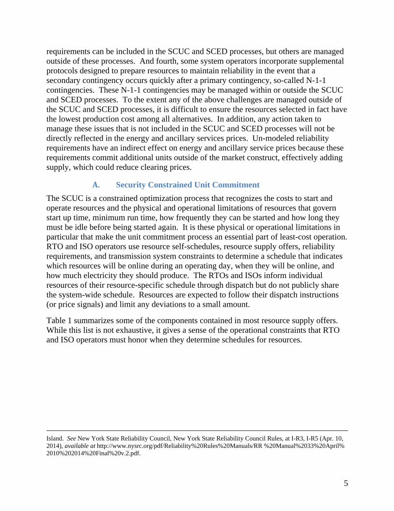
The SCUC is a constrained optimization process that recognizes the costs to start and operate resources and the physical and operational limitations of resources that govern start up time, minimum run time, how frequently they can be started and how long they must be idle before being started again. It is these physical or operational limitations in particular that make the unit commitment process an essential part of least-cost operation. RTO and ISO operators use resource self-schedules, resource supply offers, reliability requirements, and transmission system constraints to determine a schedule that indicates which resources will be online during an operating day, when they will be online, and how much electricity they should produce. The RTOs and ISOs inform individual resources of their resource-specific schedule through dispatch but do not publicly share the system-wide schedule. Resources are expected to follow their dispatch instructions (or price signals) and limit any deviations to a small amount.

Table 1 summarizes some of the components contained in most resource supply offers. While this list is not exhaustive, it gives a sense of the operational constraints that RTO and ISO operators must honor when they determine schedules for resources.

Island. See New York State Reliability Council, New York State Reliability Council Rules, at I-R3, I-R5 (Apr. 10, 2014), available at http://www.nysrc.org/pdf/Reliability%20Rules%20Manuals/RR %20Manual%2033%20April% 2010%202014%20Final%20v.2.pdf.

6

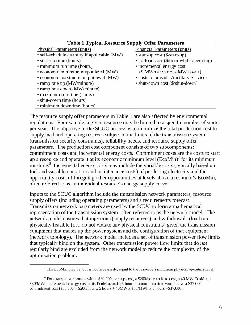
Table 1 Typical Resource Supply Offer Parameters Physical Parameters (units) Financial Parameters (units) • self-schedule quantity if applicable (MW) • start-up cost ($/start-up) • start-up time (hours) • no-load cost ($/hour while operating) • minimum run time (hours) • incremental energy cost • economic minimum output level (MW) ($/MWh at various MW levels) • economic maximum output level (MW) • costs to provide Ancillary Services • ramp rate up (MW/minute) • shut-down cost ($/shut-down) • ramp rate down (MW/minute) • maximum run-time (hours) • shut-down time (hours) • minimum downtime (hours)

The resource supply offer parameters in Table 1 are also affected by environmental regulations. For example, a given resource may be limited to a specific number of starts per year. The objective of the SCUC process is to minimize the total production cost to supply load and operating reserves subject to the limits of the transmission system (transmission security constraints), reliability needs, and resource supply offer parameters. The production cost component consists of two subcomponents: commitment costs and incremental energy costs. Commitment costs are the costs to start up a resource and operate it at its economic minimum level (EcoMin)7 for its minimum run-time.8 Incremental energy costs may include the variable costs (typically based on fuel and variable operation and maintenance costs) of producing electricity and the opportunity costs of foregoing other opportunities at levels above a resource’s EcoMin, often referred to as an individual resource’s energy supply curve.

Inputs to the SCUC algorithm include the transmission network parameters, resource supply offers (including operating parameters) and a requirements forecast. Transmission network parameters are used by the SCUC to form a mathematical representation of the transmission system, often referred to as the network model. The network model ensures that injections (supply resources) and withdrawals (load) are physically feasible (i.e., do not violate any physical constraints) given the transmission equipment that makes up the power system and the configuration of that equipment (network topology). The network model includes a set of transmission power flow limits that typically bind on the system. Other transmission power flow limits that do not regularly bind are excluded from the network model to reduce the complexity of the optimization problem.

7 The EcoMin may be, but is not necessarily, equal to the resource’s minimum physical operating level.

8 For example, a resource with a $30,000 start-up cost, a $200/hour no-load cost, a 40 MW EcoMin, a $30/MWh incremental energy cost at its EcoMin, and a 5 hour minimum run time would have a $37,000 commitment cost ($30,000 + $200/hour x 5 hours + 40MW x $30/MWh x 5 hours =$37,000).

7

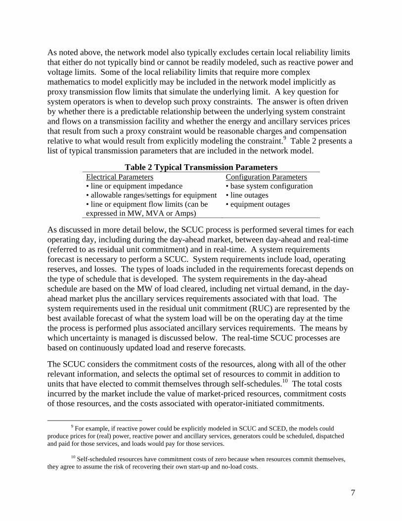
As noted above, the network model also typically excludes certain local reliability limits that either do not typically bind or cannot be readily modeled, such as reactive power and voltage limits. Some of the local reliability limits that require more complex mathematics to model explicitly may be included in the network model implicitly as proxy transmission flow limits that simulate the underlying limit. A key question for system operators is when to develop such proxy constraints. The answer is often driven by whether there is a predictable relationship between the underlying system constraint and flows on a transmission facility and whether the energy and ancillary services prices that result from such a proxy constraint would be reasonable charges and compensation relative to what would result from explicitly modeling the constraint.9 Table 2 presents a list of typical transmission parameters that are included in the network model.

Table 2 Typical Transmission Parameters Electrical Parameters Configuration Parameters • line or equipment impedance • base system configuration • allowable ranges/settings for equipment • line outages • line or equipment flow limits (can be expressed in MW, MVA or Amps)

• equipment outages

As discussed in more detail below, the SCUC process is performed several times for each operating day, including during the day-ahead market, between day-ahead and real-time (referred to as residual unit commitment) and in real-time. A system requirements forecast is necessary to perform a SCUC. System requirements include load, operating reserves, and losses. The types of loads included in the requirements forecast depends on the type of schedule that is developed. The system requirements in the day-ahead schedule are based on the MW of load cleared, including net virtual demand, in the day-ahead market plus the ancillary services requirements associated with that load. The system requirements used in the residual unit commitment (RUC) are represented by the best available forecast of what the system load will be on the operating day at the time the process is performed plus associated ancillary services requirements. The means by which uncertainty is managed is discussed below. The real-time SCUC processes are based on continuously updated load and reserve forecasts.

The SCUC considers the commitment costs of the resources, along with all of the other relevant information, and selects the optimal set of resources to commit in addition to units that have elected to commit themselves through self-schedules.10 The total costs incurred by the market include the value of market-priced resources, commitment costs of those resources, and the costs associated with operator-initiated commitments.

9 For example, if reactive power could be explicitly modeled in SCUC and SCED, the models could

produce prices for (real) power, reactive power and ancillary services, generators could be scheduled, dispatched and paid for those services, and loads would pay for those services.

10 Self-scheduled resources have commitment costs of zero because when resources commit themselves, they agree to assume the risk of recovering their own start-up and no-load costs.

8

B. Security Constrained Economic Dispatch

Like the SCUC, the SCED process is a constrained optimization problem. The SCED process determines how much electricity each committed resource in the schedule should generate, or hold in reserve as ancillary services.11 The SCED process uses much of the same information that is used in the SCUC, except that commitment cost data is not typically used. Energy and ancillary services dispatch levels are typically co-optimized in the SCED, meaning that the process simultaneously determines the optimal amounts of each.12 The SCED also calculates energy and ancillary services prices for the relevant market interval (hourly for the day-ahead market; and every five minutes for the real-time market). LMPs are calculated as the cost of serving the next increment of load at each location, and vary due to binding transmission constraints and losses. A similar calculation is made to price ancillary services. When calculated in this way, the ancillary services prices include the foregone profits that could have been earned from energy market sales, which represent a resource’s opportunity cost of providing ancillary services.

III. Overview of Resource Scheduling Process

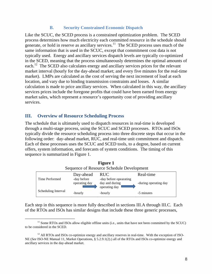
The schedule that is ultimately used to dispatch resources in real-time is developed through a multi-stage process, using the SCUC and SCED processes. RTOs and ISOs typically divide the resource scheduling process into three discrete steps that occur in the following order: day-ahead market, RUC, and real-time unit commitment and dispatch. Each of these processes uses the SCUC and SCED tools, to a degree, based on current offers, system information, and forecasts of system conditions. The timing of this sequence is summarized in Figure 1.

Figure 1 Sequence of Resource Schedule Development

Day-ahead RUC Real-time Time Performed

-day before operating day

-day before opearating day and during operating day

-during operating day

Scheduling Interval

-hourly -hourly -5 minutes

Each step in this sequence is more fully described in sections III.A through III.C. Each of the RTOs and ISOs has similar designs that include these three generic processes,

11 Some RTOs and ISOs allow eligible offline units (i.e., units that have not been committed by the SCUC)

to be considered in the SCED.

12 All RTOs and ISOs co-optimize energy and ancillary reserves in real-time. With the exception of ISO-NE (See ISO-NE Manual 11, Market Operations, § 5.2.9.1(2).) all of the RTOs and ISOs co-optimize energy and ancillary services in the day-ahead market.

9

although the timing, terminology, and details of each process vary. Resources can be included in the schedule in one of three ways: through a market clearing process on the basis of economics; through a self-schedule by the resource itself;13 or through an operator-initiated commitment. This paper defines an operator-initiated commitment as a commitment that is not associated with a resource clearing the day-ahead or real-time market on the basis of economics and that is not a self-schedule. Deeming an action to be “operator initiated” is not intended to confer any judgment that the action is not appropriate or necessary to maintain reliability. Rather, such actions are highlighted because they are not directly reflected in energy and ancillary services prices. Operator-initiated commitments can be made through automated out-of-market processes such as the RUC, or they can be made manually. For example, the RUC constitutes operator-initiated commitment because, although least-cost optimization is considered when decisions are made on operator-committed resources, the resources selected during the RUC are not included in the process used to set market clearing prices. Operators can also manually commit resources outside of the SCUC and SCED processes, as the driver of the decision is often a concern that is difficult to include in the SCUC or SCED processes, as discussed above. The following section first provides a high-level overview of the sequence of resource schedule development before discussing the steps in more detail and notes key differences across RTOs and ISOs.

The day-ahead schedule consists of unit commitment and dispatch instructions for every hour in the operating day based on the outcome of the day-ahead market clearing process.14 The day-ahead schedule consists of economic commitments, resource self-schedules, and operator-initiated commitments (if any). RTOs and ISOs amend the day-ahead schedule through a RUC that ensures that the day-ahead schedule contains enough generation to satisfy forecasted load and reserves. The RUC also addresses any reliability issues that are not sufficiently resolved in the day-ahead schedule. The real-time schedule further amends the RUC based on actual system conditions, the real-time market clearing process, self-schedules, and any operator-initiated commitments. The real-time schedule forms the basis of real-time commitment and dispatch instructions.

The RTOs and ISOs also have tariff provisions that permit operators to initiate changes to the schedule that are outside of either the day-ahead or real-time market process when

13 A self-scheduled resource submits its intended operating schedule as part of the day-ahead market

process; it is included in the SCUC and SCED as a resource with zero commitment costs and zero incremental energy costs at its self-scheduled quantity. Updates to a self-schedule may also be submitted in real-time and are processed in a similar manner. A resource owner’s decision to self-schedule is based on that entity’s view of its own economic best interest. The decision to self-schedule takes the commitment decision out of the SCUC process, which may have efficiency implications if that resource is not among the set of least cost resources.

14 The first step in developing a schedule is actually to determine which long-start resources will be needed on the operating day. Long-start resources need to be started prior to the day-ahead scheduling process because they have extended start-up times (e.g., 24 hours) and thus need to be notified earlier than units with shorter start-up times.

10

necessary to maintain system reliability or address issues not fully accounted for in the day-ahead, RUC, or real-time scheduling processes. Operators may manually commit resources to address concerns such as capacity shortages, generation or transmission contingencies, transmission facility overloads, or abnormal voltages. Operators may also manually commit resources for purposes such as avoiding load shedding, assisting neighboring areas, or mitigating other reliability issues.

A. Day-Ahead Schedule

All FERC-jurisdictional RTOs and ISOs have both a day-ahead and a real-time market. The day-ahead market is a daily forward market that takes place the day prior to the operating day to which it applies. The day-ahead market process balances supply offers (both physical and virtual) against demand bids (both physical and virtual).15 The day-ahead schedule is based on the load and ancillary services requirements that cleared the day-ahead market, including virtual supply and demand bids.16

Generally speaking, the day-ahead market clearing process employs a SCUC and SCED to dispatch energy and ancillary services in order to minimize total production costs subject to constraints in the network model and supply offers. The day-ahead SCUC and SCED optimization is dynamic in that it minimizes total production costs over the entire operating day. The day-ahead market process produces, for each hour of the relevant operating day, financially-binding schedules for all resources and loads that cleared the market and calculates energy and ancillary service clearing prices. For resources, this means that they are financially obligated to provide the quantity of MW that the resource cleared in the day-ahead schedule. For example, if a resource clears 100 MW through the day-ahead market in hour-ending 6:00, then it must either physically provide 100 MW during that hour at that location, purchase 100 MW from the real-time market during that hour at that location, or do some combination thereof.17 In addition to units that are scheduled through the day-ahead market, the day-ahead schedule includes self-scheduled resources and any resources previously committed through the long-start process.18

One common day-ahead market feature across all RTOs and ISOs is that demand bids and resource supply offers are due at a clearly stated time on the day before the operating

15 Virtual supply and demand offers are financial positions taken in the day-ahead market that settle based

on the difference between day-ahead and real-time clearing prices.

16 The day-ahead schedule is also likely to include resource commitments made through the RTO or ISO’s long-start commitment process. The long-start commitment process is necessary to commit resources with extended start-up times (e.g., 36 hours) that cannot be accommodated during the normal day-ahead market process.

17 In some markets, some resources have capacity obligations and would be expected to deliver scheduled energy except in the event of an unexpected outage.

18 The process that makes long-lead time commitments also involves economic considerations but it is separate from the formal centralized day-ahead or real-time markets.

11

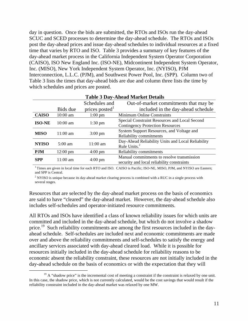
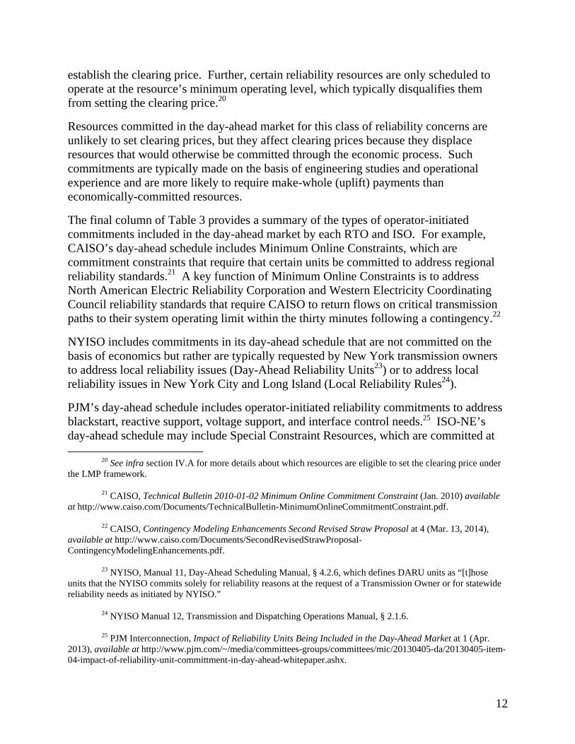
day in question. Once the bids are submitted, the RTOs and ISOs run the day-ahead SCUC and SCED processes to determine the day-ahead schedule. The RTOs and ISOs post the day-ahead prices and issue day-ahead schedules to individual resources at a fixed time that varies by RTO and ISO. Table 3 provides a summary of key features of the day-ahead market process in the California Independent System Operator Corporation (CAISO), ISO New England Inc. (ISO-NE), Midcontinent Independent System Operator, Inc. (MISO), New York Independent System Operator, Inc. (NYISO), PJM Interconnection, L.L.C. (PJM), and Southwest Power Pool, Inc. (SPP). Column two of Table 3 lists the times that day-ahead bids are due and column three lists the time by which schedules and prices are posted.

Table 3 Day-Ahead Market Details

Bids due Schedules and prices posted1

Out-of-market commitments that may be included in the day-ahead schedule

CAISO 10:00 am 1:00 pm Minimum Online Constraints

ISO-NE 10:00 am 1:30 pm Special Constraint Resources and Local Second Contingency Protection Resources

MISO 11:00 am 3:00 pm System Support Resources, and Voltage and Reliability commitments

NYISO 5:00 am 11:00 am Day-Ahead Reliability Units and Local Reliability Rule Units.2

PJM 12:00 pm 4:00 pm Reliability commitments

SPP 11:00 am 4:00 pm Manual commitments to resolve transmission security and local reliability constraints

1 Times are given in local time for each RTO and ISO. CAISO is Pacific; ISO-NE, MISO, PJM, and NYISO are Eastern; and SPP is Central.

2 NYISO is unique because its day-ahead market clearing process is combined with a RUC in a single process with several stages.

Resources that are selected by the day-ahead market process on the basis of economics are said to have “cleared” the day-ahead market. However, the day-ahead schedule also includes self-schedules and operator-initiated resource commitments.

All RTOs and ISOs have identified a class of known reliability issues for which units are committed and included in the day-ahead schedule, but which do not involve a shadow price.19 Such reliability commitments are among the first resources included in the day-ahead schedule. Self-schedules are included next and economic commitments are made over and above the reliability commitments and self-schedules to satisfy the energy and ancillary services associated with day-ahead cleared load. While it is possible for resources initially included in the day-ahead schedule for reliability reasons to be economic absent the reliability constraint, these resources are not initially included in the day-ahead schedule on the basis of economics or with the expectation that they will

19 A “shadow price” is the incremental cost of meeting a constraint if the constraint is relaxed by one unit. In this case, the shadow price, which is not currently calculated, would be the cost savings that would result if the reliability constraint included in the day-ahead market was relaxed by one MW.

12

establish the clearing price. Further, certain reliability resources are only scheduled to operate at the resource’s minimum operating level, which typically disqualifies them from setting the clearing price.20

Resources committed in the day-ahead market for this class of reliability concerns are unlikely to set clearing prices, but they affect clearing prices because they displace resources that would otherwise be committed through the economic process. Such commitments are typically made on the basis of engineering studies and operational experience and are more likely to require make-whole (uplift) payments than economically-committed resources.

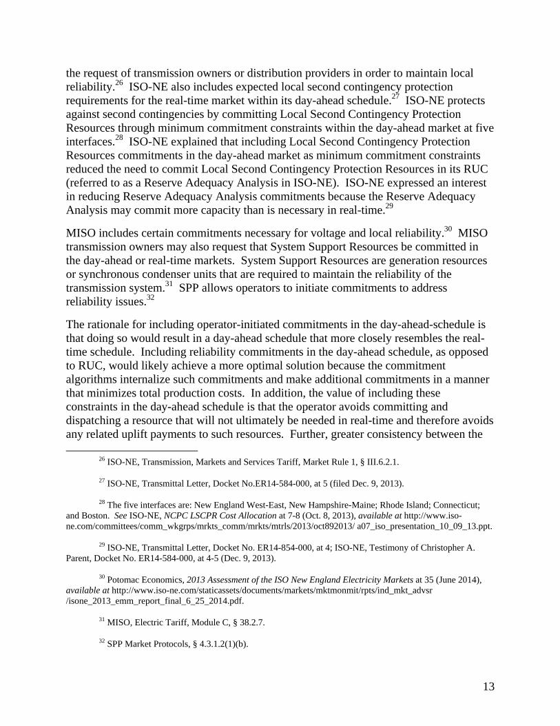
The final column of Table 3 provides a summary of the types of operator-initiated commitments included in the day-ahead market by each RTO and ISO. For example, CAISO’s day-ahead schedule includes Minimum Online Constraints, which are commitment constraints that require that certain units be committed to address regional reliability standards.21 A key function of Minimum Online Constraints is to address North American Electric Reliability Corporation and Western Electricity Coordinating Council reliability standards that require CAISO to return flows on critical transmission paths to their system operating limit within the thirty minutes following a contingency.22

NYISO includes commitments in its day-ahead schedule that are not committed on the basis of economics but rather are typically requested by New York transmission owners to address local reliability issues (Day-Ahead Reliability Units23) or to address local reliability issues in New York City and Long Island (Local Reliability Rules24).

PJM’s day-ahead schedule includes operator-initiated reliability commitments to address blackstart, reactive support, voltage support, and interface control needs.25 ISO-NE’s day-ahead schedule may include Special Constraint Resources, which are committed at

20 See infra section IV.A for more details about which resources are eligible to set the clearing price under the LMP framework.

21 CAISO, Technical Bulletin 2010-01-02 Minimum Online Commitment Constraint (Jan. 2010) available at http://www.caiso.com/Documents/TechnicalBulletin-MinimumOnlineCommitmentConstraint.pdf.

22 CAISO, Contingency Modeling Enhancements Second Revised Straw Proposal at 4 (Mar. 13, 2014), available at http://www.caiso.com/Documents/SecondRevisedStrawProposal-ContingencyModelingEnhancements.pdf.

23 NYISO, Manual 11, Day-Ahead Scheduling Manual, § 4.2.6, which defines DARU units as “[t]hose units that the NYISO commits solely for reliability reasons at the request of a Transmission Owner or for statewide reliability needs as initiated by NYISO.”

24 NYISO Manual 12, Transmission and Dispatching Operations Manual, § 2.1.6.

25 PJM Interconnection, Impact of Reliability Units Being Included in the Day-Ahead Market at 1 (Apr. 2013), available at http://www.pjm.com/~/media/committees-groups/committees/mic/20130405-da/20130405-item-04-impact-of-reliability-unit-committment-in-day-ahead-whitepaper.ashx.

13

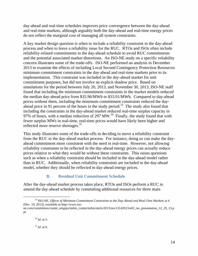
the request of transmission owners or distribution providers in order to maintain local reliability.26 ISO-NE also includes expected local second contingency protection requirements for the real-time market within its day-ahead schedule.27 ISO-NE protects against second contingencies by committing Local Second Contingency Protection Resources through minimum commitment constraints within the day-ahead market at five interfaces.28 ISO-NE explained that including Local Second Contingency Protection Resources commitments in the day-ahead market as minimum commitment constraints reduced the need to commit Local Second Contingency Protection Resources in its RUC (referred to as a Reserve Adequacy Analysis in ISO-NE). ISO-NE expressed an interest in reducing Reserve Adequacy Analysis commitments because the Reserve Adequacy Analysis may commit more capacity than is necessary in real-time.29

MISO includes certain commitments necessary for voltage and local reliability.30 MISO transmission owners may also request that System Support Resources be committed in the day-ahead or real-time markets. System Support Resources are generation resources or synchronous condenser units that are required to maintain the reliability of the transmission system.31 SPP allows operators to initiate commitments to address reliability issues.32

The rationale for including operator-initiated commitments in the day-ahead-schedule is that doing so would result in a day-ahead schedule that more closely resembles the real-time schedule. Including reliability commitments in the day-ahead schedule, as opposed to RUC, would likely achieve a more optimal solution because the commitment algorithms internalize such commitments and make additional commitments in a manner that minimizes total production costs. In addition, the value of including these constraints in the day-ahead schedule is that the operator avoids committing and dispatching a resource that will not ultimately be needed in real-time and therefore avoids any related uplift payments to such resources. Further, greater consistency between the

26 ISO-NE, Transmission, Markets and Services Tariff, Market Rule 1, § III.6.2.1.

27 ISO-NE, Transmittal Letter, Docket No.ER14-584-000, at 5 (filed Dec. 9, 2013).

28 The five interfaces are: New England West-East, New Hampshire-Maine; Rhode Island; Connecticut; and Boston. See ISO-NE, NCPC LSCPR Cost Allocation at 7-8 (Oct. 8, 2013), available at http://www.iso-ne.com/committees/comm_wkgrps/mrkts_comm/mrkts/mtrls/2013/oct892013/ a07_iso_presentation_10_09_13.ppt.

29 ISO-NE, Transmittal Letter, Docket No. ER14-854-000, at 4; ISO-NE, Testimony of Christopher A. Parent, Docket No. ER14-584-000, at 4-5 (Dec. 9, 2013).

30 Potomac Economics, 2013 Assessment of the ISO New England Electricity Markets at 35 (June 2014), available at http://www.iso-ne.com/staticassets/documents/markets/mktmonmit/rpts/ind_mkt_advsr /isone_2013_emm_report_final_6_25_2014.pdf.

31 MISO, Electric Tariff, Module C, § 38.2.7.

32 SPP Market Protocols, § 4.3.1.2(1)(b).

14

day-ahead and real-time schedules improves price convergence between the day-ahead and real-time markets, although arguably both the day-ahead and real-time energy prices do not reflect the marginal cost of managing all system constraints.

A key market design question is when to include a reliability constraint in the day-ahead process and when to leave a reliability issue for the RUC. RTOs and ISOs often include reliability-related commitments in the day-ahead schedule to avoid RUC commitments and the potential associated market distortions. An ISO-NE study on a specific reliability concern illustrates some of the trade-offs. ISO-NE performed an analysis in December 2013 to examine the effects of including Local Second Contingency Protection Resources minimum commitment constraints in the day-ahead and real-time markets prior to its implementation. This constraint was included in the day-ahead market for unit commitment purposes, but did not involve an explicit shadow price. Based on simulations for the period between July 20, 2013, and November 30, 2013, ISO-NE staff found that including the minimum commitment constraints in the market models reduced the median day-ahead price from $35.96/MWh to $33.91/MWh. Compared to day-ahead prices without them, including the minimum commitment constraints reduced the day-ahead price in 91 percent of the hours in the study period.33 The study also found that including the constraints in the day-ahead market reduced real-time surplus capacity in 97% of hours, with a median reduction of 297 MW.34 Finally, the study found that with fewer surplus MWs in real-time, real-time prices would have likely been higher and reflected more reserve shortages.35

This study illustrates some of the trade-offs in deciding to move a reliability constraint from the RUC to the day-ahead market process. For instance, doing so can make the day-ahead commitment more consistent with the need in real-time. However, not allowing reliability constraints to be reflected in the day-ahead energy prices can actually reduce prices relative to what they would be without these constraints. This raises questions such as when a reliability constraint should be included in the day-ahead model rather than in RUC. Additionally, when reliability constraints are included in the day-ahead model, whether they should be reflected in day-ahead energy prices.

B. Residual Unit Commitment Schedule

After the day-ahead market process takes place, RTOs and ISOs perform a RUC to amend the day-ahead schedule by committing additional resources for three main

33 ISO-NE, Effects of Minimum Commitment Constraints to the Day-Ahead and Real-Time Markets at 4

(Dec. 19, 2013), available at http://www.iso-ne.com/committees/comm_wkgrps/mrkts_comm/mrkts/mtrls/2013/nov13142013/a03_iso_presentation_12_19_13.ppt.

34 Id. at 5.

35 Id. at 6.

15

reasons: (1) resource gaps; (2) reliability issues; and (3) to manage uncertainty and the potential for real-time operational issues (e.g., ramping). Resource gaps occur when the demand cleared in the day-ahead market is below the RTO’s or ISO’s demand forecast for the operating day. Day-ahead cleared load may be below the demand forecast for a variety of reasons, ranging from weather and load forecast uncertainty to conscious decisions by load serving entities to leave a certain portion of their load unhedged and to purchase in the real-time market. Net virtual supply positions can also cause resource gaps because they offset physical demand cleared in the day-ahead market.

The RUC also includes commitments to address reliability issues that are not resolved in the day-ahead schedule. The day-ahead schedule will have unresolved reliability issues if the model that underlies the day-ahead market does not include all relevant reliability constraints. Voltage constraints and other local reliability requirements are significant drivers of reliability-related RUC commitments. For example, a particular transmission area may contain an un-modeled local reactive power constraint that affects a sub-area within the greater transmission area. This can occur when a single high cost resource is the only resource that can resolve a reactive power issue that is not enforced in the day-ahead market. The day-ahead market may not commit this high cost resource economically because the local reactive power constraint is not included in the network model. Instead, the day-ahead market clearing process will commit and dispatch the least expensive resources in the larger area. If the resource needed to meet this local reliability requirement does not clear in the day-ahead market, it must be committed to maintain reliability so the operator will ensure that it is committed either through an automated algorithm or manually. As noted in a previous FERC staff paper, certain resources are consistently committed outside of the market to address reliability issues, which results in concentrated uplift payments.36

The RUC typically maintains the commitment and dispatch decisions in the day-ahead schedule and either increases the dispatch levels of units already included in the day-ahead schedule or makes additional commitments to address resource gaps and reliability issues. While exact practices differ by RTO and ISO, the RUC is based on a unit commitment process that minimizes the additional residual commitment costs (i.e., start-up and no-load costs, without consideration of any variable costs) associated with any incremental commitments beyond the day-ahead schedule.37

To shed further light on how commitments made in the RUC are reflected in prices, it’s informative to note that, while CAISO, ISO-NE, MISO, PJM, and SPP complete the

36 See Federal Energy Regulatory Commission, Staff Analysis of Uplift in RTO and ISO Markets (Aug.

2014), available at http://www.ferc.gov/legal/staff-reports/2014/08-13-14-uplift.pdf (containing discussion and analysis concerning uplift).

37 If day-ahead cleared load is higher than the load forecast, the RUC may remove – or decommit – resources from the day-ahead schedule.

16

RUC after the day-ahead market clearing process ends, NYISO’s RUC is integrated within its multi-step day-ahead market process. This design results in day-ahead prices that reflect RUC commitments. The first step of NYISO’s day-ahead market process selects resources to satisfy cleared load and reserve requirements, which is similar to the other RTOs and ISOs. However, NYISO’s day-ahead market process continues to an additional step that commits additional resources (if necessary) to satisfy the load forecast and reliability issues, a traditional function of the RUC. Additional passes in NYISO’s day-ahead market software incorporate the resources committed in the second pass of the day-ahead market (a RUC) to determine the final day-ahead schedule and clearing prices.38 As a result, NYISO’s day-ahead schedule and prices reflect commitments made in RUC.

Operators may commit additional resources in RUC to address uncertainty and the potential for real-time operational issues (e.g., ramping). For example, operators may assess that the uncertainty surrounding either supply-side or demand-side factors warrant the commitment of additional resources over and above the resources necessary to satisfy the load forecast. For example, operators may determine that a resource included in the day-ahead schedule has a high probability of experiencing a forced outage and consequently increase the capacity requirement used in the RUC or manually add additional commitments to the RUC results. Such adjustments are made at the discretion of the operators.

Some RTOs and ISOs have added a class of RUC commitments to manage this uncertainty and potential for real-time operational issues. For instance, MISO’s RUC, referred to as a Forward Reliability Assessment Commitment, includes a requirement that the system have sufficient Headroom and Floorroom.39 Headdroom constraints may also be included in the MISO’s day-ahead market.40 Headroom is an upward ramping capacity requirement to accommodate load increases that can be satisfied by either unloaded generation or fast-start units. Floorroom, defined similarly, is downward ramping capability. MISO defines headroom as the greater of the (1) unloaded capacity requirement (which is currently 750 MW); and (2) sixty percent of the hourly change in load.41 Similarly, during SPP’s day-ahead market and RUC, operators also ensure that

38 NYISO Manual 11, Day-Ahead Scheduling Manual, § 4.3.1; NYISO, NYISO Day-Ahead Market

Overview at 12-14 (Jun. 28-29, 2010), available at http://www.ferc.gov/CalendarFiles/20110628072825-Jun28-SesA1-Johnson-NYISO.pdf.

39 MISO Tariff Module A, § II.1H; MISO Tariff Module A, § II.1F.

40 MISO, Ramp Capability Product Design for MISO Markets at 12 (Dec. 22, 2013), available at https://www.misoenergy.org/Library/Repository/Communication%20Material/Key%20Presentations%20and%20Whitepapers/Ramp%20Capability%20for%20Load%20Following%20in%20MISO%20Markets%20White%20Paper.pdf.

41 MISO, FERC Electric Tariff, Module C, § 40.3.3 (10.0.0). See also page 3 of MISO’s November 22, 2013 written answers in the Technical Conference in Docket No. ER13-2124-000.

17

the system has sufficient upward ramping capacity (referred to as head-room requirements) and downward ramp capacity (referred to as floor-room requirements).42

The Commission recently approved MISO’s proposed ramp capability product, which will procure some of the capability MISO currently includes in its Headroom and Floorroom requirements in the day-ahead and real-time markets.43 MISO plans to procure Up Ramp and Down Ramp capability through the market by adding a constraint to both the day-ahead and real-time market models that specifies the desired ramp capability necessary to address short-term variations in net load.44

Some RTOs and ISOs have taken steps to replace certain RUC commitments with reserve products to better reflect the costs of such commitments in the day-ahead and real-time clearing prices for ancillary services. For example, in an effort to improve day-ahead and real-time price formation, in 2013 ISO-NE included in its day-ahead market a co-optimized replacement reserve product to procure in the market-clearing process resources that had previously been procured as operator-initiated RUC commitments. ISO-NE’s replacement reserve requirement is 160 MW in the summer and 180 MW in the winter.45 As such, the replacement reserve requirements are reflected in ISO-NE’s forward reserves market, day-ahead energy market and real-time energy market.

PJM’s Market Service Committee recently approved a similar approach that instructs operators to increase the hourly day-ahead scheduling reserve obligation in the day-ahead market during hot and cold weather alerts and maximum generation alerts.46 PJM explained that the motivation for this proposal was to better reflect the costs of the reserves in clearing prices.47 Another key market design question is when a commitment that has traditionally been part of the RUC can be converted into a reserve product.

The objective of the RUC in all of the RTOs and ISOs is to minimize the incremental residual commitment costs of any additional capacity that is committed, based on resource energy offers submitted into the day-ahead or during the RUC-rebid period. CAISO’s RUC is unique because CAISO allows resources to submit a capacity bid,

42 SPP OATT, attach. AE, § 5.1.1(11); SPP OATT, attach. AE, § 5.2.1(17).

43 Midcontinent Indep. Sys. Operator, Inc., 149 FERC ¶ 61,095, at P 5 (2014).

44 Id. P 6. Net load is physical load minus generation from variable resources.

45 ISO New England, Inc., Transmittal Letter, Docket No. ER13-1736-000, at 10 (filed June 10, 2013).

46 PJM, Energy and Reserve Pricing & Interchange Volatility Final Proposal Report at 2 (Oct. 30, 2014), available at http://www.pjm.com/~/media/committees-groups/committees/mrc/20141030/20141030-item-04-erpiv-final-proposal-report.ashx.

47 Id. Rather than a fixed amount, the additional reserves would be based on demand as adjusted by a “seasonal conditional demand factor” – based on actual demand during the peak hours for the top 10 peak load days in the same season the prior year.

18

referred to as a RUC Availability bid, for any capacity not committed as part of the day-ahead market.48 When a resource submits a RUC Availability bid, it is offering to submit a supply offer for a specific MW quantity of supply to the real-time market during a specific hour (or hours). If a resource’s RUC Availability bid is accepted, it must offer a MW quantity equal to its RUC award in to the real-time energy market during the hour of its award. The RUC Availability bids do not specify the $/MWh level that the resource will offer into the real-time market - they only specify that a real-time offer will be made.49 CAISO uses the RUC Availability bids to select resources to minimize incremental commitment costs.50 In doing so, CAISO calculates a RUC price that is separate from the day-ahead energy and ancillary service clearing prices. 51 The RUC awards are similar to a capacity payment as they serve to guarantee that the resource will offer capacity equal to its RUC award in to the real-time market. CAISO’s internal market monitor found that most of its RUC awards do not create additional generation in real-time.52 The costs associated with CAISO’s RUC are treated similar to uplift and collected through a side payment that is allocated across two tiers.53

C. Real-time Schedule

The day-ahead schedule, as amended by the RUC, forms the basis of real-time operations. The real-time schedule gives resources instructions to deviate from their day-ahead schedule as required by real-time conditions. Throughout real-time, the RTO and ISO system operators maintain the balance between supply and demand for energy and reserves by issuing dispatch instructions that either commit resources, decommit resources, or instruct resources that are currently operating to ramp up or down.54 Real-

48 CAISO eTariff, § 31.5.1.1.

49 CAISO Department of Market Monitoring, 2013 Annual Report on Market Issues & Performance at 102 (Apr. 2014), available at http://www.caiso.com/Documents/2013AnnualReport-MarketIssue-Performance.pdf.

50 See CAISO eTariff, § 31.5.

51 See id., § 31.5.1.4.

52 CAISO Department of Market Monitoring, 2013 Annual Report on Market Issues & Performance at 101 (Apr. 2014), available at http://www.caiso.com/Documents/2013AnnualReport-MarketIssue-Performance.pdf.

53 Resource Adequacy resources in CAISO must submit zero cost RUC Availability bids (i.e., $0/MW). RUC costs are driven by RUC Availability Payments and any uplift associated with the RUC awards. Day-Ahead RUC Tier 1 costs are allocated to virtual suppliers if in aggregate, the day-ahead cleared net virtual supply amount is positive. Any remaining RUC costs are allocated pro rata to metered load through a Day-Ahead RUC Tier 2 allocation. California ISO, Settlement & Billing Internal Configuration Guide: CG CC06806 Day-Ahead Residual Unit Commitment (RUC) Tier 1 Allocation 3 (Sept. 2014 ), available at http://bpmcm.caiso.com/BPM%20Document%20Library/Settlements%20and%20Billing/Configuration%20Guides/Cost%20Recovery/BPM%20-%20CG%20CC%206806%20Day%20Ahead%20Residual%20Unit%20Commitment%20(RUC)%20Tier%201%20Allocation_5.7.doc.

54 To decommit a resource means to instruct it to shut down.

19

time dispatch instructions are developed throughout the operating day – typically every five minutes – to optimally commit and/or dispatch resources at least-cost to manage real-time conditions and maintain reliability. Operators may perform additional RUCs in real-time that are similar to the day-ahead RUC for the hours remaining in the operating day with updated inputs that reflect prevailing system conditions. Operators in all of the RTOs and ISOs also have additional vehicles to make out-of-market commitments. For example, exceptional dispatches55 in CAISO, Out-of-Merit generation56 in NYISO, and Balancing Operating Reserves57 in PJM.

In addition to these standard real-time dispatch operations, some markets also run parallel “look-ahead” processes that guide dispatch for the periods beyond the next interval. The motivation for a multi-period look-ahead is to overcome the shortcomings of the single-period optimization that typically forms the basis of real-time dispatch. Multi-period look-ahead processes attempt to make optimal choices over a longer time-span, and can often result in commitment and dispatch solutions that are less costly than single-period optimizations. A single-period optimization only makes decisions based on the immediate future (typically the next five to fifteen minutes). This short-term single-period optimization fails to consider changes in system conditions beyond the upcoming period.

For example, suppose that updated load forecasts in real-time are for three hours in the future significantly higher than the load assumed in the day-ahead schedule and RUC. Two available options that satisfy this future load growth are: (1) commit an expensive fast-start resource immediately prior to the load increase; and (2) commit a less expensive medium-start58 resource in the next one or two hours. It may be cheaper to commit the medium-start resource to serve load that is expected to materialize in the next three hours, but a short-term/single-period optimization will not do so because the load increase does not happen within the short-term optimization period. In contrast, a multi-period look-ahead optimization may realize the benefit of committing the medium-start resource instead of the fast-start resource. The look-ahead processes typically involve a rolling SCED, SCUC, or both that continuously evaluate system conditions in anticipation of future events and future operating periods. The look-ahead processes serve as guides for subsequent real-time dispatch instructions.

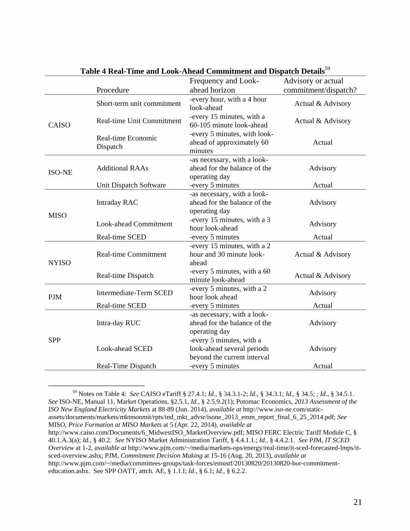
Table 4 summarizes the dispatch and look-ahead processes that operators use in real-time to assist them in making optimal unit-commitment and dispatch decisions. Note that in all RTOs and ISOs, real-time SCEDs, often referred to as real-time dispatch processes,

55 CAISO eTariff, § 34.11.

56 NYISO, Manual 12 Transmission and Dispatching Operations, § 5.7.4.

57 PJM, Intra-PJM Tariff, OATT, attach. K, § 3.2.3.

58 Medium-start resources can be started up fairly quickly but not as quickly as fast-start resources.

20

issue dispatch instructions. The period of time included in the forward look-ahead is referred to as the “look-ahead horizon” or “forecast period.” Rather than automatically following the recommendations of the look-ahead tools, operators also have discretion about which resources to ultimately commit and dispatch in real-time.

The look-ahead process typically creates both actual and advisory dispatch and prices. Typically, the first period of the multi-period look-ahead optimization is used to set prices and create dispatch instructions, while the remaining periods of the optimization are advisory. The last column of Table 4 indicates whether the real-time process produces actual dispatch instructions and calculates real-time prices or is used for advisory purposes only.

21

Table 4 Real-Time and Look-Ahead Commitment and Dispatch Details59

Procedure

Frequency and Look-ahead horizon

Advisory or actual commitment/dispatch?

CAISO

Short-term unit commitment -every hour, with a 4 hour look-ahead

Actual & Advisory

Real-time Unit Commitment -every 15 minutes, with a 60-105 minute look-ahead

Actual & Advisory

Real-time Economic Dispatch

-every 5 minutes, with look-ahead of approximately 60 minutes

Actual

ISO-NE Additional RAAs

-as necessary, with a look-ahead for the balance of the operating day

Advisory

Unit Dispatch Software -every 5 minutes Actual

MISO

Intraday RAC -as necessary, with a look-ahead for the balance of the operating day

Advisory

Look-ahead Commitment -every 15 minutes, with a 3 hour look-ahead

Advisory

Real-time SCED -every 5 minutes Actual

NYISO Real-time Commitment

-every 15 minutes, with a 2 hour and 30 minute look-ahead

Actual & Advisory

Real-time Dispatch -every 5 minutes, with a 60 minute look-ahead

Actual & Advisory

PJM Intermediate-Term SCED

-every 5 minutes, with a 2 hour look ahead

Advisory

Real-time SCED -every 5 minutes Actual

SPP

Intra-day RUC -as necessary, with a look-ahead for the balance of the operating day

Advisory

Look-ahead SCED -every 5 minutes, with a look-ahead several periods beyond the current interval

Advisory

Real-Time Dispatch -every 5 minutes Actual

59 Notes on Table 4: See CAISO eTariff § 27.4.1; Id., § 34.3.1-2; Id., § 34.3.1; Id., § 34.5; ; Id., § 34.5.1.

See ISO-NE, Manual 11, Market Operations, §2.5.1, Id., § 2.5.9.2(1); Potomac Economics, 2013 Assessment of the ISO New England Electricity Markets at 88-89 (Jun. 2014), available at http://www.iso-ne.com/static-assets/documents/markets/mktmonmit/rpts/ind_mkt_advsr/isone_2013_emm_report_final_6_25_2014.pdf; See MISO, Price Formation at MISO Markets at 5 (Apr. 22, 2014), available at http://www.caiso.com/Documents/6_MidwestISO_MarketOverview.pdf; MISO FERC Electric Tariff Module C, § 40.1.A.3(a); Id., § 40.2. See NYISO Market Administration Tariff, § 4.4.1.1.; Id., § 4.4.2.1. See PJM, IT SCED Overview at 1-2, available at http://www.pjm.com/~/media/markets-ops/energy/real-time/it-sced-forecasted-lmps/it-sced-overview.ashx; PJM, Commitment Decision Making at 15-16 (Aug. 20, 2013), available at http://www.pjm.com/~/media/committees-groups/task-forces/emustf/20130820/20130820-bor-commitment-education.ashx. See SPP OATT, attch. AE, § 1.1.I; Id., § 6.1; Id., § 6.2.2.

22

IV. Locational Marginal Pricing

LMP is central to price formation in RTOs and ISOs.60 Two key issues associated with LMP, operator-initiated actions and the SCUC and SCED processes, are highlighted. The first issue is what types of costs are included in the LMP. The second issue is which resources are eligible to set the price. Energy prices may be distorted to the extent a resource is committed and dispatched to provide energy but is not eligible to set the price. The primary challenge is determining whether energy prices should reflect just resource incremental energy offers or whether energy prices should also include some or all of a resource’s start-up and no-load costs. The issue is connected to the operator-initiated actions issues discussed earlier because the decision to include system constraints in the RUC, and not the day-ahead or real-time market’s SCUC process, will influence whether commitment costs can be reflected in energy prices.

Section IV.A provides an overview of LMP, section IV.B discusses the issue of what costs to include in setting energy and ancillary services prices, section IV.C explains how LMP can be amended for fast-start resources, and section IV.D summarizes fast-start pricing logic in FERC-jurisdictional RTOs and ISOs.

A. Locational Marginal Pricing Overview

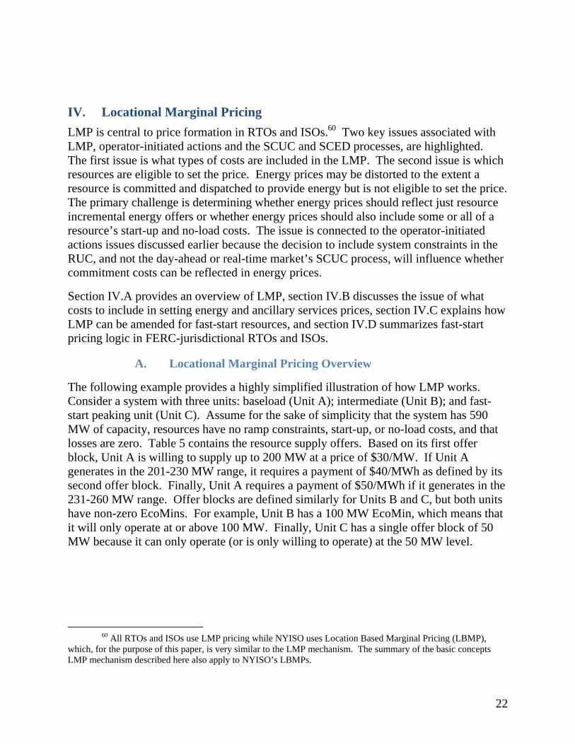
The following example provides a highly simplified illustration of how LMP works. Consider a system with three units: baseload (Unit A); intermediate (Unit B); and fast-start peaking unit (Unit C). Assume for the sake of simplicity that the system has 590 MW of capacity, resources have no ramp constraints, start-up, or no-load costs, and that losses are zero. Table 5 contains the resource supply offers. Based on its first offer block, Unit A is willing to supply up to 200 MW at a price of $30/MW. If Unit A generates in the 201-230 MW range, it requires a payment of $40/MWh as defined by its second offer block. Finally, Unit A requires a payment of $50/MWh if it generates in the 231-260 MW range. Offer blocks are defined similarly for Units B and C, but both units have non-zero EcoMins. For example, Unit B has a 100 MW EcoMin, which means that it will only operate at or above 100 MW. Finally, Unit C has a single offer block of 50 MW because it can only operate (or is only willing to operate) at the 50 MW level.

60 All RTOs and ISOs use LMP pricing while NYISO uses Location Based Marginal Pricing (LBMP),

which, for the purpose of this paper, is very similar to the LMP mechanism. The summary of the basic concepts LMP mechanism described here also apply to NYISO’s LBMPs.

23

Table 5 Example of LMP Mechanics Unit Block 1 Block 2 Block 3 Total MW range $/MWh MW range $/MWh MW range $/MWh MW A 0-200 $30 201-230 $40 231-260 $50 260 B 100 $70 101-140 $90 141-180 $150 180 C 50 $200 50

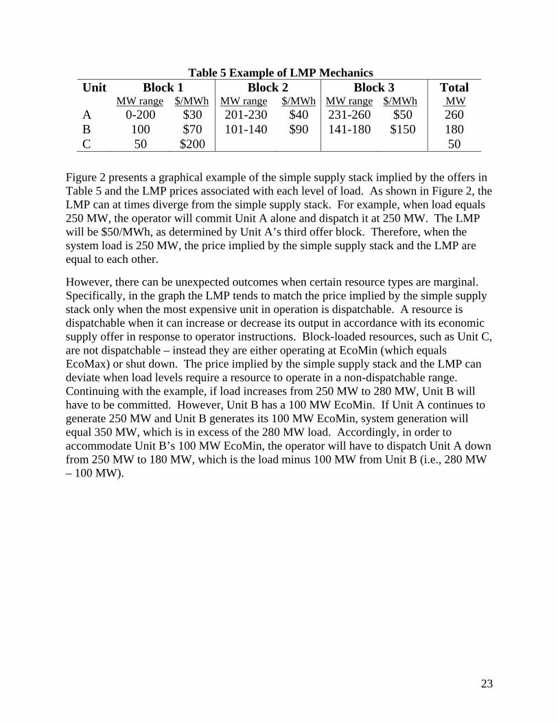
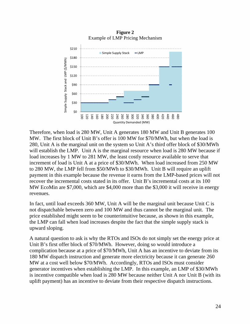
Figure 2 presents a graphical example of the simple supply stack implied by the offers in Table 5 and the LMP prices associated with each level of load. As shown in Figure 2, the LMP can at times diverge from the simple supply stack. For example, when load equals 250 MW, the operator will commit Unit A alone and dispatch it at 250 MW. The LMP will be $50/MWh, as determined by Unit A’s third offer block. Therefore, when the system load is 250 MW, the price implied by the simple supply stack and the LMP are equal to each other.

However, there can be unexpected outcomes when certain resource types are marginal. Specifically, in the graph the LMP tends to match the price implied by the simple supply stack only when the most expensive unit in operation is dispatchable. A resource is dispatchable when it can increase or decrease its output in accordance with its economic supply offer in response to operator instructions. Block-loaded resources, such as Unit C, are not dispatchable – instead they are either operating at EcoMin (which equals EcoMax) or shut down. The price implied by the simple supply stack and the LMP can deviate when load levels require a resource to operate in a non-dispatchable range. Continuing with the example, if load increases from 250 MW to 280 MW, Unit B will have to be committed. However, Unit B has a 100 MW EcoMin. If Unit A continues to generate 250 MW and Unit B generates its 100 MW EcoMin, system generation will equal 350 MW, which is in excess of the 280 MW load. Accordingly, in order to accommodate Unit B’s 100 MW EcoMin, the operator will have to dispatch Unit A down from 250 MW to 180 MW, which is the load minus 100 MW from Unit B (i.e., 280 MW – 100 MW).

24

Figure 2 Example of LMP Pricing Mechanism

Therefore, when load is 280 MW, Unit A generates 180 MW and Unit B generates 100 MW. The first block of Unit B’s offer is 100 MW for $70/MWh, but when the load is 280, Unit A is the marginal unit on the system so Unit A’s third offer block of $30/MWh will establish the LMP. Unit A is the marginal resource when load is 280 MW because if load increases by 1 MW to 281 MW, the least costly resource available to serve that increment of load is Unit A at a price of $30/MWh. When load increased from 250 MW to 280 MW, the LMP fell from $50/MWh to $30/MWh. Unit B will require an uplift payment in this example because the revenue it earns from the LMP-based prices will not recover the incremental costs stated in its offer. Unit B’s incremental costs at its 100 MW EcoMin are $7,000, which are $4,000 more than the $3,000 it will receive in energy revenues.

In fact, until load exceeds 360 MW, Unit A will be the marginal unit because Unit C is not dispatchable between zero and 100 MW and thus cannot be the marginal unit. The price established might seem to be counterintuitive because, as shown in this example, the LMP can fall when load increases despite the fact that the simple supply stack is upward sloping.

A natural question to ask is why the RTOs and ISOs do not simply set the energy price at Unit B’s first offer block of $70/MWh. However, doing so would introduce a complication because at a price of $70/MWh, Unit A has an incentive to deviate from its 180 MW dispatch instruction and generate more electricity because it can generate 260 MW at a cost well below $70/MWh. Accordingly, RTOs and ISOs must consider generator incentives when establishing the LMP. In this example, an LMP of $30/MWh is incentive compatible when load is 280 MW because neither Unit A nor Unit B (with its uplift payment) has an incentive to deviate from their respective dispatch instructions.

$0

$30

$60

$90

$120

$150

$180

$210

100

120

140

160

180

200

220

240

260

280

300

320

340

360

380

400

420

440

460

480

Simple Supply  Stack and  LMP ($/M

Wh)

Quantity Demanded (MW)

Simple Supply Stack LMP

25

Thus, while LMP-based prices coupled with uplift can yield seemingly counterintuitive results at times, they are intended to reflect the cost of the marginal unit and yield incentive compatible prices.61 These examples are highly simplified. Resource parameters such as ramp rates, minimum run times, start-up, and no-load costs, not to mention reliability requirements, only make the problem more complex and can introduce further divergences between the LMP and the price implied by the simple supply stack.

B. Cost Elements included in the LMP Framework

The example in section IV.A showed that the classical LMP framework only permits incremental energy costs to be included in the LMP. The LMP framework can require uplift when there is a divergence between the supply offers and the LMP – even when start-up and no-load costs are zero. Uplift is also required when a resource’s energy revenue (established under the LMP framework) does not recover its incremental start-up and no-load costs. In practice, payments to resources to recover start-up and no-load costs are a key component of uplift. Alternatives to the LMP pricing framework, such as Convex Hull pricing, attempt to include total production costs – rather than incremental energy costs alone – in clearing prices.62 If resources have start-up and no-load costs, Convex Hull prices are higher, on average, than LMP prices, but uplift payments are lower as a result.

The motivation of amending LMPs to include start-up and no-load costs is to better reflect the costs of serving the next increment of load in clearing prices. Expanding the costs included in LMP can be viewed as an expansion of the definition of marginal costs. Marginal costs are typically considered to be exclusively short-run variable costs that are incurred immediately by resources as they increase output (e.g., fuel, emissions costs, etc.). If the timeframe over which marginal costs are defined is expanded to include the time it takes to start-up a resource, then the start-up and no-load costs associated with committing fast-start resources could be regarded as marginal costs and included in clearing prices. As explained in section IV.D below, several RTOs and ISOs have already adopted this practice.

The LMP example in section IV.A can be expanded to include start-up costs and better illustrate Convex Hull prices. Suppose that Units A, B, and C have positive start-up costs and zero no-load costs. Unit A has a $5,000 start-up cost, Unit B has a $2,000 start-up cost, and Unit C has a $1,000 start-up cost. Table 6 demonstrates the effect of including the start-up costs in the first block of each Unit’s supply offer. Unit start-up costs can be

61 Prices are said to be “incentive compatible” if resources do not have an incentive to deviate from the

dispatch instructions associated with those prices.

62 Paul Gribik, William Hogan, and Susan Pope, Market-Clearing Electricity Prices and Energy Uplift at 17 (Dec. 31, 2007) (working paper), available at http://www.hks.harvard.edu/fs/whogan/Gribik_Hogan_Pope_Price_Uplift_123107.pdf.

26

amortized over the MW in each unit’s first offer block.63 As shown in Table 6, the $/MWh offers in the first block necessarily increase when those blocks reflect both incremental energy costs and start-up costs.

Table 6 Example of including Start-up Costs in Energy Offers

Start-up Cost

Original Block 1 Offer

(no start-up costs)

Revised Block 1 Offer

(with start-up costs) Unit ($/start) ($/MWh) ($/MWh) A $5,000 $30 $55 B $2,000 $70 $90 C $1,000 $200 $220

Note: The Original Block 1 offers do not include start-up costs. The Revised Block 1 offers include start-up costs amortized over the maximum MW contained in Block 1.

The revised clearing prices that include start-up costs will reduce uplift payments. However, they may not entirely eliminate uplift. For example, if Unit A is only dispatched at 100 MW and no other units are dispatched, Unit A will not recover all of its start-up costs because it is operating at a level below the top level in its first offer block. The discussion in the next section will note how LMPs calculated to include start-up costs would differ from traditionally calculated LMPs for several scenarios.

C. EcoMin Relaxation

System conditions will naturally diverge from the day-ahead schedule given differences between actual and forecasted load, as well as forced generator outages and forced line outages. In real-time, operators can only rely on sufficiently flexible online capacity and fast-start resources to manage these differences. Fast-start resources are units that can quickly start-up and ramp to a dispatch instruction - typically within ten minutes.64 In most RTOs and ISOs, fast-start resources are gas-fired combustion turbines; however the majority of fast-start resources in ISO-NE are pumped storage units.65

Fast-start units are typically ineligible to establish the day-ahead or real-time clearing price because they are block-loaded (i.e., a unit’s EcoMax equals EcoMin) and thus are

63 This is one of several ways to amortize the start-up costs. Start-up costs can also be amortized over all

MWh that the resource produces.

64 The definition of fast-start resources varies by RTO and ISO.

65 Potomac Economics, 2013 Assessment of the ISO New England Electricity Markets at 91 (July 2014), available at http://www.iso-ne.com/committees/comm_wkgrps/prtcpnts_comm/prtcpnts/mtrls/2014/ jun2425262014/ npc_2014062426_isone_2013_emm_report_final.pdf.

27

not dispatchable to serve the next MW of load.66 While certain exceptions exist, only resources that are following dispatch instructions and not constrained by their EcoMax, EcoMin, or ramp-rate are eligible to set the energy component of the energy price in a standard SCED. This presents a problem when fast-start resources are the resource called upon to meet system needs in real-time because the majority of fast-start resources are either block-loaded or have a relatively small range over which they can be dispatched, and so are rarely, if ever, deemed marginal under a classic LMP mechanism. Fast-start resources may be indifferent about whether or not they set the LMP because any production costs not recovered through energy market revenues are recovered through uplift payments. Inframarginal resources, which are resources that have costs below the clearing price, are directly affected because their energy revenues are determined by the incremental costs of the marginal unit that sets the clearing price. Thus, market rules that make certain high-cost resources ineligible to set clearing prices, despite the fact that these high-cost resources operate, can decrease the energy market revenues of inframarginal units.

The example in section IV.A can be expanded to show the effect of committing fast-start resources that are ineligible to set the LMP. Suppose that load is 460 MW, which means that all three units must be committed. The dispatch instructions when load is 460 MW are: Unit A: 260 MW; Unit B: 150 MW; Unit C: 50 MW. The LMP is $150/MWh based on Unit B’s third offer block. Unit C is operating at its EcoMin, so without some modification to the LMP mechanism, it is ineligible to set the price.

LMPs in RTOs and ISOs are typically developed through SCED processes, which are often referred to as pricing runs. If Unit C were to set the clearing price in this example, the pricing run must be modified to make the underlying software regard Unit C as a dispatchable resource, because only dispatchable resources can be marginal. This can be accomplished by “relaxing” Unit C’s EcoMin to a level below 50 MW, thus making it eligible to set the clearing price for energy at $200/MWh. The EcoMin relaxation takes place in the pricing run. For example, the pricing run could change Unit C’s EcoMin to 0 MW and Unit C could be “dispatched” at 40 MW within the pricing run. However, the dispatch instructions sent to Unit C would honor its 50 MW EcoMin.

Thus, if Unit C’s EcoMin is relaxed and load is 460 MW, the LMP equals $200/MWh – which is based on Unit C’s incremental energy costs. Without EcoMin relaxation, the LMP would equal $150/MWh based on Unit B’s third offer block. Further, if Unit C’s EcoMin is relaxed and start-up costs are included in each unit’s first offer block, the LMP would be $220/MWh (see Table 6). Setting the price based on Unit C’s offer still creates incentive capability issues for Unit B unless Unit B receives a make-whole payment to keep it indifferent to following its 150 MW dispatch instruction.

66 A resource’s EcoMin is the minimum level that it can operate on the basis of economics. A resource’s

EcoMax is the maximum level that it can operate on the basis of economics.

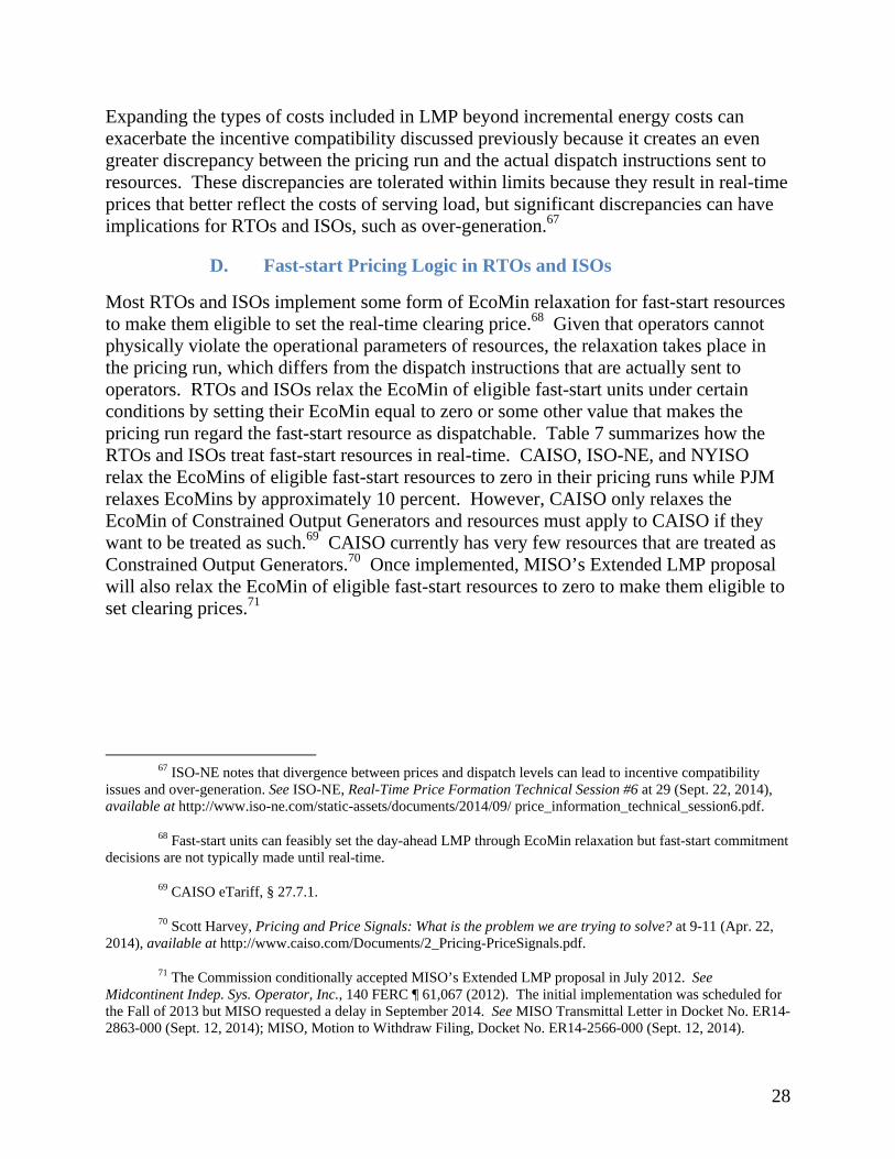
28

Expanding the types of costs included in LMP beyond incremental energy costs can exacerbate the incentive compatibility discussed previously because it creates an even greater discrepancy between the pricing run and the actual dispatch instructions sent to resources. These discrepancies are tolerated within limits because they result in real-time prices that better reflect the costs of serving load, but significant discrepancies can have implications for RTOs and ISOs, such as over-generation.67

D. Fast-start Pricing Logic in RTOs and ISOs

Most RTOs and ISOs implement some form of EcoMin relaxation for fast-start resources to make them eligible to set the real-time clearing price.68 Given that operators cannot physically violate the operational parameters of resources, the relaxation takes place in the pricing run, which differs from the dispatch instructions that are actually sent to operators. RTOs and ISOs relax the EcoMin of eligible fast-start units under certain conditions by setting their EcoMin equal to zero or some other value that makes the pricing run regard the fast-start resource as dispatchable. Table 7 summarizes how the RTOs and ISOs treat fast-start resources in real-time. CAISO, ISO-NE, and NYISO relax the EcoMins of eligible fast-start resources to zero in their pricing runs while PJM relaxes EcoMins by approximately 10 percent. However, CAISO only relaxes the EcoMin of Constrained Output Generators and resources must apply to CAISO if they want to be treated as such.69 CAISO currently has very few resources that are treated as Constrained Output Generators.70 Once implemented, MISO’s Extended LMP proposal will also relax the EcoMin of eligible fast-start resources to zero to make them eligible to set clearing prices.71

67 ISO-NE notes that divergence between prices and dispatch levels can lead to incentive compatibility

issues and over-generation. See ISO-NE, Real-Time Price Formation Technical Session #6 at 29 (Sept. 22, 2014), available at http://www.iso-ne.com/static-assets/documents/2014/09/ price_information_technical_session6.pdf.

68 Fast-start units can feasibly set the day-ahead LMP through EcoMin relaxation but fast-start commitment decisions are not typically made until real-time.

69 CAISO eTariff, § 27.7.1.

70 Scott Harvey, Pricing and Price Signals: What is the problem we are trying to solve? at 9-11 (Apr. 22, 2014), available at http://www.caiso.com/Documents/2_Pricing-PriceSignals.pdf.

71 The Commission conditionally accepted MISO’s Extended LMP proposal in July 2012. See Midcontinent Indep. Sys. Operator, Inc., 140 FERC ¶ 61,067 (2012). The initial implementation was scheduled for the Fall of 2013 but MISO requested a delay in September 2014. See MISO Transmittal Letter in Docket No. ER14-2863-000 (Sept. 12, 2014); MISO, Motion to Withdraw Filing, Docket No. ER14-2566-000 (Sept. 12, 2014).

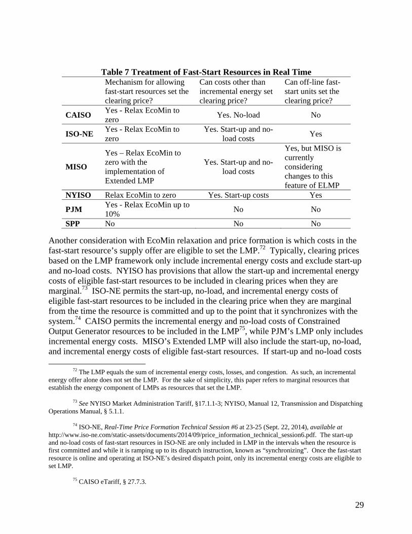
29

Table 7 Treatment of Fast-Start Resources in Real Time Mechanism for allowing

fast-start resources set the clearing price?

Can costs other than incremental energy set clearing price?

Can off-line fast-start units set the clearing price?

CAISO Yes - Relax EcoMin to zero

Yes. No-load No

ISO-NE Yes - Relax EcoMin to zero

Yes. Start-up and no-load costs

Yes

MISO

Yes – Relax EcoMin to zero with the implementation of Extended LMP

Yes. Start-up and no-load costs

Yes, but MISO is currently considering changes to this feature of ELMP

NYISO Relax EcoMin to zero Yes. Start-up costs Yes

PJM Yes - Relax EcoMin up to 10%

No No

SPP No No No

Another consideration with EcoMin relaxation and price formation is which costs in the fast-start resource’s supply offer are eligible to set the LMP.72 Typically, clearing prices based on the LMP framework only include incremental energy costs and exclude start-up and no-load costs. NYISO has provisions that allow the start-up and incremental energy costs of eligible fast-start resources to be included in clearing prices when they are marginal.73 ISO-NE permits the start-up, no-load, and incremental energy costs of eligible fast-start resources to be included in the clearing price when they are marginal from the time the resource is committed and up to the point that it synchronizes with the system.74 CAISO permits the incremental energy and no-load costs of Constrained Output Generator resources to be included in the LMP75, while PJM’s LMP only includes incremental energy costs. MISO’s Extended LMP will also include the start-up, no-load, and incremental energy costs of eligible fast-start resources. If start-up and no-load costs

72 The LMP equals the sum of incremental energy costs, losses, and congestion. As such, an incremental energy offer alone does not set the LMP. For the sake of simplicity, this paper refers to marginal resources that establish the energy component of LMPs as resources that set the LMP.

73 See NYISO Market Administration Tariff, §17.1.1-3; NYISO, Manual 12, Transmission and Dispatching Operations Manual, § 5.1.1.

74 ISO-NE, Real-Time Price Formation Technical Session #6 at 23-25 (Sept. 22, 2014), available at http://www.iso-ne.com/static-assets/documents/2014/09/price_information_technical_session6.pdf. The start-up and no-load costs of fast-start resources in ISO-NE are only included in LMP in the intervals when the resource is first committed and while it is ramping up to its dispatch instruction, known as “synchronizing”. Once the fast-start resource is online and operating at ISO-NE’s desired dispatch point, only its incremental energy costs are eligible to set LMP.

75 CAISO eTariff, § 27.7.3.

30

are included in the clearing price, they are amortized over the fast-start unit’s minimum run-time, which is typically required to be one hour or less.

Traditional real-time dispatch and pricing runs have another feature that some RTOs and ISOs have amended. Typically, the SCED that underlies the pricing run only dispatches resources that have already been committed and are thus currently online. NYISO and ISO-NE have modified their pricing run to expand the set of resources that can be dispatched in the pricing run. Both ISOs allow eligible fast-start units that are off-line to set the clearing price during the interval when the resource is starting up. As explained in section IV.B, the rationale for allowing off-line fast-start resources to set the clearing price is that it will result in prices that better reflect the cost of serving the next increment of load, which may involve committing a fast-start resource that is off-line. MISO’s original Extended LMP proposal permitted off-line fast-start resources to establish the LMP. MISO’s market monitor raised concerns about certain design elements of the Extended LMP proposal and MISO is currently developing alternative proposals to address those concerns.76

V. Empirical Analysis

The extent of the price formation issues associated with operator-initiated actions discussed above is dependent on the actual amount of capacity ISOs and RTOs are committing that are not reflected in energy and ancillary services prices. If ISOs and RTOs only commit a limited number of resources outside of the day-ahead or real-time market processes, then the issues discussed above would largely be theoretical. This section presents an empirical analysis based on data provided pursuant to Order No. 76077 and publicly available data to examine the extent to which out-of-market commitments are made in RTOs and ISOs. The data provided pursuant to Order No. 760 does not explicitly identify which commitments were initiated by operators, so this analysis takes a narrow focus and develops a conservative indicator of resource commitments that were potentially operator-initiated. This analysis found that the average MW of capacity operating at or close to EcoMin for the duration of its commitment period constituted a small portion of load. However, the analysis also found that the MW operating at EcoMin is highly variable, and can reach up to 5 percent of average load on some days.

76 MISO, Motion to Withdraw Filing, Docket No. ER14-2566-000, at 3, (Sept. 12, 2014).

77 Enhancement of Electricity Market Surveillance and Analysis through Ongoing Electronic Delivery from Regional Transmission Organizations and Independent System Operators, Order No. 760, FERC Stats. & Regs. ¶31,330 (2012). Paragraph 35 of Order No. 760 states the Commission may make publicly available staff white papers, among other things, that contain analyses derived from data that the Commission uses.

31

A. Methodology

This analysis examines the extent to which resources that were not self-scheduled, and committed and operated at a level close to their EcoMin for the duration of their commitment period. In the absence of more definitive data, this metric is a reasonable estimate of the extent to which resources are committed out-of-market by operators, either through an automated process like the RUC or through a manual commitment. As explained below, this estimate could be regarded as a lower bound estimate.

The analysis identified resources committed at or near EcoMin because market-based commitments are unlikely to commit resources to remain at EcoMin for their entire dispatch periods on a persistent basis. It is more likely that resources that are committed at their EcoMin levels and remain at that level for the duration of their commitment are committed outside of a market clearing process because, with the exception of fast-start resources, resources committed as part of the market process are dispatched at levels above their EcoMin. If a resource is inframarginal, then it is optimal to increase its dispatch as much as possible because its costs are below those of the marginal unit. Unless it is a fast-start resource with a relaxed EcoMin, the marginal unit is unlikely to be at EcoMin because, as explained in section IV.A, marginal units must be dispatchable – which implies that they are not operating at EcoMin.

This metric may over- or understate operator-initiated commitments. It may over-state operator-initiated commitments to the extent that identified resources were committed at their EcoMin by a market optimization process and not through operator actions. For example, given EcoMin relaxation, it is possible that some resources committed at EcoMin can set the clearing price. However, this measure is more likely to understate out-of-market operator-initiated commitments than it is to overstate them. First, this measure does not capture instances of operator-initiated commitments that were over 5 percent above EcoMin. Second, this estimate does not capture operator-committed resources that spend a portion of their commitment dispatched close to their EcoMin and another portion dispatched above EcoMin.78 Finally, the estimate does not capture instances when resources that were initially self-scheduled or committed on the basis of economics were asked to remain online by operators. Thus, despite these sources of imprecision, this metric is a useful and conservative indicator of the extent to which out-of-market operator-initiated commitments are present in the markets examined.

The analysis examined hourly commitment and dispatch data provided pursuant to Order No. 760 in 2013. Each non-self-scheduled commitment observed was classified as either an EcoMin commitment or a non-EcoMin commitment, based on whether the resource was dispatched close to its EcoMin for the entire duration of its daily commitment. The

78 This scenario may occur if a resource is initially committed by an operator-initiated process and

subsequently dispatched up because, once committed, its energy costs are economic.

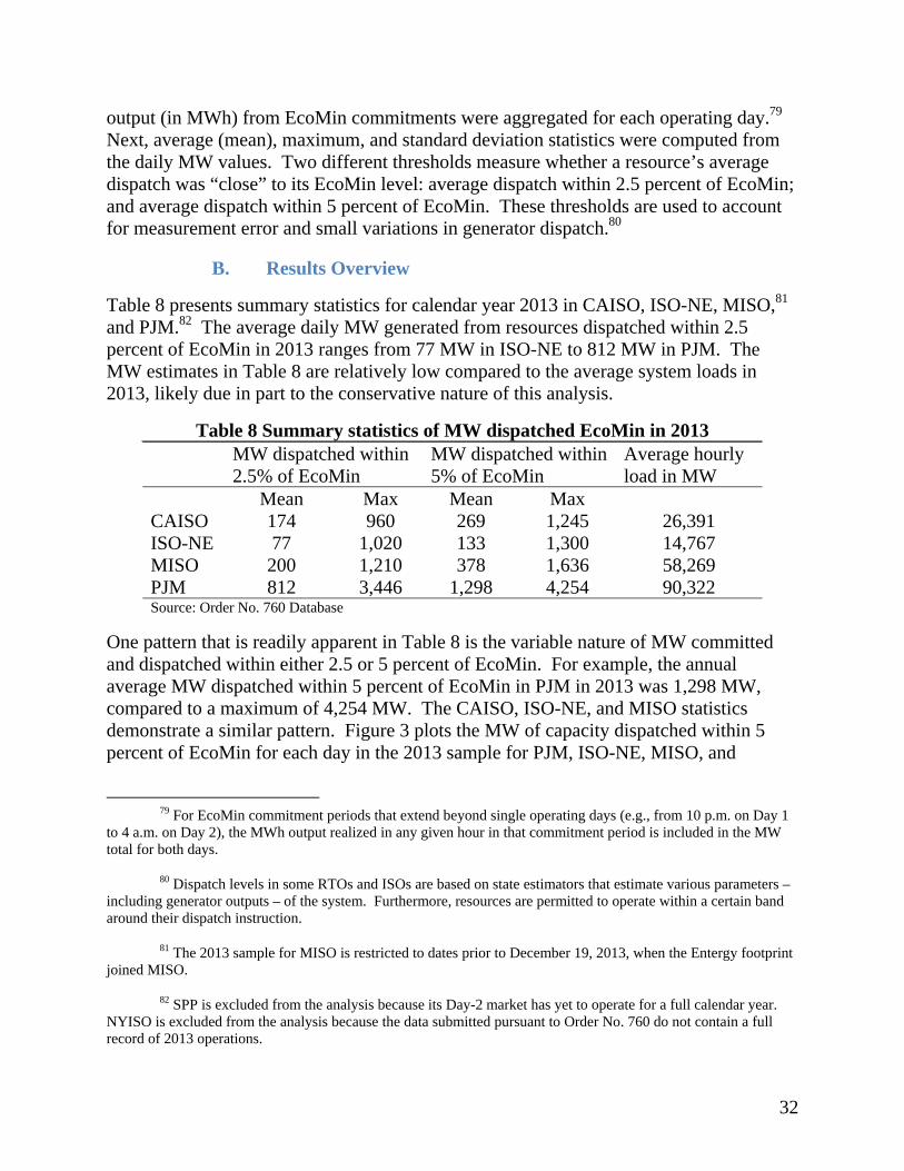
32

output (in MWh) from EcoMin commitments were aggregated for each operating day.79 Next, average (mean), maximum, and standard deviation statistics were computed from the daily MW values. Two different thresholds measure whether a resource’s average dispatch was “close” to its EcoMin level: average dispatch within 2.5 percent of EcoMin; and average dispatch within 5 percent of EcoMin. These thresholds are used to account for measurement error and small variations in generator dispatch.80

B. Results Overview

Table 8 presents summary statistics for calendar year 2013 in CAISO, ISO-NE, MISO,81 and PJM.82 The average daily MW generated from resources dispatched within 2.5 percent of EcoMin in 2013 ranges from 77 MW in ISO-NE to 812 MW in PJM. The MW estimates in Table 8 are relatively low compared to the average system loads in 2013, likely due in part to the conservative nature of this analysis.

Table 8 Summary statistics of MW dispatched EcoMin in 2013 MW dispatched within

2.5% of EcoMin MW dispatched within 5% of EcoMin

Average hourly load in MW

Mean Max Mean Max CAISO 174 960 269 1,245 26,391 ISO-NE 77 1,020 133 1,300 14,767 MISO 200 1,210 378 1,636 58,269 PJM 812 3,446 1,298 4,254 90,322 Source: Order No. 760 Database

One pattern that is readily apparent in Table 8 is the variable nature of MW committed and dispatched within either 2.5 or 5 percent of EcoMin. For example, the annual average MW dispatched within 5 percent of EcoMin in PJM in 2013 was 1,298 MW, compared to a maximum of 4,254 MW. The CAISO, ISO-NE, and MISO statistics demonstrate a similar pattern. Figure 3 plots the MW of capacity dispatched within 5 percent of EcoMin for each day in the 2013 sample for PJM, ISO-NE, MISO, and

79 For EcoMin commitment periods that extend beyond single operating days (e.g., from 10 p.m. on Day 1

to 4 a.m. on Day 2), the MWh output realized in any given hour in that commitment period is included in the MW total for both days.

80 Dispatch levels in some RTOs and ISOs are based on state estimators that estimate various parameters – including generator outputs – of the system. Furthermore, resources are permitted to operate within a certain band around their dispatch instruction.

81 The 2013 sample for MISO is restricted to dates prior to December 19, 2013, when the Entergy footprint joined MISO.

82 SPP is excluded from the analysis because its Day-2 market has yet to operate for a full calendar year. NYISO is excluded from the analysis because the data submitted pursuant to Order No. 760 do not contain a full record of 2013 operations.

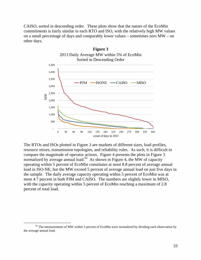
33

CAISO, sorted in descending order. These plots show that the nature of the EcoMin commitments is fairly similar in each RTO and ISO, with the relatively high MW values on a small percentage of days and comparably lower values – sometimes zero MW – on other days.

Figure 3 2013 Daily Average MW within 5% of EcoMin

Sorted in Descending Order

The RTOs and ISOs plotted in Figure 3 are markets of different sizes, load profiles, resource mixes, transmission topologies, and reliability rules. As such, it is difficult to compare the magnitude of operator actions. Figure 4 presents the plots in Figure 3 normalized by average annual load.83 As shown in Figure 4, the MW of capacity operating within 5 percent of EcoMin constitutes at most 8.8 percent of average annual load in ISO-NE, but the MW exceed 5 percent of average annual load on just five days in the sample. The daily average capacity operating within 5 percent of EcoMin was at most 4.7 percent in both PJM and CAISO. The numbers are slightly lower in MISO, with the capacity operating within 5 percent of EcoMin reaching a maximum of 2.8 percent of total load.

83 The measurements of MW within 5 percent of EcoMin were normalized by dividing each observation by

the average annual load.

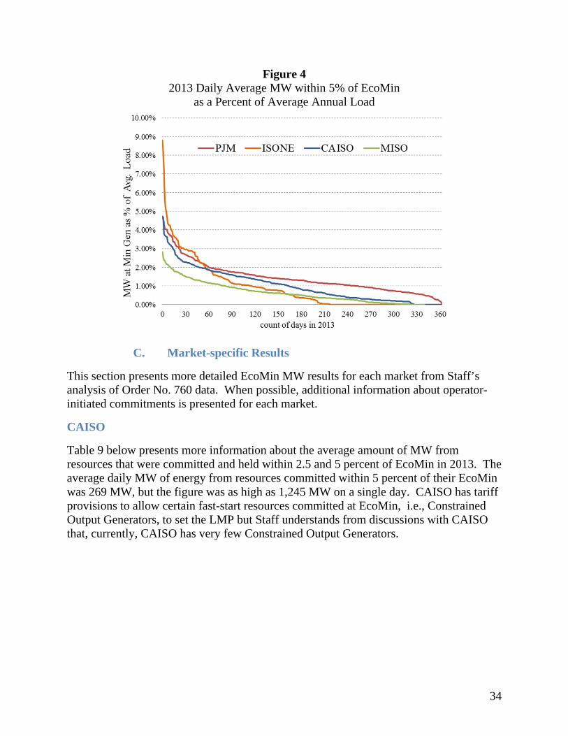
34

Figure 4 2013 Daily Average MW within 5% of EcoMin

as a Percent of Average Annual Load

C. Market-specific Results

This section presents more detailed EcoMin MW results for each market from Staff’s analysis of Order No. 760 data. When possible, additional information about operator-initiated commitments is presented for each market.

CAISO

Table 9 below presents more information about the average amount of MW from resources that were committed and held within 2.5 and 5 percent of EcoMin in 2013. The average daily MW of energy from resources committed within 5 percent of their EcoMin was 269 MW, but the figure was as high as 1,245 MW on a single day. CAISO has tariff provisions to allow certain fast-start resources committed at EcoMin, i.e., Constrained Output Generators, to set the LMP but Staff understands from discussions with CAISO that, currently, CAISO has very few Constrained Output Generators.

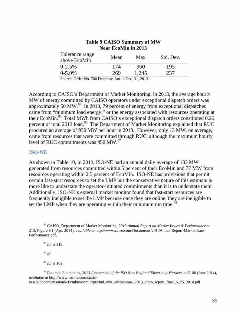
35

Table 9 CAISO Summary of MW Near EcoMin in 2013

Tolerance range above EcoMin

Mean Max Std. Dev.

0-2.5% 174 960 195 0-5.0% 269 1,245 237 Source: Order No. 760 Database, Jan. 1-Dec. 31, 2013

According to CAISO’s Department of Market Monitoring, in 2013, the average hourly MW of energy committed by CAISO operators under exceptional dispatch orders was approximately 50 MW.84 In 2013, 79 percent of energy from exceptional dispatches came from “minimum load energy,” or the energy associated with resources operating at their EcoMin.85 Total MWh from CAISO’s exceptional dispatch orders constituted 0.26 percent of total 2013 load.86 The Department of Market Monitoring explained that RUC procured an average of 930 MW per hour in 2013. However, only 13 MW, on average, came from resources that were committed through RUC, although the maximum hourly level of RUC commitments was 450 MW.87

ISO-NE

As shown in Table 10, in 2013, ISO-NE had an annual daily average of 133 MW generated from resources committed within 5 percent of their EcoMin and 77 MW from resources operating within 2.5 percent of EcoMin. ISO-NE has provisions that permit certain fast-start resources to set the LMP but the conservative nature of this estimate is more like to understate the operator-initiated commitments than it is to understate them. Additionally, ISO-NE’s external market monitor found that fast-start resources are frequently ineligible to set the LMP because once they are online, they are ineligible to set the LMP when they are operating within their minimum run time.88

84 CAISO, Department of Market Monitoring, 2013 Annual Report on Market Issues & Performance at 213, Figure 9.1 (Apr. 2014), available at http://www.caiso.com/Documents/2013AnnualReport-MarketIssue-Performance.pdf.

85 Id. at 212.

86 Id.

87 Id. at 102.

88 Potomac Economics, 2013 Assessment of the ISO New England Electricity Markets at 87-88 (June 2014), available at http://www.iso-ne.com/static-assets/documents/markets/mktmonmit/rpts/ind_mkt_advsr/isone_2013_emm_report_final_6_25_2014.pdf

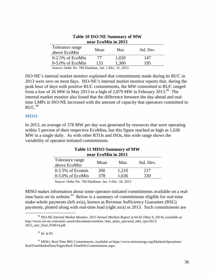
36

Table 10 ISO-NE Summary of MW near EcoMin in 2013

Tolerance range above EcoMin

Mean Max Std. Dev.

0-2.5% of EcoMin 77 1,020 147 0-5.0% of EcoMin 133 1,300 195 Source: Order No. 760 Database, Jan. 1-Dec. 31, 2013

ISO-NE’s internal market monitor explained that commitments made during its RUC in 2013 were zero on most days. ISO-NE’s internal market monitor reports that, during the peak hour of days with positive RUC commitments, the MW committed in RUC ranged from a low of 26 MW in May 2013 to a high of 2,879 MW in February 2013.89 The internal market monitor also found that the difference between the day-ahead and real-time LMPs in ISO-NE increased with the amount of capacity that operators committed in RUC.90

MISO

In 2013, an average of 378 MW per day was generated by resources that were operating within 5 percent of their respective EcoMins, but this figure reached as high as 1,636 MW in a single daily. As with other RTOs and ISOs, this wide range shows the variability of operator-initiated commitments.

Table 11 MISO Summary of MW near EcoMin in 2013

Tolerance range above EcoMin

Mean Max Std. Dev.

0-2.5% of Ecomin 200 1,210 217 0-5.0% of EcoMin 378 1,636 330 Source: Order No. 760 Database, Jan. 1-Dec. 18, 2013

MISO makes information about some operator-initiated commitments available on a real-time basis on its website.91 Below is a summary of commitments eligible for real-time make-whole payments (left axis), known as Revenue Sufficiency Guarantee (RSG) payments, plotted along with real-time load (right axis) in 2013. Such commitments are

89 ISO-NE Internal Market Monitor, 2013 Annual Markets Report at 64-65 (May 6, 2014), available at http://www.iso-ne.com/static-assets/documents/markets /mkt_anlys_rpts/annl_mkt_rpts/2013/ 2013_amr_final_050614.pdf.

90 Id. at 83.

91 MISO, Real-Time RSG Commitments, available at https://www.misoenergy.org/MarketsOperations/ RealTimeMarketData/Pages/Real-TimeRSGCommitments.aspx.

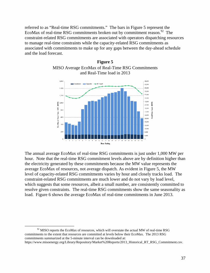
37

referred to as “Real-time RSG commitments.” The bars in Figure 5 represent the EcoMax of real-time RSG commitments broken out by commitment reason.92 The constraint-related RSG commitments are associated with operators dispatching resources to manage real-time constraints while the capacity-related RSG commitments as associated with commitments to make up for any gaps between the day-ahead schedule and the load forecast.

Figure 5 MISO Average EcoMax of Real-Time RSG Commitments

and Real-Time load in 2013

The annual average EcoMax of real-time RSG commitments is just under 1,000 MW per hour. Note that the real-time RSG commitment levels above are by definition higher than the electricity generated by these commitments because the MW value represents the average EcoMax of resources, not average dispatch. As evident in Figure 5, the MW level of capacity-related RSG commitments varies by hour and closely tracks load. The constraint-related RSG commitments are much lower and do not vary by load level, which suggests that some resources, albeit a small number, are consistently committed to resolve given constraints. The real-time RSG commitments show the same seasonality as load. Figure 6 shows the average EcoMax of real-time commitments in June 2013.

92 MISO reports the EcoMax of resources, which will overstate the actual MW of real-time RSG

commitments to the extent that resources are committed at levels below their EcoMax. The 2013 RSG commitments summarized at the 5-minute interval can be downloaded at: https://www.misoenergy.org/Library/Repository/Market%20Reports/2013_Historical_RT_RSG_Commitment.csv.

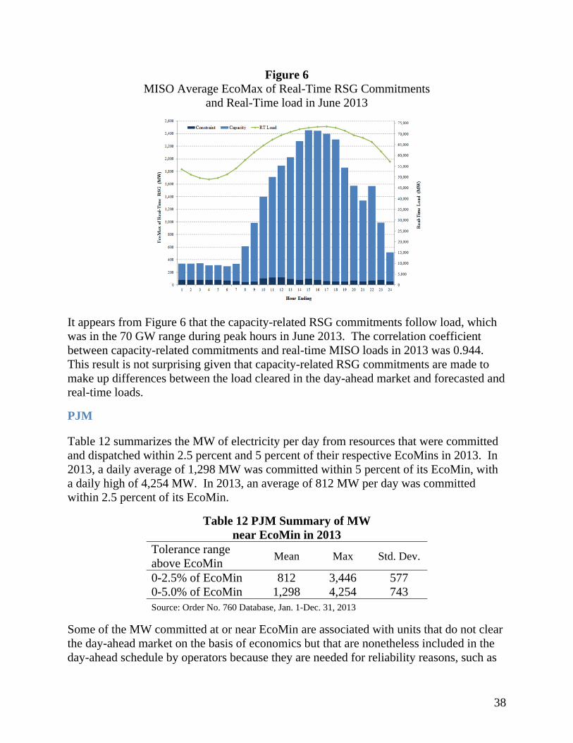
38

Figure 6 MISO Average EcoMax of Real-Time RSG Commitments

and Real-Time load in June 2013

It appears from Figure 6 that the capacity-related RSG commitments follow load, which was in the 70 GW range during peak hours in June 2013. The correlation coefficient between capacity-related commitments and real-time MISO loads in 2013 was 0.944. This result is not surprising given that capacity-related RSG commitments are made to make up differences between the load cleared in the day-ahead market and forecasted and real-time loads.

PJM

Table 12 summarizes the MW of electricity per day from resources that were committed and dispatched within 2.5 percent and 5 percent of their respective EcoMins in 2013. In 2013, a daily average of 1,298 MW was committed within 5 percent of its EcoMin, with a daily high of 4,254 MW. In 2013, an average of 812 MW per day was committed within 2.5 percent of its EcoMin.

Table 12 PJM Summary of MW near EcoMin in 2013

Tolerance range above EcoMin

Mean Max Std. Dev.

0-2.5% of EcoMin 812 3,446 577 0-5.0% of EcoMin 1,298 4,254 743 Source: Order No. 760 Database, Jan. 1-Dec. 31, 2013

Some of the MW committed at or near EcoMin are associated with units that do not clear the day-ahead market on the basis of economics but that are nonetheless included in the day-ahead schedule by operators because they are needed for reliability reasons, such as

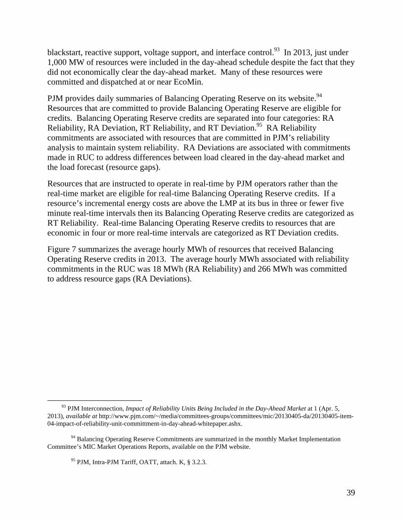
39

blackstart, reactive support, voltage support, and interface control.93 In 2013, just under 1,000 MW of resources were included in the day-ahead schedule despite the fact that they did not economically clear the day-ahead market. Many of these resources were committed and dispatched at or near EcoMin.

PJM provides daily summaries of Balancing Operating Reserve on its website.94 Resources that are committed to provide Balancing Operating Reserve are eligible for credits. Balancing Operating Reserve credits are separated into four categories: RA Reliability, RA Deviation, RT Reliability, and RT Deviation.95 RA Reliability commitments are associated with resources that are committed in PJM’s reliability analysis to maintain system reliability. RA Deviations are associated with commitments made in RUC to address differences between load cleared in the day-ahead market and the load forecast (resource gaps).

Resources that are instructed to operate in real-time by PJM operators rather than the real-time market are eligible for real-time Balancing Operating Reserve credits. If a resource’s incremental energy costs are above the LMP at its bus in three or fewer five minute real-time intervals then its Balancing Operating Reserve credits are categorized as RT Reliability. Real-time Balancing Operating Reserve credits to resources that are economic in four or more real-time intervals are categorized as RT Deviation credits.

Figure 7 summarizes the average hourly MWh of resources that received Balancing Operating Reserve credits in 2013. The average hourly MWh associated with reliability commitments in the RUC was 18 MWh (RA Reliability) and 266 MWh was committed to address resource gaps (RA Deviations).

93 PJM Interconnection, Impact of Reliability Units Being Included in the Day-Ahead Market at 1 (Apr. 5,

2013), available at http://www.pjm.com/~/media/committees-groups/committees/mic/20130405-da/20130405-item-04-impact-of-reliability-unit-committment-in-day-ahead-whitepaper.ashx. 

94 Balancing Operating Reserve Commitments are summarized in the monthly Market Implementation Committee’s MIC Market Operations Reports, available on the PJM website.

95 PJM, Intra-PJM Tariff, OATT, attach. K, § 3.2.3.

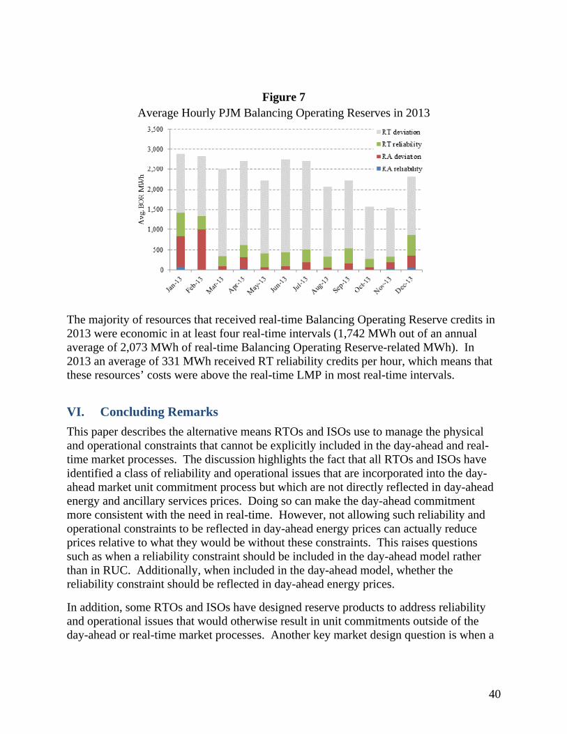
40

Figure 7 Average Hourly PJM Balancing Operating Reserves in 2013

The majority of resources that received real-time Balancing Operating Reserve credits in 2013 were economic in at least four real-time intervals (1,742 MWh out of an annual average of 2,073 MWh of real-time Balancing Operating Reserve-related MWh). In 2013 an average of 331 MWh received RT reliability credits per hour, which means that these resources’ costs were above the real-time LMP in most real-time intervals.

VI. Concluding Remarks

This paper describes the alternative means RTOs and ISOs use to manage the physical and operational constraints that cannot be explicitly included in the day-ahead and real-time market processes. The discussion highlights the fact that all RTOs and ISOs have identified a class of reliability and operational issues that are incorporated into the day-ahead market unit commitment process but which are not directly reflected in day-ahead energy and ancillary services prices. Doing so can make the day-ahead commitment more consistent with the need in real-time. However, not allowing such reliability and operational constraints to be reflected in day-ahead energy prices can actually reduce prices relative to what they would be without these constraints. This raises questions such as when a reliability constraint should be included in the day-ahead model rather than in RUC. Additionally, when included in the day-ahead model, whether the reliability constraint should be reflected in day-ahead energy prices.

In addition, some RTOs and ISOs have designed reserve products to address reliability and operational issues that would otherwise result in unit commitments outside of the day-ahead or real-time market processes. Another key market design question is when a

41

commitment that has traditionally been part of the RUC can be converted into a reserve product.

The importance of price formation concerns associated with operator-initiated actions are difficult to assess because one cannot observe what prices would have been absent the action without conducting a costly parallel market solution without the operator actions. This paper attempts to understand the degree to which resources are committed and not reflected in price by measuring the generation from capacity that was committed but not dispatched above 2.5 percent and 5 percent of their minimum operating levels. The analysis suggests that this quantity is moderate in most RTOs and ISOs but can reach fairly high levels on some days.

Finally, with regard to whether resources are fully compensated for the variable cost of providing service, this paper notes most RTOs and ISOs have some method to allow fast-start resources to set the clearing price, though the method used and the resources eligible to set price differ by market. In addition, some RTOs and ISOs allow some of a fast-start resource’s commitment costs to be reflected in energy and ancillary services prices, though the costs included differ by market. The differences across RTOs and ISOs raise the question of whether these differences are the result of differences in system needs or differences in pricing philosophy.