preprocessing techniques - mcmaster universitycs777/presentations/preprocessing.pdfxin huang ,...
TRANSCRIPT
Preprocessing Techniques
Nael El ShawwaOlesya PeshkoAlberto Olvera
Jonathan Li
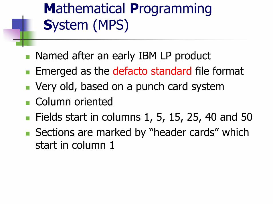
Mathematical Programming System (MPS)
Named after an early IBM LP productEmerged as the defacto standard file formatVery old, based on a punch card systemColumn orientedFields start in columns 1, 5, 15, 25, 40 and 50Sections are marked by “header cards” which start in column 1
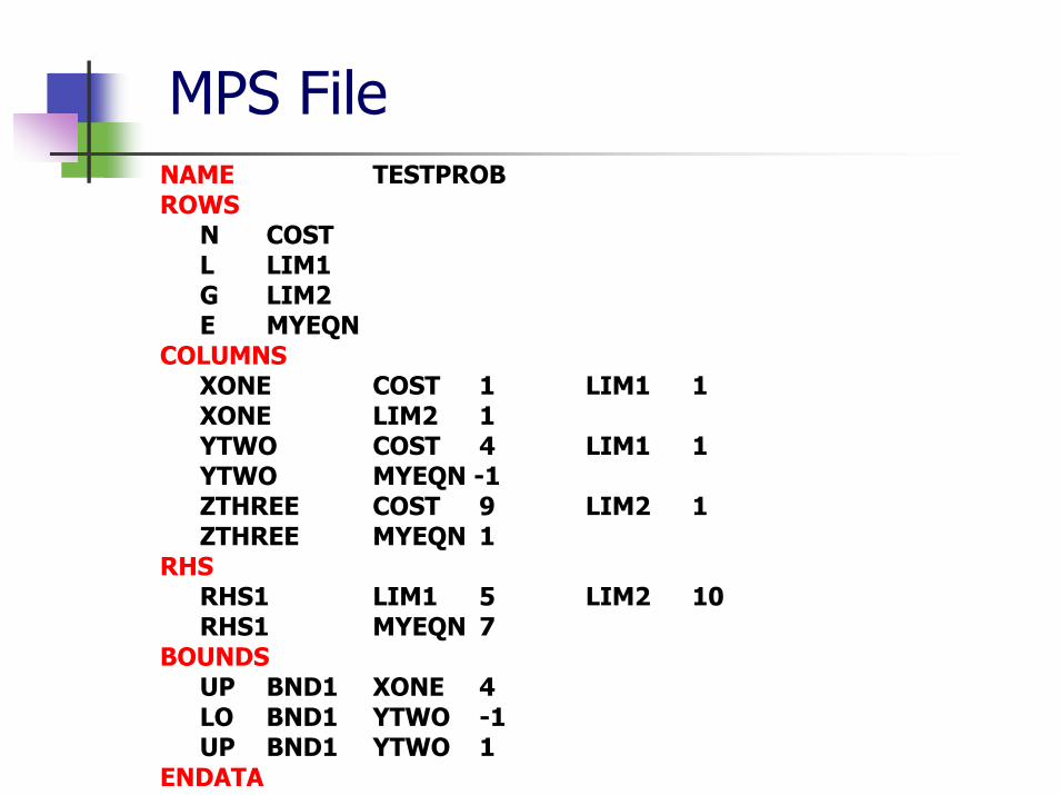
MPS FileNAME TESTPROB ROWS
N COST L LIM1 G LIM2 E MYEQN
COLUMNS XONE COST 1 LIM1 1 XONE LIM2 1 YTWO COST 4 LIM1 1 YTWO MYEQN -1 ZTHREE COST 9 LIM2 1 ZTHREE MYEQN 1
RHSRHS1 LIM1 5 LIM2 10 RHS1 MYEQN 7
BOUNDSUP BND1 XONE 4 LO BND1 YTWO -1 UP BND1 YTWO 1
ENDATA
MPS Format
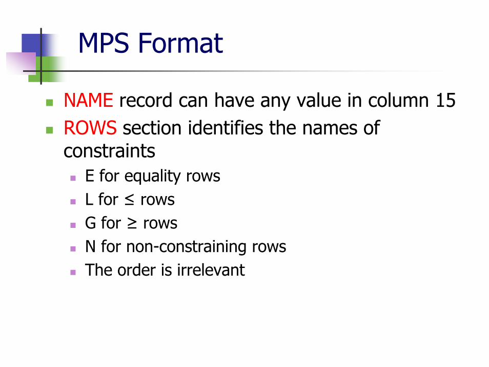
NAME record can have any value in column 15ROWS section identifies the names of constraints
E for equality rowsL for ≤ rowsG for ≥ rowsN for non-constraining rowsThe order is irrelevant
MPS Format
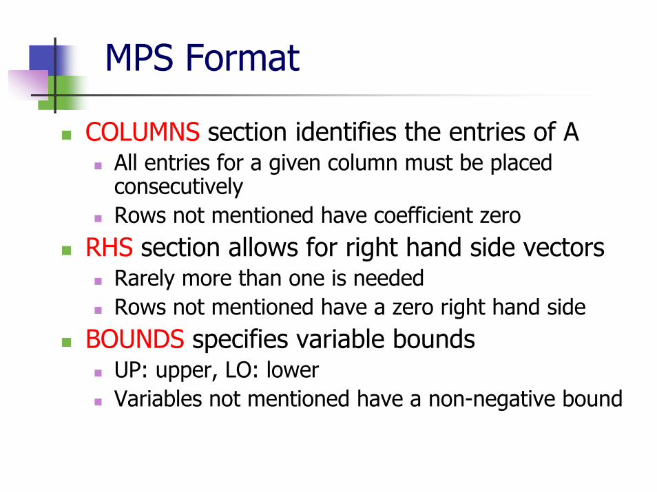
COLUMNS section identifies the entries of AAll entries for a given column must be placed consecutivelyRows not mentioned have coefficient zero
RHS section allows for right hand side vectorsRarely more than one is neededRows not mentioned have a zero right hand side
BOUNDS specifies variable boundsUP: upper, LO: lowerVariables not mentioned have a non-negative bound
From MPS to Equations
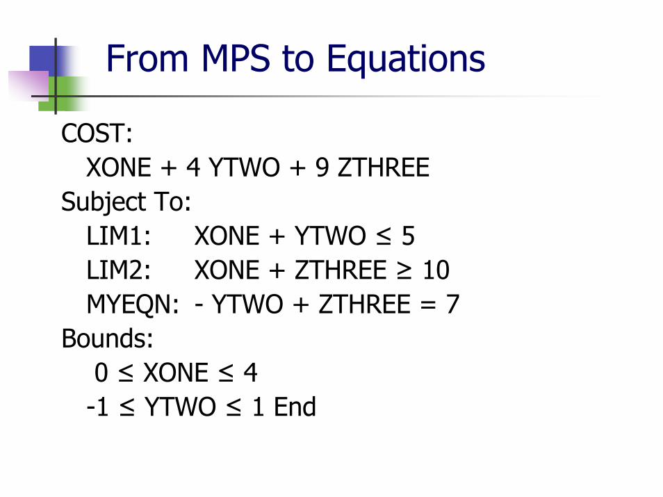
COST: XONE + 4 YTWO + 9 ZTHREE
Subject To: LIM1: XONE + YTWO ≤ 5 LIM2: XONE + ZTHREE ≥ 10 MYEQN: - YTWO + ZTHREE = 7
Bounds: 0 ≤ XONE ≤ 4 -1 ≤ YTWO ≤ 1 End

MPS FileNAME TESTPROB ROWS
N COST L LIM1 G LIM2 E MYEQN
COLUMNS XONE COST 1 LIM1 1 XONE LIM2 1 YTWO COST 4 LIM1 1 YTWO MYEQN -1 ZTHREE COST 9 LIM2 1 ZTHREE MYEQN 1
RHSRHS1 LIM1 5 LIM2 10 RHS1 MYEQN 7
BOUNDSUP BND1 XONE 4 LO BND1 YTWO -1 UP BND1 YTWO 1
ENDATA
What is preprocessing?
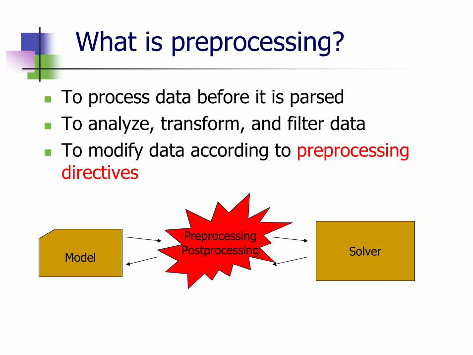
To process data before it is parsedTo analyze, transform, and filter dataTo modify data according to preprocessing directives
Model
PreprocessingPostprocessing Solver
Why should it be done?
To simplify the problem, reduce sizeEliminate redundancy in variables/constraintsSatisfy solver limitations To avoid possible numerical pitfalls and improve numerical characteristicsAims to speed up solution and efficiency
Optimization in Preprocessing
“More extensive preprocessing does not necessarily imply faster overall solution
time. Since some preprocessing techniques are quite time consuming, we have to
balance the effect of the removed redundancies with the time spent in preprocessing”
Xin Huang , Preprocessing and Post-processing in Linear Optimization, M.Sc. Thesis McMaster University, June 2004
Optimization in Preprocessing
Hard to find the best balance between effects of preprocessing and time spent preprocessing
In practice only fast techniques are chosenExpensive techniques are frequently used as tools in very large scale problems
Who does it?
The solver?Hidden heuristics the modeling system is unaware of - possible pitfalls?Solver can take advantage of certain information
The modeling system?It is the modeling systems job to filter model data for the solver, the solver just solves it
My opinion…
Not everyone uses a modeling systemSome just pass data files to solvers
Everybody uses a solverThrough a modeling system or the solver interface
The solver developers know more about their own heuristics than the modeling system developers…
How can it be justified that preprocessing is the modeling system’s job?
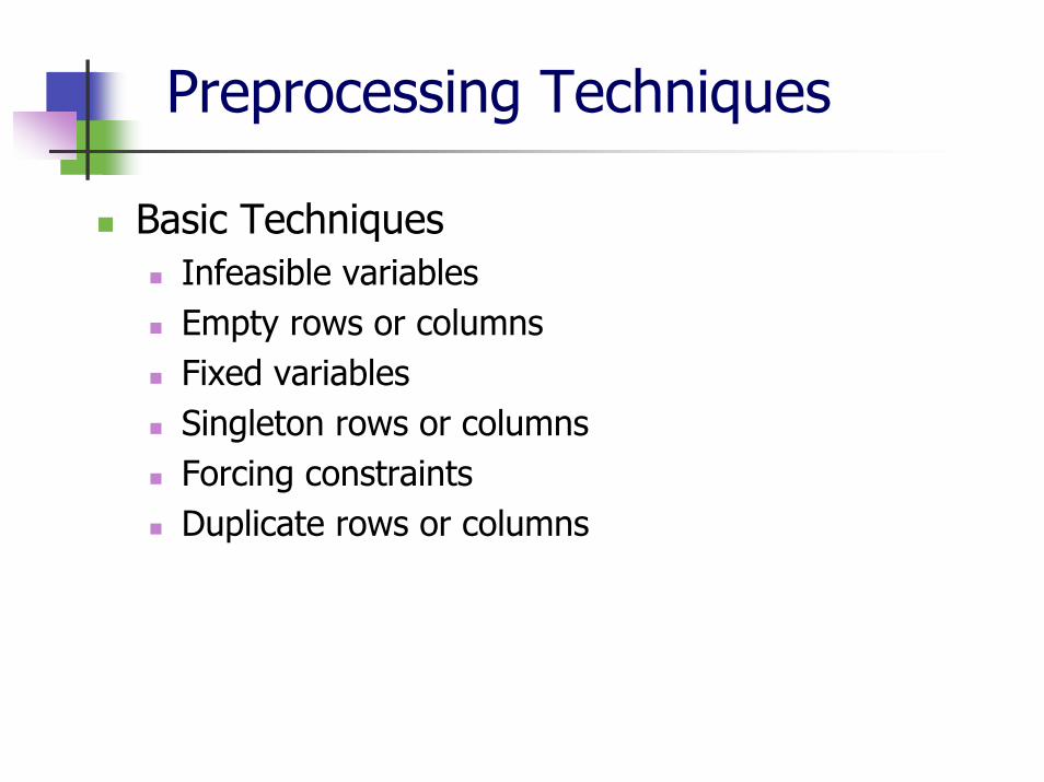
Preprocessing Techniques
Basic TechniquesInfeasible variablesEmpty rows or columnsFixed variablesSingleton rows or columnsForcing constraintsDuplicate rows or columns
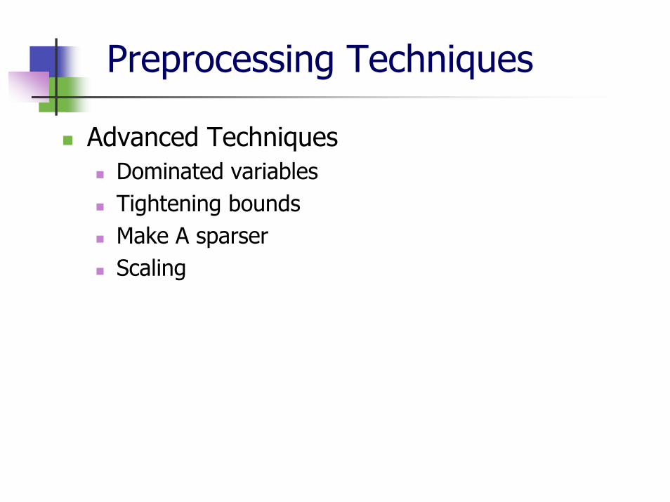
Preprocessing Techniques
Advanced TechniquesDominated variablesTightening boundsMake A sparserScaling

Basic Preprocessing Techniques
Olesya Peshko
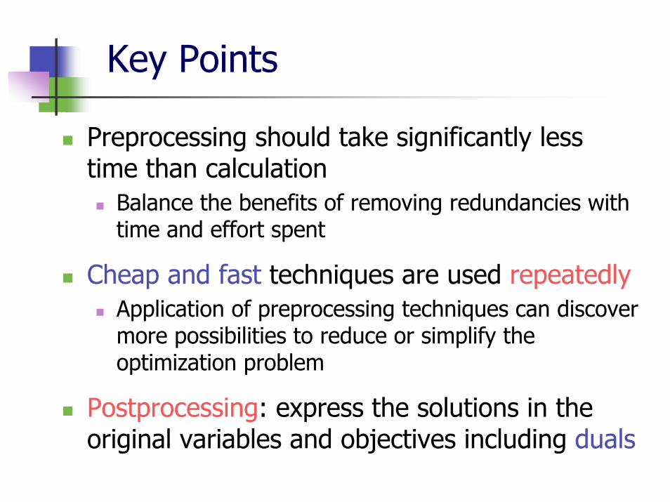
Key Points
Preprocessing should take significantly less time than calculation
Balance the benefits of removing redundancies with time and effort spent
Cheap and fast techniques are used repeatedlyApplication of preprocessing techniques can discover more possibilities to reduce or simplify the optimization problem
Postprocessing: express the solutions in the original variables and objectives including duals
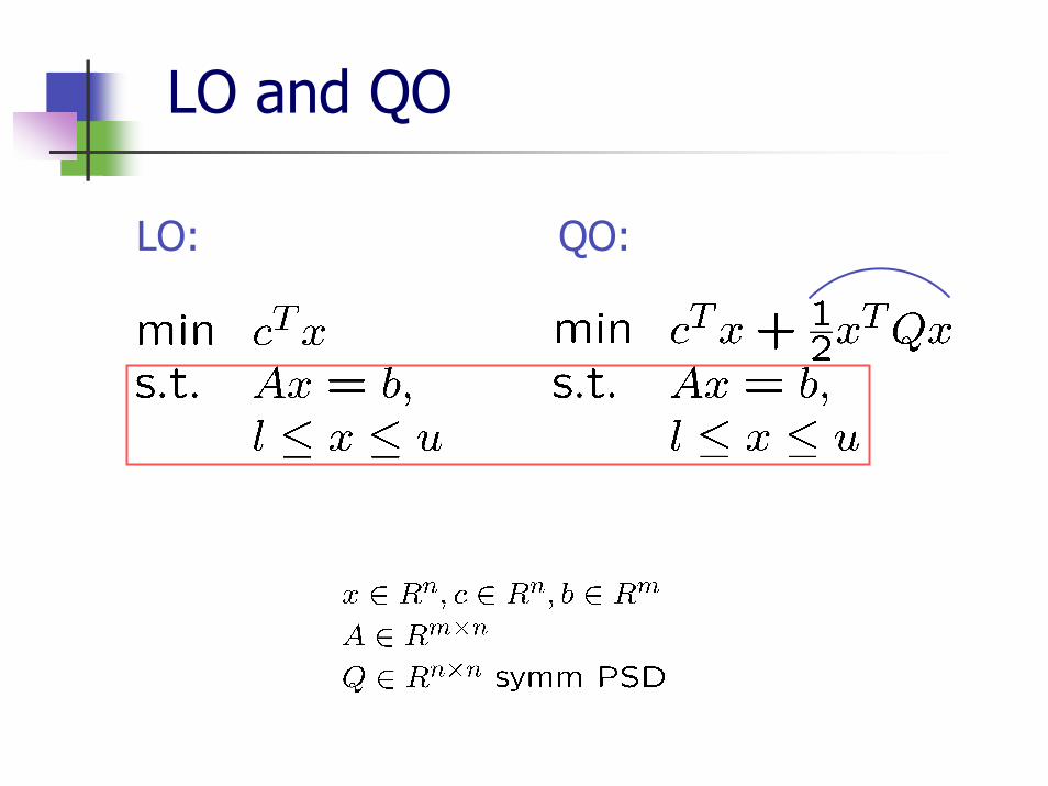
LO: QO:
LO and QO
Basic Preprocessing
For the basic preprocessing techniques the following will be discussed:
Definition
Detection
Consequences and influence on the optimization problem and solution
Results or next steps
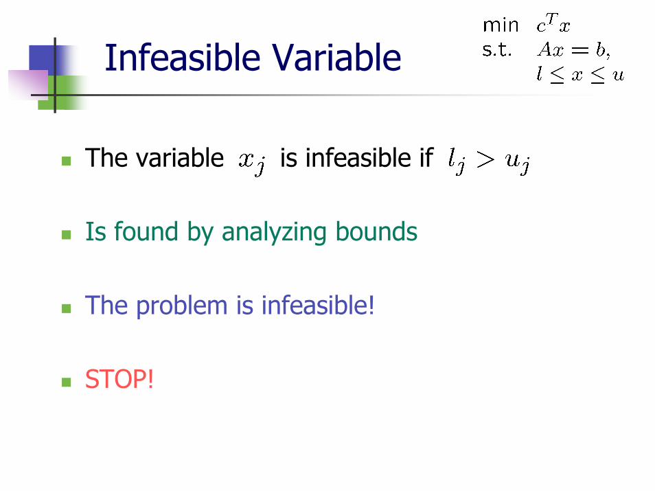
Infeasible Variable
The variable is infeasible if
Is found by analyzing bounds
The problem is infeasible!
STOP!
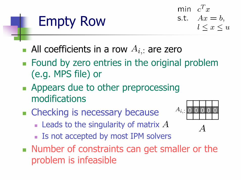
Empty Row
All coefficients in a row are zeroFound by zero entries in the original problem (e.g. MPS file) orAppears due to other preprocessing modificationsChecking is necessary because
Leads to the singularity of matrix Is not accepted by most IPM solvers
Number of constraints can get smaller or the problem is infeasible
0 0 0 0 0
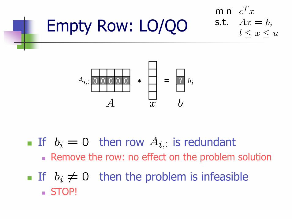
Empty Row: LO/QO
If then row is redundantRemove the row: no effect on the problem solution
If then the problem is infeasibleSTOP!
* =0 0 0 0 0 ?
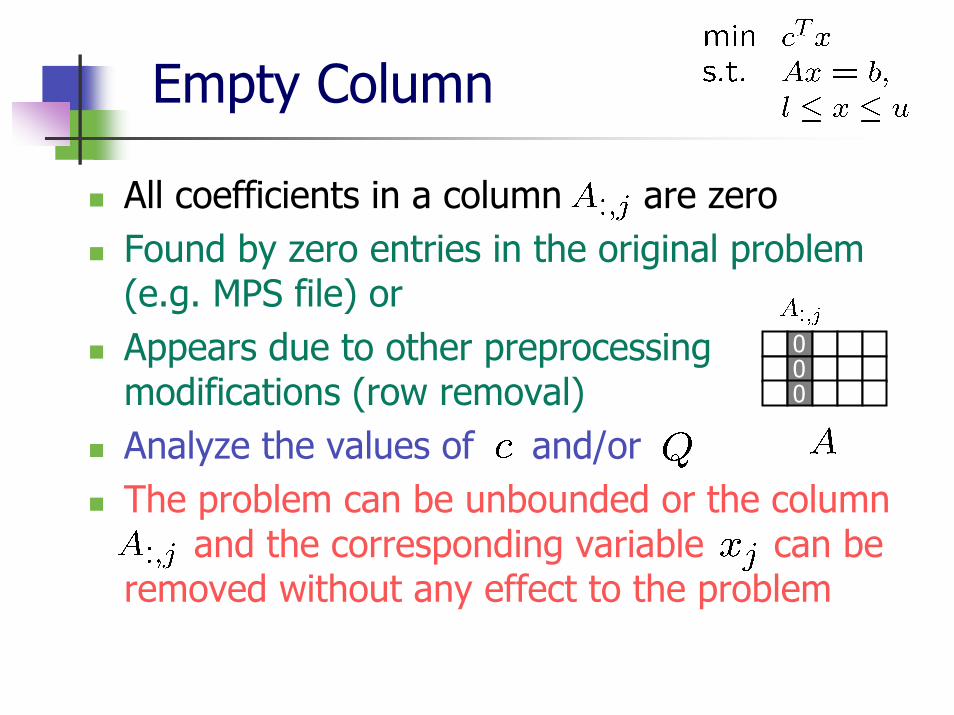
Empty Column
All coefficients in a column are zeroFound by zero entries in the original problem (e.g. MPS file) orAppears due to other preprocessing modifications (row removal)Analyze the values of and/orThe problem can be unbounded or the column
and the corresponding variable can be removed without any effect to the problem
000
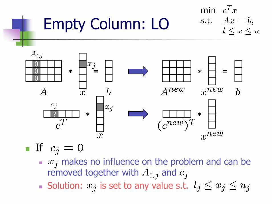
Empty Column: LO
If makes no influence on the problem and can be
removed together with and Solution: is set to any value s.t.
* =* =000
?
* *?
Empty Column: LO
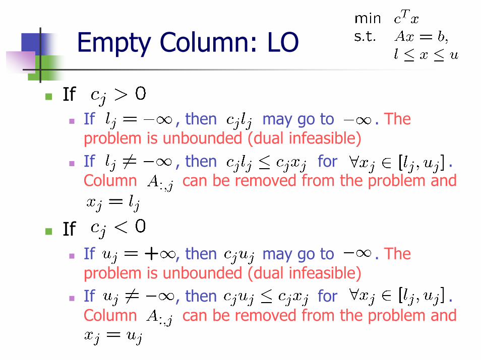
If If , then may go to . The problem is unbounded (dual infeasible)If , then for .Column can be removed from the problem and
If If , then may go to . The problem is unbounded (dual infeasible)If , then for .Column can be removed from the problem and
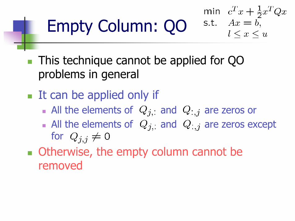
Empty Column: QO
This technique cannot be applied for QO problems in general
It can be applied only if All the elements of and are zeros orAll the elements of and are zeros except for
Otherwise, the empty column cannot be removed
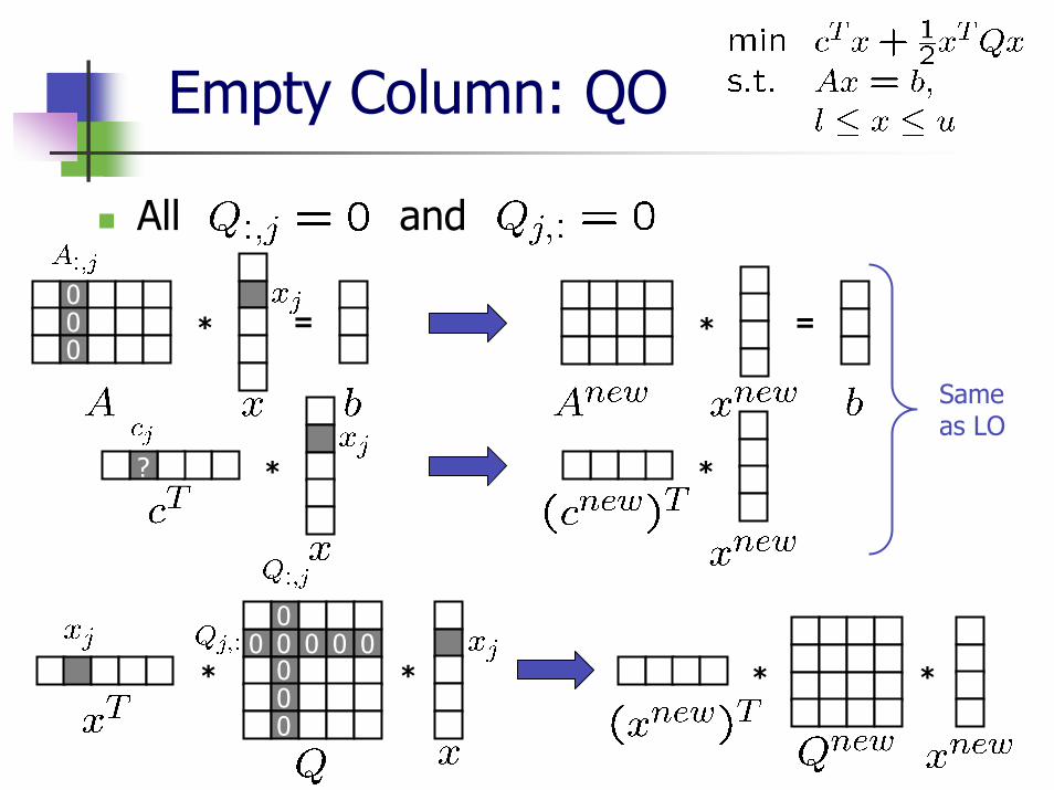
Empty Column: QO
All and
* =* =000
****
00000
0 0 0 0
Same as LO
* *?
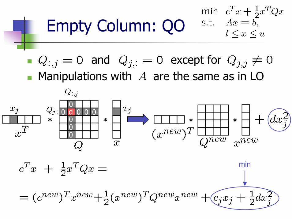
Empty Column: QO
and except for Manipulations with are the same as in LO
****
0d000
0 0 0 0
min
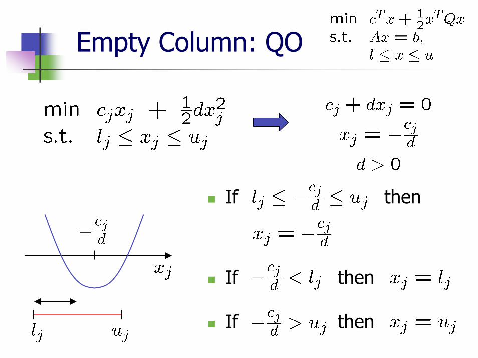
Empty Column: QO
If then
If then
If then
The variable is fixed if
Can appear in model or MPS file, section BOUNDS: variable with type definition “FX” or
Be a result of other preprocessing manipulations
The variable can be substituted by ( )
Problem size gets smaller
Fixed Variable
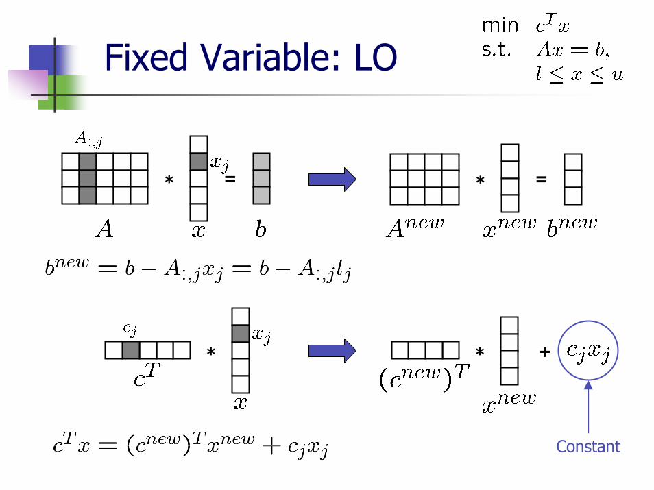
Fixed Variable: LO
* = * =
* * +
Constant
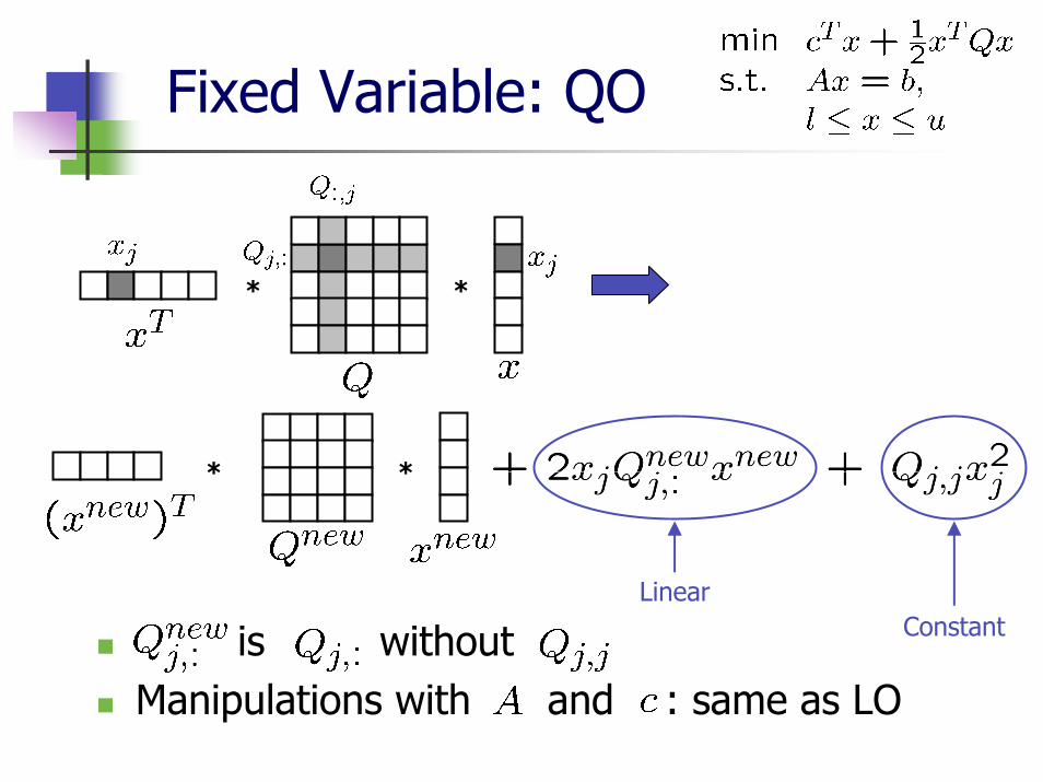
Fixed Variable: QO
is withoutManipulations with and : same as LO
**
**
ConstantLinear
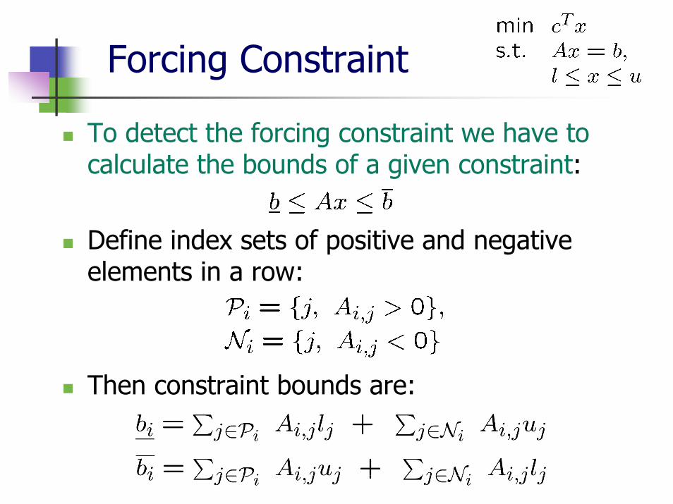
Forcing Constraint
To detect the forcing constraint we have to calculate the bounds of a given constraint:
Define index sets of positive and negative elements in a row:
Then constraint bounds are:
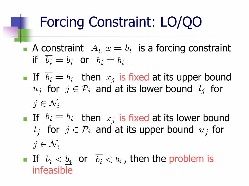
Forcing Constraint: LO/QO
A constraint is a forcing constraint if or
If then is fixed at its upper boundfor and at its lower bound for
If then is fixed at its lower boundfor and at its upper bound for
If or , then the problem is infeasible
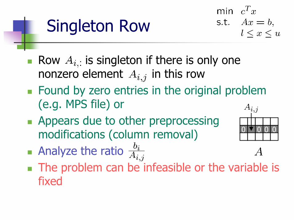
Singleton Row
Row is singleton if there is only one nonzero element in this rowFound by zero entries in the original problem (e.g. MPS file) orAppears due to other preprocessing modifications (column removal)Analyze the ratio The problem can be infeasible or the variable is fixed
0 0 0 0
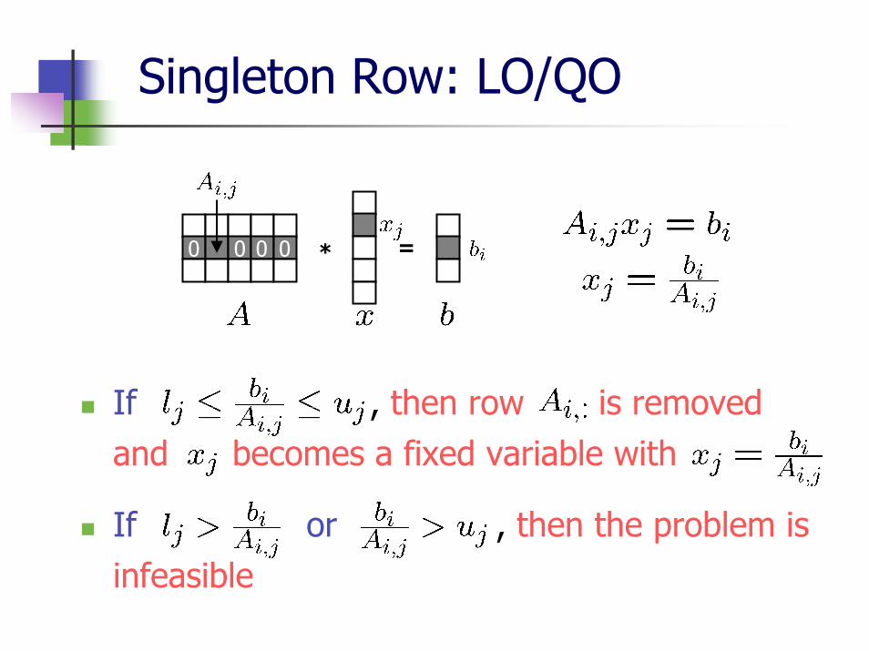
If , then row is removed and becomes a fixed variable with
If or , then the problem is infeasible
Singleton Row: LO/QO
* =0 0 0 0
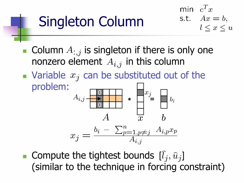
Singleton Column
Column is singleton if there is only one nonzero element in this columnVariable can be substituted out of the problem:
Compute the tightest bounds (similar to the technique in forcing constraint)
* =0
0
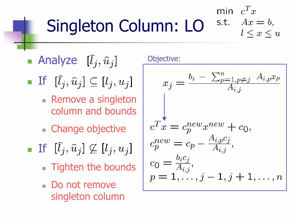
Singleton Column: LO
Analyze
If
Remove a singleton column and bounds
Change objective
If
Tighten the bounds
Do not remove singleton column
Objective:
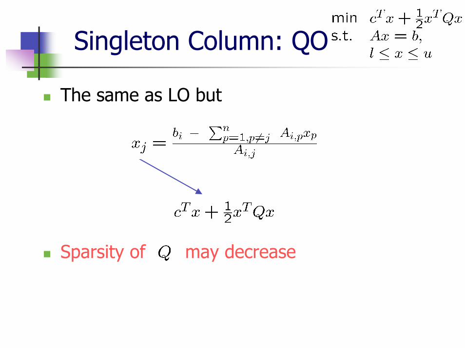
Singleton Column: QO
The same as LO but
Sparsity of may decrease
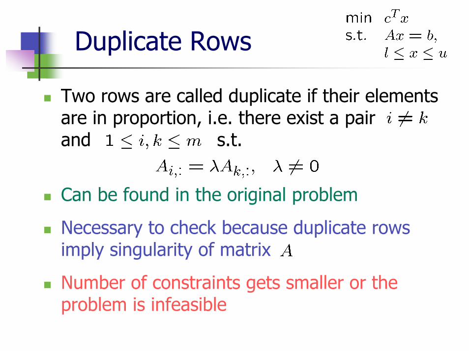
Duplicate Rows
Two rows are called duplicate if their elements are in proportion, i.e. there exist a pair and s.t.
Can be found in the original problem
Necessary to check because duplicate rows imply singularity of matrix
Number of constraints gets smaller or the problem is infeasible
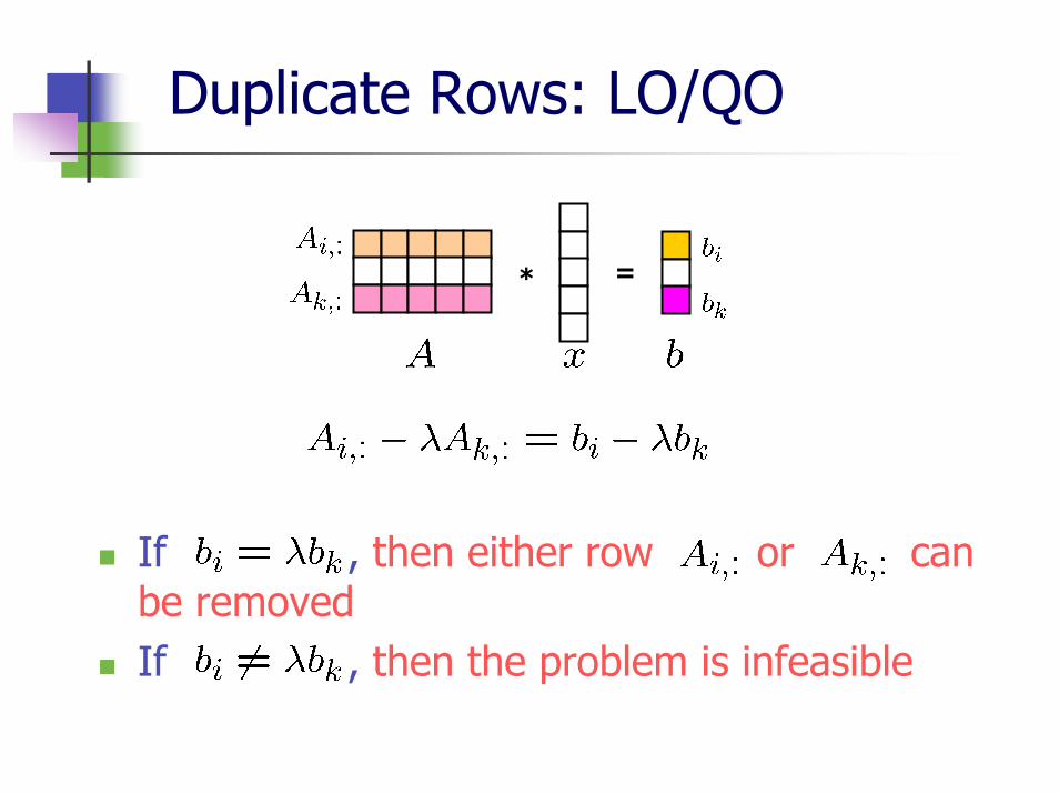
Duplicate Rows: LO/QO
If , then either row or can be removedIf , then the problem is infeasible
* =
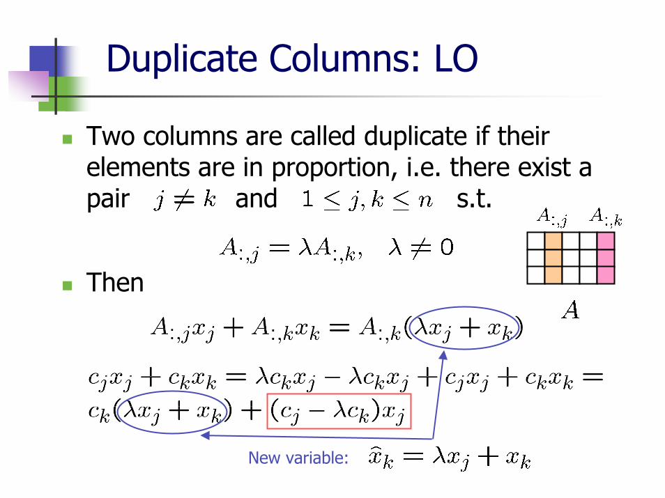
Duplicate Columns: LO
Two columns are called duplicate if their elements are in proportion, i.e. there exist a pair and s.t.
Then
New variable:
Duplicate Columns: LO
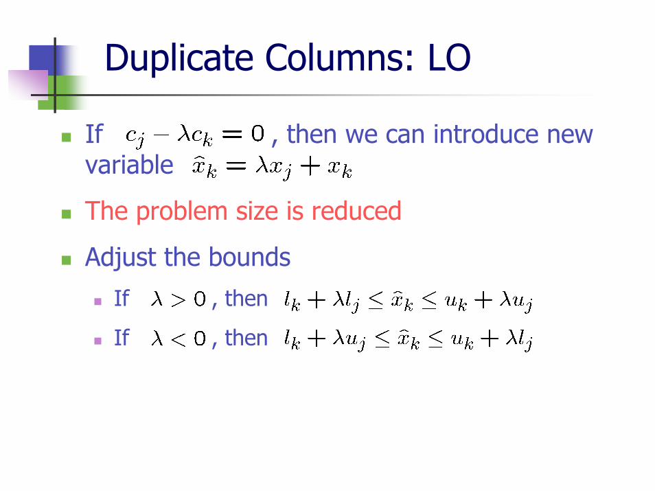
If , then we can introduce new variable
The problem size is reduced
Adjust the bounds
If , then
If , then
Duplicate Columns: LO
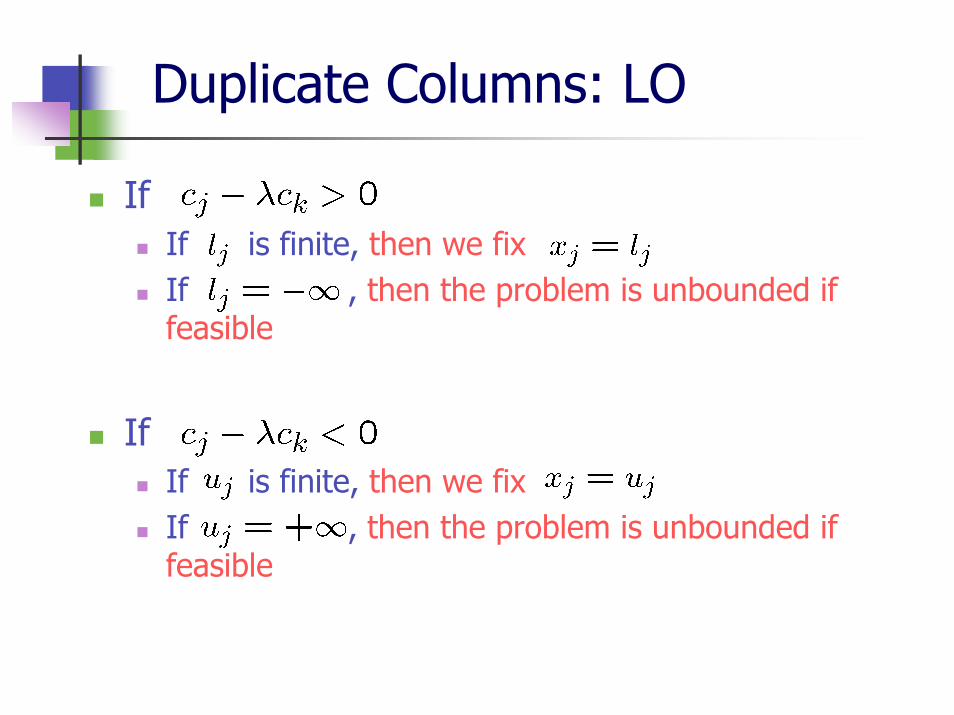
IfIf is finite, then we fix If , then the problem is unbounded if feasible
IfIf is finite, then we fix If , then the problem is unbounded if feasible
Advanced Preprocessing Techniques
Nael El Shawwa
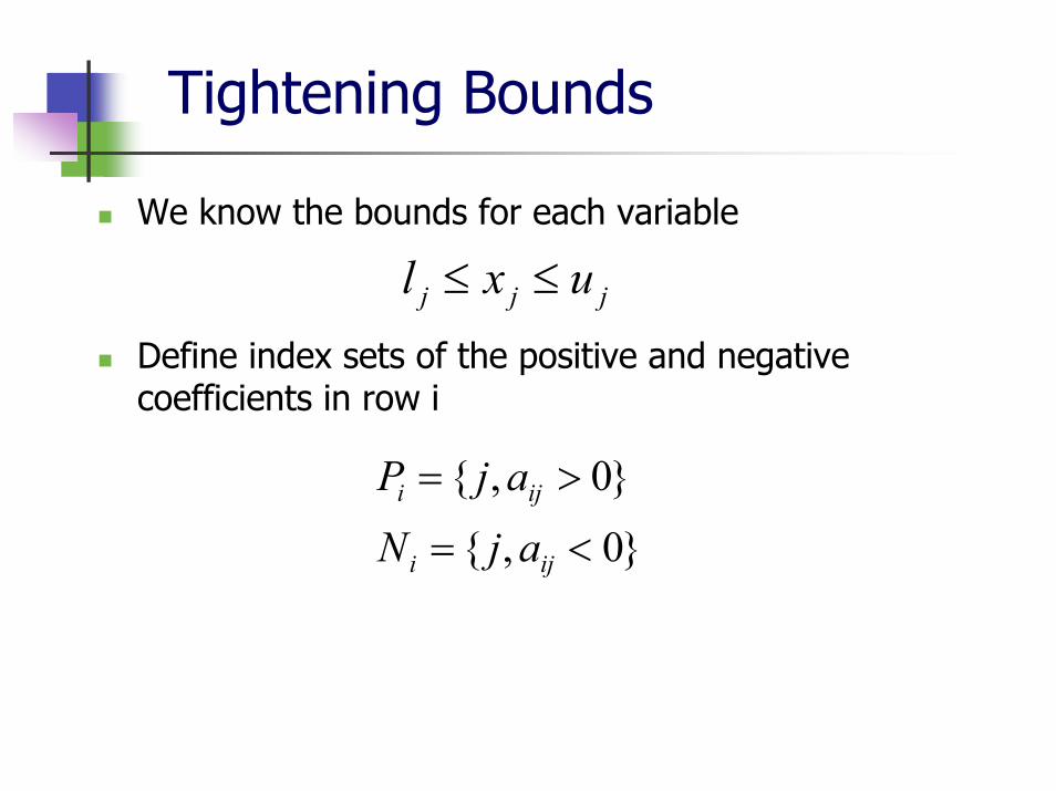
Tightening Bounds
We know the bounds for each variable
Define index sets of the positive and negative coefficients in row i
jjj uxl ≤≤
}0,{
}0,{
<=
>=
iji
iji
ajN
ajP
Tightening Bounds
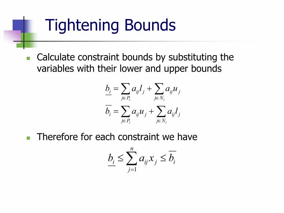
Calculate constraint bounds by substituting the variables with their lower and upper bounds
Therefore for each constraint we have
∑ ∑
∑ ∑
∈ ∈
∈ ∈
+=
+=
i i
i i
Pj Njjijjiji
Pj Njjijjiji
lauab
ualab
∑=
≤≤n
jijiji bxab
1
Tightening Bounds
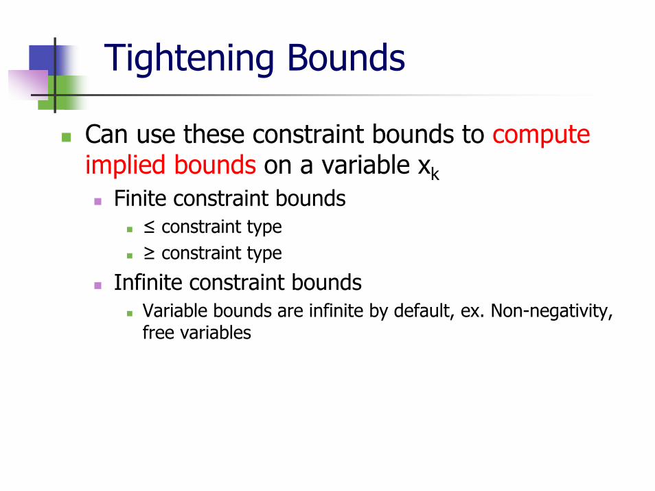
Can use these constraint bounds to compute implied bounds on a variable xk
Finite constraint bounds≤ constraint type≥ constraint type
Infinite constraint boundsVariable bounds are infinite by default, ex. Non-negativity, free variables
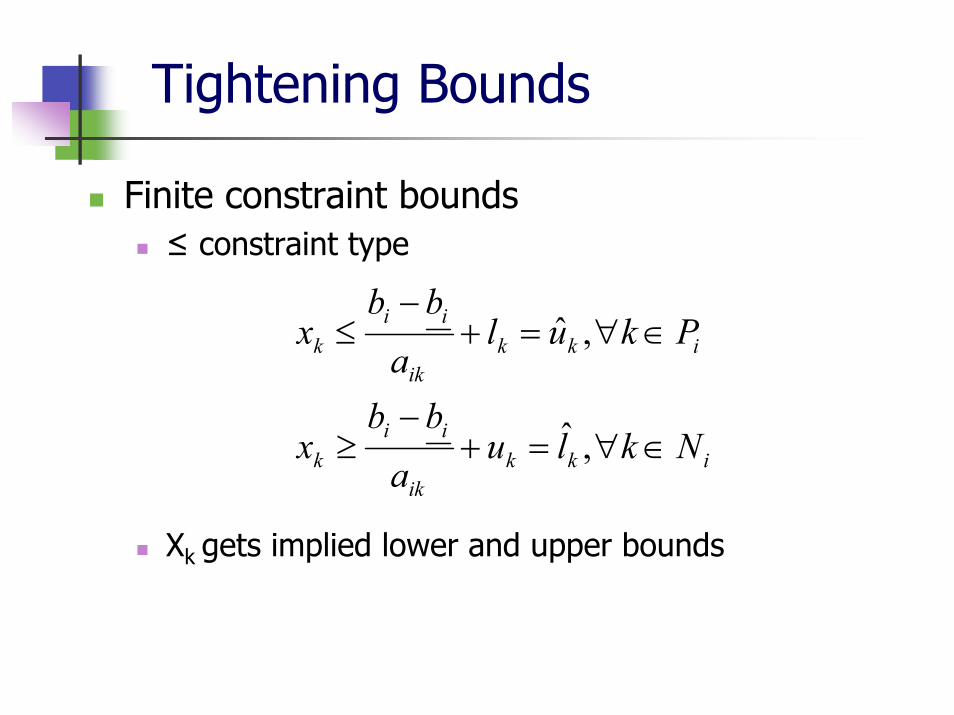
Tightening Bounds
Finite constraint bounds≤ constraint type
Xk gets implied lower and upper bounds
ikkik
iik
ikkik
iik
Nklua
bbx
Pkula
bbx
∈∀=+−
≥
∈∀=+−
≤
,ˆ
,ˆ

Tightening Bounds
Finite constraint bounds≥ constraint type
Xk gets implied lower and upper bounds
ikkik
iik
ikkik
iik
Nkula
bbx
Pklua
bbx
∈∀=+−
≤
∈∀=+−
≥
,ˆ
,ˆ
Tightening Bounds
Compare the new implied bounds with the original bounds
If they conflict then the problem is infeasibleIf they are tighter, then update the boundsIf they are looser, then maintain the bounds
What about infinite bounds?J. Gondzio, Presolve analysis of linear programs prior to applying the interior point method, INFORMS Journal on Computing 9, No. 1 (1997) pp. 73-91.Xin Huang , Preprocessing and Post-processing in Linear Optimization, M.Sc. Thesis McMaster University, June 2004
Tightening Bounds
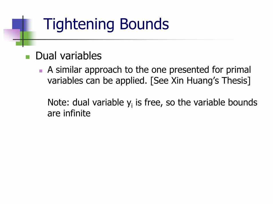
Dual variablesA similar approach to the one presented for primal variables can be applied. [See Xin Huang’s Thesis]
Note: dual variable yi is free, so the variable bounds are infinite
Dominated Variable
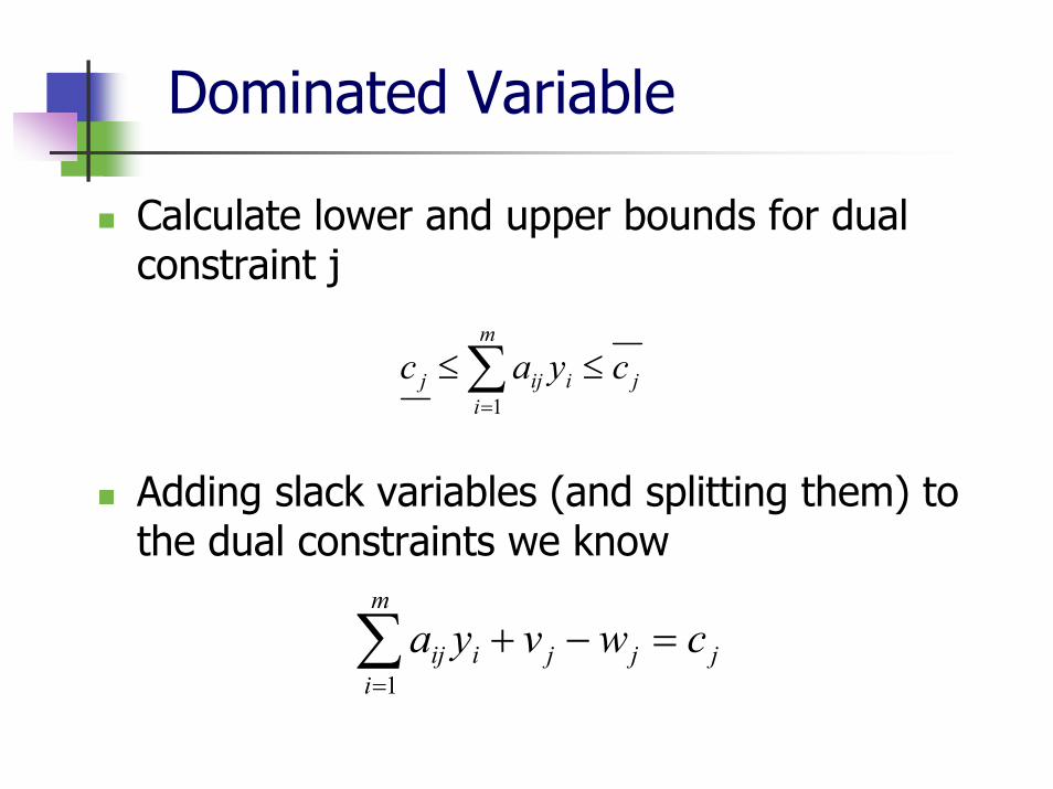
Calculate lower and upper bounds for dual constraint j
Adding slack variables (and splitting them) to the dual constraints we know
∑=
≤≤m
ijiijj cyac
1
∑=
=−+m
ijjjiij cwvya
1
Dominated Variable
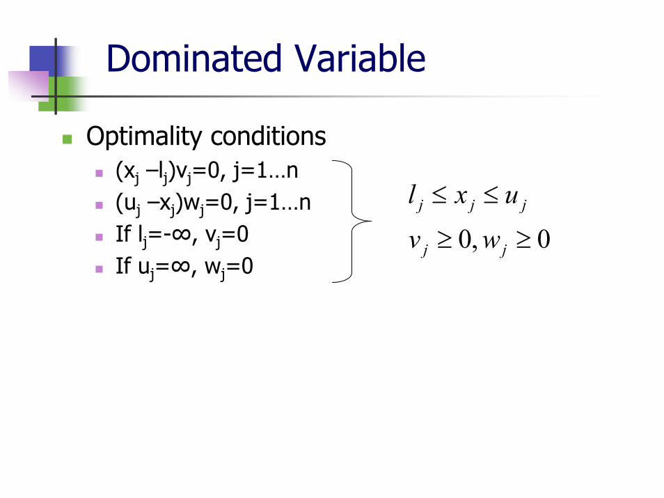
Optimality conditions(xj –lj)vj=0, j=1…n(uj –xj)wj=0, j=1…nIf lj=-∞, vj=0If uj=∞, wj=0
0,0 ≥≥
≤≤
jj
jjj
wv
uxl
Dominated Variable
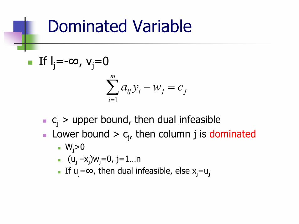
If lj=-∞, vj=0
cj > upper bound, then dual infeasible Lower bound > cj, then column j is dominated
Wj>0(uj –xj)wj=0, j=1…nIf uj=∞, then dual infeasible, else xj=uj
∑=
=−m
ijjiij cwya
1
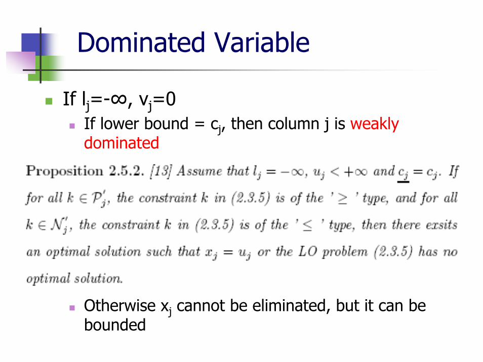
Dominated Variable
If lj=-∞, vj=0If lower bound = cj, then column j is weakly dominated
Otherwise xj cannot be eliminated, but it can be bounded
Dominated Variable
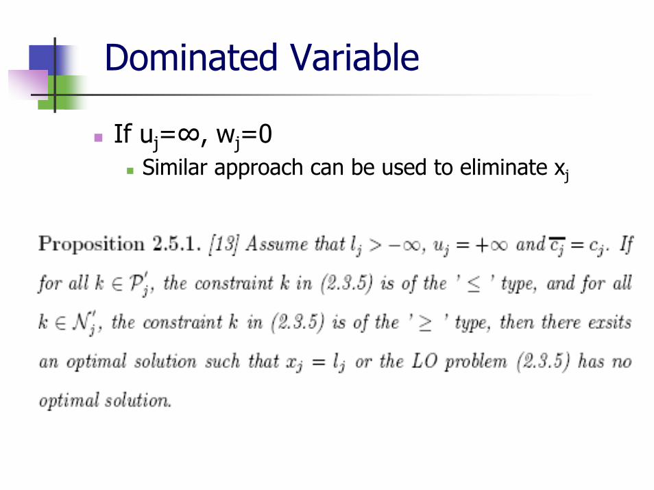
If uj=∞, wj=0Similar approach can be used to eliminate xj
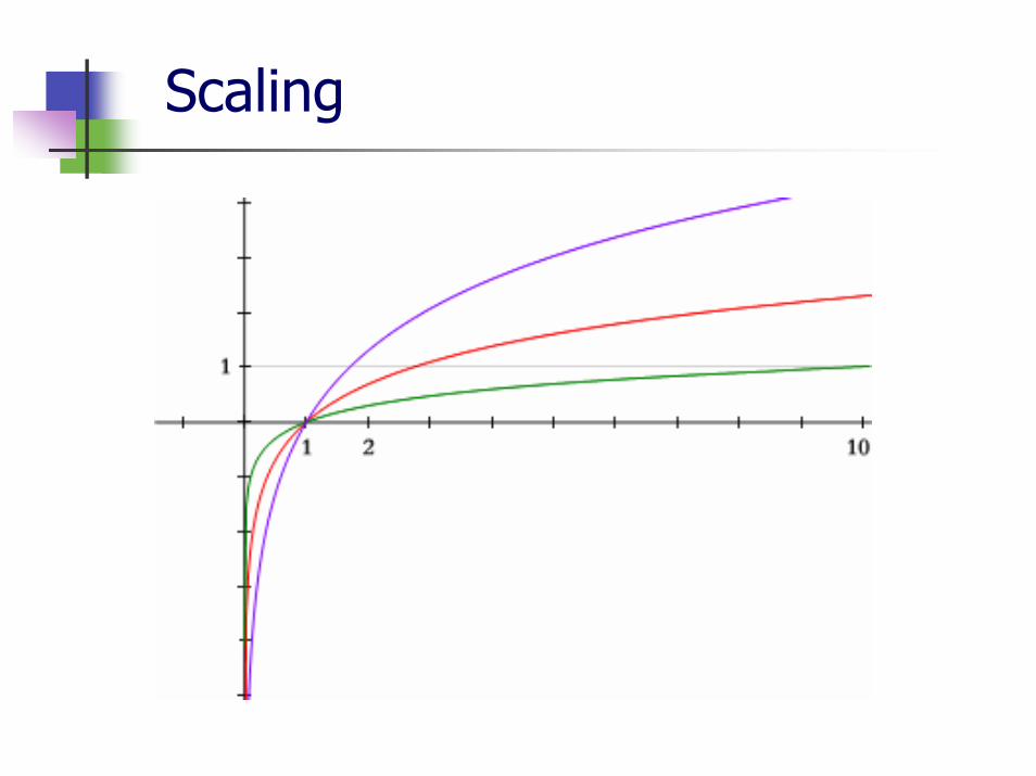
Scaling
Numerical difficulties arise if small and big numbers are present in A,b and cScaling adjusts the numerical characteristics to avoid such difficultiesAll data vectors must be scaledThe solution is unaffected
2x=8, 4x=16, 8x=32 all have the same solutionRows or columns can be scaled
RATx’=Rb, x=Tx’R=diag(r1,…,rm) ; T=diag(t1,…,tn)
Scaling
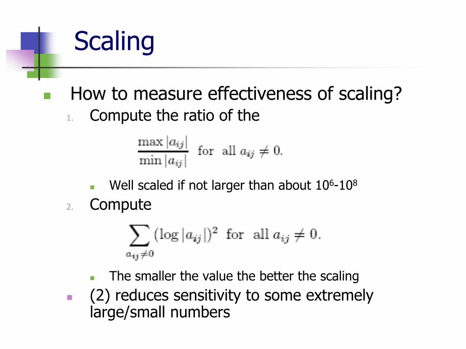
How to measure effectiveness of scaling?1. Compute the ratio of the
Well scaled if not larger than about 106-108
2. Compute
The smaller the value the better the scaling(2) reduces sensitivity to some extremely large/small numbers
Scaling
Scaling
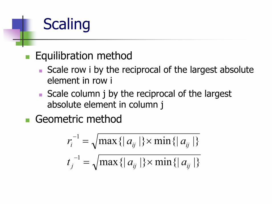
Equilibration methodScale row i by the reciprocal of the largest absolute element in row iScale column j by the reciprocal of the largest absolute element in column j
Geometric method
|}min{||}max{|
|}min{||}max{|1
1
ijijj
ijiji
aat
aar
×=
×=−
−
Scaling
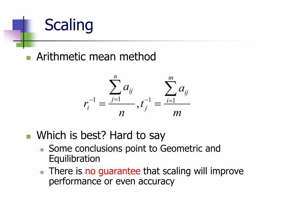
Arithmetic mean method
Which is best? Hard to saySome conclusions point to Geometric and EquilibrationThere is no guarantee that scaling will improve performance or even accuracy
m
at
n
ar
m
iij
j
n
jij
i
∑∑=−=− == 1111 ,
Advanced Preprocessing Techniques (Cont’d)
Alberto Olvera
Preprocessing Techniques
Advanced TechniquesDominated variablesTightening boundsScalingMake A Sparser (Reducing Sparsity)Finding Linear dependency (Full Rank)
Reducing Sparsity
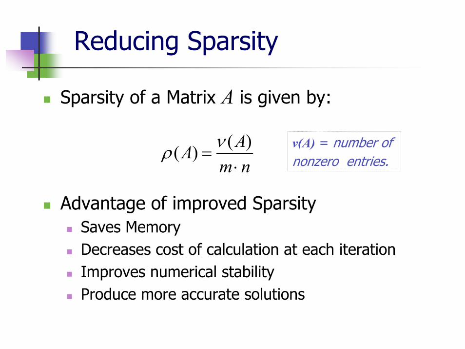
Sparsity of a Matrix A is given by:
Advantage of improved SparsitySaves MemoryDecreases cost of calculation at each iterationImproves numerical stabilityProduce more accurate solutions
nmAA⋅
=)()( νρ v(A) = number of
nonzero entries.
Reducing Sparsity (cont’d)
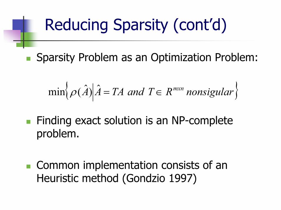
Sparsity Problem as an Optimization Problem:
Finding exact solution is an NP-complete problem.
Common implementation consists of an Heuristic method (Gondzio 1997)
{ }nonsigularRTandTAAA mxn∈=ˆ)ˆ(min ρ
Reducing Sparsity (cont’d)
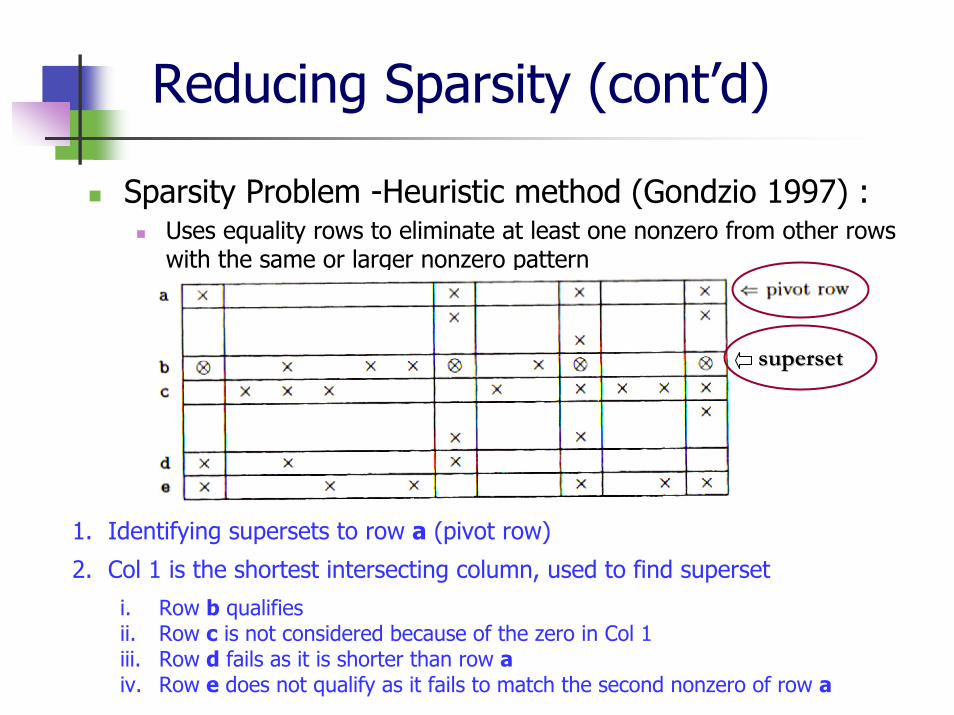
Sparsity Problem -Heuristic method (Gondzio 1997) :Uses equality rows to eliminate at least one nonzero from other rows with the same or larger nonzero pattern
1. Identifying supersets to row a (pivot row)
i. Row b qualifiesii. Row c is not considered because of the zero in Col 1iii. Row d fails as it is shorter than row aiv. Row e does not qualify as it fails to match the second nonzero of row a
2. Col 1 is the shortest intersecting column, used to find superset
supersetsuperset
Reducing Sparsity (cont’d)
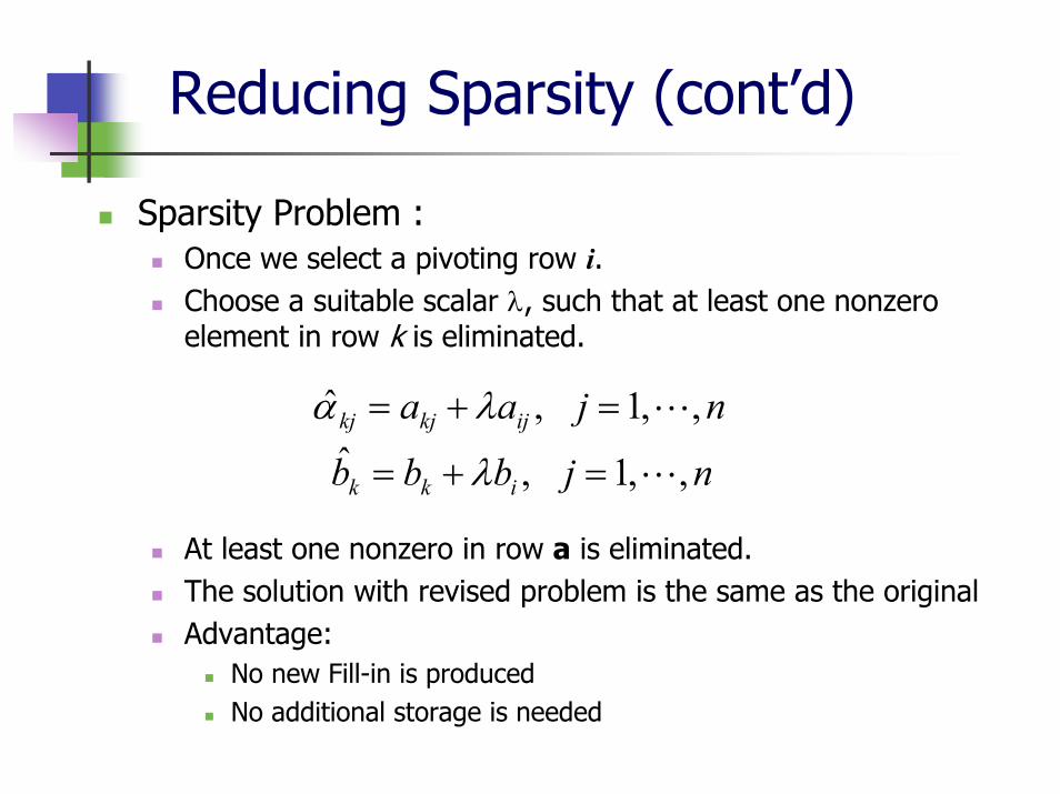
Sparsity Problem :Once we select a pivoting row i.Choose a suitable scalar λ, such that at least one nonzero element in row k is eliminated.
At least one nonzero in row a is eliminated.The solution with revised problem is the same as the originalAdvantage:
No new Fill-in is producedNo additional storage is needed
njaa ijkjkj ,,1,ˆ =+= λα
njbbb ikk ,,1,ˆ =+= λ
Making A Full Rank
Finding Linear dependency
Trivial reduction by identifying linearly dependent equalities.
Implemented efficiently based on Gaussian elimination
Advanced Techniques
Theoretically, Gaussian Elimination can be used to check the dependency of the rows.
For system A x = b, we combine matrix A(mxn) with vector b to get the matrix A = [A | b ] with the size of m(n+1).
A sequence of elementary row operations can be applied to the rows in matrix A to identify its rank.
Implementation goal:Avoid creating much fill-inKeep numerical stabilityObjective: just find linearly dependent rows

Preprocessing Scheme
The usual order of actions during preprocessing is:i. Problem Reformulationii. Presolveiii. Scaling
PresolveIt is not necessary to include all discussed techniquesSome more test from other references can be added.
Preprocessing Scheme
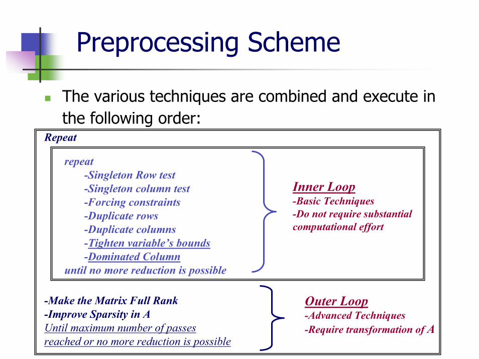
The various techniques are combined and execute in the following order:
Repeat
-Make the Matrix Full Rank-Improve Sparsity in AUntil maximum number of passes reached or no more reduction is possible
Outer Loop-Advanced Techniques-Require transformation of A
Inner Loop-Basic Techniques-Do not require substantial computational effort
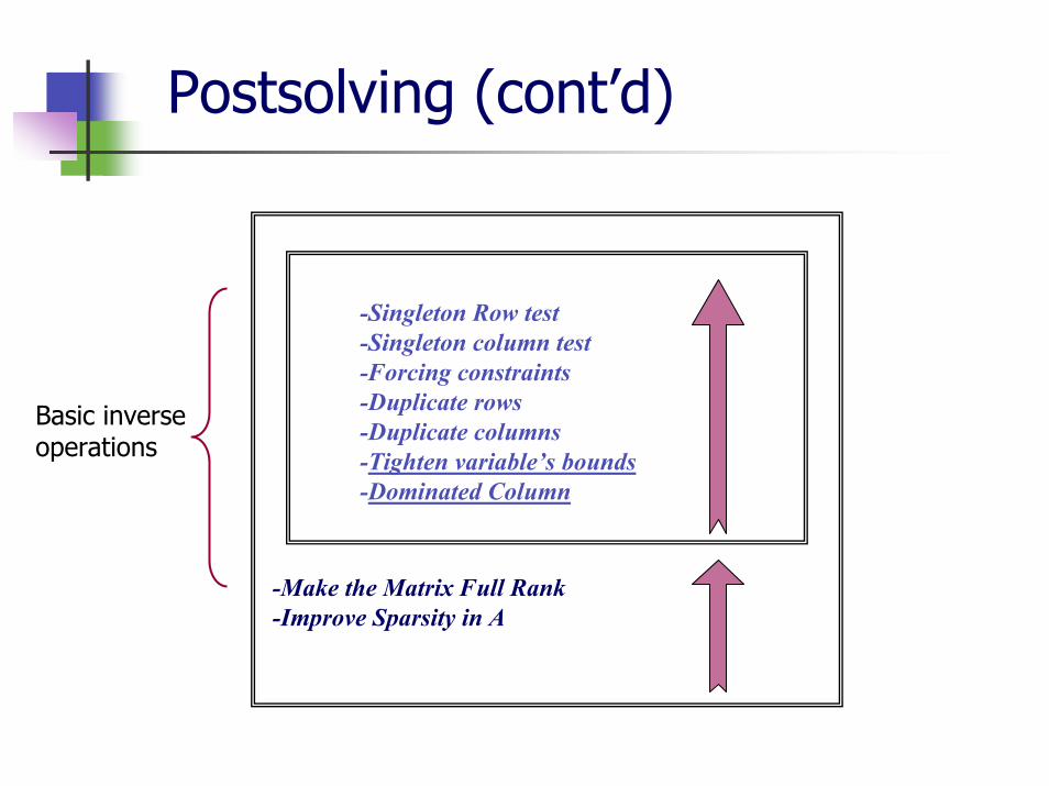
repeat-Singleton Row test -Singleton column test-Forcing constraints-Duplicate rows-Duplicate columns-Tighten variable’s bounds-Dominated Column
until no more reduction is possible
Preprocessing Scheme
Preprocessing Scheme
Significant part of the total reduction is done in the inner loop
In the outer loop the techniques require algebraic transformation of matrix A, therefore this are the most costly operations.
Postsolving
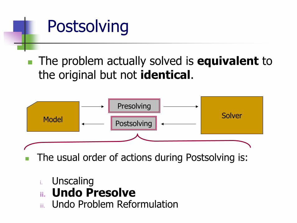
The problem actually solved is equivalent to the original but not identical.
Model SolverPostsolving
Presolving
The usual order of actions during Postsolving is:
i. Unscalingii. Undo Presolveiii. Undo Problem Reformulation
Postsolving
Postsolving operations are necessary after solving the preprocess problem.
Present a full primal-dual optimal solutions of the original solution.
from the optimal basis solution of the preprocessed problem.
Create an optimal basis solution of the original problem.
from the optimal basis solution of the preprocessed problem.
Postsolving (cont’d)
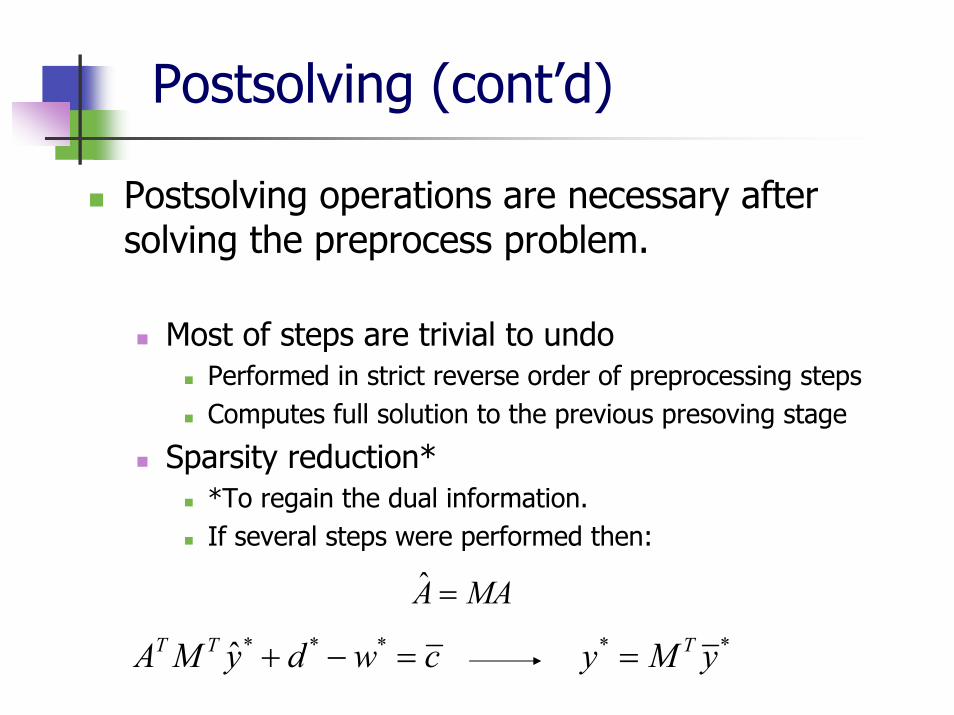
Postsolving operations are necessary after solving the preprocess problem.
Most of steps are trivial to undoPerformed in strict reverse order of preprocessing stepsComputes full solution to the previous presoving stage
Sparsity reduction**To regain the dual information.If several steps were performed then:
MAA =ˆ
cwdyMA TT =−+ ***ˆ ** yMy T=
Postsolving (cont’d)
-Make the Matrix Full Rank-Improve Sparsity in A
-Singleton Row test -Singleton column test-Forcing constraints-Duplicate rows-Duplicate columns-Tighten variable’s bounds-Dominated Column
Basic inverseoperations
Preprocessing in SDP
Jonathan Li
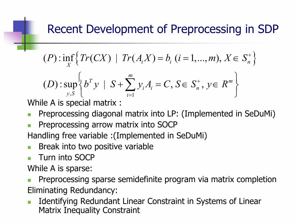
Recent Development of Preprocessing in SDP
While A is special matrix : Preprocessing diagonal matrix into LP: (Implemented in SeDuMi)Preprocessing arrow matrix into SOCP
Handling free variable :(Implemented in SeDuMi)Break into two positive variableTurn into SOCP
While A is sparse:Preprocessing sparse semidefinite program via matrix completion
Eliminating Redundancy:Identifying Redundant Linear Constraint in Systems of Linear Matrix Inequality Constraint
{ }
, 1
( ) : inf ( ) | ( ) ( 1,..., ),
( ) : sup | , ,
i i nX
mT m
i i ny S i
P Tr CX Tr A X b i m X S
D b y S y A C S S y R
+
+
=
= = ∈
⎧ ⎫+ = ∈ ∈⎨ ⎬
⎩ ⎭∑
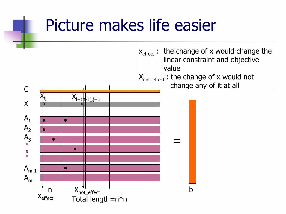
Picture makes life easier
A1
A2
A3
xeffect : the change of x would change the linear constraint and objective value
Xnot_effect : the change of x would not change any of it at all
Am-1
Am
X
Total length=n*nn
=
b
xij Xi+(n-1),j+1
xeffect
Xnot_effect
C
From LP to SDP
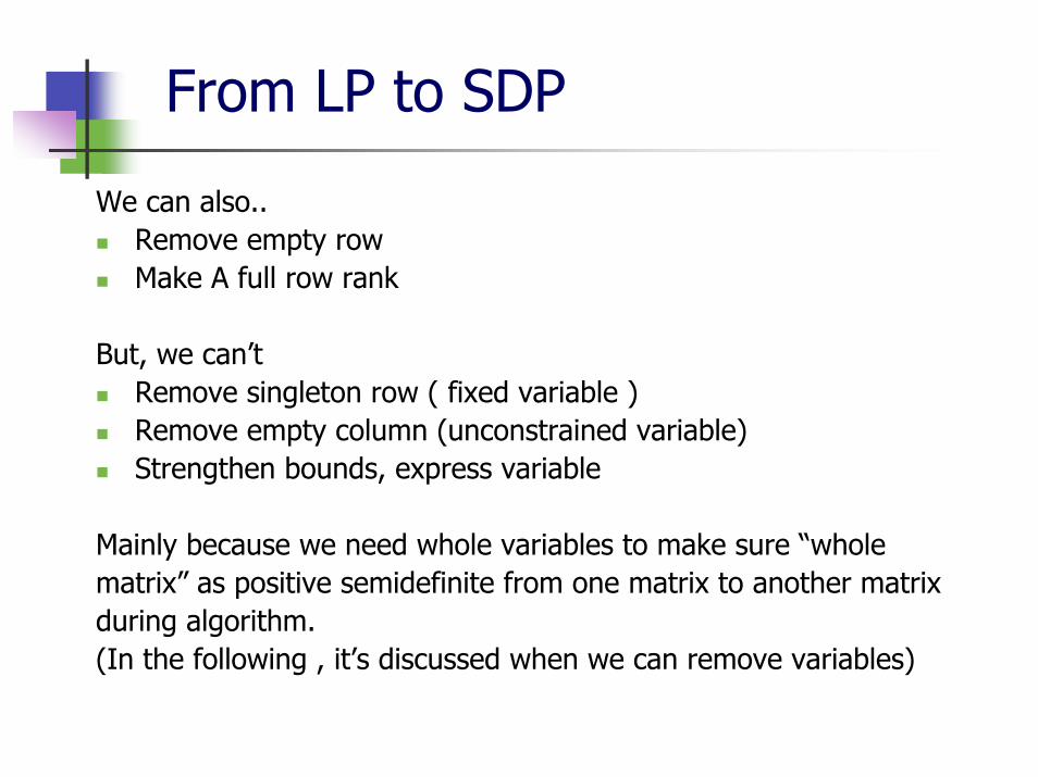
We can also..Remove empty row Make A full row rank
But, we can’t Remove singleton row ( fixed variable )Remove empty column (unconstrained variable)Strengthen bounds, express variable
Mainly because we need whole variables to make sure “whole matrix” as positive semidefinite from one matrix to another matrix during algorithm. (In the following , it’s discussed when we can remove variables)
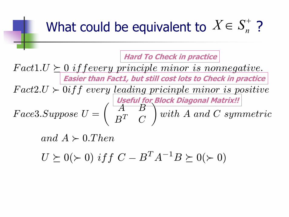
What could be equivalent to ?nX S +∈
Fact1.U º 0 iffevery principle minor is nonnegative.
Fact2.U Â 0iff every leading pricinple minor is positive
Face3.Suppose U =
µA BBT C
¶with A and C symmetric
and A Â 0.Then
U º 0(Â 0) iff C − BTA−1B º 0(Â 0)
Hard To Check in practice
Easier than Fact1, but still cost lots to Check in practice
Useful for Block Diagonal Matrix!!
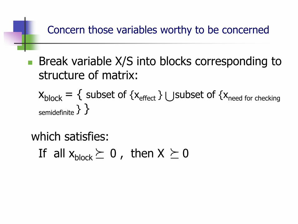
Concern those variables worthy to be concerned
Break variable X/S into blocks corresponding to structure of matrix:
xblock = { subset of {xeffect } subset of {xneed for checking
semidefinite } }
which satisfies:If all xblock 0 , then X 0
∪
º º
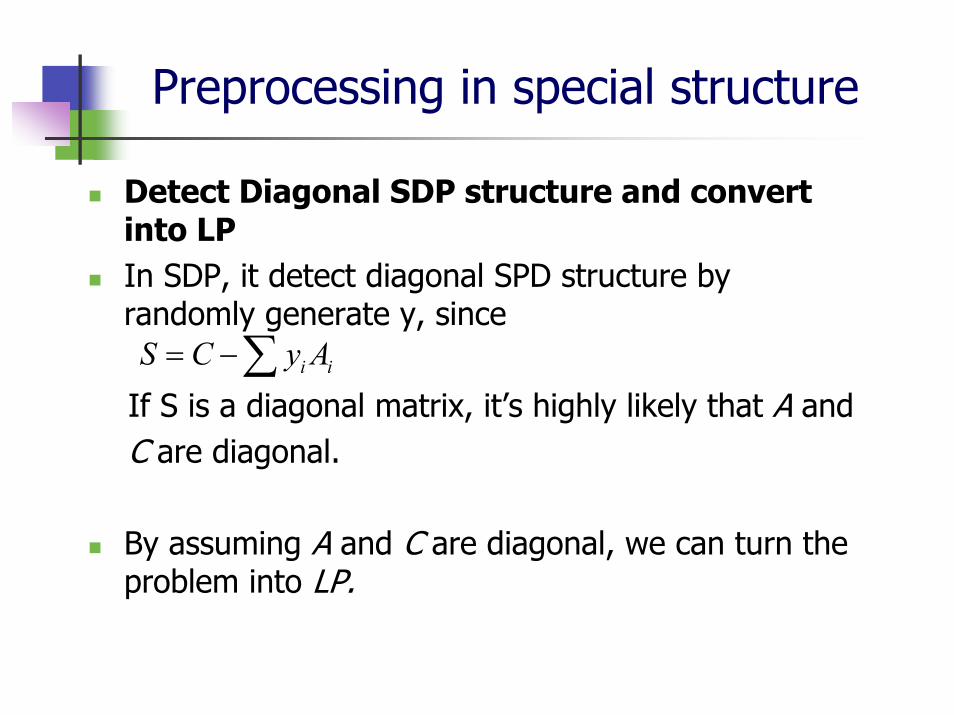
Preprocessing in special structure
Detect Diagonal SDP structure and convert into LP In SDP, it detect diagonal SPD structure by randomly generate y, since
If S is a diagonal matrix, it’s highly likely that A and C are diagonal.
By assuming A and C are diagonal, we can turn the problem into LP.
i iS C y A= −∑
Preprocessing in SeDuMi
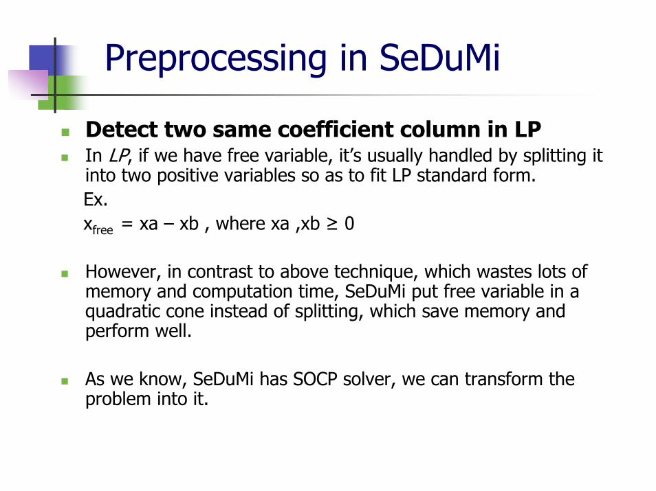
Detect two same coefficient column in LPIn LP, if we have free variable, it’s usually handled by splitting it into two positive variables so as to fit LP standard form.Ex.xfree = xa – xb , where xa ,xb ≥ 0
However, in contrast to above technique, which wastes lots of memory and computation time, SeDuMi put free variable in a quadratic cone instead of splitting, which save memory and perform well.
As we know, SeDuMi has SOCP solver, we can transform the problem into it.
Preprocessing sparse semidefinite program via matrix completion
In the paper : Preprocessing sparse semidefinite program via matrix completion, a heuristic is proposed to handle SDP problem while data matrix A is sparse.
Basic idea : Reduce the overload from computing and storing those “0” in sparse matrix.
Matrix completion : During computing, it tries to concern only those variablesaffecting linear part, in the mean time, it guarantees the feasibility of those variables being left out to eventually satisfy whole matrix as positive semidefinite.
Preprocessing sparse semidefinite program via matrix completion
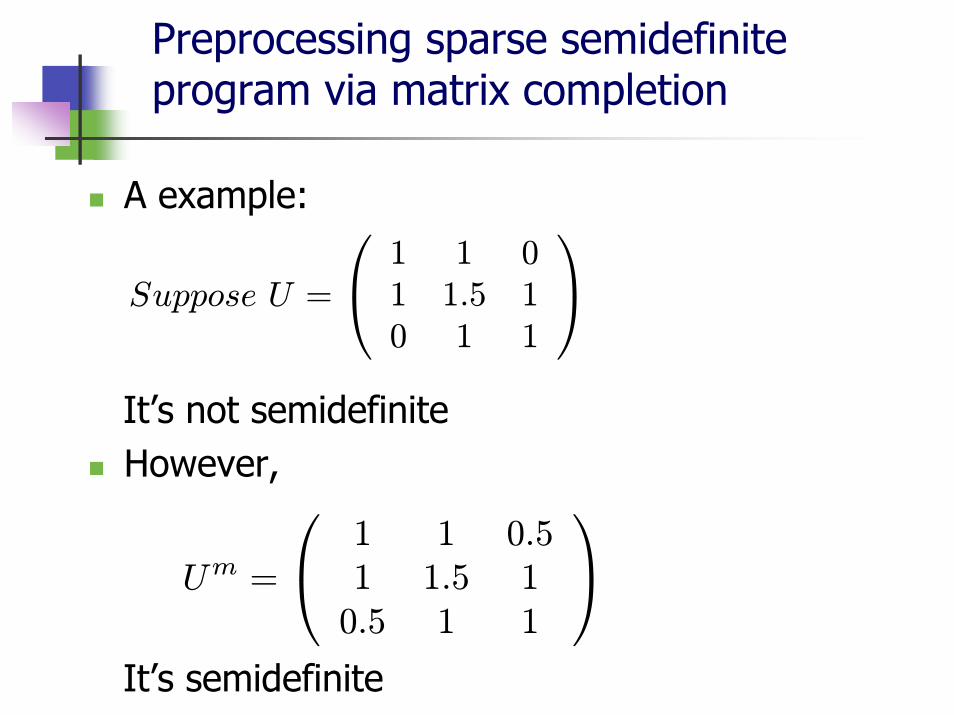
A example:
It’s not semidefiniteHowever,
It’s semidefinite
Suppose U =
⎛⎝ 1 1 01 1.5 10 1 1
⎞⎠
Um =
⎛⎝ 1 1 0.51 1.5 10.5 1 1
⎞⎠
Preprocessing sparse semidefinite program via matrix completion
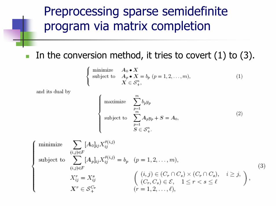
In the conversion method, it tries to covert (1) to (3).
Preprocessing sparse semidefinite program via matrix completion
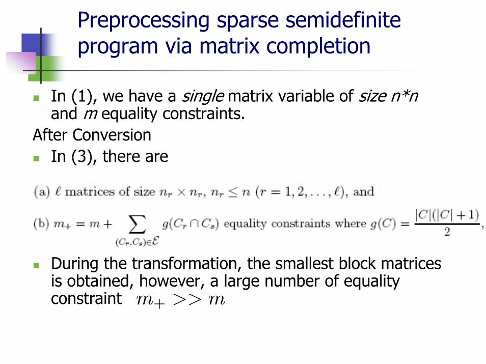
In (1), we have a single matrix variable of size n*nand m equality constraints.
After ConversionIn (3), there are
During the transformation, the smallest block matrices is obtained, however, a large number of equality constraint m+ >> m
Preprocessing sparse semidefinite program via matrix completion
One of the keys to obtaining a good conversion is to balance the factors (a) and (b) above to minimize the number of flops required by an SDP solver.
Eliminating Redundancy in SDP
Identifying Redundant Linear Constraint in Systems of Linear Matrix Inequality Constraint
In LP, eliminating redundant constraint is a basic technique, in SDP, it’s more difficult to eliminate Linear constraint when we take the cone into consideration also.
Eliminating Redundancy in SDP
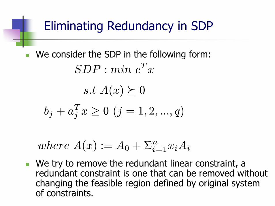
We consider the SDP in the following form:
We try to remove the redundant linear constraint, a redundant constraint is one that can be removed without changing the feasible region defined by original system of constraints.
SDP : min cTx
s.t A(x) º 0
bj + aTj x ≥ 0 (j = 1, 2, ..., q)
where A(x) := A0 + Σni=1xiAi
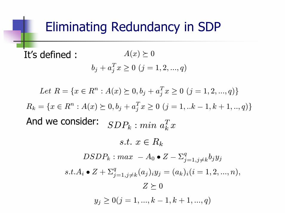
Eliminating Redundancy in SDP
A(x) º 0
bj + aTj x ≥ 0 (j = 1, 2, ..., q)
Let R = {x ∈ Rn : A(x) º 0, bj + aTj x ≥ 0 (j = 1, 2, ..., q)}
Rk = {x ∈ Rn : A(x) º 0, bj + a
Tj x ≥ 0 (j = 1, ..k − 1, k + 1, .., q)}
It’s defined :
And we consider: SDPk : min aTk x
s.t. x ∈ Rk
DSDPk : max − A0 • Z − Σqj=1,j 6=kbjyj
s.t.Ai • Z + Σqj=1,j 6=k(aj)iyj = (ak)i(i = 1, 2, ..., n),
Z º 0
yj ≥ 0(j = 1, ..., k − 1, k + 1, ..., q)
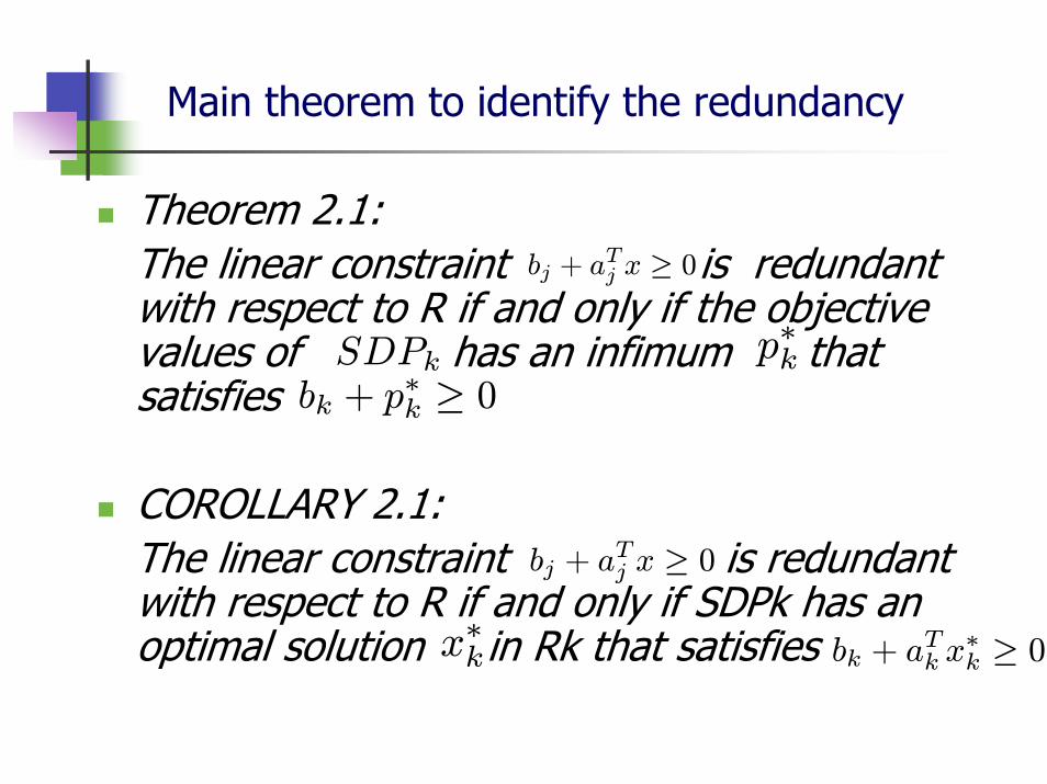
Main theorem to identify the redundancy
Theorem 2.1:The linear constraint is redundant with respect to R if and only if the objective values of has an infimum that satisfies
COROLLARY 2.1:The linear constraint is redundant with respect to R if and only if SDPk has an optimal solution in Rk that satisfies
bj + aTj x ≥ 0
SDPk p∗kbk + p
∗k ≥ 0
bj + aTj x ≥ 0
x∗k bk + aTk x∗k ≥ 0
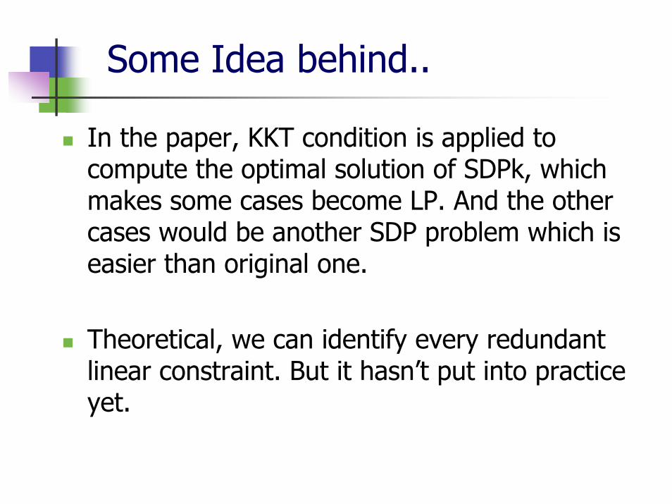
Some Idea behind..
In the paper, KKT condition is applied to compute the optimal solution of SDPk, which makes some cases become LP. And the other cases would be another SDP problem which is easier than original one.
Theoretical, we can identify every redundant linear constraint. But it hasn’t put into practice yet.
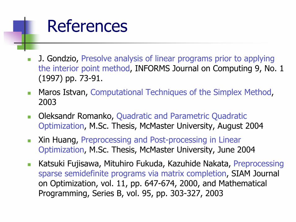
References
J. Gondzio, Presolve analysis of linear programs prior to applying the interior point method, INFORMS Journal on Computing 9, No. 1 (1997) pp. 73-91.
Maros Istvan, Computational Techniques of the Simplex Method, 2003
Oleksandr Romanko, Quadratic and Parametric Quadratic Optimization, M.Sc. Thesis, McMaster University, August 2004
Xin Huang, Preprocessing and Post-processing in Linear Optimization, M.Sc. Thesis, McMaster University, June 2004
Katsuki Fujisawa, Mituhiro Fukuda, Kazuhide Nakata, Preprocessing sparse semidefinite programs via matrix completion, SIAM Journal on Optimization, vol. 11, pp. 647-674, 2000, and Mathematical Programming, Series B, vol. 95, pp. 303-327, 2003