28 Noiembrie 2019 1

Prelucrarea Imaginilor

Curs 9

2/36

Sistemul RGB Este posibil să reprezentăm o

culoare prin trei coordonate

(numere naturale) reprezentând

cantităţile culorilor de bază, de

exemplu roşu, verde şi albastru

(Red, Green, Blue), deci în

spaţiul RGB (vezi figura 2.2.5)

sau cel complementar (Cyan,

Yellow, Magenta). Utilizând opt

bit pentru reprezentarea fiecărei

coordonate (valori a compo-

nentei red, green sau blue)

vom obţine un spaţiu al culorilor

cu valori din domeniul [0..255]3,

adică 224 valori distincte, deci

peste 16 milioane de nuanţe .

R

G

B

Alb

Negru

Cyan

Yellow

Magenta

C(r,g,b)

b

g

r

Spaţiul culorilor în sistemul RGB

3/36

Sistemul RGB

Spectrul este o bandă contiuă de lungimi de undă emisă,

reflectată sau transmisă de deverse obiecte. Ochiul uman nu poate

vedea întregul spectru, doar culori cu valori din domeniul [400nm-

700nm] corespunzător [albastru-roşu]. În practică, spectrul este

reprezentat ca un vector de numere care măsoară intensitatea

diferitelor lungimi de undă. Usual, un spectrofotometru are o

rezoluţie de 1-3 nm, măsurând de la 100 la 300 de valori pentru a

măsura domeniul vizibil. Presupunând că un aparat foarte simplu

scanează un spectru la fiecare 3 nm (100 de puncte pentru 300 nm)

şi măsoară fiecare punct cu o precizie de doar 8 bit. Aceasta

înseamnă că aparatul poate distinge mai mult de 10240 de spectre

diferite (atâtea numere pot fi codificate pe 8 bit x 100 puncte = 800

bit de date). Dar oamenii pot distinge doar în jur de 10 milioane de

culori. Aceasta se întâmplă pentru că ochiul are doar trei tipuri de

conuri receptoare în retină care răspund diferitelor lungimi de undă a

luminii. Astfel, creierul receptează doar trei semnale pentru fiecare

spectru, acestea dându-ne percepţia culorii.

4/36

Interpretări colorimetrice computerizate

Un sistem tricromatic poate defini orice culoare combinaţia a trei

culori de bază în cantitati unic precizate (culorile fundamentale sunt

alese astfel încât nici una să nu poatăfi obţinută prin amestecul

celorlaltor două). Cel mai cunoscut sistem tricromatic este sistemul RVI

(R-rosu, V-verde, I-indigo) caracterizat prin cele trei culori de bază

având următoarele lungimi de undă: rosu =700 nm; verde =546,1

nm; indigo = 435 nm.

Orice culoare monocromatică spectrală, într-un sistem tricromatic este

caracterizată prin trei valori numite valori spectrale sau coeficienţi de

distribuţie. În sistemul RVI, există culori care sunt caracterizate şi prin

coeficienţi negativi (coordonate negative ale culorilor de bază). Pentru a

elimina valorile negative la precizarea unei culori, s-au definit trei culori

virtuale (notate cu X, Y, Z) care nu mai prezintă inconvenientul precizat.

Aceste culori constitue valorile fundamentale ale culorii în sistemul

tricromatic CIE (Commission Internationale De L’Eclairage), fiind

denumite şi coordonate tricromatice sau valori tristimu.

5/36

Caracterizarea şi măsurarea culorilor

în sisteme tricromatice

În sistemul CIE, o culoare poate fi reprezentată grafic într-un sistem

tridimensional prin punctul de coordonate (X,Y,Z). Totalitatea punctelor ce

corespund tuturor culorilor posibile constituie spaţiul culorilor.

X

Z

Y

540

510

580

500

700

780

490

380

Spaţiul culorilor în sistemul de coordonate X,Y,Z (CIE).

6/36

Caracterizarea şi măsurarea culorilor în sisteme tricromatice

Măsurarea culorilor în sistemul CIE constă în determinarea valorilor

X,Y,Z. În acest scop se consideră cei trei factori care caracterizează

culoarea, şi anume:

• iluminantul, reprezentat prin curba de distribuţie a energiei E();

• corpul colorat, reprezentat prin curbele de remisiune (reflexie) R();

• ochiul omenesc caracterizat prin curbele de distribuţie spectrală pentru

observatorul normal x(), y(), z().

Pentru o lungime de undă , energia transmisă de corpul colorat

este egală cu produsul E()R().

Energia transmisă pentru toate lungimile de undă ale spectrului

vizibil () este egală cu E()R(), şi reprezintă interacţiunea iluminant-corp.

7/36

Caracterizarea şi măsurarea culorilor în sisteme

tricromatice

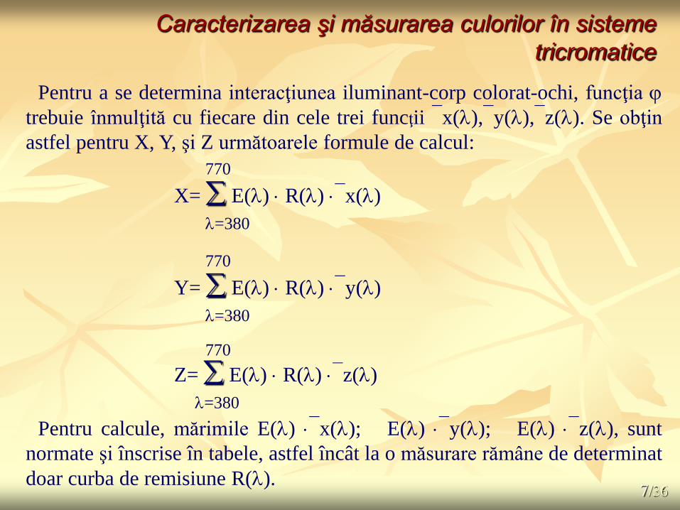
Pentru a se determina interacţiunea iluminant-corp colorat-ochi, funcţia

trebuie înmulţită cu fiecare din cele trei funcţii x(),y(),z(). Se obţin

astfel pentru X, Y, şi Z următoarele formule de calcul:

770

X= E() R() x()

=380

770

Y= E() R() y()

=380

770

Z= E() R() z()

=380

Pentru calcule, mărimile E() x(); E() y(); E() z(), sunt

normate şi înscrise în tabele, astfel încât la o măsurare rămâne de determinat

doar curba de remisiune R().

8/36

Caracterizarea şi măsurarea culorilor în sisteme tricromatice

Pentru sistemul CIELAB 76,

coordonatele tricromatice X, Y, Z sunt

transformate în alte trei coordonate:

L* (coordonata luminozitate),

a* (coordonata roşu-verde) şi

b* (coordonata galben-albastru) :

unde X0, Y0 şi Z0 sunt coordonatele

tricromatice care se obţin în cazul unui

material cu suprafaţă reflectantă perfect

albă:

L*=116 · f (Y/Y0);

a* =500 · [ f(X/X0) - f (Y/Y0)]

b* =200 · [f (Y/Y0) - f (Z /Z0)]

770

X0= E() x()

=380

770

Y0= E() y()

=380

770

Z0= E() z() =380

iar f()=1/3- 16/116 .

9/36

Caracterizarea şi măsurarea culorilor în sisteme tricromatice

Diferenţa de culoare E* dintre două culori (probe) reprezintă

distanţa geometrică (Euclidiană) dintre punctele corespunzătoare

(celor două probe) din spaţiul culorilor. În sistemul CIELAB, aceasta

se calculează cu ajutorul formulei:

E* = (L*2 + a*2 + b*2 )1/2

unde:

L* reprezintă diferenţa de luminozitate dintre cele două probe,

a* reprezintă diferenţa dintre coordonatele roşu-verde,

b* reprezintă diferenţa dintre coordonatele .galben-albastru.

10/36

Vizualizarea culorilor (http://www.cambridgeincolour.com/tutorials.htm)

Pe verticala este masurata luminozitatea, iar pe orizontala rosu-

verde, respectiv galben-albastru:

Spatiul CIE al

culorilor vizibile:

CIE XYZ (1931) CIE L a*b* CIE L u'v' (1976)

11/36

RGB L a*b* & L a*b* RGB

R 3.240479 -1.537150 -0.498535 X

G = -0.969256 1.875992 0.041556 * Y

B 0.055648 -0.204043 1.057311 Z .

XYZ RGB

RGB XYZ

X 0.412453 0.357580 0.180423 R

Y = 0.212671 0.715160 0.072169 * G

Z 0.019334 0.119193 0.950227 B .

L* = 116 * (Y/Yn)1/3 - 16 pentru Y/Yn > 0.008856

L* = 903.3 * Y/Yn altfel

a* = 500 * ( f(X/Xn) - f(Y/Yn) )

b* = 200 * ( f(Y/Yn) - f(Z/Zn) )

unde f(t) = t1/3 pentru t > 0.008856

f(t) = 7.787 * t + 16/116 altfel

XYZ L a*b*

X = Xn * ( P + a* / 500 )3

Y = Yn * P3

Z = Zn * ( P - b* / 200 )3

unde P = (L* + 16) / 116

L a*b* XYZ

12/36

RGB XYZ L a*b* void Tr(float& C) { C/=255.; if (C>0.04045) C=x_la_y((C+0.055)/1.055,2.4); else C/=12.92; C=C*100; } void RGB_XYZ(float R,float G,float B, float& X, float& Y,float& Z) { Tr(R); Tr(G); Tr(B); X=R * 0.4124 + G * 0.3576 + B * 0.1805; Y=R * 0.2126 + G * 0.7152 + B * 0.0722; Z=R * 0.0193 + G * 0.1192 + B * 0.9505; } float f(float t) { float e=0.008856; if (t>e) return x_la_y(t,1/3.); else return 7.787*t+16./116.; } void XYZ_Lab(float X, float Y, float Z, float& L, float& a, float& b) { float Xn, Yn, Zn; float W=255.; float e=0.008856; RGB_XYZ(W,W,W,Xn,Yn,Zn); X=X/Xn; Y=Y/Yn; Z=Z/Zn; if (Y>e) L=116.*x_la_y(Y,1/3.)-16; else L=903.3*Y; a=500.*(f(X)-f(Y)); b=200.*(f(Y)-f(Z)); }

RGB_XYZ(R,G,B, vX,vY,vZ);

XYZ_Lab(vX,vY,vZ, LL,aa,bb);

13/36

L a*b* XYZ RGB http://www.easyrgb.com/index.php?X=MATH

void Tr1(float& C)

{ if ( C3 > 0.008856 ) C = C3 else C = ( C - 16 / 116 ) / 7.787 }

var_Y = ( CIE-L* + 16 ) / 116 // Observer= 2°, Illuminant= D65

var_X = CIE-a* / 500 + var_Y

var_Z = var_Y - CIE-b* / 200

Tr1(Var_X); Tr1(Var_Y); Tr1(Var_Z);

X = ref_X * var_X //ref_X = 95.047

Y = ref_Y * var_Y //ref_Y = 100.000

Z = ref_Z * var_Z //ref_Z = 108.883

L a*b* XYZ

XYZ RGB

void Tr2(float& C)

{ if ( C > 0.0031308 ) C = 1.055 * C1 / 2.4 - 0.055 else C = 12.92 * C }

var_X = X / 100 //X from 0 to 95.047 (Observer = 2°, Illuminant = D65)

var_Y = Y / 100 //Y from 0 to 100.000

var_Z = Z / 100 //Z from 0 to 108.883

var_R = var_X * 3.2406 + var_Y * -1.5372 + var_Z * -0.4986

var_G = var_X * -0.9689 + var_Y * 1.8758 + var_Z * 0.0415

var_B = var_X * 0.0557 + var_Y * -0.2040 + var_Z * 1.0570

Tr2(var_R); Tr2(var_G); Tr2(var_B);

R = var_R * 255; G = var_G * 255; B = var_B * 255

14/36

RGB Luv & Luv RGB

unde:

u = 4*X / (X + 15*Y + 3*Z)

v = 9*Y / (X + 15*Y + 3*Z)

un = 4*x

n / (-2*x

n + 12*y

n + 3)

vn = 9*y

n / (-2*x

n + 12*y

n + 3)

L = 116 * (Y/Yn)1/3 - 16

U = 13 * L * (u - un)

V = 13 * L * (v - vn)

RGB CIE-Luv

După conversia din spaţiul RGB în XYZ (descrisă anterior) se va

efectua conversia în spaţiul CIE Luv astfel:

15/36

apoi, se va efectua conversia în spaţiul RGB (descrisă anterior).

unde:

u = U / (13*L) + un

v = V / (13*L) + vn

Y = Yn * ((L+16)/116)3

X = -9*Y*u/((u-4)*v - u*v)

Z = (9*Y - 15*v*Y - v*X)/3*v

CIE-Luv RGB

Mai întăi vom efectua conversia din spaţiul CIE Luv în spaţiul XYZ:

RGB Luv & Luv RGB

16/36

Color space

A color model is an abstract mathematical model describing the

way colors can be represented as tuples of numbers, typically as three or four

values orcolor components (e.g. RGB and CMYK are color models). However,

a color model with no associated mapping function to an absolute color space is

a more or less arbitrary color system with no connection to any globally-

understood system of color interpretation.

Adding a certain mapping function between the color model and a certain

reference color space results in a definite "footprint" within the reference color

space. This "footprint" is known as a gamut, and, in combination with the color

model, defines a new color space. For example, Adobe RGB and sRGBare two

different absolute color spaces, both based on the RGB model.

In the most generic sense of the definition above, color spaces can be defined

without the use of a color model. These spaces, such as Pantone, are in effect a

given set of names or numbers which are defined by the existence of a

corresponding set of physical color swatches. This article focuses on the

mathematical model concept.

17/36

Understanding the concept A wide range of colors can be created by the primary colors of pigment

(cyan (C), magenta (M), yellow (Y), and black (K)). Those colors then define a

specific color space. To create a three-dimensional representation of a color

space, we can assign the amount of magenta color to the representation's Xaxis,

the amount of cyan to its Y axis, and the amount of yellow to its Z axis. The

resulting 3-D space provides a unique position for every possible color that can

be created by combining those three pigments.

However, this is not the only possible color space. For instance, when colors

are displayed on a computer monitor, they are usually defined in the RGB

(red, green and blue) color space. This is another way of making nearly the same

colors (limited by the reproduction medium, such as the phosphor (CRT) or

filters and backlight (LCD)), and red, green and blue can be considered as the X,

Y and Z axes. Another way of making the same colors is to use theirHue (X

axis), their Saturation (Y axis), and their brightness Value (Z axis). This is called

the HSV color space. Many color spaces can be represented as three-

dimensional (X,Y,Z) values in this manner, but some have more, or fewer

dimensions, and some cannot be represented in this way at all..

18/36

Conversion When formally defining a color space, the usual reference standard is

the CIELAB or CIEXYZ color spaces, which were specifically designed to

encompass all colors the average human can see.

Since "color space" is a more specific term for a certain combination of a

color model plus a mapping function, the term "color space" tends to be used to

also identify color models, since identifying a color space automatically

identifies the associated color model. Informally, the two terms are often used

interchangeably, though this is strictly incorrect. For example, although several

specific color spaces are based on the RGB model, there is no such thing

as the RGB color space.

Since any color space defines colors as a function of the absolute reference

frame, color spaces, along with device profiling, allow reproducible

representations of color, in both analogue and digitalrepresentations.

Color space conversion is the translation of the representation of a color from

one basis to another. This typically occurs in the context of converting an image

that is represented in one color space to another color space, the goal being to

make the translated image look as similar as possible to the original.

19/36

Some color spaces CIE 1931 XYZ color space was one of the first attempts to produce a color

space based on measurements of human color perception (earlier efforts were by James Clerk Maxwell, König & Dieterici, and Abney at Imperial College)[1] and it is the basis for almost all other color spaces. Derivatives of the CIE XYZ space include CIELUV, CIEUVW, and CIELAB.

RGB uses additive color mixing,

because it describes what kind

of light needs to be emitted to produce a

given color. Light is added together to

create form from out of the darkness. RGB

stores individual values for red, green and

blue. RGBA is RGB with an additional

channel, alpha, to indicate transparency.

Common color spaces based on the RGB

model include sRGB, Adobe

RGB and ProPhoto RGB.

20/36

Some color spaces

CMYK uses subtractive color mixing

used in the printing process, because it

describes what kind of inks need to be

applied so the light reflected from the

substrate and through the inks produces a

given color. One starts with a white

substrate (canvas, page, etc), and uses ink

to subtract color from white to create an

image. CMYK stores ink values for cyan,

magenta, yellow and black. There are

many CMYK color spaces for different

sets of inks, substrates, and press

characteristics (which change the dot

gain or transfer function for each ink and

thus change the appearance).

21/36

Some color spaces

A comparison of RGB and CMYK color spaces.

The image demonstrates the difference between

the RGB and CMYK color gamuts. The CMYK

color gamut is much smaller than the RGB color

gamut, thus the CMYK colors look muted. If you

were to print the image on a CMYK device (an

offset press or maybe even a ink jet printer) the

two sides would likely look much more similar,

since the combination of cyan, yellow, magenta

and black cannot reproduce the range (gamut) of

color that a computer monitor displays. This is a

constant issue for those who work in print

production. Clients produce bright and colorful

images on their computers and are disappointed

to see them look muted in print. (An exception is

photo processing. In photo processing, like

snapshots or 8x10 glossies, most of the RGB

gamut is reproduced.)

A comparison of RGB and

CMYK color models. This

image demonstrates the

difference between how colors

will look on a computer

monitor (RGB) compared to

how they will reproduce in a

CMYK print process.

22/36

Generic color spaces YIQ was formerly used in NTSC (North America, Japan and elsewhere)

television broadcasts for historical reasons. This system stores a luminance value with two chrominance values, corresponding approximately to the amounts of blue and red in the color. It is similar to the YUV scheme used in most video capture systems[2] and in PAL (Australia, Europe, except France, which uses SECAM) television, except that the YIQ color space is rotated 33° with respect to the YUV color space. The YDbDr scheme used by SECAM television is rotated in another way.

YPbPr is a scaled version of YUV. It is most commonly seen in its digital form, YCbCr, used widely in video and image compression schemes such asMPEG and JPEG.

xvYCC is a new international digital video color space standard published by the IEC (IEC 61966-2-4). It is based on the ITU BT.601 and BT.709 standards but extends the gamut beyond the R/G/B primaries specified in those standards.

HSV (hue, saturation, value), also known as HSB (hue, saturation, brightness) is often used by artists because it is often more natural to think about a color in terms of hue and saturation than in terms of additive or subtractive color components. HSV is a transformation of an RGB colorspace, and its components and colorimetry are relative to the RGB colorspace from which it was derived.

HSL (hue, saturation, lightness/luminance), also known as HLS or HSI (hue, saturation, intensity) is quite similar to HSV, with "lightness" replacing "brightness". The difference is that the brightness of a pure color is equal to the brightness of white, while the lightness of a pure color is equal to the lightness of a medium gray.

23/36

HSL and HSV

HSL and HSV are the two most common cylindrical-coordinate representations

of points in an RGB color model, which rearrange the geometry of RGB in an

attempt to be more perceptually relevant than the cartesian representation. They

were developed in the 1970s for computer graphics applications, and are used

for color pickers, in color-modification tools inimage editing software, and less

commonly for image analysis and computer vision.

HSL stands for hue, saturation, and lightness, and is often also called HLS.

HSV stands for hue, saturation, and value, and is also often

called HSB (B for brightness). A third model, common in computer

vision applications, is HSI, for hue,saturation, and intensity. Unfortunately, while

typically consistent, these definitions are not standardized, and any of these

abbreviations might be used for any of these three or several other related

cylindrical models. (For technical definitions of these terms, see below.)

Both of these representations are used widely in computer graphics, and one or

the other of them is often more convenient than RGB, but both are also commonly

criticized for not adequately separating color-making attributes, or for their lack

ofperceptual uniformity. Other more computationally intensive models, such

as CIELAB or CIECAM02 better achieve these goals.

24/36

HSL and HSV

In each cylinder, the angle around the central vertical axis corresponds to “hue”, the distance from the axis corresponds to “saturation”, and the distance along the axis corresponds to “lightness”, “value” or “brightness”. Note that while “hue” in HSL and HSV refers to the same attribute, their definitions of “saturation” differ dramatically.

Because HSL and HSV are simple transformations of device-dependent RGB models, the physical colors they define depend on the colors of the red, green, and blue primaries of the device or of the particular RGB space, and on the gamma correction used to represent the amounts of those primaries. Each unique RGB device therefore has unique HSL and HSV spaces to accompany it, and numerical HSL or HSV values describe a different color for each basis RGB space.

HSL and HSV cylinder

25/36

HSL and HSV Basic idea

HSL and HSV are both cylindrical geometries, with hue,

their angular dimension, starting at the red primary at 0°,

passing through the green primary at 120° and

the blue primary at 240°, and then wrapping back to red at

360°. In each geometry, the central vertical axis comprises

the neutral, achromatic, or gray colors, ranging from

black at lightness 0 or value 0, the bottom, to white at

lightness 1 or value 1, the top. In both geometries,

the additive primary and secondary colors –

red, yellow, green, cyan, blue, and magenta – and linear

mixtures between adjacent pairs of them, sometimes

called pure colors, are arranged around the outside edge of the

cylinder with saturation 1; in HSV these have value 1 while in

HSL they have lightness ½. In HSV, mixing these pure colors

with white – producing so-called tints – reduces saturation,

while mixing them with black – producing shades – leaves

saturation unchanged. In HSL, both tints and shades have full

saturation, and only mixtures with both black and white –

called tones – have saturation less than 1.

HSV cylinder

HSL cylinder

26/36

HSL and HSV Basic idea

Because these definitions of saturation – in which very dark (in both models) or very

light (in HSL) near-neutral colors, for instance Black or White, are considered fully

saturated – conflict with the intuitive notion of color purity, often a conic or bi-conic solid

is drawn instead, with what this article calls chroma as its radial dimension, instead of

saturation. Confusingly, such diagrams usually label this radial dimension “saturation”,

blurring or erasing the distinction between saturation and chroma. As described below,

computing chroma is a helpful step in the derivation of each model. Because such an

intermediate model – with dimensions hue, chroma, and HSV value or HSL lightness –

takes the shape of a cone or bicone, HSV is often called the “hexcone model” while HSL is

often called the “bi-hexcone model”

If we plot hue and (a) HSL lightness or (b) HSV value against chroma rather than

saturation, the resulting solid is a bicone or cone, not a cylinder. Such diagrams often claim

to represent HSL or HSV directly, with the chroma dimension labeled “saturation”.

27/36

HSL and HSV

Lightness

While the definition of hue is relatively uncontroversial – it roughly satisfies the

criterion that colors of the same perceived hue should have the same numerical hue – the

definition of a lightness or value dimension is less obvious: there are several possibilities

depending on the purpose and goals of the representation. Here are four of the most

common :

• The simplest definition is just the average of the three components, in the HSI model

called intensity (fig. 11a). This is simply the projection of a point onto the neutral axis –

the vertical height of a point in our tilted cube. The advantage is that, together with

Euclidean-distance calculations of hue and chroma, this representation preserves distances

and angles from the geometry of the RGB cube.

I = (R + G + B ) / 3

In the HSV “hexcone” model, value is defined as the largest component of a color,

our M above (fig. 11b). This places all three primaries, and also all of the “secondary

colors” – cyan, yellow, and magenta – into a plane with white, forming a hexagonal

pyramid out of the RGB cube.

V = M

28/36

HSL and HSV

Lightness

• In the HSL “bi-hexcone” model, lightness is defined as the average of the largest and

smallest color components (fig. 11c). This definition also puts the primary and secondary

colors into a plane, but a plane passing halfway between white and black. The resulting

color solid is a double-cone similar to Ostwald’s, shown above.

L = (M + m) / 2

• A more perceptually relevant alternative is to use luma, Y′, as a lightness dimension

(fig. 11d). Luma is the weighted average of gamma-corrected R, G, and B, based on

their contribution to perceived luminance, long used as the monochromatic dimension

in color television broadcast.

• For the Rec. 709 primaries used in sRGB, Y′709 = .21R + .72G + .07B;

• for the Rec. 601 NTSC primaries, Y′601 = .30R + .59G + .11B;

• for other primaries different coefficients should be used.

Y’601=0.3*R + 0.59*G + 0.11*B

All four of these leave the neutral axis alone. That is, for colors with R = G = B, any

of the four formulations yields a lightness equal to the value of R, G, or B.

29/36

HSL and HSV

Saturation

If we encode colors in a hue/lightness/chroma or hue/value/chroma model

(using the definitions from the previous two sections), not all combinations of

value (or lightness) and chroma are meaningful: that is, half of the colors we can

describe using H ∈ [0°, 360°), C ∈ [0, 1], and V ∈ [0, 1] fall outside the RGB

gamut (the gray parts of the slices in the image to the right). The creators of these

models considered this a problem for some uses. For example, in a color selection

interface with two of the dimensions in a rectangle and the third on a slider, half

of that rectangle is made of unused space. Now imagine we have a slider for

lightness: the user’s intent when adjusting this slider is potentially ambiguous:

how should the software deal with out-of-gamut colors? Or conversely, If the user

has selected as colorful as possible a dark purple, and then shifts the lightness

slider upward, what should be done: would the user prefer to see a lighter purple

still as colorful as possible for the given hue and lightness, or a lighter purple of

exactly the same chroma as the original color ?

30/36

HSL and HSV … Saturation To solve problems such as these, the HSL and HSV models scale the chroma so that it

always fits into the range [0, 1] for every combination of hue and lightness or value, calling the

new attribute saturation in both cases. To calculate either, simply divide the chroma by the

maximum chroma for that value or lightness.

The HSI model commonly used for computer vision, which takes H2 as a hue dimension

and the component average I(“intensity”) as a lightness dimension, does not attempt to “fill” a

cylinder by its definition of saturation. Instead of presenting color choice or modification

interfaces to end users, the goal of HSI is to facilitate separation of shapes in an image.

Saturation is therefore defined in line with the psychometric definition: chroma relative to

lightness. Specifically:

Using the same name for these three different definitions of saturation leads to some

confusion, as the three attributes describe substantially different color relationships; in HSV

and HSI, the term roughly matches the psychometric definition, of a the chroma of a color

relative to its own lightness, but in HSL it does not come close. Even worse, the

word saturationis also often used for one of the measurements we call chroma above

(C or C2).

31/36

HSL and HSV Converting to RGB

To convert from HSL or HSV to RGB,

we essentially invert the steps

listed above (as before, R, G, B ∈ [0, 1]).

First, we compute chroma, by multiplying

saturation by the maximum chroma for a

given lightness or value. Next, we find

the point on one of the bottom three faces

of the RGB cube which has the same hue

and chroma as our color (and therefore

projects onto the same point in the

chromaticity plane). Finally, we add equal

amounts of R, G, and B to reach the

proper lightness or value.

HSV RGB

32/36

HSL and HSV From HSV

… Converting to RGB

Given a color with hue H ∈ [0°, 360°), saturation SHSV ∈ [0, 1], and value V ∈ [0,

1], we first find chroma:

C = V * SHSV

Then we can find a point (R1, G1, B1) along the bottom three faces of the RGB

cube, with the same hue and chroma as our color (using the intermediate

value X for the second largest component of this color):

H’ = H / 60

X = C * (1 - |H’ Mod 2 - 1|)

Finally, we can find R, G, and B by adding the same amount to each component, to

match value:

m = V – C

(R,G,B) = (R1 + m, G1 + m, B1 + m)

33/36

HSL and HSV From HSL

… Converting to RGB

Given an HSL color with hue H ∈ [0°, 360°), saturation SHSL ∈ [0, 1], and

lightness L ∈ [0, 1], we find chroma:

C = (1 - |2 * L - 1|) * SHSL

Then we can, again, find a point (R1, G1, B1) along the bottom three faces of the

RGB cube, with the same hue and chroma as our color (using the intermediate

value X for the second largest component of this color):

H’ = H / 60

X = C * (1 - |H’ Mod 2 - 1|)

Finally, we can find R, G, and B by adding the same amount to each component, to

match lightness:

m = V – C/2

(R,G,B) = (R1 + m, G1 + m, B1 + m)

34/36

HSL and HSV From luma/chroma/hue

… Converting to RGB

Given a color with hue H ∈ [0°,360°), chroma C∈[0, 1], and luma Y′601∈[0, 1], we can

again use the same strategy. Since we already have H and C, we can straightaway

find our point (R1, G1, B1) along the bottom three faces of the RGB cube:

C = (1 - |2 * L - 1|) * SHSL

Then we can, again, find a point (R1, G1, B1) along the bottom three faces of the

RGB cube, with the same hue and chroma as our color (using the intermediate

value X for the second largest component of this color):

H’ = H / 60

X = C * (1 - |H’ Mod 2 - 1|)

Then we can find R, G, and B by adding the same amount to each component, to

match luma:

m = Y’601=0.3*R + 0.59*G + 0.11*B

(R,G,B) = (R1 + m, G1 + m, B1 + m)

35/36

Tema

a) RGB La*b* apoi calculati diferenta de culoare (nuanta)

b) La*b* RGB si reprezentati spatiul RGB (vizualizarea culorilor)

c) RGB Luv RGB

d) RGB HSL sau HSV RGB

Realizaţi următoarele Transformări Spatiale :

36/36

Bibliografie

1. Michael Stokes (Hewlett-Packard), Matthew Anderson (Microsoft), Srinivasan

Chandrasekar (Microsoft), Ricardo Motta (Hewlett-Packard) - A Standard Default Color Space

for the Internet - sRGB : http://www.w3.org/Graphics/Color/sRGB.html

2. A review of RGB color spaces:

http://www.babelcolor.com/download/A%20review%20of%20RGB%20color%20spaces.pdf

3. COLOR MANAGEMENT: COLOR SPACE CONVERSION:

http://www.cambridgeincolour.com/tutorials/color-space-conversion.htm

4. Color Spaces : http://developer.apple.com/documentation/Mac/ACI/ACI-48.html

5. Introduction to Color Spaces: http://www.drycreekphoto.com/Learn/color_spaces.htm

6. Color Spaces : http://www.couleur.org/index.php?page=transformations

7. The Color Space Conversions Applet : http://www.cs.rit.edu/~ncs/color/a_spaces.html

8. http://en.wikipedia.org/wiki/Color_space

9. http://en.wikipedia.org/wiki/CIE_1931_color_space