preliminary study of binary power plant feasibility comparing orc … · · 2014-09-03preliminary...

GEOTHERMAL TRAINING PROGRAMME Reports 2013 Orkustofnun, Grensasvegur 9, Number 36 IS-108 Reykjavik, Iceland

901

PRELIMINARY STUDY OF BINARY POWER PLANT FEASIBILITY COMPARING ORC AND KALINA FOR

LOW-TEMPERATURE RESOURCES IN RUSIZI VALLEY, BURUNDI

Ferdinand Wakana Ministry of Energy and Mines

Avenue of Revolution P.O. Box 745 Bujumbura BURUNDI

[email protected]

ABSTRACT

Low-temperature resources are located in many areas and represent a high potential as energy resources. The most efficient and cost effective way to exploit this type of resource is based on binary cycle technology. This study addresses the preliminary feasibility assessment of a binary power plant utilizing low temperature geothermal resources in the Rusizi valley in Burundi. The focus is on the selection of a working fluid, evaluating the net power output, the performance of the working fluid, and the economic analysis and comparison of an Organic Rankine Cycle and a Kalina cycle. The potential resource temperatures are in the range from 90°C to 140°C, and the mass flow of the geothermal fluid ranges between 20 kg/s and 80 kg/s. Models of the Organic Rankine Cycle and the Kalina cycle were developed and analysed by using the EES program. The obtained results revealed the feasibility of a binary power plant under various geothermal field conditions.

1. INTRODUCTION The East Africa Rift System (EARS) has the largest geothermal potential of the continent. It is one of the major tectonic structures of the earth where the heat energy of the interior of the earth escapes to the surface. Burundi is one of the countries located along the East Africa Rift system. According to previous studies, 15 hot springs with surface temperatures measured from 20 to 68°C were found in the western part of the Rift System in Burundi. The hottest geothermal system is expected to be in the Rusizi valley and the most likely reservoir temperature for this system could be in range of 100 to 140°C (Fridriksson et al., 2012). Electricity production in Burundi is totally dominated by hydro power and diesel generators. With climate change and oil price fluctuations, the country faced a serious energy crisis in 2010 and 2011, because of power load shedding during which some quarters of Bujumbura town spent three to four consecutive days without electricity. This paralyzed the activities of small and medium-sized businesses. The electricity production is mostly handled by the national water and electricity utility, REGIDESO, which has an installed capacity of 45.8 MW, of which 30.8 MW are hydropower plants and 15.5 MW are thermal units, constituting 97 per cent of the nationally installed capacity. In addition to the capacity mentioned above, is the importation of 3 MW from the Rusizi I hydropower plant,

Wakana 902 Report 36

through a purchasing contract between REGIDESO and the Congolese National Electricity Company (SNEL), and another 13.3 MW from Rusizi II, managed by the international society for electricity in the great lakes region (SINELAC). The government of Burundi decided to respond to those challenges by making long term investments in energy installations to ensure continuous economic growth and by developing renewable energy. The development of geothermal energy is one of the sustainable solutions that the government adopted (Ministry of Energy and Mining of Burundi, 2012). According to the preliminary available data reported by ISOR in 1982 and 2012, binary power plant technology might be possible in the Rusizi valley system at Burundi if the detailed study is proven (Fridriksson et al., 2012). This report concerns a tentative design of a binary power plant with consideration of the Rusizi valley resource, making use of a temperature range of 90 to 140°C. The design analyses the thermodynamic parameters of different ORC and Kalina cycles, optimizing the net power output and analysing the economic feasibility. As necessary data for this study, such as fluid mass flow and the chemistry of the reservoir, are not yet available, a calculation model was made by assuming some parameters. 2. GEOTHERMAL ENERGY IN WORLD Geothermal energy is known as a clean, renewable and environmentally benign energy source based on heat from the earth. It is number four of the renewable energy sources in the world used for electricity production after hydro, biomass and wind. It is followed by solar and wave energy. Electricity has been generated commercially by geothermal steam since 1913, and geothermal energy has been used on a scale of hundreds of MW for five decades, both for electricity generation and direct use. Utilization has increased rapidly over the last three decades. Geothermal resources have been identified in some 90 countries; there are quantified records of geothermal direct utilization in 78 countries and electricity production in 24 countries (Fridleifsson et al., 2008). The thirteen countries with the highest geothermal electricity production in 2010 are shown in Table 1. 3. PRINCIPLES OF GEOTHERMAL ENERGY

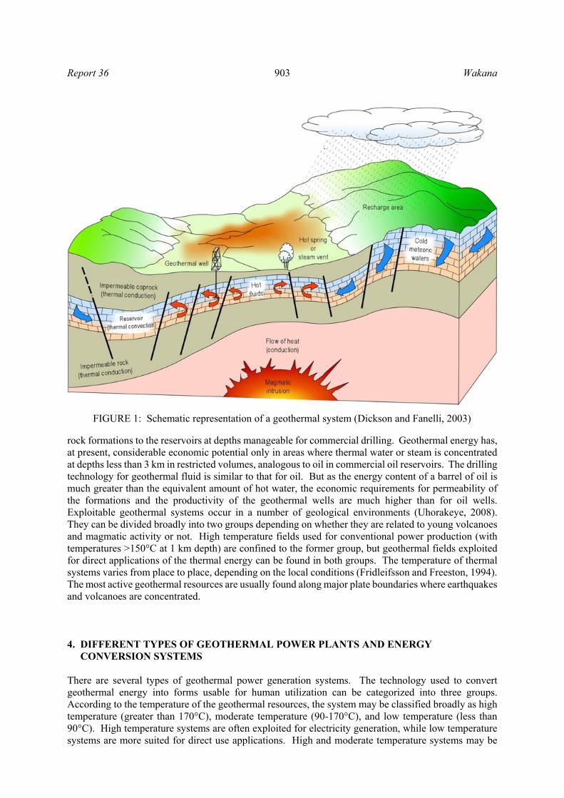
Geothermal energy is energy that comes from deep within the earth (Figure 1). Radioactive elements within the earth experience ongoing decay and release heat with a very high temperature. The high temperature heat is constantly released to space through a thick layer of rock. This heat flow produces energy called “geothermal energy” and is generated by a temperature difference between deeper hotter zones and shallower colder zones. Geothermal resources are characterized by features such as volcanoes, hot springs, geysers, and fumaroles. Most however, cannot be seen as they are deep underground. There may be no clues above ground that a geothermal reservoir is present. Geologists use different methods to find geothermal reservoirs. The only way to be sure there is a reservoir is to drill a well and test the temperature deep underground. At present, geothermal production wells are commonly 2 km deep, and rarely more than 3 km deep. The rocks have to be permeable in order to allow water to flow through and transfer heat from the hot

TABLE 1: The thirteen countries with highest geothermal

electricity production in 2010 (Fridleifsson, 2013)

Country GWh/Year

USA 16,603 Philippines 10,311 Indonesia 9,600 Mexico 7,047 Italy 5,520 Iceland 4,597 New Zealand 4,055 Japan 3,064 Kenya 1,430 El Salvador 1,422 Costa Rica 1,131

Report 36 903 Wakana

rock formations to the reservoirs at depths manageable for commercial drilling. Geothermal energy has, at present, considerable economic potential only in areas where thermal water or steam is concentrated at depths less than 3 km in restricted volumes, analogous to oil in commercial oil reservoirs. The drilling technology for geothermal fluid is similar to that for oil. But as the energy content of a barrel of oil is much greater than the equivalent amount of hot water, the economic requirements for permeability of the formations and the productivity of the geothermal wells are much higher than for oil wells. Exploitable geothermal systems occur in a number of geological environments (Uhorakeye, 2008). They can be divided broadly into two groups depending on whether they are related to young volcanoes and magmatic activity or not. High temperature fields used for conventional power production (with temperatures >150°C at 1 km depth) are confined to the former group, but geothermal fields exploited for direct applications of the thermal energy can be found in both groups. The temperature of thermal systems varies from place to place, depending on the local conditions (Fridleifsson and Freeston, 1994). The most active geothermal resources are usually found along major plate boundaries where earthquakes and volcanoes are concentrated. 4. DIFFERENT TYPES OF GEOTHERMAL POWER PLANTS AND ENERGY CONVERSION SYSTEMS There are several types of geothermal power generation systems. The technology used to convert geothermal energy into forms usable for human utilization can be categorized into three groups. According to the temperature of the geothermal resources, the system may be classified broadly as high temperature (greater than 170°C), moderate temperature (90-170°C), and low temperature (less than 90°C). High temperature systems are often exploited for electricity generation, while low temperature systems are more suited for direct use applications. High and moderate temperature systems may be

FIGURE 1: Schematic representation of a geothermal system (Dickson and Fanelli, 2003)


used for both electricity generation and direct use applications (Geoscience Australia and ABARE, 2010). The technology required to tap a geothermal system is determined by its temperature. For low to moderate temperature systems (<170°C), the electricity is often generated using “binary or ORC technology”. The geothermal fluids are transported to the surface in the production wells and the produced water is then piped to a power plant. The geothermal water flows through a heat exchanger, which causes the vaporization of the organic fluid. The cooled brine is re-injected in the injection well and the vapour drives a turbine which produces electricity. The expanded vapour is condensed in the condenser and pressurized again with the condensate pump to complete the cycle (Smeets, 2012). For a high-temperature system (>170°C), electricity is most often produced by passing the geothermal steam directly through a condensing steam turbine. The geothermal fluid from a reservoir reaches the surface as a mixture of steam and brine, due to boiling of the fluid. The steam is then separated from the brine, either by a cyclone effect in a vertical separator or by gravity in a horizontal separator. The dry steam is directed to a turbine which is connected to a generator to generate electricity, while the separated brine is piped back into the reservoir through reinjection wells. The power generation is called single flash (Nugroho, 2011). If the geothermal fluid from the well is at high pressures, double flash configuration is possible. In double flash configuration the geothermal fluid is first separate from the brine in high pressure separator, then second flashing of the brine is possible from the first separator. The resulting high pressure steam is directed to a high pressure turbine and the separated brine, which still contains reasonably high enthalpy, is throttled and directed to the low pressure separator for additional steam production. Steam from the high pressure turbine is mixed with the steam from the low pressure separator and then directed to the low pressure turbine to generate extra power. The brine from a low pressure separator is piped to the reinjection wells (Nugroho, 2011). Different combinations of cycles can be made in order to maximise the output power from a system. Among these are: binary cycle with a single-flash cycle using a back pressure turbine, a single flash using a condensing turbine and a binary cycle and a single flash back pressure cycle, a binary cycle utilizing separated brine and a binary cycle utilizing the exhaust steam from the back pressure unit, etc. (Nugroho, 2011). 5. OVERVIEW OF THE GEOTHERMAL RESOURCE IN BURUNDI

The East Africa Rift System (EARS) is known as one of the major tectonic structures of the earth where the heat energy of the interior of the earth escapes to the surface. This energy flow takes place in the form of volcanic eruptions, earthquakes and the upward transport of heat by hot springs and natural vapour emissions. The estimated geothermal energy resource potential in the East Africa Rift System is more than 15,000 MWe (Teklemariam, 2012). Geothermal resource manifestations exist in many locations in the western part of Burundi. This western part of Burundi is connected to the East Africa Rift system (EARS) in the western branch (Figure 2). Many reports have been made in Burundi, describing the geothermal manifestation since 1878 by Stanley, e.g. in 1968, 1972, and 1981, and by UNDP. Some reports described the locations and the chemical analyses. By request of the Ministry of Public Works, Energy and Mines of Burundi in 1981, the Icelandic International Development Agency carried out a reconnaissance survey in 1982. During the reconnaissance mission of 1982, Ármannsson and Gíslason visited 14 geothermal sites, comprising all known geothermal locations in the country. These are all sites of hot springs with temperatures ranging from near ambient (22°C) to 63°C. All the geothermal sites are located in the


western part of the country (Figure 3); six (6) are located within the western branch of the Eastern Africa Rift valley. The hottest springs are all located in the Rift Valley and the three (3) hottest ones, Ruhwa, Gasenyi and Ruhanga, are located in the Rusizi Valley, north of Lake Tanganyika. Of the remaining eight, seven are located less than 40 km east of the Rift Valley and one, Mashuha, is located some 60 km east of the Valley (Fridriksson et al., 2012). 5.1 Geological context

The Rift System may be divided into two main branches, i.e. the eastern branch and the western branch. The western branch runs over a distance of 2100 km, from Lake Albert in the north to Lake Malawi in the south (Figure 4). The central segment of the rift, trending NW-SE, includes Lake Tanganyika (773 m a.s.l.) with a surface area of 32,600 km2, about 650 km long and up to 70 km wide. The maximum thickness of the sediment fill is 4-5 km in the Tanganyika basin. The sediments started to accumulate in Miocene or early Pliocene. The Tanganyika basin is divided on the western side by normal faults with a curved trace (Fridriksson et al., 2012), and into several asymmetric sub-basins by NW-striking faults. On the northern part of Lake Tanganyika, these faults are accompanied by geothermal activity. In the western branch of the East Africa Rift Valley, volcanic activity is more widespread than in the eastern branch. In the adjacent province of the neighbouring countries, such as DRC and Rwanda, the geochronological and petrological data suggest that volcanism associated with the western rift began ~11 Ma ago in the Virunga region, north of Lake Kivu, ~10 Ma ago in the Bukavu Province, south of Kivu, and 9 Ma ago in the Rungwe region, east of Lake Tanganyika. In each of these three provinces, volcanism began before the initial subsidence of the local sedimentary basins. However, in the Tanganyika basin or Burundi, there is no related subaerial volcanism, but there are some indications of under plating of magma below the Tanganyika basin (Fridriksson et al., 2012). Tholeiites, which originated in the Bukavu Province, south Kivu, are found in the north-westernmost part of Burundi, on the borders of Rwanda and DRC (Ármannsson and Gíslason, 1983).

FIGURE 2: Main structures of the EARS; main faults are marked with black lines

FIGURE 3: Geothermal sites in Burundi and the main tectonic structures


The map in Figure 4 indicates that the lavas entered the NW tip of Burundi. The Burundian bedrock is mostly composed of Precambrian formation and complexes. Dominant rock types are quartzite, gneiss, granite, dolomite, schist, sandstone and conglomerate. The Rusizi valley is filled with thick sequences of alluvium formed during the Holocene. Sediments from Pleistocene, mostly lithified sandstone and conglomerates, are characteristic of the area east of the Rusizi valley, overlying Precambrian formations. Tertiary tholeiitic and alkali lavas are found in NW Burundi (covering some 30 km2), originating from the volcanic zone of south Kivu in Rwanda. The age of the lava flows is estimated to be 6-8 Ma (Ármannsson and Gíslason, 1983). According to several researchers, the hot springs in NW Burundi do not seem to be directly associated with the Cenozoic basalts found in that area, but they infer that under plating of magma might be an important process beneath the Tanganyika Rift (Fridriksson et al., 2012) on the western shore of Lake Tanganyika, along the N-S major faults with NW-SE trending faults (Fridriksson et al., 2012). The geothermal systems within the sediments of the

Tanganyika Rift in Rusizi are generally characterized by low porosity and permeability (Ármannsson and Gíslason, 1983). 5.2 Geochemical analytical context

The highest source temperatures were suggested to be in the Rift Valley according to the Icelandic GeoSurvey reports produced in 1983 and 2012. Three sites of highest temperatures were estimated at locations in the Rusizi valley. All discharges in the Rusizi Valley were carbon dioxide rich. This could indicate the presence of a powerful heat source. The high carbon dioxide concentrations lead to super saturation with respect to calcium carbonate, in some cases, so that care would have to be exercised in avoiding calcium carbonate deposition in the event of exploitation. The chemical compositions in Ruhwa are classified as CO2–rich Na-HCO3 waters and are very similar to the results of the Mashyuza samples in Rwanda. The chemical compositions are characteristic of all the geothermal resources in the Rusizi Valley in Burundi, i.e. Ruhwa, Ruhanga, Cibitoke and Gasenyi (Fridriksson et al., 2012). Using chemical geothermometers to assess the likely temperature in the reservoir, the highest was found in Ruhwa with 102°C, slightly lower than the 110°C observed for the 1983 sample. This temperature is low for electricity production with conventional flashing technology, but a binary unit is a possible option.

FIGURE 4: Distribution of Cenozoic lavas in the Kivu Province and neighbouring areas


6. GEOTHERMAL BINARY POWER PLANT DESIGN 6.1 Introduction The low to medium temperature sources are unusable for generating electricity with conventional methods. These resources are a water-dominated system and they cannot flash the steam for driving the turbine to generate power. In order to generate electricity from low-to-medium temperature sources and to increase the utilization of thermal resources by recovering waste heat, binary technologies have been developed. The binary plant technologies use a secondary working fluid. Intense research has been done on binary technologies and it shows promising results for converting low and medium temperature resources into electricity. The technology is still being developed to enhance the overall net conversion efficiency (Paci et al., 2009). Generally, there are two main types of binary cycles, the Organic Rankine Cycle (ORC) and the Kalina cycle. The ORC commonly uses hydrocarbons as the appropriate working fluid and Kalina uses a water-ammonia mixture (typically around 85-15 weight by percentage) (Kopunicova, 2009). The Kalina cycle achieves a thermodynamic efficiency (brine effectiveness) that is approximately 50% greater than that of standard binary Rankine plants (Dickson and Fanelli, 2003). The objectives of this design are:

To analyse the feasibility of a binary power plant with the parameter conditions of the Rusizi area, using an Organic Rankine Cycle; and

To compare a net power output (efficiency) by using an Organic Rankine cycle and a Kalina cycle.

6.2 Technical overview of binary geothermal power plants 6.2.1 Organic Rankine Cycle power plant Binary cycle geothermal power plants are close in thermodynamic principle to conventional fossil or nuclear plants in that the working fluid is in a closed cycle. The binary working fluid is contained completely within pipes, heat exchangers and the turbine, so that it never comes in chemical or physical contact with the environment (DiPippo, 2008). A binary system has two fluid streams: first is the heat exchange of the geothermal fluid where the working fluid of the ORC absorbs heat from the geothermal fluid via the heat exchanger; the second is the ORC working cycle. These two fluid streams are separated and the heat transfer takes place through the heat exchangers; normally, shell-and-tube heat exchangers are applied. The simple organic Rankine Cycle power plant follows the scheme shown in Figure 5. The organic fluid receives heat from the geothermal fluid in a heat exchanger (5-6) and finally is vaporized (6-1) before entering the turbine to produce mechanical work and eventually electricity in the generator. After isobaric heat addition, which occurs between states 5 and 1, high-pressure vapour is expanded in the turbine (1-2). After expansion, the organic fluid is sent to a condenser where it is cooled and condensed (2-4) and then pumped (4-5) again in a closed circuit to be vaporized again. Binary power plants usually have a separate cooling medium that can be fresh water or air. Air cooled condensers are usually a solution for power plants with no fresh water availability. After the heat from the geothermal fluid has been utilized in the heat exchangers the temperature of it is lower and it is re-injected in a injection well for recharge to the reservoir.


6.2.2 Parameters of the Organic Rankine Cycle Parameters of the preheater and evaporator: The preheater and evaporator are components that are used to transfer heat from the geothermal fluid to the working fluid. These component are often referred to as heat exchangers and in some cases these two components are one unit. In this case, the preheater and evaporator are separated. The preheater heats the working fluid before it enters the evaporator. When the boiling point is approached, the organic fluid is

transferred to the evaporator to evaporate before being sent to the turbine. The heat losses through the heat exchanger to the environment are neglected and the total amount of heat added to the organic fluid is equal to the heat extracted from the geothermal fluid. This transfer is described below:

(1)

(2)

where mgeo = Mass flow of geothermal fluid (kg/s); mwf = Mass flow of organic fluid (kg/s); ha = Enthalpy of geothermal fluid entering the evaporator (kJ/kg); hc = Enthalpy of geothermal fluid leaving the preheater (kJ/kg); h1 = Enthalpy of organic fluid leaving the evaporator (kJ/kg);

h5 = Enthalpy of organic fluid entering the evaporator (kJ/kg); wf = Organic fluid; and geo = Geothermal fluid.

Hence, the thermodynamic heat balance is:

(3)

And in a case where the geothermal fluid contains low dissolved gases and solids, the previous equation becomes:

(4)

where cp = Specific heat capacity of water at constant pressure (kJ/kg°C); Ta = Temperature of geothermal fluid entering the evaporator (°C); and

Tc = Temperature of geothermal fluid leaving the preheater (°C). Considering the constant geothermal fluid heat capacity, the energy balance in the evaporator and the preheater can be described by the following equations

For evaporator: (5)

For preheater: (6)

FIGURE 5: Simplified schematic of a basic ORC power plant


where Tb = Temperature of geothermal fluid between evaporator and preheater (°C); and h6 = Enthalpy of geothermal fluid between evaporator and preheater (kJ/kg). In this design, the heat exchanger’s function is demonstrated in the temperature – heat transfer, or T-Q, diagram (Figure 6). The abscissa represents the total amount of heat that is passed from the geothermal fluid to the organic fluid. The preheater provides sufficient heat to raise the organic fluid to its boiling point (1-2). The evaporation occurs from states 6-1 (referring to Figure 5) along an isotherm for a pure organic fluid (2-3 in Figure 6). The place in the heat exchanger where the geothermal fluid and the organic fluid experience the minimum temperature difference is called the pinch point, and the value of that difference is designated the pinch point temperature difference Tpp (DiPippo, 2008). The pinch point location and the value of the pinch point temperature difference are two major parameters influencing the performance of the heat exchanger. The pinch point temperature is generally known from the heat exchanger manufacturer’s specifications. The total amount of heat transferred in the heat exchanger is given by the following equation (DiPippo, 2008):

∙ ∙ (7)

Where U = Overall heat transfer coefficient (W/m2K); A = Total heat transfer area (m2); and LMTD = Logarithmic mean temperature difference (K). LMTD can be expressed by the following equation:

, , , ,, ,

, ,

(8)

where Thot,in = Temperature of geothermal fluid at heat exchanger inlet (K or °C); Tcold,out = Temperature of geothermal fluid at heat exchanger outlet (K or °C); Thot,out = Temperature of organic fluid at heat exchanger outlet (K or °C); and Tcold,in = Temperature of organic fluid at heat exchanger inlet (K or °C).

Parameters of the turbine and generator: The turbine is a device that converts the thermal energy from the organic fluid into electrical energy through the generator. The pressurized vapour steam of organic fluid expands in the turbine and leads to rotation of the rotor. The rotor is connected to a generator which changes rotational kinetic energy into electricity. The expansion process in the turbine is considered adiabatic and steady state of the operation is assumed. The efficiency of the turbine (th) is isentropic and is given by the manufacturer. The power generated by the turbine can be calculated by the following equation in accordance with Figure 5 (DiPippo, R., 2008):

(9)

(10)

where h1 = Enthalpy of organic fluid at turbine inlet (kJ/kg);

FIGURE 6: Preheater and evaporator temperature distribution (modified from DiPippo, R., 2008)


h2 = Enthalpy of organic fluid at turbine outlet (kJ/kg); h2s = Enthalpy of organic fluid at turbine outlet assuming isentropic expansion (kJ/kg); th = Efficiency of the turbine.

Parameters of the condenser: The condenser is a heat exchanger between the hot vapour from the turbine and the cooling medium (either water or air) of the cycle. The calculation of the condenser is roughly the same in both cases. The working fluid comes from the turbine to the inlet of the condenser through point 2 (Figure 5) and from the outlet of the condenser at point 4. The cooling fluid comes from the cooling system for entry into the condenser at point C1 and from the outlet condenser at point C2, as shown in Figure 7. A good cooling system improves the net power of the plant and can cool the working fluid to an optimal pressure and temperature. It also controls the reinjection temperature of the geothermal fluid. There are two types of cooling systems (Khaireh, 2012). Wet cooling system: The wet cooling system uses both water and air (Figure 7). The system is composed of a surface condenser which condenses the working fluid before entering the pump. While transferring heat to the cooling water, the working fluid changes phases and then goes directly to the pump. The main technology used in geothermal plants is mechanical draft induced with a fan instead of natural draft. There are two main tower configurations available, indicating the direction of the air flow in relation to the water flow:

Counter flow; and Cross flow.

The cold water from the cooling system is used to dissipate heat stored in the condenser. After going through the exchanger, the hot water from the condenser passes through a cooling tower and is cooled down by a fan, using outside air. A supply of make-up water (C3) is needed to compensate for evaporation losses. A wet cooling system is commonly used in many geothermal plants for high efficiency, but presents some disadvantages, like the large amount of water needed, water vapour plumes and also some corrosion in the fan due to the chemistry. Most geothermal plants use an induced drafted fan on top of the tower, for a better cooling process. The energy balance of the wet cooling system requires complex equations due to the numerous parameters involved. It takes account of the air entering and leaving, as well as the water entering and leaving the condenser and the make-up water supply. These equations are expressed below. Mass balance for dry air:

(11)

where main = Mass flow of cold air entering cooling system (kg/s); maout = Mass flow of hot air leaving cooling system (kg/s); and mair = Mass flow of air used by cooling system (kg/s).

FIGURE 7: Wet cooling system (modified from Khaireh, 2012)

2

4

C1

C2

C3

Air outlet flow

Air inlet flow

Water feeding pond


Mass balance for water and the vapour content in the air stream:

(12)

where mvin = Mass flow of water vapour entering cooling system (kg/s); mvout = Mass flow of water vapour leaving cooling system (kg/s); mc1 = Mass flow of water entering the condenser (kg/s);

mc2 = Mass flow of water leaving the condenser (kg/s); and mc3 = Mass flow of makeup water entering the cooling system (kg/s).

The relationships between the dry air and the vapour stream entering and leaving are:

(13)

(14)

where out = Specific humidity of cold air entering the cooling system (kg water/kg dry air); and in = Specific humidity of hot air leaving the cooling system (kg water/kg dry air).

The equation for energy balance, taking Equation 12 into consideration, is:

(15)

where hin = Enthalpy of dry air entering the cooling system (kJ/kg); hout = Enthalpy of dry air leaving the cooling system (kJ/kg); hvin = Enthalpy of water vapour entering the cooling system (kJ/kg); hvout = Enthalpy of water vapour leaving the cooling system (kJ/kg); hc1 = Enthalpy of cold water leaving the cooling tower system (kJ/kg); hc2 = Enthalpy of hot water entering the cooling tower system (kJ/kg); and hc3 = Enthalpy of makeup water (kJ/kg). For a unit of dry air, Equation 15 becomes:

mm

∗ h hmm

∗ hmm

∗ hmm

∗ hmm

∗ h h (16)

Using Equations 13 and 14, Equation 16 becomes:

∗mm

∗ ∗ ∗ ∗ (17)

∗

mm

∗ ∗ ∗ ∗ (18)

The inflow of dry air is unchanged in the tower, but there are water losses due to evaporation, as well as drift losses in droplets carried out of the cooling tower with exhaust air. To prevent scaling and to avoid an accumulation of impurities, an amount of water is blown out from the basin. The mass flow of evaporation, me, is given (El-Wakil, 1984) by:

(19)

The drift losses, mdrift, can be estimated by the following equation (Perry and Green, 2008):

0.0002 (20)

And the blow down for mass flow is calculated by the formula (Perry and Green, 2008):

11

(21)

where mbl = Blowdown consistent unit (kg/s); and cycle = Ratio of dissolved solids in the recirculation water to dissolved solids in make-up

= water, normal range between 3 to 5 cycles.


Therefore, the make-up water required is found by the equation:

(22)

Dry cooling system: The dry cooling system uses air to condense steam from the turbine by forcing ambient air over a bundle of finned tubes containing the steam inside. It is often used where a water supply is not available near the power plant. Mostly, in geothermal plants, the dry air cooling system is a mechanical draft type using fans with motors driven by electrical power. There are two main configuration of the placement of fan in mechanical dry cooling system:

1. The induced draft configuration has is a mechanical fanon top of the tower. The fan pulls air over the tube bundles and blows it away reducing risk of recirculation. High power is needed if the ambient temperature is high, due to low inlet air velocities.

2. The forced draft configuration has a mechanical fan on the bottom of the tower, to force air into circulating over the bundle tubes. Air is circulated uniformly in the tower due to the low discharge air velocities from the bundle tube and has more of recirculating the air than induced draft. The forced draft configuration is more impacted by cold climatic conditions.

The dry cooling system is very sensitive to ambient temperature variations, which directly affect the output of the power plant. Unlike with wet cooling systems, the need for a make-up water supply is eliminated as are water freezing problems, and water vapour plumes. The maintenance and operation requirements and costs are low due to fewer components being used. The energy balance in the dry cooling system condenser, Figure 8, is represented by the following equation:

, ∆ (23)

where T is the difference between the air temperature entering and leaving the cooling system. Equation 23 can be expressed as:

, (24)

where mwf = Mass flow of working fluid (kg/s); mair = Mass flow of air flowing inside the condenser (kg/s); cp,air = Specific heat capacity of air (kJ/kg K); Tc1 = Temperature of the ambient air entering the cooling system (°C); and Tc2 = Temperature of the ambient air leaving the cooling system (°C). The power used by the fans to move air through the cooling system is found by the following equations:

∆ ,

(25)

,

(26)

, ,

(27)

where wfan = Mechanical work of fan; va = Volume flow of air; P = Static head of fan; fan,motor = Efficiency of fan motor; ma = Mass flow of air; and a,out = Density of air.


The feed pump: The feed pump is used increase the pressure of the working fluid and push it from the condenser to the preheater. The process of pumping is assumed to be isentropic. The power used by the feed pump is expressed with the following equation:

(28)

where Wfp = Work of the feed pump (kW); h5s = Enthalpy of the working fluid assuming isentropic process; and p = Isentropic pump efficiency. The net power output and thermal efficiency of the binary cycle: The net power output depends upon the components of the power plant, like preheater and evaporator efficiency. Another parameter to be considered is the cooling system and circulation pump which consume a great fraction of the generated power. The circulation pumps use generally between 2 and 10% of the gross power of the plant and the cooling tower fans can vary between 10 and more than 30% of the gross power (Franco and Villani, 2009). The relationships below give the net power output of the binary power plant:

, (29)

where Wnet = Net power output of power plant; Wturbine = Power produced by turbine; Wpump = Power used by all pumps in cycle; and Pfan,motor = Power used by cooling fans. The thermal efficiency is found by using the first law of thermodynamics; here the division of the work produced by the turbine and the heat extracted from the geothermal fluid in the preheater and evaporator. The heat extracted from the heat exchanger (preheater and evaporator) is given by Equation 2, and the thermal efficiency of the cycle is given by the following equation:

(30)

Working fluid selection: The working fluid needs to be carefully selected, based on the geothermal brine temperature and the fluid’s thermodynamic properties. The working fluid has great influence on the performance of the power plant. There are many working fluids, but the choice must have a lower boiling point than water, and have no negative impacts on health, safety and the environment (DiPippo, 2008). Hydrocarbons and refrigerants are the most common fluids used. In this study, three hydrocarbons, one refrigerant and a mixture of ammonia-water are considered, as shown in Table 2, to optimize the efficiency and net power output of a binary power plant.

TABLE 2: Properties of the working fluid

Fluid Formula Critical

temperature Tc (°C)

Critical pressure Pc (bar)

Molecular weight,

M (g/mol) Isobutane (CH3)3CH 135 36.85 58.12 Isopentane C5H12 187.20 33.78 72.149 Propane C3H8 96.6 42.36 44.10 R134a CF3-CH2F 101 40.59 102

Scaling prevention: Different types of scales are found in various geothermal areas. The major scaling species in geothermal brine typically include calcium, silica and sulphide compounds. Calcium compounds frequently


encountered are calcium carbonate and calcium silicate. Metal silicate and metal sulphide scales are often observed in high temperature resources. Silica can present even more difficulties, as it will form an amorphous silica scale that is not associated with other cations. Calcium carbonate scale frequently causes operational problems in the brine handling system. It typically forms as a result of the decrease of solubility of CO2 in the liquid phase. The solubility of CO2 decreases any time a pressure drop occurs and corresponds with increasing pH (Stapleton and Weres, 2011). At elevated temperatures, even small amounts of calcium in the brine will precipitate with pH increase. Calcium carbonate scale can form in production wells, plant vessels and equipment, and injection lines and wells. Silica related scale is one of the most difficult scales occurring in geothermal operation. Silica is found essentially in all geothermal brine and its concentration is directly proportional to the temperature of the brine. As brine flows through the well to the surface, the pressure drops and the temperature of the brine decreases. This entails that silica solubility decreases correspondingly and the brine phase becomes over saturated. Under these conditions, silica precipitates as either amorphous silica or it will react with available cations (e.g. Fe, Mg, Ca, Zn) and form co-precipitated silica deposits. These deposits are extremely tenacious and can occur throughout the production field, plant and injection systems. Effective scale prevention in geothermal operations is often critical to the success of a project. The scale prevention methods are related to site-specific conditions in the field. These conditions dictate the type of scale prevention method that will be feasible. Calcium carbonate scaling may be prevented by:

a) Acting on carbon dioxide partial pressure; b) Acting on the pH of the solution; and c) Using chemical additives (scale inhibitors).

Pressure and temperature manipulations of the geothermal fluid can be achieved quite easily by pumping a geothermal well instead of relying on its natural flow. Adding HCl to the geothermal fluid in order to decrease the pH below a certain value at which no calcite scaling can form is technically possible but expensive. The utilization of scale inhibitors is the most common and promising method of combating scaling problems. The main problem is to select the most suitable inhibitor among the hundreds of different chemicals on the market (Stapleton and Weres, 2011). Thermodynamic modelling of an Organic Rankine Cycle: In this study, the model presented in Figure 8 is a simple binary cycle using an organic working fluid, such as isopentane, isobutane, propane or R134a. The working cycle components are the preheater, evaporator, turbine, condenser, and pump. The condenser is cooled by a dry cooling system. The cooling system uses a fan and motor to supply and remove air. The cooling system was chosen with regard to the Rusizi area conditions. In this area, there are two rivers, Rusizi River and Ruhwa River. These two rivers are shared by the Democratic Republic of Congo and Rwanda. The use of these rivers required an agreement between these countries. The geothermal water is pumped from a well in order to pressurize it. Using Engineering Equation Solver (EES) software, a thermodynamic model of the binary plant cycle was developed for all working fluids and the parameters of the cycle were analysed. The EES program is given in Appendix I. The objectives were optimization of the efficiencies of different working fluids and obtaining the net power output with a temperature range of 90-140°C and a geothermal flow rate of 20-80 kg/s. The ranges used refer to the reconnaissance study report of the geothermal areas in Burundi, produced in September 2012. These ranges were estimated using the geothermometer analysis method. Many input data were


estimated during the development of the thermodynamic cycle of the binary plant, because of the lack of sufficient data being available from the field. Table 3 shows the assumptions that were made. Optimization of turbine inlet pressure of working fluid cycle: The optimal design of a binary geothermal power plant can be considered as a multi-objective, multi-variable constrained optimization problem. Three main temperatures can be considered as constraints, i.e. the geo-thermal fluid, rejection, and ambient temperatures. The whole optimization problem can be reformulated into manageable sized sub-problems. The results from the high optimization level represent the input data for the detailed design. The effects of the optimum component design (pressure losses, pumping power) are iterated at the system level (Franco and Villani, 2009).

TABLE 3: Design parameters assumed for the binary cycle power plant In this study, the turbine inlet optimum pressure required for every working fluid was considered for a temperature resource in the range between 90 and 140°C; the pressure was optimized to obtain a good output from the binary power plant design. The turbine inlet pressure plays an important role in producing mechanical force for driving a generator. The net power output was considered a parameter in this optimization as was the reinjection temperature, in order to prevent possible calcite carbonate

Parameters UnitMinimum

value Maximum

value Mass flow rate of geofluid kg/s 20 80 Temperature of geofluid from the well °C 90 140 Pressure of geofluid from the well bar 30 Reinjection temperature °C 70 Ambient temperature of Rusizi area (Ndayirukiye, 1986) °C 30 Turbine efficiency % 85 Feed pump efficiency % 75 Fan efficiency % 65 Atmospheric pressure bar 1.02 Relative humidity (Ndayirukiye, 1986) % 70 Pinch point of vaporizer °C 5 Air temperature leaving the cooling system assumed equal to ambient temperature plus 12°C

°C 42

Working fluids: isobutane, isopentane, propane and R134a kg/s Vaporizer pressure bar Optimized OptimizedTemperature of condenser oC 45

1

2

3

4

5b

c

a

Evaporator

Brine pump

Feed pump

Preheater

Condenser

Air cooling system

Turbine

Generator

FIGURE 8: Binary cycle with air cooling system


scaling that could occur during operation. The optimization of the inlet turbine pressure was achieved by using a computer code. EES software was helpful in creating the code to resolve thermodynamic problems. It was used in this study to optimize different parameters of the design cycle, including the pressure inlet into the turbine for the temperature range 90°C and 140°C, with respect to the reinjection temperature while other parameters where constant. The optimization was done for all working fluids and analysed to find the highest work output. The behaviour and work output of the working fluid at different pressures allowed the selection of the optimum pressure. Figure 9 shows the optimum pressure for each working fluid at different temperatures.

FIGURE 9: Power plant output with turbine inlet pressure

After optimization, it was observed that some working fluids showed a different optimal pressure at different temperatures or the same optimal pressure in a certain temperature range. One working fluid, R134a, gave an optimal output at the same pressure throughout the temperature range considered, and needs high pressure to generate an optimal output. A summary of the results of different optimum pressures for all working fluids at the various temperatures considered is shown in Tables 4-7.

10 15 20 25 30 35 40 450

10

20

30

40

50

60

70

80

90

100

Turbine inlet pressure [bar]

Sp

ec

ific

po

we

r o

utp

ut

[kW

/(k

g/s

)] Isopentane 120oCIsopentane 120oC

Isopentane 140oCIsopentane 140oC



Isopentane 100oCIsopentane 100oCIsopentane 90oCIsopentane 90oC

Isopentane

10 15 20 25 30 35 40 450

10

20

30

40

50

60

70

80

90

100


Sp

ec

ific

po

we

r o

utp

ut

[kW

/(k

g/s

)]Isobutane 90oCIsobutane 90oCIsobutane 100oCIsobutane 100oCIsobutane 110oCIsobutane 110oCIsobutane 120oCIsobutane 120oC

Isobutane 130oCIsobutane 130oC

Isobutane 140oCIsobutane 140oCIsobutane

10 15 20 25 30 35 40 450

10

20

30

40


Sp

ec

ific

po

we

r o

utp

ut

[KW

/(k

g/s

)]

Propane 140oCPropane 140oCPropane 130oCPropane 130oCPropane 120oCPropane 120oCPropane 110oCPropane 110oCPropane 100oCPropane 100oCPropane 90oCPropane 90oC

Propane

10 15 20 25 30 35 40 450

5

10

15

20

25

30

35

40

45


Sp

ec

ific

po

we

r o

utp

ut

[KW

/(k

g/s

)]

R134a 90oCR134a 90oCR134a 100oCR134a 100oCR134a 110oCR134a 110oCR134a 120oCR134a 120oCR134a 130oCR134a 130oC

R134a 140oCR134a 140oC R134a


Power plant performance analysis: The first and second law efficiencies are usually used to assess the performance of binary power plants. These two parameters can help to compare the various available combinations of the source, rejection and condensation temperatures, and give indications about the specific power of the plant. Another important parameter to be considered is the mass flow rate used to generate a fixed power output. In this study, the thermodynamic parameters of the binary model cycle were developed and the EES program was used to estimate the parameter values of a model binary cycle. Knowing the pressure of the turbine inlet, the temperature of the geothermal resource, the ambient temperature, the reinjection temperature and the condenser temperature, other parameters could be calculated by EES. The calculation was done with a geothermal mass flow input of 1 kg/s as the heat source. The reinjection temperature used in this study was fixed at 70°C, considering the low enthalpy of the geothermal resource according to Alessandro and Marco Villani and the September 2012 reconnaissance study report of the geothermal resource in the Rusizi Valley. For a geothermal field that has temperatures between 110 and 160°C, it is difficult to use rejection temperatures lower than 70-80°C; the latter temperature is a crucial parameter in plant design (Franco and Villani, 2009). The condenser temperature was fixed at 45°C because the ambient temperature is very high, with an average of 30°C. Results of the analyses for a binary power plant model for all working fluids chosen are presented in Tables 4 to 7. The performance results are given as the exergy efficiency value as a function of temperature. The exergy efficiency, using the second law of thermodynamics, assesses the extraction of heat from a geothermal resource in regards to maximum theoretical work output. Figure 10 shows the behaviour of the exergy efficiency at different pressures and different temperatures of the geothermal resource. Among the working fluids used in this study, isopentane is better than the other working fluids, followed by isobutane. The first law efficiency and the exergy efficiencies with optained optimum turbine inlet pressure were calculated to assess the performance of different configurations. This assessment shows the losses in the cycle. The analysed results are illustrated in Tables 4-7. The exergy efficiency, the first law efficiency and the mass flow of the working fluid indicate the thermodynamic performance of a binary cycle. The objective is to extract more heat and gain the highest power output for the least cost. The investment is another parameter to be considered in binary power plant design. The results show that isopentane is better than the other working fluids tested. Figure 11 illustrates the behaviour of various working fluids used for an Organic Rankin cycle.

TABLE 4: Properties of isopentane

Tgeo (°C)

Tinj

(°C)

Power output (kW/kg·s) th exerg

mwf (kg/s)

90 70 12.57 0.14 0.50 0.17 100 70 22.7 0.17 0.68 0.255110 70 31.8 0.18 0.78 0.338120 70 42.6 0.20 0.85 0.424130 70 52.2 0.20 0.86 0.511140 70 62.0 0.20 0.87 0.599

TABLE 5: Properties of isobutane Tgeo

(°C)Tinj

(°C)Power output

(kW/kg·s) th exerg mwf

(kg/s)90 70 8.2 0.096 0.32 0.34

100 70 15.8 0.125 0.487 0.33 110 70 23.8 0.141 0.58 0.56 120 70 30.09 0.146 0.55 0.70 130 70 38.13 0.149 0.57 0.69 140 70 45.4 0.152 0.58 0.81

TABLE 6: Properties of propane

Tgeo (°C)

Tinj

(°C)

Power output (kW/kg·s) th exerg

mwf (kg/s)

90 70 3.8 0.045 0.15 0.28 100 70 9.07 0.071 0.27 0.43 110 70 14.05 0.083 0.34 0.60 120 70 18.7 0.088 0.37 0.76 130 70 23.4 0.091 0.38 0.91 140 70 28.3 0.094 0.39 1.078

TABLE 7: Properties of R134a

Tgeo

(°C)Tinj

(°C)Power output

(kW/kg·s) th exerg mwf

(kg/s)90 70 5.4 0.064 0.21 0.56

100 70 10.3 0.081 0.31 1.14 110 70 15.3 0.09 0.34 1.03 120 70 20.3 0.095 0.36 1.42 130 70 25.5 0.099 0.38 1.71 140 70 30.3 0.101 0.39 2.01


FIGURE 10: Exergy efficiency with turbine inlet pressure for different working fluids

10 15 20 25 30 35 40 45 50 550

0.2

0.4

0.6

0.8

1


ex

erg

y

exergyR134aexergyR134a

exergyPropaneexergyPropane

exergyIsobutaneexergyIsobutane

exergyIsopentaneexergyIsopentane

Exergy efficiency at 140°C

10 15 20 25 30 35 40 45 50 550

0.2

0.4

0.6

0.8

1


exer

gy






10 15 20 25 30 35 40 45 50 550

0.2

0.4

0.6

0.8

1


ex

erg

y






10 15 20 25 30 35 40 45 50 55

0.2

0.4

0.6

0.8

1

1.2


ex

erg

y






10 15 20 25 30 35 40 45 50 550

0.2

0.4

0.6

0.8

1

Turbine inlet pressure bar]

ex

erg

y






10 15 20 25 30 35 40 45 50 550

0.2

0.4

0.6

0.8

1

turbine inlet pressure [bar]

ex

erg

y







6.2.3 Investment cost estimation of Organic Rankine Cycle It is difficult to make accurate estimates of project costs at the conception stage. The cost estimates at this stage generally have a large margin of error. The level of accuracy of the cost estimates depends upon the information available. Capital cost of geothermal projects is very site and resource specific. The source temperature will determine the power conversion technology as well as the overall efficiency of the power system. Site accessibility and topography, local weather conditions, land type and ownership are additional parameters affecting the cost and the time required to bring the power plant online. This means that the costs of geothermal projects vary from site to site, as well as the cost of financing. In this study, the cost estimate is only a part of the total investment. The total cost considers the investment of the exploration phase, drilling wells and reservoir stimulation. The base costs of main equipment are estimated based on the experience of experts, as seen in Table 8. The costs are assumed to be thumb values, although best estimates should be obtained through vendor quotations. The parameters used to estimate the cost of purchased equipment include the surface area, power or capacity. To estimate the cost of equipment, calculations were done for one kilogram of geothermal water mass flow. The cost takes into consideration the area of the evaporator, the preheater, and the condenser, a feed pump, cooling tower and fan, turbine and well pump. The cost is shown in Figure 12 for the range of temperatures considered. The fixed capital investment is divided into two: direct cost (DC) and indirect cost (IC). The direct cost concerns: the purchased equipment cost (PED); purchased equipment installation (33% of PED); piping (35% of PED); instrumentation and controls (12% of PEC); electrical equipment and materials (13% of PEC); civil, structural and architectural work (21% of PEC); and service facilities (35% of PEC). The indirect costs include: engineering and supervision (8% DC); construction costs and contractor’s profile (15%); and 15% is added as a contingency to the DC and IC sums (Bejan et al., 1996). The first estimate of equipment cost, illustrated in Figure 12, showed the need for more investment for propane and R134a, compared to isopentane and isobutane. The highest cost was influenced by the biggest condenser area required for propane, followed by R134a and isobutane to lower the high temperature of the working fluid from the turbine to the low condenser temperature. Knowing the estimated cost of the equipment, one should be able to estimate other investment costs required for a binary power plant cycle. For estimation of the total cost of investment for a binary cycle power plant installation (Table 9), the assumptions above were used to calculate the fixed capital costs.

TABLE 8: Assumed thumb values for equipment costs

Equipment Unit sizeBase cost / unit size

(USD) Preheater m2 450 Evaporator m2 500 Condenser m2 600 Turbine kW 500 Pump kW 450 Motor kW 450

0

10000

20000

30000

40000

50000

60000

70000

90 100 110 120 130 140

CO

ST

IN

US

D

TEMPERATURE OF GEOFLUID [°C]

Total investment per kg/s of geofluid

Isopentane

Isobutane

Propane

R134a

FIGURE 12: Comparison of estimated equipment costs for the ORC at different temperatures with one kg/s of geothermal mass flow


TABLE 9: Total cost of ORC for 1 kg/s of geofluid in USD, evaluated for various temperatures of geofluid

6.2.4 Economic analysis of Organic Binary Cycle model Considering the price of electricity (0.18 USD/kWh in March 2012) (Ministry of Energy and Mining of Burundi, 2012) from REGIDESO which is responsible for the production and distribution of water and electricity in Burundi, the annual cost of energy was calculated, and ten years was considered the time needed for a return of investment. The cost of operation and maintenance was estimated as 6% of the annual revenue. Two scenarios assuming 10% and 15% interest rates were analysed. The baseline for the calculation used was the thermal design and optimization book (Bejan et al., 1996). The mass flow of the geothermal resources was estimated to be in the range of 20-80 kg/s. The results of the calculation are presented below; the following equation was used:

1 (31)

where F = Future value in n years; P = Present value that is equal to total cost of investment; i = Earning rate (%) in interest per year; and n = number of years for investment return.

Annual cost of energy = 0.18 USD/kWh * value of power * value hours per days * number of days per year. The annual revenue is the difference between the annual energy cost and the cost of maintenance and operation. In this study, tax depreciation was neglected. The results of the analysis are shown in Figure 13. The results show the behaviour for different temperatures in two scenarios with the same price charged by REGIDESO and with augmentation of the energy price. Isopentane was shown to be economical in all ranges of geothermal temperature in both scenarios. Isobutane was economical in the range between 100 and 140°C for an interest rate of 15% at REGIDESO prices. Propane and R134a showed an economical result in the range 120-140°C when the price was increased by 39%.

6.2.5 Kalina cycle power plant The first version of the Kalina cycle was invented and proposed by Eng. Alexander Kalina in 1980. A Kalina cycle is a modified organic cycle using a mixture of ammonia-water as a secondary working fluid in specific ratios and may be the preferred choice for geothermal resources with temperatures below 140°C (Oguz, 2011). Ammonia-water used as working fluid was the most preferred among several organic mixtures which yielded maximum geothermal water utilization. The technology of a Kalina cycle has developed over the last two decades; however, commercial marketing of the technique started only a few years ago (Lolos and Rogdakis, 2009). The innovative technology has undergone intense development, optimisation and large-scale demonstrations, based on the initial version, with significant power generation in the industrial world. The first Kalina cycle was constructed between 1991 and 1997 at Canoga Park, California, for demonstration purposes with a 6.5 MW installed capacity and ran for a total of 8600 hours. This period

Temperature (°C)

Isopentane (USD)

Isobutane (USD)

Propane (USD)

R134a (USD)

90 16,579 16,690 18,504 19,637 100 24,313 25,204 27,807 28,315 110 24,313 35,560 37,227 28,315 120 40,962 43,925 45,988 45,704 130 48,801 52,345 54,806 54,473 140 56,713 60,844 63,705 63,323


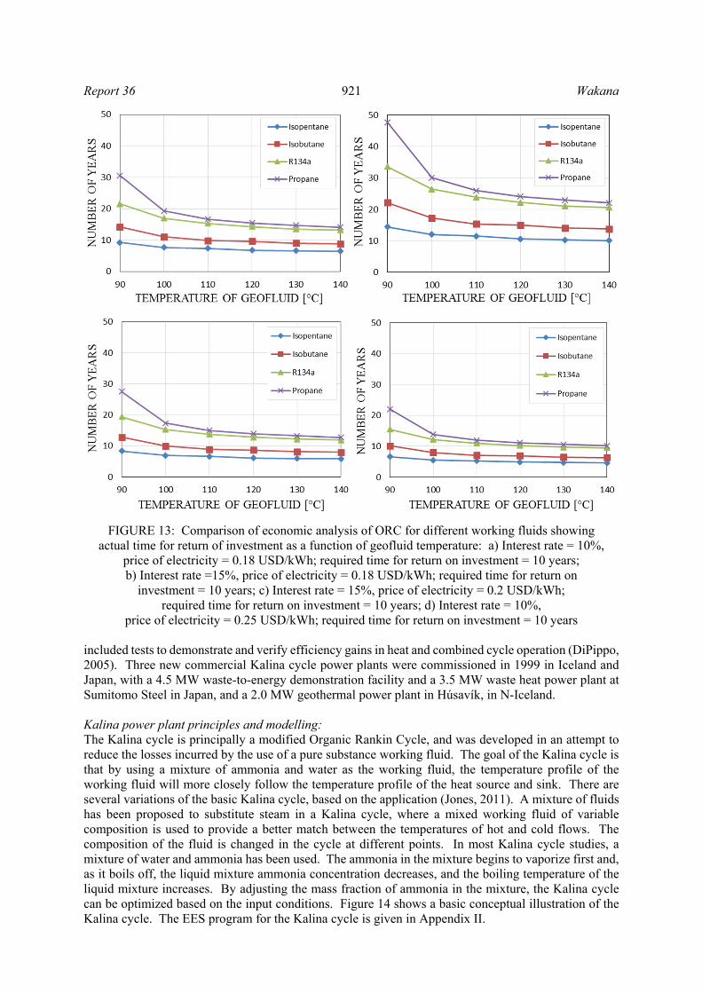
included tests to demonstrate and verify efficiency gains in heat and combined cycle operation (DiPippo, 2005). Three new commercial Kalina cycle power plants were commissioned in 1999 in Iceland and Japan, with a 4.5 MW waste-to-energy demonstration facility and a 3.5 MW waste heat power plant at Sumitomo Steel in Japan, and a 2.0 MW geothermal power plant in Húsavík, in N-Iceland. Kalina power plant principles and modelling: The Kalina cycle is principally a modified Organic Rankin Cycle, and was developed in an attempt to reduce the losses incurred by the use of a pure substance working fluid. The goal of the Kalina cycle is that by using a mixture of ammonia and water as the working fluid, the temperature profile of the working fluid will more closely follow the temperature profile of the heat source and sink. There are several variations of the basic Kalina cycle, based on the application (Jones, 2011). A mixture of fluids has been proposed to substitute steam in a Kalina cycle, where a mixed working fluid of variable composition is used to provide a better match between the temperatures of hot and cold flows. The composition of the fluid is changed in the cycle at different points. In most Kalina cycle studies, a mixture of water and ammonia has been used. The ammonia in the mixture begins to vaporize first and, as it boils off, the liquid mixture ammonia concentration decreases, and the boiling temperature of the liquid mixture increases. By adjusting the mass fraction of ammonia in the mixture, the Kalina cycle can be optimized based on the input conditions. Figure 14 shows a basic conceptual illustration of the Kalina cycle. The EES program for the Kalina cycle is given in Appendix II.

FIGURE 13: Comparison of economic analysis of ORC for different working fluids showing actual time for return of investment as a function of geofluid temperature: a) Interest rate = 10%,

price of electricity = 0.18 USD/kWh; required time for return on investment = 10 years; b) Interest rate =15%, price of electricity = 0.18 USD/kWh; required time for return on

investment = 10 years; c) Interest rate = 15%, price of electricity = 0.2 USD/kWh; required time for return on investment = 10 years; d) Interest rate = 10%,

price of electricity = 0.25 USD/kWh; required time for return on investment = 10 years


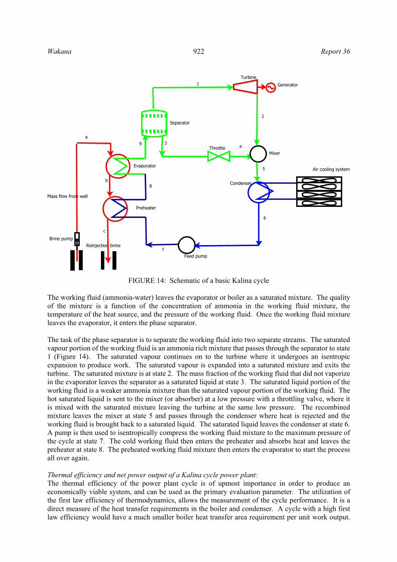
FIGURE 14: Schematic of a basic Kalina cycle The working fluid (ammonia-water) leaves the evaporator or boiler as a saturated mixture. The quality of the mixture is a function of the concentration of ammonia in the working fluid mixture, the temperature of the heat source, and the pressure of the working fluid. Once the working fluid mixture leaves the evaporator, it enters the phase separator. The task of the phase separator is to separate the working fluid into two separate streams. The saturated vapour portion of the working fluid is an ammonia rich mixture that passes through the separator to state 1 (Figure 14). The saturated vapour continues on to the turbine where it undergoes an isentropic expansion to produce work. The saturated vapour is expanded into a saturated mixture and exits the turbine. The saturated mixture is at state 2. The mass fraction of the working fluid that did not vaporize in the evaporator leaves the separator as a saturated liquid at state 3. The saturated liquid portion of the working fluid is a weaker ammonia mixture than the saturated vapour portion of the working fluid. The hot saturated liquid is sent to the mixer (or absorber) at a low pressure with a throttling valve, where it is mixed with the saturated mixture leaving the turbine at the same low pressure. The recombined mixture leaves the mixer at state 5 and passes through the condenser where heat is rejected and the working fluid is brought back to a saturated liquid. The saturated liquid leaves the condenser at state 6. A pump is then used to isentropically compress the working fluid mixture to the maximum pressure of the cycle at state 7. The cold working fluid then enters the preheater and absorbs heat and leaves the preheater at state 8. The preheated working fluid mixture then enters the evaporator to start the process all over again. Thermal efficiency and net power output of a Kalina cycle power plant: The thermal efficiency of the power plant cycle is of upmost importance in order to produce an economically viable system, and can be used as the primary evaluation parameter. The utilization of the first law efficiency of thermodynamics, allows the measurement of the cycle performance. It is a direct measure of the heat transfer requirements in the boiler and condenser. A cycle with a high first law efficiency would have a much smaller boiler heat transfer area requirement per unit work output.

1

2

34

5

6

7

8

9a

b

c

Turbine

Generator

MixerThrottle

Separator

Evaporator

Feed pump

Preheater

Reinjection brine

Mass flow from well

Air cooling system

Condenser

Brine pump


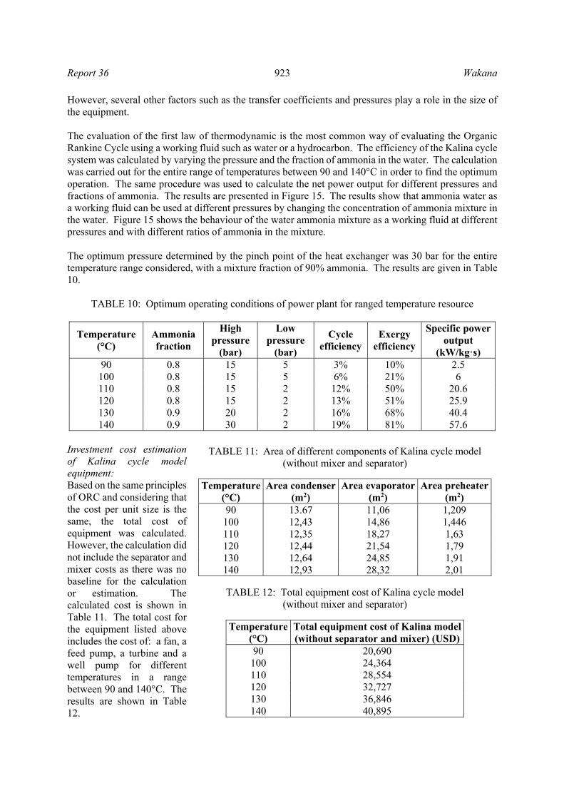
However, several other factors such as the transfer coefficients and pressures play a role in the size of the equipment. The evaluation of the first law of thermodynamic is the most common way of evaluating the Organic Rankine Cycle using a working fluid such as water or a hydrocarbon. The efficiency of the Kalina cycle system was calculated by varying the pressure and the fraction of ammonia in the water. The calculation was carried out for the entire range of temperatures between 90 and 140°C in order to find the optimum operation. The same procedure was used to calculate the net power output for different pressures and fractions of ammonia. The results are presented in Figure 15. The results show that ammonia water as a working fluid can be used at different pressures by changing the concentration of ammonia mixture in the water. Figure 15 shows the behaviour of the water ammonia mixture as a working fluid at different pressures and with different ratios of ammonia in the mixture.

The optimum pressure determined by the pinch point of the heat exchanger was 30 bar for the entire temperature range considered, with a mixture fraction of 90% ammonia. The results are given in Table 10.

TABLE 10: Optimum operating conditions of power plant for ranged temperature resource

Temperature (°C)

Ammonia fraction

High pressure

(bar)

Low pressure

(bar)

Cycle efficiency

Exergy efficiency

Specific power output

(kW/kg·s) 90 0.8 15 5 3% 10% 2.5

100 0.8 15 5 6% 21% 6 110 0.8 15 2 12% 50% 20.6 120 0.8 15 2 13% 51% 25.9 130 0.9 20 2 16% 68% 40.4 140 0.9 30 2 19% 81% 57.6

Investment cost estimation of Kalina cycle model equipment: Based on the same principles of ORC and considering that the cost per unit size is the same, the total cost of equipment was calculated. However, the calculation did not include the separator and mixer costs as there was no baseline for the calculation or estimation. The calculated cost is shown in Table 11. The total cost for the equipment listed above includes the cost of: a fan, a feed pump, a turbine and a well pump for different temperatures in a range between 90 and 140°C. The results are shown in Table 12.

TABLE 11: Area of different components of Kalina cycle model (without mixer and separator)

Temperature(°C)

Area condenser(m2)

Area evaporator (m2)

Area preheater(m2)

90 13.67 11,06 1,209 100 12,43 14,86 1,446 110 12,35 18,27 1,63 120 12,44 21,54 1,79 130 12,64 24,85 1,91 140 12,93 28,32 2,01

TABLE 12: Total equipment cost of Kalina cycle model

(without mixer and separator)

Temperature(°C)

Total equipment cost of Kalina model (without separator and mixer) (USD)

90 20,690 100 24,364 110 28,554 120 32,727 130 36,846 140 40,895


FIGURE 15: Comparison of net power output for different

pressure and fraction of ammonia in mixture

5 10 15 20 25 30 35 4010

20

30

40

50

60


Sp

ec

ific

po

we

r o

utp

ut[

kW

/(k

g/s

)]

X=0.9X=0.9

X=0.8X=0.8

X=0.7X=0.7

X=0.6X=0.6

X=0.5X=0.5

Specific power output at 140°C of geofluid

5 10 15 20 25 3010

15

20

25

30

35

40

45

Turbine inlet pressure [bar]S

pe

cif

ic p

ow

er

ou

tpu

t [k

W/(

kg

/s)]

X=0.9X=0.9

X=0.8X=0.8X=0.7X=0.7X=0.6X=0.6

X=0.5X=0.5

Specific power output at 130°C of geofluid

4 6 8 10 12 14 16 185

10

15

20

25

30

35


Sp

ec

ific

po

we

r o

utp

ut

[kW

/(k

g/s

)]

X=0.9X=0.9

X=0.8X=0.8

X=0.7X=0.7X=0.6X=0.6

X=0.5X=0.5

Specific power output at 120°C

4 6 8 10 12 14 16 18 205

10

15

20

25


Sp

ec

ific

po

we

r o

utp

ut

[kW

/(k

g/s

)]

X=0.9X=0.9X=0.8X=0.8X=0.7X=0.7X=0.6X=0.6X=0.5X=0.5


4 6 8 10 12 14 16 18 20 22 24 26 28 302

4

6

8

10

12

14


Sp

ec

ific

po

we

r o

utp

ut

[kW

/(k

g/s

)] X=0.9X=0.9X=0.8X=0.8X=0.7X=0.7X=0.6X=0.6X=0.5X=0.5


4 6 8 10 12 14 160

1

2

3

4

5

6


sp

ec

ific

po

we

r o

utp

ut

[kW

/(k

g/s

)]

X=0.7X=0.7X=0.8X=0.8

X=0.9X=0.9

X=0.6X=0.6

X=0.5X=0.5



7. COMPARISON OF ORGANIC RANKINE CYCLE AND KALINA CYCLE A simple model of a geothermal power plant was made to compare the thermodynamic performance of the two cycles. The main comparison consisted of power outputs and cycle efficiency. The two cycles utilized a secondary fluid for obtaining heat energy through a heat exchanger from a geothermal source. The difference between the ORC and Kalina cycle is in the working fluid and the equipment components. The Organic Rankine Cycle utilizes a hydrocarbon or refrigerant as a working fluid in a closed loop. The Kalina cycle has specific parameters due to its mixture of ammonia and water. The optimum turbine inlet pressure in the Kalina cycle depends on the ammonia fraction in the water-ammonia mixture and the temperature of geothermal fluid. These factors influence the optimum output and the heat extraction efficiency. The advantages of the Kalina cycle are being able to increase or decrease the power output by adjusting the fraction of ammonia in the mixture without changing any equipment. Theoretically, Kalina has a higher efficiency when the heat source stream has a finite heat capacity. But, ORC and Kalina are similar when the source is condensing steam (Valdimarsson, 2003). In this study, the ORC and Kalina cycles where analysed in regard to the first and second laws of efficiency. The performance of the Kalina cycle is similar to that of ORC. With temperatures below 100°C, the ORC cycle is a more favourable option than the Kalina Cycle. However, an increase in the temperature of the geothermal fluid leads to a increase in Kalina efficiency and power output. At 140°C, the efficiency and power output of Kalina are about the same as that of isopentane in the ORC, with the highest efficiency and power output. With the increase in geothermal fluid temperature, Kalina efficiency and power output might be higher than ORC at geothermal fluid temperatures above 140°C. That means that Kalina cycle performance at temperatures below 140°C has the same performance as ORC with the right working fluid. This result agrees with some authors who said that the Kalina cycle permits a gain in performance with respect to ORC. The adoption of the Kalina cycle, at least for low power levels and medium-high temperature thermal sources, does not seem to be justified by a gain in performance with respect to a properly optimized ORC. The gain is very small and is obtained with a complicated plant scheme, large surface heat exchangers and particularly high pressure resistant and non-corrosive materials, both expensive and unproven (Bombarda et al., 2010). The results on the performance of all the Organic Rankine Cycle working fluids used and the working fluid for the Kalina cycle are summarized in Tables 4-7 and 10. Considering the models, the Kalina cycle has many more components than the Organic Rankine Cycle and sometimes the setup is very complex. This increases the cost of a power plant. The comparison of equipment shows high costs for the Kalina cycle, without adding the cost of separator and mixer. The calculation was done using the same baseline for the ORC. Regarding power output for all ORC cycles used and for the Kalina cycle, isopentane gave the highest output followed by isobutane, R134a, propane and then the Kalina cycle at temperatures less than 100°C. But, between 100-120°C, the Kalina cycle produced higher power output than propane and R134a. At 130-140°C, output from the Kalina cycle increased quickly and gave the highest power output of the working fluids considered, except for isopentane. At 140°C, Kalina gave a power output near the power output given by isopentane. This means that if the temperature is higher than 140°C, the Kalina cycle would give higher power output than the isopentane. Looking at the energy input and power output in the modelled systems, the answer is clear. For temperatures lower than 100°C, the Kalina cycle performance is less than that of ORC. But, for temperatures between 100 and 140°C, the performance of Kalina and ORC is similar, depending on the working fluid selected for ORC. Again, ammonia is toxic and highly corrosive, which has to be taken into account in material selection. In this study, ORC was appreciated for its efficiency if the working fluid was chosen properly. Isopentane gave a good performance with this type of geothermal resource. It should be taken into consideration if all assumptions are proven in the future with detailed studies.


8. CONCLUSION AND RECOMMENDATIONS

After analysing several parameters of the two cycles, the ORC was considered the best for use in Burundi for its low temperature resource. The ORC showed good efficiency. It has been used for a long time and still shows improvement and it is reliable and safe in operation. The Kalina cycle technologies are very complex and relatively new compared to ORC. In many cases of research, the Kalina cycle was shown to be the most efficient. However, for low temperature resources, the Kalina cycle’s highest efficiency is questioned by some authors. ORC’s power output is very similar to that of the Kalina cycle for geothermal fluid temperatures in the range of 110 and 140°C, and the Kalina cycle shows less power output for resource temperatures lower than 100°C. The Kalina cycle can be appreciated for its thermodynamic properties. It working fluid is a mixture that has variable boiling temperature that allow it to decrease or increase the power output without changes in equipment components. But, it is expensive compared to ORC because it requires a large area for the condenser and evaporator. For temperatures higher than 140°C, the Kalina cycle might give a better performance than ORC with regard to the first and second laws of thermodynamics. Economic analysis showed the feasibility of a binary power plant of low temperature in Rusizi Valley in Burundi, if future studies prove the assumptions considered in this study. However, the working fluid must be well selected to reach the economic goal. In this study, isopentane was shown to be economical if used for such low temperature geothermal fluid. Isobutane for temperatures superior to 120°C was shown to be economical. The maximum power output at 140°C and a geofluid mass flow rate of 80 kg/s could reach 4.9 MW, and a minimum at the same temperature with a mass flow rate of 20 kg/s is around 1.2 MW, using isopentane as the working fluid. At 90°C, the maximum power output that could be reached is 1 MW with a mass flow of 80 kg/s, and a minimum 0.3 MW with a mass flow rate of 20 kg/s, using isopentane. As this study was done based on assumptions, detailed exploration is needed to gather more information on the subsurface. With that information, the results of this work could be improved.

ACKNOWLEDGEMENTS I would like to express my sincere gratitude to the UNU-GTP and the Government of Iceland for awarding me this scholarship to participate in the six month training programme. I also would like to express my gratitude to the officials of the Burundian Ministry of Energy and Mines for supporting and granting permission. Many thanks go to the Geothermal Training Programme staff, Dr. Ingvar B. Fridleifsson, outgoing director, Mr. Lúdvík S. Georgsson, director, Thórhildur Ísberg, administrator, Ingimar G. Haraldsson, project manager, Málfrídur Ómarsdóttir, environmental scientist and Markús A. G. Wilde, for their assistance and support during my stay in Iceland. Intense gratitude also goes to all lecturers. Great thanks go to Dr. Páll Valdimarsson and Mrs. María Sigrídur Gudjónsdóttir, for their help during the training and the preparation of this report. I wish to express my thanks to my supervisor, Heimir Hjartarson, for his assistance and help during the preparation of this report. Special thanks go to my family and friends for their support, encouragement and prayers during my stay in Iceland. Geothermal Utilization Engineers class 2013 and all colleague UNU Fellows: I enjoyed meeting and being with you.

REFERENCES Ármannsson, H., and Gíslason, G., 1983: Geothermal resources of Burundi – Report on a reconnaissance mission 1982.08.30-09.13. Orkustofnun, report OS-83025/JHD-06, 102 pp.


Bejan, A., Tsatsaronis, G., and Moran, M., 1996: Thermal design and optimization. John Wiley & Sons, USA, 560 pp. Bombarda, P., Invernizzi, C.M., Pietra, C., 2010: Heat recovery from diesel engines: A thermodynamic comparison between Kalina and ORC Cycles. Appl. Therm. Eng., 30, 212-219. Dickson, M.H., and Fanelli, M., 2003: Geothermal energy. Utilization and technology. UNESCO, Renewable Energy Series, 205 pp. DiPippo, R., 2005: Geothermal power plants: Principles, applications and case studies. Elsevier Ltd., Kidlington, UK, 450 pp. DiPippo, R., 2008: Geothermal power plants. Principles, applications, case studies and environmental impact. Elsevier Ltd., Kidlington, UK, 493 pp. El-Wakil, M.M., 1984: Power plant technology. McGraw-Hill Companies, USA, 861 pp. Franco, A., and Villani, M., 2009: Optimal design of binary cycle power plants for water-dominated, medium temperature geothermal fields. Geothermics, 38-4, 379-391. Fridleifsson, I.B., 2013: Geothermal utilization. UNU-GTP, Iceland, unpublished lecture notes. Fridleifsson, I.B., and Freeston, D.H., 1994: Geothermal energy research and development. Geothermics, 23-2, 175-214. Fridleifsson, I.B., Bertani, R., Huenges, E., Lund, J.W., Ragnarsson, Á., and Rybach, L., 2008: The possible role and contribution of geothermal energy to the mitigation of climate change. In: IPCC Scoping Meeting on Renewable Energy Sources - Proceedings, Luebeck, Germany, 191 pp. Fridriksson, Th., Sigurgeirsson M.Á., Ármannsson, H., 2012: Reconnaissance study of geothermal areas in Burundi: geoscientific studies. ÍSOR – Iceland GeoSurvey, Reykjavík, report ÍSOR-2012/053, 37 pp. Geoscience Australia and ABARE, 2010: Australian energy resource assessment. Commonwealth of Australia, Canberra, 357 pp, website: www.ga.gov.au/image_cache/GA16725.pdf. Jones, D.A., 2011: A study of the Kalina cycle system 11 for the recovery of industrial waste heat with heat pump augmentation. Auburn University, MSc thesis, 93 pp. Khaireh A., 2012: Cooling system design for a binary power plant in North-Goubhet field, Djibouti. Report 18 in: Geothermal training in Iceland 2012. UNU-GTP, Iceland, 371-395. Kopunicova, 2009: Feasibility study of binary geothermal power plants in Eastern Slovakia: Analysis of ORC and Kalina power plants. RES - the School for Renewable Energy Science in affiliation with the University of Iceland and the University of Akureyri, MSc thesis, 71 pp. Lolos, P.A., and Rogdakis, E.D., 2009: A Kalina power cycle driven by renewable energy sources. Energy, 34-4, 457-464. Ministry of Energy and Mines of Burundi, 2012: Investment opportunities in renewable energy Burundi. MEM, Burundi, 52 pp. Ndayirukiye, S., 1986: La plaine occidentale du Burundi - Etude régionale. Géographie-Aménagement, Nice, France, PhD thesis (in French), 721 pp.


Nugroho, A.J., 2011: Optimization of electrical power production from high-temperature geothermal fields with respect to silica scaling problems. University of Iceland, MSc thesis, UNU-GTP, report 2, 57 pp. Oguz, A., 2011: Power generation from medium temperature geothermal resources: ANN-based optimization of Kalina cycle system-34. Energy, 36-5, 2528-2534. Paanu, T., Niemi, S., and Rantanen, P., 2012: Waste heat recovery – bottoming cycle alternatives. Proceedings of the University of Vaasa, Finland, report 175, 26 pp. Paci, M., Fastelli, I., and Rossi, 2009: Advanced systems for power production from geothermal low temperature resources. Enel Ingegneria e Innovazione, Pisa, Italy, 14 pp. Perry, R., and Green, D., 2008: Chemical engineers handbook. McGraw-Hill, New York, United States, 2735 pp. Smeets, J.R., 2012: Geothermal power production. IF Technology. Stapleton, M., and Weres, O., 2011: Recent developments in geothermal scale control. Proceedings of the International Workshop on Mineral Scaling 2011, Manila, Philippines, 69-76. Uhorakeye, T., 2008: Feasibility design of an integrated single-flash binary pilot power plant in NW-Rwanda. Report 27 in: Geothermal training in Iceland 2008. UNU-GTP, Iceland, 519-538. Teklemariam, M., 2012: Overview of geothermal resource exploration and development in the East African Rift system. Presented at Short Course VII on Exploration for Geothermal Resources, organized by UNU-GTP, GDC and KenGen, at Lake Bogoria and Lake Naivasha, Kenya, 10 pp. Valdimarsson, P., 2003: ORC and Kalina: Analysis and experience. Washington State University, lecture notes, website: northwestchptap.org/NwChpDocs/ORC_and_Kalina_Analysis_and_experienc e.pdf.

APPENDIX I: The EES program for the Organic Rankine Cycle {Fluid$:"Isobutane"} "--- Brine conditions ---" {m_dot_geof=80} {T_a=140 }{ temperature well} {P[0]=30 }{ pressure from well} {T_c=70 }{ re-injection} "--- Constant assume ---" {P[1]=32 }{pressure goes to turbine} eta_turb=0.85 eta_pump=0.75 eta_pumpcool=0.75 eta_fan=0.65 eta_motor=0.75 T_ambient=30 P_atm= 1.02 RH=0.70

T_delta =12 T_pp=5 Cp=4.19 Cp_air=1.02 "--- Point 1 ---" {Turbine} T[1]=T[6] h[1]=Enthalpy(Fluid$,P=P[1],x=1) s[1]=Entropy(Fluid$,h=h[1],P=P[1]) "--- Point 2 ---" {outturbine} P[2]=P[3] s[1]=s[2] {isentropic} h_2s=Enthalpy(Fluid$,s=s[2],P=P[2]) h[2]=h[1]-((h[1]-h_2s)/eta_turb)


T[2]=Temperature(Fluid$,P=P[2],s=s[2]) W_turbine= m_dot_wf*(h[1]-h[2]) "--- Point 3 ---" {condenser of cycle} {T_condenser=28} P[3]=Pressure(Fluid$,T=T_condenser,x=0) h[3]=Enthalpy(Fluid$,T=T_condenser,x=0) s[3]=Entropy(Fluid$,T=T_condenser,h=h[3]) Cp_air*(T_cool_OUT-T_wb) *m_air=(m_dot_wf*(h[2]-h[3])) {using cooling air} T_cool_OUT=T_ambient+T_delta Q_cond=(m_dot_wf*(h[2]-h[3])) T[3]=T_condenser "--- Point 4 ---" {feed pump of cycle} s[3]=s[4] P[4]=P[1] h_4s=Enthalpy(Fluid$,s=s[3],P=P[4]) h[4]=h[3]+((h_4s-h[3])/eta_pump) T[4]=Temperature(Fluid$,P=P[4],s=s[4]) W_p=m_dot_wf*(h[4]-h[3]) "--- Point 5 ---" {preheater of cycle} P[5]=P[1] h[5]=Enthalpy(Fluid$,x=0,P=P[1]) s[5]=Entropy(Fluid$,P=P[1],h=h[5]) T[5]=T_b-T_pp "--- Point 6 ---" {evaporator} cp[1]=Cp(Water,T=T[0],P=P[0]) T[0]=T_a h[0]=Enthalpy(Water,T=T[0],P=P[0]) P[6]=P[1] T[6]=T[5] h[6]=Enthalpy(Fluid$,P=P[1],x=1) s[6]=Entropy(Fluid$,h=h[6],P=P[6]) m_dot_geof*cp[1]*(T_b-T_c)=m_dot_wf*(h[5]-h[4])

(m_dot_geof*cp[1])*(T_a-T_b)=m_dot_wf*(h[1]-h[5]) "..........{Power for cooling condenser}......." P_inair=P_atm T_wb=WetBulb(AirH2O,T=T_ambient,r=RH,P=P_inair) h_inair=Enthalpy(AirH2O,T=T_ambient,r=RH,P=P_inair) P_dp=0.121 rho=Density(AirH2O,T=T_ambient,r=RH,P=P_inair) P_fan=(P_dp*m_air)/(rho*eta_fan) W_fan=P_fan*eta_pumpcool W_t= W_turbine-(W_p+W_fan+P_pumpmotor) {balance the heat exchange} Q_a=m_dot_geof*cp[1]*(T_a-T_b) Q[1]=m_dot_wf*(h[1]-h[5]) Q_b=m_dot_geof*cp[1]*(T_b-T_c) Q[2]=m_dot_wf*(h[5]-h[4]) Q_tot=m_dot_geof*cp[1]*(T_a-T_c) {Energy for well pump} H=250 g=9.81 P_pumpmotor=(H*m_dot_geof*g)/(eta_pump*eta_motor*1000) eta_cycle=W_t/Q_tot ",,,,,,,,,{Analysis of Exergy},,,,,,,,," h_ingeowater=Enthalpy(Water,T=T_a,P=P[0]) s_ingeowater=Entropy(Water,h=h_ingeowater,P=P[0]) h_steadstate=Enthalpy(Water,T=30,P=1.02) s_steadstate=Entropy(Water,h=h_steadstate,P=1.02) Exergy1=m_dot_geof*((h_ingeowater-h_steadstate)-303*(s_ingeowater-s_steadstate)) eta_exergy= W_t/Exergy1 "...........{Overall heatp}.........." {evaporator} LMTD_ev=((T_a-T[1])-(T_b-T[5]))/B[1] B[1]=ln((T_a-T[1])/(T_b-T[5]))


U_evap=1600 {w/m^2 °c} A_evap=(Q_a*10^3)/(U_evap*LMTD_ev) {preheater} LMTD_preh=((T_b-T[5])-(T_c-T[4]))/B[2] B[2]=ln((T_b-T[5])/(T_c-T[4])) U_preheater=1000 {w/m^2 °c} A_preheater=(Q_b*10^3)/(U_preheater*LMTD_preh) {condenser} LMTD_cond=((T[2]-T_cool_OUT)-(T_condenser-T_ambient))/B[3] B[3]=ln((T[2]-T_cool_OUT)/(T_condenser-T_ambient)) U_condenser=800 {w/m^2 °c} A_condenser=(Q_cond*10^3)/(U_condenser*LMTD_cond)

{+++Cost of Power plant components +++} {Unit area cost} UC_Eva=500 UC_Preh=450 UC_Sup=500 UC_fan=400 UC_Cond=600 UC_Tur=500 UC_Pump=450 Cost_Cond=A_Condenser*UC_Cond Cost_Preh=A_Preheater*UC_Preh Cost_Eva=A_Evap*UC_Eva Cost_Turbine=W_turbine*UC_Tur Cost_Feed_Pump=W_P*UC_Pump Cost_well_Pump=P_pumpmotor*UC_Pump Cost_fan=W_fan*UC_fan Cost_total=(Cost_Cond+Cost_Preh+Cost_Eva+Cost_Turbine+Cost_Feed_Pump+Cost_well_Pump+Cost_fan)

APPENDIX II: The EES program for the Kalina cycle {Kalina program} ",,,Assume data,,," m_dot_geo=1 {used for optimization 1kg/s} {T_a= 120[°C]}{used variation of temperature between 90 to 140°C} {T_c=70} P_geo=30[bar] eta_turbine=0.85 eta_pump=0.75 eta_fan=0.65 eta_pumpcool=0.75 eta_motor=0.75 P_atm=1[bar] RH=0.70 {relative humidity} {P_high=30[bar]} {P_low=5[bar]}{vary between 2 to 5bar} T_air=30[°C] {ambient temperature} Cp_air=1.02 T_p_hotwell=15[°C] T_p_vaporizer=5 [°C] {vary between 2 to 5°C}

x_mixture=0.9 {Variation between 0.1 to 0.9} ",,,6,,," {Analysis outlet condenser and inlet pump} T[6]=T_air+T_p_hotwell P[6]=P_low x_m[6]=x_mixture Qa[6]=0 Tk[6]=T[6]+273.2 Call NH3H2O(138, Tk[6], x_m[6], Qa[6]: Tk_6, P_6, x_m_6, h[6], s[6], u[6], v[6], Qa_6) ",,,7,,," {Analysis outlet feed pump} P[7]=P_high x_m[7]=x_m[6] dh_pump=((P[7]-P[6])*v[6])*(100000/1000) [kJ/kg] h[7]=h[6]+dh_pump Call NH3H2O(234, P[7], x_m[7], h[7]: Tk[7], P_7, x_m_7, h_7, s[7], u[7], v[7], Qa[7]) Tk[7]=T[7]+273.2


",,,8,,," {Point 8 is the bubble point, which means that boiling margin in preheater is zero} {Analysis outlet preheat} P[8]=P[7] x_m[8]=x_m[7] Qa[8]=0 Call NH3H2O(238, P[8], x_m[8], Qa[8]: Tk[8], P_8, x_m_8, h[8], s[8], u[8], v[8], Qa_8) T[8]=Tk[8]-273.2 ",,,9,,," {Analysis over preheater} T[9]=T_a-T_p_vaporizer Tk[9]=T[9]+273.2 P[9]=P[8] x_m[9]=x_m[8] Call NH3H2O(123, Tk[9], P[9], x_m[9]: Tk_9, P_9, x_m_9, h[9], s[9], u[9], v[9], Qa[9]) ",,,1,,," {Analysis inlet turbine} {saturated vapor point} Tk[1]=Tk[9] P[1]=P[9] Qa[1]=1 Call NH3H2O(128, Tk[1], P[1], Qa[1]: Tk_1, P_1, x_m[1], h[1], s[1], u[1], v[1], Qa_1) T[1]=Tk[1]-273.2 vap_ratio*x_m[1]+liq_ratio*x_m[3]=x_m[9] vap_ratio+liq_ratio=1 ",,,3,,," {saturated liquid point} Tk[3]=Tk[9] P[3]=P[9] Qa[3]=0 Call NH3H2O(128, Tk[3], P[3], Qa[3]: Tk_3, P_3, x_m[3], h[3], s[3], u[3], v[3], Qa_3) T[3]=Tk[3]-273.2 ",,,2,,," {Analysis outlet turbine} {isentropic} P[2]=P[5] x_m[2]=x_m[1]

Call NH3H2O(235, P[2], x_m[2], s[1]: Tk_2s, P_2s, x_m_2s, h_2s, s_2s, u_2s, v_2s, Qa_2s) eta_turbine=(h[1]-h[2])/ (h[1]-h_2s) Call NH3H2O(234, P[2], x_m[2], h[2]: Tk[2], P_2, x_m_2, h_2, s[2], u[2], v[2], Qa[2]) T[2]=Tk[2]-273.2 ",,,4,,," h[4]=h[3] P[4]=P[5] x_m[4]=x_m[3] Call NH3H2O(234, P[4], x_m[4], h[4]: Tk[4], P_4, x_m_4, h_4, s[4], u[4], v[4], Qa[4]) T[4]=Tk[4]-273.2 ",,,5,,," {Analysis inlet condenser} h[5]=vap_ratio*h[2]+liq_ratio*h[4] P[5]=P[6] x_m[5]=x_m[6] Call NH3H2O(234, P[5], x_m[5], h[5]: Tk[5], P_5, x_m_5, h_5, s[5], u[5], v[5], Qa[5]) T[5]=Tk[5]-273.2 {Point b} c_p_geo=Cp(Water,T=T_a,P=P_geo) {T_b=T[8]+T_p_vaporizer} Q_dot_rhs=m_dot_geo*c_p_geo*(T_a-T_b) Q_dot_rhs=m_dot_wf*(h[9]-h[8]) {Point c} Q_dot_rhi=m_dot_geo*c_p_geo*(T_b-T_c) Q_dot_rhi=m_dot_wf*(h[8]-h[7]) Q_dot_heat=m_dot_wf*(h[9]-h[7]) ".........." {Power pproduction analysis} W_turbine= m_dot_wf*vap_ratio*x_m[1]*(h[1]-h[2]) W_pump=m_dot_wf*(h[7]-h[6]) {feeding pump} {Power air cooling analysis} P_inair=P_atm T_wb=WetBulb(AirH2O,T=T_air,r=RH,P=P_inair)


h_inair=Enthalpy(AirH2O,T=T_air,r=RH,P=P_inair) P_dp=0.121 rho=Density(AirH2O,T=T_air,r=RH,P=P_inair) T_cool_OUT=T_air+ 5 {T_p_hotwell} Cp_air*(T_cool_OUT-T_wb) *m_air=(m_dot_wf*(h[5]-h[6])) {using cooling air} {T_cool_OUT=T_air+T_delta} P_fan=(P_dp*m_air)/(rho*eta_fan) W_fan=P_fan*eta_pumpcool {Energy for well pump} H=250 g=9.81 P_pumpmotor=(H*m_dot_geo*g)/(eta_pump*eta_motor*1000) {Net power} W_t= W_turbine-(W_pump+W_fan+P_pumpmotor) {Cycle Efficiency} eta_cycle= W_t/Q_dot_heat ",,,{Analysis of Exergy},,," h_ingeowater=Enthalpy(Water,T=T_a,P=P_geo) s_ingeowater=Entropy(Water,h=h_ingeowater,P=P_geo) h_steadstate=Enthalpy(Water,T=30,P=1.02) s_steadstate=Entropy(Water,h=h_steadstate,P=1.02) Exergy1=m_dot_geo*((h_ingeowater-h_steadstate)-303*(s_ingeowater-s_steadstate)) Eta_exergy= W_t/Exergy1 "...{Overall heatp}..." {evaporator} LMTD_ev=((T_a-T[9])-(T_b-T[8]))/B[1] B[1]=ln((T_a-T[9])/(T_b-T[8])) U_evap=1600 {w/m^2 °c} A_evap=(Q_dot_rhs*10^3)/(U_evap*LMTD_ev) {preheater}

LMTD_preh=((T_b-T[8])-(T_c-T[7]))/B[2] B[2]=ln((T_b-T[8])/(T_c-T[7])) U_preheater=1000 {w/m^2 °c} A_preheater=(Q_dot_rhi*10^3)/(U_preheater*LMTD_preh) {condenser} Q_cond=(m_dot_wf*(h[5]-h[6])) LMTD_cond=((T[5]-T_cool_OUT)-(T[6]-T_air))/B[3] B[3]=ln((T[5]-T_cool_OUT)/(T[6]-T_air)) U_condenser=800 {w/m^2 °c} A_condenser=(Q_cond*10^3)/(U_condenser*LMTD_cond) {+++Cost of Power plant components +++} {Unit area cost} UC_Eva=500 UC_Preh=450 UC_Sup=500 UC_fan=400 UC_Cond=600 UC_Tur=500 UC_Pump=450 Cost_Cond=A_Condenser*UC_Cond Cost_Preh=A_Preheater*UC_Preh Cost_Eva=A_Evap*UC_Eva Cost_Turbine=W_turbine*UC_Tur Cost_Feed_Pump=W_pump*UC_Pump Cost_well_Pump=P_pumpmotor*UC_Pump Cost_fan=W_fan*UC_fan Cost_total_equipment=(Cost_Cond+Cost_Preh+Cost_Eva+Cost_Turbine+Cost_Feed_Pump+Cost_well_Pump+Cost_fan)

preliminary study of binary power plant feasibility comparing orc … · · 2014-09-03preliminary...

Documents