Computers and Electronics in Agriculture 102 (2014) 85–97

Contents lists available at ScienceDirect

Computers and Electronics in Agriculture

journal homepage: www.elsevier .com/locate /compag

Predicting shellfish farm closures using time series classificationfor aquaculture decision support

0168-1699/$ - see front matter � 2014 Elsevier B.V. All rights reserved.http://dx.doi.org/10.1016/j.compag.2014.01.011

⇑ Corresponding author. Tel.: +61 362325548; fax: +61 362325229.E-mail addresses: mdsumon.shahriar@csiro.au (M.S. Shahriar), ashfaqur.

rahman@csiro.au (A. Rahman), John.McCulloch@csiro.au (J. McCulloch).

Md. Sumon Shahriar ⇑, Ashfaqur Rahman, John McCullochIntelligent Sensing and Systems Laboratory (ISSL), Commonwealth Scientific and Industrial Research Organization (CSIRO), Information and Communication Technology (ICT)Centre, Hobart, Australia

a r t i c l e i n f o a b s t r a c t

Article history:Received 15 July 2013Received in revised form 10 January 2014Accepted 14 January 2014

Keywords:Time series classificationPredictionMachine learningAquaculture decision support

Closing a shellfish farm due to pollutants usually after high rainfall and hence high river flow is animportant activity for health authorities and aquaculture industries. Towards this problem, a novelapplication of time series classification to predict shellfish farm closure for aquaculture decision supportis investigated in this research. We exploit feature extraction methods to identify characteristics of bothunivariate and multivariate time series to predict closing or re-opening of shellfish farms. For univariatetime series of rainfall, auto-correlation function and piecewise aggregate approximation feature extrac-tion methods are used. In multivariate time series of rainfall and river flow, we consider features derivedusing cross-correlation and principal component analysis functions. Experimental studies show that timeseries without any feature extraction methods give poor accuracy of predicting closure. Feature extrac-tion from rainfall time series using piecewise aggregate approximation and auto-correlation functionsimprove up to 30% accuracy of prediction over no feature extraction when a support vector machinebased classifier is applied. Features extracted from rainfall and river flow using cross-correlation andprincipal component analysis functions also improve accuracy up to 25% over no feature extraction whena support vector machine technique is used. Overall, statistical features using auto-correlation andcross-correlation functions achieve promising results for univariate and multivariate time seriesrespectively using a support vector machine classifier.

� 2014 Elsevier B.V. All rights reserved.

1. Introduction

Data mining and machine learning techniques can play impor-tant roles in decision support systems. (Lavrac and Bohanec, 2003).Examples of supervised learning being used to assist decision mak-ing can be found in many domains, e.g. health (Khan et al., 2012),finance (Matsatsinis, 2002), industry (Chi et al., 2009). In the shell-fish aquaculture industry, decision support systems play a role insignificant decision making around farm closures to manage therisk to public health.

In Tasmania, the Tasmanian Shellfish Quality Assurance Pro-gram (TSQAP) is responsible for closing farms to protect publichealth (D’Este et al., 2012). One of the frequent reasons for closingfarms is due to high levels of microbial contamination (thermo-tolerant coliforms) in the water. These pollutants are closelyrelated to environmental process of rainfall run-off from landuse. Microbe levels cannot be directly measured so the TSQAPuse a complex set of proxies, guidelines and expert knowledge todetermine timing of closing and re-opening farms due to possible

microbial contamination. Typically they examine recent rainfalland river flow data when making decisions.

The industry bases a significant portion of its wet processes onthe tides, and as such, operations can occur any time day or night.Prediction of closure decisions, even a few hours in advance, willbenefit the industry significantly by reducing unnecessary labourand stock handling. Even though management decisions are guidedby rules around rainfall and river flow, expert system based predic-tors of these decisions are poor (D’Este et al., 2012). This paperinvestigates data-driven approaches to this prediction problem.We aim to develop a data-driven system that can provide a useful’’one day ahead’’ prediction of decisions that the TSQAP is likely tomake.

Fig. 1 outlines our approach to providing decision support to as-sist in the prediction of TSQAP decisions.

Firstly we consider a time series of the previous two-weeks ofdaily rainfall and river flow, and relate that to the following day’sclosure status. The length of the time series (2-weeks) is basedon the domain knowledge from the TSQAP. We then reduce thedimensionality of this time series data through the use of one ofseveral feature extraction processes such as auto-correlationfunction (ACF) and cross-correlation function (CCF) which areexplained later in this section. We then train several different

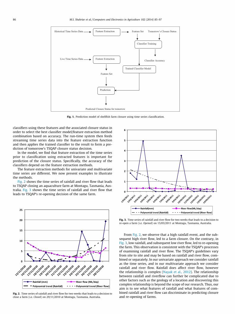
Fig. 1. Prediction model of shellfish farm closure using time series classification.

86 M.S. Shahriar et al. / Computers and Electronics in Agriculture 102 (2014) 85–97

classifiers using these features and the associated closure status inorder to select the best classifier model/feature extraction methodcombination based on accuracy. The run-time system then feedsstreaming time series data into the feature extraction functionand then applies the trained classifier to the result to form a pre-diction of tomorrow’s TSQAP closure status decision.

In the model, we find that feature extraction of the time seriesprior to classification using extracted features is important forprediction of the closure status. Specifically, the accuracy of theclassifiers depend on the feature extraction methods.

The feature extraction methods for univariate and multivariatetime series are different. We now present examples to illustratethe methods.

Fig. 2 shows the time series of rainfall and river flow that leadsto TSQAP closing an aquaculture farm at Montagu, Tasmania, Aus-tralia. Fig. 3 shows the time series of rainfall and river flow thatleads to TSQAP’s re-opening decision of the same farm.

Fig. 2. Time series of rainfall and river flow for two weeks that leads to a decision toclose a farm (i.e. Closed) on 29/11/2010 at Montagu, Tasmania, Australia.

Fig. 3. Time series of rainfall and river flow for two weeks that leads to a decision tore-open a farm (i.e. Opened) on 15/03/2011 at Montagu, Tasmania, Australia.

From Fig. 2, we observe that a high rainfall event, and the sub-sequent high river flow, led to a farm closure. On the contrary, inFig. 3, low rainfall, and subsequent low river flow, led to re-openingthe farm. This observation is consistent with the TSQAP’s processesof examining rainfall and river flow. The TSQAP’s guidelines varyfrom site to site and may be based on rainfall and river flow, com-bined or separately. In our univariate approach we consider rainfallas the time series, and in our multivariate approach we considerrainfall and river flow. Rainfall does affect river flow, howeverthe relationship is complex (Nayak et al., 2012). The relationshipbetween rainfall and riverflow can further be complicated due toother factors such as the geology of a location and discovering thiscomplex relationship is beyond the scope of our research. Thus, ouraim is to see what features of rainfall and what features of com-bined rainfall and river flow can discriminate in predicting closureand re-opening of farms.

−6 −4 −2 0 2 4 6

−0.4

−0.2

0.0

0.2

0.4

Lag

AC

F

Rainfall & Riverflow

−6 −4 −2 0 2 4 6

−0.4

−0.2

0.0

0.2

0.4

0.6

Lag

AC

F

Rainfall & Riverflow

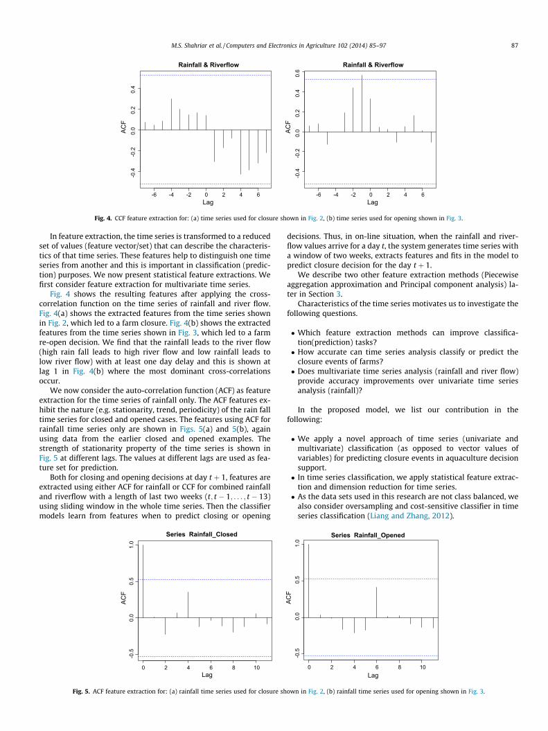
Fig. 4. CCF feature extraction for: (a) time series used for closure shown in Fig. 2, (b) time series used for opening shown in Fig. 3.

M.S. Shahriar et al. / Computers and Electronics in Agriculture 102 (2014) 85–97 87

In feature extraction, the time series is transformed to a reducedset of values (feature vector/set) that can describe the characteris-tics of that time series. These features help to distinguish one timeseries from another and this is important in classification (predic-tion) purposes. We now present statistical feature extractions. Wefirst consider feature extraction for multivariate time series.

Fig. 4 shows the resulting features after applying the cross-correlation function on the time series of rainfall and river flow.Fig. 4(a) shows the extracted features from the time series shownin Fig. 2, which led to a farm closure. Fig. 4(b) shows the extractedfeatures from the time series shown in Fig. 3, which led to a farmre-open decision. We find that the rainfall leads to the river flow(high rain fall leads to high river flow and low rainfall leads tolow river flow) with at least one day delay and this is shown atlag 1 in Fig. 4(b) where the most dominant cross-correlationsoccur.

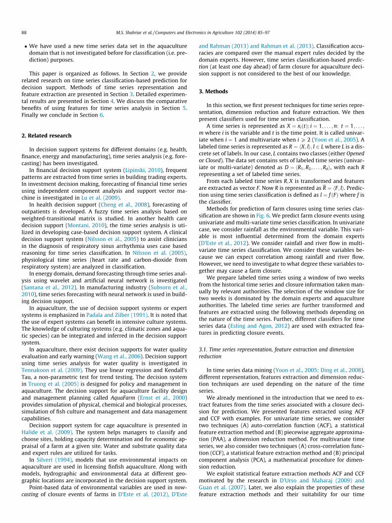
We now consider the auto-correlation function (ACF) as featureextraction for the time series of rainfall only. The ACF features ex-hibit the nature (e.g. stationarity, trend, periodicity) of the rain falltime series for closed and opened cases. The features using ACF forrainfall time series only are shown in Figs. 5(a) and 5(b), againusing data from the earlier closed and opened examples. Thestrength of stationarity property of the time series is shown inFig. 5 at different lags. The values at different lags are used as fea-ture set for prediction.

Both for closing and opening decisions at day t þ 1, features areextracted using either ACF for rainfall or CCF for combined rainfalland riverflow with a length of last two weeks (t; t � 1; . . . ; t � 13)using sliding window in the whole time series. Then the classifiermodels learn from features when to predict closing or opening

0 2 4 6 8 10

Lag

−0.5

0.0

0.5

1.0

AC

F

Series Rainfall_Closed

Fig. 5. ACF feature extraction for: (a) rainfall time series used for closure sh

decisions. Thus, in on-line situation, when the rainfall and river-flow values arrive for a day t, the system generates time series witha window of two weeks, extracts features and fits in the model topredict closure decision for the day t þ 1.

We describe two other feature extraction methods (Piecewiseaggregation approximation and Principal component analysis) la-ter in Section 3.

Characteristics of the time series motivates us to investigate thefollowing questions.

� Which feature extraction methods can improve classifica-tion(prediction) tasks?� How accurate can time series analysis classify or predict the

closure events of farms?� Does multivariate time series analysis (rainfall and river flow)

provide accuracy improvements over univariate time seriesanalysis (rainfall)?

In the proposed model, we list our contribution in thefollowing:

� We apply a novel approach of time series (univariate andmultivariate) classification (as opposed to vector values ofvariables) for predicting closure events in aquaculture decisionsupport.� In time series classification, we apply statistical feature extrac-

tion and dimension reduction for time series.� As the data sets used in this research are not class balanced, we

also consider oversampling and cost-sensitive classifier in timeseries classification (Liang and Zhang, 2012).

0 2 4 6 8 10

−0.5

0.0

0.5

1.0

Lag

AC

F

Series Rainfall_Opened

own in Fig. 2, (b) rainfall time series used for opening shown in Fig. 3.

88 M.S. Shahriar et al. / Computers and Electronics in Agriculture 102 (2014) 85–97

� We have used a new time series data set in the aquaculturedomain that is not investigated before for classification (i.e. pre-diction) purposes.

This paper is organized as follows. In Section 2, we providerelated research on time series classification-based prediction fordecision support. Methods of time series representation andfeature extraction are presented in Section 3. Detailed experimen-tal results are presented in Section 4. We discuss the comparativebenefits of using features for time series analysis in Section 5.Finally we conclude in Section 6.

2. Related research

In decision support systems for different domains (e.g. health,finance, energy and manufacturing), time series analysis (e.g. fore-casting) has been investigated.

In financial decision support system (Lipinski, 2010), frequentpatterns are extracted from time series in building trading experts.In investment decision making, forecasting of financial time seriesusing independent component analysis and support vector ma-chine is investigated in Lu et al. (2009).

In health decision support (Cheng et al., 2008), forecasting ofoutpatients is developed. A fuzzy time series analysis based onweighted-transitional matrix is studied. In another health caredecision support (Montani, 2010), the time series analysis is uti-lized in developing case-based decision support system. A clinicaldecision support system (Nilsson et al., 2005) to assist cliniciansin the diagnosis of respiratory sinus arrhythmia uses case basedreasoning for time series classification. In Nilsson et al. (2005),physiological time series (heart rate and carbon-dioxide fromrespiratory system) are analyzed in classification.

In energy domain, demand forecasting through time series anal-ysis using wavelet and artificial neural network is investigated(Santana et al., 2012). In manufacturing industry (Subsorn et al.,2010), time series forecasting with neural network is used in build-ing decision support.

In aquaculture, the use of decision support systems or expertsystems is emphasized in Padala and Zilber (1991). It is noted thatthe use of expert systems can benefit in intensive culture systems.The knowledge of culturing systems (e.g. climatic zones and aqua-tic species) can be integrated and inferred in the decision supportsystem.

In aquaculture, there exist decision supports for water qualityevaluation and early warning (Wang et al., 2006). Decision supportusing time series analysis for water quality is investigated inTennakoon et al. (2009). They use linear regression and Kendall’sTau, a non-parametric test for trend testing. The decision systemin Truong et al. (2005) is designed for policy and management inaquaculture. The decision support for aquaculture facility designand management planning called AquaFarm (Ernst et al., 2000)provides simulation of physical, chemical and biological processes,simulation of fish culture and management and data managementcapabilities.

Decision support system for cage aquaculture is presented inHalide et al. (2009). The system helps managers to classify andchoose sites, holding capacity determination and for economic ap-praisal of a farm at a given site. Water and substrate quality dataand expert rules are utilized for tasks.

In Silvert (1994), models that use environmental impacts onaquaculture are used in licensing finfish aquaculture. Along withmodels, hydrographic and environmental data at different geo-graphic locations are incorporated in the decision support system.

Point-based data of environmental variables are used in now-casting of closure events of farms in D’Este et al. (2012), D’Este

and Rahman (2013) and Rahman et al. (2013). Classification accu-racies are compared over the manual expert rules decided by thedomain experts. However, time series classification-based predic-tion (at least one day ahead) of farm closure for aquaculture deci-sion support is not considered to the best of our knowledge.

3. Methods

In this section, we first present techniques for time series repre-sentation, dimension reduction and feature extraction. We thenpresent classifiers used for time series classification.

A time series is represented as X ¼ xiðtÞ; i ¼ 1; . . . ;n; t ¼ 1; . . . ;

m where i is the variable and t is the time point. It is called univar-iate when i ¼ 1 and multivariate when i P 2 (Yoon et al., 2005). Alabeled time series is represented as R ¼ hX; li; l 2 L where L is a dis-crete set of labels. In our case, L contains two classes (either Openedor Closed). The data set contains sets of labeled time series (univar-iate or multi-variate) denoted as D ¼ hR1;R2; . . . ;Rdi, with each Rrepresenting a set of labeled time series.

From each labeled time series R;X is transformed and featuresare extracted as vector F. Now R is represented as R ¼ hF; li. Predic-tion using time series classification is defined as l ¼ f ðFÞ where f isthe classifier.

Methods for prediction of farm closures using time series clas-sification are shown in Fig. 6. We predict farm closure events usingunivariate and multi-variate time series classification. In univariatecase, we consider rainfall as the environmental variable. This vari-able is most influential determined from the domain experts(D’Este et al., 2012). We consider rainfall and river flow in multi-variate time series classification. We consider these variables be-cause we can expect correlation among rainfall and river flow.However, we need to investigate to what degree these variables to-gether may cause a farm closure.

We prepare labeled time series using a window of two weeksfrom the historical time series and closure information taken man-ually by relevant authorities. The selection of the window size fortwo weeks is dominated by the domain experts and aquacultureauthorities. The labeled time series are further transformed andfeatures are extracted using the following methods depending onthe nature of the time series. Further, different classifiers for timeseries data (Esling and Agon, 2012) are used with extracted fea-tures in predicting closure events.

3.1. Time series representation, feature extraction and dimensionreduction

In time series data mining (Yoon et al., 2005; Ding et al., 2008),different representation, features extraction and dimension reduc-tion techniques are used depending on the nature of the timeseries.

We already mentioned in the introduction that we need to ex-tract features from the time series associated with a closure deci-sion for prediction. We presented features extracted using ACFand CCF with examples. For univariate time series, we considertwo techniques (A) auto-correlation function (ACF), a statisticalfeature extraction method and (B) piecewise aggregate approxima-tion (PAA), a dimension reduction method. For multivariate timeseries, we also consider two techniques (A) cross-correlation func-tion (CCF), a statistical feature extraction method and (B) principalcomponent analysis (PCA), a mathematical procedure for dimen-sion reduction.

We exploit statistical feature extraction methods ACF and CCFmotivated by the research in D’Urso and Maharaj (2009) andGuan et al. (2007). Later, we also explain the properties of thesefeature extraction methods and their suitability for our time

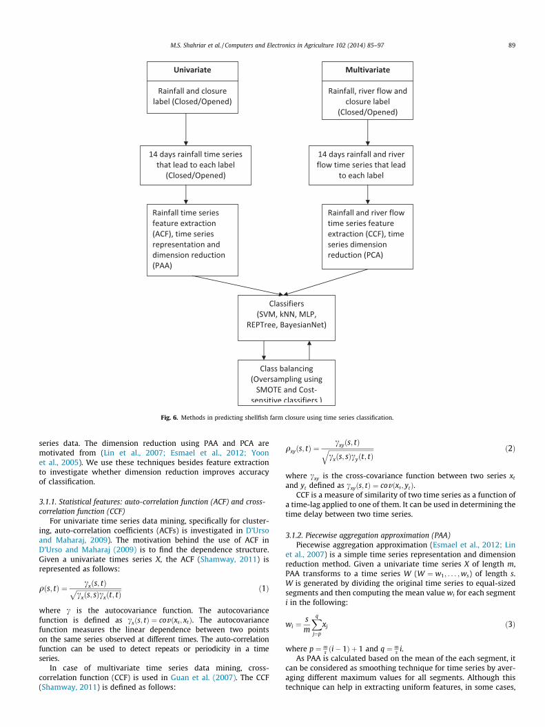
Fig. 6. Methods in predicting shellfish farm closure using time series classification.

M.S. Shahriar et al. / Computers and Electronics in Agriculture 102 (2014) 85–97 89

series data. The dimension reduction using PAA and PCA aremotivated from (Lin et al., 2007; Esmael et al., 2012; Yoonet al., 2005). We use these techniques besides feature extractionto investigate whether dimension reduction improves accuracyof classification.

3.1.1. Statistical features: auto-correlation function (ACF) and cross-correlation function (CCF)

For univariate time series data mining, specifically for cluster-ing, auto-correlation coefficients (ACFs) is investigated in D’Ursoand Maharaj, 2009). The motivation behind the use of ACF inD’Urso and Maharaj (2009) is to find the dependence structure.Given a univariate times series X, the ACF (Shamway, 2011) isrepresented as follows:

qðs; tÞ ¼ cxðs; tÞffiffiffiffiffiffiffiffiffiffiffiffiffiffiffiffiffiffiffiffiffiffiffiffiffiffiffifficxðs; sÞcxðt; tÞ

p ð1Þ

where c is the autocovariance function. The autocovariancefunction is defined as cxðs; tÞ ¼ covðxs; xtÞ. The autocovariancefunction measures the linear dependence between two pointson the same series observed at different times. The auto-correlationfunction can be used to detect repeats or periodicity in a timeseries.

In case of multivariate time series data mining, cross-correlation function (CCF) is used in Guan et al. (2007). The CCF(Shamway, 2011) is defined as follows:

qxyðs; tÞ ¼cxyðs; tÞffiffiffiffiffiffiffiffiffiffiffiffiffiffiffiffiffiffiffiffiffiffiffiffiffiffiffiffi

cxðs; sÞcyðt; tÞq ð2Þ

where cxy is the cross-covariance function between two series xt

and yt defined as cxyðs; tÞ ¼ covðxs; ytÞ.CCF is a measure of similarity of two time series as a function of

a time-lag applied to one of them. It can be used in determining thetime delay between two time series.

3.1.2. Piecewise aggregation approximation (PAA)Piecewise aggregation approximation (Esmael et al., 2012; Lin

et al., 2007) is a simple time series representation and dimensionreduction method. Given a univariate time series X of length m,PAA transforms to a time series W (W ¼ w1; . . . ;ws) of length s.W is generated by dividing the original time series to equal-sizedsegments and then computing the mean value wi for each segmenti in the following:

wi ¼sm

Xq

j¼p

xj ð3Þ

where p ¼ ms ði� 1Þ þ 1 and q ¼ m

s i.As PAA is calculated based on the mean of the each segment, it

can be considered as smoothing technique for time series by aver-aging different maximum values for all segments. Although thistechnique can help in extracting uniform features, in some cases,

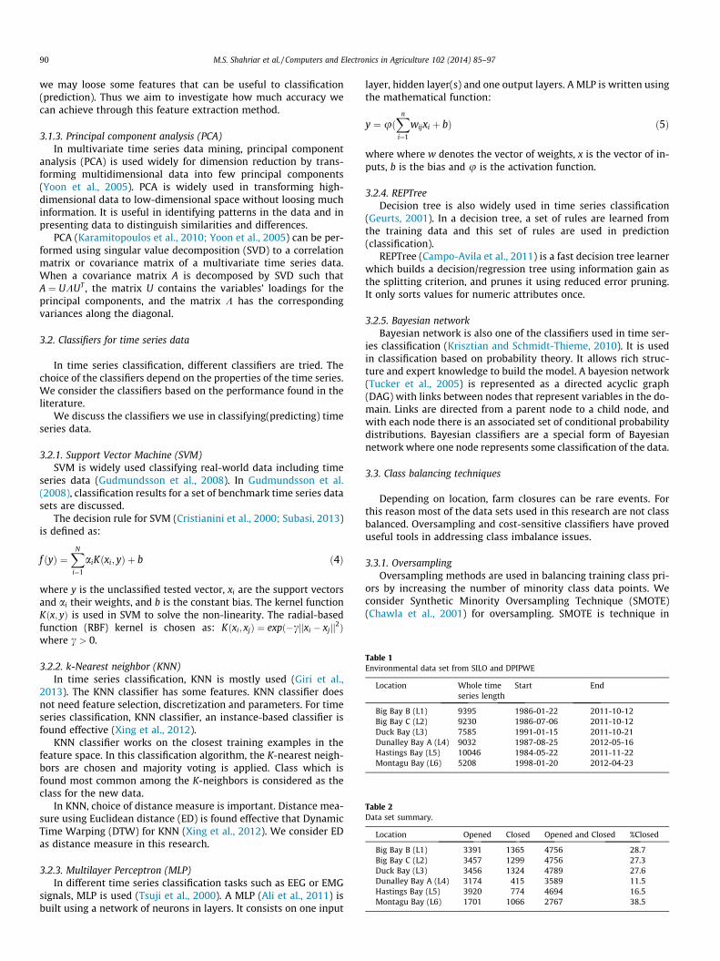
Table 1Environmental data set from SILO and DPIPWE

Location Whole timeseries length

Start End

Big Bay B (L1) 9395 1986-01-22 2011-10-12Big Bay C (L2) 9230 1986-07-06 2011-10-12Duck Bay (L3) 7585 1991-01-15 2011-10-21Dunalley Bay A (L4) 9032 1987-08-25 2012-05-16Hastings Bay (L5) 10046 1984-05-22 2011-11-22Montagu Bay (L6) 5208 1998-01-20 2012-04-23

Table 2Data set summary.

Location Opened Closed Opened and Closed %Closed

Big Bay B (L1) 3391 1365 4756 28.7Big Bay C (L2) 3457 1299 4756 27.3Duck Bay (L3) 3456 1324 4789 27.6Dunalley Bay A (L4) 3174 415 3589 11.5Hastings Bay (L5) 3920 774 4694 16.5Montagu Bay (L6) 1701 1066 2767 38.5

90 M.S. Shahriar et al. / Computers and Electronics in Agriculture 102 (2014) 85–97

we may loose some features that can be useful to classification(prediction). Thus we aim to investigate how much accuracy wecan achieve through this feature extraction method.

3.1.3. Principal component analysis (PCA)In multivariate time series data mining, principal component

analysis (PCA) is used widely for dimension reduction by trans-forming multidimensional data into few principal components(Yoon et al., 2005). PCA is widely used in transforming high-dimensional data to low-dimensional space without loosing muchinformation. It is useful in identifying patterns in the data and inpresenting data to distinguish similarities and differences.

PCA (Karamitopoulos et al., 2010; Yoon et al., 2005) can be per-formed using singular value decomposition (SVD) to a correlationmatrix or covariance matrix of a multivariate time series data.When a covariance matrix A is decomposed by SVD such thatA ¼ UKUT , the matrix U contains the variables’ loadings for theprincipal components, and the matrix K has the correspondingvariances along the diagonal.

3.2. Classifiers for time series data

In time series classification, different classifiers are tried. Thechoice of the classifiers depend on the properties of the time series.We consider the classifiers based on the performance found in theliterature.

We discuss the classifiers we use in classifying(predicting) timeseries data.

3.2.1. Support Vector Machine (SVM)SVM is widely used classifying real-world data including time

series data (Gudmundsson et al., 2008). In Gudmundsson et al.(2008), classification results for a set of benchmark time series datasets are discussed.

The decision rule for SVM (Cristianini et al., 2000; Subasi, 2013)is defined as:

f ðyÞ ¼XN

i¼1

aiKðxi; yÞ þ b ð4Þ

where y is the unclassified tested vector, xi are the support vectorsand ai their weights, and b is the constant bias. The kernel functionKðx; yÞ is used in SVM to solve the non-linearity. The radial-basedfunction (RBF) kernel is chosen as: Kðxi; xjÞ ¼ expð�cjjxi � xjjj2Þwhere c > 0.

3.2.2. k-Nearest neighbor (KNN)In time series classification, KNN is mostly used (Giri et al.,

2013). The KNN classifier has some features. KNN classifier doesnot need feature selection, discretization and parameters. For timeseries classification, KNN classifier, an instance-based classifier isfound effective (Xing et al., 2012).

KNN classifier works on the closest training examples in thefeature space. In this classification algorithm, the K-nearest neigh-bors are chosen and majority voting is applied. Class which isfound most common among the K-neighbors is considered as theclass for the new data.

In KNN, choice of distance measure is important. Distance mea-sure using Euclidean distance (ED) is found effective that DynamicTime Warping (DTW) for KNN (Xing et al., 2012). We consider EDas distance measure in this research.

3.2.3. Multilayer Perceptron (MLP)In different time series classification tasks such as EEG or EMG

signals, MLP is used (Tsuji et al., 2000). A MLP (Ali et al., 2011) isbuilt using a network of neurons in layers. It consists on one input

layer, hidden layer(s) and one output layers. A MLP is written usingthe mathematical function:

y ¼ uðXn

i¼1

wijxi þ bÞ ð5Þ

where where w denotes the vector of weights, x is the vector of in-puts, b is the bias and u is the activation function.

3.2.4. REPTreeDecision tree is also widely used in time series classification

(Geurts, 2001). In a decision tree, a set of rules are learned fromthe training data and this set of rules are used in prediction(classification).

REPTree (Campo-Avila et al., 2011) is a fast decision tree learnerwhich builds a decision/regression tree using information gain asthe splitting criterion, and prunes it using reduced error pruning.It only sorts values for numeric attributes once.

3.2.5. Bayesian networkBayesian network is also one of the classifiers used in time ser-

ies classification (Krisztian and Schmidt-Thieme, 2010). It is usedin classification based on probability theory. It allows rich struc-ture and expert knowledge to build the model. A bayesion network(Tucker et al., 2005) is represented as a directed acyclic graph(DAG) with links between nodes that represent variables in the do-main. Links are directed from a parent node to a child node, andwith each node there is an associated set of conditional probabilitydistributions. Bayesian classifiers are a special form of Bayesiannetwork where one node represents some classification of the data.

3.3. Class balancing techniques

Depending on location, farm closures can be rare events. Forthis reason most of the data sets used in this research are not classbalanced. Oversampling and cost-sensitive classifiers have proveduseful tools in addressing class imbalance issues.

3.3.1. OversamplingOversampling methods are used in balancing training class pri-

ors by increasing the number of minority class data points. Weconsider Synthetic Minority Oversampling Technique (SMOTE)(Chawla et al., 2001) for oversampling. SMOTE is technique in

M.S. Shahriar et al. / Computers and Electronics in Agriculture 102 (2014) 85–97 91

which the minority class is over-sampled by creating syntheticexamples rather than by over-sampling with replacement. The ideabehind this method is to artificially generate new sample of minor-ity class using the nearest neighbors of these cases.

3.3.2. Cost-sensitive classifierCost-sensitive classification is a technique that takes the

misclassification costs (and possibly other types of cost) into con-sideration (Ling and Sheng, 2008). The goal of this type of learning

Table 3Parameters for classifiers.

Support VectorMachine (SVM)

K-Nearest Neighborhood(K-NN)

Multi Layer Perceptron(MLP)

Cost = 1.0 K = 1 Hidden layer = 1Gamma = 0.0 Distance

measure = EuclideanLearning rate=0.3

Kernel = RBF Momentum = 0.2Epochs = 500Activationfunction = Sigmoid

Table 4Parameters for SMOTE.

Location/data set Perc. over

Big Bay B (L1) 300Big Bay C (L2) 300Duck Bay (L3) 300Dunalley Bay A (L4) 600Hastings Bay (L5) 400

Table 5Parameters for cost-sensitive classifiers.

Location/data set (Closed,Opened)

Big Bay B (L1) (3,1)Big Bay C (L2) (3,1)Duck Bay (L3) (3,1)Dunalley Bay A (L4) (6,1)Hastings Bay (L5) (5,1)

Table 6Rainfall time series as feature.

L SVM 1NN MLP

Ov. Op. Cl. Ov. Op. Cl. Ov.

L1 71.2 99.9 0 68.2 79.9 39.3 74.9L2 72.7 99.9 0 68.3 80.7 35.2 73.2L3 72.4 99.9 0 69.4 81.1 38.7 76.1L4 88.4 99.9 0 82.2 89.9 23.1 89.0L5 83.5 100.0 0 79.1 90.2 23.3 85.5L6 69.3 63.6 78.6 62.1 72.3 45.9 71.3

Table 7Extracted PAA features from rainfall time series.

L SVM 1NN MLP

Ov. Op. Cl. Ov. Op. Cl. Ov.

L1 93.0 100 75.7 66.7 80.0 33.8 71.3L2 93.9 100 77.7 66.7 80.2 31.0 72.7L3 92.6 100 73.3 66.1 81.2 34.0 72.3L4 94.0 99.9 48.4 80.6 88.8 18.2 88.2L5 95.4 100 72.9 77.3 88.2 21.8 83.3L6 98.4 99.7 96.3 58.0 67.9 42.2 61.3

is to minimize the total cost. We consider the cost-sensitive classi-fier using reweighted training instances.

4. Experimental results

In this section, we present experimental results. First, wediscuss the data set and parameters for classifiers used in experi-ments. We then present the results of univariate and multi-variatetime series classification. In each case, we present results of classi-fication using time series data as feature and using transformed(extracted) features of time series data. For all experiments, weuse R programming language (R2013) for feature extraction andRWeka package (RWeka, 2013) for accessing classifiers in WEKA(Hall et al., 2009) data mining and machine learning toolbox.

4.1. Data set description

In this research, we consider daily rainfall for six locations(L1–L6) and river flow for three locations (L3, L4, L6) in Tasmania,Australia shown in Table 1. Data are collected from SILO (Govern-ment et al., 2012) and the Department of Primary Industries, Parks,Water and Environment (DPIPWE). Aquaculture farm closure infor-mation (i.e. labels) are collected from Tasmanian Shellfish QualityAssurance Program (TSQAP), Department of Health and HumanServices.

4.2. Data preprocessing

For each closure class, we associate rainfall for last two weeks inunivariate time series classification. For multivariate time seriesclassification, we associate rainfall and river flow for the last twoweeks for each class.

As there are no corresponding closure information available forsome days in Table 1, we omit those samples of environmentalvariables (rainfall and river flow) from whole time series whenwe label the time series of two weeks that lead to a decision(Closed/Opened).

In Table 2, we present the number of opening (i.e. Opened class)and closure (i.e. Closed class) and percentage of the closure of thefarms. We observe that data for all locations are class imbalancedexcept Montagu Bay (L6).

REPTree BayesianNet

Op. Cl. Ov. Op. Cl. Ov. Op. Cl.

86.6 45.9 73.9 86.8 41.9 76.1 77.5 72.596.0 12.7 73.9 89.7 31.9 75.0 76.6 70.888.5 43.5 74.5 87.6 40.2 77.4 78.8 73.899.1 12.3 88.4 99.2 5.8 88.3 98.8 8.294.5 39.5 82.8 96.6 12.5 83.1 91.0 43.272.4 69.7 66.4 78.5 46.9 71.0 75.0 64.7

REPTree BayesianNet

Op. Cl. Ov. Op. Cl. Ov. Op. Cl.

100 0 70.2 88.4 25.1 68.9 79.1 43.7100 0 71.4 90.8 19.9 69.9 81.4 39.5100 0 71.3 87.3 29.4 69.7 78.6 46.4100 0 88.0 99.5 1.5 88.2 100 099.6 1.2 83.0 98.5 4.7 82.1 95.3 15.699.6 0.5 61.4 77.5 35.8 61.8 68.7 50.8

Table 8Extracted ACF features from rainfall time series.

L SVM 1NN MLP REPTree BayesianNet

Ov. Op. Cl. Ov. Op. Cl. Ov. Op. Cl. Ov. Op. Cl. Ov. Op. Cl.

L1 93.3 100 76.8 80.9 87.7 64.2 70.9 96.3 8.0 71.7 88.3 30.6 68.6 81.6 36.4L2 94.2 100 78.7 85.5 88.2 63.4 72.3 97.7 4.9 71.7 87.7 29.0 68.6 81.5 34.3L3 93.0 99.9 74.8 80.8 88.0 66.0 72.2 97.3 6.8 72.7 88.5 31.3 69.6 81.2 39.4L4 92.4 99.9 52.5 88.4 93.9 46.9 88.2 100 0 88.0 97.6 15.7 88.2 100 0L5 95.7 100 74.0 86.0 92.3 54.1 83.5 99.3 3.2 82.2 96.6 9.0 82.2 96.7 8.9L6 98.6 99.7 96.7 80.8 84.7 74.5 62.4 85.4 25.9 68.7 78.9 52.5 62.7 73.6 45.3

Fig. 7. Accuracy with SVM using PAA and ACF features for the Closed class only.

(a)

(b)

(c)Fig. 8. Accuracy for SVM using no class balancing, SMOTE (oversampling) and cost-sensitive classifier for PAA. (a) Overall (b) Opened class (c) Closed class.

92 M.S. Shahriar et al. / Computers and Electronics in Agriculture 102 (2014) 85–97

4.3. Parameters for classifiers

In Table 3, parameters of SVM, K-NN and MLP are presented. Weuse LibSVM in WEKA for SVM with cost 1.0, Gamma 0.0 and RBFKernel. We use 1-nearest neighborhood (1-NN) because most re-search on time series classification performs best with 1-NN (Xinget al., 2012). In MLP, we use 1 hidden layer.

We consider 10-fold cross validation for experiments. By 10-fold cross validation, it means that the data is split into 10 groupswhere nine groups are considered for training and the remainingone group is considered for testing. This process is repeated forall 10 groups.

4.4. parameters for class balancing

In Table 4, we present the parameters for oversampling usingSMOTE function in R DMwR package (DMwR, 2013). For example,perc.over with value 300 means that 3 examples will be createdfor each case in the initial dataset that belongs to the minorityclass.

The cost parameters used in cost-sensitive classifiers arepresented in Table 5. The cost parameters are calculated basedon the ratio of samples of two classes (Opened and Closed). Forexample, if the total samples are 800 (Closed = 200 andOpened = 600), then the cost parameter is (3,1).

4.5. Classification accuracy

Classification (prediction) accuracy is considered for Overall(forOpened and Closed class together), and Opened class and Closedclass separately. The accuracy of the Closed class is the most signif-icant in decision making by the relevant authorities due to the im-pact of consuming contaminated shellfish for human health. The

closure reasons are based on mainly health issues impacted frommicrobial (e.g. coliform). It is confirmed from the relevant author-ities and our analysis that rainfall and hence river flow are the ma-jor contributing factors to coliform that affects human health.Thus, the classification accuracy of the Closed class is an importantfeature for the decision support.

The classification accuracy presented in this research is theindication of the capability of the decision support to predict theclosure or opening the shellfish farms one day ahead. In other

M.S. Shahriar et al. / Computers and Electronics in Agriculture 102 (2014) 85–97 93

words, it shows how correctly we can predict closing and openingdecision. Currently, the authorities or managers use daily manualdecisions of closing and opening based on the observations andtheir knowledge. Our aim is to aid in making their decisions andcurrently this is also a requirement from them.

It is worth mentioning that the likelihood of closure (eitheropened or closed) can be measured using the time series andclassifiers. The likelihood of the closure (we call distance measure)can be for multiple days ahead prediction as well. However, at thismoment, this is a future requirement by the relevant authorities inthe decision support.

We denote Ov. for Overall, Op. for Opened class and Cl. for Closedclass to represent accuracy in %.

4.6. Univariate time series classification

We first present the results using time series of rainfall data. Wethen present results using PAA and ACF features of rainfall time

(a)

(b)

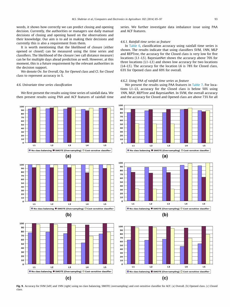
(c)Fig. 9. Accuracy for SVM (left) and 1NN (right) using no class balancing, SMOTE (oversamclass.

series. We further investigate data imbalance issue using PAAand ACF features.

4.6.1. Rainfall time series as featureIn Table 6, classification accuracy using rainfall time series is

shown. The results indicate that using classifiers SVM, 1NN, MLPand REPTree, the accuracy for the Closed class is very low for fivelocations (L1–L5). BayesianNet shows the accuracy above 70% forthree locations (L1–L3) and shows low accuracy for two locations(L4–L5). The accuracy for the location L6 is 78% for Closed class,63% for Opened class and 69% for overall.

4.6.2. Using PAA of rainfall time series as featureWe present the results using PAA features in Table 7. For loca-

tions L1–L5, accuracy for the Closed class is below 50% using1NN, MLP, REPTree and BayesianNet. In SVM, the overall accuracyand the accuracy for Closed and Opened class are above 73% for all

(a)

(b)

(c)pling) and cost-sensitive classifier for ACF. (a) Overall. (b) Opened class. (c) Closed

94 M.S. Shahriar et al. / Computers and Electronics in Agriculture 102 (2014) 85–97

locations except L4. For the location L6, the accuracy using SVM is96% for Closed class, 99% for Opened class and 98% overall. Weobserve that PAA feature extraction improves accuracy over therainfall time series using SVM classifier.

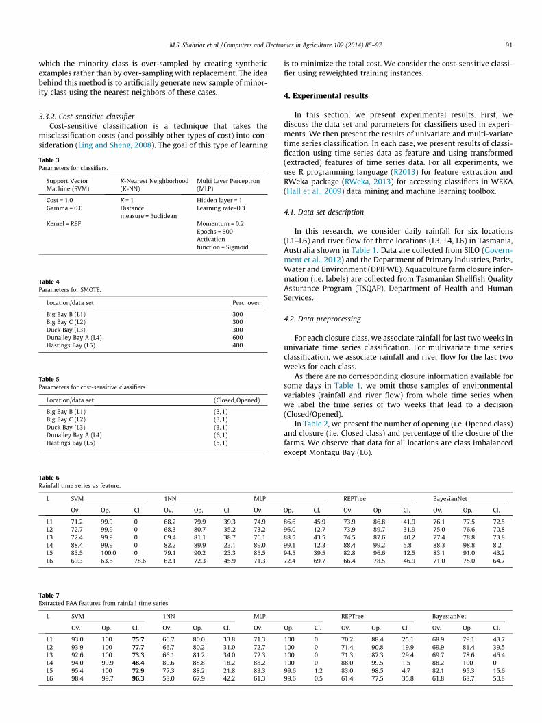
4.6.3. Using ACF of rainfall time series as featureWe present results using ACF features in Table 8. SVM has

the accuracy above 74% for locations except L4. For locationL6, SVM shows the accuracy over 96% for Closed and Openedclasses.

Unlike using PAA, 1NN shows reasonable accuracy using ACF. Itshows accuracy over 63% for Closed class for locations L1, L2, L3and L6. However, for all locations, accuracy of the Closed class isbelow 53% using MLP, REPTree and BayesianNet. We observe thatACF features improves the accuracy over the rainfall time seriesfeature using SVM and 1-NN classifiers.

In Fig. 7, we show the comparison of accuracy of the Closedclass using PAA and ACF features with SVM. We observe that ACFis performing over PAA for all locations. Although, the accuracyfor the location L4 is below 60%(possibly due to unbalance data,see Table 2), accuracy for other locations is above 70% that is help-ful for the relevant authorities in decision making.

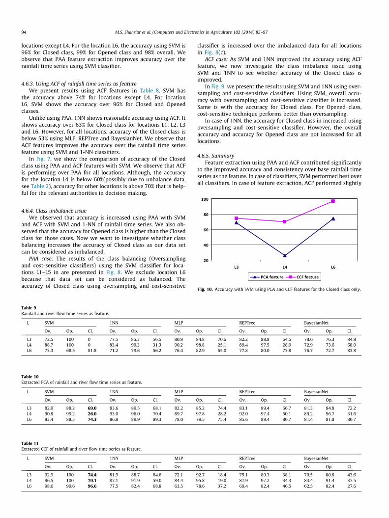
Fig. 10. Accuracy with SVM using PCA and CCF features for the Closed class only.

4.6.4. Class imbalance issueWe observed that accuracy is increased using PAA with SVM

and ACF with SVM and 1-NN of rainfall time series. We also ob-served that the accuracy for Opened class is higher than the Closedclass for those cases. Now we want to investigate whether classbalancing increases the accuracy of Closed class as our data setcan be considered as imbalanced.

PAA case: The results of the class balancing (Oversamplingand cost-sensitive classifiers) using the SVM classifier for loca-tions L1–L5 in are presented in Fig. 8. We exclude location L6because that data set can be considered as balanced. Theaccuracy of Closed class using oversampling and cost-sensitive

Table 9Rainfall and river flow time series as feature.

L SVM 1NN MLP

Ov. Op. Cl. Ov. Op. Cl. Ov.

L3 72.5 100 0 77.5 85.3 56.5 80.9L4 88.7 100 0 83.4 90.3 31.3 90.2L6 73.3 68.5 81.8 71.2 79.6 56.2 76.4

Table 10Extracted PCA of rainfall and river flow time series as feature.

L SVM 1NN MLP

Ov. Op. Cl. Ov. Op. Cl. Ov.

L3 82.9 88.2 69.0 83.6 89.5 68.1 82.2L4 90.8 99.2 26.0 93.0 96.0 70.4 89.7L6 83.4 88.5 74.3 86.8 89.9 89.3 78.0

Table 11Extracted CCF of rainfall and river flow time series as feature.

L SVM 1NN MLP

Ov. Op. Cl. Ov. Op. Cl. Ov.

L3 92.9 100 74.4 81.9 88.7 64.6 72.1L4 96.5 100 70.1 87.1 91.9 59.0 84.4L6 98.6 99.6 96.6 77.5 82.4 68.8 63.5

classifier is increased over the imbalanced data for all locationsin Fig. 8(c).

ACF case: As SVM and 1NN improved the accuracy using ACFfeature, we now investigate the class imbalance issue usingSVM and 1NN to see whether accuracy of the Closed class isimproved.

In Fig. 9, we present the results using SVM and 1NN using over-sampling and cost-sensitive classifiers. Using SVM, overall accu-racy with oversampling and cost-sensitive classifier is increased.Same is with the accuracy for Closed class. For Opened class,cost-sensitive technique performs better than oversampling.

In case of 1NN, the accuracy for Closed class in increased usingoversampling and cost-sensitive classifier. However, the overallaccuracy and accuracy for Opened class are not increased for alllocations.

4.6.5. SummaryFeature extraction using PAA and ACF contributed significantly

to the improved accuracy and consistency over base rainfall timeseries as the feature. In case of classifiers, SVM performed best overall classifiers. In case of feature extraction, ACF performed slightly

REPTree BayesianNet

Op. Cl. Ov. Op. Cl. Ov. Op. Cl.

84.8 70.6 82.2 88.8 64.5 78.6 76.3 84.898.8 25.1 89.4 97.5 28.0 72.9 73.6 68.082.9 65.0 77.8 80.0 73.8 76.7 72.7 83.8

REPTree BayesianNet

Op. Cl. Ov. Op. Cl. Ov. Op. Cl.

85.2 74.4 83.1 89.4 66.7 81.3 84.8 72.297.8 28.2 92.0 97.4 50.1 89.2 96.7 31.679.5 75.4 85.6 88.4 80.7 81.4 81.8 80.7

REPTree BayesianNet

Op. Cl. Ov. Op. Cl. Ov. Op. Cl.

92.7 18.4 75.1 89.3 38.1 70.5 80.8 43.695.8 19.0 87.9 97.2 34.3 83.4 91.4 37.578.6 37.2 69.4 82.4 46.5 62.5 82.4 27.6

(a)

(b)

(c)

(a)

(b)

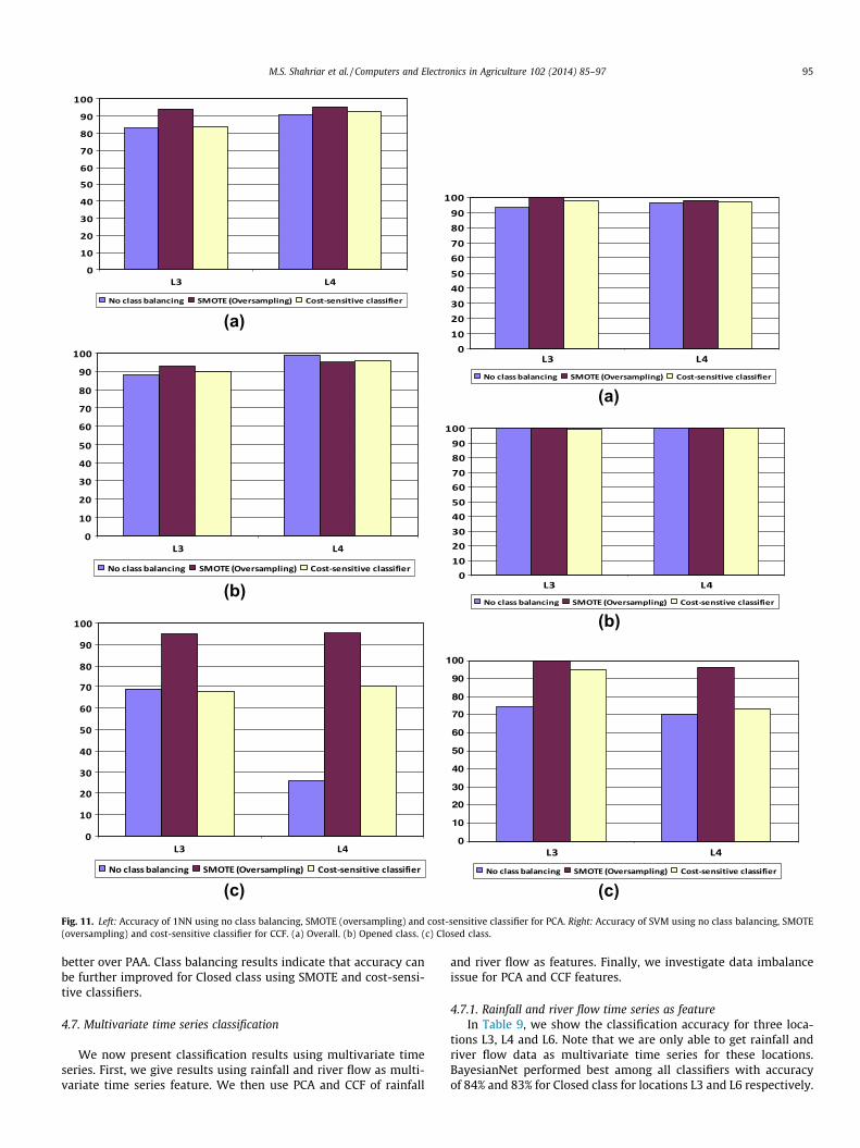
(c)Fig. 11. Left: Accuracy of 1NN using no class balancing, SMOTE (oversampling) and cost-sensitive classifier for PCA. Right: Accuracy of SVM using no class balancing, SMOTE(oversampling) and cost-sensitive classifier for CCF. (a) Overall. (b) Opened class. (c) Closed class.

M.S. Shahriar et al. / Computers and Electronics in Agriculture 102 (2014) 85–97 95

better over PAA. Class balancing results indicate that accuracy canbe further improved for Closed class using SMOTE and cost-sensi-tive classifiers.

4.7. Multivariate time series classification

We now present classification results using multivariate timeseries. First, we give results using rainfall and river flow as multi-variate time series feature. We then use PCA and CCF of rainfall

and river flow as features. Finally, we investigate data imbalanceissue for PCA and CCF features.

4.7.1. Rainfall and river flow time series as featureIn Table 9, we show the classification accuracy for three loca-

tions L3, L4 and L6. Note that we are only able to get rainfall andriver flow data as multivariate time series for these locations.BayesianNet performed best among all classifiers with accuracyof 84% and 83% for Closed class for locations L3 and L6 respectively.

96 M.S. Shahriar et al. / Computers and Electronics in Agriculture 102 (2014) 85–97

However, the overall accuracy is maximum 78% for the location L3.Thus we use PCA and CCF for feature extraction methods in thefollowing.

4.7.2. Using PCA for rainfall and river flow time seriesIn Table 10, we show the accuracy of classification using PCA

feature of rainfall and river flow time series. 1NN performed bestamong all classifiers with accuracy of 89% for the Closed classand overall 86% for the location L6. We observe that the accuracyis increased using PCA features of rainfall and river flow timeseries.

4.7.3. Using CCF of rainfall and river flow as featureWe now present the accuracy of classifiers using CCF features of

rainfall and river flow time series. In Table 11, we observe that SVMperformed best among all classifiers with accuracy of 96% for theClosed class for location L6. For locations L3 and L4, we get accu-racy 74% and 70% respectively. We observe that accuracy usingCCF feature is improved over the rainfall and river flow time seriesas features.

We show the comparison of accuracy of the Closed class onlyusing PCA and CCF features with SVM in Fig. 10. We find that theaccuracy using CCF is higher than that of PCA. The accuracy forthe location L4 is the lowest among other locations and the possi-ble reason is the imbalance data (see Table 2).

4.7.4. Class imbalance issueWe now want to investigate whether class balancing improves

the accuracy of prediction of closure events. In Fig. 11 [Left], weshow the accuracy of 1NN using no balancing, oversampling andcost-sensitive classifier for PCA features. We observe that accuracyis increased for oversampling in all cases. In case of cost-sensitiveclassifier, accuracy is increased for some cases.

The accuracy of SVM using CCF features with no balancing,oversampling and cost-sensitive classifier is shown in Fig. 11[Right]. Again, the accuracy is increased for oversampling in allcases.

4.7.5. SummaryBoth CCF and PCA features improve overall accuracy up to 25%

compared to the rainfall and river flow time series as feature. Incase of feature, CCF gives the better accuracy over PCA. SVM per-forms best among all classifiers. Class balancing also improvesthe accuracy of the Closed class using SMOTE.

5. Discussion

We presented results using univariate and multivariate timeseries classification for predicting farm closure events.

In univariate, we considered rainfall time series and in multi-variate time series, we considered rainfall and river flow time ser-ies. We found the statistical features using autocorrelation function(ACF) performed better over the piecewise aggregate approxima-tion (PAA). In PAA, as time series is first normalized and then piece-wise aggregated, the noise or outliers are transformed. This mayresult in loosing the events (high rainfall) as distinguishable fea-tures for the classes.

In multivariate time series of rainfall and river flow, statisticalfeatures using cross-correlation function (CCF) again performedbetter over the principal component analysis (PCA). CCF can cap-ture time lagged coefficient as feature. This property is possibly oc-curred in the data sets because the rainfall affects/causes the riverflow with possible time lags. This property is shown in Fig. 3 as anexample. Thus this time lagged coefficient may not be captured byPCA.

Support vector machine performed best among all classifiers forACF features in univariate and for CCF features in multivariate timeseries. 1-NN is found the next effective classifier with ACF featurefor rainfall time series and PCA features for rainfall and river flowtime series.

Class balancing using SMOTE and using cost-sensitive classifiersfor imbalanced data show improvement of classification accuracy,specifically for Closed class which is important for the shellfishfarm closure decision support system.

6. Conclusions and future work

We studied the novel application of time series classification inpredicting aquaculture farm closures for aquaculture decision sup-port. Statistical features analysis using auto correlation functionand cross correlation function are exploited for univariate andmultivariate time series analysis. Feature extraction by dimensionreduction using piecewise aggregate approximation and principalcomponent analysis are also investigated. Experimental resultsestablish the applicability of auto-correlation function as featureover piecewise aggregate approximation feature with support vec-tor machine for univariate time series. We achieve up to 30% over-all accuracy improvement applying autocorrelation functioncompared to the rainfall time series. In multivariate analysis, fea-ture analysis using cross-correlation function performs better overprincipal component analysis using support vector machine asclassifier. We achieve up to 25% overall accuracy improvementapplying cross-correlation function compared to the rainfall andriver flow time series. Finally, class balancing using SMOTE andcost-sensitive classifiers show that the accuracy of predicting clo-sures can be improved if data is balanced.

In future, we plan to use extend this prediction model havingexplanation capability of causing closures. In this case, we planto study multivariate pattern (rules or motifs) discovery that causeclosure events.

Acknowledgements

The Intelligent Sensing and Systems Laboratory and the Tasma-nian node of the Australian Centre for Broadband Innovation isassisted by a grant from the Tasmanian Government which isadministered by the Tasmanian Department of Economic Develop-ment, Tourism and the Arts. This research is also supported withAquaculture Decision Support (AquaDS) project under CSIRO FoodFutures Flagship.

References

Ali, A., Ghazali, R., Mat Deris, M., 2011. The wavelet multilayer perceptron for theprediction of earthquake time series data. In: Proceedings of the 13thInternational Conference on Information Integration and Web-basedApplications and Services (iiWAS ’11). ACM, New York, NY, USA, pp. 138–143.

Campo-Avila, J., Moreno-Vergara, N., Trella-L’pez, M., 2011. Analizying factors toincrease the influence of a twitter user. Adv. Intell. Soft Comput. 89, 69–76.

Chawla, N.V., Bowyer, K.W., Hall, L.O., Kegelmeyer, W.P., 2001. Synthetic minorityover-sampling technique. J. Artif. Intell. Res. 16, 321–357.

Cheng, C.H., Wang, J.W., Li, C.H., 2008. Forecasting the number of outpatient visitsusing a new fuzzy time series based on weighted-transitional matrix. Exp. Syst.Appl. 34 (4), 2568–2575.

Chi, H.-M., Moskowitza, H., Ersoyb, O.K., Altinkemera, K., Gavinc, P.F., Huffc, B.E.,Olsenc, B.A., 2009. Machine learning and genetic algorithms in pharmaceuticaldevelopment and manufacturing processes. Decis. Supp. Syst. 48 (1), 69–80.

Cristianini, Nello, Shawe-Taylor, John, 2000. An Introduction to Support VectorMachines: And Other Kernel-Based Learning Methods. Cambridge UniversityPress, Cambridge, England.

D’Este, C., Rahman, A., 2013. Similarity weighted ensembles for relocating models ofrare events. MCS, LNCS 7872, 25–36.

D’Este, C., Rahman, A., Turnbull, A., 2012. Predicting shellfish farm closures withclass balancing methods. In: Australian AI Conference, pp. 39–48.

M.S. Shahriar et al. / Computers and Electronics in Agriculture 102 (2014) 85–97 97

Ding, H., Trajcevski, G., Scheuermann, P., Wang, X., Keogh, E., 2008. Querying andmining of time series data: experimental comparison of representations anddistance measures. J. Proc. VLDB Endow. 1 (2), 1542–1552.

<http://cran.r-project.org/web/packages/DMwR/index.html>.D’Urso, P., Maharaj, E.A., 2009. Autocorrelation-based fuzzy clustering of timeseries.

Fuzzy Sets Syst. 160, 3565–3589.Ernst, D.H., Bolte, J.P., Nath, S.S., 2000. AquaFarm: simulation and decision support

for aquaculture facility design and management planning. Aquacult. Eng. 23,121–179.

Esling, P., Agon, C., 2012. Time-series data mining. ACM Comput. Surv. 45(1), Article12.

Esmael, B., Arnaout, A., Fruhwirth, R.K., Thonhauser, G., 2012. Multivariate timeseries classification by combining trend-based and value-basedapproximations. ICCSA 2012, Part IV, LNCS 7336, 392–403.

Geurts, P., 2001. Pattern extraction for time series classification. In: Proceedings ofPrinciples of Data Mining and Knowledge Discovery, 5th European Conference,2001 September 3–5, Freiburg, Germany, pp. 115–127.

Giri, D., Acharaya, R., Martis, R.Y., Sree, S.V., Lim, T.C., Ahmed, T., Suri, J.S., 2013.Automated diagnosis of Coronary Artery Disease affected patients using LDA,PCA, ICA and discrete wavelet transform. Know.-based Syst. 37, 274–282.

Queensland Government, 2012. SILO Climate Data. <http://www.longpaddock.qld.gov.au/silo/> (accessed 10.12).

Guan, H., Jiang, Q., Hong, Z., 2007. A new metric for classification of multivariatetime series. Fuzzy Syst. Know. Discov., FSKD 2007, 453–457.

Gudmundsson, S., Runarsson, T.P., Sigurdsson, S., 2008. Support vector machinesand dynamic time warping for time series. IJCNN 2008, 2772–2776.

Halide, H., Stigebrandt, A., Rehbein, M., McKinnon, A.D., 2009. Developing a decisionsupport system for sustainable cage aquaculture. Environ. Model. Softw. 24 (6),694–702.

Hall, Mark, Frank, Eibe, Holmes, Geoffrey, Pfahringer, Bernhard, Reutemann, Peter,Witten, Ian H., 2009. The WEKA data mining software: an update. SIGKDDExplor. 11(1).

Karamitopoulos, L., Evangelidis, G., Dervos, D., 2010. PCA-based time seriessimilarity search, data mining. Ann. Inf. Syst. 8, 255–276.

Khan, A., Doucette, J.A., Cohen, R., Lizotte, D.J., 2012. Integrating machine learninginto a medical decision support system to address the problem of missingpatient data. In: 11th International Conference on Machine Learning andApplications, pp. 454–457.

Krisztian, B., Schmidt-Thieme, L., 2010. Motif-based classification of time serieswith Bayesian networks and SVMs. Adv. Data Anal. Data Handl. Bus. Intell. Stud.Classif. Data Anal. Know. Org., 105–114.

Lavrac, N., Bohanec, M., 2003. Integration of data mining and decision support,data mining and decision support. Springer Int. Ser. Eng. Comput. Sci. 745, 37–48.

Liang, G., Zhang, C., 2012. A comparative study of sampling methods and algorithmsfor imbalanced time series classification. AI 2012, LNCS 7691, 637–648.

Lin, J., Keogh, E., Wei, L., Lonardi, S., 2007. Experiencing SAX: a novel symbolicrepresentation of time series. J. Data Min. Know. Discov. Arch. 15 (2), 107–144.

Ling, C.X., Sheng, V.S., 2008. Cost-sensitive learning and the class imbalanceproblem. In: Sammut, C. (Ed.), Encyclopedia of Machine Learning. Springer.

Lipinski, P., 2010. Frequent knowledge patterns in evolutionary decision supportsystems for financial time series analysis. Nat. Comput. Comput. Finan. Stud.Comput. Intell. 293, 131–145.

Lu, C.J., L, T.S., Chiu, C.C., 2009. Financial time series forecasting using independentcomponent analysis and support vector regression. Decis. Supp. Syst. 47 (2),115–125.

Matsatsinis, N.F., 2002. An intelligent decision support system for credit cardassessment based on a machine learning technique, operational research. Int. J.2 (2), 243–260.

Montani, S., 2010. Case-based decision support in time dependent medical domains.IFIP Adv. Inf. Commun. Technol. 331, 238–242.

Nayak, P.C., Venkatesh, B., Krishna, B., Sharad, K.J., 2012. Rainfall–runoff modelingusing conceptual, data driven, and wavelet based computing approach. J.Hydrol. 493, 57–67.

Nilsson, M., Funk, P., Xiong, N., 2005. Clinical decision support by time seriesclassification using wavelets. In: Proceedings of the Seventh InternationalConference on Enterprise Information Systems (ICEIS’05), pp. 169–175.

Padala, A., Zilber, S., 1991. Expert systems and their use in aquaculture. In: Rotiferand Microalgae Culture Systems, Proceedings of a US-Asia Workshop, Honolulu,Hawaii

Rahman, A., D’Este, C., McCulloch, J., 2013, Ensemble feature ranking for shellfishfarm closure cause identification. In: Proc. Workshop on Machine Learning forSensory Data Analysis in Conjunction with Australian AI Conference.

<http://cran.r-project.org/web/packages/RWeka/index.html>.Santana, A.L., Conde, G.B., Rego, L.P., Rocha, C.A., Cardoso, D.L., Costa, J.C.W.,

Benzerra, U.H., Fraces, C.R.L., 2012. PREDICT – decision support system for loadforecasting and inference: a new undertaking for Brazilian power suppliers. Int.J. Electr. Power Energy Syst. 38(1), 33–45.

Shamway, R.H., 2011. Time Series Analysis and Its Applications: With R Examples. Springer Texts in Statistics.

Silvert, W., 1994. Decision support systems for aquaculture licensing. J. Appl.Ichthyol. 10, 307–311.

Subasi, A., 2013. Classification of EMG signals using PSO optimized SVM fordiagnosis of neuromuscular disorders. Comput. Biol. Med. 43 (5), 576–586.

Subsorn, P., Xiao, J., Clayden, J., 2010. Forecasting rubber production usingintelligent time series analysis to support decision makers. Decis. Supp. Syst.,INTECH, 342.

Tennakoon, S., Robinson, D., Shen, S., 2009. Decision support system for temporaltrend assessment of water quality data. In: 18th World IMACS/MODSIMCongress, Cairns, Australia 13–17 July 2009.

Truong, T.H., Rothschild, B.J., Azadivar, F., 2005. Decision support system forfisheries management. In: Proceedings of the 2005 Winter SimulationConference, pp. 2107–2111.

Tsuji, T., Fukuda, O., Kaneko, M., Ito, K., 2000. Pattern classication of time-seriesEMG signals using neural networks. Int. J. Adapt. Control. Signal. Process. 14,829–848.

Tucker, A., Vinciotti, V., Hoen, P.A.C.t, Liu, X., 2005. Bayesian network classifiers fortime-series microarray data. IDA 2005, LNCS 3646, 475–485.

Wang, R., Chen, D., Fu, Z., 2006. AWQEE-DSS: a decision support system foraquaculture water quality evaluation and early-warning. In: 2006 InternationalConference on Computational Intelligence and Security, vol. 2, pp. 959–962.

Xing, Z., Pei, J., Yu, Philip S., 2012. Early classification on time series. Know. Inf. Syst.31, 105–127.

<http://www.r-project.org/>.Yoon, H., Kiyoung Yang, Shahabi, C., 2005. Feature subset selection and feature

ranking for multivariate time series. IEEE TKDE 17 (9), 1186–1198.