preclinical development handbook || in vitro toxicokinetics and dynamics: modeling and...
TRANSCRIPT
509
15 IN VITRO TOXICOKINETICS AND DYNAMICS: MODELING AND INTERPRETATION OF TOXICITY DATA
Arie Bruinink Materials – Biology Interactions, Materials Science & Technology (EMPA), St. Gallen, Switzerland
Preclinical Development Handbook: Toxicology, edited by Shayne Cox GadCopyright © 2008 John Wiley & Sons, Inc.
Contents
15.1 Introduction 15.2 Benchmark Dose 15.3 Toxicokinetics In Vivo 15.4 Basics of In Vitro Toxicodynamics
15.4.1 Test Substance Binds Predominatly to One Important Effectual Cell Protein 15.4.2 Test Substance Binds to Two Important Effectual Proteins with Different
Affi nities 15.4.3 Test Substance Binds to Many Important Effectual Proteins with Approxi-
mately Equal Affi nity 15.5 Rationale Describing In Vitro Toxicokinetics and Dynamics and Aim of the Present
Study 15.6 In Vitro Toxicokinetics and Dynamics
15.6.1 Effects Based on Peak Concentrations (One - Compartment Models) 15.6.2 Effects Based on Accumulation (Two - Compartment Models)
15.7 Concluding Remarks Regarding the Eight Models of Toxicity and the Discrimination Between Them
Acknowledgment References
510 MODELING AND INTERPRETATION OF TOXICITY DATA
15.1 INTRODUCTION
If the dose of a bioactive test compound (drug, chemical, protein, etc.) exceeds a certain concentration and/or if the exposure duration at subtoxic doses is length-ened, adverse effects may develop in organisms. Knowledge about toxicokinetics and toxicodynamics is of crucial importance for various areas of research: this ranges from risk assessment of compounds, to the development of new drugs and new biomedical materials. Toxicokinetics is generally regarded as an area of science dealing with kinetics of exposure, absorption, distribution, metabolism, and excre-tion of test compounds and metabolites. Toxicodynamics, however, focuses on study-ing dose – response relationships. Depending on the application of test compound, the no adverse effect level (NOAEL) — the dose or dose/concentration at which the parameter of interest is reduced by 50% (e.g., lethal dose 50 (LD 50 )) — is of impor-tance. Whereas numerous publications have described approximations of the fate of test compounds in the intact body and dose – effect relationships, no such informa-tion is currently available for in vitro systems.
This chapter describes in vitro concentration – effect relationships, taking varia-tions in toxic compound concentration into account. For this, a set of equations are presented that are based on known fi rst - order equations describing uptake and elimination - based fl uctuations in compound blood levels [1] and equations describ-ing receptor – ligand interaction relationships [2] . Furthermore, special attention is paid to determine inhibitory concentrations reducing the parameter of interest by 50% (IC 50 ) or 5% (IC 5 ; benchmark dose 5%).
15.2 BENCHMARK DOSE
All compounds are toxic under certain exposure conditions. The change of the occurrence of these adverse effects can be minimized by limiting the dose or expo-sure period. A basis for hazard assessment of chemicals is the no observed adverse effect level (NOAEL). For assessment of the NOAEL, only animal toxicity data are used. It represents the highest dose at and below which no signifi cant adverse effects are seen. In reality, it is defi ned by the lowest adverse effect level (LOAEL) — the dose at which a signifi cant effect is seen [3] . Instead of NOAEL, recent alternative approach is to use the benchmark dose [4] . In contrast to the NOAEL, in this approach all data obtained are taken into account. A line is fi tted through the data using a mathematical model for the dose – response relationship. With the help of this fi tted relationship, we can calculate the dose at which the incidence or frequency of a toxic adverse effect is increased (in the case of the benchmark dose by 5%). In addition, the statistical confi dence limits of this dose are estimated. Both values are dependent on the mathematical model for the dose – response relationship used. Still, no general model for the dose – response relationship exists against which the line should be fi tted. In most cases, a log - probit extrapolation of concentration – response data to the 95% lower confi dence limit on the toxic concentration is employed. The practical use of the benchmark dose has been evaluated by applying dose – response models to an extensive historical database [5] . It was found that the lower confi dence limit on the 5% benchmark dose is comparable to the NOAEL for most datasets. In this chapter a mathematical base is given to calculate the effec-
tive concentration of a test compound that reduces the parameter of interest by 5% and 50%.
15.3 TOXICOKINETICS IN VIVO
One simplifi ed model that has gained wide acceptance in toxicokinetics is that of describing the system in terms of a single compartment in which the test compound is homogeneously distributed after administration. This is the case if (1) the distribu-tion equilibrium between test compound in blood and tissues is reached before a signifi cant amount of test compound has been eliminated, and (2) the equilibrium constant is such that the concentration ratio between blood and tissues remains stable during the period of elimination. The one - compartment model is a strong simplifi cation of the in vivo situation but, to a large extent, is applicable for several types of test compound.
After intravenous (IV) application, the serum level exponentially decreases due to elimination processes. In the intact animal, the administered compounds are eliminated from the circulation by various routes. By assuming one homogeneous compartment, the serum level of the compound can be described mathematically [1] by
y y eik ti= −
0el (15.1)
where y i is the blood concentration of the compound at time t i after addition at t 0 , y 0 is the blood concentration of the compound just after administration at t 0 , and k el is the elimination constant.
The elimination velocity is characterized by the elimination half - life ( t 1/2 ). The elimination half - life is defi ned as the period that is needed to reduce the serum level by a factor of 2 ( y y y ei
k t= = −0 5 0 0. el 1/2). Thus,
t
k1/2
el
=ln 2
(15.2)
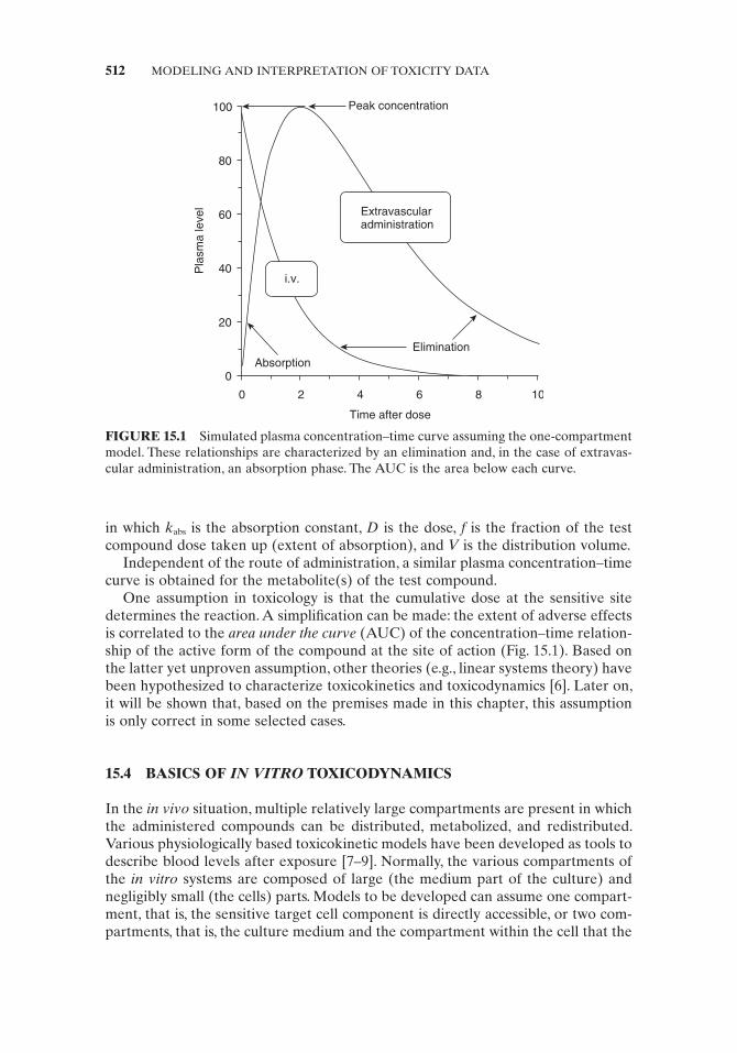
After an extravascular administration, the compound fi rst has to enter the circu-lation before it is eliminated from this compartment. The delay and magnitude of the peak plasma concentration following extravascular administration are a func-tion of the kinetics of absorption as well as, in the case of inhalation and oral administration, the fraction ( f ) of the absorbed unchanged compound (Fig. 15.1 ). The value of f normally equals 1 for an extravascular injection of the compound (IM, SC, IP) but is lower than 1 after an oral intake or after inhalation. The volume of distribution V is strongly compound dependent and may generally vary between 0.1 and 10 L/kg body weight.
The equation for the concentration of the test compound y i in the blood serum assuming one compartment corresponds to the Bateman equation [1] :
y
DfV
ke e
k ki
k t k ti i
= ( ) −−
⎛⎝⎜
⎞⎠⎟
− −
absabs el
el abs
(15.3)
TOXICOKINETICS IN VIVO 511
512 MODELING AND INTERPRETATION OF TOXICITY DATA
in which k abs is the absorption constant, D is the dose, f is the fraction of the test compound dose taken up (extent of absorption), and V is the distribution volume.
Independent of the route of administration, a similar plasma concentration – time curve is obtained for the metabolite(s) of the test compound.
One assumption in toxicology is that the cumulative dose at the sensitive site determines the reaction. A simplifi cation can be made: the extent of adverse effects is correlated to the area under the curve (AUC) of the concentration – time relation-ship of the active form of the compound at the site of action (Fig. 15.1 ). Based on the latter yet unproven assumption, other theories (e.g., linear systems theory) have been hypothesized to characterize toxicokinetics and toxicodynamics [6] . Later on, it will be shown that, based on the premises made in this chapter, this assumption is only correct in some selected cases.
15.4 BASICS OF IN VITRO TOXICODYNAMICS
In the in vivo situation, multiple relatively large compartments are present in which the administered compounds can be distributed, metabolized, and redistributed. Various physiologically based toxicokinetic models have been developed as tools to describe blood levels after exposure [7 – 9] . Normally, the various compartments of the in vitro systems are composed of large (the medium part of the culture) and negligibly small (the cells) parts. Models to be developed can assume one compart-ment, that is, the sensitive target cell component is directly accessible, or two com-partments, that is, the culture medium and the compartment within the cell that the
FIGURE 15.1 Simulated plasma concentration – time curve assuming the one - compartment model. These relationships are characterized by an elimination and, in the case of extravas-cular administration, an absorption phase. The AUC is the area below each curve.
Extravascularadministration
i.v.
100
80
60
40
20
0Absorption
Elimination
0 2 4 6 8 10
Time after dose
Pla
sm
a level
Peak concentration
BASICS OF IN VITRO TOXICODYNAMICS 513
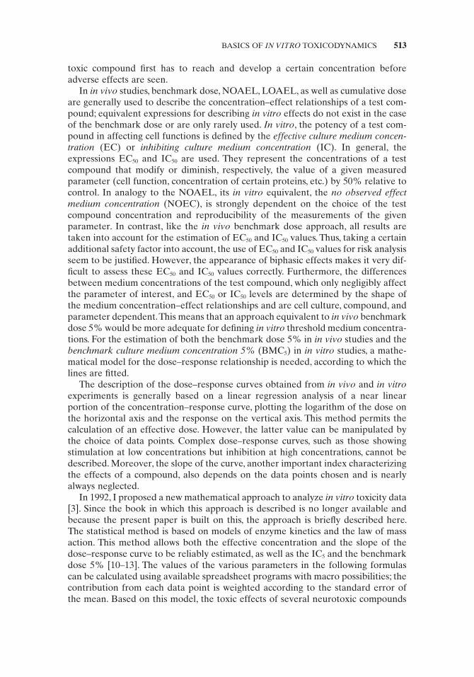
toxic compound fi rst has to reach and develop a certain concentration before adverse effects are seen.
In in vivo studies, benchmark dose, NOAEL, LOAEL, as well as cumulative dose are generally used to describe the concentration – effect relationships of a test com-pound; equivalent expressions for describing in vitro effects do not exist in the case of the benchmark dose or are only rarely used. In vitro , the potency of a test com-pound in affecting cell functions is defi ned by the effective culture medium concen-tration (EC) or inhibiting culture medium concentration (IC). In general, the expressions EC 50 and IC 50 are used. They represent the concentrations of a test compound that modify or diminish, respectively, the value of a given measured parameter (cell function, concentration of certain proteins, etc.) by 50% relative to control. In analogy to the NOAEL, its in vitro equivalent, the no observed effect medium concentration (NOEC), is strongly dependent on the choice of the test compound concentration and reproducibility of the measurements of the given parameter. In contrast, like the in vivo benchmark dose approach, all results are taken into account for the estimation of EC 50 and IC 50 values. Thus, taking a certain additional safety factor into account, the use of EC 50 and IC 50 values for risk analysis seem to be justifi ed. However, the appearance of biphasic effects makes it very dif-fi cult to assess these EC 50 and IC 50 values correctly. Furthermore, the differences between medium concentrations of the test compound, which only negligibly affect the parameter of interest, and EC 50 or IC 50 levels are determined by the shape of the medium concentration – effect relationships and are cell culture, compound, and parameter dependent. This means that an approach equivalent to in vivo benchmark dose 5% would be more adequate for defi ning in vitro threshold medium concentra-tions. For the estimation of both the benchmark dose 5% in in vivo studies and the benchmark culture medium concentration 5% (BMC 5 ) in in vitro studies, a mathe-matical model for the dose – response relationship is needed, according to which the lines are fi tted.
The description of the dose – response curves obtained from in vivo and in vitro experiments is generally based on a linear regression analysis of a near linear portion of the concentration – response curve, plotting the logarithm of the dose on the horizontal axis and the response on the vertical axis. This method permits the calculation of an effective dose. However, the latter value can be manipulated by the choice of data points. Complex dose – response curves, such as those showing stimulation at low concentrations but inhibition at high concentrations, cannot be described. Moreover, the slope of the curve, another important index characterizing the effects of a compound, also depends on the data points chosen and is nearly always neglected.
In 1992, I proposed a new mathematical approach to analyze in vitro toxicity data [3] . Since the book in which this approach is described is no longer available and because the present paper is built on this, the approach is briefl y described here. The statistical method is based on models of enzyme kinetics and the law of mass action. This method allows both the effective concentration and the slope of the dose – response curve to be reliably estimated, as well as the IC 5 and the benchmark dose 5% [10 – 13] . The values of the various parameters in the following formulas can be calculated using available spreadsheet programs with macro possibilities; the contribution from each data point is weighted according to the standard error of the mean. Based on this model, the toxic effects of several neurotoxic compounds
514 MODELING AND INTERPRETATION OF TOXICITY DATA
have been evaluated [14 – 18] . Recently, other very similar approaches have been suggested [19] .
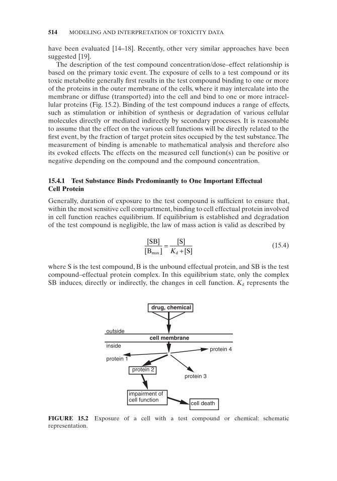
The description of the test compound concentration/dose – effect relationship is based on the primary toxic event. The exposure of cells to a test compound or its toxic metabolite generally fi rst results in the test compound binding to one or more of the proteins in the outer membrane of the cells, where it may intercalate into the membrane or diffuse (transported) into the cell and bind to one or more intracel-lular proteins (Fig. 15.2 ). Binding of the test compound induces a range of effects, such as stimulation or inhibition of synthesis or degradation of various cellular molecules directly or mediated indirectly by secondary processes. It is reasonable to assume that the effect on the various cell functions will be directly related to the fi rst event, by the fraction of target protein sites occupied by the test substance. The measurement of binding is amenable to mathematical analysis and therefore also its evoked effects. The effects on the measured cell function(s) can be positive or negative depending on the compound and the compound concentration.
15.4.1 Test Substance Binds Predominantly to One Important Effectual Cell Protein
Generally, duration of exposure to the test compound is suffi cient to ensure that, within the most sensitive cell compartment, binding to cell effectual protein involved in cell function reaches equilibrium. If equilibrium is established and degradation of the test compound is negligible, the law of mass action is valid as described by
[ ][ ]
[ ][ ]max
SBB
SSd
=+K
(15.4)
where S is the test compound, B is the unbound effectual protein, and SB is the test compound – effectual protein complex. In this equilibrium state, only the complex SB induces, directly or indirectly, the changes in cell function. K d represents the
FIGURE 15.2 Exposure of a cell with a test compound or chemical: schematic representation.
drug, chemical
cell membrane
protein 1
protein 2protein 3
protein 4
impairment of cell function
cell death
outside
inside
BASICS OF IN VITRO TOXICODYNAMICS 515
equilibrium dissociation constant. The total amount of protein [ B max ] is the sum of [B] and [SB]. [SB]/[B max ] is the fraction of effectual protein sites to which the test compound is bound. If the relationship between the fraction of bound sites and the changes in the cell function(s) being measured is linear, then Eq. 15.4 can be rewrit-ten to incorporate the cell function:
EE K
i
u r
SS
=+
[ ][ ]
(15.5)
where E u is the experimental value of the cell function in untreated cells, E i is the reduction in E u caused by the test substance, and K r is the response constant of the cell for the test substance.
The value of cell function of interest in the presence of the test substance as a fraction of the value of the cell function in untreated cells ( E t / E u ) is, therefore
EE
KK
t
u
r
r S=
+ [ ] (15.6)
where E t is the measured value of the cell function in treated cells and E u = E t + E i .
Generally, the toxic effects are expressed by IC 50 or BMC 5 . With this equation, IC 50 and BMC 5 can be calculated. As defi ned previously, IC 50 is the concentration of the test substance when the measured value of cell function is reduced to half its maximum value: E t / E u = 0.5 (see Fig. 15.3 : N c = 1). Thus,
0 5
5050. =
+=
KK
Kr
rr
ICor IC
(15.7)
The BMC 5 is defi ned as the concentrations where E t / E u = 0.95. Thus,
BMC
19r
5 =K
(15.8)
If in Eq. 15.8 K r is replaced by IC 50 , then according to Eq. 15.7 BMC 5 can be related to IC 50 as follows:
BMC
IC19
550=
(15.9)
In most cases, however, the effect on the cell function(s) of the binding of the test substance to the relevant effectual protein is not linearly related to the fraction of bound effectual protein sites ([SB]/[B max ] ). Generally, as the number of occupied sites increases, the effect on the measured cell function will be enhanced with every additional occupied site. Thus, as [S] increases, K r decreases. In other words, a posi-tive cooperativity analogous to the binding of oxygen to hemoglobin as described by Hill [2] is observed. Therefore,
516 MODELING AND INTERPRETATION OF TOXICITY DATA
EE i
KK
KK
KK
i
i
t
u
r
r
r
r
r
rS S S=
++
++ +
+⎛⎝
⎞⎠
1 1
1
2
2[ ] [ ] [ ]�
in which i is the number of effectual protein molecules or, more generally,
EE
KK N
t
u
c
c S c=
+ [ ] (15.10)
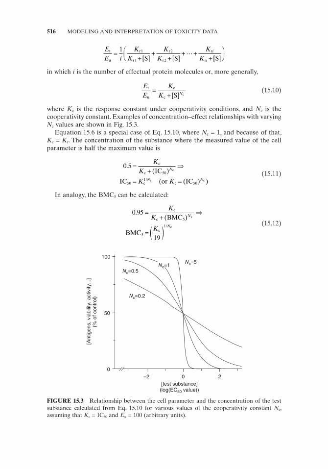
where K c is the response constant under cooperativity conditions, and N c is the cooperativity constant. Examples of concentration – effect relationships with varying N c values are shown in Fig. 15.3 .
Equation 15.6 is a special case of Eq. 15.10 , where N c = 1, and because of that, K c = K r . The concentration of the substance where the measured value of the cell parameter is half the maximum value is
0 550
501
50
.( )
( ( ) )
=+
⇒
= =
KK
K K
N
N N
c
c
c/
c
IC
IC or IC
c
c c
(15.11)
In analogy, the BMC 5 can be calculated:
0 95
19
5
5
1
.( )
=+
⇒
= ( )
KK
K
N
N
c
c
c/
BMC
BMC
c
c
(15.12)
FIGURE 15.3 Relationship between the cell parameter and the concentration of the test substance calculated from Eq. 15.10 for various values of the cooperativity constant N c , assuming that K c = IC 50 and E u = 100 (arbitrary units).
100
50
0
[Antigens, via
bili
ty, activity...]
(% o
f contr
ol) Nc=0.2
Nc=0.5Nc=1
Nc=5
–2 0 2
[test substance](log(EC50 value))

BASICS OF IN VITRO TOXICODYNAMICS 517
Small variations of N c strongly affect the BMC 5 value. In analogy to Eq. 15.9 , by combining Eqs. 15.11 and 15.12 , the BMC 5 in relation to N c and IC 50 can be described by the following equation:
BMC
IC/ c
550
119=
N
(15.13)
By reducing N c values, the ratio IC 50 /BMC 5 increases exponentially. Thus, small variations of N c value affect the BMC 5 value maximally at very small N c .
The distribution of the logarithm of the IC 50 and BMC 5 values found under experimental conditions is (as stated for the in vivo situation [20] ) log - normal Gaussian around the mean of the logarithm of the IC 50 and BMC 5 values, respec-tively, for each experiment and not (as suggested by others [19] ) normal at the nonlogarithmic linear scale. The same appears to be true for the N c values.
15.4.2 Test Substance Binds to Two Important Effectual Proteins with Different Affi nities
After application of a compound under the present assumption, two different main effects on cells can be discriminated depending on the applied concentration. In this case, E t / E u represents a combination of the effects induced by effectual protein 1 with parameters E u1 , K c1 , and N c1 and by effectual protein 2 with parameters E u2 , K c2 , and N c2 . Thus,
EE
E KK
E KK
E E
N Nt
u
u c
c
u c
c
u u
S Sc c
= ++
++
1 1
1
2 2
2
1 2
1 2[ ] [ ]
(15.14)
where
E E Eu u u= +1 2 (15.15)
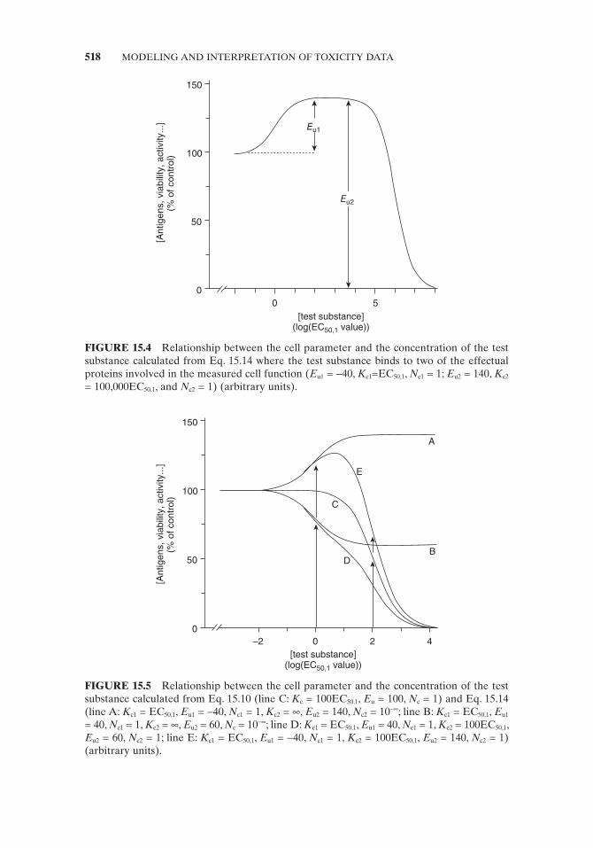
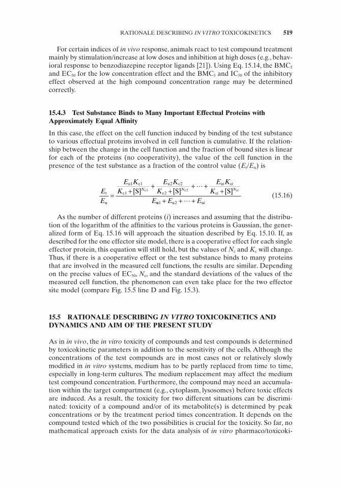
For both phases of the medium concentration – effect relationship, BMC 5 values can be calculated. Binding of the test substance to the effectual proteins can stimu-late or inhibit cell function. In case that binding to effectual protein 1 stimulates cell function and binding to effectual protein 2 inhibits cell function, the value of E u2 will represent the sum of the control value and the increase induced by binding to effectual protein 1 (Fig. 15.4 ) where E u1 has a negative value. Instead of IC 50 , the more general term effective concentration 50% (EC 50 ) is used to describe the con-centration resulting in a 50% stimulation or inhibition. Examples of both situations, namely, where both E u values are positive or one is positive and one is negative, are shown in Figs. 15.4 and 15.5 (line D in Fig. 15.5 is the sum of B and C, and line E is the sum of A and C). Equation 15.14 also applies if a test substance in the concen-tration range investigated only affects a fraction of the measured functional param-eter (Fig. 15.4 in the concentration range 0 – 1000EC 50,1 , and Fig. 15.5 lines A and B). In this case, the IC 50 value for binding to the second protein is outside the tested concentration range and the cooperativity constant N c must be set to 10 − ∞ .
518 MODELING AND INTERPRETATION OF TOXICITY DATA
FIGURE 15.4 Relationship between the cell parameter and the concentration of the test substance calculated from Eq. 15.14 where the test substance binds to two of the effectual proteins involved in the measured cell function ( E u1 = − 40, K c1 =EC 50,1 , N c1 = 1; E u2 = 140, K c2 = 100,000EC 50,1 , and N c2 = 1) (arbitrary units).
150
100
50
0
[Antigens, via
bili
ty, activity...]
(% o
f contr
ol)
0 5
[test substance](log(EC50,1 value))
Eu2
Eu1
FIGURE 15.5 Relationship between the cell parameter and the concentration of the test substance calculated from Eq. 15.10 (line C: K c = 100EC 50,1 , E u = 100, N c = 1) and Eq. 15.14 (line A: K c1 = EC 50,1 , E u1 = − 40, N c1 = 1, K c2 = ∞ , E u2 = 140, N c2 = 10 − ∞ ; line B: K c1 = EC 50,1 , E u1 = 40, N c1 = 1, K c2 = ∞ , E u2 = 60, N c = 10 − ∞ ; line D: K c1 = EC 50,1 , E u1 = 40, N c1 = 1, K c2 = 100EC 50,1 , E u2 = 60, N c2 = 1; line E: K c1 = EC 50,1 , E u1 = − 40, N c1 = 1, K c2 = 100EC 50,1 , E u2 = 140, N c2 = 1) (arbitrary units).
150
100
50
0
[Antigens, via
bili
ty, activity...]
(% o
f contr
ol)
–2 0 2 4
[test substance](log(EC50,1 value))
E
C
DB
A
For certain indices of in vivo response, animals react to test compound treatment mainly by stimulation/increase at low doses and inhibition at high doses (e.g., behav-ioral response to benzodiazepine receptor ligands [21] ). Using Eq. 15.14 , the BMC 5 and EC 50 for the low concentration effect and the BMC 5 and IC 50 of the inhibitory effect observed at the high compound concentration range may be determined correctly.
15.4.3 Test Substance Binds to Many Important Effectual Proteins with Approximately Equal Affi nity
In this case, the effect on the cell function induced by binding of the test substance to various effectual proteins involved in cell function is cumulative. If the relation-ship between the change in the cell function and the fraction of bound sites is linear for each of the proteins (no cooperativity), the value of the cell function in the presence of the test substance as a fraction of the control value ( E t / E u ) is
EE
E KK
E KK
E KK
E
N Ni i
iN i
t
u
u c
c
u c
c
u c
cS S Sc c c
= ++
++ +
+1 1
1
2 2
21 2[ ] [ ] [ ]
�
uu u u1 2+ + +E E i� (15.16)
As the number of different proteins ( i ) increases and assuming that the distribu-tion of the logarithm of the affi nities to the various proteins is Gaussian, the gener-alized form of Eq. 15.16 will approach the situation described by Eq. 15.10 . If, as described for the one effector site model, there is a cooperative effect for each single effector protein, this equation will still hold, but the values of N c and K c will change. Thus, if there is a cooperative effect or the test substance binds to many proteins that are involved in the measured cell functions, the results are similar. Depending on the precise values of EC 50 , N c , and the standard deviations of the values of the measured cell function, the phenomenon can even take place for the two effector site model (compare Fig. 15.5 line D and Fig. 15.3 ).
15.5 RATIONALE DESCRIBING IN VITRO TOXICOKINETICS AND DYNAMICS AND AIM OF THE PRESENT STUDY
As in in vivo , the in vitro toxicity of compounds and test compounds is determined by toxicokinetic parameters in addition to the sensitivity of the cells. Although the concentrations of the test compounds are in most cases not or relatively slowly modifi ed in in vitro systems, medium has to be partly replaced from time to time, especially in long - term cultures. The medium replacement may affect the medium test compound concentration. Furthermore, the compound may need an accumula-tion within the target compartment (e.g., cytoplasm, lysosomes) before toxic effects are induced. As a result, the toxicity for two different situations can be discrimi-nated: toxicity of a compound and/or of its metabolite(s) is determined by peak concentrations or by the treatment period times concentration. It depends on the compound tested which of the two possibilities is crucial for the toxicity. So far, no mathematical approach exists for the data analysis of in vitro pharmaco/toxicoki-
RATIONALE DESCRIBING IN VITRO TOXICOKINETICS 519
520 MODELING AND INTERPRETATION OF TOXICITY DATA
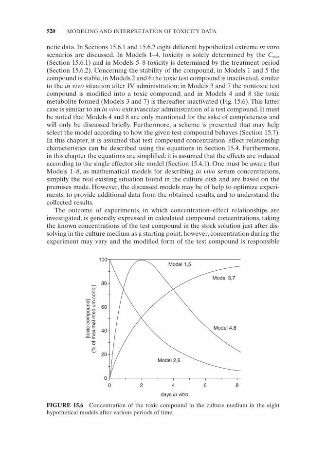
netic data. In Sections 15.6.1 and 15.6.2 eight different hypothetical extreme in vitro scenarios are discussed. In Models 1 – 4 , toxicity is solely determined by the C max (Section 15.6.1 ) and in Models 5 – 8 toxicity is determined by the treatment period (Section 15.6.2 ). Concerning the stability of the compound, in Models 1 and 5 the compound is stable; in Models 2 and 6 the toxic test compound is inactivated, similar to the in vivo situation after IV administration; in Models 3 and 7 the nontoxic test compound is modifi ed into a toxic compound; and in Models 4 and 8 the toxic metabolite formed ( Models 3 and 7 ) is thereafter inactivated (Fig. 15.6 ). This latter case is similar to an in vivo extravascular administration of a test compound. It must be noted that Models 4 and 8 are only mentioned for the sake of completeness and will only be discussed briefl y. Furthermore, a scheme is presented that may help select the model according to how the given test compound behaves (Section 15.7 ). In this chapter, it is assumed that test compound concentration – effect relationship characteristics can be described using the equations in Section 15.4 . Furthermore, in this chapter the equations are simplifi ed: it is assumed that the effects are induced according to the single effector site model (Section 15.4.1 ). One must be aware that Models 1 – 8 , as mathematical models for describing in vivo serum concentrations, simplify the real existing situation found in the culture dish and are based on the premises made. However, the discussed models may be of help to optimize experi-ments, to provide additional data from the obtained results, and to understand the collected results.
The outcome of experiments, in which concentration – effect relationships are investigated, is generally expressed in calculated compound concentrations, taking the known concentrations of the test compound in the stock solution just after dis-solving in the culture medium as a starting point; however, concentration during the experiment may vary and the modifi ed form of the test compound is responsible
FIGURE 15.6 Concentration of the toxic compound in the culture medium in the eight hypothetical models after various periods of time.
100
80
60
40
20
0
0 2 4 6 8
days in vitro
[toxic
com
pound]
(% o
f m
axim
al m
ediu
m c
onc.)
Model 2,6
Model 4,8
Model 3,7
Model 1,5
for the observed adverse effects. Because of these reasons, instead of concentra-tion – effect relationship, the term initial outer compartment (cell culture medium) test compound concentration – effect relationship (OCER) is used. Furthermore, the cal-culated initial (starting) concentration of the compound causing certain effects is based on the compound concentration in the stock solution and is called the effec-tive initial concentration (EIC). In EIC z , z stands for the observed effect relative to control. Here, z is 50 if at the end of the treatment period, the value of the parameter of interest is exactly between the value of (untreated) controls and the maximal possible change. EIC 50 is thereby the starting (initial) concentration at which, at the end of the treatment period, this 50% reduction (or stimulation) occurs. In analogy, in BMC 5 z is 5 and represents a 5% change relative to control values. One possibility to determine the velocity of activation or inactivation of a test compound in the cell cultures is to modify the treatment schedules in such a way that the C max ( Models 1 – 4 ) and AUC ( Models 5 – 8 ) of the toxic compound or of its toxic metabolite are changed. These modifi cations in the treatment schedule include (a) a partial replace-ment of the culture medium by fresh culture medium not containing any compound ( compound dilution ) during the treatment period; (b) a partial replacement of the culture medium during the treatment period by fresh culture medium containing the compound at the initial concentration ( compound replacement ); and (c) a pre-incubation of the compound of interest at nearly the fi nal concentration before adding to the cell cultures ( compound preincubation ).
As mentioned above, schedules (a) and (b) normally occur if cultures are treated or kept for prolonged periods of time. In some labs, stock solutions of test com-pounds are made and kept until use. In that case, treatment schedule (c) takes place even if the person involved is unaware of it. This chapter takes these situations into account and even makes use of it. Models 1 – 4 are based on the assumption that the test compound does not penetrate into the cells (or, in the case where it is taken up, the test compound does not interact with intracellular components) and exerts its infl uence by interacting with components of the cell membrane: that is, a change in C max will result in a change in EIC z values (one - compartment models). In contrast, Models 5 – 8 are based on the assumption that the test compound fi rst has to pene-trate into the cells and exert its infl uence by interacting with an intracellular com-ponent; that is, the AUC and/or shape of the AUC will result in a change in EIC z values (two - compartment models). The observed differences in EIC z values in rela-tion to experiments in which no compound dilution, replacement, and preincubation are performed (termed control experiments ) are used as a base for the assessment of the test compound activation ( k met ) and/or inactivation ( k el ) constants. In this case test compound activation means modifi cation of the test compound in a way that the resulting modifi ed test compound is toxic. The opposite is meant with inactivation.
15.6 IN VITRO TOXICOKINETICS AND DYNAMICS
15.6.1 Effects Based on Peak Concentrations (One - Compartment Models)
Certain classes of compound either cannot overcome the cell membrane or they specifi cally interact with components of the outer cell membrane like receptors and
IN VITRO TOXICOKINETICS AND DYNAMICS 521
522 MODELING AND INTERPRETATION OF TOXICITY DATA
ion channels. In this case, the reaction occurs if enough test compound binds to the receptive membrane component. The threshold treatment period is assumed to be the time needed to reach equilibrium. The presumption is made that the latter period is negligible and is therefore not taken into account in Models 1 – 4 .
Model 1: The Compound Is Stable In this model the concentration of the test compound does not vary during the treatment period. The medium compound concentration at the end of the treatment period corresponds to the initial concen-tration at the beginning of the treatment period. Since the maximum medium con-centration is assumed to be the effective compound concentration, a compound dilution, such as occurs as a result of feeding the cultures by replacing old medium with fresh culture medium without test compound during the treatment period, or a compound preincubation before addition will not affect or shift the effective initial medium compound concentration (EIC) – response curves (OCERs).
Model 2: The Toxic Compound Is Inactivated In vitro , compounds are inactivated (eliminated) on the one hand by the cultured cells, or on the other hand extracellu-larly by decomposition, by reducing the cellular accessibility, such as binding to released products of the cultured cells or by interaction with medium constituents (mainly proteins). The half - life of the compound due to intracellular inactivation and extracellular inactivation as a result of the interaction with released products is determined by the cell density and the cellular activity. Since the volume of the culture medium relative to the number of cells is extremely large, of the three inac-tivation pathways, the effect of inactivation by cells or their products is mainly negligible. The inactivation due to decomposition is exponential with a constant half - life. The half - life of the test compound that is inactivated by interaction with medium constituents depends on the medium concentrations of these constituents. A nearly constant half - life will only be found at small test compound concentrations relative to the concentration of these constituents; otherwise the half - life will increase exponentially with time.
Due to the inactivation of the test compound, its maximum concentration is present at the moment of addition of the test compound to the cultures. Therefore, a dilution of the culture medium after addition will not affect the OCERs. The maximum medium concentration will only be reduced in the case of compound preincubation, but only if the test compound is inactivated by decomposition or by interaction with medium constituents and not by cell - related processes.
Assuming one compartment and a single treatment of the cultures, the culture medium concentration of the toxic compound ( y i ) follows the OCER as the one described for blood concentrations after an IV administration in vivo under the same assumptions. Thus, Eqs. 15.1 and 15.2 are also applicable for the present model for describing the culture medium concentration and the inactivation half - life, respectively.
After preincubation, less toxic compound will be present, resulting in an apparent shift in the OCER in which the effect is related to the test compound at the moment before preincubation was started (initial or starting concentration, EIC). Comparing EIC 50 values as calculated by Eq. 15.11 , an inactivation of 50% of the compound implies that, before preincubation, twice the concentration had to be present to give the same concentrations at the moment that the dilutions are added to the cultures and thus in concentrations giving the same effect. The presence of equal effects
implies that at the beginning of the treatment period equal toxic compound concen-trations were present in the cell cultures. An increase in EICz as result of preincuba-tion can be explained by a partial conversion of the toxic compound into a non-toxic substance. For example if 50% is inactivated during the preincubation period twice the concentration is needed to have at start of the treatment the same concentration of toxic compound. This can be described by the following equation,
EIC EIC el pz z
k te1 2= ⋅ − (15.17)
where k el is the elimination constant in the culture medium, t p is the preincubation duration (difference between the time point at which the preincubation was started and t 0 ), EIC z 1 is the obtained EIC z in experiments without compound preincubation, and EIC z 2 is the EIC z in experiments with compound preincubation.
The k el can be calculated with the following equation, which is obtained by rear-ranging Eq. 15.17 :
k
tz
zel
p
EICEIC
=−⎛
⎝⎜⎞⎠⎟
⎛⎝
⎞⎠
1 1
2
ln
(15.18)
Model 3: The Nontoxic Compound Is Modifi ed into a Toxic Compound This model describes the concentration and effects of those test compounds that are bioactivated as a result of an interaction with components of the culture medium. Effects of biotransformation by a rate - limiting process inside the cells or at the cell surface are not described by this model but are by Model 5 (Section 15.6.2 ). Although a nontoxic test compound may give rise to a range of products, each of them having different toxic effects, generally one product dominates in its toxic effects on the cell culture. The formation of this main important toxic product is subjected to the same kind of processes as described for inactivation of the test compound ( Model 2 ). The only difference is that in Model 3 the product is the toxic compound and in Model 2 the product is the original test compound. If one molecule of test com-pound gives rise to one toxic molecule, the concentration of the toxic product can be calculated by subtracting the concentration of the test compound at time t i from the initial test compound concentration at time t 0 . Otherwise, the test compound concentrations need to be multiplied by a factor representing the largest number of toxic molecules that are obtained from one molecule of test compound. The concentration of toxic product ( A i ) increases with treatment period ( t i ) (see Eq. 15.1 ) and is
A A eik ti= − −
0 1( )met (15.19)
where A 0 is the fi nal concentration of the toxic product when all test compound is bioactivated, A i is the concentration of the toxic product at t i , and k met is the rate constant of activation ( met abolism) [1] .
Like the elimination half - life, the rate of bioactivation can also be expressed in a “ half - life period ” defi ned as the time needed to activate half of the test compound. Thus, A A A ei
k t= = − −0 5 10 0. ( )met 1/2 and, in analogy to Eq. 15.2 ,
t
k1/2
met
=ln( )2
(15.20)
IN VITRO TOXICOKINETICS AND DYNAMICS 523
524 MODELING AND INTERPRETATION OF TOXICITY DATA
Although the nontoxic test compound only evokes toxic effects by its toxic product(s), the extent of toxic effects is related to the concentration of the nontoxic compound added to the culture medium. This characteristic can be used to assess k met experimentally without measuring the concentrations in the culture medium. The k met can be calculated if results from the control experiment are compared with data from experiments using compound dilution, compound replacement, or com-pound preincubation.
compound dilution According to Eq. 15.19 , the concentration of the toxic product at the time point just before medium dilution ( t 1 ) corresponds to
A A e k t1 0 1 1= − −( )met (15.21)
and at the end of the treatment period after dilution of the medium by a factor x to
A
A ex
i
k ti
=− −
0 1( )met
(15.22)
By comparing data obtained from dilution and control experiments, the following scenarios may occur:
1. The medium is diluted by test compound - free medium after full activation of the test compound in the cell cultures. Under these circumstances, the concen-tration – response curve will not be affected by the dilution.
2. The medium is diluted by test compound - free medium before the test com-pound is fully activated in the cell cultures. (a) The dilution factor and/or t 1 is large enough that A 1 > A i . Under these
conditions, identical maximum concentrations and thus effects are obtained if
A e A ek t k ti01 021 1 1( ) ( )− = −− −met met
where
A 01 is the initial, starting concentration of the test compound in experi-ments without dilution and A 02 is the initial, starting concentration of the test compound in experiments with dilution.
If the maximum concentrations that are reached in culture medium during cell treatment are directly correlated with the resulting cellular effects,
AA
z
z
01
02
1
2
=EICEIC
(15.23)
Thus,
EICEIC
met
met
z
z
k t
k t
ee i
1
2
11
1
=−−
−
− (15.24)
k met can be calculated after fi lling in EIC z 1 , EIC z 2 , t 1 , and ti .
(b) The most common situation is that x is large and so A 1 < A i . Under these circumstances, identical maximum concentrations are obtained if
A e
A ex
k tk t
ii
01021
1( )
( )− =
−−−
metmet
where again x is the dilution factor (see Eqs. 15.21 and 15.22 ). Also, in combination with Eq. 15.23 and after some rearrangement,
EICEIC
z
z x1
2
1=
This implies that under these circumstances k met cannot be assessed.
compound replacement An analogue situation as described earlier occurs if the replacing medium contains the test compound at an identical concentration as present at t 0 . The EIC z in experiments with compound replacement will increase in comparison to control experiments. This will occur because at t 1 not only is the test compound replaced but the toxic product formed in the cultures is diluted by a factor x . No change or only a negligible change in EIC z will occur if the activation half - life is very small and at t 1 or t i the maximum concentration of the toxic metabo-lite is already present. A similar situation occurs if both x and t 1 are very large ( t 1 >> 0.5 t i ). The increase in EIC z value is maximum in the case where the concentra-tions of the toxic product at t 1 and t i are the same (i.e., after complete replacement t 1 = 0.5 t i ). In the latter situations, the maximum concentration of the toxic product is reached in the culture just before the compound replacement and Eq. 15.24 can be used for calculating k met . Otherwise, the following correlation between A 01 (Eq. 15.21 ) and A 02 (see Eq. 15.22 ) exists:
A e
A ex
x A ek tk t k t ti i
0102 021
1 1 11
1
( )( ) ( ) ( )( )
− =−
+− −−
− − −met
met met
xx
or in combination with Eq. 15.23
EICEIC
met met
met
z
z
k t k t t
k t
x e x ex e
i i1
2
11
1
1=
− + −−
− − −
−
( )( )
( )
Again, k met can be calculated after fi lling in EIC z 1 , EIC z 2 , x, t 1 , and t i .
compound preincubation If no full activation is achieved, the fi nal concentration A i of the activated compound is A e k t ti
0 1( )( )− − +met p instead of A e k ti0 1( )− − met after
inclusion of a preincubation period. To obtain identical concentrations at the end of the treatment period, the starting concentration must be comparably higher to the extent that
A e A ek t k t ti i01 021 1( ) ( )( )− = −− − +met met p
IN VITRO TOXICOKINETICS AND DYNAMICS 525
526 MODELING AND INTERPRETATION OF TOXICITY DATA
By assuming that the effects seen are directly dependent on the fi nal concentration of the bioactivated compound, we fi nd
EICEIC
met p
met
z
z
k t t
k t
ee
i
i
1
2
11
=−
−
− +
−
( )
in which EIC z 1 and EIC z 2 are the concentrations needed to obtain similar effects (EIC z 1 (controls) and EIC z 2 (experiment with compound preincubation) according to Eq. 15.19 and in combination with Eq. 15.23 ).
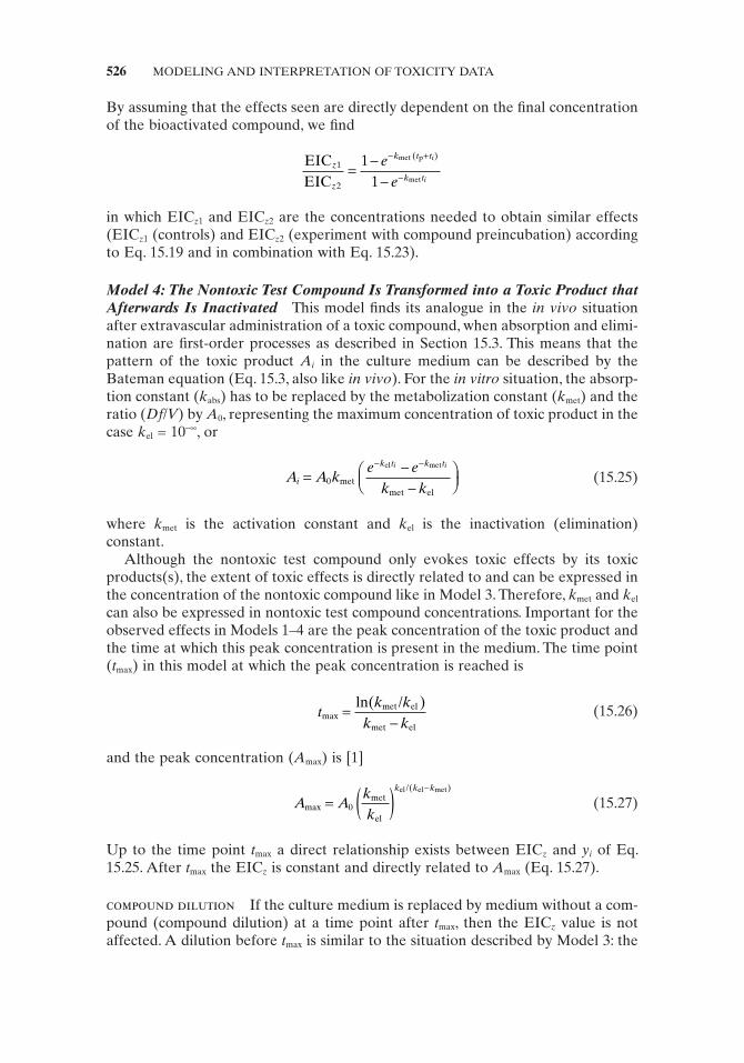
Model 4: The Nontoxic Test Compound Is Transformed into a Toxic Product that Afterwards Is Inactivated This model fi nds its analogue in the in vivo situation after extravascular administration of a toxic compound, when absorption and elimi-nation are fi rst - order processes as described in Section 15.3 . This means that the pattern of the toxic product A i in the culture medium can be described by the Bateman equation (Eq. 15.3 , also like in vivo ). For the in vitro situation, the absorp-tion constant ( k abs ) has to be replaced by the metabolization constant ( k met ) and the ratio ( Df / V ) by A 0 , representing the maximum concentration of toxic product in the case k el = 10 − ∞ , or
A A k
e ek k
i
k t k ti i
=−−
⎛⎝⎜
⎞⎠⎟
− −
0 metmet el
el met
(15.25)
where k met is the activation constant and k el is the inactivation (elimination) constant.
Although the nontoxic test compound only evokes toxic effects by its toxic products(s), the extent of toxic effects is directly related to and can be expressed in the concentration of the nontoxic compound like in Model 3 . Therefore, k met and k el can also be expressed in nontoxic test compound concentrations. Important for the observed effects in Models 1 – 4 are the peak concentration of the toxic product and the time at which this peak concentration is present in the medium. The time point ( t max ) in this model at which the peak concentration is reached is
t
k kk k
maxln( )
=−
met el
met el
/
(15.26)
and the peak concentration ( A max ) is [1]
A A
kk
k k k
max
( )
= ( ) −
0met
el
/el el met
(15.27)
Up to the time point t max a direct relationship exists between EIC z and y i of Eq. 15.25 . After t max the EIC z is constant and directly related to A max (Eq. 15.27 ).
compound dilution If the culture medium is replaced by medium without a com-pound (compound dilution) at a time point after t max , then the EIC z value is not affected. A dilution before t max is similar to the situation described by Model 3 : the
maximum concentration of toxic product is present in the culture medium at the end of the treatment period. Comparing data obtained from dilution and control experiments, the same scenarios may occur as in Model 3 . However, EIC z correlates with Eq. 15.25 and not with Eq. 15.19 . Since before t max A i can nearly be mimicked by Eq. 15.19 , in practice it will not be possible to discriminate between Model 3 and 4 under these circumstances using compound dilution experiments.
compound preincubation In analogy to compound dilution, the value of t max is decisive as to which effect a compound preincubation has on the EIC z value. Of the four different scenarios that can be discriminated, three are possible in practice: (1) The t max in both cases (with and without preincubation) has a value between t 0 and t i . In this scenario a compound preincubation has no effect on EIC z . (2). The t max is reached during the preincubation period. In this case a preincubation of the com-pound dilutions results in an increase in the EIC z value. The compound behaves very similarly to that described in Model 2 . (3) The t max is greater than t i , irrespective of the value of t p , or occurs only after preincubation. Under these circumstances, a compound preincubation results in a decrease in the EIC z value. The compound behaves as described in Model 3 . Since under possibilities (2) and (3) the OCER can be mimicked fairly well by the equations describing Models 2 and 3 , respectively, it is not possible to discriminate between these models and Model 4 under experi-mental conditions.
15.6.2 Effects Based on Accumulation (Two - Compartment Models)
Several compounds of different compound classes seem not to have an acute effect or only after extreme doses. Their toxicity seems to be dependent on the total cumulative dose received and not merely on the treatment schedule. Therefore, their effects seem to be related with the in vivo area under the serum concentration – time curve (AUC) (Fig. 15.1 ) and not by a single dose or by the maximum serum concentration.
The reason why one toxic compound at a given blood concentration is effective at a short exposure time while other compounds require a prolonged period of time to be effective is assumed to be the difference in the accessibility of the target protein(s) for the toxic test compound. Whereas some compounds introduced into a test system are obviously able to interact directly and freely with the target protein(s) resulting in acute effects, others are not. These latter compounds fi rst have to overcome some kind of “ barrier, ” which is not only determined by diffusion velocity. This barrier consists of saturable processes that limit transfer into the target compartment, such as carrier dependent transport, or saturable processes in which certain enzymes play a key role (formation of toxic product S * ; Fig. 15.7 ). In the latter case, a complex or a metabolite may be formed. In these kinds of barrier, accumulation is restricted by the number of interaction sites (binding sites). Binding site - limited processes can be described by the Michaelis – Menten relationship [22] :
vV K
0
max
[ ][ ]
=+S
Sm (15.28)
IN VITRO TOXICOKINETICS AND DYNAMICS 527
528 MODELING AND INTERPRETATION OF TOXICITY DATA
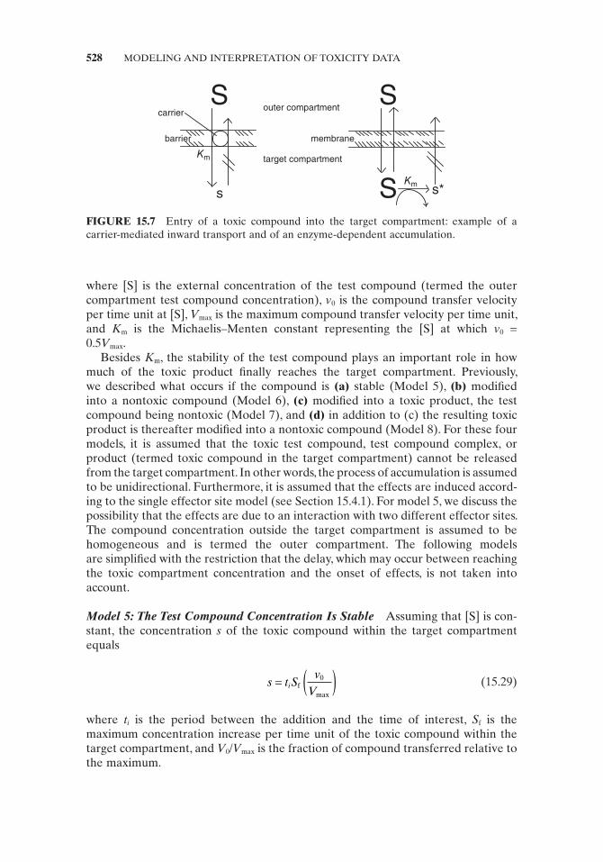
FIGURE 15.7 Entry of a toxic compound into the target compartment: example of a carrier - mediated inward transport and of an enzyme - dependent accumulation.
target compartment
outer compartmentS
s
Km
carrier
barrier
S
s*S
membrane
Km
where [S] is the external concentration of the test compound (termed the outer compartment test compound concentration), v 0 is the compound transfer velocity per time unit at [S], V max is the maximum compound transfer velocity per time unit, and K m is the Michaelis – Menten constant representing the [S] at which v 0 = 0.5 V max .
Besides K m , the stability of the test compound plays an important role in how much of the toxic product fi nally reaches the target compartment. Previously, we described what occurs if the compound is (a) stable ( Model 5 ), (b) modifi ed into a nontoxic compound ( Model 6 ), (c) modifi ed into a toxic product, the test compound being nontoxic ( Model 7 ), and (d) in addition to (c) the resulting toxic product is thereafter modifi ed into a nontoxic compound ( Model 8 ). For these four models, it is assumed that the toxic test compound, test compound complex, or product (termed toxic compound in the target compartment) cannot be released from the target compartment. In other words, the process of accumulation is assumed to be unidirectional. Furthermore, it is assumed that the effects are induced accord-ing to the single effector site model (see Section 15.4.1 ). For model 5 , we discuss the possibility that the effects are due to an interaction with two different effector sites. The compound concentration outside the target compartment is assumed to be homogeneous and is termed the outer compartment. The following models are simplifi ed with the restriction that the delay, which may occur between reaching the toxic compartment concentration and the onset of effects, is not taken into account.
Model 5: The Test Compound Concentration Is Stable Assuming that [S] is con-stant, the concentration s of the toxic compound within the target compartment equals
s t S
vV
i= ( )f0
max (15.29)
where t i is the period between the addition and the time of interest, S f is the maximum concentration increase per time unit of the toxic compound within the target compartment, and V 0 / V max is the fraction of compound transferred relative to the maximum.
The relationship between the outer compartment and target compartment con-centrations can be obtained by replacing the ratio v 0 / V max in Eq. 15.29 by Eq. 15.28 :
s t S
Ki=
+⎛⎝⎜
⎞⎠⎟f
m
SS
[ ][ ]
(15.30)
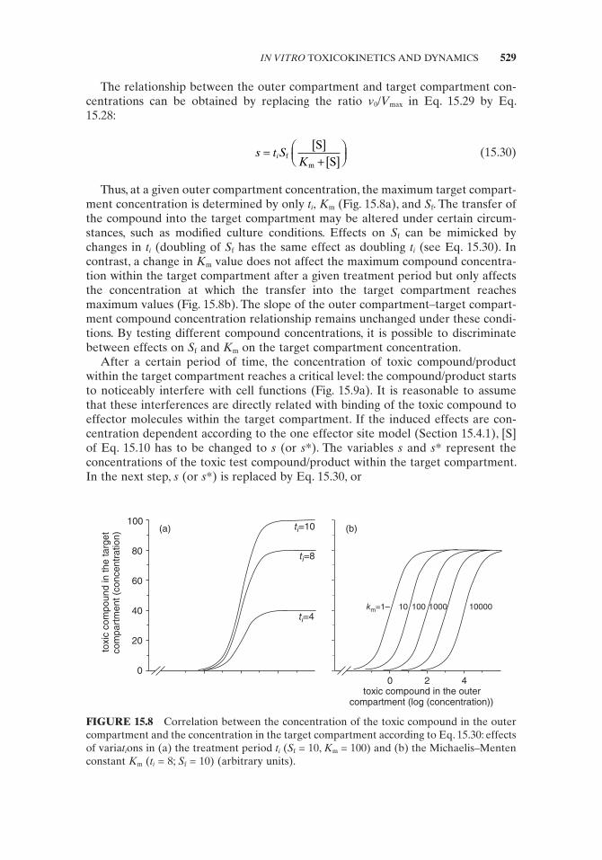
Thus, at a given outer compartment concentration, the maximum target compart-ment concentration is determined by only t i , K m (Fig. 15.8a ), and S f . The transfer of the compound into the target compartment may be altered under certain circum-stances, such as modifi ed culture conditions. Effects on S f can be mimicked by changes in t i (doubling of S f has the same effect as doubling t i (see Eq. 15.30 ). In contrast, a change in K m value does not affect the maximum compound concentra-tion within the target compartment after a given treatment period but only affects the concentration at which the transfer into the target compartment reaches maximum values (Fig. 15.8b ). The slope of the outer compartment – target compart-ment compound concentration relationship remains unchanged under these condi-tions. By testing different compound concentrations, it is possible to discriminate between effects on S f and K m on the target compartment concentration.
After a certain period of time, the concentration of toxic compound/product within the target compartment reaches a critical level: the compound/product starts to noticeably interfere with cell functions (Fig. 15.9a ). It is reasonable to assume that these interferences are directly related with binding of the toxic compound to effector molecules within the target compartment. If the induced effects are con-centration dependent according to the one effector site model (Section 15.4.1 ), [S] of Eq. 15.10 has to be changed to s (or s * ). The variables s and s * represent the concentrations of the toxic test compound/product within the target compartment. In the next step, s (or s * ) is replaced by Eq. 15.30 , or
FIGURE 15.8 Correlation between the concentration of the toxic compound in the outer compartment and the concentration in the target compartment according to Eq. 15.30 : effects of varia t i ons in (a) the treatment period t i ( S f = 10, K m = 100) and (b) the Michaelis – Menten constant K m ( t i = 8; S f = 10) (arbitrary units).
ti=10
ti=8
ti=4
100
80
60
40
20
0
toxic
com
pound in the targ
et
com
part
ment (c
oncentr
ation) (a) (b)
km=1– 10 100 1000 10000
0 2 4toxic compound in the outer
compartment (log (concentration))
IN VITRO TOXICOKINETICS AND DYNAMICS 529
530 MODELING AND INTERPRETATION OF TOXICITY DATA
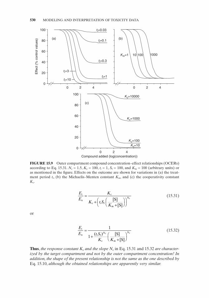
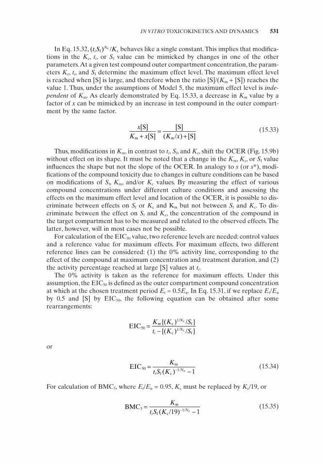
FIGURE 15.9 Outer compartment compound concentration – effect relationships (OCERs) according to Eq. 15.31 . N c = 1.5, K c = 100, t i = 1, S f = 100, and K m = 100 (arbitrary units) or as mentioned in the fi gure. Effects on the outcome are shown for variations in (a) the treat-ment period t i , (b) the Michaelis – Menten constant K m , and (c) the cooperativity constant K c .
ti=0.03
ti=0.1
ti=0.3
ti=3
ti=10ti=1
100
80
60
40
20
0
Effect (%
contr
ol valu
es) (a)
0 2 4
Kc=10000
Kc=1000
Kc=100
Kc=10
100
80
60
40
20
0
(c)
0 2 4
(b)
0 2 4
Km=1 10 100 1000
Compound added (log(concentration))
EE
K
K t SK
i
Nt
u
c
c fm
SS
c=
++
⎛⎝
⎞⎠
⎛⎝
⎞⎠
[ ][ ]
(15.31)
or
EE t S
K Ki
N Nt
u f
c m
c cSS
=+
+⎛⎝
⎞⎠
1
1( ) [ ]
[ ]
(15.32)
Thus , the response constant K c and the slope N c in Eq. 15.31 and 15.32 are character-ized by the target compartment and not by the outer compartment concentration! In addition, the shape of the present relationship is not the same as the one described by Eq. 15.10 , although the obtained relationships are apparently very similar.
In Eq. 15.32 , ( )t S KiN
f cc / behaves like a single constant. This implies that modifi ca-
tions in the K c , t i , or S f value can be mimicked by changes in one of the other parameters. At a given test compound outer compartment concentration, the param-eters K c , t i , and S f determine the maximum effect level. The maximum effect level is reached when [S] is large, and therefore when the ratio [S]/( K m + [S]) reaches the value 1. Thus, under the assumptions of Model 5 , the maximum effect level is inde-pendent of K m . As clearly demonstrated by Eq. 15.33 , a decrease in K m value by a factor of x can be mimicked by an increase in test compound in the outer compart-ment by the same factor.
xK x K x
[ ][ ]
[ ]( ) [ ]
SS
S/ Sm m+
=+
(15.33)
Thus, modifi cations in K m , in contrast to t i , S f , and K c , shift the OCER (Fig. 15.9b ) without effect on its shape. It must be noted that a change in the K m , K c , or S f value infl uences the shape but not the slope of the OCER. In analogy to s (or s * ), modi-fi cations of the compound toxicity due to changes in culture conditions can be based on modifi cations of S f , K m , and/or K c values. By measuring the effect of various compound concentrations under different culture conditions and assessing the effects on the maximum effect level and location of the OCER, it is possible to dis-criminate between effects on S f or K c and K m but not between S f and K c . To dis-criminate between the effect on S f and K c , the concentration of the compound in the target compartment has to be measured and related to the observed effects. The latter, however, will in most cases not be possible.
For calculation of the EIC 50 value, two reference levels are needed: control values and a reference value for maximum effects. For maximum effects, two different reference lines can be considered: (1) the 0% activity line, corresponding to the effect of the compound at maximum concentration and treatment duration, and (2) the activity percentage reached at large [S] values at t i .
The 0% activity is taken as the reference for maximum effects. Under this assumption, the EIC 50 is defi ned as the outer compartment compound concentration at which at the chosen treatment period E t = 0.5 E u . In Eq. 15.31 , if we replace E t / E u by 0.5 and [S] by EIC 50 , the following equation can be obtained after some rearrangements:
EIC
//
m c/
f
c/
f
c
c50
1
1=
−K K St K S
N
iN
{( ) }{( ) }
or
EIC m
f c/ c
50 1 1=
−−
Kt S Ki
N( ) (15.34)
For calculation of BMC 5 , where E t / E u = 0.95, K c must be replaced by K c /19, or
BMC
/m
f c/ c
5 119 1=
−−
Kt S Ki
N( ) (15.35)
IN VITRO TOXICOKINETICS AND DYNAMICS 531

532 MODELING AND INTERPRETATION OF TOXICITY DATA
Using this equation, N c , K m , and S f must be calculated by taking into account the activity percentage reached at large [S] values at the given t i . An example of such a relationship between EIC 50 and t i according to Eq. 15.34 is shown in Fig. 15.10 . A positive, fi ctitious value for EIC 50 is only obtained if t S Ki
Nf c
/ c( )−1 > 1. In this equa-tion, ( )K N
c/ c−1 represents the target compartment EIC 50 (see Eq. 15.11 ). Only if this
target compartment concentration is reached, can measurement of a 50% reduction be possible.
At short t i values, when t i S f values are near ( )K Nc
/ c1 , a doubling of t i will reduce EIC 50 much more than 50% due to the subtraction of 1 from t S Ki
Nf c
/ c( )−1 . Thus, the toxicity is not directly related to the AUC . If the compound concentration in the outer compartment is stable, the AUC after the treatment period t i is defi ned by
AUC AUC St t t ii i t= =⇒( ) [ ]0
where t i is the difference between the time at the end of the treatment period and the time at the beginning of the treatment period ( t 0 ).
At large t i the subtraction of 1 from t S KiN
f c/ c( )−1 will only marginally infl uence
the outcome. Only under these circumstances does a doubling of t i bisect the EIC 50 value or, in other words, EIC 50 / t i is constant. This implies that only at large t i can an inverse linear relationship exist between toxicity expressed by EIC 50 value and AUC.
If the results of two experiments are compared in which only t i was varied, an estimate of K m can be made if an inhibition of the parameter of interest of at least
FIGURE 15.10 Correlation between EIC 50 defi ned by 0% activity or by the activity per-centage reached if [S] = ∞ and treatment period t i . The effects are simulated according to the one effector site model (Eq. 15.34 and 15.39 , respectively) ( S f = 100, K c = 100,000, K m = 100, N c = 1.5) (arbitrary units).
4
2
0
0 1 2 3
log(ti)
log
(IC
50)
IC50/ti isconstant
Activity at [S]=∞is the reference
0% activity isthe reference
z % at maximum [S] is reached. The two different treatment periods are termed t i 1 and t i 2 . As a new variable, r is introduced representing the ratio r = ( t i 1 − t i 2 )/ t i 2 , or t i 1 = t i 2 (1 + r ). In Models 5 – 8 , the effects after t i 1 and t i 2 are the same if s 1 = s 2 , or
( )1 2
1
12
2
2
++{ } =
+{ }r t SK
t SK
iz
zi
z
zf
mf
m
EICEIC
EICEIC
where EIC z 1 and EIC z 2 are the initial outer compartment concentration after t i 1 and t i 2 , respectively, resulting in a reduction of the parameter of interest by z %. Or after rearrangement,
K
rrz z
z zm
EIC EICEIC EIC
=⋅ ⋅
− + ⋅1 2
2 11( ) (15.36)
Besides the possibility of calculating K m , this equation also indicates that a relation between treatment period and EIC z 1 and EIC z 2 exists, independent of S f , K c , and N c .
The reference for maximum effects is defi ned by the activity percentage reached at large [S] values. As mentioned before, at large [S] values the ratio [ S ]/( Km + [S]) in Eq. 15.31 reaches the value 1. Thus, the maximum possible effect level ( E tmax / E u ) after the given treatment period t i equals
EE
KK t Si N
t
u
c
c fc
max
( )=
+ (15.37)
The EIC 50 at the treatment period chosen under the present assumptions is defi ned as the outer compartment concentration at which
1 0 5 1− = −( )E
EE
Et
u
t
u
. max
(15.38)
In Eq. 15.38 , ( E t / E u ) can be replaced by Eq. 15.31 and ( E tmax / E u ) by Eq. 15.37 . After some rearrangements, the following is obtained:
EIC
/m
f c/c c
50 12 1=
+ −K
t S KiN N{ ( ) }
(15.39)
In analogy, the BMC 5 can be calculated:
1 0 05 1− = −( )E
EE
Et
u
t
u
. max
or
BMC
/m
f c/c c
5 120 19 1=
+ −K
t S KiN N{ ( ) }
(15.40)
IN VITRO TOXICOKINETICS AND DYNAMICS 533
534 MODELING AND INTERPRETATION OF TOXICITY DATA
As in the previous case, in which the 0% activity is taken as a reference, only at large t i can doubling of t i bisect the EIC 50 value. However, in contrast to the previous case, at very small t i a doubling of t i will reduce the EIC 50 value by less than 50%. This is due to the presence of the constant with a value of 2 in the denominator. Thus, again toxicity is inversely linearly correlated with the AUC only at large treat-ment periods (Fig. 15.10 ). Roughly, one can say that a linear relationship between AUC and EIC 50 exists as far as Eqs. 15.34 and 15.39 give similar EIC 50 values.
compound dilution If during the treatment period at a time t 1 the medium of the cultures is partially replaced by fresh medium without the test compound, the remaining compound is diluted, corresponding to the ratio of remaining old medium divided by total medium volume (factor x ). As a result, the increase in s per time unit is reduced after t 1 . Mathematically, the obtained OCER can be described by Eq. 15.32 , including an adaptation for the dilution of [S] at t 1 :
EE
K
K t SK
t t Sx
K xi
Ntdil
u
c
c fm
fm
SS
SS
c=
++{ } + −
+{ }⎛⎝
⎞⎠1 1
[ ][ ]
( )[ ]
[ ]
(15.41)
where E tdil and E u are values of the parameter of interest at the end of the treatment period, in which a dilution or no dilution step was carried out, respectively; t 1 S f {[S]/( K m + [S])} is the concentration of the test compound in the target compartment at the moment of dilution ( t 1 ), and ( t i − t 1 ) S f { x [S]/( K m + x [S])} is the increase of test com-pound in the target compartment from t 1 to the end of the treatment period ( t i ).
At large [S], however, the ratio x [S]/( K m + x [S]) is still near 1 except if x is extremely small (see Fig. 15.8 and Eq. 15.30 ). This implies that the same maximum effect level is obtained with or without compound dilution. Depending on the loca-tion of the maximum effect level at t 1 , two different situations can be discriminated after a compound dilution.
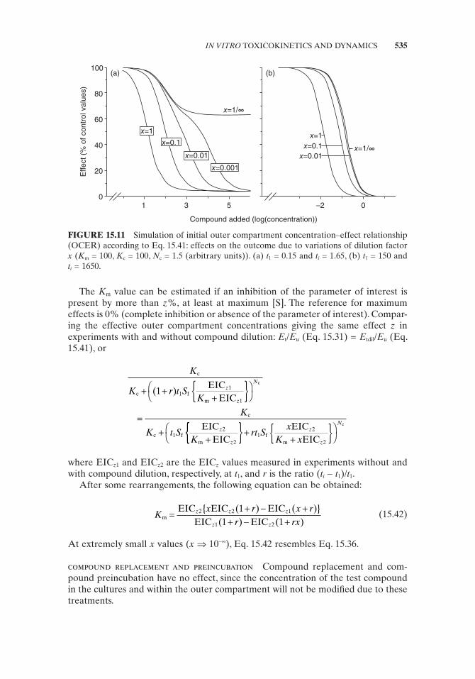
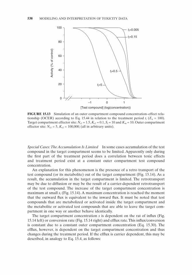
(a) The parameter of interest is completely inhibited at t 1 at maximum [S] values . With decreasing x values, the OCER found at t i will shift asymptotically toward the OCER measured at t 1 . No swallowed OCER will be obtained (Fig. 15.11 ). Independent of the value of t i , if x [S] is relatively small in com-parison to K m , then in ( t i − t 1 ) S f { x [S]/( K m + x [S])}, a decrease in the x value can be mimicked by an increase in t i and by that of t i − t 1 .
(b) Even at very large [S], s (or s * ) at t 1 is still too low to inhibit completely the parameter of interest . Only the part of the curve that represents the effect due to the treatment period to t 1 will behave in a similar way as described under (a). The other part will be shifted corresponding to the dilution. A dilution of 0.1 will shift the latter part of the relationship by a factor of 10, a dilution of 0.01 will result in a shift of a factor 100, and soon (see Fig. 15.11 ). At relatively large x values (0.01 – 1), only a change in the apparent N c will be observed and a swallowed OCER cannot be recognized. A complete removal of the compound at t 1 ( x = 10 − ∞ ) will result in an OCER correspond-ing to the effect of a treatment to t 1 . Thus, only under these extreme situations (complete removal) can a dilution of the compound be mimicked by a reduc-tion in the total treatment period without dilution!!
The K m value can be estimated if an inhibition of the parameter of interest is present by more than z %, at least at maximum [S]. The reference for maximum effects is 0% (complete inhibition or absence of the parameter of interest). Compar-ing the effective outer compartment concentrations giving the same effect z in experiments with and without compound dilution: E t / E u (Eq. 15.31 ) = E tdil / E u (Eq. 15.41 ), or
K
K r t SK
K
K t SK
z
z
N
z
z
c
c fm
c
c fm
EICEIC
EICEIC
c
+ ++{ }⎛
⎝⎞⎠
=+
+
( )1 11
1
12
2{{ } +
+{ }⎛⎝
⎞⎠rt S
xK x
z
z
N
12
2f
m
EICEIC
c
where EIC z 1 and EIC z 2 are the EIC z values measured in experiments without and with compound dilution, respectively, at t 1 , and r is the ratio ( t i − t 1 )/ t 1 .
After some rearrangements, the following equation can be obtained:
K
x r x rr rx
z z z
z zm
EIC EIC EICEIC EIC
=+ − +
+ − +2 2 1
1 2
11 1
{ ( ) ( )}( ) ( )
(15.42)
At extremely small x values ( x ⇒ 10 − ∞ ), Eq. 15.42 resembles Eq. 15.36 .
compound replacement and preincubation Compound replacement and com-pound preincubation have no effect, since the concentration of the test compound in the cultures and within the outer compartment will not be modifi ed due to these treatments.
FIGURE 15.11 Simulation of initial outer compartment concentration – effect relationship (OCER) according to Eq. 15.41 : effects on the outcome due to variations of dilution factor x ( K m = 100, K c = 100, N c = 1.5 (arbitrary units)). (a) t 1 = 0.15 and t i = 1.65, (b) t 1 = 150 and t i = 1650.
100
80
60
40
20
0
Effect (%
of contr
ol valu
es)
(a)
1 3 5
(b)
–2 0
x=1/∞
x=1/∞
x=1
x=0.1
x=0.01
x=0.001
x=0.01
x=0.1
x=1
Compound added (log(concentration))
IN VITRO TOXICOKINETICS AND DYNAMICS 535
536 MODELING AND INTERPRETATION OF TOXICITY DATA
Special Cases: Two or More Effector Sites Are Present If two or more effector sites are present, these various sites may be located in the same or in different target compartments.
(a) Both sites are located within the target compartment . The interaction between test compound and the main effector site need not always result in cell death. When numerous effector sites play a role in the observed effects, the resulting OCER can be described by Eq. 15.16 , replacing [S] by the s of Eq. 15.30 . The resulting equation is indistinguishable from Eq. 15.31 . Interactions of the test compound with two effector sites (the main and another effector site causing cell death) will result in swallowed or at least a less steep OCER. Mathematically, this OCER can be described by Eq. 15.14 , replacing [S] by the s (or s * ) of Eq. 15.30 . The latter substitu-tion results in the following equation:
EE
K E
K t SK
K E
K t SK
i
N
it
u
c u
c fm
c u
c fm
SS
Sc
=+
+{ }⎛⎝
⎞⎠
++
+
1 1
1
2 2
2
1[ ][ ]
[ ][[ ]S
c
u u
{ }⎛⎝
⎞⎠
+
N
E E
2
1 2 (15.43)
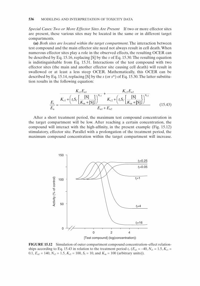
After a short treatment period, the maximum test compound concentration in the target compartment will be low. After reaching a certain concentration, the compound will interact with the high - affi nity, in the present example (Fig. 15.12 ) stimulatory, effector site. Parallel with a prolongation of the treatment period, the maximum compound concentration within the target compartment will increase.
FIGURE 15.12 Simulation of outer compartment compound concentration – effect relation-ships according to Eq. 15.43 in relation to the treatment period t i . ( E u1 = − 40, N c1 = 1.5, K c1 = 0.1, E u2 = 140, N c2 = 1.5, K c2 = 100, S f = 10, and K m = 100 (arbitrary units)).
0 2 4
[Test compound] (log(concentration))
Activity (
% o
f co
ntr
ol)
150
100
50
0
ti=0.25
ti=0.05
ti=1
ti=4
ti=16
The OCER of the fi rst effector site will shift to the left. In addition, other cell func-tions will be affected due to the interaction with the second effector site. With further prolongation of the treatment period, both OCERs will shift to the left. Since only the combined effects can be detected, this shift will be refl ected in a change in the overall shape of the outer culture medium concentration – response curve (Fig. 15.12 ).
(b) The two effector sites are located in different compartments . One of these compartments may represent a directly and freely accessible compartment, that is, the compartment to which the compound is added, and is termed the “ outer ” com-partment. The second compartment represents a compartment outside the latter compartment. The compound fi rst has to be transferred to this compartment and it is termed the “ target ” compartment. This implies that, as a result of an increase of the treatment period, only that part of the OCER will be shifted which is the result of the effector site being located within the target compartment. The other part of the OCER remains unaffected by a variation of the treatment period. If the various effector sites induce the same effect(s), their contributions for the observed effect(s) will change with the increase in treatment period. Otherwise, if the effector sites affect different functional parameters, the characteristics of the altered functional state of the cell will depend on the treatment period. With prolonged treatment periods, the effect induced by the effector site located in the outer compartment will be totally overshadowed by the effect induced by the other effector site(s) inside the target compartment . Often, two effects are characterized by different N c values. In this case, a treatment - period - dependent change in N c values will be observed. The sum of both effects can be characterized mathematically by multiplying Eq. 15.10 , which describes the treatment - period - independent effects, by Eq. 15.31 or 15.43, which describes the transfer - dependent effects. Since transfer - dependent and acute effects can be described according to the one site effector model, the OCER can be characterized by the following equation:
EE
K
K t SK
KK
i
Nt
u
c
c fm
c
cSS
Sc=
++{ }⎛
⎝⎞⎠
⎧
⎨⎪⎪
⎩⎪⎪
⎫
⎬⎪⎪
⎭⎪⎪
+1
1
2
21[ ]
[ ][ ]NNc 2{ }
(15.44)
in which effector site 1 (characterized by K c1 and N c1 ) is responsible for the transfer - dependent effects and effector site 2 (characterized by K c2 and N c2 ) is responsible for transfer - independent effects. In analogy, the same transition can be made if the transfer - dependent effects can be described according to the two effector site model (not shown).
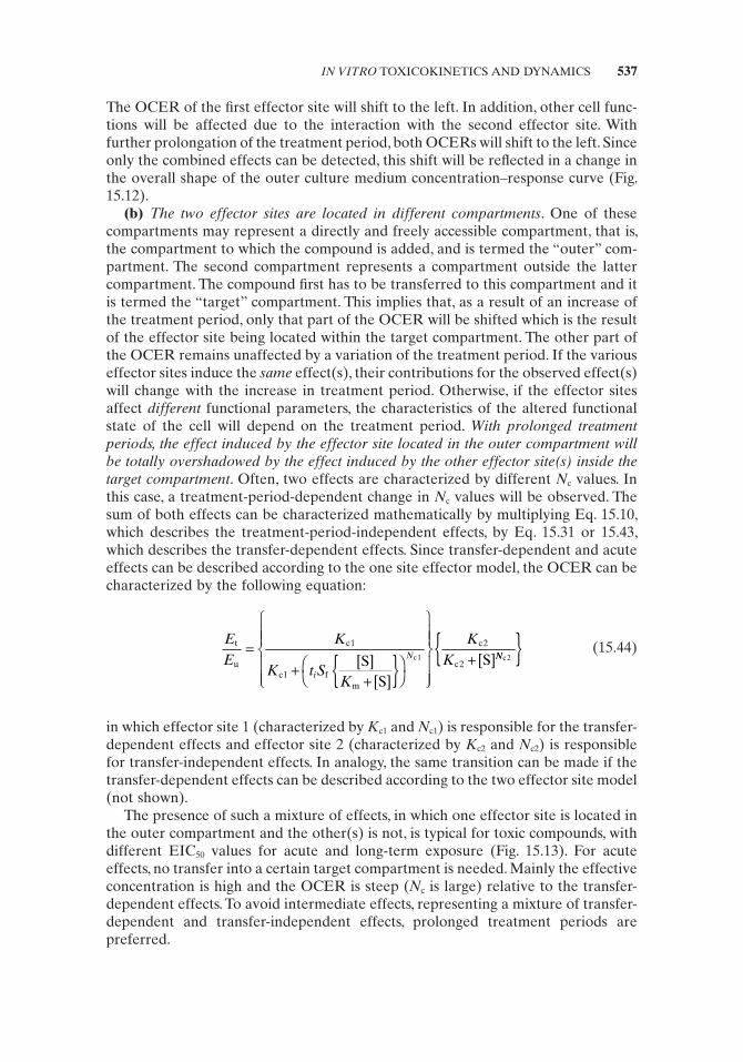
The presence of such a mixture of effects, in which one effector site is located in the outer compartment and the other(s) is not, is typical for toxic compounds, with different EIC 50 values for acute and long - term exposure (Fig. 15.13 ). For acute effects, no transfer into a certain target compartment is needed. Mainly the effective concentration is high and the OCER is steep ( N c is large) relative to the transfer - dependent effects. To avoid intermediate effects, representing a mixture of transfer - dependent and transfer - independent effects, prolonged treatment periods are preferred.
IN VITRO TOXICOKINETICS AND DYNAMICS 537
538 MODELING AND INTERPRETATION OF TOXICITY DATA
FIGURE 15.13 Simulation of an outer compartment compound concentration – effect rela-tionship (OCER) according to Eq. 15.44 in relation to the treatment period t i ( E u = 100). Target compartment effector site: N c1 = 1.5, K c1 = 0.1, S f = 10 and K m = 10. Outer compartment effector site: N c2 = 5, K c2 = 100,000; (all in arbitrary units).
–1 0 1
[Test compound] (log(concentration))
Activity (
% o
f co
ntr
ol)
100
80
60
40
20
0
ti=0.005
ti=0.15
ti=5
ti=0.5
Special Cases: The Accumulation Is Limited In some cases accumulation of the test compound in the target compartment seems to be limited. Apparently only during the fi rst part of the treatment period does a correlation between toxic effects and treatment period exist at a constant outer compartment test compound concentration.
An explanation for this phenomenon is the presence of a retro transport of the test compound (or its metabolite) out of the target compartment (Fig. 15.14 ). As a result, the accumulation in the target compartment is limited. The retrotransport may be due to diffusion or may be the result of a carrier - dependent retrotransport of the test compound. The increase of the target compartment concentration is maximum at small s i (Fig. 15.14 ). A maximum concentration is reached the moment that the outward fl ux is equivalent to the inward fl ux. It must be noted that test compounds that are metabolized or activated inside the target compartment and the metabolite or activated test compounds that are able to leave the target com-partment in one way or another behave identically.
The target compartment concentration s is dependent on the rat of infl ux (Fig. 15.14 left) or conversion rate (Fig. 15.14 right) and effl ux rate. This infl ux/conversion is constant due to a constant outer compartment concentration (Eq. 15.30 ). The effl ux, however, is dependent on the target compartment concentration and thus changes during the treatment period. If the effl ux is carrier dependent, this may be described, in analogy to Eq. 15.4 , as follows:
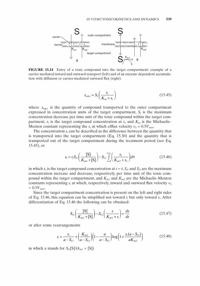
s S
sK s
ii
iout, f
m
=+
⎛⎝⎜
⎞⎠⎟
(15.45)
where s iout, is the quantity of compound transported to the outer compartment expressed in concentration units of the target compartment, S f is the maximum concentration decrease per time unit of the toxic compound within the target com-partment, s i is the target compound concentration at t i , and K m is the Michaelis – Menten constant representing the s i at which effl ux velocity v 0 = 0.5 V max .
The concentration s i can be described as the difference between the quantity that is transported into the target compartment (Eq. 15.30 ) and the quantity that is transported out of the target compartment during the treatment period (see Eq. 15.45 ), or
s t S
KS
sK s
di i
ti
=+
⎛⎝⎜
⎞⎠⎟ −
+⎛⎝⎜
⎞⎠⎟=
=
∫f1m
fm
SS
[ ][ ]1
220
τ
ττ
τ
τ
(15.46)
in which s τ is the target compound concentration at t = τ , S f1 and S f2 are the maximum concentration increase and decrease, respectively, per time unit of the toxic com-pound within the target compartment, and K m1 and K m2 are the Michaelis – Menten constants representing s i at which, respectively, inward and outward fl ux velocity v 0 = 0.5 V max .
Since the target compartment concentration is present on the left and right sides of Eq. 15.46 , this equation can be simplifi ed not toward t i but only toward s i . After differentiation of Eq. 15.46 the following can be obtained:
S
KS
sK s
dsdt
fm
fm
SS
11
22
[ ][ ]+
⎛⎝⎜
⎞⎠⎟ −
+⎛⎝⎜
⎞⎠⎟ =
(15.47)
or after some rearrangements
t
sa S
Ka S
aa S
s a SaK
ii i=
−+
−( ) −−( ) +
−( )f
m
f f
f
m2
2
2 2
2
2
1 1log( )
(15.48)
in which a stands for S f1 [S]/( k m1 + [S])
FIGURE 15.14 Entry of a toxic compound into the target compartment: example of a carrier mediated inward and outward transport (left) and of an enzyme - dependent accumula-tion with diffusion or carrier - mediated outward fl ux (right).
target compartment
outer compartmentS
s
Km1
carrier
barrier
Km2
S
sS
membrane
Km1
Km2
IN VITRO TOXICOKINETICS AND DYNAMICS 539
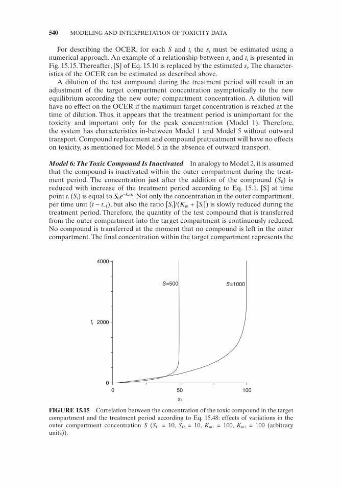
540 MODELING AND INTERPRETATION OF TOXICITY DATA
For describing the OCER, for each S and t i the s i must be estimated using a numerical approach. An example of a relationship between s i and t i is presented in Fig. 15.15 . Thereafter, [S] of Eq. 15.10 is replaced by the estimated s i . The character-istics of the OCER can be estimated as described above.
A dilution of the test compound during the treatment period will result in an adjustment of the target compartment concentration asymptotically to the new equilibrium according the new outer compartment concentration. A dilution will have no effect on the OCER if the maximum target concentration is reached at the time of dilution. Thus, it appears that the treatment period is unimportant for the toxicity and important only for the peak concentration ( Model 1 ). Therefore, the system has characteristics in - between Model 1 and Model 5 without outward transport. Compound replacement and compound pretreatment will have no effects on toxicity, as mentioned for Model 5 in the absence of outward transport.
Model 6: The Toxic Compound Is Inactivated In analogy to Model 2 , it is assumed that the compound is inactivated within the outer compartment during the treat-ment period. The concentration just after the addition of the compound ( S 0 ) is reduced with increase of the treatment period according to Eq. 15.1 . [S] at time point t i ( S i ) is equal to S e k ti
0− el . Not only the concentration in the outer compartment,
per time unit ( t − t − 1 ), but also the ratio [ S i ]/( K m + [ S i ]) is slowly reduced during the treatment period. Therefore, the quantity of the test compound that is transferred from the outer compartment into the target compartment is continuously reduced. No compound is transferred at the moment that no compound is left in the outer compartment. The fi nal concentration within the target compartment represents the
FIGURE 15.15 Correlation between the concentration of the toxic compound in the target compartment and the treatment period according to Eq. 15.48 : effects of variations in the outer compartment concentration S ( S f1 = 10, S f2 = 10, K m1 = 100, K m2 = 100 (arbitrary units)).
0 50 100
si
ti
4000
2000
0
S=500 S=1000
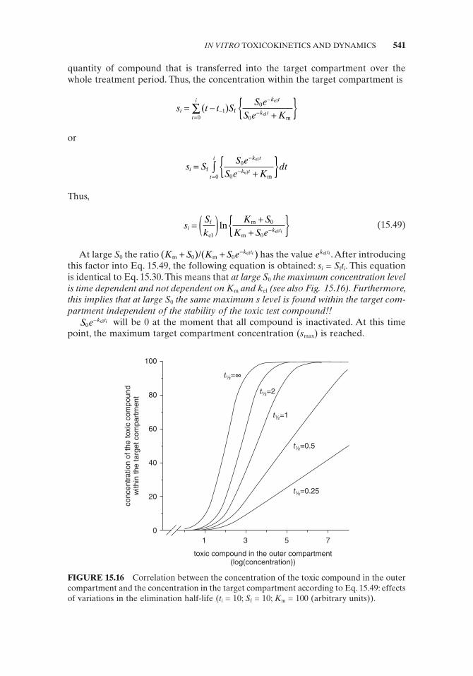
quantity of compound that is transferred into the target compartment over the whole treatment period. Thus, the concentration within the target compartment is
s t t S
S eS e K
i
k t
k tt
i
= −+{ }−
−
−=∑ ( )1
0
00f
m
el
el
or
s S
S eS e K
dti
k t
k tt
i
=+{ }−
−=∫f
m
el
el
0
00
Thus,
s
Sk
K SK S e
i k ti= ( ) +
+{ }−f
el
m
mel
ln 0
0 (15.49)
At large S 0 the ratio ( ) ( )K S K S e k tim m/ el+ + −
0 0 has the value ek tiel . After introducing this factor into Eq. 15.49 , the following equation is obtained: s i = S f t i . This equation is identical to Eq. 15.30 . This means that at large S 0 the maximum concentration level is time dependent and not dependent on K m and k el (see also Fig. 15.16 ). Furthermore, this implies that at large S 0 the same maximum s level is found within the target com-partment independent of the stability of the toxic test compound!!
S e k ti0
− el will be 0 at the moment that all compound is inactivated. At this time point, the maximum target compartment concentration ( s max ) is reached.
FIGURE 15.16 Correlation between the concentration of the toxic compound in the outer compartment and the concentration in the target compartment according to Eq. 15.49 : effects of variations in the elimination half - life ( t i = 10; S f = 10; K m = 100 (arbitrary units)).
1 3 5 7
toxic compound in the outer compartment(log(concentration))
concentr
ation o
f th
e toxic
com
pound
within
the targ
et co
mpart
ment
100
80
60
40
20
0
t½=0.25
t½=0.5
t½=1
t½=2
t½=∞
IN VITRO TOXICOKINETICS AND DYNAMICS 541
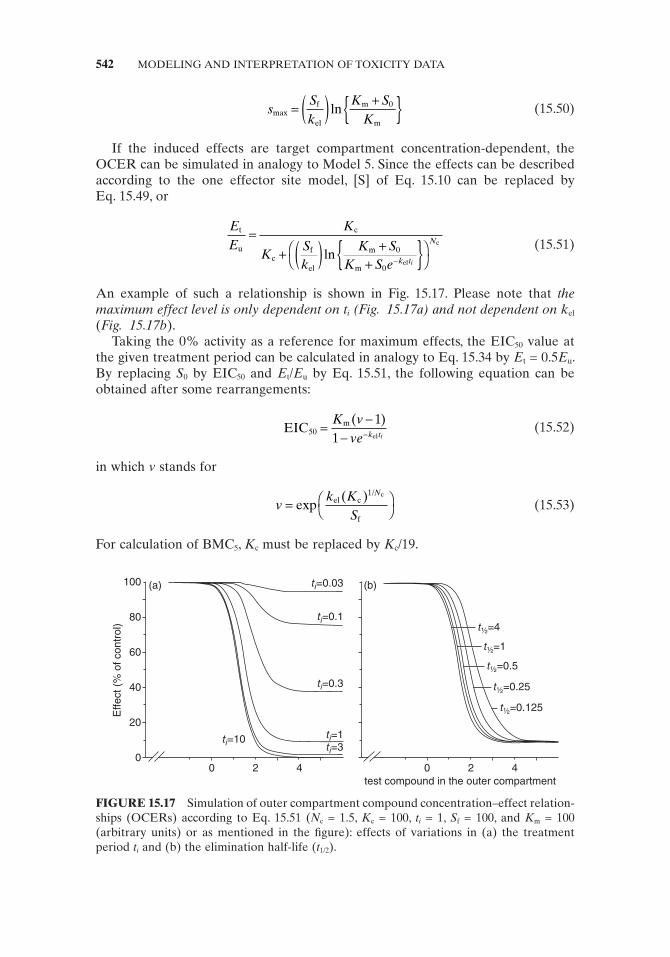
542 MODELING AND INTERPRETATION OF TOXICITY DATA
s
Sk
K SK
max ln= ( ) +{ }f
el
m
m
0
(15.50)
If the induced effects are target compartment concentration - dependent, the OCER can be simulated in analogy to Model 5 . Since the effects can be described according to the one effector site model, [S] of Eq. 15.10 can be replaced by Eq. 15.49 , or
EE
K
KSk
K SK S e k t
N
i
t
u
c
cf
el
m
mel
c=
+ ( ) ++{ }⎛
⎝⎞⎠−ln 0
0
(15.51)
An example of such a relationship is shown in Fig. 15.17 . Please note that the maximum effect level is only dependent on t i (Fig. 15.17a ) and not dependent on k el ( Fig. 15.17b ).
Taking the 0% activity as a reference for maximum effects, the EIC 50 value at the given treatment period can be calculated in analogy to Eq. 15.34 by E t = 0.5 E u . By replacing S 0 by EIC 50 and E t / E u by Eq. 15.51 , the following equation can be obtained after some rearrangements:
EIC m
el50
11
=−
− −
K vve k ti
( )
(15.52)
in which v stands for
v
k KS
N
= ⎛⎝
⎞⎠exp
( )el c/
f
c1
(15.53)
For calculation of BMC 5 , K c must be replaced by K c /19.
FIGURE 15.17 Simulation of outer compartment compound concentration – effect relation-ships (OCERs) according to Eq. 15.51 ( N c = 1.5, K c = 100, t i = 1, S f = 100, and K m = 100 (arbitrary units) or as mentioned in the fi gure): effects of variations in (a) the treatment period t i and (b) the elimination half - life ( t 1/2 ).
100 (a) (b)
80
60
40
20
00 2 4 0 2
test compound in the outer compartment
Eff
ect
(% o
f co
ntr
ol)
4
ti=0.03
ti=0.1t½=4
t½=1
t½=0.5
t½=0.25
t½=0.125
ti=0.3
ti=10 ti=1ti=3
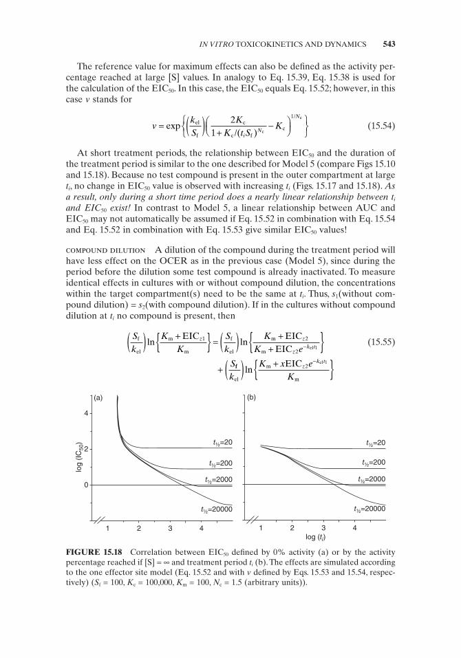
The reference value for maximum effects can also be defi ned as the activity per-centage reached at large [S] values. In analogy to Eq. 15.39 , Eq. 15.38 is used for the calculation of the EIC 50 . In this case, the EIC 50 equals Eq. 15.52 ; however, in this case v stands for
v
kS
KK t S
Ki
N
N
= ( ) +−⎛
⎝⎜⎞⎠⎟
⎧⎨⎩
⎫⎬⎭
exp( )
el
f
c
c fc
/
/ c
c21
1
(15.54)
At short treatment periods, the relationship between EIC 50 and the duration of the treatment period is similar to the one described for Model 5 (compare Figs 15.10 and 15.18 ). Because no test compound is present in the outer compartment at large t i , no change in EIC 50 value is observed with increasing t i (Figs. 15.17 and 15.18 ). As a result, only during a short time period does a nearly linear relationship between t i and EIC 50 exist! In contrast to Model 5 , a linear relationship between AUC and EIC 50 may not automatically be assumed if Eq. 15.52 in combination with Eq. 15.54 and Eq. 15.52 in combination with Eq. 15.53 give similar EIC 50 values!
compound dilution A dilution of the compound during the treatment period will have less effect on the OCER as in the previous case ( Model 5 ), since during the period before the dilution some test compound is already inactivated. To measure identical effects in cultures with or without compound dilution, the concentrations within the target compartment(s) need to be the same at t i . Thus, s 1 (without com-pound dilution) = s 2 (with compound dilution). If in the cultures without compound dilution at t i no compound is present, then
Sk
KK
Sk
KK e
S
z z
zk t
f
el
m
m
f
el
m
m
EIC EICEIC el( ) +{ } = ( ) +
+{ }+
−ln ln1 2
21
ff
el
m
m
EIC el
kK x e
Kz
k t( ) +{ }−
ln 21
(15.55)
FIGURE 15.18 Correlation between EIC 50 defi ned by 0% activity (a) or by the activity percentage reached if [S] = ∞ and treatment period t i (b). The effects are simulated according to the one effector site model (Eq. 15.52 and with v defi ned by Eqs. 15.53 and 15.54 , respec-tively) ( S f = 100, K c = 100,000, K m = 100, N c = 1.5 (arbitrary units)).
(a)
1 32 4
t½=20
t½=200
t½=2000
t½=20000
t½=20
t½=200
t½=2000
t½=20000
4
2
0
(b)
1 32
log (ti)
log (
IC50)
4
IN VITRO TOXICOKINETICS AND DYNAMICS 543

544 MODELING AND INTERPRETATION OF TOXICITY DATA
in which EIC z 1 is the obtained EIC z in experiments without dilution, EIC z 2 is the EIC z in experiments in which the compound was diluted during the treatment period, ( S f / k el )ln{( k m + EIC z 1 )/ k m } is the test compound concentration in the target compartment at t i in experiments without dilution according to Eq. 15.48 , ( ) ln{( )}S k K K ez z
k tf el m m/ EIC )/( EIC el+ + −
2 21 is the test compound
concentration in the target compartment at t 1 according to Eq. 15.47 , and ( ) ln{( }S k K x e Kz
k tf el m m/ EIC )/el+ −
21 is the increase of target compartment concentra-
tion after dilution by a factor x over the period t 1 to t i (according to Eq. 15.50 ). After a rearrangement of Eq. 15.55 , we fi nd
k
tK
K x xz z
z z zel
m
m
EIC EICEIC EIC EIC
=−( ) −
− + −⎛⎝⎜
⎞111
2 1
2 1 2
ln( )
{ ( ) }⎠⎠⎟
(15.56)
or
K
x ex e
z z zk t
zk t
z zm
EIC EIC EICEIC EIC EIC
el
el=
−− + −
−
−
( )( )
2 1 2
2 1 2
1
11 (15.57)
The same equations can also be used if experiments with different treatment periods are compared. In this case, x = 0 and t 1 and t i represent the different treat-ment periods. The disadvantage of Eq. 15.56 and 15.57 is that K m has to be known in order to calculate k el . It may be possible to estimate k el and K m by including within the same experiment the effects of a dilution at different time points to obtain Eq. 15.57 with other values for EIC z 2 and t 1 . Since in both obtained equations the value for K m is the same, k el can theoretically be resolved.
A more complex situation exists if at the end of the treatment period not all test compound is inactivated. In this case, a correction needs to be included for the remaining compound. Therefore, Eq. 15.50 may not be used. Under the present assumptions, Eq. 15.55 is adapted to
Sk
KK e
Sk
KK
z
zk t
z
i
f
el
m
m
f
el
m
m
EICEIC
EICEICel( ) +
+{ } = ( ) ++−ln ln1
1
2
zzk t
zk t
zk t k
e
Sk
K x eK x e e
i
2
2
2
1
1
−
−
− −
{ }+ ( ) +
+
el
el
el e
f
el
m
m
EICEIC
lnll ( )t ti−{ }1
or after rearrangement,
K x e xz zk t t
z z z
z
im EIC EIC EIC EIC EIC
EIC
el= − + − +− −{( ) ( )
(
( )1 1 2 2 1 2
2
1
−−− + −
− −
−
EIC EIC /
EIC EIC EIC
el
el
z zk t t
z z zk
e
x x e
i1 2
2 2 1
1
1
) }
{( ) ( )
( )
(( ) }t ti− 1
(15.58)
Again, by changing the time point of dilution as mentioned before, k el and K m can theoretically be calculated.
compound replacement Compound replacement during treatment maximally results in a doubling of the target compartment concentration if all compound is inactivated at the moment of replacement and in addition at the moment that the
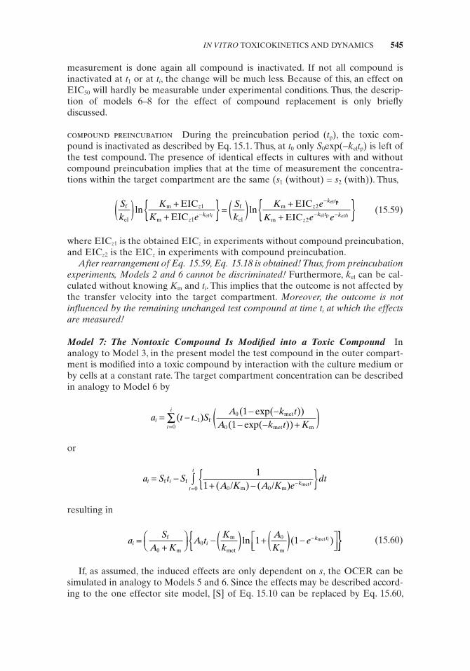
measurement is done again all compound is inactivated. If not all compound is inactivated at t 1 or at t i , the change will be much less. Because of this, an effect on EIC 50 will hardly be measurable under experimental conditions. Thus, the descrip-tion of models 6 – 8 for the effect of compound replacement is only briefl y discussed.
compound preincubation During the preincubation period ( t p ), the toxic com-pound is inactivated as described by Eq. 15.1 . Thus, at t 0 only S 0 exp( − k el t p ) is left of the test compound. The presence of identical effects in cultures with and without compound preincubation implies that at the time of measurement the concentra-tions within the target compartment are the same ( s 1 (without) = s 2 (with)). Thus,
Sk
KK e
Sk
K ez
zk t
zk t
i
f
el
m
m
f
el
mEICEIC
EICel
el( ) ++{ } = ( ) +
−
−
ln ln1
1
2pp
el p elm EICK e ez
k t k ti+{ }− −2
(15.59)
where EIC z 1 is the obtained EIC z in experiments without compound preincubation, and EIC z 2 is the EIC z in experiments with compound preincubation.
After rearrangement of Eq. 15.59 , Eq. 15.18 is obtained! Thus, from preincubation experiments, Models 2 and 6 cannot be discriminated! Furthermore, k el can be cal-culated without knowing K m and t i . This implies that the outcome is not affected by the transfer velocity into the target compartment. Moreover, the outcome is not infl uenced by the remaining unchanged test compound at time t i at which the effects are measured!
Model 7: The Nontoxic Compound Is Modifi ed into a Toxic Compound In analogy to Model 3 , in the present model the test compound in the outer compart-ment is modifi ed into a toxic compound by interaction with the culture medium or by cells at a constant rate. The target compartment concentration can be described in analogy to Model 6 by
a t t S
A k tA k t K
it
i
= −− −
− − +( )−=∑ ( )
( exp( ))( exp( ))
10
00
11
fmet
met m
or
a S t S
A K A K edti i k t
t
i
= −+ −{ }−
=∫f f
m m/ / met
11 0 00 ( ) ( )
resulting in
a
SA K
A tKk
AK
ei ik ti=
+⎛⎝⎜
⎞⎠⎟ − ( ) + ( ) −⎡
⎣⎢⎤⎦⎥{ −f
m
m
met m
met
00
01 1ln ( ) }}
(15.60)
If, as assumed, the induced effects are only dependent on s , the OCER can be simulated in analogy to Models 5 and 6 . Since the effects may be described accord-ing to the one effector site model, [S] of Eq. 15.10 can be replaced by Eq. 15.60 ,
IN VITRO TOXICOKINETICS AND DYNAMICS 545

546 MODELING AND INTERPRETATION OF TOXICITY DATA
or
EE
K
KS
A KA t
Kk
AK
eik ti
t
u
c
cf
m
m
met m
met
=+
+( ) − ( ) + ( ) −{ }{ }−
00
01 1ln ( )⎛⎛⎝
⎞⎠
Nc
(15.61)
Since the transfer from the outer compartment into the target compartment (or the enzymatic modifi cation of S to s * ; see Fig. 15.7 ) is a rate - limiting process, only at low concentrations does the rate of transfer parallel the outer compartment concentration of the toxic product (Fig. 15.19 ). At large concentrations, this transfer is constant and is not or only negligibly changed by an increase in the outer com-partment concentration. If the treatment period is increased, a disproportionate increase in target compartment concentration is seen if the t 1/2 value relative to the treatment period is large (slow activation; Fig. 15.20 ). Under testing conditions, the shift in OCER of the toxic product is larger than expected if erroneously Model 5 is assumed. Thus a compound dilution affects the EIC z value more, as expected if we assume Model 5 . At small t 1/2 values, no difference between the present model and Model 5 can be detected in dilution and preincubation experiments under experimental conditions. The equations describing the effects of compound dilution, compound replacement, and compound preincubation are extremely complex. Since a suspicion of compound activation implies retesting with the toxic product, a more detailed description is not needed. However, if under some circumstances such a description is necessary, the equations can easily be derived from Eq. 15.60 .
Model 8: The Nontoxic Test Compound Is Transformed into a Toxic Product that Afterwards Is Inactivated For the sake of completeness, Model 8 is mentioned in
FIGURE 15.19 Correlation between the concentration of the toxic compound in the outer compartment and the concentration in the target compartment according to Eq. 15.60 : effects of variations in the elimination half - life ( t i = 10; S f = 10; K m = 100 (arbitrary units)).
(a)
1 3 5
t½=0.2
t½=2
t½=20
t½=200
t½=2000
100
80
60
40
20
0
concentr
ation o
f th
e toxic
meta
bolit
e
within
the targ
et com
part
ment
test compound in the outer compartment
(log (concentration))
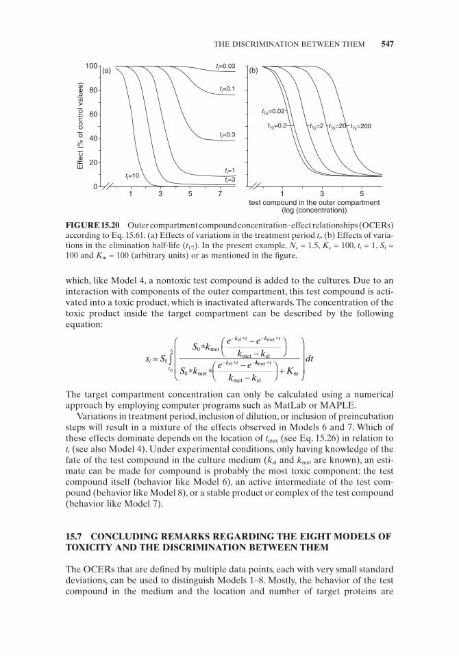
which, like Model 4 , a nontoxic test compound is added to the cultures. Due to an interaction with components of the outer compartment, this test compound is acti-vated into a toxic product, which is inactivated afterwards. The concentration of the toxic product inside the target compartment can be described by the following equation:
s SS k
e ek k
S ke ei
k t k t
k t=∗ −
−⎛⎝
⎞⎠
∗ ∗ −
− ∗ − ∗
− ∗ −f
metmet el
met
el met
el
0
0
kk tt
t
k kK
dti
met
met elm
∗
−⎛⎝
⎞⎠ +
⎛
⎝
⎜⎜⎜
⎞
⎠
⎟⎟⎟
∫0
The target compartment concentration can only be calculated using a numerical approach by employing computer programs such as MatLab or MAPLE.
Variations in treatment period, inclusion of dilution, or inclusion of preincubation steps will result in a mixture of the effects observed in Models 6 and 7 . Which of these effects dominate depends on the location of t max (see Eq. 15.26 ) in relation to t i (see also Model 4 ). Under experimental conditions, only having knowledge of the fate of the test compound in the culture medium ( k el and k met are known), an esti-mate can be made for compound is probably the most toxic component: the test compound itself (behavior like Model 6 ), an active intermediate of the test com-pound (behavior like Model 8 ), or a stable product or complex of the test compound (behavior like Model 7 ).
15.7 CONCLUDING REMARKS REGARDING THE EIGHT MODELS OF TOXICITY AND THE DISCRIMINATION BETWEEN THEM
The OCERs that are defi ned by multiple data points, each with very small standard deviations, can be used to distinguish Models 1 – 8 . Mostly, the behavior of the test compound in the medium and the location and number of target proteins are
FIGURE 15.20 Outer compartment compound concentration – effect relationships (OCERs) according to Eq. 15.61 . (a) Effects of variations in the treatment period t i . (b) Effects of varia-tions in the elimination half - life ( t 1/2 ). In the present example, N c = 1.5, K c = 100, t i = 1, S f = 100 and K m = 100 (arbitrary units) or as mentioned in the fi gure.
(a) (b)
1 53 7
ti=0.03
ti=0.1
ti=0.3
ti=1ti=10
ti=3
100
80
60
40
20
01 3 5
Effect (%
of contr
ol valu
es)
test compound in the outer compartment(log (concentration))
t½=0.02
t½=0.2 t½=2 t½=20 t½=200
THE DISCRIMINATION BETWEEN THEM 547
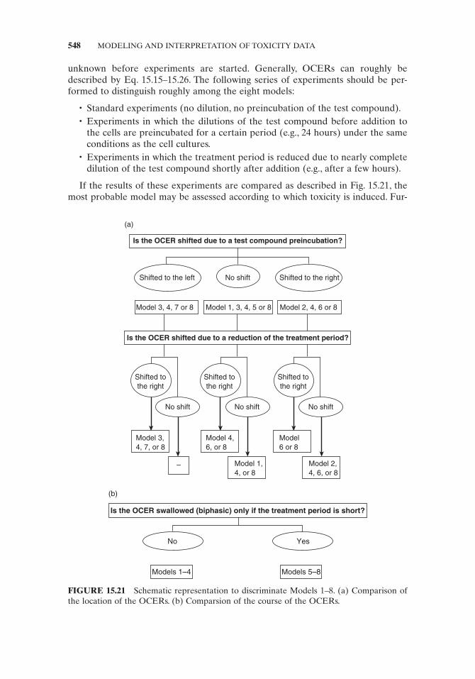
548 MODELING AND INTERPRETATION OF TOXICITY DATA
unknown before experiments are started. Generally, OCERs can roughly be described by Eq. 15.15 – 15.26. The following series of experiments should be per-formed to distinguish roughly among the eight models:
• Standard experiments (no dilution, no preincubation of the test compound). • Experiments in which the dilutions of the test compound before addition to
the cells are preincubated for a certain period (e.g., 24 hours) under the same conditions as the cell cultures.
• Experiments in which the treatment period is reduced due to nearly complete dilution of the test compound shortly after addition (e.g., after a few hours).
If the results of these experiments are compared as described in Fig. 15.21 , the most probable model may be assessed according to which toxicity is induced. Fur-
FIGURE 15.21 Schematic representation to discriminate Models 1 – 8 . (a) Comparison of the location of the OCERs. (b) Comparsion of the course of the OCERs.
Is the OCER shifted due to a test compound preincubation?
Is the OCER shifted due to a reduction of the treatment period?
Shifted to the left
(a)
No shift Shifted to the right
Model 3, 4, 7 or 8 Model 1, 3, 4, 5 or 8 Model 2, 4, 6 or 8
Shifted to
the right
No shift No shift No shift
Shifted to
the right
Shifted to
the right
Model 3,
4, 7, or 8
Model 4,
6, or 8
Model 1,
4, or 8
Model 2,
4, 6, or 8
Model
6 or 8
–
Is the OCER swallowed (biphasic) only if the treatment period is short?
No
(b)
Models 1–4 Models 5–8
Yes
thermore, the data may help to decide which further experiments, like measurement of the test compound concentration and/or its metabolite(s) at the end of the treat-ment period, are needed to further specify the obtained characteristics.
In summary, the present chapter describes tools to elucidate the toxicomecha-nisms under in vitro conditions. For this, equations were developed to describe in vitro toxicokinetics and toxicodynamics under various conditions and assumptions.
ACKNOWLEDGMENT
The present study was supported by the European Commission through the specifi c targeted research project CellForce (Contract No. NMP4 - CT - 2005 - 016626).
REFERENCES
1. Dost FH . Grundlagen der Pharmakokinetik . Stuttgart : Thieme ; 1968 , p 450 . 2. Hill AV . The possible effects of the aggregation of the molecules of haemoglobin on its
oxygen dissociation curve . J Physiol (London) 1913 ; 40 : IV – VII . 3. Bruinink A . Serum - free monolayer cultures of fetal chick brain and retina: immunoassays
of developmental markers, mathematical data analysis, and establishment of optimal culture conditions . In Zbinden G , Ed. The Brain in Bits and Pieces . Zollikon : MTC Verlag ; 1992 , pp 23 – 50 .
4. Filipsson AF , Sand S , Nilsson J , Victorin K . The benchmark dose method — review of available models, and recommendations for application in health risk assessment . Crit Rev Toxicol 2003 ; 33 : 505 – 542 .
5. Auton TR . Calculation of benchmark doses from teratology data . Regul Toxicol Pharma-col 1994 ; 19 : 152 – 167 .
6. Links JM , Schwartz BS , Simon D , Bandeen - Roche K , Stewart WF . Characterization of toxicokinetics and toxicodynamics with linear systems theory: application to lead - associ-ated cognitive decline . Environ Health Perspect 2001 ; 109 : 361 – 368 .
7. Nakayama Y , Kishida F , Nakatsuka I , Matsuo M . Simulation of the toxicokinetics of trichloroethylene, methylene chloride, styrene and n - hexane by a toxicokinetics/toxico-dynamics model using experimental data . Environ Sci 2005 ; 12 : 21 – 32 .
8. Bois FY , Gelman A , Jiang J , Maszle DR , Zeise L , Alexeef G . Population toxicokinetics of tetrachloroethylene . Arch Toxicol 1996 ; 70 : 347 – 355 .
9. Haddad S , Krishnan K . Physiological modeling of toxicokinetic interactions: implications for mixture risk assessment . Environ Health Perspect 1998 ; 106 ( Suppl 6 ): 1377 – 1384 .
10. Bruinink A , Rasonyi T , Sidler C . Reduction of ochratoxin A toxicity by heat - induced epimerization. In vitro effects of ochratoxins on embryonic chick meningeal and other cell cultures . Toxicology 1997 ; 118 : 205 – 210 .
11. Bruinink A , Sidler C . The neurotoxic effects of ochratoxin - A are reduced by protein binding but are not affected by l - phenylalanine . Toxicol Appl Pharmacol 1997 ; 146 : 173 – 179 .
12. Bruinink A , Rasonyi T , Sidler C . Differences in neurotoxic effects of ochratoxin A, ochra-cin and ochratoxin - alpha in vitro . Natural Toxins 1998 ; 6 : 173 – 177 .
13. Bruinink A , Faller P , Sidler C , Bogumil R , Vasak M . Growth inhibitory factor and zinc affect neural cell cultures in a tissue specifi c manner . Chemi - Biol Interact 1998 ; 115 : 167 – 174 .
REFERENCES 549
550 MODELING AND INTERPRETATION OF TOXICITY DATA
14. M ü ller JP , Bruinink A . Neurotoxic effects of aluminium on embryonic chick brain cul-tures . Acta Neuropathol 1994 ; 88 : 359 – 366 .
15. Bruinink A , Birchler F . Effects of cisplatin and ORG.2766 in chick embryonic brain cell cultures . Arch Toxicol 1993 ; 67 : 325 – 329 .
16. Bruinink A , Reiser P , M ü ller M , G ä hwiler BH , Zbinden G . Neurotoxic effects of bismuth in vitro . Toxicol In Vitro 1992 ; 6 : 285 – 293 .
17. Bruinink A , Zimmermann G , Riesen F . Neurotoxic effects of chloroquine in vitro . Arch Toxicol 1991 ; 65 : 480 – 484 .
18. Bruinink A , Sidler C , Birchler F . Neurotrophic effects of transferrin on embryonic chick brain and neural retina cell cultures . Int J Dev Neurosci 1996 ; 14 : 785 – 795 .
19. Goldoni M , Vettori MV , Alinovi R , Caglieri A , Ceccatelli S , Mutti A . Models of neuro-toxicity: extrapolation of benchmark doses in vitro . Risk Anal 2003 ; 23 : 505 – 514 .
20. Progress Report of the Ecological Committee on FIFRA Risk Assessment Methods: V . Terrestrial Effects Assessment . US EPA; 2005 .
21. Stephens DN , Voet B . Differential effects of anxiolytic and non - anxiolytic benzodiazepine receptor ligands on performance of a differential reinforcement of low rate (DRL) schedule . Behav Pharmacol 1994 ; 5 : 4 – 14 .
22. Michaelis L , Menten ML . Die Kinetik der Invertinwirkung . Biochem Z 1913 ; 49 : 333 – 369 .