precipitationmodule(tc-prisma)userguide … · contents introductiontotheprecipitation...

Precipitation Module (TC-PRISMA) User GuideVersion 2016b

Copyright 2016 Thermo-Calc Software AB. Allrights reserved.

Information in this document is subject to changewithout notice. The software described in thisdocument is furnished under a license agreementor nondisclosure agreement. The softwaremay beused or copied only in accordance with the termsof those agreements.

Thermo-Calc Software AB or Thermo-CalcSoftware, Inc..

Norra Stationsgatan 93, SE-113 64 Stockholm,Sweden

+46 8 545 959 30

[email protected]

www.thermocalc.com

2 of 2

Contents

Introduction to the PrecipitationModule (TC-PRISMA) 3

About the Precipitation Module (TC-PRISMA) 4

Help Resources 5

Online and Context Help 5

Precipitation Module (TC-PRISMA) Options 7

Precipitation Simulation Template 7

Precipitation Calculator 8

Demo Database Packages for theExamples Collection 8

Demonstration (Demo) Mode 9

Selecting the Disordered Phase as a MatrixPhase 9

Precipitation Module Examples 10

Example 13: Isothermal Precipitationof Al3Sc 10

Plot Results 12

Example 14: Stable and MetastableCarbides - Isothermal 12

Plot Results 13

Example 15: Stable and MetastableCarbides - TTT Diagram 14

Plot Results 15

Example 16: Precipitation of Iron Car-bon Cementite 15

Volume Fraction 16

Example 17: Precipitation of g’ in NiSuperalloys - Isothermal 17

Volume Fraction 18

Number Density 18

Mean Radius 19

Example 18: Precipitation of g’ in NiSuperalloys - Non-isothermal 19

Mean Radius Ni-8Al-8Cr 21

Mean Radius Ni-10Al-10CR 21

Size Distribution (PSD) Ni-8Al-8Cr 22

Size Distribution (PSD) Ni-10Al-10Cr 22

Using the Precipitation Calculator 23


Configuration Window 24

Conditions Tab Settings 24

Isothermal 26

Non-Isothermal 26

TTT-Diagram 27

Options Tab Settings 27

Growth RateModel 27

Numerical Parameters 27

Plot Renderer for the Precipitation Cal-culator 28

Points 29

Time 29

Excess Kurtosis 30

Minimum Separation Limit (ValleyDepth Ratio) 30

Minimum Peak 30

Theoretical Models 31

1 of 53

Theory Overview 32

Integration of the Precipitation Mod-ule into Thermo-Calc 33

Nucleation Theory 33

Homogeneous Nucleation 33

Heterogeneous Nucleation 37

Non-Spherical Particles and the EffectofWetting Angle 37

Shape Factors 38

Critical Radius and Activation Energy 39

Other Parameters 40

Zeldovitch Factor 40

Impingement Rate 41

Nucleation Site Density 41

Growth Rate 41

Output 41

The Shape and Size of Grains in theMatrix 42

Nucleation During a Non-isothermal Pro-cess 43

Growth 44

Coarsening 46

Continuity Equation 47

Mass Conservation 47

Numerical Method 48

Maximum time step fraction 48

Number of grid points over one orderofmagnitude in r 48

Maximum number of grid points over 49

one order ofmagnitude in r

Minimum number of grid points overone order ofmagnitude in r 49

Maximum relative radius change 49

Maximum relative volume fraction ofsubcritical particles allowed to dissolvein one time step 49

Relative radius change for avoidingclass collision 50

Maximum overall volume change 50

Maximum relative change of nuc-leation rate in logarithmic scale 50

Maximum relative change of criticalradius 50

Minimum radius for a nucleus to beconsidered as a particle 50

Maximum time step during heatingstages 51

Numerical Control Parameters DefaultValues 51

Interfacial Energy 51

Estimation of Coherent InterfacialEnergy 51

Precipitation Module (TC-PRISMA) References 52

2 of 53

Precipitation Module (TC-PRISMA) User Guide

Introduction to the Precipitation Module (TC-PRISMA) ǀ 3 of 53

Introduction to the Precipitation Module (TC-PRISMA)In this section:

About the Precipitation Module (TC-PRISMA) 4

Help Resources 5

Precipitation Module (TC-PRISMA) Options 7

Selecting the Disordered Phase as a Matrix Phase 9

Precipitation Module Examples 10


About the Precipitation Module (TC-PRISMA) ǀ 4 of 53

About the Precipitation Module (TC-PRISMA)

As of Thermo-Calc version 2016a, TC-PRISMA is no longer a standalone program. It isintegrated into the Thermo-Calc Graphical Mode and considered an add-on module calledthe Precipitation Module. It is also available for all platforms (Windows, Mac and Linux). Ifyou have older versions of the TC-PRISMA software that you want to uninstall, follow theinstructions to remove this program component as described in the Thermo-CalcInstallation Guide.

The Precipitation Module, previously only referred to as TC-PRISMA, is an add-on module to the coreThermo-Calc software. The Precipitation Module itself is a general computational tool for simulatingkinetics of diffusion controlled multi-particle precipitation processes in multicomponent and multi-phasealloy systems.

Precipitation, formation of particles of a second phase, or second phases from a supersaturated solidsolution matrix phase, is a solid state phase transformation process that has been exploited to improvethe strength and toughness of various structural alloys for many years. This process is thermochemicallydriven and fully governed by system (bulk and interface) thermodynamics and kinetics.

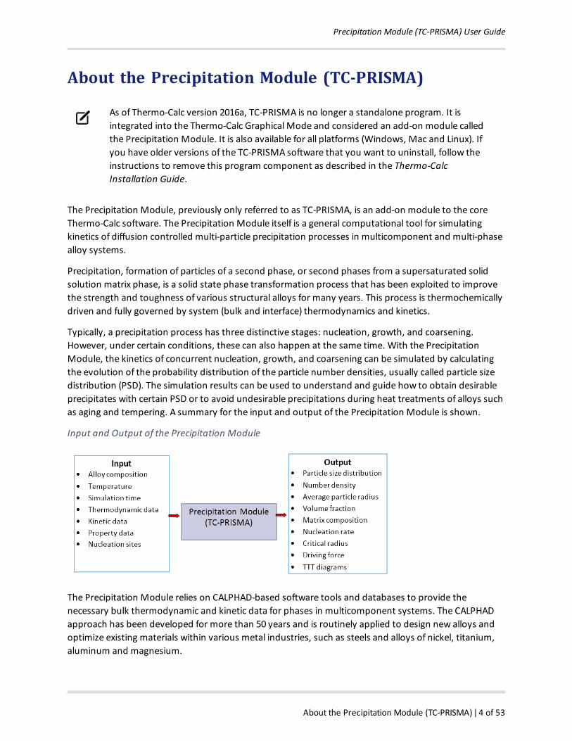
Typically, a precipitation process has three distinctive stages: nucleation, growth, and coarsening.However, under certain conditions, these can also happen at the same time. With the PrecipitationModule, the kinetics of concurrent nucleation, growth, and coarsening can be simulated by calculatingthe evolution of the probability distribution of the particle number densities, usually called particle sizedistribution (PSD). The simulation results can be used to understand and guide how to obtain desirableprecipitates with certain PSD or to avoid undesirable precipitations during heat treatments of alloys suchas aging and tempering. A summary for the input and output of the Precipitation Module is shown.

Input and Output of the Precipitation Module

The Precipitation Module relies on CALPHAD-based software tools and databases to provide thenecessary bulk thermodynamic and kinetic data for phases in multicomponent systems. The CALPHADapproach has been developed for more than 50 years and is routinely applied to design new alloys andoptimize existing materials within various metal industries, such as steels and alloys of nickel, titanium,aluminum and magnesium.


Help Resources ǀ 5 of 53

The power of this approach is due to the adopted methodology where free energy and atomic mobilityof each phase in a multicomponent system can bemodeled hierarchically from lower order systems, andmodel parameters are evaluated in a consistent way by considering both experimental data and ab-initiocalculation results. The Precipitation Module is directly integrated into Thermo-Calc, a CALPHAD-basedcomputer program for calculating phase equilibrium. Another add-on module, the Diffusion Module(DICTRA) is available for diffusion controlled phase transformation in multicomponent systems.

With Thermo-Calc and the accompanying thermodynamic and mobility databases, almost allfundamental phase equilibrium and phase transformation information can be calculated withoutunnecessary and inaccurate approximations. For example you can calculate:

l Driving forces for nucleation and growth

l Operating tie-lines under local equilibrium conditions

l Deviations from local equilibrium at interfaces due to interface friction

l Atomic mobilities or diffusivities in the matrix phase

In addition to bulk thermodynamic and kinetic data, a few other physical properties, such as interfacialenergy and volume, are needed in precipitation models. These additional physical parameters can beobtained by experiments or other estimation models or first principles calculations. Volume data forsteels and nickel-based alloys have already been assessed and included in TCFE, TCNI, and TCALdatabases. The Precipitation Module has an estimation model available for interfacial energy.

This guide is a supplement to the full Thermo-Calc documentation set. It is recommendedthat you use the Online Help from within Thermo-Calc or the PDF called PrecipitationModule (TC-PRISMA) Documentation Set to navigate all the content. SeeHelp Resourcesbelow to learn how to access this information if you have not already done so.

Help ResourcesOnline and Context HelpOnline Help

To access online help in a browser, open Thermo-Calc and select Help →Online Help. The content opensin a browser but uses local content so you don't need an internet connection.

Context Help

When you are in Graphical Mode, you can access feature help (also called topic-sensitive or context help)for the activity nodes in the tree.

1. In the Project window, click a node. For example, System Definer.

2. In the lower left corner of the Configuration window, click the help button .


Online and Context Help ǀ 6 of 53

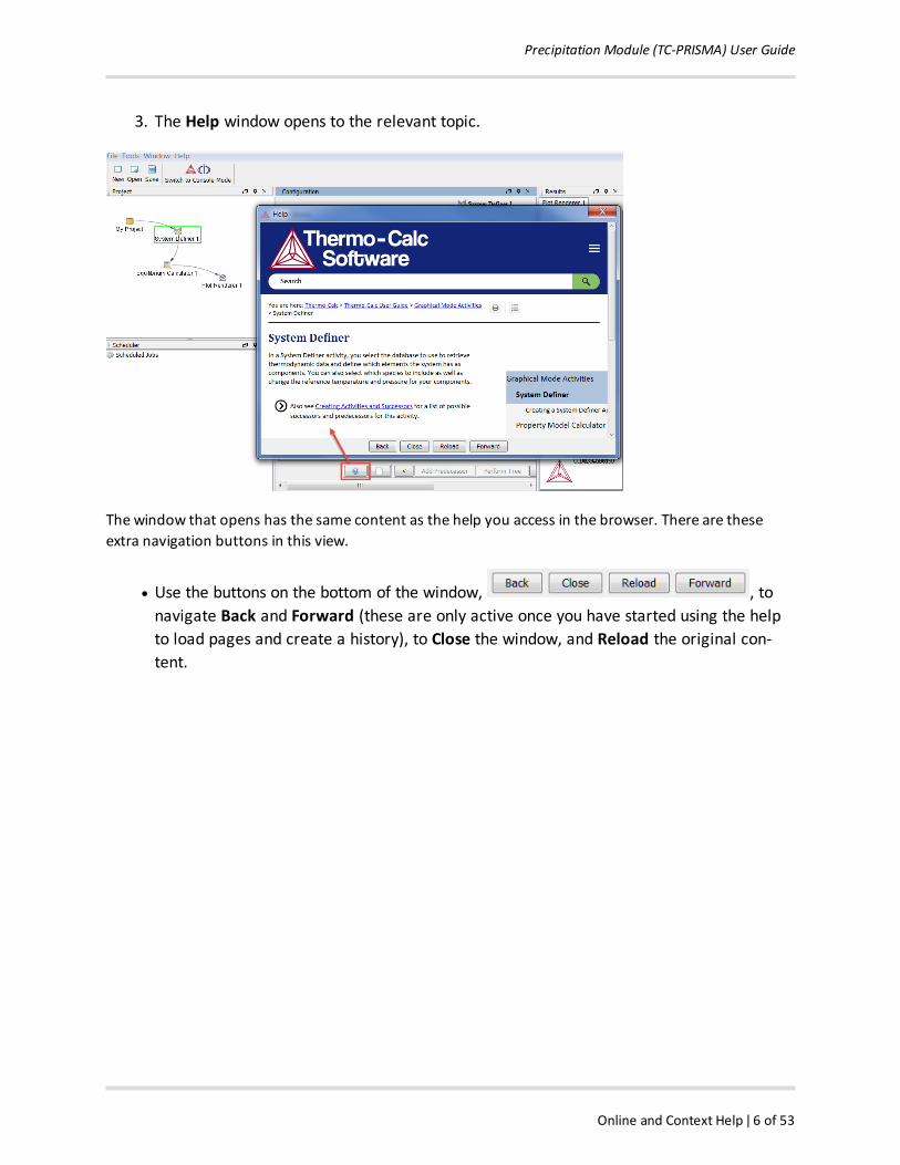
3. The Help window opens to the relevant topic.

The window that opens has the same content as the help you access in the browser. There are theseextra navigation buttons in this view.

l Use the buttons on the bottom of the window, , tonavigate Back and Forward (these are only active once you have started using the helpto load pages and create a history), to Close the window, and Reload the original con-tent.


Precipitation Module (TC-PRISMA) Options ǀ 7 of 53

Console Mode Help

ConsoleMode is for Thermo-Calc and the Diffusion Module (DICTRA).

In ConsoleMode at the command line prompt, you can access help in these ways:

l For a list of all the available commands in the current module, at the prompt type aquestion mark (?) and press <Enter>.

l For a description of a specific command, type Help followed by the name of the com-mand. You can only get online help about a command related to the current module youare in.

l For general system information type Information. Specify the subject or type ? and theavailable subjects are listed. This subject list is specific to the current module.

Precipitation Module (TC-PRISMA) OptionsThe Precipitation Module, previously only referred to as TC-PRISMA, is an add-on module to the coreThermo-Calc software. A separate license is required to perform calculations for more than twocomponents. Without it you are able to use themodule in Demo Mode. SeeDemonstration(Demo) Mode on page 9 to learn more.

Precipitation Simulation TemplateA Precipitation Simulation template is available to all Thermo-Calc users.

If you are using the Precipitation Module in Demo Mode, seeDemonstration (Demo) Modeon page 9 for what is available to you.

Using the Template

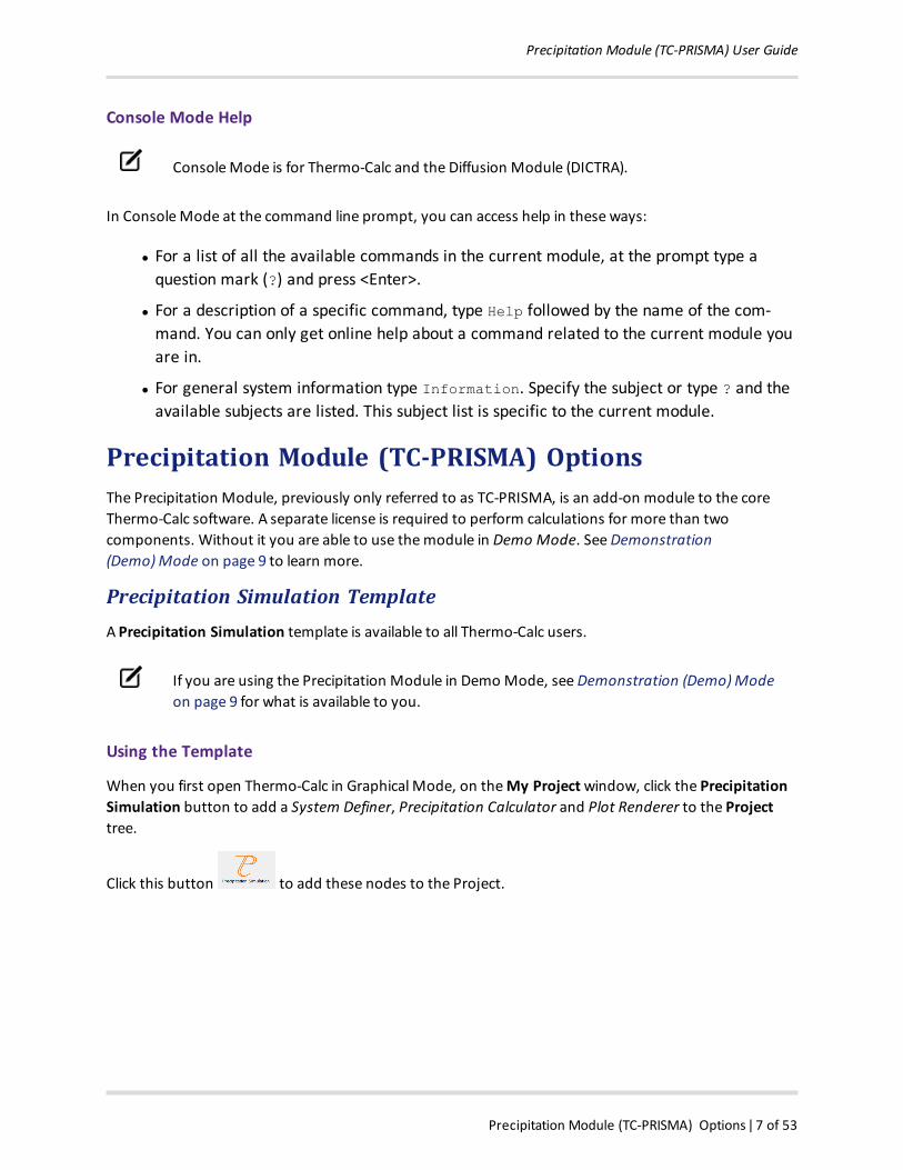
When you first open Thermo-Calc in Graphical Mode, on theMy Projectwindow, click the PrecipitationSimulation button to add a System Definer, Precipitation Calculator and Plot Renderer to the Projecttree.

Click this button to add these nodes to the Project.


Precipitation Calculator ǀ 8 of 53

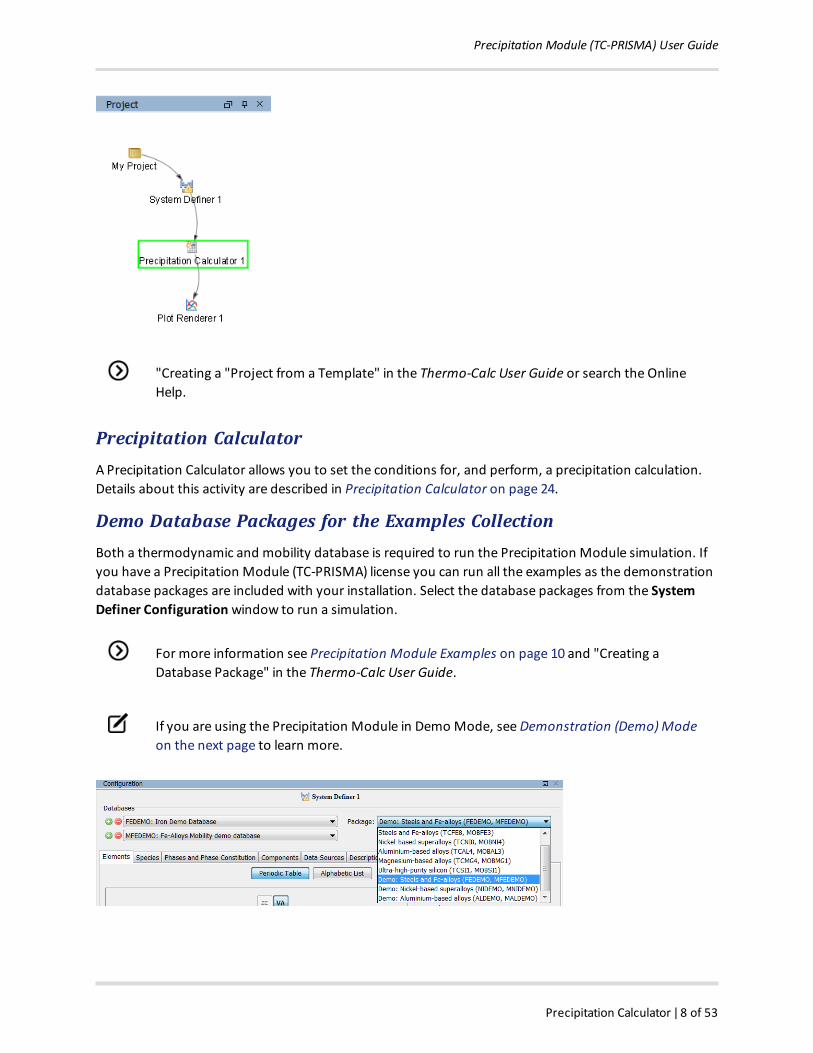
"Creating a "Project from a Template" in the Thermo-Calc User Guide or search the OnlineHelp.

Precipitation CalculatorA Precipitation Calculator allows you to set the conditions for, and perform, a precipitation calculation.Details about this activity are described in Precipitation Calculator on page 24.

Demo Database Packages for the Examples CollectionBoth a thermodynamic and mobility database is required to run the Precipitation Module simulation. Ifyou have a Precipitation Module (TC-PRISMA) license you can run all the examples as the demonstrationdatabase packages are included with your installation. Select the database packages from the SystemDefiner Configurationwindow to run a simulation.

For more information see Precipitation Module Examples on page 10 and "Creating aDatabase Package" in the Thermo-Calc User Guide.

If you are using the Precipitation Module in Demo Mode, seeDemonstration (Demo) Modeon the next page to learn more.


Demonstration (Demo) Mode ǀ 9 of 53

Demonstration (Demo) ModeThe Precipitation Module, and two examples (see Precipitation Module Examples on the next page), areavailable to all Thermo-Calc users but only for simulations with two components. If you do not have alicense for the Precipitation Module then you are in Demonstration Modewhen using the PrecipitationCalculator or Precipitation Simulation template.

Precipitation Simulation Template

When you are in DEMO mode, in the Templates area this is indicated by the text under the logo.

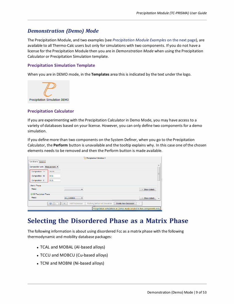
Precipitation Calculator

If you are experimenting with the Precipitation Calculator in Demo Mode, you may have access to avariety of databases based on your license. However, you can only define two components for a demosimulation.

If you definemore than two components on the System Definer, when you go to the PrecipitationCalculator, the Perform button is unavailable and the tooltip explains why. In this case one of the chosenelements needs to be removed and then the Perform button is made available.

Selecting the Disordered Phase as a Matrix PhaseThe following information is about using disordered Fcc as a matrix phase with the followingthermodynamic and mobility database packages:

l TCAL and MOBAL (Al-based alloys)

l TCCU and MOBCU (Cu-based alloys)

l TCNI and MOBNI (Ni-based alloys)


Precipitation Module Examples ǀ 10 of 53

In the TCNI/MOBNI, TCAL/MOBAL, and TCCU/MOBCU packages, the well-known order/disorder two-sublattice model is used to describe the Gibbs energy of both FCC_A1 and FCC_L12. With this treatment,FCC_L12 is becoming FCC_A1 if the site fractions of each element on both sublattices are identical, whichmeans that FCC_A1 is only a special case of FCC_L12. Therefore, FCC_A1 is not shown in the phase list onthe Phases and Phase Constitution tab on the System Definer activity and in subsequent equilibriumcalculation results. Instead it is shown only as FCC_L12. The real ordered FCC_L12 is shown as FCC_L12#2.

In precipitation simulations, thematrix phase is quite often the disordered FCC phase. You can directlyselect FCC_L12 as thematrix phase and run a simulation. However, the speed is not optimal due to thesophisticated model used for both Gibbs energy and atomic mobilities. A better and more convenientway is to deselect FCC_L12 and FCC_L12#2 from the phase list on the Phases and Phase Constitution tabon the System Definer if the ordered phase is irrelevant in the alloy under investigation, such as in mostAl and Cu alloys. Once these are unchecked (i.e. not selected), the FCC_A1 phase is available and can laterbe selected as thematrix phase.

For Ni-based superalloys using the TCNI/MOBNI package, the ordered FCC_L12#2 (gamma prime) has tobe included as the precipitate phase in most of calculations. In this case, you can select DIS_FCC_A1 fromthe phase list on the Phases and Phase Constitution tab and then select it as thematrix phase in thePrecipitation Calculator.

Precipitation Module ExamplesThe Precipitation Module examples are included with theGraphicalMode Example Collection, which youcan find by searching the Online Help. Below are the descriptions of the examples specific to using thePrecipitation Calculator.

Examples 13 and 16 are available to all users. The other examples require a PrecipitationModule (TC-PRISMA) license to calculate and plot results.

All examples use demonstration database packages included with your installation.

Example 13: Isothermal Precipitation of Al3Sc

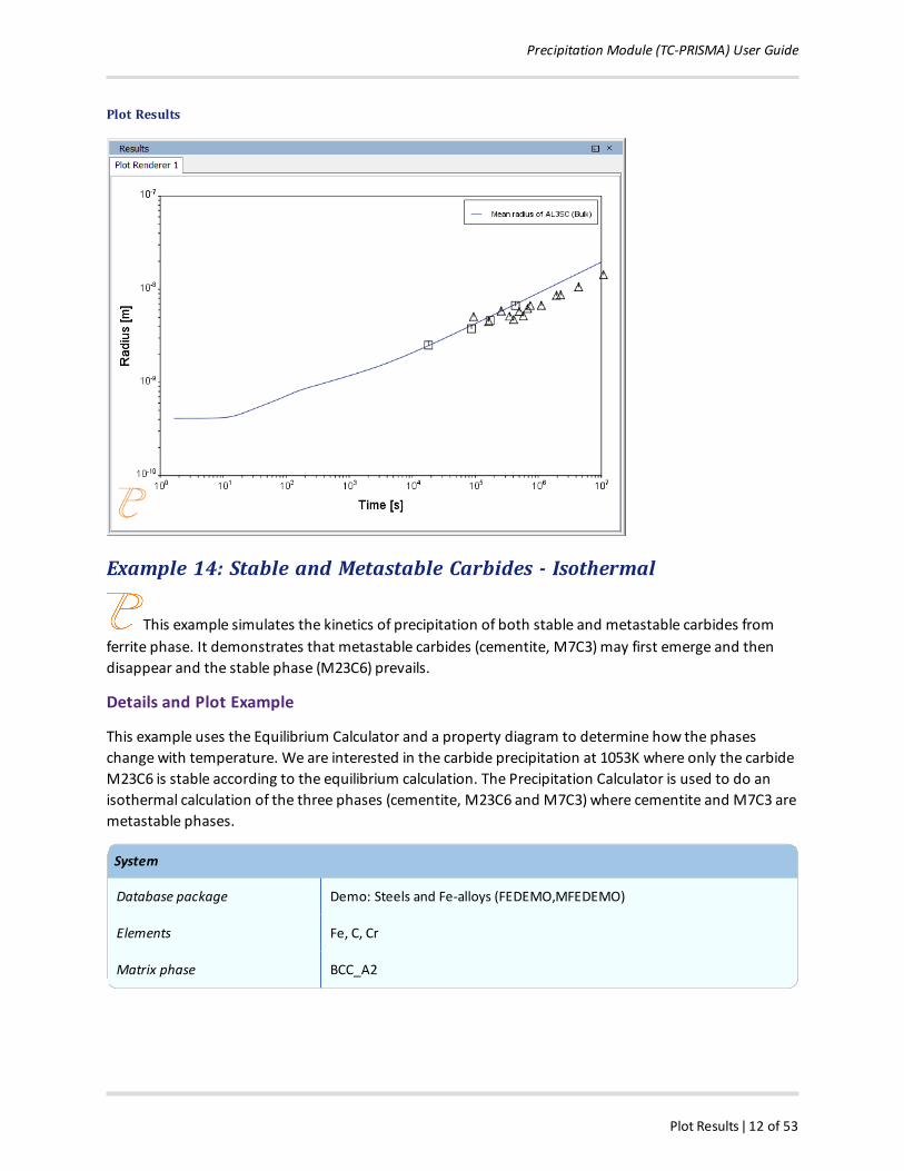
This example simulates the kinetics of precipitation of Al3Sc from an FCC_A1 solution phase. Thesimulation results can be compared with experimental data collected from Marquis and Seidman1 andNovotny and Ardell2.

Details and Plot Example

1E. Marquis, D.. Seidman, Nanoscale structural evolution of Al3Sc precipitates in Al(Sc) alloys, Acta Mater. 49 (2001) 1909–1919.2G.M. Novotny, A.J. Ardell, Precipitation of Al3Sc in binary Al–Sc alloys, Mater. Sci. Eng. A Struct. Mater. Prop. Microstruct.Process. 318 (2001) 144–154.


Example 13: Isothermal Precipitation of Al3Sc ǀ 11 of 53

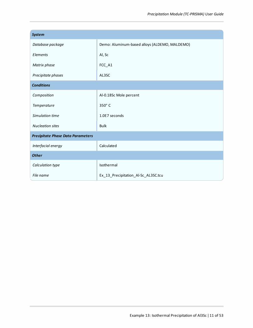
System

Database package Demo: Aluminum-based alloys (ALDEMO, MALDEMO)

Elements Al, Sc

Matrix phase FCC_A1

Precipitate phases AL3SC

Conditions

Composition Al-0.18Sc Mole percent

Temperature 350° C

Simulation time 1.0E7 seconds

Nucleation sites Bulk

Precipitate Phase Data Parameters

Interfacial energy Calculated

Other

Calculation type Isothermal

File name Ex_13_Precipitation_Al-Sc_AL3SC.tcu


Plot Results ǀ 12 of 53

Plot Results

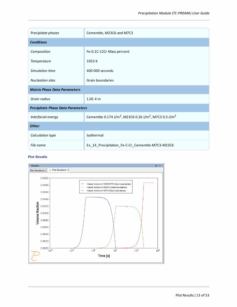
Example 14: Stable and Metastable Carbides - Isothermal

This example simulates the kinetics of precipitation of both stable and metastable carbides fromferrite phase. It demonstrates that metastable carbides (cementite, M7C3)may first emerge and thendisappear and the stable phase (M23C6) prevails.


This example uses the Equilibrium Calculator and a property diagram to determine how the phaseschange with temperature. We are interested in the carbide precipitation at 1053K where only the carbideM23C6 is stable according to the equilibrium calculation. The Precipitation Calculator is used to do anisothermal calculation of the three phases (cementite, M23C6 and M7C3) where cementite and M7C3 aremetastable phases.

System

Database package Demo: Steels and Fe-alloys (FEDEMO,MFEDEMO)

Elements Fe, C, Cr

Matrix phase BCC_A2



Precipitate phases Cementite, M23C6 and M7C3

Conditions

Composition Fe-0.1C-12Cr Mass percent

Temperature 1053 K

Simulation time 400 000 seconds

Nucleation sites Grain boundaries

Matrix Phase Data Parameters

Grain radius 1.0E-4 m


Interfacial energy Cementite 0.174 J/m2, M23C6 0.26 J/m2, M7C3 0.3 J/m2

Other


File name Ex_14_Precipitation_Fe-C-Cr_Cementite-M7C3-M23C6

Plot Results


Example 15: Stable and Metastable Carbides - TTT Diagram ǀ 14 of 53

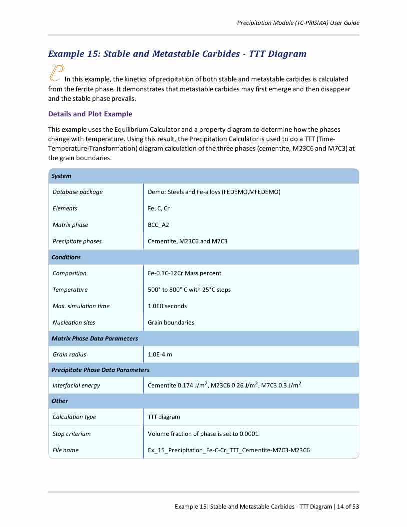
Example 15: Stable and Metastable Carbides - TTT Diagram

In this example, the kinetics of precipitation of both stable and metastable carbides is calculatedfrom the ferrite phase. It demonstrates that metastable carbides may first emerge and then disappearand the stable phase prevails.


This example uses the Equilibrium Calculator and a property diagram to determine how the phaseschange with temperature. Using this result, the Precipitation Calculator is used to do a TTT (Time-Temperature-Transformation) diagram calculation of the three phases (cementite, M23C6 and M7C3) atthe grain boundaries.

System


Elements Fe, C, Cr

Matrix phase BCC_A2

Precipitate phases Cementite, M23C6 and M7C3

Conditions

Composition Fe-0.1C-12Cr Mass percent

Temperature 500° to 800° C with 25°C steps

Max. simulation time 1.0E8 seconds

Nucleation sites Grain boundaries


Grain radius 1.0E-4 m


Interfacial energy Cementite 0.174 J/m2, M23C6 0.26 J/m2, M7C3 0.3 J/m2

Other

Calculation type TTT diagram

Stop criterium Volume fraction of phase is set to 0.0001

File name Ex_15_Precipitation_Fe-C-Cr_TTT_Cementite-M7C3-M23C6



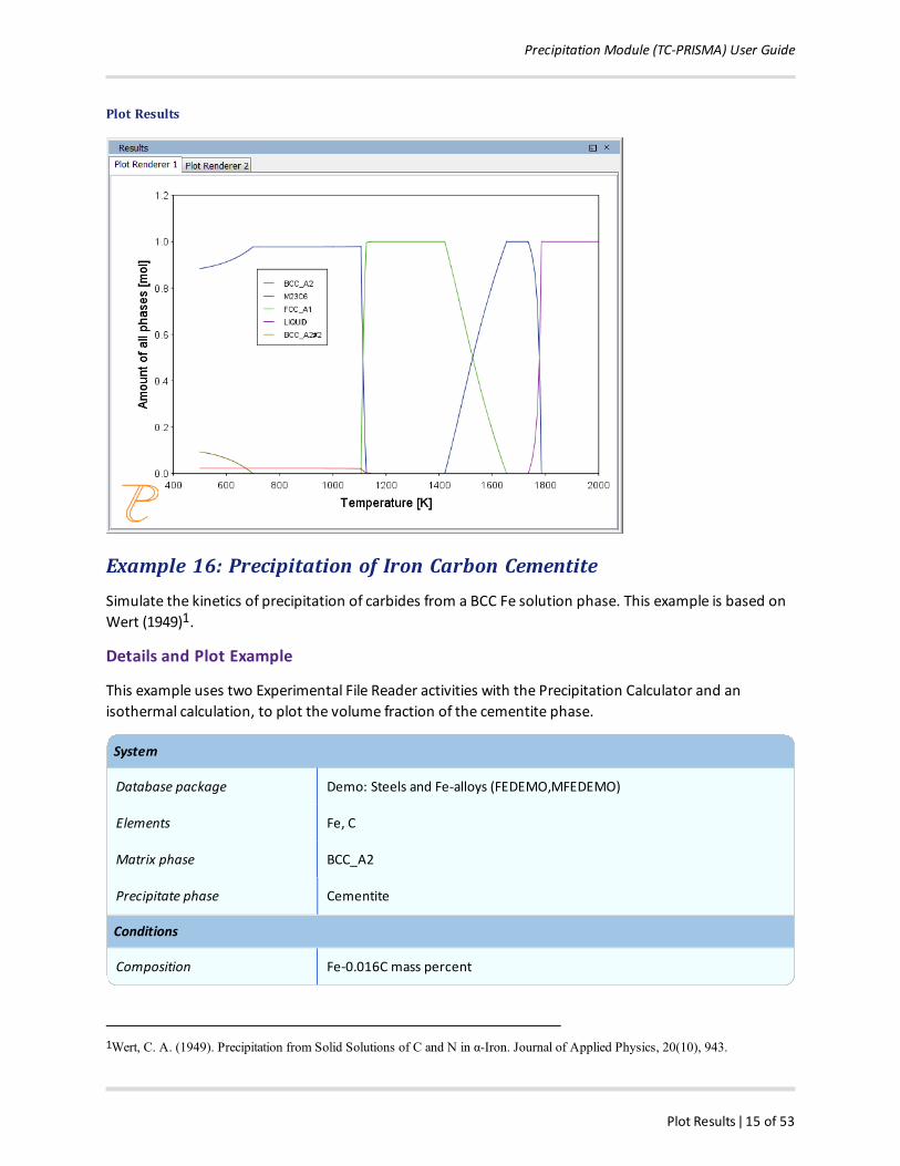
Plot Results

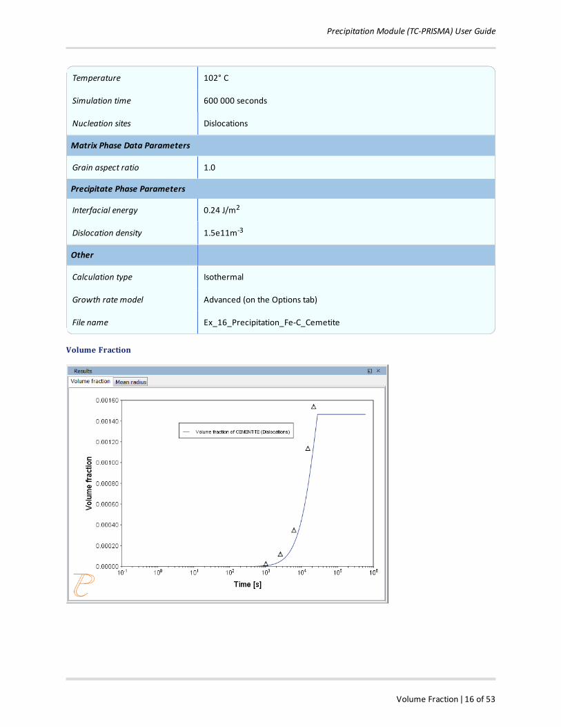
Example 16: Precipitation of Iron Carbon CementiteSimulate the kinetics of precipitation of carbides from a BCC Fe solution phase. This example is based onWert (1949)1.


This example uses two Experimental File Reader activities with the Precipitation Calculator and anisothermal calculation, to plot the volume fraction of the cementite phase.

System


Elements Fe, C

Matrix phase BCC_A2

Precipitate phase Cementite

Conditions

Composition Fe-0.016C mass percent

1Wert, C. A. (1949). Precipitation from Solid Solutions of C and N in α-Iron. Journal of Applied Physics, 20(10), 943.


Volume Fraction ǀ 16 of 53

Temperature 102° C

Simulation time 600 000 seconds

Nucleation sites Dislocations


Grain aspect ratio 1.0

Precipitate Phase Parameters

Interfacial energy 0.24 J/m2

Dislocation density 1.5e11m-3

Other


Growth rate model Advanced (on the Options tab)

File name Ex_16_Precipitation_Fe-C_Cemetite

Volume Fraction


Example 17: Precipitation of g’ in Ni Superalloys - Isothermal ǀ 17 of 53

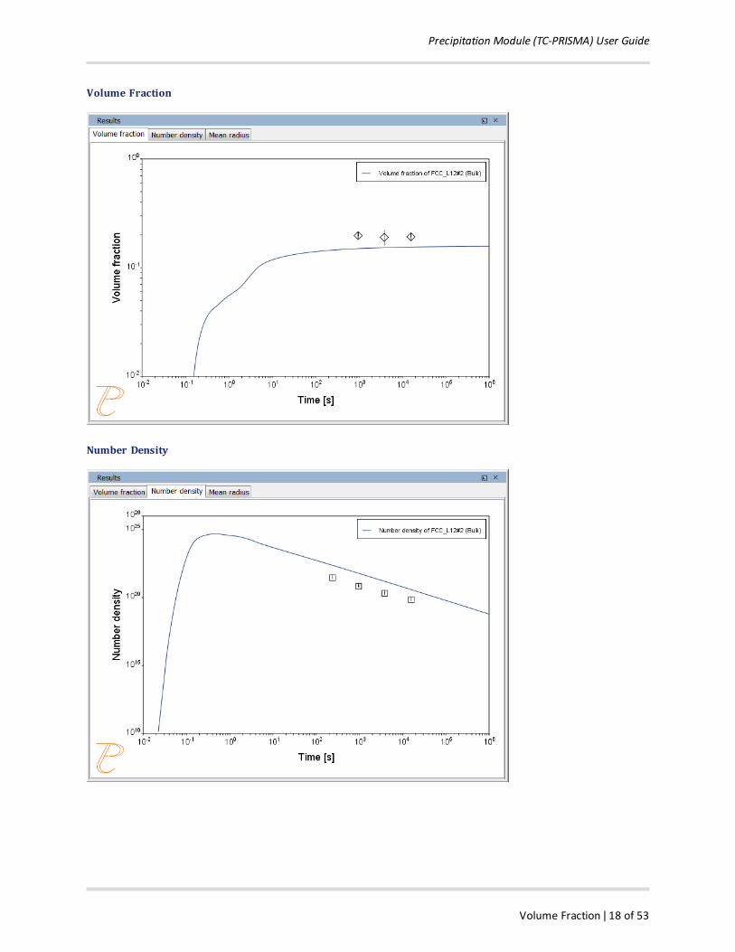
Example 17: Precipitation of γ’ in Ni Superalloys - Isothermal

This example simulates the kinetics of precipitation of γ’ phase from γ phase. The simulation resultscan be compared with experimental data collected from Sudbrack et al.1.

Details and Plot Examples

This example uses three Experimental File Reader activities with the Precipitation Calculator. It does anisothermal calculation to plot the volume fraction, mean radius and number density of the cementitephase.

DIS_FCC_A1 needs to be selected on the System Definer. Search the online help for AboutOrdered Phases in the Precipitation Module (TC-PRISMA) User Guide for details.

System

Database package Demo: Nickel-based Super Alloys (NIDEMO and MNIDEMO)

Elements Ni, Al Cr

Matrix phase DIS-FCC_A1 (see note above about how to select this phase)

Precipitate phase FCC_L12#2

Conditions

Composition Ni-9.8Al-8.3Cr Mole percent

Temperature 800° C

Simulation time 1 000 000 seconds




Other


File name Ex_17_Precipitation_Ni-Al-Cr_Isothermal_Gamma-Gamma_prime

1C.K. Sudbrack, T.D. Ziebell, R.D. Noebe, D.N. Seidman, Effects of a tungsten addition on the morphological evolution, spatial cor-relations and temporal evolution of a model Ni–Al–Cr superalloy, Acta Mater. 56 (2008) 448–463.


Volume Fraction ǀ 18 of 53

Volume Fraction

Number Density


Mean Radius ǀ 19 of 53

Mean Radius

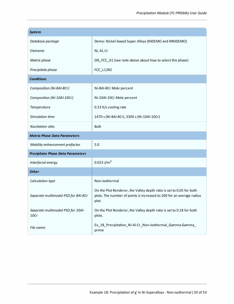
Example 18: Precipitation of γ’ in Ni Superalloys - Non-isothermal

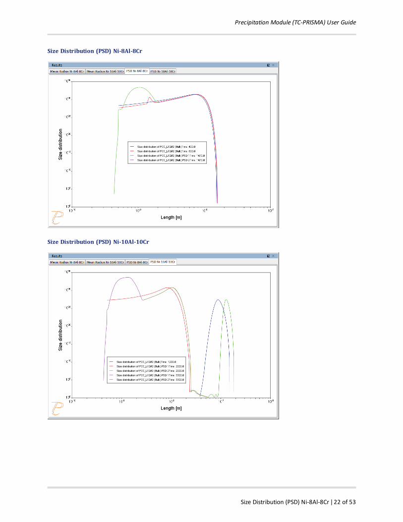
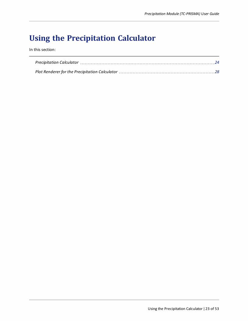
This example simulates the kinetics of precipitation of γ’ phase from γ phase in Ni-8Al-8Cr and Ni-10Al-10Cr at.% alloys during continuous cooling. The simulation results can be compared withexperimental results from Rojhirunsakool et al.1 .

Details and Plot Examples

In these examples the Separatemultimodal PSD check box is selected on the Plot Render to plot themean radius and size distributions of the two compositions.

Plotting the size distribution from the final simulation time of 1470 seconds, you can see there are severalpeaks, although these are not completely separated. Use the 'Separatemultimodal PSD' check box onthe Plot Renderer to separate the peaks. Then adjust the Valley depth ratio setting to 0.05 to separateinto two peaks as shown in the Ni-10Al-10Cr plot example. You can experiment with this setting to seehow the size distribution evolves with time, for example, try entering several values as plot times '400 6001470'.

DIS_FCC_A1 needs to be selected on the System Definer. Search the online help for AboutOrdered Phases in the Precipitation Module (TC-PRISMA) User Guide for details.

1T. Rojhirunsakool, S. Meher, J.Y. Hwang, S. Nag, J. Tiley, R. Banerjee, Influence of composition on monomodal versus mul-timodal γ′ precipitation in Ni–Al–Cr alloys, J. Mater. Sci. 48 (2013) 825–831.


Example 18: Precipitation of g’ in Ni Superalloys - Non-isothermal ǀ 20 of 53

System

Database package Demo: Nickel-based Super Alloys (NIDEMO and MNIDEMO)

Elements Ni, Al, Cr

Matrix phase DIS_FCC_A1 (see note above about how to select this phase)

Precipitate phase FCC_L12#2

Conditions

Composition (Ni-8Al-8Cr) Ni-8Al-8Cr Mole percent

Composition (Ni-10Al-10Cr) Ni-10Al-10Cr Mole percent

Temperature 0.23 K/s cooling rate

Simulation time 1470 s (Ni-8Al-8Cr), 3300 s (Ni-10Al-10Cr)



Mobility enhancement prefactor 5.0



Other

Calculation type Non-isothermal

Separate multimodal PSD for 8Al-8CrOn the Plot Renderer, the Valley depth ratio is set to 0.05 for bothplots. The number of points is increased to 200 for an average radiusplot.

Separate multimodal PSD for 10Al-10Cr

On the Plot Renderer, the Valley depth ratio is set to 0.18 for bothplots.

File nameEx_18_Precipitation_Ni-Al-Cr_Non-isothermal_Gamma-Gamma_prime


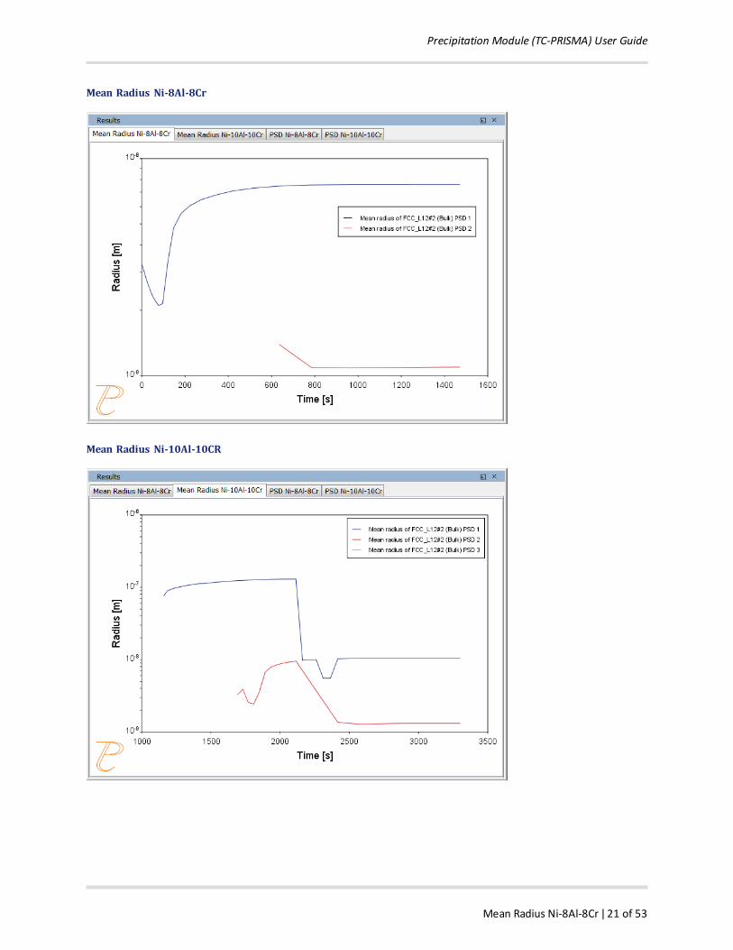
Mean Radius Ni-8Al-8Cr ǀ 21 of 53

Mean Radius Ni-8Al-8Cr

Mean Radius Ni-10Al-10CR


Size Distribution (PSD) Ni-8Al-8Cr ǀ 22 of 53

Size Distribution (PSD) Ni-8Al-8Cr

Size Distribution (PSD) Ni-10Al-10Cr


Using the Precipitation Calculator ǀ 23 of 53

Using the Precipitation CalculatorIn this section:


Plot Renderer for the Precipitation Calculator 28


Precipitation Calculator ǀ 24 of 53

Precipitation Calculator

The Precipitation Calculator is available with two components if you do not have theadditional Precipitation Module (TC-PRISMA) license. With the add-on module you can useall available components.

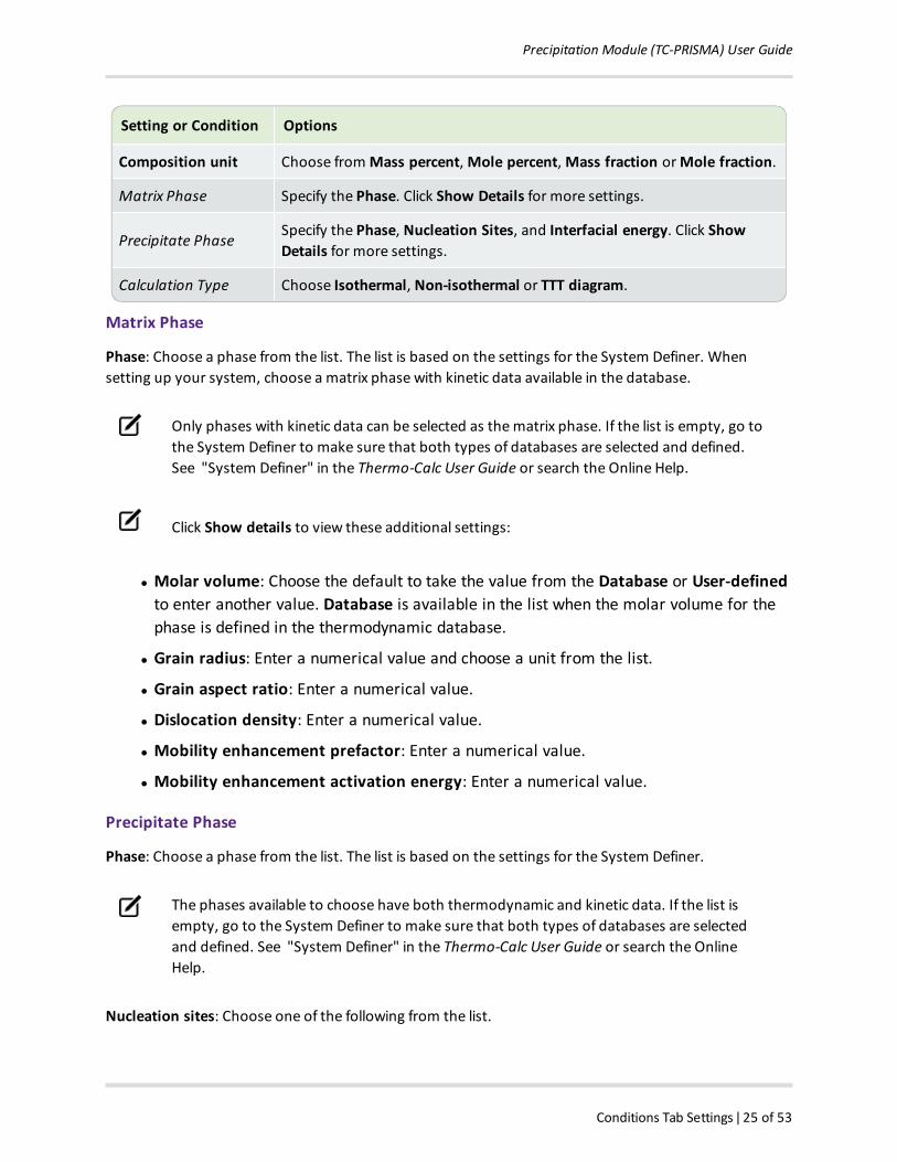
A Precipitation Calculator allows you to set the conditions for, and perform, a precipitation calculation.The Configuration window for a Precipitation Calculator has these tabs:

l Conditions: Set the conditions for your calculation that define the Matrix and Pre-cipitate phases. Choose the Calculation Type.

l Options: Modify Numerical Parameters that determine how the conditions are cal-culated. The Growth rate model can be viewed in Simplified or Advanced mode.

Configuration WindowExample

Conditions Tab SettingsThese are the settings on the Precipitation Calculator Conditions tab.


Conditions Tab Settings ǀ 25 of 53

Setting or Condition Options

Composition unit Choose fromMass percent,Mole percent,Mass fraction orMole fraction.

Matrix Phase Specify the Phase. Click Show Details for more settings.

Precipitate PhaseSpecify the Phase, Nucleation Sites, and Interfacial energy. Click ShowDetails for more settings.

Calculation Type Choose Isothermal, Non-isothermal or TTT diagram.

Matrix Phase

Phase: Choose a phase from the list. The list is based on the settings for the System Definer. Whensetting up your system, choose a matrix phase with kinetic data available in the database.

Only phases with kinetic data can be selected as thematrix phase. If the list is empty, go tothe System Definer to make sure that both types of databases are selected and defined.See "System Definer" in the Thermo-Calc User Guide or search the Online Help.

Click Show details to view these additional settings:

l Molar volume: Choose the default to take the value from the Database or User-definedto enter another value. Database is available in the list when the molar volume for thephase is defined in the thermodynamic database.

l Grain radius: Enter a numerical value and choose a unit from the list.

l Grain aspect ratio: Enter a numerical value.

l Dislocation density: Enter a numerical value.

l Mobility enhancement prefactor: Enter a numerical value.

l Mobility enhancement activation energy: Enter a numerical value.

Precipitate Phase

Phase: Choose a phase from the list. The list is based on the settings for the System Definer.

The phases available to choose have both thermodynamic and kinetic data. If the list isempty, go to the System Definer to make sure that both types of databases are selectedand defined. See "System Definer" in the Thermo-Calc User Guide or search the OnlineHelp.

Nucleation sites: Choose one of the following from the list.


Isothermal ǀ 26 of 53

l Bulk, Grain boundaries, Grain edges, Grain corners, or Dislocations. Click to select theCalculate from matrix settings check box if you want to calculate the number density ofsites.

l For Grain boundaries, Grain edges and Grain corners, enter the Wetting angle in addi-tion to the matrix settings.

l To enter a specific value for the number of nucleation sites, deselect the check box.

Interfacial energy: Choose Calculated to use the estimated value and then enter a different prefactorvalue if you want to adjust the estimated value. You can also chooseUser defined to enter a value inJ/m2.

Click Show details to view these additional settings:

l Molar volume: Choose the default to take the value from the Database or User-definedto enter another value. Database is available in the list when the molar volume for thephase is defined in the thermodynamic database.

l Phase boundary mobility: Enter a numerical value.

l Phase energy addition: Enter a numerical value.

l Approximate driving force: Select the check box to include this if simulations with sev-eral compositions sets of the same phase create problems. See the theory for .

Calculation Type

Isothermal

Use an Isothermal calculation type to do a precipitation simulation at constant temperature.

For the Isothermal calculation type, enter a Temperature and Simulation time.

Non-Isothermal

For theNon-isothermal calculation type, select a Temperature unit and Time unit from the lists. Enter avalue for the Simulation time.

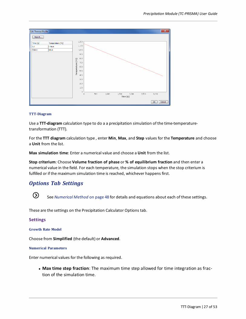
Click Thermal Profile to define the heat treatment schedule. Here the Temperature and Timecoordinates of thermal profile points are entered. Aminimum of two points is required. You can also clickImport to add your own thermal profile from an Excel spreadsheet.

Edit Thermal Profile Window


TTT-Diagram ǀ 27 of 53

TTT-Diagram

Use a TTT-diagram calculation type to do a a precipitation simulation of the time-temperature-transformation (TTT).

For the TTT diagram calculation type , enterMin,Max, and Step values for the Temperature and choosea Unit from the list.

Max simulation time: Enter a numerical value and choose a Unit from the list.

Stop criterium: Choose Volume fraction of phase or% of equilibrium fraction and then enter anumerical value in the field. For each temperature, the simulation stops when the stop criterium isfulfilled or if themaximum simulation time is reached, whichever happens first.

Options Tab Settings

SeeNumerical Method on page 48 for details and equations about each of these settings.

These are the settings on the Precipitation Calculator Options tab.

Settings

Growth Rate Model

Choose from Simplified (the default) or Advanced.

Numerical Parameters

Enter numerical values for the following as required.

l Max time step fraction: The maximum time step allowed for time integration as frac-tion of the simulation time.


Plot Renderer for the Precipitation Calculator ǀ 28 of 53

l No. of grid points over one order of magnitude in radius: Default number of gridpoints for every order of magnitude in size space.

l Max no. of grid points over one order of magnitude in radius: The maximum allowednumber of grid points in size space.

l Min no. of grid points over one order of magnitude in radius: The minimum allowednumber of grid points in size space.

l Max relative volume fraction of subcritical particles allowed to dissolve in one timestep: The portion of the volume fraction that can be ignored when determining the timestep.

l Max relative radius change: The maximum value allowed for relative radius change inone time step.

l Relative radius change for avoiding class collision: Set a limit on the time step.

l Max overall volume change: This defines the maximum absolute (not ratio) change ofthe volume fraction allowed during one time step.

l Max relative change of nucleation rate in logarithmic scale: This parameter ensuresaccuracy for the evolution of effective nucleation rate.

l Max relative change of critical radius: Used to place a constraint on how fast the crit-ical radium can vary, and thus put a limit on time step

l Min radius for a nucleus to be considered as a particle: The cut-off lower limit of pre-cipitate radius.

l Max time step during heating stages: The upper limit of the time step that has beenenforced in the heating stages.

Plot Renderer for the Precipitation Calculator

The Plot Renderer for the Precipitation Calculator on page 24 has additional functionalitywhen using the non-isothermal calculation type. This is described in this section. Forstandard information, see "Plot Renderer" in the Thermo-Calc User Guide or search for it inthe Online Help.

When doing non-isothermal simulations it is common that particles grow in different generations. Thisresults in multi-modal size distributions. To correctly estimate the properties of these differentgenerations of particles you need to separate the peaks ofmulti-modal distributions.

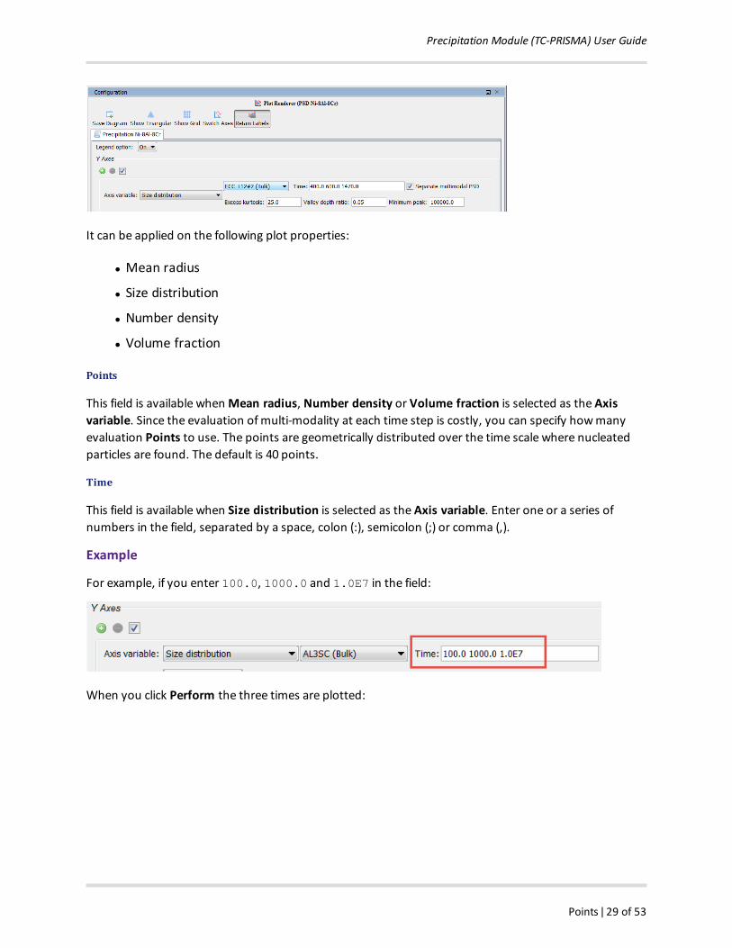
When the Separate multimodal PSD check box is selected on a Plot Renderer activity for thePrecipitation Calculator, the size distribution is evaluated at the given time steps and checked for multi-modal peaks. These are separated and used to calculate the specified property.


Points ǀ 29 of 53

It can be applied on the following plot properties:

l Mean radius

l Size distribution

l Number density

l Volume fraction

Points

This field is available whenMean radius, Number density or Volume fraction is selected as the Axisvariable. Since the evaluation ofmulti-modality at each time step is costly, you can specify howmanyevaluation Points to use. The points are geometrically distributed over the time scale where nucleatedparticles are found. The default is 40 points.

Time

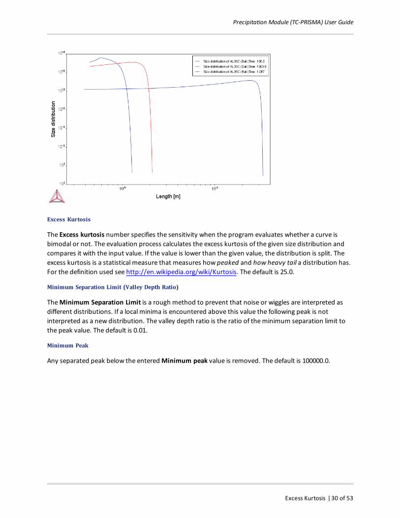
This field is available when Size distribution is selected as the Axis variable. Enter one or a series ofnumbers in the field, separated by a space, colon (:), semicolon (;) or comma (,).

Example

For example, if you enter 100.0, 1000.0 and 1.0E7 in the field:

When you click Perform the three times are plotted:


Excess Kurtosis ǀ 30 of 53

Excess Kurtosis

The Excess kurtosis number specifies the sensitivity when the program evaluates whether a curve isbimodal or not. The evaluation process calculates the excess kurtosis of the given size distribution andcompares it with the input value. If the value is lower than the given value, the distribution is split. Theexcess kurtosis is a statistical measure that measures how peaked and how heavy tail a distribution has.For the definition used see http://en.wikipedia.org/wiki/Kurtosis. The default is 25.0.

Minimum Separation Limit (Valley Depth Ratio)

TheMinimum Separation Limit is a rough method to prevent that noise or wiggles are interpreted asdifferent distributions. If a local minima is encountered above this value the following peak is notinterpreted as a new distribution. The valley depth ratio is the ratio of theminimum separation limit tothe peak value. The default is 0.01.

Minimum Peak

Any separated peak below the enteredMinimum peak value is removed. The default is 100000.0.

http://en.wikipedia.org/wiki/Kurtosis


Theoretical Models ǀ 31 of 53

Theoretical ModelsIn this section:

Theory Overview 32

Nucleation Theory 33

Growth 44

Coarsening 46

Continuity Equation 47

Mass Conservation 47

Numerical Method 48

Interfacial Energy 51

Precipitation Module (TC-PRISMA) References 52


Theory Overview ǀ 32 of 53

Theory OverviewBased on Langer-Schwartz theory1 , Precipitation Module (TC-PRISMA) adopts Kampmann-Wagnernumerical (KWN)method2 to simulate the concomitant nucleation, growth, and coarsening ofprecipitates in multicomponent and multiphase alloy systems. The KWNmethod is an extension of theoriginal Langer-Schwartz (LS) approach and its modified (MLS) form, where the temporal evolution of themean radius and particle density over the whole course of precipitation are predicted by solving a set ofrate equations derived with certain assumptions for the rates of nucleation and growth, as well as thefunction of particle size distribution (PSD). TheMLS approach differs from the LS with respect to theGibbs-Thomson equations used for calculating equilibrium solubilities of small particles. The formerapplies the exact exponential form, whereas the latter takes the convenient linearized version. Instead ofassuming a PSD function a priori and working with rate equations for determining only mean radius andparticle density, the KWNmethod extends the LS and MLS approaches by discretizing the PSD andsolving the continuity equation of the PSD directly. Therefore, the time evolution of the PSD and its nth

moment (0: number density; 1st: mean radius; 3rd: volume fraction) can be obtained altogether duringthe simulation. The key elements of the KWNmethod are themodels for nucleation and growth underthemean field mass balance condition and the numerical algorithm for solving the continuity equation ofthe PSD. Coarsening comes out naturally without any ad hoc treatment.

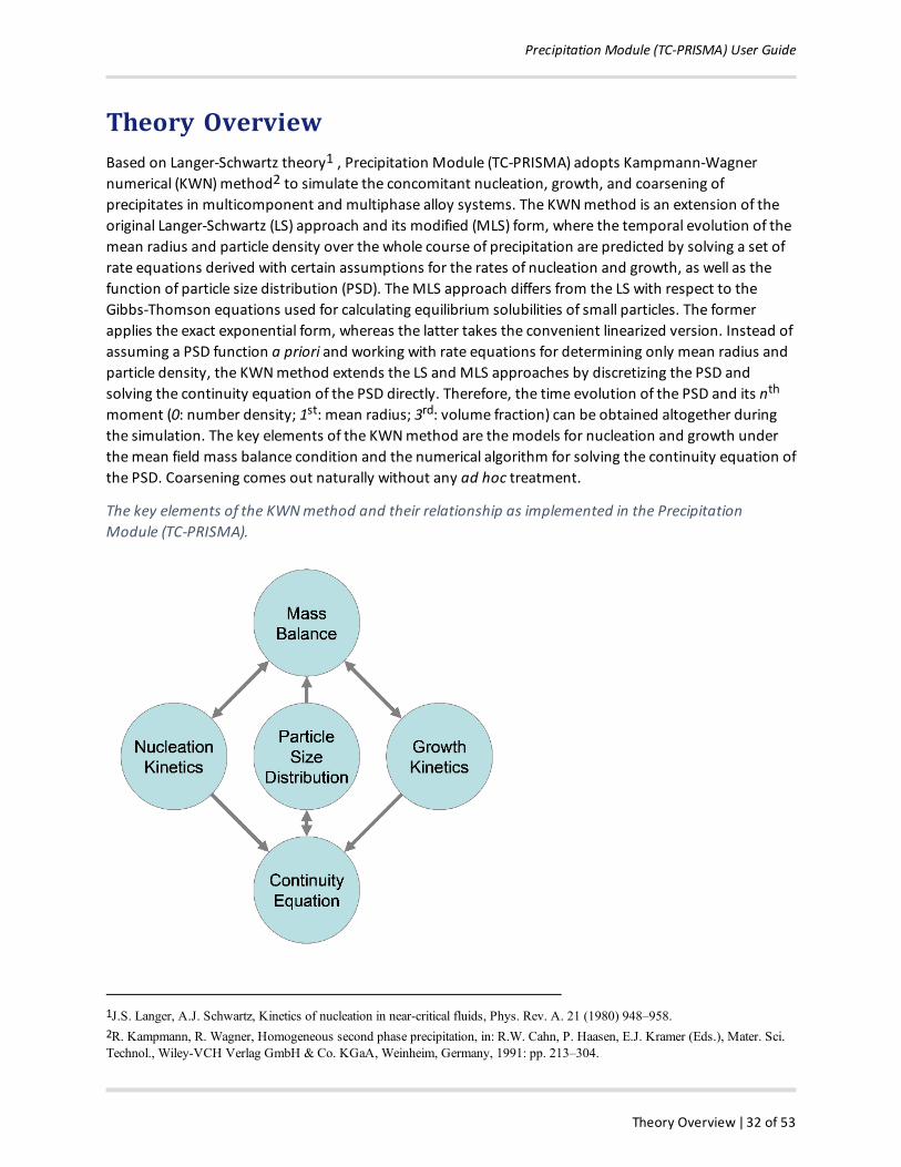
The key elements of the KWNmethod and their relationship as implemented in the PrecipitationModule (TC-PRISMA).

1J.S. Langer, A.J. Schwartz, Kinetics of nucleation in near-critical fluids, Phys. Rev. A. 21 (1980) 948–958.2R. Kampmann, R. Wagner, Homogeneous second phase precipitation, in: R.W. Cahn, P. Haasen, E.J. Kramer (Eds.), Mater. Sci.Technol., Wiley-VCH Verlag GmbH & Co. KGaA, Weinheim, Germany, 1991: pp. 213–304.


Integration of the Precipitation Module into Thermo-Calc ǀ 33 of 53

Integration of the Precipitation Module into Thermo-CalcPrecipitation Module (TC-PRISMA) is integrated with Thermo-Calc in order to directly get all necessarythermodynamic and kinetic information required in the KWNmethod. For industry relevantmulticomponent alloys, thermodynamic and kinetic databases and calculation tools have to be used inorder to obtain various quantities in themulticomponent models for nucleation and growth, such as thedriving forces for the formation of embryos and their compositions, the atomic mobilities or diffusivitiesin thematrix, the operating interface compositions under local equilibrium conditions, the Gibbs-Thomson effect, and the deviation from local equilibrium due to interface friction etc. With Thermo-Calcand the Diffusion Module (DICTRA) as well as the accompanying databases, all these properties andeffects can be calculated without unnecessary and inaccurate approximations.

In the following topics, various models and numerical methods implemented in Precipitation Module(TC-PRISMA) are introduced. Spherical particles are assumed in the discussion. For non-spherical andwetting angle effect, seeHomogeneous Nucleation below.

Nucleation TheoryPrecipitation starts from the nucleation of clusters that can be considered as embryos of new phaseswith distinctive structures or compositions. In a perfect single crystal, nucleation happenshomogeneously. In an imperfect crystal or polycrystallinematerials, nucleation tends to occurheterogeneously due to the presence of dislocations, grain boundaries, grain edges, and grain corners.These imperfections or defects reduce the nucleation barrier and facilitate nucleation. However, ifsupersaturation or driving force is very large homogeneous nucleation is also possible since all sitesincluding those inside a grain can be activated.

l Homogeneous Nucleation below

l Heterogeneous Nucleation on page 37

l Nucleation During a Non-isothermal Process on page 43

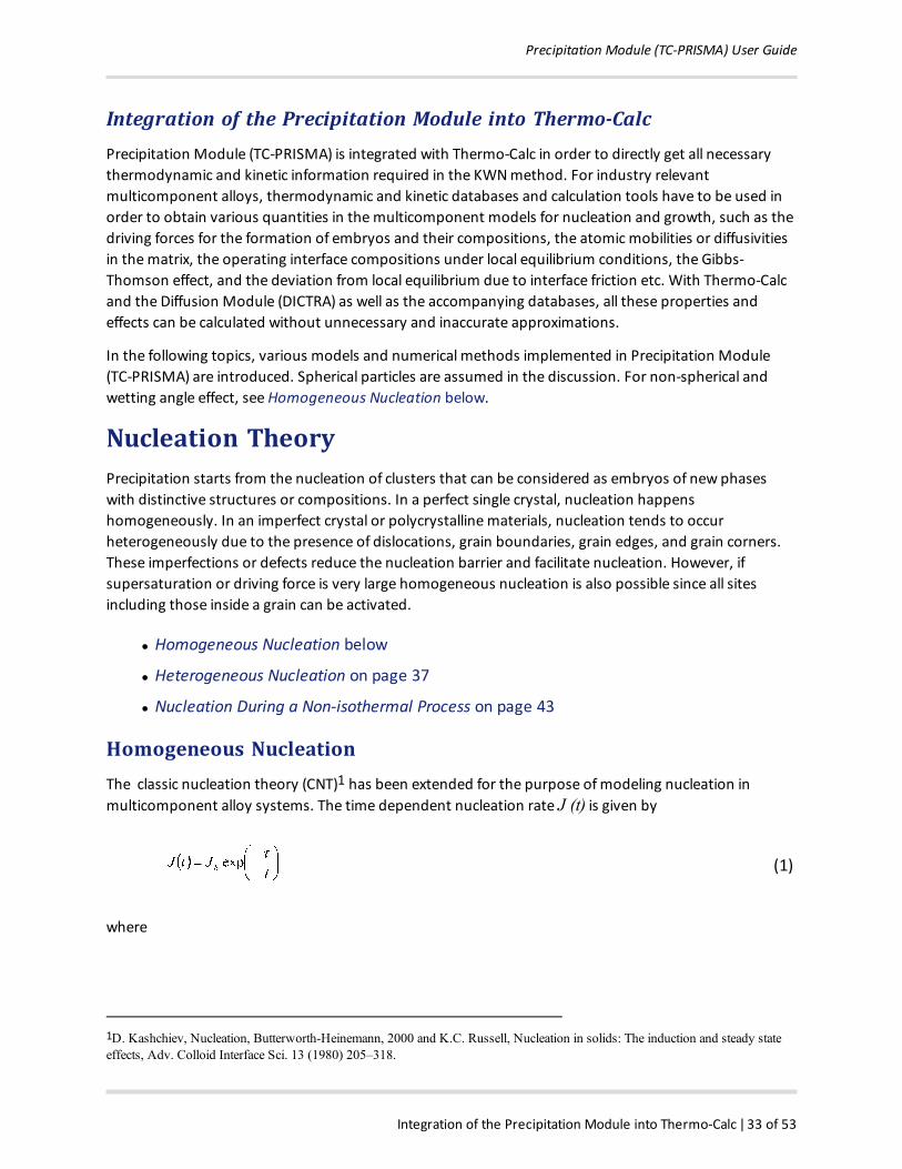
Homogeneous NucleationThe classic nucleation theory (CNT)1 has been extended for the purpose ofmodeling nucleation inmulticomponent alloy systems. The time dependent nucleation rate J (t) is given by

(1)

where

1D. Kashchiev, Nucleation, Butterworth-Heinemann, 2000 and K.C. Russell, Nucleation in solids: The induction and steady stateeffects, Adv. Colloid Interface Sci. 13 (1980) 205–318.


Homogeneous Nucleation ǀ 34 of 53

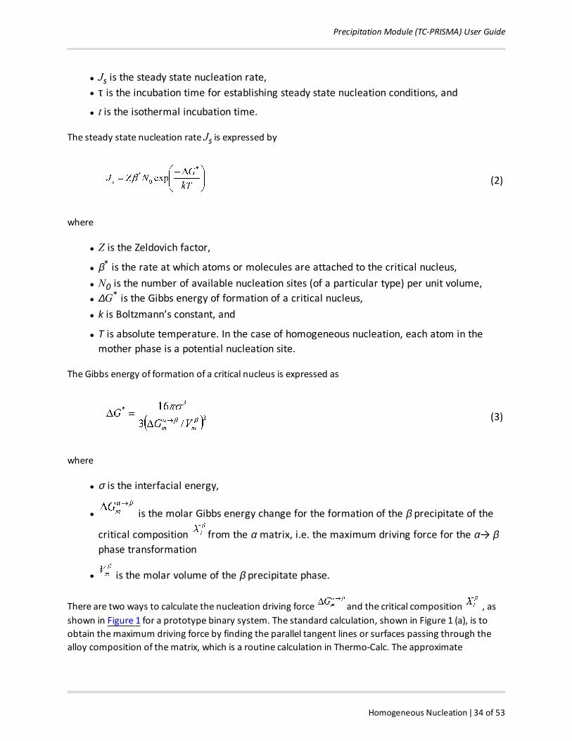
l Js is the steady state nucleation rate,l τ is the incubation time for establishing steady state nucleation conditions, and

l t is the isothermal incubation time.

The steady state nucleation rate Js is expressed by

(2)

where

l Z is the Zeldovich factor,

l β* is the rate at which atoms or molecules are attached to the critical nucleus,l N0 is the number of available nucleation sites (of a particular type) per unit volume,l ∆G* is the Gibbs energy of formation of a critical nucleus,l k is Boltzmann’s constant, and

l T is absolute temperature. In the case of homogeneous nucleation, each atom in themother phase is a potential nucleation site.

The Gibbs energy of formation of a critical nucleus is expressed as

(3)

where

l σ is the interfacial energy,

l is the molar Gibbs energy change for the formation of the β precipitate of the

critical composition from the α matrix, i.e. the maximum driving force for the α→ βphase transformation

l is the molar volume of the β precipitate phase.

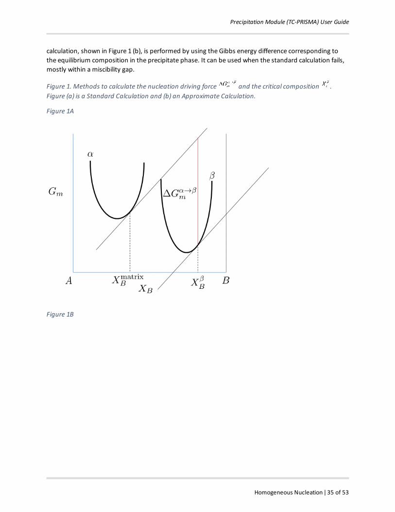
There are two ways to calculate the nucleation driving force and the critical composition , asshown in Figure 1 for a prototype binary system. The standard calculation, shown in Figure 1 (a), is toobtain themaximum driving force by finding the parallel tangent lines or surfaces passing through thealloy composition of thematrix, which is a routine calculation in Thermo-Calc. The approximate



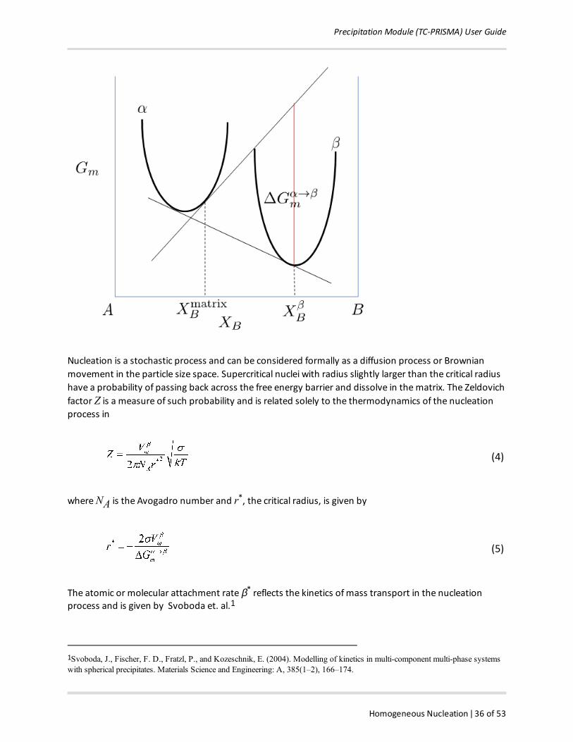
calculation, shown in Figure 1 (b), is performed by using the Gibbs energy difference corresponding tothe equilibrium composition in the precipitate phase. It can be used when the standard calculation fails,mostly within a miscibility gap.

Figure 1. Methods to calculate the nucleation driving force and the critical composition .Figure (a) is a Standard Calculation and (b) an Approximate Calculation.

Figure 1A

Figure 1B



Nucleation is a stochastic process and can be considered formally as a diffusion process or Brownianmovement in the particle size space. Supercritical nuclei with radius slightly larger than the critical radiushave a probability of passing back across the free energy barrier and dissolve in thematrix. The Zeldovichfactor Z is a measure of such probability and is related solely to the thermodynamics of the nucleationprocess in

(4)

whereNA is the Avogadro number and r*, the critical radius, is given by

(5)

The atomic or molecular attachment rate β* reflects the kinetics ofmass transport in the nucleationprocess and is given by Svoboda et. al.1

1Svoboda, J., Fischer, F. D., Fratzl, P., and Kozeschnik, E. (2004). Modelling of kinetics in multi-component multi-phase systemswith spherical precipitates. Materials Science and Engineering: A, 385(1–2), 166–174.


Heterogeneous Nucleation ǀ 37 of 53

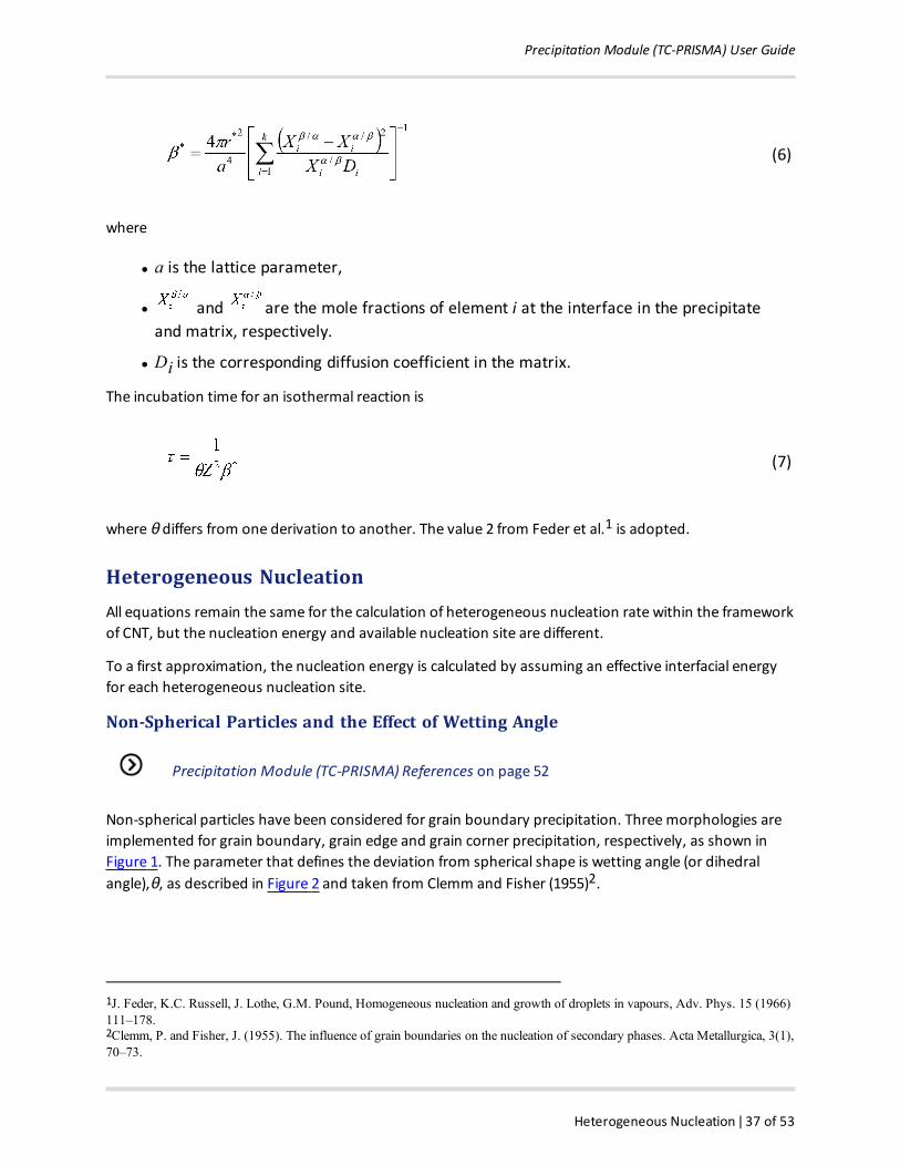
(6)

where

l a is the lattice parameter,

l and are the mole fractions of element i at the interface in the precipitateand matrix, respectively.

l Di is the corresponding diffusion coefficient in the matrix.

The incubation time for an isothermal reaction is

(7)

where θ differs from one derivation to another. The value 2 from Feder et al.1 is adopted.

Heterogeneous NucleationAll equations remain the same for the calculation of heterogeneous nucleation rate within the frameworkof CNT, but the nucleation energy and available nucleation site are different.

To a first approximation, the nucleation energy is calculated by assuming an effective interfacial energyfor each heterogeneous nucleation site.

Non-Spherical Particles and the Effect of Wetting Angle

Precipitation Module (TC-PRISMA) References on page 52

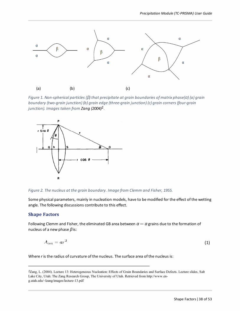
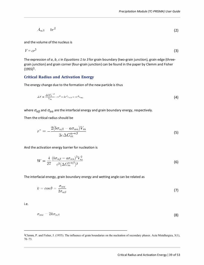
Non-spherical particles have been considered for grain boundary precipitation. Threemorphologies areimplemented for grain boundary, grain edge and grain corner precipitation, respectively, as shown inFigure 1. The parameter that defines the deviation from spherical shape is wetting angle (or dihedralangle),θ, as described in Figure 2 and taken from Clemm and Fisher (1955)2.

1J. Feder, K.C. Russell, J. Lothe, G.M. Pound, Homogeneous nucleation and growth of droplets in vapours, Adv. Phys. 15 (1966)111–178.2Clemm, P. and Fisher, J. (1955). The influence of grain boundaries on the nucleation of secondary phases. Acta Metallurgica, 3(1),70–73.


Shape Factors ǀ 38 of 53

(a) (b) (c)

Figure 1. Non-spherical particles (β) that precipitate at grain boundaries ofmatrix phase(α) (a) grainboundary (two-grain junction) (b) grain edge (three-grain junction) (c) grain corners (four-grainjunction). Images taken from Zang (2004)1.

Figure 2. The nucleus at the grain boundary. Image from Clemm and Fisher, 1955.

Some physical parameters, mainly in nucleation models, have to bemodified for the effect of the wettingangle. The following discussions contribute to this effect.

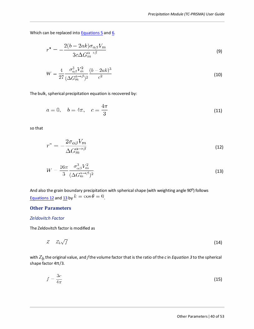
Shape Factors

Following Clemm and Fisher, the eliminated GB area between α — α grains due to the formation ofnucleus of a new phase β is:

(1)

Where r is the radius of curvature of the nucleus. The surface area of the nucleus is:

1Zang, L. (2004). Lecture 13: Heterogeneous Nucleation: Effects of Grain Boundaries and Surface Defects. Lecture slides, SaltLake City, Utah: The Zang Research Group, The University of Utah. Retrieved from http://www.en-g.utah.edu/~lzang/images/lecture-13.pdf


Critical Radius and Activation Energy ǀ 39 of 53

(2)

and the volume of the nucleus is

V = cr3 (3)

The expression of a, b, c in Equations 1 to 3 for grain boundary (two-grain junction), grain edge (three-grain junction) and grain corner (four-grain junction) can be found in the paper by Clemm and Fisher(1955)1.

Critical Radius and Activation Energy

The energy change due to the formation of the new particle is thus

(4)

where σαβ and σαα are the interfacial energy and grain boundary energy, respectively.

Then the critical radius should be

(5)

And the activation energy barrier for nucleation is

(6)

The interfacial energy, grain boundary energy and wetting angle can be related as

(7)

i.e.

(8)

1Clemm, P. and Fisher, J. (1955). The influence of grain boundaries on the nucleation of secondary phases. Acta Metallurgica, 3(1),70–73.


Other Parameters ǀ 40 of 53

Which can be replaced into Equations 5 and 6.

(9)

(10)

The bulk, spherical precipitation equation is recovered by:

(11)

so that

(12)

(13)

And also the grain boundary precipitation with spherical shape (with weighting angle 90o) follows

Equations 12 and 13 by .

Other Parameters

Zeldovitch Factor

The Zeldovitch factor is modified as

(14)

with Zb the original value, and f the volume factor that is the ratio of the c in Equation 3 to the sphericalshape factor 4π /3.

(15)


Impingement Rate ǀ 41 of 53

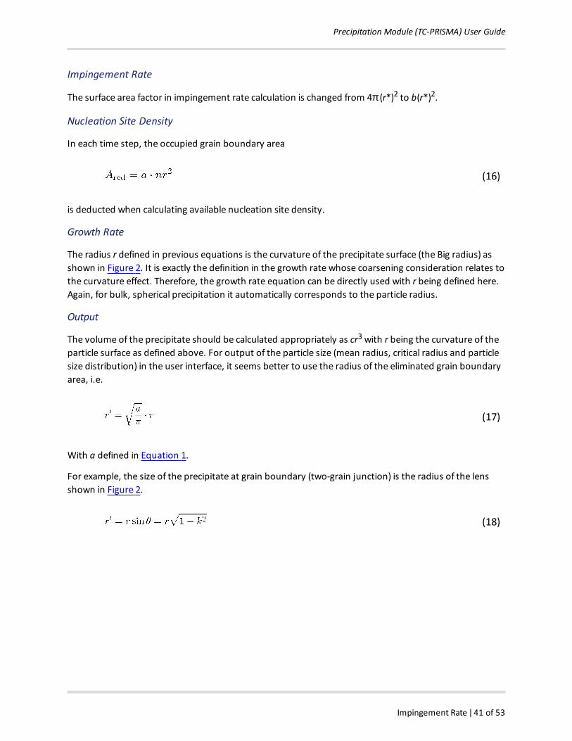
Impingement Rate

The surface area factor in impingement rate calculation is changed from 4π (r*)2 to b(r*)2.

Nucleation Site Density

In each time step, the occupied grain boundary area

(16)

is deducted when calculating available nucleation site density.

Growth Rate

The radius r defined in previous equations is the curvature of the precipitate surface (the Big radius) asshown in Figure 2. It is exactly the definition in the growth rate whose coarsening consideration relates tothe curvature effect. Therefore, the growth rate equation can be directly used with r being defined here.Again, for bulk, spherical precipitation it automatically corresponds to the particle radius.

Output

The volume of the precipitate should be calculated appropriately as cr3with r being the curvature of theparticle surface as defined above. For output of the particle size (mean radius, critical radius and particlesize distribution) in the user interface, it seems better to use the radius of the eliminated grain boundaryarea, i.e.

(17)

With a defined in Equation 1.

For example, the size of the precipitate at grain boundary (two-grain junction) is the radius of the lensshown in Figure 2.

(18)


The Shape and Size of Grains in the Matrix ǀ 42 of 53

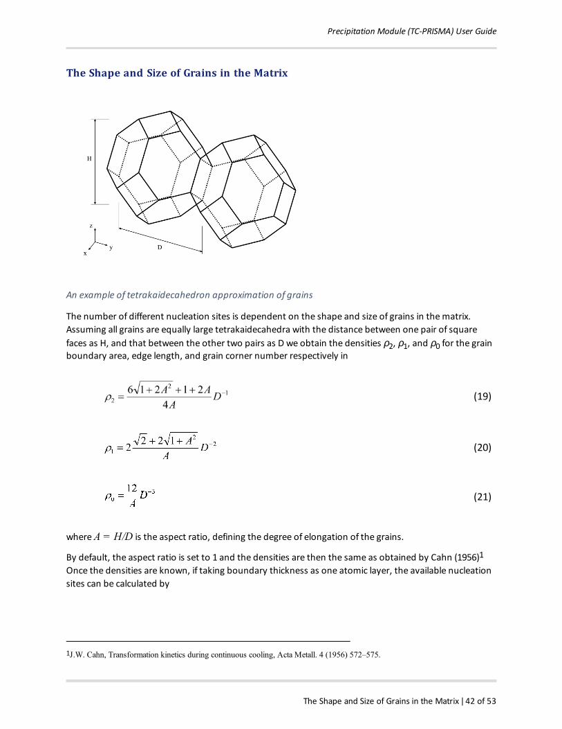
The Shape and Size of Grains in the Matrix

An example of tetrakaidecahedron approximation of grains

The number of different nucleation sites is dependent on the shape and size of grains in thematrix.Assuming all grains are equally large tetrakaidecahedra with the distance between one pair of squarefaces as H, and that between the other two pairs as D we obtain the densities ρ2, ρ1, and ρ0 for the grainboundary area, edge length, and grain corner number respectively in

(19)

(20)

(21)

whereA = H/D is the aspect ratio, defining the degree of elongation of the grains.

By default, the aspect ratio is set to 1 and the densities are then the same as obtained by Cahn (1956)1Once the densities are known, if taking boundary thickness as one atomic layer, the available nucleationsites can be calculated by

1J.W. Cahn, Transformation kinetics during continuous cooling, Acta Metall. 4 (1956) 572–575.


Nucleation During a Non-isothermal Process ǀ 43 of 53

(22)

where is themolar volume of thematrix phase and NAis the Avogadro number.

For a crystallinematerial, given a dislocation density ρd, the number of nucleation sites at thedislocations Nd can be calculated with the same form as in

(23)

Nucleation During a Non-isothermal ProcessUnder a non-isothermal conditions, temperature dependency of key parameters such as nucleationdriving force, solute diffusivities and solute concentrations, etc., have been taken into account, and areupdated automatically during a simulation.

Another important parameter that depends on thermal history is the incubation time, defined by

(1)

for an isothermal condition. In a non-isothermal process, the exact calculation of the incubation timerequires a solution to the Fokker-Plank equation. In the Precipitation Module, an approximationapproach has been employed to deal with the transient nucleation, which gives the incubation time asan integral form of past thermal history1 as in

(2)

where

τ is the incubation time, β*is the impingement rate for solute atoms to the critical cluster as defined in

1H.-J. Jou, P. Voorhees, G.B. Olson, Computer simulations for the prediction of microstructure/property variation in aeroturbinedisks, Superalloys. (2004) 877–886.


Growth ǀ 44 of 53

(3)

and Z is the Zeldovich factor, previously defined in

(4)

but now as a function of τ derived from temperature change.

The starting point of the integral (t' = 0 ) is either the starting time if there is an initial nucleation drivingforce, or the latest timewhen the nucleation driving force is vanished.

GrowthThe growth ratemodels implemented in the Precipitation Module are called Advanced and Simplified.

The Advancedmodel is proposed by Chen, Jeppsson, and Ågren1 (CJA) and calculates the velocity of amoving phase interface in multicomponent systems by identifying the operating tie-line from thesolution of flux-balance equations. This model can treat both high supersaturation and cross diffusionrigorously. Spontaneous transitions between different modes (LE and NPLE) of phase transformation canbe captured without any ad hoc treatment. Since it is not always possible to solve the flux-balanceequations and it takes timewhen possible, a less rigorous but simple and efficient model is preferred inmany applications. The simplified model is based on the advanced model but avoids the difficulty to findthe operating tie-line and uses simply the tie-line across the bulk composition.

All models treat a spherical particle of stoichiometric composition or with negligible atomic diffusivitygrowing under the local equilibrium condition.

According to the CJAmodel, the interface velocity ν can be obtained together with interfaceconcentrations by numerically solving 2n – 1 equations, comprising of the flux balance equations for n – 1independent components and the local equilibrium conditions for all n components as in

(1)

1Q. Chen, J. Jeppsson, J. Ågren, Analytical treatment of diffusion during precipitate growth in multicomponent systems, ActaMater. 56 (2008) 1890–1896.


Growth ǀ 45 of 53

(2)

where

l and are the volume concentrations of component i at the interface in the pre-cipitate and matrix, respectively,

l Mi is the corresponding atomic mobility in the matrix, and

l are the chemical potentials in the matrix of the mean-field concentration and atthe interface, respectively.

l is the chemical potential at the interface in the precipitate.

In the above local equilibrium condition, themulticomponent Gibbs-Thomson effect has been taken intoaccount by adding a curvature induced pressure term to the Gibbs energy of the precipitate phase.

The introduced effective diffusion distance factor, ξi, for each independent component is given by

(3)

where

is the so-called dimensionless supersaturation for an individual component, and λi is obtained via

(4)

Combining Equation 1 and Equation 2, the simplified model is derived in

(5)

where


Coarsening ǀ 46 of 53

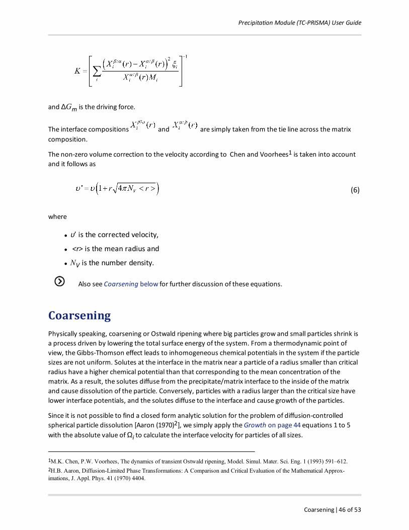
and ∆Gm is the driving force.

The interface compositions and are simply taken from the tie line across thematrixcomposition.

The non-zero volume correction to the velocity according to Chen and Voorhees1 is taken into accountand it follows as

(6)

where

l υ’ is the corrected velocity,

l <r> is the mean radius and

l NV is the number density.

Also see Coarsening below for further discussion of these equations.

CoarseningPhysically speaking, coarsening or Ostwald ripening where big particles grow and small particles shrink isa process driven by lowering the total surface energy of the system. From a thermodynamic point ofview, the Gibbs-Thomson effect leads to inhomogeneous chemical potentials in the system if the particlesizes are not uniform. Solutes at the interface in thematrix near a particle of a radius smaller than criticalradius have a higher chemical potential than that corresponding to themean concentration of thematrix. As a result, the solutes diffuse from the precipitate/matrix interface to the inside of thematrixand cause dissolution of the particle. Conversely, particles with a radius larger than the critical size havelower interface potentials, and the solutes diffuse to the interface and cause growth of the particles.

Since it is not possible to find a closed form analytic solution for the problem of diffusion-controlledspherical particle dissolution [Aaron (1970)2], we simply apply theGrowth on page 44 equations 1 to 5with the absolute value ofΩi to calculate the interface velocity for particles of all sizes.

1M.K. Chen, P.W. Voorhees, The dynamics of transient Ostwald ripening, Model. Simul. Mater. Sci. Eng. 1 (1993) 591–612.2H.B. Aaron, Diffusion-Limited Phase Transformations: A Comparison and Critical Evaluation of the Mathematical Approx-imations, J. Appl. Phys. 41 (1970) 4404.


Continuity Equation ǀ 47 of 53

As can be easily seen, if r < r*, then the Gibbs-Thomson Equation 1 (seeGrowth on page 44) gives

, and a negative velocity results from Equation 2 (seeGrowth on page 44) for particles havingr < r*, which means that they shrink.

Results for particles having r > r* are obtained vice versa. In all situations, when the absolute values of Ωi are very small, the steady-state solution for either growth or dissolution are recovered. In conclusion,the dissolution is treated as the reverse of growth1 , and the coarsening comes out naturally eithertogether with nucleation and growth or as a dominant process finally in the course of the evolution ofthe PSD.

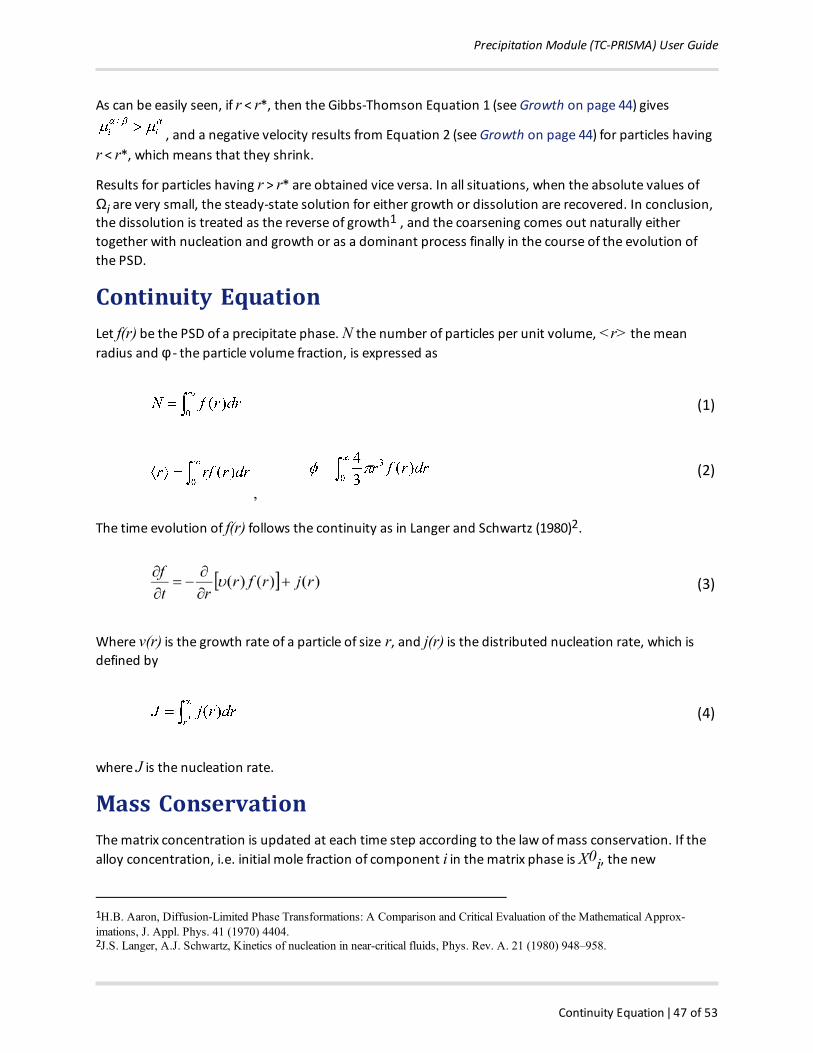
Continuity EquationLet f(r) be the PSD of a precipitate phase. N the number of particles per unit volume, <r> themeanradius and φ - the particle volume fraction, is expressed as

(1)

,(2)

The time evolution of f(r) follows the continuity as in Langer and Schwartz (1980)2.

(3)

Where v(r) is the growth rate of a particle of size r, and j(r) is the distributed nucleation rate, which isdefined by

(4)

where J is the nucleation rate.

Mass ConservationThematrix concentration is updated at each time step according to the law ofmass conservation. If thealloy concentration, i.e. initial mole fraction of component i in thematrix phase is X0i, the new

1H.B. Aaron, Diffusion-Limited Phase Transformations: A Comparison and Critical Evaluation of the Mathematical Approx-imations, J. Appl. Phys. 41 (1970) 4404.2J.S. Langer, A.J. Schwartz, Kinetics of nucleation in near-critical fluids, Phys. Rev. A. 21 (1980) 948–958.


Numerical Method ǀ 48 of 53

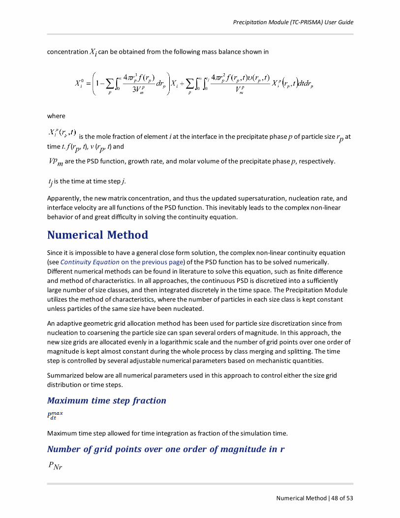
concentration Xi can be obtained from the following mass balance shown in

where

is themole fraction of element i at the interface in the precipitate phase p of particle size rp attime t. f (rp, t), v (rp, t) and

Vpm are the PSD function, growth rate, and molar volume of the precipitate phase p, respectively.

tj is the time at time step j.

Apparently, the newmatrix concentration, and thus the updated supersaturation, nucleation rate, andinterface velocity are all functions of the PSD function. This inevitably leads to the complex non-linearbehavior of and great difficulty in solving the continuity equation.

Numerical MethodSince it is impossible to have a general close form solution, the complex non-linear continuity equation(see Continuity Equation on the previous page) of the PSD function has to be solved numerically.Different numerical methods can be found in literature to solve this equation, such as finite differenceand method of characteristics. In all approaches, the continuous PSD is discretized into a sufficientlylarge number of size classes, and then integrated discretely in the time space. The Precipitation Moduleutilizes themethod of characteristics, where the number of particles in each size class is kept constantunless particles of the same size have been nucleated.

An adaptive geometric grid allocation method has been used for particle size discretization since fromnucleation to coarsening the particle size can span several orders ofmagnitude. In this approach, thenew size grids are allocated evenly in a logarithmic scale and the number of grid points over one order ofmagnitude is kept almost constant during the whole process by class merging and splitting. The timestep is controlled by several adjustable numerical parameters based on mechanistic quantities.

Summarized below are all numerical parameters used in this approach to control either the size griddistribution or time steps.

Maximum time step fraction

Maximum time step allowed for time integration as fraction of the simulation time.

Number of grid points over one order of magnitude in rPNr


Maximum number of grid points over one order of magnitude in r ǀ 49 of 53

Default number of grid points for every order ofmagnitude in size space. The number determines adefault ratio between two adjacent grid points. When there is a need to create new grid points, such asnucleating at a new radius not covered by the current range of PSD, this default ratio is used to add thesenew radius grid points. A larger value of this parameter enforces a finer grid to allow better numericalaccuracy. However, this also comes with performance penalty, since finer grid in the size space oftenrequires smaller time step to resolve the calculations.

Maximum number of grid points over one order of magnitude in r

Themaximum allowed number of grid points in size space. This parameter determines a lower boundlimitation for the ratio of every two next nearest grid points in order to maintain adequatecomputational efficiency. When a ratio of two next nearest grid points is less than this limit, themiddlegrid point is removed and the corresponding size class merged with the two neighbouring ones.

Minimum number of grid points over one order of magnitude in r

Theminimum allowed number of grid points in size space. This parameter determines an upper boundlimitation for the ratio of every two adjacent grid points in order to maintain proper numerical accuracy.When a ratio of two adjacent grid points exceeds this limit, a new grid point is then inserted between thetwo adjacent grids to keep the required resolution.

Maximum relative radius changePr

Themaximum value allowed for relative radius change in one time step. This parameter limits the timestep according to the following relation, which is controlled by the particle growth:

for r > rdt, where rdtis a cut-off subcritical size defined by the next parameter. Thegrowth rates of supercritical particles (with r > rc) are always bounded, and there is a size class and thecorresponding growth rate that controls the time step. The subcritical particles (with r < rc), however,has a mathematical singularity (negative infinity) in growth rate as approaches 0. This means that thetime step can become extremely small if applying the above criterion to very small subcritical particles. Inopen literature, several researchers have tried mathematical transformation to avoid this singularity.Unfortunately, the transformation also complicates the formulation of themodels. The PrecipitationModule implementation uses a simple approach to deal with this issue by defining a cut-off size rdt. Allthe particles with r < rdtmay disappear within one time step. rdt is determined by the next inputparameter.

Maximum relative volume fraction of subcritical particles allowed to dis-solve in one time stepPrdt


Relative radius change for avoiding class collision ǀ 50 of 53

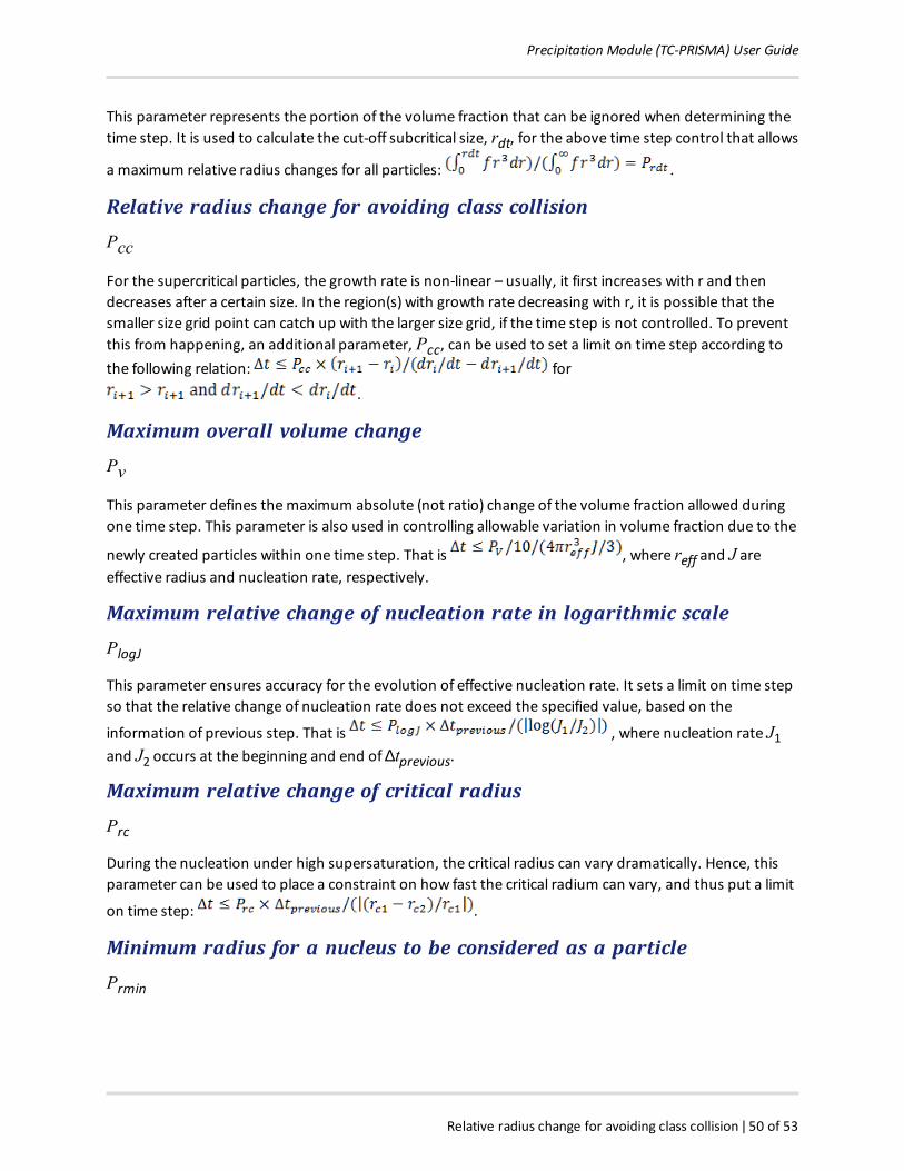
This parameter represents the portion of the volume fraction that can be ignored when determining thetime step. It is used to calculate the cut-off subcritical size, rdt, for the above time step control that allows

a maximum relative radius changes for all particles: .

Relative radius change for avoiding class collisionPcc

For the supercritical particles, the growth rate is non-linear – usually, it first increases with r and thendecreases after a certain size. In the region(s) with growth rate decreasing with r, it is possible that thesmaller size grid point can catch up with the larger size grid, if the time step is not controlled. To preventthis from happening, an additional parameter, Pcc, can be used to set a limit on time step according tothe following relation: for

.

Maximum overall volume changePv

This parameter defines themaximum absolute (not ratio) change of the volume fraction allowed duringone time step. This parameter is also used in controlling allowable variation in volume fraction due to the

newly created particles within one time step. That is , where reff and J areeffective radius and nucleation rate, respectively.

Maximum relative change of nucleation rate in logarithmic scalePlogJ

This parameter ensures accuracy for the evolution of effective nucleation rate. It sets a limit on time stepso that the relative change of nucleation rate does not exceed the specified value, based on the

information of previous step. That is , where nucleation rate J1and J2 occurs at the beginning and end of∆tprevious.

Maximum relative change of critical radiusPrc

During the nucleation under high supersaturation, the critical radius can vary dramatically. Hence, thisparameter can be used to place a constraint on how fast the critical radium can vary, and thus put a limit

on time step: .

Minimum radius for a nucleus to be considered as a particlePrmin


Maximum time step during heating stages ǀ 51 of 53

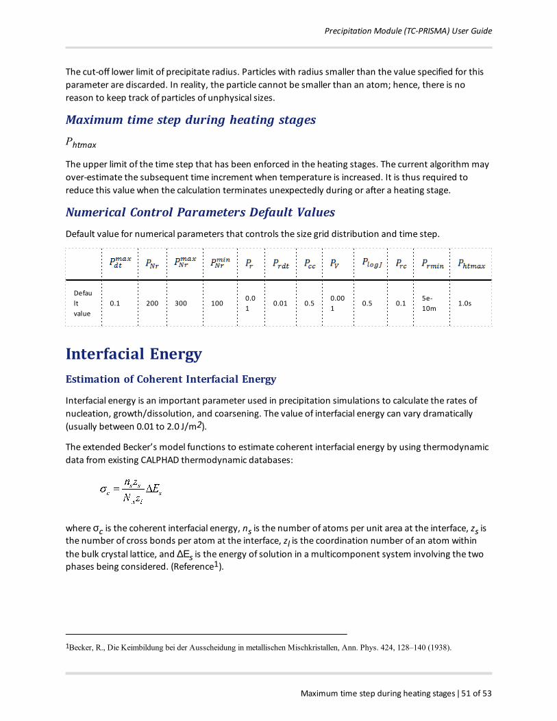
The cut-off lower limit of precipitate radius. Particles with radius smaller than the value specified for thisparameter are discarded. In reality, the particle cannot be smaller than an atom; hence, there is noreason to keep track of particles of unphysical sizes.

Maximum time step during heating stagesPhtmax

The upper limit of the time step that has been enforced in the heating stages. The current algorithm mayover-estimate the subsequent time increment when temperature is increased. It is thus required toreduce this value when the calculation terminates unexpectedly during or after a heating stage.

Numerical Control Parameters Default ValuesDefault value for numerical parameters that controls the size grid distribution and time step.

Defaultvalue

0.1 200 300 1000.01

0.01 0.50.001

0.5 0.15e-10m

1.0s

Interfacial EnergyEstimation of Coherent Interfacial Energy

Interfacial energy is an important parameter used in precipitation simulations to calculate the rates ofnucleation, growth/dissolution, and coarsening. The value of interfacial energy can vary dramatically(usually between 0.01 to 2.0 J/m2).

The extended Becker’s model functions to estimate coherent interfacial energy by using thermodynamicdata from existing CALPHAD thermodynamic databases:

where σc is the coherent interfacial energy, ns is the number of atoms per unit area at the interface, zs isthe number of cross bonds per atom at the interface, zl is the coordination number of an atom withinthe bulk crystal lattice, and ∆Εs is the energy of solution in a multicomponent system involving the twophases being considered. (Reference1).

1Becker, R., Die Keimbildung bei der Ausscheidung in metallischen Mischkristallen, Ann. Phys. 424, 128–140 (1938).


Precipitation Module (TC-PRISMA) References ǀ 52 of 53

Precipitation Module (TC-PRISMA) References1. Kampmann, R., and Wagner, R. (1991). "Homogeneous second phase precipitation". In

R. W. Cahn, P. Haasen, & E. J. Kramer (Eds.), Materials Science and Technology (pp.213–304). Weinheim, Germany: Wiley-VCH Verlag GmbH & Co. KGaA.

2. Langer, J. S., and Schwartz, A. J. (1980). "Kinetics of nucleation in near-critical fluids, "Physical Review A, 21(3), 948–958.

3. Kashchiev, D. (2000). Nucleation. Butterworth-Heinemann.

4. Svoboda, J., Fischer, F. D., Fratzl, P., and Kozeschnik, E. (2004). "Modelling of kinetics inmulti-component multi-phase systems with spherical precipitates, "Materials Scienceand Engineering: A, 385(1–2), 166–174.

5. Feder, J., Russell, K. C., Lothe, J., and Pound, G. M. (1966). "Homogeneous nucleationand growth of droplets in vapours, " Advances in Physics, 15(57), 111–178.

6. Cahn, J. W. (1956). "Transformation kinetics during continuous cooling", Acta Metal-lurgica, 4(6), 572–575.

7. Jou, H.-J., Voorhees, P., & Olson, G. B. (2004). "Computer simulations for the predictionof microstructure/property variation in aeroturbine disks", Superalloys, 877–886.

8. Chen, Q., Jeppsson, J., and Ågren, J. (2008). "Analytical treatment of diffusion during pre-cipitate growth in multicomponent systems," Acta Materialia, 56(8), 1890–1896.

9. Chen, M. K., and Voorhees, P. W. (1993). "The dynamics of transient Ostwald ripening",Modelling and Simulation in Materials Science and Engineering, 1(5), 591–612.

10. Aaron, H. B. (1970). "Diffusion-Limited Phase Transformations: A Comparison and Crit-ical Evaluation of the Mathematical Approximations", Journal of Applied Physics, 41(11),4404.

11. Becker, R. (1938). "Die Keimbildung bei der Ausscheidung in metallischen Mis-chkristallen", Annalen der Physik, 424(1–2), 128–140.

12. Wert, C. A. (1949). "Precipitation from Solid Solutions of C and N in α-Iron", Journal ofApplied Physics, 20(10), 943.

13. Clemm, P. , & Fisher, J. (1955). "The influence of grain boundaries on the nucleation ofsecondary phases", Acta Metallurgica, 3(1), 70–73.

14. Zang, L. (2004). Lecture 13: Heterogeneous Nucleation: Effects of Grain Boundaries andSurface Defects. Lecture slides, Salt Lake City, Utah: The Zang Research Group, TheUniversity of Utah. Retrieved from http://www.eng.utah.edu/~lzang/images/lecture-13.pdf


Precipitation Module (TC-PRISMA) References ǀ 53 of 53

15. Chen, Q., Wu, K., Sterner, G., and Mason, P. (2014). “Modeling precipitation kinetics dur-ing heat treatment with CALPHAD-based tools”, J. Mater. Eng. Perform., 23(12), 4193-4196.

16. Hou, Z., Hedström, P., Chen, Q., Xu, Y., Wu, D., and Odqvist, J. (2016). ”Quantitative mod-eling and experimental verfication of carbide precipitation in a martensitic Fe-0.16wt%C-4.0 wt%Cr alloy”, CALPHAD, 53( 6), 39-48.

precipitationmodule(tc-prisma)userguide … · contents introductiontotheprecipitation...

Documents