pre launch guidelines 3g
TRANSCRIPT

PRE LAUNCH GUIDELINES
Axel Abraham Valdes Vargas
1
PRE LAUNCH GUIDELINES

PRE LAUNCH GUIDELINES
Axel Abraham Valdes Vargas
2
Contents 1. Introduction ............................................................................................... 4
1.1.Purpose & Scope .................................................................................... 4
1.2.Definitions for this Document ................................................................ 4
2. UMTS technology in brief ......................................................................... 6
2.1.Architecture ............................................................................................. 7
2.2.UTRAN Interfaces .................................................................................... 8
3. Phases of Network Optimization .............................................................. 9
3.1.Objective .................................................................................................. 9
3.2.Optimization / Acceptance Phases ........................................................ 9
4.Cluster Optimization .................................................................................. 9
4.1.Objective ................................................................................................ 10
4.2. Process Flow ........................................................................................ 10
4.2.1. Cluster Unloaded Optimization ........................................................ 10
4.3.Actix Spotlight Post Processing .......................................................... 13
4.3.1.ACTIX Spotlight – Setup & Loading Log files................................... 14
4.3.1.1.Creating a Project Template ........................................................... 14
4.3.1.2.Creating a Spotlight Project ........................................................... 17
4.4. Log Files Analysis ................................................................................ 21
4.4.1.Swap Sector and SC Inconsistency Check Analysis ....................... 22
4.4.2.Azimuth Verification ........................................................................... 25
4.4.3.Sector Coverage / Boomer Cell Analysis.......................................... 26
4.4.4.Coverage Analysis ............................................................................. 26
4.4.4.1.RSCP – DL Coverage Optimization ................................................ 27
4.4.4.2.Ec/No – Pilot Dominance Optimization .......................................... 29
4.4.4.3. UE Transmit Power – UL Coverage ............................................... 33
4.4.4.4.Downlink BLER – Quality ................................................................ 34
4.4.4.5.Coverage Analysis – Deliverables.................................................. 35
4.4.5.Pilot Pollution Analysis ...................................................................... 35
4.4.5.1.Spotlight Cell Pollution Analysis .................................................... 35
4.4.5.2.Identifying Polluting Cells .............................................................. 38
4.5.Over-Propagating Cell Identification.................................................... 39
4.5.1.Spotlight Boomer Cell Analysis ........................................................ 39
4.5.2.Identifying Over-Propagating Cells ................................................... 40
4.6.UMTS Neighbor List Analysis............................................................... 41
4.6.1. Missing Neighbor Analysis ............................................................... 43
4.6.2.SHO Overhead Analysis .................................................................... 45

PRE LAUNCH GUIDELINES
Axel Abraham Valdes Vargas
3
4.7.Access Failure Analysis ....................................................................... 47
4.7.1.Spotlight Access Failure Analysis .................................................... 49
4.7.2.Access Failure Causes ...................................................................... 52
4.7.2.1 Which covers Missing Neighbor Analysis has additional detailed information which should be followed for neighbor analysis. ........ 54
4.7.2.2.RACH Access Troubleshooting ..................................................... 55
4.7.2.3. RRC Setup Troubleshooting .......................................................... 58
4.8.Drop Call Analysis................................................................................. 61
4.8.1.Drop Call Causes ................................................................................ 62
4.8.2. Drop Call Analysis in Spotlight ........................................................ 66
4.9. Packet Session Data Analysis ............................................................. 68
4.9.1. R99 DCH Low Throughput Analysis ................................................ 69
4.9.2.Using Actix To Identify Low R99 Throughput .................................. 70
4.9.3.Using Actix To Analyze Low R99 Throughput ................................. 74
4.9.4. HSDPA Low Throughput Analysis ................................................... 79
4.9.5.Using Actix To Identify Low HSDPA Throughput ............................ 80
4.9.5.1.Event Explorer ................................................................................. 80
4.9.5.2. Drill Down ....................................................................................... 81
4.9.5.3.Additional Attributes ....................................................................... 83
4.9.6. Using Actix To Analyze Low HSDPA Throughput ........................... 87
5. Market Level Optimization ...................................................................... 92
5.1.Objective ................................................................................................ 93
5.2.Process Flow ......................................................................................... 93
5.2.1.Market Loaded Optimization.............................................................. 93
5.3.IRAT Handover Failure Analysis .......................................................... 95
5.3.1.Identifying IRAT Handover Failures: ................................................. 95
5.3.2.IRAT Handover Failure Trouble Shooting Process .......................... 96
5.3.3. Global IRAT handover failures: ........................................................ 97
5.3.3.1.IRAT prerequisites: ......................................................................... 98
5.3.4. Cell Specific IRAT failures ................................................................ 98
5.3.4.1 Preparation Phase Failure ............................................................ 100
5.3.4.2. Execution phase failures. ............................................................ 102
5.3.4.3.Confirmation phase failures ......................................................... 105
PRE LAUNCH GUIDELINES
Axel Abraham Valdes Vargas
4
1. Introduction
1.1.Purpose & Scope
The purpose of this document is to provide guidelines for UMTS Pre-Launch Optimization in order to help the RF Optimization Engineers successfully optimize the KPI requirements for Cluster & SSV (Single Site Verification) Level Acceptance. Pre-launch optimization deals with assessing a newly-built network, uncovering problems and resolving them prior to the Launch phase. It entails detailed field RF measurements, detecting and rectifying problems caused by radio, improper parameter settings or network faults and finally, grading the radio access part of the network to make sure that it passes certain evaluation criteria.
This document is primarily focused on resolving typical RF issues through the Actix Spotlight platform. These guidelines will be revised to update Actix processing once ActixOne becomes available. In addition, whilst this document contains a lot of generic content, there is also content which is specific to Ericsson markets such as PM counters / parameters. Content specific to Nokia markets will be added at a later stage. At the pre-launch Optimization stage, it is not envisioned that large scale parameter changes will be necessary as primary actions such as Physical changes & some basic parameter changes only will be made. Hence, do not use this guidelines to change any parameters without there being satisfactory understanding of the consequences involved or unless there is an FSC mandate to do so.
1.2.Definitions for this Document
Term or Acronym Definition
3GPP Third Generation Partnership Project
AS Active Set
BSIC Base Station Identity Code
BTS Base Transceiver Station
CN Core Network
CPICH Common Pilot Channel
DCH Dedicated Channel
DL DownLink
DPCCH Dedicated Physical Control Channel

PRE LAUNCH GUIDELINES
Axel Abraham Valdes Vargas
5
DPCH Dedicated Physical Channel
DRNC Drift Radio Network Controller
FACH Forward Access Channel
FIFO First In First Out
GRAN GSM EDGE RAN
GSM Global System for Mobile Communications
HCS Hierarchical Cell Structure
IAF Intra Frequency
IE Information Element
IEF Inter Frequency
IFHO Inter Frequency HandOver
Inter-RAT Inter Radio Access Technology
IRAT Inter Radio Access Technology
Iur Interface between two RNCs
KPI Key Parameter Indicator
LA Location Area
LAI Location Area Indicator
NBAP Node B Application Part
Node B Logical node responsible for radio transmission and reception in one or several cells
OCNS Orthogonal Channel Noise Simulator
PLMN Public Land Mobile Network
RA Routing Area
RAB Radio Access Bearer
PRE LAUNCH GUIDELINES
Axel Abraham Valdes Vargas
6
RAI Routing Area Indicator
RAN Radio Access Network
RAT Radio Access Technology
RB Radio Bearer
RBS Radio Base Station – another name for the Node B
RF Radio Frequency
RL Radio Link
RNC Radio Network Controller
RRC Radio Resource Control
RSCP Received Signal Code Power
RSSI Received Signal Strength Indicator
SIB System Information Block
SIR Signal to Interference Ratio
TRX Transceiver
TX Transmit
UE User Equipment
UL UpLink
UMTS Universal Mobile Telecommunication Services
UTRAN UMTS Terrestrial Radio Access Network
WCDMA Wideband Code Division Multiple Access
2. UMTS technology in brief
Wideband CDMA is the recognized air interface standard for 3G-UMTS. It was developed as one of the third generation radio access technologies whose ultimate goal is better spectrum efficiency, faster data transfer rate and an increase in service quality.
PRE LAUNCH GUIDELINES
Axel Abraham Valdes Vargas
7
WCDMA utilizes the spread spectrum technology for radio access where users are identified by unique codes, which means that all users can use the same frequency and transmit at the same time. A bandwidth of 5MHz is used per channel with a chip rate of 3.84 Mcps.
For optimal operation of the wireless system, several functions are in place to control the radio network and the many active handsets. Efficient power control in both directions regulates the over-all interference level which is very important in a network with a frequency reuse of 1. Fast power control algorithms at 1500 Hz counter fading dips and ensure good performance. “Cell breathing” is a phenomenon inherent in WCDMA. This is the trade-off between coverage and capacity where the size of the cell varies depending on the current load. Macro diversity is another feature of the network which is achieved during soft handover. A user can be connected to two or three base stations at a time providing a more reliable connection, thus reducing the risk of premature disconnection. A drawback with soft handover is that it requires additional hardware resources on the network side, as the handset has multiple connections. In a well-designed radio network, 30–40 % of the users will be in soft or softer handover. Other system functionalities are admission and congestion controls which, as the names imply, are responsible for maintaining optimum loading in all parts of the radio network. Some of the ways by which this is done are by selective admission of users depending upon the expected noise level contribution and by dynamic reduction of the bitrates of certain non-real time applications to resolve overload situations.
2.1.Architecture
For mobile network operators normally has an existing GSM infrastructure, the migration scheme towards 3G primarily involves annexing a UMTS Terrestrial Radio Access Network (UTRAN) to the current setup. Both the GSM BSS and the UTRAN are connected to the same core network which handles all voice and data traffic from both systems, in circuit-switched (CS) or packet-switched (PS) modes.
The UTRAN which is analogous to the BSS in GSM consists of the Radio Network Controller (RNC) and the linked Node Bs which basically has similar functionalities as the BSC and BTS, respectively.

PRE LAUNCH GUIDELINES
Axel Abraham Valdes Vargas
8
Figure 1: GSM/UMTS Network Architecture & interfaces
2.2.UTRAN Interfaces
With the advent of new UMTS standards, comes a new set of interfaces and hence, interface names. Within the UTRAN, the main interfaces are:
• Iu – an open, multi-vendor interface that connects the UTRAN to the core network. It can have two different physical instances, the Iu-CS and Iu-PS, respectively connecting circuit switched and packet switched traffic into the core network, equivalent to the A and Gb interfaces in GSM
• Iur – connects two RNC’s belonging to the same PLMN, supporting exchange of both signaling and user data. Non-existent between BSCs in GSM, this interface is there to support macrodiversity in UMTS. During soft-handover situations when a user equipment (UE) is connected to two or more Node Bs that belong to different RNC’s, the Iur makes it possible for the controlling RNC to manage the process by itself. In cases where the Iur does not support user plane transfer or if this link is not in place at all, this control is handled via the Iu interface through the MSC. The process now becomes the so-called hard handover.
• Iub – situated between the RNC and the Node B, performing rather complex tasks between the two entities. The interface protocols are fully specified by 3GPP making it possible to link Node Bs and RNC’s from different compliant vendors. In GSM, this interface is the Abis.
• Uu – the air interface between the base stations and the UE
Although the Uu interface is obviously where RF optimization will be focused most of the time, an understanding of the functionality aspect of the other interfaces is vital to being able to make a well-rounded approach to problem solving and fault isolation.

PRE LAUNCH GUIDELINES
Axel Abraham Valdes Vargas
9
3. Phases of Network Optimization
3.1.Objective
In a nutshell, the main goal of pre-launch optimization is to make the UMTS network ready for the Launch Phase. To achieve this, a series of tests and tuning methods must be carried out and repeated as many times as required in order to meet certain performance criteria. Tests will basically start from cell level and then progressively widen in scope to encompass larger groups of cells until the entire market is tested as one functioning unit.
3.2.Optimization / Acceptance Phases
In preparing for launch, the network undergoes various phases as shown in the diagram below.
Figure 2: Optimization Process
This document details the phases starting from Cluster Unloaded Optimization through to Market Launch. All other phases are outside the scope of this document and are covered in other literature.
4.Cluster Optimization
To perform Cluster Level Optimization, a Market is divided into several clusters. Each cluster contains about 60-90 sites depending on the site density, morphology and expected subscriber’s mobility. There will be a team of one RF Engineer and one Drive Testing Engineer responsible for a Cluster to complete the Cluster Level Optimization. Each cluster can be broken down in mini sub-clusters to ease the drive testing process. However, the final KPIs are computed from this 60-90 site cluster.
PRE LAUNCH GUIDELINES
Axel Abraham Valdes Vargas
10
4.1.Objective
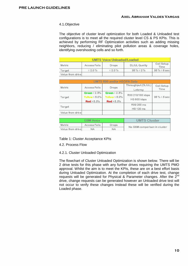
The objective of cluster level optimization for both Loaded & Unloaded test configurations is to meet all the required cluster level CS & PS KPIs. This is achieved by performing RF Optimization activities such as adding missing neighbors, reducing / eliminating pilot pollution areas & coverage holes, identifying overshooting cells and so forth.
Table 1: Cluster Acceptance KPIs
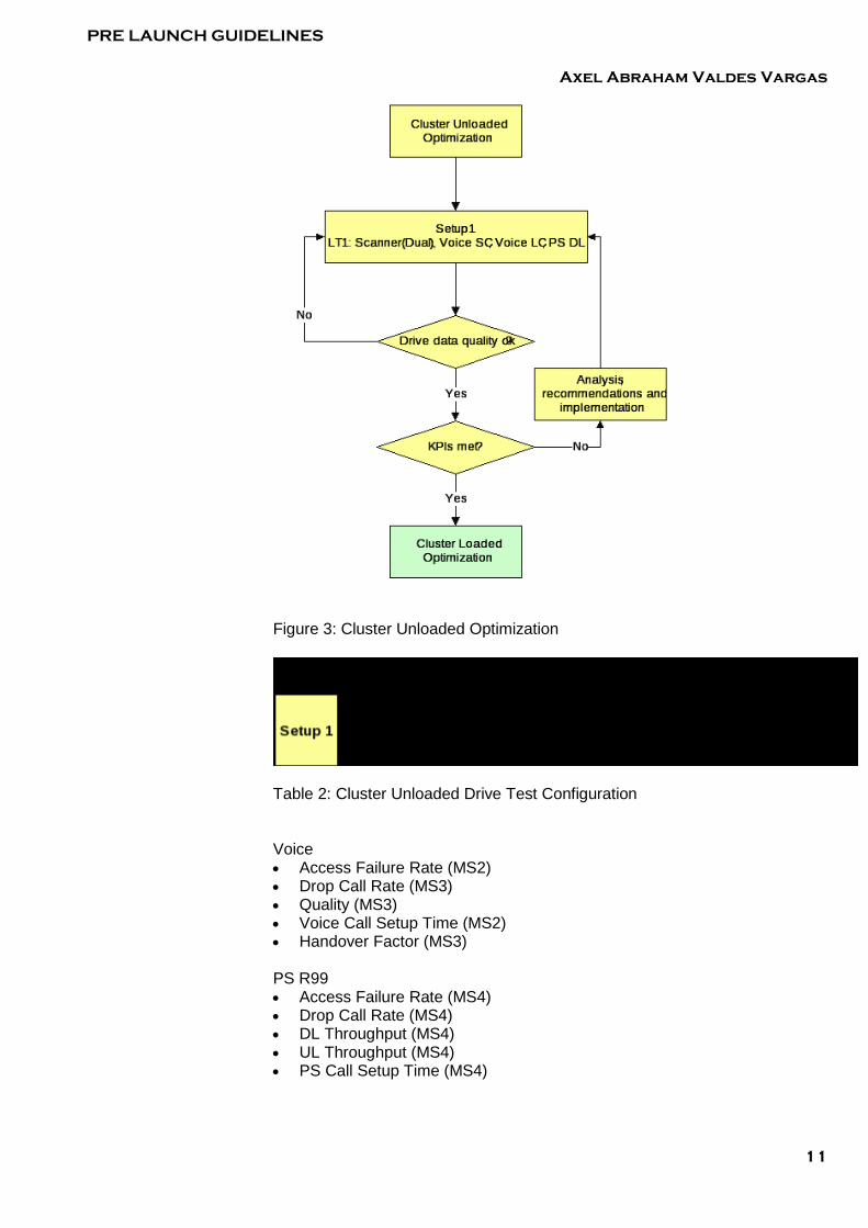
4.2. Process Flow 4.2.1. Cluster Unloaded Optimization The flowchart of Cluster Unloaded Optimization is shown below. There will be 2 drive tests for this phase with any further drives requiring the UMTS PMO approval. Whilst the aim is to meet the KPIs, these are on a best effort basis during Unloaded Optimization. At the completion of each drive test, change requests will be generated for Physical & Parameter changes. After the 2nd drive, change requests can be generated however an Unloaded drive test will not occur to verify these changes Instead these will be verified during the Loaded phase.
PRE LAUNCH GUIDELINES
Axel Abraham Valdes Vargas
11
Figure 3: Cluster Unloaded Optimization
Table 2: Cluster Unloaded Drive Test Configuration Voice • Access Failure Rate (MS2) • Drop Call Rate (MS3) • Quality (MS3) • Voice Call Setup Time (MS2) • Handover Factor (MS3) PS R99 • Access Failure Rate (MS4) • Drop Call Rate (MS4) • DL Throughput (MS4) • UL Throughput (MS4) • PS Call Setup Time (MS4)
PRE LAUNCH GUIDELINES
Axel Abraham Valdes Vargas
12
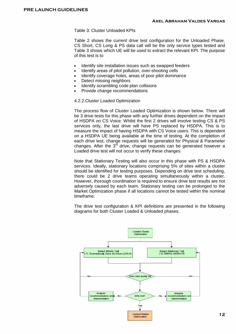
Table 3: Cluster Unloaded KPIs Table 2 shows the current drive test configuration for the Unloaded Phase. CS Short, CS Long & PS data call will be the only service types tested and Table 3 shows which UE will be used to extract the relevant KPI. The purpose of this test is to • Identify site installation issues such as swapped feeders • Identify areas of pilot pollution, over-shooting cells • Identify coverage holes, areas of poor pilot dominance • Detect missing neighbors • Identify scrambling code plan collisions • Provide change recommendations 4.2.2.Cluster Loaded Optimization The process flow of Cluster Loaded Optimization is shown below. There will be 3 drive tests for this phase with any further drives dependent on the impact of HSDPA on CS Voice. Whilst the first 2 drives will involve testing CS & PS services only, the last drive will have PS replaced by HSDPA. This is to measure the impact of having HSDPA with CS Voice users. This is dependent on a HSDPA UE being available at the time of testing. At the completion of each drive test, change requests will be generated for Physical & Parameter changes. After the 3rd drive, change requests can be generated however a Loaded drive test will not occur to verify these changes. Note that Stationary Testing will also occur in this phase with PS & HSDPA services. Ideally, stationary locations comprising 5% of sites within a cluster should be identified for testing purposes. Depending on drive test scheduling, there could be 2 drive teams operating simultaneously within a cluster. However, thorough coordination is required to ensure drive test results are not adversely caused by each team. Stationary testing can be prolonged to the Market Optimization phase if all locations cannot be tested within the nominal timeframe. The drive test configuration & KPI definitions are presented in the following diagrams for both Cluster Loaded & Unloaded phases.

PRE LAUNCH GUIDELINES
Axel Abraham Valdes Vargas
13
Figure 4: Cluster Loaded Optimization
Table 5: Cluster Loaded KPIs – Mobile Test The purpose of this test is to: • Validate the RF Design criteria such as Ec/No & RSCP against the actual
network performance • Identify areas of pilot pollution, over-shooting cells • Identify coverage holes, areas of poor pilot dominance • Provide change recommendations • Investigate any significant KPI degradations experienced by CS Voice
UEs when a HSDPA UE is present • Provide change recommendations
Figure 5: Cluster Loaded KPIs – Stationary Test The purpose of this test is to: • Identify the peak & mean throughputs for PS R99 services • Identify the latency times for PS R99 services • Identify the peak & mean throughputs for HSDPA • Identify the latency times for HSDPA • Investigate areas of non-existent 16-QAM when it should exist • Provide change recommendations Whilst the drive test configurations & KPIs have been shown above, this document will not provide details regarding how to perform drive tests. All detailed content relating to Drive Test Setup. 4.3.Actix Spotlight Post Processing

PRE LAUNCH GUIDELINES
Axel Abraham Valdes Vargas
14
This section discusses Post Processing of TEMS Log files to identify the areas of Optimization in the UMTS Radio Network. Actix Spotlight is the tool for post processing the TEMS Log files. When this document was written, the ActixOne platform was not in place. Hence in this document, the process assumes every Cluster RF Engineer has a Standalone Desktop loaded with Actix Spotlight. 4.3.1.ACTIX Spotlight – Setup & Loading Log files The purpose of this section is to describe the procedure for creating a Spotlight project with Actix Analyzer Software. Spotlight, allows the user to use automated workflow and analysis to investigate, troubleshoot, and report UMTS and HSDPA drive data. Suitable for large data volumes, it creates a dashboard that highlights certain event types and allows a user to drill down in a specific file without loading it in its entirety. The following subjects will be discussed in this section: • Creating a Project Template in Actix Spotlight • Creating a Project in Actix Spotlight and Loading log files • Handling Projects • Various Actix Spotlight features
With ActixOne in place, it will not be required to do many of the steps in this section. For example, it will not be required to create a project/template, Celref, etc. It will not be required to load the log files. A project will already exist in ActixOne for a specific cluster and this can be worked on immediately. 4.3.1.1.Creating a Project Template When Actix is initially opened, the user will be provided the option to open Actix Classic or Actix Spotlight. Choose the option that allows the user to open Actix Spotlight when the following screen appears, Figure 6.
Figure 6: Choosing An Engineering Process

PRE LAUNCH GUIDELINES
Axel Abraham Valdes Vargas
15
After choosing Actix Spotlight, the following screen will appear as shown in Figure 7. All previously created projects will be visible as well as the ability to create a new one. Hence, select the New Project button.
Figure 7: Creating A New Project Spotlight comes standard with several templates available. In addition, a user can create a new template using an existing one as a base. The following procedure describes the process of creating a new Template. Select the New Template button as shown in Figure 8.
Figure 9: Creating A New Project Template The New Project Template Step 1 screen gives the user a chance to create a name for the new template and to select an existing template to base it on. Type in a new name in the Template Name field, and select UMTS Voice from the drop-down menu. Note that other templates are to start from if appropriate (e.g. GSM UMTS Voice) if required. This procedure assumes only UMTS data is being processed. Once finished, click the Next button as shown in Figure 9.
Figure 9: Naming The New Project Template

PRE LAUNCH GUIDELINES
Axel Abraham Valdes Vargas
16
After creating a name for the new template, Step 2 allows the devices that will be processed to be selected. This option allows the user to define which devices will be loaded for the Spotlight analysis. For example, if the user is only interested in analyzing scanner data, and excluding all other devices, this could be achieved by clicking the Add Device button and creating the appropriate filter. This may be useful in reducing the processing time if the log files contain data from multiple devices. The default setting is All devices and is generally recommended to insure that all data is loaded. After creating the appropriate filter click the Next button.
Figure 10: Select Devices For Template The next step is to define the KPIs that will be analyzed, and the Reports that will be created. Based on these selections, Spotlight will create a dashboard that reports on different types of events. To investigate the full range of UMTS/HSDPA failures, ensure that the checkboxes are selected as shown in Figure 11. After making the appropriate selections, click the Next button.
Figure 11: Selecting KPIs And Reports Now that the various KPIs have been chosen, Step 4 allows Attributes to be added (see Figure 13). The base template that was selected comes with several Binned Data Queries that include default attributes. These attributes will be available for viewing in Spotlight’s “dashboard”. In addition, other attributes of interest can be added. For example, to add the Average HSDPA CQI attribute, select the UMTS UE Binned Data query to list the currently selected attributes. Next, select the attribute from the Attribute Picker (i.e. 3G UMTS > Downlink Measurements > 3G HSDPA > Uu_HSDPA_CQI_Average).

PRE LAUNCH GUIDELINES
Axel Abraham Valdes Vargas
17
Figure 12: Adding An Attribute To A Binned Query Included in Step 4 is the data binning options which is illustrated in Figure 13. Typically, area binning will be used when Pilot Pollution and Neighbor List analysis is required. Select the meters radio button as the Units of Measurement, and enter the X and Y bin size. The bin size utilized should be based on the binning that was used by Asset 3G during the design phase. For example, if 5 meter bins were used for the Manhattan design, then the same bin size should be used for the Spotlight analysis. Finally, select Conformal Project (USA) from the Projection drop down box, and click the Next button.
Figure 13: Binning Options The final step in the process is to define Global Filters. This is typically left unchanged. Complete the template creation process by selecting the Done button as shown in Figure 14.
Figure 14: Template Completion 4.3.1.2.Creating a Spotlight Project
PRE LAUNCH GUIDELINES
Axel Abraham Valdes Vargas
18
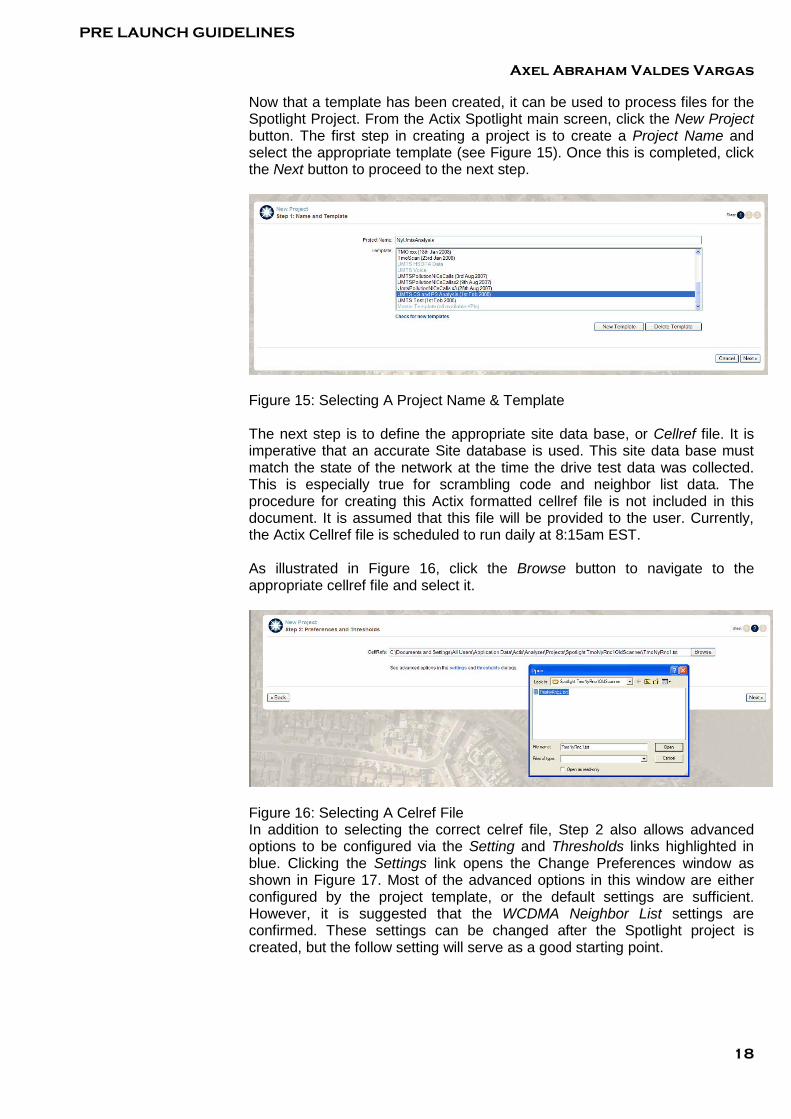
Now that a template has been created, it can be used to process files for the Spotlight Project. From the Actix Spotlight main screen, click the New Project button. The first step in creating a project is to create a Project Name and select the appropriate template (see Figure 15). Once this is completed, click the Next button to proceed to the next step.
Figure 15: Selecting A Project Name & Template The next step is to define the appropriate site data base, or Cellref file. It is imperative that an accurate Site database is used. This site data base must match the state of the network at the time the drive test data was collected. This is especially true for scrambling code and neighbor list data. The procedure for creating this Actix formatted cellref file is not included in this document. It is assumed that this file will be provided to the user. Currently, the Actix Cellref file is scheduled to run daily at 8:15am EST. As illustrated in Figure 16, click the Browse button to navigate to the appropriate cellref file and select it.
Figure 16: Selecting A Celref File In addition to selecting the correct celref file, Step 2 also allows advanced options to be configured via the Setting and Thresholds links highlighted in blue. Clicking the Settings link opens the Change Preferences window as shown in Figure 17. Most of the advanced options in this window are either configured by the project template, or the default settings are sufficient. However, it is suggested that the WCDMA Neighbor List settings are confirmed. These settings can be changed after the Spotlight project is created, but the follow setting will serve as a good starting point.

PRE LAUNCH GUIDELINES
Axel Abraham Valdes Vargas
19
Figure 17: Change Preferences At this point, click the Thresholds link to open the Thresholds Editor (see Figure 18). In most cases, default setting will be appropriate (defaults can be restored by clicking the Restore Defaults button). However the Uu_CallSetupFailure_Num_RRCConnReq threshold (expand UMTS > Event Control) should be set to 5 to match the recommended value for the configurable RNC parameter N300. In addition, confirm that the threshold Uu_Scan_TooManyServersThreshold (expand UMTS > Scan_Coverage) is set to 5. Lastly, the SL_Overspill_Dist_Threshold (located in the Spotlight folder) should be adjusted based on the morphology and site density of the area to be analyzed. For example, Manhattan will require a lower value (e.g. 500 meters) while North Dallas may only require 2000 meters. This threshold will help identify over propagating (Boomer) cells. Alternatively, this threshold can be configured on a per cell basis by means of the cellRef file, which is the better option. Once the thresholds have be modified and confirmed, click the OK button to exit and save the threshold changes. At this point click the Next button to move to step 3.
Figure 18: Threshold Editor

PRE LAUNCH GUIDELINES
Axel Abraham Valdes Vargas
20
The final step is to select the files to be processed. Click the Add Files button as shown in Figure 19. Optionally, all files in a folder can be added by selecting the Add Folder button. Navigate to the appropriate folder, select the files or sub-folder, and click Open.
Figure 19: Adding Log Files After all files have been selected (see Figure 20), click the Done button to begin processing the selected log files. At this point, a status bar appears indicating the status of the data processing.
Figure 20: Selected Files After the log files have been loaded and processed, a Data Processing Summary window appears indicating how many files loaded, and how many files failed to load. In some cases, not all files initially load due to computer limitations (e.g. processing capability and limited memory). If files fail to load, reselect the files and attempt to load them again. If files fail to initially load, however successfully load on repeated attempts, consider reducing the amount of data loaded during each attempt. On the other hand, if a specific file continuously fails to load, it may be corrupt. Once the Data Processing Summary window is closed, the Spotlight Summary Dashboard appears (see Figure 21). At this point, additional log files can be loaded by clicking the Add Data link. Before proceeding with the analysis phase, confirm that all log files have been loaded. The Repository Summary indicates the number of log files loaded. This number should match the number of log files that were intended to be loaded (less any corrupt files).

PRE LAUNCH GUIDELINES
Axel Abraham Valdes Vargas
21
Figure 21: Spotlight Summary Dashboard 4.4. Log Files Analysis The objective of analyzing Log files is to make the network meet the required Cluster Level KPIs (as per Table 1) by identifying issues and resolving it through optimization. Following are the metrics that a Cluster RF Engineer may consider for analysis in general. • Coverage plot in terms of RSCP – To identify the areas of poor coverage • Best Server Plot (1st Best SC based on Ec/No) – To verify the sector wise
coverage, SC inconsistencies, Sector Swaps, etc. • Ec/No Plot of the 1st Best Server – To identify areas of poor Ec/No • Downlink BLER plot – To identify the areas of poor down link quality • UE Transmit Power Plot – To identify the areas of poor uplink coverage
and path imbalance • Uplink BLER – To identify the areas of poor uplink quality ( Possible only
with UETR Trace files) • Active Set Size Plot – To identify the areas of high secondary traffic and
too many servers. Following is the analysis that a Cluster RF Engineer may need to exercise to identify issues and reach optimization solutions. • Swap Sector Analysis / SC inconsistency Check – To identify the sector
swaps and/or improper data fill of Scrambling codes • Azimuth Verification – To identify the difference between the azimuth
deployed and azimuth designed. • Missing Neighbor Analysis – To identify the reported missing neighbors
and recommend the required neighbor list changes. • Analysis of Pilot Pollution / Interference / Pilot Overshoot – To identify the
possible cause of poor Ec/No, poor DL BLER, High SHO overhead, etc. • Drop Calls / Access Failure Analysis – To identify the reason for Drop
calls and Access Failures and provide to solutions to resolve.
PRE LAUNCH GUIDELINES
Axel Abraham Valdes Vargas
22
Following are the analysis that a RNC Engineer may need to do on a RNC Level for all the sites. • Neighbor List Inconsistency Check – To identify issues like one way
neighbors, neighbor data fill issues, IRAT Neighbor issues, etc. • SC Inconsistency Check – To identify any SC collisions based on
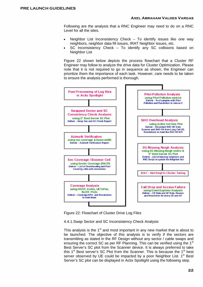
Neighbor List Figure 22 shown below depicts the process flowchart that a Cluster RF Engineer may follow to analyze the drive data for Cluster Optimization. Please note that it is not required to go in sequence as shown, the Engineer can prioritize them the importance of each task. However, care needs to be taken to ensure the analysis performed is thorough.
Figure 22: Flowchart of Cluster Drive Log Files 4.4.1.Swap Sector and SC Inconsistency Check Analysis This analysis is the 1st and most important in any new market that is about to be launched. The objective of this analysis is to verify if the sectors are transmitting as stated in the RF Design without any sector / cable swaps and ensuring the correct SC as per RF Planning. This can be verified using the 1st Best Server’s SC plot from the Scanner device. It is always preferred to take this 1st Best server’s SC Plot from the Scanner. This is because the 1st best server observed by UE could be impacted by a poor Neighbor List. 1st Best Server’s SC plot can be displayed in Actix Spotlight using the following step.

PRE LAUNCH GUIDELINES
Axel Abraham Valdes Vargas
23
• In the Summary Dashboard, select the ‘Scanner’ tab • Click on the ‘Radio Network’ button which will take you to the Radio
Network Explorer window • Select the ‘Cell Coverage’ tab in Radio Network Explorer window • From the Attributes select ‘CPICH_Scan_SC_SortedbyEcIo_0’. This will
display the 1st Best Server’s SC in the Map window as shown below in Figure 23.
One should also make sure that the loaded ‘cellref’ file in Actix Spotlight has the updated SC, Azimuths, etc.
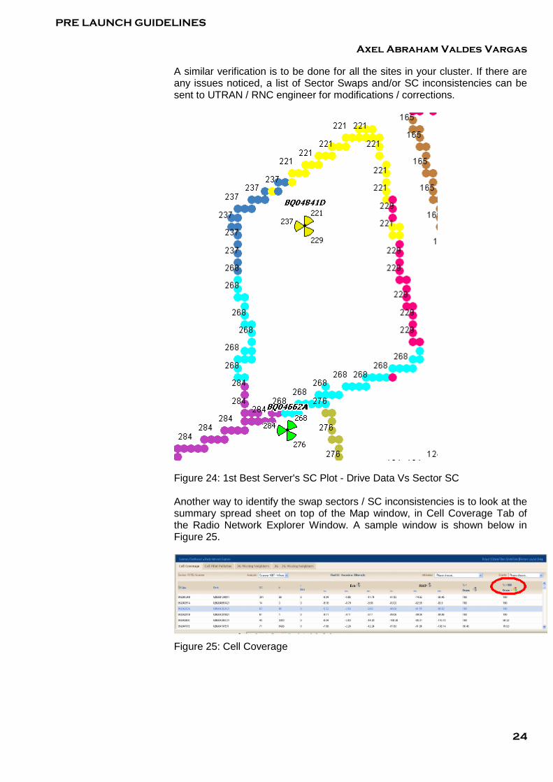
Figure 23: 1st Best Server SC Plot It is recommended to label the sectors and the drive map (using layer control in the map window) with SC. A visual verification over the plot would reveal that if there are any sectors swaps and/or SC inconsistencies. A zoomed picture of 1st Best Server’s SC plot is shown below. As we see here, the drive data’s SC exactly matches with the SC of the sectors. Incase, if there is a sector swap, we should see otherwise. For example in Figure 24 shown below, on site B104841D, if sectors 1 and 2 are swapped, then we should see SC 229 on top then 221 below. Sometimes, all the three sectors in a site would have been swapped. Say, Sec1 Sec 2, Sec2 Sec3 and Sec3 Sec1. This can also be identified in the SC Plot. Instead of 221, 229 & 237, you will see like 237, 221 and 229 (shifted clockwise). In few other cases, if the planned SC is not data filled properly in RNC / NodeB, you may see a different SC in drive data than the one in the site. This is known as a SC Inconsistency.
PRE LAUNCH GUIDELINES
Axel Abraham Valdes Vargas
24
A similar verification is to be done for all the sites in your cluster. If there are any issues noticed, a list of Sector Swaps and/or SC inconsistencies can be sent to UTRAN / RNC engineer for modifications / corrections.
Figure 24: 1st Best Server's SC Plot - Drive Data Vs Sector SC Another way to identify the swap sectors / SC inconsistencies is to look at the summary spread sheet on top of the Map window, in Cell Coverage Tab of the Radio Network Explorer Window. A sample window is shown below in Figure 25.
Figure 25: Cell Coverage
PRE LAUNCH GUIDELINES
Axel Abraham Valdes Vargas
25
This spread sheet the cell wise coverage statistics observed during the drive test. You can sort this spread sheet in terms of ‘% >180 Beam’, by clicking on it. This will bring up sites which are having most drive samples falling out side the imaginary antenna beam width. Higher the percentage in this column means more drive samples are falling out side the 180 deg imaginary antenna beam width. This could be an issue of Sector Swap and/or SC inconsistency. If you click on the particular site with high percentage, it will take you to that site on map window, displaying the RSCP of that sector. On this map window, by displaying the 1st Best Server’s SC, you will be able to analyze if there is any Sector Swap and/or SC Inconsistency as discussed above. Following are the cautions that should be considered in this analysis • Detailed drive data should be available to do this analysis. Hence, it is
recommended to do this analysis with the Cluster Tuning Drive but not with Market Drives
• This analysis should not be done for the sites at the edge of the cluster or drive area, especially for the sectors facing outside the cluster or drive area.
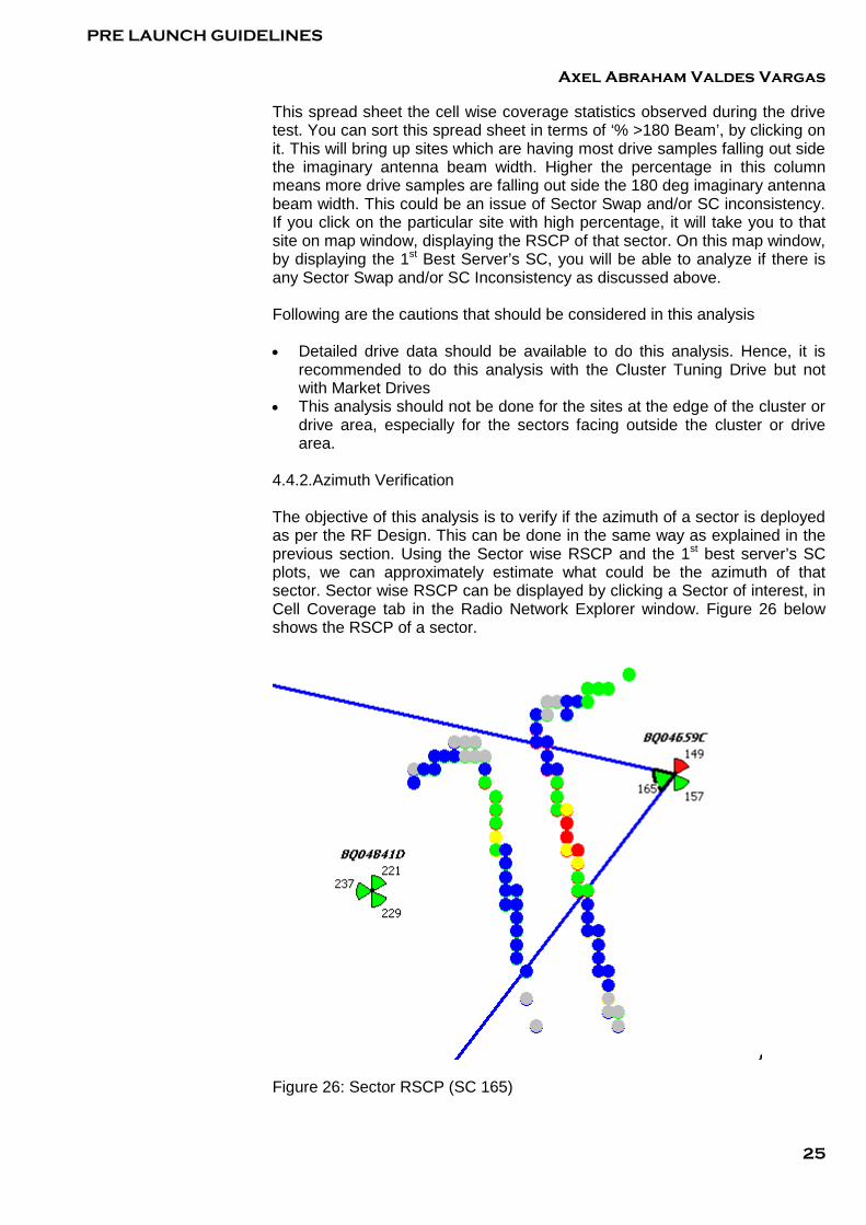
4.4.2.Azimuth Verification The objective of this analysis is to verify if the azimuth of a sector is deployed as per the RF Design. This can be done in the same way as explained in the previous section. Using the Sector wise RSCP and the 1st best server’s SC plots, we can approximately estimate what could be the azimuth of that sector. Sector wise RSCP can be displayed by clicking a Sector of interest, in Cell Coverage tab in the Radio Network Explorer window. Figure 26 below shows the RSCP of a sector.
Figure 26: Sector RSCP (SC 165)
PRE LAUNCH GUIDELINES
Axel Abraham Valdes Vargas
26
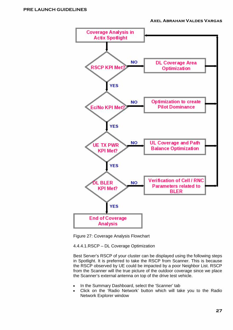
It should be noted that, in this analysis, we are not trying to estimate the azimuth accurately. It’s only an approximate estimation. If a difference in azimuth noticed, a cell technician need to be sent to the site for verification, before making any work order for change of azimuth. 4.4.3.Sector Coverage / Boomer Cell Analysis This analysis can be done in parallel with Azimuth Verification (4.4.24.4.2) Coverage of a Sector can be displayed by clicking on the Sector of interest on the Map window while in Cell Coverage Tab in Radio Network Explorer Window. It is recommended to choose the Scanner as the device to look at the Sector Coverage. Figure 26 shows an example of coverage in terms of RSCP of a sector. Generally a Sector Coverage in terms of RSCP should be better than -104 dBm up to the next near by neighbor cell. This will make sure there is enough coverage and big coverage holes in the cell edges. It is recommended to verify the coverage of every sector in your cluster in this way. In case if you find any site covering very low (very low coverage radius), then following could be the issues: • Improper Antenna Azimuth • Improper Electrical and/or Mechanical Tilt • Major Obstructions • Node B hardware issues • High VSWR on Feeder Cables • Poor RF Connectors / Antenna If a poor coverage is noticed from any of the sectors, please make a note of the sectors and validate these sectors while doing the cluster level detailed coverage analysis as per 4.4.4 In some cases, you find that the cell coverage exceeds beyond the 2nd or 3rd tier Cells. This could due to Overshooting pilots also known as Boomer Cells. Please refer to 4.5 about identifying the overshooting pilots and optimizing it. In few circumstances, because of the clutter type, a 2nd Tier Cell will be the strongest serving cell for the UE. This could be because of any major obstruction on the 1st Tier Cell. In this case, the 2nd Tier Cell should not be considered as an overshooting pilot or Boomer Cell. 4.4.4.Coverage Analysis Coverage Analysis would generally be the first step in Log files Analysis. The Objective of Coverage Analysis is to make sure that the coverage of a site or the cluster from the drive test meets the coverage objective of the RF Design. Figure 27 below shows the process that a Cluster RF Engineer may follow to perform coverage analysis.
PRE LAUNCH GUIDELINES
Axel Abraham Valdes Vargas
27
Figure 27: Coverage Analysis Flowchart 4.4.4.1.RSCP – DL Coverage Optimization Best Server’s RSCP of your cluster can be displayed using the following steps in Spotlight. It is preferred to take the RSCP from Scanner. This is because the RSCP observed by UE could be impacted by a poor Neighbor List. RSCP from the Scanner will the true picture of the outdoor coverage since we place the Scanner’s external antenna on top of the drive test vehicle. • In the Summary Dashboard, select the ‘Scanner’ tab • Click on the ‘Radio Network’ button which will take you to the Radio
Network Explorer window

PRE LAUNCH GUIDELINES
Axel Abraham Valdes Vargas
28
• Select the ‘Cell Coverage’ tab in Radio Network Explorer window • From the Attributes select ‘CPICH_Scan_RSCP_SortedbyEcIo_0’. This
will display the 1st Best Server’s RSCP in the Map window as shown below in Figure 28.
Figure 28: Spotlight RSCP Plot The objective of RSCP analysis is to meet the required RF Design KPI in terms of RSCP. This KPI would differ from market to markets. For example, in NY the RSCP should be better than -105 dBm at 100% of the area. To find out the Percentage of RSCP from drive test that is better than -105 dBm, please refer the Map Legend on the right side of Map window. You can calculate the percentage of samples above -105 dBm to the total number of drive test samples. If the KPI is not met, then a visual verification of plot would reveal the areas of coverage less than -105 dBm. An attempt should be made to improve DL coverage in those patches. Apart from meeting the RSCP KPI, it is also recommended to make a visual verification of drive test RSCP in comparison with the RSCP prediction from the RF Design. A sample of such comparison is shown in Figure 29 below. Where ever the drive test RSCP is inferior to the Predicted RSCP, an attempt should be made to do a DL Coverage Optimization.

PRE LAUNCH GUIDELINES
Axel Abraham Valdes Vargas
29
Figure 29: Drive Test RSCP Vs RF Design Predicted RSCP DL COVERAGE (RSCP) OPTIMIZATION The intention of DL Coverage Optimization is to improve the RSCP to a level as optimum as possible. It is always recommended to identify the 1st Best Server in terms of Ec/No, in the area you are optimizing. And then try improving the RSCP of that sector. Following could be the causes of poor coverage from a sector. • Obstructions – Buildings, Hoardings, etc. • Either very high or very low Electrical / Mechanical Tilts • Improper Antenna Azimuth • Improper Antenna • High Feeder Cable Loss due to higher feeder cable length • Feeder Cable / Connecter issues • Incorrect CPICH Power • Incorrect NodeB parameters like, ulAttenuation, dlAttenuation, TMA
insertion loss, etc. • Node B Hardware Issues, Alarms, etc. Following are the ways the Cluster RF Engineer may try to optimize the coverage. • Change of RET (No or Low Cost) • Change of Azimuths (High Cost) • Change of Mechanical Tilts (High Cost) • Change of Antenna (Very High Cost) • Verify the CPICH power from the RNC dump of the day of drive test • Verify if there was any Node B Alarm on the day of drive test • If the feeder cable or Node Hardware suspected, a cell tech may be sent
to the site to verify the feeder cable, connectors, VSWR, hardware issues, etc
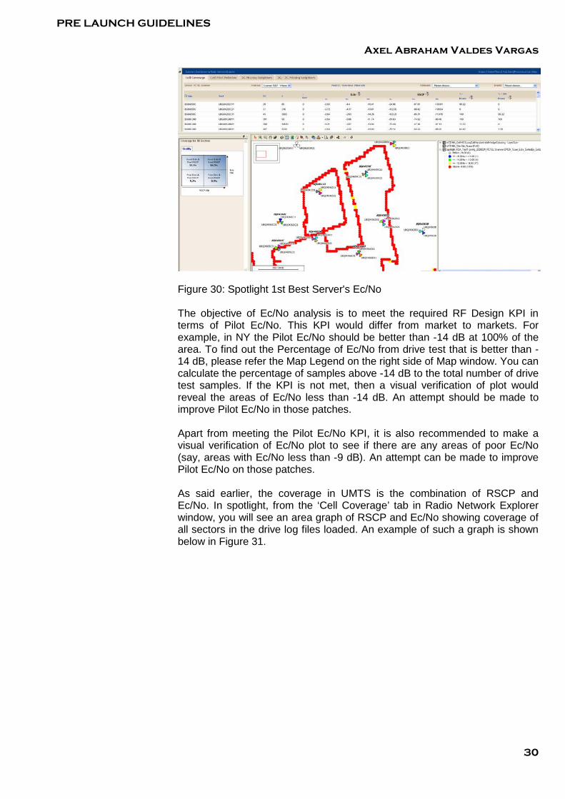
In case if it is not possible to optimize 1st Best Server’s Sector, or if the poor coverage patch is at the cell edges, then you can try to improve the coverage of the 2nd Best or 3rd Server’s Sector. But in this case, you should try to reduce coverage from 1st Best Server, so that your optimization does not lead to pilot pollution, poor Ec/No or higher soft handover overhead. 4.4.4.2.Ec/No – Pilot Dominance Optimization DL coverage in UMTS is not just the RSCP but the combination of RSCP and Ec/No. Care should be taken throughout the optimization, to create or keep a Pilot dominant in any given coverage area. Single or less number of pilots in an area leads to less ‘Io’ and hence better Ec/No. It is recommended to the Ec/No from the Scanner, because of the fact that Ec/No observed by UE could be impacted by a poor Neighbor List. 1st Best Server’s Ec/No of the Scanner can be displayed in Spotlight from the ‘Cell Coverage’ tab in Radio Network Explorer window by choosing the attribute ‘CPICH_Scan_EcIo_SortedbyEcIo_0’. A sample plot of Ec/No is shown below in Figure 30.
PRE LAUNCH GUIDELINES
Axel Abraham Valdes Vargas
30
Figure 30: Spotlight 1st Best Server's Ec/No The objective of Ec/No analysis is to meet the required RF Design KPI in terms of Pilot Ec/No. This KPI would differ from market to markets. For example, in NY the Pilot Ec/No should be better than -14 dB at 100% of the area. To find out the Percentage of Ec/No from drive test that is better than -14 dB, please refer the Map Legend on the right side of Map window. You can calculate the percentage of samples above -14 dB to the total number of drive test samples. If the KPI is not met, then a visual verification of plot would reveal the areas of Ec/No less than -14 dB. An attempt should be made to improve Pilot Ec/No in those patches. Apart from meeting the Pilot Ec/No KPI, it is also recommended to make a visual verification of Ec/No plot to see if there are any areas of poor Ec/No (say, areas with Ec/No less than -9 dB). An attempt can be made to improve Pilot Ec/No on those patches. As said earlier, the coverage in UMTS is the combination of RSCP and Ec/No. In spotlight, from the ‘Cell Coverage’ tab in Radio Network Explorer window, you will see an area graph of RSCP and Ec/No showing coverage of all sectors in the drive log files loaded. An example of such a graph is shown below in Figure 31.

PRE LAUNCH GUIDELINES
Axel Abraham Valdes Vargas
31
Figure 31: Coverage In Terms Of RSCP & Ec/No Thresholds for ‘Good Ec/No and ‘Good RSCP’ need to be configured properly in the Spotlight, to get the right results. With proper thresholds in the above graph, the areas with ‘Good Ec/No & Poor RSCP’ and Poor Ec/No & Poor RSCP are of POOR COVERAGE. The area with Poor Ec/No & Good RSCP is of area with NO DOMINANT PILOT’. Area with Good Ec/No and Good RSCP is of GOOD COVERAGE. Following could be some of the causes for the poor Pilot Ec/No • Pilot Pollution – Having too many pilots at a good RSCP in a location • Pilot Spillover (Boomer Cells) – Spillovers causes increase in Io in the far
field causing poor Ec/No • Missing 3G Neighbors – Without the proper neighbor definitions, a strong
undefined neighbor becomes an interference, which could reduce Ec/No. • Improper IRAT Trigger – If the IRAT Handover to 2G is not done at the
right time, it could lead to poor Ec/No. • Poor Coverage (RSCP) – At the cell edges when the RSCP is bad,
obviously Ec/No will be bad. But this area is categorized as a Poor Coverage Area.
• Improper Cell Selection / Reselection – A UE camped on a wrong cell could initiate a call in a poor Ec/No environment.
• High Traffic on the Cell – High Traffic increases Io and causing reduction in Ec/No
• Improper Soft Handover Parameters. • Power Control Parameters – Improper Power Control Parameters on
Broadcast channels could impact the Pilot Ec/No. But the chances are minimal for this cause considering that a RNC level parameter consistency check is done often.
PRE LAUNCH GUIDELINES
Axel Abraham Valdes Vargas
32
To improve the Pilot Ec/No, the main area of focus should be on the ‘No Dominant Pilot Area’. Following are the ways a cluster RF engineer may follow to create a Dominant Pilot • Out of available Pilots in an area, identify the 1st Best Server in terms of
Ec/No. • Attempt should be made to improve the RSCP of the 1st Best Server and
reduce the RSCP of other servers. This may make the 1st best server more dominant and reduce the pilot pollution.
• But if the 1st Best Server comes from the 2nd Tier cells or far due to overshooting pilot, you may decide to reduce the 1st Best Server (to contain the overshooting) and try to improve the next available 1st Tier Sector.
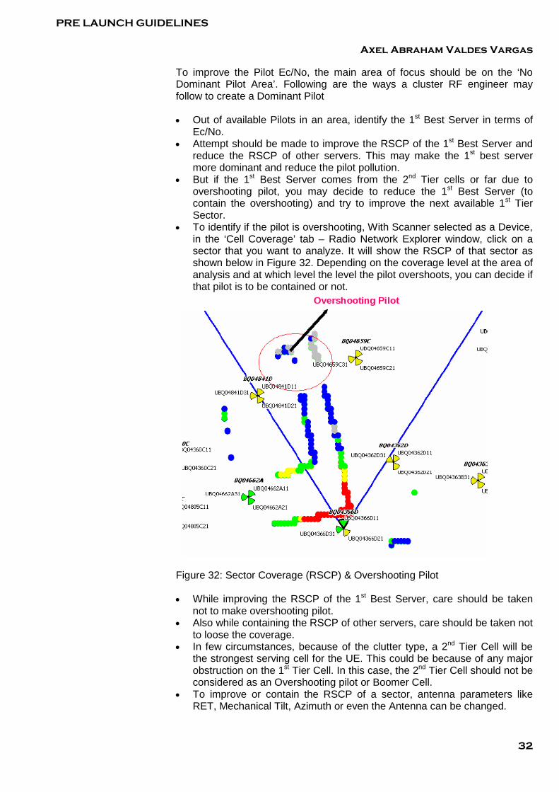
• To identify if the pilot is overshooting, With Scanner selected as a Device, in the ‘Cell Coverage’ tab – Radio Network Explorer window, click on a sector that you want to analyze. It will show the RSCP of that sector as shown below in Figure 32. Depending on the coverage level at the area of analysis and at which level the level the pilot overshoots, you can decide if that pilot is to be contained or not.
Figure 32: Sector Coverage (RSCP) & Overshooting Pilot • While improving the RSCP of the 1st Best Server, care should be taken
not to make overshooting pilot. • Also while containing the RSCP of other servers, care should be taken not
to loose the coverage. • In few circumstances, because of the clutter type, a 2nd Tier Cell will be
the strongest serving cell for the UE. This could be because of any major obstruction on the 1st Tier Cell. In this case, the 2nd Tier Cell should not be considered as an Overshooting pilot or Boomer Cell.
• To improve or contain the RSCP of a sector, antenna parameters like RET, Mechanical Tilt, Azimuth or even the Antenna can be changed.

PRE LAUNCH GUIDELINES
Axel Abraham Valdes Vargas
33
• In few circumstances where if you are not able to contain the overshooting pilot or reduce the pilot pollution, 3G and 2G (if required) Neighbor Lists may not be modified accordingly. This may make sure there is no drop calls in the pilot pollution or overshooting areas.
• Neighbor list need to be corrected incase of any Missing Neighbors. • IRAT Handover boundary may need to be tuned if there is a early or
delayed IRAT HO. ( Not Required During Cluster Tuning) • On a high level, you may decide to tune the Soft Handover Parameters to
reduce the call drops due to handover failures of pilot pollution. But this is not recommended during cluster tuning phase.
4.4.4.3. UE Transmit Power – UL Coverage UE Transmit Power Plot can be taken using the Handset making Long Call (MS3). It is recommended to use the Long Call Handset, for the fact that, the UE transmits the right power when it is on call. During idle mode UE does not transmit continuously. To display the UE TX PWR, in the Summary Dashboard, Select the Long Call Handset (MS3) and then click ‘Radio Network’. In the Radio Network Explorer window, select ‘UE_TxPow’ from the Attributes. This will display the UE Transmit Power in the map window as shown below in Figure 34.
Figure 34: UE Transmit Power Plot - UL Coverage Main objective of checking the UE Transmit Power is to verify the Path Balance. Where ever there is a good RSCP, UE should transmit at a lower power. The UL & DL may not be balanced due to various factors such as like differences in Downlink and Uplink Power Control algorithms, Interference conditions, Traffic conditions, etc. To verify the path balance visually, from the UE TX Power Plot, identify the areas of high UE Transmit Power (Say > 0 dBm) and then look at the RSCP and Ec/No Plots. If you see poor RSCP, it could be a poor coverage area. In this case, an attempt should be made to improve the coverage. If you see a poor Ec/No with a good RSCP, it could be due to interference or high traffic. If it is an interference issue due to pilot pollution or overshooting pilot, an attempt should be made to improve the Pilot Ec/No.

PRE LAUNCH GUIDELINES
Axel Abraham Valdes Vargas
34
In few circumstances, UE Transmit Power could be higher with a good RSCP and Ec/No. This indicates an issue with the Uplink. This may be due to any of the following issues.
• TMA, Cable, Antenna, Node B Hardware issues • Improper Uplink Power Control Parameters • Improper IRAT Trigger • Improper Cell Selection / Reselection parameters • Improper Node B parameters like, ulAttenuation, dlAttenuation, TMA
Insertion Loss, TMA Gain, etc. • External Uplink Interference
If any hardware issues suspected at the site, Alarm history may be verified and if required a Cell technician may be sent to the site to verify the hardware, TMA, Antenna, feeders, etc. You can also verify the level of RWTP reported at Node B. Higher RWTP could be an indication of External Uplink interference, Hardware Issues, etc. 4.4.4.4.Downlink BLER – Quality Quality of Downlink in terms of BLER can be displayed in the Event Explorer Window by choosing the Attribute ‘Uu_TrCh_DownlinkBlerAgg’. As per the U12 Contract Specifications KPI table, DL BLER should be less than or equal to 2% in 95% of the samples. This can be calculated using the BLER Legend displayed on the right side of the Map window. BLER can be displayed and the BLER KPI can be calculated for all the handsets (MS2, MS3 and MS4). For MS4 making PS calls, the KPI for DL BLER is less than or equal to 5% in 95% of drive samples. A sample plot of DL BLER is shown below in Figure 35.
Figure 35: DL BLER Plot In most of the cases the required KPI in terms of DL-BLER will be met. If the KPI is not met, a visual verification over the plot would reveal the areas of poor BLER. Following could be the reasons why the DL BLER can be bad.

PRE LAUNCH GUIDELINES
Axel Abraham Valdes Vargas
35
• Poor Ec/No (due to Pilot pollution, overshooting pilot, Missing Neighbors, etc)
• Poor Coverage (poor RSCP and Ec/No) Improving RSCP and Ec/No would generally bring the DL BLER up to meet the required KPI. 4.4.4.5.Coverage Analysis – Deliverables Following is the list of deliverables at the end of Coverage Analysis for every cluster / market.
• RSCP Coverage Statistics / Distribution. Percentage of drive samples with RSCP > -104 dBm
• Ec/No Statistics / Distribution. Percentage of drive samples with Ec/No > -14 dBm
• UE TX PWR Statistics / Distribution. Percentage of drive samples with UE TX PWR < 18 dBm
• DL BLER Statistics / Distribution. Percentage of drive samples with DL BLER < 2%
• List of Changes in Sites / Parameters to achieve the required coverage KPIs. An example is shown below
4.4.5.Pilot Pollution Analysis Since WCDMA utilizes N=1 frequency reuse, inter-cell interference is an ever present issue. System performance and overall service quality are directly related to the degree to which interference can be controlled. In CDMA systems, interference is mitigated by soft handover. However, increased soft handoff results in increased network resource utilization (e.g. RF power, OVSF codes, channel elements, Iub capacity, and RNC processing load). In addition, HSDPA does not utilize soft handover and is therefore highly susceptible to system interference. The concept of pilot pollution has created a lot of industry buzz; most engineers realize that pollution is “bad”. But it is important to keep in mind the reasons why pollution is bad. Although pollution analysis utilizes the pilot energy as an indication of potential interference, it is not actually the pilot that is the problem. Typically the pilot (CPICH) is less than or equal to ten percent of the total potential power of the cell. Therefore, it is this potential energy from a loaded cell that will cause the interference. That being the case, the objective of pollution analysis is to identify areas where pollution exists, and take actions to improve the coverage in that area to reduce interference. The classical definition of pilot pollution is a situation in which the received power (RSSI) is high, but Ec/No of the best server is low. This definition has evolved over time into a more quantifiable one, namely, a situation in which four or more pilots are received within 5 dB of each other, including the strongest pilot. This definition is implemented in Actix when the advanced option Uu_Scan_TooManyServersThreshold was set to 5 dB. During the analysis process, scanner data will be used to identify areas of high pilot pollution. This analysis should allow the engineer to quickly identify sites that are over/under propagating, and recommend corrective action. 4.4.5.1.Spotlight Cell Pollution Analysis

PRE LAUNCH GUIDELINES
Axel Abraham Valdes Vargas
36
To begin the pilot pollution analysis, click the Radio Network link on the Summary Dashboard screen of the Actix Spotlight project. After the Radio Network screen appears, select the Cell Pilot Pollution tab to move to the pollution analysis screen (see Figure 36). At this point, it may be useful to describe some terms, as well as features available on the Cell Pilot Pollution tab of the Radio Network Explorer. Before beginning the pollution analysis, it is important to select the correct type of analysis. Referring to Figure 36, the Analysis drop down menu allows the user to choose one of two types of pollution analysis (i.e. Pilot Pollution – Scanner, or Too Many Servers – Scanner). The default option is Pilot Pollution – Scanner. This option flags measurement events when four or more pilots are measured less that some pre-defined threshold (default = 15 dB). This analysis is more appropriate for IS-95 or CDMA1x technologies which have fixed thresholds for adding and removing cells to the active set. On the other hand, WCDMA uses reporting ranges that track the strongest pilot in the active set. Therefore, it is more appropriate to use the Too Many Servers – Scanner option. This option flags bins when four or more pilots are measured within 5 dB of the strongest pilot (as configured Threshold Editor).
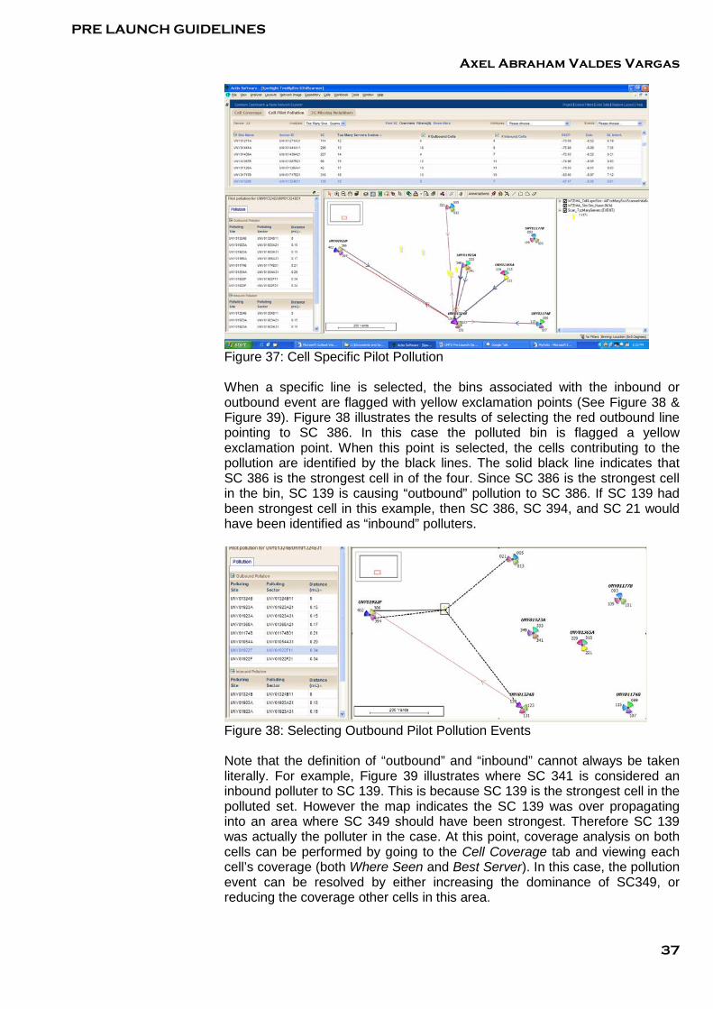
Figure 36: Cell Pilot Pollution Screen Referring to Figure 36, the upper third of the Radio Network Explorer contains statistical data, based on a per cell basis. The data provided includes Too Many Servers Events, # of Outbound Cells, and # of Inbound Cells. When a specific cell is selected, pollution events involving this cell are displayed on the map (see Figure 37). In addition, the other cells involved are listed on the left side of the Network Explorer. In this example, SC 139 is selected, and the Too Many Servers events related to this cell are mapped. The red lines point to cells that are polluted by SC 139. On the other hand, the blue lines originate from cells that are polluting SC 139. These definitions are based on which cell is the strongest cell when a Too Many Servers event occurs. If this event occurs and SC 139 is the strongest, it is considered an inbound event. If this event occurs and SC 139 is not the strongest, then it is considered an outbound event. When a cell is initially selected, the inbound bins associated with the inbound events are flagged with yellow exclamation points (as shown in Figure 37).
PRE LAUNCH GUIDELINES
Axel Abraham Valdes Vargas
37
Figure 37: Cell Specific Pilot Pollution When a specific line is selected, the bins associated with the inbound or outbound event are flagged with yellow exclamation points (See Figure 38 & Figure 39). Figure 38 illustrates the results of selecting the red outbound line pointing to SC 386. In this case the polluted bin is flagged a yellow exclamation point. When this point is selected, the cells contributing to the pollution are identified by the black lines. The solid black line indicates that SC 386 is the strongest cell in of the four. Since SC 386 is the strongest cell in the bin, SC 139 is causing “outbound” pollution to SC 386. If SC 139 had been strongest cell in this example, then SC 386, SC 394, and SC 21 would have been identified as “inbound” polluters.
Figure 38: Selecting Outbound Pilot Pollution Events Note that the definition of “outbound” and “inbound” cannot always be taken literally. For example, Figure 39 illustrates where SC 341 is considered an inbound polluter to SC 139. This is because SC 139 is the strongest cell in the polluted set. However the map indicates the SC 139 was over propagating into an area where SC 349 should have been strongest. Therefore SC 139 was actually the polluter in the case. At this point, coverage analysis on both cells can be performed by going to the Cell Coverage tab and viewing each cell’s coverage (both Where Seen and Best Server). In this case, the pollution event can be resolved by either increasing the dominance of SC349, or reducing the coverage other cells in this area.

PRE LAUNCH GUIDELINES
Axel Abraham Valdes Vargas
38
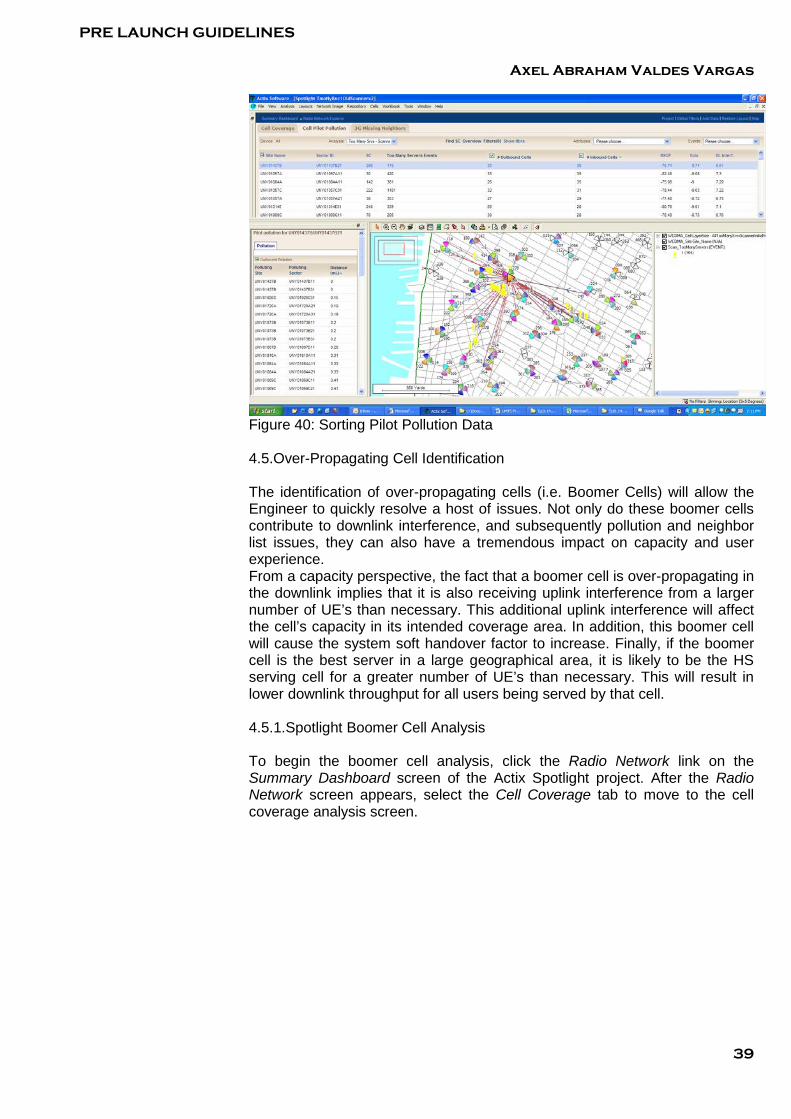
Figure 39: Selecting Inbound Pilot Pollution Events 4.4.5.2.Identifying Polluting Cells Obviously the Engineer can indentify polluting cells by simply clicking on each cell and observing the Too Many Server events. However this can be a time consuming process. The preferred approach would identify the cells that are the highest contributors to pollution. In this manner, corrective action can be taken on these offending cells, thus achieving the greatest amount of improvement with the lowest amount of effort and potential cost. As previously described (see Figure 36), the upper third of the Radio Network Explorer contains statistical data, based on a per cell basis. The data provided includes Too Many Servers Events, # of Outbound Cells, and # of Inbound Cells. By clicking the column headings for this data, the results can be sorted in descending or ascending order. For example, in Figure 39, the data for the # of Inbound Cells was sorted in descending order. By sorting on these columns, cells that are involved with a high frequency of pollution events can be identified. It should be noted that the Too Many Servers Events provides contradicting information and should be used with caution. It does not indicate the number of polluted bins containing a selected SC (although this would be quite useful). Nor does is provide the sum of inbound and outbound events. It is likely to be based on un-binned measurements which can result in unpredictable results (e.g. zero velocity scanner data collected while test vehicle was stopped).
PRE LAUNCH GUIDELINES
Axel Abraham Valdes Vargas
39
Figure 40: Sorting Pilot Pollution Data 4.5.Over-Propagating Cell Identification The identification of over-propagating cells (i.e. Boomer Cells) will allow the Engineer to quickly resolve a host of issues. Not only do these boomer cells contribute to downlink interference, and subsequently pollution and neighbor list issues, they can also have a tremendous impact on capacity and user experience. From a capacity perspective, the fact that a boomer cell is over-propagating in the downlink implies that it is also receiving uplink interference from a larger number of UE’s than necessary. This additional uplink interference will affect the cell’s capacity in its intended coverage area. In addition, this boomer cell will cause the system soft handover factor to increase. Finally, if the boomer cell is the best server in a large geographical area, it is likely to be the HS serving cell for a greater number of UE’s than necessary. This will result in lower downlink throughput for all users being served by that cell. 4.5.1.Spotlight Boomer Cell Analysis To begin the boomer cell analysis, click the Radio Network link on the Summary Dashboard screen of the Actix Spotlight project. After the Radio Network screen appears, select the Cell Coverage tab to move to the cell coverage analysis screen.
PRE LAUNCH GUIDELINES
Axel Abraham Valdes Vargas
40
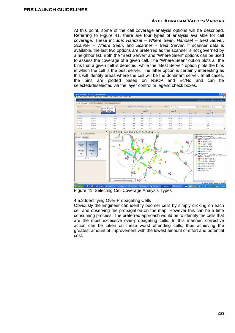
At this point, some of the cell coverage analysis options will be described. Referring to Figure 41, there are four types of analysis available for cell coverage. These include: Handset – Where Seen, Handset – Best Server, Scanner – Where Seen, and Scanner – Best Server. If scanner data is available, the last two options are preferred as the scanner is not governed by a neighbor list. Both the “Best Server” and “Where Seen” options can be used to assess the coverage of a given cell. The “Where Seen” option plots all the bins that a given cell is detected, while the “Best Server” option plots the bins in which the cell is the best server. The latter option is certainly interesting as this will identify areas where the cell will be the dominant server. In all cases, the bins are plotted based on RSCP and Ec/No and can be selected/deselected via the layer control or legend check boxes.
Figure 41: Selecting Cell Coverage Analysis Types 4.5.2.Identifying Over-Propagating Cells Obviously the Engineer can identify boomer cells by simply clicking on each cell and observing the propagation on the map. However this can be a time consuming process. The preferred approach would be to identify the cells that are the most excessive over-propagating cells. In this manner, corrective action can be taken on these worst offending cells, thus achieving the greatest amount of improvement with the lowest amount of effort and potential cost.

PRE LAUNCH GUIDELINES
Axel Abraham Valdes Vargas
41
One method of achieving this with Actix Spotlight is to use statistic data based on thresholds for cell radius. This method counts the number of times a cell’s pilot is detected outside its defined cell radius. By sorting on this data, the cells with the highest amount of overspill can be identified. This is achieved by clicking the >Dist header in the upper third of the Radio Network Explorer (see Figure 41). This threshold is illustrated the map by the red circle encompassing the selected cell. It should be noted that this data is not based on binned data, and therefore the sorted results may be affected by drive routes and test conditions (e.g. zero velocity measurements will not filtered out). In addition, scrambling code aliasing is a potential risk with any analysis of this type. Because scrambling codes are reused, the tool ties SC measurements to cells based on distance. This assumption is not always correct. In this example (Figure 41), cell NJU70187, SC 130 was detected 13,855 times beyond its cell radius. The plot clearly shows that this is a boomer site. In fact, SC 130 is the best server in measurements taken 12 km from the site. The value of this cell radius is configured by one of two means. The Threshold Editor can be used to define the SL_Overspill_Dist_Threshold (see Figure 42). This is a global setting and should be adjusted based on the morphology and site density of the area to be analyzed. Alternatively, cell specific radiuses can be defined by the MaxServerDist parameter in the cellref file. If this is defined, its value will supersede the global parameter SL_Overspill_Dist_Threshold.
Figure 42: Cell Radius Global Setting In addition to using the cell radius method to identify boomer cells, pollution and neighbor list analysis will typically identify over-propagating cells as well. In addition, some OSS tools may identify boomer cells once there is sufficient traffic. For example, the Ericsson WNCS missing neighbor tool provided distance information for both defined and missing neighbors, which can be used to identify boomers. Once a boomer cell is identified, it is obvious that corrective action should be taken (e.g. tilts, ACL, etc.). However, if the over-propagating coverage can not be corrected, the boomer cell must be added to the affected cells neighbor list (and vice-versa). 4.6.UMTS Neighbor List Analysis
PRE LAUNCH GUIDELINES
Axel Abraham Valdes Vargas
42
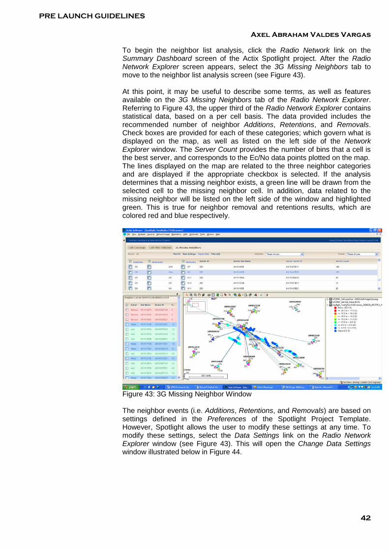
To begin the neighbor list analysis, click the Radio Network link on the Summary Dashboard screen of the Actix Spotlight project. After the Radio Network Explorer screen appears, select the 3G Missing Neighbors tab to move to the neighbor list analysis screen (see Figure 43). At this point, it may be useful to describe some terms, as well as features available on the 3G Missing Neighbors tab of the Radio Network Explorer. Referring to Figure 43, the upper third of the Radio Network Explorer contains statistical data, based on a per cell basis. The data provided includes the recommended number of neighbor Additions, Retentions, and Removals. Check boxes are provided for each of these categories; which govern what is displayed on the map, as well as listed on the left side of the Network Explorer window. The Server Count provides the number of bins that a cell is the best server, and corresponds to the Ec/No data points plotted on the map. The lines displayed on the map are related to the three neighbor categories and are displayed if the appropriate checkbox is selected. If the analysis determines that a missing neighbor exists, a green line will be drawn from the selected cell to the missing neighbor cell. In addition, data related to the missing neighbor will be listed on the left side of the window and highlighted green. This is true for neighbor removal and retentions results, which are colored red and blue respectively.
Figure 43: 3G Missing Neighbor Window The neighbor events (i.e. Additions, Retentions, and Removals) are based on settings defined in the Preferences of the Spotlight Project Template. However, Spotlight allows the user to modify these settings at any time. To modify these settings, select the Data Settings link on the Radio Network Explorer window (see Figure 43). This will open the Change Data Settings window illustrated below in Figure 44.
PRE LAUNCH GUIDELINES
Axel Abraham Valdes Vargas
43
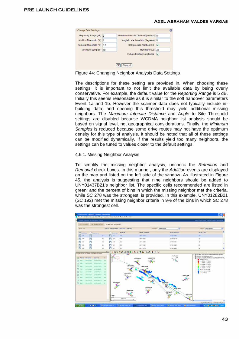
Figure 44: Changing Neighbor Analysis Data Settings The descriptions for these setting are provided in. When choosing these settings, it is important to not limit the available data by being overly conservative. For example, the default value for the Reporting Range is 5 dB. Initially this seems reasonable as it is similar to the soft handover parameters Event 1a and 1b. However the scanner data does not typically include in-building data; and opening this threshold may yield additional missing neighbors. The Maximum Intersite Distance and Angle to Site Threshold settings are disabled because WCDMA neighbor list analysis should be based on signal level, not geographical considerations. Finally, the Minimum Samples is reduced because some drive routes may not have the optimum density for this type of analysis. It should be noted that all of these settings can be modified dynamically. If the results yield too many neighbors, the settings can be tuned to values closer to the default settings. 4.6.1. Missing Neighbor Analysis To simplify the missing neighbor analysis, uncheck the Retention and Removal check boxes. In this manner, only the Addition events are displayed on the map and listed on the left side of the window. As illustrated in Figure 45, the analysis is suggesting that nine neighbors should be added to UNY01437B21’s neighbor list. The specific cells recommended are listed in green; and the percent of bins in which the missing neighbor met the criteria, while SC 278 was the strongest, is provided. In this example, UNY01282B21 (SC 192) met the missing neighbor criteria in 9% of the bins in which SC 278 was the strongest cell.

PRE LAUNCH GUIDELINES
Axel Abraham Valdes Vargas
44
Figure 45: Viewing Missing Neighbor Events To focus on this specific missing neighbor, either select the green line between SC 286 and SC 192, or select cell UNY01282B21 from the list of additions on the left side of the Radio Network Explorer window. This will display the bins that triggered the missing neighbor event for these SC pair (see Figure 46). In this case, it appears that the over propagation of SC 286, and the unexpected propagation of SC 192, resulted in the missing neighbor event occurring. These results can be corroborated by going the Cell Coverage tab and view each cells coverage (both Where Seen and Best Server). In this example, additional coverage analysis should be initiated to attempt to correct the coverage issue of both cells. However, if the coverage issues cannot be corrected, these two cells should be added to each other’s neighbor list. This procedure should be repeated for each missing neighbor event.
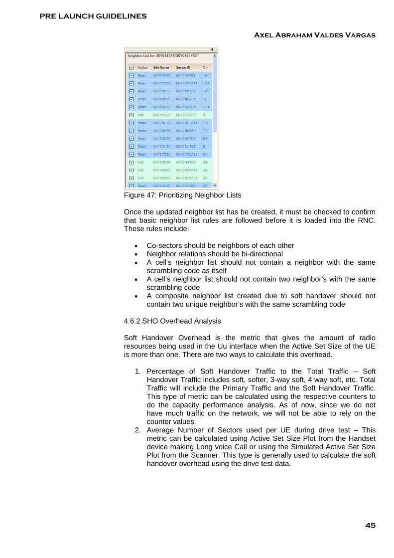
Figure 46: Focusing on Specific Missing Neighbors In addition to performing missing neighbor analysis, the validity of existing neighbors can be confirmed. This is accomplished by using the Retention and Removal features of the 3G Neighbor Analysis. An existing neighbor will be flagged for Removal if it does not have a sufficient percentage of bins that meet the Reporting Range (as defined by the Removal Threshold). On the other hand, if an existing neighbor meets this criterion, it will be flagged for Retention. In both cases, the analysis can be corroborated by using the Cell Coverage tab and viewing coverage of the two neighbor cells. Caution should be used when removing neighbors from a cell’s neighbor list. Because this analysis is based on drive testing, certain areas within a cell’s coverage (including in-building) will be excluded from the analysis. A preferred method for removing neighbors from a cell’s neighbor list is to utilized UTRAN counters or OSS tools (e.g. Ericsson’s WNCS report). Once Additions, Removals, and Retentions have been confirmed, they can be sorted in descending order to determine priority within the cell’s neighbor list. This is accomplished by clicking the “%” button indicated in Figure 47. At this point the list can be exported by clicking the Export Data link on the Radio Network Explorer window. Only the cells with their checkbox checked will be exported.
PRE LAUNCH GUIDELINES
Axel Abraham Valdes Vargas
45
Figure 47: Prioritizing Neighbor Lists Once the updated neighbor list has be created, it must be checked to confirm that basic neighbor list rules are followed before it is loaded into the RNC. These rules include:
• Co-sectors should be neighbors of each other • Neighbor relations should be bi-directional • A cell’s neighbor list should not contain a neighbor with the same
scrambling code as itself • A cell’s neighbor list should not contain two neighbor’s with the same
scrambling code • A composite neighbor list created due to soft handover should not
contain two unique neighbor’s with the same scrambling code 4.6.2.SHO Overhead Analysis Soft Handover Overhead is the metric that gives the amount of radio resources being used in the Uu interface when the Active Set Size of the UE is more than one. There are two ways to calculate this overhead.
1. Percentage of Soft Handover Traffic to the Total Traffic – Soft Handover Traffic includes soft, softer, 3-way soft, 4 way soft, etc. Total Traffic will include the Primary Traffic and the Soft Handover Traffic. This type of metric can be calculated using the respective counters to do the capacity performance analysis. As of now, since we do not have much traffic on the network, we will not be able to rely on the counter values.
2. Average Number of Sectors used per UE during drive test – This metric can be calculated using Active Set Size Plot from the Handset device making Long voice Call or using the Simulated Active Set Size Plot from the Scanner. This type is generally used to calculate the soft handover overhead using the drive test data.
PRE LAUNCH GUIDELINES
Axel Abraham Valdes Vargas
46
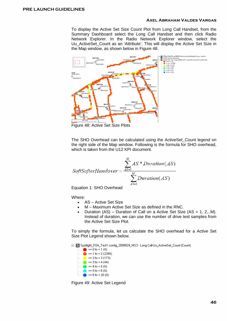
To display the Active Set Size Count Plot from Long Call Handset, from the Summary Dashboard select the Long Call Handset and then click Radio Network Explorer. In the Radio Network Explorer window, select the Uu_ActiveSet_Count as an ‘Attribute’. This will display the Active Set Size in the Map window, as shown below in Figure 48.
Figure 48: Active Set Size Plots The SHO Overhead can be calculated using the ActiveSet_Count legend on the right side of the Map window. Following is the formula for SHO overhead, which is taken from the U12 KPI document.
Equation 1: SHO Overhead Where:
• AS – Active Set Size • M – Maximum Active Set Size as defined in the RNC. • Duration (AS) – Duration of Call on a Active Set Size (AS = 1, 2,..M).
Instead of duration, we can use the number of drive test samples from the Active Set Size Plot.
To simply the formula, let us calculate the SHO overhead for a Active Set Size Plot Legend shown below.
Figure 49: Active Set Legend
PRE LAUNCH GUIDELINES
Axel Abraham Valdes Vargas
47
SHO Overhead = (1*2295 + 2*173 + 3*44) / (2295+173+44) = 1.103 This is amazingly a very good value for the SHO overhead. This is because the UE is with only one SC in Active Set for most of the time as we see in the Active Set Size Plot above. This indicates the network has got very less internal interference and enhanced capacity. As per the U12 KPI document, the threshold for SHO overhead is 1.6. Similar calculation for SHO Overhead can be done using the Simulative Active Set Size Plot using the Scanner Device as well. If the KPI for SHO Overhead is not met the following steps may be taken by the Cluster RF engineer.
• Identify the areas with higher Active Set Size Plot • Verify the Pilot Pollution Plot in that area. If there is a Pilot Pollution,
steps should be taken to reduce it. • Also verify the ‘Too Many Server Plot’. This is a good indication of
Active Set Size. Coverage in terms of Ec/No and RSCP may be good. But, ‘Too Many Servers’ increases the SHO overhead and reduces the overall System Capacity.
• If there are any ‘Too Many Server’ noticed, steps should be taken to reduce coverage from 2nd, 3rd or 4th, etc., best servers while retaining or improving the coverage from 1st Best Server.
• Coverage reduction or improvement can be done by changing RET, Mechanical Tilt, Azimuth or Antenna, if required.
• While doing this, care should be taken not to lose the coverage of 2nd, 3rd or 4th, etc., best servers and increase the overshooting pilot from 1st Best Server.
• Incase if there is any irresolvable Pilot Pollution or Too Many Server issues, optimizing the Soft Handover Parameters will help reducing the SHO overhead. But this should be done as the last measure, because any change in SHO parameters may impact the entire RNC.
4.7.Access Failure Analysis The following section provides a summary of the Call Setup procedure. The fundamental steps required in accessing a UMTS network is similar for both CS and PS services. In both cases the UE utilizes the same random access procedure to request establishment of a RRC Connection with the RNC. If dedicated resources are available to setup this radio link, an RRC Connection will be established with the RNC. Once an RRC Connection is established with the RNC, the Core Network (CN) is signaled to establish an Iu connection between the CN and RNC. At this time the core network initiates security procedures such as Authentication and Ciphering. After the security procedures are completed, the UE requests services from the Core Network. The CN then requests the establishment of a Radio Access Bearer (RAB) with the RNC to support the requested services. If this RAB is established, the RNC will acknowledge the CN request and a successful access will have occurred. Alternatively, if any of these steps fail, an access failure will occur. Therefore, there are essentially 3 procedures that need to be completed before call setup is deemed to be successful.

PRE LAUNCH GUIDELINES
Axel Abraham Valdes Vargas
48
• RACH Access Procedure – Used to access the network to initiate various procedures including network updates, voice & data call setup, paging responses
• RRC Connection Setup Procedure – Used to establish signaling radio bearers and provide an interface to the NAS layer
• Pre-RAB & RAB Setup Procedure – Used to establish end to end connection and complete authentication & security procedures whilst establishing DCH for a specific service type
It is recommended that users familiarize themselves with content from this document to understand the Access Setup procedures in greater detail. The Access failure is the product of the RRC Connection Failure, NAS Setup Failure and the RAB Establishment Failure. RRC Connection Success shall be counted when the RNC receives a RRC Setup Complete from the UE. NAS Setup shall be considered successful when the signaling messages in the call flow during call setup flow is successfully completed by relevant Network Elements. A RAB is considered successfully established when the RAB Assignment Response is sent by RNC to the CN. An AMR call flow is shown below to illustrate this:
Figure 50: AMR Call Flow The current definitions for Access Failures as per the contract are:
Equation 2: CSV Access Failure Definition
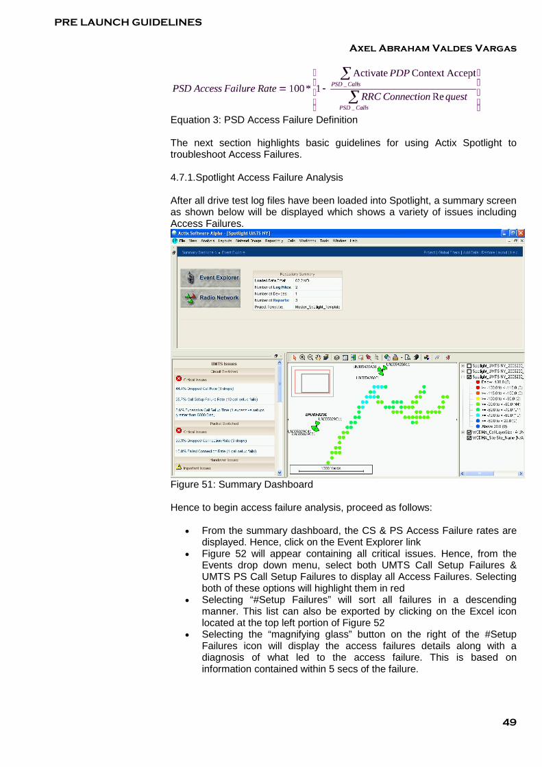
PRE LAUNCH GUIDELINES
Axel Abraham Valdes Vargas
49
Equation 3: PSD Access Failure Definition The next section highlights basic guidelines for using Actix Spotlight to troubleshoot Access Failures. 4.7.1.Spotlight Access Failure Analysis After all drive test log files have been loaded into Spotlight, a summary screen as shown below will be displayed which shows a variety of issues including Access Failures.
Figure 51: Summary Dashboard Hence to begin access failure analysis, proceed as follows:
• From the summary dashboard, the CS & PS Access Failure rates are displayed. Hence, click on the Event Explorer link
• Figure 52 will appear containing all critical issues. Hence, from the Events drop down menu, select both UMTS Call Setup Failures & UMTS PS Call Setup Failures to display all Access Failures. Selecting both of these options will highlight them in red
• Selecting “#Setup Failures” will sort all failures in a descending manner. This list can also be exported by clicking on the Excel icon located at the top left portion of Figure 52
• Selecting the “magnifying glass” button on the right of the #Setup Failures icon will display the access failures details along with a diagnosis of what led to the access failure. This is based on information contained within 5 secs of the failure.
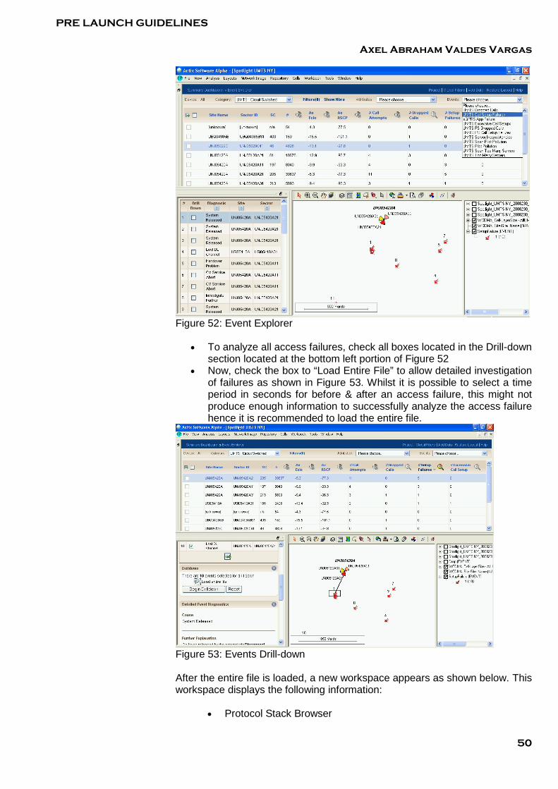
PRE LAUNCH GUIDELINES
Axel Abraham Valdes Vargas
50
Figure 52: Event Explorer
• To analyze all access failures, check all boxes located in the Drill-down section located at the bottom left portion of Figure 52
• Now, check the box to “Load Entire File” to allow detailed investigation of failures as shown in Figure 53. Whilst it is possible to select a time period in seconds for before & after an access failure, this might not produce enough information to successfully analyze the access failure hence it is recommended to load the entire file.
Figure 53: Events Drill-down After the entire file is loaded, a new workspace appears as shown below. This workspace displays the following information:
• Protocol Stack Browser
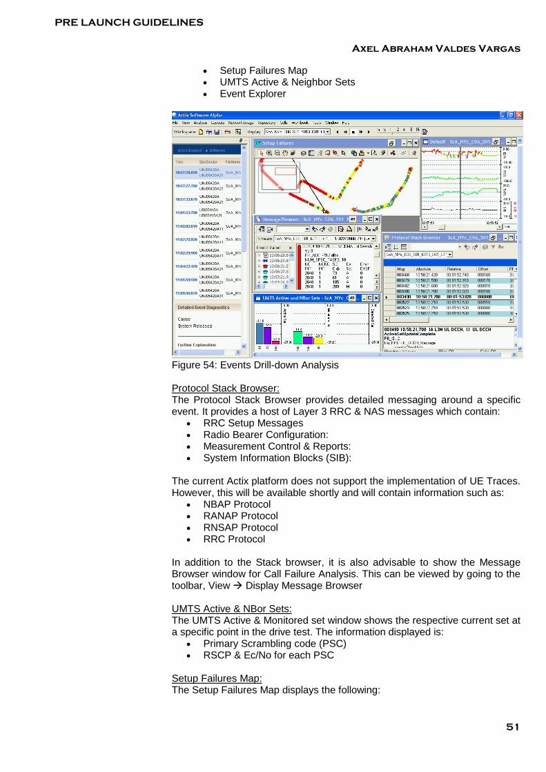
PRE LAUNCH GUIDELINES
Axel Abraham Valdes Vargas
51
• Setup Failures Map • UMTS Active & Neighbor Sets • Event Explorer
Figure 54: Events Drill-down Analysis Protocol Stack Browser: The Protocol Stack Browser provides detailed messaging around a specific event. It provides a host of Layer 3 RRC & NAS messages which contain:
• RRC Setup Messages • Radio Bearer Configuration: • Measurement Control & Reports: • System Information Blocks (SIB):
The current Actix platform does not support the implementation of UE Traces. However, this will be available shortly and will contain information such as:
• NBAP Protocol • RANAP Protocol • RNSAP Protocol • RRC Protocol
In addition to the Stack browser, it is also advisable to show the Message Browser window for Call Failure Analysis. This can be viewed by going to the toolbar, View Display Message Browser UMTS Active & NBor Sets: The UMTS Active & Monitored set window shows the respective current set at a specific point in the drive test. The information displayed is:
• Primary Scrambling code (PSC) • RSCP & Ec/No for each PSC
Setup Failures Map: The Setup Failures Map displays the following:
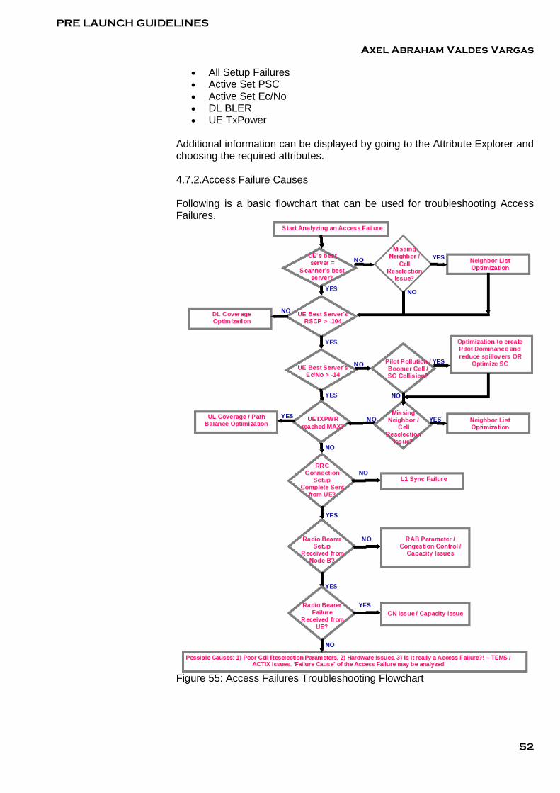
PRE LAUNCH GUIDELINES
Axel Abraham Valdes Vargas
52
• All Setup Failures • Active Set PSC • Active Set Ec/No • DL BLER • UE TxPower
Additional information can be displayed by going to the Attribute Explorer and choosing the required attributes. 4.7.2.Access Failure Causes Following is a basic flowchart that can be used for troubleshooting Access Failures.
Figure 55: Access Failures Troubleshooting Flowchart
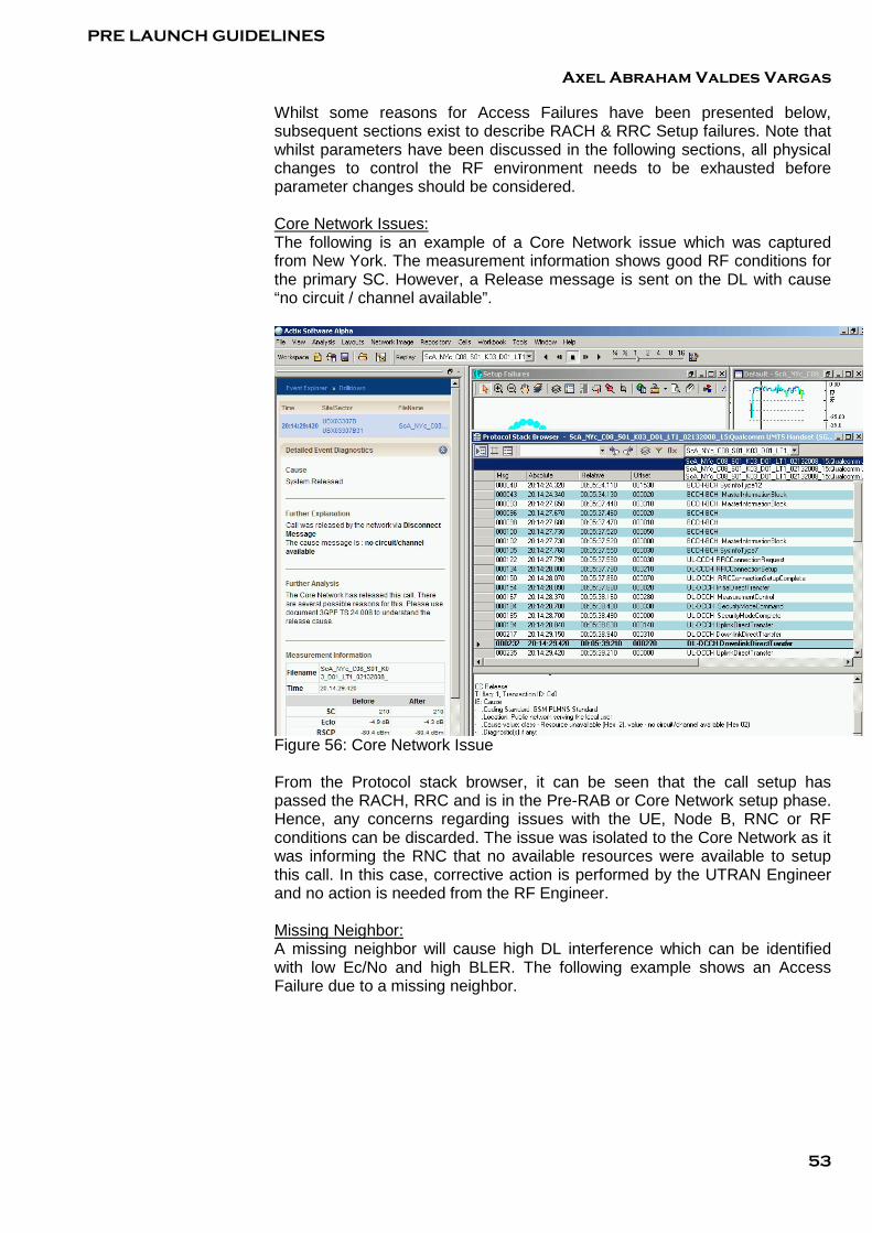
PRE LAUNCH GUIDELINES
Axel Abraham Valdes Vargas
53
Whilst some reasons for Access Failures have been presented below, subsequent sections exist to describe RACH & RRC Setup failures. Note that whilst parameters have been discussed in the following sections, all physical changes to control the RF environment needs to be exhausted before parameter changes should be considered. Core Network Issues: The following is an example of a Core Network issue which was captured from New York. The measurement information shows good RF conditions for the primary SC. However, a Release message is sent on the DL with cause “no circuit / channel available”.
Figure 56: Core Network Issue From the Protocol stack browser, it can be seen that the call setup has passed the RACH, RRC and is in the Pre-RAB or Core Network setup phase. Hence, any concerns regarding issues with the UE, Node B, RNC or RF conditions can be discarded. The issue was isolated to the Core Network as it was informing the RNC that no available resources were available to setup this call. In this case, corrective action is performed by the UTRAN Engineer and no action is needed from the RF Engineer. Missing Neighbor: A missing neighbor will cause high DL interference which can be identified with low Ec/No and high BLER. The following example shows an Access Failure due to a missing neighbor.
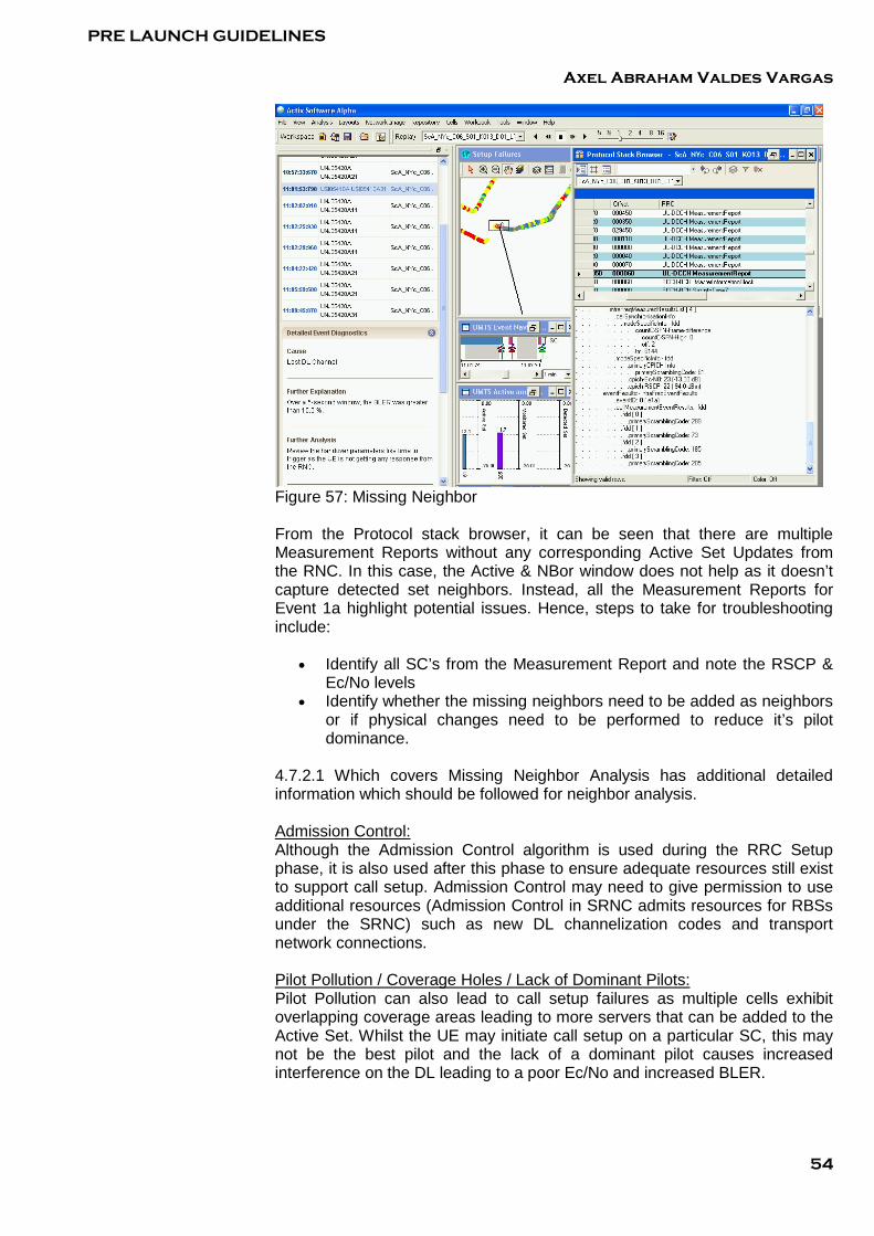
PRE LAUNCH GUIDELINES
Axel Abraham Valdes Vargas
54
Figure 57: Missing Neighbor From the Protocol stack browser, it can be seen that there are multiple Measurement Reports without any corresponding Active Set Updates from the RNC. In this case, the Active & NBor window does not help as it doesn’t capture detected set neighbors. Instead, all the Measurement Reports for Event 1a highlight potential issues. Hence, steps to take for troubleshooting include:
• Identify all SC’s from the Measurement Report and note the RSCP & Ec/No levels
• Identify whether the missing neighbors need to be added as neighbors or if physical changes need to be performed to reduce it’s pilot dominance.
4.7.2.1 Which covers Missing Neighbor Analysis has additional detailed information which should be followed for neighbor analysis. Admission Control: Although the Admission Control algorithm is used during the RRC Setup phase, it is also used after this phase to ensure adequate resources still exist to support call setup. Admission Control may need to give permission to use additional resources (Admission Control in SRNC admits resources for RBSs under the SRNC) such as new DL channelization codes and transport network connections. Pilot Pollution / Coverage Holes / Lack of Dominant Pilots: Pilot Pollution can also lead to call setup failures as multiple cells exhibit overlapping coverage areas leading to more servers that can be added to the Active Set. Whilst the UE may initiate call setup on a particular SC, this may not be the best pilot and the lack of a dominant pilot causes increased interference on the DL leading to a poor Ec/No and increased BLER.

PRE LAUNCH GUIDELINES
Axel Abraham Valdes Vargas
55
A UE may initiate a call but due to the RF environment enter a coverage hole which leads to an access failure. The network has been designed in loaded conditions for service areas that meet CPICH RSCP (Outdoor) at -104dBm & Ec/No at -12dB. This service area varies depending on the type of service such as CSD, PS 64, PS 128 & PS 384 kbps. Hence, coverage holes will likely exist in the network in areas failing to meet these internal targets. By looking at the Best Server RSCP, Ec/No & UE TxPower in an area, it can be seen whether a hole indeed exists. To resolve these RF issues, please refer to 4.4 & Section 4.5. Hardware Issues: Hardware issues occurring in the Node B, RNC, Transmission system, antenna system etc; can lead to access failures. If equipment is suspected to be faulty, PM counters can be used to verify if an abnormally high amount of issues such as Access Failures, Drop Calls, Failed SHOs, Low Traffic, Low RRC / RAB Attempts etc; exist. In addition, it is advisable to look at T1 statistics such as Errored & Severely Errored seconds to verify transmission issues. The OSS can also be used to verify if any minor / major / critical alarms exist on specific sites. There will usually be unexplained failures which occurred in good RF conditions that give a clue to hardware issues. However, TEMS & UETR logs if available need to be examined together to rule out RF causes. UE issues could also be causing these failures and testing with different UEs will quickly rule out this issue. 4.7.2.2.RACH Access Troubleshooting The following flowchart expands on the troubleshooting flowchart found in Figure 55. The KPI definitions state that an attempt is made beginning from the RRC Connection Setup phase. However, getting to this phase involves successful acknowledgement of the RACH preambles by the NodeB.

PRE LAUNCH GUIDELINES
Axel Abraham Valdes Vargas
56
Figure 58: RACH Troubleshooting Areas of RACH Analysis are described below: If a NACK is receive by the UE, then examine
• Random Back Off Parameters such as o NB01 (min & max) : Transmitted in SIB 5
If no ACK is received, then examine:
• Parameter Translations such as : o Initial Transmit Power calculation which involves: CPICH RSCP,
CPICH Power (SIB 5), RTWP (SIB 7), ConstantValueCprach (SIB 5)
o MaxTxPowerUL: Needs to be set as per the UE class level assumed in the RF design
o PowerOffsetPO, preambleRetransMax, maxPreambleCycle: Need to ensure that the power increase between subsequent preambles, the number of preamble ramping cycles & maximum number of preamble transmissions in one cycle do not restrict the UE transmit power to be less than the maximum allowed on RACH
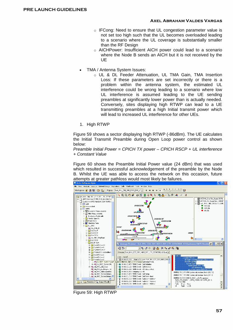
PRE LAUNCH GUIDELINES
Axel Abraham Valdes Vargas
57
o IFCong: Need to ensure that UL congestion parameter value is not set too high such that the UL becomes overloaded leading to a scenario where the UL coverage is substantially smaller than the RF Design
o AICHPower: Insufficient AICH power could lead to a scenario where the Node B sends an AICH but it is not received by the UE
• TMA / Antenna System Issues:
o UL & DL Feeder Attenuation, UL TMA Gain, TMA Insertion Loss: If these parameters are set incorrectly or there is a problem within the antenna system, the estimated UL interference could be wrong leading to a scenario where low UL interference is assumed leading to the UE sending preambles at significantly lower power than is actually needed. Conversely, sites displaying high RTWP can lead to a UE transmitting preambles at a high Initial transmit power which will lead to increased UL interference for other UEs.
1. High RTWP
Figure 59 shows a sector displaying high RTWP (-86dBm). The UE calculates the Initial Transmit Preamble during Open Loop power control as shown below: Preamble Initial Power = CPICH TX power – CPICH RSCP + UL interference + Constant Value Figure 60 shows the Preamble Initial Power value (24 dBm) that was used which resulted in successful acknowledgement of the preamble by the Node B. Whilst the UE was able to access the network on this occasion, future attempts at greater pathloss would most likely be failures.
Figure 59: High RTWP

PRE LAUNCH GUIDELINES
Axel Abraham Valdes Vargas
58
Figure 60: High Initial Tx Power UL Interference can be analyzed by viewing SIB 7 messages. Whilst this is not processed automatically through Spotlight reports, it can be viewed through Attribute explorer. Hence, it is advisable to plot the UL Interference attribute initially before detailed troubleshooting analysis occurs. This can be easily plotted via Attribute Explorer by clicking on 3G UMTS Uu-RRC BCCH-BCH SysInfoType7 Uu_RRC_SysInfoType7_UL_Interference. Each sector can then be cross-referenced against PM Counters to verify the authenticity of measurements. Sector’ such as the above displaying elevated RTWP levels need to be actioned by viewing the site and checking the complete Antenna / TMA system to verify issues. In addition, spectrum verification activities can also be conducted to rule out external interferers. 4.7.2.3. RRC Setup Troubleshooting The following flowchart expands on the troubleshooting flowchart found in Figure 55.
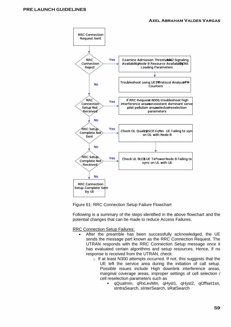
PRE LAUNCH GUIDELINES
Axel Abraham Valdes Vargas
59
Figure 61: RRC Connection Setup Failure Flowchart Following is a summary of the steps identified in the above flowchart and the potential changes that can be made to reduce Access Failures. RRC Connection Setup Failures:
• After the preamble has been successfully acknowledged, the UE sends the message part known as the RRC Connection Request. The UTRAN responds with the RRC Connection Setup message once it has evaluated certain algorithms and setup resources. Hence, if no response is received from the UTRAN, check:
o If at least N300 attempts occurred. If not, this suggests that the UE left the service area during the initiation of call setup. Possible issues include High downlink interference areas, marginal coverage areas, improper settings of cell selection / cell reselection parameters such as
qQualmin, qRxLevMin, qHyst1, qHyst2, qOffset1sn, sIntraSearch, sInterSearch, sRatSearch
PRE LAUNCH GUIDELINES
Axel Abraham Valdes Vargas
60
Marginal Coverage & High Interference areas can be checked by looking at CPICH RSCP, Ec/No plots initially, evaluating the best server and then attempting physical antenna changes or parameter modifications to bring dominant servers if possible
FACH power could be too low. The maxFach1Power & maxFach2Power settings need to be able to cover the entire cell based on an assumed load. Hence, incorrect settings could lead to a situation where the FACH does not cover the entire cell area
o If the UE does receive the RRC Connection Setup message but
fails to send the RRC Connection Setup Complete message, this could be due to L1 synchronization issues between the UE & UTRAN
L1 synchronization needs to occur before the UE can start transmitting on DCH. The UE may not send the complete message unless DL synchronization has occurred. Failure to achieve this could be due to:
Significant differences between the CPICH & DL DPCH coverage areas. Whilst this relationship varies by service type, it is important that the DL power allocated for a UE can at least reach the coverage area dictated by the CPICH parameter setting. The DL DPCH setting can be verified by the Initial, Min & Max Power settings allocated during the Radio Link Setup procedure
o If the UE does send the RRC Connection Setup Complete message but the Node B fails to receive it, this could be due to L1 synchronization issues between the UE & UTRAN.
L1 synchronization needs to occur on both the UL & DL. Whilst the UE may achieve synchronization on the DL which allows it to send UL messages, the Node B still needs to achieve UL synchronization with the UE. Failure to do this could be due to:
UL & DL coverage area imbalances. If the UE is transmitting at or close to maximum power but the Node B is not receiving the messages, the CPICH parameter settings governing the coverage area could be too large
High UL RTWP. Any internal / external sources of continuous / intermittent interference could lead to spikes of high RTWP / BLER which could be causing UL synchronization difficulties. This can be verified with UETR / Agilent / K18 logs as well as SIB 7 messages from the RRC layer of drive test logs
RRC Connection Reject (Congestion / Unspecified):
• During RRC Establishment, the SRNC will check using the Admission Control algorithm if a new Radio Link can be allowed in the cell. It will also check for Node B resource availability and setup AAL2 connections. Hence if a RRC Connection Reject is received with cause “Congestion” or “Unspecified”, check:
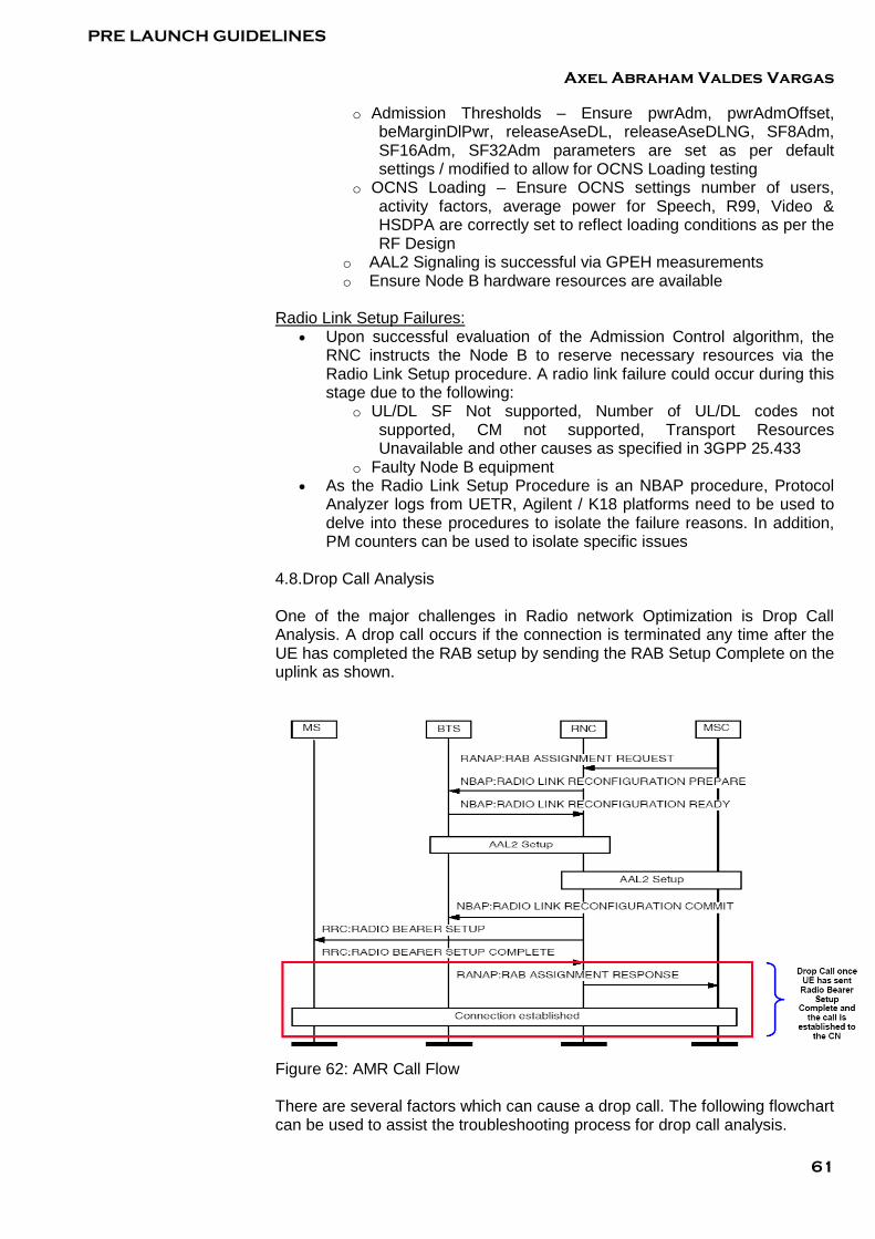
PRE LAUNCH GUIDELINES
Axel Abraham Valdes Vargas
61
o Admission Thresholds – Ensure pwrAdm, pwrAdmOffset, beMarginDlPwr, releaseAseDL, releaseAseDLNG, SF8Adm, SF16Adm, SF32Adm parameters are set as per default settings / modified to allow for OCNS Loading testing
o OCNS Loading – Ensure OCNS settings number of users, activity factors, average power for Speech, R99, Video & HSDPA are correctly set to reflect loading conditions as per the RF Design
o AAL2 Signaling is successful via GPEH measurements o Ensure Node B hardware resources are available
Radio Link Setup Failures:
• Upon successful evaluation of the Admission Control algorithm, the RNC instructs the Node B to reserve necessary resources via the Radio Link Setup procedure. A radio link failure could occur during this stage due to the following:
o UL/DL SF Not supported, Number of UL/DL codes not supported, CM not supported, Transport Resources Unavailable and other causes as specified in 3GPP 25.433
o Faulty Node B equipment • As the Radio Link Setup Procedure is an NBAP procedure, Protocol
Analyzer logs from UETR, Agilent / K18 platforms need to be used to delve into these procedures to isolate the failure reasons. In addition, PM counters can be used to isolate specific issues
4.8.Drop Call Analysis One of the major challenges in Radio network Optimization is Drop Call Analysis. A drop call occurs if the connection is terminated any time after the UE has completed the RAB setup by sending the RAB Setup Complete on the uplink as shown.
Figure 62: AMR Call Flow There are several factors which can cause a drop call. The following flowchart can be used to assist the troubleshooting process for drop call analysis.
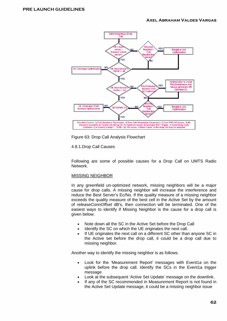
PRE LAUNCH GUIDELINES
Axel Abraham Valdes Vargas
62
Figure 63: Drop Call Analysis Flowchart 4.8.1.Drop Call Causes Following are some of possible causes for a Drop Call on UMTS Radio Network. MISSING NEIGHBOR In any greenfield un-optimized network, missing neighbors will be a major cause for drop calls. A missing neighbor will increase the interference and reduce the Best Server’s Ec/No. If the quality measure of a missing neighbor exceeds the quality measure of the best cell in the Active Set by the amount of releaseConnOffset dB's, then connection will be terminated. One of the easiest ways to identify if Missing Neighbor is the cause for a drop call is given below.
• Note down all the SC in the Active Set before the Drop Call • Identify the SC on which the UE originates the next call. • If UE originates the next call on a different SC other than anyone SC in
the Active set before the drop call, it could be a drop call due to missing neighbor.
Another way to identify the missing neighbor is as follows.
• Look for the ‘Measurement Report’ messages with Event1a on the uplink before the drop call. Identify the SCs in the Event1a trigger message
• Look at the subsequent ‘Active Set Update’ message on the downlink. • If any of the SC recommended in Measurement Report is not found in
the Active Set Update message, it could be a missing neighbor issue

PRE LAUNCH GUIDELINES
Axel Abraham Valdes Vargas
63
• This can also be identified by looking at the Detected Set of the UE. A Scrambling Code which is in the reporting range for ‘event1a’ may be sitting in the Detected Set for a long time without being added into Active Set.
There can be occasions where a neighbor might have been defined, but is not added to the Active Set, instead being in the detected set list. This could be because of ‘Too Many Neighbors’ being defined. When the AS size is more than 1, the neighbor list will be concatenated/truncated/combined in to a single neighbor list of not more than 32 neighbors including the SC in AS. This will make a few neighbors being pushed into the detected set. To resolve the missing neighbor issues, the neighbor list need to be updated accordingly. Care should be taken not to create any one-way neighbors or delete any required neighbors. Also, do not create too many neighbors for a cell as this could lead to a neighbor being pushed to the detected set during neighbor list truncation. Please make sure a cell is a neighbor on all required surrounding cells. Having a cell defined as a neighbor in all cells in the AS gives that cell a high priority during neighbor list modification when the AS size > 1. HANDOVER ISSUES Handover problems might occur due to un-optimized handover parameters. Potential ways to identify this issue is given below:
• Before the drop call, observe the Monitored Set of the UE. A Scrambling Code may reside in Monitored Set for a long time without being added into AS.
• Look for any Event1a or 1c triggered Measurement Report – These may not exist.
• This issue could be because of the poor handover parameters. Reporting Ranges or Time to trigger parameters may not be good enough to trigger the Event1a or 1c.
There could be occasions when the AS > 1, where a SC with poor Ec/No is still part of the AS. This could be because of high Reporting Ranges / Time To Trigger parameter values which do not trigger an Event 1b. To resolve issues, a study on all the handover parameters should be carefully done. Note that within the Ericsson implementation, there are a few handover parameters which are only configurable at an RNC level. Hence, these should not be changed to resolve issues which are only occurring in a small part of the network. DL COVERAGE ISSUES Drop calls can happen in coverage holes/poor coverage areas. Poor coverage could be because of bad RSCP or bad Ec/No. Bad RSCP could generally be a real coverage issue. However a bad Ec/No with a good RSCP could be because of high interference due to several issues, as discussed in 4.4.4. Coverage Issues could be identified by looking at the Best Server’s RSCP and Ec/No Plots just before the drop call. UL COVERAGE ISSUES

PRE LAUNCH GUIDELINES
Axel Abraham Valdes Vargas
64
With good downlink coverage, the uplink coverage may be bad because of issues which have been discussed in 4.4.4.3. Poor UL coverage can be identified by looking at the UE TxPower Plot before a drop call and the UL RTWP. PILOT POLLUTION Too many Servers within the reporting range serving area causes Pilot pollution. This leads to an increase in Interference, reduction in Best Server’s Ec/No and non-availability of a Dominant Pilot. Please refer to 4.4.5 on identifying and resolving the Pilot Pollution issues. OVERSHOOTING PILOTS / BOOMER CELL This could be due to a cell which is covering beyond 2 or 3rd tier cells causing increase in interference in the far field. Apart from increase in interference, it can cause other issues like Missing Neighbors, Capacity Issues, Cell reselection issues, etc. To identify if the overshooting pilot is the cause for a drop, you can starting looking at the Ec/No Plot and then the Active Set, Monitored Set and Detected Set SC. If you find a poor Ec/No and a SC in AS, Monitored Set or Detected Set is from a 2nd or 3rd Tier Cells, it could be a Overshooting pilot issue. You can also look at the Scanner’s 1st, 2nd or 3rd Best SC. If any of these comes from 2nd or 3rd Tier Cell, it could be an issue of a Overshooting pilot. In few circumstances, because of the clutter type, a 2nd Tier Cell will be the strongest serving cell for the UE. This could be because of any major obstruction on the 1st Tier Cell. In this case, the 2nd Tier Cell should not be considered as a Boomer Cell. To further analyze and resolve this issue please refer to 4.5 CELL RESELECTION ISSUES If a UE does cell selection or reselection to a cell which is not the 1st best SC at that location OR if a UE is experiencing a delayed cell reselection, it could lead the UE to originate the call within a bad radio environment. If the UE is originating a call in a bad cell, it could lead to an immediate drop call. Sometimes the call will be prolonged on the bad cell and will not handover to any best cells around because of non-availability of neighbors and will finally lead to a drop call. To identify the Cell Reselection issue, you can do the following.
• Identify the 1st best SC from the Scanner • Identify the SC on which UE originated the call. • If these SC does not match if there is a big difference in Ec/No in
between these two SC, then it could be a drop call due bad Cell Reselection.

PRE LAUNCH GUIDELINES
Axel Abraham Valdes Vargas
65
Bad Cell Reselection can happen due to missing neighbor definitions or poor Cell Reselection parameters. To resolve the issue, the neighbor list may need to be modified as required. Cell Reselection parameters may be modified, but it is not recommended to change these parameters for an issue for a small area. SC COLLISIONS UE could be “seeing” two cells in the AS, MN or DN, which have the same SC. This could lead to a reduction in Ec/No and increase in BLER and ultimately a drop call. If an RNC SC Collision consistency check is performed frequently, a chance for SC Collision is remote however this cannot be ruled out. If an SC collision is suspected, the latest RNC dump should be obtained and an SC analysis performed to ensure there are no identical SC’s in the near vicinity of the suspected cell. If an SC collision is found, a new SC needs to be identified with the help of RF Design team and a Change Request generated with a new SC. INTER RNC HANDOVER ISSUES Verify if the Call Drop happens at a RNC Boundary during a handover. This can be identified as below.
• Visually verify the call drop occurred close to the RNC Boundary • Look for Event1a triggered Measurement Reports just before the drop
call. Note down the all SC reported in AS. Please verify if any one of the SC is from the neighbor RNC.
• Then look for any subsequent Active Set Update Message. • If you find an Active Set Update Message without the SC of neighbor
RNC, first verify if it is a Missing Neighbor issue. If it is not a missing neighbor issue, then it could be an Inter RNC Handover issue.
• There could be occasions where an Active Set Update Message after Event1a is not received. If the coverage issues are ruled out, this could be an issue of Inter RNC Handover.
• Also, look for some other drive route where you are crossing the inter RNC boundary. If you find a drop call in all the boundary crossings, then mostly it should be a inter RNC Handover issue.
• If few handovers across RNCs are successful, then the drop calls across the RNC Boundary may not be due to Inter RNC Handover issues.
If you identify any inter RNC Handover issues, it should be reported to the respective UTRAN engineer with details such as source cells, attempted target cell, time stamp of drop call, IMSI number of UE which dropped the call, etc. HARDWARE ISSUES There could be unexplained drop calls which might have happened due to Hardware issues in the NodeB or RNC. If any hardware issues are suspected, these can be verified by looking at the Alarm history of the cells. It is also recommended to look at XPM cell reports to see if the numerous drop calls are occurring on the suspected cell.

PRE LAUNCH GUIDELINES
Axel Abraham Valdes Vargas
66
4.8.2. Drop Call Analysis in Spotlight
• In the Summary Dashboard, select the ‘Short Voice Call’ tab. As per the contract, the KPI for the drop calls is calculated based on the Short Call phones.
• The following diagram, Figure 64 shows the drop calls on the summary dashboard
Figure 64: Summary Dashboard - Drop Call Summary
• If any drop calls exist within this summary, then drop calls analysis can proceed.
• Click the Event Explorer OR click on the ‘Dropped Call Rate’ link in the summary.
• This will open the Event Explorer window as shown in the figure below. • Click ‘# Drop Calls’ column on the excel window on top. This will sort
and bring all the drop calls in this drive. • Also click the small ‘magnifying glass’ button on the right side #Drop
Calls column. This will display the drop call details for diagnosis with possible reasons for every drop, at the left side of the Map window.
• Also from the ‘Events’ on top, choose the ‘UMTS Drop Calls’. This will display the drop calls locations in the Map window.
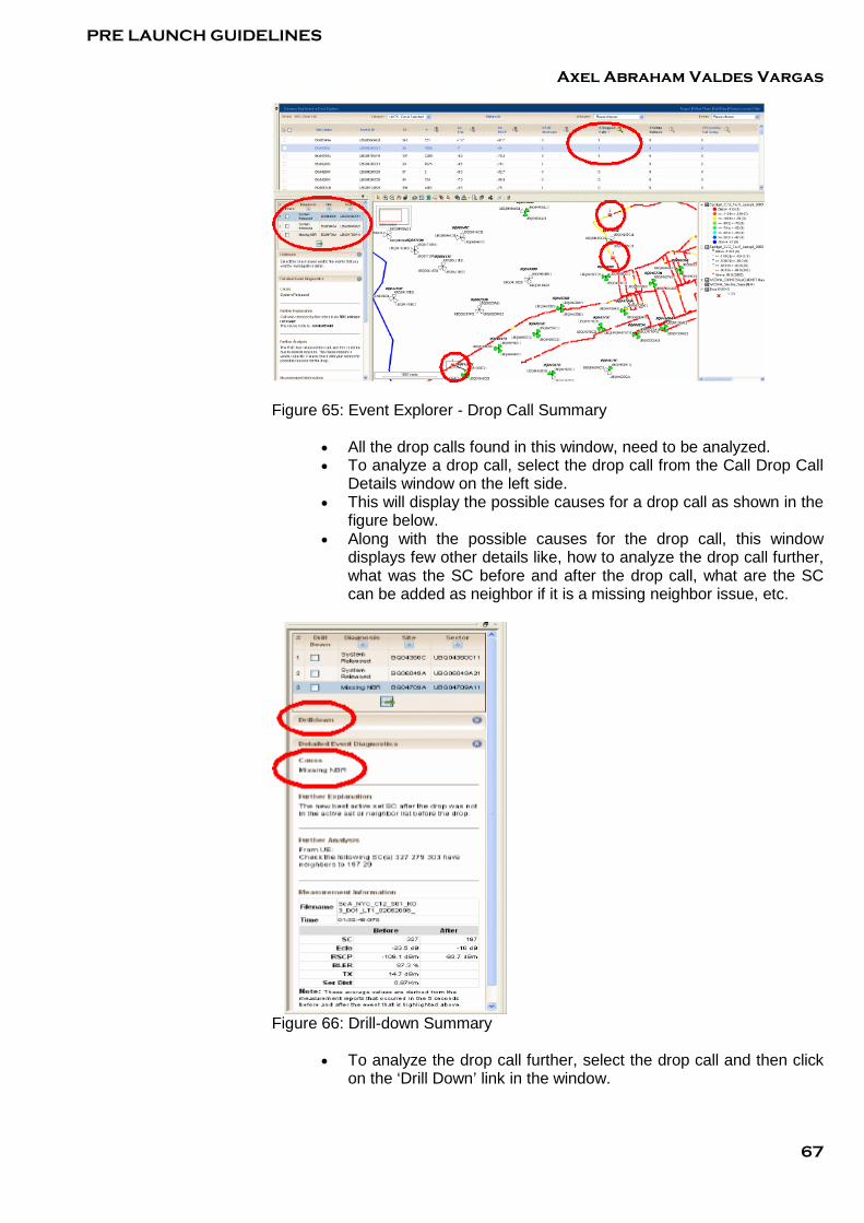
PRE LAUNCH GUIDELINES
Axel Abraham Valdes Vargas
67
Figure 65: Event Explorer - Drop Call Summary
• All the drop calls found in this window, need to be analyzed. • To analyze a drop call, select the drop call from the Call Drop Call
Details window on the left side. • This will display the possible causes for a drop call as shown in the
figure below. • Along with the possible causes for the drop call, this window
displays few other details like, how to analyze the drop call further, what was the SC before and after the drop call, what are the SC can be added as neighbor if it is a missing neighbor issue, etc.
Figure 66: Drill-down Summary
• To analyze the drop call further, select the drop call and then click on the ‘Drill Down’ link in the window.

PRE LAUNCH GUIDELINES
Axel Abraham Valdes Vargas
68
• The time before & after the drop call can be selected. Alternatively, the entire file can be loaded.
• This opens an another window shown below Figure 67 with all details about the drop call including Layer 3 messages before and after drop call based on the time chosen, Drive Route map, Drop Location, Coverage Conditions during the time window chosen, etc.
Figure 67: Spotlight Drop Call Analysis 4.9. Packet Session Data Analysis Low throughput can be caused by simple RF issues as well as complex end to end system issues. It is important that during optimization, low throughput be identified, analyzed, and resolved where possible with irresolvable problems escalated to E2E support. As the packet switched service is a best effort service, with lower priority than circuit switched services the user throughput is often highly variable. Packet data is handled using common channels, dedicated channels and shared channels, each offering different capability and throughput. Which of these is assigned is dependent on UE capability, data volume, RF conditions, available resources (hardware, transmission, code etc). The three states used for data transfer are listed below:
1. Using common channels : FACH/RACH* 2. Using R99 DCH: 64 or 128 or 384 / 64 or 128 or 384 3. Using Shared Channels: HS / 64 or 128 or 384
* FACH/RACH analysis is not included separately in this document, however is mentioned as part of the R99 PS DCH section. The following flowchart describes the process for investigating throughput issues.
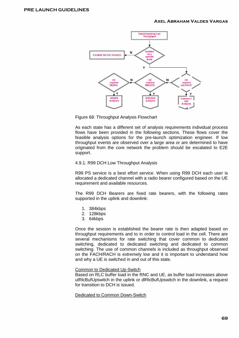
PRE LAUNCH GUIDELINES
Axel Abraham Valdes Vargas
69
Figure 68: Throughput Analysis Flowchart As each state has a different set of analysis requirements individual process flows have been provided in the following sections. These flows cover the feasible analysis options for the pre-launch optimization engineer. If low throughput events are observed over a large area or are determined to have originated from the core network the problem should be escalated to E2E support. 4.9.1. R99 DCH Low Throughput Analysis R99 PS service is a best effort service. When using R99 DCH each user is allocated a dedicated channel with a radio bearer configured based on the UE requirement and available resources. The R99 DCH Bearers are fixed rate bearers, with the following rates supported in the uplink and downlink:
1. 384kbps 2. 128kbps 3. 64kbps
Once the session is established the bearer rate is then adapted based on throughput requirements and to in order to control load in the cell. There are several mechanisms for rate switching that cover common to dedicated switching, dedicated to dedicated switching and dedicated to common switching. The use of common channels is included as throughput observed on the FACH/RACH is extremely low and it is important to understand how and why a UE is switched in and out of this state. Common to Dedicated Up-Switch Based on RLC buffer load in the RNC and UE, as buffer load increases above ulRlcBufUpswitch in the uplink or dlRlcBufUpswitch in the downlink, a request for transition to DCH is issued. Dedicated to Common Down-Switch

PRE LAUNCH GUIDELINES
Axel Abraham Valdes Vargas
70
Based on throughput in the uplink and downlink as measured by the SRNC, as the throughput in both uplink and downlink falls below downswitchThreshold and remains below for a period of time as defined by downswitchTimer the UE will be transitioned from a dedicated state to a common state (FACH/RACH). Dedicated to Dedicated Down-Switch Based on coverage and/or throughput. Coverage assessment is based on the transmitted code power, where the transmitted code power exceeds the threshold, defined by downswitchPwrMargin, for a period of time defined by coverageTimer, a down-switch to the next lowest rate will be requested. This only applies to bearer rates of 128k and 384k. Throughput based assessment is performed on the uplink and downlink separately. Thresholds are defined in the uplink by ulDownswitchBandwidthMargin and the downlink by dlDownswitchBandwidthMargin if these are met for a period of time defined by dlThroughputDownswitchTimer and ulThroughputDownswitchTimer a down-switch to the next lowest uplink or downlink bearer is requested. Dedicated to Dedicated Up-Switch Throughput based. Uplink and downlink throughput is monitored separately and an up-switch request sent where the throughput increases above the threshold for uplink or downlink as defined by bandwidthMargin and bandwidthMarginUl; for downlink requests the transmitted code power is below the upswitchPwrMargin; QoS parameters allow the higher rate; and after a throughput based down-switch the throughput has fallen below dlThroughputAllowUpswitchThresh or ulThroughputAllowUpswitchThresh to prevent ping pong rate switching. From these basic descriptions of the channel switching function it is clear that the biggest potential contributors to low throughput are coverage, application server and system resources. When considering the unloaded case coverage and the application server are the primary considerations and as load increases user experience becomes a trade-off between user throughput and system throughput. The following section details how to identify areas of low R99 DCH throughput using Actix. 4.9.2.Using Actix To Identify Low R99 Throughput R99 throughput is not summarized by spotlight into a category with an associated workspace, and therefore the engineer must make use of analysis techniques using the classic Actix functionality. The following sections detail how to access the required attributes to undertake throughput analysis. The most efficient way to evaluate R99 throughput is graphically, either charted or plotted on a map. This provides the engineer with a easy reference for problem areas. Note: Currently with no high level binning of application throughput, log files must be loaded and super streamed together for this analysis. The main attributes that should be viewed are:

PRE LAUNCH GUIDELINES
Axel Abraham Valdes Vargas
71
1. Mapping – Application throughput (Figure 69) 2. Charting – Application throughput, RLC PDU throughput, and
Cumulative Rx Bytes (Figure 70)
Figure 69: Application Throughput
Figure 70: Application Throughput Chart From Figure 69 it is evident that the area enclosed within the dotted red circle is an area of low throughput (throughput rarely exceeding 32kbps) that requires investigation. Similarly from Figure 70 sessions with low throughput are shown enclosed within dotted red ovals. As maps and charts are event synchronized, clicking on a point in the area will align all other open forms for analysis.

PRE LAUNCH GUIDELINES
Axel Abraham Valdes Vargas
72
Once areas of low throughput are identified the following attributes and forms can then be used to assist in the analysis.
1. Uu_ActiveSet_EcNo_0 – best server Ec/No plotted or charted provides a measure of the quality of coverage the Ue is experiencing, areas with poor Ec/No can cause low throughput where the transmitted code power approaches the allowed maximum. Typically the better the Ec/No the higher the supported bearer rates.
2. Uu_TrCh_DownlinkBlerAgg – Transport Channel Block Error rate aggregated over the control and traffic channels. This attribute indicates the level of errors introduced over the air interface.
3. UE_TxPow – UE transmitted power, useful indicator of uplink coverage.
4. Uu_PS_AllocatedRate – allocated bearer, updated at each rate or bearer switch.
Attributes a), b), c) and d) are accessed from the attribute explorer as shown in Figure 71.
Figure 71: Attribute Locations The following forms are recommended to support analysis:
1. Protocol Stack Browser
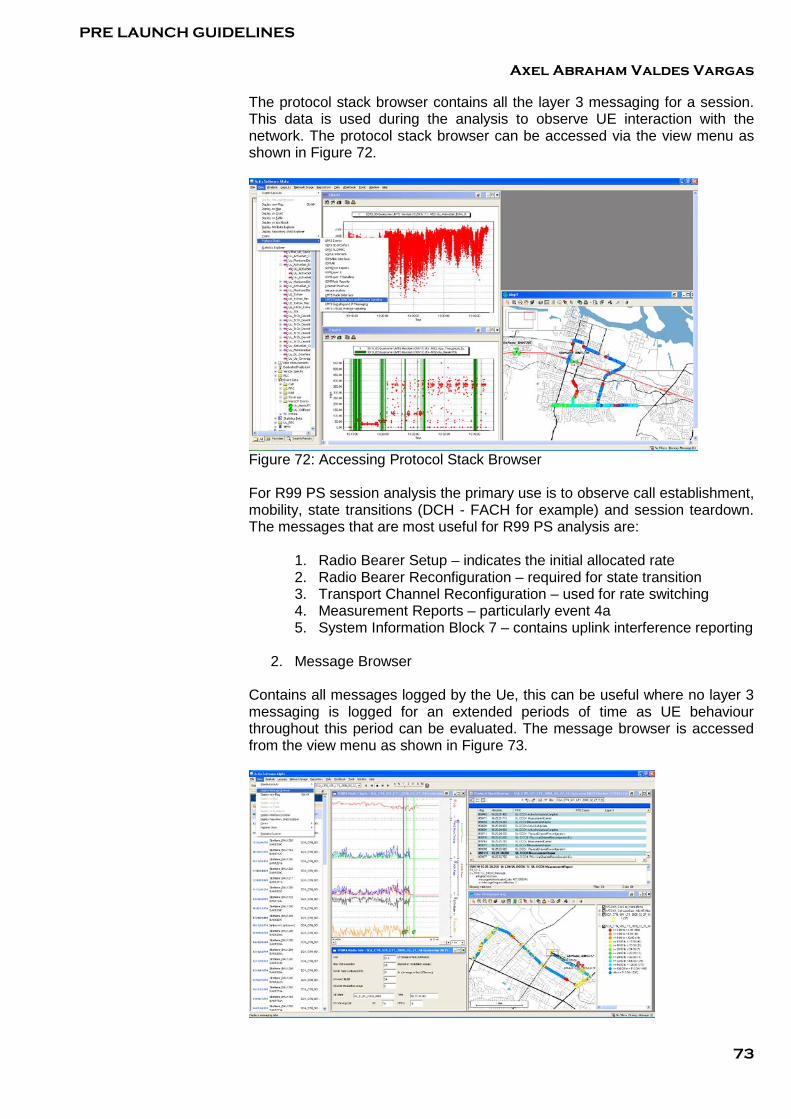
PRE LAUNCH GUIDELINES
Axel Abraham Valdes Vargas
73
The protocol stack browser contains all the layer 3 messaging for a session. This data is used during the analysis to observe UE interaction with the network. The protocol stack browser can be accessed via the view menu as shown in Figure 72.
Figure 72: Accessing Protocol Stack Browser For R99 PS session analysis the primary use is to observe call establishment, mobility, state transitions (DCH - FACH for example) and session teardown. The messages that are most useful for R99 PS analysis are:
1. Radio Bearer Setup – indicates the initial allocated rate 2. Radio Bearer Reconfiguration – required for state transition 3. Transport Channel Reconfiguration – used for rate switching 4. Measurement Reports – particularly event 4a 5. System Information Block 7 – contains uplink interference reporting
2. Message Browser
Contains all messages logged by the Ue, this can be useful where no layer 3 messaging is logged for an extended periods of time as UE behaviour throughout this period can be evaluated. The message browser is accessed from the view menu as shown in Figure 73.

PRE LAUNCH GUIDELINES
Axel Abraham Valdes Vargas
74
Figure 73: Accessing Message Browser
3. UMTS Missing Neighbors Form This form contains active set and monitored set scrambling codes with RSCP and Ec/No as seen by the Ue as well as scanned scrambling codes for the same time instant. The form is accessed from the view menu as shown in Figure 74 and shown in Figure 75. This form offers a fast way to identify missing neighbors that contribute to poor RF as observed by the UE.
Figure 74: Accessing UMTS Missing Neighbors
Figure 75: UMTS Missing Neighbors 4.9.3.Using Actix To Analyze Low R99 Throughput The following workflow describes a process for investigating low throughput in R99.

PRE LAUNCH GUIDELINES
Axel Abraham Valdes Vargas
75
Figure 76: Low Throughput Investigation Flowchart Each cause shown in the flowchart above is discussed below with recommended solutions: 1. Prolonged Cell_FACH As the transitions to and from FACH/RACH are determined by throughput, when a UE stays in cell FACH state for a prolonged period of time it is probable that either the application server is failing to provide sufficient data to maintain the required throughput for a dedicated channel or that there are insufficient resources to allocate a DCH. This is particularly evident where there is no apparent coverage or interference problem and the network is unloaded.
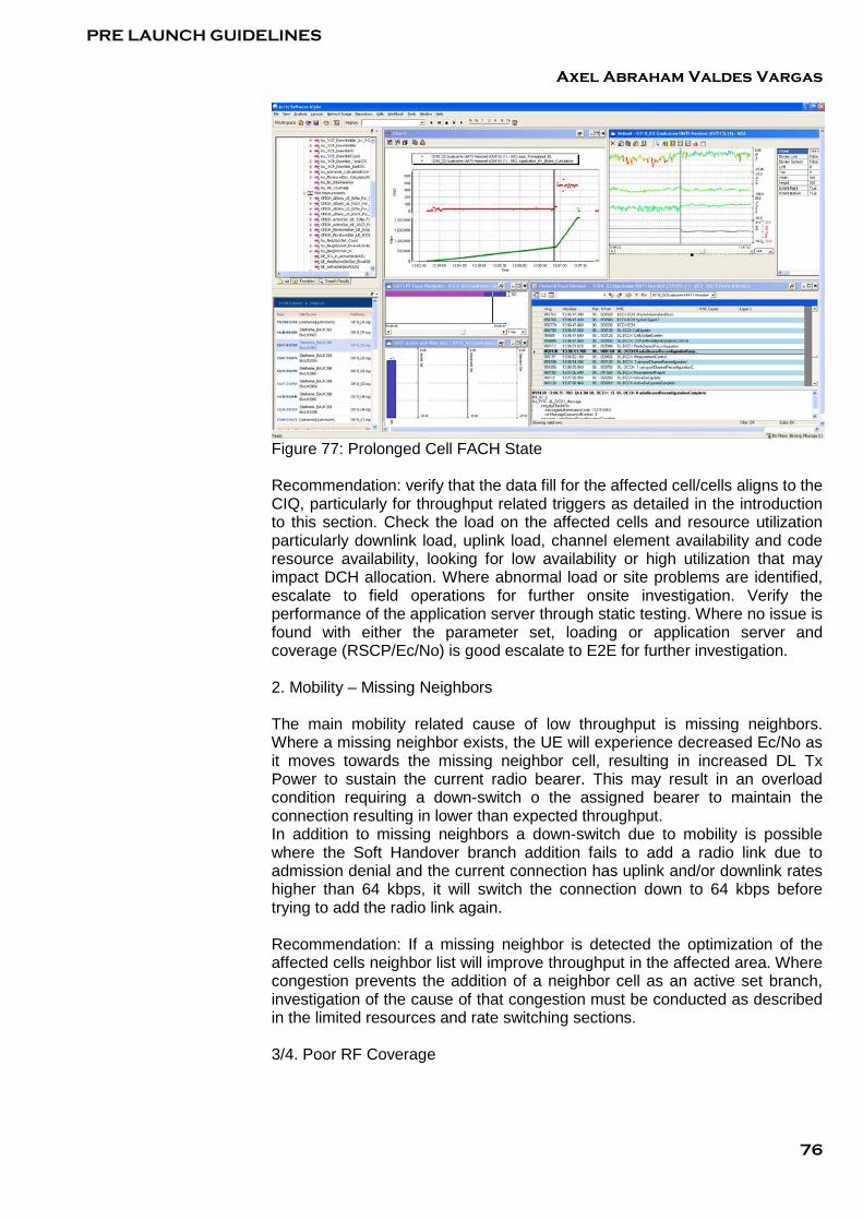
PRE LAUNCH GUIDELINES
Axel Abraham Valdes Vargas
76
Figure 77: Prolonged Cell FACH State Recommendation: verify that the data fill for the affected cell/cells aligns to the CIQ, particularly for throughput related triggers as detailed in the introduction to this section. Check the load on the affected cells and resource utilization particularly downlink load, uplink load, channel element availability and code resource availability, looking for low availability or high utilization that may impact DCH allocation. Where abnormal load or site problems are identified, escalate to field operations for further onsite investigation. Verify the performance of the application server through static testing. Where no issue is found with either the parameter set, loading or application server and coverage (RSCP/Ec/No) is good escalate to E2E for further investigation. 2. Mobility – Missing Neighbors The main mobility related cause of low throughput is missing neighbors. Where a missing neighbor exists, the UE will experience decreased Ec/No as it moves towards the missing neighbor cell, resulting in increased DL Tx Power to sustain the current radio bearer. This may result in an overload condition requiring a down-switch o the assigned bearer to maintain the connection resulting in lower than expected throughput. In addition to missing neighbors a down-switch due to mobility is possible where the Soft Handover branch addition fails to add a radio link due to admission denial and the current connection has uplink and/or downlink rates higher than 64 kbps, it will switch the connection down to 64 kbps before trying to add the radio link again. Recommendation: If a missing neighbor is detected the optimization of the affected cells neighbor list will improve throughput in the affected area. Where congestion prevents the addition of a neighbor cell as an active set branch, investigation of the cause of that congestion must be conducted as described in the limited resources and rate switching sections. 3/4. Poor RF Coverage

PRE LAUNCH GUIDELINES
Axel Abraham Valdes Vargas
77
This section covers 2 blocks in the work flow (RSCP, Ec/No). While it is not possible to accurately identify an “RF threshold” for the assignment of a particular bearer rate, it can be stated arbitrarily that:
1. When a UE is experiencing good RF conditions (Ec/No > -12dB) that a higher rate bearer can be assigned than when a UE is in poor RF conditions (Ec/No < -12dB).
2. When considering RSCP, a UE reporting a RSCP level approaching “cell edge” (RSCP < -95dBm) is unlikely to be assigned a high rate bearer as the power required to overcome the path loss is likely to be beyond the maximum defined code power.
The actual rate assignment is based on RNC RRM algorithms that use reported information from the UE along with inputs from many other RRM functions that the analysis engineer has no immediate visibility of. Figure 78 shows an example of the impact poor RF can have on PS throughput. In this example 64kbps and FACH are assigned in poor RF and as Ec/No improves 384kbps bearers are assigned more readily.
Figure 78: Poor Coverage Impact on Throughput Recommendation: where low throughput is observed as a result of poor uplink or downlink coverage, optimization of downlink coverage to improve dominance through either increasing the RSCP of a likely best server or by reducing the interference caused by unwanted servers will result in improved throughput over the area. 5. High BLER High BLER due to errors introduced in the air interface can be caused by a poor RF environment as well as external interference and a loss of synchronization in good RF. In order to recover an erroneously received packets, AM RLC retransmits these packets. The higher the BLER the more retransmissions required and the lower the resulting application throughput. RLC retransmissions can be observed in the RLC attributes accessed via the attribute explorer. When very high BLER is prolonged eventually the session will drop to idle.

PRE LAUNCH GUIDELINES
Axel Abraham Valdes Vargas
78
Recommendation: where consistently high BLER is encountered prior to a drop to idle, it is likely that synchronization has been lost, this is often seen immediately following an active set update. If the connection is lost the resulting layer 3 cell update messaging will provide cause information. If not related to a synchronization issue and a contributing interferer cell cannot be identified it is possible that an external interferer is present in the area and should be escalated to a field technician for investigation. 6. Rate Switching and RRM Functions The Rate Switching evaluation is based on two conditions, user activity and load. User activity is measured in terms of either the channel throughput or RLC buffer load. Load is measured in terms of downlink code power. When there is low or no user activity, a down-switch is requested. When on CELL_DCH, the detection is based on throughput measurement and the connection will be switched down either to a lower rate on CELL_DCH or to CELL_FACH depending on throughput level. The Load Triggered Down-Switch Evaluation algorithm monitors whether a switch to a lower rate dedicated channel is required due downlink load (Total DL Tx Power). Where the required DL power to sustain a current RL exceeds the available power the user will be down-switched to a lower rate bearer, this can occur as a result of coverage limitations or the load created by other users in the cell. In the event that the cell is in an overload state, the load control algorithm will prevent new session additions and target the highest rate users for downgrade until the overload situation is resolved. In addition to the load control algorithm maintaining a session by adjusting the bearer to accommodate the available load, admission control and resource management algorithms are responsible for admitting new sessions to the cell and maintaining code and hardware resource. As the PS service has a lower priority than voice, it is possible that a PS user will be downgraded or dropped in favor of a new CS admission if resources are limited. Figure 79 shows a coverage triggered down-switch from a 384kbps bearer to a 128kbps bearer, then 64kbps with the session finally dropping to idle.
Figure 79: Coverage Triggered Down-switch

PRE LAUNCH GUIDELINES
Axel Abraham Valdes Vargas
79
Recommendation: Where it is evident that coverage is the trigger for down-switching (indicated by an associated decline in Ec/No / RSCP and or increase in UE Tx Power), optimization of downlink coverage to improve dominance through either increasing the RSCP of a likely best server or by reducing the interference caused by unwanted servers will result in improved throughput over the area. In that event that a down-switch or connection release cannot be explained by a RF related cause, it is necessary to investigate the RNC counters for abnormal load, rate switching behavior, and hardware congestion, if found escalation to the field technician for resolution is required. The specific counters for Nokia are detailed below. Ericsson’s counters will be added at a later date. Nokia: Load - M1000C14 - M1000C23, M1000C230, M100C231 Hardware Congestion – M5001C0, M5001C1, M5001C2 Code Congestion – M1000C77, M100C78, M1000C79 Rate Switching - M1000C142, M1000C145, M1000C146, M1000C147, M1000C148, M1000C154, M1000C157, M1000C158, M1000C159, M1000C160, M1000C166 User activity down-switching is a product of the application rather than RAN, where a low rate DCH or CELL_FACH is assigned in good RF with low BLER it is probable that the experienced throughput is the result of an application issue. In the event that a user is being constantly switched between bearer rates or states it is likely that there is a parameter issue. Confirm that the assigned parameter set aligns to the CIQ. 4.9.4. HSDPA Low Throughput Analysis HSDPA offers users enhanced data rates and improved latency over traditional R99 bearers, with throughputs as high as 14.4Mbps achievable. With HSDPA, users make use of the DSCH (comprising several sf16 codes) rather than the DCH for data transfer in the downlink, the scheduling of user data is performed by the a new MAC entity (MAC-hs) in the NodeB rather than the RNC and fast HARQ is used to minimize RLC retransmissions caused by errors introduced over the air interface. The commercial HSDPA configuration is as follows:
• Enabling – All cells • Minimum Allocated Power – Depends on Ericsson/Nokia parameter
settings • Codes – 5 • Modulation – QPSK and 16QAM • Scheduler – Proportional Fair
Assuming a UE class that allows sequential TTI scheduling, this configuration allows for a maximum throughput for a single user of 3.6 Mbps.

PRE LAUNCH GUIDELINES
Axel Abraham Valdes Vargas
80
The definition of a low HSDPA throughput event in Actix is: Raw Throughput: (Physical Layer throughput) – Raw HSDPA throughput lower than 400kbps occurs for longer than 3 seconds. Net Throughput: (MAC-hs layer throughput) – MAC-hs layer HSDPA throughput lower than 300kbps occurs for longer than 3 seconds. As the individual low throughput events will be too numerous to investigate, it is necessary to identify and analyze throughput related to a common thread, eg. An area of limited coverage causing low throughput or low throughput unique to a specific cell or site. The following section describes how to locate low throughput events and analyze these events using Actix Spotlight. 4.9.5.Using Actix To Identify Low HSDPA Throughput HSPDA throughput is summarized by spotlight into a category with an associated workspace. The following sections detail how to access this workspace and associated attributes that can be used to assist in analysis. 4.9.5.1.Event Explorer Using spotlight it is possible to identify specific instances of low throughput for an HSDPA service. This is done by selecting the HSDPA Throughput option from the category drop down in the event explorer as shown in Figure 80.
Figure 80: Selecting HSDPA Throughput Event Category
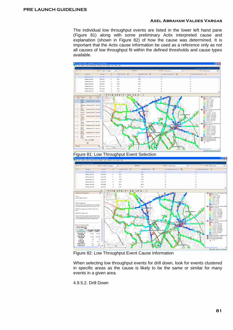
PRE LAUNCH GUIDELINES
Axel Abraham Valdes Vargas
81
The individual low throughput events are listed in the lower left hand pane (Figure 81) along with some preliminary Actix interpreted cause and explanation (shown in Figure 82) of how the cause was determined. It is important that the Actix cause information be used as a reference only as not all causes of low throughput fit within the defined thresholds and cause types available.
Figure 81: Low Throughput Event Selection
Figure 82: Low Throughput Event Cause Information When selecting low throughput events for drill down, look for events clustered in specific areas as the cause is likely to be the same or similar for many events in a given area. 4.9.5.2. Drill Down
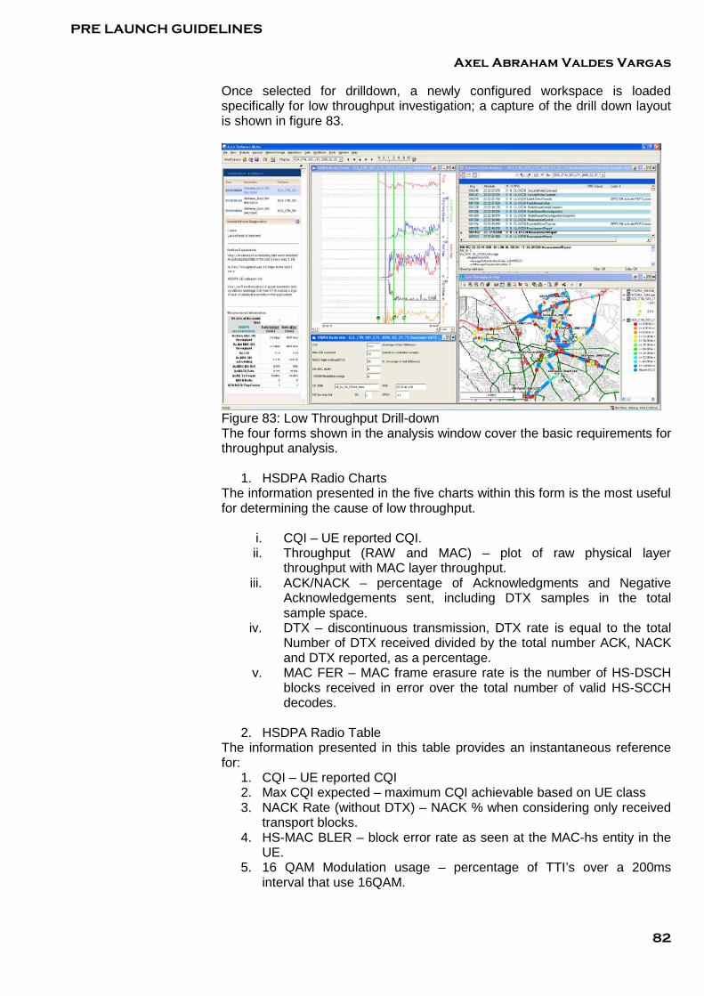
PRE LAUNCH GUIDELINES
Axel Abraham Valdes Vargas
82
Once selected for drilldown, a newly configured workspace is loaded specifically for low throughput investigation; a capture of the drill down layout is shown in figure 83.
Figure 83: Low Throughput Drill-down The four forms shown in the analysis window cover the basic requirements for throughput analysis.
1. HSDPA Radio Charts The information presented in the five charts within this form is the most useful for determining the cause of low throughput.
i. CQI – UE reported CQI. ii. Throughput (RAW and MAC) – plot of raw physical layer
throughput with MAC layer throughput. iii. ACK/NACK – percentage of Acknowledgments and Negative
Acknowledgements sent, including DTX samples in the total sample space.
iv. DTX – discontinuous transmission, DTX rate is equal to the total Number of DTX received divided by the total number ACK, NACK and DTX reported, as a percentage.
v. MAC FER – MAC frame erasure rate is the number of HS-DSCH blocks received in error over the total number of valid HS-SCCH decodes.
2. HSDPA Radio Table
The information presented in this table provides an instantaneous reference for:
1. CQI – UE reported CQI 2. Max CQI expected – maximum CQI achievable based on UE class 3. NACK Rate (without DTX) – NACK % when considering only received
transport blocks. 4. HS-MAC BLER – block error rate as seen at the MAC-hs entity in the
UE. 5. 16 QAM Modulation usage – percentage of TTI’s over a 200ms
interval that use 16QAM.

PRE LAUNCH GUIDELINES
Axel Abraham Valdes Vargas
83
6. UE State – indication of the current UE state, useful to check if UE is in HS-DSCH state at the time of a low throughput event.
7. Time – timestamp of the selected event or point in the file. 8. HS Serving Cell
i. SC – scrambling code of the active set cell transmitting the HS-PDSCH
ii. Ec/No – current Ec/No of the serving scrambling code
3. Protocol Stack Browser The protocol stack browser contains all the layer 3 messaging for a session. This data is used during the analysis to observe UE interaction with the network. For HSDPA the primary use is to observe call establishment, mobility, state transitions (HSDPA -> DCH for example) and session teardown. The messages that are most useful for HSDPA analysis are:
1. Radio Bearer Setup – indicates whether or not HSDPA is allocated 2. Radio Bearer Reconfiguration – required for state transition and ISHO
procedures. 3. Physical Channel Reconfiguration – used for HS-PDSCH switching
(best server change) 4. Measurement Reports – particularly e1d triggers
4. Map
When first opened the map displays graphically the application throughput, and low throughput events can be observed spatially this way. It is possible to display any map based attribute on this map using the attribute explorer to support analysis as required. (eg. Ec/No, RSCP, average CQI etc.) 4.9.5.3.Additional Attributes While the forms and charts presented in the basic workspace give a useful insight into the session performance there are several other attributes that can be displayed or referenced to assist in analysis. An indication of throughput at various layers in the protocol stack provides useful information on the cause of low throughput. Actix is able to extract a measure of throughput at several points in the protocol stack, the main lower layer throughput attributes that should be referenced during the analysis are listed below:
1. Uu_HSDPA_PayloadRate_L1 – total L1 throughput, includes retransmissions and erroneous packets
2. Uu_HSDPA_Throughput_L1 – HARQ level throughput, excluding transport blocks received in error
3. Uu_HSDPA_Throughput_MAC – HARQ level throughput, excluding transport blocks received in error and multiple reception of the error free transport blocks.
The HSDPA Radio Charts – Throughput plots. To view the additional throughput metric it is necessary to use the attribute explorer as shown in Figure 84 and Figure 85.

PRE LAUNCH GUIDELINES
Axel Abraham Valdes Vargas
84
Figure 84: Locating Attribute Explorer
Figure 85: Location of Specific HSDPA Throughput Attributes The throughout attributes mentioned above are measured at L1 and MAC-hs layers and relate to the throughput between the Ue and the NodeB, these attributes are not necessarily indicative of the throughput experienced by the user. To view the resulting user or application layer throughput and session progress the following attributes should be referenced:
1. Application Throughput DL – user realized throughput at the application layer.
2. Cumulative Rx Bytes – shows the cumulative application layer bytes downloaded over the duration of a session.
These can be found using the attribute explorer as shown in Figure 86.

PRE LAUNCH GUIDELINES
Axel Abraham Valdes Vargas
85
Figure 86: Location of Specific Application Throughput Attributes When these attributes are plotted together on the same chart it is possible to quickly reference areas of low throughput, and session issues for the loaded log file. Figure 87 shows an example.
Figure 87: Physical Application Layer Throughput & Received Cumulative Bytes The sessions shown in this example are a good reference; the first session shows a download within a variable RF environment, throughput declines throughout the session which takes a long time to complete; the second session suffers low throughput and drops prior to completion (cumulative Rx bytes does not reach 5MB); the third and fourth show near ideal FTP download sessions with largely stable throughput and fast completion; the final session shown is another failure example where very little data is transferred prior to drop.
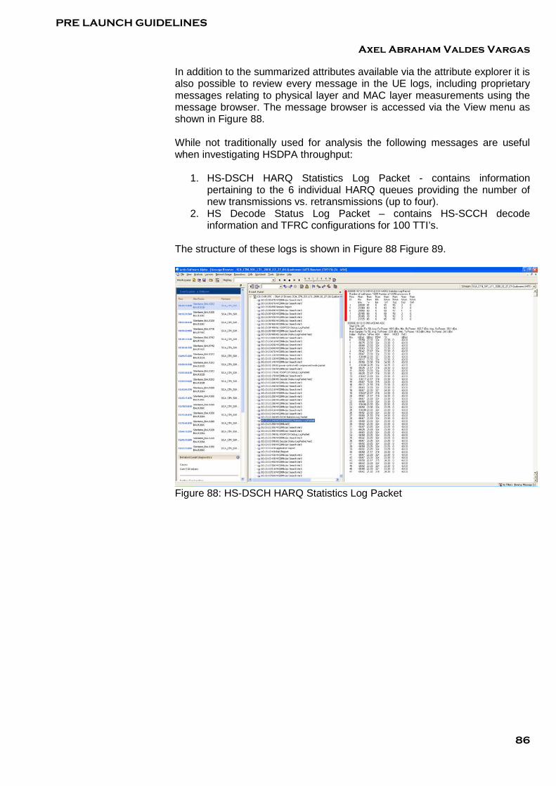
PRE LAUNCH GUIDELINES
Axel Abraham Valdes Vargas
86
In addition to the summarized attributes available via the attribute explorer it is also possible to review every message in the UE logs, including proprietary messages relating to physical layer and MAC layer measurements using the message browser. The message browser is accessed via the View menu as shown in Figure 88. While not traditionally used for analysis the following messages are useful when investigating HSDPA throughput:
1. HS-DSCH HARQ Statistics Log Packet - contains information pertaining to the 6 individual HARQ queues providing the number of new transmissions vs. retransmissions (up to four).
2. HS Decode Status Log Packet – contains HS-SCCH decode information and TFRC configurations for 100 TTI’s.
The structure of these logs is shown in Figure 88 Figure 89.
Figure 88: HS-DSCH HARQ Statistics Log Packet

PRE LAUNCH GUIDELINES
Axel Abraham Valdes Vargas
87
Figure 89: HS Decode Status Log Packet Example 4.9.6. Using Actix To Analyze Low HSDPA Throughput The following workflow describes a process for investigating low throughput in HSDPA

PRE LAUNCH GUIDELINES
Axel Abraham Valdes Vargas
88
Figure 90: Low HSDPA Throughput Analysis Flowchart Each stage of analysis shown in the flowchart above is discussed below with recommended solutions: 1. Beginning of the Session - TCP Slow Start Immediately following PDP Activation Accepted the application throughput begins to ramp up slowly towards the achievable rate. This is due to TCP congestion control algorithms and is called TCP slow start. This will result in lower than expected throughput over the first few seconds of a HSDPA session, this is normal application behavior and should not be considered as a low throughput problem. Figure 91 shows an example of TCP slow start, the beginning of the session is indicated by a red dashed oval.
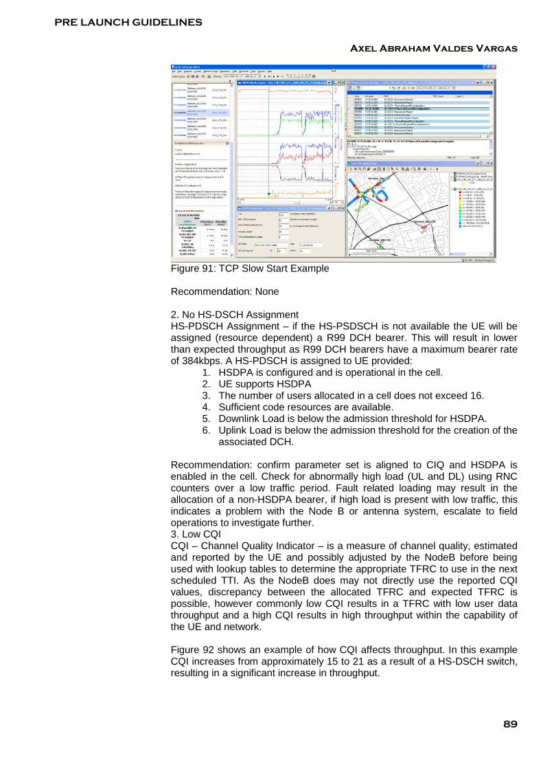
PRE LAUNCH GUIDELINES
Axel Abraham Valdes Vargas
89
Figure 91: TCP Slow Start Example Recommendation: None 2. No HS-DSCH Assignment HS-PDSCH Assignment – if the HS-PSDSCH is not available the UE will be assigned (resource dependent) a R99 DCH bearer. This will result in lower than expected throughput as R99 DCH bearers have a maximum bearer rate of 384kbps. A HS-PDSCH is assigned to UE provided:
1. HSDPA is configured and is operational in the cell. 2. UE supports HSDPA 3. The number of users allocated in a cell does not exceed 16. 4. Sufficient code resources are available. 5. Downlink Load is below the admission threshold for HSDPA. 6. Uplink Load is below the admission threshold for the creation of the
associated DCH. Recommendation: confirm parameter set is aligned to CIQ and HSDPA is enabled in the cell. Check for abnormally high load (UL and DL) using RNC counters over a low traffic period. Fault related loading may result in the allocation of a non-HSDPA bearer, if high load is present with low traffic, this indicates a problem with the Node B or antenna system, escalate to field operations to investigate further. 3. Low CQI CQI – Channel Quality Indicator – is a measure of channel quality, estimated and reported by the UE and possibly adjusted by the NodeB before being used with lookup tables to determine the appropriate TFRC to use in the next scheduled TTI. As the NodeB does may not directly use the reported CQI values, discrepancy between the allocated TFRC and expected TFRC is possible, however commonly low CQI results in a TFRC with low user data throughput and a high CQI results in high throughput within the capability of the UE and network. Figure 92 shows an example of how CQI affects throughput. In this example CQI increases from approximately 15 to 21 as a result of a HS-DSCH switch, resulting in a significant increase in throughput.
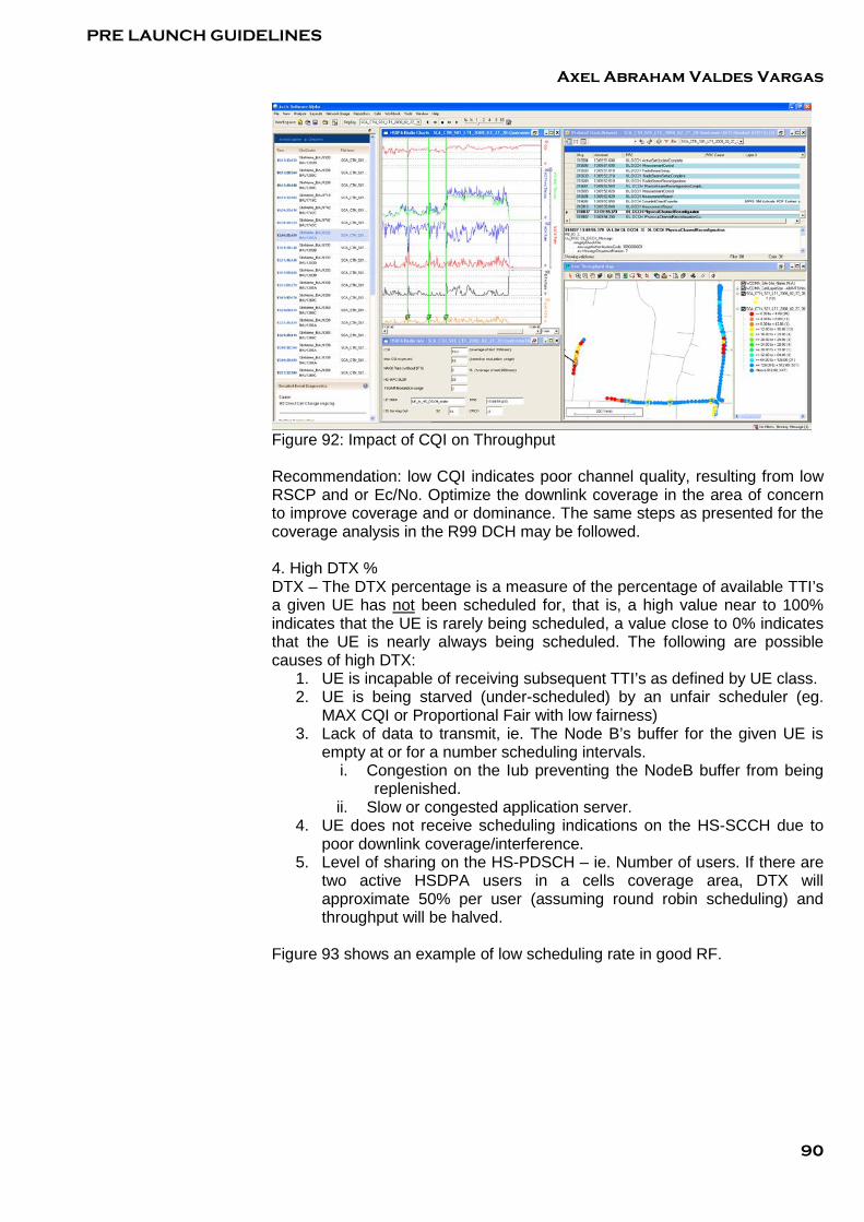
PRE LAUNCH GUIDELINES
Axel Abraham Valdes Vargas
90
Figure 92: Impact of CQI on Throughput Recommendation: low CQI indicates poor channel quality, resulting from low RSCP and or Ec/No. Optimize the downlink coverage in the area of concern to improve coverage and or dominance. The same steps as presented for the coverage analysis in the R99 DCH may be followed. 4. High DTX % DTX – The DTX percentage is a measure of the percentage of available TTI’s a given UE has not been scheduled for, that is, a high value near to 100% indicates that the UE is rarely being scheduled, a value close to 0% indicates that the UE is nearly always being scheduled. The following are possible causes of high DTX:
1. UE is incapable of receiving subsequent TTI’s as defined by UE class. 2. UE is being starved (under-scheduled) by an unfair scheduler (eg.
MAX CQI or Proportional Fair with low fairness) 3. Lack of data to transmit, ie. The Node B’s buffer for the given UE is
empty at or for a number scheduling intervals. i. Congestion on the Iub preventing the NodeB buffer from being
replenished. ii. Slow or congested application server.
4. UE does not receive scheduling indications on the HS-SCCH due to poor downlink coverage/interference.
5. Level of sharing on the HS-PDSCH – ie. Number of users. If there are two active HSDPA users in a cells coverage area, DTX will approximate 50% per user (assuming round robin scheduling) and throughput will be halved.
Figure 93 shows an example of low scheduling rate in good RF.

PRE LAUNCH GUIDELINES
Axel Abraham Valdes Vargas
91
Figure 93: High DTX in Good RF causing Low Throughput Recommendation: Where a consistently high DTX rate is observed in good RF across a wide area of a cells footprint it is probable that there is a hardware issue at the NodeB, this should be escalated to field operations to investigate further on site. It may be necessary to re-commission HSDPA on the site. Where high DTX is observed sporadically throughout a session it is probable that there is insufficient data in the buffers for the UE to be continuously scheduled, this can be due to congestion in the Iub or an under-performing FTP server. Verify the performance of the FTP server with static testing and check RNC counters for Iub congestion events. 5. High NACK % ACK vs. NACK – For every TTI in which a UE is scheduled to receive data, the UE will respond by sending an ACK or NACK depending on whether or not the transmission was correctly received or not. (Note that if the UE does not receive the scheduling information on the HS-SCCH, no HARQ response is sent (DTX)). As each NACK requires a physical layer retransmission of the transport block a high percentage of NACK’s can cause low throughput. This is only true where Uu_ HSDPA_Throughput_MAC decreases as a result. It is feasible that the retransmissions can be absorbed with a higher Uu_HSDPA_Payload_L1 rate. A consistently high NACK % indicates that the link adaptation algorithm is not able to adequately track the radio environment, this can result from:
1. NodeB or ATS problem – when a site or cell is consistently showing high NACK % for all sessions on the site / cell, this can indicate a problem with the NodeB configuration or antenna system.
2. UE is over reporting CQI – less likely scenario as CQI reporting accuracy is standardized. There is still a possibility that a UE under performs in this area however and this will cause a reduction in system throughput when more than one user is active in a cell.

PRE LAUNCH GUIDELINES
Axel Abraham Valdes Vargas
92
Figure 94 shows an example of consistently high NACK % in good RF.
Figure 94: High NACK Impacting User Throughput Recommendation: If present consistently from a given time to the end of the drive test verify the UE performance in a static test to rule this out as a cause. If the problem is observed on all HSDPA connections in a particular cell escalate to a field technician to verify the antenna system and antenna system settings in the NodeB for the affected cell/cells, and to confirm the HSDPA commissioning parameters, these should align to the CIQ data. To overcome UE CQI over-reporting it is possible to use the Ericsson RBS cqiAdjustmentOn parameter. This activates the NodeB CQI adjustment algorithm which targets a NACK% of 10%. Warning – this can result is reduced user throughput in good RF. This parameter should not be changed without prior approval. 6. Mobility Mobility – while mobility should no longer severely impact user throughput (with the use of A-DCH SHO and HS-PDSCH switching), it is possible that incorrectly set mobility parameters for HSDPA may cause delayed HS-PDSCH switching, as a result the HS-PDSCH may not always be on the best server and experience lower than achievable throughput. In addition constant switching or ping pong switching can cause reduced application throughput as data in the source NodeB buffer is discarded and recovered in the target cell through higher layer retransmissions (RLC). Recommendation: verify e1d trigger parameter alignment, optimize SHO area by creating single cell dominance in the affected area. 5. Market Level Optimization

PRE LAUNCH GUIDELINES
Axel Abraham Valdes Vargas
93
To perform Market Level Optimization, a Market is divided into several sub-markets. Each sub market can be grouped into 250 300 sites depending on the site density, morphology and expected subscriber’s mobility. This phase is reached once all clusters in the market have been accepted. 5.1.Objective The objective of market level optimization is to optimize IRAT performance at the market coverage boundaries as well as collecting data that reflects a user experience by allowing the UEs to perform IRAT Handovers. In addition, data is collected to provide a comparison against GSM metrics. Following are the required KPIs to be met at the market level. At this stage, it is anticipated that a low amount of changes will be needed with the bulk of Optimization changes having been performed at the Cluster level.
Table 8: Market Acceptance KPIs 5.2.Process Flow 5.2.1.Market Loaded Optimization The flowchart of Market Loaded Optimization is shown below. There will be 2 drive tests for this phase with any further drives requiring the UMTS PMO approval. Setup 1 (IRAT Boundary Test) will have the drive test initiated from within the UMTS coverage area and drive towards the edge o the network until the CS & PS calls perform IRAT handover to GSM or drop calls occur. Setup 2(Mobile Test) will be setup to allow the UMTS UEs to perform IRAT within the UMTS coverage areas. This is to reflect the comparative experience that a user would face whilst travelling through the UMTS coverage area. Setup 2 (Stationary Test) will only occur if stationary testing that was initiated during Cluster Optimization was not completed.
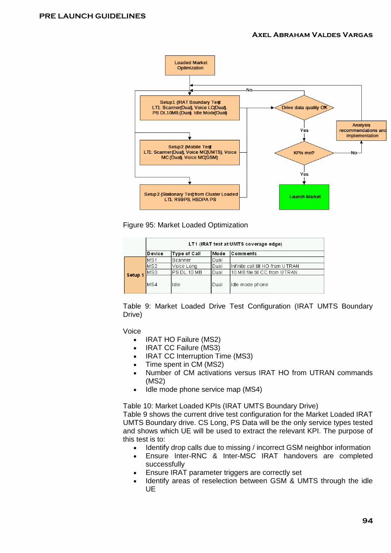
PRE LAUNCH GUIDELINES
Axel Abraham Valdes Vargas
94
Figure 95: Market Loaded Optimization
Table 9: Market Loaded Drive Test Configuration (IRAT UMTS Boundary Drive) Voice
• IRAT HO Failure (MS2) • IRAT CC Failure (MS3) • IRAT CC Interruption Time (MS3) • Time spent in CM (MS2) • Number of CM activations versus IRAT HO from UTRAN commands
(MS2) • Idle mode phone service map (MS4)
Table 10: Market Loaded KPIs (IRAT UMTS Boundary Drive) Table 9 shows the current drive test configuration for the Market Loaded IRAT UMTS Boundary drive. CS Long, PS Data will be the only service types tested and shows which UE will be used to extract the relevant KPI. The purpose of this test is to:
• Identify drop calls due to missing / incorrect GSM neighbor information • Ensure Inter-RNC & Inter-MSC IRAT handovers are completed
successfully • Ensure IRAT parameter triggers are correctly set • Identify areas of reselection between GSM & UMTS through the idle
UE

PRE LAUNCH GUIDELINES
Axel Abraham Valdes Vargas
95
Table 11: Market Loaded Drive Test Configuration (User Experience Mobile Test)
Table 12: Market Loaded KPIs (User Experience Mobile Test) Table 11 shows the current drive test configuration for the Market Loaded User Experience Mobile Test. CS Long, GSM Long & Dual mode UE will be tested and Table 12 shows which UE will be used to extract the relevant KPI. The purpose of this test is to:
• Identify IRAT is working properly within the UMTS coverage areas • Identify drop calls due to missing / incorrect GSM neighbor information • Ensure IRAT parameter triggers are correctly set • Provide benchmarking results between UMTS & GSM
Whilst the drive test configurations & KPIs have been shown above, this document will not provide details regarding how to perform drive tests. 5.3.IRAT Handover Failure Analysis This section provides guidelines on how to trouble-shoot IRAT handover failures that was reported in the KPI post processing report. It is not the intention to provide an explanation on what IRAT Handover is or how it works, the assumption is that the reader has the required background knowledge. 5.3.1.Identifying IRAT Handover Failures: The IRAT handover can fail at various different phases during the handover process. Depending on how the KPI is specified, not all of these failures are counted in the KPI or recorded in the drive test tools as failed IRAT Handover attempts. Therefore the first step is to clarify the definition of an IRAT HO failure. The following diagram shows the high level handover process and how IRAT Handover failures are detected.

PRE LAUNCH GUIDELINES
Axel Abraham Valdes Vargas
96
Figure 96: IRAT Handover Process Summary From the above diagram the KPI formula for calculating the Handover failure rate can be easily interpreted:
Equation 4: CSV Handover Failure Rate 5.3.2.IRAT Handover Failure Trouble Shooting Process The 1st step is to determine if IRAT handover is failing for all the cells on the RNC or is the problem related to a cell specific issue. Before cell level IRAT handover failure analysis is attempted it is imperative to verify that IRAT Handover is configured in both the 2G and 3G networks end to end. Note IRAT handover tests are not performed during Site Acceptance testing. Once IRAT handover is confirmed working for at least one cell on the RNC it will prove that the core networks are configured correctly and one can proceed with cell level faultfinding.

PRE LAUNCH GUIDELINES
Axel Abraham Valdes Vargas
97
The 2nd step is to determine if IRAT HO attempts was suppose to happen at that location. IRAT HO in the core UMTS coverage area should be minimal. The purpose of this part of the process is to establish if the IRAT attempt was triggered unnecessarily due to a problem on the UMTS network. The three triggers used to start CM are:
• Bad Ec/No • Low RSCP • High UE Tx Power
All of these can be triggered due to problems on the UMTS network which would not cause IRAT Handover under normal conditions. The aim is to eliminate these “false” IRAT attempts by rectifying the UMTS network rather than to fault finding why the IRAT Handover attempt failed. If it was determined that the IRAT Handover attempt occurred due to a legitimate reason then the detailed faultfinding process as discussed in the remainder of this document must be followed.
Figure 97: IRAT Handover Analysis 5.3.3. Global IRAT handover failures:

PRE LAUNCH GUIDELINES
Axel Abraham Valdes Vargas
98
The 1st step in IRAT analysis is to determine if IRAT Handover is working at all. For IRAT handover to be possible all the sub-systems in chain have to be correctly provisioned: Starting from the UE to NodeB to RNC to 3GMSC to 2G-MSC to BSC to BTS. 5.3.3.1.IRAT prerequisites: The UTRAN network needs to support the following:
• UE UTRAN downlink measurement activation • Associated RANAP protocol and procedures on Iu • Associated RRC protocol and procedures • Broadcast of the following on the BCCH:
o The inter-RAT (GSM) neighbor cell information o Measurement capability IE and extension o UE capability IE and extension, UE Classmark o System information, ciphering information etc;
The core network needs to support the following:
• Location registration update from 3G to/from 2G cell, for PS or CS • Ability to convert the 3G ciphering key to/from the 2G ciphering key • Associated RANAP protocol and procedures on Iu • Ability to convert 3G QoS attributes to/from 2G attributes • BSSMAP to RANAP message inter-working to support message
conversion and deriving GSM channel type from the WCDMA RAB attributes, and vice versa
By confirming the IRAT functionality on one cell it will at least verify that the core networks are correctly configured. The aim of this document is not to explain the details on how to configure the core networks to allow for IRAT HO but to focus on faultfinding individual IRAT HO failures. 5.3.4. Cell Specific IRAT failures This section focuses on how to trouble shoot IRAT handover failures on a cell or per call level and it assumes that IRAT functionality has been proven on the cell at some stage. (At least to the point that the UE will be send the command HandoverfromUTRAN after it reports event 2d and 3a). As described above the first step is to establish whether the IRAT attempt was supposed to occur at this location or not. This analysis will require looking at the drive survey file in detail to establish the network conditions at the point of failure. The process for this analysis is as follow:
• Open the logfile in Actix • Display the Ec/No of the strongest cell in the Active set on the map • Display the RSCP of the strongest cell in the Active set on the map • Display the UE Tx power on the map • Display the Events on the map. • Display both the GSM and UMTS scanner to see if strongest cell was
in the active set and the best GSM cell was used as the target handover cell. (Basically check for missing neighbors)

PRE LAUNCH GUIDELINES
Axel Abraham Valdes Vargas
99
• Locate the IRAT Handover failures on the map and note the Receiver signal strength and quality as well as the UE TX power at this location
Figure 98: IRAT Handover Validity From the above diagram, a decision must be made whether the IRAT attempt was suppose to happen at this location. The guideline for making this decision is based on the following criteria:
• Any IRAT attempt that occurred while leaving the UMTS coverage area (edge of UMTS coverage) is most likely a legitimate attempt
• If the IRAT attempt happens inside the core UMTS polygon it will depend on the trigger for the CM if it was supposed to happen
• Assuming the default IRAT handover parameter values as per baseline, IRAT triggers due to RSCP means that there is a lack of coverage and therefore the IRAT attempt can be valid (assuming there is nothing that can be done to the antenna system to improve the coverage at this location). These attempts need to be validated by the fact that there is a UMTS coverage hole inside the polygon.
• If the IRAT trigger was due to Ec/No it can point to quality issues cause by pilot pollution, interference, missing neighbor, over-shooting cells etc. The route cause of the bad quality will have to be identified and corrected.
• If the IRAT was triggered due to Maximum UE Tx Power, it can point to uplink interference. This can be verified by looking at the Uplink RSSI counters. These IRAT attempts are also not considered attempts that are supposed to be happening.
The following section provides details on how to trouble shoot the valid IRAT handover failures: It is helpful to establish during which stage of the IRAT HO the failure occurred as this assists in the trouble shooting process. IRAT failures can be sub divided into 3 categories depending on which stage the handover failure occurred:
• Preparation phase failure

PRE LAUNCH GUIDELINES
Axel Abraham Valdes Vargas
100
• Execution phase failures • Confirmation phase failures.
Figure 99 shows the three different IRAT HO stages.
Figure 99: IRAT Handover Stages 5.3.4.1 Preparation Phase Failure Note as shown in Figure 99, failures in compressed mode activation or even dropped calls due to CM are not included in the IRAT HO KPI consideration and from Figure 99 above it can be seen that this is also not included in the preparation phase either. The main constraints for allowing the UE to enter into CM is the additional resources required for CM from the Radio Link point of view, higher Tx power and more Downlink Codes due to the higher SF requirement. This is mainly an issue that can impact the IRAT Handover in a loaded network. The maximum number of UEs that can be in CM per cell is also fixed as per the parameter compModeAdm which is currently set to 15. The implication is that if 15 UEs on the cell are already in CM, it can result in then next IRAT HO request being denied by the admission control. Note from experience hanging compressed mode resources is a common problem and can result in dropped calls due to IRAT Handover not possible because CM was denied. Therefore it is recommended to look at the number of UE in compressed mode to verify that this limit had not been exceeded. (This is obviously not an issue in the pre-launch optimization phase) The main activities performed by the RNC during the preparation phase is to negotiate resources with the 2G network so that the necessary resources are allocated for the IRAT HO to proceed. The preparation phase starts when the UE sends the measurement report “Event 3a” containing the information of the target GSM cells. The preparation phase stops when the RNC sends out the Handover from UTRAN command. Preparation phase failures are normally not included in the KPI for calculating IRAT handover failures. The common counter KPI formula for calculating IRAT HO is given by the following equation:

PRE LAUNCH GUIDELINES
Axel Abraham Valdes Vargas
101
Figure 100: IRAT HO KPI This formula will not show preparation failures as it only starts pegging an IRAT Attempt when the Handover from UTRAN command is sent to the UE. Any failures prior to this are classified as Preparation phase failures. Most of the preparation phase failures can be identified by the counter pmNoFailOutIratHoSpeachGsmFail. Note during drive survey analysis these failures are not pegged as IRAT handover failures for the HandoverfromUTRAN command has not been sent to the UE. The reason why the HandoverfromUTRAN message was not received by the UE can be either it was not sent by RNC or it was sent and never received by UE due to loss of radio signal. Reasons why the RNC will not sent the HandoverfromUTRAN command can be because:
• RNC could not negotiate the resources with the BSS • RNC never received the event 3a from the UE (note for the counter
analysis this will not be the case for the KPI only starts pegging once the event 3a measurement report is received by RNC)
Common causes for failures during this stage:
• Incorrect external GSM cell definitions on the UMTS OSS ( Incorrect LAC, BSIC, BCCH)
• Congestion on the target GSM cell. • Incorrect foreign LAC information in the MSC. • Problems in the GSM core network. • Lac of resources in the 3G network.
Trouble-Shooting Preparation Phase Failures: Incorrect external GSM cell definitions: It is imperative that the GSM cell definitions are up to date in the RNC, this will require a regular audit to ensure that the databases are in synch. Main problem is that when changes are made on the 2G network (for instance a Frequency retune) the UMTS network will have to be updated manually. (Assuming 3G and 2G networks are using different vendor’s equipment) These failures are mostly identified by a sudden increase in preparation phase failures (from stats) which can indicate possible changes in the 2G network. Solution to this problem is to compare a dump from the GSM network with a dump from the 3G network and correct any discrepancies. (More detail process is currently in production) Problems with GSM cells:
PRE LAUNCH GUIDELINES
Axel Abraham Valdes Vargas
102
A sudden increase in preparation phase failures for an individual handover relation can point to problems with the GSM cell. Fault finding these problems will require access to the GSM OSS to verify if the GSM cell had any alarms (hardware or software issues) during the same time. It is helpful to look at the 2G to 2G handover stats for the target GSM cell to verify if the cell had any problems. Confirm that there is no congestion on the GSM cell that can result in blocked handover attempt from UMTS. Incorrect foreign LAC information in the MSC: This is a data fill issue which is often overlooked when re-homes across a BSC is done or if new BSC (LAC) is introduced. The core network team are responsible for maintaining the LAC tables on the MSCs. 5.3.4.2. Execution phase failures. These IRAT HO failures are similar to GSM handover failures where the handover is attempted but cannot be completed and the UE reverts to the original cell. These are the IRAT HO failures that will be recorded by the drive survey post processing KPI module. This is important to note as it is just a handover failure and not a drop call. (Needless to say the handover failure can result in a drop call at a later stage). In the IRAT handover call-flow diagram above, the execution phase starts when the command “Handover from UTRAN” is send from the RNC to the UE. Failures during the execution phase are mostly identified by the counter: pmNoHoSpeechRetOldChPhyChFail. Common reasons for failures during the Execution phase:
• RF related failures: o Rapid Field drop, o Poor Quality on UMTS o Poor Quality on GSM o Rapidly changing radio environment o Deep fades o No Dominant server o Low best serving CPICH RSPCH/Ptotal etc. Refer to 4.4.4 on
coverage analysis to trouble shoot these problems • RF link unbalance, if downlink coverage is larger than uplink coverage
area the CM will start too late and UE will not have enough power to get back to NodeB and call will drop. (Refer to 4.4.4)
• BSIC or BCCH confusion. Refer to GSM engineer for correction. • Missing IRAT handover definitions. Verify from the GSM scanner that
the best GSM cell was selected for the handover attempt. In the uplink measurement reports (from layer 3 messages) verify that the correct BSIC was verified
• Incorrect handover parameters. It is very important to confirm that base line parameters were applied. It is not the intention of this document to provide an explanation as to what the impact will be if IRAT Handover parameters are changed. It is essential for the engineer to realize that changing any of the IRAT parameters should only be done by someone that has the relevant experience to understand the impact of making those changes. Changing one parameter in isolation will most likely cause problems elsewhere that’s the reason why we refer to an IRAT parameter set.

PRE LAUNCH GUIDELINES
Axel Abraham Valdes Vargas
103
• Problems on the target GSM cell. This can be hardware, interference etc verify the GSM handover performance from XPM.
• Core network issues. To trouble shoot core network issues contact UTRAN support.
• Hardware problems on the serving UMTS cell. (Check alarm history for any problems while the drive test was done)
• Bad quality on the serving UMTS cell (Mostly caused due to pilot pollution, lack of dominance, lack UMTS coverage, incorrect power measurements due to incorrect TMA parameter settings. For more information on trouble shooting these problems refer to 4.4.4)
Trouble shooting execution phase failures are done by analyzing the drive test files. It is also helpful to have the UE trace file available to confirm the messages that was received in the RNC. For more detailed trouble shooting Geoprobe traces can also be helpful. This section will provide a brief overview of how to identify the causes for the IRAT Failure when looking at a drive survey log file in Actix analyzer. Procedure for analyzing the IRAT handover failures in Actix:
• Load the Logfiles in Actix • Ensure that an updated cell ref file is loaded containing the UMTS and
GSM cells as per the configuration for the day the drive was done. (Will have a process to produce daily cell ref files)
• Display the Ec/No and RSCP for the strongest cell in the active set on the map
• Add the events to the map. (IRAT handover failures) • Note the signal levels on UMTS before the failure • Find the IRAT Handover reason(cause) • Look at the layer 3 messaging for the IRAT neighbor list that was send
to the UE, first step is to validate that the correct list was send to the UE, was the obvious required neighbors in the list. If not this can be the reason why the Handover failed
• Look at the stats and alarm list for the targeted GSM cell (this will have to be done in XMP or similar system)
• Look at the signal strength for the measured neighboring cells (details in the measurement reports send by the UE)
• Verify that there were no BCCH/ BSIC confusion possibilities. (MapInfo analysis is recommended)
In the layer 3 messaging look for any missing messages that can provide a clue as to why the IRAT handover failed. The UE must follow the sequence as below.
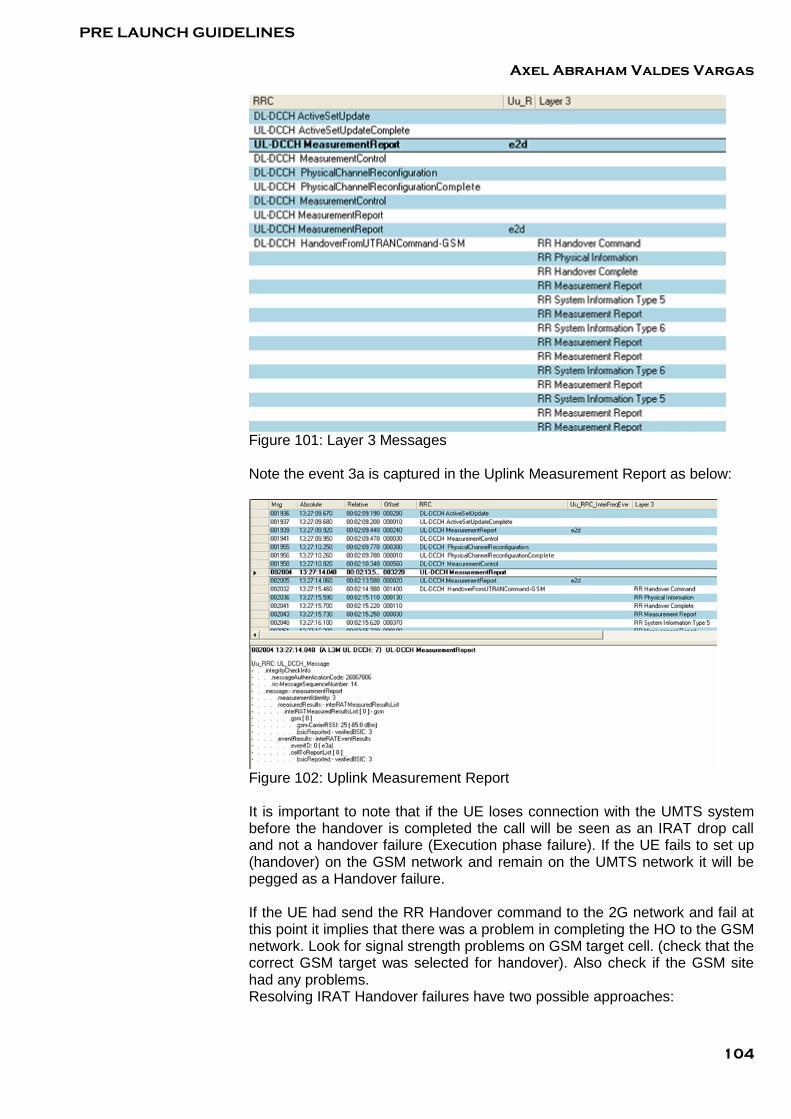
PRE LAUNCH GUIDELINES
Axel Abraham Valdes Vargas
104
Figure 101: Layer 3 Messages Note the event 3a is captured in the Uplink Measurement Report as below:
Figure 102: Uplink Measurement Report It is important to note that if the UE loses connection with the UMTS system before the handover is completed the call will be seen as an IRAT drop call and not a handover failure (Execution phase failure). If the UE fails to set up (handover) on the GSM network and remain on the UMTS network it will be pegged as a Handover failure. If the UE had send the RR Handover command to the 2G network and fail at this point it implies that there was a problem in completing the HO to the GSM network. Look for signal strength problems on GSM target cell. (check that the correct GSM target was selected for handover). Also check if the GSM site had any problems. Resolving IRAT Handover failures have two possible approaches:
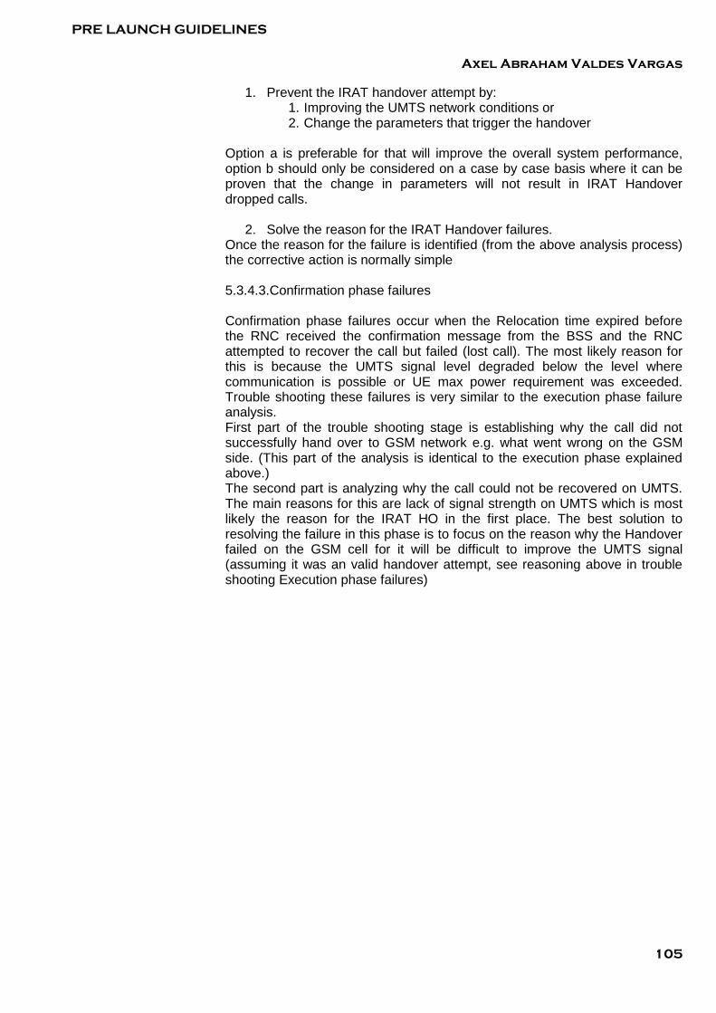
PRE LAUNCH GUIDELINES
Axel Abraham Valdes Vargas
105
1. Prevent the IRAT handover attempt by: 1. Improving the UMTS network conditions or 2. Change the parameters that trigger the handover
Option a is preferable for that will improve the overall system performance, option b should only be considered on a case by case basis where it can be proven that the change in parameters will not result in IRAT Handover dropped calls.
2. Solve the reason for the IRAT Handover failures. Once the reason for the failure is identified (from the above analysis process) the corrective action is normally simple 5.3.4.3.Confirmation phase failures Confirmation phase failures occur when the Relocation time expired before the RNC received the confirmation message from the BSS and the RNC attempted to recover the call but failed (lost call). The most likely reason for this is because the UMTS signal level degraded below the level where communication is possible or UE max power requirement was exceeded. Trouble shooting these failures is very similar to the execution phase failure analysis. First part of the trouble shooting stage is establishing why the call did not successfully hand over to GSM network e.g. what went wrong on the GSM side. (This part of the analysis is identical to the execution phase explained above.) The second part is analyzing why the call could not be recovered on UMTS. The main reasons for this are lack of signal strength on UMTS which is most likely the reason for the IRAT HO in the first place. The best solution to resolving the failure in this phase is to focus on the reason why the Handover failed on the GSM cell for it will be difficult to improve the UMTS signal (assuming it was an valid handover attempt, see reasoning above in trouble shooting Execution phase failures)