practical foundations for programming languagesgiangi/corsi/pr2/harperbook.pdf · practical...
TRANSCRIPT
Practical Foundations for ProgrammingLanguages
Robert HarperCarnegie Mellon University
Spring, 2011
[Version 1.2 of 03.02.11.]
Copyright c! 2010 by Robert Harper.
All Rights Reserved.
The electronic version of this work is licensed under the Cre-ative Commons Attribution-Noncommercial-No Derivative Works3.0 United States License. To view a copy of this license, visit
http://creativecommons.org/licenses/by-nc-nd/3.0/us/
or send a letter to Creative Commons, 171 Second Street, Suite300, San Francisco, California, 94105, USA.
Preface
This is a working draft of a book on the foundations of programming lan-guages. The central organizing principle of the book is that programminglanguage features may be seen as manifestations of an underlying typestructure that governs its syntax and semantics. The emphasis, therefore,is on the concept of type, which codifies and organizes the computationaluniverse in much the same way that the concept of set may be seen as anorganizing principle for the mathematical universe. The purpose of thisbook is to explain this remark.
This is very much a work in progress, with major revisions made nearlyevery day. This means that there may be internal inconsistencies as revi-sions to one part of the book invalidate material at another part. Pleasebear this in mind!
Corrections, comments, and suggestions are most welcome, and shouldbe sent to the author at [email protected]. I am grateful to the following peo-ple for their comments, corrections, and suggestions to various versionsof this book: Arbob Ahmad, Andrew Appel, Zena Ariola, Guy E. Blel-loch, William Byrd, Luca Cardelli, Iliano Cervesato, Manuel Chakravarti,Richard C. Cobbe, Karl Crary, Daniel Dantas, Anupam Datta, Jake Don-ham, Derek Dreyer, Matthias Felleisen, Frank Pfenning, Dan Friedman,Maia Ginsburg, Kevin Hely, Cao Jing, Gabriele Keller, Danielle Kramer,Akiva Leffert, Ruy Ley-Wild, Dan Licata, Karen Liu, Dave MacQueen, ChrisMartens, Greg Morrisett, Tom Murphy, Aleksandar Nanevski, Georg Neis,David Neville, Doug Perkins, Frank Pfenning, Benjamin C. Pierce, AndrewM. Pitts, Gordon D. Plotkin, David Renshaw, John C. Reynolds, Carter T.Schonwald, Dale Schumacher, Dana Scott, Zhong Shao, Robert Simmons,Pawel Sobocinski, Daniel Spoonhower, Paulo Tanimoto, Michael Tschantz,Kami Vaniea, Carsten Varming, David Walker, Dan Wang, Jack Wileden,Todd Wilson, Roger Wolff, Luke Zarko, Yu Zhang.
This material is based upon work supported by the National ScienceFoundation under Grant Nos. 0702381 and 0716469. Any opinions, find-
ings, and conclusions or recommendations expressed in this material arethose of the author(s) and do not necessarily reflect the views of the Na-tional Science Foundation.
The support of the Max Planck Institute for Software Systems in Saarbrucken,Germany is gratefully acknowledged.
Contents
Preface iii
I Judgements and Rules 1
1 Inductive Definitions 31.1 Judgements . . . . . . . . . . . . . . . . . . . . . . . . . . . . 31.2 Inference Rules . . . . . . . . . . . . . . . . . . . . . . . . . . 41.3 Derivations . . . . . . . . . . . . . . . . . . . . . . . . . . . . . 51.4 Rule Induction . . . . . . . . . . . . . . . . . . . . . . . . . . . 71.5 Iterated and Simultaneous Inductive Definitions . . . . . . . 91.6 Defining Functions by Rules . . . . . . . . . . . . . . . . . . . 111.7 Modes . . . . . . . . . . . . . . . . . . . . . . . . . . . . . . . 121.8 Exercises . . . . . . . . . . . . . . . . . . . . . . . . . . . . . . 13
2 Hypothetical Judgements 152.1 Derivability . . . . . . . . . . . . . . . . . . . . . . . . . . . . 152.2 Admissibility . . . . . . . . . . . . . . . . . . . . . . . . . . . 172.3 Hypothetical Inductive Definitions . . . . . . . . . . . . . . . 192.4 Exercises . . . . . . . . . . . . . . . . . . . . . . . . . . . . . . 21
3 Syntax Trees 233.1 Abstract Syntax Trees . . . . . . . . . . . . . . . . . . . . . . . 233.2 Abstract Binding Trees . . . . . . . . . . . . . . . . . . . . . . 253.3 Parameterization . . . . . . . . . . . . . . . . . . . . . . . . . 303.4 Exercises . . . . . . . . . . . . . . . . . . . . . . . . . . . . . . 32
4 Generic Judgements 334.1 Rule Schemes . . . . . . . . . . . . . . . . . . . . . . . . . . . 334.2 Generic Derivability . . . . . . . . . . . . . . . . . . . . . . . 34

vi CONTENTS
4.3 Generic Inductive Definitions . . . . . . . . . . . . . . . . . . 354.4 Parametric Derivability . . . . . . . . . . . . . . . . . . . . . . 364.5 Exercises . . . . . . . . . . . . . . . . . . . . . . . . . . . . . . 37
II Levels of Syntax 39
5 Concrete Syntax 415.1 Strings Over An Alphabet . . . . . . . . . . . . . . . . . . . . 415.2 Lexical Structure . . . . . . . . . . . . . . . . . . . . . . . . . 425.3 Context-Free Grammars . . . . . . . . . . . . . . . . . . . . . 465.4 Grammatical Structure . . . . . . . . . . . . . . . . . . . . . . 475.5 Ambiguity . . . . . . . . . . . . . . . . . . . . . . . . . . . . . 485.6 Exercises . . . . . . . . . . . . . . . . . . . . . . . . . . . . . . 50
6 Abstract Syntax 516.1 Hierarchical and Binding Structure . . . . . . . . . . . . . . . 516.2 Parsing Into Abstract Syntax Trees . . . . . . . . . . . . . . . 536.3 Parsing Into Abstract Binding Trees . . . . . . . . . . . . . . . 556.4 Exercises . . . . . . . . . . . . . . . . . . . . . . . . . . . . . . 57
III Statics and Dynamics 59
7 Statics 617.1 Syntax . . . . . . . . . . . . . . . . . . . . . . . . . . . . . . . 617.2 Type System . . . . . . . . . . . . . . . . . . . . . . . . . . . . 627.3 Structural Properties . . . . . . . . . . . . . . . . . . . . . . . 647.4 Exercises . . . . . . . . . . . . . . . . . . . . . . . . . . . . . . 66
8 Dynamics 678.1 Transition Systems . . . . . . . . . . . . . . . . . . . . . . . . 678.2 Structural Dynamics . . . . . . . . . . . . . . . . . . . . . . . 688.3 Contextual Dynamics . . . . . . . . . . . . . . . . . . . . . . . 718.4 Equational Dynamics . . . . . . . . . . . . . . . . . . . . . . . 738.5 Exercises . . . . . . . . . . . . . . . . . . . . . . . . . . . . . . 76
9 Type Safety 779.1 Preservation . . . . . . . . . . . . . . . . . . . . . . . . . . . . 789.2 Progress . . . . . . . . . . . . . . . . . . . . . . . . . . . . . . 789.3 Run-Time Errors . . . . . . . . . . . . . . . . . . . . . . . . . . 80
VERSION 1.2 DRAFT REVISED 03.02.11
CONTENTS vii
9.4 Exercises . . . . . . . . . . . . . . . . . . . . . . . . . . . . . . 81
10 Evaluation Dynamics 8310.1 Evaluation Dynamics . . . . . . . . . . . . . . . . . . . . . . . 8310.2 Relating Structural and Evaluation Dynamics . . . . . . . . . 8410.3 Type Safety, Revisited . . . . . . . . . . . . . . . . . . . . . . . 8510.4 Cost Dynamics . . . . . . . . . . . . . . . . . . . . . . . . . . 8710.5 Exercises . . . . . . . . . . . . . . . . . . . . . . . . . . . . . . 88
IV Function Types 89
11 Function Definitions and Values 9111.1 First-Order Functions . . . . . . . . . . . . . . . . . . . . . . . 9211.2 Higher-Order Functions . . . . . . . . . . . . . . . . . . . . . 9311.3 Evaluation Dynamics and Definitional Equivalence . . . . . 9511.4 Dynamic Scope . . . . . . . . . . . . . . . . . . . . . . . . . . 9711.5 Exercises . . . . . . . . . . . . . . . . . . . . . . . . . . . . . . 98
12 Godel’s System T 9912.1 Statics . . . . . . . . . . . . . . . . . . . . . . . . . . . . . . . . 10012.2 Dynamics . . . . . . . . . . . . . . . . . . . . . . . . . . . . . 10112.3 Definability . . . . . . . . . . . . . . . . . . . . . . . . . . . . 10212.4 Non-Definability . . . . . . . . . . . . . . . . . . . . . . . . . 10412.5 Exercises . . . . . . . . . . . . . . . . . . . . . . . . . . . . . . 106
13 Plotkin’s PCF 10713.1 Statics . . . . . . . . . . . . . . . . . . . . . . . . . . . . . . . . 10913.2 Dynamics . . . . . . . . . . . . . . . . . . . . . . . . . . . . . 11013.3 Definability . . . . . . . . . . . . . . . . . . . . . . . . . . . . 11213.4 Co-Natural Numbers . . . . . . . . . . . . . . . . . . . . . . . 11413.5 Exercises . . . . . . . . . . . . . . . . . . . . . . . . . . . . . . 114
V Finite Data Types 115
14 Product Types 11714.1 Nullary and Binary Products . . . . . . . . . . . . . . . . . . 11814.2 Finite Products . . . . . . . . . . . . . . . . . . . . . . . . . . 11914.3 Primitive and Mutual Recursion . . . . . . . . . . . . . . . . 12114.4 Exercises . . . . . . . . . . . . . . . . . . . . . . . . . . . . . . 122
REVISED 03.02.11 DRAFT VERSION 1.2
viii CONTENTS
15 Sum Types 12315.1 Binary and Nullary Sums . . . . . . . . . . . . . . . . . . . . 12315.2 Finite Sums . . . . . . . . . . . . . . . . . . . . . . . . . . . . 12515.3 Applications of Sum Types . . . . . . . . . . . . . . . . . . . . 126
15.3.1 Void and Unit . . . . . . . . . . . . . . . . . . . . . . . 12615.3.2 Booleans . . . . . . . . . . . . . . . . . . . . . . . . . . 12715.3.3 Enumerations . . . . . . . . . . . . . . . . . . . . . . . 12715.3.4 Options . . . . . . . . . . . . . . . . . . . . . . . . . . 128
15.4 Exercises . . . . . . . . . . . . . . . . . . . . . . . . . . . . . . 129
16 Pattern Matching 13116.1 A Pattern Language . . . . . . . . . . . . . . . . . . . . . . . . 13216.2 Statics . . . . . . . . . . . . . . . . . . . . . . . . . . . . . . . . 13216.3 Dynamics . . . . . . . . . . . . . . . . . . . . . . . . . . . . . 13416.4 Exhaustiveness and Redundancy . . . . . . . . . . . . . . . . 136
16.4.1 Match Constraints . . . . . . . . . . . . . . . . . . . . 13616.4.2 Enforcing Exhaustiveness and Redundancy . . . . . . 13816.4.3 Checking Exhaustiveness and Redundancy . . . . . . 139
16.5 Exercises . . . . . . . . . . . . . . . . . . . . . . . . . . . . . . 140
17 Generic Programming 14117.1 Introduction . . . . . . . . . . . . . . . . . . . . . . . . . . . . 14117.2 Type Operators . . . . . . . . . . . . . . . . . . . . . . . . . . 14217.3 Generic Extension . . . . . . . . . . . . . . . . . . . . . . . . . 14217.4 Exercises . . . . . . . . . . . . . . . . . . . . . . . . . . . . . . 145
VI Infinite Data Types 147
18 Inductive and Co-Inductive Types 14918.1 Motivating Examples . . . . . . . . . . . . . . . . . . . . . . . 14918.2 Statics . . . . . . . . . . . . . . . . . . . . . . . . . . . . . . . . 153
18.2.1 Types . . . . . . . . . . . . . . . . . . . . . . . . . . . . 15318.2.2 Expressions . . . . . . . . . . . . . . . . . . . . . . . . 154
18.3 Dynamics . . . . . . . . . . . . . . . . . . . . . . . . . . . . . 15418.4 Exercises . . . . . . . . . . . . . . . . . . . . . . . . . . . . . . 155
19 Recursive Types 15719.1 Solving Type Isomorphisms . . . . . . . . . . . . . . . . . . . 15819.2 Recursive Data Structures . . . . . . . . . . . . . . . . . . . . 159
VERSION 1.2 DRAFT REVISED 03.02.11
CONTENTS ix
19.3 Self-Reference . . . . . . . . . . . . . . . . . . . . . . . . . . . 16119.4 Exercises . . . . . . . . . . . . . . . . . . . . . . . . . . . . . . 163
VII Dynamic Types 165
20 The Untyped !-Calculus 16720.1 The !-Calculus . . . . . . . . . . . . . . . . . . . . . . . . . . 16720.2 Definability . . . . . . . . . . . . . . . . . . . . . . . . . . . . 16920.3 Scott’s Theorem . . . . . . . . . . . . . . . . . . . . . . . . . . 17120.4 Untyped Means Uni-Typed . . . . . . . . . . . . . . . . . . . 17320.5 Exercises . . . . . . . . . . . . . . . . . . . . . . . . . . . . . . 175
21 Dynamic Typing 17721.1 Dynamically Typed PCF . . . . . . . . . . . . . . . . . . . . . 17721.2 Variations and Extensions . . . . . . . . . . . . . . . . . . . . 18021.3 Critique of Dynamic Typing . . . . . . . . . . . . . . . . . . . 18321.4 Exercises . . . . . . . . . . . . . . . . . . . . . . . . . . . . . . 184
22 Hybrid Typing 18522.1 A Hybrid Language . . . . . . . . . . . . . . . . . . . . . . . . 18522.2 Optimization of Dynamic Typing . . . . . . . . . . . . . . . . 18722.3 Static “Versus” Dynamic Typing . . . . . . . . . . . . . . . . 18922.4 Reduction to Recursive Types . . . . . . . . . . . . . . . . . . 190
VIII Variable Types 191
23 Girard’s System F 19323.1 System F . . . . . . . . . . . . . . . . . . . . . . . . . . . . . . 19423.2 Polymorphic Definability . . . . . . . . . . . . . . . . . . . . 197
23.2.1 Products and Sums . . . . . . . . . . . . . . . . . . . . 19723.2.2 Natural Numbers . . . . . . . . . . . . . . . . . . . . . 198
23.3 Parametricity Overview . . . . . . . . . . . . . . . . . . . . . 19923.4 Restricted Forms of Polymorphism . . . . . . . . . . . . . . . 201
23.4.1 Predicative Fragment . . . . . . . . . . . . . . . . . . . 20123.4.2 Prenex Fragment . . . . . . . . . . . . . . . . . . . . . 20223.4.3 Rank-Restricted Fragments . . . . . . . . . . . . . . . 204
23.5 Exercises . . . . . . . . . . . . . . . . . . . . . . . . . . . . . . 205
REVISED 03.02.11 DRAFT VERSION 1.2
x CONTENTS
24 Abstract Types 20724.1 Existential Types . . . . . . . . . . . . . . . . . . . . . . . . . 208
24.1.1 Statics . . . . . . . . . . . . . . . . . . . . . . . . . . . 20824.1.2 Dynamics . . . . . . . . . . . . . . . . . . . . . . . . . 20924.1.3 Safety . . . . . . . . . . . . . . . . . . . . . . . . . . . . 210
24.2 Data Abstraction Via Existentials . . . . . . . . . . . . . . . . 21024.3 Definability of Existentials . . . . . . . . . . . . . . . . . . . . 21224.4 Representation Independence . . . . . . . . . . . . . . . . . . 21324.5 Exercises . . . . . . . . . . . . . . . . . . . . . . . . . . . . . . 215
25 Constructors and Kinds 21725.1 Statics . . . . . . . . . . . . . . . . . . . . . . . . . . . . . . . . 21825.2 Adding Constructors and Kinds . . . . . . . . . . . . . . . . 22025.3 Substitution . . . . . . . . . . . . . . . . . . . . . . . . . . . . 22225.4 Exercises . . . . . . . . . . . . . . . . . . . . . . . . . . . . . . 225
26 Indexed Families of Types 22726.1 Type Families . . . . . . . . . . . . . . . . . . . . . . . . . . . 22726.2 Exercises . . . . . . . . . . . . . . . . . . . . . . . . . . . . . . 227
IX Subtyping 229
27 Subtyping 23127.1 Subsumption . . . . . . . . . . . . . . . . . . . . . . . . . . . . 23227.2 Varieties of Subtyping . . . . . . . . . . . . . . . . . . . . . . 232
27.2.1 Numeric Types . . . . . . . . . . . . . . . . . . . . . . 23227.2.2 Product Types . . . . . . . . . . . . . . . . . . . . . . . 23327.2.3 Sum Types . . . . . . . . . . . . . . . . . . . . . . . . . 235
27.3 Variance . . . . . . . . . . . . . . . . . . . . . . . . . . . . . . 23627.3.1 Product Types . . . . . . . . . . . . . . . . . . . . . . . 23627.3.2 Sum Types . . . . . . . . . . . . . . . . . . . . . . . . . 23627.3.3 Function Types . . . . . . . . . . . . . . . . . . . . . . 23727.3.4 Recursive Types . . . . . . . . . . . . . . . . . . . . . . 238
27.4 Safety for Subtyping . . . . . . . . . . . . . . . . . . . . . . . 24027.5 Exercises . . . . . . . . . . . . . . . . . . . . . . . . . . . . . . 242
28 Singleton and Dependent Kinds 24328.1 Informal Overview . . . . . . . . . . . . . . . . . . . . . . . . 244
VERSION 1.2 DRAFT REVISED 03.02.11
CONTENTS xi
X Classes and Methods 247
29 Dynamic Dispatch 24929.1 The Dispatch Matrix . . . . . . . . . . . . . . . . . . . . . . . 25129.2 Method-Based Organization . . . . . . . . . . . . . . . . . . . 25329.3 Class-Based Organization . . . . . . . . . . . . . . . . . . . . 25429.4 Self-Reference . . . . . . . . . . . . . . . . . . . . . . . . . . . 25529.5 Exercises . . . . . . . . . . . . . . . . . . . . . . . . . . . . . . 257
30 Inheritance 25930.1 Subclassing . . . . . . . . . . . . . . . . . . . . . . . . . . . . . 26030.2 Exercises . . . . . . . . . . . . . . . . . . . . . . . . . . . . . . 263
XI Control Effects 265
31 Control Stacks 26731.1 Machine Definition . . . . . . . . . . . . . . . . . . . . . . . . 26731.2 Safety . . . . . . . . . . . . . . . . . . . . . . . . . . . . . . . . 26931.3 Correctness of the Control Machine . . . . . . . . . . . . . . . 270
31.3.1 Completeness . . . . . . . . . . . . . . . . . . . . . . . 27231.3.2 Soundness . . . . . . . . . . . . . . . . . . . . . . . . . 272
31.4 Exercises . . . . . . . . . . . . . . . . . . . . . . . . . . . . . . 273
32 Exceptions 27532.1 Failures . . . . . . . . . . . . . . . . . . . . . . . . . . . . . . . 27532.2 Exceptions . . . . . . . . . . . . . . . . . . . . . . . . . . . . . 27732.3 Exception Type . . . . . . . . . . . . . . . . . . . . . . . . . . 27832.4 Encapsulation . . . . . . . . . . . . . . . . . . . . . . . . . . . 28032.5 Exercises . . . . . . . . . . . . . . . . . . . . . . . . . . . . . . 282
33 Continuations 28333.1 Informal Overview . . . . . . . . . . . . . . . . . . . . . . . . 28333.2 Semantics of Continuations . . . . . . . . . . . . . . . . . . . 28533.3 Coroutines . . . . . . . . . . . . . . . . . . . . . . . . . . . . . 28733.4 Exercises . . . . . . . . . . . . . . . . . . . . . . . . . . . . . . 291
XII Types and Propositions 293
34 Constructive Logic 295
REVISED 03.02.11 DRAFT VERSION 1.2
xii CONTENTS
34.1 Constructive Semantics . . . . . . . . . . . . . . . . . . . . . . 29634.2 Constructive Logic . . . . . . . . . . . . . . . . . . . . . . . . 297
34.2.1 Rules of Provability . . . . . . . . . . . . . . . . . . . . 29834.2.2 Rules of Proof . . . . . . . . . . . . . . . . . . . . . . . 300
34.3 Propositions as Types . . . . . . . . . . . . . . . . . . . . . . . 30134.4 Exercises . . . . . . . . . . . . . . . . . . . . . . . . . . . . . . 302
35 Classical Logic 30335.1 Classical Logic . . . . . . . . . . . . . . . . . . . . . . . . . . . 304
35.1.1 Provability and Refutability . . . . . . . . . . . . . . . 30435.1.2 Proofs and Refutations . . . . . . . . . . . . . . . . . . 306
35.2 Deriving Elimination Forms . . . . . . . . . . . . . . . . . . . 30835.3 Proof Dynamics . . . . . . . . . . . . . . . . . . . . . . . . . . 31035.4 Law of the Excluded Middle . . . . . . . . . . . . . . . . . . . 31135.5 Exercises . . . . . . . . . . . . . . . . . . . . . . . . . . . . . . 313
XIII Symbols 315
36 Symbols 31736.1 Symbol Declaration . . . . . . . . . . . . . . . . . . . . . . . . 318
36.1.1 Scoped Dynamics . . . . . . . . . . . . . . . . . . . . . 31836.1.2 Scope-Free Dynamics . . . . . . . . . . . . . . . . . . 319
36.2 Symbolic References . . . . . . . . . . . . . . . . . . . . . . . 32136.2.1 Statics . . . . . . . . . . . . . . . . . . . . . . . . . . . 32236.2.2 Dynamics . . . . . . . . . . . . . . . . . . . . . . . . . 32236.2.3 Safety . . . . . . . . . . . . . . . . . . . . . . . . . . . . 323
36.3 Exercises . . . . . . . . . . . . . . . . . . . . . . . . . . . . . . 323
37 Fluid Binding 32537.1 Statics . . . . . . . . . . . . . . . . . . . . . . . . . . . . . . . . 32537.2 Dynamics . . . . . . . . . . . . . . . . . . . . . . . . . . . . . 32637.3 Type Safety . . . . . . . . . . . . . . . . . . . . . . . . . . . . . 32737.4 Some Subtleties . . . . . . . . . . . . . . . . . . . . . . . . . . 32837.5 Fluid References . . . . . . . . . . . . . . . . . . . . . . . . . . 33137.6 Exercises . . . . . . . . . . . . . . . . . . . . . . . . . . . . . . 332
38 Dynamic Classification 33338.1 Dynamic Classes . . . . . . . . . . . . . . . . . . . . . . . . . 334
38.1.1 Statics . . . . . . . . . . . . . . . . . . . . . . . . . . . 334
VERSION 1.2 DRAFT REVISED 03.02.11
CONTENTS xiii
38.1.2 Dynamics . . . . . . . . . . . . . . . . . . . . . . . . . 33538.1.3 Safety . . . . . . . . . . . . . . . . . . . . . . . . . . . . 335
38.2 Defining Dynamic Classes . . . . . . . . . . . . . . . . . . . . 33638.3 Classifying Secrets . . . . . . . . . . . . . . . . . . . . . . . . 33738.4 Exercises . . . . . . . . . . . . . . . . . . . . . . . . . . . . . . 338
XIV Storage Effects 339
39 Modernized Algol 34139.1 Basic Commands . . . . . . . . . . . . . . . . . . . . . . . . . 341
39.1.1 Statics . . . . . . . . . . . . . . . . . . . . . . . . . . . 34239.1.2 Dynamics . . . . . . . . . . . . . . . . . . . . . . . . . 34339.1.3 Safety . . . . . . . . . . . . . . . . . . . . . . . . . . . . 345
39.2 Some Programming Idioms . . . . . . . . . . . . . . . . . . . 34739.3 Typed Commands and Typed Assignables . . . . . . . . . . . 34939.4 Capabilities and References . . . . . . . . . . . . . . . . . . . 35139.5 Exercises . . . . . . . . . . . . . . . . . . . . . . . . . . . . . . 355
40 Mutable Data Structures 35740.1 Free Assignables . . . . . . . . . . . . . . . . . . . . . . . . . . 35840.2 Free References . . . . . . . . . . . . . . . . . . . . . . . . . . 35940.3 Safety . . . . . . . . . . . . . . . . . . . . . . . . . . . . . . . . 36040.4 Integrating Commands and Expressions . . . . . . . . . . . . 36240.5 Exercises . . . . . . . . . . . . . . . . . . . . . . . . . . . . . . 365
XV Laziness 367
41 Lazy Evaluation 36941.1 Need Dynamics . . . . . . . . . . . . . . . . . . . . . . . . . . 37041.2 Safety . . . . . . . . . . . . . . . . . . . . . . . . . . . . . . . . 37341.3 Lazy Data Structures . . . . . . . . . . . . . . . . . . . . . . . 37641.4 Suspensions . . . . . . . . . . . . . . . . . . . . . . . . . . . . 37741.5 Exercises . . . . . . . . . . . . . . . . . . . . . . . . . . . . . . 379
42 Polarization 38142.1 Polarization . . . . . . . . . . . . . . . . . . . . . . . . . . . . 38242.2 Focusing . . . . . . . . . . . . . . . . . . . . . . . . . . . . . . 38342.3 Statics . . . . . . . . . . . . . . . . . . . . . . . . . . . . . . . . 38442.4 Dynamics . . . . . . . . . . . . . . . . . . . . . . . . . . . . . 387
REVISED 03.02.11 DRAFT VERSION 1.2
xiv CONTENTS
42.5 Safety . . . . . . . . . . . . . . . . . . . . . . . . . . . . . . . . 38842.6 Definability . . . . . . . . . . . . . . . . . . . . . . . . . . . . 38942.7 Exercises . . . . . . . . . . . . . . . . . . . . . . . . . . . . . . 389
XVI Parallelism 391
43 Nested Parallelism 39343.1 Binary Fork-Join . . . . . . . . . . . . . . . . . . . . . . . . . . 39443.2 Cost Dynamics . . . . . . . . . . . . . . . . . . . . . . . . . . 39743.3 Multiple Fork-Join . . . . . . . . . . . . . . . . . . . . . . . . 40043.4 Provably Efficient Implementations . . . . . . . . . . . . . . . 40243.5 Exercises . . . . . . . . . . . . . . . . . . . . . . . . . . . . . . 406
44 Futures and Speculation 40744.1 Futures . . . . . . . . . . . . . . . . . . . . . . . . . . . . . . . 408
44.1.1 Statics . . . . . . . . . . . . . . . . . . . . . . . . . . . 40844.1.2 Sequential Dynamics . . . . . . . . . . . . . . . . . . . 409
44.2 Suspensions . . . . . . . . . . . . . . . . . . . . . . . . . . . . 40944.2.1 Statics . . . . . . . . . . . . . . . . . . . . . . . . . . . 40944.2.2 Sequential Dynamics . . . . . . . . . . . . . . . . . . . 410
44.3 Parallel Dynamics . . . . . . . . . . . . . . . . . . . . . . . . . 41044.4 Applications of Futures . . . . . . . . . . . . . . . . . . . . . . 41344.5 Exercises . . . . . . . . . . . . . . . . . . . . . . . . . . . . . . 415
XVII Concurrency 417
45 Process Calculus 41945.1 Actions and Events . . . . . . . . . . . . . . . . . . . . . . . . 41945.2 Interaction . . . . . . . . . . . . . . . . . . . . . . . . . . . . . 42145.3 Replication . . . . . . . . . . . . . . . . . . . . . . . . . . . . . 42345.4 Allocating Channels . . . . . . . . . . . . . . . . . . . . . . . 42545.5 Communication . . . . . . . . . . . . . . . . . . . . . . . . . . 42845.6 Channel Passing . . . . . . . . . . . . . . . . . . . . . . . . . . 43245.7 Universality . . . . . . . . . . . . . . . . . . . . . . . . . . . . 43445.8 Exercises . . . . . . . . . . . . . . . . . . . . . . . . . . . . . . 436
VERSION 1.2 DRAFT REVISED 03.02.11
CONTENTS xv
46 Concurrent Algol 43746.1 Concurrent Algol . . . . . . . . . . . . . . . . . . . . . . . . . 43746.2 Broadcast Communication . . . . . . . . . . . . . . . . . . . . 44046.3 Selective Communication . . . . . . . . . . . . . . . . . . . . 44246.4 Free Assignables as Processes . . . . . . . . . . . . . . . . . . 44546.5 Exercises . . . . . . . . . . . . . . . . . . . . . . . . . . . . . . 446
47 Distributed Algol 44747.1 Statics . . . . . . . . . . . . . . . . . . . . . . . . . . . . . . . . 44747.2 Dynamics . . . . . . . . . . . . . . . . . . . . . . . . . . . . . 45047.3 Safety . . . . . . . . . . . . . . . . . . . . . . . . . . . . . . . . 45147.4 Situated Types . . . . . . . . . . . . . . . . . . . . . . . . . . . 45247.5 Exercises . . . . . . . . . . . . . . . . . . . . . . . . . . . . . . 455
XVIII Modularity 457
48 Separate Compilation and Linking 45948.1 Linking and Substitution . . . . . . . . . . . . . . . . . . . . . 45948.2 Exercises . . . . . . . . . . . . . . . . . . . . . . . . . . . . . . 459
49 Basic Modules 461
50 Parameterized Modules 463
XIX Equivalence 465
51 Equational Reasoning for T 46751.1 Observational Equivalence . . . . . . . . . . . . . . . . . . . . 46851.2 Extensional Equivalence . . . . . . . . . . . . . . . . . . . . . 47251.3 Extensional and Observational Equivalence Coincide . . . . 47351.4 Some Laws of Equivalence . . . . . . . . . . . . . . . . . . . . 476
51.4.1 General Laws . . . . . . . . . . . . . . . . . . . . . . . 47651.4.2 Extensionality Laws . . . . . . . . . . . . . . . . . . . 47751.4.3 Induction Law . . . . . . . . . . . . . . . . . . . . . . 477
51.5 Exercises . . . . . . . . . . . . . . . . . . . . . . . . . . . . . . 478
52 Equational Reasoning for PCF 47952.1 Observational Equivalence . . . . . . . . . . . . . . . . . . . . 47952.2 Extensional Equivalence . . . . . . . . . . . . . . . . . . . . . 480
REVISED 03.02.11 DRAFT VERSION 1.2
xvi CONTENTS
52.3 Extensional and Observational Equivalence Coincide . . . . 48152.4 Compactness . . . . . . . . . . . . . . . . . . . . . . . . . . . . 48452.5 Co-Natural Numbers . . . . . . . . . . . . . . . . . . . . . . . 48752.6 Exercises . . . . . . . . . . . . . . . . . . . . . . . . . . . . . . 489
53 Parametricity 49153.1 Overview . . . . . . . . . . . . . . . . . . . . . . . . . . . . . . 49153.2 Observational Equivalence . . . . . . . . . . . . . . . . . . . . 49253.3 Logical Equivalence . . . . . . . . . . . . . . . . . . . . . . . . 49453.4 Parametricity Properties . . . . . . . . . . . . . . . . . . . . . 50053.5 Representation Independence, Revisited . . . . . . . . . . . . 50353.6 Exercises . . . . . . . . . . . . . . . . . . . . . . . . . . . . . . 505
XX Appendices 507
A Mathematical Preliminaries 509A.1 Finite Sets and Maps . . . . . . . . . . . . . . . . . . . . . . . 509A.2 Families of Sets . . . . . . . . . . . . . . . . . . . . . . . . . . 509
VERSION 1.2 DRAFT REVISED 03.02.11
Part I
Judgements and Rules

Chapter 1
Inductive Definitions
Inductive definitions are an indispensable tool in the study of program-ming languages. In this chapter we will develop the basic framework ofinductive definitions, and give some examples of their use.
1.1 Judgements
We start with the notion of a judgement, or assertion, about a syntactic object.1We shall make use of many forms of judgement, including examples suchas these:
n nat n is a natural numbern = n1 + n2 n is the sum of n1 and n2" type " is a typee : " expression e has type "e " v expression e has value v
A judgement states that one or more syntactic objects have a property orstand in some relation to one another. The property or relation itself iscalled a judgement form, and the judgement that an object or objects havethat property or stand in that relation is said to be an instance of that judge-ment form. A judgement form is also called a predicate, and the syntacticobjects constituting an instance are its subjects.
We will use the meta-variable J to stand for an unspecified judgementform, and the meta-variables a, b, and c to stand for syntactic objects. Wewrite a J for the judgement asserting that J holds of a. When it is not
1We will defer a precise treatment of syntactic objects to Chapter 3. For the presentpurposes the meaning should be self-evident.
4 1.2 Inference Rules
important to stress the subject of the judgement, we write J to stand foran unspecified judgement. For particular judgement forms, we freely useprefix, infix, or mixfix notation, as illustrated by the above examples, inorder to enhance readability.
1.2 Inference Rules
An inductive definition of a judgement form consists of a collection of rulesof the form
J1 . . . JkJ (1.1)
in which J and J1, . . . , Jk are all judgements of the form being defined. Thejudgements above the horizontal line are called the premises of the rule,and the judgement below the line is called its conclusion. If a rule has nopremises (that is, when k is zero), the rule is called an axiom; otherwise it iscalled a proper rule.
An inference rule may be read as stating that the premises are suffi-cient for the conclusion: to show J, it is enough to show J1, . . . , Jk. Whenk is zero, a rule states that its conclusion holds unconditionally. Bear inmind that there may be, in general, many rules with the same conclusion,each specifying sufficient conditions for the conclusion. Consequently, ifthe conclusion of a rule holds, then it is not necessary that the premiseshold, for it might have been derived by another rule.
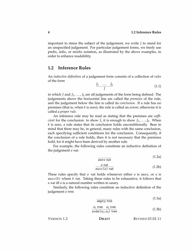
For example, the following rules constitute an inductive definition ofthe judgement a nat:
zero nat(1.2a)
a natsucc(a) nat
(1.2b)
These rules specify that a nat holds whenever either a is zero, or a issucc(b) where b nat. Taking these rules to be exhaustive, it follows thata nat iff a is a natural number written in unary.
Similarly, the following rules constitute an inductive definition of thejudgement a tree:
empty tree(1.3a)
a1 tree a2 treenode(a1; a2) tree
(1.3b)
VERSION 1.2 DRAFT REVISED 03.02.11
1.3 Derivations 5
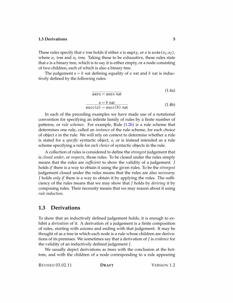
These rules specify that a tree holds if either a is empty, or a is node(a1; a2),where a1 tree and a2 tree. Taking these to be exhaustive, these rules statethat a is a binary tree, which is to say it is either empty, or a node consistingof two children, each of which is also a binary tree.
The judgement a = b nat defining equality of a nat and b nat is induc-tively defined by the following rules:
zero= zero nat(1.4a)
a = b natsucc(a)= succ(b) nat
(1.4b)
In each of the preceding examples we have made use of a notationalconvention for specifying an infinite family of rules by a finite number ofpatterns, or rule schemes. For example, Rule (1.2b) is a rule scheme thatdetermines one rule, called an instance of the rule scheme, for each choiceof object a in the rule. We will rely on context to determine whether a ruleis stated for a specific syntactic object, a, or is instead intended as a rulescheme specifying a rule for each choice of syntactic objects in the rule.
A collection of rules is considered to define the strongest judgement thatis closed under, or respects, those rules. To be closed under the rules simplymeans that the rules are sufficient to show the validity of a judgement: Jholds if there is a way to obtain it using the given rules. To be the strongestjudgement closed under the rules means that the rules are also necessary:J holds only if there is a way to obtain it by applying the rules. The suffi-ciency of the rules means that we may show that J holds by deriving it bycomposing rules. Their necessity means that we may reason about it usingrule induction.
1.3 Derivations
To show that an inductively defined judgement holds, it is enough to ex-hibit a derivation of it. A derivation of a judgement is a finite compositionof rules, starting with axioms and ending with that judgement. It may bethought of as a tree in which each node is a rule whose children are deriva-tions of its premises. We sometimes say that a derivation of J is evidence forthe validity of an inductively defined judgement J.
We usually depict derivations as trees with the conclusion at the bot-tom, and with the children of a node corresponding to a rule appearing
REVISED 03.02.11 DRAFT VERSION 1.2
6 1.3 Derivations
above it as evidence for the premises of that rule. Thus, if
J1 . . . JkJ
is an inference rule and #1, . . . ,#k are derivations of its premises, then
#1 . . . #kJ (1.5)
is a derivation of its conclusion. In particular, if k = 0, then the node has nochildren.
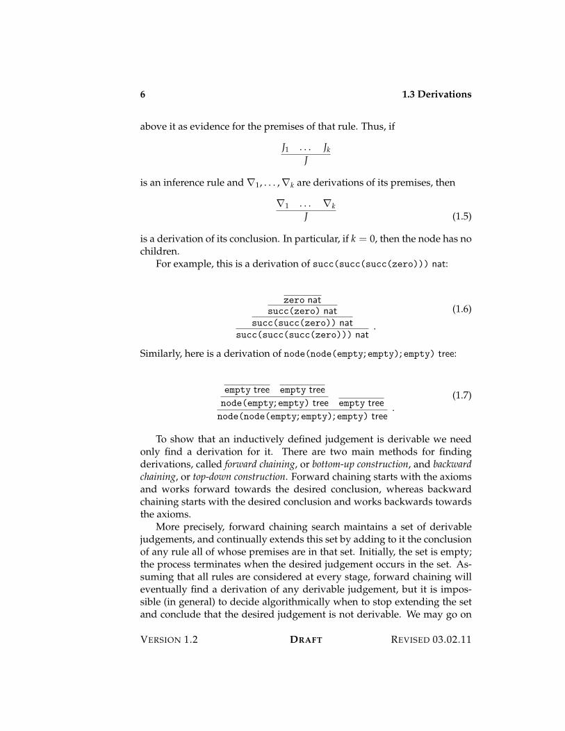
For example, this is a derivation of succ(succ(succ(zero))) nat:
zero natsucc(zero) nat
succ(succ(zero)) natsucc(succ(succ(zero))) nat
.
(1.6)
Similarly, here is a derivation of node(node(empty; empty); empty) tree:
empty tree empty treenode(empty; empty) tree empty treenode(node(empty; empty); empty) tree
.(1.7)
To show that an inductively defined judgement is derivable we needonly find a derivation for it. There are two main methods for findingderivations, called forward chaining, or bottom-up construction, and backwardchaining, or top-down construction. Forward chaining starts with the axiomsand works forward towards the desired conclusion, whereas backwardchaining starts with the desired conclusion and works backwards towardsthe axioms.
More precisely, forward chaining search maintains a set of derivablejudgements, and continually extends this set by adding to it the conclusionof any rule all of whose premises are in that set. Initially, the set is empty;the process terminates when the desired judgement occurs in the set. As-suming that all rules are considered at every stage, forward chaining willeventually find a derivation of any derivable judgement, but it is impos-sible (in general) to decide algorithmically when to stop extending the setand conclude that the desired judgement is not derivable. We may go on
VERSION 1.2 DRAFT REVISED 03.02.11
1.4 Rule Induction 7
and on adding more judgements to the derivable set without ever achiev-ing the intended goal. It is a matter of understanding the global propertiesof the rules to determine that a given judgement is not derivable.
Forward chaining is undirected in the sense that it does not take ac-count of the end goal when deciding how to proceed at each step. Incontrast, backward chaining is goal-directed. Backward chaining searchmaintains a queue of current goals, judgements whose derivations are tobe sought. Initially, this set consists solely of the judgement we wish to de-rive. At each stage, we remove a judgement from the queue, and considerall rules whose conclusion is that judgement. For each such rule, we addthe premises of that rule to the back of the queue, and continue. If there ismore than one such rule, this process must be repeated, with the same start-ing queue, for each candidate rule. The process terminates whenever thequeue is empty, all goals having been achieved; any pending considerationof candidate rules along the way may be discarded. As with forward chain-ing, backward chaining will eventually find a derivation of any derivablejudgement, but there is, in general, no algorithmic method for determiningin general whether the current goal is derivable. If it is not, we may futilelyadd more and more judgements to the goal set, never reaching a point atwhich all goals have been satisfied.
1.4 Rule Induction
Since an inductive definition specifies the strongest judgement closed un-der a collection of rules, we may reason about them by rule induction. Theprinciple of rule induction states that to show that a property P holds of ajudgement J whenever J is derivable, it is enough to show that P is closedunder, or respects, the rules defining J. Writing P(J) to mean that the prop-erty P holds of the judgement J, we say that P respects the rule
J1 . . . JkJ
if P(J) holds whenever P(J1), . . . , P(Jk). The assumptions P(J1), . . . , P(Jk)are called the inductive hypotheses, and P(J) is called the inductive conclusion,of the inference.
The principle of rule induction is simply the expression of the defini-tion of an inductively defined judgement form as the strongest judgementform closed under the rules comprising the definition. This means thatthe judgement form defined by a set of rules is both (a) closed under those
REVISED 03.02.11 DRAFT VERSION 1.2
8 1.4 Rule Induction
rules, and (b) sufficient for any other property also closed under those rules.The former means that a derivation is evidence for the validity of a judge-ment; the latter means that we may reason about an inductively definedjudgement form by rule induction.
To show that P(J) holds whenever J is derivable, it is often helpful toshow that the conjunction of P with J itself is closed under the rules. Thisis because one gets as an inductive hypotheses not only that P(Ji) holds foreach premise Ji, but also that Ji is derivable. Of course the inductive stepmust correspondingly show both that P(J), but also that J is derivable.But the latter requirement is immediately satisfied by an application of therule in question, whose premises are derivable by the inductive hypothesis.Having shown that the conjunction of P with J is closed under each of therules, it follows that if J is derivable, then we have both that P(J), and alsothat J is derivable, and we can just ignore the redundant auxiliary result.In practice we shall often tacitly employ this maneuver, only showing thata property is closed when restricted to derivable judgements.
When specialized to Rules (1.2), the principle of rule induction statesthat to show P(a nat) whenever a nat, it is enough to show:
1. P(zero nat).
2. for every a, if a nat and P(a nat), then (succ(a) nat and) P(succ(a) nat).
This is just the familiar principle of mathematical induction arising as a spe-cial case of rule induction. The first condition is called the basis of the in-duction, and the second is called the inductive step.
Similarly, rule induction for Rules (1.3) states that to show P(a tree)whenever a tree, it is enough to show
1. P(empty tree).
2. for every a1 and a2, if a1 tree and P(a1 tree), and if a2 tree and P(a2 tree),then (node(a1; a2) tree and) P(node(a1; a2) tree).
This is called the principle of tree induction, and is once again an instance ofrule induction.
As a simple example of a proof by rule induction, let us prove that nat-ural number equality as defined by Rules (1.4) is reflexive:
Lemma 1.1. If a nat, then a = a nat.
Proof. By rule induction on Rules (1.2):
VERSION 1.2 DRAFT REVISED 03.02.11
1.5 Iterated and Simultaneous Inductive Definitions 9
Rule (1.2a) Applying Rule (1.4a) we obtain zero= zero nat.
Rule (1.2b) Assume that a = a nat. It follows that succ(a)= succ(a) natby an application of Rule (1.4b).
As another example of the use of rule induction, we may show that thepredecessor of a natural number is also a natural number. While this mayseem self-evident, the point of the example is to show how to derive thisfrom first principles.
Lemma 1.2. If succ(a) nat, then a nat.
Proof. It suffices to show that the property, P(a nat) stating that a nat andthat a = succ(b) implies b nat is closed under Rules (1.2).
Rule (1.2a) Clearly zero nat, and the second condition holds vacuously,since zero is not of the form succ($).
Rule (1.2b) Inductively we know that a nat and that if a is of the formsucc(b), then b nat. We are to show that succ(a) nat, which is imme-diate, and that if succ(a) is of the form succ(b), then b nat, and wehave b nat by the inductive hypothesis.
This completes the proof.
Similarly, let us show that the successor operation is injective.
Lemma 1.3. If succ(a1)= succ(a2) nat, then a1 = a2 nat.
Proof. Similar to the proof of Lemma 1.2.
1.5 Iterated and Simultaneous Inductive Definitions
Inductive definitions are often iterated, meaning that one inductive defi-nition builds on top of another. In an iterated inductive definition thepremises of a rule
J1 . . . JkJ
REVISED 03.02.11 DRAFT VERSION 1.2
10 1.5 Iterated and Simultaneous Inductive Definitions
may be instances of either a previously defined judgement form, or thejudgement form being defined. For example, the following rules define thejudgement a list stating that a is a list of natural numbers.
nil list(1.8a)
a nat b listcons(a; b) list
(1.8b)
The first premise of Rule (1.8b) is an instance of the judgement form a nat,which was defined previously, whereas the premise b list is an instance ofthe judgement form being defined by these rules.
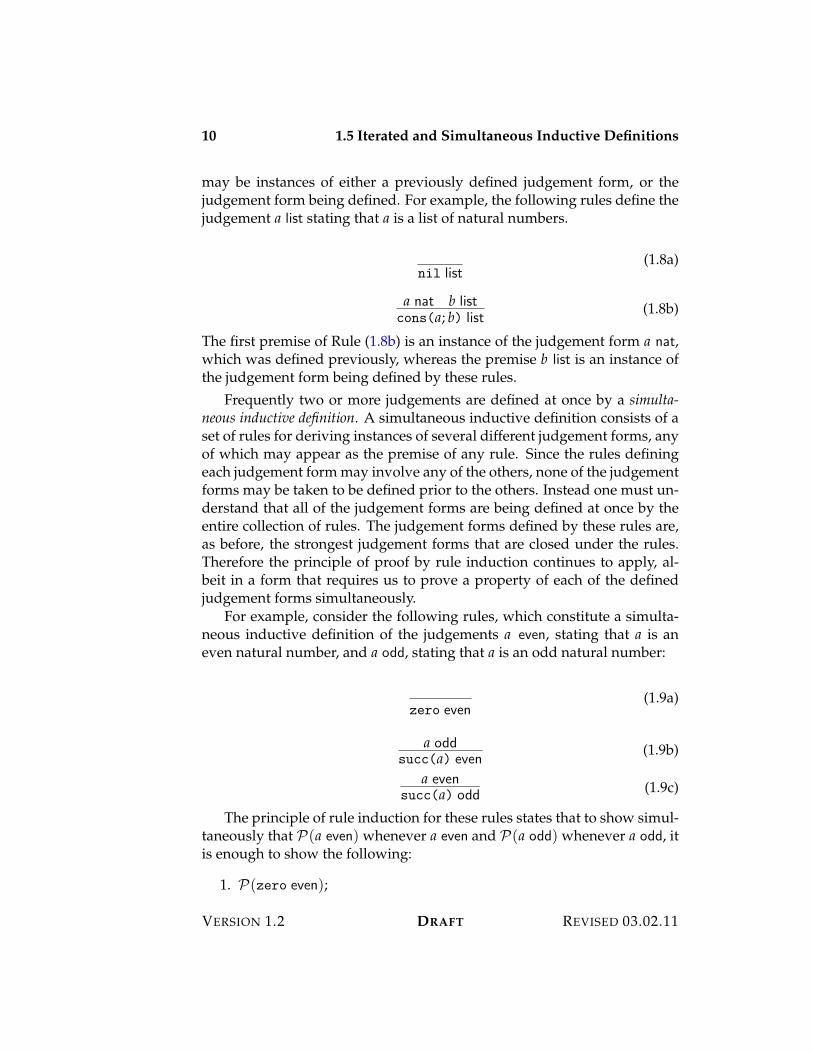
Frequently two or more judgements are defined at once by a simulta-neous inductive definition. A simultaneous inductive definition consists of aset of rules for deriving instances of several different judgement forms, anyof which may appear as the premise of any rule. Since the rules definingeach judgement form may involve any of the others, none of the judgementforms may be taken to be defined prior to the others. Instead one must un-derstand that all of the judgement forms are being defined at once by theentire collection of rules. The judgement forms defined by these rules are,as before, the strongest judgement forms that are closed under the rules.Therefore the principle of proof by rule induction continues to apply, al-beit in a form that requires us to prove a property of each of the definedjudgement forms simultaneously.
For example, consider the following rules, which constitute a simulta-neous inductive definition of the judgements a even, stating that a is aneven natural number, and a odd, stating that a is an odd natural number:
zero even(1.9a)
a oddsucc(a) even
(1.9b)
a evensucc(a) odd (1.9c)
The principle of rule induction for these rules states that to show simul-taneously that P(a even) whenever a even and P(a odd) whenever a odd, itis enough to show the following:
1. P(zero even);
VERSION 1.2 DRAFT REVISED 03.02.11
1.6 Defining Functions by Rules 11
2. if P(a odd), then P(succ(a) even);
3. if P(a even), then P(succ(a) odd).
As a simple example, we may use simultaneous rule induction to provethat (1) if a even, then a nat, and (2) if a odd, then a nat. That is, we definethe property P by (1) P(a even) iff a nat, and (2) P(a odd) iff a nat. Theprinciple of rule induction for Rules (1.9) states that it is sufficient to showthe following facts:
1. zero nat, which is derivable by Rule (1.2a).
2. If a nat, then succ(a) nat, which is derivable by Rule (1.2b).
3. If a nat, then succ(a) nat, which is also derivable by Rule (1.2b).
1.6 Defining Functions by Rules
A common use of inductive definitions is to define a function by giving aninductive definition of its graph relating inputs to outputs, and then show-ing that the relation uniquely determines the outputs for given inputs. Forexample, we may define the addition function on natural numbers as therelation sum(a; b; c), with the intended meaning that c is the sum of a and b,as follows:
b natsum(zero; b; b) (1.10a)
sum(a; b; c)sum(succ(a); b; succ(c))
(1.10b)
The rules define a ternary (three-place) relation, sum(a; b; c), among naturalnumbers a, b, and c. We may show that c is determined by a and b in thisrelation.
Theorem 1.4. For every a nat and b nat, there exists a unique c nat such thatsum(a; b; c).
Proof. The proof decomposes into two parts:
1. (Existence) If a nat and b nat, then there exists c nat such that sum(a; b; c).
2. (Uniqueness) If a nat, b nat, c nat, c% nat, sum(a; b; c), and sum(a; b; c%),then c = c% nat.
REVISED 03.02.11 DRAFT VERSION 1.2
12 1.7 Modes
For existence, let P(a nat) be the proposition if b nat then there exists c natsuch that sum(a; b; c). We prove that if a nat then P(a nat) by rule inductionon Rules (1.2). We have two cases to consider:
Rule (1.2a) We are to show P(zero nat). Assuming b nat and taking c tobe b, we obtain sum(zero; b; c) by Rule (1.10a).
Rule (1.2b) Assuming P(a nat), we are to show P(succ(a) nat). That is,we assume that if b nat then there exists c such that sum(a; b; c), andare to show that if b% nat, then there exists c% such that sum(succ(a); b%; c%).To this end, suppose that b% nat. Then by induction there exists c suchthat sum(a; b%; c). Taking c% = succ(c), and applying Rule (1.10b), weobtain sum(succ(a); b%; c%), as required.
For uniqueness, we prove that if sum(a; b; c1), then if sum(a; b; c2), then c1 = c2 natby rule induction based on Rules (1.10).
Rule (1.10a) We have a = zero and c1 = b. By an inner induction onthe same rules, we may show that if sum(zero; b; c2), then c2 is b. ByLemma 1.1 on page 8 we obtain b = b nat.
Rule (1.10b) We have that a = succ(a%) and c1 = succ(c%1), where sum(a%; b; c%1).By an inner induction on the same rules, we may show that if sum(a; b; c2),then c2 = succ(c%2) nat where sum(a%; b; c%2). By the outer inductive hy-pothesis c%1 = c%2 nat and so c1 = c2 nat.
1.7 Modes
The statement that one or more arguments of a judgement is (perhaps uniquely)determined by its other arguments is called a mode specification for thatjudgement. For example, we have shown that every two natural numbershave a sum according to Rules (1.10). This fact may be restated as a modespecification by saying that the judgement sum(a; b; c) has mode (&, &, ').The notation arises from the form of the proposition it expresses: for alla nat and for all b nat, there exists c nat such that sum(a; b; c). If we wishto further specify that c is uniquely determined by a and b, we would saythat the judgement sum(a; b; c) has mode (&, &, '!), corresponding to theproposition for all a nat and for all b nat, there exists a unique c nat such thatsum(a; b; c). If we wish only to specify that the sum is unique, if it exists,
VERSION 1.2 DRAFT REVISED 03.02.11
1.8 Exercises 13
then we would say that the addition judgement has mode (&, &, '(1), cor-responding to the proposition for all a nat and for all b nat there exists at mostone c nat such that sum(a; b; c).
As these examples illustrate, a given judgement may satisfy several dif-ferent mode specifications. In general the universally quantified argumentsare to be thought of as the inputs of the judgement, and the existentiallyquantified arguments are to be thought of as its outputs. We usually try toarrange things so that the outputs come after the inputs, but it is not es-sential that we do so. For example, addition also has the mode (&, '(1, &),stating that the sum and the first addend uniquely determine the secondaddend, if there is any such addend at all. Put in other terms, this says thataddition of natural numbers has a (partial) inverse, namely subtraction.We could equally well show that addition has mode ('(1, &, &), which isjust another way of stating that addition of natural numbers has a partialinverse.
Often there is an intended, or principal, mode of a given judgement,which we often foreshadow by our choice of notation. For example, whengiving an inductive definition of a function, we often use equations to in-dicate the intended input and output relationships. For example, we mayre-state the inductive definition of addition (given by Rules (1.10)) usingequations:
a nata + zero= a nat (1.11a)
a + b = c nata + succ(b)= succ(c) nat
(1.11b)
When using this notation we tacitly incur the obligation to prove that themode of the judgement is such that the object on the right-hand side of theequations is determined as a function of those on the left. Having done so,we abuse notation, writing a + b for the unique c such that a + b = c nat.
1.8 Exercises
1. Give an inductive definition of the judgement max(a; b; c), where a nat,b nat, and c nat, with the meaning that c is the larger of a and b. Provethat this judgement has the mode (&, &, '!).
2. Consider the following rules, which define the height of a binary treeas the judgement hgt(a; b).
hgt(empty; zero)(1.12a)
REVISED 03.02.11 DRAFT VERSION 1.2
14 1.8 Exercises
hgt(a1; b1) hgt(a2; b2) max(b1; b2; b)hgt(node(a1; a2); succ(b))
(1.12b)
Prove by tree induction that the judgement hgt has the mode (&, '),with inputs being binary trees and outputs being natural numbers.
3. Give an inductive definition of the judgement “# is a derivation of J”for an inductively defined judgement J of your choice.
4. Give an inductive definition of the forward-chaining and backward-chaining search strategies.
VERSION 1.2 DRAFT REVISED 03.02.11
Chapter 2
Hypothetical Judgements
A hypothetical judgement expresses an entailment between one or more hy-potheses and a conclusion. We will consider two notions of entailment, calledderivability and admissibility. Derivability expresses the stronger of the twoforms of entailment, namely that the conclusion may be deduced directlyfrom the hypotheses by composing rules. Admissibility expresses the weakerform, that the conclusion is derivable from the rules whenever the hypothe-ses are also derivable. Both forms of entailment enjoy the same structuralproperties that characterize conditional reasoning. One consequence ofthese properties is that derivability is stronger than admissibility (but theconverse fails, in general). We then generalize the concept of an inductivedefinition to admit rules that have hypothetical judgements as premises.Using these we may enrich the rules with new axioms that are available foruse within a specified premise of a rule.
2.1 Derivability
For a given set, R, of rules, we define the derivability judgement, writtenJ1, . . . , Jk )R K, where each Ji and K are basic judgements, to mean thatwe may derive K from the expansion R[J1, . . . , Jk] of the rules R with theadditional axioms
J1. . .
Jk.
That is, we treat the hypotheses, or antecedents, of the judgement, J1, . . . , Jnas temporary axioms, and derive the conclusion, or consequent, by composingrules in R. That is, evidence for a hypothetical judgement consists of aderivation of the conclusion from the hypotheses using the rules in R.
16 2.1 Derivability
We use capital Greek letters, frequently ! or ", to stand for a finite col-lection of basic judgements, and write R[!] for the expansion of R withan axiom corresponding to each judgement in !. The judgement ! )R Kmeans that K is derivable from rules R[!]. We sometimes write )R ! tomean that )R J for each judgement J in !. The derivability judgementJ1, . . . , Jn )R J is sometimes expressed by saying that the rule
J1 . . . JnJ (2.1)
is derivable from the rules R.For example, consider the derivability judgement
a nat )(1.2) succ(succ(a)) nat (2.2)
relative to Rules (1.2). This judgement is valid for any choice of object a, asevidenced by the derivation
a natsucc(a) nat
succ(succ(a)) nat, (2.3)
which composes Rules (1.2), starting with a nat as an axiom, and endingwith succ(succ(a)) nat. Equivalently, the validity of (2.2) may also beexpressed by stating that the rule
a natsucc(succ(a)) nat
(2.4)
is derivable from Rules (1.2).It follows directly from the definition of derivability that it is stable un-
der extension with new rules.
Theorem 2.1 (Stability). If ! )R J, then ! )R*R% J.
Proof. Any derivation of J from R[!] is also a derivation from (R *R %)[!],since any rule in R is also a rule in R *R %.
Derivability enjoys a number of structural properties that follow from itsdefinition, independently of the rules, R, in question.
Reflexivity Every judgement is a consequence of itself: !, J )R J. Eachhypothesis justifies itself as conclusion.
VERSION 1.2 DRAFT REVISED 03.02.11
2.2 Admissibility 17
Weakening If ! )R J, then !, K )R J. Entailment is not influenced byunexercised options.
Transitivity If !, K )R J and ! )R K, then ! )R J. If we replace an ax-iom by a derivation of it, the result is a derivation of its consequentwithout that hypothesis.
Reflexivity follows directly from the meaning of derivability. Weakeningfollows directly from the definition of derivability. Transitivity is provedby rule induction on the first premise.
2.2 Admissibility
Admissibility, written ! |=R J, is a weaker form of hypothetical judgementstating that )R ! implies )R J. That is, the conclusion J is derivable fromrules R whenever the assumptions ! are all derivable from rules R. Inparticular if any of the hypotheses are not derivable relative to R, then thejudgement is vacuously true. The admissibility judgement J1, . . . , Jn |=R Jis sometimes expressed by stating that the rule,
J1 . . . JnJ
,(2.5)
is admissible relative to the rules in R.For example, the admissibility judgement
succ(a) nat |=(1.2) a nat (2.6)
is valid, because any derivation of succ(a) nat from Rules (1.2) must con-tain a sub-derivation of a nat from the same rules, which justifies the con-clusion. The validity of (2.6) may equivalently be expressed by stating thatthe rule
succ(a) nata nat (2.7)
is admissible for Rules (1.2).In contrast to derivability the admissibility judgement is not stable un-
der extension to the rules. For example, if we enrich Rules (1.2) with theaxiom
succ(junk) nat(2.8)
REVISED 03.02.11 DRAFT VERSION 1.2
18 2.2 Admissibility
(where junk is some object for which junk nat is not derivable), then theadmissibility (2.6) is invalid. This is because Rule (2.8) has no premises,and there is no composition of rules deriving junk nat. Admissibility is assensitive to which rules are absent from an inductive definition as it is towhich rules are present in it.
The structural properties of derivability ensure that derivability is strongerthan admissibility.
Theorem 2.2. If ! )R J, then ! |=R J.
Proof. Repeated application of the transitivity of derivability shows that if! )R J and )R !, then )R J.
To see that the converse fails, observe that there is no composition ofrules such that
succ(junk) nat )(1.2) junk nat,
yet the admissibility judgement
succ(junk) nat |=(1.2) junk nat
holds vacuously.Evidence for admissibility may be thought of as a mathematical func-
tion transforming derivations #1, . . . ,#n of the hypotheses into a deriva-tion # of the consequent. Therefore, the admissibility judgement enjoysthe same structural properties as derivability, and hence is a form of hypo-thetical judgement:
Reflexivity If J is derivable from the original rules, then J is derivable fromthe original rules: J |=R J.
Weakening If J is derivable from the original rules assuming that each ofthe judgements in ! are derivable from these rules, then J must also bederivable assuming that ! and also K are derivable from the originalrules: if ! |=R J, then !, K |=R J.
Transitivity If !, K |=R J and ! |=R K, then ! |=R J. If the judgements in! are derivable, so is K, by assumption, and hence so are the judge-ments in !, K, and hence so is J.
Theorem 2.3. The admissibility judgement ! |=R J is structural.
VERSION 1.2 DRAFT REVISED 03.02.11
2.3 Hypothetical Inductive Definitions 19
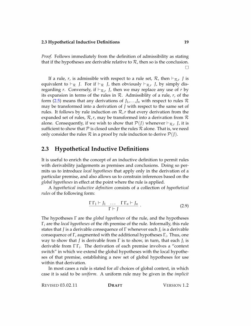
Proof. Follows immediately from the definition of admissibility as statingthat if the hypotheses are derivable relative to R, then so is the conclusion.
If a rule, r, is admissible with respect to a rule set, R, then )R,r J isequivalent to )R J. For if )R J, then obviously )R,r J, by simply dis-regarding r. Conversely, if )R,r J, then we may replace any use of r byits expansion in terms of the rules in R. Admissiblity of a rule, r, of theform (2.5) means that any derivations of J1,. . . ,Jn with respect to rules Rmay be transformed into a derivation of J with respect to the same set ofrules. It follows by rule induction on R, r that every derivation from theexpanded set of rules, R, r, may be transformed into a derivation from Ralone. Consequently, if we wish to show that P(J) whenever )R,r J, it issufficient to show that P is closed under the rules R alone. That is, we needonly consider the rules R in a proof by rule induction to derive P(J).
2.3 Hypothetical Inductive Definitions
It is useful to enrich the concept of an inductive definition to permit ruleswith derivability judgements as premises and conclusions. Doing so per-mits us to introduce local hypotheses that apply only in the derivation of aparticular premise, and also allows us to constrain inferences based on theglobal hypotheses in effect at the point where the rule is applied.
A hypothetical inductive definition consists of a collection of hypotheticalrules of the following form:
! !1 ) J1 . . . ! !n ) Jn! ) J
. (2.9)
The hypotheses ! are the global hypotheses of the rule, and the hypotheses!i are the local hypotheses of the ith premise of the rule. Informally, this rulestates that J is a derivable consequence of ! whenever each Ji is a derivableconsequence of !, augmented with the additional hypotheses !i. Thus, oneway to show that J is derivable from ! is to show, in turn, that each Ji isderivable from ! !i. The derivation of each premise involves a “contextswitch” in which we extend the global hypotheses with the local hypothe-ses of that premise, establishing a new set of global hypotheses for usewithin that derivation.
In most cases a rule is stated for all choices of global context, in whichcase it is said to be uniform. A uniform rule may be given in the implicit
REVISED 03.02.11 DRAFT VERSION 1.2
20 2.3 Hypothetical Inductive Definitions
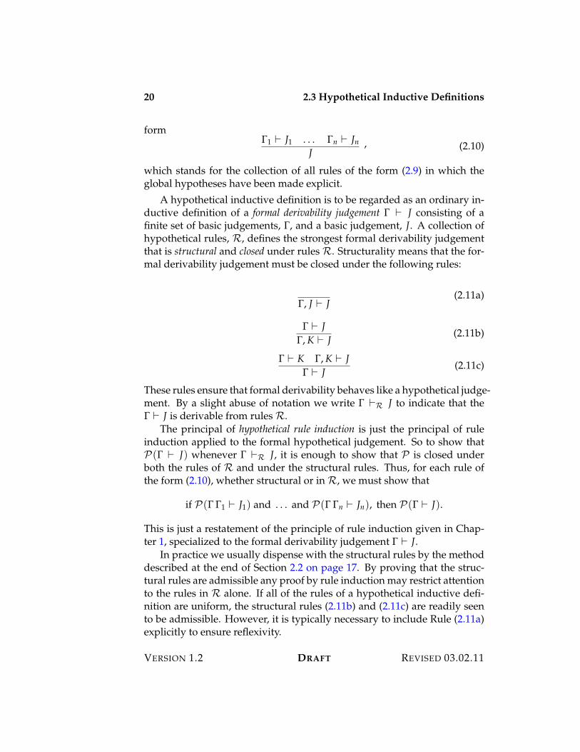
form!1 ) J1 . . . !n ) Jn
J, (2.10)
which stands for the collection of all rules of the form (2.9) in which theglobal hypotheses have been made explicit.
A hypothetical inductive definition is to be regarded as an ordinary in-ductive definition of a formal derivability judgement ! ) J consisting of afinite set of basic judgements, !, and a basic judgement, J. A collection ofhypothetical rules, R, defines the strongest formal derivability judgementthat is structural and closed under rules R. Structurality means that the for-mal derivability judgement must be closed under the following rules:
!, J ) J(2.11a)
! ) J!, K ) J
(2.11b)
! ) K !, K ) J! ) J
(2.11c)
These rules ensure that formal derivability behaves like a hypothetical judge-ment. By a slight abuse of notation we write ! )R J to indicate that the! ) J is derivable from rules R.
The principal of hypothetical rule induction is just the principal of ruleinduction applied to the formal hypothetical judgement. So to show thatP(! ) J) whenever ! )R J, it is enough to show that P is closed underboth the rules of R and under the structural rules. Thus, for each rule ofthe form (2.10), whether structural or in R, we must show that
if P(! !1 ) J1) and . . . and P(! !n ) Jn), then P(! ) J).
This is just a restatement of the principle of rule induction given in Chap-ter 1, specialized to the formal derivability judgement ! ) J.
In practice we usually dispense with the structural rules by the methoddescribed at the end of Section 2.2 on page 17. By proving that the struc-tural rules are admissible any proof by rule induction may restrict attentionto the rules in R alone. If all of the rules of a hypothetical inductive defi-nition are uniform, the structural rules (2.11b) and (2.11c) are readily seento be admissible. However, it is typically necessary to include Rule (2.11a)explicitly to ensure reflexivity.
VERSION 1.2 DRAFT REVISED 03.02.11
2.4 Exercises 21
2.4 Exercises
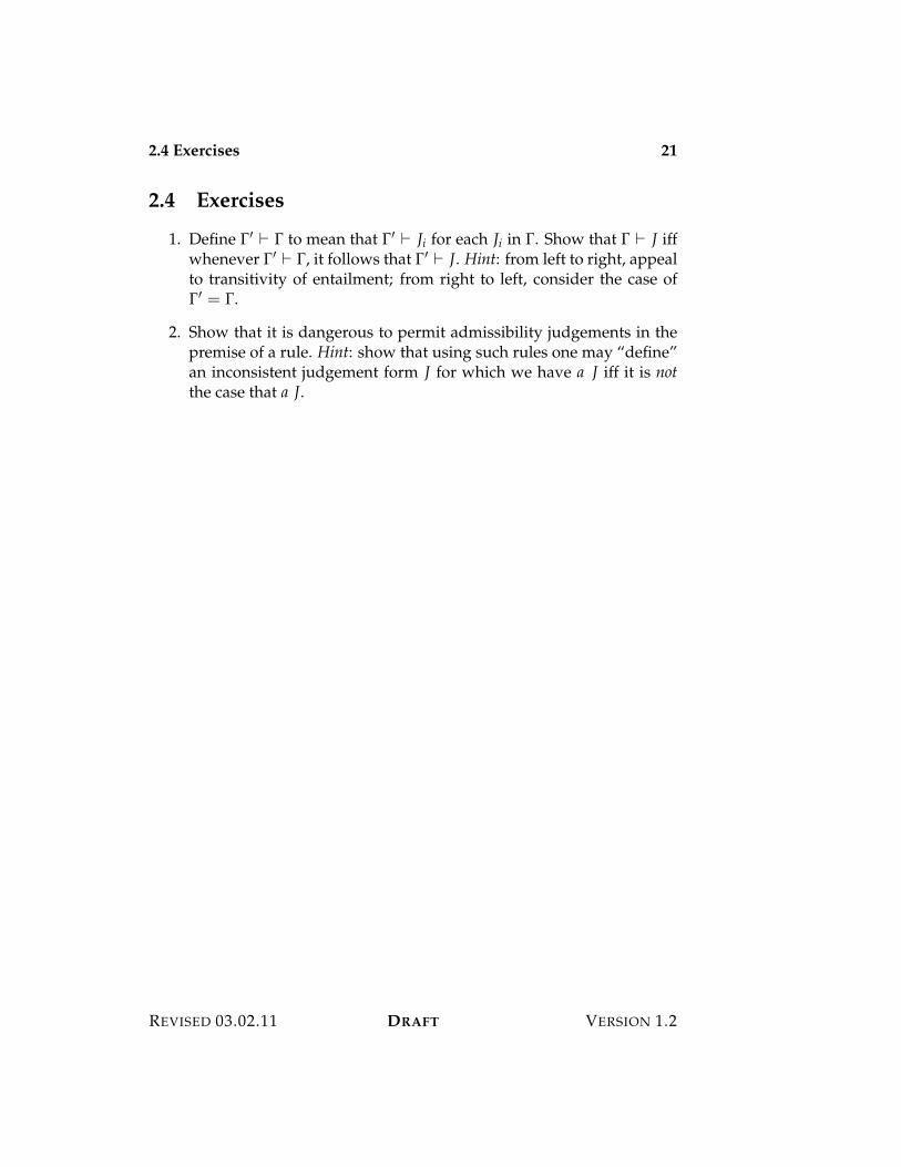
1. Define !% ) ! to mean that !% ) Ji for each Ji in !. Show that ! ) J iffwhenever !% ) !, it follows that !% ) J. Hint: from left to right, appealto transitivity of entailment; from right to left, consider the case of!% = !.
2. Show that it is dangerous to permit admissibility judgements in thepremise of a rule. Hint: show that using such rules one may “define”an inconsistent judgement form J for which we have a J iff it is notthe case that a J.
REVISED 03.02.11 DRAFT VERSION 1.2

22 2.4 Exercises
VERSION 1.2 DRAFT REVISED 03.02.11
Chapter 3
Syntax Trees
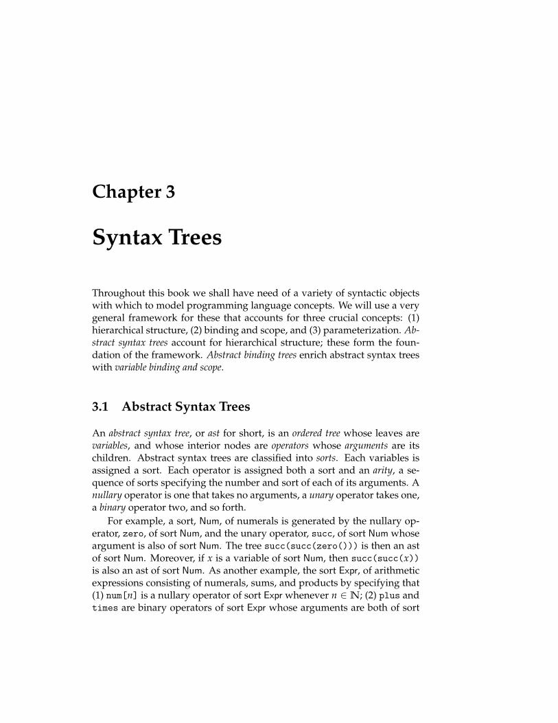
Throughout this book we shall have need of a variety of syntactic objectswith which to model programming language concepts. We will use a verygeneral framework for these that accounts for three crucial concepts: (1)hierarchical structure, (2) binding and scope, and (3) parameterization. Ab-stract syntax trees account for hierarchical structure; these form the foun-dation of the framework. Abstract binding trees enrich abstract syntax treeswith variable binding and scope.
3.1 Abstract Syntax Trees
An abstract syntax tree, or ast for short, is an ordered tree whose leaves arevariables, and whose interior nodes are operators whose arguments are itschildren. Abstract syntax trees are classified into sorts. Each variables isassigned a sort. Each operator is assigned both a sort and an arity, a se-quence of sorts specifying the number and sort of each of its arguments. Anullary operator is one that takes no arguments, a unary operator takes one,a binary operator two, and so forth.
For example, a sort, Num, of numerals is generated by the nullary op-erator, zero, of sort Num, and the unary operator, succ, of sort Num whoseargument is also of sort Num. The tree succ(succ(zero())) is then an astof sort Num. Moreover, if x is a variable of sort Num, then succ(succ(x))is also an ast of sort Num. As another example, the sort Expr, of arithmeticexpressions consisting of numerals, sums, and products by specifying that(1) num[n] is a nullary operator of sort Expr whenever n + N; (2) plus andtimes are binary operators of sort Expr whose arguments are both of sort

24 3.1 Abstract Syntax Trees
Expr. Thenplus(num[2]; times(num[3]; x))
is an ast of sort Expr, assuming that x is a variable of the same sort.In general a collection of abstract syntax trees is specified by two pieces
of data. First, we must specify a finite set, S , of sorts. This determinesthe categories of syntax in the language under consideration. Second, foreach sort s + S , we specify a set, Os, of operators of sort s, and define foreach such operator, o, its arity, ar(o) = (s1, . . . , sn), which determines thenumber and sorts of its arguments. We also assume that for each sort s + Sthere is an infinite set, Xs, of variables of sort s that are distinct from any ofthe operators (so that there can be no ambiguity about what is a variable).
Given this data, the S-indexed family A[X ] = {A[X ]s }s+S of abstractsyntax trees is inductively defined by the following conditions:
1. A variable of sort s is an ast of sort s: if x + Xs, then x + A[X ]s.
2. Compound ast’s are formed by operators: if ar(o) = (s1, . . . , sn), anda1 + A[X ]s1 , . . . , an + A[X ]sn , then o(a1; . . . ;an) + A[X ]s.
We will often use notational conventions to identify the variables of asort, and speak loosely of an “ast of sort s” without precisely specifying thesets of variables of each sort. When specifying the variables, we often writeX , x, where x is a variable of sort s such that x /+ Xs, to mean the family ofsets Y such that Ys = Xs * { x } and Ys% = Xs% for all s% ,= s. The familyX , x, where x is of sort s, is said to be the family obtained by adjoining thevariable x to the family X .
It is easy to see that if X - Y , then A[X ] - A[Y ].1 A S-indexedfamily of bijections # : X . Y between variables2 induces a renaming,# · a, on a + A[X ] yielding an ast in A[Y ] obtained by replacing x + Xsby #s(x) everywhere in a. (Renamings will play an important role in thegeneralization of ast’s to account for binding and scope to be developed inSection 3.2 on the next page.)
Variables are given meaning by substitution: a variable stands for anast to be determined later. More precisely, if a + A[X , x] and b + A[X ],then [b/x]a + A[X ], where [b/x]a is the result of substituting b for everyoccurrence of x in a. The ast a is sometimes called the target, and x is calledthe subject, of the substitution. Substitution is defined by the followingconditions:
1Relations on sets extend to relations on families of sets element-wise, so that X - Ymeans that for every s + S , Xs - Ys.
2That is, #s : Xs . Ys for each s + S .
VERSION 1.2 DRAFT REVISED 03.02.11
3.2 Abstract Binding Trees 25
1. [b/x]x = b and [b/x]y = y if x ,= y.
2. [b/x]o(a1; . . . ;an) = o([b/x]a1; . . . ;[b/x]an).
For example, we may readily check that
[succ(zero())/x]succ(succ(x)) = succ(succ(succ(zero()))).
Substitution simply “plugs in” the given subject for a specified variable inthe target.
To prove that a property, P , holds of a class of abstract syntax trees wemay use the principle of structural induction, or induction on syntax. To showthat A[X ] - P , it is enough to show:
1. X - P .
2. if ar(o) = (s1, . . . , sn), if a1 + Ps1 and . . . and an + Psn , then o(a1; . . . ;an) +Ps.
That is, to show that every ast of sort s has property Ps, it is enough toshow that every variable of sort s has the property Ps and that for everyoperator o of sort s whose arguments have sorts s1, . . . , sn, respectively, if a1has property Ps1 , and . . . and an has property Psn , then o(a1; . . . ;an) hasproperty Ps.
For example, we may prove by structural induction that substitution onast’s is well-defined.
Theorem 3.1. If b + A[X ], then for every b + A[X ] there exists a uniquec + A[X ] such that [b/x]a = c
Proof. By structural induction on a. If a = x, then c = b by definition,otherwise if a = y ,= x, then c = y, also by definition. Otherwise, a =o(a1, . . . , an), and we have by induction unique c1, . . . , cn such that [b/x]a1 =c1 and . . . [b/x]an = cn, and so c is c = o(c1; . . . ;cn), by definition of sub-stitution.
3.2 Abstract Binding Trees
Abstract syntax goes a long way towards separating objective issues of syn-tax (the hierarchical structure of expressions) from subjective issues (theirlayout on the page). This can be usefully pushed a bit further by enrichingabstract syntax to account for binding and scope.
REVISED 03.02.11 DRAFT VERSION 1.2
26 3.2 Abstract Binding Trees
All languages have facilities for introducing an identifier with a spec-ified range of significance. For example, we may define a variable, x, tostand for an expression, e1, so that we may conveniently refer to it withinanother expression, e2, by writing let x be e1 in e2. The intention is that xstands for e1 inside of the expression e2, but has no meaning whatsoeveroutside of that expression. The variable x is said to be bound within e2 by thedefinition; equivalently, the scope of the variable x is the expression e2.
Moreover, the name x has no intrinsic significance; we may just as welluse any variable y for the same purpose, provided that we rename x to ywithin e2. Such a renaming is always possible, provided only that there canbe no confusion between two different definitions. So, for example, there isno difference between the expressions
let x be succ(succ(zero)) in succ(succ(x))
andlet y be succ(succ(zero)) in succ(succ(y)).
But we must be careful when nesting definitions, since
let x be succ(succ(zero)) in let y be succ(zero) in succ(x)
is entirely different from
let y be succ(succ(zero)) in let y be succ(zero) in succ(y).
In this case we cannot rename x to y, nor can we rename y to x, because todo so would confuse two different definitions. The guiding principle is thatbound variables are pointers to their binding sites, and that any renamingmust preserve the pointer structure of the expression. Put in other terms,bound variables function as pronouns, which refer to objects separately in-troduced by a noun phrase (here, an expression). Renaming must preservethe pronoun structure, so that we cannot get confusions such as “which hedo you mean?” that arise in less formal languages.
The concepts of binding and scope can be accounted by enriching ab-stract syntax trees with some additional structure. Such enriched abstractsyntax trees are called abstract binding trees, or abt’s for short. An opera-tor on abt’s may bind zero or more variables in each of its arguments in-dependently of one another. Each argument is an abstractor of the formx1, . . . , xk.a, where x1, . . . , xk are variables and a is an abt possibly mention-ing those variables. Such an abstractor specifies that the variables x1, . . . , xk
VERSION 1.2 DRAFT REVISED 03.02.11
3.2 Abstract Binding Trees 27
are bound within e2. When k is zero, we usually elide the distinction be-tween .a and a itself. Thus, when written in the form of an abt, a definitionhas the form let(e1; x.e2). The abstractor x.e2 in the second argumentposition makes clear that x is bound within e2, and not within e1.
Since an operator may bind variables in each of its arguments, the ar-ity of an operator is generalized to be a finite sequence of valences of theform (s1, . . . , sk)s consisting of a finite sequence of sorts together with asort. Such a valence specifies the overall sort of the argument, s, and thesorts s1, . . . , sk of the variables bound within that argument. Thus, for ex-ample, the arity of the operator let is (Expr, (Expr)Expr), which indicatesthat it takes two arguments described as follows:
1. The first argument is of sort Expr, and binds no variables.
2. The second argument is also of sort Expr, and binds one variable ofsort Expr.
A precise definition of abt’s requires some care. As a first approxima-tion let us naıvely define the S-indexed family B[X ] of abt’s over the S-indexed variables X and S-indexed family O of operators o of arity ar(o).To lighten the notation let us write!x for a finite sequence x1, . . . , xn of n dis-tinct variables, and!s for a finite sequence s1, . . . , sn of n sorts. We say that!x is a sequence of variables of sort !s iff the two sequences have the samelength, n, and for each 1 ( i ( n the variable xi is of sort si. The followingconditions would appear to suffice as the definition of the abt’s of each sort:
1. Every variable is an abt: X - B[X ].
2. Compound abt’s are formed by operators: if arity ((!s1)s1, . . . , (!sn)sn),and if !x1 is of sort!s1 and a1 + B[X ,!x1]s1 and . . . and !xn is of sort!snand an + B[X ,!xn]sn , then o(!x1.a1; . . . ;!xn.an) + B[X ]s.
The bound variables are adjoined to the set of active variables within eachargument, with the sort of each variable determined by the valence of theoperator.
This definition is almost correct. The problem is that it takes too literallythe names of the bound variables in an ast. In particular an abt of the formlet(e1; x.let(e2; x.e3)) is always ill-formed according to this definition,because the first binding adjoins x to X , which implies that the secondcannot adjoin x to X , x because it is already present.
REVISED 03.02.11 DRAFT VERSION 1.2
28 3.2 Abstract Binding Trees
To ensure that the names of bound variables do not matter, the secondcondition on formation of abt’s is strengthened as follows:3
if for every 1 ( i ( n and for every renaming #i : !xi . !x%i suchthat !x%i /+ X we have #i · ai + B[X ,!x%i ], then
o(!x1.a1; . . . ;!xn.an) + B[X ].
That is, we demand that an abstractor be well-formed with respect to everychoice of variables that are not already active. This ensures, for example,that when nesting binders we rename bound variables to avoid collisions.This is called the freshness condition on binders, since it chooses the boundvariable names to be “fresh” relative to any variables already in use in agiven context.
The principle of structural induction extends to abt’s, and is called struc-tural induction modulo renaming. It states that to show that B[X ] - P [X ], itis enough to show the following conditions:
1. X - P [X ].
2. For every o of sort s and arity ((!s1)s1, . . . , (!sn)sn), if for every 1 ( i (n and for every renaming #i : !xi . !x%i we have #i · ai + P [X ,!x%i ], theno(!x1.a1; . . . ;!xn.an) + P [X ].
This means that in the inductive hypothesis we may assume that the prop-erty P holds for all renamings of the bound variables, provided only thatno confusion arises by re-using varaible names.
As an example let us define by structural induction modulo renamingthe relation x + a, where a + B[X , x], to mean that x occurs free in a.Speaking somewhat loosely, we may say that this judgement is defined bythe following conditions:
1. x + y if x = y.
2. x + o(!x1.a1; . . . ;!xn.an) if, for some 1 ( i ( n, x + # · ai for everyfresh renaming # : !xi . !zi.
More precisely, we are defining a family of relations x + a for each family Xof variables such that a + B[X , x]. The first condition condition states that
3The action of a renaming extends to abt’s in the obvious way by replacing every occur-rence of x by #(x), including any occurrences in the variable list of an abstractor as well aswithin its body.
VERSION 1.2 DRAFT REVISED 03.02.11
3.2 Abstract Binding Trees 29
x is free in x, but not free in y for any variable y other than x. The secondcondition states that if x is free in some argument regardless of the choice ofbound variables, then it is free in the abt constructed by an operator. Thisimplies, in particular, that x is not free in let(zero; x.x), since x is not freein z for any fresh choice of z, which is necessarily distinct from x.
The relation a =$ b of $-equivalence (so-called for historical reasons), isdefined to mean that a and b are identical up to the choice of bound variablenames. This relation is defined to be the strongest congruence containingthe following two conditions:
1. x =$ x.
2. o(!x1.a1; . . . ;!xn.an) =$ o(!x%1.a%1; . . . ;!x%n.a%n) if for every 1 ( i ( n,#i · ai =$ #%
i · a%i for all fresh renamings #i : !xi . !zi and #%i : !x%i . !zi.
The idea is that we rename !xi and !x%i consistently, avoiding confusion, andcheck that ai and a%i are $-equivalent. As a matter of terminology, if a =$ b,then b is said to be an $-variant of a (and vice-versa).
Some care is required in the definition of substitution of an abt b of sorts for free occurrences of a variable x of sort s in some abt a of some sort,written [b/x]a. Substitution is partially defined by the following conditions:
1. [b/x]x = b, and [b/x]y = y if x ,= y.
2. [b/x]o(!x1.a1; . . . ;!xn.an) = o(!x1.a%1; . . . ;!xn.a%n), where, for each 1 (i ( n, we require that !xi ,+ b, and we set a%i = [b/x]ai if x /+ !xi, anda%i = ai otherwise.
If x is bound in some argument to an operator, then substitution does notdescend into its scope, for to do so would be to confuse two distinct vari-ables. For this reason we must take care to define a%i in the second equationaccording to whether or not x + !xi. The requirement that !xi ,+ b in thesecond equation is called capture avoidance. If some xi,j occurred free in b,then the result of the substitution [b/x]ai would in general contain xi,j freeas well, but then forming !xi.[b/x]ai would incur capture by changing thereferent of xi,j to be the jth bound variable of the ith argument. In suchcases substitution is undefined since we cannot replace x by b in ai withoutincurring capture.
One way around this is to alter the definition of substitution so that thebound variables in the result are chosen fresh by substitution. By the prin-ciple of structural induction we know inductively that, for any renaming
REVISED 03.02.11 DRAFT VERSION 1.2
30 3.3 Parameterization
#i : !xi . !x%i with !x%i fresh, the substitution [b/x](#i · ai) is well-defined.Hence we may define
[b/x]o(!x1.a1; . . . ;!xn.an) = o(!x%1.[b/x](#1 · a1); . . . ;!x%n.[b/x](#n · an))
for some particular choice of fresh bound variable names (any choice willdo). There is no longer any need to take care that x /+ !xi in each argument,because the freshness condition on binders ensures that this cannot occur,the variable x already being active. Noting that
o(!x1.a1; . . . ;!xn.an) =$ o(!x%1.#1 · a1; . . . ;!x%n.#n · an),
another way to avoid undefined substitutions is to first choose an $-variantof the target of the substitution whose binders avoid any free variables inthe substituting abt, and then perform substitution without fear of incur-ring capture. In other words substitution is totally defined on $-equivalenceclasses of abt’s.
This motivates the following general policy:
Abstract binding trees are always to be identified up to $-equivalence.
That is, we henceforth work with equivalence classes of abt’s modulo $-equivalence. Whenever a particular abt is considered, we choose a conve-nient representative of its $-equivalence class so that its bound variables aredisjoint from the finite set of active variables in a particular context. We tac-itly assert that all operations and relations on abt’s respect $-equivalence,so that they are properly defined on $-equivalence classes of abt’s. Thus, inparticular, it makes no sense to speak of a particular bound variable withinan abt, because bound variables have no fixed identity. Whenever we ex-amine an abt, we are choosing a representative of its $-equivalence class,and we have no control over how the bound variable names are chosen.On the other hand experience shows that any operation or property of in-terest respects $-equivalence, so there is no obstacle to achieving it. Indeed,we might say that a property or operation is legitimate exactly insofar as itrespects $-equivalence!
3.3 Parameterization
It is often useful to consider indexed families of operators in which indicesrange over a fixed set given in advance. For example, earlier we consideredthe family of nullary operators numn of sort Expr, where n + N is a natu-ral number. As in this example, we shall generally use square brackets to
VERSION 1.2 DRAFT REVISED 03.02.11

3.3 Parameterization 31
mark the index of a family of operators, and round brackets to designateits arguments. For example, consider the family of operators seq[n] of sortExpr with arity
(Expr, . . . ,Expr! "# $n
).
Then seq[n](a1; . . . ; an) is an ast of sort Expr, provided that each ai is anast of the same sort.
Another form of indexing in which the index set of the family is notspecified in advance, but rather depends on the context of occurrence ofthe operator, arises frequently. Such operators are indexed by symbols (alsocalled names or atoms) that are introduced within a scope by a binder. Un-like variables, symbols are not given meaning by substitution; rather, theyserve solely as names for operators. In particular there is no notion of sub-stitution for symbols.
As an example, we might consider a family of nullary operators cls[a]of sort Expr indexed by symbols a. (Such an operator might represent aclass of data viewed as a form of expression; see Chapter 15 for further de-velopment of this idea.) Whether such an operator is available depends onwhether it occurs within the scope of the declaration of a. As new symbolsare introduced, new operators become available; as the scope of a symbolis exited, operators that depend on it may no longer be used.
To allow for scoped parameterization of operators, we enrich the con-cept of an abstract binding tree to include binding of symbols, as well asvariables. In addition to its sort, s, an operator may also have a sort, r, ofparameters, and has an arity of the form
((!r1;!s1)s1, . . . , (!rn;!sn)sn)
specifying that it takes n arguments of sort s1, . . . , sn, respectively, and bindsparameters of sorts!ri and variables of sorts!si in the ith argument position.The set B[U ;X ] of parameterized abt’s is inductively defined by the follow-ing conditions:
1. X - B[U ;X ].
2. If ar(o) = ((!r1;!s1)s1, . . . , (!rn;!sn)sn), u + Ur, a1 + B[U ,!u1;X ,!x1] and. . . and an + B[U ,!un;X ,!xn], then o[u](!u1.!x1.a1; . . . ;!un.!xn.an) +B[U ;X ].4
4More precisely, we must consider all possible fresh renamings of the bound parametersin a parameterized abt, just as we considered all possible fresh renamings of the boundvariables in the definition of an abt.
REVISED 03.02.11 DRAFT VERSION 1.2
32 3.4 Exercises
The principle of structural induction modulo renaming extends to param-eterized abt’s in such a way that the names of bound parameters may bechosen arbitrarily to be fresh, just as may the names of bound variables bechosen arbitrarily in the induction principle for abt’s. The relation of $-equivalence extends to parameterized abt’s in the evident manner, relatingany two abt’s that differ only in their choice of bound parameter names.As with abt’s, we tacitly identify parameterized abt’s up to this extendednotion of $-equivalence, and demand that all properties and operations onparameterized abt’s respect $-equivalence.
3.4 Exercises
1. Show that for every a + B[X , x], either x + a or x ,+ a by structuralinduction modulo renaming on a.
VERSION 1.2 DRAFT REVISED 03.02.11
Chapter 4
Generic Judgements
Basic judgements express properties of objects of the universe of discourse.Hypothetical judgements express entailments between judgements, or rea-soning under hypotheses. Generic and parametric judgements express gen-erality with respect to variables and parameters, respectively. Generic judge-ments are given meaning by substitution, whereas parametric judgementsexpress uniform dependence on parameters.
4.1 Rule Schemes
An inductive definition consists of a set, R, of rules whose premises andconclusion are judgements involving syntactic objects generated by givensets of parameters and variables. We write ! )U ;X
R J to indicate that J isderivable from rules R and hypotheses ! over the universe B[U ;X ]. Thus,for example, if a + B[U ;X ], then the judgment a nat ) succ(a) nat isderivable from Rules (1.2) by applying Rule (1.2b) to the hypothesis a nat.
This definition hides a subtle issue of the interpretation of rules. Whenworking over a fixed universe of syntactic objects, one may understand arule of the form
a natsucc(a) nat
(4.1)
as standing for an infinite set of rules, one for each choice of object a in theuniverse. However, when considering the same rule over many differentuniverses (for example, by expanding the set of variables), this rough-and-ready interpretation must be refined.
To allow for variation in the universe we regard (4.1) as a rule schemein which the meta-variable, a, stands for a syntactic object in any expansion
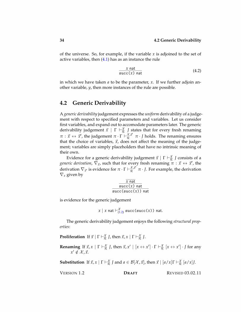
34 4.2 Generic Derivability
of the universe. So, for example, if the variable x is adjoined to the set ofactive variables, then (4.1) has as an instance the rule
x natsucc(x) nat
(4.2)
in which we have taken a to be the parameter, x. If we further adjoin an-other variable, y, then more instances of the rule are possible.
4.2 Generic Derivability
A generic derivability judgement expresses the uniform derivability of a judge-ment with respect to specified parameters and variables. Let us considerfirst variables, and expand out to accomodate parameters later. The genericderivability judgement !x | ! )X
R J states that for every fresh renaming# : !x . !x%, the judgement # · ! )X ,!x%
R # · J holds. The renaming ensuresthat the choice of variables, !x, does not affect the meaning of the judge-ment; variables are simply placeholders that have no intrinsic meaning oftheir own.
Evidence for a generic derivability judgement !x | ! )XR J consists of a
generic derivation, #!x, such that for every fresh renaming # : !x . !x%, thederivation #!x% is evidence for # · ! )X ,!x%
R # · J. For example, the derivation#x given by
x natsucc(x) nat
succ(succ(x)) nat
is evidence for the generic judgement
x | x nat )X(1.2) succ(succ(x)) nat.
The generic derivability judgement enjoys the following structural prop-erties:
Proliferation If !x | ! )XR J, then !x, x | ! )X
R J.
Renaming If !x, x | ! )XR J, then !x, x% | [x . x%] · ! )X
R [x . x%] · J for anyx% /+ X ,!x.
Substitution If !x, x | ! )XR J and a + B[X ,!x], then !x | [a/x]! )X
R [a/x]J.
VERSION 1.2 DRAFT REVISED 03.02.11
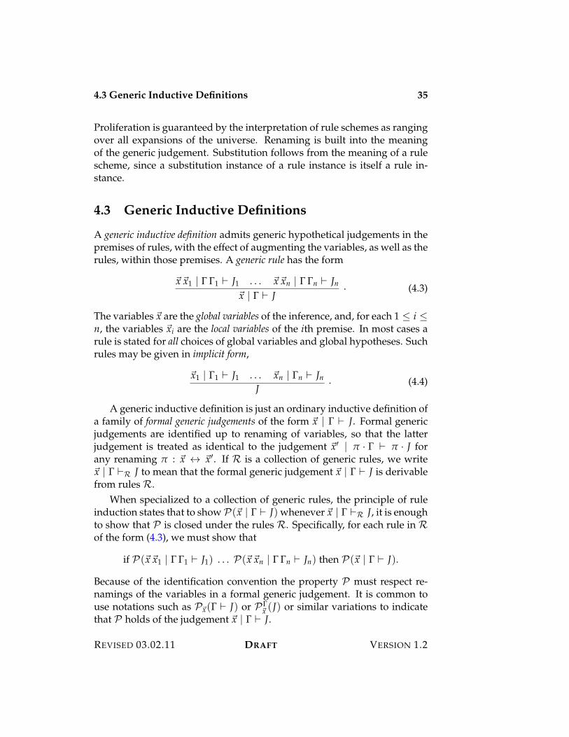
4.3 Generic Inductive Definitions 35
Proliferation is guaranteed by the interpretation of rule schemes as rangingover all expansions of the universe. Renaming is built into the meaningof the generic judgement. Substitution follows from the meaning of a rulescheme, since a substitution instance of a rule instance is itself a rule in-stance.
4.3 Generic Inductive Definitions
A generic inductive definition admits generic hypothetical judgements in thepremises of rules, with the effect of augmenting the variables, as well as therules, within those premises. A generic rule has the form
!x!x1 | ! !1 ) J1 . . . !x!xn | ! !n ) Jn
!x | ! ) J. (4.3)
The variables!x are the global variables of the inference, and, for each 1 ( i (n, the variables !xi are the local variables of the ith premise. In most cases arule is stated for all choices of global variables and global hypotheses. Suchrules may be given in implicit form,
!x1 | !1 ) J1 . . . !xn | !n ) Jn
J. (4.4)
A generic inductive definition is just an ordinary inductive definition ofa family of formal generic judgements of the form !x | ! ) J. Formal genericjudgements are identified up to renaming of variables, so that the latterjudgement is treated as identical to the judgement !x% | # · ! ) # · J forany renaming # : !x . !x%. If R is a collection of generic rules, we write!x | ! )R J to mean that the formal generic judgement !x | ! ) J is derivablefrom rules R.
When specialized to a collection of generic rules, the principle of ruleinduction states that to show P(!x | ! ) J) whenever!x | ! )R J, it is enoughto show that P is closed under the rules R. Specifically, for each rule in Rof the form (4.3), we must show that
if P(!x!x1 | ! !1 ) J1) . . . P(!x!xn | ! !n ) Jn) then P(!x | ! ) J).
Because of the identification convention the property P must respect re-namings of the variables in a formal generic judgement. It is common touse notations such as P!x(! ) J) or P!
!x (J) or similar variations to indicatethat P holds of the judgement !x | ! ) J.
REVISED 03.02.11 DRAFT VERSION 1.2
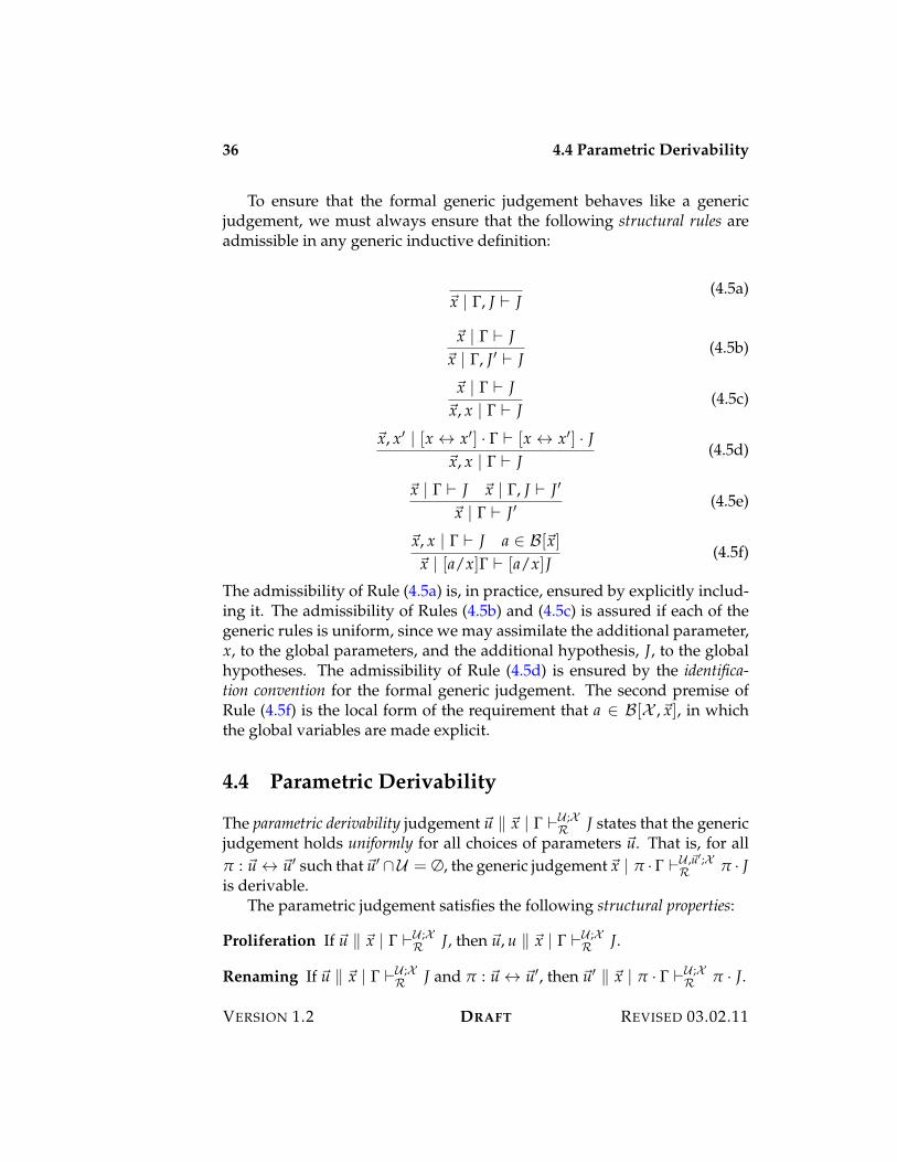
36 4.4 Parametric Derivability
To ensure that the formal generic judgement behaves like a genericjudgement, we must always ensure that the following structural rules areadmissible in any generic inductive definition:
!x | !, J ) J(4.5a)
!x | ! ) J!x | !, J% ) J
(4.5b)
!x | ! ) J!x, x | ! ) J
(4.5c)
!x, x% | [x . x%] · ! ) [x . x%] · J!x, x | ! ) J
(4.5d)
!x | ! ) J !x | !, J ) J%
!x | ! ) J%(4.5e)
!x, x | ! ) J a + B[!x]!x | [a/x]! ) [a/x]J
(4.5f)
The admissibility of Rule (4.5a) is, in practice, ensured by explicitly includ-ing it. The admissibility of Rules (4.5b) and (4.5c) is assured if each of thegeneric rules is uniform, since we may assimilate the additional parameter,x, to the global parameters, and the additional hypothesis, J, to the globalhypotheses. The admissibility of Rule (4.5d) is ensured by the identifica-tion convention for the formal generic judgement. The second premise ofRule (4.5f) is the local form of the requirement that a + B[X ,!x], in whichthe global variables are made explicit.
4.4 Parametric Derivability
The parametric derivability judgement !u / !x | ! )U ;XR J states that the generic
judgement holds uniformly for all choices of parameters !u. That is, for all# : !u . !u% such that!u% 0U = #, the generic judgement!x | # · ! )U ,!u%;X
R # · Jis derivable.
The parametric judgement satisfies the following structural properties:
Proliferation If !u / !x | ! )U ;XR J, then !u, u / !x | ! )U ;X
R J.
Renaming If !u / !x | ! )U ;XR J and # : !u . !u%, then !u% / !x | # · ! )U ;X
R # · J.
VERSION 1.2 DRAFT REVISED 03.02.11
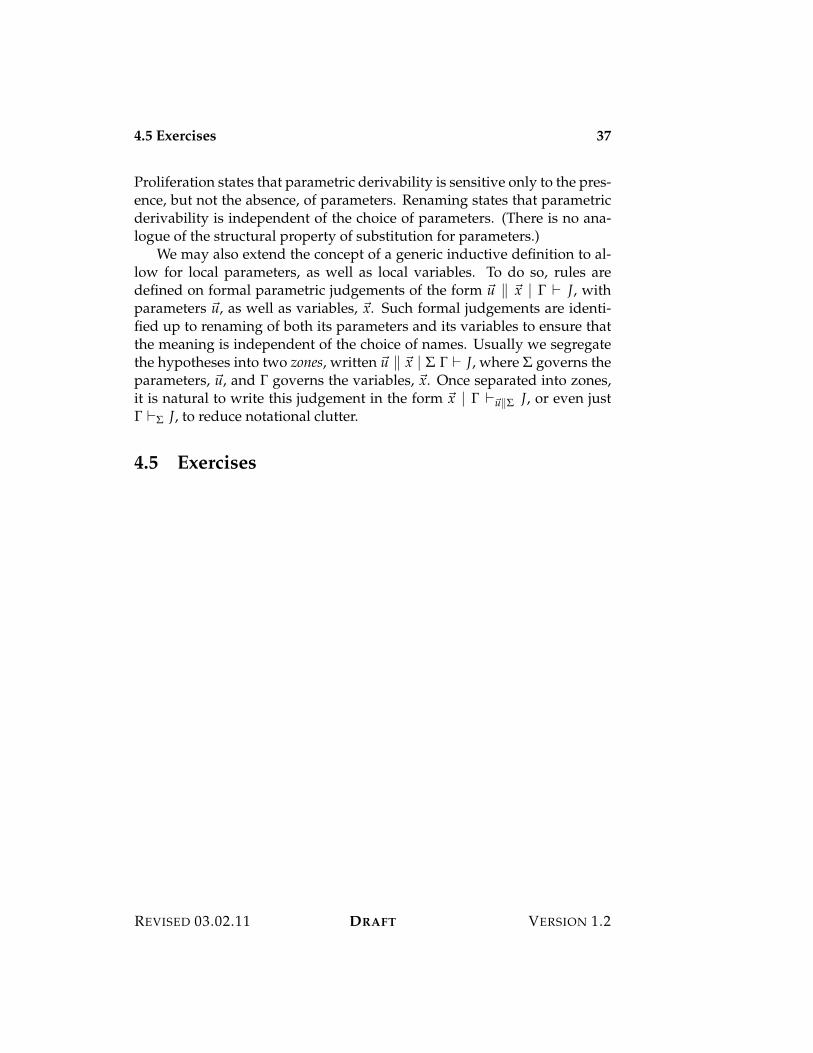
4.5 Exercises 37
Proliferation states that parametric derivability is sensitive only to the pres-ence, but not the absence, of parameters. Renaming states that parametricderivability is independent of the choice of parameters. (There is no ana-logue of the structural property of substitution for parameters.)
We may also extend the concept of a generic inductive definition to al-low for local parameters, as well as local variables. To do so, rules aredefined on formal parametric judgements of the form !u / !x | ! ) J, withparameters !u, as well as variables, !x. Such formal judgements are identi-fied up to renaming of both its parameters and its variables to ensure thatthe meaning is independent of the choice of names. Usually we segregatethe hypotheses into two zones, written !u / !x | $ ! ) J, where $ governs theparameters, !u, and ! governs the variables, !x. Once separated into zones,it is natural to write this judgement in the form !x | ! )!u/$ J, or even just! )$ J, to reduce notational clutter.
4.5 Exercises
REVISED 03.02.11 DRAFT VERSION 1.2

38 4.5 Exercises
VERSION 1.2 DRAFT REVISED 03.02.11

Part II
Levels of Syntax

Chapter 5
Concrete Syntax
The concrete syntax of a language is a means of representing expressions asstrings that may be written on a page or entered using a keyboard. Theconcrete syntax usually is designed to enhance readability and to eliminateambiguity. While there are good methods for eliminating ambiguity, im-proving readability is, to a large extent, a matter of taste.
In this chapter we introduce the main methods for specifying concretesyntax, using as an example an illustrative expression language, calledL{num str}, that supports elementary arithmetic on the natural numbersand simple computations on strings. In addition, L{num str} includes aconstruct for binding the value of an expression to a variable within a spec-ified scope.
5.1 Strings Over An Alphabet
An alphabet is a (finite or infinite) collection of characters. We write c char toindicate that c is a character, and let $ stand for a finite set of such judge-ments, which is sometimes called an alphabet. The judgement $ ) s str,defining the strings over the alphabet $, is inductively defined by the fol-lowing rules:
$ ) % str (5.1a)
$ ) c char $ ) s str$ ) c · s str
(5.1b)
Thus a string is essentially a list of characters, with the null string being theempty list. We often suppress explicit mention of $ when it is clear fromcontext.
42 5.2 Lexical Structure
When specialized to Rules (5.1), the principle of rule induction statesthat to show s P holds whenever s str, it is enough to show
1. % P , and
2. if s P and c char, then c · s P .
This is sometimes called the principle of string induction. It is essentiallyequivalent to induction over the length of a string, except that there is noneed to define the length of a string in order to use it.
The following rules constitute an inductive definition of the judgements1 ˆ s2 = s str, stating that s is the result of concatenating the strings s1 ands2.
% ˆ s = s str (5.2a)s1 ˆ s2 = s str
(c · s1) ˆ s2 = c · s str (5.2b)
It is easy to prove by string induction on the first argument that this judge-ment has mode (&, &, '!). Thus, it determines a total function of its first twoarguments.
String concatenation is associative.
Lemma 5.1. If s1 ˆ s2 = s12 str and s2 ˆ s3 = s23 str, then s1 ˆ s23 = s str ands12 ˆ s3 = s str for some (uniquely determined) string s.
In Section 5.5 on page 48 we will see that this innocuous-seeming factis responsible for most of the complications in defining the concrete syntaxof a language.
Strings are usually written as juxtapositions of characters, writing justabcd for the four-letter string a · (b · (c · (d · %))), for example. Concaten-tation is also written as juxtaposition, and individual characters are oftenidentified with the corresponding unit-length string. This means that abcdcan be thought of in many ways, for example as the concatenations ab cd,a bcd, or abc d, or even % abcd or abcd %, as may be convenient in a givensituation.
5.2 Lexical Structure
The first phase of syntactic processing is to convert from a character-basedrepresentation to a symbol-based representation of the input. This is calledlexical analysis, or lexing. The main idea is to aggregate characters into sym-bols that serve as tokens for subsequent phases of analysis. For example,
VERSION 1.2 DRAFT REVISED 03.02.11
5.2 Lexical Structure 43
the numeral 467 is written as a sequence of three consecutive characters,one for each digit, but is regarded as a single token, namely the number 467.Similarly, an identifier such as temp comprises four letters, but is treated asa single symbol representing the entire word. Moreover, many character-based representations include empty “white space” (spaces, tabs, newlines,and, perhaps, comments) that are discarded by the lexical analyzer.1
The lexical structure of a language is usually described using regular ex-pressions. For example, the lexical structure of L{num str} may be specifiedas follows:
Item itm ::= kwd | id | num | lit | splKeyword kwd ::= l · e · t · % | b · e · % | i · n · %Identifier id ::= ltr (ltr | dig)1Numeral num ::= dig dig1
Literal lit ::= qum (ltr | dig)1qumSpecial spl ::= + | * | ˆ | ( | ) | |Letter ltr ::= a | b | . . .Digit dig ::= 0 | 1 | . . .Quote qum ::= "
A lexical item is either a keyword, an identifier, a numeral, a string literal,or a special symbol. There are three keywords, specified as sequences ofcharacters, for emphasis. Identifiers start with a letter and may involvesubsequent letters or digits. Numerals are non-empty sequences of digits.String literals are sequences of letters or digits surrounded by quotes. Thespecial symbols, letters, digits, and quote marks are as enumerated. (Ob-serve that we tacitly identify a character with the unit-length string consist-ing of that character.)
The job of the lexical analyzer is to translate character strings into tokenstrings using the above definitions as a guide. An input string is scanned,ignoring white space, and translating lexical items into tokens, which arespecified by the following rules:
s strID[s] tok
(5.3a)
n natNUM[n] tok
(5.3b)
s strLIT[s] tok
(5.3c)
1In some languages white space is significant, in which case it must be converted tosymbolic form for subsequent processing.
REVISED 03.02.11 DRAFT VERSION 1.2
44 5.2 Lexical Structure
LET tok (5.3d)
BE tok (5.3e)
IN tok (5.3f)
ADD tok (5.3g)
MUL tok (5.3h)
CAT tok (5.3i)
LP tok (5.3j)
RP tok (5.3k)
VB tok (5.3l)
Rule (5.3a) admits any string as an identifier, even though only certainstrings will be treated as identifiers by the lexical analyzer.
Lexical analysis is inductively defined by the following judgement forms:
s charstr 23 t tokstr Scan inputs itm 23 t tok Scan an item
s kwd 23 t tok Scan a keywords id 23 t tok Scan an identifier
s num 23 t tok Scan a numbers spl 23 t tok Scan a symbols lit 23 t tok Scan a string literal
The definition of these forms, which follows, makes use of several auxiliaryjudgements corresponding to the classifications of characters in the lexicalstructure of the language. For example, s whs states that the string s consistsonly of “white space”, s lord states that s is either an alphabetic letter or adigit, and s non-lord states that s does not begin with a letter or digit, andso forth.
% charstr 23 % tokstr (5.4a)
s = s1 ˆ s2 ˆ s3 str s1 whs s2 itm 23 t tok s3 charstr 23 ts tokstrs charstr 23 t · ts tokstr
(5.4b)s kwd 23 t toks itm 23 t tok (5.4c)
s id 23 t toks itm 23 t tok (5.4d)
VERSION 1.2 DRAFT REVISED 03.02.11
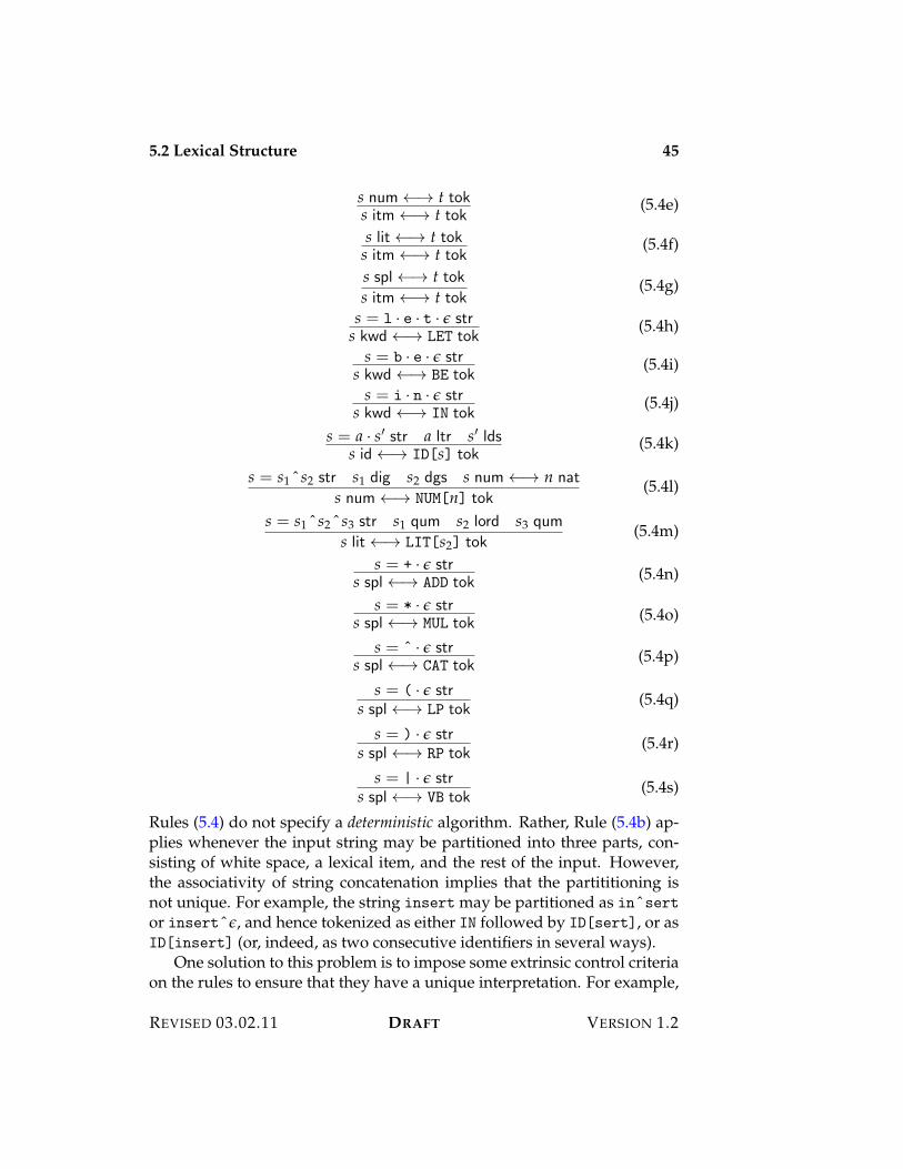
5.2 Lexical Structure 45
s num 23 t toks itm 23 t tok (5.4e)
s lit 23 t toks itm 23 t tok (5.4f)
s spl 23 t toks itm 23 t tok
(5.4g)
s = l · e · t · % strs kwd 23 LET tok
(5.4h)
s = b · e · % strs kwd 23 BE tok
(5.4i)
s = i · n · % strs kwd 23 IN tok
(5.4j)
s = a · s% str a ltr s% ldss id 23 ID[s] tok
(5.4k)
s = s1 ˆ s2 str s1 dig s2 dgs s num 23 n nats num 23 NUM[n] tok
(5.4l)
s = s1 ˆ s2 ˆ s3 str s1 qum s2 lord s3 qums lit 23 LIT[s2] tok
(5.4m)
s = + · % strs spl 23 ADD tok (5.4n)
s = * · % strs spl 23 MUL tok (5.4o)
s = ˆ · % strs spl 23 CAT tok
(5.4p)
s = ( · % strs spl 23 LP tok
(5.4q)
s = ) · % strs spl 23 RP tok
(5.4r)
s = | · % strs spl 23 VB tok
(5.4s)
Rules (5.4) do not specify a deterministic algorithm. Rather, Rule (5.4b) ap-plies whenever the input string may be partitioned into three parts, con-sisting of white space, a lexical item, and the rest of the input. However,the associativity of string concatenation implies that the partititioning isnot unique. For example, the string insert may be partitioned as in ˆsertor insert ˆ %, and hence tokenized as either IN followed by ID[sert], or asID[insert] (or, indeed, as two consecutive identifiers in several ways).
One solution to this problem is to impose some extrinsic control criteriaon the rules to ensure that they have a unique interpretation. For example,
REVISED 03.02.11 DRAFT VERSION 1.2
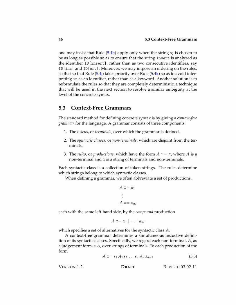
46 5.3 Context-Free Grammars
one may insist that Rule (5.4b) apply only when the string s2 is chosen tobe as long as possible so as to ensure that the string insert is analyzed asthe identifier ID[insert], rather than as two consecutive identifiers, sayID[ins] and ID[ert]. Moreover, we may impose an ordering on the rules,so that so that Rule (5.4j) takes priority over Rule (5.4k) so as to avoid inter-preting in as an identifier, rather than as a keyword. Another solution is toreformulate the rules so that they are completely deterministic, a techniquethat will be used in the next section to resolve a similar ambiguity at thelevel of the concrete syntax.
5.3 Context-Free Grammars
The standard method for defining concrete syntax is by giving a context-freegrammar for the language. A grammar consists of three components:
1. The tokens, or terminals, over which the grammar is defined.
2. The syntactic classes, or non-terminals, which are disjoint from the ter-minals.
3. The rules, or productions, which have the form A ::= $, where A is anon-terminal and $ is a string of terminals and non-terminals.
Each syntactic class is a collection of token strings. The rules determinewhich strings belong to which syntactic classes.
When defining a grammar, we often abbreviate a set of productions,
A ::= $1
...A ::= $n,
each with the same left-hand side, by the compound production
A ::= $1 | . . . | $n,
which specifies a set of alternatives for the syntactic class A.A context-free grammar determines a simultaneous inductive defini-
tion of its syntactic classes. Specifically, we regard each non-terminal, A, asa judgement form, s A, over strings of terminals. To each production of theform
A ::= s1 A1 s2 . . . sn An sn+1 (5.5)
VERSION 1.2 DRAFT REVISED 03.02.11
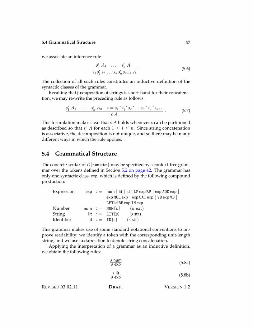
5.4 Grammatical Structure 47
we associate an inference rule
s%1 A1 . . . s%n An
s1 s%1 s2 . . . sn s%n sn+1 A. (5.6)
The collection of all such rules constitutes an inductive definition of thesyntactic classes of the grammar.
Recalling that juxtaposition of strings is short-hand for their concatena-tion, we may re-write the preceding rule as follows:
s%1 A1 . . . s%n An s = s1 ˆ s%1 ˆ s2 ˆ . . . sn ˆ s%n ˆ sn+1
s A. (5.7)
This formulation makes clear that s A holds whenever s can be partitionedas described so that s%i A for each 1 ( i ( n. Since string concatenationis associative, the decomposition is not unique, and so there may be manydifferent ways in which the rule applies.
5.4 Grammatical Structure
The concrete syntax of L{num str} may be specified by a context-free gram-mar over the tokens defined in Section 5.2 on page 42. The grammar hasonly one syntactic class, exp, which is defined by the following compoundproduction:
Expression exp ::= num | lit | id | LP exp RP | exp ADD exp |exp MUL exp | exp CAT exp | VB exp VB |LET id BE exp IN exp
Number num ::= NUM[n] (n nat)String lit ::= LIT[s] (s str)Identifier id ::= ID[s] (s str)
This grammar makes use of some standard notational conventions to im-prove readability: we identify a token with the corresponding unit-lengthstring, and we use juxtaposition to denote string concatenation.
Applying the interpretation of a grammar as an inductive definition,we obtain the following rules:
s nums exp (5.8a)
s lits exp (5.8b)
REVISED 03.02.11 DRAFT VERSION 1.2
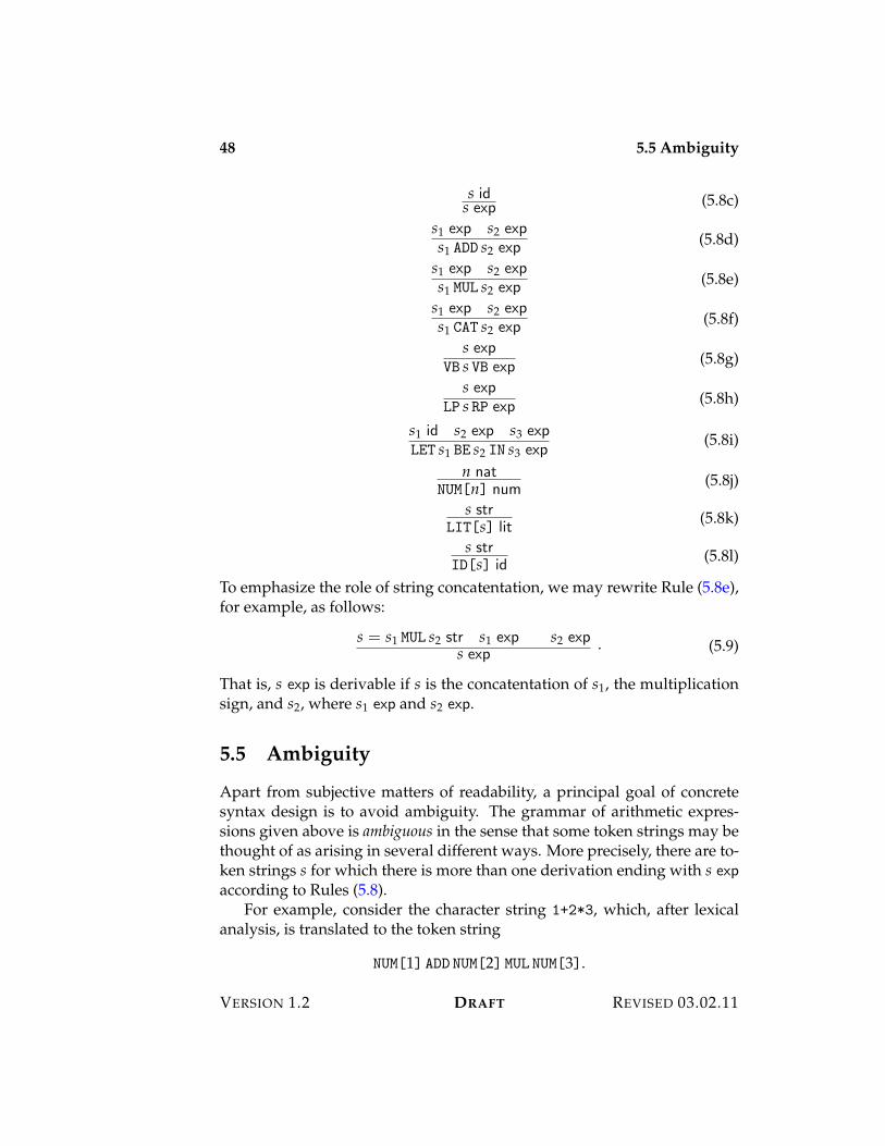
48 5.5 Ambiguity
s ids exp (5.8c)
s1 exp s2 exps1 ADD s2 exp (5.8d)
s1 exp s2 exps1 MUL s2 exp (5.8e)
s1 exp s2 exps1 CAT s2 exp (5.8f)
s expVB s VB exp (5.8g)
s expLP s RP exp (5.8h)
s1 id s2 exp s3 expLET s1 BE s2 IN s3 exp
(5.8i)
n natNUM[n] num
(5.8j)
s strLIT[s] lit
(5.8k)
s strID[s] id
(5.8l)
To emphasize the role of string concatentation, we may rewrite Rule (5.8e),for example, as follows:
s = s1 MUL s2 str s1 exp s2 exps exp . (5.9)
That is, s exp is derivable if s is the concatentation of s1, the multiplicationsign, and s2, where s1 exp and s2 exp.
5.5 Ambiguity
Apart from subjective matters of readability, a principal goal of concretesyntax design is to avoid ambiguity. The grammar of arithmetic expres-sions given above is ambiguous in the sense that some token strings may bethought of as arising in several different ways. More precisely, there are to-ken strings s for which there is more than one derivation ending with s expaccording to Rules (5.8).
For example, consider the character string 1+2*3, which, after lexicalanalysis, is translated to the token string
NUM[1] ADD NUM[2] MUL NUM[3].
VERSION 1.2 DRAFT REVISED 03.02.11
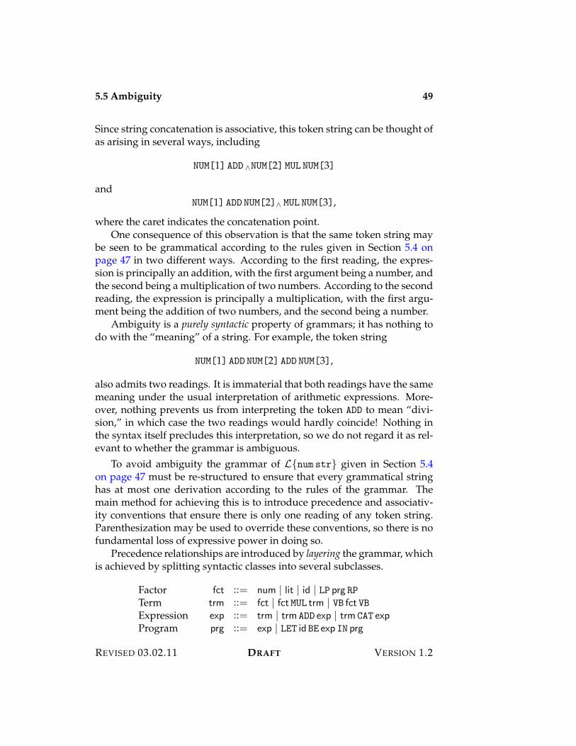
5.5 Ambiguity 49
Since string concatenation is associative, this token string can be thought ofas arising in several ways, including
NUM[1] ADD 4NUM[2] MUL NUM[3]
andNUM[1] ADD NUM[2]4 MUL NUM[3],
where the caret indicates the concatenation point.One consequence of this observation is that the same token string may
be seen to be grammatical according to the rules given in Section 5.4 onpage 47 in two different ways. According to the first reading, the expres-sion is principally an addition, with the first argument being a number, andthe second being a multiplication of two numbers. According to the secondreading, the expression is principally a multiplication, with the first argu-ment being the addition of two numbers, and the second being a number.
Ambiguity is a purely syntactic property of grammars; it has nothing todo with the “meaning” of a string. For example, the token string
NUM[1] ADD NUM[2] ADD NUM[3],
also admits two readings. It is immaterial that both readings have the samemeaning under the usual interpretation of arithmetic expressions. More-over, nothing prevents us from interpreting the token ADD to mean “divi-sion,” in which case the two readings would hardly coincide! Nothing inthe syntax itself precludes this interpretation, so we do not regard it as rel-evant to whether the grammar is ambiguous.
To avoid ambiguity the grammar of L{num str} given in Section 5.4on page 47 must be re-structured to ensure that every grammatical stringhas at most one derivation according to the rules of the grammar. Themain method for achieving this is to introduce precedence and associativ-ity conventions that ensure there is only one reading of any token string.Parenthesization may be used to override these conventions, so there is nofundamental loss of expressive power in doing so.
Precedence relationships are introduced by layering the grammar, whichis achieved by splitting syntactic classes into several subclasses.
Factor fct ::= num | lit | id | LP prg RPTerm trm ::= fct | fct MUL trm | VB fct VBExpression exp ::= trm | trm ADD exp | trm CAT expProgram prg ::= exp | LET id BE exp IN prg
REVISED 03.02.11 DRAFT VERSION 1.2
50 5.6 Exercises
The effect of this grammar is to ensure that let has the lowest precedence,addition and concatenation intermediate precedence, and multiplicationand length the highest precedence. Moreover, all forms are right-associative.Other choices of rules are possible, according to taste; this grammar illus-trates one way to resolve the ambiguities of the original expression gram-mar.
5.6 Exercises
VERSION 1.2 DRAFT REVISED 03.02.11
Chapter 6
Abstract Syntax
The concrete syntax of a language is concerned with the linear representa-tion of the phrases of a language as strings of symbols—the form in whichwe write them on paper, type them into a computer, and read them froma page. But languages are also the subjects of study, as well as the instru-ments of expression. As such the concrete syntax of a language is just a nui-sance. When analyzing a language mathematically we are only interestedin the deep structure of its phrases, not their surface representation. The ab-stract syntax of a language exposes the hierarchical and binding structureof the language. Parsing is the process of translation from concrete to ab-stract syntax. It consists of analyzing the linear representation of a phrasein terms of the grammar of the language and transforming it into an ab-stract syntax tree or an abstract binding tree that reveals the deep structureof the phrase. Formatting is the inverse process of generating a linear repre-sentation of a given piece of abstract syntax.
6.1 Hierarchical and Binding Structure
For the purposes of analysis the most important elements of the syntax ofa language are its hierarchical and binding structure. Ignoring binding andscope, the hierarchical structure of a language may be expressed using ab-stract syntax trees. Accounting for these requires the additional structureof abstract binding trees. We will define both an ast and an abt representa-tion of L{num str} in order to compare the two and show how they relateto the concrete syntax described in Chapter 5.
The purely hierarchical abstract syntax of L{num str} is generated by
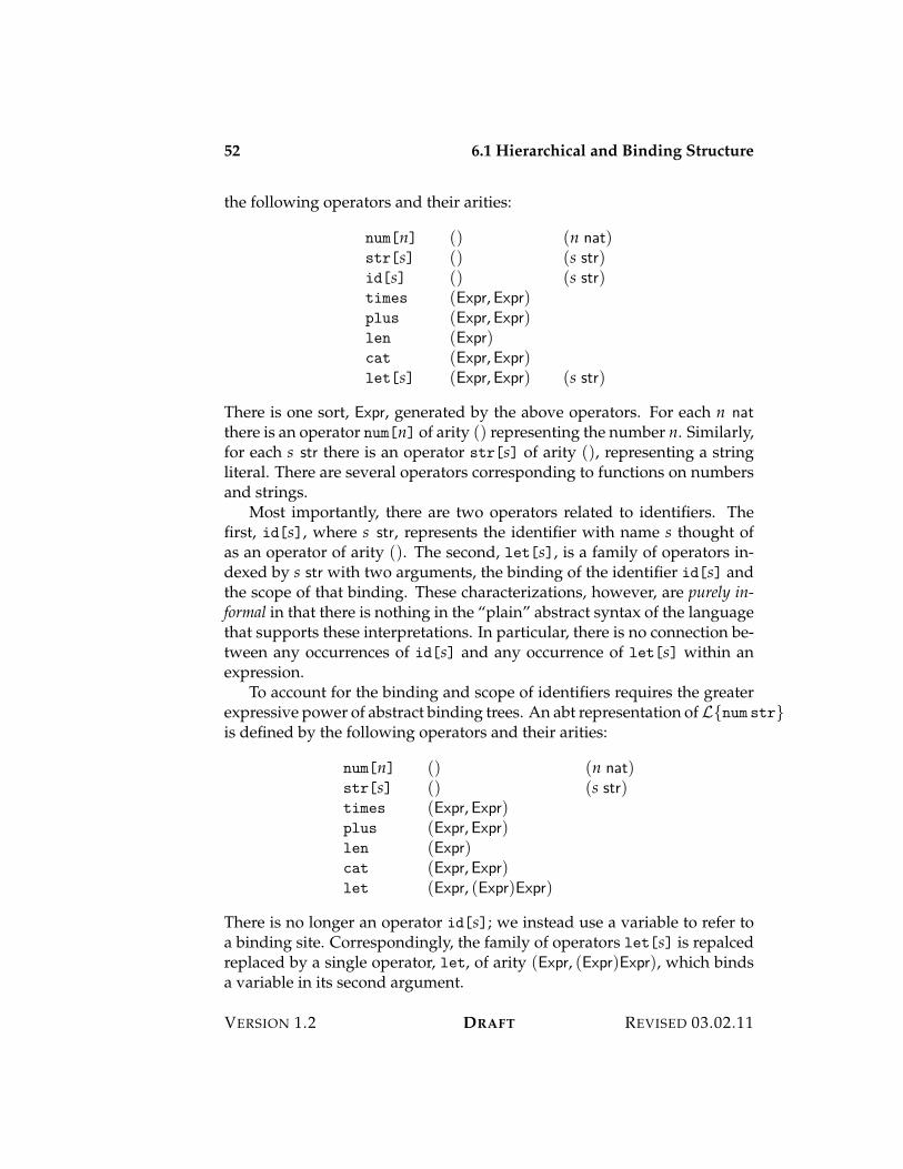
52 6.1 Hierarchical and Binding Structure
the following operators and their arities:
num[n] () (n nat)str[s] () (s str)id[s] () (s str)times (Expr,Expr)plus (Expr,Expr)len (Expr)cat (Expr,Expr)let[s] (Expr,Expr) (s str)
There is one sort, Expr, generated by the above operators. For each n natthere is an operator num[n] of arity () representing the number n. Similarly,for each s str there is an operator str[s] of arity (), representing a stringliteral. There are several operators corresponding to functions on numbersand strings.
Most importantly, there are two operators related to identifiers. Thefirst, id[s], where s str, represents the identifier with name s thought ofas an operator of arity (). The second, let[s], is a family of operators in-dexed by s str with two arguments, the binding of the identifier id[s] andthe scope of that binding. These characterizations, however, are purely in-formal in that there is nothing in the “plain” abstract syntax of the languagethat supports these interpretations. In particular, there is no connection be-tween any occurrences of id[s] and any occurrence of let[s] within anexpression.
To account for the binding and scope of identifiers requires the greaterexpressive power of abstract binding trees. An abt representation of L{num str}is defined by the following operators and their arities:
num[n] () (n nat)str[s] () (s str)times (Expr,Expr)plus (Expr,Expr)len (Expr)cat (Expr,Expr)let (Expr, (Expr)Expr)
There is no longer an operator id[s]; we instead use a variable to refer toa binding site. Correspondingly, the family of operators let[s] is repalcedreplaced by a single operator, let, of arity (Expr, (Expr)Expr), which bindsa variable in its second argument.
VERSION 1.2 DRAFT REVISED 03.02.11
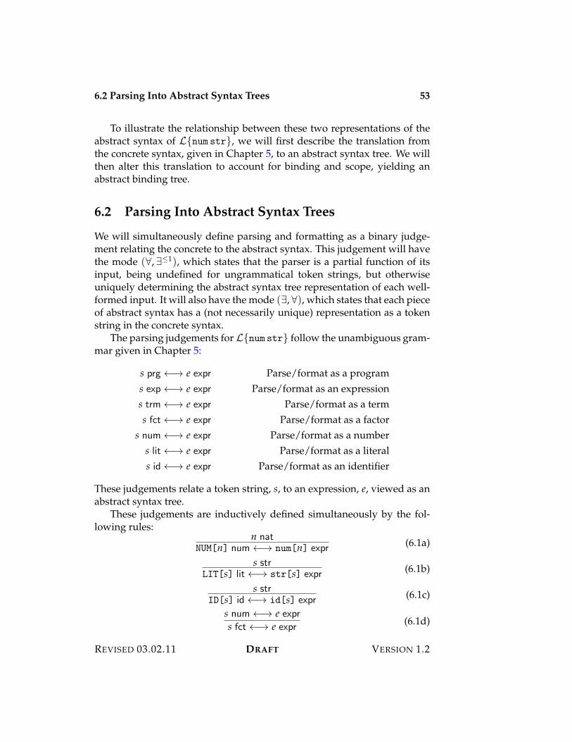
6.2 Parsing Into Abstract Syntax Trees 53
To illustrate the relationship between these two representations of theabstract syntax of L{num str}, we will first describe the translation fromthe concrete syntax, given in Chapter 5, to an abstract syntax tree. We willthen alter this translation to account for binding and scope, yielding anabstract binding tree.
6.2 Parsing Into Abstract Syntax Trees
We will simultaneously define parsing and formatting as a binary judge-ment relating the concrete to the abstract syntax. This judgement will havethe mode (&, '(1), which states that the parser is a partial function of itsinput, being undefined for ungrammatical token strings, but otherwiseuniquely determining the abstract syntax tree representation of each well-formed input. It will also have the mode (', &), which states that each pieceof abstract syntax has a (not necessarily unique) representation as a tokenstring in the concrete syntax.
The parsing judgements for L{num str} follow the unambiguous gram-mar given in Chapter 5:
s prg 23 e expr Parse/format as a programs exp 23 e expr Parse/format as an expressions trm 23 e expr Parse/format as a terms fct 23 e expr Parse/format as a factor
s num 23 e expr Parse/format as a numbers lit 23 e expr Parse/format as a literals id 23 e expr Parse/format as an identifier
These judgements relate a token string, s, to an expression, e, viewed as anabstract syntax tree.
These judgements are inductively defined simultaneously by the fol-lowing rules:
n natNUM[n] num 23 num[n] expr (6.1a)
s strLIT[s] lit 23 str[s] expr (6.1b)
s strID[s] id 23 id[s] expr (6.1c)
s num 23 e exprs fct 23 e expr (6.1d)
REVISED 03.02.11 DRAFT VERSION 1.2
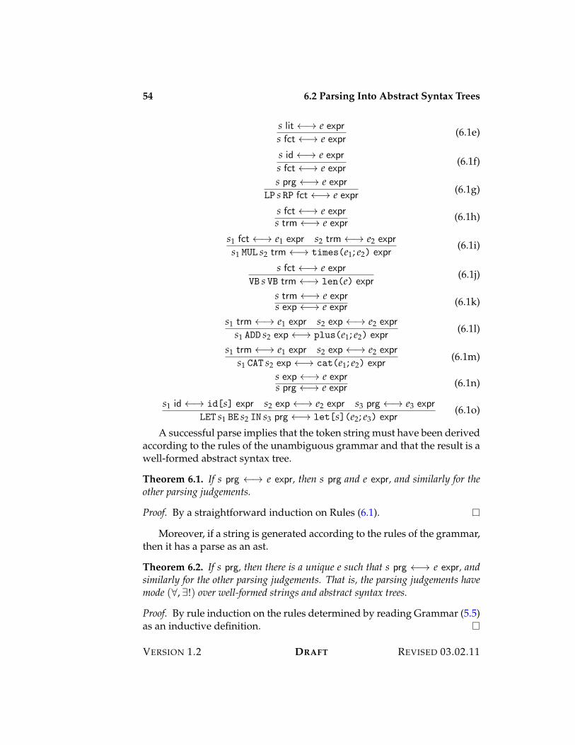
54 6.2 Parsing Into Abstract Syntax Trees
s lit 23 e exprs fct 23 e expr (6.1e)
s id 23 e exprs fct 23 e expr (6.1f)
s prg 23 e exprLP s RP fct 23 e expr (6.1g)
s fct 23 e exprs trm 23 e expr (6.1h)
s1 fct 23 e1 expr s2 trm 23 e2 exprs1 MUL s2 trm 23 times(e1; e2) expr
(6.1i)
s fct 23 e exprVB s VB trm 23 len(e) expr
(6.1j)
s trm 23 e exprs exp 23 e expr (6.1k)
s1 trm 23 e1 expr s2 exp 23 e2 exprs1 ADD s2 exp 23 plus(e1; e2) expr
(6.1l)
s1 trm 23 e1 expr s2 exp 23 e2 exprs1 CAT s2 exp 23 cat(e1; e2) expr
(6.1m)
s exp 23 e exprs prg 23 e expr (6.1n)
s1 id 23 id[s] expr s2 exp 23 e2 expr s3 prg 23 e3 exprLET s1 BE s2 IN s3 prg 23 let[s](e2; e3) expr
(6.1o)
A successful parse implies that the token string must have been derivedaccording to the rules of the unambiguous grammar and that the result is awell-formed abstract syntax tree.
Theorem 6.1. If s prg 23 e expr, then s prg and e expr, and similarly for theother parsing judgements.
Proof. By a straightforward induction on Rules (6.1).
Moreover, if a string is generated according to the rules of the grammar,then it has a parse as an ast.
Theorem 6.2. If s prg, then there is a unique e such that s prg 23 e expr, andsimilarly for the other parsing judgements. That is, the parsing judgements havemode (&, '!) over well-formed strings and abstract syntax trees.
Proof. By rule induction on the rules determined by reading Grammar (5.5)as an inductive definition.
VERSION 1.2 DRAFT REVISED 03.02.11
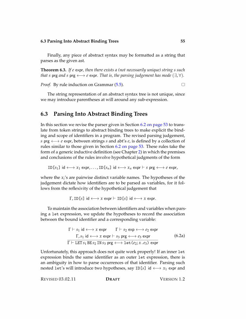
6.3 Parsing Into Abstract Binding Trees 55
Finally, any piece of abstract syntax may be formatted as a string thatparses as the given ast.
Theorem 6.3. If e expr, then there exists a (not necessarily unique) string s suchthat s prg and s prg 23 e expr. That is, the parsing judgement has mode (', &).
Proof. By rule induction on Grammar (5.5).
The string representation of an abstract syntax tree is not unique, sincewe may introduce parentheses at will around any sub-expression.
6.3 Parsing Into Abstract Binding Trees
In this section we revise the parser given in Section 6.2 on page 53 to trans-late from token strings to abstract binding trees to make explicit the bind-ing and scope of identifiers in a program. The revised parsing judgement,s prg 23 e expr, between strings s and abt’s e, is defined by a collection ofrules similar to those given in Section 6.2 on page 53. These rules take theform of a generic inductive definition (see Chapter 2) in which the premisesand conclusions of the rules involve hypothetical judgments of the form
ID[s1] id 23 x1 expr, . . . , ID[sn] id 23 xn expr ) s prg 23 e expr,
where the xi’s are pairwise distinct variable names. The hypotheses of thejudgement dictate how identifiers are to be parsed as variables, for it fol-lows from the reflexivity of the hypothetical judgement that
!, ID[s] id 23 x expr ) ID[s] id 23 x expr.
To maintain the association between identifiers and variables when pars-ing a let expression, we update the hypotheses to record the associationbetween the bound identifier and a corresponding variable:
! ) s1 id 23 x expr ! ) s2 exp 23 e2 expr
!, s1 id 23 x expr ) s3 prg 23 e3 expr
! ) LET s1 BE s2 IN s3 prg 23 let(e2; x.e3) expr
(6.2a)
Unfortunately, this approach does not quite work properly! If an inner letexpression binds the same identifier as an outer let expression, there isan ambiguity in how to parse occurrences of that identifier. Parsing suchnested let’s will introduce two hypotheses, say ID[s] id 23 x1 expr and
REVISED 03.02.11 DRAFT VERSION 1.2
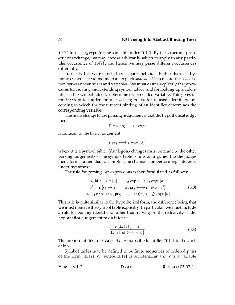
56 6.3 Parsing Into Abstract Binding Trees
ID[s] id 23 x2 expr, for the same identifier ID[s]. By the structural prop-erty of exchange, we may choose arbitrarily which to apply to any partic-ular occurrence of ID[s], and hence we may parse different occurrencesdifferently.
To rectify this we resort to less elegant methods. Rather than use hy-potheses, we instead maintain an explicit symbol table to record the associa-tion between identifiers and variables. We must define explicitly the proce-dures for creating and extending symbol tables, and for looking up an iden-tifier in the symbol table to determine its associated variable. This gives usthe freedom to implement a shadowing policy for re-used identifiers, ac-cording to which the most recent binding of an identifier determines thecorresponding variable.
The main change to the parsing judgement is that the hypothetical judge-ment
! ) s prg 23 e expr
is reduced to the basic judgement
s prg 23 e expr [&],
where & is a symbol table. (Analogous changes must be made to the otherparsing judgements.) The symbol table is now an argument to the judge-ment form, rather than an implicit mechanism for performing inferenceunder hypotheses.
The rule for parsing let expressions is then formulated as follows:
s1 id 23 x [&] s2 exp 23 e2 expr [&]
&% = &[s1 53 x] s3 prg 23 e3 expr [&%]
LET s1 BE s2 IN s3 prg 23 let(e2; x.e3) expr [&]
(6.3)
This rule is quite similar to the hypothetical form, the difference being thatwe must manage the symbol table explicitly. In particular, we must includea rule for parsing identifiers, rather than relying on the reflexivity of thehypothetical judgement to do it for us.
&(ID[s]) = xID[s] id 23 x [&]
(6.4)
The premise of this rule states that & maps the identifier ID[s] to the vari-able x.
Symbol tables may be defined to be finite sequences of ordered pairsof the form (ID[s], x), where ID[s] is an identifier and x is a variable
VERSION 1.2 DRAFT REVISED 03.02.11
6.4 Exercises 57
name. Using this representation it is straightforward to define the follow-ing judgement forms:
& symtab well-formed symbol table&% = &[ID[s] 53 x] add new association
&(ID[s]) = x lookup identifier
We leave the precise definitions of these judgements as an exercise for thereader.
6.4 Exercises
REVISED 03.02.11 DRAFT VERSION 1.2

58 6.4 Exercises
VERSION 1.2 DRAFT REVISED 03.02.11
Part III
Statics and Dynamics

Chapter 7
Statics
Most programming languages exhibit a phase distinction between the staticand dynamic phases of processing. The static phase consists of parsingand type checking to ensure that the program is well-formed; the dynamicphase consists of execution of well-formed programs. A language is saidto be safe exactly when well-formed programs are well-behaved when exe-cuted.
The static phase is specified by a statics comprising a collection of rulesfor deriving typing judgements stating that an expression is well-formed ofa certain type. Types mediate the interaction between the constituent partsof a program by “predicting” some aspects of the execution behavior of theparts so that we may ensure they fit together properly at run-time. Typesafety tells us that these predictions are accurate; if not, the statics is con-sidered to be improperly defined, and the language is deemed unsafe forexecution.
In this chapter we present the statics of the language L{num str} as anillustration of the methodology that we shall employ throughout this book.
7.1 Syntax
When defining a language we shall be primarily concerned with its abstractsyntax, specified by a collection of operators and their arities. The abstractsyntax provides a systematic, unambiguous account of the hierarchical andbinding structure of the language, and is therefore to be considered theofficial presentation of the language. However, for the sake perspicuity ofexamples, it is also useful to specify minimal concrete syntax conventions,without going through the trouble to set up a fully precise grammar for it.
62 7.2 Type System
We will accomplish both of these purposes with a syntax chart, whosemeaning is best illustrated by example. The following chart summarizesthe abstract and concrete syntax of L{num str}, which was analyzed in de-tail in Chapters 5 and 6.
Type " ::= num num numbersstr str strings
Expr e ::= x x variablenum[n] n numeralstr[s] ”s” literalplus(e1; e2) e1 + e2 additiontimes(e1; e2) e1 1 e2 multiplicationcat(e1; e2) e1 ^ e2 concatenationlen(e) |e| lengthlet(e1; x.e2) let x be e1 in e2 definition
There are two sorts, Type ranged over by the meta-variable ", and Expr,ranged over by the meta-variable e. The meta-variable x ranges over vari-ables of sort Expr. The chart defines a number of operators and their arities.For example, the operator let has arity (Expr, (Expr)Expr), which specifiesthat it has two arguments of sort Expr, and binds a variable of sort Expr inthe second argument.
7.2 Type System
The role of a type system is to impose constraints on the formations ofphrases that are sensitive to the context in which they occur. For exam-ple, whether or not the expression plus(x; num[n]) is sensible depends onwhether or not the variable x is declared to have type num in the surround-ing context of the expression. This example is, in fact, illustrative of thegeneral case, in that the only information required about the context of anexpression is the type of the variables within whose scope the expressionlies. Consequently, the statics of L{num str} consists of an inductive defi-nition of generic hypothetical judgements of the form
!x | ! ) e : ",
where !x is a finite set of variables, and ! is a typing context consisting ofhypotheses of the form x : ", one for each x + X . We rely on typographicalconventions to determine the set of variables, using the letters x and y for
VERSION 1.2 DRAFT REVISED 03.02.11
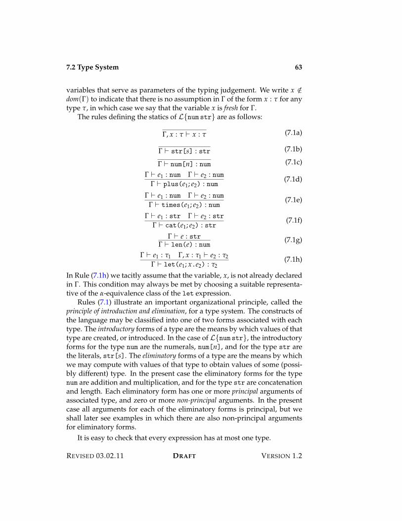
7.2 Type System 63
variables that serve as parameters of the typing judgement. We write x /+dom(!) to indicate that there is no assumption in ! of the form x : " for anytype ", in which case we say that the variable x is fresh for !.
The rules defining the statics of L{num str} are as follows:
!, x : " ) x : " (7.1a)
! ) str[s] : str (7.1b)
! ) num[n] : num (7.1c)
! ) e1 : num ! ) e2 : num! ) plus(e1; e2) : num
(7.1d)
! ) e1 : num ! ) e2 : num! ) times(e1; e2) : num
(7.1e)
! ) e1 : str ! ) e2 : str! ) cat(e1; e2) : str
(7.1f)
! ) e : str! ) len(e) : num (7.1g)
! ) e1 : "1 !, x : "1 ) e2 : "2! ) let(e1; x.e2) : "2
(7.1h)
In Rule (7.1h) we tacitly assume that the variable, x, is not already declaredin !. This condition may always be met by choosing a suitable representa-tive of the $-equivalence class of the let expression.
Rules (7.1) illustrate an important organizational principle, called theprinciple of introduction and elimination, for a type system. The constructs ofthe language may be classified into one of two forms associated with eachtype. The introductory forms of a type are the means by which values of thattype are created, or introduced. In the case of L{num str}, the introductoryforms for the type num are the numerals, num[n], and for the type str arethe literals, str[s]. The eliminatory forms of a type are the means by whichwe may compute with values of that type to obtain values of some (possi-bly different) type. In the present case the eliminatory forms for the typenum are addition and multiplication, and for the type str are concatenationand length. Each eliminatory form has one or more principal arguments ofassociated type, and zero or more non-principal arguments. In the presentcase all arguments for each of the eliminatory forms is principal, but weshall later see examples in which there are also non-principal argumentsfor eliminatory forms.
It is easy to check that every expression has at most one type.
REVISED 03.02.11 DRAFT VERSION 1.2
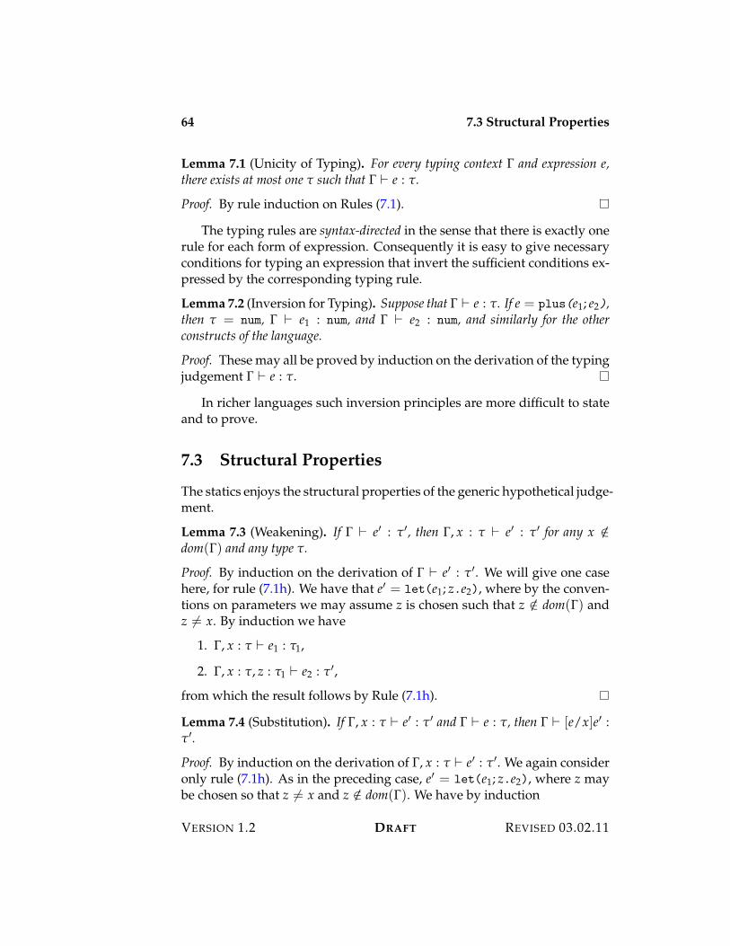
64 7.3 Structural Properties
Lemma 7.1 (Unicity of Typing). For every typing context ! and expression e,there exists at most one " such that ! ) e : ".
Proof. By rule induction on Rules (7.1).
The typing rules are syntax-directed in the sense that there is exactly onerule for each form of expression. Consequently it is easy to give necessaryconditions for typing an expression that invert the sufficient conditions ex-pressed by the corresponding typing rule.
Lemma 7.2 (Inversion for Typing). Suppose that ! ) e : ". If e = plus(e1; e2),then " = num, ! ) e1 : num, and ! ) e2 : num, and similarly for the otherconstructs of the language.
Proof. These may all be proved by induction on the derivation of the typingjudgement ! ) e : ".
In richer languages such inversion principles are more difficult to stateand to prove.
7.3 Structural Properties
The statics enjoys the structural properties of the generic hypothetical judge-ment.
Lemma 7.3 (Weakening). If ! ) e% : "%, then !, x : " ) e% : "% for any x /+dom(!) and any type ".
Proof. By induction on the derivation of ! ) e% : "%. We will give one casehere, for rule (7.1h). We have that e% = let(e1; z.e2), where by the conven-tions on parameters we may assume z is chosen such that z /+ dom(!) andz ,= x. By induction we have
1. !, x : " ) e1 : "1,
2. !, x : ", z : "1 ) e2 : "%,
from which the result follows by Rule (7.1h).
Lemma 7.4 (Substitution). If !, x : " ) e% : "% and ! ) e : ", then ! ) [e/x]e% :"%.
Proof. By induction on the derivation of !, x : " ) e% : "%. We again consideronly rule (7.1h). As in the preceding case, e% = let(e1; z.e2), where z maybe chosen so that z ,= x and z /+ dom(!). We have by induction
VERSION 1.2 DRAFT REVISED 03.02.11
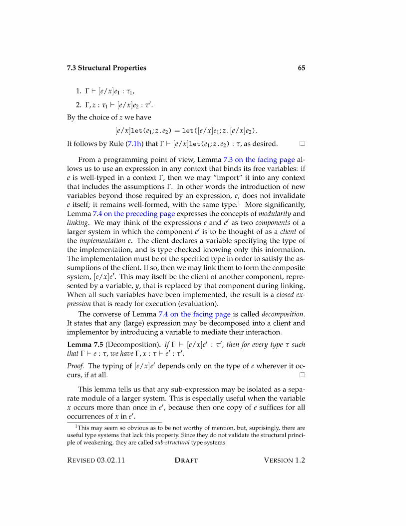
7.3 Structural Properties 65
1. ! ) [e/x]e1 : "1,
2. !, z : "1 ) [e/x]e2 : "%.
By the choice of z we have
[e/x]let(e1; z.e2) = let([e/x]e1; z.[e/x]e2).
It follows by Rule (7.1h) that ! ) [e/x]let(e1; z.e2) : ", as desired.
From a programming point of view, Lemma 7.3 on the facing page al-lows us to use an expression in any context that binds its free variables: ife is well-typed in a context !, then we may “import” it into any contextthat includes the assumptions !. In other words the introduction of newvariables beyond those required by an expression, e, does not invalidatee itself; it remains well-formed, with the same type.1 More significantly,Lemma 7.4 on the preceding page expresses the concepts of modularity andlinking. We may think of the expressions e and e% as two components of alarger system in which the component e% is to be thought of as a client ofthe implementation e. The client declares a variable specifying the type ofthe implementation, and is type checked knowing only this information.The implementation must be of the specified type in order to satisfy the as-sumptions of the client. If so, then we may link them to form the compositesystem, [e/x]e%. This may itself be the client of another component, repre-sented by a variable, y, that is replaced by that component during linking.When all such variables have been implemented, the result is a closed ex-pression that is ready for execution (evaluation).
The converse of Lemma 7.4 on the facing page is called decomposition.It states that any (large) expression may be decomposed into a client andimplementor by introducing a variable to mediate their interaction.
Lemma 7.5 (Decomposition). If ! ) [e/x]e% : "%, then for every type " suchthat ! ) e : ", we have !, x : " ) e% : "%.
Proof. The typing of [e/x]e% depends only on the type of e wherever it oc-curs, if at all.
This lemma tells us that any sub-expression may be isolated as a sepa-rate module of a larger system. This is especially useful when the variablex occurs more than once in e%, because then one copy of e suffices for alloccurrences of x in e%.
1This may seem so obvious as to be not worthy of mention, but, suprisingly, there areuseful type systems that lack this property. Since they do not validate the structural princi-ple of weakening, they are called sub-structural type systems.
REVISED 03.02.11 DRAFT VERSION 1.2
66 7.4 Exercises
7.4 Exercises
1. Show that the expression e = plus(num[7]; str[abc]) is ill-typed inthat there is no " such that e : ".
VERSION 1.2 DRAFT REVISED 03.02.11
Chapter 8
Dynamics
The dynamics of a language is a description of how programs are to be ex-ecuted. The most important way to define the dynamics of a language isby the method of structural dynamics, which defines a transition system thatinductively specifies the step-by-step process of executing a program. An-other method for presenting dynamics, called contextual dynamics, is a vari-ation of structural dynamics in which the transition rules are specified ina slightly different manner. An equational dynamics presents the dynamicsof a language equationally by a collection of rules for deducing when oneprogram is definitionally equivalent to another.
8.1 Transition Systems
A transition system is specified by the following four forms of judgment:
1. s state, asserting that s is a state of the transition system.
2. s final, where s state, asserting that s is a final state.
3. s initial, where s state, asserting that s is an initial state.
4. s 53 s%, where s state and s% state, asserting that state s may transitionto state s%.
In practice we always arrange things so that no transition is possible froma final state: if s final, then there is no s% state such that s 53 s%. A state fromwhich no transition is possible is sometimes said to be stuck. Whereas allfinal states are, by convention, stuck, there may be stuck states in a tran-sition system that are not final. A transition system is deterministic iff for
68 8.2 Structural Dynamics
every state s there exists at most one state s% such that s 53 s%, otherwise itis non-deterministic.
A transition sequence is a sequence of states s0, . . . , sn such that s0 initial,and si 53 si+1 for every 0 ( i < n. A transition sequence is maximal iffthere is no s such that sn 53 s, and it is complete iff it is maximal and, inaddition, sn final. Thus every complete transition sequence is maximal, butmaximal sequences are not necessarily complete. The judgement s 6 meansthat there is a complete transition sequence starting from s, which is to saythat there exists s% final such that s 531 s%.
The iteration of transition judgement, s 531 s%, is inductively defined bythe following rules:
s 531 s (8.1a)
s 53 s% s% 531 s%%s 531 s%%
(8.1b)
It is easy to show that iterated transition is transitive: if s 531 s% and s% 531
s%%, then s 531 s%%.When applied to the definition of iterated transition, the principle of
rule induction states that to show that P(s, s%) holds whenever s 531 s%, it isenough to show these two properties of P:
1. P(s, s).
2. if s 53 s% and P(s%, s%%), then P(s, s%%).
The first requirement is to show that P is reflexive. The second is to showthat P is closed under head expansion, or converse evaluation. Using this prin-ciple, it is easy to prove that 531 is reflexive and transitive.
The n-times iterated transition judgement, s 53n s%, where n 7 0, is in-ductively defined by the following rules.
s 530 s (8.2a)
s 53 s% s% 53n s%%
s 53n+1 s%%(8.2b)
Theorem 8.1. For all states s and s%, s 531 s% iff s 53k s% for some k 7 0.
8.2 Structural Dynamics
A structural dynamics for L{num str} consists of a transition system whosestates are closed expressions. All states are initial, but the final states are the
VERSION 1.2 DRAFT REVISED 03.02.11
8.2 Structural Dynamics 69
(closed) values, which are inductively defined by the following rules:
num[n] val (8.3a)
str[s] val (8.3b)
The transition judgement, e 53 e%, between states is inductively definedby the following rules:
n1 + n2 = n natplus(num[n1]; num[n2]) 53 num[n] (8.4a)
e1 53 e%1plus(e1; e2) 53 plus(e%1; e2)
(8.4b)
e1 val e2 53 e%2plus(e1; e2) 53 plus(e1; e%2)
(8.4c)
s1 ˆ s2 = s strcat(str[s1]; str[s2]) 53 str[s] (8.4d)
e1 53 e%1cat(e1; e2) 53 cat(e%1; e2)
(8.4e)
e1 val e2 53 e%2cat(e1; e2) 53 cat(e1; e%2)
(8.4f)
let(e1; x.e2) 53 [e1/x]e2 (8.4g)
We have omitted rules for multiplication and computing the length of astring, which follow a similar pattern. Rules (8.4a), (8.4d), and (8.4g) areinstruction transitions, since they correspond to the primitive steps of eval-uation. The remaining rules are search transitions that determine the orderin which instructions are executed.
Rules (8.4) exhibit structure arising from the principle of introductionand elimination discussed in Chapter 7. The instruction transitions expressthe inversion principle, which states that eliminatory forms are inverse to intro-ductory forms. For example, Rule (8.4a) extracts the natural number from theintroductory forms of its arguments, adds these two numbers, and yieldsthe corresponding numeral as result. The search transitions specify that theprincipal arguments of each eliminatory form are to be evaluated. (Whennon-principal arguments are present, which is not the case here, there is dis-cretion about whether to evaluate them or not.) This is essential, because itprepares for the instruction transitions, which expect their principal argu-ments to be introductory forms.
REVISED 03.02.11 DRAFT VERSION 1.2
70 8.2 Structural Dynamics
Rule (8.4g) specifies a by-name interpretation, in which the bound vari-able stands for the expression e1 itself.1 If x does not occur in e2, the expres-sion e1 is never evaluated. If, on the other hand, it occurs more than once,then e1 will be re-evaluated at each occurence. To avoid repeated work inthe latter case, we may instead specify a by-value interpretation of bindingby the following rules:
e1 val
let(e1; x.e2) 53 [e1/x]e2(8.5a)
e1 53 e%1let(e1; x.e2) 53 let(e%1; x.e2)
(8.5b)
Rule (8.5b) is an additional search rule specifying that we may evaluate e1before e2. Rule (8.5a) ensures that e2 is not evaluated until evaluation of e1is complete.
A derivation sequence in a structural dynamics has a two-dimensionalstructure, with the number of steps in the sequence being its “width” andthe derivation tree for each step being its “height.” For example, considerthe following evaluation sequence.
let(plus(num[1]; num[2]); x.plus(plus(x; num[3]); num[4]))53 let(num[3]; x.plus(plus(x; num[3]); num[4]))53 plus(plus(num[3]; num[3]); num[4])53 plus(num[6]; num[4])53 num[10]
Each step in this sequence of transitions is justified by a derivation accord-ing to Rules (8.4). For example, the third transition in the preceding exam-ple is justified by the following derivation:
plus(num[3]; num[3]) 53 num[6] (8.4a)
plus(plus(num[3]; num[3]); num[4]) 53 plus(num[6]; num[4]) (8.4b)
The other steps are similarly justified by a composition of rules.The principle of rule induction for the structural dynamics of L{num str}
states that to show P(e 53 e%) whenever e 53 e%, it is sufficient to show thatP is closed under Rules (8.4). For example, we may show by rule inductionthat structural dynamics of L{num str} is determinate.
1The justification for the terminology “by name” is obscure, but as it is very well-established we will stick with it.
VERSION 1.2 DRAFT REVISED 03.02.11
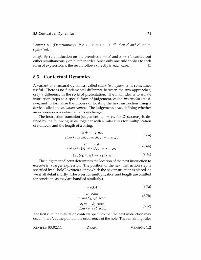
8.3 Contextual Dynamics 71
Lemma 8.2 (Determinacy). If e 53 e% and e 53 e%%, then e% and e%% are $-equivalent.
Proof. By rule induction on the premises e 53 e% and e 53 e%%, carried outeither simultaneously or in either order. Since only one rule applies to eachform of expression, e, the result follows directly in each case.
8.3 Contextual Dynamics
A variant of structural dynamics, called contextual dynamics, is sometimesuseful. There is no fundamental difference between the two approaches,only a difference in the style of presentation. The main idea is to isolateinstruction steps as a special form of judgement, called instruction transi-tion, and to formalize the process of locating the next instruction using adevice called an evaluation context. The judgement, e val, defining whetheran expression is a value, remains unchanged.
The instruction transition judgement, e1 ! e2, for L{num str} is de-fined by the following rules, together with similar rules for multiplicationof numbers and the length of a string.
m + n = p nat
plus(num[m]; num[n]) ! num[p] (8.6a)
s ˆ t = u strcat(str[s]; str[t]) ! str[u] (8.6b)
let(e1; x.e2) ! [e1/x]e2 (8.6c)
The judgement E ectxt determines the location of the next instruction toexecute in a larger expression. The position of the next instruction step isspecified by a “hole”, written 8, into which the next instruction is placed, aswe shall detail shortly. (The rules for multiplication and length are omittedfor concision, as they are handled similarly.)
8 ectxt (8.7a)
E1 ectxtplus(E1; e2) ectxt
(8.7b)
e1 val E2 ectxtplus(e1; E2) ectxt
(8.7c)
The first rule for evaluation contexts specifies that the next instruction mayoccur “here”, at the point of the occurrence of the hole. The remaining rules
REVISED 03.02.11 DRAFT VERSION 1.2
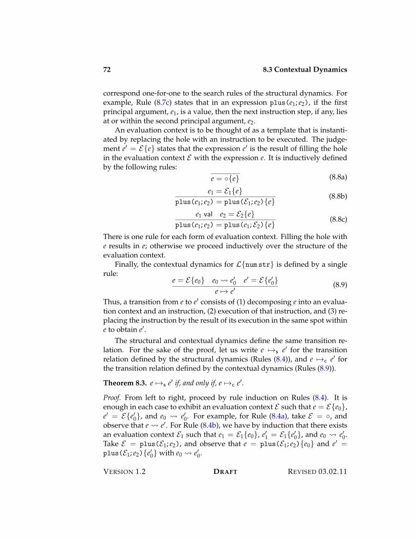
72 8.3 Contextual Dynamics
correspond one-for-one to the search rules of the structural dynamics. Forexample, Rule (8.7c) states that in an expression plus(e1; e2), if the firstprincipal argument, e1, is a value, then the next instruction step, if any, liesat or within the second principal argument, e2.
An evaluation context is to be thought of as a template that is instanti-ated by replacing the hole with an instruction to be executed. The judge-ment e% = E{e} states that the expression e% is the result of filling the holein the evaluation context E with the expression e. It is inductively definedby the following rules:
e = 8{e} (8.8a)
e1 = E1{e}plus(e1; e2) = plus(E1; e2){e}
(8.8b)
e1 val e2 = E2{e}plus(e1; e2) = plus(e1; E2){e}
(8.8c)
There is one rule for each form of evaluation context. Filling the hole withe results in e; otherwise we proceed inductively over the structure of theevaluation context.
Finally, the contextual dynamics for L{num str} is defined by a singlerule:
e = E{e0} e0 ! e%0 e% = E{e%0}e 53 e%
(8.9)
Thus, a transition from e to e% consists of (1) decomposing e into an evalua-tion context and an instruction, (2) execution of that instruction, and (3) re-placing the instruction by the result of its execution in the same spot withine to obtain e%.
The structural and contextual dynamics define the same transition re-lation. For the sake of the proof, let us write e 53s e% for the transitionrelation defined by the structural dynamics (Rules (8.4)), and e 53c e% forthe transition relation defined by the contextual dynamics (Rules (8.9)).
Theorem 8.3. e 53s e% if, and only if, e 53c e%.
Proof. From left to right, proceed by rule induction on Rules (8.4). It isenough in each case to exhibit an evaluation context E such that e = E{e0},e% = E{e%0}, and e0 ! e%0. For example, for Rule (8.4a), take E = 8, andobserve that e ! e%. For Rule (8.4b), we have by induction that there existsan evaluation context E1 such that e1 = E1{e0}, e%1 = E1{e%0}, and e0 ! e%0.Take E = plus(E1; e2), and observe that e = plus(E1; e2){e0} and e% =plus(E1; e2){e%0} with e0 ! e%0.
VERSION 1.2 DRAFT REVISED 03.02.11
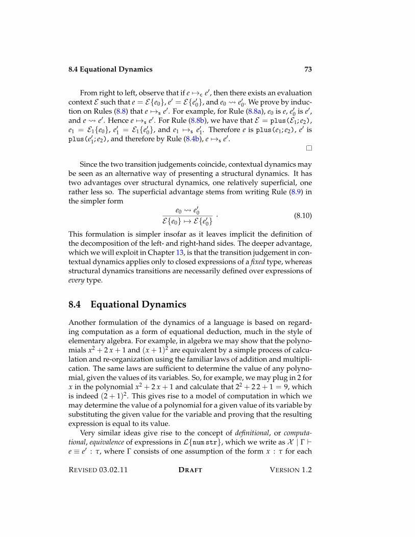
8.4 Equational Dynamics 73
From right to left, observe that if e 53c e%, then there exists an evaluationcontext E such that e = E{e0}, e% = E{e%0}, and e0 ! e%0. We prove by induc-tion on Rules (8.8) that e 53s e%. For example, for Rule (8.8a), e0 is e, e%0 is e%,and e ! e%. Hence e 53s e%. For Rule (8.8b), we have that E = plus(E1; e2),e1 = E1{e0}, e%1 = E1{e%0}, and e1 53s e%1. Therefore e is plus(e1; e2), e% isplus(e%1; e2), and therefore by Rule (8.4b), e 53s e%.
Since the two transition judgements coincide, contextual dynamics maybe seen as an alternative way of presenting a structural dynamics. It hastwo advantages over structural dynamics, one relatively superficial, onerather less so. The superficial advantage stems from writing Rule (8.9) inthe simpler form
e0 ! e%0E{e0} 53 E{e%0}
. (8.10)
This formulation is simpler insofar as it leaves implicit the definition ofthe decomposition of the left- and right-hand sides. The deeper advantage,which we will exploit in Chapter 13, is that the transition judgement in con-textual dynamics applies only to closed expressions of a fixed type, whereasstructural dynamics transitions are necessarily defined over expressions ofevery type.
8.4 Equational Dynamics
Another formulation of the dynamics of a language is based on regard-ing computation as a form of equational deduction, much in the style ofelementary algebra. For example, in algebra we may show that the polyno-mials x2 + 2 x + 1 and (x + 1)2 are equivalent by a simple process of calcu-lation and re-organization using the familiar laws of addition and multipli-cation. The same laws are sufficient to determine the value of any polyno-mial, given the values of its variables. So, for example, we may plug in 2 forx in the polynomial x2 + 2 x + 1 and calculate that 22 + 2 2 + 1 = 9, whichis indeed (2 + 1)2. This gives rise to a model of computation in which wemay determine the value of a polynomial for a given value of its variable bysubstituting the given value for the variable and proving that the resultingexpression is equal to its value.
Very similar ideas give rise to the concept of definitional, or computa-tional, equivalence of expressions in L{num str}, which we write as X | ! )e 9 e% : ", where ! consists of one assumption of the form x : " for each
REVISED 03.02.11 DRAFT VERSION 1.2
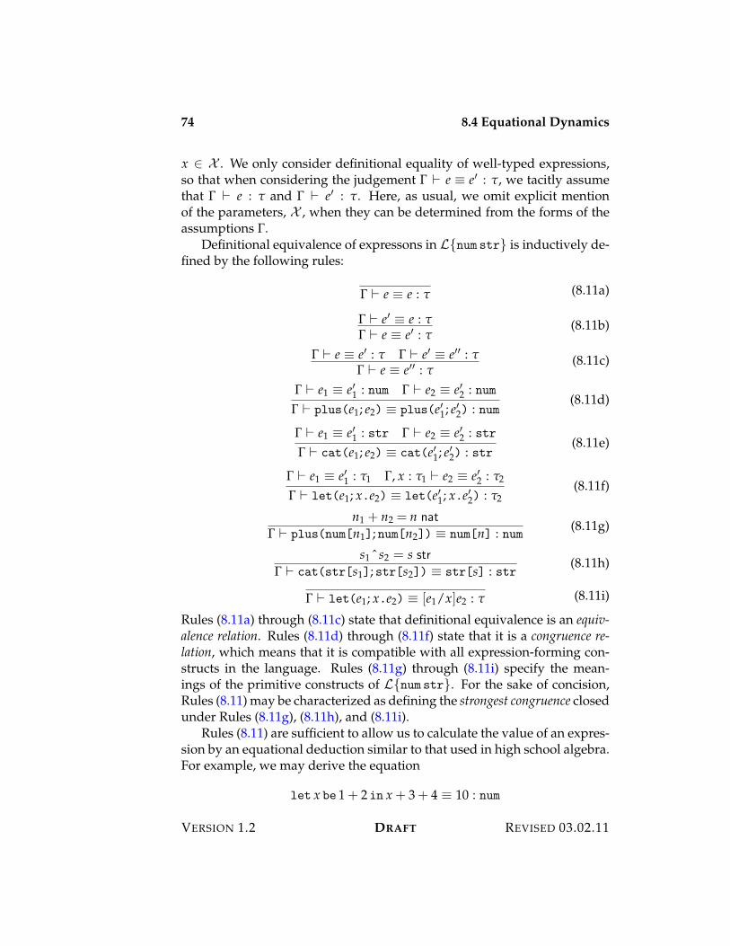
74 8.4 Equational Dynamics
x + X . We only consider definitional equality of well-typed expressions,so that when considering the judgement ! ) e 9 e% : ", we tacitly assumethat ! ) e : " and ! ) e% : ". Here, as usual, we omit explicit mentionof the parameters, X , when they can be determined from the forms of theassumptions !.
Definitional equivalence of expressons in L{num str} is inductively de-fined by the following rules:
! ) e 9 e : " (8.11a)
! ) e% 9 e : "! ) e 9 e% : "
(8.11b)
! ) e 9 e% : " ! ) e% 9 e%% : "! ) e 9 e%% : "
(8.11c)
! ) e1 9 e%1 : num ! ) e2 9 e%2 : num! ) plus(e1; e2) 9 plus(e%1; e%2) : num
(8.11d)
! ) e1 9 e%1 : str ! ) e2 9 e%2 : str! ) cat(e1; e2) 9 cat(e%1; e%2) : str
(8.11e)
! ) e1 9 e%1 : "1 !, x : "1 ) e2 9 e%2 : "2
! ) let(e1; x.e2) 9 let(e%1; x.e%2) : "2(8.11f)
n1 + n2 = n nat! ) plus(num[n1]; num[n2]) 9 num[n] : num (8.11g)
s1 ˆ s2 = s str! ) cat(str[s1]; str[s2]) 9 str[s] : str
(8.11h)
! ) let(e1; x.e2) 9 [e1/x]e2 : " (8.11i)
Rules (8.11a) through (8.11c) state that definitional equivalence is an equiv-alence relation. Rules (8.11d) through (8.11f) state that it is a congruence re-lation, which means that it is compatible with all expression-forming con-structs in the language. Rules (8.11g) through (8.11i) specify the mean-ings of the primitive constructs of L{num str}. For the sake of concision,Rules (8.11) may be characterized as defining the strongest congruence closedunder Rules (8.11g), (8.11h), and (8.11i).
Rules (8.11) are sufficient to allow us to calculate the value of an expres-sion by an equational deduction similar to that used in high school algebra.For example, we may derive the equation
let x be 1 + 2 in x + 3 + 4 9 10 : num
VERSION 1.2 DRAFT REVISED 03.02.11
8.4 Equational Dynamics 75
by applying Rules (8.11). Here, as in general, there may be many differentways to derive the same equation, but we need find only one derivation inorder to carry out an evaluation.
Definitional equivalence is rather weak in that many equivalences thatone might intuitively think are true are not derivable from Rules (8.11). Aprototypical example is the putative equivalence
x : num, y : num ) x1 + x2 9 x2 + x1 : num, (8.12)
which, intuitively, expresses the commutativity of addition. Although weshall not prove this here, this equivalence is not derivable from Rules (8.11).And yet we may derive all of its closed instances,
n1 + n2 9 n2 + n1 : num, (8.13)
where n1 nat and n2 nat are particular numbers.The “gap” between a general law, such as Equation (8.12), and all of its
instances, given by Equation (8.13), may be filled by enriching the notionof equivalence to include a principle of proof by mathematical induction.Such a notion of equivalence is sometimes called semantic, or observational,equivalence, since it expresses relationships that hold by virtue of the dy-namics of the expressions involved.2 Semantic equivalence is a syntheticjudgement, one that requires proof. It is to be distinguished from defini-tional equivalence, which expresses an analytic judgement, one that is self-evident based solely on the dynamics of the operations involved. As suchdefinitional equivalence may be thought of as symbolic evaluation, whichpermits simplification according to the evaluation rules of a language, butwhich does not permit reasoning by induction.
Definitional equivalence is adequate for evaluation in that it permits thecalculation of the value of any closed expression.
Theorem 8.4. e 9 e% : " iff there exists e0 val such that e 531 e0 and e% 531 e0.
Proof. The proof from right to left is direct, since every transition step isa valid equation. The converse follows from the following, more general,proposition. If x1 : "1, . . . , xn : "n ) e 9 e% : ", then whenever e1 : "1, . . . , en :"n, if
[e1, . . . , en/x1, . . . , xn]e 9 [e1, . . . , en/x1, . . . , xn]e% : ",
then there exists e0 val such that
[e1, . . . , en/x1, . . . , xn]e 531 e0
2This concept of equivalence is developed rigorously in Chapter 51.
REVISED 03.02.11 DRAFT VERSION 1.2
76 8.5 Exercises
and[e1, . . . , en/x1, . . . , xn]e% 531 e0.
This is proved by rule induction on Rules (8.11).
The formulation of definitional equivalence for the by-value dynamicsof binding requires a bit of additional machinery. The key idea is motivatedby the modifications required to Rule (8.11i) to express the requirement thate1 be a value. As a first cut one might consider simply adding an additionalpremise to the rule:
e1 val
! ) let(e1; x.e2) 9 [e1/x]e2 : "(8.14)
This is almost correct, except that the judgement e val is defined only forclosed expressions, whereas e1 might well involve free variables in !. Whatis required is to extend the judgement e val to the hypothetical judgement
x1 val, . . . , xn val ) e val
in which the hypotheses express the assumption that variables are onlyever bound to values, and hence can be regarded as values. To maintainthis invariant, we must maintain a set, %, of such hypotheses as part of def-initional equivalence, writing % ! ) e 9 e% : ", and modifying Rule (8.11f)as follows:
% ! ) e1 9 e%1 : "1 %, x val !, x : "1 ) e2 9 e%2 : "2
% ! ) let(e1; x.e2) 9 let(e%1; x.e%2) : "2(8.15)
The other rules are correspondingly modified to simply carry along % is anadditional set of hypotheses of the inference.
8.5 Exercises
1. For the structural dynamics of L{num str}, prove that if e 53 e1 ande 53 e2, then e1 =$ e2.
2. Formulate a variation of L{num str} with both a by-name and a by-value let construct.
VERSION 1.2 DRAFT REVISED 03.02.11
Chapter 9
Type Safety
Most contemporary programming languages are safe (or, type safe, or stronglytyped). Informally, this means that certain kinds of mismatches cannot ariseduring execution. For example, type safety for L{num str} states that it willnever arise that a number is to be added to a string, or that two numbersare to be concatenated, neither of which is meaningful.
In general type safety expresses the coherence between the statics andthe dynamics. The statics may be seen as predicting that the value of anexpression will have a certain form so that the dynamics of that expressionis well-defined. Consequently, evaluation cannot “get stuck” in a state forwhich no transition is possible, corresponding in implementation terms tothe absence of “illegal instruction” errors at execution time. This is provedby showing that each step of transition preserves typability and by showingthat typable states are well-defined. Consequently, evaluation can never“go off into the weeds,” and hence can never encounter an illegal instruc-tion.
More precisely, type safety for L{num str} may be stated as follows:
Theorem 9.1 (Type Safety). 1. If e : " and e 53 e%, then e% : ".
2. If e : ", then either e val, or there exists e% such that e 53 e%.
The first part, called preservation, says that the steps of evaluation pre-serve typing; the second, called progress, ensures that well-typed expres-sions are either values or can be further evaluated. Safety is the conjunctionof preservation and progress.
We say that an expression, e, is stuck iff it is not a value, yet there is noe% such that e 53 e%. It follows from the safety theorem that a stuck state is
78 9.1 Preservation
necessarily ill-typed. Or, putting it the other way around, that well-typedstates do not get stuck.
9.1 Preservation
The preservation theorem for L{num str} defined in Chapters 7 and 8 isproved by rule induction on the transition system (rules (8.4)).
Theorem 9.2 (Preservation). If e : " and e 53 e%, then e% : ".
Proof. We will consider two cases, leaving the rest to the reader. Considerrule (8.4b),
e1 53 e%1plus(e1; e2) 53 plus(e%1; e2)
.
Assume that plus(e1; e2) : ". By inversion for typing, we have that " =num, e1 : num, and e2 : num. By induction we have that e%1 : num, and henceplus(e%1; e2) : num. The case for concatenation is handled similarly.
Now consider rule (8.4g),
e1 val
let(e1; x.e2) 53 [e1/x]e2.
Assume that let(e1; x.e2) : "2. By the inversion lemma 7.2 on page 64,e1 : "1 for some "1 such that x : "1 ) e2 : "2. By the substitution lemma 7.4on page 64 [e1/x]e2 : "2, as desired.
The proof of preservation is naturally structured as an induction on thetransition judgement, since the argument hinges on examining all possibletransitions from a given expression. In some cases one may manage tocarry out a proof by structural induction on e, or by an induction on typing,but experience shows that this often leads to awkward arguments, or, insome cases, cannot be made to work at all.
9.2 Progress
The progress theorem captures the idea that well-typed programs cannot“get stuck”. The proof depends crucially on the following lemma, whichcharacterizes the values of each type.
Lemma 9.3 (Canonical Forms). If e val and e : ", then
VERSION 1.2 DRAFT REVISED 03.02.11
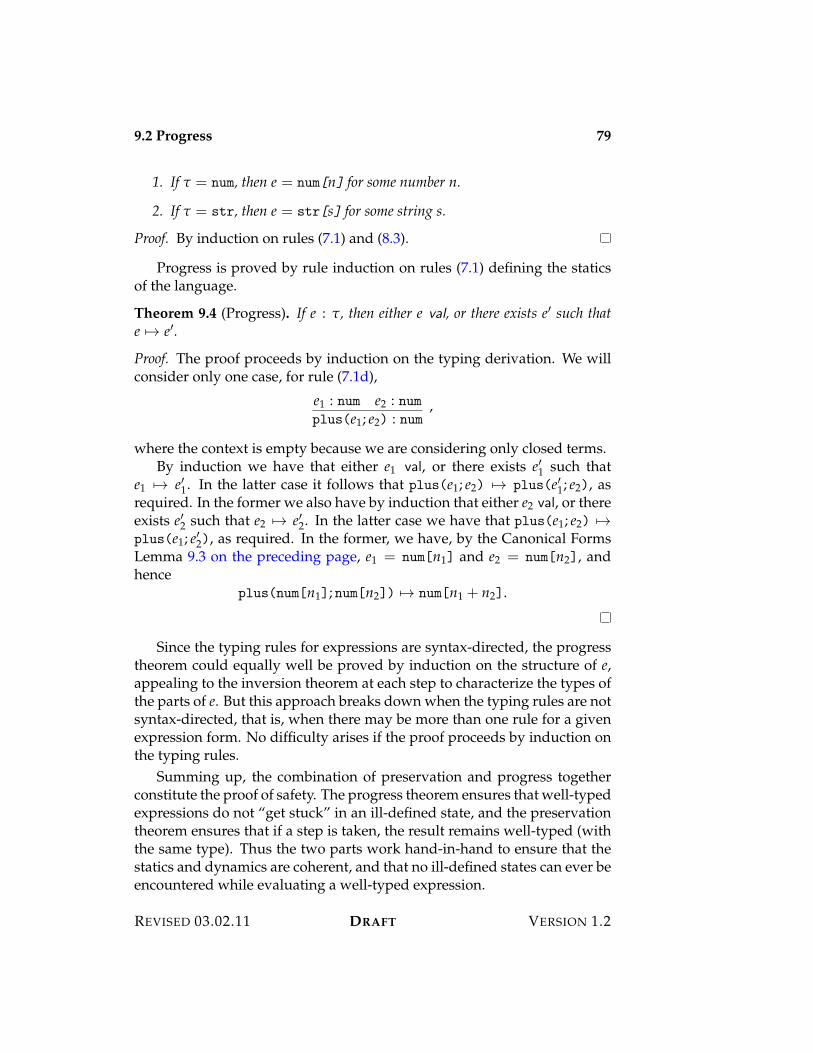
9.2 Progress 79
1. If " = num, then e = num[n] for some number n.
2. If " = str, then e = str[s] for some string s.
Proof. By induction on rules (7.1) and (8.3).
Progress is proved by rule induction on rules (7.1) defining the staticsof the language.
Theorem 9.4 (Progress). If e : ", then either e val, or there exists e% such thate 53 e%.
Proof. The proof proceeds by induction on the typing derivation. We willconsider only one case, for rule (7.1d),
e1 : num e2 : numplus(e1; e2) : num
,
where the context is empty because we are considering only closed terms.By induction we have that either e1 val, or there exists e%1 such that
e1 53 e%1. In the latter case it follows that plus(e1; e2) 53 plus(e%1; e2), asrequired. In the former we also have by induction that either e2 val, or thereexists e%2 such that e2 53 e%2. In the latter case we have that plus(e1; e2) 53plus(e1; e%2), as required. In the former, we have, by the Canonical FormsLemma 9.3 on the preceding page, e1 = num[n1] and e2 = num[n2], andhence
plus(num[n1]; num[n2]) 53 num[n1 + n2].
Since the typing rules for expressions are syntax-directed, the progresstheorem could equally well be proved by induction on the structure of e,appealing to the inversion theorem at each step to characterize the types ofthe parts of e. But this approach breaks down when the typing rules are notsyntax-directed, that is, when there may be more than one rule for a givenexpression form. No difficulty arises if the proof proceeds by induction onthe typing rules.
Summing up, the combination of preservation and progress togetherconstitute the proof of safety. The progress theorem ensures that well-typedexpressions do not “get stuck” in an ill-defined state, and the preservationtheorem ensures that if a step is taken, the result remains well-typed (withthe same type). Thus the two parts work hand-in-hand to ensure that thestatics and dynamics are coherent, and that no ill-defined states can ever beencountered while evaluating a well-typed expression.
REVISED 03.02.11 DRAFT VERSION 1.2
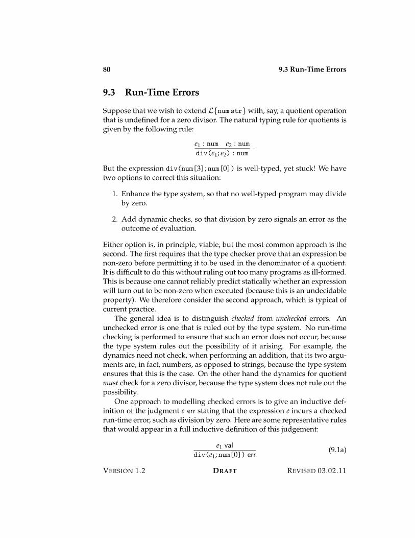
80 9.3 Run-Time Errors
9.3 Run-Time Errors
Suppose that we wish to extend L{num str} with, say, a quotient operationthat is undefined for a zero divisor. The natural typing rule for quotients isgiven by the following rule:
e1 : num e2 : numdiv(e1; e2) : num
.
But the expression div(num[3]; num[0]) is well-typed, yet stuck! We havetwo options to correct this situation:
1. Enhance the type system, so that no well-typed program may divideby zero.
2. Add dynamic checks, so that division by zero signals an error as theoutcome of evaluation.
Either option is, in principle, viable, but the most common approach is thesecond. The first requires that the type checker prove that an expression benon-zero before permitting it to be used in the denominator of a quotient.It is difficult to do this without ruling out too many programs as ill-formed.This is because one cannot reliably predict statically whether an expressionwill turn out to be non-zero when executed (because this is an undecidableproperty). We therefore consider the second approach, which is typical ofcurrent practice.
The general idea is to distinguish checked from unchecked errors. Anunchecked error is one that is ruled out by the type system. No run-timechecking is performed to ensure that such an error does not occur, becausethe type system rules out the possibility of it arising. For example, thedynamics need not check, when performing an addition, that its two argu-ments are, in fact, numbers, as opposed to strings, because the type systemensures that this is the case. On the other hand the dynamics for quotientmust check for a zero divisor, because the type system does not rule out thepossibility.
One approach to modelling checked errors is to give an inductive def-inition of the judgment e err stating that the expression e incurs a checkedrun-time error, such as division by zero. Here are some representative rulesthat would appear in a full inductive definition of this judgement:
e1 valdiv(e1; num[0]) err
(9.1a)
VERSION 1.2 DRAFT REVISED 03.02.11
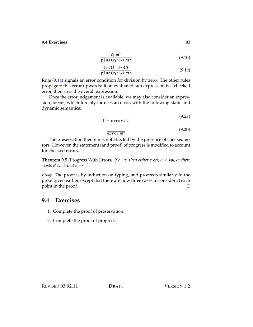
9.4 Exercises 81
e1 errplus(e1; e2) err (9.1b)
e1 val e2 errplus(e1; e2) err
(9.1c)
Rule (9.1a) signals an error condition for division by zero. The other rulespropagate this error upwards: if an evaluated sub-expression is a checkederror, then so is the overall expression.
Once the error judgement is available, we may also consider an expres-sion, error, which forcibly induces an error, with the following static anddynamic semantics:
! ) error : "(9.2a)
error err(9.2b)
The preservation theorem is not affected by the presence of checked er-rors. However, the statement (and proof) of progress is modified to accountfor checked errors.
Theorem 9.5 (Progress With Error). If e : ", then either e err, or e val, or thereexists e% such that e 53 e%.
Proof. The proof is by induction on typing, and proceeds similarly to theproof given earlier, except that there are now three cases to consider at eachpoint in the proof.
9.4 Exercises
1. Complete the proof of preservation.
2. Complete the proof of progress.
REVISED 03.02.11 DRAFT VERSION 1.2

82 9.4 Exercises
VERSION 1.2 DRAFT REVISED 03.02.11
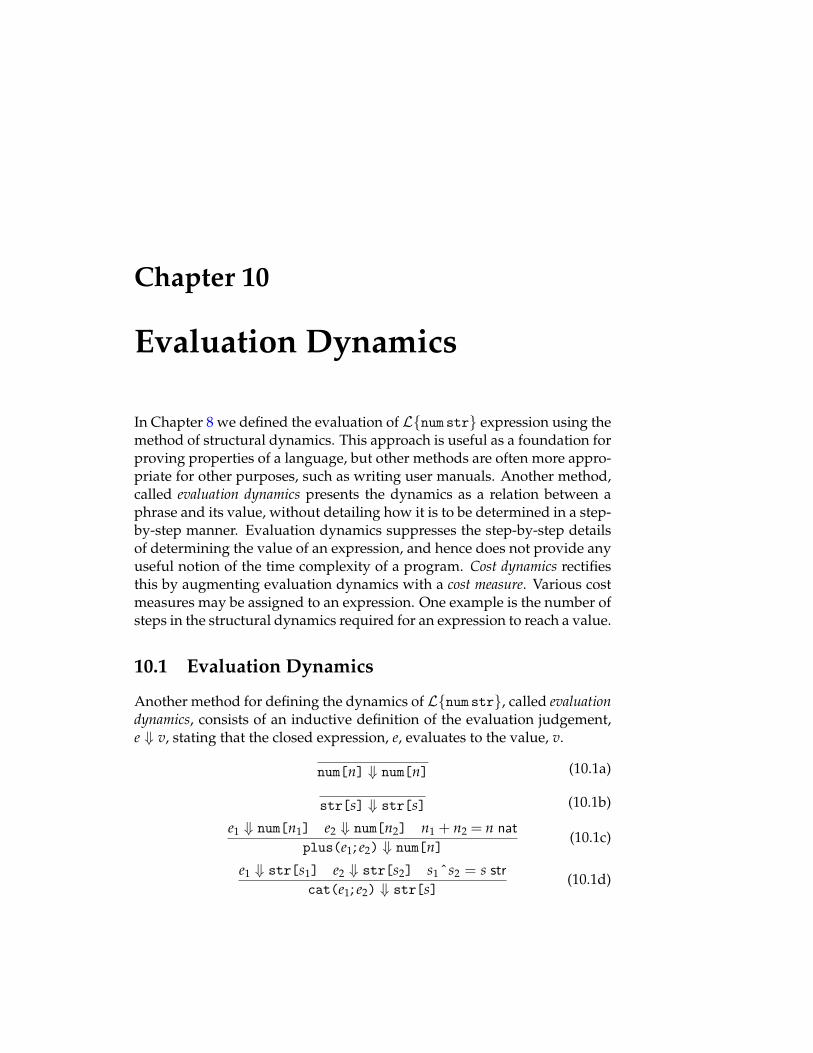
Chapter 10
Evaluation Dynamics
In Chapter 8 we defined the evaluation of L{num str} expression using themethod of structural dynamics. This approach is useful as a foundation forproving properties of a language, but other methods are often more appro-priate for other purposes, such as writing user manuals. Another method,called evaluation dynamics presents the dynamics as a relation between aphrase and its value, without detailing how it is to be determined in a step-by-step manner. Evaluation dynamics suppresses the step-by-step detailsof determining the value of an expression, and hence does not provide anyuseful notion of the time complexity of a program. Cost dynamics rectifiesthis by augmenting evaluation dynamics with a cost measure. Various costmeasures may be assigned to an expression. One example is the number ofsteps in the structural dynamics required for an expression to reach a value.
10.1 Evaluation Dynamics
Another method for defining the dynamics of L{num str}, called evaluationdynamics, consists of an inductive definition of the evaluation judgement,e " v, stating that the closed expression, e, evaluates to the value, v.
num[n] " num[n] (10.1a)
str[s] " str[s] (10.1b)
e1 " num[n1] e2 " num[n2] n1 + n2 = n natplus(e1; e2) " num[n]
(10.1c)
e1 " str[s1] e2 " str[s2] s1 ˆ s2 = s strcat(e1; e2) " str[s]
(10.1d)

84 10.2 Relating Structural and Evaluation Dynamics
e " str[s] |s| = n str
len(e) " num[n](10.1e)
[e1/x]e2 " v2
let(e1; x.e2) " v2(10.1f)
The value of a let expression is determined by substitution of the bindinginto the body. The rules are therefore not syntax-directed, since the premiseof Rule (10.1f) is not a sub-expression of the expression in the conclusion ofthat rule.
The evaluation judgement is inductively defined, we prove propertiesof it by rule induction. Specifically, to show that the property P(e " v)holds, it is enough to show that P is closed under Rules (10.1):
1. Show that P(num[n] " num[n]).
2. Show that P(str[s] " str[s]).
3. Show that P(plus(e1; e2) " num[n]), if P(e1 " num[n1]), P(e2 " num[n2]),and n1 + n2 = n nat.
4. Show that P(cat(e1; e2) " str[s]), if P(e1 " str[s1]), P(e2 " str[s2]),and s1 ˆ s2 = s str.
5. Show that P(let(e1; x.e2) " v2), if P([e1/x]e2 " v2).
This induction principle is not the same as structural induction on e exp,because the evaluation rules are not syntax-directed!
Lemma 10.1. If e " v, then v val.
Proof. By induction on Rules (10.1). All cases except Rule (10.1f) are im-mediate. For the latter case, the result follows directly by an appeal to theinductive hypothesis for the second premise of the evaluation rule.
10.2 Relating Structural and Evaluation Dynamics
We have given two different forms of dynamics for L{num str}. It is nat-ural to ask whether they are equivalent, but to do so first requires that weconsider carefully what we mean by equivalence. The structural dynamicsdescribes a step-by-step process of execution, whereas the evaluation dy-namics suppresses the intermediate states, focussing attention on the initialand final states alone. This suggests that the appropriate correspondence
VERSION 1.2 DRAFT REVISED 03.02.11
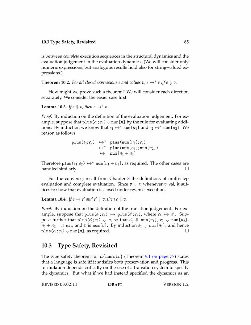
10.3 Type Safety, Revisited 85
is between complete execution sequences in the structural dynamics and theevaluation judgement in the evaluation dynamics. (We will consider onlynumeric expressions, but analogous results hold also for string-valued ex-pressions.)
Theorem 10.2. For all closed expressions e and values v, e 531 v iff e " v.
How might we prove such a theorem? We will consider each directionseparately. We consider the easier case first.
Lemma 10.3. If e " v, then e 531 v.
Proof. By induction on the definition of the evaluation judgement. For ex-ample, suppose that plus(e1; e2) " num[n] by the rule for evaluating addi-tions. By induction we know that e1 531 num[n1] and e2 531 num[n2]. Wereason as follows:
plus(e1; e2) 531 plus(num[n1]; e2)
531 plus(num[n1]; num[n2])
53 num[n1 + n2]
Therefore plus(e1; e2) 531 num[n1 + n2], as required. The other cases arehandled similarly.
For the converse, recall from Chapter 8 the definitions of multi-stepevaluation and complete evaluation. Since v " v whenever v val, it suf-fices to show that evaluation is closed under reverse execution.
Lemma 10.4. If e 53 e% and e% " v, then e " v.
Proof. By induction on the definition of the transition judgement. For ex-ample, suppose that plus(e1; e2) 53 plus(e%1; e2), where e1 53 e%1. Sup-pose further that plus(e%1; e2) " v, so that e%1 " num[n1], e2 " num[n2],n1 + n2 = n nat, and v is num[n]. By induction e1 " num[n1], and henceplus(e1; e2) " num[n], as required.
10.3 Type Safety, Revisited
The type safety theorem for L{num str} (Theorem 9.1 on page 77) statesthat a language is safe iff it satisfies both preservation and progress. Thisformulation depends critically on the use of a transition system to specifythe dynamics. But what if we had instead specified the dynamics as an
REVISED 03.02.11 DRAFT VERSION 1.2
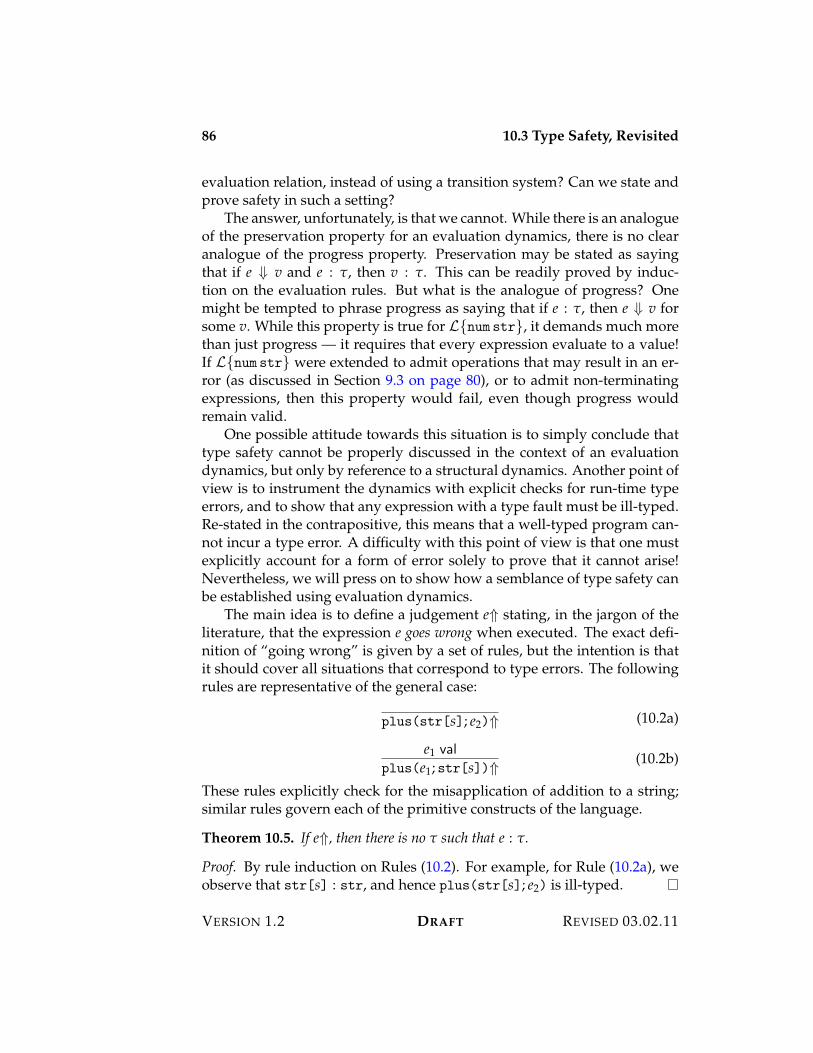
86 10.3 Type Safety, Revisited
evaluation relation, instead of using a transition system? Can we state andprove safety in such a setting?
The answer, unfortunately, is that we cannot. While there is an analogueof the preservation property for an evaluation dynamics, there is no clearanalogue of the progress property. Preservation may be stated as sayingthat if e " v and e : ", then v : ". This can be readily proved by induc-tion on the evaluation rules. But what is the analogue of progress? Onemight be tempted to phrase progress as saying that if e : ", then e " v forsome v. While this property is true for L{num str}, it demands much morethan just progress — it requires that every expression evaluate to a value!If L{num str} were extended to admit operations that may result in an er-ror (as discussed in Section 9.3 on page 80), or to admit non-terminatingexpressions, then this property would fail, even though progress wouldremain valid.
One possible attitude towards this situation is to simply conclude thattype safety cannot be properly discussed in the context of an evaluationdynamics, but only by reference to a structural dynamics. Another point ofview is to instrument the dynamics with explicit checks for run-time typeerrors, and to show that any expression with a type fault must be ill-typed.Re-stated in the contrapositive, this means that a well-typed program can-not incur a type error. A difficulty with this point of view is that one mustexplicitly account for a form of error solely to prove that it cannot arise!Nevertheless, we will press on to show how a semblance of type safety canbe established using evaluation dynamics.
The main idea is to define a judgement e: stating, in the jargon of theliterature, that the expression e goes wrong when executed. The exact defi-nition of “going wrong” is given by a set of rules, but the intention is thatit should cover all situations that correspond to type errors. The followingrules are representative of the general case:
plus(str[s]; e2): (10.2a)
e1 valplus(e1; str[s]): (10.2b)
These rules explicitly check for the misapplication of addition to a string;similar rules govern each of the primitive constructs of the language.
Theorem 10.5. If e:, then there is no " such that e : ".
Proof. By rule induction on Rules (10.2). For example, for Rule (10.2a), weobserve that str[s] : str, and hence plus(str[s]; e2) is ill-typed.
VERSION 1.2 DRAFT REVISED 03.02.11
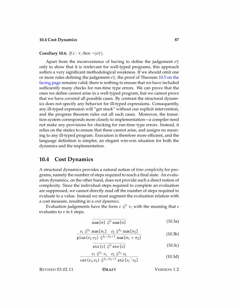
10.4 Cost Dynamics 87
Corollary 10.6. If e : ", then ¬(e:).
Apart from the inconvenience of having to define the judgement e:only to show that it is irrelevant for well-typed programs, this approachsuffers a very significant methodological weakness. If we should omit oneor more rules defining the judgement e:, the proof of Theorem 10.5 on thefacing page remains valid; there is nothing to ensure that we have includedsufficiently many checks for run-time type errors. We can prove that theones we define cannot arise in a well-typed program, but we cannot provethat we have covered all possible cases. By contrast the structural dynam-ics does not specify any behavior for ill-typed expressions. Consequently,any ill-typed expression will “get stuck” without our explicit intervention,and the progress theorem rules out all such cases. Moreover, the transi-tion system corresponds more closely to implementation—a compiler neednot make any provisions for checking for run-time type errors. Instead, itrelies on the statics to ensure that these cannot arise, and assigns no mean-ing to any ill-typed program. Execution is therefore more efficient, and thelanguage definition is simpler, an elegant win-win situation for both thedynamics and the implementation.
10.4 Cost Dynamics
A structural dynamics provides a natural notion of time complexity for pro-grams, namely the number of steps required to reach a final state. An evalu-ation dynamics, on the other hand, does not provide such a direct notion ofcomplexity. Since the individual steps required to complete an evaluationare suppressed, we cannot directly read off the number of steps required toevaluate to a value. Instead we must augment the evaluation relation witha cost measure, resulting in a cost dynamics.
Evaluation judgements have the form e "k v, with the meaning that eevaluates to v in k steps.
num[n] "0 num[n] (10.3a)
e1 "k1 num[n1] e2 "k2 num[n2]
plus(e1; e2) "k1+k2+1 num[n1 + n2](10.3b)
str[s] "0 str[s] (10.3c)
e1 "k1 s1 e2 "k2 s2
cat(e1; e2) "k1+k2+1 str[s1 ˆ s2](10.3d)
REVISED 03.02.11 DRAFT VERSION 1.2
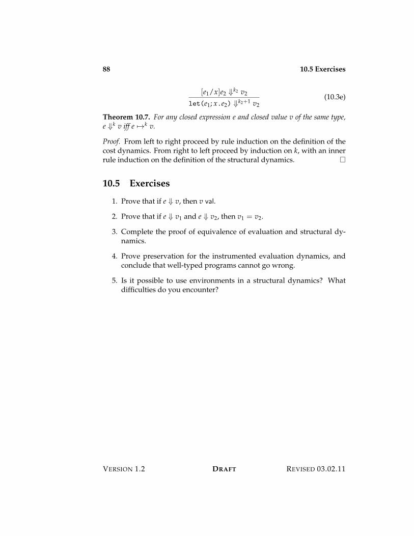
88 10.5 Exercises
[e1/x]e2 "k2 v2
let(e1; x.e2) "k2+1 v2(10.3e)
Theorem 10.7. For any closed expression e and closed value v of the same type,e "k v iff e 53k v.
Proof. From left to right proceed by rule induction on the definition of thecost dynamics. From right to left proceed by induction on k, with an innerrule induction on the definition of the structural dynamics.
10.5 Exercises
1. Prove that if e " v, then v val.
2. Prove that if e " v1 and e " v2, then v1 = v2.
3. Complete the proof of equivalence of evaluation and structural dy-namics.
4. Prove preservation for the instrumented evaluation dynamics, andconclude that well-typed programs cannot go wrong.
5. Is it possible to use environments in a structural dynamics? Whatdifficulties do you encounter?
VERSION 1.2 DRAFT REVISED 03.02.11
Part IV
Function Types

Chapter 11
Function Definitions andValues
In the language L{num str} we may perform calculations such as the dou-bling of a given expression, but we cannot express doubling as a conceptin itself. To capture the general pattern of doubling, we abstract away fromthe particular number being doubled using a variable to stand for a fixed,but unspecified, number, to express the doubling of an arbitrary number.Any particular instance of doubling may then be obtained by substituting anumeric expression for that variable. In general an expression may involvemany distinct variables, necessitating that we specify which of several pos-sible variables is varying in a particular context, giving rise to a function ofthat variable.
In this chapter we will consider two extensions of L{num str} withfunctions. The first, and perhaps most obvious, extension is by adding func-tion definitions to the language. A function is defined by binding a name toan abt with a bound variable that serves as the argument of that function. Afunction is applied by substituting a particular expression (of suitable type)for the bound variable, obtaining an expression.
The domain and range of defined functions are limited to the types natand str, since these are the only types of expression. Such functions arecalled first-order functions, in contrast to higher-order functions, which permitfunctions as arguments and results of other functions. Since the domainand range of a function are types, this requires that we introduce functiontypes whose elements are functions. Consequently, we may form functionsof higher type, those whose domain and range may themselves be functiontypes.
92 11.1 First-Order Functions
Historically the introduction of higher-order functions was responsiblefor a mistake in language design that subsequently was re-characterized asa feature, called dynamic binding. Dynamic binding arises from getting thedefinition of substitution wrong by failing to avoid capture. This makes thenames of bound variables important, in violation of the fundamental prin-ciple of binding stating that the names of bound variables are unimportant.
11.1 First-Order Functions
The language L{num str fun} is the extension of L{num str} with functiondefinitions and function applications as described by the following gram-mar:
Expr e ::= call[ f](e) f(e) callfun["1; "2](x1.e2; f.e) fun f(x1:"1):"2 = e2 in e definition
The expression fun["1; "2](x1.e2; f.e) binds the function name f withine to the pattern x1.e2, which has parameter x1 and definition e2. The do-main and range of the function are, respectively, the types "1 and "2. Theexpression call[ f](e) instantiates the binding of f with the argument e.
The statics of L{num str fun} defines two forms of judgement:
1. Expression typing, e : ", stating that e has type ";
2. Function typing, f("1) : "2, stating that f is a function with argumenttype "1 and result type "2.
The judgment f("1) : "2 is called the function header of f ; it specifies thedomain type and the range type of a function.
The statics of L{num str fun} is defined by the following rules:
!, x1 : "1 ) e2 : "2 !, f("1) : "2 ) e : "
! ) fun["1; "2](x1.e2; f.e) : "(11.1a)
! ) f("1) : "2 ! ) e : "1
! ) call[ f](e) : "2(11.1b)
Function substitution, written [[x.e/ f ]]e%, is defined by induction on thestructure of e% much like the definition of ordinary substitution. However,a function name, f , is not a form of expression, but rather can only occur in
VERSION 1.2 DRAFT REVISED 03.02.11
11.2 Higher-Order Functions 93
a call of the form call[ f](e). Function substitution for such expressions isdefined by the following rule:
[[x.e/ f ]]call[ f](e%) = let(e%; x.e)(11.2)
At call sites to f with argument e%, function substitution yields a let ex-pression that binds x to e% within e.
Lemma 11.1. If !, f("1) : "2 ) e : " and !, x1 : "2 ) e2 : "2, then ! )[[x1.e2/ f ]]e : ".
Proof. By induction on the structure of e%.
The dynamics of L{num str fun} is defined using function substitution:
fun["1; "2](x1.e2; f.e) 53 [[x1.e2/ f ]]e(11.3)
Since function substitution replaces all calls to f by appropriate let expres-sions, there is no need to give a rule for function calls.
The safety of L{num str fun} may be obtained as an immediate corol-lary of the safety theorem for higher-order functions, which we discussnext.
11.2 Higher-Order Functions
The syntactic and semantic similarity between variable definitions and func-tion definitions in L{num str fun} is striking. This suggests that it may bepossible to consolidate the two concepts into a single definition mechanism.The gap that must be bridged is the segregation of functions from expres-sions. A function name f is bound to an abstractor x.e specifying a patternthat is instantiated when f is applied. To consolidate function definitionswith expression definitions it is sufficient to reify the abstractor into a formof expression, called a !-abstraction, written lam["1](x.e). Correspond-ingly, we must generalize application to have the form ap(e1; e2), where e1is any expression, and not just a function name. These are, respectively, theintroduction and elimination forms for the function type, arr("1; "2), whoseelements are functions with domain "1 and range "2.
REVISED 03.02.11 DRAFT VERSION 1.2
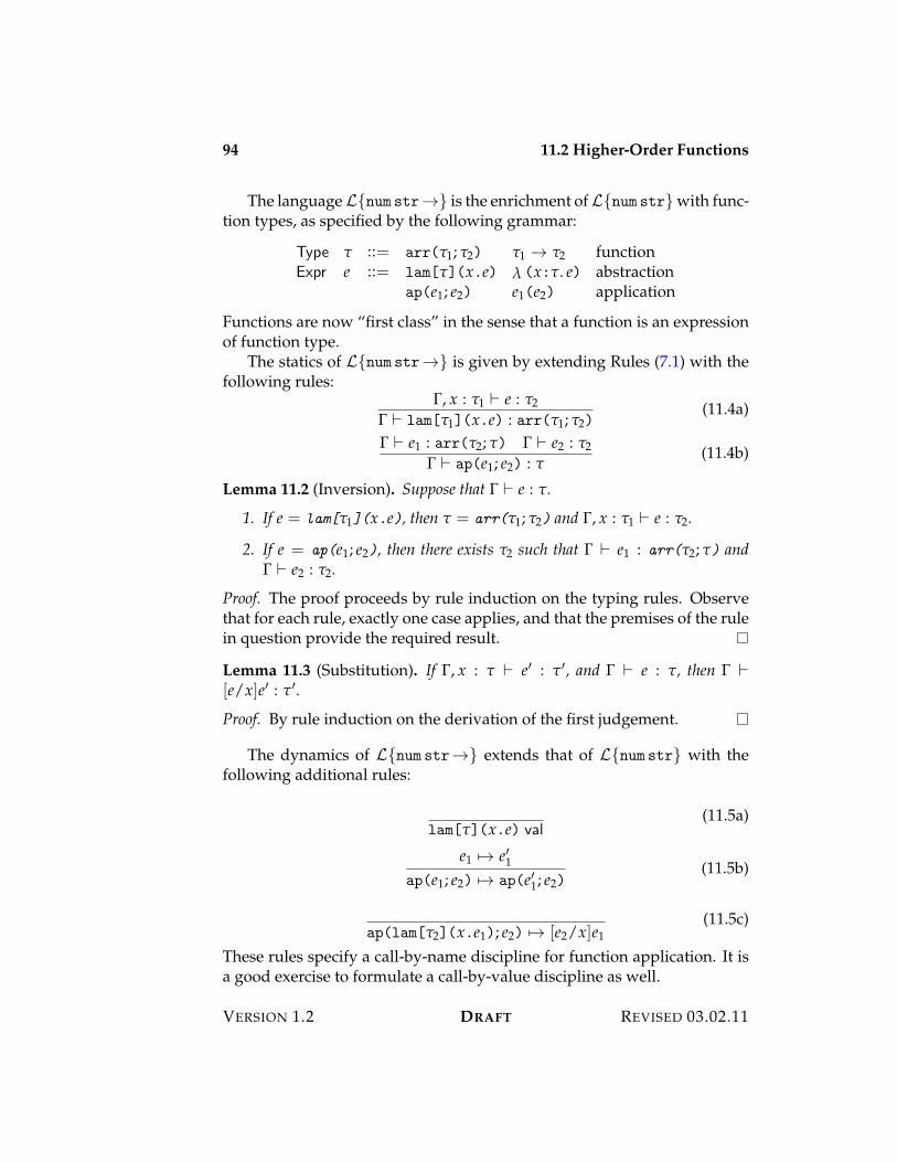
94 11.2 Higher-Order Functions
The language L{num str3} is the enrichment of L{num str} with func-tion types, as specified by the following grammar:
Type " ::= arr("1; "2) "1 3 "2 functionExpr e ::= lam["](x.e) ! (x:". e) abstraction
ap(e1; e2) e1(e2) application
Functions are now “first class” in the sense that a function is an expressionof function type.
The statics of L{num str3} is given by extending Rules (7.1) with thefollowing rules:
!, x : "1 ) e : "2! ) lam["1](x.e) : arr("1; "2)
(11.4a)
! ) e1 : arr("2; ") ! ) e2 : "2! ) ap(e1; e2) : "
(11.4b)
Lemma 11.2 (Inversion). Suppose that ! ) e : ".
1. If e = lam["1](x.e), then " = arr("1; "2) and !, x : "1 ) e : "2.
2. If e = ap(e1; e2), then there exists "2 such that ! ) e1 : arr("2; ") and! ) e2 : "2.
Proof. The proof proceeds by rule induction on the typing rules. Observethat for each rule, exactly one case applies, and that the premises of the rulein question provide the required result.
Lemma 11.3 (Substitution). If !, x : " ) e% : "%, and ! ) e : ", then ! )[e/x]e% : "%.
Proof. By rule induction on the derivation of the first judgement.
The dynamics of L{num str3} extends that of L{num str} with thefollowing additional rules:
lam["](x.e) val(11.5a)
e1 53 e%1ap(e1; e2) 53 ap(e%1; e2)
(11.5b)
ap(lam["2](x.e1); e2) 53 [e2/x]e1(11.5c)
These rules specify a call-by-name discipline for function application. It isa good exercise to formulate a call-by-value discipline as well.
VERSION 1.2 DRAFT REVISED 03.02.11
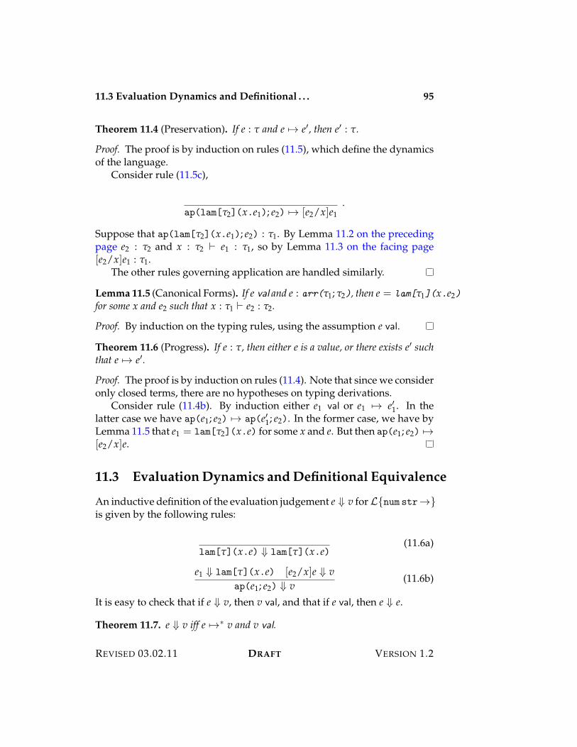
11.3 Evaluation Dynamics and Definitional . . . 95
Theorem 11.4 (Preservation). If e : " and e 53 e%, then e% : ".
Proof. The proof is by induction on rules (11.5), which define the dynamicsof the language.
Consider rule (11.5c),
ap(lam["2](x.e1); e2) 53 [e2/x]e1.
Suppose that ap(lam["2](x.e1); e2) : "1. By Lemma 11.2 on the precedingpage e2 : "2 and x : "2 ) e1 : "1, so by Lemma 11.3 on the facing page[e2/x]e1 : "1.
The other rules governing application are handled similarly.
Lemma 11.5 (Canonical Forms). If e val and e : arr("1; "2), then e = lam["1](x.e2)
for some x and e2 such that x : "1 ) e2 : "2.
Proof. By induction on the typing rules, using the assumption e val.
Theorem 11.6 (Progress). If e : ", then either e is a value, or there exists e% suchthat e 53 e%.
Proof. The proof is by induction on rules (11.4). Note that since we consideronly closed terms, there are no hypotheses on typing derivations.
Consider rule (11.4b). By induction either e1 val or e1 53 e%1. In thelatter case we have ap(e1; e2) 53 ap(e%1; e2). In the former case, we have byLemma 11.5 that e1 = lam["2](x.e) for some x and e. But then ap(e1; e2) 53[e2/x]e.
11.3 Evaluation Dynamics and Definitional Equivalence
An inductive definition of the evaluation judgement e " v for L{num str3}is given by the following rules:
lam["](x.e) " lam["](x.e)(11.6a)
e1 " lam["](x.e) [e2/x]e " vap(e1; e2) " v
(11.6b)
It is easy to check that if e " v, then v val, and that if e val, then e " e.
Theorem 11.7. e " v iff e 531 v and v val.
REVISED 03.02.11 DRAFT VERSION 1.2
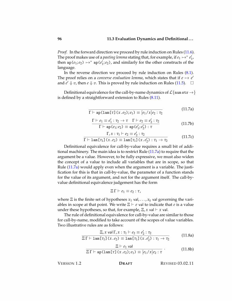
96 11.3 Evaluation Dynamics and Definitional . . .
Proof. In the forward direction we proceed by rule induction on Rules (11.6).The proof makes use of a pasting lemma stating that, for example, if e1 531 e%1,then ap(e1; e2) 531 ap(e%1; e2), and similarly for the other constructs of thelanguage.
In the reverse direction we proceed by rule induction on Rules (8.1).The proof relies on a converse evaluation lemma, which states that if e 53 e%and e% " v, then e " v. This is proved by rule induction on Rules (11.5).
Definitional equivalence for the call-by-name dynamics of L{num str3}is defined by a straightforward extension to Rules (8.11).
! ) ap(lam["](x.e2); e1) 9 [e1/x]e2 : "2(11.7a)
! ) e1 9 e%1 : "2 3 " ! ) e2 9 e%2 : "2
! ) ap(e1; e2) 9 ap(e%1; e%2) : "(11.7b)
!, x : "1 ) e2 9 e%2 : "2
! ) lam["1](x.e2) 9 lam["1](x.e%2) : "1 3 "2(11.7c)
Definitional equivalence for call-by-value requires a small bit of addi-tional machinery. The main idea is to restrict Rule (11.7a) to require that theargument be a value. However, to be fully expressive, we must also widenthe concept of a value to include all variables that are in scope, so thatRule (11.7a) would apply even when the argument is a variable. The justi-fication for this is that in call-by-value, the parameter of a function standsfor the value of its argument, and not for the argument itself. The call-by-value definitional equivalence judgement has the form
% ! ) e1 9 e2 : ",
where % is the finite set of hypotheses x1 val, . . . , xk val governing the vari-ables in scope at that point. We write % ) e val to indicate that e is a valueunder these hypotheses, so that, for example, %, x val ) x val.
The rule of definitional equivalence for call-by-value are similar to thosefor call-by-name, modified to take account of the scopes of value variables.Two illustrative rules are as follows:
%, x val !, x : "1 ) e2 9 e%2 : "2
% ! ) lam["1](x.e2) 9 lam["1](x.e%2) : "1 3 "2(11.8a)
% ) e1 val
% ! ) ap(lam["](x.e2); e1) 9 [e1/x]e2 : ". (11.8b)
VERSION 1.2 DRAFT REVISED 03.02.11
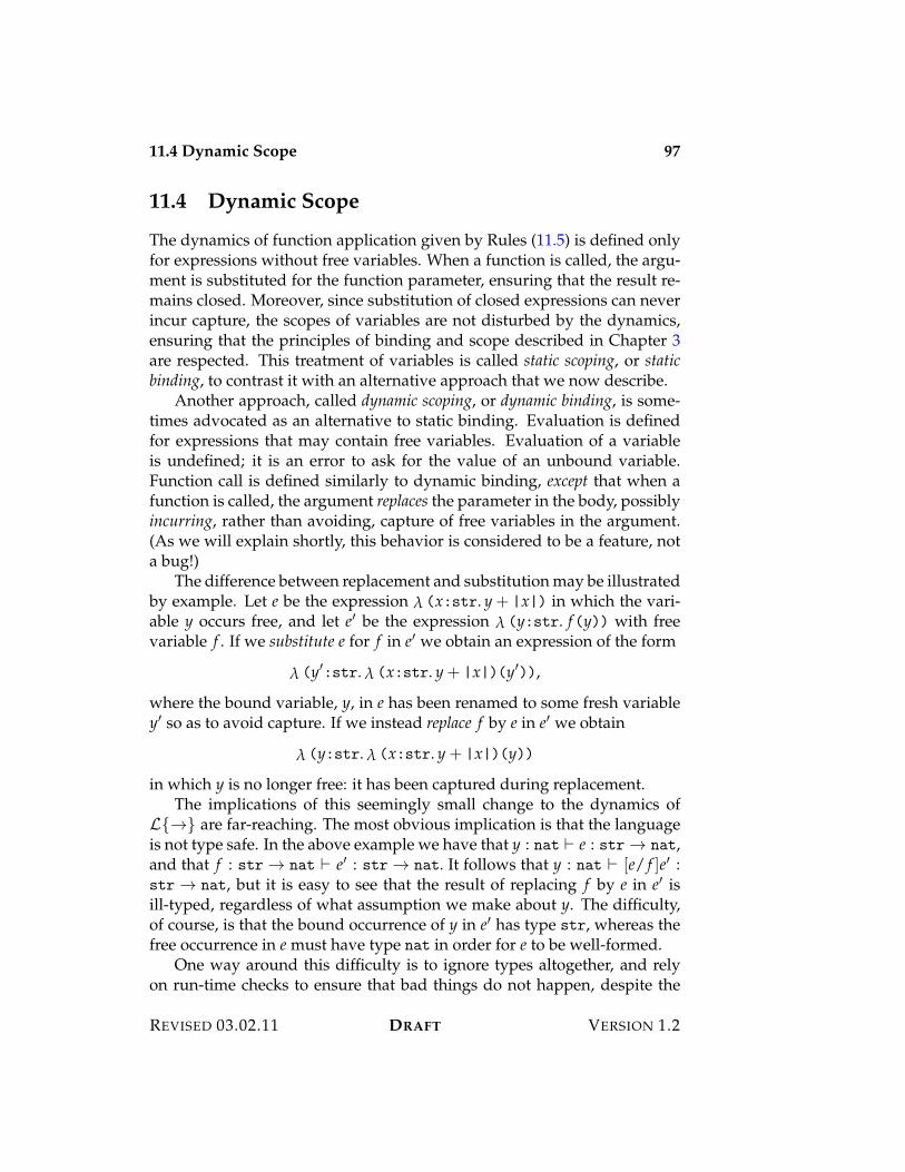
11.4 Dynamic Scope 97
11.4 Dynamic Scope
The dynamics of function application given by Rules (11.5) is defined onlyfor expressions without free variables. When a function is called, the argu-ment is substituted for the function parameter, ensuring that the result re-mains closed. Moreover, since substitution of closed expressions can neverincur capture, the scopes of variables are not disturbed by the dynamics,ensuring that the principles of binding and scope described in Chapter 3are respected. This treatment of variables is called static scoping, or staticbinding, to contrast it with an alternative approach that we now describe.
Another approach, called dynamic scoping, or dynamic binding, is some-times advocated as an alternative to static binding. Evaluation is definedfor expressions that may contain free variables. Evaluation of a variableis undefined; it is an error to ask for the value of an unbound variable.Function call is defined similarly to dynamic binding, except that when afunction is called, the argument replaces the parameter in the body, possiblyincurring, rather than avoiding, capture of free variables in the argument.(As we will explain shortly, this behavior is considered to be a feature, nota bug!)
The difference between replacement and substitution may be illustratedby example. Let e be the expression ! (x:str. y + |x|) in which the vari-able y occurs free, and let e% be the expression ! (y:str. f(y)) with freevariable f . If we substitute e for f in e% we obtain an expression of the form
! (y%:str. ! (x:str. y + |x|)(y%)),
where the bound variable, y, in e has been renamed to some fresh variabley% so as to avoid capture. If we instead replace f by e in e% we obtain
! (y:str. ! (x:str. y + |x|)(y))
in which y is no longer free: it has been captured during replacement.The implications of this seemingly small change to the dynamics of
L{3} are far-reaching. The most obvious implication is that the languageis not type safe. In the above example we have that y : nat ) e : str 3 nat,and that f : str 3 nat ) e% : str 3 nat. It follows that y : nat ) [e/ f ]e% :str 3 nat, but it is easy to see that the result of replacing f by e in e% isill-typed, regardless of what assumption we make about y. The difficulty,of course, is that the bound occurrence of y in e% has type str, whereas thefree occurrence in e must have type nat in order for e to be well-formed.
One way around this difficulty is to ignore types altogether, and relyon run-time checks to ensure that bad things do not happen, despite the
REVISED 03.02.11 DRAFT VERSION 1.2
98 11.5 Exercises
evident failure of safety. (See Chapter 21 for a full exploration of this ap-proach.) But even if ignore the safety issues, we are still left with the seriousproblem that the names of bound variables matter, and cannot be alteredwithout changing the meaning of a program. So, for example, to use ex-pression e%, one must bear in mind that the parameter, f , occurs within thescope of a binder for y, a fact that is not revealed by the type of e% (and cer-tainly not if one disregards types entirely!) If we change e% so that it binds adifferent variable, say z, then we must correspondingly change e to ensurethat it refers to z, and not y, in order to preserve the overall behavior of thesystem of two expressions. This means that e and e% must be developed intandem, violating a basic principle of modular decomposition. (For moreon dynamic scope, please see Chapter 37.)
11.5 Exercises
VERSION 1.2 DRAFT REVISED 03.02.11
Chapter 12
Godel’s System T
The language L{nat3}, better known as Godel’s System T, is the combi-nation of function types with the type of natural numbers. In contrastto L{num str}, which equips the naturals with some arbitrarily chosenarithmetic primitives, the language L{nat3} provides a general mech-anism, called primitive recursion, from which these primitives may be de-fined. Primitive recursion captures the essential inductive character of thenatural numbers, and hence may be seen as an intrinsic termination prooffor each program in the language. Consequently, we may only define totalfunctions in the language, those that always return a value for each argu-ment. In essence every program in L{nat3} “comes equipped” with aproof of its termination. While this may seem like a shield against infiniteloops, it is also a weapon that can be used to show that some programs can-not be written in L{nat3}. To do so would require a master terminationproof for every possible program in the language, something that we shallprove does not exist.
100 12.1 Statics
12.1 Statics
The syntax of L{nat3} is given by the following grammar:
Type " ::= nat nat naturalsarr("1; "2) "1 3 "2 function
Expr e ::= x x variablez z zeros(e) s(e) successornatrec(e; e0; x.y.e1) natrec e {z; e0 | s(x) with y ; e1}
recursionlam["](x.e) ! (x:". e) abstractionap(e1; e2) e1(e2) application
We write n for the expression s(. . . s(z)), in which the successor is appliedn 7 0 times to zero. The expression natrec(e; e0; x.y.e1) is called primi-tive recursion. It represents the e-fold iteration of the transformation x.y.e1starting from e0. The bound variable x represents the predecessor and thebound variable y represents the result of the x-fold iteration. The “with”clause in the concrete syntax for the recursor binds the variable y to theresult of the recursive call, as will become apparent shortly.
Sometimes iteration, written natiter(e; e0; y.e1), is considered as an al-ternative to primitive recursion. It has essentially the same meaning asprimitive recursion, except that only the result of the recursive call is boundto y in e1, and no binding is made for the predecessor. Clearly iteration isa special case of primitive recursion, since we can always ignore the pre-decessor binding. Conversely, primitive recursion is definable from itera-tion, provided that we have product types (Chapter 14) at our disposal. Todefine primitive recursion from iteration we simultaneously compute thepredecessor while iterating the specified computation.
The statics of L{nat3} is given by the following typing rules:
!, x : nat ) x : nat (12.1a)
! ) z : nat (12.1b)
! ) e : nat! ) s(e) : nat (12.1c)
! ) e : nat ! ) e0 : " !, x : nat, y : " ) e1 : "
! ) natrec(e; e0; x.y.e1) : "(12.1d)
!, x : & ) e : "! ) lam[&](x.e) : arr(&; ")
(12.1e)
VERSION 1.2 DRAFT REVISED 03.02.11
12.2 Dynamics 101
! ) e1 : arr("2; ") ! ) e2 : "2! ) ap(e1; e2) : "
(12.1f)
As usual, admissibility of the structural rule of substitution is cruciallyimportant.
Lemma 12.1. If ! ) e : " and !, x : " ) e% : "%, then ! ) [e/x]e% : "%.
12.2 Dynamics
The dynamics of L{nat3} adopts a call-by-name interpretation of func-tion application, and requires that the successor operation evaluate its ar-gument (so that values of type nat are numerals).
The closed values of L{nat3} are determined by the following rules:
z val (12.2a)
e vals(e) val
(12.2b)
lam["](x.e) val (12.2c)
The dynamics of L{nat3} is given by the following rules:
e 53 e%s(e) 53 s(e%)
(12.3a)
e1 53 e%1ap(e1; e2) 53 ap(e%1; e2)
(12.3b)
ap(lam["](x.e); e2) 53 [e2/x]e(12.3c)
e 53 e%natrec(e; e0; x.y.e1) 53 natrec(e%; e0; x.y.e1)
(12.3d)
natrec(z; e0; x.y.e1) 53 e0(12.3e)
s(e) valnatrec(s(e); e0; x.y.e1) 53 [e, natrec(e; e0; x.y.e1)/x, y]e1
(12.3f)
Rules (12.3e) and (12.3f) specify the behavior of the recursor on z and s(e).In the former case the recursor evaluates e0, and in the latter case the vari-able x is bound to the predecessor, e, and y is bound to the (unevaluated)recursion on e. If the value of y is not required in the rest of the computa-tion, the recursive call will not be evaluated.
REVISED 03.02.11 DRAFT VERSION 1.2
102 12.3 Definability
Lemma 12.2 (Canonical Forms). If e : " and e val, then
1. If " = nat, then e = s(s(. . . z)) for some number n 7 0 occurrences ofthe successor starting with zero.
2. If " = "1 3 "2, then e = ! (x:"1. e2) for some e2.
Theorem 12.3 (Safety). 1. If e : " and e 53 e%, then e% : ".
2. If e : ", then either e val or e 53 e% for some e%
12.3 Definability
A mathematical function f : N 3 N on the natural numbers is definable inL{nat3} iff there exists an expression e f of type nat 3 nat such that forevery n + N,
e f(n) 9 f (n) : nat. (12.4)
That is, the numeric function f : N 3 N is definable iff there is a expres-sion e f of type nat 3 nat such that, when applied to the numeral repre-senting the argument n + N, is definitionally equivalent to the numeralcorresponding to f (n) + N.
Definitional equivalence for L{nat3}, written ! ) e 9 e% : ", is thestrongest congruence containing these axioms:
! ) ap(lam["](x.e2); e1) 9 [e1/x]e2 : "(12.5a)
! ) natrec(z; e0; x.y.e1) 9 e0 : "(12.5b)
! ) natrec(s(e); e0; x.y.e1) 9 [e, natrec(e; e0; x.y.e1)/x, y]e1 : "(12.5c)
For example, the doubling function, d(n) = 2<n, is definable in L{nat3}by the expression ed : nat 3 nat given by
! (x:nat. natrec x {z; z | s(u) with v ; s(s(v))}).
To check that this defines the doubling function, we proceed by inductionon n + N. For the basis, it is easy to check that
ed(0) 9 0 : nat.
VERSION 1.2 DRAFT REVISED 03.02.11
12.3 Definability 103
For the induction, assume that
ed(n) 9 d(n) : nat.
Then calculate using the rules of definitional equivalence:
ed(n + 1) 9 s(s(ed(n)))9 s(s(2 < n))
= 2 < (n + 1)
= d(n + 1).
As another example, consider the following function, called Ackermann’sfunction, defined by the following equations:
A(0, n) = n + 1A(m + 1, 0) = A(m, 1)
A(m + 1, n + 1) = A(m, A(m + 1, n)).
This function grows very quickly. For example, A(4, 2) = 265,536, which isoften cited as being much larger than the number of atoms in the universe!Yet we can show that the Ackermann function is total by a lexicographicinduction on the pair of argument (m, n). On each recursive call, either mdecreases, or else m remains the same, and n decreases, so inductively therecursive calls are well-defined, and hence so is A(m, n).
A first-order primitive recursive function is a function of type nat 3 nat
that is defined using primitive recursion, but without using any higher or-der functions. Ackermann’s function is defined so that it is not first-orderprimitive recursive, but is higher-order primitive recursive. The key is toshowing that it is definable in L{nat3} is to observe that A(m + 1, n) iter-ates the function A(m,$) for n times, starting with A(m, 1). As an auxiliary,let us define the higher-order function
it : (nat 3 nat) 3 nat 3 nat 3 nat
to be the !-abstraction
! ( f:nat 3 nat. ! (n:nat. natrec n {z; id | s( ) with g ; f 8 g})),
where id = ! (x:nat. x) is the identity, and f 8 g = ! (x:nat. f(g(x))) isthe composition of f and g. It is easy to check that
it( f)(n)(m) 9 f (n)(m) : nat,
REVISED 03.02.11 DRAFT VERSION 1.2
104 12.4 Non-Definability
where the latter expression is the n-fold composition of f starting with m.We may then define the Ackermann function
ea : nat 3 nat 3 nat
to be the expression
! (m:nat. natrecm {z; succ | s( ) with f ; ! (n:nat. it( f)(n)( f(1)))}).
It is instructive to check that the following equivalences are valid:
ea(0)(n) 9 s(n) (12.6)
ea(m + 1)(0) 9 ea(m)(1) (12.7)
ea(m + 1)(n + 1) 9 ea(m)(ea(s(m))(n)). (12.8)
That is, the Ackermann function is definable in L{nat3}.
12.4 Non-Definability
It is impossible to define an infinite loop in L{nat3}.
Theorem 12.4. If e : ", then there exists v val such that e 9 v : ".
Proof. See Corollary 51.9 on page 474.
Consequently, values of function type in L{nat3} behave like mathe-matical functions: if f : & 3 " and e : &, then f(e) evaluates to a value oftype ". Moreover, if e : nat, then there exists a natural number n such thate 9 n : nat.
Using this, we can show, using a technique called diagonalization, thatthere are functions on the natural numbers that are not definable in theL{nat3}. We make use of a technique, called Godel-numbering, that as-signs a unique natural number to each closed expression of L{nat3}. Thisallows us to manipulate expressions as data values in L{nat3}, and hencepermits L{nat3} to compute with its own programs.1
The essence of Godel-numbering is captured by the following simpleconstruction on abstract syntax trees. (The generalization to abstract bind-ing trees is slightly more difficult, the main complication being to ensure
1The same technique lies at the heart of the proof of Godel’s celebrated incomplete-ness theorem. The non-definability of certain functions on the natural numbers withinL{nat3} may be seen as a form of incompleteness similar to that considered by Godel.
VERSION 1.2 DRAFT REVISED 03.02.11
12.4 Non-Definability 105
that $-equivalent expressions are assigned the same Godel number.) Recallthat a general ast, a, has the form o(a1, . . . , ak), where o is an operator ofarity k. Fix an enumeration of the operators so that every operator has anindex i + N, and let m be the index of o in this enumeration. Define theGodel number "a# of a to be the number
2m 3n1 5n2 . . . pnkk ,
where pk is the kth prime number (so that p0 = 2, p1 = 3, and so on), andn1, . . . , nk are the Godel numbers of a1, . . . , ak, respectively. This obviouslyassigns a natural number to each ast. Conversely, given a natural number,n, we may apply the prime factorization theorem to “parse” n as a uniqueabstract syntax tree. (If the factorization is not of the appropriate form,which can only be because the arity of the operator does not match thenumber of factors, then n does not code any ast.)
Now, using this representation, we may define a (mathematical) func-tion funiv : N 3 N 3 N such that, for any e : nat 3 nat, funiv("e#)(m) =n iff e(m) 9 n : nat.2 The determinacy of the dynamics, together with The-orem 12.4 on the preceding page, ensure that funiv is a well-defined func-tion. It is called the universal function for L{nat3} because it specifies thebehavior of any expression e of type nat 3 nat. Using the universal func-tion, let us define an auxiliary mathematical function, called the diagonalfunction, d : N 3 N, by the equation d(m) = funiv(m)(m). This functionis chosen so that d("e#) = n iff e("e#) 9 n : nat. (The motivation for thisdefinition will be apparent in a moment.)
The function d is not definable in L{nat3}. Suppose that d were de-fined by the expression ed, so that we have
ed("e#) 9 e("e#) : nat.
Let eD be the expression
! (x:nat. s(ed(x)))
of type nat 3 nat. We then have
eD("eD#) 9 s(ed("eD#))9 s(eD("eD#)).
2The value of funiv(k)(m) may be chosen arbitrarily to be zero when k is not the code ofany expression e.
REVISED 03.02.11 DRAFT VERSION 1.2
106 12.5 Exercises
But the termination theorem implies that there exists n such that eD("eD#) 9n, and hence we have n 9 s(n), which is impossible.
The function funiv is computable (that is, one can write an interpreter forL{nat3}), but it is not programmable in L{nat3} itself. In general a lan-guage L is universal if we can write an interpreter for L in the language Litself. The foregoing argument shows that L{nat3} is not universal. Con-sequently, there are computable numeric functions, such as the diagonalfunction, that cannot be programmed in L{nat3}. Consequently, the uni-versal function for L{nat3} cannot be programmed in the language. Inother words, one cannot write an interpreter for L{nat3} in the languageitself!
12.5 Exercises
1. Explore variant dynamics for L{nat3}, both separately and in com-bination, in which the successor does not evaluate its argument, andin which functions are called by value.
VERSION 1.2 DRAFT REVISED 03.02.11
Chapter 13
Plotkin’s PCF
The language L{nat"}, also known as Plotkin’s PCF, integrates functionsand natural numbers using general recursion, a means of defining self-referentialexpressions. In contrast to L{nat3} expressions in L{nat"} may notterminate when evaluated; consequently, functions are partial (may be un-defined for some arguments), rather than total (which explains the “partialarrow” notation for function types). Compared to L{nat3}, the languageL{nat"} moves the termination proof from the expression itself to themind of the programmer. The type system no longer ensures termination,which permits a wider range of functions to be defined in the system, butat the cost of admitting infinite loops when the termination proof is eitherincorrect or absent.
The crucial concept embodied in L{nat"} is the fixed point characteri-zation of recursive definitions. In ordinary mathematical practice one maydefine a function f by recursion equations such as these:
f (0) = 1f (n + 1) = (n + 1)< f (n)
These may be viewed as simultaneous equations in the variable, f , rangingover functions on the natural numbers. The function we seek is a solution tothese equations—a function f : N 3 N such that the above conditions aresatisfied. We must, of course, show that these equations have a unique so-lution, which is easily shown by mathematical induction on the argumentto f .
The solution to such a system of equations may be characterized asthe fixed point of an associated functional (operator mapping functions to
108
functions). To see this, let us re-write these equations in another form:
f (n) =
%1 if n = 0n < f (n%) if n = n% + 1
Re-writing yet again, we seek f such that
f : n 53%
1 if n = 0n < f (n%) if n = n% + 1
Now define the functional F by the equation F( f ) = f %, where
f % : n 53%
1 if n = 0n < f (n%) if n = n% + 1
Note well that the condition on f % is expressed in terms of the argument, f ,to the functional F, and not in terms of f % itself! The function f we seek isthen a fixed point of F, which is a function f : N 3 N such that f = F( f ). Inother words f is defined to the fix(F), where fix is an operator on functionalsyielding a fixed point of F.
Why does an operator such as F have a fixed point? Informally, a fixedpoint may be obtained as the limit of series of approximations to the desiredsolution obtained by iterating the functional F. This is where partial func-tions come into the picture. Let us say that a partial function, ' on the nat-ural numbers, is an approximation to a total function, f , if '(m) = n impliesthat f (m) = n. Let >: N " N be the totally undefined partial function—> (n) is undefined for every n + N. Intuitively, this is the “worst” approx-imation to the desired solution, f , of the recursion equations given above.Given any approximation, ', of f , we may “improve” it by considering'% = F('). Intuitively, '% is defined on 0 and on m + 1 for every m 7 0 onwhich ' is defined. Continuing in this manner, '%% = F('%) = F(F(')) isan improvement on '%, and hence a further improvement on '. If we startwith > as the initial approximation to f , then pass to the limit
limi70
F(i)(>),
we will obtain the least approximation to f that is defined for every m + N,and hence is the function f itself. Turning this around, if the limit exists, itmust be the solution we seek.
This fixed point characterization of recursion equations is taken as aprimitive concept in L{nat"}—we may obtain the least fixed point of any
VERSION 1.2 DRAFT REVISED 03.02.11
13.1 Statics 109
functional definable in the language. Using this we may solve any set ofrecursion equations we like, with the proviso that there is no guaranteethat the solution is a total function. Rather, it is guaranteed to be a partialfunction that may be undefined on some, all, or no inputs. This is the pricewe pay for expressive power—we may solve all systems of equations, butthe solution may not be as well-behaved as we might like it to be. It is ourtask as programmers to ensure that the functions defined by recursion aretotal—all of our loops terminate.
13.1 Statics
The abstract binding syntax of L{nat"} is given by the following gram-mar:
Type " ::= nat nat naturalsparr("1; "2) "1 " "2 partial function
Expr e ::= x x variablez z zeros(e) s(e) successorifz(e; e0; x.e1) ifz e {z; e0 | s(x); e1} zero testlam["](x.e) ! (x:". e) abstractionap(e1; e2) e1(e2) applicationfix["](x.e) fix x:" is e recursion
The expression fix["](x.e) is called general recursion; it is discussed inmore detail below. The expression ifz(e; e0; x.e1) branches according towhether e evaluates to z or not, binding the predecessor to x in the casethat it is not.
The statics of L{nat"} is inductively defined by the following rules:
!, x : " ) x : " (13.1a)
! ) z : nat (13.1b)
! ) e : nat! ) s(e) : nat (13.1c)
! ) e : nat ! ) e0 : " !, x : nat ) e1 : "! ) ifz(e; e0; x.e1) : "
(13.1d)
!, x : "1 ) e : "2! ) lam["1](x.e) : parr("1; "2)
(13.1e)
REVISED 03.02.11 DRAFT VERSION 1.2
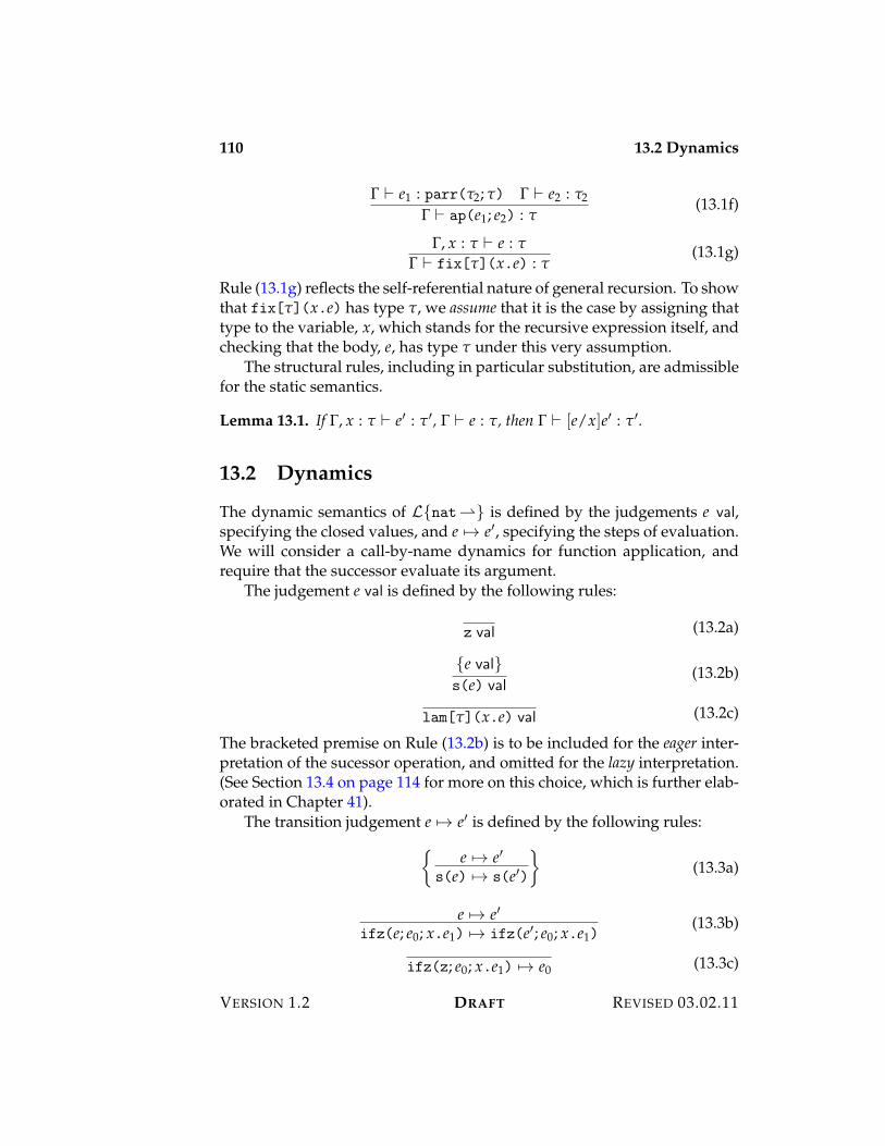
110 13.2 Dynamics
! ) e1 : parr("2; ") ! ) e2 : "2
! ) ap(e1; e2) : "(13.1f)
!, x : " ) e : "! ) fix["](x.e) : "
(13.1g)
Rule (13.1g) reflects the self-referential nature of general recursion. To showthat fix["](x.e) has type ", we assume that it is the case by assigning thattype to the variable, x, which stands for the recursive expression itself, andchecking that the body, e, has type " under this very assumption.
The structural rules, including in particular substitution, are admissiblefor the static semantics.
Lemma 13.1. If !, x : " ) e% : "%, ! ) e : ", then ! ) [e/x]e% : "%.
13.2 Dynamics
The dynamic semantics of L{nat"} is defined by the judgements e val,specifying the closed values, and e 53 e%, specifying the steps of evaluation.We will consider a call-by-name dynamics for function application, andrequire that the successor evaluate its argument.
The judgement e val is defined by the following rules:
z val (13.2a)
{e val}s(e) val
(13.2b)
lam["](x.e) val (13.2c)
The bracketed premise on Rule (13.2b) is to be included for the eager inter-pretation of the sucessor operation, and omitted for the lazy interpretation.(See Section 13.4 on page 114 for more on this choice, which is further elab-orated in Chapter 41).
The transition judgement e 53 e% is defined by the following rules:&
e 53 e%s(e) 53 s(e%)
'(13.3a)
e 53 e%ifz(e; e0; x.e1) 53 ifz(e%; e0; x.e1)
(13.3b)
ifz(z; e0; x.e1) 53 e0 (13.3c)
VERSION 1.2 DRAFT REVISED 03.02.11
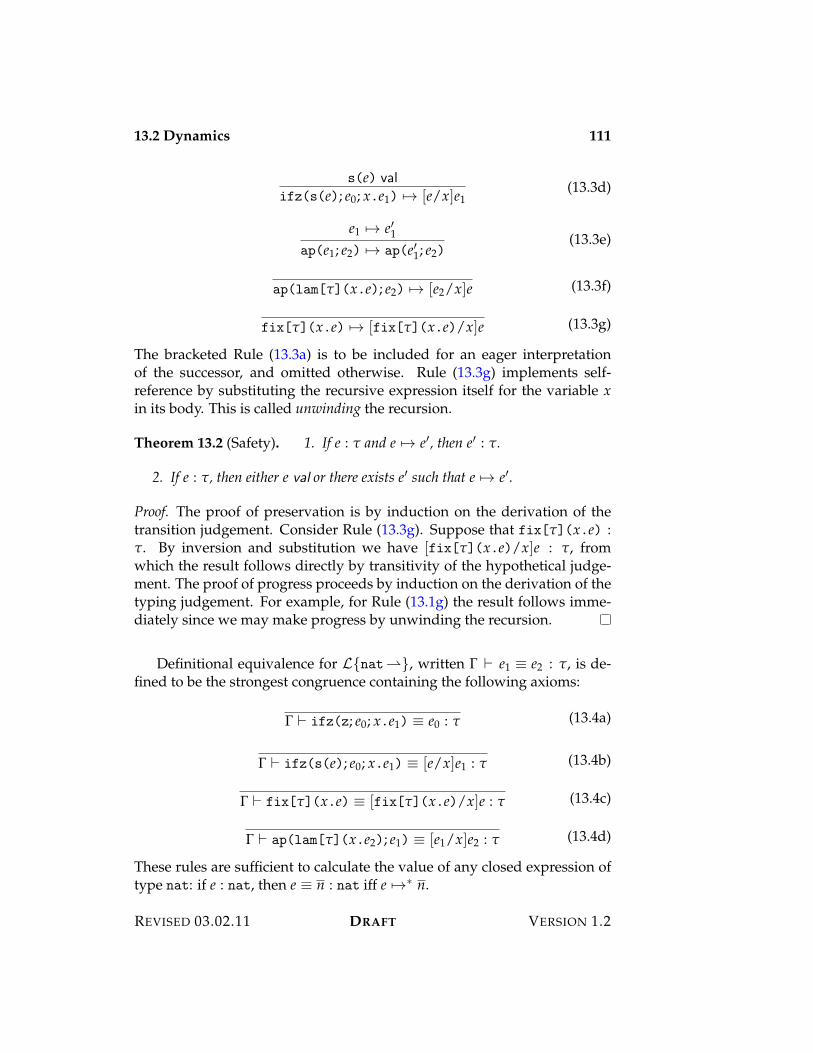
13.2 Dynamics 111
s(e) valifz(s(e); e0; x.e1) 53 [e/x]e1
(13.3d)
e1 53 e%1ap(e1; e2) 53 ap(e%1; e2)
(13.3e)
ap(lam["](x.e); e2) 53 [e2/x]e (13.3f)
fix["](x.e) 53 [fix["](x.e)/x]e (13.3g)
The bracketed Rule (13.3a) is to be included for an eager interpretationof the successor, and omitted otherwise. Rule (13.3g) implements self-reference by substituting the recursive expression itself for the variable xin its body. This is called unwinding the recursion.
Theorem 13.2 (Safety). 1. If e : " and e 53 e%, then e% : ".
2. If e : ", then either e val or there exists e% such that e 53 e%.
Proof. The proof of preservation is by induction on the derivation of thetransition judgement. Consider Rule (13.3g). Suppose that fix["](x.e) :". By inversion and substitution we have [fix["](x.e)/x]e : ", fromwhich the result follows directly by transitivity of the hypothetical judge-ment. The proof of progress proceeds by induction on the derivation of thetyping judgement. For example, for Rule (13.1g) the result follows imme-diately since we may make progress by unwinding the recursion.
Definitional equivalence for L{nat"}, written ! ) e1 9 e2 : ", is de-fined to be the strongest congruence containing the following axioms:
! ) ifz(z; e0; x.e1) 9 e0 : " (13.4a)
! ) ifz(s(e); e0; x.e1) 9 [e/x]e1 : " (13.4b)
! ) fix["](x.e) 9 [fix["](x.e)/x]e : " (13.4c)
! ) ap(lam["](x.e2); e1) 9 [e1/x]e2 : " (13.4d)
These rules are sufficient to calculate the value of any closed expression oftype nat: if e : nat, then e 9 n : nat iff e 531 n.
REVISED 03.02.11 DRAFT VERSION 1.2
112 13.3 Definability
13.3 Definability
General recursion is a very flexible programming technique that permits awide variety of functions to be defined within L{nat"}. The drawbackis that, in contrast to primitive recursion, the termination of a recursivelydefined function is not intrinsic to the program itself, but rather must beproved extrinsically by the programmer. The benefit is a much greater free-dom in writing programs.
General recursive functions are definable from general recursion andnon-recursive functions. Let us write fun x(y:"1):"2 is e for a recursivefunction within whose body, e : "2, are bound two variables, y : "1 stand-ing for the argument and x : "1 3 "2 standing for the function itself. Thedynamic semantics of this construct is given by the axiom
fun x(y:"1):"2 is e(e1) 53 [fun x(y:"1):"2 is e, e1/x, y]e.
That is, to apply a recursive function, we substitute the recursive functionitself for x and the argument for y in its body.
Recursive functions may be defined in L{nat"} using a combinationof recursion and functions, writing
fix x:"1 " "2 is! (y:"1. e)
for fun x(y:"1):"2 is e. It is a good exercise to check that the static anddynamic semantics of recursive functions are derivable from this definition.
The primitive recursion construct of L{nat3} is defined in L{nat"}using recursive functions by taking the expression
natrec e {z; e0 | s(x) with y ; e1}
to stand for the application, e%(e), where e% is the general recursive function
fun f(u:nat):" is ifz u {z; e0 | s(x); [ f(x)/y]e1}.
The static and dynamic semantics of primitive recursion are derivable inL{nat"} using this expansion.
In general, functions definable in L{nat"} are partial in that they maybe undefined for some arguments. A partial (mathematical) function, ' :N " N, is definable in L{nat"} iff there is an expression e' : nat" nat
such that '(m) = n iff e'(m) 9 n : nat. So, for example, if ' is the totallyundefined function, then e' is any function that loops without returningwhenever it is called.
VERSION 1.2 DRAFT REVISED 03.02.11
13.3 Definability 113
It is informative to classify those partial functions ' that are definablein L{nat"}. These are the so-called partial recursive functions, which aredefined to be the primitive recursive functions augmented by the minimiza-tion operation: given '(m, n), define ((n) to be the least m 7 0 such that(1) for m% < m, '(m%, n) is defined and non-zero, and (2) '(m, n) = 0. If nosuch m exists, then ((n) is undefined.
Theorem 13.3. A partial function ' on the natural numbers is definable in L{nat"}iff it is partial recursive.
Proof sketch. Minimization is readily definable in L{nat"}, so it is at leastas powerful as the set of partial recursive functions. Conversely, we may,with considerable tedium, define an evaluator for expressions of L{nat"}as a partial recursive function, using Godel-numbering to represent expres-sions as numbers. Consequently, L{nat"} does not exceed the power ofthe set of partial recursive functions.
Church’s Law states that the partial recursive functions coincide withthe set of effectively computable functions on the natural numbers—thosethat can be carried out by a program written in any programming languagecurrently available or that will ever be available.1 Therefore L{nat"} isas powerful as any other programming language with respect to the set ofdefinable functions on the natural numbers.
The universal function, 'univ, for L{nat"} is the partial function onthe natural numbers defined by
'univ("e#)(m) = n iff e(m) 9 n : nat.
In contrast to L{nat3}, the universal function 'univ for L{nat"} is par-tial (may be undefined for some inputs). It is, in essence, an interpreterthat, given the code "e# of a closed expression of type nat" nat, simulatesthe dynamic semantics to calculate the result, if any, of applying it to the m,obtaining n. Since this process may not terminate, the universal function isnot defined for all inputs.
By Church’s Law the universal function is definable in L{nat"}. Incontrast, we proved in Chapter 12 that the analogous function is not defin-able in L{nat3} using the technique of diagonalization. It is instructiveto examine why that argument does not apply in the present setting. As inSection 12.4 on page 104, we may derive the equivalence
eD("eD#) 9 s(eD("eD#))1See Chapter 20 for further discussion of Church’s Law.
REVISED 03.02.11 DRAFT VERSION 1.2
114 13.4 Co-Natural Numbers
for L{nat"}. The difference, however, is that this equation is not incon-sistent! Rather than being contradictory, it is merely a proof that the expres-sion eD("eD#) does not terminate when evaluated, for if it did, the resultwould be a number equal to its own successor, which is impossible.
13.4 Co-Natural Numbers
The dynamics of the successor operation on natural numbers may be takento be either eager or lazy, according to whether the predecessor of a suc-cessor is required to be a value. The eager interpretation represents thestandard natural numbers in the sense that if e : nat and e val, then e eval-uates to a numeral. The lazy interpretation, however, admits non-standard“natural numbers,” such as
) = fix x:nat is s(x).
The “number” ) evaluates to s()). This “number” may be thought of asan infinite stack of successors, since whenever we peel off the outermostsuccessor we obtain the same “number” back again. The “number” ) istherefore larger than any other natural number in the sense that one mayreach zero by repeatedly taking the predecessor of a natural number, butany number of predecessors on ) leads back to ) itself.
As the scare quotes indicate, it is stretching the terminology to refer to) as a natural number. Instead one should distinguish a new type, calledconat, of lazy natural numbers, of which ) is an element. The prefix “co-”indicates that the co-natural numbers are “dual” to the natural numbers inthe following sense. The natural numbers are inductively defined as theleast type such that if e 9 z : nat or e 9 s(e%) : nat for some e% : nat, thene : nat. Dually, the co-natural numbers may be regarded as the largest typesuch that if e : conat, then either e 9 z : conat, or e 9 s(e%) : nat for somee% : conat. The difference is that ) : conat, because ) is definitionallyequivalent to its own successor, whereas it is not the case that ) : nat,according to these definitions.
The duality between the natural numbers and the co-natural numbersis developed further in Chapter 18, wherein we consider the concepts ofinductive and co-inductive types. Eagerness and laziness in general is dis-cussed further in Chapter 41.
13.5 Exercises
VERSION 1.2 DRAFT REVISED 03.02.11
Part V
Finite Data Types

Chapter 14
Product Types
The binary product of two types consists of ordered pairs of values, one fromeach type in the order specified. The associated eliminatory forms are pro-jections, which select the first and second component of a pair. The nullaryproduct, or unit, type consists solely of the unique “null tuple” of no val-ues, and has no associated eliminatory form. The product type admits botha lazy and an eager dynamics. According to the lazy dynamics, a pair isa value without regard to whether its components are values; they are notevaluated until (if ever) they are accessed and used in another computation.According to the eager dynamics, a pair is a value only if its componentsare values; they are evaluated when the pair is created.
More generally, we may consider the finite product, &i+I "i, indexed bya finite set of indices, I. The elements of the finite product type are I-indexedtuples whose ith component is an element of the type "i, for each i + I.The components are accessed by I-indexed projection operations, generaliz-ing the binary case. Special cases of the finite product include n-tuples, in-dexed by sets of the form I = { 0, . . . , n $ 1 }, and labelled tuples, or records,indexed by finite sets of symbols. Similarly to binary products, finite prod-ucts admit both an eager and a lazy interpretation.
118 14.1 Nullary and Binary Products
14.1 Nullary and Binary Products
The abstract syntax of products is given by the following grammar:
Type " ::= unit unit nullary productprod("1; "2) "1 < "2 binary product
Expr e ::= triv ?@ null tuplepair(e1; e2) ?e1, e2@ ordered pairproj[l](e) e · l left projectionproj[r](e) e · r right projection
There is no elimination form for the unit type, there being nothing to extractfrom the null tuple.
The statics of product types is given by the following rules.
! ) triv : unit(14.1a)
! ) e1 : "1 ! ) e2 : "2! ) pair(e1; e2) : prod("1; "2)
(14.1b)
! ) e : prod("1; "2)
! ) proj[l](e) : "1(14.1c)
! ) e : prod("1; "2)
! ) proj[r](e) : "2(14.1d)
The dynamics of product types is specified by the following rules:
triv val(14.2a)
{e1 val} {e2 val}pair(e1; e2) val
(14.2b)
& e1 53 e%1pair(e1; e2) 53 pair(e%1; e2)
'(14.2c)
& e1 val e2 53 e%2pair(e1; e2) 53 pair(e1; e%2)
'(14.2d)
e 53 e%proj[l](e) 53 proj[l](e%) (14.2e)
e 53 e%proj[r](e) 53 proj[r](e%) (14.2f)
VERSION 1.2 DRAFT REVISED 03.02.11
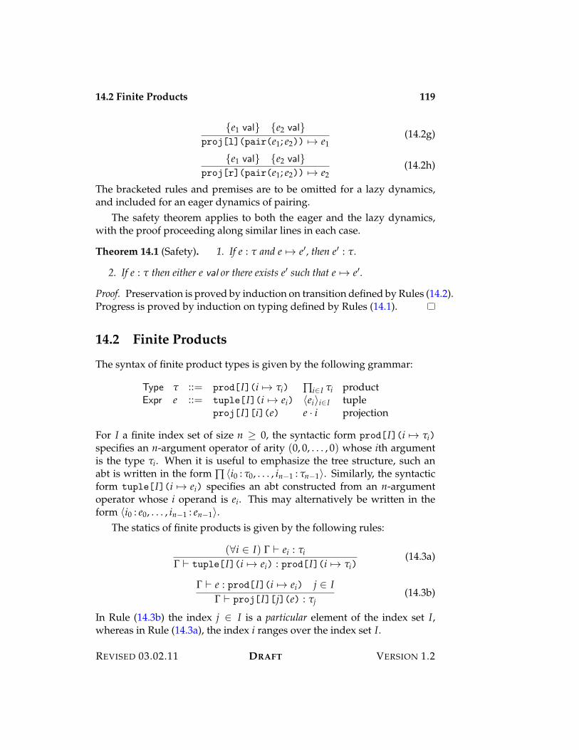
14.2 Finite Products 119
{e1 val} {e2 val}proj[l](pair(e1; e2)) 53 e1
(14.2g)
{e1 val} {e2 val}proj[r](pair(e1; e2)) 53 e2
(14.2h)
The bracketed rules and premises are to be omitted for a lazy dynamics,and included for an eager dynamics of pairing.
The safety theorem applies to both the eager and the lazy dynamics,with the proof proceeding along similar lines in each case.
Theorem 14.1 (Safety). 1. If e : " and e 53 e%, then e% : ".
2. If e : " then either e val or there exists e% such that e 53 e%.
Proof. Preservation is proved by induction on transition defined by Rules (14.2).Progress is proved by induction on typing defined by Rules (14.1).
14.2 Finite Products
The syntax of finite product types is given by the following grammar:
Type " ::= prod[I](i 53 "i) &i+I "i productExpr e ::= tuple[I](i 53 ei) ?ei@i+I tuple
proj[I][i](e) e · i projection
For I a finite index set of size n 7 0, the syntactic form prod[I](i 53 "i)
specifies an n-argument operator of arity (0, 0, . . . , 0) whose ith argumentis the type "i. When it is useful to emphasize the tree structure, such anabt is written in the form & ?i0 : "0, . . . , in$1 : "n$1@. Similarly, the syntacticform tuple[I](i 53 ei) specifies an abt constructed from an n-argumentoperator whose i operand is ei. This may alternatively be written in theform ?i0 : e0, . . . , in$1 : en$1@.
The statics of finite products is given by the following rules:
(&i + I) ! ) ei : "i
! ) tuple[I](i 53 ei) : prod[I](i 53 "i)(14.3a)
! ) e : prod[I](i 53 ei) j + I! ) proj[I][j](e) : "j
(14.3b)
In Rule (14.3b) the index j + I is a particular element of the index set I,whereas in Rule (14.3a), the index i ranges over the index set I.
REVISED 03.02.11 DRAFT VERSION 1.2
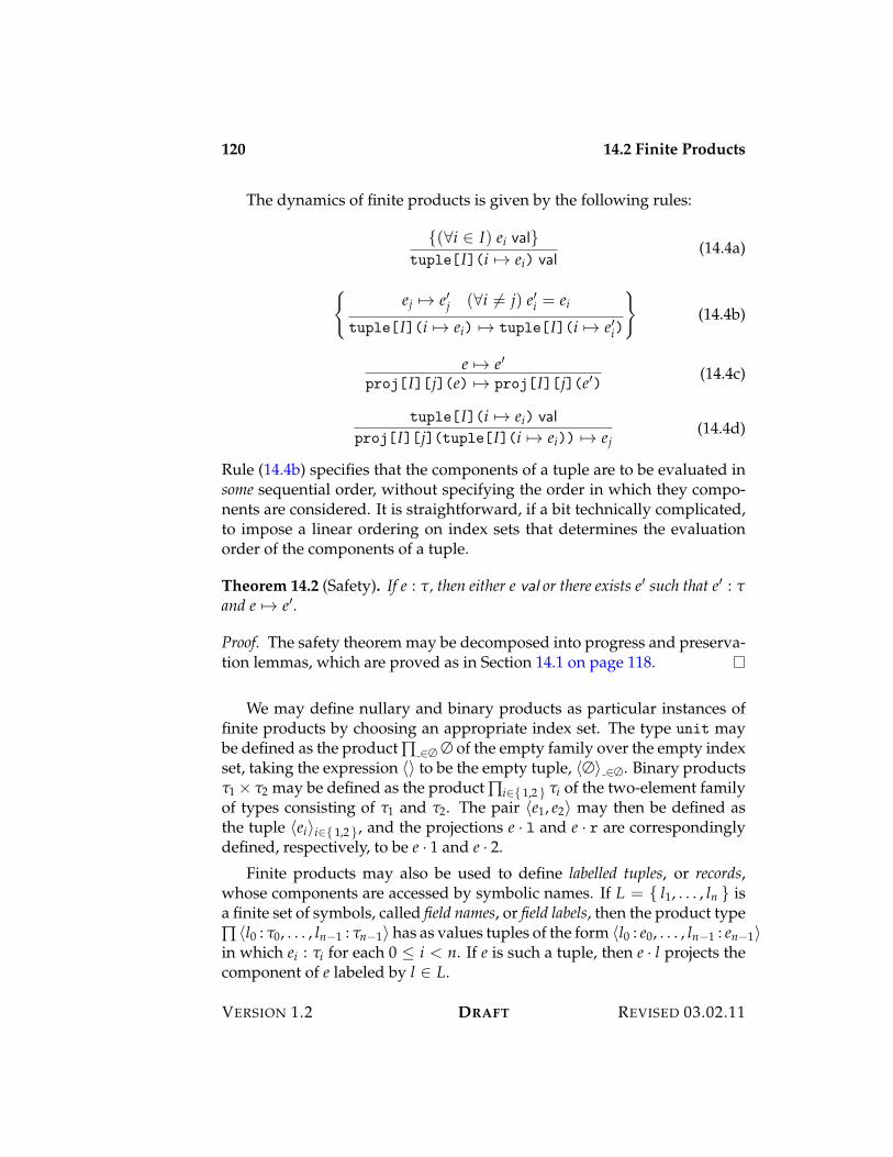
120 14.2 Finite Products
The dynamics of finite products is given by the following rules:
{(&i + I) ei val}tuple[I](i 53 ei) val
(14.4a)
%ej 53 e%j (&i ,= j) e%i = ei
tuple[I](i 53 ei) 53 tuple[I](i 53 e%i)
((14.4b)
e 53 e%proj[I][j](e) 53 proj[I][j](e%) (14.4c)
tuple[I](i 53 ei) valproj[I][j](tuple[I](i 53 ei)) 53 ej
(14.4d)
Rule (14.4b) specifies that the components of a tuple are to be evaluated insome sequential order, without specifying the order in which they compo-nents are considered. It is straightforward, if a bit technically complicated,to impose a linear ordering on index sets that determines the evaluationorder of the components of a tuple.
Theorem 14.2 (Safety). If e : ", then either e val or there exists e% such that e% : "and e 53 e%.
Proof. The safety theorem may be decomposed into progress and preserva-tion lemmas, which are proved as in Section 14.1 on page 118.
We may define nullary and binary products as particular instances offinite products by choosing an appropriate index set. The type unit maybe defined as the product & +# # of the empty family over the empty indexset, taking the expression ?@ to be the empty tuple, ?#@ +#. Binary products"1 < "2 may be defined as the product &i+{ 1,2 } "i of the two-element familyof types consisting of "1 and "2. The pair ?e1, e2@ may then be defined asthe tuple ?ei@i+{ 1,2 }, and the projections e · l and e · r are correspondinglydefined, respectively, to be e · 1 and e · 2.
Finite products may also be used to define labelled tuples, or records,whose components are accessed by symbolic names. If L = { l1, . . . , ln } isa finite set of symbols, called field names, or field labels, then the product type& ?l0 : "0, . . . , ln$1 : "n$1@ has as values tuples of the form ?l0 : e0, . . . , ln$1 : en$1@in which ei : "i for each 0 ( i < n. If e is such a tuple, then e · l projects thecomponent of e labeled by l + L.
VERSION 1.2 DRAFT REVISED 03.02.11
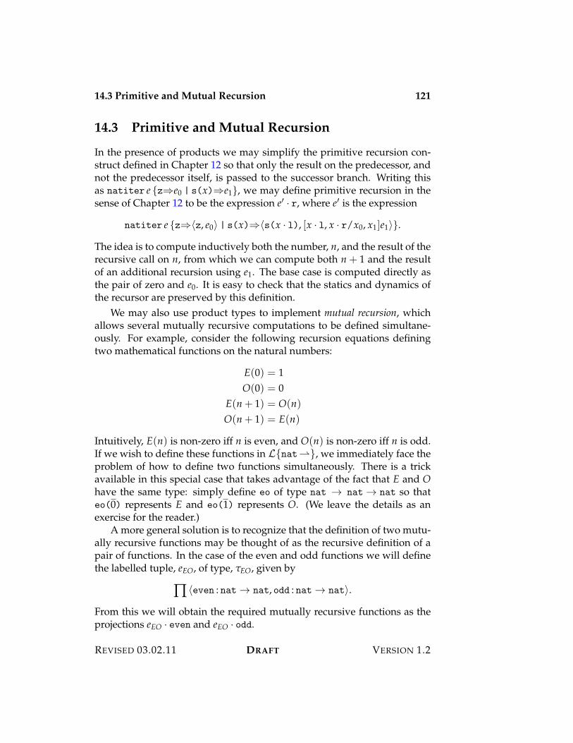
14.3 Primitive and Mutual Recursion 121
14.3 Primitive and Mutual Recursion
In the presence of products we may simplify the primitive recursion con-struct defined in Chapter 12 so that only the result on the predecessor, andnot the predecessor itself, is passed to the successor branch. Writing thisas natiter e {z;e0 | s(x);e1}, we may define primitive recursion in thesense of Chapter 12 to be the expression e% · r, where e% is the expression
natiter e {z;?z, e0@ | s(x);?s(x · l), [x · l, x · r/x0, x1]e1@}.
The idea is to compute inductively both the number, n, and the result of therecursive call on n, from which we can compute both n + 1 and the resultof an additional recursion using e1. The base case is computed directly asthe pair of zero and e0. It is easy to check that the statics and dynamics ofthe recursor are preserved by this definition.
We may also use product types to implement mutual recursion, whichallows several mutually recursive computations to be defined simultane-ously. For example, consider the following recursion equations definingtwo mathematical functions on the natural numbers:
E(0) = 1O(0) = 0
E(n + 1) = O(n)O(n + 1) = E(n)
Intuitively, E(n) is non-zero iff n is even, and O(n) is non-zero iff n is odd.If we wish to define these functions in L{nat"}, we immediately face theproblem of how to define two functions simultaneously. There is a trickavailable in this special case that takes advantage of the fact that E and Ohave the same type: simply define eo of type nat 3 nat 3 nat so thateo(0) represents E and eo(1) represents O. (We leave the details as anexercise for the reader.)
A more general solution is to recognize that the definition of two mutu-ally recursive functions may be thought of as the recursive definition of apair of functions. In the case of the even and odd functions we will definethe labelled tuple, eEO, of type, "EO, given by
& ?even : nat 3 nat, odd : nat 3 nat@.
From this we will obtain the required mutually recursive functions as theprojections eEO · even and eEO · odd.
REVISED 03.02.11 DRAFT VERSION 1.2
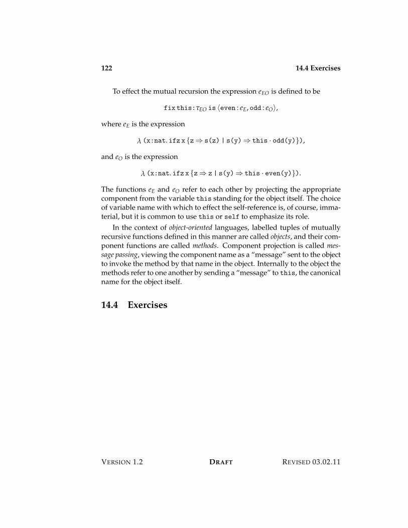
122 14.4 Exercises
To effect the mutual recursion the expression eEO is defined to be
fix this:"EO is ?even : eE, odd : eO@,
where eE is the expression
! (x:nat. ifz x {z; s(z) | s(y); this · odd(y)}),
and eO is the expression
! (x:nat. ifz x {z; z | s(y); this · even(y)}).
The functions eE and eO refer to each other by projecting the appropriatecomponent from the variable this standing for the object itself. The choiceof variable name with which to effect the self-reference is, of course, imma-terial, but it is common to use this or self to emphasize its role.
In the context of object-oriented languages, labelled tuples of mutuallyrecursive functions defined in this manner are called objects, and their com-ponent functions are called methods. Component projection is called mes-sage passing, viewing the component name as a “message” sent to the objectto invoke the method by that name in the object. Internally to the object themethods refer to one another by sending a “message” to this, the canonicalname for the object itself.
14.4 Exercises
VERSION 1.2 DRAFT REVISED 03.02.11
Chapter 15
Sum Types
Most data structures involve alternatives such as the distinction between aleaf and an interior node in a tree, or a choice in the outermost form of apiece of abstract syntax. Importantly, the choice determines the structureof the value. For example, nodes have children, but leaves do not, and soforth. These concepts are expressed by sum types, specifically the binarysum, which offers a choice of two things, and the nullary sum, which offersa choice of no things. Finite sums generalize nullary and binary sums topermit an arbitrary number of cases indexed by a finite index set. As withproducts, sums come in both eager and lazy variants, differing in how val-ues of sum type are defined.
15.1 Binary and Nullary Sums
The abstract syntax of sums is given by the following grammar:
Type " ::= void void nullary sumsum("1; "2) "1 + "2 binary sum
Expr e ::= abort["](e) abort" e abortin[l]["](e) l · e left injectionin[r]["](e) r · e right injectioncase(e; x1.e1; x2.e2) case e {l · x1 ; e1 | r · x2 ; e2} case analysis
The nullary sum represents a choice of zero alternatives, and hence ad-mits no introductory form. The eliminatory form, abort["](e), abortsthe computation in the event that e evaluates to a value, which it cannotdo. The elements of the binary sum type are labelled to indicate whether
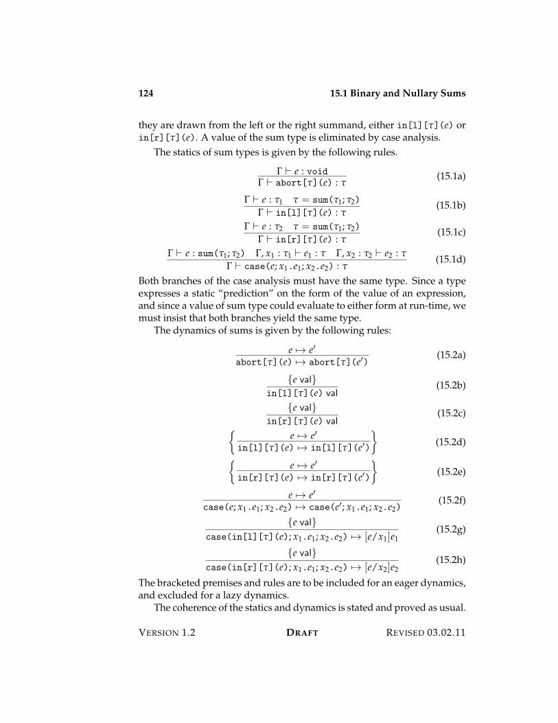
124 15.1 Binary and Nullary Sums
they are drawn from the left or the right summand, either in[l]["](e) orin[r]["](e). A value of the sum type is eliminated by case analysis.
The statics of sum types is given by the following rules.
! ) e : void! ) abort["](e) : "
(15.1a)
! ) e : "1 " = sum("1; "2)
! ) in[l]["](e) : "(15.1b)
! ) e : "2 " = sum("1; "2)
! ) in[r]["](e) : "(15.1c)
! ) e : sum("1; "2) !, x1 : "1 ) e1 : " !, x2 : "2 ) e2 : "! ) case(e; x1.e1; x2.e2) : "
(15.1d)
Both branches of the case analysis must have the same type. Since a typeexpresses a static “prediction” on the form of the value of an expression,and since a value of sum type could evaluate to either form at run-time, wemust insist that both branches yield the same type.
The dynamics of sums is given by the following rules:
e 53 e%abort["](e) 53 abort["](e%)
(15.2a)
{e val}in[l]["](e) val
(15.2b)
{e val}in[r]["](e) val
(15.2c)&
e 53 e%in[l]["](e) 53 in[l]["](e%)
'(15.2d)
&e 53 e%
in[r]["](e) 53 in[r]["](e%)
'(15.2e)
e 53 e%case(e; x1.e1; x2.e2) 53 case(e%; x1.e1; x2.e2)
(15.2f)
{e val}case(in[l]["](e); x1.e1; x2.e2) 53 [e/x1]e1
(15.2g)
{e val}case(in[r]["](e); x1.e1; x2.e2) 53 [e/x2]e2
(15.2h)
The bracketed premises and rules are to be included for an eager dynamics,and excluded for a lazy dynamics.
The coherence of the statics and dynamics is stated and proved as usual.
VERSION 1.2 DRAFT REVISED 03.02.11
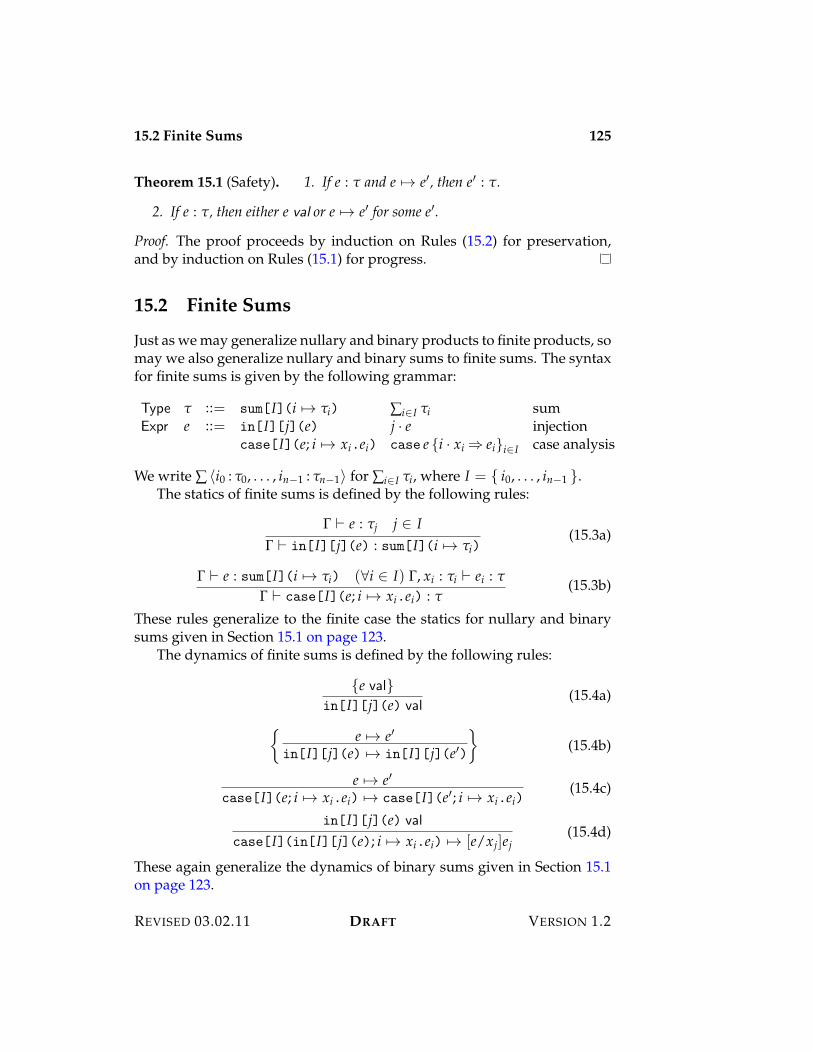
15.2 Finite Sums 125
Theorem 15.1 (Safety). 1. If e : " and e 53 e%, then e% : ".
2. If e : ", then either e val or e 53 e% for some e%.
Proof. The proof proceeds by induction on Rules (15.2) for preservation,and by induction on Rules (15.1) for progress.
15.2 Finite Sums
Just as we may generalize nullary and binary products to finite products, somay we also generalize nullary and binary sums to finite sums. The syntaxfor finite sums is given by the following grammar:
Type " ::= sum[I](i 53 "i) 'i+I "i sumExpr e ::= in[I][j](e) j · e injection
case[I](e; i 53 xi.ei) case e {i · xi ; ei}i+I case analysis
We write ' ?i0 : "0, . . . , in$1 : "n$1@ for 'i+I "i, where I = { i0, . . . , in$1 }.The statics of finite sums is defined by the following rules:
! ) e : "j j + I! ) in[I][j](e) : sum[I](i 53 "i)
(15.3a)
! ) e : sum[I](i 53 "i) (&i + I) !, xi : "i ) ei : "
! ) case[I](e; i 53 xi.ei) : "(15.3b)
These rules generalize to the finite case the statics for nullary and binarysums given in Section 15.1 on page 123.
The dynamics of finite sums is defined by the following rules:
{e val}in[I][j](e) val
(15.4a)
&e 53 e%
in[I][j](e) 53 in[I][j](e%)
'(15.4b)
e 53 e%case[I](e; i 53 xi.ei) 53 case[I](e%; i 53 xi.ei)
(15.4c)
in[I][j](e) val
case[I](in[I][j](e); i 53 xi.ei) 53 [e/xj]ej(15.4d)
These again generalize the dynamics of binary sums given in Section 15.1on page 123.
REVISED 03.02.11 DRAFT VERSION 1.2
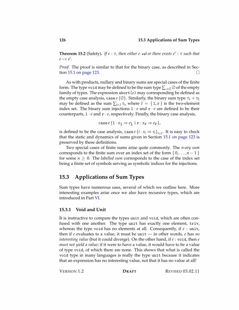
126 15.3 Applications of Sum Types
Theorem 15.2 (Safety). If e : ", then either e val or there exists e% : " such thate 53 e%.
Proof. The proof is similar to that for the binary case, as described in Sec-tion 15.1 on page 123.
As with products, nullary and binary sums are special cases of the finiteform. The type voidmay be defined to be the sum type ' +# # of the emptyfamily of types. The expression abort(e) may corresponding be defined asthe empty case analysis, case e {#}. Similarly, the binary sum type "1 + "2may be defined as the sum 'i+I "i, where I = { l, r } is the two-elementindex set. The binary sum injections l · e and r · e are defined to be theircounterparts, l · e and r · e, respectively. Finally, the binary case analysis,
case e {l · xl; el | r · xr; er},
is defined to be the case analysis, case e {i · xi ; "i}i+I . It is easy to checkthat the static and dynamics of sums given in Section 15.1 on page 123 ispreserved by these definitions.
Two special cases of finite sums arise quite commonly. The n-ary sumcorresponds to the finite sum over an index set of the form { 0, . . . , n $ 1 }for some n 7 0. The labelled sum corresponds to the case of the index setbeing a finite set of symbols serving as symbolic indices for the injections.
15.3 Applications of Sum Types
Sum types have numerous uses, several of which we outline here. Moreinteresting examples arise once we also have recursive types, which areintroduced in Part VI.
15.3.1 Void and Unit
It is instructive to compare the types unit and void, which are often con-fused with one another. The type unit has exactly one element, triv,whereas the type void has no elements at all. Consequently, if e : unit,then if e evaluates to a value, it must be unit — in other words, e has nointeresting value (but it could diverge). On the other hand, if e : void, then emust not yield a value; if it were to have a value, it would have to be a valueof type void, of which there are none. This shows that what is called thevoid type in many languages is really the type unit because it indicatesthat an expression has no interesting value, not that it has no value at all!
VERSION 1.2 DRAFT REVISED 03.02.11
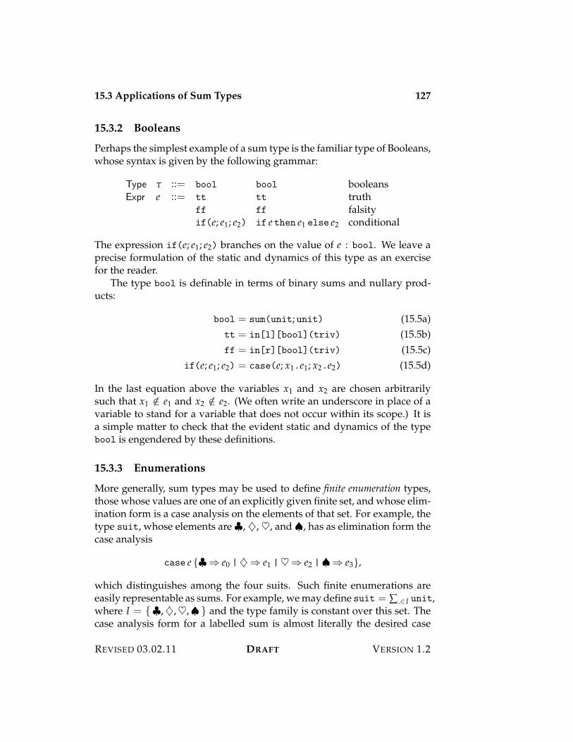
15.3 Applications of Sum Types 127
15.3.2 Booleans
Perhaps the simplest example of a sum type is the familiar type of Booleans,whose syntax is given by the following grammar:
Type " ::= bool bool booleansExpr e ::= tt tt truth
ff ff falsityif(e; e1; e2) if e then e1 else e2 conditional
The expression if(e; e1; e2) branches on the value of e : bool. We leave aprecise formulation of the static and dynamics of this type as an exercisefor the reader.
The type bool is definable in terms of binary sums and nullary prod-ucts:
bool = sum(unit; unit) (15.5a)tt = in[l][bool](triv) (15.5b)ff = in[r][bool](triv) (15.5c)
if(e; e1; e2) = case(e; x1.e1; x2.e2) (15.5d)
In the last equation above the variables x1 and x2 are chosen arbitrarilysuch that x1 /+ e1 and x2 /+ e2. (We often write an underscore in place of avariable to stand for a variable that does not occur within its scope.) It isa simple matter to check that the evident static and dynamics of the typebool is engendered by these definitions.
15.3.3 Enumerations
More generally, sum types may be used to define finite enumeration types,those whose values are one of an explicitly given finite set, and whose elim-ination form is a case analysis on the elements of that set. For example, thetype suit, whose elements are A, B, C, and D, has as elimination form thecase analysis
case e {A; e0 |B; e1 |C; e2 |D; e3},
which distinguishes among the four suits. Such finite enumerations areeasily representable as sums. For example, we may define suit = ' +I unit,where I = {A,B,C,D } and the type family is constant over this set. Thecase analysis form for a labelled sum is almost literally the desired case
REVISED 03.02.11 DRAFT VERSION 1.2
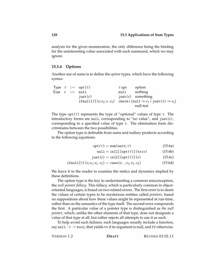
128 15.3 Applications of Sum Types
analysis for the given enumeration, the only difference being the bindingfor the uninteresting value associated with each summand, which we mayignore.
15.3.4 Options
Another use of sums is to define the option types, which have the followingsyntax:
Type " ::= opt(") " opt optionExpr e ::= null null nothing
just(e) just(e) somethingifnull["](e; e1; x.e2) check e {null; e1 | just(x); e2}
null test
The type opt(") represents the type of “optional” values of type ". Theintroductory forms are null, corresponding to “no value”, and just(e),corresponding to a specified value of type ". The elimination form dis-criminates between the two possibilities.
The option type is definable from sums and nullary products accordingto the following equations:
opt(") = sum(unit; ") (15.6a)null = in[l][opt(")](triv) (15.6b)
just(e) = in[r][opt(")](e) (15.6c)ifnull["](e; e1; x2.e2) = case(e; .e1; x2.e2) (15.6d)
We leave it to the reader to examine the statics and dynamics implied bythese definitions.
The option type is the key to understanding a common misconception,the null pointer fallacy. This fallacy, which is particularly common in object-oriented languages, is based on two related errors. The first error is to deemthe values of certain types to be mysterious entities called pointers, basedon suppositions about how these values might be represented at run-time,rather than on the semantics of the type itself. The second error compoundsthe first. A particular value of a pointer type is distinguished as the nullpointer, which, unlike the other elements of that type, does not designate avalue of that type at all, but rather rejects all attempts to use it as such.
To help avoid such failures, such languages usually include a function,say null : " 3 bool, that yields tt if its argument is null, and ff otherwise.
VERSION 1.2 DRAFT REVISED 03.02.11
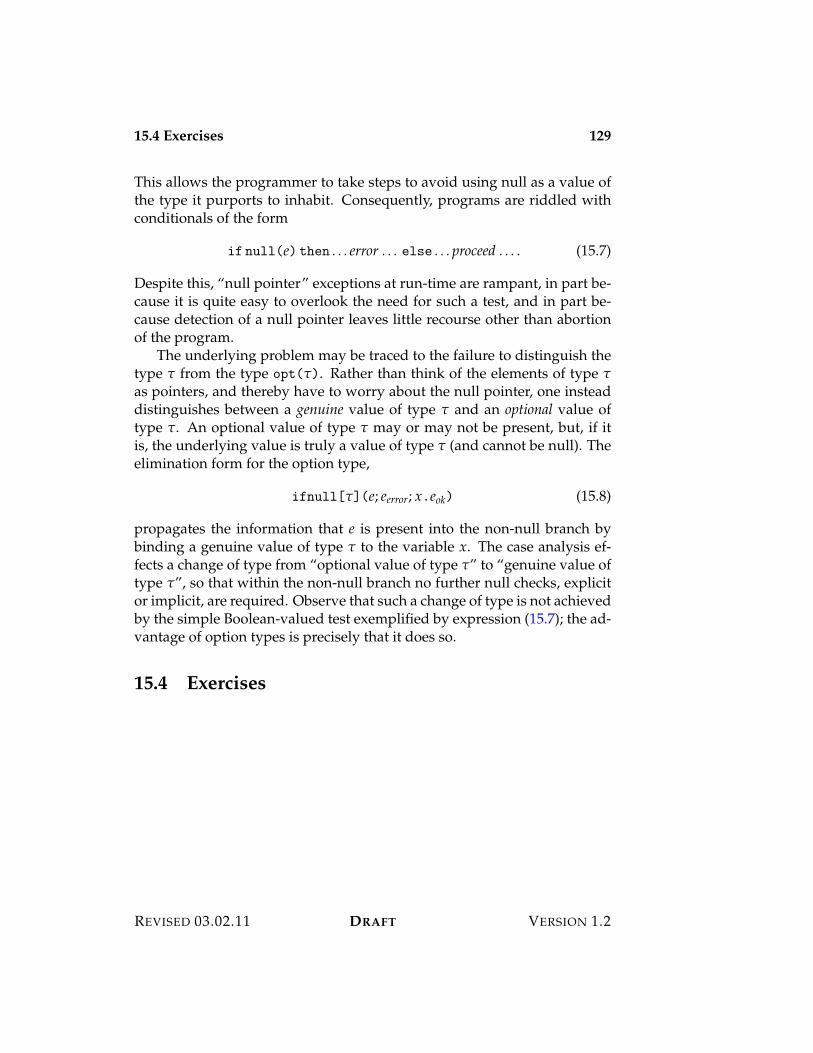
15.4 Exercises 129
This allows the programmer to take steps to avoid using null as a value ofthe type it purports to inhabit. Consequently, programs are riddled withconditionals of the form
if null(e) then . . . error . . . else . . . proceed . . . . (15.7)
Despite this, “null pointer” exceptions at run-time are rampant, in part be-cause it is quite easy to overlook the need for such a test, and in part be-cause detection of a null pointer leaves little recourse other than abortionof the program.
The underlying problem may be traced to the failure to distinguish thetype " from the type opt("). Rather than think of the elements of type "as pointers, and thereby have to worry about the null pointer, one insteaddistinguishes between a genuine value of type " and an optional value oftype ". An optional value of type " may or may not be present, but, if itis, the underlying value is truly a value of type " (and cannot be null). Theelimination form for the option type,
ifnull["](e; eerror; x.eok) (15.8)
propagates the information that e is present into the non-null branch bybinding a genuine value of type " to the variable x. The case analysis ef-fects a change of type from “optional value of type "” to “genuine value oftype "”, so that within the non-null branch no further null checks, explicitor implicit, are required. Observe that such a change of type is not achievedby the simple Boolean-valued test exemplified by expression (15.7); the ad-vantage of option types is precisely that it does so.
15.4 Exercises
REVISED 03.02.11 DRAFT VERSION 1.2

130 15.4 Exercises
VERSION 1.2 DRAFT REVISED 03.02.11
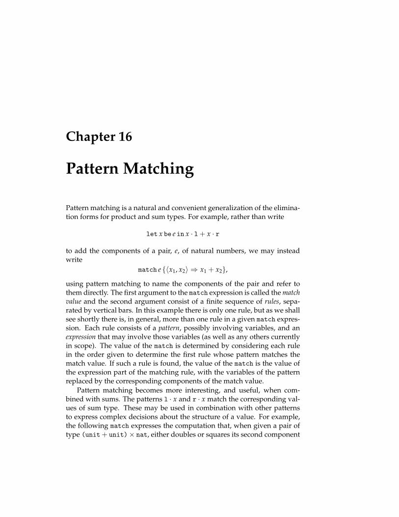
Chapter 16
Pattern Matching
Pattern matching is a natural and convenient generalization of the elimina-tion forms for product and sum types. For example, rather than write
let x be e in x · l+ x · r
to add the components of a pair, e, of natural numbers, we may insteadwrite
match e {?x1, x2@ ; x1 + x2},
using pattern matching to name the components of the pair and refer tothem directly. The first argument to the match expression is called the matchvalue and the second argument consist of a finite sequence of rules, sepa-rated by vertical bars. In this example there is only one rule, but as we shallsee shortly there is, in general, more than one rule in a given match expres-sion. Each rule consists of a pattern, possibly involving variables, and anexpression that may involve those variables (as well as any others currentlyin scope). The value of the match is determined by considering each rulein the order given to determine the first rule whose pattern matches thematch value. If such a rule is found, the value of the match is the value ofthe expression part of the matching rule, with the variables of the patternreplaced by the corresponding components of the match value.
Pattern matching becomes more interesting, and useful, when com-bined with sums. The patterns l · x and r · x match the corresponding val-ues of sum type. These may be used in combination with other patternsto express complex decisions about the structure of a value. For example,the following match expresses the computation that, when given a pair oftype (unit+ unit)< nat, either doubles or squares its second component
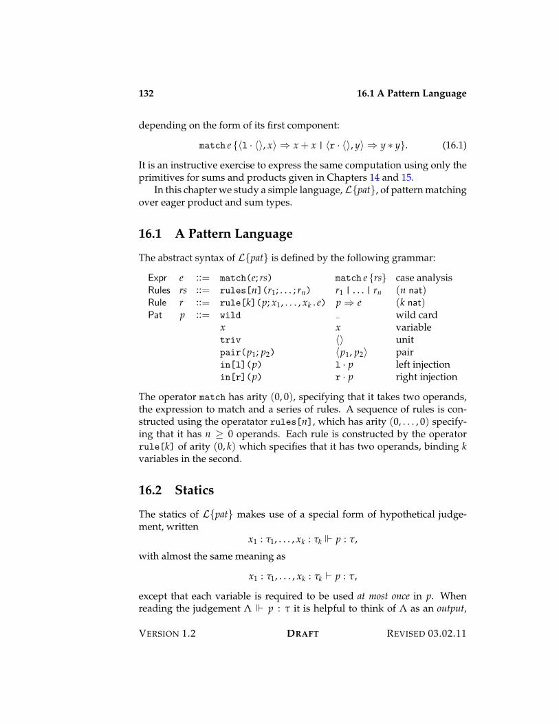
132 16.1 A Pattern Language
depending on the form of its first component:
match e {?l · ?@, x@ ; x + x | ?r · ?@, y@ ; y 1 y}. (16.1)
It is an instructive exercise to express the same computation using only theprimitives for sums and products given in Chapters 14 and 15.
In this chapter we study a simple language, L{pat}, of pattern matchingover eager product and sum types.
16.1 A Pattern Language
The abstract syntax of L{pat} is defined by the following grammar:
Expr e ::= match(e; rs) match e {rs} case analysisRules rs ::= rules[n](r1; . . . ; rn) r1 | . . . | rn (n nat)Rule r ::= rule[k](p; x1, . . . , xk.e) p ; e (k nat)Pat p ::= wild wild card
x x variabletriv ?@ unitpair(p1; p2) ?p1, p2@ pairin[l](p) l · p left injectionin[r](p) r · p right injection
The operator match has arity (0, 0), specifying that it takes two operands,the expression to match and a series of rules. A sequence of rules is con-structed using the operatator rules[n], which has arity (0, . . . , 0) specify-ing that it has n 7 0 operands. Each rule is constructed by the operatorrule[k] of arity (0, k) which specifies that it has two operands, binding kvariables in the second.
16.2 Statics
The statics of L{pat} makes use of a special form of hypothetical judge-ment, written
x1 : "1, . . . , xk : "k $ p : ",
with almost the same meaning as
x1 : "1, . . . , xk : "k ) p : ",
except that each variable is required to be used at most once in p. Whenreading the judgement ( $ p : " it is helpful to think of ( as an output,
VERSION 1.2 DRAFT REVISED 03.02.11
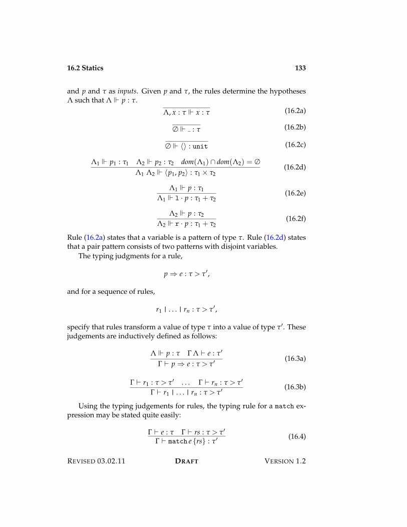
16.2 Statics 133
and p and " as inputs. Given p and ", the rules determine the hypotheses( such that ( $ p : ".
(, x : " $ x : " (16.2a)
# $ : " (16.2b)
# $ ?@ : unit (16.2c)
(1 $ p1 : "1 (2 $ p2 : "2 dom((1) 0 dom((2) = #(1 (2 $ ?p1, p2@ : "1 < "2
(16.2d)
(1 $ p : "1
(1 $ l · p : "1 + "2(16.2e)
(2 $ p : "2
(2 $ r · p : "1 + "2(16.2f)
Rule (16.2a) states that a variable is a pattern of type ". Rule (16.2d) statesthat a pair pattern consists of two patterns with disjoint variables.
The typing judgments for a rule,
p ; e : " > "%,
and for a sequence of rules,
r1 | . . . | rn : " > "%,
specify that rules transform a value of type " into a value of type "%. Thesejudgements are inductively defined as follows:
( $ p : " ! ( ) e : "%
! ) p ; e : " > "% (16.3a)
! ) r1 : " > "% . . . ! ) rn : " > "%
! ) r1 | . . . | rn : " > "% (16.3b)
Using the typing judgements for rules, the typing rule for a match ex-pression may be stated quite easily:
! ) e : " ! ) rs : " > "%
! ) match e {rs} : "% (16.4)
REVISED 03.02.11 DRAFT VERSION 1.2
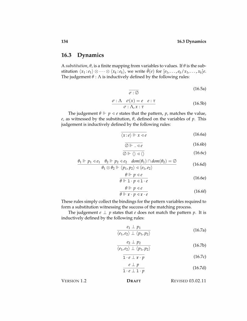
134 16.3 Dynamics
16.3 Dynamics
A substitution, *, is a finite mapping from variables to values. If * is the sub-stitution ?x1 : e1@ E · · · E ?xk : ek@, we write *(e) for [e1, . . . , ek/x1, . . . , xk]e.The judgement * : ( is inductively defined by the following rules:
& : #(16.5a)
& : ( &(x) = e e : "
& : (, x : "(16.5b)
The judgement * $ p # e states that the pattern, p, matches the value,e, as witnessed by the substitution, *, defined on the variables of p. Thisjudgement is inductively defined by the following rules:
?x : e@ $ x # e (16.6a)
# $ # e (16.6b)
# $ ?@ # ?@ (16.6c)
*1 $ p1 # e1 *2 $ p2 # e2 dom(*1) 0 dom(*2) = #*1 E *2 $ ?p1, p2@ # ?e1, e2@
(16.6d)
* $ p # e* $ l · p # l · e
(16.6e)
* $ p # e* $ r · p # r · e
(16.6f)
These rules simply collect the bindings for the pattern variables required toform a substitution witnessing the success of the matching process.
The judgement e > p states that e does not match the pattern p. It isinductively defined by the following rules:
e1 > p1
?e1, e2@ > ?p1, p2@(16.7a)
e2 > p2
?e1, e2@ > ?p1, p2@(16.7b)
l · e > r · p (16.7c)
e > pl · e > l · p
(16.7d)
VERSION 1.2 DRAFT REVISED 03.02.11
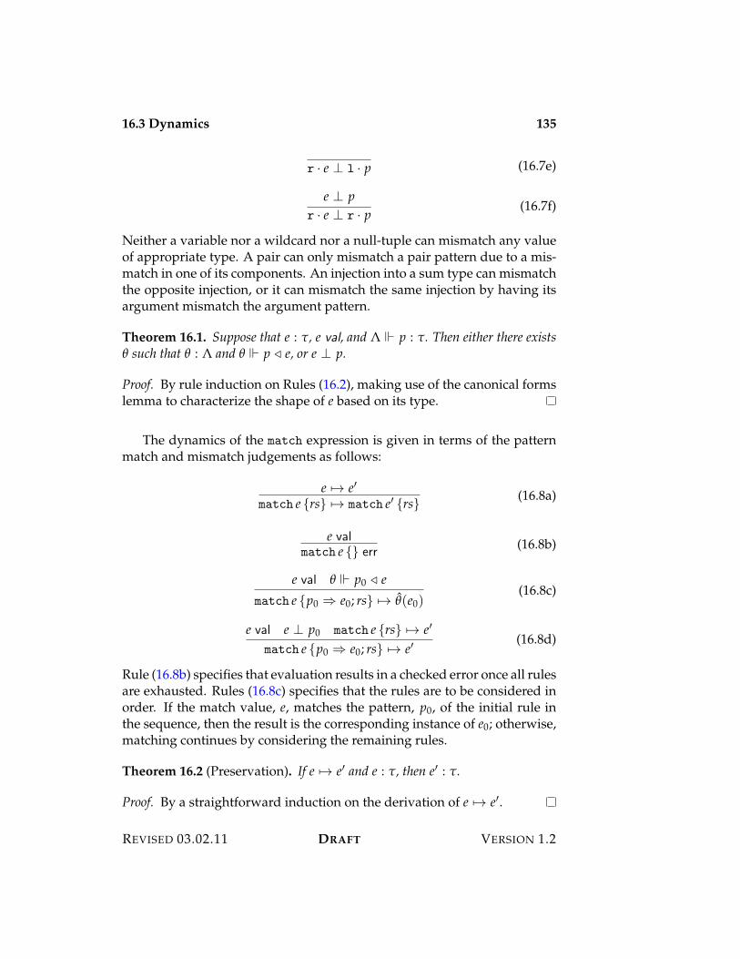
16.3 Dynamics 135
r · e > l · p (16.7e)
e > pr · e > r · p
(16.7f)
Neither a variable nor a wildcard nor a null-tuple can mismatch any valueof appropriate type. A pair can only mismatch a pair pattern due to a mis-match in one of its components. An injection into a sum type can mismatchthe opposite injection, or it can mismatch the same injection by having itsargument mismatch the argument pattern.
Theorem 16.1. Suppose that e : ", e val, and ( $ p : ". Then either there exists* such that * : ( and * $ p # e, or e > p.
Proof. By rule induction on Rules (16.2), making use of the canonical formslemma to characterize the shape of e based on its type.
The dynamics of the match expression is given in terms of the patternmatch and mismatch judgements as follows:
e 53 e%match e {rs} 53 match e% {rs} (16.8a)
e valmatch e {} err
(16.8b)
e val * $ p0 # ematch e {p0 ; e0; rs} 53 *(e0)
(16.8c)
e val e > p0 match e {rs} 53 e%
match e {p0 ; e0; rs} 53 e%(16.8d)
Rule (16.8b) specifies that evaluation results in a checked error once all rulesare exhausted. Rules (16.8c) specifies that the rules are to be considered inorder. If the match value, e, matches the pattern, p0, of the initial rule inthe sequence, then the result is the corresponding instance of e0; otherwise,matching continues by considering the remaining rules.
Theorem 16.2 (Preservation). If e 53 e% and e : ", then e% : ".
Proof. By a straightforward induction on the derivation of e 53 e%.
REVISED 03.02.11 DRAFT VERSION 1.2
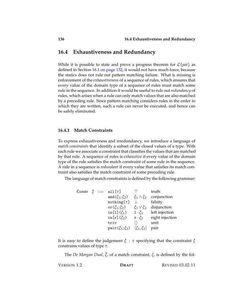
136 16.4 Exhaustiveness and Redundancy
16.4 Exhaustiveness and Redundancy
While it is possible to state and prove a progress theorem for L{pat} asdefined in Section 16.1 on page 132, it would not have much force, becausethe statics does not rule out pattern matching failure. What is missing isenforcement of the exhaustiveness of a sequence of rules, which ensures thatevery value of the domain type of a sequence of rules must match somerule in the sequence. In addition it would be useful to rule out redundancy ofrules, which arises when a rule can only match values that are also matchedby a preceding rule. Since pattern matching considers rules in the order inwhich they are written, such a rule can never be executed, and hence canbe safely eliminated.
16.4.1 Match Constraints
To express exhaustiveness and irredundancy, we introduce a language ofmatch constraints that identify a subset of the closed values of a type. Witheach rule we associate a constraint that classifies the values that are matchedby that rule. A sequence of rules is exhaustive if every value of the domaintype of the rule satisfies the match constraint of some rule in the sequence.A rule in a sequence is redundant if every value that satisfies its match con-traint also satisfies the match constraint of some preceding rule.
The language of match constraints is defined by the following grammar:
Constr + ::= all["] F truthand(+1; +2) +1 4 +2 conjunctionnothing["] > falsityor(+1; +2) +1 G +2 disjunctionin[l](+1) l · +1 left injectionin[r](+2) r · +2 right injectiontriv ?@ unitpair(+1; +2) ?+1, +2@ pair
It is easy to define the judgement + : " specifying that the constraint +constrains values of type ".
The De Morgan Dual, +, of a match constraint, +, is defined by the fol-
VERSION 1.2 DRAFT REVISED 03.02.11
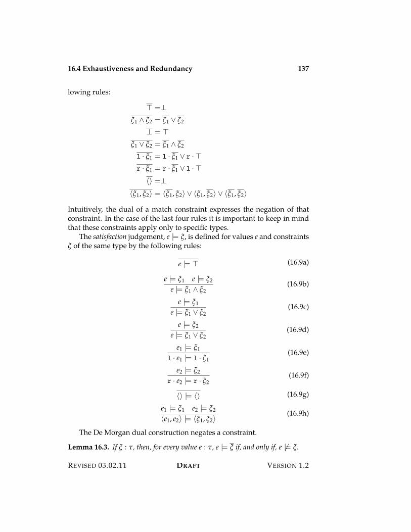
16.4 Exhaustiveness and Redundancy 137
lowing rules:
F =>+1 4 +2 = +1 G +2
> = F+1 G +2 = +1 4 +2
l · +1 = l · +1 G r ·Fr · +1 = r · +1 G l ·F
?@ =>?+1, +2@ = ?+1, +2@ G ?+1, +2@ G ?+1, +2@
Intuitively, the dual of a match constraint expresses the negation of thatconstraint. In the case of the last four rules it is important to keep in mindthat these constraints apply only to specific types.
The satisfaction judgement, e |= +, is defined for values e and constraints+ of the same type by the following rules:
e |= F (16.9a)
e |= +1 e |= +2
e |= +1 4 +2(16.9b)
e |= +1
e |= +1 G +2(16.9c)
e |= +2
e |= +1 G +2(16.9d)
e1 |= +1
l · e1 |= l · +1(16.9e)
e2 |= +2
r · e2 |= r · +2(16.9f)
?@ |= ?@ (16.9g)
e1 |= +1 e2 |= +2
?e1, e2@ |= ?+1, +2@(16.9h)
The De Morgan dual construction negates a constraint.
Lemma 16.3. If + : ", then, for every value e : ", e |= + if, and only if, e ,|= +.
REVISED 03.02.11 DRAFT VERSION 1.2
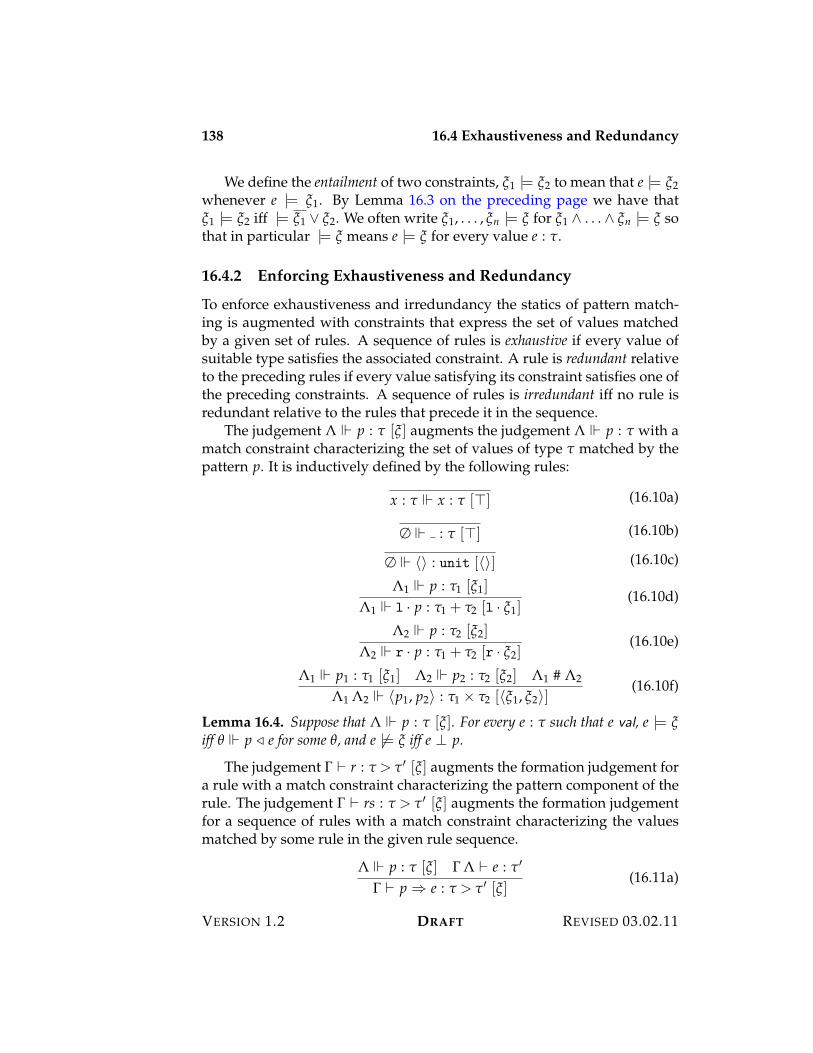
138 16.4 Exhaustiveness and Redundancy
We define the entailment of two constraints, +1 |= +2 to mean that e |= +2whenever e |= +1. By Lemma 16.3 on the preceding page we have that+1 |= +2 iff |= +1 G +2. We often write +1, . . . , +n |= + for +1 4 . . . 4 +n |= + sothat in particular |= + means e |= + for every value e : ".
16.4.2 Enforcing Exhaustiveness and Redundancy
To enforce exhaustiveness and irredundancy the statics of pattern match-ing is augmented with constraints that express the set of values matchedby a given set of rules. A sequence of rules is exhaustive if every value ofsuitable type satisfies the associated constraint. A rule is redundant relativeto the preceding rules if every value satisfying its constraint satisfies one ofthe preceding constraints. A sequence of rules is irredundant iff no rule isredundant relative to the rules that precede it in the sequence.
The judgement ( $ p : " [+] augments the judgement ( $ p : " with amatch constraint characterizing the set of values of type " matched by thepattern p. It is inductively defined by the following rules:
x : " $ x : " [F] (16.10a)
# $ : " [F] (16.10b)
# $ ?@ : unit [?@] (16.10c)
(1 $ p : "1 [+1]
(1 $ l · p : "1 + "2 [l · +1](16.10d)
(2 $ p : "2 [+2]
(2 $ r · p : "1 + "2 [r · +2](16.10e)
(1 $ p1 : "1 [+1] (2 $ p2 : "2 [+2] (1 # (2
(1 (2 $ ?p1, p2@ : "1 < "2 [?+1, +2@](16.10f)
Lemma 16.4. Suppose that ( $ p : " [+]. For every e : " such that e val, e |= +iff * $ p # e for some *, and e ,|= + iff e > p.
The judgement ! ) r : " > "% [+] augments the formation judgement fora rule with a match constraint characterizing the pattern component of therule. The judgement ! ) rs : " > "% [+] augments the formation judgementfor a sequence of rules with a match constraint characterizing the valuesmatched by some rule in the given rule sequence.
( $ p : " [+] ! ( ) e : "%
! ) p ; e : " > "% [+](16.11a)
VERSION 1.2 DRAFT REVISED 03.02.11
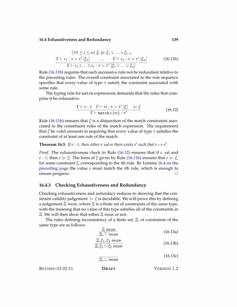
16.4 Exhaustiveness and Redundancy 139
(&1 ( i ( n) +i ,|= +1 G . . . G +i$1
! ) r1 : " > "% [+1] . . . ! ) rn : " > "% [+n]
! ) r1 | . . . | rn : " > "% [+1 G . . . G +n]
(16.11b)
Rule (16.11b) requires that each successive rule not be redundant relative tothe preceding rules. The overall constraint associated to the rule sequencespecifies that every value of type " satisfy the constraint associated withsome rule.
The typing rule for match expressions demands that the rules that com-prise it be exhaustive:
! ) e : " ! ) rs : " > "% [+] |= +
! ) match e {rs} : "% (16.12)
Rule (16.11b) ensures that + is a disjunction of the match constraints asso-ciated to the constituent rules of the match expression. The requirementthat + be valid amounts to requiring that every value of type " satisfies theconstraint of at least one rule of the match.
Theorem 16.5. If e : ", then either e val or there exists e% such that e 53 e%.
Proof. The exhaustiveness check in Rule (16.12) ensures that if e val ande : ", then e |= +. The form of + given by Rule (16.11b) ensures that e |= +ifor some constraint +i corresponding to the ith rule. By Lemma 16.4 on thepreceding page the value e must match the ith rule, which is enough toensure progress.
16.4.3 Checking Exhaustiveness and Redundancy
Checking exhaustiveness and redundacy reduces to showing that the con-straint validity judgement |= + is decidable. We will prove this by defininga judgement % incon, where % is a finite set of constraints of the same type,with the meaning that no value of this type satisfies all of the constraints in%. We will then show that either % incon or not.
The rules defining inconsistency of a finite set, %, of constraints of thesame type are as follows:
% incon%,F incon
(16.13a)
%, +1, +2 incon
%, +1 4 +2 incon(16.13b)
%,> incon(16.13c)
REVISED 03.02.11 DRAFT VERSION 1.2
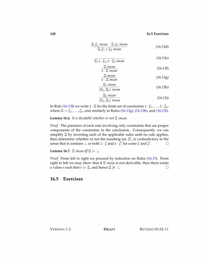
140 16.5 Exercises
%, +1 incon %, +2 incon
%, +1 G +2 incon(16.13d)
%, l · +1, r · +2 incon(16.13e)
% inconl · % incon
(16.13f)
% inconr · % incon
(16.13g)
%1 incon
?%1, %2@ incon(16.13h)
%2 incon
?%1, %2@ incon(16.13i)
In Rule (16.13f) we write l ·% for the finite set of constraints l · +1, . . . , l · +n,where % = +1, . . . , +n, and similarly in Rules (16.13g), (16.13h), and (16.13i).
Lemma 16.6. It is decidable whether or not % incon.
Proof. The premises of each rule involving only constraints that are propercomponents of the constraints in the conclusion. Consequently, we cansimplify % by inverting each of the applicable rules until no rule applies,then determine whether or not the resulting set, %%, is contradictory in thesense that it contains > or both l · + and r · + % for some + and + %.
Lemma 16.7. % incon iff % |= >.
Proof. From left to right we proceed by induction on Rules (16.13). Fromright to left we may show that if % incon is not derivable, then there existsa value e such that e |= %, and hence % ,|= >.
16.5 Exercises
VERSION 1.2 DRAFT REVISED 03.02.11
Chapter 17
Generic Programming
17.1 Introduction
Many programs can be seen as instances of a general pattern applied to aparticular situation. Very often the pattern is determined by the types ofthe data involved. For example, in Chapter 12 the pattern of computing byrecursion over a natural number is isolated as the defining characteristic ofthe type of natural numbers. This concept will itself emerge as an instanceof the concept of type-generic, or just generic, programming.
Suppose that we have a function, f , of type & 3 &% that transforms val-ues of type & into values of type &%. For example, f might be the doublingfunction on natural numbers. We wish to extend f to a transformationfrom type [&/t]" to type [&%/t]" by applying f to various spots in the inputwhere a value of type & occurs to obtain a value of type &%, leaving the restof the data structure alone. For example, " might be bool < &, in whichcase f could be extended to a function of type bool< & 3 bool< &% thatsends the pairs ?a, b@ to the pair ?a, f(b)@.
This example glosses over a significant problem of ambiguity of the ex-tension. Given a function f of type & 3 &%, it is not obvious in generalhow to extend it to a function mapping [&/t]" to [&%/t]". The problemis that it is not clear which of many occurrences of & in [&/t]" are to betransformed by f , even if there is only one occurrence of &. To avoid am-biguity we need a way to mark which occurrences of & in [&/t]" are to betransformed, and which are to be left fixed. This can be achieved by isolat-ing the type operator, t.", which is a type expression in which a designatedvariable, t, marks the spots at which we wish the transformation to occur.Given t." and f : & 3 &%, we can extend f unambiguously to a function of
142 17.2 Type Operators
type [&/t]" 3 [&%/t]".The technique of using a type operator to determine the behavior of
a piece of code is called generic programming. The power of generic pro-gramming depends on which forms of type operator are considered. Thesimplest case is that of a polynomial type operator, one constructed fromsum and product of types, including their nullary forms. These may beextended to positive type operators, which also permit restricted forms offunction types.
17.2 Type Operators
A type operator is a type equipped with a designated variable whose oc-currences mark the positions in the type where a transformation is to beapplied. A type operator is represented by an abstractor t." such thatt type ) " type. An example of a type operator is the abstractor
t.unit+ (bool< t)
in which occurrences of t mark the spots in which a transformation is tobe applied. An instance of the type operator t." is obtained by substitut-ing a type, &, for the variable, t, within the type ". We sometimes writeMap[t."](&) for the substitution instance [&/t]".
The polynomial type operators are those constructed from the type vari-able, t, the types void and unit, and the product and sum type construc-tors, "1 < "2 and "1 + "2. It is a straightforward exercise to give inductivedefinitions of the judgement t." poly stating that the operator t." is a poly-nomial type operator.
17.3 Generic Extension
The generic extension primitive has the form
map[t."](x.e%; e)
with statics given by the following rule:
t type ) " type !, x : & ) e% : &% ! ) e : [&/t]"! ) map[t."](x.e%; e) : [&%/t]"
(17.1)
The abstractor x.e% specifies a transformation from type &, the type of x, totype &%, the type of e%. The expression e of type [&/t]" determines the value
VERSION 1.2 DRAFT REVISED 03.02.11
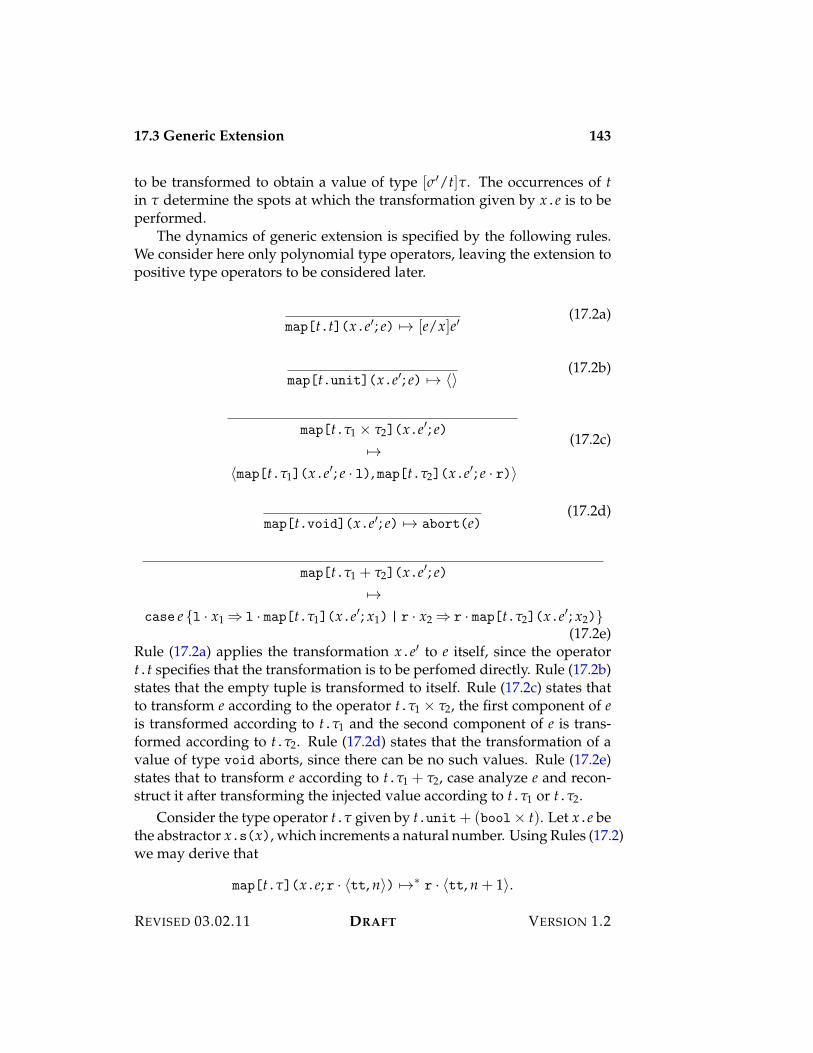
17.3 Generic Extension 143
to be transformed to obtain a value of type [&%/t]". The occurrences of tin " determine the spots at which the transformation given by x.e is to beperformed.
The dynamics of generic extension is specified by the following rules.We consider here only polynomial type operators, leaving the extension topositive type operators to be considered later.
map[t.t](x.e%; e) 53 [e/x]e%(17.2a)
map[t.unit](x.e%; e) 53 ?@(17.2b)
map[t."1 < "2](x.e%; e)53
?map[t."1](x.e%; e · l), map[t."2](x.e%; e · r)@
(17.2c)
map[t.void](x.e%; e) 53 abort(e)(17.2d)
map[t."1 + "2](x.e%; e)53
case e {l · x1 ; l · map[t."1](x.e%; x1) | r · x2 ; r · map[t."2](x.e%; x2)}(17.2e)
Rule (17.2a) applies the transformation x.e% to e itself, since the operatort.t specifies that the transformation is to be perfomed directly. Rule (17.2b)states that the empty tuple is transformed to itself. Rule (17.2c) states thatto transform e according to the operator t."1 < "2, the first component of eis transformed according to t."1 and the second component of e is trans-formed according to t."2. Rule (17.2d) states that the transformation of avalue of type void aborts, since there can be no such values. Rule (17.2e)states that to transform e according to t."1 + "2, case analyze e and recon-struct it after transforming the injected value according to t."1 or t."2.
Consider the type operator t." given by t.unit+ (bool< t). Let x.e bethe abstractor x.s(x), which increments a natural number. Using Rules (17.2)we may derive that
map[t."](x.e; r · ?tt, n@) 531 r · ?tt, n + 1@.
REVISED 03.02.11 DRAFT VERSION 1.2
144 17.3 Generic Extension
The natural number in the second component of the pair is incremented,since the type variable, t, occurs in that position in the type operator t.".
Theorem 17.1 (Preservation). If map[t."](x.e%; e) : , and map[t."](x.e%; e) 53e%%, then e%% : ,.
Proof. By inversion of Rule (17.1) we have
1. t type ) " type;
2. x : & ) e% : &% for some & and &%;
3. e : [&/t]";
4. , is [&%/t]".
We proceed by cases on Rules (17.2). For example, consider Rule (17.2c). Itfollows from inversion that map[t."1](x.e%; e · l) : [&%/t]"1, and similarlythat map[t."2](x.e%; e · r) : [&%/t]"2. It is easy to check that
?map[t."1](x.e%; e · l), map[t."2](x.e%; e · r)@
has type [&%/t]"1 < "2, as required.
The positive type operators extend the polynomial type operators to ad-mit restricted forms of function type. Specifically, t."1 3 "2 is a positivetype operator, provided that (1) t does not occur in "1, and (2) t."2 is a pos-itive type operator. In general, any occurrences of a type variable t in thedomain a function type are said to be negative occurrences, whereas any oc-currences of t within the range of a function type, or within a product orsum type, are said to be positive occurrences.1 A positive type operator isone for which only positive occurrences of the parameter, t, are permitted.
The generic extension according to a positive type operator is definedsimilarly to the case of a polynomial type operator, with the following ad-ditional rule:
map[t."1 3 "2](x.e%; e) 53 ! (x1:"1. map[t."2](x.e%; e(x1)))(17.3)
1The origin of this terminology appears to be that a function type "1 3 "2 is, by thepropositions-as-types principle, analogous to the implication '1 H '2, which is classicallyequivalent to ¬'1 G '2, placing occurrences in the domain beneath the negation sign.
VERSION 1.2 DRAFT REVISED 03.02.11
17.4 Exercises 145
Since t is not permitted to occur within the domain type, the type of theresult is "1 3 [&%/t]"2, assuming that e is of type "1 3 [&/t]"2. It is easy toverify preservation for the generic extension of a positive type operator.
It is interesting to consider what goes wrong if we relax the restric-tion on positive type operators to admit negative, as well as positive, oc-currences of the parameter of a type operator. Consider the type opera-tor t."1 3 "2, without restriction on t, and suppose that x : & ) e% : &%.The generic extension map[t."1 3 "2](x.e%; e) should have type [&%/t]"1 3[&%/t]"2, given that e has type [&/t]"1 3 [&/t]"2. The extension shouldyield a function of the form
! (x1:[&%/t]"1. . . .(e(. . .(x1))))
in which we apply e to a transformation of x1 and then transform the re-sult. The trouble is that we are given, inductively, that map[t."1](x.e%;$)
transforms values of type [&/t]"1 into values of type [&%/t]"1, but we needto go the other way around in order to make x1 suitable as an argument for e.But there is no obvious way to obtain the required transformation.
One solution to this is to assume that the fundamental transformationx.e% is invertible so that we may apply the inverse transformation on x1 toget an argument of type suitable for e, then apply the forward transforma-tion on the result, just as in the positive case. Since we cannot invert an ar-bitrary transformation, we must instead pass both the transformation andits inverse to the generic extension operation so that it can “go backwards”as necessary to cover negative occurrences of the type parameter. So in thegeneral case the generic extension applies only when we are given a typeisomorphism (a pair of mutually inverse mappings between two types), andthen results in another isomorphism pair. We leave the formulation of thisas an exercise for the reader.
17.4 Exercises
REVISED 03.02.11 DRAFT VERSION 1.2

146 17.4 Exercises
VERSION 1.2 DRAFT REVISED 03.02.11
Part VI
Infinite Data Types

Chapter 18
Inductive and Co-InductiveTypes
The inductive and the coinductive types are two important forms of recur-sive type. Inductive types correspond to least, or initial, solutions of certaintype isomorphism equations, and coinductive types correspond to theirgreatest, or final, solutions. Intuitively, the elements of an inductive typeare those that may be obtained by a finite composition of its introductoryforms. Consequently, if we specify the behavior of a function on each of theintroductory forms of an inductive type, then its behavior is determined forall values of that type. Such a function is called a recursor, or catamorphism.Dually, the elements of a coinductive type are those that behave properlyin response to a finite composition of its elimination forms. Consequently,if we specify the behavior of an element on each elimination form, then wehave fully specified that element as a value of that type. Such an element iscalled an generator, or anamorphism.
18.1 Motivating Examples
The most important example of an inductive type is the type of naturalnumbers as formalized in Chapter 12. The type nat is defined to be theleast type containing z and closed under s($). The minimality conditionis witnessed by the existence of the recursor, natiter e {z;e0 | s(x);e1},which transforms a natural number into a value of type ", given its valuefor zero, and a transformation from its value on a number to its value on thesuccessor of that number. This operation is well-defined precisely becausethere are no other natural numbers. Put the other way around, the existence
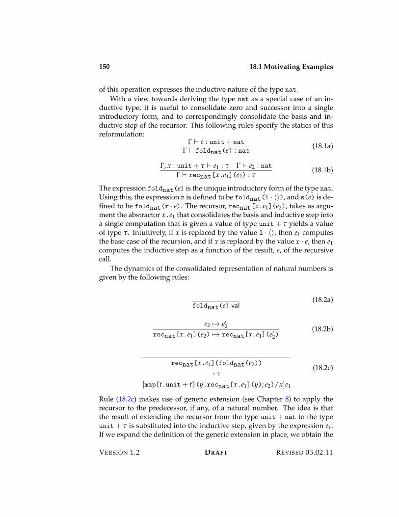
150 18.1 Motivating Examples
of this operation expresses the inductive nature of the type nat.With a view towards deriving the type nat as a special case of an in-
ductive type, it is useful to consolidate zero and successor into a singleintroductory form, and to correspondingly consolidate the basis and in-ductive step of the recursor. This following rules specify the statics of thisreformulation:
! ) e : unit+ nat! ) foldnat(e) : nat (18.1a)
!, x : unit+ " ) e1 : " ! ) e2 : nat! ) recnat[x.e1](e2) : "
(18.1b)
The expression foldnat(e) is the unique introductory form of the type nat.Using this, the expression z is defined to be foldnat(l · ?@), and s(e) is de-fined to be foldnat(r · e). The recursor, recnat[x.e1](e2), takes as argu-ment the abstractor x.e1 that consolidates the basis and inductive step intoa single computation that is given a value of type unit+ " yields a valueof type ". Intuitively, if x is replaced by the value l · ?@, then e1 computesthe base case of the recursion, and if x is replaced by the value r · e, then e1computes the inductive step as a function of the result, e, of the recursivecall.
The dynamics of the consolidated representation of natural numbers isgiven by the following rules:
foldnat(e) val(18.2a)
e2 53 e%2recnat[x.e1](e2) 53 recnat[x.e1](e%2)
(18.2b)
recnat[x.e1](foldnat(e2))
53[map[t.unit+ t](y.recnat[x.e1](y); e2)/x]e1
(18.2c)
Rule (18.2c) makes use of generic extension (see Chapter 8) to apply therecursor to the predecessor, if any, of a natural number. The idea is thatthe result of extending the recursor from the type unit+ nat to the typeunit+ " is substituted into the inductive step, given by the expression e1.If we expand the definition of the generic extension in place, we obtain the
VERSION 1.2 DRAFT REVISED 03.02.11

18.1 Motivating Examples 151
following reformulation of this rule:
recnat[x.e1](foldnat(e2))
53[case e2 {l · ; l · ?@ | r · y ; r · recnat[x.e1](y)}/x]e1
An illustrative example of a coinductive type is the type of streams ofnatural numbers. A stream is an infinite sequence of natural numbers suchthat an element of the stream can be computed only after computing allpreceding elements in that stream. That is, the computations of successiveelements of the stream are sequentially dependent in that the computationof one element influences the computation of the next. This characteristicof the introductory form for streams is dual to the analogous property ofthe eliminatory form for natural numbers whereby the result for a numberis determined by its result for all preceding numbers.
A stream is characterized by its behavior under the elimination formsfor the stream type: hd(e) returns the next, or head, element of the stream,and tl(e) returns the tail of the stream, the stream resulting when the headelement is removed. A stream is introduced by a generator, the dual of arecursor, that determines the head and the tail of the stream in terms of thecurrent state of the stream, which is represented by a value of some type.The statics of streams is given by the following rules:
! ) e : stream! ) hd(e) : nat (18.3a)
! ) e : stream! ) tl(e) : stream (18.3b)
! ) e : " !, x : " ) e1 : nat !, x : " ) e2 : "! ) strgen e <hd(x); e1 & tl(x); e2> : stream
(18.3c)
In Rule (18.3c) the current state of the stream is given by the expression eof some type ", and the head and tail of the stream are determined by theexpressions e1 and e2, respectively, as a function of the current state.
The dynamics of streams is given by the following rules:
strgen e <hd(x); e1 & tl(x); e2> val(18.4a)
e 53 e%hd(e) 53 hd(e%)
(18.4b)
REVISED 03.02.11 DRAFT VERSION 1.2
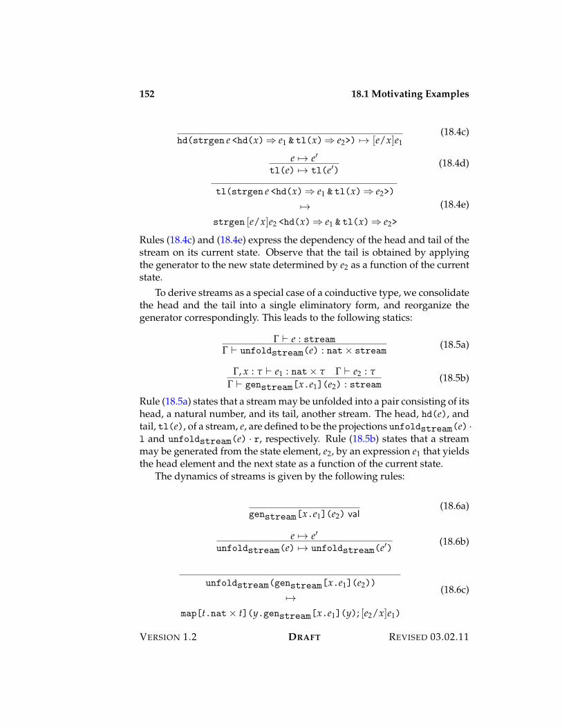
152 18.1 Motivating Examples
hd(strgen e <hd(x); e1 & tl(x); e2>) 53 [e/x]e1(18.4c)
e 53 e%tl(e) 53 tl(e%)
(18.4d)
tl(strgen e <hd(x); e1 & tl(x); e2>)
53strgen [e/x]e2 <hd(x); e1 & tl(x); e2>
(18.4e)
Rules (18.4c) and (18.4e) express the dependency of the head and tail of thestream on its current state. Observe that the tail is obtained by applyingthe generator to the new state determined by e2 as a function of the currentstate.
To derive streams as a special case of a coinductive type, we consolidatethe head and the tail into a single eliminatory form, and reorganize thegenerator correspondingly. This leads to the following statics:
! ) e : stream! ) unfoldstream(e) : nat< stream
(18.5a)
!, x : " ) e1 : nat< " ! ) e2 : "! ) genstream[x.e1](e2) : stream (18.5b)
Rule (18.5a) states that a stream may be unfolded into a pair consisting of itshead, a natural number, and its tail, another stream. The head, hd(e), andtail, tl(e), of a stream, e, are defined to be the projections unfoldstream(e) ·l and unfoldstream(e) · r, respectively. Rule (18.5b) states that a streammay be generated from the state element, e2, by an expression e1 that yieldsthe head element and the next state as a function of the current state.
The dynamics of streams is given by the following rules:
genstream[x.e1](e2) val(18.6a)
e 53 e%unfoldstream(e) 53 unfoldstream(e%) (18.6b)
unfoldstream(genstream[x.e1](e2))
53map[t.nat< t](y.genstream[x.e1](y); [e2/x]e1)
(18.6c)
VERSION 1.2 DRAFT REVISED 03.02.11
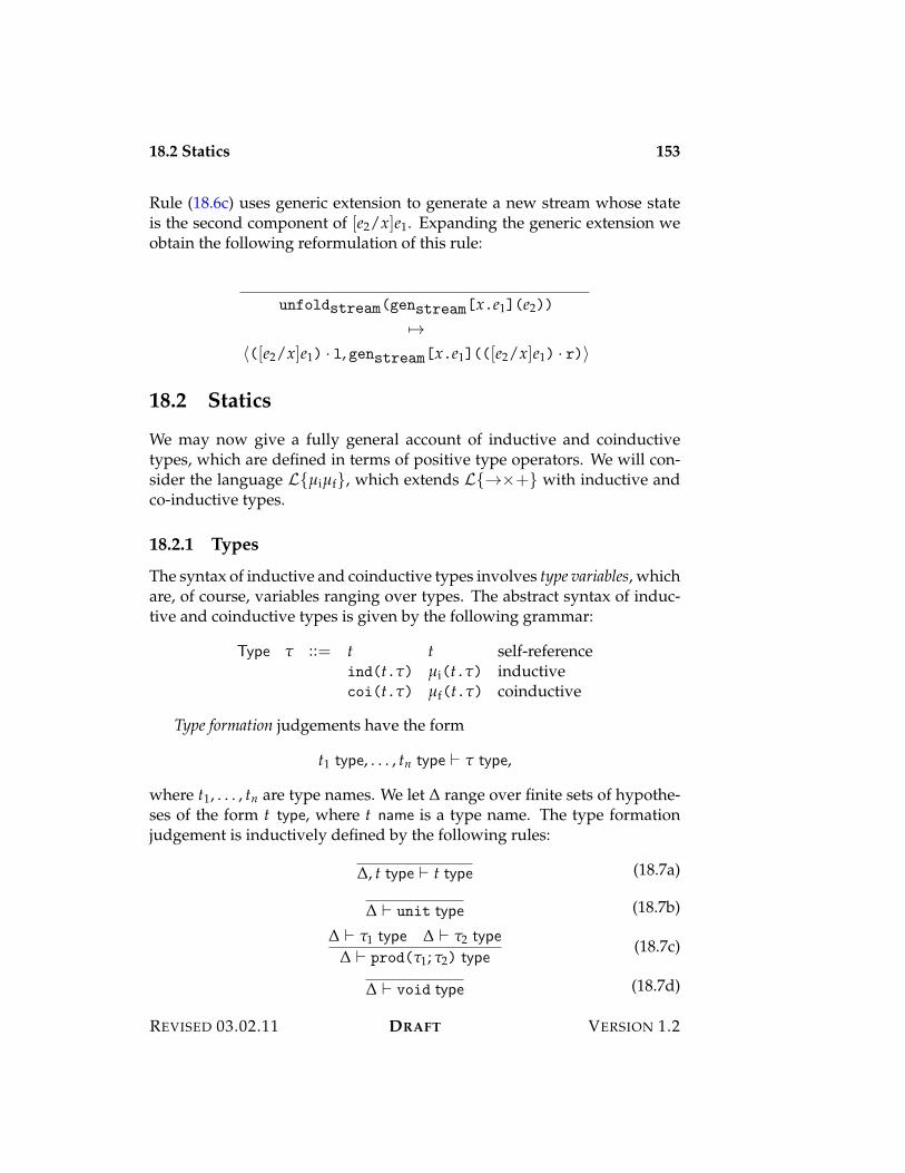
18.2 Statics 153
Rule (18.6c) uses generic extension to generate a new stream whose stateis the second component of [e2/x]e1. Expanding the generic extension weobtain the following reformulation of this rule:
unfoldstream(genstream[x.e1](e2))
53?([e2/x]e1) · l, genstream[x.e1](([e2/x]e1) · r)@
18.2 Statics
We may now give a fully general account of inductive and coinductivetypes, which are defined in terms of positive type operators. We will con-sider the language L{µiµf}, which extends L{3<+} with inductive andco-inductive types.
18.2.1 Types
The syntax of inductive and coinductive types involves type variables, whichare, of course, variables ranging over types. The abstract syntax of induc-tive and coinductive types is given by the following grammar:
Type " ::= t t self-referenceind(t.") µi(t.") inductivecoi(t.") µf(t.") coinductive
Type formation judgements have the form
t1 type, . . . , tn type ) " type,
where t1, . . . , tn are type names. We let " range over finite sets of hypothe-ses of the form t type, where t name is a type name. The type formationjudgement is inductively defined by the following rules:
", t type ) t type (18.7a)
" ) unit type (18.7b)
" ) "1 type " ) "2 type" ) prod("1; "2) type
(18.7c)
" ) void type (18.7d)
REVISED 03.02.11 DRAFT VERSION 1.2
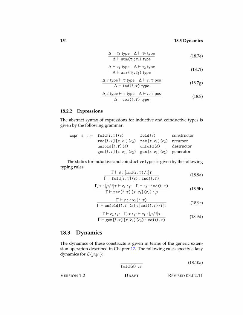
154 18.3 Dynamics
" ) "1 type " ) "2 type" ) sum("1; "2) type
(18.7e)
" ) "1 type " ) "2 type" ) arr("1; "2) type
(18.7f)
", t type ) " type " ) t." pos" ) ind(t.") type
(18.7g)
", t type ) " type " ) t." pos" ) coi(t.") type
(18.8)
18.2.2 Expressions
The abstract syntax of expressions for inductive and coinductive types isgiven by the following grammar:
Expr e ::= fold[t."](e) fold(e) constructorrec[t."][x.e1](e2) rec[x.e1](e2) recursorunfold[t."](e) unfold(e) destructorgen[t."][x.e1](e2) gen[x.e1](e2) generator
The statics for inductive and coinductive types is given by the followingtyping rules:
! ) e : [ind(t.")/t]"! ) fold[t."](e) : ind(t.")
(18.9a)
!, x : [,/t]" ) e1 : , ! ) e2 : ind(t.")
! ) rec[t."][x.e1](e2) : ,(18.9b)
! ) e : coi(t.")! ) unfold[t."](e) : [coi(t.")/t]" (18.9c)
! ) e2 : , !, x : , ) e1 : [,/t]"! ) gen[t."][x.e1](e2) : coi(t.")
(18.9d)
18.3 Dynamics
The dynamics of these constructs is given in terms of the generic exten-sion operation described in Chapter 17. The following rules specify a lazydynamics for L{µiµf}:
fold(e) val(18.10a)
VERSION 1.2 DRAFT REVISED 03.02.11
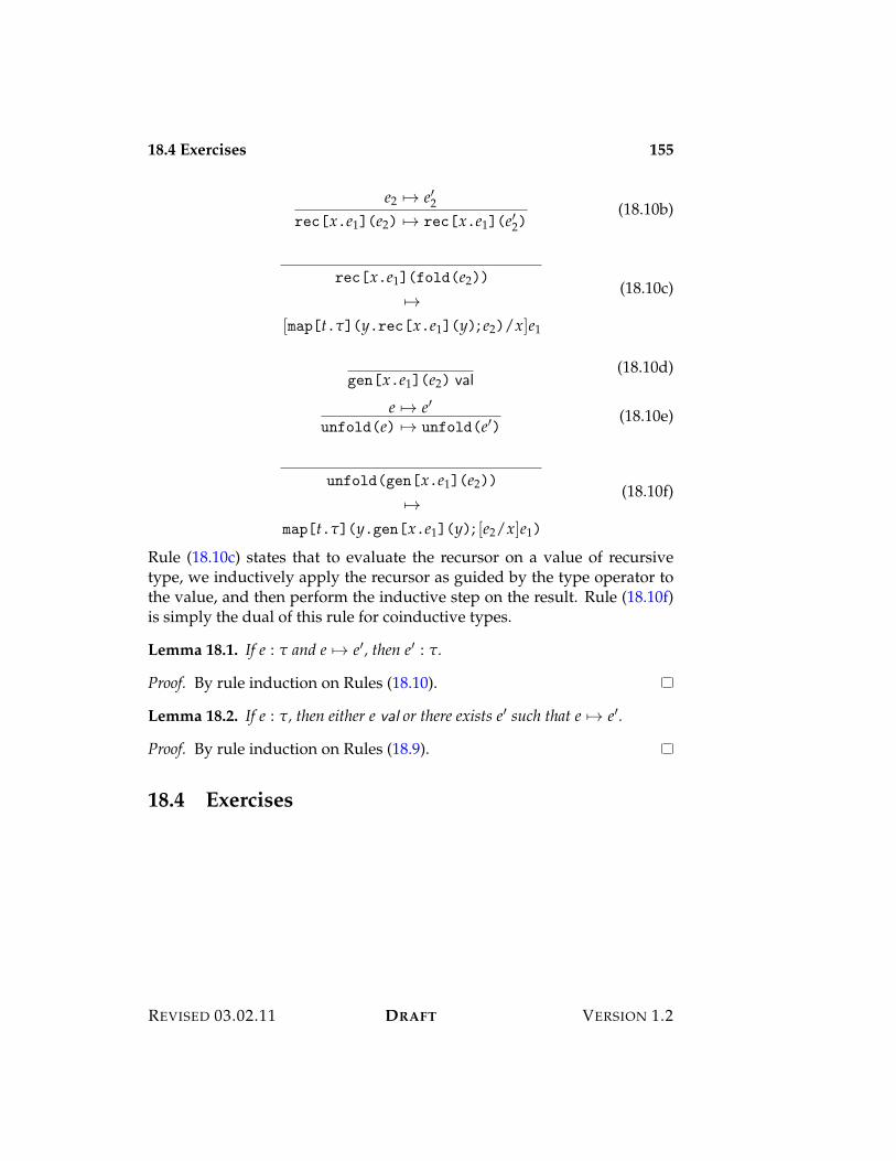
18.4 Exercises 155
e2 53 e%2rec[x.e1](e2) 53 rec[x.e1](e%2)
(18.10b)
rec[x.e1](fold(e2))
53[map[t."](y.rec[x.e1](y); e2)/x]e1
(18.10c)
gen[x.e1](e2) val(18.10d)
e 53 e%unfold(e) 53 unfold(e%)
(18.10e)
unfold(gen[x.e1](e2))
53map[t."](y.gen[x.e1](y); [e2/x]e1)
(18.10f)
Rule (18.10c) states that to evaluate the recursor on a value of recursivetype, we inductively apply the recursor as guided by the type operator tothe value, and then perform the inductive step on the result. Rule (18.10f)is simply the dual of this rule for coinductive types.
Lemma 18.1. If e : " and e 53 e%, then e% : ".
Proof. By rule induction on Rules (18.10).
Lemma 18.2. If e : ", then either e val or there exists e% such that e 53 e%.
Proof. By rule induction on Rules (18.9).
18.4 Exercises
REVISED 03.02.11 DRAFT VERSION 1.2

156 18.4 Exercises
VERSION 1.2 DRAFT REVISED 03.02.11
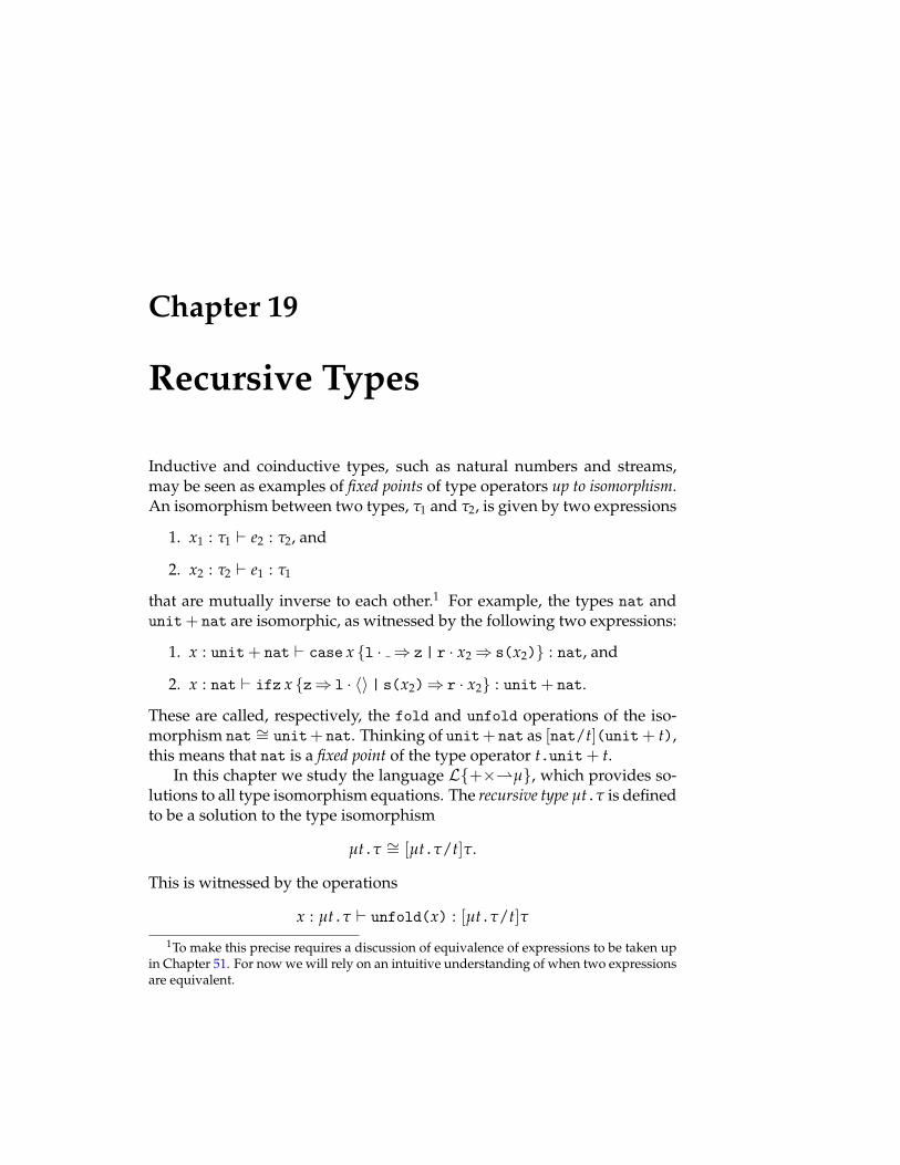
Chapter 19
Recursive Types
Inductive and coinductive types, such as natural numbers and streams,may be seen as examples of fixed points of type operators up to isomorphism.An isomorphism between two types, "1 and "2, is given by two expressions
1. x1 : "1 ) e2 : "2, and
2. x2 : "2 ) e1 : "1
that are mutually inverse to each other.1 For example, the types nat andunit+ nat are isomorphic, as witnessed by the following two expressions:
1. x : unit+ nat ) case x {l · ; z | r · x2 ; s(x2)} : nat, and
2. x : nat ) ifz x {z; l · ?@ | s(x2); r · x2} : unit+ nat.
These are called, respectively, the fold and unfold operations of the iso-morphism nat I= unit+ nat. Thinking of unit+ nat as [nat/t](unit+ t),this means that nat is a fixed point of the type operator t.unit+ t.
In this chapter we study the language L{+<"µ}, which provides so-lutions to all type isomorphism equations. The recursive type µt." is definedto be a solution to the type isomorphism
µt." I= [µt."/t]".
This is witnessed by the operations
x : µt." ) unfold(x) : [µt."/t]"1To make this precise requires a discussion of equivalence of expressions to be taken up
in Chapter 51. For now we will rely on an intuitive understanding of when two expressionsare equivalent.
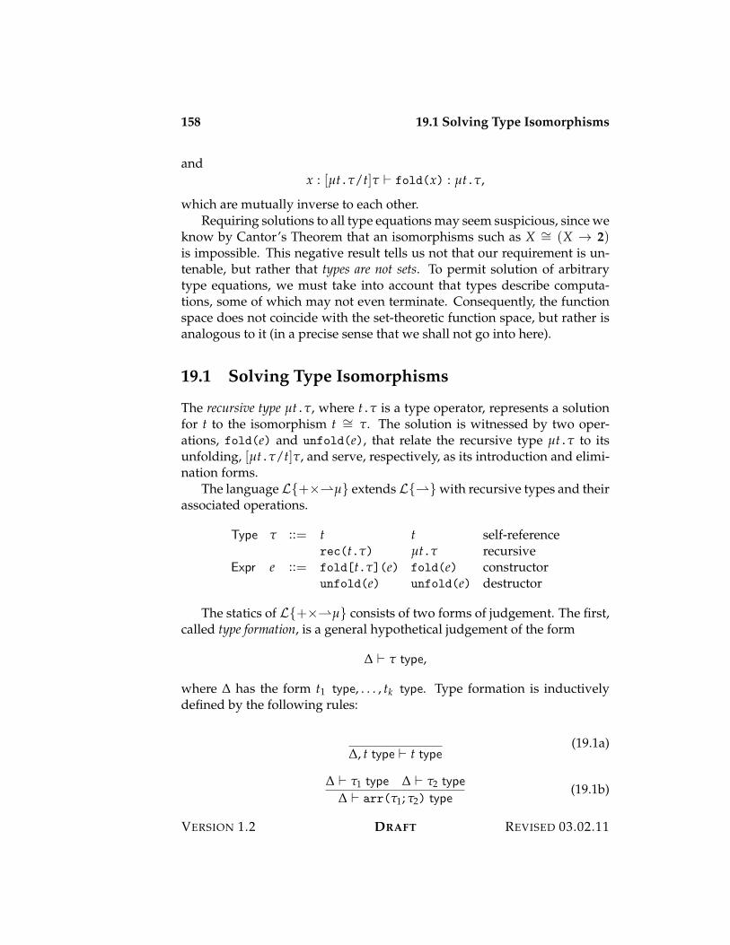
158 19.1 Solving Type Isomorphisms
andx : [µt."/t]" ) fold(x) : µt.",
which are mutually inverse to each other.Requiring solutions to all type equations may seem suspicious, since we
know by Cantor’s Theorem that an isomorphisms such as X I= (X 3 2)is impossible. This negative result tells us not that our requirement is un-tenable, but rather that types are not sets. To permit solution of arbitrarytype equations, we must take into account that types describe computa-tions, some of which may not even terminate. Consequently, the functionspace does not coincide with the set-theoretic function space, but rather isanalogous to it (in a precise sense that we shall not go into here).
19.1 Solving Type Isomorphisms
The recursive type µt.", where t." is a type operator, represents a solutionfor t to the isomorphism t I= ". The solution is witnessed by two oper-ations, fold(e) and unfold(e), that relate the recursive type µt." to itsunfolding, [µt."/t]", and serve, respectively, as its introduction and elimi-nation forms.
The language L{+<"µ} extends L{"} with recursive types and theirassociated operations.
Type " ::= t t self-referencerec(t.") µt." recursive
Expr e ::= fold[t."](e) fold(e) constructorunfold(e) unfold(e) destructor
The statics of L{+<"µ} consists of two forms of judgement. The first,called type formation, is a general hypothetical judgement of the form
" ) " type,
where " has the form t1 type, . . . , tk type. Type formation is inductivelydefined by the following rules:
", t type ) t type(19.1a)
" ) "1 type " ) "2 type" ) arr("1; "2) type
(19.1b)
VERSION 1.2 DRAFT REVISED 03.02.11
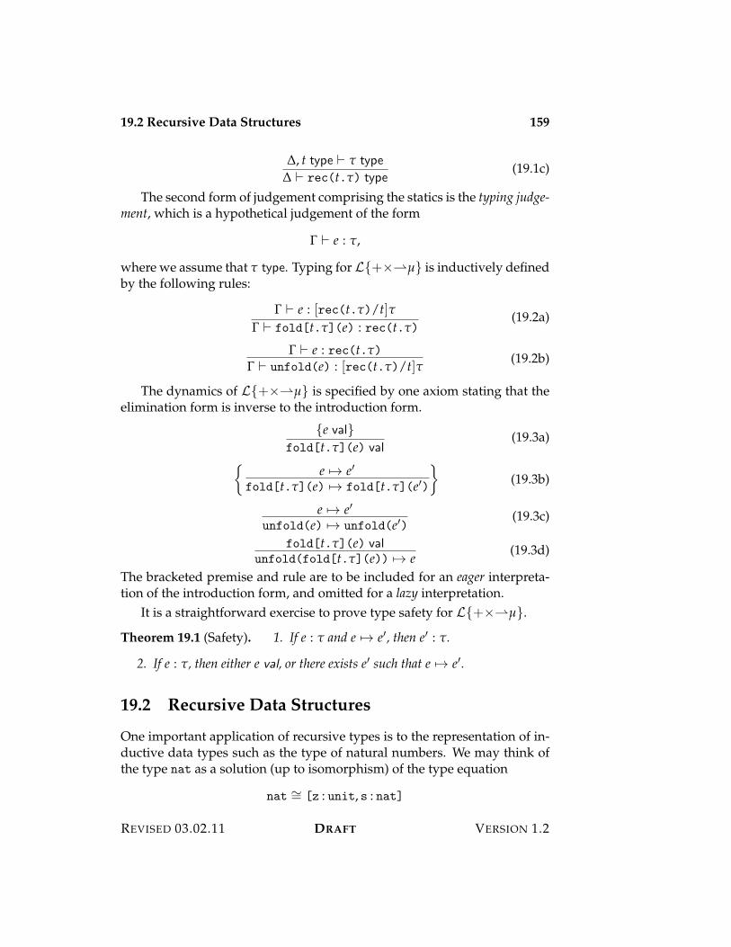
19.2 Recursive Data Structures 159
", t type ) " type" ) rec(t.") type
(19.1c)
The second form of judgement comprising the statics is the typing judge-ment, which is a hypothetical judgement of the form
! ) e : ",
where we assume that " type. Typing for L{+<"µ} is inductively definedby the following rules:
! ) e : [rec(t.")/t]"! ) fold[t."](e) : rec(t.")
(19.2a)
! ) e : rec(t.")! ) unfold(e) : [rec(t.")/t]" (19.2b)
The dynamics of L{+<"µ} is specified by one axiom stating that theelimination form is inverse to the introduction form.
{e val}fold[t."](e) val
(19.3a)
&e 53 e%
fold[t."](e) 53 fold[t."](e%)
'(19.3b)
e 53 e%unfold(e) 53 unfold(e%)
(19.3c)
fold[t."](e) valunfold(fold[t."](e)) 53 e (19.3d)
The bracketed premise and rule are to be included for an eager interpreta-tion of the introduction form, and omitted for a lazy interpretation.
It is a straightforward exercise to prove type safety for L{+<"µ}.
Theorem 19.1 (Safety). 1. If e : " and e 53 e%, then e% : ".
2. If e : ", then either e val, or there exists e% such that e 53 e%.
19.2 Recursive Data Structures
One important application of recursive types is to the representation of in-ductive data types such as the type of natural numbers. We may think ofthe type nat as a solution (up to isomorphism) of the type equation
nat I= [z : unit, s : nat]
REVISED 03.02.11 DRAFT VERSION 1.2
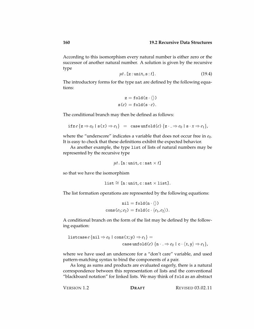
160 19.2 Recursive Data Structures
According to this isomorphism every natural number is either zero or thesuccessor of another natural number. A solution is given by the recursivetype
µt.[z : unit, s : t]. (19.4)
The introductory forms for the type nat are defined by the following equa-tions:
z = fold(z · ?@)s(e) = fold(s · e).
The conditional branch may then be defined as follows:
ifz e {z; e0 | s(x); e1} = case unfold(e) {z · ; e0 | s · x ; e1},
where the “underscore” indicates a variable that does not occur free in e0.It is easy to check that these definitions exhibit the expected behavior.
As another example, the type list of lists of natural numbers may berepresented by the recursive type
µt.[n : unit, c : nat< t]
so that we have the isomorphism
list I= [n : unit, c : nat< list].
The list formation operations are represented by the following equations:
nil = fold(n · ?@)cons(e1; e2) = fold(c · ?e1, e2@).
A conditional branch on the form of the list may be defined by the follow-ing equation:
listcase e {nil; e0 | cons(x; y); e1} =
case unfold(e) {n · ; e0 | c · ?x, y@ ; e1},
where we have used an underscore for a “don’t care” variable, and usedpattern-matching syntax to bind the components of a pair.
As long as sums and products are evaluated eagerly, there is a naturalcorrespondence between this representation of lists and the conventional“blackboard notation” for linked lists. We may think of fold as an abstract
VERSION 1.2 DRAFT REVISED 03.02.11
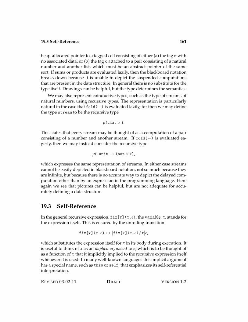
19.3 Self-Reference 161
heap-allocated pointer to a tagged cell consisting of either (a) the tag n withno associated data, or (b) the tag c attached to a pair consisting of a naturalnumber and another list, which must be an abstract pointer of the samesort. If sums or products are evaluated lazily, then the blackboard notationbreaks down because it is unable to depict the suspended computationsthat are present in the data structure. In general there is no substitute for thetype itself. Drawings can be helpful, but the type determines the semantics.
We may also represent coinductive types, such as the type of streams ofnatural numbers, using recursive types. The representation is particularlynatural in the case that fold($) is evaluated lazily, for then we may definethe type stream to be the recursive type
µt.nat< t.
This states that every stream may be thought of as a computation of a pairconsisting of a number and another stream. If fold($) is evaluated ea-gerly, then we may instead consider the recursive type
µt.unit 3 (nat< t),
which expresses the same representation of streams. In either case streamscannot be easily depicted in blackboard notation, not so much because theyare infinite, but because there is no accurate way to depict the delayed com-putation other than by an expression in the programming language. Hereagain we see that pictures can be helpful, but are not adequate for accu-rately defining a data structure.
19.3 Self-Reference
In the general recursive expression, fix["](x.e), the variable, x, stands forthe expression itself. This is ensured by the unrolling transition
fix["](x.e) 53 [fix["](x.e)/x]e,
which substitutes the expression itself for x in its body during execution. Itis useful to think of x as an implicit argument to e, which is to be thought ofas a function of x that it implicitly implied to the recursive expression itselfwhenever it is used. In many well-known languages this implicit argumenthas a special name, such as this or self, that emphasizes its self-referentialinterpretation.
REVISED 03.02.11 DRAFT VERSION 1.2
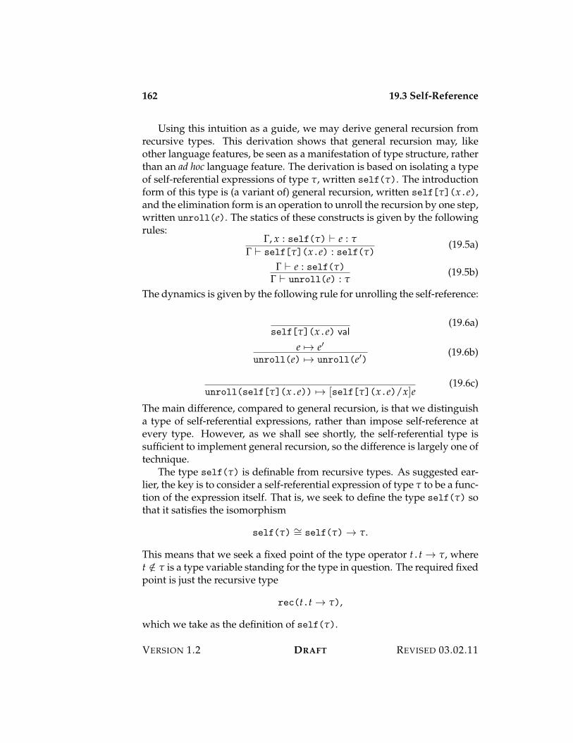
162 19.3 Self-Reference
Using this intuition as a guide, we may derive general recursion fromrecursive types. This derivation shows that general recursion may, likeother language features, be seen as a manifestation of type structure, ratherthan an ad hoc language feature. The derivation is based on isolating a typeof self-referential expressions of type ", written self("). The introductionform of this type is (a variant of) general recursion, written self["](x.e),and the elimination form is an operation to unroll the recursion by one step,written unroll(e). The statics of these constructs is given by the followingrules:
!, x : self(") ) e : "! ) self["](x.e) : self(")
(19.5a)
! ) e : self(")! ) unroll(e) : "
(19.5b)
The dynamics is given by the following rule for unrolling the self-reference:
self["](x.e) val(19.6a)
e 53 e%unroll(e) 53 unroll(e%)
(19.6b)
unroll(self["](x.e)) 53 [self["](x.e)/x]e(19.6c)
The main difference, compared to general recursion, is that we distinguisha type of self-referential expressions, rather than impose self-reference atevery type. However, as we shall see shortly, the self-referential type issufficient to implement general recursion, so the difference is largely one oftechnique.
The type self(") is definable from recursive types. As suggested ear-lier, the key is to consider a self-referential expression of type " to be a func-tion of the expression itself. That is, we seek to define the type self(") sothat it satisfies the isomorphism
self(") I= self(") 3 ".
This means that we seek a fixed point of the type operator t.t 3 ", wheret /+ " is a type variable standing for the type in question. The required fixedpoint is just the recursive type
rec(t.t 3 "),
which we take as the definition of self(").
VERSION 1.2 DRAFT REVISED 03.02.11
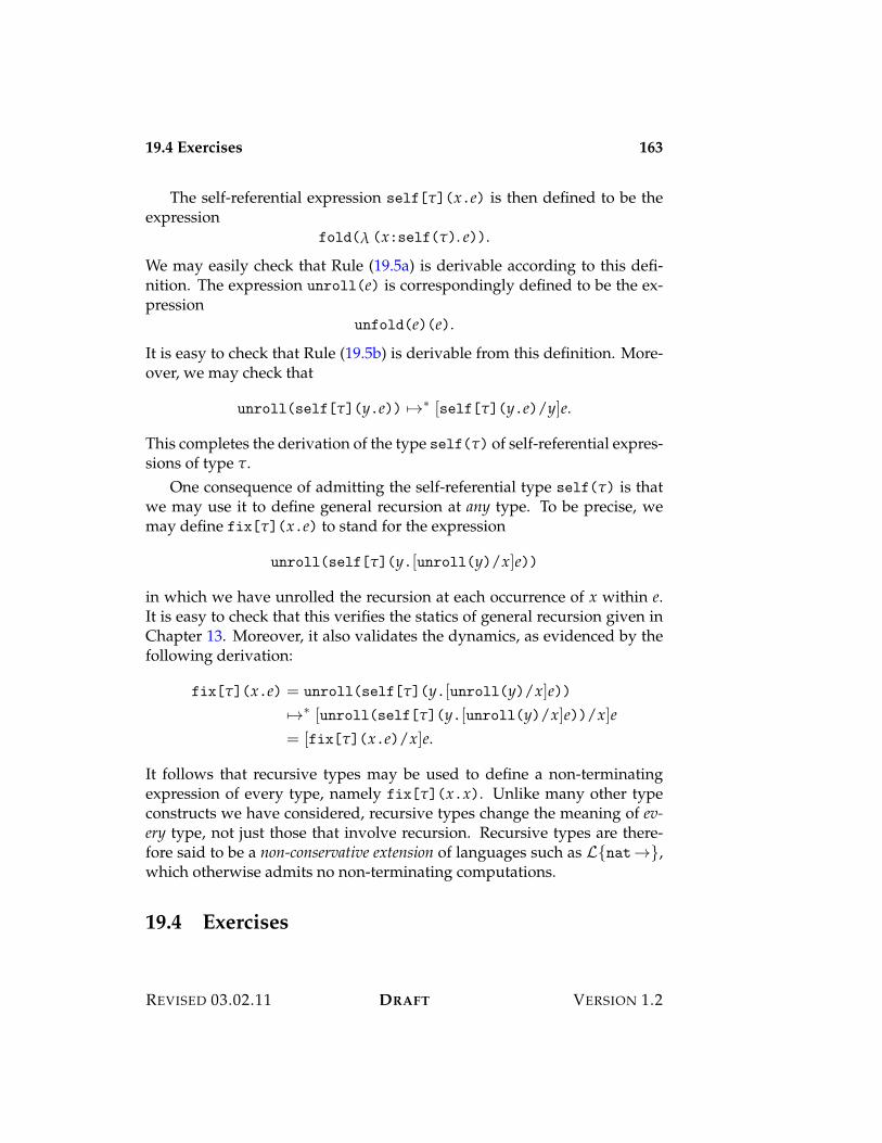
19.4 Exercises 163
The self-referential expression self["](x.e) is then defined to be theexpression
fold(! (x:self("). e)).
We may easily check that Rule (19.5a) is derivable according to this defi-nition. The expression unroll(e) is correspondingly defined to be the ex-pression
unfold(e)(e).
It is easy to check that Rule (19.5b) is derivable from this definition. More-over, we may check that
unroll(self["](y.e)) 531 [self["](y.e)/y]e.
This completes the derivation of the type self(") of self-referential expres-sions of type ".
One consequence of admitting the self-referential type self(") is thatwe may use it to define general recursion at any type. To be precise, wemay define fix["](x.e) to stand for the expression
unroll(self["](y.[unroll(y)/x]e))
in which we have unrolled the recursion at each occurrence of x within e.It is easy to check that this verifies the statics of general recursion given inChapter 13. Moreover, it also validates the dynamics, as evidenced by thefollowing derivation:
fix["](x.e) = unroll(self["](y.[unroll(y)/x]e))531 [unroll(self["](y.[unroll(y)/x]e))/x]e= [fix["](x.e)/x]e.
It follows that recursive types may be used to define a non-terminatingexpression of every type, namely fix["](x.x). Unlike many other typeconstructs we have considered, recursive types change the meaning of ev-ery type, not just those that involve recursion. Recursive types are there-fore said to be a non-conservative extension of languages such as L{nat3},which otherwise admits no non-terminating computations.
19.4 Exercises
REVISED 03.02.11 DRAFT VERSION 1.2

164 19.4 Exercises
VERSION 1.2 DRAFT REVISED 03.02.11
Part VII
Dynamic Types

Chapter 20
The Untyped !-Calculus
Types are the central organizing principle in the study of programminglanguages. Yet many languages of practical interest are said to be untyped.Have we missed something important? The answer is no! The supposedopposition between typed and untyped languages turns out to be illusory.In fact, untyped languages are special cases of typed languages with a sin-gle, pre-determined recursive type. Far from being untyped, such languagesare instead uni-typed.1
In this chapter we study the premier example of a uni-typed program-ming language, the (untyped) !-calculus. This formalism was introducedby Church in the 1930’s as a universal language of computable functions.It is distinctive for its austere elegance. The !-calculus has but one “fea-ture”, the higher-order function, with which to compute. Everything is afunction, hence every expression may be applied to an argument, whichmust itself be a function, with the result also being a function. To borrow awell-worn phrase, in the !-calculus it’s functions all the way down!
20.1 The !-Calculus
The abstract syntax of L{!} is given by the following grammar:
Expr u ::= x x variable!(x.u) ! x. u !-abstractionap(u1; u2) u1(u2) application
The statics of L{!} is defined by general hypothetical judgements ofthe form x1 ok, . . . , xn ok ) u ok, stating that u is a well-formed expression
1An apt description of Dana Scott’s.
168 20.1 The !-Calculus
involving the variables x1, . . . , xn. (As usual, we omit explicit mention ofthe parameters when they can be determined from the form of the hypothe-ses.) This relation is inductively defined by the following rules:
!, x ok ) x ok (20.1a)
! ) u1 ok ! ) u2 ok! ) ap(u1; u2) ok
(20.1b)
!, x ok ) u ok! ) !(x.u) ok
(20.1c)
The dynamics is given by the following rules:
!(x.u) val (20.2a)
ap(!(x.u1); u2) 53 [u2/x]u1(20.2b)
u1 53 u%1
ap(u1; u2) 53 ap(u%1; u2)
(20.2c)
In the !-calculus literature this judgement is called weak head reduction. Thefirst rule is called --reduction; it defines the meaning of function applicationas substitution of argument for parameter.
Despite the apparent lack of types, L{!} is nevertheless type safe!
Theorem 20.1. If u ok, then either u val, or there exists u% such that u 53 u% andu% ok.
Proof. Exactly as in preceding chapters. We may show by induction ontransition that well-formation is preserved by the dynamics. Since everyclosed value of L{!} is a !-abstraction, every closed expression is either avalue or can make progress.
Definitional equivalence for L{!} is a judgement of the form ! ) u 9u%, where ! = x1 ok, . . . , xn ok for some n 7 0, and u and u% are termshaving at most the variables x1, . . . , xn free. It is inductively defined by thefollowing rules:
!, u ok ) u 9 u (20.3a)
! ) u 9 u%
! ) u% 9 u(20.3b)
! ) u 9 u% ! ) u% 9 u%%
! ) u 9 u%% (20.3c)
VERSION 1.2 DRAFT REVISED 03.02.11
20.2 Definability 169
! ) e1 9 e%1 ! ) e2 9 e%2! ) ap(e1; e2) 9 ap(e%1; e%2)
(20.3d)
!, x ok ) u 9 u%
! ) !(x.u) 9 !(x.u%)(20.3e)
! ) ap(!(x.e2); e1) 9 [e1/x]e2 (20.3f)
We often write just u 9 u% when the variables involved need not be empha-sized or are clear from context.
20.2 Definability
Interest in the untyped !-calculus stems from its surprising expressiveness.It is a Turing-complete language in the sense that it has the same capabil-ity to expression computations on the natural numbers as does any otherknown programming language. Church’s Law states that any conceivablenotion of computable function on the natural numbers is equivalent to the!-calculus. This is certainly true for all known means of defining com-putable functions on the natural numbers. The force of Church’s Law isthat it postulates that all future notions of computation will be equivalentin expressive power (measured by definability of functions on the naturalnumbers) to the !-calculus. Church’s Law is therefore a scientific law in thesame sense as, say, Newton’s Law of Universal Gravitation, which makesa prediction about all future measurements of the acceleration in a gravita-tional field.2
We will sketch a proof that the untyped !-calculus is as powerful as thelanguage PCF described in Chapter 13. The main idea is to show that thePCF primitives for manipulating the natural numbers are definable in theuntyped !-calculus. This means, in particular, that we must show that thenatural numbers are definable as !-terms in such a way that case analysis,which discriminates between zero and non-zero numbers, is definable. Theprincipal difficulty is with computing the predecessor of a number, whichrequires a bit of cleverness. Finally, we show how to represent generalrecursion, completing the proof.
2Unfortunately, it is common in Computer Science to put forth as “laws” assertions thatare not scientific laws at all. For example, Moore’s Law is merely an observation about anear-term trend in microprocessor fabrication that is certainly not valid over the long term,and Amdahl’s Law is but a simple truth of arithmetic. Worse, Church’s Law, which is aproper scientific law, is usually called Church’s Thesis, which, to the author’s ear, suggestssomething less than the full force of a scientific law.
REVISED 03.02.11 DRAFT VERSION 1.2
170 20.2 Definability
The first task is to represent the natural numbers as certain !-terms,called the Church numerals.
0 = ! b. ! s. b (20.4a)
n + 1 = ! b. ! s. s(n(b)(s)) (20.4b)
It follows thatn(u1)(u2) 9 u2(. . . (u2(u1))),
the n-fold application of u2 to u1. That is, n iterates its second argument(the induction step) n times, starting with its first argument (the basis).
Using this definition it is not difficult to define the basic functions ofarithmetic. For example, successor, addition, and multiplication are de-fined by the following untyped !-terms:
succ = ! x. ! b. ! s. s(x(b)(s)) (20.5)plus = ! x. ! y. y(x)(succ) (20.6)
times = ! x. ! y. y(0)(plus(x)) (20.7)
It is easy to check that succ(n) 9 n + 1, and that similar correctness con-ditions hold for the representations of addition and multiplication.
To define ifz(u; u0; x.u1) requires a bit of ingenuity. We wish to find aterm pred such that
pred(0) 9 0 (20.8)
pred(n + 1) 9 n. (20.9)
To compute the predecessor using Church numerals, we must show how tocompute the result for n + 1 as a function of its value for n. At first glancethis seems straightforward—just take the successor—until we consider thebase case, in which we define the predecessor of 0 to be 0. This invalidatesthe obvious strategy of taking successors at inductive steps, and necessi-tates some other approach.
What to do? A useful intuition is to think of the computation in termsof a pair of “shift registers” satisfying the invariant that on the nth iterationthe registers contain the predecessor of n and n itself, respectively. Giventhe result for n, namely the pair (n $ 1, n), we pass to the result for n + 1by shifting left and incrementing to obtain (n, n + 1). For the base case, weinitialize the registers with (0, 0), reflecting the stipulation that the prede-cessor of zero be zero. To compute the predecessor of n we compute thepair (n $ 1, n) by this method, and return the first component.
VERSION 1.2 DRAFT REVISED 03.02.11
20.3 Scott’s Theorem 171
To make this precise, we must first define a Church-style representationof ordered pairs.
?u1, u2@ = ! f . f(u1)(u2) (20.10)u · l = u(! x. ! y. x) (20.11)u · r = u(! x. ! y. y) (20.12)
It is easy to check that under this encoding ?u1, u2@ · l 9 u1, and that asimilar equivalence holds for the second projection. We may now definethe required representation, up, of the predecessor function:
u%p = ! x. x(?0, 0@)(! y. ?y · r, s(y · r)@) (20.13)
up = ! x. u(x) · l (20.14)
It is easy to check that this gives us the required behavior. Finally, we maydefine ifz(u; u0; x.u1) to be the untyped term
u(u0)(! . [up(u)/x]u1).
This gives us all the apparatus of PCF, apart from general recursion. Butthis is also definable using a fixed point combinator. There are many choicesof fixed point combinator, of which the best known is the Y combinator:
Y = ! F. (! f . F( f( f)))(! f . F( f( f))). (20.15)
Observe thatY(F) 9 F(Y(F)).
Using the Y combinator, we may define general recursion by writing Y(! x. u),where x stands for the recursive expression itself.
20.3 Scott’s Theorem
Definitional equivalence for the untyped !-calculus is undecidable: thereis no algorithm to determine whether or not two untyped terms are defini-tionally equivalent. The proof of this result is based on two key lemmas:
1. For any untyped !-term u, we may find an untyped term v such thatu("v#) 9 v, where "v# is the Godel number of v, and "v# is its rep-resentation as a Church numeral. (See Chapter 12 for a discussion ofGodel-numbering.)
REVISED 03.02.11 DRAFT VERSION 1.2
172 20.3 Scott’s Theorem
2. Any two non-trivial3 properties A0 and A1 of untyped terms that re-spect definitional equivalence are inseparable. This means that thereis no decidable property B of untyped terms such that A0 u impliesthat B u and A1 u implies that it is not the case that B u. In particular,if A0 and A1 are inseparable, then neither is decidable.
For a property B of untyped terms to respect definitional equivalence meansthat if B u and u 9 u%, then B u%.
Lemma 20.2. For any u there exists v such that u("v#) 9 v.
Proof Sketch. The proof relies on the definability of the following two oper-ations in the untyped !-calculus:
1. ap("u1#)("u2#) 9 "u1(u2)#.
2. nm(n) 9 "n#.
Intuitively, the first takes the representations of two untyped terms, andbuilds the representation of the application of one to the other. The sec-ond takes a numeral for n, and yields the representation of n. Given these,we may find the required term v by defining v = w("w#), where w =! x. u(ap(x)(nm(x))). We have
v = w("w#)9 u(ap("w#)(nm("w#)))9 u("w("w#)#)9 u("v#).
The definition is very similar to that of Y(u), except that u takes as inputthe representation of a term, and we find a v such that, when applied to therepresentation of v, the term u yields v itself.
Lemma 20.3. Suppose that A0 and A1 are two non-vacuous properties of untypedterms that respect definitional equivalence. Then there is no untyped term w suchthat
1. For every u either w("u#) 9 0 or w("u#) 9 1.
2. If A0 u, then w("u#) 9 0.3A property of untyped terms is said to be trivial if it either holds for all untyped terms
or never holds for any untyped term.
VERSION 1.2 DRAFT REVISED 03.02.11
20.4 Untyped Means Uni-Typed 173
3. If A1 u, then w("u#) 9 1.
Proof. Suppose there is such an untyped term w. Let v be the untyped term! x. ifz(w(x); u1; .u0), where A0 u0 and A1 u1. By Lemma 20.2 on thefacing page there is an untyped term t such that v("t#) 9 t. If w("t#) 9 0,then t 9 v("t#) 9 u1, and so A1 t, since A1 respects definitional equiv-alence and A1 u1. But then w("t#) 9 1 by the defining properties of w,which is a contradiction. Similarly, if w("t#) 9 1, then A0 t, and hencew("t#) 9 0, again a contradiction.
Corollary 20.4. There is no algorithm to decide whether or not u 9 u%.
Proof. For fixed u consider the property Eu u% defined by u% 9 u. This isnon-vacuous and respects definitional equivalence, and hence is undecid-able.
20.4 Untyped Means Uni-Typed
The untyped !-calculus may be faithfully embedded in the typed languageL{+<"µ}, enriched with recursive types. This means that every untyped!-term has a representation as an expression in L{+<"µ} in such a waythat execution of the representation of a !-term corresponds to executionof the term itself. If the execution model of the !-calculus is call-by-name,this correspondence holds for the call-by-name variant of L{+<"µ}, andsimilarly for call-by-value.
It is important to understand that this form of embedding is not a matterof writing an interpreter for the !-calculus in L{+<"µ} (which we couldsurely do), but rather a direct representation of untyped !-terms as certaintyped expressions of L{+<"µ}. It is for this reason that we say that un-typed languages are just a special case of typed languages, provided thatwe have recursive types at our disposal.
The key observation is that the untyped !-calculus is really the uni-typed!-calculus! It is not the absence of types that gives it its power, but ratherthat it has only one type, namely the recursive type
D = µt.t 3 t.
A value of type D is of the form fold(e) where e is a value of type D 3 D— a function whose domain and range are both D. Any such function canbe regarded as a value of type D by “rolling”, and any value of type D canbe turned into a function by “unrolling”. As usual, a recursive type may
REVISED 03.02.11 DRAFT VERSION 1.2
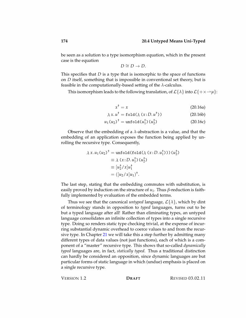
174 20.4 Untyped Means Uni-Typed
be seen as a solution to a type isomorphism equation, which in the presentcase is the equation
D I= D 3 D.
This specifies that D is a type that is isomorphic to the space of functionson D itself, something that is impossible in conventional set theory, but isfeasible in the computationally-based setting of the !-calculus.
This isomorphism leads to the following translation, of L{!} into L{+<"µ}:
x† = x (20.16a)
! x. u† = fold(! (x:D. u†)) (20.16b)
u1(u2)† = unfold(u†
1)(u†2) (20.16c)
Observe that the embedding of a !-abstraction is a value, and that theembedding of an application exposes the function being applied by un-rolling the recursive type. Consequently,
! x. u1(u2)† = unfold(fold(! (x:D. u†
1)))(u†2)
9 ! (x:D. u†1)(u†
2)
9 [u†2/x]u†
1
= ([u2/x]u1)†.
The last step, stating that the embedding commutes with substitution, iseasily proved by induction on the structure of u1. Thus --reduction is faith-fully implemented by evaluation of the embedded terms.
Thus we see that the canonical untyped language, L{!}, which by dintof terminology stands in opposition to typed languages, turns out to bebut a typed language after all! Rather than eliminating types, an untypedlanguage consolidates an infinite collection of types into a single recursivetype. Doing so renders static type checking trivial, at the expense of incur-ring substantial dynamic overhead to coerce values to and from the recur-sive type. In Chapter 21 we will take this a step further by admitting manydifferent types of data values (not just functions), each of which is a com-ponent of a “master” recursive type. This shows that so-called dynamicallytyped languages are, in fact, statically typed. Thus a traditional distinctioncan hardly be considered an opposition, since dynamic languages are butparticular forms of static language in which (undue) emphasis is placed ona single recursive type.
VERSION 1.2 DRAFT REVISED 03.02.11
20.5 Exercises 175
20.5 Exercises
REVISED 03.02.11 DRAFT VERSION 1.2

176 20.5 Exercises
VERSION 1.2 DRAFT REVISED 03.02.11
Chapter 21
Dynamic Typing
We saw in Chapter 20 that an untyped language may be viewed as a uni-typed language in which the so-called untyped terms are terms of a distin-guished recursive type. In the case of the untyped !-calculus this recursivetype has a particularly simple form, expressing that every term is isomor-phic to a function. Consequently, no run-time errors can occur due to themisuse of a value—the only elimination form is application, and its first ar-gument can only be a function. Obviously this property breaks down oncemore than one class of value is permitted into the language. For example, ifwe add natural numbers as a primitive concept to the untyped !-calculus(rather than defining them via Church encodings), then it is possible to in-cur a run-time error arising from attempting to apply a number to an argu-ment, or to add a function to a number. One school of thought in languagedesign is to turn this vice into a virtue by embracing a model of compu-tation that has multiple classes of value of a single type. Such languagesare said to be dynamically typed, in purported opposition to statically typedlanguages. But the supposed opposition is illusory. Just as the untyped !-calculus is really unityped, so dynamic languages are special cases of staticlanguages.
21.1 Dynamically Typed PCF
To illustrate dynamic typing we formulate a dynamically typed version ofL{nat"}, called L{dyn}. The abstract syntax of L{dyn} is given by the
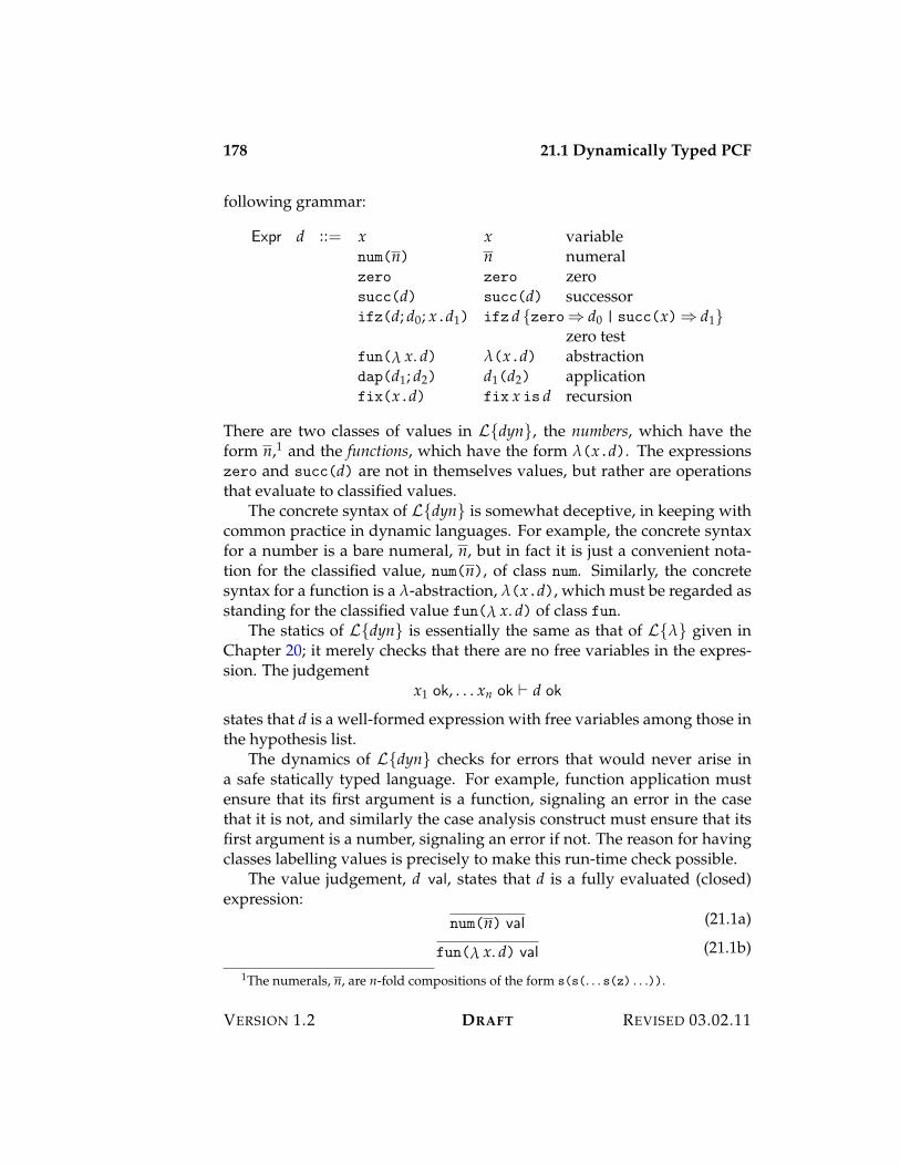
178 21.1 Dynamically Typed PCF
following grammar:
Expr d ::= x x variablenum(n) n numeralzero zero zerosucc(d) succ(d) successorifz(d; d0; x.d1) ifz d {zero; d0 | succ(x); d1}
zero testfun(! x. d) !(x.d) abstractiondap(d1; d2) d1(d2) applicationfix(x.d) fix x is d recursion
There are two classes of values in L{dyn}, the numbers, which have theform n,1 and the functions, which have the form !(x.d). The expressionszero and succ(d) are not in themselves values, but rather are operationsthat evaluate to classified values.
The concrete syntax of L{dyn} is somewhat deceptive, in keeping withcommon practice in dynamic languages. For example, the concrete syntaxfor a number is a bare numeral, n, but in fact it is just a convenient nota-tion for the classified value, num(n), of class num. Similarly, the concretesyntax for a function is a !-abstraction, !(x.d), which must be regarded asstanding for the classified value fun(! x. d) of class fun.
The statics of L{dyn} is essentially the same as that of L{!} given inChapter 20; it merely checks that there are no free variables in the expres-sion. The judgement
x1 ok, . . . xn ok ) d ok
states that d is a well-formed expression with free variables among those inthe hypothesis list.
The dynamics of L{dyn} checks for errors that would never arise ina safe statically typed language. For example, function application mustensure that its first argument is a function, signaling an error in the casethat it is not, and similarly the case analysis construct must ensure that itsfirst argument is a number, signaling an error if not. The reason for havingclasses labelling values is precisely to make this run-time check possible.
The value judgement, d val, states that d is a fully evaluated (closed)expression:
num(n) val (21.1a)
fun(! x. d) val (21.1b)
1The numerals, n, are n-fold compositions of the form s(s(. . . s(z) . . .)).
VERSION 1.2 DRAFT REVISED 03.02.11
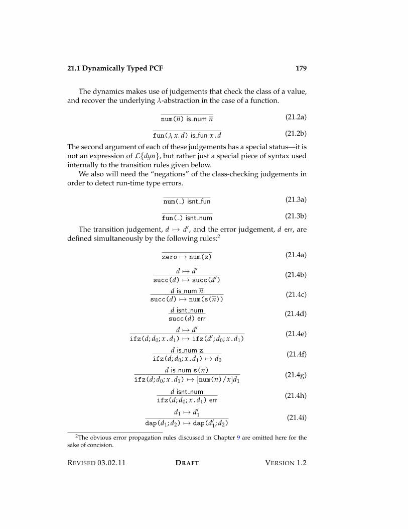
21.1 Dynamically Typed PCF 179
The dynamics makes use of judgements that check the class of a value,and recover the underlying !-abstraction in the case of a function.
num(n) is num n (21.2a)
fun(! x. d) is fun x.d (21.2b)
The second argument of each of these judgements has a special status—it isnot an expression of L{dyn}, but rather just a special piece of syntax usedinternally to the transition rules given below.
We also will need the “negations” of the class-checking judgements inorder to detect run-time type errors.
num( ) isnt fun (21.3a)
fun( ) isnt num (21.3b)
The transition judgement, d 53 d%, and the error judgement, d err, aredefined simultaneously by the following rules:2
zero 53 num(z) (21.4a)
d 53 d%succ(d) 53 succ(d%)
(21.4b)
d is num nsucc(d) 53 num(s(n)) (21.4c)
d isnt numsucc(d) err
(21.4d)
d 53 d%ifz(d; d0; x.d1) 53 ifz(d%; d0; x.d1)
(21.4e)
d is num zifz(d; d0; x.d1) 53 d0
(21.4f)
d is num s(n)ifz(d; d0; x.d1) 53 [num(n)/x]d1
(21.4g)
d isnt numifz(d; d0; x.d1) err
(21.4h)
d1 53 d%1dap(d1; d2) 53 dap(d%1; d2)
(21.4i)
2The obvious error propagation rules discussed in Chapter 9 are omitted here for thesake of concision.
REVISED 03.02.11 DRAFT VERSION 1.2
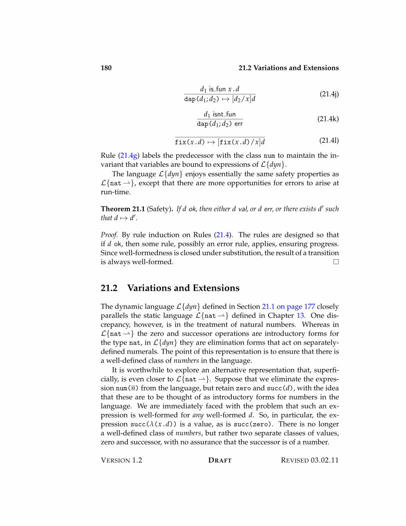
180 21.2 Variations and Extensions
d1 is fun x.ddap(d1; d2) 53 [d2/x]d
(21.4j)
d1 isnt fundap(d1; d2) err
(21.4k)
fix(x.d) 53 [fix(x.d)/x]d (21.4l)
Rule (21.4g) labels the predecessor with the class num to maintain the in-variant that variables are bound to expressions of L{dyn}.
The language L{dyn} enjoys essentially the same safety properties asL{nat"}, except that there are more opportunities for errors to arise atrun-time.
Theorem 21.1 (Safety). If d ok, then either d val, or d err, or there exists d% suchthat d 53 d%.
Proof. By rule induction on Rules (21.4). The rules are designed so thatif d ok, then some rule, possibly an error rule, applies, ensuring progress.Since well-formedness is closed under substitution, the result of a transitionis always well-formed.
21.2 Variations and Extensions
The dynamic language L{dyn} defined in Section 21.1 on page 177 closelyparallels the static language L{nat"} defined in Chapter 13. One dis-crepancy, however, is in the treatment of natural numbers. Whereas inL{nat"} the zero and successor operations are introductory forms forthe type nat, in L{dyn} they are elimination forms that act on separately-defined numerals. The point of this representation is to ensure that there isa well-defined class of numbers in the language.
It is worthwhile to explore an alternative representation that, superfi-cially, is even closer to L{nat"}. Suppose that we eliminate the expres-sion num(n) from the language, but retain zero and succ(d), with the ideathat these are to be thought of as introductory forms for numbers in thelanguage. We are immediately faced with the problem that such an ex-pression is well-formed for any well-formed d. So, in particular, the ex-pression succ(!(x.d)) is a value, as is succ(zero). There is no longera well-defined class of numbers, but rather two separate classes of values,zero and successor, with no assurance that the successor is of a number.
VERSION 1.2 DRAFT REVISED 03.02.11
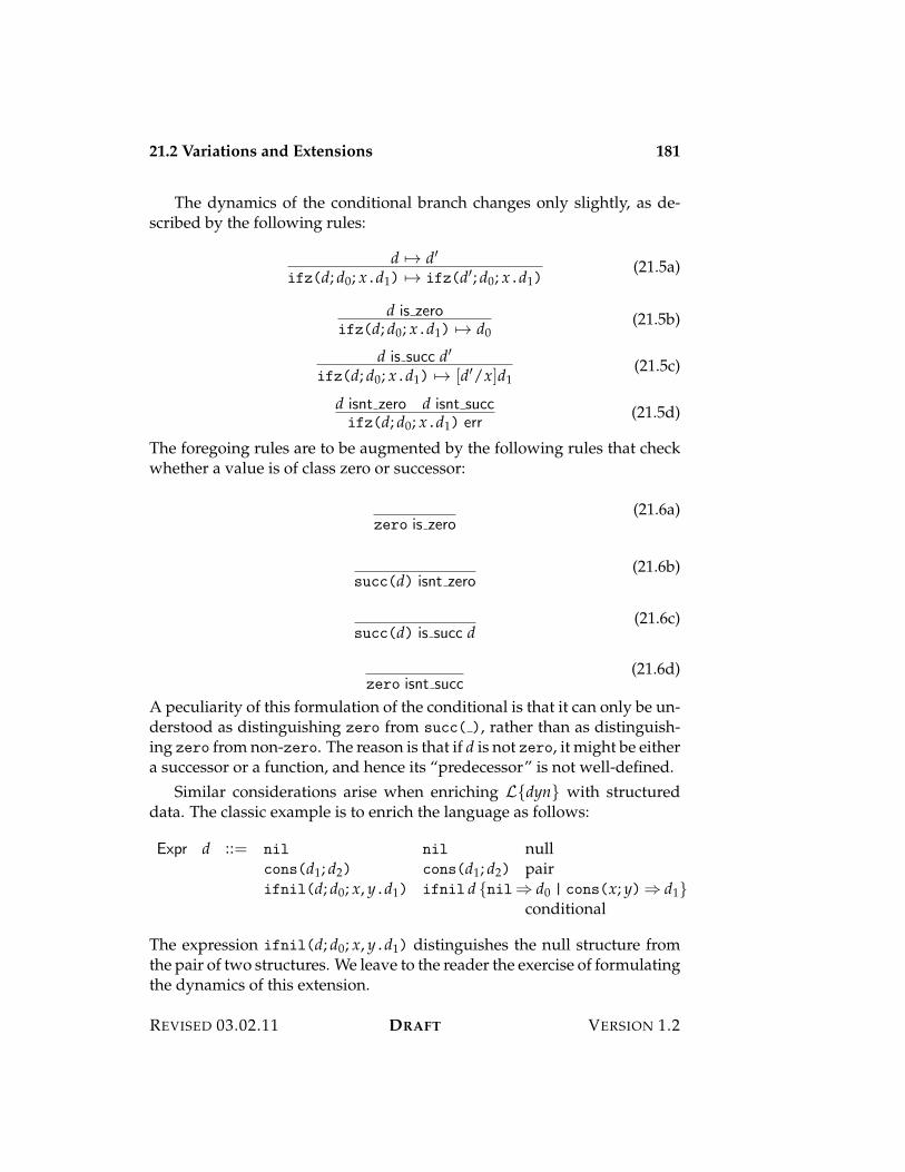
21.2 Variations and Extensions 181
The dynamics of the conditional branch changes only slightly, as de-scribed by the following rules:
d 53 d%ifz(d; d0; x.d1) 53 ifz(d%; d0; x.d1)
(21.5a)
d is zeroifz(d; d0; x.d1) 53 d0
(21.5b)
d is succ d%ifz(d; d0; x.d1) 53 [d%/x]d1
(21.5c)
d isnt zero d isnt succifz(d; d0; x.d1) err
(21.5d)
The foregoing rules are to be augmented by the following rules that checkwhether a value is of class zero or successor:
zero is zero(21.6a)
succ(d) isnt zero(21.6b)
succ(d) is succ d(21.6c)
zero isnt succ(21.6d)
A peculiarity of this formulation of the conditional is that it can only be un-derstood as distinguishing zero from succ( ), rather than as distinguish-ing zero from non-zero. The reason is that if d is not zero, it might be eithera successor or a function, and hence its “predecessor” is not well-defined.
Similar considerations arise when enriching L{dyn} with structureddata. The classic example is to enrich the language as follows:
Expr d ::= nil nil nullcons(d1; d2) cons(d1; d2) pairifnil(d; d0; x, y.d1) ifnil d {nil; d0 | cons(x; y); d1}
conditional
The expression ifnil(d; d0; x, y.d1) distinguishes the null structure fromthe pair of two structures. We leave to the reader the exercise of formulatingthe dynamics of this extension.
REVISED 03.02.11 DRAFT VERSION 1.2
182 21.2 Variations and Extensions
An advantage of dynamic typing is that the constructors nil and cons(d1; d2)
are sufficient to build unbounded, as well as bounded, data structures suchas lists or trees. For example, the list consisting of three zero’s may be rep-resented by the value
cons(zero; cons(zero; cons(zero; nil))).
But what to make of this beast?
cons(zero; cons(zero; cons(zero; !(x)x))).
It is a perfectly valid expression, but does not correspond to any naturaldata structure.
The disadvantage of this representation becomes apparent as soon asone wishes to define operations on lists, such as the append function:
fix a is!(x.!(y.ifnil(x; y; x1, x2.cons(x1; a(x2)(y)))))
What if x is the second list-like value given above? As it stands, the ap-pend function will signal an error upon reaching the function at the end ofthe list. If, however, y is this value, no error is signalled. This asymmetrymay seem innocuous, but it is only one simple manifestation of a perva-sive problem with dynamic languages: it is impossible to state within thelanguage even the most rudimentary assumptions about the inputs, suchas the assumption that both arguments to the append function ought to begenuine lists.
The conditional expression ifnil(d; d0; x, y.d1) is rather ad hoc in thatit makes a distinction between nil and all other values. Why not distin-guish successors from non-succcessors, or functions from non-functions?A more systematic approach is to enrich the language with predicates anddestructors. Predicates determine whether a value is of a specified class, anddestructors recover the value labelled with a given class.
Expr d ::= cond(d; d0; d1) cond(d; d0; d1) conditionalnil?(d) nil?(d) nil testcons?(d) cons?(d) pair testcar(d) car(d) first projectioncdr(d) cdr(d) second projection
The conditional cond(d; d0; d1) distinguishes d between nil and all othervalues. If d is not nil, the conditional evaluates to d0, and otherwise eval-uates to d1. In other words the value nil represents boolean falsehood,
VERSION 1.2 DRAFT REVISED 03.02.11
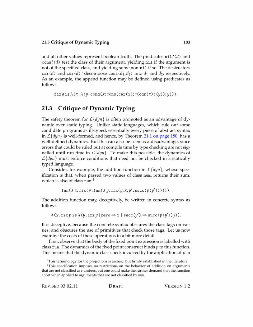
21.3 Critique of Dynamic Typing 183
and all other values represent boolean truth. The predicates nil?(d) andcons?(d) test the class of their argument, yielding nil if the argument isnot of the specified class, and yielding some non-nil if so. The destructorscar(d) and cdr(d)3 decompose cons(d1; d2) into d1 and d2, respectively.As an example, the append function may be defined using predicates asfollows:
fix a is!(x.!(y.cond(x; cons(car(x); a(cdr(x))(y)); y))).
21.3 Critique of Dynamic Typing
The safety theorem for L{dyn} is often promoted as an advantage of dy-namic over static typing. Unlike static languages, which rule out somecandidate programs as ill-typed, essentially every piece of abstract syntaxin L{dyn} is well-formed, and hence, by Theorem 21.1 on page 180, has awell-defined dynamics. But this can also be seen as a disadvantage, sinceerrors that could be ruled out at compile time by type checking are not sig-nalled until run time in L{dyn}. To make this possible, the dynamics ofL{dyn} must enforce conditions that need not be checked in a staticallytyped language.
Consider, for example, the addition function in L{dyn}, whose spec-ification is that, when passed two values of class num, returns their sum,which is also of class num:4
fun(! x. fix(p.fun(! y. ifz(y; x; y%.succ(p(y%)))))).
The addition function may, deceptively, be written in concrete syntax asfollows:
!(x.fix p is!(y.ifz y {zero; x | succ(y%); succ(p(y%))})).
It is deceptive, because the concrete syntax obscures the class tags on val-ues, and obscures the use of primitives that check those tags. Let us nowexamine the costs of these operations in a bit more detail.
First, observe that the body of the fixed point expression is labelled withclass fun. The dynamics of the fixed point construct binds p to this function.This means that the dynamic class check incurred by the application of p in
3This terminology for the projections is archaic, but firmly established in the literature.4This specification imposes no restrictions on the behavior of addition on arguments
that are not classified as numbers, but one could make the further demand that the functionabort when applied to arguments that are not classified by num.
REVISED 03.02.11 DRAFT VERSION 1.2
184 21.4 Exercises
the recursive call is guaranteed to succeed. But L{dyn} offers no means ofsuppressing this redundant check, because it cannot express the invariantthat p is always bound to a value of class fun.
Second, observe that the result of applying the inner !-abstraction iseither x, the argument of the outer !-abstraction, or the successor of a re-cursive call to the function itself. The successor operation checks that itsargument is of class num, even though this is guaranteed for all but thebase case, which returns the given x, which can be of any class at all. Inprinciple we can check that x is of class num once, and observe that it is oth-erwise a loop invariant that the result of applying the inner function is ofthis class. However, L{dyn} gives us no way to express this invariant; therepeated, redundant tag checks imposed by the successor operation cannotbe avoided.
Third, the argument, y, to the inner function is either the original ar-gument to the addition function, or is the predecessor of some earlier re-cursive call. But as long as the original call is to a value of class num, thenthe dynamics of the conditional will ensure that all recursive calls have thisclass. And again there is no way to express this invariant in L{dyn}, andhence there is no way to avoid the class check imposed by the conditionalbranch.
Classification is not free—storage is required for the class label, and ittakes time to detach the class from a value each time it is used and to attacha class to a value whenever it is created. Although the overhead of classi-fication is not asymptotically significant (it slows down the program onlyby a constant factor), it is nevertheless non-negligible, and should be elim-inated whenever possible. But this is impossible within L{dyn}, because itcannot enforce the restrictions required to express the required invariants.For that we need a static type system.
21.4 Exercises
VERSION 1.2 DRAFT REVISED 03.02.11
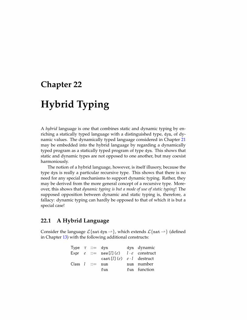
Chapter 22
Hybrid Typing
A hybrid language is one that combines static and dynamic typing by en-riching a statically typed language with a distinguished type, dyn, of dy-namic values. The dynamically typed language considered in Chapter 21may be embedded into the hybrid language by regarding a dynamicallytyped program as a statically typed program of type dyn. This shows thatstatic and dynamic types are not opposed to one another, but may coexistharmoniously.
The notion of a hybrid language, however, is itself illusory, because thetype dyn is really a particular recursive type. This shows that there is noneed for any special mechanisms to support dynamic typing. Rather, theymay be derived from the more general concept of a recursive type. More-over, this shows that dynamic typing is but a mode of use of static typing! Thesupposed opposition between dynamic and static typing is, therefore, afallacy: dynamic typing can hardly be opposed to that of which it is but aspecial case!
22.1 A Hybrid Language
Consider the language L{nat dyn"}, which extends L{nat"} (definedin Chapter 13) with the following additional constructs:
Type " ::= dyn dyn dynamicExpr e ::= new[l](e) l · e construct
cast[l](e) e · l destructClass l ::= num num number
fun fun function
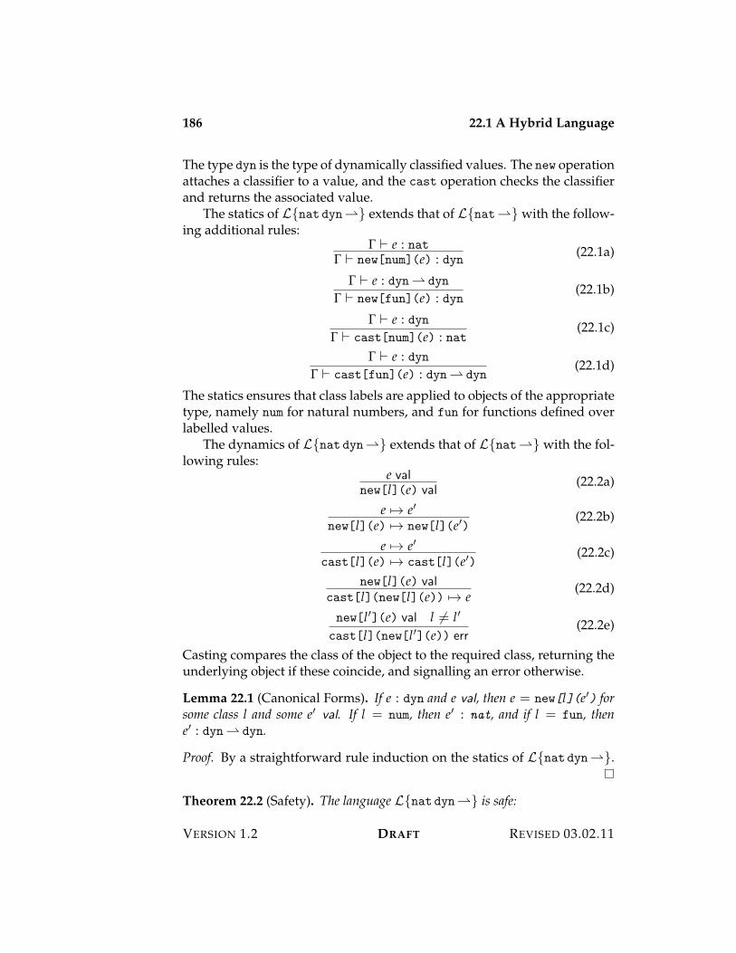
186 22.1 A Hybrid Language
The type dyn is the type of dynamically classified values. The new operationattaches a classifier to a value, and the cast operation checks the classifierand returns the associated value.
The statics of L{nat dyn"} extends that of L{nat"} with the follow-ing additional rules:
! ) e : nat! ) new[num](e) : dyn (22.1a)
! ) e : dyn" dyn
! ) new[fun](e) : dyn(22.1b)
! ) e : dyn! ) cast[num](e) : nat
(22.1c)
! ) e : dyn! ) cast[fun](e) : dyn" dyn
(22.1d)
The statics ensures that class labels are applied to objects of the appropriatetype, namely num for natural numbers, and fun for functions defined overlabelled values.
The dynamics of L{nat dyn"} extends that of L{nat"} with the fol-lowing rules:
e valnew[l](e) val
(22.2a)
e 53 e%new[l](e) 53 new[l](e%)
(22.2b)
e 53 e%cast[l](e) 53 cast[l](e%)
(22.2c)
new[l](e) valcast[l](new[l](e)) 53 e
(22.2d)
new[l%](e) val l ,= l%
cast[l](new[l%](e)) err(22.2e)
Casting compares the class of the object to the required class, returning theunderlying object if these coincide, and signalling an error otherwise.
Lemma 22.1 (Canonical Forms). If e : dyn and e val, then e = new[l](e%) forsome class l and some e% val. If l = num, then e% : nat, and if l = fun, thene% : dyn" dyn.
Proof. By a straightforward rule induction on the statics of L{nat dyn"}.
Theorem 22.2 (Safety). The language L{nat dyn"} is safe:
VERSION 1.2 DRAFT REVISED 03.02.11
22.2 Optimization of Dynamic Typing 187
1. If e : " and e 53 e%, then e% : ".
2. If e : ", then either e val, or e err, or e 53 e% for some e%.
Proof. Preservation is proved by rule induction on the dynamics, and progressis proved by rule induction on the statics, making use of the canonicalforms lemma. The opportunities for run-time errors are the same as thosefor L{dyn}—a well-typed cast might fail at run-time if the class of the castdoes not match the class of the value.
22.2 Optimization of Dynamic Typing
The language L{nat dyn"} combines static and dynamic typing by en-riching L{nat"} with the type, dyn, of classified values. It is, for thisreason, called a hybrid language. Unlike a purely dynamic type system, ahybrid type system can express invariants that are crucial to the optimiza-tion of programs in L{dyn}.
Let us examine this in the case of the addition function, which may bedefined in L{nat dyn"} as follows:
fun · ! (x:dyn. fix p:dyn is fun · ! (y:dyn. ex,p,y)),
wherex : dyn, p : dyn, y : dyn ) ex,p,y : dyn
is defined to be the expression
ifz (y · num) {zero; x | succ(y%); num · (s((p · fun)(num · y%) · num))}.
This is a reformulation of the dynamic addition function given in Section 21.3on page 183 in which we have made explicit the checking and imposition ofclasses on values. We will exploit the static type system of L{nat dyn"} tooptimize this dynamically typed implementation of addition in accordancewith the specification given in Section 21.3 on page 183.
First, note that the body of the fix expression is an explicitly labelledfunction. This means that when the recursion is unwound, the variable p isbound to this value of type dyn. Consequently, the check that p is labelledwith class fun is redundant, and can be eliminated. This is achieved byrewriting the function as follows:
fun · ! (x:dyn. fun · fix p:dyn" dyn is! (y:dyn. e%x,p,y)),
REVISED 03.02.11 DRAFT VERSION 1.2
188 22.2 Optimization of Dynamic Typing
where e%x,p,y is the expression
ifz (y · num) {zero; x | succ(y%); num · (s(p(num · y%) · num))}.
We have “hoisted” the function class label out of the loop, and suppressedthe cast inside the loop. Correspondingly, the type of p has changed todyn" dyn, reflecting that the body is now a “bare function”, rather than alabelled function value of type dyn.
Next, observe that the parameter y of type dyn is cast to a number oneach iteration of the loop before it is tested for zero. Since this functionis recursive, the bindings of y arise in one of two ways, at the initial callto the addition function, and on each recursive call. But the recursive callis made on the predecessor of y, which is a true natural number that islabelled with num at the call site, only to be removed by the class check atthe conditional on the next iteration. This suggests that we hoist the checkon y outside of the loop, and avoid labelling the argument to the recursivecall. Doing so changes the type of the function, however, from dyn" dyn tonat" dyn. Consequently, further changes are required to ensure that theentire function remains well-typed.
Before doing so, let us make another observation. The result of the re-cursive call is checked to ensure that it has class num, and, if so, the un-derlying value is incremented and labelled with class num. If the resultof the recursive call came from an earlier use of this branch of the condi-tional, then obviously the class check is redundant, because we know thatit must have class num. But what if the result came from the other branch ofthe conditional? In that case the function returns x, which need not be ofclass num because it is provided by the caller of the function. However, wemay reasonably insist that it is an error to call addition with a non-numericargument. This canbe enforced by replacing x in the zero branch of theconditional by x · num.
Combining these optimizations we obtain the inner loop e%%x defined asfollows:
fix p:nat" nat is! (y:nat. ifz y {zero; x · num | succ(y%); s(p(y%))}).
This function has type nat" nat, and runs at full speed when applied to anatural number—all checks have been hoisted out of the inner loop.
Finally, recall that the overall goal is to define a version of addition thatworks on values of type dyn. Thus we require a value of type dyn" dyn,but what we have at hand is a function of type nat" nat. This can be
VERSION 1.2 DRAFT REVISED 03.02.11
22.3 Static “Versus” Dynamic Typing 189
converted to the required form by pre-composing with a cast to num andpost-composing with a coercion to num:
fun · ! (x:dyn. fun · ! (y:dyn. num · (e%%x(y · num)))).
The innermost !-abstraction converts the function e%%x from type nat" nat
to type dyn" dyn by composing it with a class check that ensures that y isa natural number at the initial call site, and applies a label to the result torestore it to type dyn.
22.3 Static “Versus” Dynamic Typing
There are many attempts to distinguish dynamic from static typing, all ofwhich are misleading or wrong. For example, it is often said that static typesystems associate types with variables, but dynamic type systems associatetypes with values. This oft-repeated characterization appears to be justifiedby the absence of type annotations on !-abstractions, and the presence ofclasses on values. But it is based on a confusion of classes with types—theclass of a value (num or fun) is not its type. Moreover, a static type system as-signs types to values just as surely as it does to variables, so the descriptionfails on this account as well.
Another way to differentiate dynamic from static languages is to saythat whereas static languages check types at compile time, dynamic lan-guages check types at run time. But to say that static languages check typesstatically is to state a tautology, and to say that dynamic languages checktypes at run-time is to utter a falsehood. Dynamic languages perform classchecking, not type checking, at run-time. For example, application checks thatits first argument is labelled with fun; it does not type check the body ofthe function. Indeed, at no point does the dynamics compute the type of avalue, rather it checks its class against its expectations before proceeding.Here again, a supposed contrast between static and dynamic languagesevaporates under careful analysis.
Another characterization is to assert that dynamic languages admit het-erogeneous collections, whereas static languages admit only homogeneouscollections. For example, in a dynamic language the elements of a list maybe of disparate classes, as illustrated by the expression
cons(s(z); cons(!(!(x.x)); nil)).
But they are nevertheless all of the same type! Put the other way around,a static language with a dynamic type is just as capable of representing aheterogeneous collection as is a dynamic language with only one type.
REVISED 03.02.11 DRAFT VERSION 1.2
190 22.4 Reduction to Recursive Types
What, then, are we to make of the traditional distinction between dy-namic and static languages? Rather than being in opposition to each other,we see that dynamic languages are a mode of use of static languages. If we havea type dyn in the language, then we have all of the apparatus of dynamiclanguages at our disposal, so there is no loss of expressive power. But thereis a very significant gain from embedding dynamic typing within a statictype discipline! We can avoid much of the overhead of dynamic typing bysimply limiting our use of the type dyn in our programs, as was illustratedin Section 22.2 on page 187.
22.4 Reduction to Recursive Types
The type dyn codifies the use of dynamic typing within a static language. Itsintroduction form labels an object of the appropriate type, and its elimina-tion form is a (possibly undefined) casting operation. Rather than treatingdyn as primitive, we may derive it as a particular use of recursive types,according to the following definitions:
dyn = µt.[num : nat, fun : t " t] (22.3)new[num](e) = fold(num · e) (22.4)new[fun](e) = fold(fun · e) (22.5)cast[num](e) = case unfold(e) {num · x ; x | fun · x ; error} (22.6)cast[fun](e) = case unfold(e) {num · x ; error | fun · x ; x} (22.7)
One may readily check that the static and dynamics for the type dyn arederivable according to these definitions.
This encoding readily generalizes to any number of classes of values:we need only consider additional summands corresponding to each class.For example, to account for the constructors nil and cons(d1; d2) consid-ered in Chapter 21, the definition of dyn is expanded to the recursive type
µt.[num : nat, fun : t " t, nil : unit, cons : t < t],
with corresponding definitions for the new and cast operations. This ex-emplifies the general case: dynamic typing is a mode of use of static typesin which classes of values are simply names of summands in a recursivetype of dynamic values.
VERSION 1.2 DRAFT REVISED 03.02.11

Part VIII
Variable Types

Chapter 23
Girard’s System F
The languages we have considered so far are all monomorphic in that everyexpression has a unique type, given the types of its free variables, if it hasa type at all. Yet it is often the case that essentially the same behavior is re-quired, albeit at several different types. For example, in L{nat3} there isa distinct identity function for each type ", namely ! (x:". x), even thoughthe behavior is the same for each choice of ". Similarly, there is a distinctcomposition operator for each triple of types, namely
8"1,"2,"3 = ! ( f:"2 3 "3. ! (g:"1 3 "2. ! (x:"1. f(g(x))))).
Each choice of the three types requires a different program, even thoughthey all exhibit the same behavior when executed.
Obviously it would be useful to capture the general pattern once andfor all, and to instantiate this pattern each time we need it. The expressionpatterns codify generic (type-independent) behaviors that are shared by allinstances of the pattern. Such generic expressions are said to be polymor-phic. In this chapter we will study a language introduced by Girard underthe name System F and by Reynolds under the name polymorphic typed !-calculus. Although motivated by a simple practical problem (how to avoidwriting redundant code), the concept of polymorphism is central to an im-pressive variety of seemingly disparate concepts, including the concept ofdata abstraction (the subject of Chapter 24), and the definability of product,sum, inductive, and coinductive types considered in the preceding chap-ters. (Only general recursive types extend the expressive power of the lan-guage.)
194 23.1 System F
23.1 System F
System F, or the polymorphic !-calculus, or L{3&}, is a minimal functionallanguage that illustrates the core concepts of polymorphic typing, and per-mits us to examine its surprising expressive power in isolation from otherlanguage features. The syntax of System F is given by the following gram-mar:
Type " ::= t t variablearr("1; "2) "1 3 "2 functionall(t.") &(t.") polymorphic
Expr e ::= x xlam["](x.e) ! (x:". e) abstractionap(e1; e2) e1(e2) applicationLam(t.e) ((t.e) type abstractionApp["](e) e["] type application
A type abstraction, Lam(t.e), defines a generic, or polymorphic, function withtype parameter t standing for an unspecified type within e. A type application,or instantiation, App["](e), applies a polymorphic function to a specifiedtype, which is then plugged in for the type parameter to obtain the result.Polymorphic functions are classified by the universal type, all(t."), thatdetermines the type, ", of the result as a function of the argument, t.
The statics of L{3&} consists of two judgement forms, the type forma-tion judgement,
!t | " ) " type,
and the typing judgement,
!t !x | " ! ) e : ".
These are generic judgements over type variables !t and expression variables!x. They are also hypothetical in a set " of type assumptions of the formt type, where t + T , and typing assumptions of the form x : ", where x + Tand " ) " type. As usual we drop explicit mention of the parameter sets,relying on typographical conventions to determine them.
The rules defining the type formation judgement are as follows:
", t type ) t type (23.1a)
" ) "1 type " ) "2 type" ) arr("1; "2) type
(23.1b)
VERSION 1.2 DRAFT REVISED 03.02.11
23.1 System F 195
", t type ) " type" ) all(t.") type
(23.1c)
The rules defining the typing judgement are as follows:
" !, x : " ) x : " (23.2a)
" ) "1 type " !, x : "1 ) e : "2" ! ) lam["1](x.e) : arr("1; "2)
(23.2b)
" ! ) e1 : arr("2; ") " ! ) e2 : "2" ! ) ap(e1; e2) : "
(23.2c)
", t type ! ) e : "" ! ) Lam(t.e) : all(t.")
(23.2d)
" ! ) e : all(t."%) " ) " type
" ! ) App["](e) : ["/t]"% (23.2e)
Lemma 23.1 (Regularity). If " ! ) e : ", and if " ) "i type for each assumptionxi : "i in !, then " ) " type.
Proof. By induction on Rules (23.2).
The statics admits the structural rules for a general hypothetical judge-ment. In particular, we have the following critical substitution property fortype formation and expression typing.
Lemma 23.2 (Substitution). 1. If ", t type ) "% type and " ) " type, then" ) ["/t]"% type.
2. If ", t type ! ) e% : "% and " ) " type, then " ["/t]! ) ["/t]e% : ["/t]"%.
3. If " !, x : " ) e% : "% and " ! ) e : ", then " ! ) [e/x]e% : "%.
The second part of the lemma requires substitution into the context, !,as well as into the term and its type, because the type variable t may occurfreely in any of these positions.
Returning to the motivating examples from the introduction, the poly-morphic identity function, I, is written
((t.! (x:t. x));
it has the polymorphic type
&(t.t 3 t).
REVISED 03.02.11 DRAFT VERSION 1.2
196 23.1 System F
Instances of the polymorphic identity are written I["], where " is sometype, and have the type " 3 ".
Similarly, the polymorphic composition function, C, is written
((t1.((t2.((t3.! ( f:t2 3 t3. ! (g:t1 3 t2. ! (x:t1. f(g(x)))))))).
The function C has the polymorphic type
&(t1.&(t2.&(t3.(t2 3 t3) 3 (t1 3 t2) 3 (t1 3 t3)))).
Instances of C are obtained by applying it to a triple of types, writingC["1]["2]["3]. Each such instance has the type
("2 3 "3) 3 ("1 3 "2) 3 ("1 3 "3).
Dynamics
The dynamics of L{3&} is given as follows:
lam["](x.e) val (23.3a)
Lam(t.e) val (23.3b)
ap(lam["1](x.e); e2) 53 [e2/x]e (23.3c)
e1 53 e%1ap(e1; e2) 53 ap(e%1; e2)
(23.3d)
App["](Lam(t.e)) 53 ["/t]e (23.3e)
e 53 e%App["](e) 53 App["](e%) (23.3f)
These rules endow L{3&} with a call-by-name interpretation of applica-tion, but one could as well consider a call-by-value variant.
It is a simple matter to prove safety for L{3&}, using familiar methods.
Lemma 23.3 (Canonical Forms). Suppose that e : " and e val, then
1. If " = arr("1; "2), then e = lam["1](x.e2) with x : "1 ) e2 : "2.
2. If " = all(t."%), then e = Lam(t.e%) with t type ) e% : "%.
Proof. By rule induction on the statics.
Theorem 23.4 (Preservation). If e : & and e 53 e%, then e% : &.
VERSION 1.2 DRAFT REVISED 03.02.11
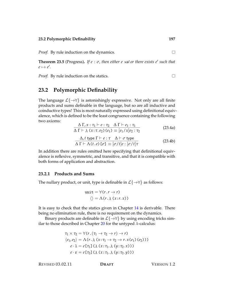
23.2 Polymorphic Definability 197
Proof. By rule induction on the dynamics.
Theorem 23.5 (Progress). If e : &, then either e val or there exists e% such thate 53 e%.
Proof. By rule induction on the statics.
23.2 Polymorphic Definability
The language L{3&} is astonishingly expressive. Not only are all finiteproducts and sums definable in the language, but so are all inductive andcoinductive types! This is most naturally expressed using definitional equiv-alence, which is defined to be the least congruence containing the followingtwo axioms:
" !, x : "1 ) e : "2 " ! ) e1 : "1
" ! ) ! (x:". e2)(e1) 9 [e1/x]e2 : "2(23.4a)
", t type ! ) e : " " ) & type
" ! ) ((t.e)[&] 9 [&/t]e : [&/t]"(23.4b)
In addition there are rules omitted here specifying that definitional equiv-alence is reflexive, symmetric, and transitive, and that it is compatible withboth forms of application and abstraction.
23.2.1 Products and Sums
The nullary product, or unit, type is definable in L{3&} as follows:
unit = &(r.r 3 r)?@ = ((r.! (x:r. x))
It is easy to check that the statics given in Chapter 14 is derivable. Therebeing no elimination rule, there is no requirement on the dynamics.
Binary products are definable in L{3&} by using encoding tricks sim-ilar to those described in Chapter 20 for the untyped !-calculus:
"1 < "2 = &(r.("1 3 "2 3 r) 3 r)?e1, e2@ = ((r.! (x:"1 3 "2 3 r. x(e1)(e2)))
e · l = e["1](! (x:"1. ! (y:"2. x)))e · r = e["2](! (x:"1. ! (y:"2. y)))
REVISED 03.02.11 DRAFT VERSION 1.2
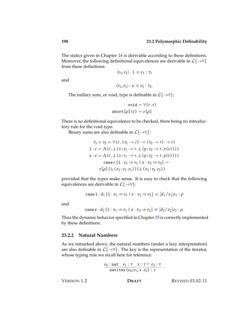
198 23.2 Polymorphic Definability
The statics given in Chapter 14 is derivable according to these definitions.Moreover, the following definitional equivalences are derivable in L{3&}from these definitions:
?e1, e2@ · l 9 e1 : "1
and?e1, e2@ · r 9 e2 : "2.
The nullary sum, or void, type is definable in L{3&}:
void = &(r.r)abort[,](e) = e[,]
There is no definitional equivalence to be checked, there being no introduc-tory rule for the void type.
Binary sums are also definable in L{3&}:
"1 + "2 = &(r.("1 3 r) 3 ("2 3 r) 3 r)l · e = ((r.! (x:"1 3 r. ! (y:"2 3 r. x(e))))r · e = ((r.! (x:"1 3 r. ! (y:"2 3 r. y(e))))
case e {l · x1 ; e1 | r · x2 ; e2} =
e[,](! (x1:"1. e1))(! (x2:"2. e2))
provided that the types make sense. It is easy to check that the followingequivalences are derivable in L{3&}:
case l · d1 {l · x1 ; e1 | r · x2 ; e2} 9 [d1/x1]e1 : ,
andcase r · d2 {l · x1 ; e1 | r · x2 ; e2} 9 [d2/x2]e2 : ,.
Thus the dynamic behavior specified in Chapter 15 is correctly implementedby these definitions.
23.2.2 Natural Numbers
As we remarked above, the natural numbers (under a lazy interpretation)are also definable in L{3&}. The key is the representation of the iterator,whose typing rule we recall here for reference:
e0 : nat e1 : " x : " ) e2 : "natiter(e0; e1; x.e2) : "
.
VERSION 1.2 DRAFT REVISED 03.02.11
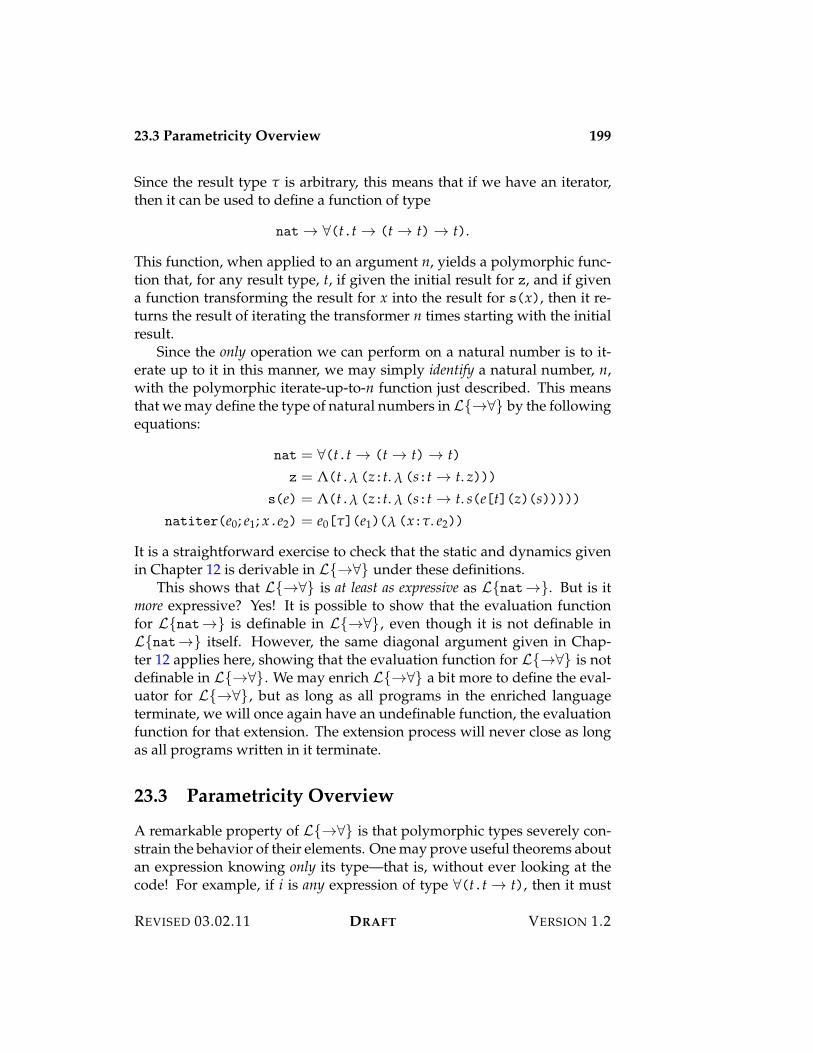
23.3 Parametricity Overview 199
Since the result type " is arbitrary, this means that if we have an iterator,then it can be used to define a function of type
nat 3 &(t.t 3 (t 3 t) 3 t).
This function, when applied to an argument n, yields a polymorphic func-tion that, for any result type, t, if given the initial result for z, and if givena function transforming the result for x into the result for s(x), then it re-turns the result of iterating the transformer n times starting with the initialresult.
Since the only operation we can perform on a natural number is to it-erate up to it in this manner, we may simply identify a natural number, n,with the polymorphic iterate-up-to-n function just described. This meansthat we may define the type of natural numbers in L{3&} by the followingequations:
nat = &(t.t 3 (t 3 t) 3 t)z = ((t.! (z:t. ! (s:t 3 t. z)))
s(e) = ((t.! (z:t. ! (s:t 3 t. s(e[t](z)(s)))))natiter(e0; e1; x.e2) = e0["](e1)(! (x:". e2))
It is a straightforward exercise to check that the static and dynamics givenin Chapter 12 is derivable in L{3&} under these definitions.
This shows that L{3&} is at least as expressive as L{nat3}. But is itmore expressive? Yes! It is possible to show that the evaluation functionfor L{nat3} is definable in L{3&}, even though it is not definable inL{nat3} itself. However, the same diagonal argument given in Chap-ter 12 applies here, showing that the evaluation function for L{3&} is notdefinable in L{3&}. We may enrich L{3&} a bit more to define the eval-uator for L{3&}, but as long as all programs in the enriched languageterminate, we will once again have an undefinable function, the evaluationfunction for that extension. The extension process will never close as longas all programs written in it terminate.
23.3 Parametricity Overview
A remarkable property of L{3&} is that polymorphic types severely con-strain the behavior of their elements. One may prove useful theorems aboutan expression knowing only its type—that is, without ever looking at thecode! For example, if i is any expression of type &(t.t 3 t), then it must
REVISED 03.02.11 DRAFT VERSION 1.2
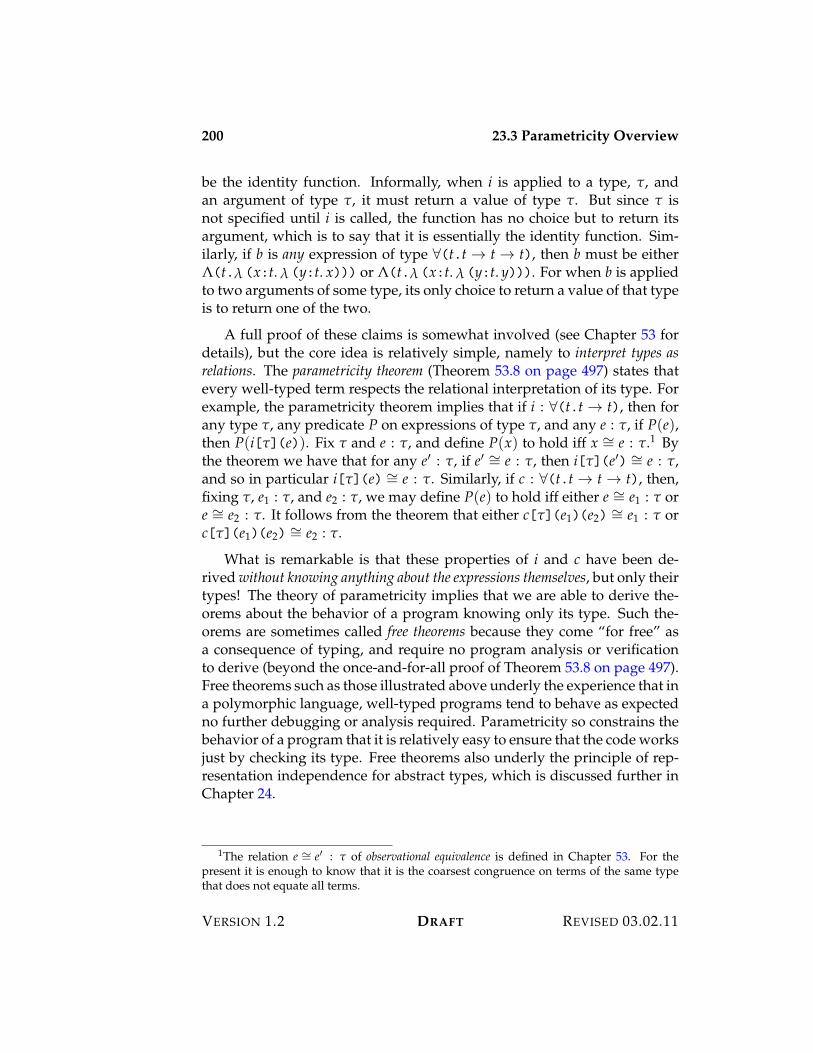
200 23.3 Parametricity Overview
be the identity function. Informally, when i is applied to a type, ", andan argument of type ", it must return a value of type ". But since " isnot specified until i is called, the function has no choice but to return itsargument, which is to say that it is essentially the identity function. Sim-ilarly, if b is any expression of type &(t.t 3 t 3 t), then b must be either((t.! (x:t. ! (y:t. x))) or ((t.! (x:t. ! (y:t. y))). For when b is appliedto two arguments of some type, its only choice to return a value of that typeis to return one of the two.
A full proof of these claims is somewhat involved (see Chapter 53 fordetails), but the core idea is relatively simple, namely to interpret types asrelations. The parametricity theorem (Theorem 53.8 on page 497) states thatevery well-typed term respects the relational interpretation of its type. Forexample, the parametricity theorem implies that if i : &(t.t 3 t), then forany type ", any predicate P on expressions of type ", and any e : ", if P(e),then P(i["](e)). Fix " and e : ", and define P(x) to hold iff x I= e : ".1 Bythe theorem we have that for any e% : ", if e% I= e : ", then i["](e%) I= e : ",and so in particular i["](e) I= e : ". Similarly, if c : &(t.t 3 t 3 t), then,fixing ", e1 : ", and e2 : ", we may define P(e) to hold iff either e I= e1 : " ore I= e2 : ". It follows from the theorem that either c["](e1)(e2) I= e1 : " orc["](e1)(e2) I= e2 : ".
What is remarkable is that these properties of i and c have been de-rived without knowing anything about the expressions themselves, but only theirtypes! The theory of parametricity implies that we are able to derive the-orems about the behavior of a program knowing only its type. Such the-orems are sometimes called free theorems because they come “for free” asa consequence of typing, and require no program analysis or verificationto derive (beyond the once-and-for-all proof of Theorem 53.8 on page 497).Free theorems such as those illustrated above underly the experience that ina polymorphic language, well-typed programs tend to behave as expectedno further debugging or analysis required. Parametricity so constrains thebehavior of a program that it is relatively easy to ensure that the code worksjust by checking its type. Free theorems also underly the principle of rep-resentation independence for abstract types, which is discussed further inChapter 24.
1The relation e I= e% : " of observational equivalence is defined in Chapter 53. For thepresent it is enough to know that it is the coarsest congruence on terms of the same typethat does not equate all terms.
VERSION 1.2 DRAFT REVISED 03.02.11
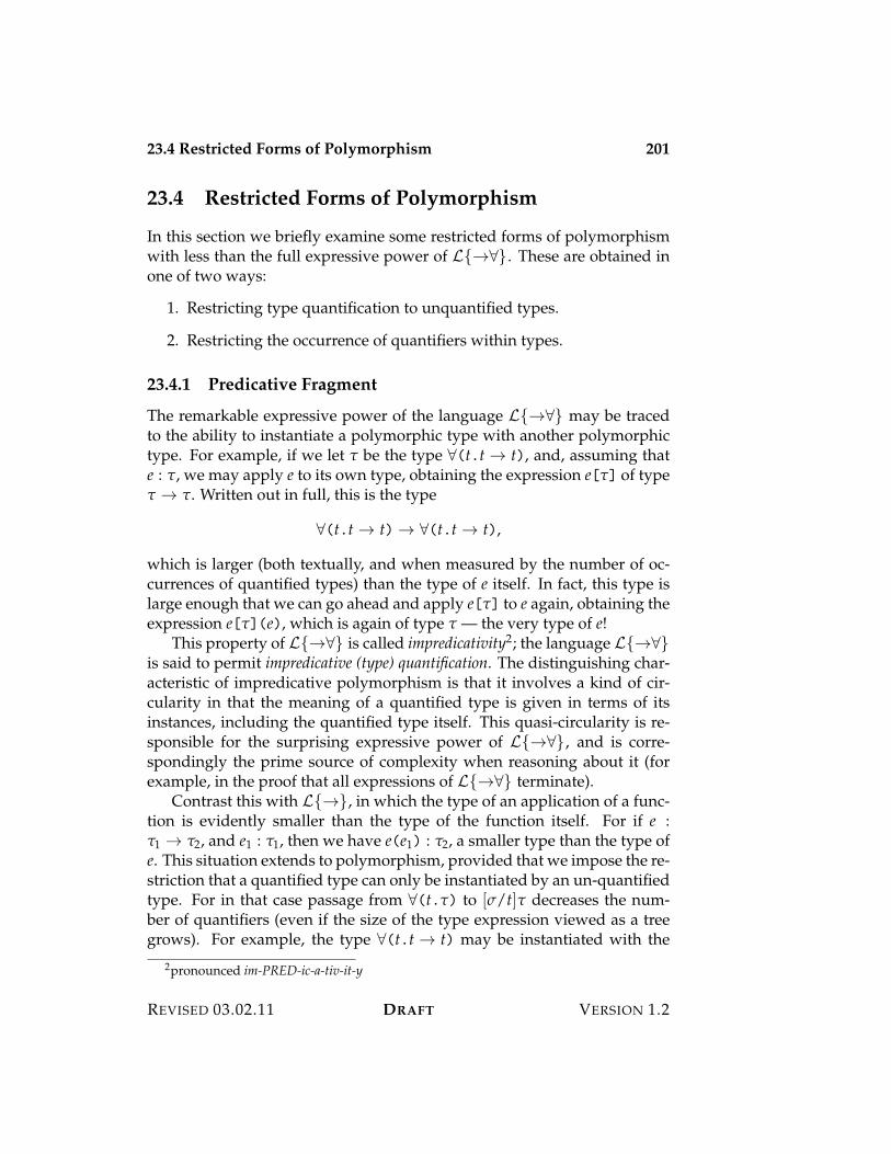
23.4 Restricted Forms of Polymorphism 201
23.4 Restricted Forms of Polymorphism
In this section we briefly examine some restricted forms of polymorphismwith less than the full expressive power of L{3&}. These are obtained inone of two ways:
1. Restricting type quantification to unquantified types.
2. Restricting the occurrence of quantifiers within types.
23.4.1 Predicative Fragment
The remarkable expressive power of the language L{3&} may be tracedto the ability to instantiate a polymorphic type with another polymorphictype. For example, if we let " be the type &(t.t 3 t), and, assuming thate : ", we may apply e to its own type, obtaining the expression e["] of type" 3 ". Written out in full, this is the type
&(t.t 3 t) 3 &(t.t 3 t),
which is larger (both textually, and when measured by the number of oc-currences of quantified types) than the type of e itself. In fact, this type islarge enough that we can go ahead and apply e["] to e again, obtaining theexpression e["](e), which is again of type " — the very type of e!
This property of L{3&} is called impredicativity2; the language L{3&}is said to permit impredicative (type) quantification. The distinguishing char-acteristic of impredicative polymorphism is that it involves a kind of cir-cularity in that the meaning of a quantified type is given in terms of itsinstances, including the quantified type itself. This quasi-circularity is re-sponsible for the surprising expressive power of L{3&}, and is corre-spondingly the prime source of complexity when reasoning about it (forexample, in the proof that all expressions of L{3&} terminate).
Contrast this with L{3}, in which the type of an application of a func-tion is evidently smaller than the type of the function itself. For if e :"1 3 "2, and e1 : "1, then we have e(e1) : "2, a smaller type than the type ofe. This situation extends to polymorphism, provided that we impose the re-striction that a quantified type can only be instantiated by an un-quantifiedtype. For in that case passage from &(t.") to [&/t]" decreases the num-ber of quantifiers (even if the size of the type expression viewed as a treegrows). For example, the type &(t.t 3 t) may be instantiated with the
2pronounced im-PRED-ic-a-tiv-it-y
REVISED 03.02.11 DRAFT VERSION 1.2
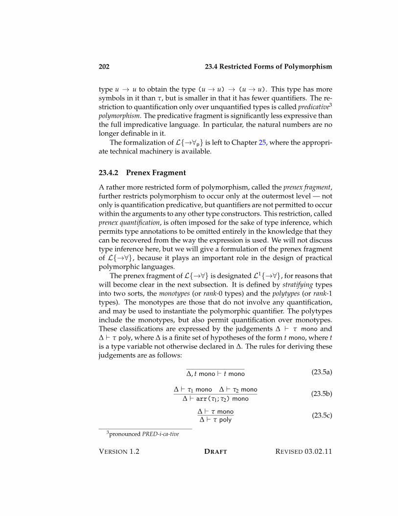
202 23.4 Restricted Forms of Polymorphism
type u 3 u to obtain the type (u 3 u) 3 (u 3 u). This type has moresymbols in it than ", but is smaller in that it has fewer quantifiers. The re-striction to quantification only over unquantified types is called predicative3
polymorphism. The predicative fragment is significantly less expressive thanthe full impredicative language. In particular, the natural numbers are nolonger definable in it.
The formalization of L{3&p} is left to Chapter 25, where the appropri-ate technical machinery is available.
23.4.2 Prenex Fragment
A rather more restricted form of polymorphism, called the prenex fragment,further restricts polymorphism to occur only at the outermost level — notonly is quantification predicative, but quantifiers are not permitted to occurwithin the arguments to any other type constructors. This restriction, calledprenex quantification, is often imposed for the sake of type inference, whichpermits type annotations to be omitted entirely in the knowledge that theycan be recovered from the way the expression is used. We will not discusstype inference here, but we will give a formulation of the prenex fragmentof L{3&}, because it plays an important role in the design of practicalpolymorphic languages.
The prenex fragment of L{3&} is designated L1{3&}, for reasons thatwill become clear in the next subsection. It is defined by stratifying typesinto two sorts, the monotypes (or rank-0 types) and the polytypes (or rank-1types). The monotypes are those that do not involve any quantification,and may be used to instantiate the polymorphic quantifier. The polytypesinclude the monotypes, but also permit quantification over monotypes.These classifications are expressed by the judgements " ) " mono and" ) " poly, where " is a finite set of hypotheses of the form t mono, where tis a type variable not otherwise declared in ". The rules for deriving thesejudgements are as follows:
", t mono ) t mono (23.5a)
" ) "1 mono " ) "2 mono" ) arr("1; "2) mono
(23.5b)
" ) " mono" ) " poly
(23.5c)
3pronounced PRED-i-ca-tive
VERSION 1.2 DRAFT REVISED 03.02.11
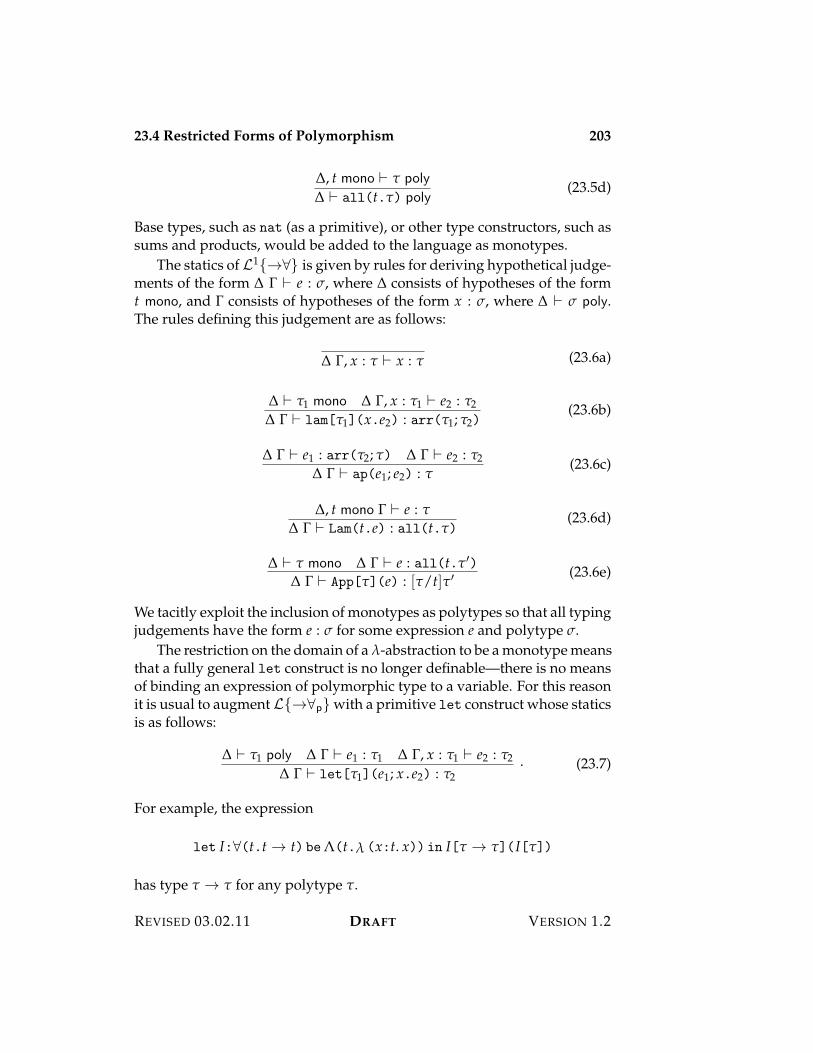
23.4 Restricted Forms of Polymorphism 203
", t mono ) " poly" ) all(t.") poly
(23.5d)
Base types, such as nat (as a primitive), or other type constructors, such assums and products, would be added to the language as monotypes.
The statics of L1{3&} is given by rules for deriving hypothetical judge-ments of the form " ! ) e : &, where " consists of hypotheses of the formt mono, and ! consists of hypotheses of the form x : &, where " ) & poly.The rules defining this judgement are as follows:
" !, x : " ) x : " (23.6a)
" ) "1 mono " !, x : "1 ) e2 : "2" ! ) lam["1](x.e2) : arr("1; "2)
(23.6b)
" ! ) e1 : arr("2; ") " ! ) e2 : "2" ! ) ap(e1; e2) : "
(23.6c)
", t mono ! ) e : "" ! ) Lam(t.e) : all(t.")
(23.6d)
" ) " mono " ! ) e : all(t."%)" ! ) App["](e) : ["/t]"% (23.6e)
We tacitly exploit the inclusion of monotypes as polytypes so that all typingjudgements have the form e : & for some expression e and polytype &.
The restriction on the domain of a !-abstraction to be a monotype meansthat a fully general let construct is no longer definable—there is no meansof binding an expression of polymorphic type to a variable. For this reasonit is usual to augment L{3&p} with a primitive let construct whose staticsis as follows:
" ) "1 poly " ! ) e1 : "1 " !, x : "1 ) e2 : "2" ! ) let["1](e1; x.e2) : "2
. (23.7)
For example, the expression
let I:&(t.t 3 t) be((t.! (x:t. x)) in I[" 3 "](I["])
has type " 3 " for any polytype ".
REVISED 03.02.11 DRAFT VERSION 1.2
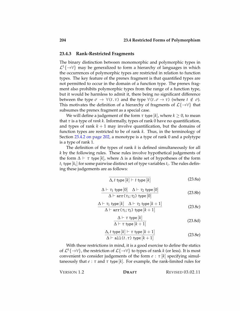
204 23.4 Restricted Forms of Polymorphism
23.4.3 Rank-Restricted Fragments
The binary distinction between monomorphic and polymorphic types inL1{3&} may be generalized to form a hierarchy of languages in whichthe occurrences of polymorphic types are restricted in relation to functiontypes. The key feature of the prenex fragment is that quantified types arenot permitted to occur in the domain of a function type. The prenex frag-ment also prohibits polymorphic types from the range of a function type,but it would be harmless to admit it, there being no significant differencebetween the type & 3 &(t.") and the type &(t.& 3 ") (where t /+ &).This motivates the definition of a hierarchy of fragments of L{3&} thatsubsumes the prenex fragment as a special case.
We will define a judgement of the form " type [k], where k 7 0, to meanthat " is a type of rank k. Informally, types of rank 0 have no quantification,and types of rank k + 1 may involve quantification, but the domains offunction types are restricted to be of rank k. Thus, in the terminology ofSection 23.4.2 on page 202, a monotype is a type of rank 0 and a polytypeis a type of rank 1.
The definition of the types of rank k is defined simultaneously for allk by the following rules. These rules involve hypothetical judgements ofthe form " ) " type [k], where " is a finite set of hypotheses of the formti type [ki] for some pairwise distinct set of type variables ti. The rules defin-ing these judgements are as follows:
", t type [k] ) t type [k] (23.8a)
" ) "1 type [0] " ) "2 type [0]" ) arr("1; "2) type [0]
(23.8b)
" ) "1 type [k] " ) "2 type [k + 1]" ) arr("1; "2) type [k + 1]
(23.8c)
" ) " type [k]" ) " type [k + 1]
(23.8d)
", t type [k] ) " type [k + 1]" ) all(t.") type [k + 1]
(23.8e)
With these restrictions in mind, it is a good exercise to define the staticsof Lk{3&}, the restriction of L{3&} to types of rank k (or less). It is mostconvenient to consider judgements of the form e : " [k] specifying simul-taneously that e : " and " type [k]. For example, the rank-limited rules for
VERSION 1.2 DRAFT REVISED 03.02.11

23.5 Exercises 205
!-abstractions is phrased as follows:
" ) "1 type [0] " !, x : "1 [0] ) e2 : "2 [0]" ! ) lam["1](x.e2) : arr("1; "2) [0]
(23.9a)
" ) "1 type [k] " !, x : "1 [k] ) e2 : "2 [k + 1]" ! ) lam["1](x.e2) : arr("1; "2) [k + 1]
(23.9b)
The remaining rules follow a similar pattern.The rank-limited languages Lk{3&} clarifies the requirement for a prim-
itive let construct in L1{3&}. The prenex fragment of L{3&} corre-sponds to the rank-one fragment L1{3&}. The let construct for rank-one types is definable in L2{3&} from !-abstraction and application. Thisdefinition only makes sense at rank two, since it abstracts over a rank-onepolymorphic type.
23.5 Exercises
1. Show that primitive recursion is definable in L{3&} by exploitingthe definability of iteration and binary products.
2. Investigate the representation of eager products and sums in eagerand lazy variants of L{3&}.
3. Show how to write an interpreter for L{nat3} in L{3&}.
REVISED 03.02.11 DRAFT VERSION 1.2

206 23.5 Exercises
VERSION 1.2 DRAFT REVISED 03.02.11
Chapter 24
Abstract Types
Data abstraction is perhaps the most important technique for structuringprograms. The main idea is to introduce an interface that serves as a contractbetween the client and the implementor of an abstract type. The interfacespecifies what the client may rely on for its own work, and, simultaneously,what the implementor must provide to satisfy the contract. The interfaceserves to isolate the client from the implementor so that each may be devel-oped in isolation from the other. In particular one implementation may bereplaced by another without affecting the behavior of the client, providedthat the two implementations meet the same interface and are, in a senseto be made precise below, suitably related to one another. (Roughly, eachsimulates the other with respect to the operations in the interface.) Thisproperty is called representation independence for an abstract type.
Data abstraction may be formalized by extending the language L{3&}with existential types. Interfaces are modelled as existential types that pro-vide a collection of operations acting on an unspecified, or abstract, type.Implementations are modelled as packages, the introductory form for exis-tentials, and clients are modelled as uses of the corresponding eliminationform. It is remarkable that the programming concept of data abstractionis modelled so naturally and directly by the logical concept of existentialtype quantification. Existential types are closely connected with universaltypes, and hence are often treated together. The superficial reason is thatboth are forms of type quantification, and hence both require the machin-ery of type variables. The deeper reason is that existentials are definablefrom universals — surprisingly, data abstraction is actually just a form ofpolymorphism! One consequence of this observation is that representationindependence is just a use of the parametricity properties of polymorphic
208 24.1 Existential Types
functions discussed in Chapter 23.
24.1 Existential Types
The syntax of L{3&'} is the extension of L{3&} with the following con-structs:
Type " ::= some(t.") '(t.") interfaceExpr e ::= pack[t."][,](e) pack , with e as '(t.") implementation
open[t."][,](e1; t, x.e2) open e1 as t with x:" in e2 client
The introductory form for the existential type & = '(t.") is a package ofthe form pack , with e as '(t."), where , is a type and e is an expression oftype [,/t]". The type , is called the representation type of the package, andthe expression e is called the implementation of the package. The elimina-tory form for existentials is the expression open e1 as t with x:" in e2, whichopens the package e1 for use within the client e2 by binding its representa-tion type to t and its implementation to x for use within e2. Crucially, thetyping rules ensure that the client is type-correct independently of the ac-tual representation type used by the implementor, so that it may be variedwithout affecting the type correctness of the client.
The abstract syntax of the open construct specifies that the type variable,t, and the expression variable, x, are bound within the client. They may berenamed at will by $-equivalence without affecting the meaning of the con-struct, provided, of course, that the names are chosen so as not to conflictwith any others that may be in scope. In other words the type, t, may bethought of as a “new” type, one that is distinct from all other types, whenit is introduced. This is sometimes called generativity of abstract types: theuse of an abstract type by a client “generates” a “new” type within thatclient. This behavior is simply a consequence of identifying terms up to$-equivalence, and is not particularly tied to data abstraction.
24.1.1 Statics
The statics of existential types is specified by rules defining when an exis-tential is well-formed, and by giving typing rules for the associated intro-ductory and eliminatory forms.
", t type ) " type" ) some(t.") type
(24.1a)
VERSION 1.2 DRAFT REVISED 03.02.11
24.1 Existential Types 209
" ) , type ", t type ) " type " ! ) e : [,/t]"" ! ) pack[t."][,](e) : some(t.")
(24.1b)
" ! ) e1 : some(t.") ", t type !, x : " ) e2 : "2 " ) "2 type" ! ) open[t."]["2](e1; t, x.e2) : "2
(24.1c)
Rule (24.1c) is complex, so study it carefully! There are two importantthings to notice:
1. The type of the client, "2, must not involve the abstract type t. Thisrestriction prevents the client from attempting to export a value of theabstract type outside of the scope of its definition.
2. The body of the client, e2, is type checked without knowledge of therepresentation type, t. The client is, in effect, polymorphic in the typevariable t.
Lemma 24.1 (Regularity). Suppose that " ! ) e : ". If " ) "i type for eachxi : "i in !, then " ) " type.
Proof. By induction on Rules (24.1).
24.1.2 Dynamics
The (eager or lazy) dynamics of existential types is specified as follows:
{e val}pack[t."][,](e) val
(24.2a)
&e 53 e%
pack[t."][,](e) 53 pack[t."][,](e%)
'(24.2b)
e1 53 e%1open[t."]["2](e1; t, x.e2) 53 open[t."]["2](e%1; t, x.e2)
(24.2c)
{e val}open[t."]["2](pack[t."][,](e); t, x.e2) 53 [,, e/t, x]e2
(24.2d)
It is important to observe that, according to these rules, there are no abstracttypes at run time! The representation type is propagated to the client by sub-stitution when the package is opened, thereby eliminating the abstractionboundary between the client and the implementor. Thus, data abstractionis a compile-time discipline that leaves no traces of its presence at executiontime.
REVISED 03.02.11 DRAFT VERSION 1.2
210 24.2 Data Abstraction Via Existentials
24.1.3 Safety
The safety of the extension is stated and proved as usual. The argument isa simple extension of that used for L{3&} to the new constructs.
Theorem 24.2 (Preservation). If e : " and e 53 e%, then e% : ".
Proof. By rule induction on e 53 e%, making use of substitution for bothexpression- and type variables.
Lemma 24.3 (Canonical Forms). If e : some(t.") and e val, then e = pack[t."][,](e%)for some type , and some e% such that e% : [,/t]".
Proof. By rule induction on the statics, making use of the definition of closedvalues.
Theorem 24.4 (Progress). If e : " then either e val or there exists e% such thate 53 e%.
Proof. By rule induction on e : ", making use of the canonical forms lemma.
24.2 Data Abstraction Via Existentials
To illustrate the use of existentials for data abstraction, we consider an ab-stract type of queues of natural numbers supporting three operations:
1. Formation of the empty queue.
2. Inserting an element at the tail of the queue.
3. Remove the head of the queue.
This is clearly a bare-bones interface, but is sufficient to illustrate the mainideas of data abstraction. Queue elements may be taken to be of any type,", of our choosing; we will not be specific about this choice, since nothingdepends on it.
The crucial property of this description is that nowhere do we specifywhat queues actually are, only what we can do with them. This is capturedby the following existential type, '(t."), which serves as the interface ofthe queue abstraction:
'(t.?emp : t, ins : nat< t 3 t, rem : t 3 nat< t@).
VERSION 1.2 DRAFT REVISED 03.02.11
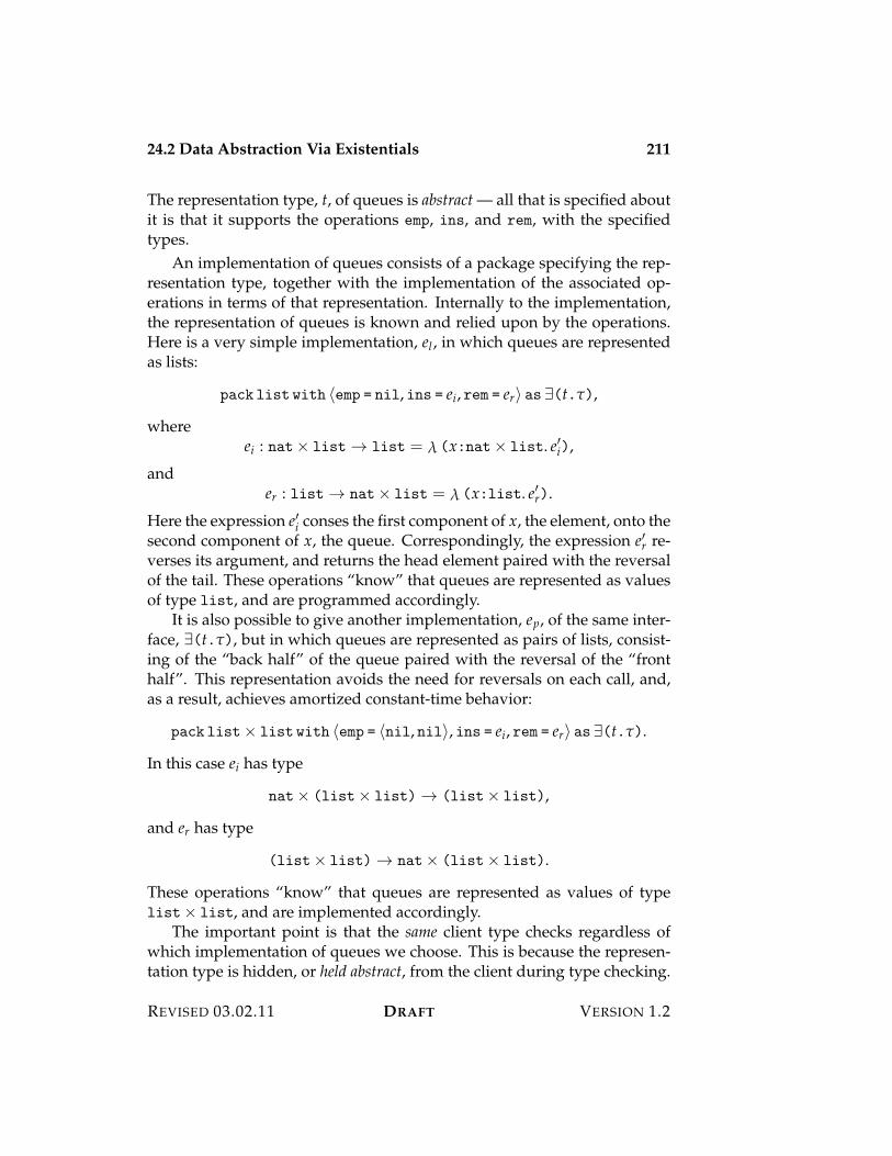
24.2 Data Abstraction Via Existentials 211
The representation type, t, of queues is abstract — all that is specified aboutit is that it supports the operations emp, ins, and rem, with the specifiedtypes.
An implementation of queues consists of a package specifying the rep-resentation type, together with the implementation of the associated op-erations in terms of that representation. Internally to the implementation,the representation of queues is known and relied upon by the operations.Here is a very simple implementation, el , in which queues are representedas lists:
pack list with ?emp = nil, ins = ei, rem = er@ as '(t."),
whereei : nat< list 3 list = ! (x:nat< list. e%i),
ander : list 3 nat< list = ! (x:list. e%r).
Here the expression e%i conses the first component of x, the element, onto thesecond component of x, the queue. Correspondingly, the expression e%r re-verses its argument, and returns the head element paired with the reversalof the tail. These operations “know” that queues are represented as valuesof type list, and are programmed accordingly.
It is also possible to give another implementation, ep, of the same inter-face, '(t."), but in which queues are represented as pairs of lists, consist-ing of the “back half” of the queue paired with the reversal of the “fronthalf”. This representation avoids the need for reversals on each call, and,as a result, achieves amortized constant-time behavior:
pack list< list with ?emp = ?nil, nil@, ins = ei, rem = er@ as '(t.").
In this case ei has type
nat< (list< list) 3 (list< list),
and er has type
(list< list) 3 nat< (list< list).
These operations “know” that queues are represented as values of typelist< list, and are implemented accordingly.
The important point is that the same client type checks regardless ofwhich implementation of queues we choose. This is because the represen-tation type is hidden, or held abstract, from the client during type checking.
REVISED 03.02.11 DRAFT VERSION 1.2
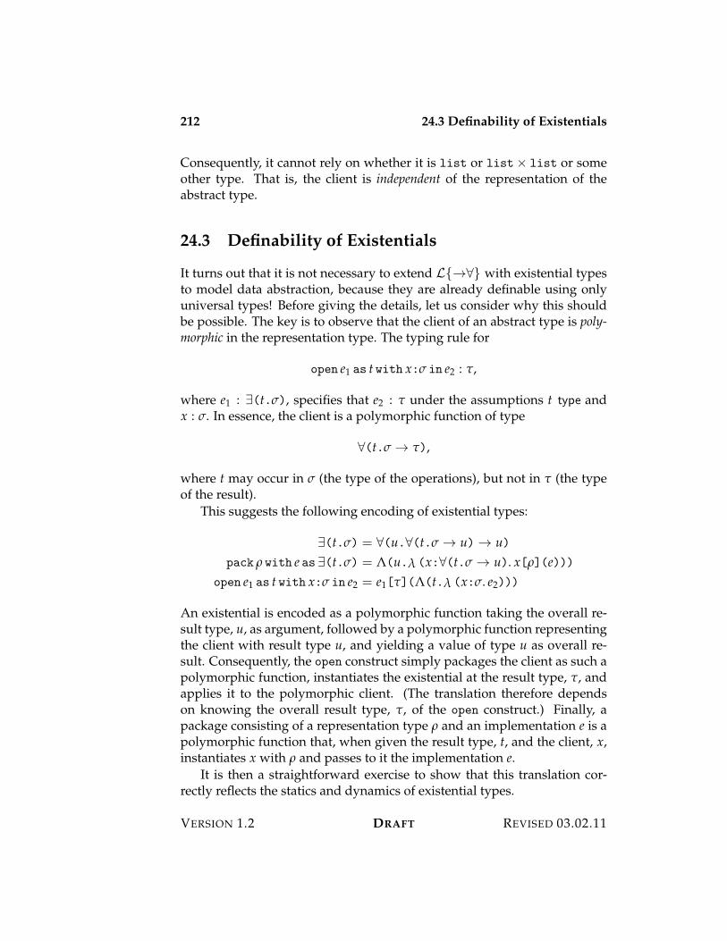
212 24.3 Definability of Existentials
Consequently, it cannot rely on whether it is list or list< list or someother type. That is, the client is independent of the representation of theabstract type.
24.3 Definability of Existentials
It turns out that it is not necessary to extend L{3&} with existential typesto model data abstraction, because they are already definable using onlyuniversal types! Before giving the details, let us consider why this shouldbe possible. The key is to observe that the client of an abstract type is poly-morphic in the representation type. The typing rule for
open e1 as t with x:& in e2 : ",
where e1 : '(t.&), specifies that e2 : " under the assumptions t type andx : &. In essence, the client is a polymorphic function of type
&(t.& 3 "),
where t may occur in & (the type of the operations), but not in " (the typeof the result).
This suggests the following encoding of existential types:
'(t.&) = &(u.&(t.& 3 u) 3 u)pack , with e as '(t.&) = ((u.! (x:&(t.& 3 u). x[,](e)))
open e1 as t with x:& in e2 = e1["](((t.! (x:&. e2)))
An existential is encoded as a polymorphic function taking the overall re-sult type, u, as argument, followed by a polymorphic function representingthe client with result type u, and yielding a value of type u as overall re-sult. Consequently, the open construct simply packages the client as such apolymorphic function, instantiates the existential at the result type, ", andapplies it to the polymorphic client. (The translation therefore dependson knowing the overall result type, ", of the open construct.) Finally, apackage consisting of a representation type , and an implementation e is apolymorphic function that, when given the result type, t, and the client, x,instantiates x with , and passes to it the implementation e.
It is then a straightforward exercise to show that this translation cor-rectly reflects the statics and dynamics of existential types.
VERSION 1.2 DRAFT REVISED 03.02.11
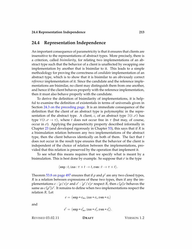
24.4 Representation Independence 213
24.4 Representation Independence
An important consequence of parametricity is that it ensures that clients areinsensitive to the representations of abstract types. More precisely, there isa criterion, called bisimilarity, for relating two implementations of an ab-stract type such that the behavior of a client is unaffected by swapping oneimplementation by another that is bisimilar to it. This leads to a simplemethodology for proving the correctness of candidate implementation of anabstract type, which is to show that it is bisimilar to an obviously correctreference implementation of it. Since the candidate and the reference imple-mentations are bisimilar, no client may distinguish them from one another,and hence if the client behaves properly with the reference implementation,then it must also behave properly with the candidate.
To derive the definition of bisimilarity of implementations, it is help-ful to examine the definition of existentials in terms of universals given inSection 24.3 on the preceding page. It is an immediate consequence of thedefinition that the client of an abstract type is polymorphic in the repre-sentation of the abstract type. A client, c, of an abstract type '(t.&) hastype &(t.& 3 "), where t does not occur free in " (but may, of course,occur in &). Applying the parametricity property described informally inChapter 23 (and developed rigorously in Chapter 53), this says that if R isa bisimulation relation between any two implementations of the abstracttype, then the client behaves identically on both of them. The fact that tdoes not occur in the result type ensures that the behavior of the client isindependent of the choice of relation between the implementations, pro-vided that this relation is preserved by the operation that implement it.
To see what this means requires that we specify what is meant by abisimulation. This is best done by example. So suppose that & is the type
?emp : t, ins : " < t 3 t, rem : t 3 " < t@.
Theorem 53.8 on page 497 ensures that if , and ,% are any two closed types,R is a relation between expressions of these two types, then if any the im-plementations e : [,/x]& and e% : [,%/x]& respect R, then c[,]e behaves thesame as c[,%]e%. It remains to define when two implementations respect therelation R. Let
e = ?emp = em, ins = ei, rem = er@
ande% = ?emp = e%m, ins = e%i , rem = e%r@.
REVISED 03.02.11 DRAFT VERSION 1.2
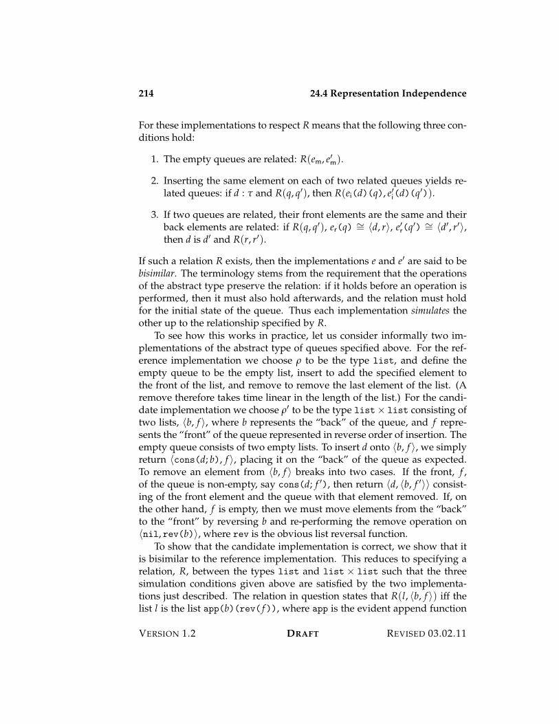
214 24.4 Representation Independence
For these implementations to respect R means that the following three con-ditions hold:
1. The empty queues are related: R(em, e%m).
2. Inserting the same element on each of two related queues yields re-lated queues: if d : " and R(q, q%), then R(ei(d)(q), e%i(d)(q%)).
3. If two queues are related, their front elements are the same and theirback elements are related: if R(q, q%), er(q) I= ?d, r@, e%r(q%) I= ?d%, r%@,then d is d% and R(r, r%).
If such a relation R exists, then the implementations e and e% are said to bebisimilar. The terminology stems from the requirement that the operationsof the abstract type preserve the relation: if it holds before an operation isperformed, then it must also hold afterwards, and the relation must holdfor the initial state of the queue. Thus each implementation simulates theother up to the relationship specified by R.
To see how this works in practice, let us consider informally two im-plementations of the abstract type of queues specified above. For the ref-erence implementation we choose , to be the type list, and define theempty queue to be the empty list, insert to add the specified element tothe front of the list, and remove to remove the last element of the list. (Aremove therefore takes time linear in the length of the list.) For the candi-date implementation we choose ,% to be the type list< list consisting oftwo lists, ?b, f @, where b represents the “back” of the queue, and f repre-sents the “front” of the queue represented in reverse order of insertion. Theempty queue consists of two empty lists. To insert d onto ?b, f @, we simplyreturn ?cons(d; b), f @, placing it on the “back” of the queue as expected.To remove an element from ?b, f @ breaks into two cases. If the front, f ,of the queue is non-empty, say cons(d; f %), then return ?d, ?b, f %@@ consist-ing of the front element and the queue with that element removed. If, onthe other hand, f is empty, then we must move elements from the “back”to the “front” by reversing b and re-performing the remove operation on?nil, rev(b)@, where rev is the obvious list reversal function.
To show that the candidate implementation is correct, we show that itis bisimilar to the reference implementation. This reduces to specifying arelation, R, between the types list and list < list such that the threesimulation conditions given above are satisfied by the two implementa-tions just described. The relation in question states that R(l, ?b, f @) iff thelist l is the list app(b)(rev( f)), where app is the evident append function
VERSION 1.2 DRAFT REVISED 03.02.11
24.5 Exercises 215
on lists. That is, thinking of l as the reference representation of the queue,the candidate must maintain that the elements of b followed by the ele-ments of f in reverse order form precisely the list l. It is easy to check thatthe implementations just described preserve this relation. Having done so,we are assured that the client, c, behaves the same regardless of whetherwe use the reference or the candidate. Since the reference implementationis obviously correct (albeit inefficient), the candidate must also be correctin that the behavior of any client is unaffected by using it instead of thereference.
24.5 Exercises
REVISED 03.02.11 DRAFT VERSION 1.2

216 24.5 Exercises
VERSION 1.2 DRAFT REVISED 03.02.11
Chapter 25
Constructors and Kinds
Types such as "1 3 "2 or " list may be thought of as being built from othertypes by the application of a type constructor, or type operator. These twoexamples differ from each other in that the function space type constructortakes two arguments, whereas the list type constructor takes only one. Wemay, for the sake of uniformity, think of types such as nat as being built bya type constructor of no arguments. More subtly, we may even think of thetypes &(t.") and '(t.") as being built up in the same way by regardingthe quantifiers as higher-order type operator.
These seemingly disparate cases may be treated uniformly by enrich-ing the syntactic structure of a language with a new layer of constructors.To ensure that constructors are used properly (for example, that the listconstructor is given only one argument, and that the function constructoris given two), we classify constructors by kinds. Constructors of a distin-guished kind, Type, are types, which may be used to classify expressions.To allow for multi-argument and higher-order constructors, we will alsoconsider finite product and function kinds. (Later we shall consider evenricher kinds.)
The distinction between constructors and kinds on one hand and typesand expressions on the other reflects a fundamental separation betweenthe static and dynamic phase of processing of a programming language,called the phase distinction. The static phase implements the statics and thedynamic phase implements the dynamics. Constructors may be seen as aform of static data that is manipulated during the static phase of process-ing. Expressions are a form of dynamic data that is manipulated at run-time.Since the dynamic phase follows the static phase (we only execute well-typed programs), we may also manipulate constructors at run-time.
218 25.1 Statics
Adding constructors and kinds to a language introduces more techni-cal complications than might at first be apparent. The main difficulty is thatas soon as we enrich the kind structure beyond the distinguished kind oftypes, it becomes essential to simplify constructors to determine whetherthey are equivalent. For example, if we admit product kinds, then a pair ofconstructors is a constructor of product kind, and projections from a con-structor of product kind are also constructors. But what if we form the firstprojection from the pair consisiting of the constructors nat and str? Thisshould be equivalent to nat, since the elimination form if post-inverse tothe introduction form. Consequently, any expression (say, a variable) of theone type should also be an expression of the other. That is, typing shouldrespect definitional equivalence of constructors.
There are two main ways to deal with this. One is to introduce a conceptof definitional equivalence for constructors, and to demand that the typingjudgement for expressions respect definitional equivalence of constructorsof kind Type. This means, however, that we must show that definitionalequivalence is decidable if we are to build a complete implementation ofthe language. The other is to prohibit formation of awkward constructorssuch as the projection from a pair so that there is never any issue of whentwo constructors are equivalent (only when they are identical). But thiscomplicates the definition of substitution, since a projection from a con-structor variable is well-formed, until you substitute a pair for the vari-able. Both approaches have their benefits, but the second is simplest, andis adopted here.
25.1 Statics
The syntax of kinds is given by the following grammar:
Kind . ::= Type Type typesUnit 1 nullary productProd(.1; .2) .1 < .2 binary productArr(.1; .2) .1 3 .2 function
The kinds consist of the kind of types, Type, the unit kind, Unit, and areclosed under formation of product and function kinds.
The syntax of constructors is divided into two syntactic sorts, the neutral
VERSION 1.2 DRAFT REVISED 03.02.11
25.1 Statics 219
and the canonical, according to the following grammar:
Neut a ::= u u variableproj[l](a) prl(a) first projectionproj[r](a) prr(a) second projectionapp(a1; c2) a1[c2] application
Canon c ::= atom(a) )a atomicunit ?@ null tuplepair(c1; c2) ?c1, c2@ pairlam(u.c) ! u.c abstraction
The reason to distinguish neutral from canonical constructors is to en-sure that it is impossible to apply an elimination form to an introductionform, which demands an equation to capture the inversion principle. Forexample, the putative constructor prl(?c1, c2@), which would be definition-ally equivalent to c1, is ill-formed according to Grammar (25.1). This isbecause the argument to a projection must be neutral, but a pair is onlycanonical, not neutral.
The canonical constructor atom(a) is the inclusion of neutral construc-tors into canonical constructors. However, the grammar does not capturea crucial property of the statics that ensures that only neutral constructorsof kind Type may be treated as canonical. This requirement is imposedto limit the forms of canonical contructors of the other kinds. In particular,variables of function, product, or unit kind will turn out not to be canonical,but only neutral.
The statics of constructors and kinds is specified by the judgements
" ) a : . neutral constructor formation" ) c " . canonical constructor formation
In each of these judgements " is a finite set of hypotheses of the form
u1 : .1, . . . , un : .n
for some n 7 0. The form of the hypotheses expresses the principle thatvariables are neutral constructors. The formation judgements are to beunderstood as generic hypothetical judgements with parameters u1, . . . , unthat are determined by the forms of the hypotheses.
The rules for constructor formation are as follows:
", u : . ) u : . (25.1a)
REVISED 03.02.11 DRAFT VERSION 1.2
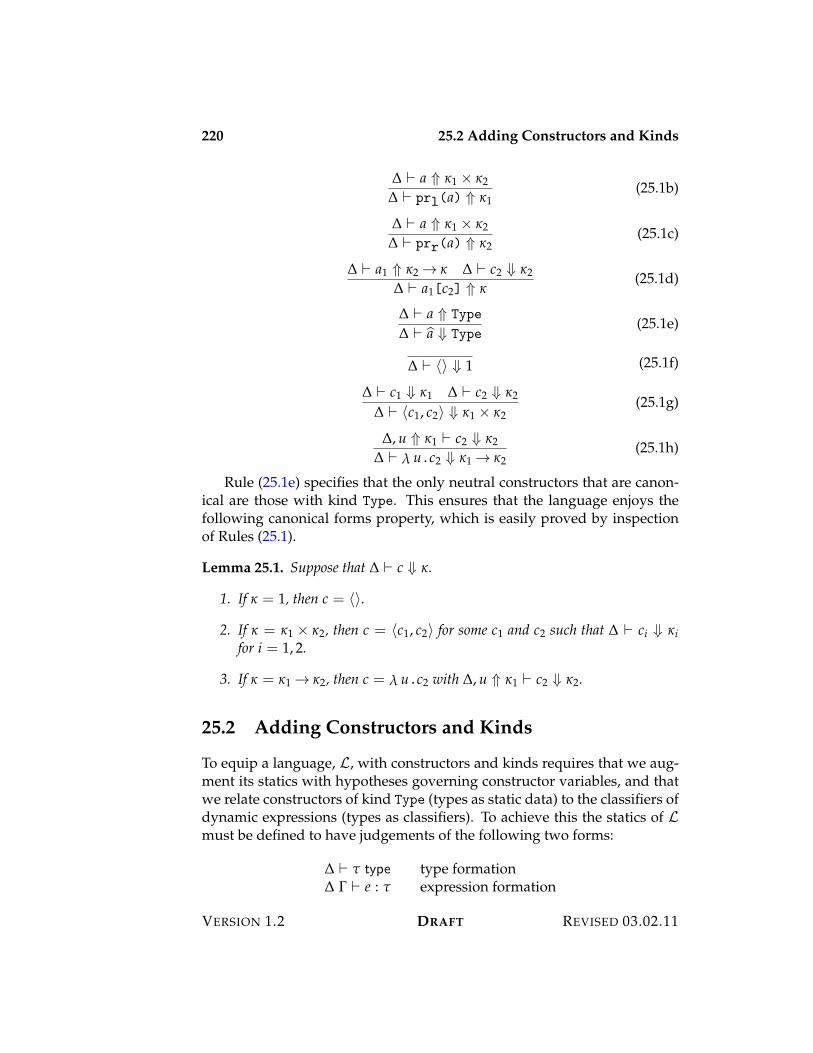
220 25.2 Adding Constructors and Kinds
" ) a : .1 < .2" ) prl(a) : .1
(25.1b)
" ) a : .1 < .2" ) prr(a) : .2
(25.1c)
" ) a1 : .2 3 . " ) c2 " .2" ) a1[c2] : .
(25.1d)
" ) a : Type
" ) )a " Type(25.1e)
" ) ?@ " 1 (25.1f)
" ) c1 " .1 " ) c2 " .2
" ) ?c1, c2@ " .1 < .2(25.1g)
", u : .1 ) c2 " .2" ) ! u.c2 " .1 3 .2
(25.1h)
Rule (25.1e) specifies that the only neutral constructors that are canon-ical are those with kind Type. This ensures that the language enjoys thefollowing canonical forms property, which is easily proved by inspectionof Rules (25.1).
Lemma 25.1. Suppose that " ) c " ..
1. If . = 1, then c = ?@.
2. If . = .1 < .2, then c = ?c1, c2@ for some c1 and c2 such that " ) ci " .ifor i = 1, 2.
3. If . = .1 3 .2, then c = ! u.c2 with ", u : .1 ) c2 " .2.
25.2 Adding Constructors and Kinds
To equip a language, L, with constructors and kinds requires that we aug-ment its statics with hypotheses governing constructor variables, and thatwe relate constructors of kind Type (types as static data) to the classifiers ofdynamic expressions (types as classifiers). To achieve this the statics of Lmust be defined to have judgements of the following two forms:
" ) " type type formation" ! ) e : " expression formation
VERSION 1.2 DRAFT REVISED 03.02.11
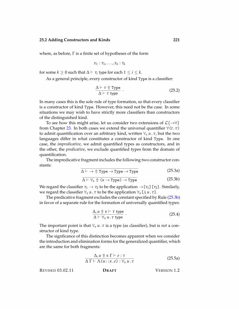
25.2 Adding Constructors and Kinds 221
where, as before, ! is a finite set of hypotheses of the form
x1 : "1, . . . , xk : "k
for some k 7 0 such that " ) "i type for each 1 ( i ( k.As a general principle, every constructor of kind Type is a classifier:
" ) " : Type
" ) " type. (25.2)
In many cases this is the sole rule of type formation, so that every classifieris a constructor of kind Type. However, this need not be the case. In somesituations we may wish to have strictly more classifiers than constructorsof the distinguished kind.
To see how this might arise, let us consider two extensions of L{3&}from Chapter 23. In both cases we extend the universal quantifier &(t.")to admit quantification over an arbitrary kind, written &. u.", but the twolanguages differ in what constitutes a constructor of kind Type. In onecase, the impredicative, we admit quantified types as constructors, and inthe other, the predicative, we exclude quantified types from the domain ofquantification.
The impredicative fragment includes the following two constructor con-stants:
" ) 3 : Type3 Type3 Type (25.3a)
" ) &. : (. 3 Type)3 Type (25.3b)
We regard the classifier "1 3 "2 to be the application 3["1]["2]. Similarly,we regard the classifier &. u." to be the application &.[! u."].
The predicative fragment excludes the constant specified by Rule (25.3b)in favor of a separate rule for the formation of universally quantified types:
", u : . ) " type" ) &. u." type
. (25.4)
The important point is that &. u." is a type (as classifier), but is not a con-structor of kind type.
The signficance of this distinction becomes apparent when we considerthe introduction and elimination forms for the generalized quantifier, whichare the same for both fragments:
", u : . ! ) e : "" ! ) ((u::..e) : &. u."
(25.5a)
REVISED 03.02.11 DRAFT VERSION 1.2
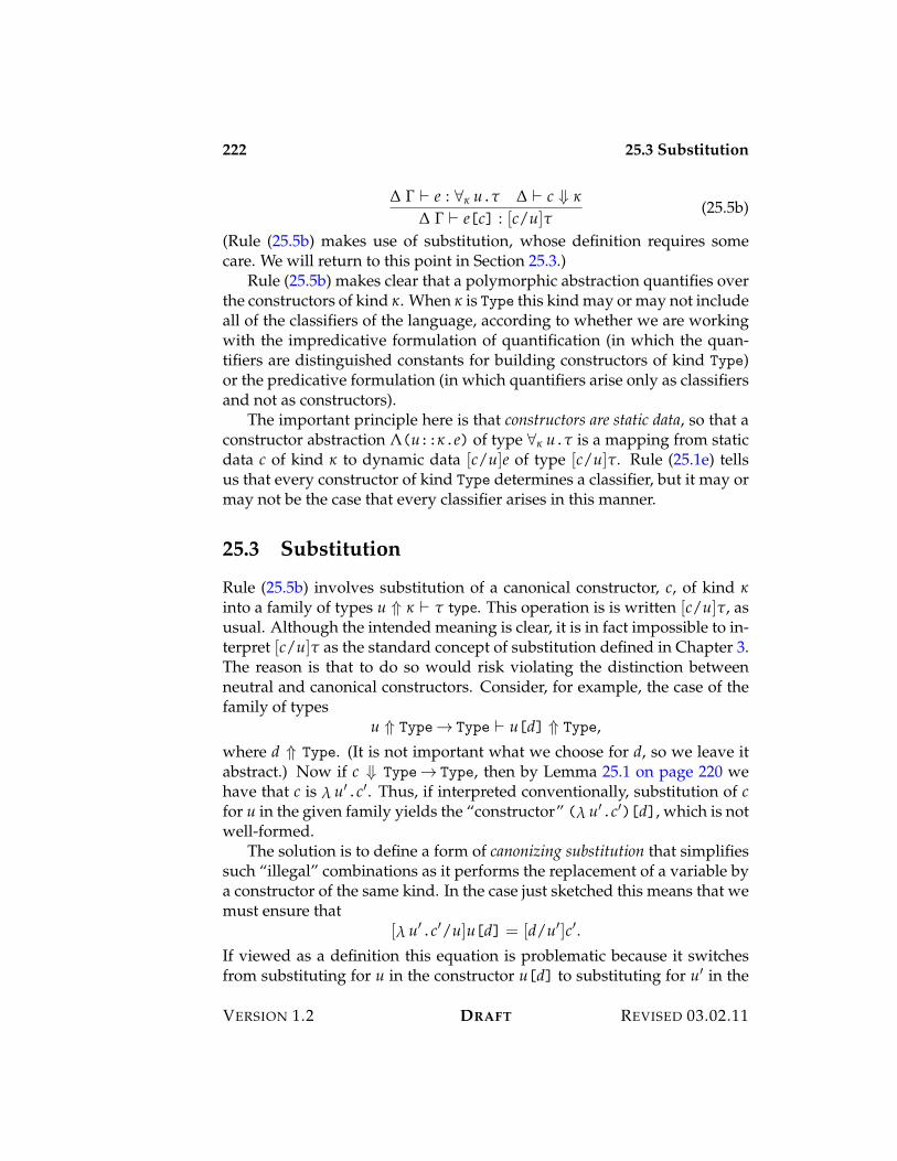
222 25.3 Substitution
" ! ) e : &. u." " ) c " .
" ! ) e[c] : [c/u]"(25.5b)
(Rule (25.5b) makes use of substitution, whose definition requires somecare. We will return to this point in Section 25.3.)
Rule (25.5b) makes clear that a polymorphic abstraction quantifies overthe constructors of kind .. When . is Type this kind may or may not includeall of the classifiers of the language, according to whether we are workingwith the impredicative formulation of quantification (in which the quan-tifiers are distinguished constants for building constructors of kind Type)or the predicative formulation (in which quantifiers arise only as classifiersand not as constructors).
The important principle here is that constructors are static data, so that aconstructor abstraction ((u::..e) of type &. u." is a mapping from staticdata c of kind . to dynamic data [c/u]e of type [c/u]". Rule (25.1e) tellsus that every constructor of kind Type determines a classifier, but it may ormay not be the case that every classifier arises in this manner.
25.3 Substitution
Rule (25.5b) involves substitution of a canonical constructor, c, of kind .into a family of types u : . ) " type. This operation is is written [c/u]", asusual. Although the intended meaning is clear, it is in fact impossible to in-terpret [c/u]" as the standard concept of substitution defined in Chapter 3.The reason is that to do so would risk violating the distinction betweenneutral and canonical constructors. Consider, for example, the case of thefamily of types
u : Type3 Type ) u[d] : Type,where d : Type. (It is not important what we choose for d, so we leave itabstract.) Now if c " Type3 Type, then by Lemma 25.1 on page 220 wehave that c is ! u%.c%. Thus, if interpreted conventionally, substitution of cfor u in the given family yields the “constructor” (! u%.c%)[d], which is notwell-formed.
The solution is to define a form of canonizing substitution that simplifiessuch “illegal” combinations as it performs the replacement of a variable bya constructor of the same kind. In the case just sketched this means that wemust ensure that
[! u%.c%/u]u[d] = [d/u%]c%.If viewed as a definition this equation is problematic because it switchesfrom substituting for u in the constructor u[d] to substituting for u% in the
VERSION 1.2 DRAFT REVISED 03.02.11
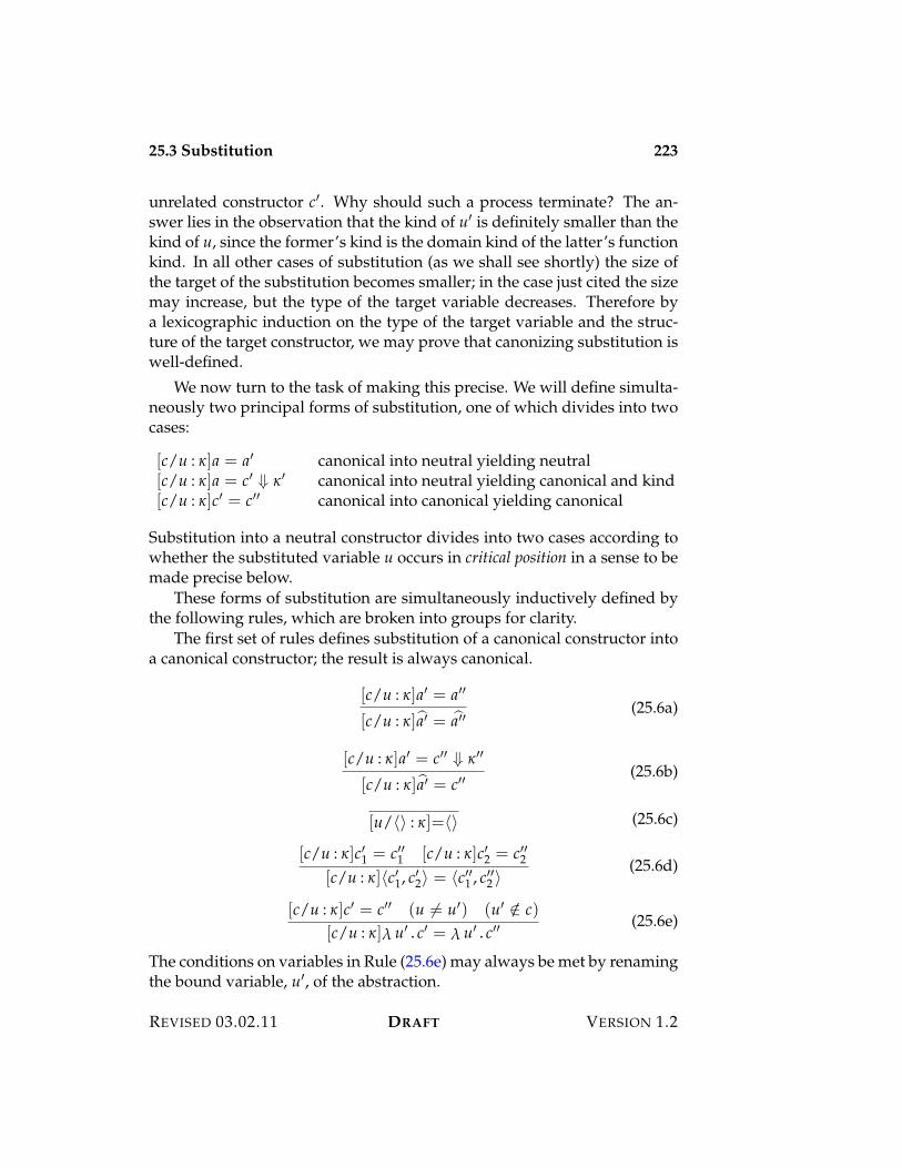
25.3 Substitution 223
unrelated constructor c%. Why should such a process terminate? The an-swer lies in the observation that the kind of u% is definitely smaller than thekind of u, since the former’s kind is the domain kind of the latter’s functionkind. In all other cases of substitution (as we shall see shortly) the size ofthe target of the substitution becomes smaller; in the case just cited the sizemay increase, but the type of the target variable decreases. Therefore bya lexicographic induction on the type of the target variable and the struc-ture of the target constructor, we may prove that canonizing substitution iswell-defined.
We now turn to the task of making this precise. We will define simulta-neously two principal forms of substitution, one of which divides into twocases:
[c/u : .]a = a% canonical into neutral yielding neutral[c/u : .]a = c% " .% canonical into neutral yielding canonical and kind[c/u : .]c% = c%% canonical into canonical yielding canonical
Substitution into a neutral constructor divides into two cases according towhether the substituted variable u occurs in critical position in a sense to bemade precise below.
These forms of substitution are simultaneously inductively defined bythe following rules, which are broken into groups for clarity.
The first set of rules defines substitution of a canonical constructor intoa canonical constructor; the result is always canonical.
[c/u : .]a% = a%%
[c/u : .])a% = )a%%(25.6a)
[c/u : .]a% = c%% " .%%
[c/u : .])a% = c%%(25.6b)
[u/?@ : .]=?@ (25.6c)
[c/u : .]c%1 = c%%1 [c/u : .]c%2 = c%%2[c/u : .]?c%1, c%2@ = ?c%%1 , c%%2 @
(25.6d)
[c/u : .]c% = c%% (u ,= u%) (u% /+ c)[c/u : .]! u%.c% = ! u%.c%%
(25.6e)
The conditions on variables in Rule (25.6e) may always be met by renamingthe bound variable, u%, of the abstraction.
REVISED 03.02.11 DRAFT VERSION 1.2
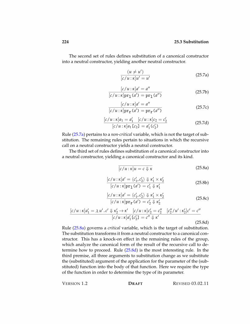
224 25.3 Substitution
The second set of rules defines substitution of a canonical constructorinto a neutral constructor, yielding another neutral constructor.
(u ,= u%)
[c/u : .]u% = u% (25.7a)
[c/u : .]a% = a%%
[c/u : .]prl(a%) = prl(a%%)(25.7b)
[c/u : .]a% = a%%
[c/u : .]prr(a%) = prr(a%%)(25.7c)
[c/u : .]a1 = a%1 [c/u : .]c2 = c%2[c/u : .]a1[c2] = a%1(c%2)
(25.7d)
Rule (25.7a) pertains to a non-critical variable, which is not the target of sub-stitution. The remaining rules pertain to situations in which the recursivecall on a neutral constructor yields a neutral constructor.
The third set of rules defines substitution of a canonical constructor intoa neutral constructor, yielding a canonical constructor and its kind.
[c/u : .]u = c " . (25.8a)
[c/u : .]a% = ?c%1, c%2@ " .%1 < .%2[c/u : .]prl(a%) = c%1 " .%1
(25.8b)
[c/u : .]a% = ?c%1, c%2@ " .%1 < .%2[c/u : .]prr(a%) = c%2 " .%2
(25.8c)
[c/u : .]a%1 = ! u%.c% " .%2 3 .% [c/u : .]c%2 = c%%2 [c%%2 /u% : .%2]c% = c%%
[c/u : .]a%1[c%2] = c%% " .%
(25.8d)Rule (25.8a) governs a critical variable, which is the target of substitution.The substitution transforms it from a neutral constructor to a canonical con-structor. This has a knock-on effect in the remaining rules of the group,which analyze the canonical form of the result of the recursive call to de-termine how to proceed. Rule (25.8d) is the most interesting rule. In thethird premise, all three arguments to substitution change as we substitutethe (substituted) argument of the application for the parameter of the (sub-stituted) function into the body of that function. Here we require the typeof the function in order to determine the type of its parameter.
VERSION 1.2 DRAFT REVISED 03.02.11
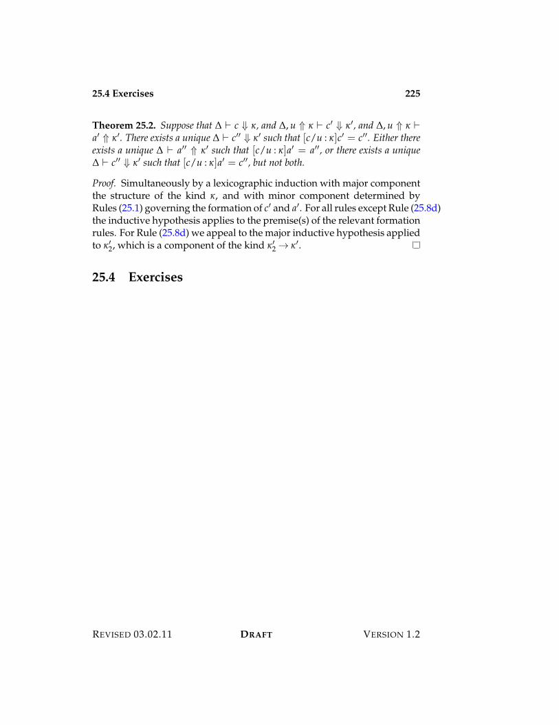
25.4 Exercises 225
Theorem 25.2. Suppose that " ) c " ., and ", u : . ) c% " .%, and ", u : . )a% : .%. There exists a unique " ) c%% " .% such that [c/u : .]c% = c%%. Either thereexists a unique " ) a%% : .% such that [c/u : .]a% = a%%, or there exists a unique" ) c%% " .% such that [c/u : .]a% = c%%, but not both.
Proof. Simultaneously by a lexicographic induction with major componentthe structure of the kind ., and with minor component determined byRules (25.1) governing the formation of c% and a%. For all rules except Rule (25.8d)the inductive hypothesis applies to the premise(s) of the relevant formationrules. For Rule (25.8d) we appeal to the major inductive hypothesis appliedto .%2, which is a component of the kind .%2 3 .%.
25.4 Exercises
REVISED 03.02.11 DRAFT VERSION 1.2

226 25.4 Exercises
VERSION 1.2 DRAFT REVISED 03.02.11
Chapter 26
Indexed Families of Types
26.1 Type Families
26.2 Exercises

228 26.2 Exercises
VERSION 1.2 DRAFT REVISED 03.02.11

Part IX
Subtyping

Chapter 27
Subtyping
A subtype relation is a pre-order (reflexive and transitive relation) on typesthat validates the subsumption principle:
if & is a subtype of ", then a value of type & may be providedwhenever a value of type " is required.
The subsumption principle relaxes the strictures of a type system to permitvalues of one type to be treated as values of another.
Experience shows that the subsumption principle, while useful as ageneral guide, can be tricky to apply correctly in practice. The key to get-ting it right is the principle of introduction and elimination. To determinewhether a candidate subtyping relationship is sensible, it suffices to con-sider whether every introductory form of the subtype can be safely manip-ulated by every eliminatory form of the supertype. A subtyping principlemakes sense only if it passes this test; the proof of the type safety theoremfor a given subtyping relation ensures that this is the case.
A good way to get a subtyping principle wrong is to think of a typemerely as a set of values (generated by introductory forms), and to considerwhether every value of the subtype can also be considered to be a value ofthe supertype. The intuition behind this approach is to think of subtypingas akin to the subset relation in ordinary mathematics. But this can lead toserious errors, because it fails to take account of the operations (eliminatoryforms) that one can perform on values of the supertype. It is not enough tothink only of the introductory forms; one must also think of the eliminatoryforms. Subtyping is a matter of behavior, rather than containment.
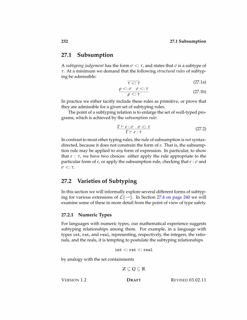
232 27.1 Subsumption
27.1 Subsumption
A subtyping judgement has the form & <: ", and states that & is a subtype of". At a minimum we demand that the following structural rules of subtyp-ing be admissible:
" <: " (27.1a), <: & & <: "
, <: " (27.1b)
In practice we either tacitly include these rules as primitive, or prove thatthey are admissible for a given set of subtyping rules.
The point of a subtyping relation is to enlarge the set of well-typed pro-grams, which is achieved by the subsumption rule:
! ) e : & & <: "! ) e : "
(27.2)
In contrast to most other typing rules, the rule of subsumption is not syntax-directed, because it does not constrain the form of e. That is, the subsump-tion rule may be applied to any form of expression. In particular, to showthat e : ", we have two choices: either apply the rule appropriate to theparticular form of e, or apply the subsumption rule, checking that e : & and& <: ".
27.2 Varieties of Subtyping
In this section we will informally explore several different forms of subtyp-ing for various extensions of L{"}. In Section 27.4 on page 240 we willexamine some of these in more detail from the point of view of type safety.
27.2.1 Numeric Types
For languages with numeric types, our mathematical experience suggestssubtyping relationships among them. For example, in a language withtypes int, rat, and real, representing, respectively, the integers, the ratio-nals, and the reals, it is tempting to postulate the subtyping relationships
int <: rat <: real
by analogy with the set containments
Z - Q - R
VERSION 1.2 DRAFT REVISED 03.02.11
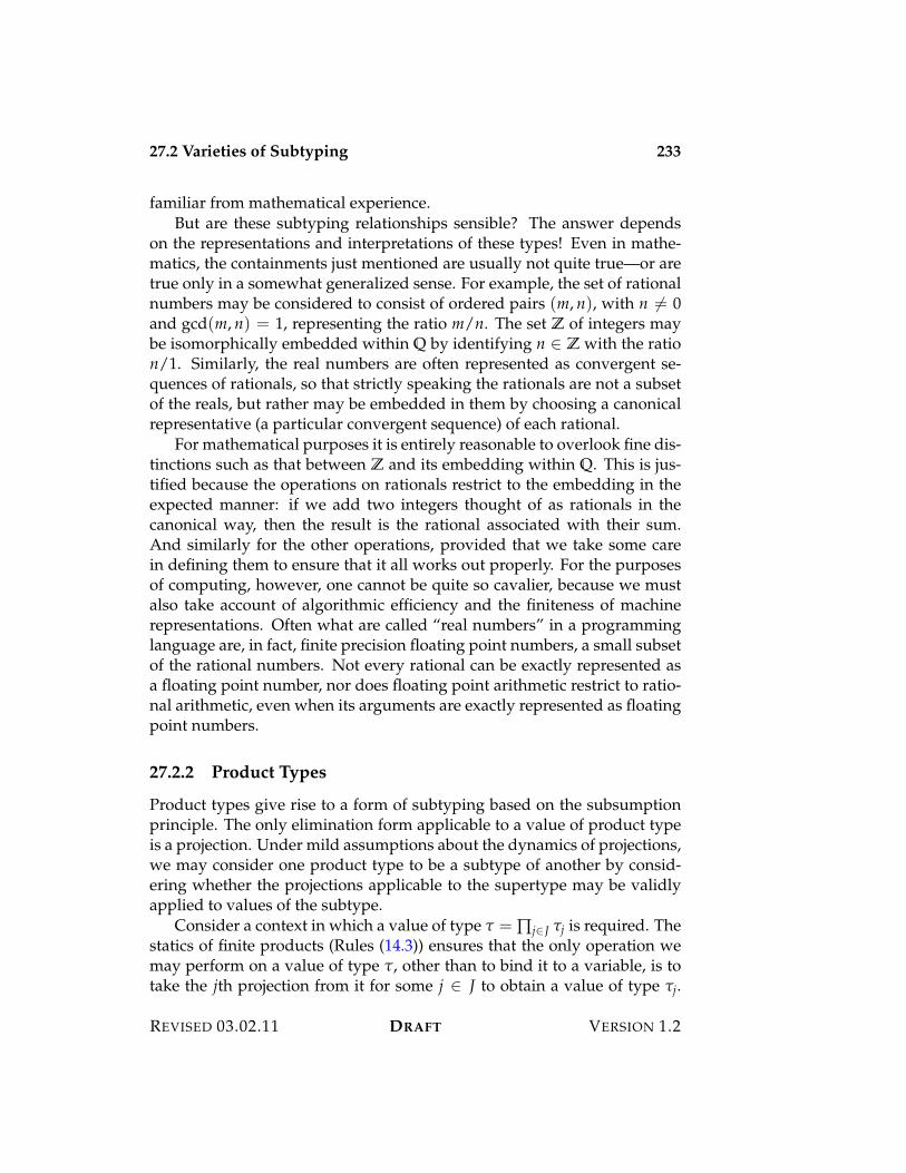
27.2 Varieties of Subtyping 233
familiar from mathematical experience.But are these subtyping relationships sensible? The answer depends
on the representations and interpretations of these types! Even in mathe-matics, the containments just mentioned are usually not quite true—or aretrue only in a somewhat generalized sense. For example, the set of rationalnumbers may be considered to consist of ordered pairs (m, n), with n ,= 0and gcd(m, n) = 1, representing the ratio m/n. The set Z of integers maybe isomorphically embedded within Q by identifying n + Z with the ration/1. Similarly, the real numbers are often represented as convergent se-quences of rationals, so that strictly speaking the rationals are not a subsetof the reals, but rather may be embedded in them by choosing a canonicalrepresentative (a particular convergent sequence) of each rational.
For mathematical purposes it is entirely reasonable to overlook fine dis-tinctions such as that between Z and its embedding within Q. This is jus-tified because the operations on rationals restrict to the embedding in theexpected manner: if we add two integers thought of as rationals in thecanonical way, then the result is the rational associated with their sum.And similarly for the other operations, provided that we take some carein defining them to ensure that it all works out properly. For the purposesof computing, however, one cannot be quite so cavalier, because we mustalso take account of algorithmic efficiency and the finiteness of machinerepresentations. Often what are called “real numbers” in a programminglanguage are, in fact, finite precision floating point numbers, a small subsetof the rational numbers. Not every rational can be exactly represented asa floating point number, nor does floating point arithmetic restrict to ratio-nal arithmetic, even when its arguments are exactly represented as floatingpoint numbers.
27.2.2 Product Types
Product types give rise to a form of subtyping based on the subsumptionprinciple. The only elimination form applicable to a value of product typeis a projection. Under mild assumptions about the dynamics of projections,we may consider one product type to be a subtype of another by consid-ering whether the projections applicable to the supertype may be validlyapplied to values of the subtype.
Consider a context in which a value of type " = &j+J "j is required. Thestatics of finite products (Rules (14.3)) ensures that the only operation wemay perform on a value of type ", other than to bind it to a variable, is totake the jth projection from it for some j + J to obtain a value of type "j.
REVISED 03.02.11 DRAFT VERSION 1.2

234 27.2 Varieties of Subtyping
Now suppose that e is of type &. If the projection e · j is to be well-formed,then & must be a finite product type &i+I &i such that j + I. Moreover, forthis to be of type "j, it is enough to require that &j = "j. Since j + J isarbitrary, we arrive at the following subtyping rule for finite product types:
J - I&i+I "i <: &j+J "j
. (27.3)
It is sufficient, but not necessary, to require that &j = "j for each j + J; wewill consider a more liberal form of this rule in Section 27.3 on page 236.
The argument for Rule (27.3) is based on a dynamics in which we mayevaluate e · j regardless of the actual form of e, provided only that it has afield indexed by j + J. Is this a reasonable assumption?
One common case is that I and J are initial segments of the naturalnumbers, say I = [0..m $ 1] and J = [0..n $ 1], so that the product typesmay be thought of as m- and n-tuples, respectively. The containment I -J amounts to requiring that m 7 n, which is to say that a tuple type isregarded as a subtype of all of its prefixes. When specialized to this case,Rule (27.3) may be stated in the form
m 7 n?"1, . . . , "m@ <: ?"1, . . . , "n@
. (27.4)
One way to justify this rule is to consider elements of the subtype to beconsecutive sequences of values of type "0, . . . , "m$1 from which we maycalculate the jth projection for any 0 ( j < n ( m, regardless of whether ornot m is strictly bigger than n.
Another common case is when I and J are finite sets of symbols, sothat projections are based on the field name, rather than its position. Whenspecialized to this case, Rule (27.3) takes the following form:
m 7 n?l1 : "1, . . . , lm : "m@ <: ?l1 : "1, . . . , ln : "n@
. (27.5)
Here we are taking advantage of the implicit identification of labeled tupletypes up to reordering of fields, so that the rule states that any field of thesupertype must be present in the subtype with the same type.
When using symbolic labels for the components of a tuple, it is perhapsslightly less clear that Rule (27.5) is well-justified. After all, how are we tofind field li, where 0 ( i < n, in a labeled tuple that may have additionalfields anywhere within it? The trouble is that the label does not reveal theposition of the field within the tuple, precisely because of subtyping. One
VERSION 1.2 DRAFT REVISED 03.02.11
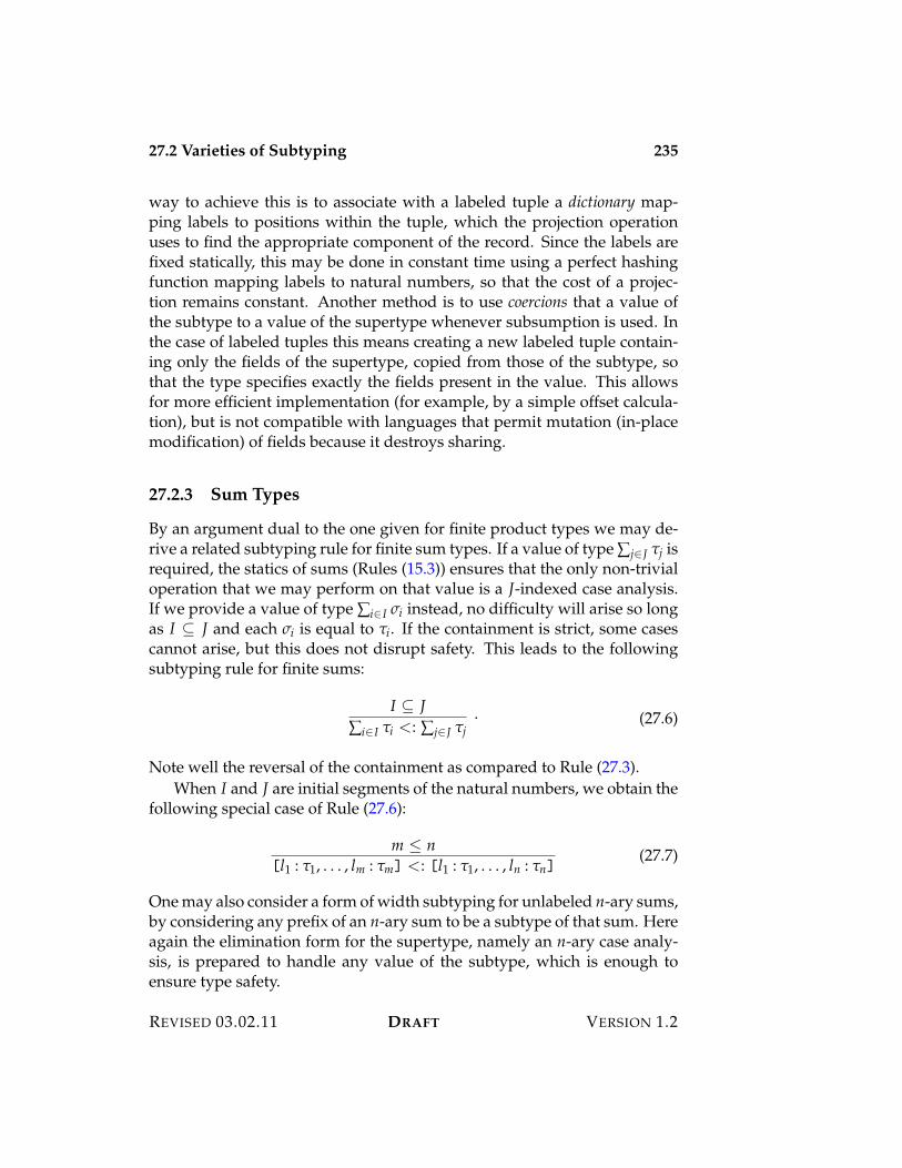
27.2 Varieties of Subtyping 235
way to achieve this is to associate with a labeled tuple a dictionary map-ping labels to positions within the tuple, which the projection operationuses to find the appropriate component of the record. Since the labels arefixed statically, this may be done in constant time using a perfect hashingfunction mapping labels to natural numbers, so that the cost of a projec-tion remains constant. Another method is to use coercions that a value ofthe subtype to a value of the supertype whenever subsumption is used. Inthe case of labeled tuples this means creating a new labeled tuple contain-ing only the fields of the supertype, copied from those of the subtype, sothat the type specifies exactly the fields present in the value. This allowsfor more efficient implementation (for example, by a simple offset calcula-tion), but is not compatible with languages that permit mutation (in-placemodification) of fields because it destroys sharing.
27.2.3 Sum Types
By an argument dual to the one given for finite product types we may de-rive a related subtyping rule for finite sum types. If a value of type 'j+J "j isrequired, the statics of sums (Rules (15.3)) ensures that the only non-trivialoperation that we may perform on that value is a J-indexed case analysis.If we provide a value of type 'i+I &i instead, no difficulty will arise so longas I - J and each &i is equal to "i. If the containment is strict, some casescannot arise, but this does not disrupt safety. This leads to the followingsubtyping rule for finite sums:
I - J'i+I "i <: 'j+J "j
. (27.6)
Note well the reversal of the containment as compared to Rule (27.3).When I and J are initial segments of the natural numbers, we obtain the
following special case of Rule (27.6):
m ( n[l1 : "1, . . . , lm : "m] <: [l1 : "1, . . . , ln : "n]
(27.7)
One may also consider a form of width subtyping for unlabeled n-ary sums,by considering any prefix of an n-ary sum to be a subtype of that sum. Hereagain the elimination form for the supertype, namely an n-ary case analy-sis, is prepared to handle any value of the subtype, which is enough toensure type safety.
REVISED 03.02.11 DRAFT VERSION 1.2
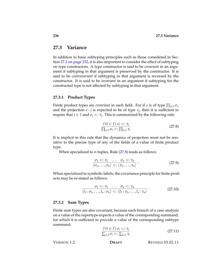
236 27.3 Variance
27.3 Variance
In addition to basic subtyping principles such as those considered in Sec-tion 27.2 on page 232, it is also important to consider the effect of subtypingon type constructors. A type constructor is said to be covariant in an argu-ment if subtyping in that argument is preserved by the constructor. It issaid to be contravariant if subtyping in that argument is reversed by theconstructor. It is said to be invariant in an argument if subtyping for theconstructed type is not affected by subtyping in that argument.
27.3.1 Product Types
Finite product types are covariant in each field. For if e is of type &i+I &i,and the projection e · j is expected to be of type "j, then it is sufficient torequire that j + I and &j <: "j. This is summarized by the following rule:
(&i + I) &i <: "i
&i+I &i <: &i+I "i(27.8)
It is implicit in this rule that the dynamics of projection must not be sen-sitive to the precise type of any of the fields of a value of finite producttype.
When specialized to n-tuples, Rule (27.8) reads as follows:
&1 <: "1 . . . &n <: "n
?&1, . . . , &n@ <: ?"1, . . . , "n@. (27.9)
When specialized to symbolic labels, the covariance principle for finite prod-ucts may be re-stated as follows:
&1 <: "1 . . . &n <: "n
?l1 : &1, . . . , ln : &n@ <: ?l1 : "1, . . . , ln : "n@. (27.10)
27.3.2 Sum Types
Finite sum types are also covariant, because each branch of a case analysison a value of the supertype expects a value of the corresponding summand,for which it is sufficient to provide a value of the corresponding subtypesummand:
(&i + I) &i <: "i
'i+I &i <: 'i+I "i(27.11)
VERSION 1.2 DRAFT REVISED 03.02.11
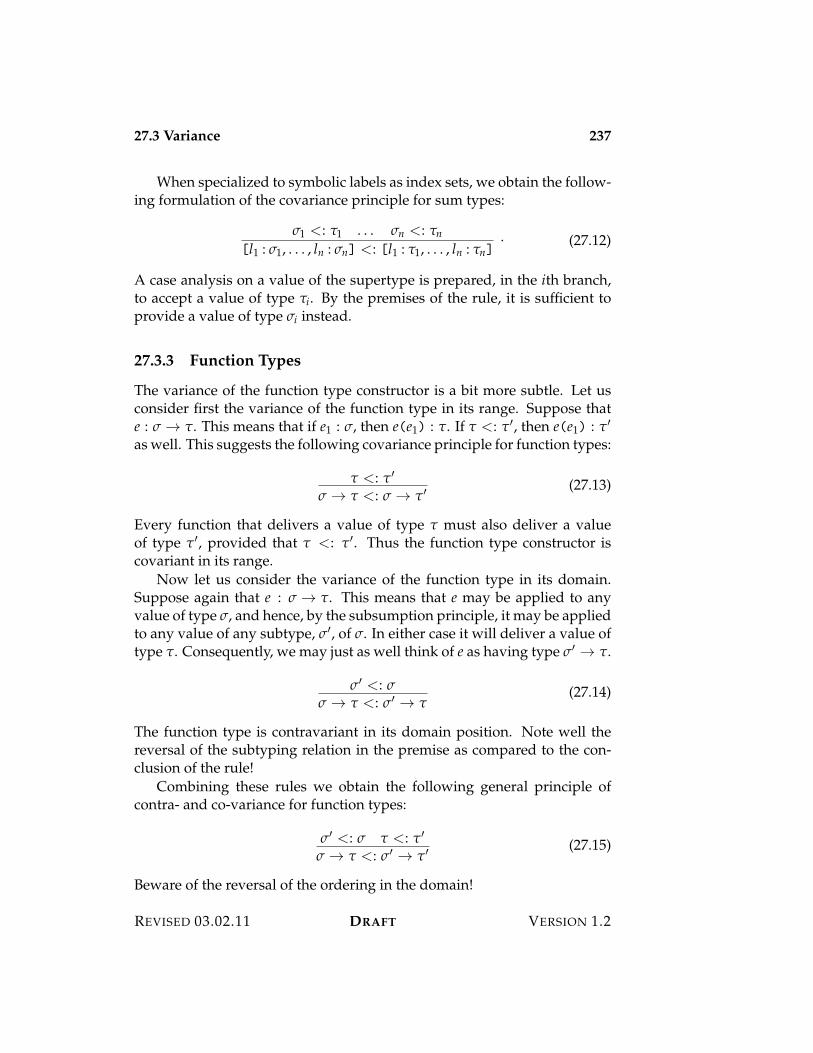
27.3 Variance 237
When specialized to symbolic labels as index sets, we obtain the follow-ing formulation of the covariance principle for sum types:
&1 <: "1 . . . &n <: "n[l1 : &1, . . . , ln : &n] <: [l1 : "1, . . . , ln : "n]
. (27.12)
A case analysis on a value of the supertype is prepared, in the ith branch,to accept a value of type "i. By the premises of the rule, it is sufficient toprovide a value of type &i instead.
27.3.3 Function Types
The variance of the function type constructor is a bit more subtle. Let usconsider first the variance of the function type in its range. Suppose thate : & 3 ". This means that if e1 : &, then e(e1) : ". If " <: "%, then e(e1) : "%
as well. This suggests the following covariance principle for function types:
" <: "%
& 3 " <: & 3 "% (27.13)
Every function that delivers a value of type " must also deliver a valueof type "%, provided that " <: "%. Thus the function type constructor iscovariant in its range.
Now let us consider the variance of the function type in its domain.Suppose again that e : & 3 ". This means that e may be applied to anyvalue of type &, and hence, by the subsumption principle, it may be appliedto any value of any subtype, &%, of &. In either case it will deliver a value oftype ". Consequently, we may just as well think of e as having type &% 3 ".
&% <: && 3 " <: &% 3 "
(27.14)
The function type is contravariant in its domain position. Note well thereversal of the subtyping relation in the premise as compared to the con-clusion of the rule!
Combining these rules we obtain the following general principle ofcontra- and co-variance for function types:
&% <: & " <: "%
& 3 " <: &% 3 "% (27.15)
Beware of the reversal of the ordering in the domain!
REVISED 03.02.11 DRAFT VERSION 1.2
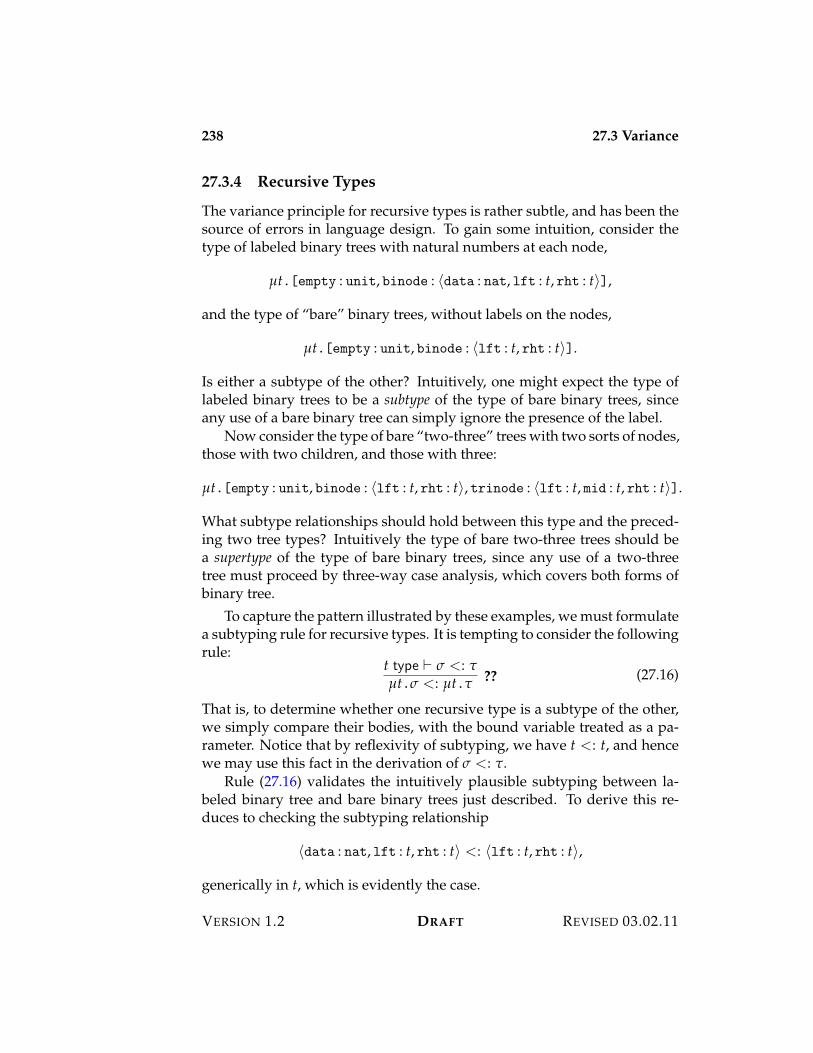
238 27.3 Variance
27.3.4 Recursive Types
The variance principle for recursive types is rather subtle, and has been thesource of errors in language design. To gain some intuition, consider thetype of labeled binary trees with natural numbers at each node,
µt.[empty : unit, binode : ?data : nat, lft : t, rht : t@],
and the type of “bare” binary trees, without labels on the nodes,
µt.[empty : unit, binode : ?lft : t, rht : t@].
Is either a subtype of the other? Intuitively, one might expect the type oflabeled binary trees to be a subtype of the type of bare binary trees, sinceany use of a bare binary tree can simply ignore the presence of the label.
Now consider the type of bare “two-three” trees with two sorts of nodes,those with two children, and those with three:
µt.[empty : unit, binode : ?lft : t, rht : t@, trinode : ?lft : t, mid : t, rht : t@].
What subtype relationships should hold between this type and the preced-ing two tree types? Intuitively the type of bare two-three trees should bea supertype of the type of bare binary trees, since any use of a two-threetree must proceed by three-way case analysis, which covers both forms ofbinary tree.
To capture the pattern illustrated by these examples, we must formulatea subtyping rule for recursive types. It is tempting to consider the followingrule:
t type ) & <: "µt.& <: µt." ?? (27.16)
That is, to determine whether one recursive type is a subtype of the other,we simply compare their bodies, with the bound variable treated as a pa-rameter. Notice that by reflexivity of subtyping, we have t <: t, and hencewe may use this fact in the derivation of & <: ".
Rule (27.16) validates the intuitively plausible subtyping between la-beled binary tree and bare binary trees just described. To derive this re-duces to checking the subtyping relationship
?data : nat, lft : t, rht : t@ <: ?lft : t, rht : t@,
generically in t, which is evidently the case.
VERSION 1.2 DRAFT REVISED 03.02.11
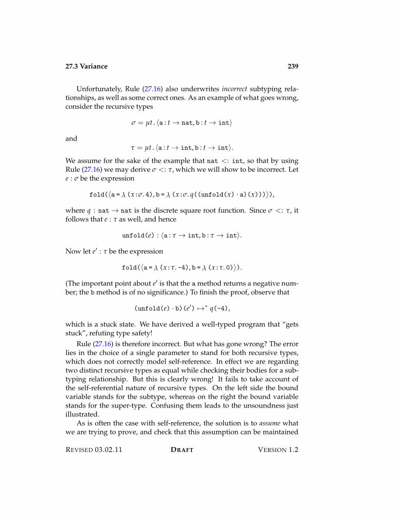
27.3 Variance 239
Unfortunately, Rule (27.16) also underwrites incorrect subtyping rela-tionships, as well as some correct ones. As an example of what goes wrong,consider the recursive types
& = µt.?a : t 3 nat, b : t 3 int@
and" = µt.?a : t 3 int, b : t 3 int@.
We assume for the sake of the example that nat <: int, so that by usingRule (27.16) we may derive & <: ", which we will show to be incorrect. Lete : & be the expression
fold(?a = ! (x:&. 4), b = ! (x:&. q((unfold(x) · a)(x)))@),
where q : nat 3 nat is the discrete square root function. Since & <: ", itfollows that e : " as well, and hence
unfold(e) : ?a : " 3 int, b : " 3 int@.
Now let e% : " be the expression
fold(?a = ! (x:". -4), b = ! (x:". 0)@).
(The important point about e% is that the a method returns a negative num-ber; the b method is of no significance.) To finish the proof, observe that
(unfold(e) · b)(e%) 531 q(-4),
which is a stuck state. We have derived a well-typed program that “getsstuck”, refuting type safety!
Rule (27.16) is therefore incorrect. But what has gone wrong? The errorlies in the choice of a single parameter to stand for both recursive types,which does not correctly model self-reference. In effect we are regardingtwo distinct recursive types as equal while checking their bodies for a sub-typing relationship. But this is clearly wrong! It fails to take account ofthe self-referential nature of recursive types. On the left side the boundvariable stands for the subtype, whereas on the right the bound variablestands for the super-type. Confusing them leads to the unsoundness justillustrated.
As is often the case with self-reference, the solution is to assume whatwe are trying to prove, and check that this assumption can be maintained
REVISED 03.02.11 DRAFT VERSION 1.2
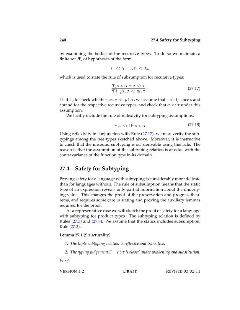
240 27.4 Safety for Subtyping
by examining the bodies of the recursive types. To do so we maintain afinite set, ), of hypotheses of the form
s1 <: t1, . . . , sn <: tn,
which is used to state the rule of subsumption for recursive types:
), s <: t ) & <: ") ) µs.& <: µt."
. (27.17)
That is, to check whether µs.& <: µt.", we assume that s <: t, since s andt stand for the respective recursive types, and check that & <: " under thisassumption.
We tacitly include the rule of reflexivity for subtyping assumptions,
), s <: t ) s <: t (27.18)
Using reflexivity in conjunction with Rule (27.17), we may verify the sub-typings among the tree types sketched above. Moreover, it is instructiveto check that the unsound subtyping is not derivable using this rule. Thereason is that the assumption of the subtyping relation is at odds with thecontravariance of the function type in its domain.
27.4 Safety for Subtyping
Proving safety for a language with subtyping is considerably more delicatethan for languages without. The rule of subsumption means that the statictype of an expression reveals only partial information about the underly-ing value. This changes the proof of the preservation and progress theo-rems, and requires some care in stating and proving the auxiliary lemmasrequired for the proof.
As a representative case we will sketch the proof of safety for a languagewith subtyping for product types. The subtyping relation is defined byRules (27.3) and (27.8). We assume that the statics includes subsumption,Rule (27.2).
Lemma 27.1 (Structurality).
1. The tuple subtyping relation is reflexive and transitive.
2. The typing judgement ! ) e : " is closed under weakening and substitution.
Proof.
VERSION 1.2 DRAFT REVISED 03.02.11
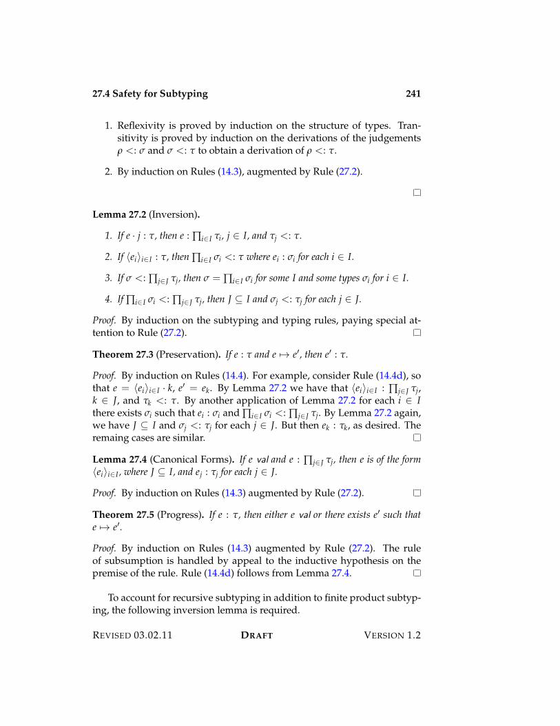
27.4 Safety for Subtyping 241
1. Reflexivity is proved by induction on the structure of types. Tran-sitivity is proved by induction on the derivations of the judgements, <: & and & <: " to obtain a derivation of , <: ".
2. By induction on Rules (14.3), augmented by Rule (27.2).
Lemma 27.2 (Inversion).
1. If e · j : ", then e : &i+I "i, j + I, and "j <: ".
2. If ?ei@i+I : ", then &i+I &i <: " where ei : &i for each i + I.
3. If & <: &j+J "j, then & = &i+I &i for some I and some types &i for i + I.
4. If &i+I &i <: &j+J "j, then J - I and &j <: "j for each j + J.
Proof. By induction on the subtyping and typing rules, paying special at-tention to Rule (27.2).
Theorem 27.3 (Preservation). If e : " and e 53 e%, then e% : ".
Proof. By induction on Rules (14.4). For example, consider Rule (14.4d), sothat e = ?ei@i+I · k, e% = ek. By Lemma 27.2 we have that ?ei@i+I : &j+J "j,k + J, and "k <: ". By another application of Lemma 27.2 for each i + Ithere exists &i such that ei : &i and &i+I &i <: &j+J "j. By Lemma 27.2 again,we have J - I and &j <: "j for each j + J. But then ek : "k, as desired. Theremaing cases are similar.
Lemma 27.4 (Canonical Forms). If e val and e : &j+J "j, then e is of the form?ei@i+I , where J - I, and ej : "j for each j + J.
Proof. By induction on Rules (14.3) augmented by Rule (27.2).
Theorem 27.5 (Progress). If e : ", then either e val or there exists e% such thate 53 e%.
Proof. By induction on Rules (14.3) augmented by Rule (27.2). The ruleof subsumption is handled by appeal to the inductive hypothesis on thepremise of the rule. Rule (14.4d) follows from Lemma 27.4.
To account for recursive subtyping in addition to finite product subtyp-ing, the following inversion lemma is required.
REVISED 03.02.11 DRAFT VERSION 1.2
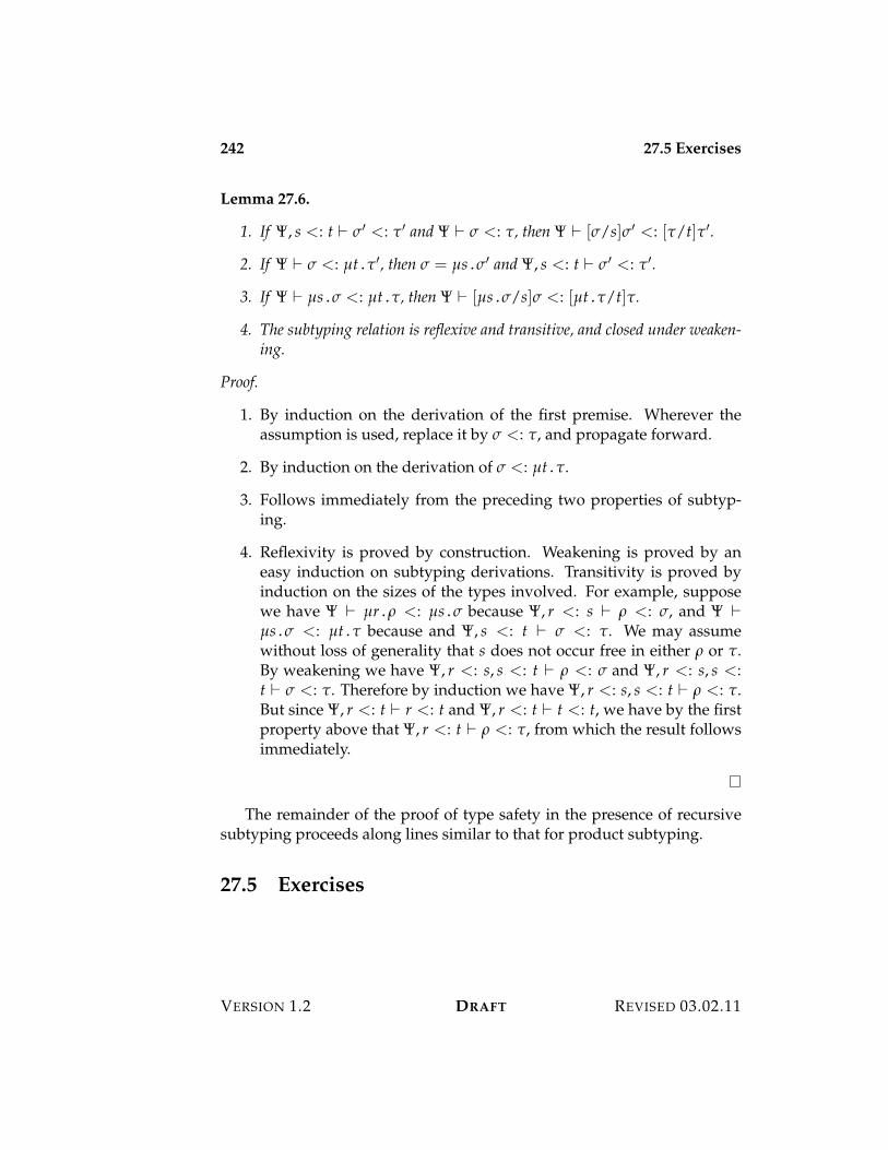
242 27.5 Exercises
Lemma 27.6.
1. If ), s <: t ) &% <: "% and ) ) & <: ", then ) ) [&/s]&% <: ["/t]"%.
2. If ) ) & <: µt."%, then & = µs.&% and ), s <: t ) &% <: "%.
3. If ) ) µs.& <: µt.", then ) ) [µs.&/s]& <: [µt."/t]".
4. The subtyping relation is reflexive and transitive, and closed under weaken-ing.
Proof.
1. By induction on the derivation of the first premise. Wherever theassumption is used, replace it by & <: ", and propagate forward.
2. By induction on the derivation of & <: µt.".
3. Follows immediately from the preceding two properties of subtyp-ing.
4. Reflexivity is proved by construction. Weakening is proved by aneasy induction on subtyping derivations. Transitivity is proved byinduction on the sizes of the types involved. For example, supposewe have ) ) µr., <: µs.& because ), r <: s ) , <: &, and ) )µs.& <: µt." because and ), s <: t ) & <: ". We may assumewithout loss of generality that s does not occur free in either , or ".By weakening we have ), r <: s, s <: t ) , <: & and ), r <: s, s <:t ) & <: ". Therefore by induction we have ), r <: s, s <: t ) , <: ".But since ), r <: t ) r <: t and ), r <: t ) t <: t, we have by the firstproperty above that ), r <: t ) , <: ", from which the result followsimmediately.
The remainder of the proof of type safety in the presence of recursivesubtyping proceeds along lines similar to that for product subtyping.
27.5 Exercises
VERSION 1.2 DRAFT REVISED 03.02.11
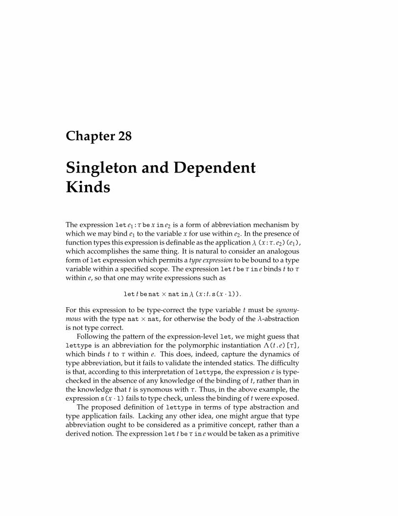
Chapter 28
Singleton and DependentKinds
The expression let e1:" be x in e2 is a form of abbreviation mechanism bywhich we may bind e1 to the variable x for use within e2. In the presence offunction types this expression is definable as the application ! (x:". e2)(e1),which accomplishes the same thing. It is natural to consider an analogousform of let expression which permits a type expression to be bound to a typevariable within a specified scope. The expression let t be " in e binds t to "within e, so that one may write expressions such as
let t be nat< nat in! (x:t. s(x · l)).
For this expression to be type-correct the type variable t must be synony-mous with the type nat< nat, for otherwise the body of the !-abstractionis not type correct.
Following the pattern of the expression-level let, we might guess thatlettype is an abbreviation for the polymorphic instantiation ((t.e)["],which binds t to " within e. This does, indeed, capture the dynamics oftype abbreviation, but it fails to validate the intended statics. The difficultyis that, according to this interpretation of lettype, the expression e is type-checked in the absence of any knowledge of the binding of t, rather than inthe knowledge that t is synomous with ". Thus, in the above example, theexpression s(x · l) fails to type check, unless the binding of t were exposed.
The proposed definition of lettype in terms of type abstraction andtype application fails. Lacking any other idea, one might argue that typeabbreviation ought to be considered as a primitive concept, rather than aderived notion. The expression let t be " in e would be taken as a primitive
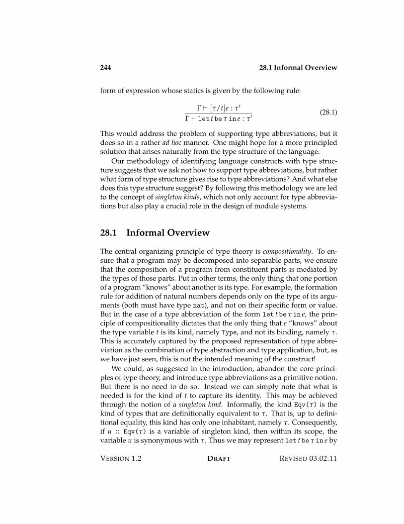
244 28.1 Informal Overview
form of expression whose statics is given by the following rule:
! ) ["/t]e : "%
! ) let t be " in e : "% (28.1)
This would address the problem of supporting type abbreviations, but itdoes so in a rather ad hoc manner. One might hope for a more principledsolution that arises naturally from the type structure of the language.
Our methodology of identifying language constructs with type struc-ture suggests that we ask not how to support type abbreviations, but ratherwhat form of type structure gives rise to type abbreviations? And what elsedoes this type structure suggest? By following this methodology we are ledto the concept of singleton kinds, which not only account for type abbrevia-tions but also play a crucial role in the design of module systems.
28.1 Informal Overview
The central organizing principle of type theory is compositionality. To en-sure that a program may be decomposed into separable parts, we ensurethat the composition of a program from constituent parts is mediated bythe types of those parts. Put in other terms, the only thing that one portionof a program “knows” about another is its type. For example, the formationrule for addition of natural numbers depends only on the type of its argu-ments (both must have type nat), and not on their specific form or value.But in the case of a type abbreviation of the form let t be " in e, the prin-ciple of compositionality dictates that the only thing that e “knows” aboutthe type variable t is its kind, namely Type, and not its binding, namely ".This is accurately captured by the proposed representation of type abbre-viation as the combination of type abstraction and type application, but, aswe have just seen, this is not the intended meaning of the construct!
We could, as suggested in the introduction, abandon the core princi-ples of type theory, and introduce type abbreviations as a primitive notion.But there is no need to do so. Instead we can simply note that what isneeded is for the kind of t to capture its identity. This may be achievedthrough the notion of a singleton kind. Informally, the kind Eqv(") is thekind of types that are definitionally equivalent to ". That is, up to defini-tional equality, this kind has only one inhabitant, namely ". Consequently,if u :: Eqv(") is a variable of singleton kind, then within its scope, thevariable u is synonymous with ". Thus we may represent let t be " in e by
VERSION 1.2 DRAFT REVISED 03.02.11
28.1 Informal Overview 245
((t::Eqv(").e)["], which correctly propagates the identity of t, namely", to e during type checking.
A proper treatment of singleton kinds requires some additional machin-ery at the constructor and kind level. First, we must capture the idea thata constructor of singleton kind is a fortiori a constructor of kind Type, andhence is a type. Otherwise, a variable, u, singleton kind cannot be used asa type, even though it is explicitly defined to be one! This may be capturedby introducing a subkinding relation, .1 :<: .2, which is analogous to sub-typing, exception at the kind level. The fundamental axiom of subkindingis Eqv(") :<: Type, stating that every constructor of singleton kind is atype.
Second, we must account for the occurrence of a constructor of kindType within the singleton kind Eqv("). This intermixing of the construc-tor and kind level means that singletons are a form of dependent kind inthat a kind may depend on a constructor. Another way to say the samething is that Eqv(") represents a family of kinds indexed by constructors ofkind Type. This, in turn, implies that we must generalize the function andproduct kinds to dependent functions and dependent products. The dependentfunction kind, * u::.1..2 classifies functions that, when applied to a con-structor c1 :: .1, results in a constructor of kind [c1/u].2. The importantpoint is that the kind of the result is sensitive to the argument, and notjust to its kind.1 The dependent product kind, $ u::.1..2, classifies pairs?c1, c2@ such that c1 :: .1, as might be expected, and c2 :: [c1/u].2, in whichthe kind of the second component is sensitive to the first component itself,and not just its kind.
Third, it is useful to consider singletons not just of kind Type, but alsoof higher kinds. To support this we introduce higher-kind singletons, writtenEqv(c::.), where . is a kind and c is a constructor of kind k. These aredefinable in terms of the primitive form of singleton kind by making use ofdependent function and product kinds.
This chapter is under construction . . . .
1As we shall see in the development, the propagation of information as sketched here ismanaged through the use of singleton kinds.
REVISED 03.02.11 DRAFT VERSION 1.2
246 28.1 Informal Overview
VERSION 1.2 DRAFT REVISED 03.02.11
Part X
Classes and Methods

Chapter 29
Dynamic Dispatch
It frequently arises that the values of a type are partitioned into a variety ofclasses, each classifying data with distinct internal structure. A good exam-ple is provided by the type of points in the plane, which may be classifiedaccording to whether they are represented in cartesian or polar form. Bothare represented by a pair of real numbers, but in the cartesian case theseare the x and y coordinates of the point, whereas in the polar case theseare its distance, ,, from the origin and its angle, *, with the polar axis. Aclassified value is said to be an instance of, or an object of its class. The classdetermines the type of the classified data, which is called the instance typeof the class. The classified data itself is called the instance data of the object.
Functions that act on classified values are called methods. The behaviorof a method is determined by the class of its argument. The method is saidto dispatch on the class of the argument. Because it happens at run-time,this is called, rather grandly, dynamic dispatch. For example, the distanceof a point from the origin is calculated differently according to whetherthe point is represented in cartesian or polar form. In the former case therequired distance is
*x2 + y2, whereas in the latter it is simply , itself. Sim-
ilarly, the quadrant of a cartesian point may be determined by examiningthe sign of its x and y coordinates, and the quadrant of a polar point maybe calculated by taking the integral part of the angle * divided by #/2.
Since each method acts by dispatch on the class of its argument, we mayenvision the entire system of classes and methods as a matrix, edm, calledthe dispatch matrix, whose rows are classes, whose columns are methods,and whose (c, d)-entry is the code for method d acting on an argument ofclass c, expressed as a function of the instance data of the object. Thus, the
250
dispatch matrix has a type of the form
&c+C
&d+D
(&c 3 ,d),
where C is the set of class names, D is the set of method names, &c is theinstance type associated with class c and ,d is the result type of method d.The instance type is the same for all methods acting on a given class, andthat the result type is the same for all classes acted on by a given method.
There are two main ways to organize a system of classes and methods,according to whether we wish to place emphasis on the classes, thoughtof as a collection of methods acting on its instances, or on the methods,thought of as a collection of classes on which the methods act. These are,respectively, the class-based and the method-based organizations. Languagesthat place special emphasis on classes and methods, called object-orientedlanguages,1 usually adopt one or the other of these organizations as a centraldesign principle.
There is little point in making heavy weather of the distinction, bothbeing applicable in different situations. What is important is that both arisefrom simple manipulations of the dispatch matrix based on symmetries be-tween product and sum types. A fully expressive language supports sumsand products equally well, and hence supports the class-based organiza-tion as readily as the method-based, rather than taking a doctrinal stancethat cannot be maintained in the face of these symmetries.
The method-based organization starts with the transpose of the dispatchmatrix, which has the type
&d+D
&c+C
(&c 3 ,d).
By observing that each row of the transposed dispatch matrix determines amethod, we obtain the method vector, emv, of type
"mv % &d+D
('c+C
&c) 3 ,d.
Each entry of the method vector consists of a dispatcher that determines theresult as a function of the instance data associated with a given object. Thisorganization makes it easy to add new methods for a given collection ofclasses by simply defining a new function of this type. It makes adding a
1The term “object-oriented” itself speaks to the vagueness of the concept. It is used, forthe most part, to express approval.
VERSION 1.2 DRAFT REVISED 03.02.11
29.1 The Dispatch Matrix 251
new class relatively more difficult, however, since doing so requires thateach method be updated to account for the new forms of object.
The class-based organization starts with the observation that the dis-patch matrix may be reorganized to “factor out” the instance data for eachmethod acting on that class to obtain the class vector, ecv, of type
"cv % &c+C
(&c 3 (&d+D
,d)).
Each row of the class vector consists of a constructor that determines theresult of each of the methods when acting on given instance data. Thisorganization makes it easy to add a new class to the program; we needonly define the method tuple on the instance data for the new class. Itmakes adding a new method relatively more difficult, however, becausewe must extend the interpretation of each class to account for it.
We will show how to give a method-based and a class-based implemen-tation of objects by defining the following concepts:
• The type of objects arising as instances of the classes on which themethods act.
• The operation new[c](e) that creates an object of the class c with in-stance data given by the expression e.
• The operation eJ d that invokes method d on the instance given bythe expression e.
Informally, under the method-based organization an object consists of theinstance data tagged with its class. A new instance is created by attachingthe class tag to the instance data, and a method is invoked by dispatchingon the class of the instance. Conversely, under the class-based organizationan object consists of a tuple of results of each of the methods acting on theinstance data of the object. A new object is created by applying each of themethods to given instance data, and a method is invoked by projecting theresult from the object.
29.1 The Dispatch Matrix
As an illustrative example, let us consider the type of points in the planeclassified into two classes, cart and pol, corresponding to the cartesian
REVISED 03.02.11 DRAFT VERSION 1.2
252 29.1 The Dispatch Matrix
and polar representations. The instance data for a cartesian point has thetype
&cart = ?x : real, y : real@,
and the instance data for a polar point has the type
&pol = ?r : real, th : real@.
Consider two methods acting on points, dist and quad, which com-pute, respectively, the squared distance of a point from the origin and thequadrant of a point. The distance method is given by the tuple edist =?cart = ecartdist, pol = epoldist@ of type
?cart : &cart 3 ,dist, pol : &pol 3 ,dist@,
where ,dist = real is the result type,
ecartdist = ! (u:&cart. (u · x)2 + (u · y)2)
is the distance computation for a cartesian point, and
epoldist = ! (v:&pol. (v · r)2)
is the distance computation for a polar point. Similarly, the quadrant methodis given by the tuple equad = ?cart = ecartquad, pol = epolquad@ of type
?cart : &cart 3 ,quad, pol : &pol 3 ,quad@,
where ,quad = [I, II, III, IV] is the type of quadrants, and ecartquad and epolquad
are expressions that compute the quadrant of a point in rectangular andpolar forms, respectively.
Now let C = { cart, pol } and let D = { dist, quad }, and define thedispatch matrix, edm, to be the value of type
&c+C
&d+D
(&c 3 ,d)
such that, for each class c and method d,
edm · c · d 531 ecd.
That is, the entry in the dispatch matrix, edm, for class c and method d isdefined to be the implementation of that method acting on an instance ofthat class.
VERSION 1.2 DRAFT REVISED 03.02.11
29.2 Method-Based Organization 253
29.2 Method-Based Organization
An object is a value of type & = 'c+C &c, the sum over the classes of theinstance types. For example, the type of points in the plane is the sum type
[cart : &cart, pol : &pol].
Each point is labelled with its class, specifying its representation as havingeither cartesian or polar form.
An instance of a class c is just the instance data labelled with its class toform an element of the object type:
new[c](e) % c · e.
For example, a cartesian point with coordinates x0 and y0 is given by theexpression
new[cart](?x = x0, y = y0@) % cart · ?x = x0, y = y0@.
Similarly, a polar point with distance ,0 and angle *0 is given by the expres-sion
new[pol](?r = r0, th = *0@) % pol · ?r = r0, th = *0@.
The method-based organization consolidates the implementation of eachmethod into the method vector, emv of type "mv, defined by ?ed@d+D, wherefor each d + D the expression ed : & 3 ,d is
! (this:&. case this {c · u ; edm · c · d(u)}c+C).
Each entry in the method vector may be thought of as a dispatch functionthat determines the action of that method on each class of object.
In the case of points in the plane, the method vector has the producttype
?dist : & 3 ,dist, quad : & 3 ,quad@.
The dispatch function for the dist method has the form
! (this:&. case this {cart · u ; edm · cart · dist(u) | pol · v ; edm · pol · dist(v)}),
and the dispatch function for the quad method has the similar form
! (this:&. case this {cart · u ; edm · cart · quad(u) | pol · v ; edm · pol · quad(v)}).
REVISED 03.02.11 DRAFT VERSION 1.2
254 29.3 Class-Based Organization
The message send operation, eJ d, applies the dispatch function for methodd to the object e:
eJ d % emv · d(e).
Thus we have, for each class, c, and method, d,
(new[c](e))J d 531 emv · d(c · e)531 edm · c · d(e)
That is, the message send invokes the implementation of the method d onthe instance data for the given object.
29.3 Class-Based Organization
An object has the type , = &d+D ,d consisting of the product over themethods of the result types of the methods. For example, in the case ofpoints in the plane, the type , is the product type
?dist : ,dist, quad : ,quad@.
Each component specifies the result of each of the methods acting on thatobject.
The message send operation, eJ d, is just the projection e · d. So, in thecase of points in the plane, eJ dist is the projection e · dist, and similarlyeJ quad is the projection e · quad.
The class-based organization consolidates the implementation of eachclass into a class vector, ecv, a tuple of type "cv consisting of the constructorof type &c 3 , for each class c + C. The class vector is defined by ecv =?ec@c+C, where for each c + C the expression ec is
! (u:&c. ?edm · c · d(u)@d+D).
For example, the constructor for the class cart is the function ecartgiven by the expression
! (u:&cart. ?dist = edm · cart · dist(u), quad = edm · cart · quad(u)@).
Similarly, the constructor for the class pol is the function epol given by theexpression
! (u:&pol. ?dist = edm · pol · dist(u), quad = edm · pol · quad(u)@).
VERSION 1.2 DRAFT REVISED 03.02.11
29.4 Self-Reference 255
The class vector, ecv, in this case is the tuple ?cart = ecart, pol = epol@ of type?cart : &cart 3 ,, pol : &pol 3 ,@.
An instance of a class is obtained by applying the constructor for thatclass to the instance data:
new[c](e) % ecv · c(e).
For example, a cartesian point is obtained by writing new[cart](?x = x0, y = y0@),which is defined by the expression
ecv · cart(?x = x0, y = y0@).
Similarly, a polar point is obtained by writing new[pol](r = r0, th = *0),which is defined by the expression
ecv · pol(?r = r0, th = *0@).
It is easy to check for this organization of points that for each class c andmethod d, we may derive
(new[c](e))J d 531 (ecv · c(e)) · d531 edm · c · d(e)
The outcome is, of course, the same as for the method-based organization.
29.4 Self-Reference
A significant shortcoming of the foregoing account of classes and methodsis that methods are not permitted to create new objects or to send messagesto existing objects. The elements of the dispatch matrix are functions whosedomain and range are given in advance. It is only after the dispatch ma-trix has been defined that we are able to choose either the method-basedor class-based organization for computing with classified objects. Rectify-ing this will, en passant, also permit methods to call one another, perhapseven themselves, and allow constructors to create instances, perhaps evenof their own class.
The first step to correcting this shortcoming is to change the definitionand type of the dispatch matrix so that method bodies may create instancesand send messages. This is not quite so straightforward as it may sound,because the meaning of instance creation and message send varies accord-ing to whether we are using a method-based or a class-based organization.
REVISED 03.02.11 DRAFT VERSION 1.2
256 29.4 Self-Reference
Naıvely, this would seem to imply that the dispatch matrix can no longerbe organized along either the method or class axis, but must instead bedefined separately according to whether we are using a method-based orclass-based organization. However, the dependency can be avoided by us-ing an abstract type to avoid representation commitments.
To allow methods to call one another and to allow constructors to gen-erate objects of other classes, the types of the class and method vectorsmust be given self-referential types (see Section 19.3 on page 161). This isnecessary because the definitions of message send (in the method-basedsetup) and instantiation (in the class-based setup) imply that the dispatch-ers in the method vector and the constructors in the class vector may referto themselves indirectly via the dispatch matrix.
The type of the dispatch matrix is generalized to the polymorphic type
&c+C
&d+D
&(t."cv 3 "mv 3 &c 3 ,d),
where t is the abstract type of objects, the type of the class vector is givenby the equation
"cv = &c+C
(&c 3 t),
and the type of the method vector is given by the equation
"mv = (&d+D
t 3 ,d).
Each class vector entry is a constructor yielding an object of type t giveninstance data for that class, and each method vector entry is a dispatcherthat acts on an object of type t to determine the result of that method. Theentry for class c and method d in the dispatch matrix has the form
((t.! (cv:"cv. ! (mv:"mv. ! (u:&c. e)))),
where within the body e a new object of class c% with instance data e% is ob-tained by writing cv · c%(e%), and a message d% is sent to an object e% by writ-ing mv · d%(e%). Thus the implementation of method d on class c may createan instance of any class, including c itself, and may invoke any method,including d itself.
The change to the type of the dispatch matrix requires that we recon-sider the definition of the class and method vectors. Under the method-based organization the instantiation operation is defined directly to tag theinstance data with its class, just as before. The messaging operation must
VERSION 1.2 DRAFT REVISED 03.02.11
29.5 Exercises 257
be generalized, however, to allow for the self-reference engendered by in-voking a method that may itself invoke another method. Dually, underthe class-based organizaton messaging is defined by projection, as before,but instantiation must be generalized to to account for the self-referenceengendered by a constructor creating an instance.
To allow for self-reference the method vector, emv is defined to have thetype [&/t]"mv self, in which the abstract object type is specialized to thesum over all classes of their instance types. The method vector is definedby the expression
selfmv is ?d = ! (this:&. case this {c · u ; edm · c · d[&](e%cv)(e%mv)(u)}c+C)@d+D,
where the class vector argument, e%cv, is the tuple of tagging operations?c = ! (u:&c. c · u)@c+C, and the method vector argument, e%mv, is the recur-sive unrolling of the method vector itself, unroll(mv). The message sendoperation eJ d is given by the expression unroll(emv) · d(e), whereas ob-jection creation, new[c](e), is defined as before to be c · e.
Alternatively, under the class-based organization, the class vector, ecv,is defined to have the type [,/t]"cv self, which specifies that the abstracttype of objects is the product over all methods of their result types. Theclass vector itself is given by the expression
self cv is ?c = ! (u:&c. ?d = edm · c · d[,](e%%cv)(e%%mv)(u)@d+D)@c+C
where the class vector argument, e%%cv, is unroll(cv), and the method vec-tor argument, e%%mv, is the tuple of projections, ?d = ! (this:,. this · d)@d+D.Object creation, new[c](e) is defined by the expression unroll(ecv) · c(e),whereas message send, dJ e, is defined, as before, by e · d.
The symmetries between the two organizations are striking; they reflectthe duality between sum and product types.
29.5 Exercises
1. Generalize the class-based table to allow each class to determine theset of methods defined on it, and similarly generalize the method-based table to allow each method to act on certain classes.
2. Extend to allow methods to return instances as results and construc-tors to take instances as arguments. The method-based approach hasno difficulty with the former, but requires some modification to allowfor the latter; dually, the class-based approach has no difficulty withthe latter, but requires some modification to allow for the former.
REVISED 03.02.11 DRAFT VERSION 1.2
258 29.5 Exercises
3. Add support for an instance test, which allows testing whether an ob-ject is an instance of a specified class. This amounts to insisting thateach object come equipped with a family of methods instanceof[c],where c + C, which evaluates to a boolean according to whether theobject is an instance of class c or not.
VERSION 1.2 DRAFT REVISED 03.02.11
Chapter 30
Inheritance
Dynamic dispatch was introduced in Chapter 29 as a means of organizingthe action of a collection of methods on instances of a collection of classes.The dispatch matrix assigns to each class, c, and each method, d, an im-plementation of type &c 3 ,d mapping the instance data appropriate forclass c to a result appropriate for method d. In this chapter we consider theproblem of building up the dispatch matrix by extending it with either anew class or a new method (or both) using inheritance. The main idea is tosupport code reuse by defining a new class or a new method by inheritingmuch of the implementation from one or more existing classes or methods,but allowing for modifications, called overrides, that alter the behavior ofthe new class or method. Methodologically speaking, these modificationsare intended to be relatively few compared to the full extent of the imple-mentation, but nothing precludes a wholesale redefinition of the behaviorof the new class or method compared to the old one. Consequently, know-ing that one class or method inherits from another tells us nothing about thebehavior of the child compared to that of the parent(s).1
In this chapter we will consider the most common form of inheritance,called subclassing, which is defined for the class-based organization de-scribed in Chapter 29. We are given a class vector, ecv, and we are to definea new class vector, e1cv, by adding a subclass, c1 of the superclasses c1, . . . , cn,where n 7 0. A dual form of inheritance, for which there is no establishedterminology but which one might call submethoding, may be defined for themethod-based organization given in Chapter 29. We will not develop thisidea in detail here, but rather leave it as an exercise for the reader.
1In view of this one may doubt the significance of programming methodologies thatstress inheritance as a central organizing principle.
260 30.1 Subclassing
It is common to distinguish two forms of inheritance, single inheritance,which restricts the number, n, of superclasses or supermethods to 1, andmultiple inheritance, which places no limit on n. Single inheritance is better-behaved in that each child class or method has a unique parent. Multipleinheritance introduces ambiguities when there is more than one superclassproviding a method or class that is inherited by the child. Consequently, arule is required to determine from which parent a given attribute is to beinherited.
Inheritance is often confused with subtyping. Whereas inheritance issimply a statement about how a body of code came into being, subtypingis a statement about how a body of code can be expected to behave. Manylanguages seek to ensure that if one class inherits from another, then thetype of objects of the subclass is a subtype of the type of objects of thesuperclass. As we shall see, this is not automatically the case.
30.1 Subclassing
We begin with the class-based organization described in Chapter 29. Letecv : (&c+C &c 3 &d+D ,d) be a class vector, and suppose that c1, . . . , cn +C. Defining a subclass, c1 /+ C, of the superclasses c1, . . . , cn, consists ofspecifying the following information:
1. The instance type &c1 of the new class such that &c1 <: &ci for each1 ( i ( n.
2. The subset Dinh - D of inherited methods. The remaining set Dovr =D \ Dinh is defined to be the set of overridden methods.
3. For each d + Dovr, an expression ed : &c1 3 ,d, the action of the over-ridden method, d, on instances of the class c1.
By the principles of co- and contravariance for function types (see Chap-ter 27) the domain type of the expression ed may be a supertype of &c1 andits range type may be a subtype of ,d.
Given this data, the extended class vector, e1cv, is defined as follows:
1. For each class c + C, the constructor e1cv · c is equivalent to the con-structor ecv · c. That is, all existing classes are preserved intact.
2. The action of the method d on an instance of class c1 is defined asfollows:
VERSION 1.2 DRAFT REVISED 03.02.11
30.1 Subclassing 261
(a) If d + Dinh is an inherited method, then, for some 1 ( i ( nand any instance data e0 of type &c1 , the method e1cv · c1(e0) · d isequivalent to the method e1cv · ci(e0) · d. (When n 7 2 the choiceof i must be given by some fixed rule, which we do not specifyhere.)
(b) If d + Dovr is an overridden method, then for any instance datae0 of type &c1 , the method e1cv · c1(e0) · d is equivalent to ed(e0),where ed is given by the subclass definition.
The resulting class vector, e1cv, is of type
&c+C*{ c1 }
(&c 3 &d+D
,d).
The requirement that &c1 <: &ci ensures that the instance data for the sub-class may be acted upon by a method of the superclass. The condition oninherited methods ensures that the message new[c1](e0)J d is equivalentto the message new[ci](e0)J d, and the condition on overridden methodsensure that new[c1](e0)J d is equivalent to ed(e0).
In this simple formulation of the class vector the object type , = &d+D ,dis unaffected by inheritance. A more sophisticated formulation of the classvector allows each class to determine the methods supported by objects ofthat class, and allows the result types of these methods to vary with theclass. Specifically, let us generalize the set, D, of methods into a family ofsets { Dc }c+C, with Dc being the methods supported by objects of class c.Additionally, for each c + C and each d + Dc let the result type, ,c
d, ofmethod d acting on instances of class c be given. The class vector then hasthe type
&c+C
&c 3 ( &d+Dc
,cd).
The object type, ,c = &d+Dc ,cd, is the type of instances of class c.2
Given a class vector, ecv, of the above type, a subclass c1 of superclassesc1, . . . , cn is defined by specifying the following information:
1. The instance type, &c1 , for the new class such that &c1 <: &ci for each1 ( i ( n.
2. The set Dc1 = Dinh K Dovr K Dext of inherited, overridden, and ex-tending methods associated with class c1 such that Dinh K Dovr -+
1(i(n Dci .2In many accounts the type ,c is identified with the class c, thereby confusing classes with
types.
REVISED 03.02.11 DRAFT VERSION 1.2
262 30.1 Subclassing
3. For each d + Dovr K Dext, an expression ed : &c1 3 ,c1d providing the
implementation of method d for the new class c1.
Since each class determines its own collection of methods, we now requirethat Dci 0 Dcj = # whenever i ,= j, so that no method is provided by morethan one superclass.
This data determines a new class vector, e1cv, defined as follows:
1. For each class c + C, the constructor e1cv · c is equivalent to the con-structor ecv · c.
2. The action of the method d on an instance of class c1 is defined asfollows:
(a) If d + Dinh is an inherited method, then, for a unique 1 ( i ( nand any instance data e0 of type &c1 , the method e1cv · c1(e0) · d isequivalent to the method e1cv · ci(e0) · d.
(b) If d + Dovr K Dext is an overridden or extending method, thenfor any instance data e0 of type &c1 , the method e1cv · c1(e0) · d isequivalent to ed(e0), where ed is given by the subclass definition.
There is no longer any ambiguity in the choice of inherited methods, sincethe superclass method suites are assumed to be disjoint.
The resulting class vector has type
&c+CK{c1}
(&c 3 ( &d+Dc
,cd)).
Letting ,c = &d+Dc ,cd be the object type associated to class c, observe that
the subclass object type, ,c1 , need not be a subtype of any superclass objecttype, ,ci . That is, inheritance does not imply subtyping. For example, thesubclass result type of an overriding method need not bear any relationshipto any superclass result type for that method. Moreover, the subclass neednot provide all of the methods provided by the superclasses. However, ifwe impose the additional requirements that (1) if d + Dovr, then ,c1
d <: ,cid
for the unique superclass ci providing the method d, and (2) Dinh K Dovr =+1(i(n Dci , then the type of subclass objects will be a subtype of the object
types of the superclasses. Consequently, a subclass object may be usedwherever a superclass object is required. Many object-oriented languagesinsist on this condition as a constraint on inheritance. However, this policyis not always sustainable. Certain advanced forms of inheritance3 preclude
3Namely, those involving “self types, ” which we do not consider here.
VERSION 1.2 DRAFT REVISED 03.02.11
30.2 Exercises 263
this policy. Fundamentally, inheritance and subtyping are two differentconcepts. Whereas subtyping is, by the subsumption principle, a matterof essence, inheritance, being only an artifact of how a body of code wascreated is a matter of accident.
30.2 Exercises
1. Extend inheritance to self-referential methods.
2. Develop the idea of submethoding for the method-based organization.Given a method vector, emv, we are to define a new method vector,e1mv, extended with a submethod, d1, of the supermethods, d1, . . . , dn,where n 7 0.
3. Allow overlaps among the superclasses provided that all such meth-ods are overridden in the subclass so that there can be no ambiguity.
REVISED 03.02.11 DRAFT VERSION 1.2

264 30.2 Exercises
VERSION 1.2 DRAFT REVISED 03.02.11

Part XI
Control Effects

Chapter 31
Control Stacks
The technique of structural dynamics is very useful for theoretical pur-poses, such as proving type safety, but is too high level to be directly usablein an implementation. One reason is that the use of “search rules” requiresthe traversal and reconstruction of an expression in order to simplify onesmall part of it. In an implementation we would prefer to use some mecha-nism to record “where we are” in the expression so that we may “resume”from that point after a simplification. This can be achieved by introduc-ing an explicit mechanism, called a control stack, that keeps track of thecontext of an instruction step for just this purpose. By making the controlstack explicit the transition rules avoid the need for any premises—everyrule is an axiom. This is the formal expression of the informal idea that notraversals or reconstructions are required to implement it. In this chapterwe introduce an abstract machine, K{nat"}, for the language L{nat"}.The purpose of this machine is to make control flow explicit by introducinga control stack that maintains a record of the pending sub-computations ofa computation. We then prove the equivalence of K{nat"} with the struc-tural dynamics of L{nat"}.
31.1 Machine Definition
A state, s, of K{nat"} consists of a control stack, k, and a closed expression,e. States may take one of two forms:
1. An evaluation state of the form k $ e corresponds to the evaluation ofa closed expression, e, relative to a control stack, k.
268 31.1 Machine Definition
2. A return state of the form k # e, where e val, corresponds to the evalu-ation of a stack, k, relative to a closed value, e.
As an aid to memory, note that the separator “points to” the focal entityof the state, the expression in an evaluation state and the stack in a returnstate.
The control stack represents the context of evaluation. It records the“current location” of evaluation, the context into which the value of thecurrent expression is to be returned. Formally, a control stack is a list offrames:
% stack (31.1a)
f frame k stack
k; f stack(31.1b)
The definition of frame depends on the language we are evaluating. Theframes of K{nat"} are inductively defined by the following rules:
s($) frame (31.2a)
ifz($; e1; x.e2) frame (31.2b)
ap($; e2) frame (31.2c)
The frames correspond to rules with transition premises in the dynamicsof L{nat"}. Thus, instead of relying on the structure of the transitionderivation to maintain a record of pending computations, we make an ex-plicit record of them in the form of a frame on the control stack.
The transition judgement between states of the K{nat"} is inductivelydefined by a set of inference rules. We begin with the rules for naturalnumbers.
k $ z 53 k # z (31.3a)
k $ s(e) 53 k;s($) $ e (31.3b)
k;s($) # e 53 k # s(e) (31.3c)
To evaluate z we simply return it. To evaluate s(e), we push a frame onthe stack to record the pending successor, and evaluate e; when that returnswith e%, we return s(e%) to the stack.
Next, we consider the rules for case analysis.
k $ ifz(e; e1; x.e2) 53 k;ifz($; e1; x.e2) $ e (31.4a)
k;ifz($; e1; x.e2) # z 53 k $ e1 (31.4b)
VERSION 1.2 DRAFT REVISED 03.02.11
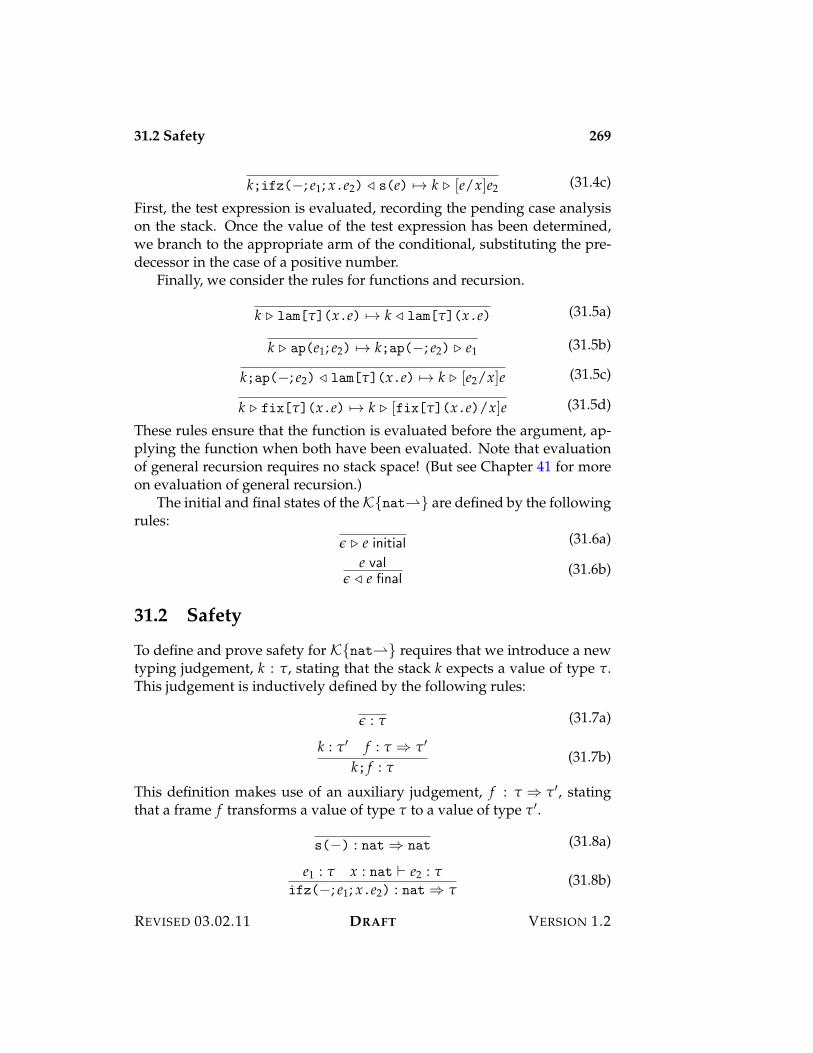
31.2 Safety 269
k;ifz($; e1; x.e2) # s(e) 53 k $ [e/x]e2 (31.4c)
First, the test expression is evaluated, recording the pending case analysison the stack. Once the value of the test expression has been determined,we branch to the appropriate arm of the conditional, substituting the pre-decessor in the case of a positive number.
Finally, we consider the rules for functions and recursion.
k $ lam["](x.e) 53 k # lam["](x.e) (31.5a)
k $ ap(e1; e2) 53 k;ap($; e2) $ e1 (31.5b)
k;ap($; e2) # lam["](x.e) 53 k $ [e2/x]e (31.5c)
k $ fix["](x.e) 53 k $ [fix["](x.e)/x]e (31.5d)
These rules ensure that the function is evaluated before the argument, ap-plying the function when both have been evaluated. Note that evaluationof general recursion requires no stack space! (But see Chapter 41 for moreon evaluation of general recursion.)
The initial and final states of the K{nat"} are defined by the followingrules:
% $ e initial (31.6a)
e val% # e final (31.6b)
31.2 Safety
To define and prove safety for K{nat"} requires that we introduce a newtyping judgement, k : ", stating that the stack k expects a value of type ".This judgement is inductively defined by the following rules:
% : " (31.7a)
k : "% f : " ; "%
k; f : "(31.7b)
This definition makes use of an auxiliary judgement, f : " ; "%, statingthat a frame f transforms a value of type " to a value of type "%.
s($) : nat ; nat (31.8a)
e1 : " x : nat ) e2 : "ifz($; e1; x.e2) : nat ; "
(31.8b)
REVISED 03.02.11 DRAFT VERSION 1.2
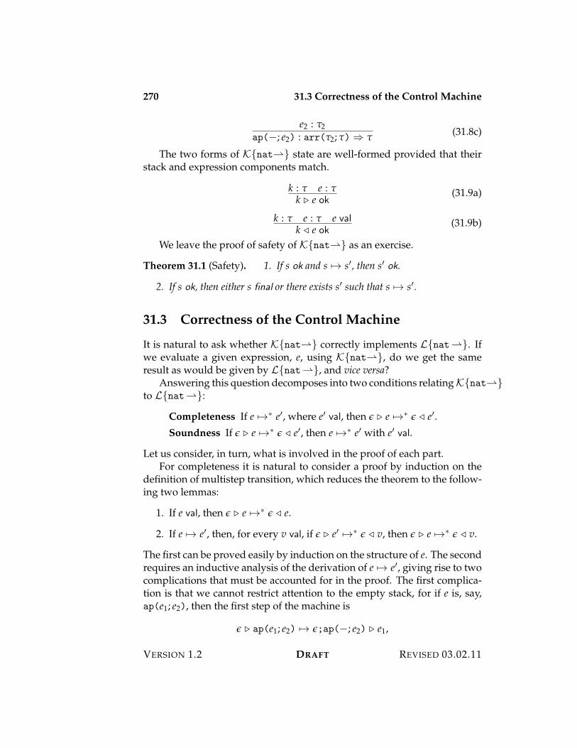
270 31.3 Correctness of the Control Machine
e2 : "2ap($; e2) : arr("2; ") ; " (31.8c)
The two forms of K{nat"} state are well-formed provided that theirstack and expression components match.
k : " e : "k $ e ok
(31.9a)
k : " e : " e valk # e ok
(31.9b)
We leave the proof of safety of K{nat"} as an exercise.
Theorem 31.1 (Safety). 1. If s ok and s 53 s%, then s% ok.
2. If s ok, then either s final or there exists s% such that s 53 s%.
31.3 Correctness of the Control Machine
It is natural to ask whether K{nat"} correctly implements L{nat"}. Ifwe evaluate a given expression, e, using K{nat"}, do we get the sameresult as would be given by L{nat"}, and vice versa?
Answering this question decomposes into two conditions relating K{nat"}to L{nat"}:
Completeness If e 531 e%, where e% val, then % $ e 531 % # e%.Soundness If % $ e 531 % # e%, then e 531 e% with e% val.
Let us consider, in turn, what is involved in the proof of each part.For completeness it is natural to consider a proof by induction on the
definition of multistep transition, which reduces the theorem to the follow-ing two lemmas:
1. If e val, then % $ e 531 % # e.
2. If e 53 e%, then, for every v val, if % $ e% 531 % # v, then % $ e 531 % # v.
The first can be proved easily by induction on the structure of e. The secondrequires an inductive analysis of the derivation of e 53 e%, giving rise to twocomplications that must be accounted for in the proof. The first complica-tion is that we cannot restrict attention to the empty stack, for if e is, say,ap(e1; e2), then the first step of the machine is
% $ ap(e1; e2) 53 %;ap($; e2) $ e1,
VERSION 1.2 DRAFT REVISED 03.02.11
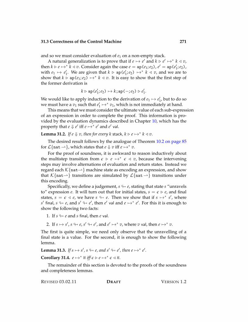
31.3 Correctness of the Control Machine 271
and so we must consider evaluation of e1 on a non-empty stack.A natural generalization is to prove that if e 53 e% and k $ e% 531 k # v,
then k $ e 531 k # v. Consider again the case e = ap(e1; e2), e% = ap(e%1; e2),with e1 53 e%1. We are given that k $ ap(e%1; e2) 531 k # v, and we are toshow that k $ ap(e1; e2) 531 k # v. It is easy to show that the first step ofthe former derivation is
k $ ap(e%1; e2) 53 k;ap($; e2) $ e%1.
We would like to apply induction to the derivation of e1 53 e%1, but to do sowe must have a v1 such that e%1 531 v1, which is not immediately at hand.
This means that we must consider the ultimate value of each sub-expressionof an expression in order to complete the proof. This information is pro-vided by the evaluation dynamics described in Chapter 10, which has theproperty that e " e% iff e 531 e% and e% val.
Lemma 31.2. If e " v, then for every k stack, k $ e 531 k # v.
The desired result follows by the analogue of Theorem 10.2 on page 85for L{nat"}, which states that e " v iff e 531 v.
For the proof of soundness, it is awkward to reason inductively aboutthe multistep transition from % $ e 531 % # v, because the interveningsteps may involve alternations of evaluation and return states. Instead weregard each K{nat"} machine state as encoding an expression, and showthat K{nat"} transitions are simulated by L{nat"} transitions underthis encoding.
Specifically, we define a judgement, s & e, stating that state s “unravelsto” expression e. It will turn out that for initial states, s = % $ e, and finalstates, s = % # e, we have s & e. Then we show that if s 531 s%, wheres% final, s & e, and s% & e%, then e% val and e 531 e%. For this it is enough toshow the following two facts:
1. If s & e and s final, then e val.
2. If s 53 s%, s & e, s% & e%, and e% 531 v, where v val, then e 531 v.
The first is quite simple, we need only observe that the unravelling of afinal state is a value. For the second, it is enough to show the followinglemma.
Lemma 31.3. If s 53 s%, s & e, and s% & e%, then e 531 e%.
Corollary 31.4. e 531 n iff % $ e 531 % # n.
The remainder of this section is devoted to the proofs of the soundnessand completeness lemmas.
REVISED 03.02.11 DRAFT VERSION 1.2
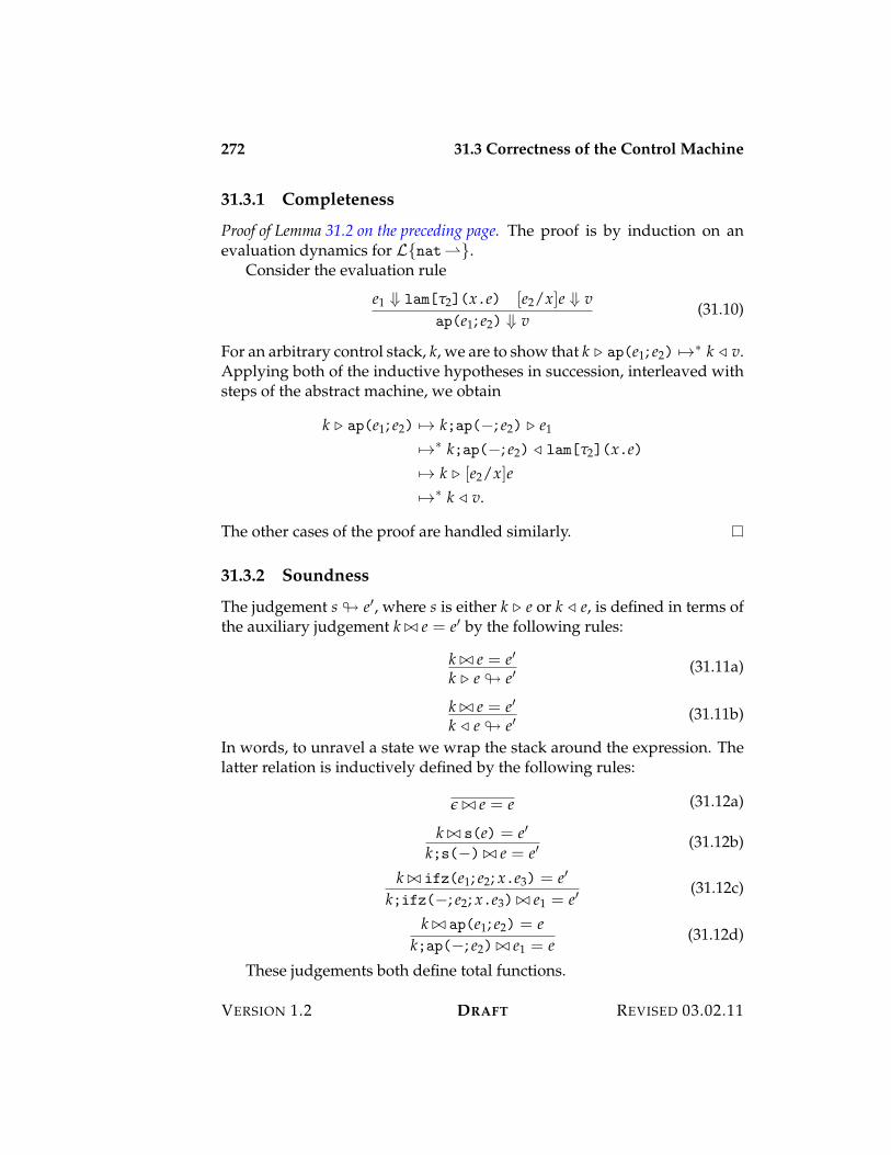
272 31.3 Correctness of the Control Machine
31.3.1 Completeness
Proof of Lemma 31.2 on the preceding page. The proof is by induction on anevaluation dynamics for L{nat"}.
Consider the evaluation rule
e1 " lam["2](x.e) [e2/x]e " vap(e1; e2) " v
(31.10)
For an arbitrary control stack, k, we are to show that k $ ap(e1; e2) 531 k # v.Applying both of the inductive hypotheses in succession, interleaved withsteps of the abstract machine, we obtain
k $ ap(e1; e2) 53 k;ap($; e2) $ e1
531 k;ap($; e2) # lam["2](x.e)53 k $ [e2/x]e531 k # v.
The other cases of the proof are handled similarly.
31.3.2 Soundness
The judgement s & e%, where s is either k $ e or k # e, is defined in terms ofthe auxiliary judgement k $# e = e% by the following rules:
k $# e = e%k $ e & e%
(31.11a)
k $# e = e%k # e & e%
(31.11b)
In words, to unravel a state we wrap the stack around the expression. Thelatter relation is inductively defined by the following rules:
% $# e = e (31.12a)
k $# s(e) = e%k;s($) $# e = e%
(31.12b)
k $# ifz(e1; e2; x.e3) = e%
k;ifz($; e2; x.e3) $# e1 = e%(31.12c)
k $# ap(e1; e2) = ek;ap($; e2) $# e1 = e
(31.12d)
These judgements both define total functions.
VERSION 1.2 DRAFT REVISED 03.02.11
31.4 Exercises 273
Lemma 31.5. The judgement s & e has mode (&, '!), and the judgement k $# e =e% has mode (&, &, '!).
That is, each state unravels to a unique expression, and the result ofwrapping a stack around an expression is uniquely determined. We aretherefore justified in writing k $# e for the unique e% such that k $# e = e%.
The following lemma is crucial. It states that unravelling preserves thetransition relation.
Lemma 31.6. If e 53 e%, k $# e = d, k $# e% = d%, then d 53 d%.
Proof. The proof is by rule induction on the transition e 53 e%. The inductivecases, in which the transition rule has a premise, follow easily by induction.The base cases, in which the transition is an axiom, are proved by an induc-tive analysis of the stack, k.
For an example of an inductive case, suppose that e = ap(e1; e2), e% =ap(e%1; e2), and e1 53 e%1. We have k $# e = d and k $# e% = d%. It follows fromRules (31.12) that k;ap($; e2) $# e1 = d and k;ap($; e2) $# e%1 = d%. So byinduction d 53 d%, as desired.
For an example of a base case, suppose that e = ap(lam["2](x.e); e2)
and e% = [e2/x]e with e 53 e% directly. Assume that k $# e = d and k $# e% = d%;we are to show that d 53 d%. We proceed by an inner induction on thestructure of k. If k = %, the result follows immediately. Consider, say, thestack k = k%;ap($; c2). It follows from Rules (31.12) that k% $# ap(e; c2) = dand k% $# ap(e%; c2) = d%. But by the SOS rules ap(e; c2) 53 ap(e%; c2), so bythe inner inductive hypothesis we have d 53 d%, as desired.
We are now in a position to complete the proof of Lemma 31.3 on page 271.
Proof of Lemma 31.3 on page 271. The proof is by case analysis on the transi-tions of K{nat"}. In each case after unravelling the transition will corre-spond to zero or one transitions of L{nat"}.
Suppose that s = k $ s(e) and s% = k;s($) $ e. Note that k $# s(e) = e%iff k;s($) $# e = e%, from which the result follows immediately.
Suppose that s = k;ap(lam["](x.e1);$) # e2 and s% = k $ [e2/x]e1.Let e% be such that k;ap(lam["](x.e1);$) $# e2 = e% and let e%% be such thatk $# [e2/x]e1 = e%%. Observe that k $# ap(lam["](x.e1); e2) = e%. The resultfollows from Lemma 31.6.
31.4 Exercises
REVISED 03.02.11 DRAFT VERSION 1.2

274 31.4 Exercises
VERSION 1.2 DRAFT REVISED 03.02.11
Chapter 32
Exceptions
Exceptions effect a non-local transfer of control from the point at which theexception is raised to an enclosing handler for that exception. This transferinterrupts the normal flow of control in a program in response to unusualconditions. For example, exceptions can be used to signal an error condi-tion, or to indicate the need for special handling in certain circumstancesthat arise only rarely. To be sure, one could use explicit conditionals tocheck for and process errors or unusual conditions, but using exceptionsis often more convenient, particularly since the transfer to the handler isdirect and immediate, rather than indirect via a series of explicit checks.
32.1 Failures
A failure is a control mechanism that permits a computation to refuse to re-turn a value to the point of its evaluation. Failure can be detected by catch-ing it, diverting evaluation to another expression, called a handler. Failurecan be turned into success, provided that the handler does not itself fail.
The following grammar defines the syntax of failures:
Expr e ::= fail fail failurecatch(e1; e2) catch e1 ow e2 handler
The expression fail aborts the current evaluation, and the expression catch(e1; e2)
handles any failure in e1 by evaluating e2 instead.The statics of failures is straightforward:
! ) fail : "(32.1a)
276 32.1 Failures
! ) e1 : " ! ) e2 : "! ) catch(e1; e2) : "
(32.1b)
A failure can have any type, because it never returns. The two expressionsin a catch expression must have the same type, since either might deter-mine the value of that expression.
The dynamics of failures may be given using stack unwinding. Evalua-tion of a catch installs a handler on the control stack. Evaluation of a fail
unwinds the control stack by popping frames until it reaches the nearestenclosing handler, to which control is passed. The handler is evaluated inthe context of the surrounding control stack, so that failures within it prop-agate further up the stack.
Stack unwinding can be defined directly using structural dynamics, butwe prefer to make use of the stack machine defined in Chapter 31. In ad-dition to states of the form k $ e, which evaluates the expression e on thestack k, and k # e, which passes the value e to the stack k, we make use ofan additional form of state, k ' , which passes a failure up the stack to thenearest enclosing handler.
The set of frames defined in Chapter 31 is extended with the additonalform catch($; e2). The transition rules given in Chapter 31 are extendedwith the following additional rules:
k $ fail 53 k '(32.2a)
k $ catch(e1; e2) 53 k;catch($; e2) $ e1(32.2b)
k;catch($; e2) # v 53 k # v(32.2c)
k;catch($; e2) ' 53 k $ e2(32.2d)
( f ,= catch($; e2))
k; f ' 53 k ' (32.2e)
Evaluating fail propagates a failure up the stack. Evaluating catch(e1; e2)
consists of pushing the handler onto the control stack and evaluating e1.If a value is propagated to the handler, the handler is removed and thevalue continues to propagate upwards. If a failure is propagated to thehandler, the stored expression is evaluated with the handler removed fromthe control stack. All other frames propagate failures.
VERSION 1.2 DRAFT REVISED 03.02.11
32.2 Exceptions 277
The definition of initial state remains the same as for K{nat"}, but wechange the definition of final state to include these two forms:
e val% # e final (32.3a)
% ' final(32.3b)
The first of these is as before, corresponding to a normal result with thespecified value. The second is new, corresponding to an uncaught excep-tion propagating through the entire program.
It is a straightforward exercise the extend the definition of stack typ-ing given in Chapter 31 to account for the new forms of frame. Using this,safety can be proved by standard means. Note, however, that the meaningof the progress theorem is now significantly different: a well-typed pro-gram does not get stuck, but it may well result in an uncaught failure!
Theorem 32.1 (Safety). 1. If s ok and s 53 s%, then s% ok.
2. If s ok, then either s final or there exists s% such that s 53 s%.
32.2 Exceptions
Failures are simplistic in that they do not distinguish different causes, andhence do not permit handlers to react differently to different circumstances.An exception is a generalization of a failure that associates a value with thefailure. This value is passed to the handler, allowing it to discriminate be-tween various forms of failures, and to pass data appropriate to that formof failure. The type of values associated with exceptions is discussed inSection 32.3 on the following page. For now, we simply assume that thereis some type, "exn, of values associated with a failure.
The syntax of exceptions is given by the following grammar:
Expr e ::= raise["](e) raise(e) exceptionhandle(e1; x.e2) handle e1 ow x ; e2 handler
The argument to raise is evaluated to determine the value passed to thehandler. The expression handle(e1; x.e2) binds a variable, x, in the han-dler, e2, to which the associated value of the exception is bound, should anexception be raised during the execution of e1.
REVISED 03.02.11 DRAFT VERSION 1.2
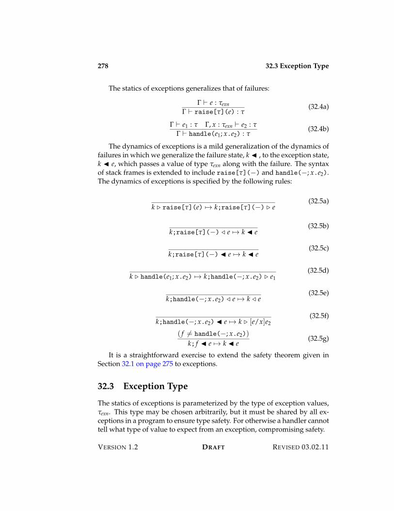
278 32.3 Exception Type
The statics of exceptions generalizes that of failures:
! ) e : "exn! ) raise["](e) : "
(32.4a)
! ) e1 : " !, x : "exn ) e2 : "! ) handle(e1; x.e2) : "
(32.4b)
The dynamics of exceptions is a mild generalization of the dynamics offailures in which we generalize the failure state, k ' , to the exception state,k ' e, which passes a value of type "exn along with the failure. The syntaxof stack frames is extended to include raise["]($) and handle($; x.e2).The dynamics of exceptions is specified by the following rules:
k $ raise["](e) 53 k;raise["]($) $ e(32.5a)
k;raise["]($) # e 53 k ' e(32.5b)
k;raise["]($) ' e 53 k ' e(32.5c)
k $ handle(e1; x.e2) 53 k;handle($; x.e2) $ e1(32.5d)
k;handle($; x.e2) # e 53 k # e(32.5e)
k;handle($; x.e2) ' e 53 k $ [e/x]e2(32.5f)
( f ,= handle($; x.e2))
k; f ' e 53 k ' e(32.5g)
It is a straightforward exercise to extend the safety theorem given inSection 32.1 on page 275 to exceptions.
32.3 Exception Type
The statics of exceptions is parameterized by the type of exception values,"exn. This type may be chosen arbitrarily, but it must be shared by all ex-ceptions in a program to ensure type safety. For otherwise a handler cannottell what type of value to expect from an exception, compromising safety.
VERSION 1.2 DRAFT REVISED 03.02.11
32.3 Exception Type 279
But how do we choose the type of exceptions? A very naıve choicewould be to take "exn to be the type str, so that, for example, one maywrite
raise "Division by zero error."
to signal the obvious arithmetic fault. This is fine as far as it goes, but ahandler for such an exception would have to interpret the string if it is todistinguish one exception from another!
Motivated by this, we might choose "exn to be nat, which amounts tosaying that exceptional conditions are coded as natural numbers.1 Thisdoes allow the handler to distinguish one source of failure from another,but makes no provision for associating data with the failure. Moreover, itforces the programmer to impose a single, global convention for indexingthe causes of failure, compromising modular development and evolution.
The first concern—how to associate data specific to the type of failure—can be addressed by taking "exn to be a labelled sum type whose classes arethe forms of failure, and whose associated types determine the form of thedata attached to the exception. For example, the type "exn might have theform
"exn = [div : unit, fnf : string, . . .].
The class div might represent an arithmetic fault, with no associated data,and the class fnf might represent a “file not found” error, with associateddata being the name of the file.
Using a sum type for "exn makes it easy for the handler to discriminateon the source of the failure, and to recover the associated data without fearof a type safety violation. For example, we might write
try e1 ow x ;match x {
div ?@ ; ediv| fnf s ; efnf }
to handle the exceptions specified by the sum type given in the precedingparagraph.
The problem with choosing a sum type for "exn is that it imposes a staticclassification of the sources of failure in a program. There must be one, glob-ally agreed-upon type that classifies all possible forms of failure, and spec-ifies their associated data. Using sums in this manner impedes modular
1In Unix these are called errno’s, for error numbers.
REVISED 03.02.11 DRAFT VERSION 1.2
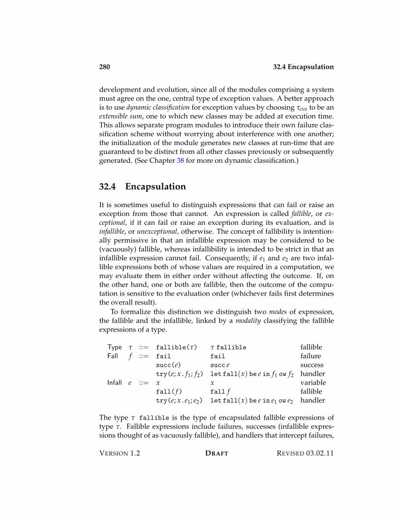
280 32.4 Encapsulation
development and evolution, since all of the modules comprising a systemmust agree on the one, central type of exception values. A better approachis to use dynamic classification for exception values by choosing "exn to be anextensible sum, one to which new classes may be added at execution time.This allows separate program modules to introduce their own failure clas-sification scheme without worrying about interference with one another;the initialization of the module generates new classes at run-time that areguaranteed to be distinct from all other classes previously or subsequentlygenerated. (See Chapter 38 for more on dynamic classification.)
32.4 Encapsulation
It is sometimes useful to distinguish expressions that can fail or raise anexception from those that cannot. An expression is called fallible, or ex-ceptional, if it can fail or raise an exception during its evaluation, and isinfallible, or unexceptional, otherwise. The concept of fallibility is intention-ally permissive in that an infallible expression may be considered to be(vacuously) fallible, whereas infallibility is intended to be strict in that aninfallible expression cannot fail. Consequently, if e1 and e2 are two infal-lible expressions both of whose values are required in a computation, wemay evaluate them in either order without affecting the outcome. If, onthe other hand, one or both are fallible, then the outcome of the compu-tation is sensitive to the evaluation order (whichever fails first determinesthe overall result).
To formalize this distinction we distinguish two modes of expression,the fallible and the infallible, linked by a modality classifying the fallibleexpressions of a type.
Type " ::= fallible(") " fallible fallibleFall f ::= fail fail failure
succ(e) succ e successtry(e; x. f1; f2) let fall(x) be e in f1 ow f2 handler
Infall e ::= x x variablefall( f) fall f fallibletry(e; x.e1; e2) let fall(x) be e in e1 ow e2 handler
The type " fallible is the type of encapsulated fallible expressions oftype ". Fallible expressions include failures, successes (infallible expres-sions thought of as vacuously fallible), and handlers that intercept failures,
VERSION 1.2 DRAFT REVISED 03.02.11
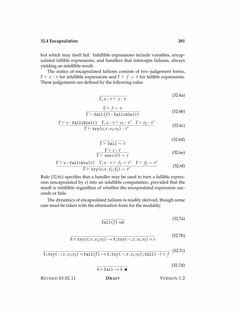
32.4 Encapsulation 281
but which may itself fail. Infallible expressions include variables, encap-sulated fallible expressions, and handlers that intercepts failures, alwaysyielding an infallible result.
The statics of encapsulated failures consists of two judgement forms,! ) e : " for infallible expressions and ! ) f I " for fallible expressions.These judgements are defined by the following rules:
!, x : " ) x : "(32.6a)
! ) f I "
! ) fall( f) : fallible(")(32.6b)
! ) e : fallible(") !, x : " ) e1 : "% ! ) e2 : "%
! ) try(e; x.e1; e2) : "% (32.6c)
! ) fail I "(32.6d)
! ) e : "! ) succ(e) I "
(32.6e)
! ) e : fallible(") !, x : " ) f1 I "% ! ) f2 I "%
! ) try(e; x. f1; f2) I "% (32.6f)
Rule (32.6c) specifies that a handler may be used to turn a fallible expres-sion (encapsulated by e) into an infallible computation, provided that theresult is infallible regardless of whether the encapsulated expression suc-ceeds or fails.
The dynamics of encapsulated failures is readily derived, though somecare must be taken with the elimination form for the modality.
fall( f) val(32.7a)
k $ try(e; x.e1; e2) 53 k;try($; x.e1; e2) $ e(32.7b)
k;try($; x.e1; e2) # fall( f) 53 k;try($; x.e1; e2);fall($) $ f(32.7c)
k $ fail 53 k '(32.7d)
REVISED 03.02.11 DRAFT VERSION 1.2
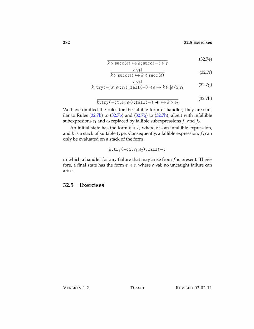
282 32.5 Exercises
k $ succ(e) 53 k;succ($) $ e(32.7e)
e valk $ succ(e) 53 k # succ(e) (32.7f)
e valk;try($; x.e1; e2);fall($) # e 53 k $ [e/x]e1
(32.7g)
k;try($; x.e1; e2);fall($) ' 53 k $ e2(32.7h)
We have omitted the rules for the fallible form of handler; they are sim-ilar to Rules (32.7b) to (32.7b) and (32.7g) to (32.7h), albeit with infalliblesubexpresions e1 and e2 replaced by fallible subexpressions f1 and f2.
An initial state has the form k $ e, where e is an infallible expression,and k is a stack of suitable type. Consequently, a fallible expression, f , canonly be evaluated on a stack of the form
k;try($; x.e1; e2);fall($)
in which a handler for any failure that may arise from f is present. There-fore, a final state has the form % # e, where e val; no uncaught failure canarise.
32.5 Exercises
VERSION 1.2 DRAFT REVISED 03.02.11
Chapter 33
Continuations
The semantics of many control constructs (such as exceptions and co-routines)can be expressed in terms of reified control stacks, a representation of a con-trol stack as an ordinary value. This is achieved by allowing a stack to bepassed as a value within a program and to be restored at a later point, evenif control has long since returned past the point of reification. Reified con-trol stacks of this kind are called continuations, where the qualification “firstclass” stresses that they are ordinary values with an indefinite lifetime thatcan be passed and returned at will in a computation. continuations never“expire”, and it is always sensible to reinstate a continuation without com-promising safety. Thus continuations support unlimited “time travel” —we can go back to a previous point in the computation and then return tosome point in its future, at will.
Why are continuations useful? Fundamentally, they are representationsof the control state of a computation at a given point in time. Using con-tinuations we can “checkpoint” the control state of a program, save it in adata structure, and return to it later. In fact this is precisely what is neces-sary to implement threads (concurrently executing programs) — the threadscheduler must be able to checkpoint a program and save it for later exe-cution, perhaps after a pending event occurs or another thread yields theprocessor.
33.1 Informal Overview
We will extend L{3} with the type cont(") of continuations acceptingvalues of type ". The introduction form for cont(") is letcc["](x.e),which binds the current continuation (that is, the current control stack) to the
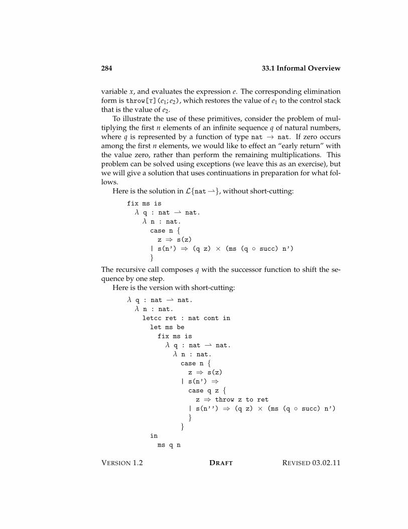
284 33.1 Informal Overview
variable x, and evaluates the expression e. The corresponding eliminationform is throw["](e1; e2), which restores the value of e1 to the control stackthat is the value of e2.
To illustrate the use of these primitives, consider the problem of mul-tiplying the first n elements of an infinite sequence q of natural numbers,where q is represented by a function of type nat 3 nat. If zero occursamong the first n elements, we would like to effect an “early return” withthe value zero, rather than perform the remaining multiplications. Thisproblem can be solved using exceptions (we leave this as an exercise), butwe will give a solution that uses continuations in preparation for what fol-lows.
Here is the solution in L{nat"}, without short-cutting:
fix ms is
! q : nat " nat.
! n : nat.
case n {z ; s(z)
| s(n’) ; (q z) < (ms (q 8 succ) n’)
}The recursive call composes q with the successor function to shift the se-quence by one step.
Here is the version with short-cutting:
! q : nat " nat.
! n : nat.
letcc ret : nat cont in
let ms be
fix ms is
! q : nat " nat.
! n : nat.
case n {z ; s(z)
| s(n’) ;case q z {z ; throw z to ret
| s(n’’) ; (q z) < (ms (q 8 succ) n’)
}}
in
ms q n
VERSION 1.2 DRAFT REVISED 03.02.11
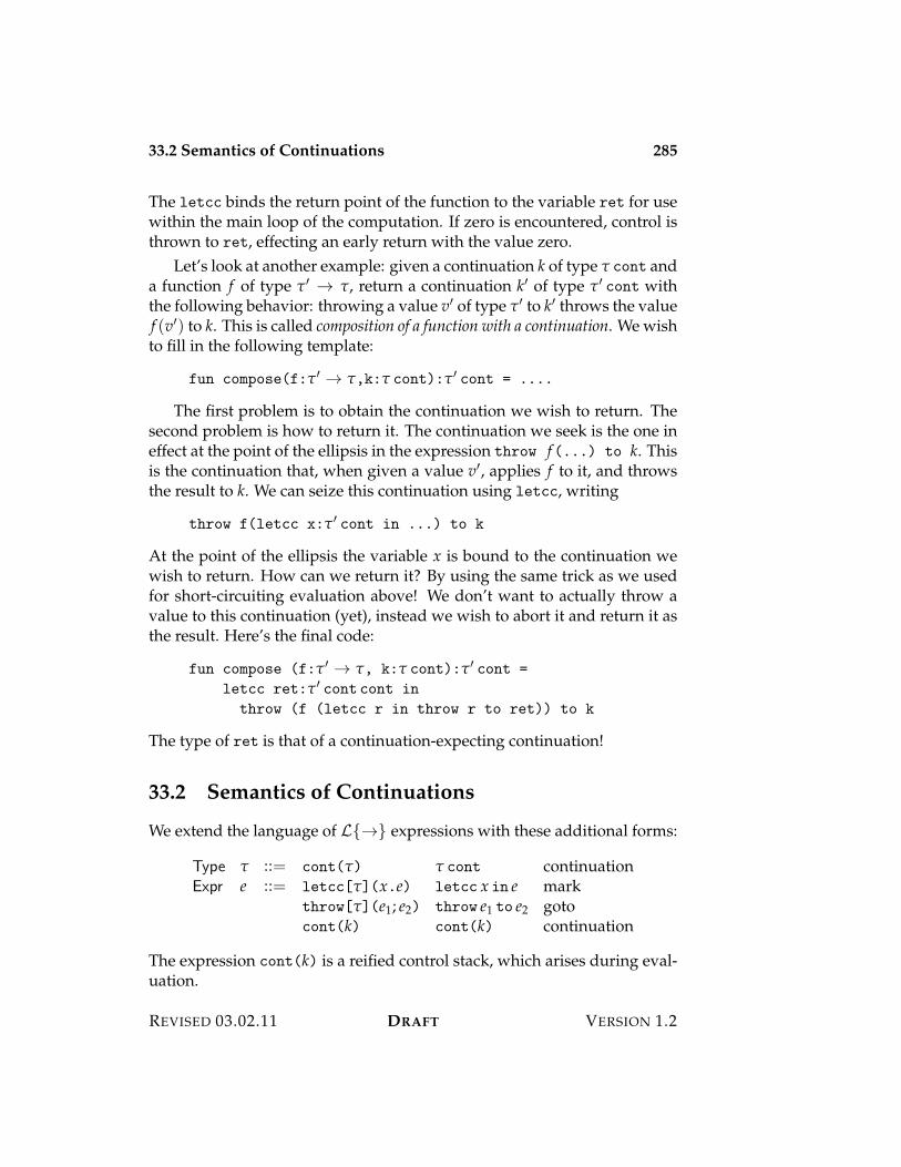
33.2 Semantics of Continuations 285
The letcc binds the return point of the function to the variable ret for usewithin the main loop of the computation. If zero is encountered, control isthrown to ret, effecting an early return with the value zero.
Let’s look at another example: given a continuation k of type " cont anda function f of type "% 3 ", return a continuation k% of type "% cont withthe following behavior: throwing a value v% of type "% to k% throws the valuef (v%) to k. This is called composition of a function with a continuation. We wishto fill in the following template:
fun compose(f:"% 3 ",k:" cont):"% cont = ....
The first problem is to obtain the continuation we wish to return. Thesecond problem is how to return it. The continuation we seek is the one ineffect at the point of the ellipsis in the expression throw f(...) to k. Thisis the continuation that, when given a value v%, applies f to it, and throwsthe result to k. We can seize this continuation using letcc, writing
throw f(letcc x:"% cont in ...) to k
At the point of the ellipsis the variable x is bound to the continuation wewish to return. How can we return it? By using the same trick as we usedfor short-circuiting evaluation above! We don’t want to actually throw avalue to this continuation (yet), instead we wish to abort it and return it asthe result. Here’s the final code:
fun compose (f:"% 3 ", k:" cont):"% cont =
letcc ret:"% cont cont in
throw (f (letcc r in throw r to ret)) to k
The type of ret is that of a continuation-expecting continuation!
33.2 Semantics of Continuations
We extend the language of L{3} expressions with these additional forms:
Type " ::= cont(") " cont continuationExpr e ::= letcc["](x.e) letcc x in e mark
throw["](e1; e2) throw e1 to e2 gotocont(k) cont(k) continuation
The expression cont(k) is a reified control stack, which arises during eval-uation.
REVISED 03.02.11 DRAFT VERSION 1.2
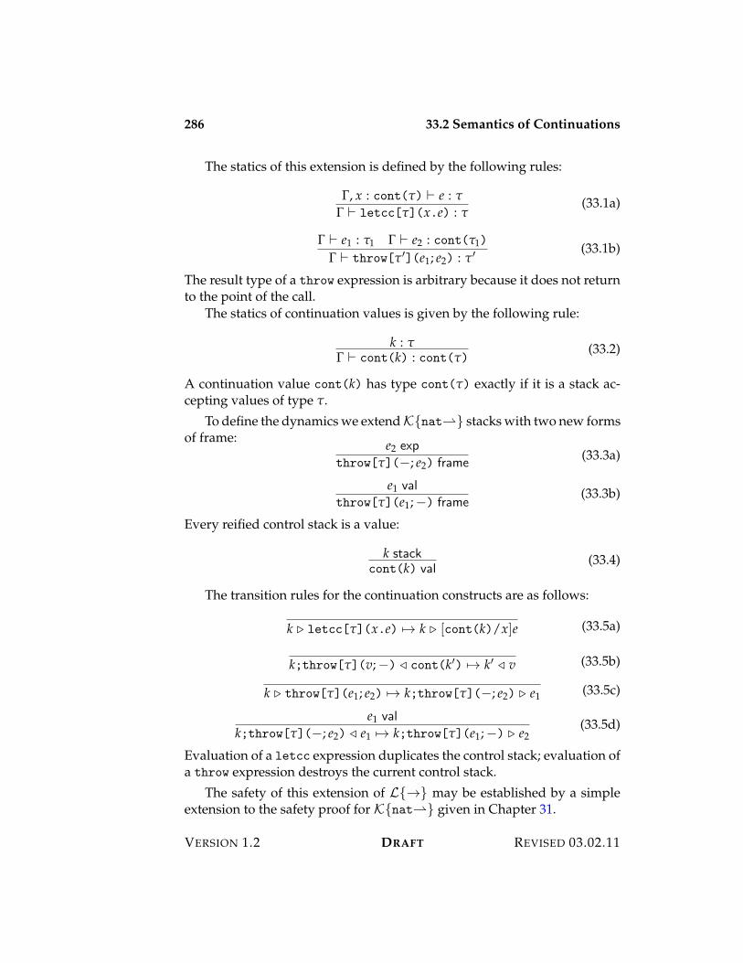
286 33.2 Semantics of Continuations
The statics of this extension is defined by the following rules:
!, x : cont(") ) e : "! ) letcc["](x.e) : "
(33.1a)
! ) e1 : "1 ! ) e2 : cont("1)
! ) throw["%](e1; e2) : "% (33.1b)
The result type of a throw expression is arbitrary because it does not returnto the point of the call.
The statics of continuation values is given by the following rule:
k : "! ) cont(k) : cont(")
(33.2)
A continuation value cont(k) has type cont(") exactly if it is a stack ac-cepting values of type ".
To define the dynamics we extend K{nat"} stacks with two new formsof frame: e2 exp
throw["]($; e2) frame(33.3a)
e1 valthrow["](e1;$) frame
(33.3b)
Every reified control stack is a value:
k stackcont(k) val
(33.4)
The transition rules for the continuation constructs are as follows:
k $ letcc["](x.e) 53 k $ [cont(k)/x]e (33.5a)
k;throw["](v;$) # cont(k%) 53 k% # v (33.5b)
k $ throw["](e1; e2) 53 k;throw["]($; e2) $ e1 (33.5c)
e1 valk;throw["]($; e2) # e1 53 k;throw["](e1;$) $ e2
(33.5d)
Evaluation of a letcc expression duplicates the control stack; evaluation ofa throw expression destroys the current control stack.
The safety of this extension of L{3} may be established by a simpleextension to the safety proof for K{nat"} given in Chapter 31.
VERSION 1.2 DRAFT REVISED 03.02.11
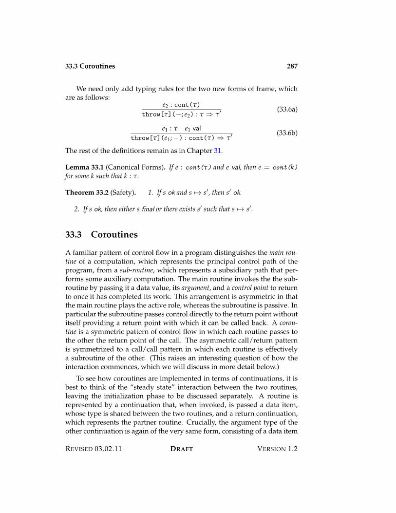
33.3 Coroutines 287
We need only add typing rules for the two new forms of frame, whichare as follows:
e2 : cont(")
throw["]($; e2) : " ; "% (33.6a)
e1 : " e1 val
throw["](e1;$) : cont(") ; "% (33.6b)
The rest of the definitions remain as in Chapter 31.
Lemma 33.1 (Canonical Forms). If e : cont(") and e val, then e = cont(k)for some k such that k : ".
Theorem 33.2 (Safety). 1. If s ok and s 53 s%, then s% ok.
2. If s ok, then either s final or there exists s% such that s 53 s%.
33.3 Coroutines
A familiar pattern of control flow in a program distinguishes the main rou-tine of a computation, which represents the principal control path of theprogram, from a sub-routine, which represents a subsidiary path that per-forms some auxiliary computation. The main routine invokes the the sub-routine by passing it a data value, its argument, and a control point to returnto once it has completed its work. This arrangement is asymmetric in thatthe main routine plays the active role, whereas the subroutine is passive. Inparticular the subroutine passes control directly to the return point withoutitself providing a return point with which it can be called back. A corou-tine is a symmetric pattern of control flow in which each routine passes tothe other the return point of the call. The asymmetric call/return patternis symmetrized to a call/call pattern in which each routine is effectivelya subroutine of the other. (This raises an interesting question of how theinteraction commences, which we will discuss in more detail below.)
To see how coroutines are implemented in terms of continuations, it isbest to think of the “steady state” interaction between the two routines,leaving the initialization phase to be discussed separately. A routine isrepresented by a continuation that, when invoked, is passed a data item,whose type is shared between the two routines, and a return continuation,which represents the partner routine. Crucially, the argument type of theother continuation is again of the very same form, consisting of a data item
REVISED 03.02.11 DRAFT VERSION 1.2
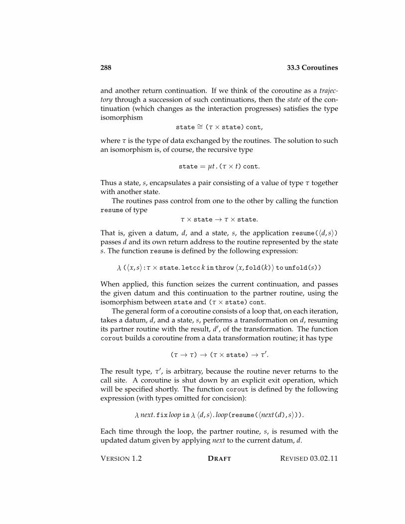
288 33.3 Coroutines
and another return continuation. If we think of the coroutine as a trajec-tory through a succession of such continuations, then the state of the con-tinuation (which changes as the interaction progresses) satisfies the typeisomorphism
state I= (" < state) cont,
where " is the type of data exchanged by the routines. The solution to suchan isomorphism is, of course, the recursive type
state = µt.(" < t) cont.
Thus a state, s, encapsulates a pair consisting of a value of type " togetherwith another state.
The routines pass control from one to the other by calling the functionresume of type
" < state 3 " < state.
That is, given a datum, d, and a state, s, the application resume(?d, s@)passes d and its own return address to the routine represented by the states. The function resume is defined by the following expression:
! (?x, s@:" < state. letcc k in throw ?x, fold(k)@ to unfold(s))
When applied, this function seizes the current continuation, and passesthe given datum and this continuation to the partner routine, using theisomorphism between state and (" < state) cont.
The general form of a coroutine consists of a loop that, on each iteration,takes a datum, d, and a state, s, performs a transformation on d, resumingits partner routine with the result, d%, of the transformation. The functioncorout builds a coroutine from a data transformation routine; it has type
(" 3 ") 3 (" < state) 3 "%.
The result type, "%, is arbitrary, because the routine never returns to thecall site. A coroutine is shut down by an explicit exit operation, whichwill be specified shortly. The function corout is defined by the followingexpression (with types omitted for concision):
! next. fix loop is! ?d, s@. loop(resume(?next(d), s@)).
Each time through the loop, the partner routine, s, is resumed with theupdated datum given by applying next to the current datum, d.
VERSION 1.2 DRAFT REVISED 03.02.11
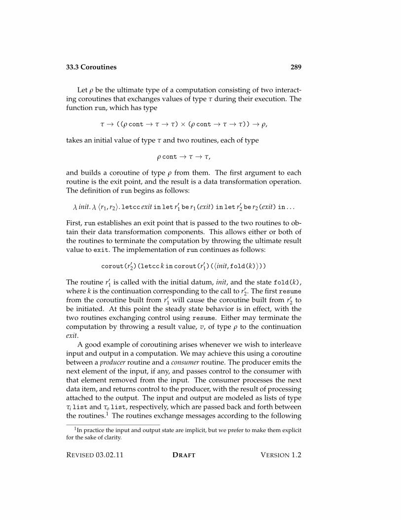
33.3 Coroutines 289
Let , be the ultimate type of a computation consisting of two interact-ing coroutines that exchanges values of type " during their execution. Thefunction run, which has type
" 3 ((, cont 3 " 3 ")< (, cont 3 " 3 ")) 3 ,,
takes an initial value of type " and two routines, each of type
, cont 3 " 3 ",
and builds a coroutine of type , from them. The first argument to eachroutine is the exit point, and the result is a data transformation operation.The definition of run begins as follows:
! init. ! ?r1, r2@. letcc exit in let r%1 be r1(exit) in let r%2 be r2(exit) in . . .
First, run establishes an exit point that is passed to the two routines to ob-tain their data transformation components. This allows either or both ofthe routines to terminate the computation by throwing the ultimate resultvalue to exit. The implementation of run continues as follows:
corout(r%2)(letcc k in corout(r%1)(?init, fold(k)@))
The routine r%1 is called with the initial datum, init, and the state fold(k),where k is the continuation corresponding to the call to r%2. The first resumefrom the coroutine built from r%1 will cause the coroutine built from r%2 tobe initiated. At this point the steady state behavior is in effect, with thetwo routines exchanging control using resume. Either may terminate thecomputation by throwing a result value, v, of type , to the continuationexit.
A good example of coroutining arises whenever we wish to interleaveinput and output in a computation. We may achieve this using a coroutinebetween a producer routine and a consumer routine. The producer emits thenext element of the input, if any, and passes control to the consumer withthat element removed from the input. The consumer processes the nextdata item, and returns control to the producer, with the result of processingattached to the output. The input and output are modeled as lists of type"i list and "o list, respectively, which are passed back and forth betweenthe routines.1 The routines exchange messages according to the following
1In practice the input and output state are implicit, but we prefer to make them explicitfor the sake of clarity.
REVISED 03.02.11 DRAFT VERSION 1.2
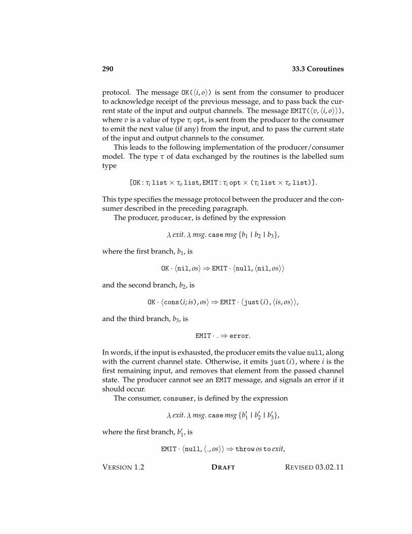
290 33.3 Coroutines
protocol. The message OK(?i, o@) is sent from the consumer to producerto acknowledge receipt of the previous message, and to pass back the cur-rent state of the input and output channels. The message EMIT(?v, ?i, o@@),where v is a value of type "i opt, is sent from the producer to the consumerto emit the next value (if any) from the input, and to pass the current stateof the input and output channels to the consumer.
This leads to the following implementation of the producer/consumermodel. The type " of data exchanged by the routines is the labelled sumtype
[OK : "i list< "o list, EMIT : "i opt< ("i list< "o list)].
This type specifies the message protocol between the producer and the con-sumer described in the preceding paragraph.
The producer, producer, is defined by the expression
! exit. ! msg. casemsg {b1 | b2 | b3},
where the first branch, b1, is
OK · ?nil, os@ ; EMIT · ?null, ?nil, os@@
and the second branch, b2, is
OK · ?cons(i; is), os@ ; EMIT · ?just(i), ?is, os@@,
and the third branch, b3, is
EMIT · ; error.
In words, if the input is exhausted, the producer emits the value null, alongwith the current channel state. Otherwise, it emits just(i), where i is thefirst remaining input, and removes that element from the passed channelstate. The producer cannot see an EMIT message, and signals an error if itshould occur.
The consumer, consumer, is defined by the expression
! exit. ! msg. casemsg {b%1 | b%2 | b%3},
where the first branch, b%1, is
EMIT · ?null, ? , os@@ ; throw os to exit,
VERSION 1.2 DRAFT REVISED 03.02.11

33.4 Exercises 291
the second branch, b%2, is
EMIT · ?just(i), ?is, os@@ ; OK · ?is, cons( f(i); os)@,
and the third branch, b%3, is
OK · ; error.
The consumer dispatches on the emitted datum. If it is absent, the outputchannel state is passed to exit as the ultimate value of the computation. Ifit is present, the function f (unspecified here) of type "i 3 "o is appliedto transform the input to the output, and the result is added to the outputchannel. If the message OK is received, the consumer signals an error, as theproducer never produces such a message.
The initial datum, init, has the form OK · ?is, os@, where is and os arethe initial input and output channel state, respectively. The computation iscreated by the expression
run(init)(?producer, consumer@),
which sets up the coroutines as described earlier.While it is relatively easy to visualize and implement coroutines involv-
ing only two partners, it is more complex, and less useful, to consider asimilar pattern of control among n 7 2 participants. In such cases it ismore common to structure the interaction as a collection of n routines, eachof which is a coroutine of a central scheduler. When a routine resumes itspartner, it passes control to the scheduler, which determines which routineto execute next, again as a coroutine of itself. When structured as corou-tines of a scheduler, the individual routines are called threads. A threadyields control by resuming its partner, the scheduler, which then determineswhich thread to execute next as a coroutine of itself. This pattern of con-trol is called cooperative multi-threading, since it is based on explicit yields,rather than implicit yields imposed by asynchronous events such as timerinterrupts.
33.4 Exercises
1. Study the short-circuit multiplication example carefully to be sureyou understand why it works!
2. Attempt to solve the problem of composing a continuation with afunction yourself, before reading the solution.
REVISED 03.02.11 DRAFT VERSION 1.2
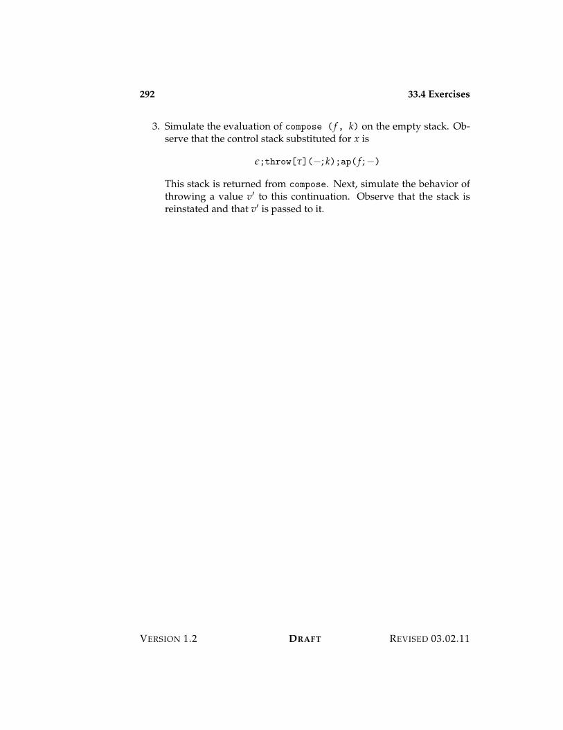
292 33.4 Exercises
3. Simulate the evaluation of compose ( f, k) on the empty stack. Ob-serve that the control stack substituted for x is
%;throw["]($; k);ap( f ;$)
This stack is returned from compose. Next, simulate the behavior ofthrowing a value v% to this continuation. Observe that the stack isreinstated and that v% is passed to it.
VERSION 1.2 DRAFT REVISED 03.02.11
Part XII
Types and Propositions

Chapter 34
Constructive Logic
The correspondence between propositions and types, and the associated cor-respondence between proofs and programs, is the central organizing princi-ple of programming languages. A type specifies a behavior, and a programimplements it. Similarly, a proposition poses a problem, and a proof solvesit. A statics relates a program to the type it implements, and a dynamicsrelates a program to its simplification by an execution step. Similarly, a for-mal logical system relates a proof to the proposition it proves, and proofreduction relates equivalent proofs. The structural rule of substitution un-derlies the decomposition of a program into separate modules. Similarly,the structural rule of transitivity underlies the decomposition of a theoreminto lemmas.
These correspondences are neither accidental nor incidental. The propo-sitions as types principle,1 identifies propositions with types and proofs withprograms. According to this principle, a proposition is the type of its proofs,and a proof is a program of that type. Consequently, every theorem hascomputational content, the its proof viewed as a program, and every pro-gram has mathematical content, the proof that the program represents.
Can every conceivable form of proposition also be construed as a type?Does every type correspond to a proposition? Must every proof have com-putational content? Is every program a proof of a theorem? To answerthese questions would require a book of its own (and still not settle thematter). From a constructive perspective we may say that type theory en-
1The propositions-as-types principle is sometimes called the Curry-Howard Isomorphism.Although it is arguably snappier, this name ignores the essential contributions of ArendHeyting, Nicolaas deBruijn, and Per Martin-Lof to the development of the propositions-as-types principle.
296 34.1 Constructive Semantics
riches logic to incorporate not only types of proofs, but also types for theobjects of study. In this sense logic is a particular mode of use of type the-ory. If we think of type theory as a comprehensive view of mathematics,this implies that, contrary to conventional wisdom, logic is based on math-ematics, rather than mathematics on logic!
In this chapter we introduce the propositions-as-types correspondencefor a particularly simple system of logic, called propositional contructive logic.In Chapter 35 we will extend the correspondence to propositional classicallogic. This will give rise to a computational interpretation of classical proofsthat makes essential use of continuations.
34.1 Constructive Semantics
Constructive logic is concerned with two judgements, ' prop, stating that' expresses a proposition, and ' true, stating that ' is a true proposi-tion. What distinguishes constructive from non-constructive logic is thata proposition is not conceived of as merely a truth value, but instead as aproblem statement whose solution, if it has one, is given by a proof. A propo-sition is said to be true exactly when it has a proof, in keeping with ordinarymathematical practice. There is no other criterion of truth than the existence ofa proof.
This principle has important, possibly surprising, consequences, themost important of which is that we cannot say, in general, that a propo-sition is either true or false. If for a proposition to be true means to havea proof of it, what does it mean for a proposition to be false? It meansthat we have a refutation of it, showing that it cannot be proved. That is, aproposition is false if we can show that the assumption that it is true (has aproof) contradicts known facts. In this sense constructive logic is a logic ofpositive, or affirmative, information — we must have explicit evidence in theform of a proof in order to affirm the truth or falsity of a proposition.
In light of this it should be clear that not every proposition is eithertrue or false. For if ' expresses an unsolved problem, such as the famousP
?= NP problem, then we have neither a proof nor a refutation of it (the
mere absence of a proof not being a refutation). Such a problem is unde-cided, precisely because it is unsolved. Since there will always be unsolvedproblems (there being infinitely many propositions, but only finitely manyproofs at a given point in the evolution of our knowledge), we cannot saythat every proposition is decidable, that is, either true or false.
Having said that, some propositions are decidable, and hence may be
VERSION 1.2 DRAFT REVISED 03.02.11
34.2 Constructive Logic 297
considered to be either true or false. For example, if ' expresses an inequal-ity between natural numbers, then ' is decidable, because we can alwayswork out, for given natural numbers m and n, whether m ( n or m ,( n —we can either prove or refute the given inequality. This argument does notextend to the real numbers. To get an idea of why not, consider the presen-tation of a real number by its decimal expansion. At any finite time we willhave explored only a finite initial segment of the expansion, which is notenough to determine if it is, say, less than 1. For if we have determined theexpansion to be 0.99 . . . 9, we cannot decide at any time, short of infinity,whether or not the number is 1. (This argument is not a proof, because onemay wonder whether there is some other representation of real numbersthat admits such a decision to be made finitely, but it turns out that this isnot the case.)
The constructive attitude is simply to accept the situation as inevitable,and make our peace with that. When faced with a problem we have nochoice but to roll up our sleeves and try to prove it or refute it. There is noguarantee of success! Life’s hard, but we muddle through somehow.
34.2 Constructive Logic
The judgements ' prop and ' true of constructive logic are rarely of interestby themselves, but rather in the context of a hypothetical judgement of theform
'1 true, . . . , 'n true ) ' true.
This judgement expresses that the proposition ' is true (has a proof), underthe assumptions that each of '1, . . . , 'n are also true (have proofs). Of course,when n = 0 this is just the same as the judgement ' true.
The structural properties of the hypothetical judgement, when special-ized to constructive logic, define what we mean by reasoning under hy-potheses:
!, ' true ) ' true (34.1a)
! ) '1 true !, '1 true ) '2 true
! ) '2 true(34.1b)
! ) '2 true
!, '1 true ) '2 true(34.1c)
!, '1 true, '1 true ) '2 true
!, '1 true ) '2 true(34.1d)
REVISED 03.02.11 DRAFT VERSION 1.2
298 34.2 Constructive Logic
!1, '2 true, '1 true, !2 ) ' true
!1, '1 true, '2 true, !2 ) ' true(34.1e)
The last two rules are implicit in that we regard ! as a set of hypotheses, sothat two “copies” are as good as one, and the order of hypotheses does notmatter.
34.2.1 Rules of Provability
The syntax of propositional logic is given by the following grammar:
Prop ' ::= true F truthfalse > falsityand('1; '2) '1 4 '2 conjunctionor('1; '2) '1 G '2 disjunctionimp('1; '2) '1 H '2 implication
The connectives of propositional logic are given meaning by rules that de-termine (a) what constitutes a “direct” proof of a proposition formed froma given connective, and (b) how to exploit the existence of such a proof inan “indirect” proof of another proposition. These are called the introduc-tion and elimination rules for the connective. The principle of conservationof proof states that these rules are inverse to one another — the eliminationrule cannot extract more information (in the form of a proof) than was putinto it by the introduction rule, and the introduction rules can be used to re-construct a proof from the information extracted from it by the eliminationrules.
Truth Our first proposition is trivially true. No information goes intoproving it, and so no information can be obtained from it.
! ) F true (34.2a)
(no elimination rule)(34.2b)
Conjunction Conjunction expresses the truth of both of its conjuncts.
! ) '1 true ! ) '2 true
! ) '1 4 '2 true(34.3a)
! ) '1 4 '2 true
! ) '1 true(34.3b)
VERSION 1.2 DRAFT REVISED 03.02.11
34.2 Constructive Logic 299
! ) '1 4 '2 true
! ) '2 true(34.3c)
Implication Implication states the truth of a proposition under an as-sumption.
!, '1 true ) '2 true
! ) '1 H '2 true(34.4a)
! ) '1 H '2 true ! ) '1 true
! ) '2 true(34.4b)
Falsehood Falsehood expresses the trivially false (refutable) proposition.
(no introduction rule)(34.5a)
! ) > true! ) ' true
(34.5b)
Disjunction Disjunction expresses the truth of either (or both) of twopropositions.
! ) '1 true
! ) '1 G '2 true(34.6a)
! ) '2 true
! ) '1 G '2 true(34.6b)
! ) '1 G '2 true !, '1 true ) ' true !, '2 true ) ' true
! ) ' true(34.6c)
Negation The negation, ¬', of a proposition, ', may be defined as theimplication ' H>. This means that ¬' true if ' true ) > true, whichis to say that the truth of ' is refutable in that we may derive a proof offalsehood from any purported proof of '. Because constructive truth isidentified with the existence of a proof, the implied semantics of negationis rather strong. In particular, a problem, ', is open exactly when we canneither affirm nor refute it. This is in contrast to the classical conception oftruth, which assigns a fixed truth value to each proposition, so that everyproposition is either true or false.
REVISED 03.02.11 DRAFT VERSION 1.2
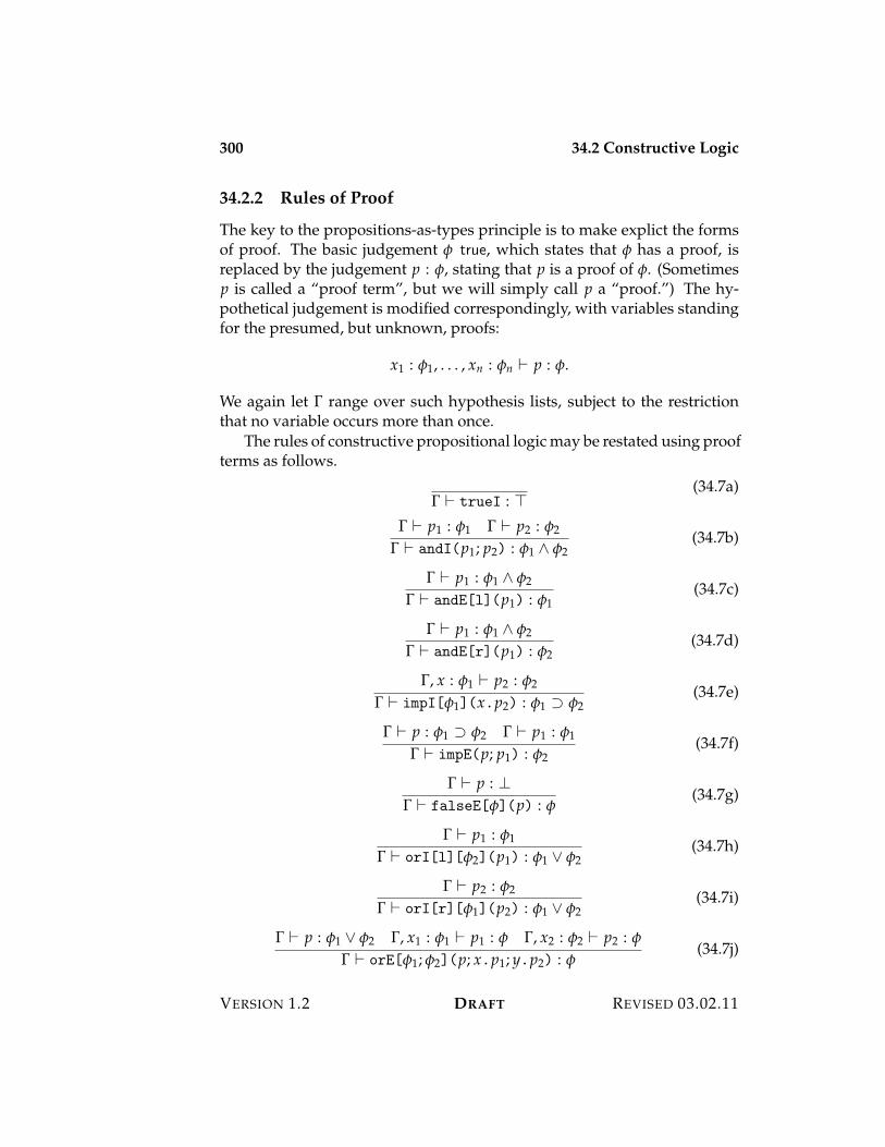
300 34.2 Constructive Logic
34.2.2 Rules of Proof
The key to the propositions-as-types principle is to make explict the formsof proof. The basic judgement ' true, which states that ' has a proof, isreplaced by the judgement p : ', stating that p is a proof of '. (Sometimesp is called a “proof term”, but we will simply call p a “proof.”) The hy-pothetical judgement is modified correspondingly, with variables standingfor the presumed, but unknown, proofs:
x1 : '1, . . . , xn : 'n ) p : '.
We again let ! range over such hypothesis lists, subject to the restrictionthat no variable occurs more than once.
The rules of constructive propositional logic may be restated using proofterms as follows.
! ) trueI : F(34.7a)
! ) p1 : '1 ! ) p2 : '2
! ) andI(p1; p2) : '1 4 '2(34.7b)
! ) p1 : '1 4 '2
! ) andE[l](p1) : '1(34.7c)
! ) p1 : '1 4 '2
! ) andE[r](p1) : '2(34.7d)
!, x : '1 ) p2 : '2
! ) impI['1](x.p2) : '1 H '2(34.7e)
! ) p : '1 H '2 ! ) p1 : '1
! ) impE(p; p1) : '2(34.7f)
! ) p : >! ) falseE['](p) : '
(34.7g)
! ) p1 : '1
! ) orI[l]['2](p1) : '1 G '2(34.7h)
! ) p2 : '2
! ) orI[r]['1](p2) : '1 G '2(34.7i)
! ) p : '1 G '2 !, x1 : '1 ) p1 : ' !, x2 : '2 ) p2 : '
! ) orE['1; '2](p; x.p1; y.p2) : '(34.7j)
VERSION 1.2 DRAFT REVISED 03.02.11
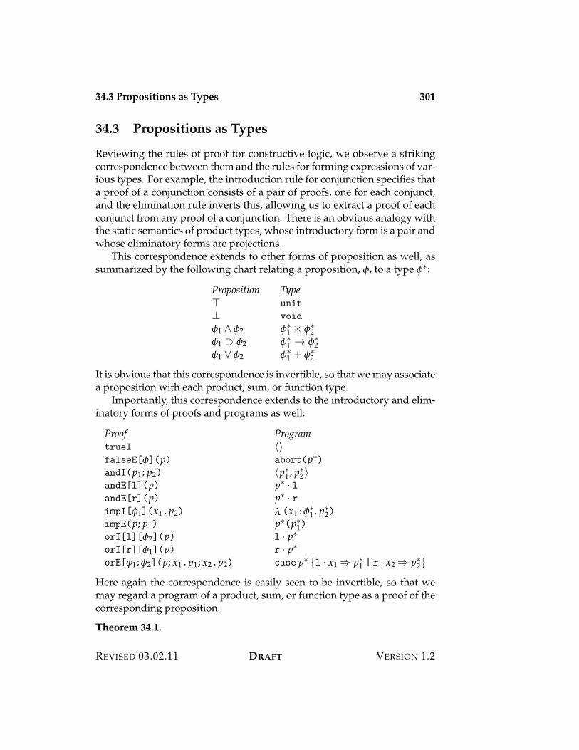
34.3 Propositions as Types 301
34.3 Propositions as Types
Reviewing the rules of proof for constructive logic, we observe a strikingcorrespondence between them and the rules for forming expressions of var-ious types. For example, the introduction rule for conjunction specifies thata proof of a conjunction consists of a pair of proofs, one for each conjunct,and the elimination rule inverts this, allowing us to extract a proof of eachconjunct from any proof of a conjunction. There is an obvious analogy withthe static semantics of product types, whose introductory form is a pair andwhose eliminatory forms are projections.
This correspondence extends to other forms of proposition as well, assummarized by the following chart relating a proposition, ', to a type '1:
Proposition TypeF unit
> void
'1 4 '2 '11 < '1
2'1 H '2 '1
1 3 '12
'1 G '2 '11 + '1
2
It is obvious that this correspondence is invertible, so that we may associatea proposition with each product, sum, or function type.
Importantly, this correspondence extends to the introductory and elim-inatory forms of proofs and programs as well:
Proof ProgramtrueI ?@falseE['](p) abort(p1)andI(p1; p2) ?p11, p12@andE[l](p) p1 · landE[r](p) p1 · rimpI['1](x1.p2) ! (x1:'1
1 . p12)impE(p; p1) p1(p11)orI[l]['2](p) l · p1orI[r]['1](p) r · p1orE['1; '2](p; x1.p1; x2.p2) case p1 {l · x1 ; p11 | r · x2 ; p12}
Here again the correspondence is easily seen to be invertible, so that wemay regard a program of a product, sum, or function type as a proof of thecorresponding proposition.
Theorem 34.1.
REVISED 03.02.11 DRAFT VERSION 1.2
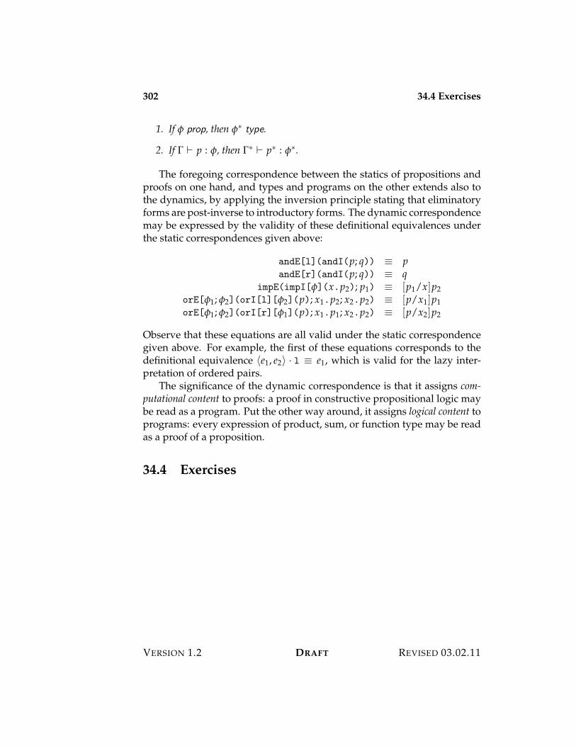
302 34.4 Exercises
1. If ' prop, then '1 type.
2. If ! ) p : ', then !1 ) p1 : '1.
The foregoing correspondence between the statics of propositions andproofs on one hand, and types and programs on the other extends also tothe dynamics, by applying the inversion principle stating that eliminatoryforms are post-inverse to introductory forms. The dynamic correspondencemay be expressed by the validity of these definitional equivalences underthe static correspondences given above:
andE[l](andI(p; q)) 9 pandE[r](andI(p; q)) 9 q
impE(impI['](x.p2); p1) 9 [p1/x]p2orE['1; '2](orI[l]['2](p); x1.p2; x2.p2) 9 [p/x1]p1orE['1; '2](orI[r]['1](p); x1.p1; x2.p2) 9 [p/x2]p2
Observe that these equations are all valid under the static correspondencegiven above. For example, the first of these equations corresponds to thedefinitional equivalence ?e1, e2@ · l 9 e1, which is valid for the lazy inter-pretation of ordered pairs.
The significance of the dynamic correspondence is that it assigns com-putational content to proofs: a proof in constructive propositional logic maybe read as a program. Put the other way around, it assigns logical content toprograms: every expression of product, sum, or function type may be readas a proof of a proposition.
34.4 Exercises
VERSION 1.2 DRAFT REVISED 03.02.11

Chapter 35
Classical Logic
In constructive logic a proposition is true exactly when it has a proof, aderivation of it from axioms and assumptions, and is false exactly whenit has a refutation, a derivation of a contradiction from the assumption thatit is true. Constructive logic is a logic of positive evidence. To affirm ordeny a proposition requires a proof, either of the proposition itself, or ofa contradiction, under the assumption that it has a proof. We are not al-ways in a position to affirm or deny a proposition. An open problem is onefor which we have neither a proof nor a refutation—so that, constructivelyspeaking, it is neither true nor false!
In contrast classical logic (the one we learned in school) is a logic ofperfect information in which every proposition is either true or false. Onemay say that classical logic corresponds to “god’s view” of the world—there are no open problems, rather all propositions are either true or false.Put another way, to assert that every proposition is either true or false isto weaken the notion of truth to encompass all that is not false, dually to theconstructively (and classically) valid interpretation of falsity as all that isnot true. The symmetry between truth and falsity is appealing, but there isa price to pay for this: the meanings of the logical connectives are weakerin the classical case than in the constructive.
A prime example is provided by the law of the excluded middle, the as-sertion that ' G ¬' true is valid for all propositions '. Constructively, thisprinciple is not universally valid, because it would mean that every propo-sition either has a proof or a refutation, which is manifestly not the case.Classically, however, the law of the excluded middle is valid, because everyproposition is either true or false. The discrepancy between the construc-tive and classical interpretations can be attributed to the different meanings
304 35.1 Classical Logic
given to disjunction and negation by the two logics. In particular the classi-cal truth of a disjunction cannot guarantee the constructive truth of one orthe other disjunct. Something other than a constructive proof must be ad-mitted as evidence for a disjunction if the law of the excluded middle is tohold true. And it is precisely for this reason that a classical proof expressesless than does a constructive proof of the same proposition.
Despite this weakness, classical logic admits a computational interpre-tation similar to, but somewhat less expressive than, that of constructivelogic. The dynamics of classical proofs is derived from the complementar-ity of truth and falsity. A computation is initiated by juxtaposing a proofand a refutation—or, in programming terms, an expression and a continua-tion, or control stack. Continuations are essential to the meaning of classicalproofs. In particular, the proof of the law of the excluded middle will beseen to equivocate between proving and refuting a proposition, using con-tinuations to avoid getting caught in a contradiction.
35.1 Classical Logic
In constructive logic a connective is defined by giving its introduction andelimination rules. In classical logic a connective is defined by giving itstruth and falsity conditions. Its truth rules correspond to introduction, andits falsity rules to elimination. The symmetry between truth and falsity isexpressed by the principle of indirect proof. To show that ' true it is enoughto show that ' false entails a contradiction, and, conversely, to show that' false it is enough to show that ' true leads to a contradiction. While thesecond of these is constructively valid, the first is fundamentally classical,expressing the principle of indirect proof.
35.1.1 Provability and Refutability
There are three judgement forms in classical logic:
1. ' true, stating that the proposition ' is provable;
2. ' false, stating that the proposition ' is refutable;
3. #, stating that a contradiction has been derived.
We will consider hypothetical judgements of the form
'1 false, . . . , 'm false (1 true, . . . , (n true ) J,
VERSION 1.2 DRAFT REVISED 03.02.11
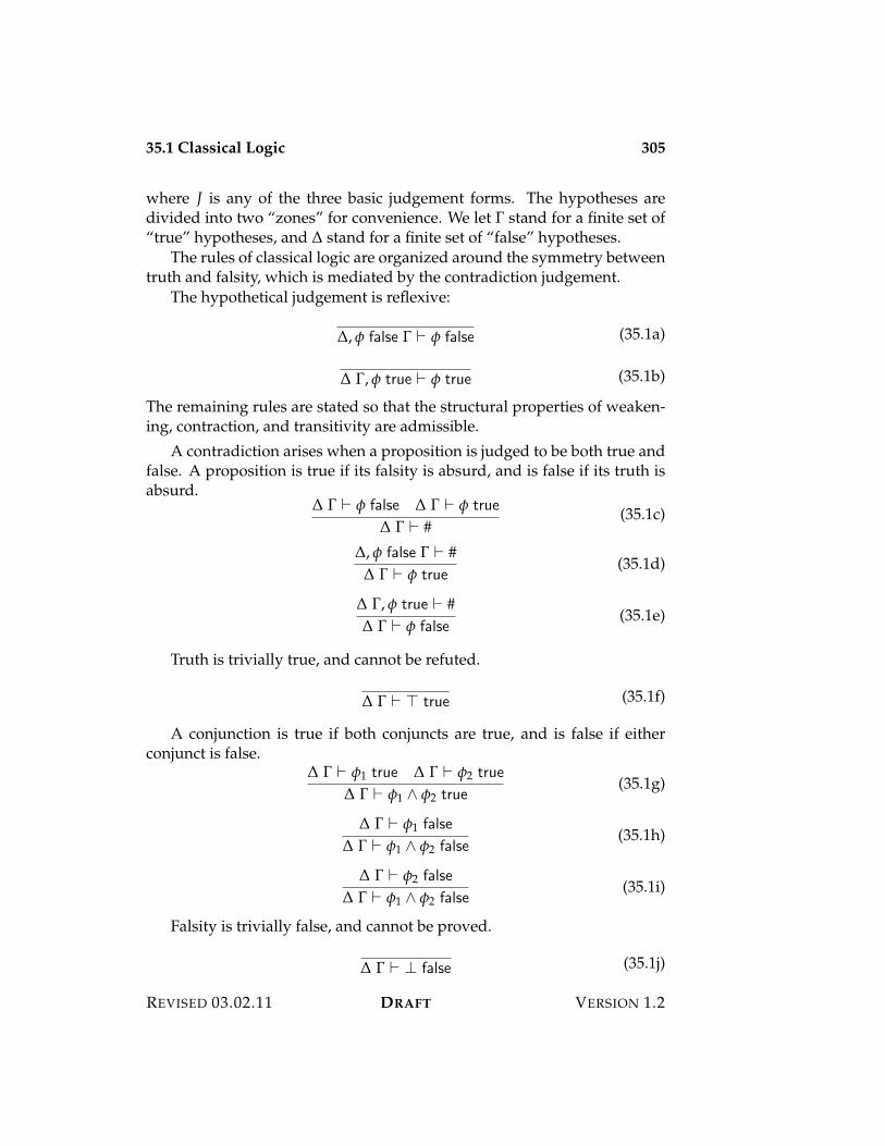
35.1 Classical Logic 305
where J is any of the three basic judgement forms. The hypotheses aredivided into two “zones” for convenience. We let ! stand for a finite set of“true” hypotheses, and " stand for a finite set of “false” hypotheses.
The rules of classical logic are organized around the symmetry betweentruth and falsity, which is mediated by the contradiction judgement.
The hypothetical judgement is reflexive:
", ' false ! ) ' false (35.1a)
" !, ' true ) ' true (35.1b)
The remaining rules are stated so that the structural properties of weaken-ing, contraction, and transitivity are admissible.
A contradiction arises when a proposition is judged to be both true andfalse. A proposition is true if its falsity is absurd, and is false if its truth isabsurd.
" ! ) ' false " ! ) ' true
" ! ) #(35.1c)
", ' false ! ) #" ! ) ' true
(35.1d)
" !, ' true ) #" ! ) ' false
(35.1e)
Truth is trivially true, and cannot be refuted.
" ! ) F true (35.1f)
A conjunction is true if both conjuncts are true, and is false if eitherconjunct is false.
" ! ) '1 true " ! ) '2 true
" ! ) '1 4 '2 true(35.1g)
" ! ) '1 false
" ! ) '1 4 '2 false(35.1h)
" ! ) '2 false
" ! ) '1 4 '2 false(35.1i)
Falsity is trivially false, and cannot be proved.
" ! ) > false (35.1j)
REVISED 03.02.11 DRAFT VERSION 1.2
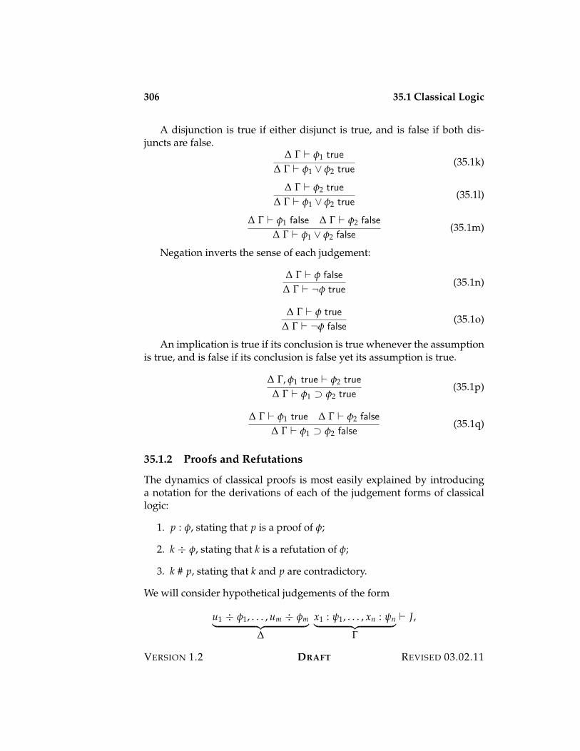
306 35.1 Classical Logic
A disjunction is true if either disjunct is true, and is false if both dis-juncts are false.
" ! ) '1 true
" ! ) '1 G '2 true(35.1k)
" ! ) '2 true
" ! ) '1 G '2 true(35.1l)
" ! ) '1 false " ! ) '2 false
" ! ) '1 G '2 false(35.1m)
Negation inverts the sense of each judgement:
" ! ) ' false
" ! ) ¬' true(35.1n)
" ! ) ' true
" ! ) ¬' false(35.1o)
An implication is true if its conclusion is true whenever the assumptionis true, and is false if its conclusion is false yet its assumption is true.
" !, '1 true ) '2 true
" ! ) '1 H '2 true(35.1p)
" ! ) '1 true " ! ) '2 false
" ! ) '1 H '2 false(35.1q)
35.1.2 Proofs and Refutations
The dynamics of classical proofs is most easily explained by introducinga notation for the derivations of each of the judgement forms of classicallogic:
1. p : ', stating that p is a proof of ';
2. k ÷ ', stating that k is a refutation of ';
3. k # p, stating that k and p are contradictory.
We will consider hypothetical judgements of the form
u1 ÷ '1, . . . , um ÷ 'm! "# $"
x1 : (1, . . . , xn : (n! "# $!
) J,
VERSION 1.2 DRAFT REVISED 03.02.11
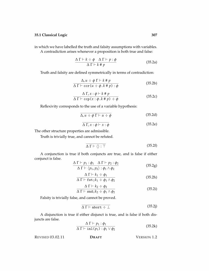
35.1 Classical Logic 307
in which we have labelled the truth and falsity assumptions with variables.A contradiction arises whenever a proposition is both true and false:
" ! ) k ÷ ' " ! ) p : '
" ! ) k # p(35.2a)
Truth and falsity are defined symmetrically in terms of contradiction:
", u ÷ ' ! ) k # p" ! ) ccr(u ÷ '.k # p) : '
(35.2b)
" !, x : ' ) k # p" ! ) ccp(x : '.k # p) ÷ '
(35.2c)
Reflexivity corresponds to the use of a variable hypothesis:
", u ÷ ' ! ) u ÷ ' (35.2d)
" !, x : ' ) x : ' (35.2e)
The other structure properties are admissible.Truth is trivially true, and cannot be refuted.
" ! ) ?@ : F (35.2f)
A conjunction is true if both conjuncts are true, and is false if eitherconjunct is false.
" ! ) p1 : '1 " ! ) p2 : '2
" ! ) ?p1, p2@ : '1 4 '2(35.2g)
" ! ) k1 ÷ '1
" ! ) fst;k1 ÷ '1 4 '2(35.2h)
" ! ) k2 ÷ '2
" ! ) snd;k2 ÷ '1 4 '2(35.2i)
Falsity is trivially false, and cannot be proved.
" ! ) abort ÷ > (35.2j)
A disjunction is true if either disjunct is true, and is false if both dis-juncts are false.
" ! ) p1 : '1
" ! ) inl(p1) : '1 G '2(35.2k)
REVISED 03.02.11 DRAFT VERSION 1.2
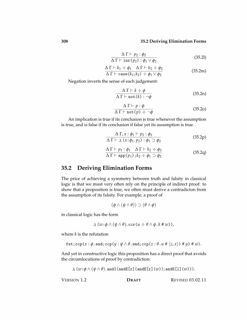
308 35.2 Deriving Elimination Forms
" ! ) p2 : '2
" ! ) inr(p2) : '1 G '2(35.2l)
" ! ) k1 ÷ '1 " ! ) k2 ÷ '2
" ! ) case(k1; k2) ÷ '1 G '2(35.2m)
Negation inverts the sense of each judgement:
" ! ) k ÷ '
" ! ) not(k) : ¬'(35.2n)
" ! ) p : '
" ! ) not(p) ÷ ¬'(35.2o)
An implication is true if its conclusion is true whenever the assumptionis true, and is false if its conclusion if false yet its assumption is true.
" !, x : '1 ) p2 : '2
" ! ) ! (x:'1. p2) : '1 H '2(35.2p)
" ! ) p1 : '1 " ! ) k2 ÷ '2
" ! ) app(p1);k2 ÷ '1 H '2(35.2q)
35.2 Deriving Elimination Forms
The price of achieving a symmetry between truth and falsity in classicallogic is that we must very often rely on the principle of indirect proof: toshow that a proposition is true, we often must derive a contradicton fromthe assumption of its falsity. For example, a proof of
(' 4 (( 4 *)) H (* 4 ')
in classical logic has the form
! (w:' 4 (( 4 *). ccr(u ÷ * 4 '.k # w)),
where k is the refutation
fst;ccp(x : '.snd;ccp(y : ( 4 *.snd;ccp(z : *.u # ?z, x@) # y) # w).
And yet in constructive logic this proposition has a direct proof that avoidsthe circumlocutions of proof by contradiction:
! (w:' 4 (( 4 *). andI(andE[r](andE[r](w)); andE[l](w))).
VERSION 1.2 DRAFT REVISED 03.02.11
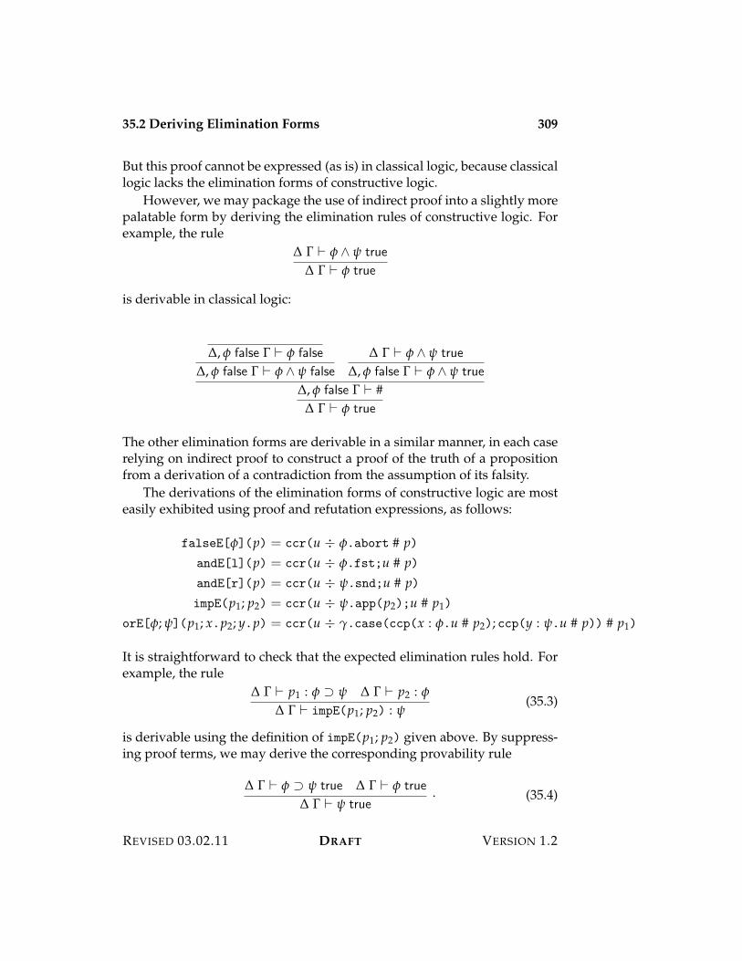
35.2 Deriving Elimination Forms 309
But this proof cannot be expressed (as is) in classical logic, because classicallogic lacks the elimination forms of constructive logic.
However, we may package the use of indirect proof into a slightly morepalatable form by deriving the elimination rules of constructive logic. Forexample, the rule
" ! ) ' 4 ( true
" ! ) ' true
is derivable in classical logic:
", ' false ! ) ' false
", ' false ! ) ' 4 ( false
" ! ) ' 4 ( true
", ' false ! ) ' 4 ( true
", ' false ! ) #" ! ) ' true
The other elimination forms are derivable in a similar manner, in each caserelying on indirect proof to construct a proof of the truth of a propositionfrom a derivation of a contradiction from the assumption of its falsity.
The derivations of the elimination forms of constructive logic are mosteasily exhibited using proof and refutation expressions, as follows:
falseE['](p) = ccr(u ÷ '.abort # p)andE[l](p) = ccr(u ÷ '.fst;u # p)andE[r](p) = ccr(u ÷ (.snd;u # p)impE(p1; p2) = ccr(u ÷ (.app(p2);u # p1)
orE['; (](p1; x.p2; y.p) = ccr(u ÷ /.case(ccp(x : '.u # p2); ccp(y : (.u # p)) # p1)
It is straightforward to check that the expected elimination rules hold. Forexample, the rule
" ! ) p1 : ' H ( " ! ) p2 : '
" ! ) impE(p1; p2) : ((35.3)
is derivable using the definition of impE(p1; p2) given above. By suppress-ing proof terms, we may derive the corresponding provability rule
" ! ) ' H ( true " ! ) ' true
" ! ) ( true. (35.4)
REVISED 03.02.11 DRAFT VERSION 1.2
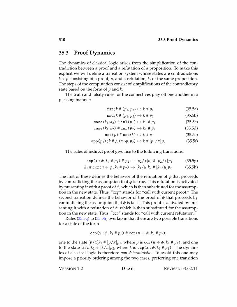
310 35.3 Proof Dynamics
35.3 Proof Dynamics
The dynamics of classical logic arises from the simplification of the con-tradiction between a proof and a refutation of a proposition. To make thisexplicit we will define a transition system whose states are contradictionsk # p consisting of a proof, p, and a refutation, k, of the same proposition.The steps of the computation consist of simplifications of the contradictorystate based on the form of p and k.
The truth and falsity rules for the connectives play off one another in apleasing manner:
fst;k # ?p1, p2@ 53 k # p1 (35.5a)snd;k # ?p1, p2@ 53 k # p2 (35.5b)
case(k1; k2) # inl(p1) 53 k1 # p1 (35.5c)case(k1; k2) # inr(p2) 53 k2 # p2 (35.5d)
not(p) # not(k) 53 k # p (35.5e)app(p1);k # ! (x:'. p2) 53 k # [p1/x]p2 (35.5f)
The rules of indirect proof give rise to the following transitions:
ccp(x : '.k1 # p1) # p2 53 [p2/x]k1 # [p2/x]p1 (35.5g)k1 # ccr(u ÷ '.k2 # p2) 53 [k1/u]k2 # [k1/u]p2 (35.5h)
The first of these defines the behavior of the refutation of ' that proceedsby contradicting the assumption that ' is true. This refutation is activatedby presenting it with a proof of ', which is then substituted for the assump-tion in the new state. Thus, “ccp” stands for “call with current proof.” Thesecond transition defines the behavior of the proof of ' that proceeds bycontradicting the assumption that ' is false. This proof is activated by pre-senting it with a refutation of ', which is then substituted for the assump-tion in the new state. Thus, “ccr” stands for “call with current refutation.”
Rules (35.5g) to (35.5h) overlap in that there are two possible transitionsfor a state of the form
ccp(x : '.k1 # p1) # ccr(u ÷ '.k2 # p2),
one to the state [p/x]k1 # [p/x]p1, where p is ccr(u ÷ '.k2 # p2), and oneto the state [k/u]k2 # [k/u]p2, where k is ccp(x : '.k1 # p1). The dynam-ics of classical logic is therefore non-deterministic. To avoid this one mayimpose a priority ordering among the two cases, preferring one transition
VERSION 1.2 DRAFT REVISED 03.02.11
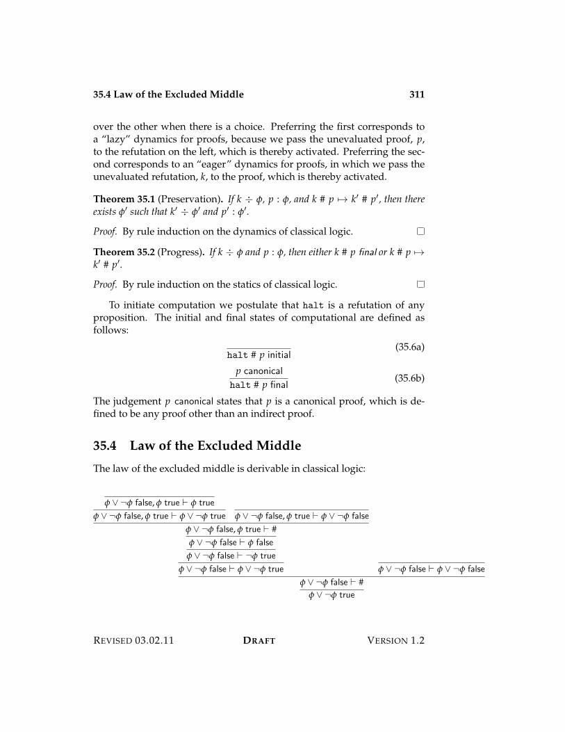
35.4 Law of the Excluded Middle 311
over the other when there is a choice. Preferring the first corresponds toa “lazy” dynamics for proofs, because we pass the unevaluated proof, p,to the refutation on the left, which is thereby activated. Preferring the sec-ond corresponds to an “eager” dynamics for proofs, in which we pass theunevaluated refutation, k, to the proof, which is thereby activated.
Theorem 35.1 (Preservation). If k ÷ ', p : ', and k # p 53 k% # p%, then thereexists '% such that k% ÷ '% and p% : '%.
Proof. By rule induction on the dynamics of classical logic.
Theorem 35.2 (Progress). If k ÷ ' and p : ', then either k # p final or k # p 53k% # p%.
Proof. By rule induction on the statics of classical logic.
To initiate computation we postulate that halt is a refutation of anyproposition. The initial and final states of computational are defined asfollows:
halt # p initial(35.6a)
p canonical
halt # p final(35.6b)
The judgement p canonical states that p is a canonical proof, which is de-fined to be any proof other than an indirect proof.
35.4 Law of the Excluded Middle
The law of the excluded middle is derivable in classical logic:
' G ¬' false, ' true ) ' true
' G ¬' false, ' true ) ' G ¬' true ' G ¬' false, ' true ) ' G ¬' false
' G ¬' false, ' true ) #' G ¬' false ) ' false
' G ¬' false ) ¬' true
' G ¬' false ) ' G ¬' true ' G ¬' false ) ' G ¬' false
' G ¬' false ) #' G ¬' true
REVISED 03.02.11 DRAFT VERSION 1.2
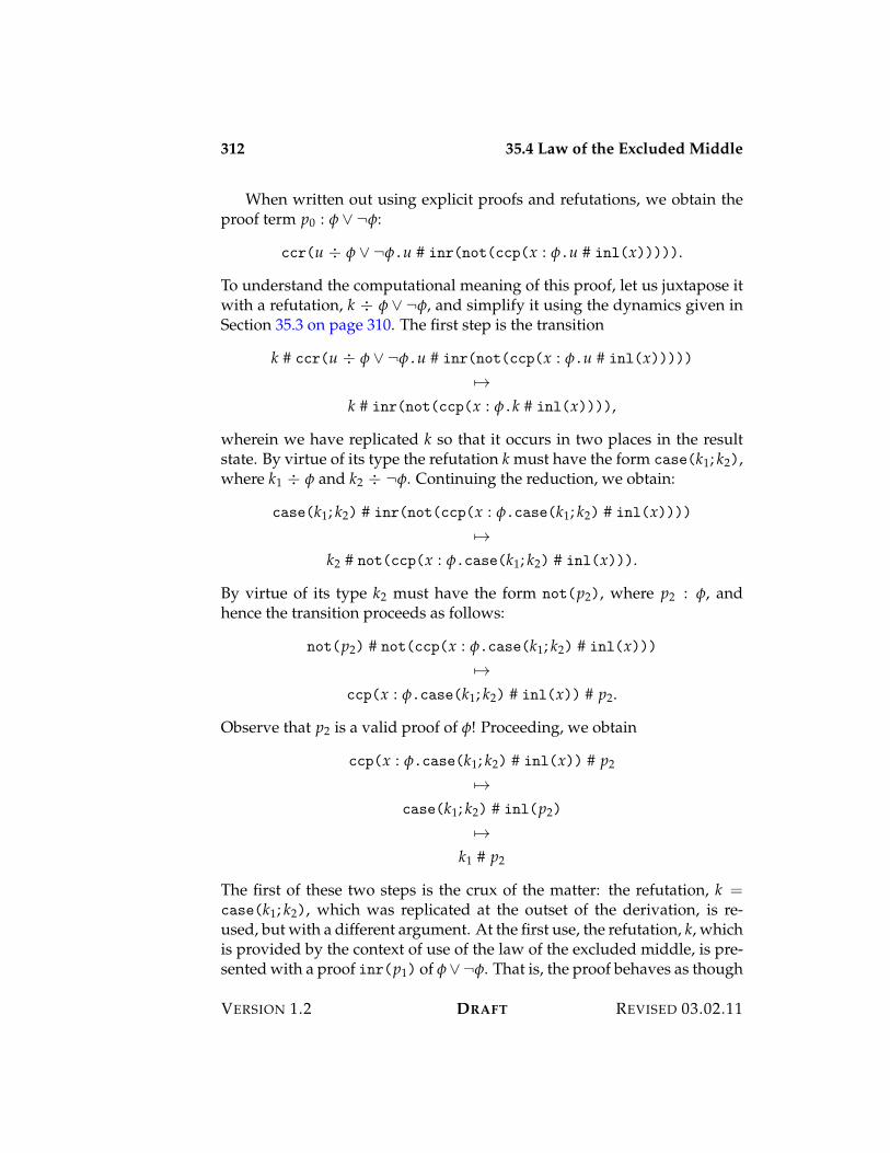
312 35.4 Law of the Excluded Middle
When written out using explicit proofs and refutations, we obtain theproof term p0 : ' G ¬':
ccr(u ÷ ' G ¬'.u # inr(not(ccp(x : '.u # inl(x))))).
To understand the computational meaning of this proof, let us juxtapose itwith a refutation, k ÷ ' G ¬', and simplify it using the dynamics given inSection 35.3 on page 310. The first step is the transition
k # ccr(u ÷ ' G ¬'.u # inr(not(ccp(x : '.u # inl(x)))))53
k # inr(not(ccp(x : '.k # inl(x)))),
wherein we have replicated k so that it occurs in two places in the resultstate. By virtue of its type the refutation k must have the form case(k1; k2),where k1 ÷ ' and k2 ÷ ¬'. Continuing the reduction, we obtain:
case(k1; k2) # inr(not(ccp(x : '.case(k1; k2) # inl(x))))53
k2 # not(ccp(x : '.case(k1; k2) # inl(x))).
By virtue of its type k2 must have the form not(p2), where p2 : ', andhence the transition proceeds as follows:
not(p2) # not(ccp(x : '.case(k1; k2) # inl(x)))53
ccp(x : '.case(k1; k2) # inl(x)) # p2.
Observe that p2 is a valid proof of '! Proceeding, we obtain
ccp(x : '.case(k1; k2) # inl(x)) # p2
53case(k1; k2) # inl(p2)
53k1 # p2
The first of these two steps is the crux of the matter: the refutation, k =case(k1; k2), which was replicated at the outset of the derivation, is re-used, but with a different argument. At the first use, the refutation, k, whichis provided by the context of use of the law of the excluded middle, is pre-sented with a proof inr(p1) of 'G¬'. That is, the proof behaves as though
VERSION 1.2 DRAFT REVISED 03.02.11
35.5 Exercises 313
the right disjunct of the law is true, which is to say that ' is false. If the con-text is such that it inspects this proof, it can only be by providing the proof,p2, of ' that refutes the claim that ' is false. Should this occur, the proofof the law of the excluded middle backtracks the context, providing insteadthe proof inl(p2) to k, which then passes p2 to k1 without further incident.The proof of the law of the excluded middle baldly asserts ¬' true, regard-less of the form of '. Then, if caught in its lie by the context providing aproof of ', changes its mind and asserts to the original context, k, after all!No further reversion is possible, because the context has itself provided aproof, p2, of '.
The law of the excluded middle illustrates that classical proofs are to bethought of as interactions between proofs and refutations, which is to sayinteractions between a proof and the context in which it is used. In pro-gramming terms this corresponds to an abstract machine with an explicitcontrol stack, or continuation, representing the context of evaluation of anexpression. That expression may access the context (stack, continuation)to effect backtracking as necessary to maintain the perfect symmetry be-tween truth and falsity. The penalty is that a closed proof of a disjunctionno longer need reveal which disjunct it proves, for as we have just seen, itmay, on further inspection, change its mind!
35.5 Exercises
REVISED 03.02.11 DRAFT VERSION 1.2

314 35.5 Exercises
VERSION 1.2 DRAFT REVISED 03.02.11

Part XIII
Symbols

Chapter 36
Symbols
A symbol is an atomic datum with no internal structure. Whereas variablesare given meaning by substitution, symbols are given meaning by a col-lection of primitives associated with it. In subsequent chapters we shallconsider several interpretations of symbols, giving rise to concepts such asfluid binding, dynamic classification, assignable variables, and communi-cation channels.
A “new “symbol, a, with associated type, &, is introduced within ascope, e, by the declaration new a:& in e. The meaning of the type & variesaccording to the interpretation of symbols under consideration. It is im-portant to emphasize, however, that a symbol is not a form of expression,and hence is not an element of its associated type. The expression, e, inthe symbol declaration new a:& in e, is the scope of the symbol. As usual,bound identifiers may be renamed within their scope, and hence a may beregarded as “new” in the sense that it may be chosen to be distinct fromany given finite set of symbols.
The dynamics of symbol declaration defines the extent, or range of sig-nificance, of the declared symbol. Under a scoped, or stack-like, dynamics,the extent of a symbol is just its scope. Once the scope of the declarationhas been evaluated, the symbol may be deallocated—the statics will ensurethat the result cannot depend on that symbol. Under a scope-free, or heap-like, dynamics the extent of a symbol is unlimited. A symbol may escapethe scope of its declaration, which means that it cannot be deallocated oncethe scope has been evaluated.
Perhaps the simplest application of symbols is as an atom that may becompared for equality with a given symbol. The type & sym has as elementssymbolic references of the form & a. The conditional if e is a then e1 ow be2
318 36.1 Symbol Declaration
branches according to whether e evaluates to & a or not, in a manner to bedescribed in more detail in Section 36.2 on page 321 below.
36.1 Symbol Declaration
The syntax for symbol declaration is given by the following grammar:
Expr e ::= new["](a.e) new a:" in e generation
Importantly, symbol declaration is not associated with any particular type,but is a primitive mechanism shared by all of the applications of symbols.
The statics of symbol declaration makes use of a signature, or symbolcontext, that associates a type to each of a finite set of symbols. We use theletter $ to range over signatures, which are finite sets of pairs a : ", wherea is a symbol and " is a type. The hypothetical typing judgement ! )$ e : "is parameterized by a signature, $, associating types to symbols.
The statics of symbol declaration is given by the following rule:
! )$,a:& e : " " mobile
! )$ new[&](a.e) : "(36.1)
It is implicit that a is chosen to not already be declared in $, ensuring thatit is not otherwise in use. The premise " mobile of Rule (36.1) specifies thatthe type, ", of the scope of the declaration must be mobile in the sense thatit is permissible to return a value of this type from the scope of a symboldeclaration.
The definition of mobility depends on the form of dynamics for sym-bol declaration. Under a scoped dynamics mobility is defined so that avalue of a mobile type cannot involve a symbol, and hence may safely bereturned from the scope of its declaration. This allows a symbol to be deal-located once it scope has been evaluated—that is, its extent coincides withits scope. Under a scope-free dynamics mobility imposes no restrictions onthe type, permitting any value, including one that depends on the declaredsymbol, to be returned from the scope of the declaration. To support thisthe dynamics must give symbols indefinite extent, even though they havestatic scope.
36.1.1 Scoped Dynamics
The scoped dynamics of symbol declaration is given by a transition judge-ment of the form e 5$3
$e% indexed by a signature, $, specifying the active
VERSION 1.2 DRAFT REVISED 03.02.11
36.1 Symbol Declaration 319
symbols of the transition. Either e or e% may involve the symbols declaredin $, but no others.
e 5$$3$,a:&
e%
new[&](a.e) 5$3$
new[&](a.e%)(36.2a)
e val$,a:& a /+ enew[&](a.e) 5$3
$e (36.2b)
Rule (36.2a) specifies that evaluation takes place within the scope of thedeclaration of a symbol. Rule (36.2b) specifies that the declared symbolmay be deallocated once its scope has been evaluated, provided that thedeclared symbol does not occur within that value. To ensure type safety, thedefinition of the judgement " mobile must be chosen so that this conditionalways holds.
36.1.2 Scope-Free Dynamics
The scope-free dynamics of symbols may be specified in one of two ways.One method is to consider a transition system between states of the form0 $ { e }, where $ is a signature and e is an expression over this signature.The judgement 0 $ { e } 53 0 $% { e% } states that evaluation of e relative tosymbols $ results in the expression e% in the extension $% of $.
a /+ dom($)0 $ { new[&](a.e) } 53 0 $, a : & { e }
(36.3)
Rule (36.3) specifies that symbol generation enriches the signature with thenewly introduced symbol by extending the signature for all future transi-tions.
Such a formulation of the dynamics is disadvantageous because it relieson an extra-linguistic notion of the state of the computation. One conse-quence is that the dynamics of all other aspects of the language must bereformulated to account for this change. For example, the dynamics of (by-name) function application cannot simply be inherited from Chapter 13,but must instead be re-formulated as follows:
0 $ { e1 } 53 0 $% { e%1 }0 $ { e1(e2) } 53 0 $% { e%1(e2) }
(36.4a)
0 $ { ! (x:". e)(e2) } 53 0 $ { [e2/x]e }(36.4b)
REVISED 03.02.11 DRAFT VERSION 1.2
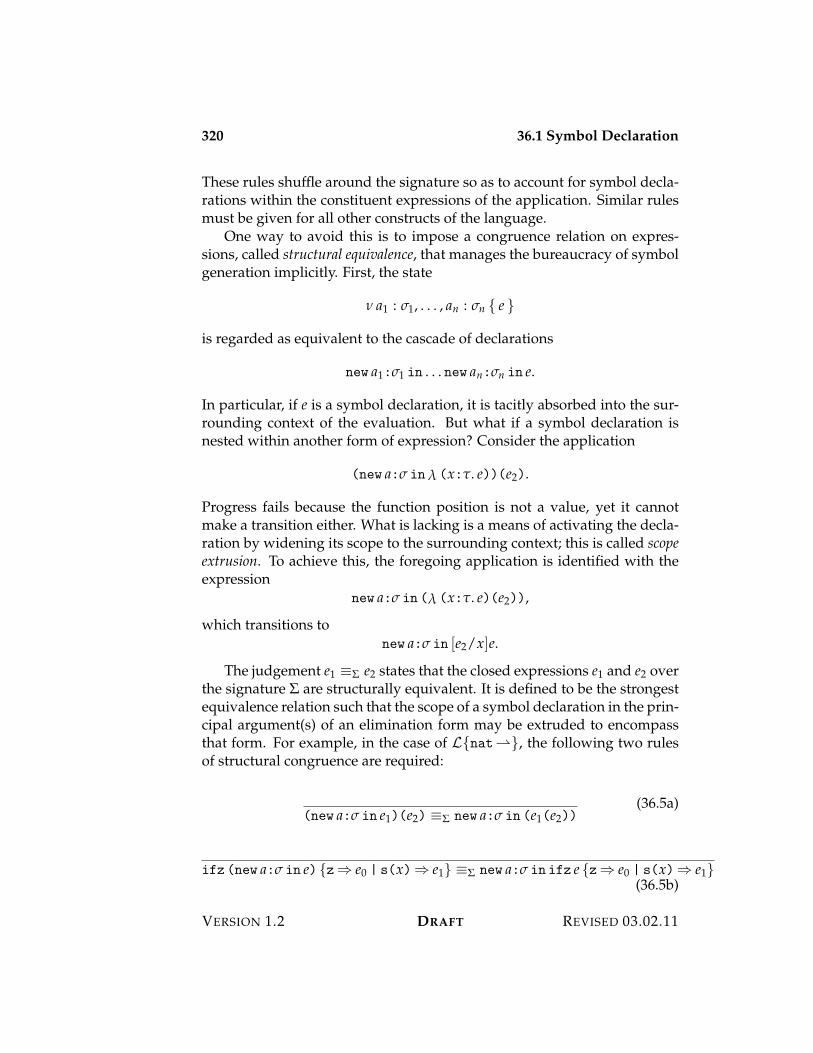
320 36.1 Symbol Declaration
These rules shuffle around the signature so as to account for symbol decla-rations within the constituent expressions of the application. Similar rulesmust be given for all other constructs of the language.
One way to avoid this is to impose a congruence relation on expres-sions, called structural equivalence, that manages the bureaucracy of symbolgeneration implicitly. First, the state
0 a1 : &1, . . . , an : &n { e }
is regarded as equivalent to the cascade of declarations
new a1:&1 in . . . new an:&n in e.
In particular, if e is a symbol declaration, it is tacitly absorbed into the sur-rounding context of the evaluation. But what if a symbol declaration isnested within another form of expression? Consider the application
(new a:& in! (x:". e))(e2).
Progress fails because the function position is not a value, yet it cannotmake a transition either. What is lacking is a means of activating the decla-ration by widening its scope to the surrounding context; this is called scopeextrusion. To achieve this, the foregoing application is identified with theexpression
new a:& in (! (x:". e)(e2)),
which transitions tonew a:& in [e2/x]e.
The judgement e1 9$ e2 states that the closed expressions e1 and e2 overthe signature $ are structurally equivalent. It is defined to be the strongestequivalence relation such that the scope of a symbol declaration in the prin-cipal argument(s) of an elimination form may be extruded to encompassthat form. For example, in the case of L{nat"}, the following two rulesof structural congruence are required:
(new a:& in e1)(e2) 9$ new a:& in (e1(e2))(36.5a)
ifz (new a:& in e) {z; e0 | s(x); e1} 9$ new a:& in ifz e {z; e0 | s(x); e1}(36.5b)
VERSION 1.2 DRAFT REVISED 03.02.11

36.2 Symbolic References 321
Crucially, the dynamics is defined to respect structural equivalence:
e1 9$ e2 e2 5$3$
e%2 e%2 9$ e%1
e1 5$3$
e%1(36.6)
A technical lemma states that structurally equivalent expressions havethe same types.
Lemma 36.1. If e1 9$ e2, then )$ e1 : " iff )$ e2 : ".
Theorem 36.2 (Preservation). If )$ e : " and e 5$3$
e%, then e% : ".
Proof. The interesting case is Rule (36.6), for which we appeal to Lemma 36.1.
Theorem 36.3 (Progress). If )$ e : ", then either there exists n 7 0 such thate 9$ new a1:&1 in . . . new an:&n in e% with e% val$,a1:&1,...,an :&n , or there exists e%such that e 5$3
$e%.
Proof. By induction on typing, making use of scope extrusion. For ex-ample, suppose that e is e1(e2), where )$ e1 : "2 3 " and )$ e2 : "2.By induction with have that either e1 9$ new a1:&1 in . . . new an:&n in e%1,where e%1 val$,a1:&1,...,an :&n , or e 5$3
$e% for some e%. In the latter case appeal
to Rule (36.2a). In the former, apply Rule (36.5a) to show that e1(e2) 9$new a1:&1 in . . . new an:&n in e%1(e2), then apply Rule (36.6) and the canoni-cal forms lemma for function types.
36.2 Symbolic References
As discussed in the introduction to this chapter, the type " sym has as valuessymbolic references, & a, to a symbol, a. Given such a value, we may branchon whether it is a reference to a specified symbol or not. The syntax of theseprimitives is given by the following grammar:
Type " ::= sym(") " sym symbolic referenceExpr e sym[a] & a symbolic reference
is[a][t."](e; e1; e2) comparisonif e is a then e1 ow be2
The expression sym[a] is a reference to the symbol a, a value of type sym(").The expression is[a][t."](e; e1; e2) compares the value of e, which mustbe a reference to some symbol b, with the given symbol, a. If b is a, theexpression evaluates to e1, and otherwise to e2.
REVISED 03.02.11 DRAFT VERSION 1.2
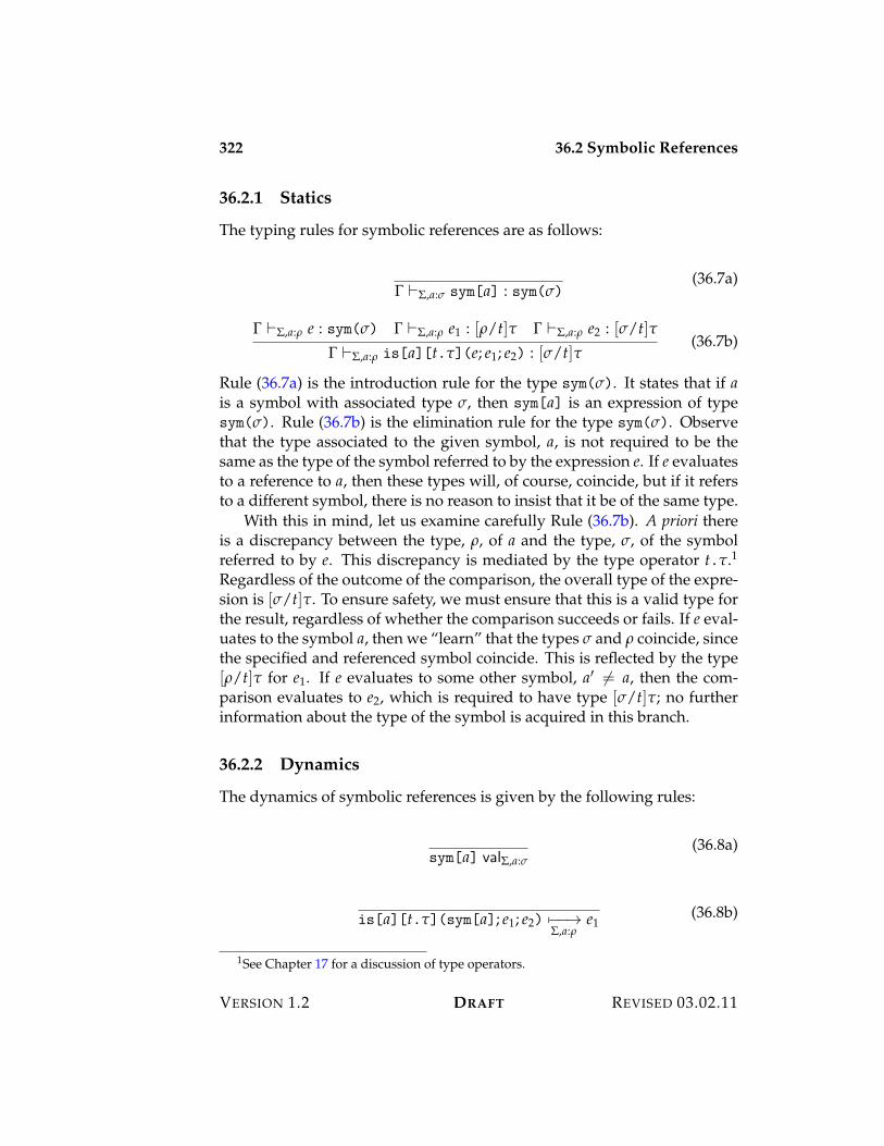
322 36.2 Symbolic References
36.2.1 Statics
The typing rules for symbolic references are as follows:
! )$,a:& sym[a] : sym(&)(36.7a)
! )$,a:, e : sym(&) ! )$,a:, e1 : [,/t]" ! )$,a:, e2 : [&/t]"! )$,a:, is[a][t."](e; e1; e2) : [&/t]"
(36.7b)
Rule (36.7a) is the introduction rule for the type sym(&). It states that if ais a symbol with associated type &, then sym[a] is an expression of typesym(&). Rule (36.7b) is the elimination rule for the type sym(&). Observethat the type associated to the given symbol, a, is not required to be thesame as the type of the symbol referred to by the expression e. If e evaluatesto a reference to a, then these types will, of course, coincide, but if it refersto a different symbol, there is no reason to insist that it be of the same type.
With this in mind, let us examine carefully Rule (36.7b). A priori thereis a discrepancy between the type, ,, of a and the type, &, of the symbolreferred to by e. This discrepancy is mediated by the type operator t.".1Regardless of the outcome of the comparison, the overall type of the expre-sion is [&/t]". To ensure safety, we must ensure that this is a valid type forthe result, regardless of whether the comparison succeeds or fails. If e eval-uates to the symbol a, then we “learn” that the types & and , coincide, sincethe specified and referenced symbol coincide. This is reflected by the type[,/t]" for e1. If e evaluates to some other symbol, a% ,= a, then the com-parison evaluates to e2, which is required to have type [&/t]"; no furtherinformation about the type of the symbol is acquired in this branch.
36.2.2 Dynamics
The dynamics of symbolic references is given by the following rules:
sym[a] val$,a:&(36.8a)
is[a][t."](sym[a]; e1; e2) 5$$3$,a:,
e1(36.8b)
1See Chapter 17 for a discussion of type operators.
VERSION 1.2 DRAFT REVISED 03.02.11
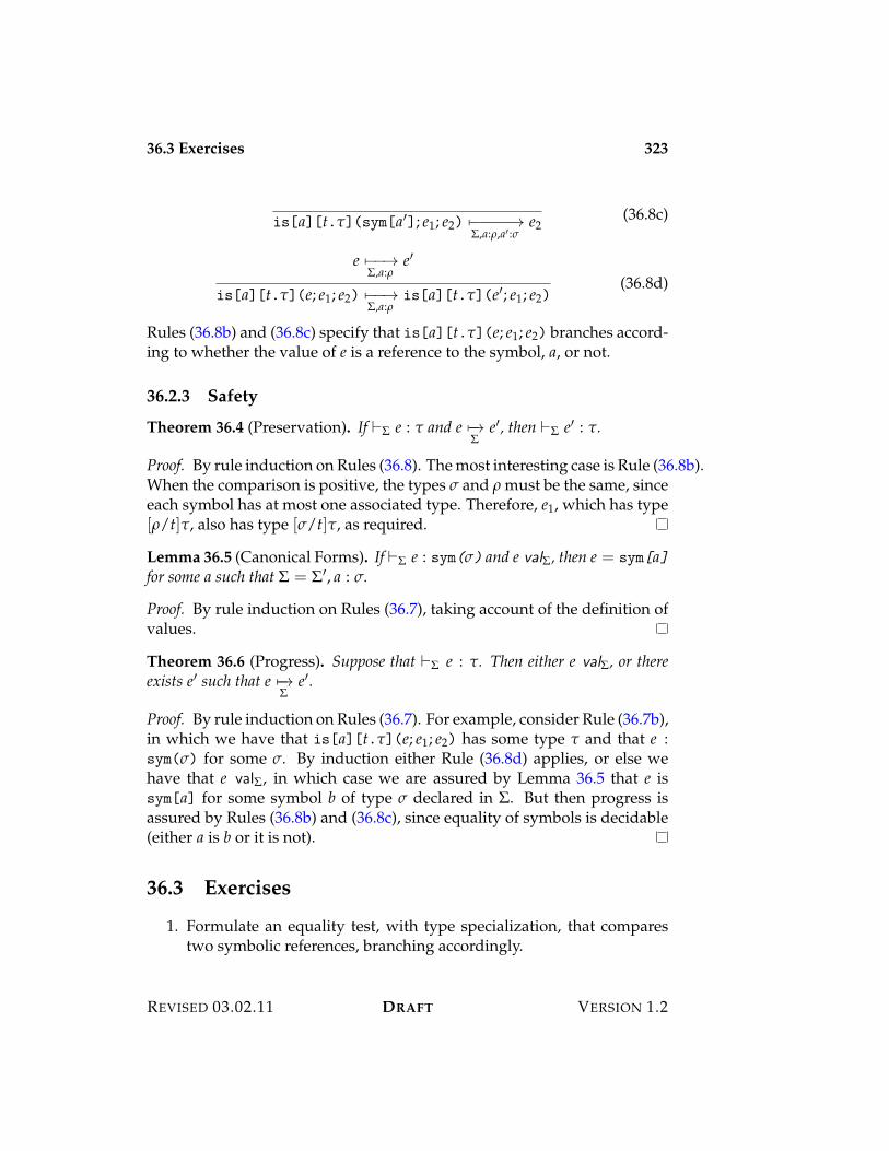
36.3 Exercises 323
is[a][t."](sym[a%]; e1; e2) 5$$$$3$,a:,,a% :&
e2(36.8c)
e 5$$3$,a:,
e%
is[a][t."](e; e1; e2) 5$$3$,a:,
is[a][t."](e%; e1; e2)(36.8d)
Rules (36.8b) and (36.8c) specify that is[a][t."](e; e1; e2) branches accord-ing to whether the value of e is a reference to the symbol, a, or not.
36.2.3 Safety
Theorem 36.4 (Preservation). If )$ e : " and e 5$3$
e%, then )$ e% : ".
Proof. By rule induction on Rules (36.8). The most interesting case is Rule (36.8b).When the comparison is positive, the types & and , must be the same, sinceeach symbol has at most one associated type. Therefore, e1, which has type[,/t]", also has type [&/t]", as required.
Lemma 36.5 (Canonical Forms). If )$ e : sym(&) and e val$, then e = sym[a]for some a such that $ = $%, a : &.
Proof. By rule induction on Rules (36.7), taking account of the definition ofvalues.
Theorem 36.6 (Progress). Suppose that )$ e : ". Then either e val$, or thereexists e% such that e 5$3
$e%.
Proof. By rule induction on Rules (36.7). For example, consider Rule (36.7b),in which we have that is[a][t."](e; e1; e2) has some type " and that e :sym(&) for some &. By induction either Rule (36.8d) applies, or else wehave that e val$, in which case we are assured by Lemma 36.5 that e issym[a] for some symbol b of type & declared in $. But then progress isassured by Rules (36.8b) and (36.8c), since equality of symbols is decidable(either a is b or it is not).
36.3 Exercises
1. Formulate an equality test, with type specialization, that comparestwo symbolic references, branching accordingly.
REVISED 03.02.11 DRAFT VERSION 1.2

324 36.3 Exercises
VERSION 1.2 DRAFT REVISED 03.02.11
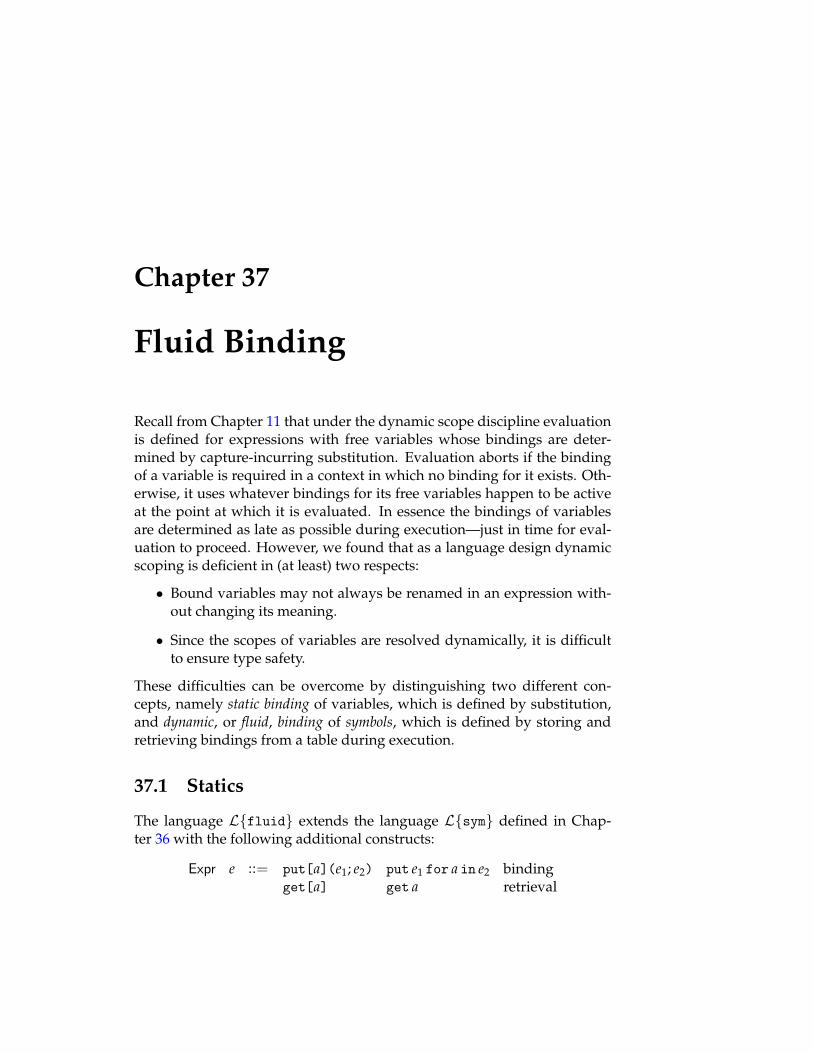
Chapter 37
Fluid Binding
Recall from Chapter 11 that under the dynamic scope discipline evaluationis defined for expressions with free variables whose bindings are deter-mined by capture-incurring substitution. Evaluation aborts if the bindingof a variable is required in a context in which no binding for it exists. Oth-erwise, it uses whatever bindings for its free variables happen to be activeat the point at which it is evaluated. In essence the bindings of variablesare determined as late as possible during execution—just in time for eval-uation to proceed. However, we found that as a language design dynamicscoping is deficient in (at least) two respects:
• Bound variables may not always be renamed in an expression with-out changing its meaning.
• Since the scopes of variables are resolved dynamically, it is difficultto ensure type safety.
These difficulties can be overcome by distinguishing two different con-cepts, namely static binding of variables, which is defined by substitution,and dynamic, or fluid, binding of symbols, which is defined by storing andretrieving bindings from a table during execution.
37.1 Statics
The language L{fluid} extends the language L{sym} defined in Chap-ter 36 with the following additional constructs:
Expr e ::= put[a](e1; e2) put e1 for a in e2 bindingget[a] get a retrieval
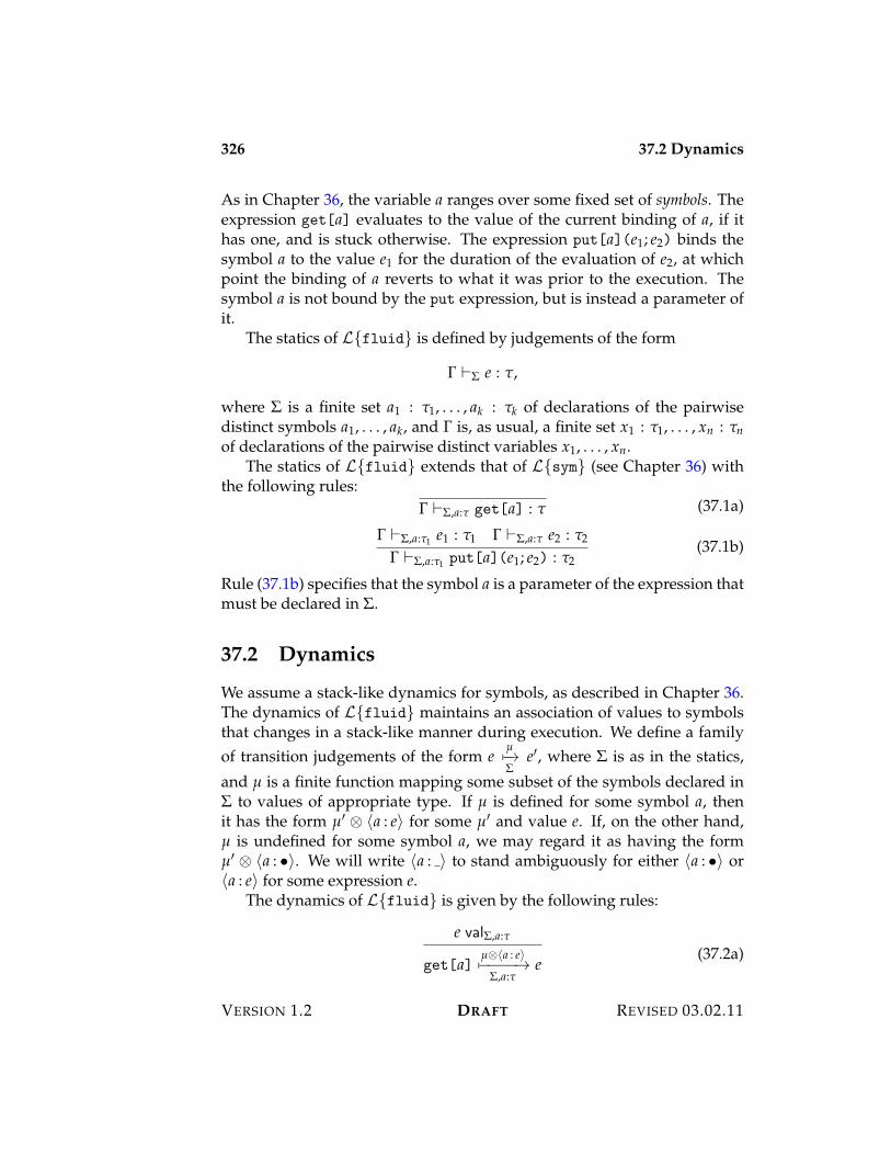
326 37.2 Dynamics
As in Chapter 36, the variable a ranges over some fixed set of symbols. Theexpression get[a] evaluates to the value of the current binding of a, if ithas one, and is stuck otherwise. The expression put[a](e1; e2) binds thesymbol a to the value e1 for the duration of the evaluation of e2, at whichpoint the binding of a reverts to what it was prior to the execution. Thesymbol a is not bound by the put expression, but is instead a parameter ofit.
The statics of L{fluid} is defined by judgements of the form
! )$ e : ",
where $ is a finite set a1 : "1, . . . , ak : "k of declarations of the pairwisedistinct symbols a1, . . . , ak, and ! is, as usual, a finite set x1 : "1, . . . , xn : "nof declarations of the pairwise distinct variables x1, . . . , xn.
The statics of L{fluid} extends that of L{sym} (see Chapter 36) withthe following rules:
! )$,a:" get[a] : " (37.1a)
! )$,a:"1 e1 : "1 ! )$,a:" e2 : "2
! )$,a:"1 put[a](e1; e2) : "2(37.1b)
Rule (37.1b) specifies that the symbol a is a parameter of the expression thatmust be declared in $.
37.2 Dynamics
We assume a stack-like dynamics for symbols, as described in Chapter 36.The dynamics of L{fluid} maintains an association of values to symbolsthat changes in a stack-like manner during execution. We define a familyof transition judgements of the form e
µ5$3$
e%, where $ is as in the statics,and µ is a finite function mapping some subset of the symbols declared in$ to values of appropriate type. If µ is defined for some symbol a, thenit has the form µ% E ?a : e@ for some µ% and value e. If, on the other hand,µ is undefined for some symbol a, we may regard it as having the formµ% E ?a : •@. We will write ?a : @ to stand ambiguously for either ?a : •@ or?a : e@ for some expression e.
The dynamics of L{fluid} is given by the following rules:
e val$,a:"
get[a]µE?a : e@5$$$$3
$,a:"e
(37.2a)
VERSION 1.2 DRAFT REVISED 03.02.11
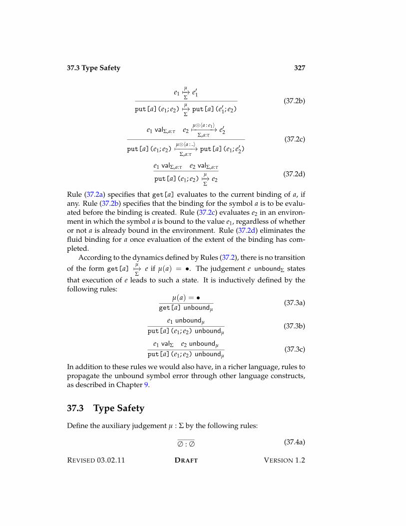
37.3 Type Safety 327
e1µ5$3$
e%1
put[a](e1; e2)µ5$3$
put[a](e%1; e2)(37.2b)
e1 val$,a:" e2µE?a : e1@5$$$$$3
$,a:"e%2
put[a](e1; e2)µE?a : @5$$$$3
$,a:"put[a](e1; e%2)
(37.2c)
e1 val$,a:" e2 val$,a:"
put[a](e1; e2)µ5$3$
e2(37.2d)
Rule (37.2a) specifies that get[a] evaluates to the current binding of a, ifany. Rule (37.2b) specifies that the binding for the symbol a is to be evalu-ated before the binding is created. Rule (37.2c) evaluates e2 in an environ-ment in which the symbol a is bound to the value e1, regardless of whetheror not a is already bound in the environment. Rule (37.2d) eliminates thefluid binding for a once evaluation of the extent of the binding has com-pleted.
According to the dynamics defined by Rules (37.2), there is no transitionof the form get[a]
µ5$3$
e if µ(a) = •. The judgement e unbound$ statesthat execution of e leads to such a state. It is inductively defined by thefollowing rules:
µ(a) = •get[a] unboundµ
(37.3a)
e1 unboundµ
put[a](e1; e2) unboundµ(37.3b)
e1 val$ e2 unboundµ
put[a](e1; e2) unboundµ(37.3c)
In addition to these rules we would also have, in a richer language, rules topropagate the unbound symbol error through other language constructs,as described in Chapter 9.
37.3 Type Safety
Define the auxiliary judgement µ : $ by the following rules:
# : # (37.4a)
REVISED 03.02.11 DRAFT VERSION 1.2
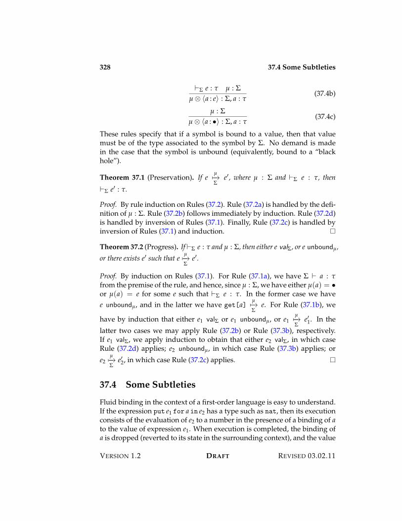
328 37.4 Some Subtleties
)$ e : " µ : $µ E ?a : e@ : $, a : "
(37.4b)
µ : $µ E ?a : •@ : $, a : "
(37.4c)
These rules specify that if a symbol is bound to a value, then that valuemust be of the type associated to the symbol by $. No demand is madein the case that the symbol is unbound (equivalently, bound to a “blackhole”).
Theorem 37.1 (Preservation). If eµ5$3$
e%, where µ : $ and )$ e : ", then
)$ e% : ".
Proof. By rule induction on Rules (37.2). Rule (37.2a) is handled by the defi-nition of µ : $. Rule (37.2b) follows immediately by induction. Rule (37.2d)is handled by inversion of Rules (37.1). Finally, Rule (37.2c) is handled byinversion of Rules (37.1) and induction.
Theorem 37.2 (Progress). If )$ e : " and µ : $, then either e val$, or e unboundµ,or there exists e% such that e
µ5$3$
e%.
Proof. By induction on Rules (37.1). For Rule (37.1a), we have $ ) a : "from the premise of the rule, and hence, since µ : $, we have either µ(a) = •or µ(a) = e for some e such that )$ e : ". In the former case we havee unboundµ, and in the latter we have get[a]
µ5$3$
e. For Rule (37.1b), we
have by induction that either e1 val$ or e1 unboundµ, or e1µ5$3$
e%1. In thelatter two cases we may apply Rule (37.2b) or Rule (37.3b), respectively.If e1 val$, we apply induction to obtain that either e2 val$, in which caseRule (37.2d) applies; e2 unboundµ, in which case Rule (37.3b) applies; ore2
µ5$3$
e%2, in which case Rule (37.2c) applies.
37.4 Some Subtleties
Fluid binding in the context of a first-order language is easy to understand.If the expression put e1 for a in e2 has a type such as nat, then its executionconsists of the evaluation of e2 to a number in the presence of a binding of ato the value of expression e1. When execution is completed, the binding ofa is dropped (reverted to its state in the surrounding context), and the value
VERSION 1.2 DRAFT REVISED 03.02.11
37.4 Some Subtleties 329
is returned. Since this value is a number, it cannot contain any reference toa, and so no issue of its binding arises.
But what if the type of put e1 for a in e2 is a function type, so that thereturned value is a !-abstraction? In that case the body of the ! may containreferences to the symbol a whose binding is dropped upon return. Thisraises an important question about the interaction between fluid bindingand higher-order functions. For example, consider the expression
put 17 for a in! (x:nat. x + get a), (37.5)
which has type nat, given that a is a symbol of the same type. Let us as-sume, for the sake of discussion, that a is unbound at the point at which thisexpression is evaluated. Doing so binds a to the number 17, and returns thefunction ! (x:nat. x + get a). This function contains the symbol a, but isreturned to a context in which the symbol a is not bound. This means that,for example, application of the expression (37.5) to an argument will incuran error because the symbol a is not bound.
Contrast this with the similar expression
let y be 17 in! (x:nat. x + y), (37.6)
in which we have replaced the fluid-bound symbol, a, by a statically boundvariable, y. This expression evaluates to ! (x:nat. x + 17), which adds 17to its argument when applied. There is never any possibility of an un-bound symbol arising at execution time, precisely because the identifica-tion of scope and extent ensures that the association between a variableand its binding is never violated.
It is hard to say whether either of these two behaviors is “right” or“wrong.” Static binding is an important mechanism for encapsulation ofbehavior in a program; without static binding, one cannot ensure that themeaning of a variable is unchanged by the context in which it is used. Dy-namic binding is used to avoid passing arguments to a function in orderto specialize its behavior. Instead we rely on fluid binding to establish thebinding of a symbol for the duration of execution of the function, avoidingthe need to re-bind the fluids at each call site.
For example, let e stand for the value of expression (37.5), a !-abstractionwhose body is dependent on the binding of the symbol a. This imposes therequirement that the programmer provide a binding for a whenever e isapplied to an argument. For example, the expression
put 7 for a in (e(9))
REVISED 03.02.11 DRAFT VERSION 1.2
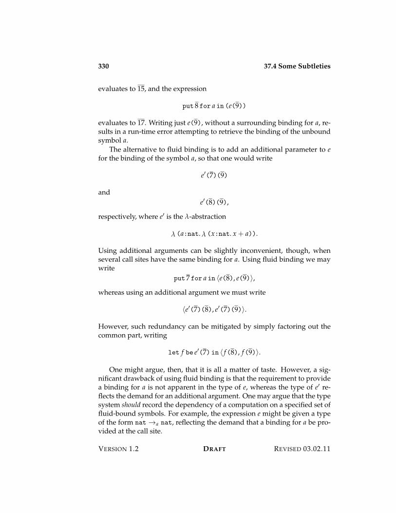
330 37.4 Some Subtleties
evaluates to 15, and the expression
put 8 for a in (e(9))
evaluates to 17. Writing just e(9), without a surrounding binding for a, re-sults in a run-time error attempting to retrieve the binding of the unboundsymbol a.
The alternative to fluid binding is to add an additional parameter to efor the binding of the symbol a, so that one would write
e%(7)(9)
ande%(8)(9),
respectively, where e% is the !-abstraction
! (a:nat. ! (x:nat. x + a)).
Using additional arguments can be slightly inconvenient, though, whenseveral call sites have the same binding for a. Using fluid binding we maywrite
put 7 for a in ?e(8), e(9)@,
whereas using an additional argument we must write
?e%(7)(8), e%(7)(9)@.
However, such redundancy can be mitigated by simply factoring out thecommon part, writing
let f be e%(7) in ? f(8), f(9)@.
One might argue, then, that it is all a matter of taste. However, a sig-nificant drawback of using fluid binding is that the requirement to providea binding for a is not apparent in the type of e, whereas the type of e% re-flects the demand for an additional argument. One may argue that the typesystem should record the dependency of a computation on a specified set offluid-bound symbols. For example, the expression e might be given a typeof the form nat 3a nat, reflecting the demand that a binding for a be pro-vided at the call site.
VERSION 1.2 DRAFT REVISED 03.02.11
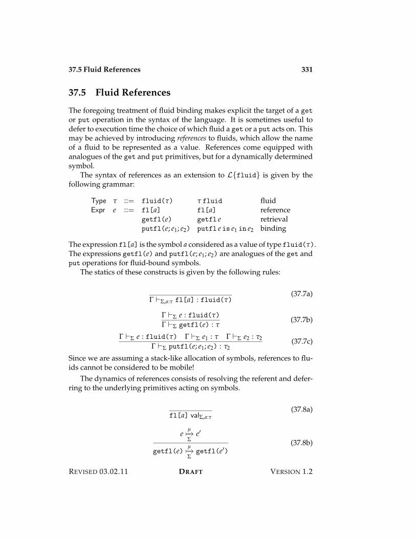
37.5 Fluid References 331
37.5 Fluid References
The foregoing treatment of fluid binding makes explicit the target of a get
or put operation in the syntax of the language. It is sometimes useful todefer to execution time the choice of which fluid a get or a put acts on. Thismay be achieved by introducing references to fluids, which allow the nameof a fluid to be represented as a value. References come equipped withanalogues of the get and put primitives, but for a dynamically determinedsymbol.
The syntax of references as an extension to L{fluid} is given by thefollowing grammar:
Type " ::= fluid(") " fluid fluidExpr e ::= fl[a] fl[a] reference
getfl(e) getfl e retrievalputfl(e; e1; e2) putfl e is e1 in e2 binding
The expression fl[a] is the symbol a considered as a value of type fluid(").The expressions getfl(e) and putfl(e; e1; e2) are analogues of the get andput operations for fluid-bound symbols.
The statics of these constructs is given by the following rules:
! )$,a:" fl[a] : fluid(")(37.7a)
! )$ e : fluid(")! )$ getfl(e) : "
(37.7b)
! )$ e : fluid(") ! )$ e1 : " ! )$ e2 : "2! )$ putfl(e; e1; e2) : "2
(37.7c)
Since we are assuming a stack-like allocation of symbols, references to flu-ids cannot be considered to be mobile!
The dynamics of references consists of resolving the referent and defer-ring to the underlying primitives acting on symbols.
fl[a] val$,a:"(37.8a)
eµ5$3$
e%
getfl(e)µ5$3$
getfl(e%)(37.8b)
REVISED 03.02.11 DRAFT VERSION 1.2
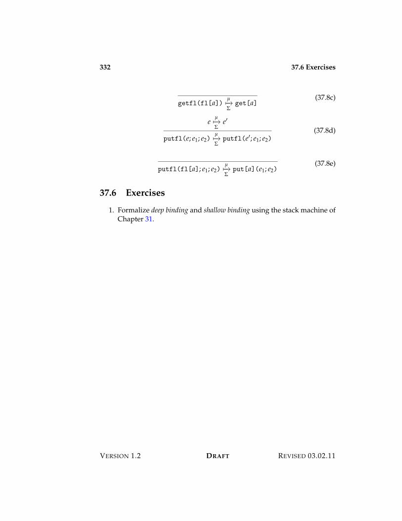
332 37.6 Exercises
getfl(fl[a])µ5$3$
get[a](37.8c)
eµ5$3$
e%
putfl(e; e1; e2)µ5$3$
putfl(e%; e1; e2)(37.8d)
putfl(fl[a]; e1; e2)µ5$3$
put[a](e1; e2)(37.8e)
37.6 Exercises
1. Formalize deep binding and shallow binding using the stack machine ofChapter 31.
VERSION 1.2 DRAFT REVISED 03.02.11
Chapter 38
Dynamic Classification
In Chapters 15 and 29 we investigated the use of sums for the classificationof values of disparate type. Every value of a classified type is labelled witha symbol that determines the type of the instance data. A classified value isdecomposed by pattern matching against a known class, which reveals thetype of the instance data.
Under this representation the possible classes of an object are fully de-termined statically by its type. However, it is sometimes useful to allow thepossible classes of data value to be determined dynamically. A typical situa-tion of this kind arises when two components of a program wish to “sharea secret”—that is, to compute a value that is opaque to intermediaries. Thiscan be accomplished by creating a fresh class that is known only to the two“end points” of the communication who may create instances of this class,and pattern match against it to recover the underlying datum. In this sensedynamic classification may be regarded as a perfect encryption mechanism inwhich the class serves as an absolutely unbreakable encryption key underwhich data may be protected from intruders. It is absolutely unbreakablebecause, by $-equivalence, it is impossible to “guess” the name of a boundsymbol.1
One may wonder why a program would ever need to keep a secretfrom itself. There are, in fact, many useful applications of such an idea.For example, a program may consist of many independent processes com-municating over an insecure network. Perfect encryption by dynamic clas-sification supports the creation of private channels between processes; see
1In practice this is implemented using probabilistic techniques to avoid the need for acentral arbiter of unicity of symbol names. However, such methods require a source ofrandomness, which may be seen as just such an arbiter in disguise. There is no free lunch.
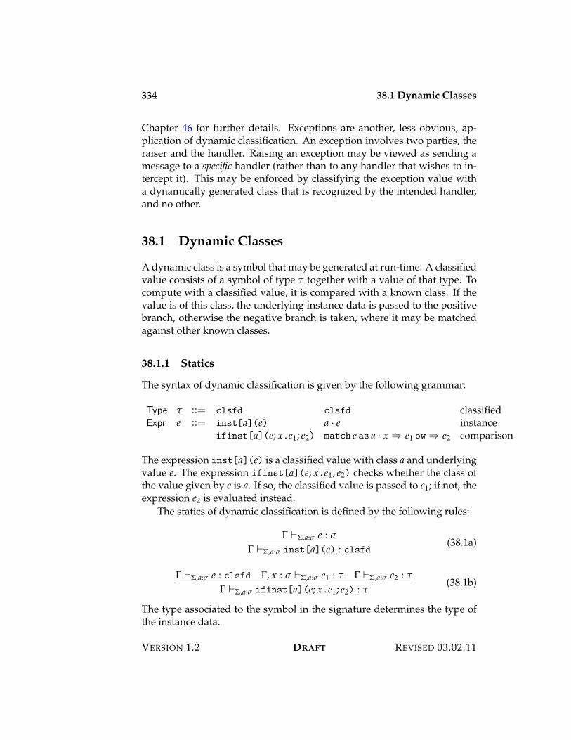
334 38.1 Dynamic Classes
Chapter 46 for further details. Exceptions are another, less obvious, ap-plication of dynamic classification. An exception involves two parties, theraiser and the handler. Raising an exception may be viewed as sending amessage to a specific handler (rather than to any handler that wishes to in-tercept it). This may be enforced by classifying the exception value witha dynamically generated class that is recognized by the intended handler,and no other.
38.1 Dynamic Classes
A dynamic class is a symbol that may be generated at run-time. A classifiedvalue consists of a symbol of type " together with a value of that type. Tocompute with a classified value, it is compared with a known class. If thevalue is of this class, the underlying instance data is passed to the positivebranch, otherwise the negative branch is taken, where it may be matchedagainst other known classes.
38.1.1 Statics
The syntax of dynamic classification is given by the following grammar:
Type " ::= clsfd clsfd classifiedExpr e ::= inst[a](e) a · e instance
ifinst[a](e; x.e1; e2) match e as a · x ; e1 ow ; e2 comparison
The expression inst[a](e) is a classified value with class a and underlyingvalue e. The expression ifinst[a](e; x.e1; e2) checks whether the class ofthe value given by e is a. If so, the classified value is passed to e1; if not, theexpression e2 is evaluated instead.
The statics of dynamic classification is defined by the following rules:
! )$,a:& e : &
! )$,a:& inst[a](e) : clsfd(38.1a)
! )$,a:& e : clsfd !, x : & )$,a:& e1 : " ! )$,a:& e2 : "
! )$,a:& ifinst[a](e; x.e1; e2) : "(38.1b)
The type associated to the symbol in the signature determines the type ofthe instance data.
VERSION 1.2 DRAFT REVISED 03.02.11
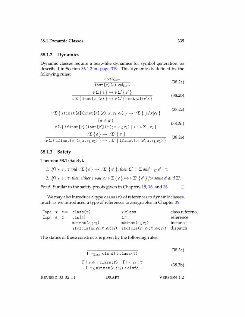
38.1 Dynamic Classes 335
38.1.2 Dynamics
Dynamic classes require a heap-like dynamics for symbol generation, asdescribed in Section 36.1.2 on page 319. This dynamics is defined by thefollowing rules:
e val$,a:"
inst[a](e) val$,a:"(38.2a)
0 $ { e } 53 0 $% { e% }0 $ { inst[a](e) } 53 0 $% { inst[a](e%) }
(38.2b)
0 $ { ifinst[a](inst[a](e); x.e1; e2) } 53 0 $ { [e/x]e1 }(38.2c)
(a ,= a%)0 $ { ifinst[a](inst[a%](e%); x.e1; e2) } 53 0 $ { e2 }
(38.2d)
0 $ { e } 53 0 $% { e% }0 $ { ifinst[a](e; x.e1; e2) } 53 0 $% { ifinst[a](e%; x.e1; e2) }
(38.2e)
38.1.3 Safety
Theorem 38.1 (Safety).
1. If )$ e : " and 0 $ { e } 53 0 $% { e% }, then $% L $ and )$% e% : ".
2. If )$ e : ", then either e val$ or 0 $ { e } 53 0 $% { e% } for some e% and $%.
Proof. Similar to the safety proofs given in Chapters 15, 16, and 36.
We may also introduce a type class(") of references to dynamic classes,much as we introduced a type of references to assignables in Chapter 39.
Type " ::= class(") " class class referenceExpr e ::= cls[a] & a reference
mkinst(e1; e2) mkinst(e1; e2) instanceifofcls(e0; e1; x.e2; e3) ifofcls(e0; e1; x.e2; e3) dispatch
The statics of these constructs is given by the following rules:
! )$,a:" cls[a] : class(")(38.3a)
! )$ e1 : class(") ! )$ e2 : "! )$ mkinst(e1; e2) : clsfd
(38.3b)
REVISED 03.02.11 DRAFT VERSION 1.2
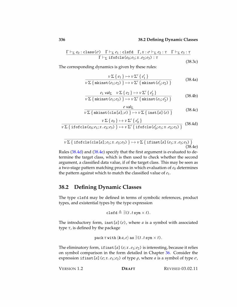
336 38.2 Defining Dynamic Classes
! )$ e0 : class(&) ! )$ e1 : clsfd !, x : & )$ e2 : " ! )$ e3 : "! )$ ifofcls(e0; e1; x.e2; e3) : "
(38.3c)The corresponding dynamics is given by these rules:
0 $ { e1 } 53 0 $% { e%1 }0 $ { mkinst(e1; e2) } 53 0 $% { mkinst(e%1; e2) }
(38.4a)
e1 val$ 0 $ { e2 } 53 0 $% { e%2 }0 $ { mkinst(e1; e2) } 53 0 $% { mkinst(e1; e%2) }
(38.4b)
e val$0 $ { mkinst(cls[a]; e) } 53 0 $ { inst[a](e) } (38.4c)
0 $ { e0 } 53 0 $% { e%0 }0 $ { ifofcls(e0; e1; x.e2; e3) } 53 0 $% { ifofcls(e%0; e1; x.e2; e3) }
(38.4d)
0 $ { ifofcls(cls[a]; e1; x.e2; e3) } 53 0 $ { ifinst[a](e1; x.e2; e3) }(38.4e)
Rules (38.4d) and (38.4e) specify that the first argument is evaluated to de-termine the target class, which is then used to check whether the secondargument, a classified data value, if of the target class. This may be seen asa two-stage pattern matching process in which evaluation of e0 determinesthe pattern against which to match the classified value of e1.
38.2 Defining Dynamic Classes
The type clsfd may be defined in terms of symbolic references, producttypes, and existential types by the type expression
clsfd % '(t.t sym< t).
The introductory form, inst[a](e), where a is a symbol with associatedtype ", is defined by the package
pack " with ?& a, e@ as '(t.t sym< t).
The eliminatory form, ifinst[a](e; x.e1; e2) is interesting, because it relieson symbol comparison in the form detailed in Chapter 36. Consider theexpression ifinst[a](e; x.e1; e2) of type ,, where a is a symbol of type &,
VERSION 1.2 DRAFT REVISED 03.02.11
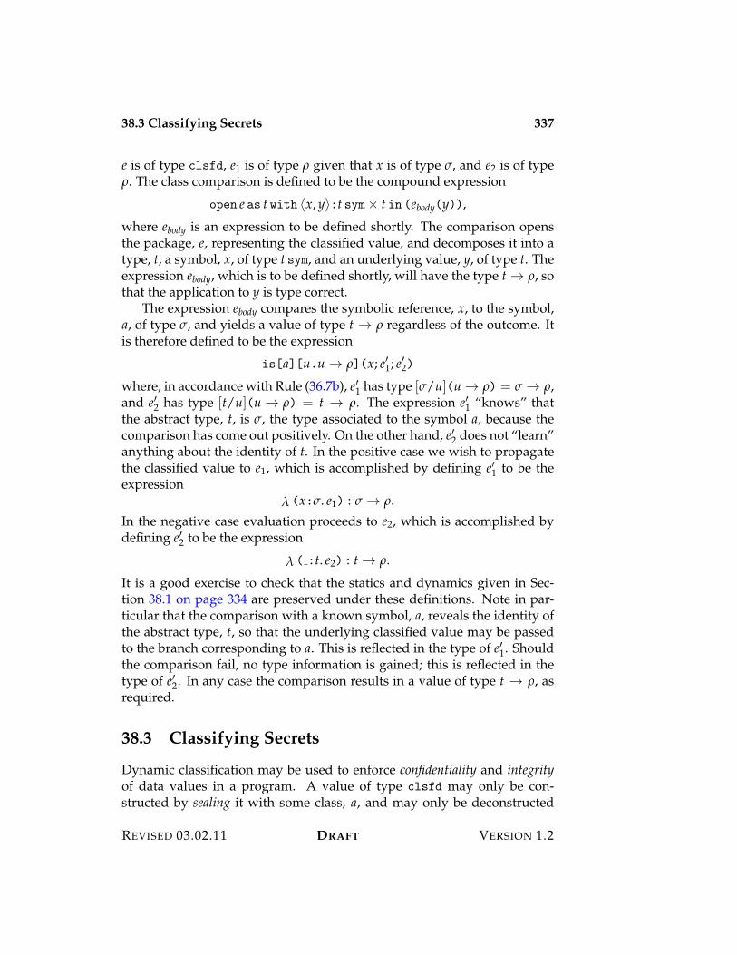
38.3 Classifying Secrets 337
e is of type clsfd, e1 is of type , given that x is of type &, and e2 is of type,. The class comparison is defined to be the compound expression
open e as t with ?x, y@:t sym< t in (ebody(y)),
where ebody is an expression to be defined shortly. The comparison opensthe package, e, representing the classified value, and decomposes it into atype, t, a symbol, x, of type t sym, and an underlying value, y, of type t. Theexpression ebody, which is to be defined shortly, will have the type t 3 ,, sothat the application to y is type correct.
The expression ebody compares the symbolic reference, x, to the symbol,a, of type &, and yields a value of type t 3 , regardless of the outcome. Itis therefore defined to be the expression
is[a][u.u 3 ,](x; e%1; e%2)
where, in accordance with Rule (36.7b), e%1 has type [&/u](u 3 ,) = & 3 ,,and e%2 has type [t/u](u 3 ,) = t 3 ,. The expression e%1 “knows” thatthe abstract type, t, is &, the type associated to the symbol a, because thecomparison has come out positively. On the other hand, e%2 does not “learn”anything about the identity of t. In the positive case we wish to propagatethe classified value to e1, which is accomplished by defining e%1 to be theexpression
! (x:&. e1) : & 3 ,.In the negative case evaluation proceeds to e2, which is accomplished bydefining e%2 to be the expression
! ( :t. e2) : t 3 ,.
It is a good exercise to check that the statics and dynamics given in Sec-tion 38.1 on page 334 are preserved under these definitions. Note in par-ticular that the comparison with a known symbol, a, reveals the identity ofthe abstract type, t, so that the underlying classified value may be passedto the branch corresponding to a. This is reflected in the type of e%1. Shouldthe comparison fail, no type information is gained; this is reflected in thetype of e%2. In any case the comparison results in a value of type t 3 ,, asrequired.
38.3 Classifying Secrets
Dynamic classification may be used to enforce confidentiality and integrityof data values in a program. A value of type clsfd may only be con-structed by sealing it with some class, a, and may only be deconstructed
REVISED 03.02.11 DRAFT VERSION 1.2
338 38.4 Exercises
by a case analysis that includes a branch for a. By controlling which partiesin a multi-party interaction have access to the classifier, a, we may controlhow classified values are created (ensuring their integrity) and how theyare inspected (ensuring their confidentiality). Any party that lacks accessto a cannot decipher a value classified by a, nor may it create a classifiedvalue with this class. Because classes are dynamically generated symbols,they provide an absolute confidentiality guarantee among parties in a com-putation.2
Consider the following simple protocol for controlling the integrity andconfidentiality of data in a program. A fresh symbol, a, is introduced, andwe return a pair of functions of type
(" 3 clsfd)< (clsfd 3 " opt),
called the constructor and destructor functions for that class.
newsym a:" in
? ! (x:". a · x),! (x:clsfd. match x as a · y ; null ow ; just(y)) @.
The first function creates a value classified by a, and the second functionrecovers the instance data of a value classified by a. Outside of the scope ofthe declaration the symbol a is an absolutely unguessable secret.
To enforce the integrity of a value of type ", it is sufficient to ensure thatonly trusted parties have access to the constructor. To enforce the confiden-tiality of a value of type ", it is sufficient to ensure that only trusted partieshave access to the destructor. Ensuring the integrity of a value amounts toassociating an invariant to it that is maintained by the trusted parties thatmay create an instance of that class. Ensuring the confidentiality of a valueamounts to propagating the invariant to parties that may decipher it.
38.4 Exercises
1. Show how to use dynamic classification to implement exceptions.
2Of course, this guarantee is for programs written in conformance with the statics givenhere. If the abstraction imposed by the type system is violated, no guarantees of confiden-tiality can be made.
VERSION 1.2 DRAFT REVISED 03.02.11

Part XIV
Storage Effects

Chapter 39
Modernized Algol
Modernized Algol, or MA, is an imperative, block-structured programminglanguage based on the classic language Algol. MA may be seen as an ex-tension to PCF with a new syntactic sort of commands that act on assignablevariables (or assignables for short) by retrieving and altering their contents.Assignables are introduced by declaring them for use within a specifiedscope; this is the essence of block structure. Commands may be combinedby sequencing, and may be iterated using recursion.
MA maintains a careful separation between pure expressions, whosemeaning does not depend on any assignables, and impure commands, whosemeaning is given in terms of assignables. This ensures that the evaluationorder for expressions is not constrained by the presence of assignables inthe language, and allows for expressions to be manipulated much as inPCF. Commands, on the other hand, have a tightly constrained executionorder, because the execution of one may affect the meaning of another.
A distinctive feature of MA is that it adheres to the stack discipline, whichmeans that assignables are allocated on entry to the scope of their declara-tion, and deallocated on exit, using a conventional stack discipline. Thisavoids the need for more complex forms of storage management, at theexpense of reducing the expressiveness of the language. (Relaxing this re-striction is the subject of Chapter 40.)
39.1 Basic Commands
The syntax of MA distinguishes pure expressions from impure commands.The expressions include those of L{nat"} (as described in Chapter 13),augmented with one additional construct, and the commands are those
342 39.1 Basic Commands
of a simple imperative programming language based on assignment. Thelanguage maintains a sharp distinction between mathematical variables, orjust variables, and assignable variables, or just assignables. Variables are intro-duced by !-abstraction, and are given meaning by substitution. Assignablesare introduced by a declaration, and are given meaning by assignmentand retrieval of their contents, which is, for the time being, restricted tonatural numbers. Expressions evaluate to values, and have no effect onassignables. Commands are executed for their effect on assignables, andalso return a value. Composition of commands not only sequences theirexecution order, but also passes the value returned by the first to the sec-ond before it is executed. The returned value of a command is, for the timebeing, restricted to the natural numbers. (But see Section 39.3 on page 349for the general case.)
The syntax of MA is given by the following grammar, from which wehave omitted repetition of the expression syntax of L{nat"} for the sakeof brevity.
Type " ::= cmd cmd commandExpr e ::= do(m) dom encapsulationCmd m ::= ret(e) ret e return
bnd(e; x.m) bnd x 2 e ; m sequencedcl(e; a.m) dcl a := e inm new assignableget[a] a fetchset[a](e) a := e assign
The expression do(m) consists of the unevaluated command, m, thoughtof as a value of type cmd. The command, ret(e), returns the value of theexpression e without having any effect on the assignables. The commandbnd(e; x.m) evaluates e to an encapulated command, which is then exe-cuted and its returned value is substituted for x prior to executing m. Thecommand dcl(e; a.m) introduces a new assignable, a, for use within thecommand, m, whose initial contents is given by the expression, e. The com-mand get[a] returns the current contents of the assignable, a, and the com-mand set[a](e) changes the contents of the assignable a to the value of e,and returns that value.
39.1.1 Statics
The statics of MA consists of two forms of judgement:
1. Expression typing: ! )$ e : ".
VERSION 1.2 DRAFT REVISED 03.02.11
39.1 Basic Commands 343
2. Command formation: ! )$ m ok.
The context, !, specifies the types of variables, as usual, and the signature,$, consists of a finite set of assignables. These judgements are inductivelydefined by the following rules:
! )$ m ok! )$ do(m) : cmd
(39.1a)
! )$ e : nat! )$ ret(e) ok
(39.1b)
! )$ e : cmd !, x : nat )$ m ok! )$ bnd(e; x.m) ok
(39.1c)
! )$ e : nat ! )$,a m ok
! )$ dcl(e; a.m) ok(39.1d)
! )$,a get[a] ok(39.1e)
! )$,a e : nat! )$,a set[a](e) ok
(39.1f)
Rule (39.1a) is the introductory rule for the type cmd, and Rule (39.1c) is thecorresponding eliminatory form. Rule (39.1d) introduces a new assignablefor use within a specified command. The name, a, of the assignable isbound by the declaration, and hence may be renamed to satisfy the im-plicit constraint that it not already be present in $. Rule (39.1e) states thatthe command to retrieve the contents of an assignable, a, returns a natu-ral number. Rule (39.1f) states that we may assign a natural number to anassignable.
39.1.2 Dynamics
The dynamics of MA is defined in terms of a memory, µ, a finite functionassigning a numeral to each of a finite set of assignables.
The dynamics of expressions consists of these two judgement forms:
1. e val$, stating that e is a value relative to $.
2. e 5$3$
e%, stating that the expression e steps to the expression e%.
REVISED 03.02.11 DRAFT VERSION 1.2
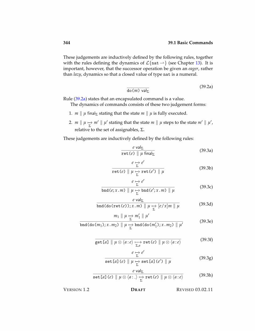
344 39.1 Basic Commands
These judgements are inductively defined by the following rules, togetherwith the rules defining the dynamics of L{nat"} (see Chapter 13). It isimportant, however, that the successor operation be given an eager, ratherthan lazy, dynamics so that a closed value of type nat is a numeral.
do(m) val$(39.2a)
Rule (39.2a) states that an encapsulated command is a value.The dynamics of commands consists of these two judgement forms:
1. m / µ final$ stating that the state m / µ is fully executed.
2. m / µ 5$3$
m% / µ% stating that the state m / µ steps to the state m% / µ%,relative to the set of assignables, $.
These judgements are inductively defined by the following rules:
e val$ret(e) / µ final$
(39.3a)
e 5$3$
e%
ret(e) / µ 5$3$
ret(e%) / µ(39.3b)
e 5$3$
e%
bnd(e; x.m) / µ 5$3$
bnd(e%; x.m) / µ(39.3c)
e val$bnd(do(ret(e)); x.m) / µ 5$3
$[e/x]m / µ (39.3d)
m1 / µ 5$3$
m%1 / µ%
bnd(do(m1); x.m2) / µ 5$3$
bnd(do(m%1); x.m2) / µ% (39.3e)
get[a] / µ E ?a : e@ 5$3$,a
ret(e) / µ E ?a : e@ (39.3f)
e 5$3$
e%
set[a](e) / µ 5$3$
set[a](e%) / µ(39.3g)
e val$set[a](e) / µ E ?a : @ 5$3
$ret(e) / µ E ?a : e@ (39.3h)
VERSION 1.2 DRAFT REVISED 03.02.11
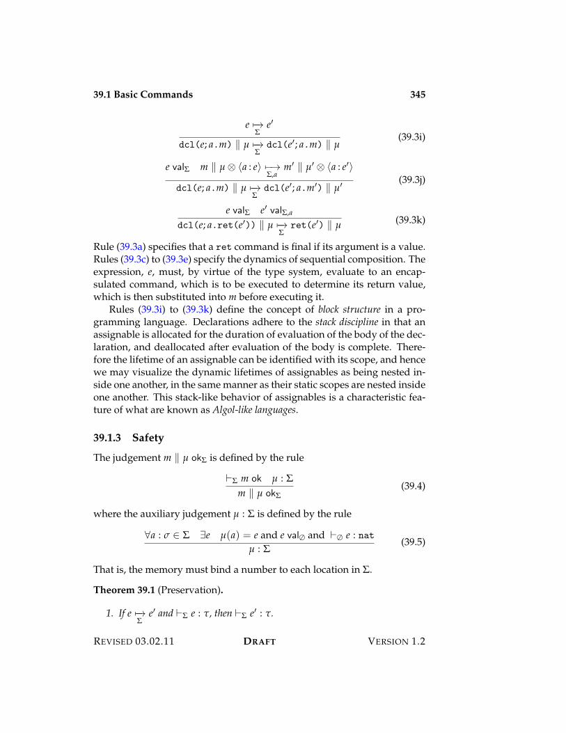
39.1 Basic Commands 345
e 5$3$
e%
dcl(e; a.m) / µ 5$3$
dcl(e%; a.m) / µ(39.3i)
e val$ m / µ E ?a : e@ 5$3$,a
m% / µ% E ?a : e%@
dcl(e; a.m) / µ 5$3$
dcl(e%; a.m%) / µ% (39.3j)
e val$ e% val$,a
dcl(e; a.ret(e%)) / µ 5$3$
ret(e%) / µ (39.3k)
Rule (39.3a) specifies that a ret command is final if its argument is a value.Rules (39.3c) to (39.3e) specify the dynamics of sequential composition. Theexpression, e, must, by virtue of the type system, evaluate to an encap-sulated command, which is to be executed to determine its return value,which is then substituted into m before executing it.
Rules (39.3i) to (39.3k) define the concept of block structure in a pro-gramming language. Declarations adhere to the stack discipline in that anassignable is allocated for the duration of evaluation of the body of the dec-laration, and deallocated after evaluation of the body is complete. There-fore the lifetime of an assignable can be identified with its scope, and hencewe may visualize the dynamic lifetimes of assignables as being nested in-side one another, in the same manner as their static scopes are nested insideone another. This stack-like behavior of assignables is a characteristic fea-ture of what are known as Algol-like languages.
39.1.3 Safety
The judgement m / µ ok$ is defined by the rule
)$ m ok µ : $m / µ ok$
(39.4)
where the auxiliary judgement µ : $ is defined by the rule
&a : & + $ 'e µ(a) = e and e val# and )# e : natµ : $
(39.5)
That is, the memory must bind a number to each location in $.
Theorem 39.1 (Preservation).
1. If e 5$3$
e% and )$ e : ", then )$ e% : ".
REVISED 03.02.11 DRAFT VERSION 1.2
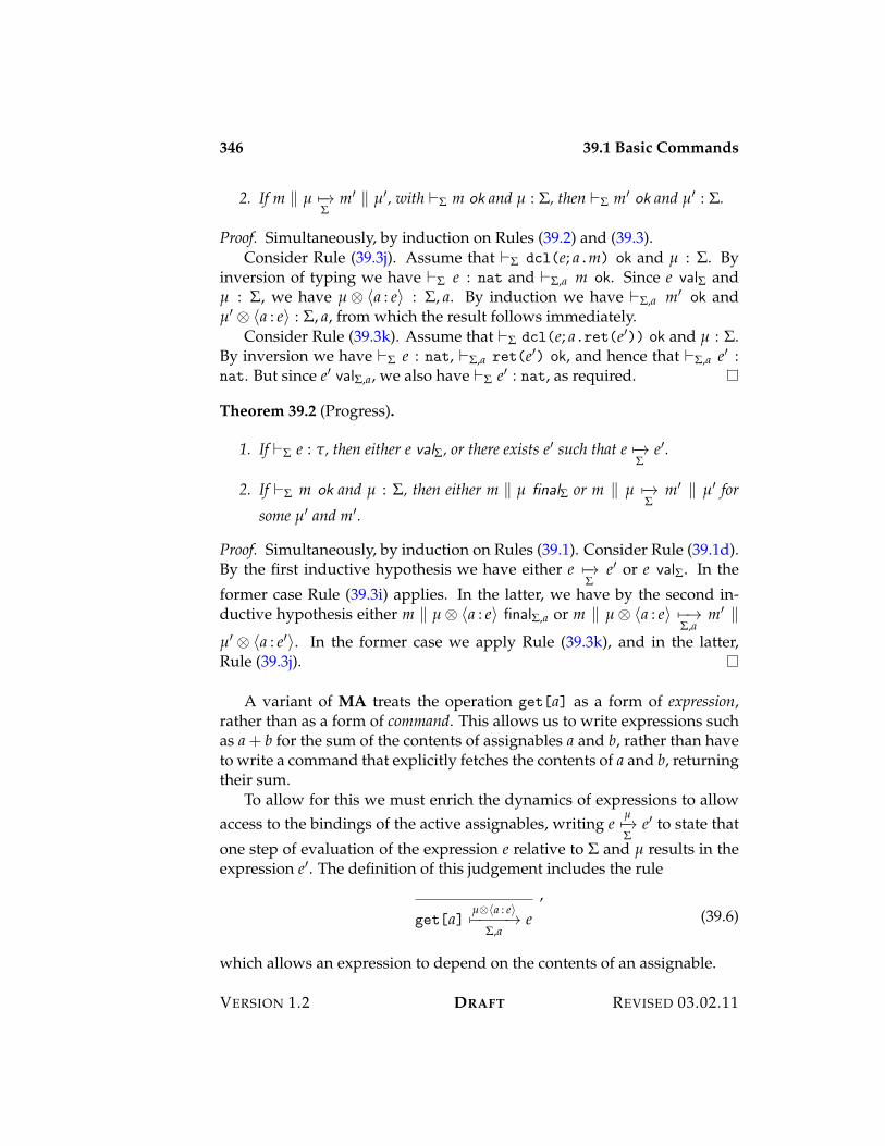
346 39.1 Basic Commands
2. If m / µ 5$3$
m% / µ%, with )$ m ok and µ : $, then )$ m% ok and µ% : $.
Proof. Simultaneously, by induction on Rules (39.2) and (39.3).Consider Rule (39.3j). Assume that )$ dcl(e; a.m) ok and µ : $. By
inversion of typing we have )$ e : nat and )$,a m ok. Since e val$ andµ : $, we have µ E ?a : e@ : $, a. By induction we have )$,a m% ok andµ% E ?a : e@ : $, a, from which the result follows immediately.
Consider Rule (39.3k). Assume that )$ dcl(e; a.ret(e%)) ok and µ : $.By inversion we have )$ e : nat, )$,a ret(e%) ok, and hence that )$,a e% :nat. But since e% val$,a, we also have )$ e% : nat, as required.
Theorem 39.2 (Progress).
1. If )$ e : ", then either e val$, or there exists e% such that e 5$3$
e%.
2. If )$ m ok and µ : $, then either m / µ final$ or m / µ 5$3$
m% / µ% for
some µ% and m%.
Proof. Simultaneously, by induction on Rules (39.1). Consider Rule (39.1d).By the first inductive hypothesis we have either e 5$3
$e% or e val$. In the
former case Rule (39.3i) applies. In the latter, we have by the second in-ductive hypothesis either m / µ E ?a : e@ final$,a or m / µ E ?a : e@ 5$3
$,am% /
µ% E ?a : e%@. In the former case we apply Rule (39.3k), and in the latter,Rule (39.3j).
A variant of MA treats the operation get[a] as a form of expression,rather than as a form of command. This allows us to write expressions suchas a + b for the sum of the contents of assignables a and b, rather than haveto write a command that explicitly fetches the contents of a and b, returningtheir sum.
To allow for this we must enrich the dynamics of expressions to allowaccess to the bindings of the active assignables, writing e
µ5$3$
e% to state thatone step of evaluation of the expression e relative to $ and µ results in theexpression e%. The definition of this judgement includes the rule
get[a]µE?a : e@5$$$$3
$,ae
,(39.6)
which allows an expression to depend on the contents of an assignable.
VERSION 1.2 DRAFT REVISED 03.02.11
39.2 Some Programming Idioms 347
39.2 Some Programming Idioms
The language MA is designed to expose the elegant interplay between theexecution of an expression for its value and the execution of a commandfor its effect on assignables. In this section we show how to derive severalstandard idioms of imperative programming in MA.
We define the sequential composition of commands, written {x 2 m1 ; m2},to stand for the command bnd x2 do (m1) ; m2. This generalizes to an n-aryform by defining
{x1 2 m1 ; . . . xn$1 2 mn$1 ; mn},
to stand for the iterated composition
{x1 2 m1 ; . . . {xn$1 2 mn$1 ; mn}}.
We sometimes write just {m1 ; m2} for the composition { 2 m1 ; m2} inwhich the returned value from m1 is ignored; this generalizes in the ob-vious way to an n-ary form.
A related idiom, the command run e, executes an encapsulated com-mand and returns its result; it for bnd x 2 e ; ret x.
The conditional command, if (m)m1 elsem2, executes either m1 or m2according to whether the result of executing m is zero or not:
{x 2 m ; run (ifz x {z; dom1 | s( ); dom2})}.
The returned value of the conditional is the value returned by the selectedcommand.
The while loop command, while (m1)m2, repeatedly executes the com-mand m2 while the command m1 yields a non-zero number. It is defined asfollows:
run (fix loop:cmd is do(if (m1) {ret z} else {m2 ; run loop})).
This commands runs the self-referential encapsulated command that, whenexecuted, first executes m1, branching on the result. If the result is zero, theloop returns zero (arbitrarily). If the result is non-zero, the command m2 isexecuted and the loop is repeated.
A procedure is a function of type " " cmd that takes an argument of sometype, ", and yields an unexecuted command as result. A procedure call is thecomposition of a function application with the activation of the resulting
REVISED 03.02.11 DRAFT VERSION 1.2
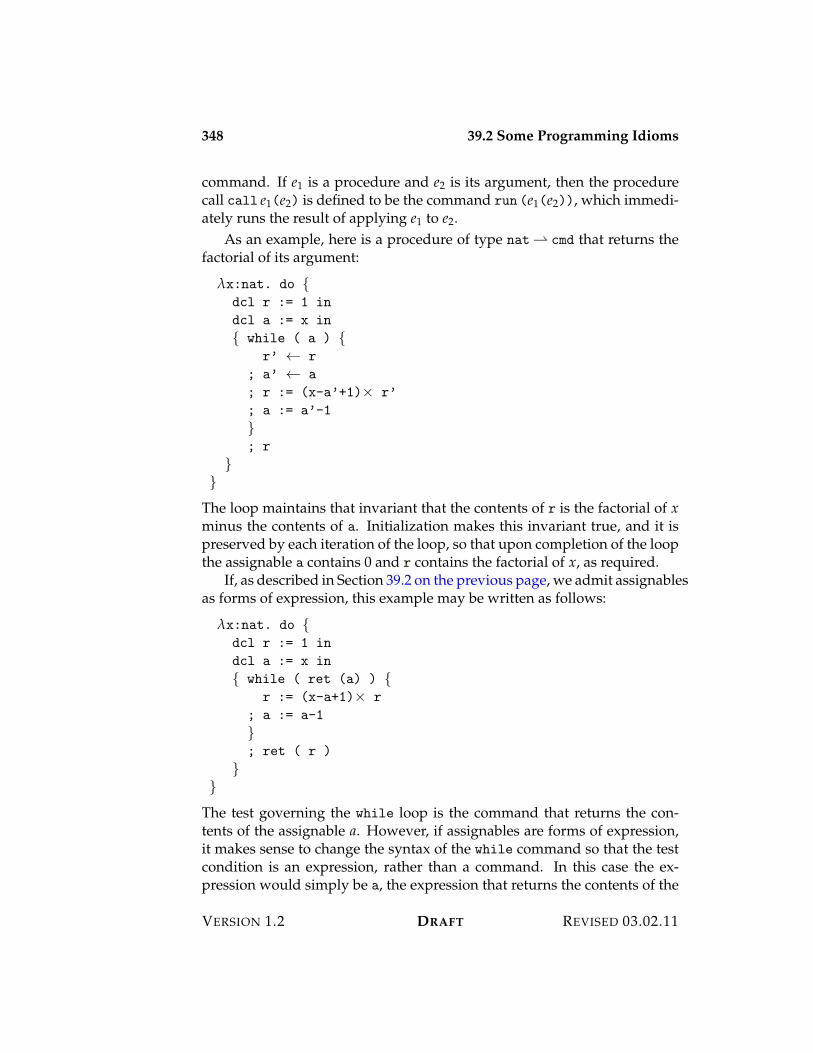
348 39.2 Some Programming Idioms
command. If e1 is a procedure and e2 is its argument, then the procedurecall call e1(e2) is defined to be the command run (e1(e2)), which immedi-ately runs the result of applying e1 to e2.
As an example, here is a procedure of type nat" cmd that returns thefactorial of its argument:
!x:nat. do {dcl r := 1 in
dcl a := x in
{ while ( a ) {r’ 2 r
; a’ 2 a
; r := (x-a’+1)< r’
; a := a’-1
}; r
}}
The loop maintains that invariant that the contents of r is the factorial of xminus the contents of a. Initialization makes this invariant true, and it ispreserved by each iteration of the loop, so that upon completion of the loopthe assignable a contains 0 and r contains the factorial of x, as required.
If, as described in Section 39.2 on the previous page, we admit assignablesas forms of expression, this example may be written as follows:
!x:nat. do {dcl r := 1 in
dcl a := x in
{ while ( ret (a) ) {r := (x-a+1)< r
; a := a-1
}; ret ( r )
}}
The test governing the while loop is the command that returns the con-tents of the assignable a. However, if assignables are forms of expression,it makes sense to change the syntax of the while command so that the testcondition is an expression, rather than a command. In this case the ex-pression would simply be a, the expression that returns the contents of the
VERSION 1.2 DRAFT REVISED 03.02.11
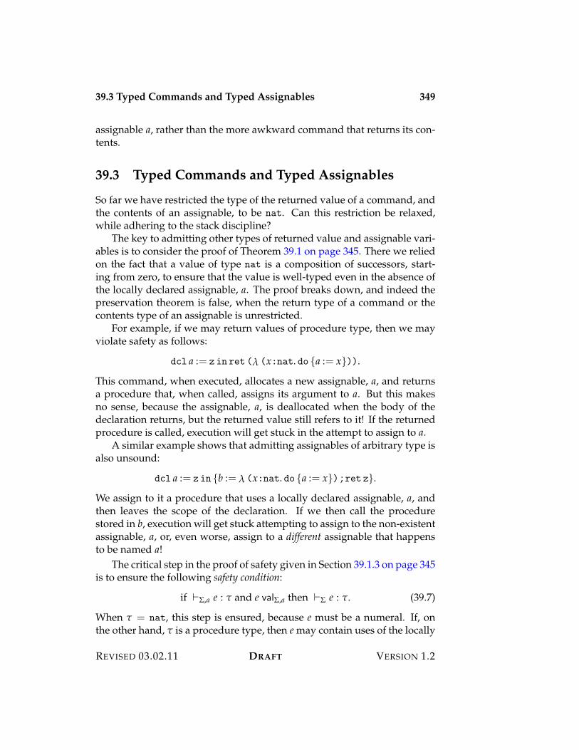
39.3 Typed Commands and Typed Assignables 349
assignable a, rather than the more awkward command that returns its con-tents.
39.3 Typed Commands and Typed Assignables
So far we have restricted the type of the returned value of a command, andthe contents of an assignable, to be nat. Can this restriction be relaxed,while adhering to the stack discipline?
The key to admitting other types of returned value and assignable vari-ables is to consider the proof of Theorem 39.1 on page 345. There we reliedon the fact that a value of type nat is a composition of successors, start-ing from zero, to ensure that the value is well-typed even in the absence ofthe locally declared assignable, a. The proof breaks down, and indeed thepreservation theorem is false, when the return type of a command or thecontents type of an assignable is unrestricted.
For example, if we may return values of procedure type, then we mayviolate safety as follows:
dcl a := z in ret (! (x:nat. do {a := x})).
This command, when executed, allocates a new assignable, a, and returnsa procedure that, when called, assigns its argument to a. But this makesno sense, because the assignable, a, is deallocated when the body of thedeclaration returns, but the returned value still refers to it! If the returnedprocedure is called, execution will get stuck in the attempt to assign to a.
A similar example shows that admitting assignables of arbitrary type isalso unsound:
dcl a := z in {b := ! (x:nat. do {a := x}) ; ret z}.
We assign to it a procedure that uses a locally declared assignable, a, andthen leaves the scope of the declaration. If we then call the procedurestored in b, execution will get stuck attempting to assign to the non-existentassignable, a, or, even worse, assign to a different assignable that happensto be named a!
The critical step in the proof of safety given in Section 39.1.3 on page 345is to ensure the following safety condition:
if )$,a e : " and e val$,a then )$ e : ". (39.7)
When " = nat, this step is ensured, because e must be a numeral. If, onthe other hand, " is a procedure type, then e may contain uses of the locally
REVISED 03.02.11 DRAFT VERSION 1.2
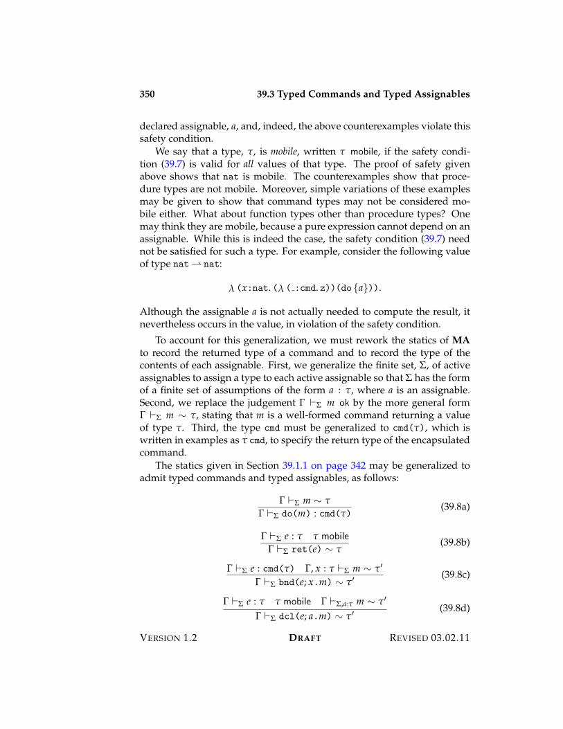
350 39.3 Typed Commands and Typed Assignables
declared assignable, a, and, indeed, the above counterexamples violate thissafety condition.
We say that a type, ", is mobile, written " mobile, if the safety condi-tion (39.7) is valid for all values of that type. The proof of safety givenabove shows that nat is mobile. The counterexamples show that proce-dure types are not mobile. Moreover, simple variations of these examplesmay be given to show that command types may not be considered mo-bile either. What about function types other than procedure types? Onemay think they are mobile, because a pure expression cannot depend on anassignable. While this is indeed the case, the safety condition (39.7) neednot be satisfied for such a type. For example, consider the following valueof type nat" nat:
! (x:nat. (! ( :cmd. z))(do {a})).
Although the assignable a is not actually needed to compute the result, itnevertheless occurs in the value, in violation of the safety condition.
To account for this generalization, we must rework the statics of MAto record the returned type of a command and to record the type of thecontents of each assignable. First, we generalize the finite set, $, of activeassignables to assign a type to each active assignable so that $ has the formof a finite set of assumptions of the form a : ", where a is an assignable.Second, we replace the judgement ! )$ m ok by the more general form! )$ m I ", stating that m is a well-formed command returning a valueof type ". Third, the type cmd must be generalized to cmd("), which iswritten in examples as " cmd, to specify the return type of the encapsulatedcommand.
The statics given in Section 39.1.1 on page 342 may be generalized toadmit typed commands and typed assignables, as follows:
! )$ m I "! )$ do(m) : cmd(")
(39.8a)
! )$ e : " " mobile! )$ ret(e) I "
(39.8b)
! )$ e : cmd(") !, x : " )$ m I "%
! )$ bnd(e; x.m) I "% (39.8c)
! )$ e : " " mobile ! )$,a:" m I "%
! )$ dcl(e; a.m) I "% (39.8d)
VERSION 1.2 DRAFT REVISED 03.02.11
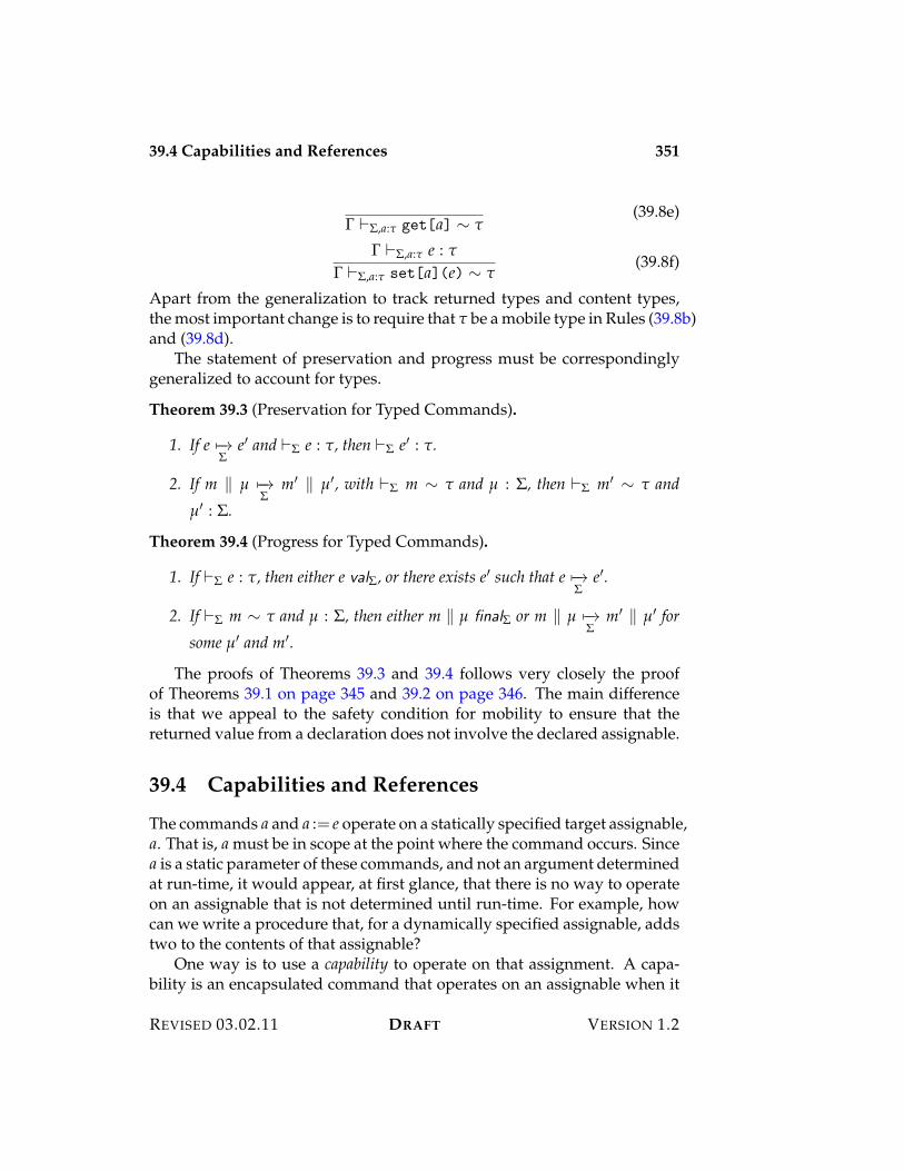
39.4 Capabilities and References 351
! )$,a:" get[a] I "(39.8e)
! )$,a:" e : "
! )$,a:" set[a](e) I "(39.8f)
Apart from the generalization to track returned types and content types,the most important change is to require that " be a mobile type in Rules (39.8b)and (39.8d).
The statement of preservation and progress must be correspondinglygeneralized to account for types.
Theorem 39.3 (Preservation for Typed Commands).
1. If e 5$3$
e% and )$ e : ", then )$ e% : ".
2. If m / µ 5$3$
m% / µ%, with )$ m I " and µ : $, then )$ m% I " and
µ% : $.
Theorem 39.4 (Progress for Typed Commands).
1. If )$ e : ", then either e val$, or there exists e% such that e 5$3$
e%.
2. If )$ m I " and µ : $, then either m / µ final$ or m / µ 5$3$
m% / µ% for
some µ% and m%.
The proofs of Theorems 39.3 and 39.4 follows very closely the proofof Theorems 39.1 on page 345 and 39.2 on page 346. The main differenceis that we appeal to the safety condition for mobility to ensure that thereturned value from a declaration does not involve the declared assignable.
39.4 Capabilities and References
The commands a and a := e operate on a statically specified target assignable,a. That is, a must be in scope at the point where the command occurs. Sincea is a static parameter of these commands, and not an argument determinedat run-time, it would appear, at first glance, that there is no way to operateon an assignable that is not determined until run-time. For example, howcan we write a procedure that, for a dynamically specified assignable, addstwo to the contents of that assignable?
One way is to use a capability to operate on that assignment. A capa-bility is an encapsulated command that operates on an assignable when it
REVISED 03.02.11 DRAFT VERSION 1.2
352 39.4 Capabilities and References
is activated. The get capability, or getter, for an assignable a of type " is thecommand do {a} of type " cmd that, when executed, returns the contentsof a. The set capability, or setter, for a is the procedure ! (x:". do {a := x})that, when applied, assigns its argument to a. Since capabilities are pairs ofprocedures, they are not mobile.
A general double-increment procedure that operates on any assignable,regardless of whether it is in scope, may be programmed as follows:
! (get:nat cmd. ! (set:nat" nat cmd. do {x 2 get ; set(s(s(x)))})).
The procedure is to be called with a getter and a setter for the same assignable.When executed, it invokes the getter to obtain the contents of that assignable,and then invokes the setter to assign its contents to be two more than thevalue it contained.
Although it is natural to consider the get and set capabilities for anassignable as a pair, it can be useful to separate them to provide limitedaccess to an assignable in a particular context. If only the get capability ispassed to a procedure, then its result may depend on the contents of theunderlying assignable, but may not alter it. Similarly, if only the set capa-bility is passed, then it may alter the contents of the underlying assignable,but cannot access its current contents. It is also useful to consider otherforms of capability than simple getters and setters. For example, one coulddefine an increment and a decrement capability for an assignable, and passone or both to a procedure to limit how it may influence the value of thatassignable. The possibilities are endless.
Returning to the double-increment example, the type does not constrainthe caller to provide get and set capabilities that act on the same assignable.One way to ensure this is to introduce a name, or reference, to an assignableas a form of value. A reference may be thought of as a token that providesaccess to the get and set capabilities of an assignable. Moreover, two ref-erences may be tested for equality, so that one may determine at run-timewhether they refer to the same underlying assignable.1
A reference is a value of type ref("), where " is the type of the con-tents of the assignable to which it refers. A (closed) value of reference typeis the name of an assignable thought of as a form of expression. Possess-ing a reference allows one to perform either a get or a set operation on theunderlying assignable. (One may also consider read-only or write-only ref-erences, or more complex capabilities for assignables, in a similar manner.)
1This can also be achieved using capabilities by using the setter for one to modify theassignable and using the getter for the other to determine whether it changed.
VERSION 1.2 DRAFT REVISED 03.02.11
39.4 Capabilities and References 353
This suggests the following syntax for references:
Type " ::= ref(") " ref assignableExpr e ::= ref[a] & a referenceCmd m ::= getref(e) @ e contents
setref(e1; e2) e1 := e2 update
The statics of references is given by the following rules:
! )$,a:" ref[a] : ref(")(39.9a)
! )$ e : ref(")! )$ getref(e) I "
(39.9b)
! )$ e1 : ref(") ! )$ e2 : "! )$ setref(e1; e2) I "
(39.9c)
Rule (39.9a) specifies that the name of any active assignable is an expressionof type ref(").
The dynamics is defined to defer to the corresponding operation on theassignable to which a reference refers.
ref[a] val$,a(39.10a)
e 5$3$
e%
getref(e) / µ 5$3$
getref(e%) / µ(39.10b)
getref(ref[a]) / µ 5$3$
get[a] / µ(39.10c)
e1 5$3$
e%1
setref(e1; e2) / µ 5$3$
setref(e%1; e2) / µ(39.10d)
setref(ref[a]; e) / µ 5$3$
set[a](e) / µ(39.10e)
A reference to an assignable is a value. The getref and setref operationson references defer to the corresponding operations on assignables once thereference has been determined.
REVISED 03.02.11 DRAFT VERSION 1.2
354 39.4 Capabilities and References
Suprisingly, the addition of references to assignables does not violatethe stack discipline, so long as reference types are deemed immobile. Thisensures that a reference can never escape the scope of the assignable towhich it refers, which is essential to maintaining safety. We leave to thereader the task of proving safety for the extension of MA with referencetypes.
As an example of programming with references, the double incrementprocedure given earlier can be coded using references, rather than capabil-ities, as follows:
! (r:nat ref. do {x 2 @ r ; r := s(s(x))}).
Since the argument is a reference to an assignable, rather than a get andset capability, it is assured that the body of the procedure acts on a singleassignable when performing the get and set operations on the reference.
References and capabilities allow assignables to be treated as valuesthat can be passed as arguments to procedures. This allows us to writeprograms, such as the double increment procedure, that act on assignablesthat are not in scope within the body of the procedure. Such expressivepower, however, comes at a price: we must carefully consider whether tworeferences refer to the same assignable or not. This phenomenon is calledaliasing; it greatly complicates reasoning about program correctness.
Consider, for example, the problem of writing a procedure that, whengiven two references, x and y, adds twice the contents of y to the contentsof x. One way to write this code creates no complications:
! (x:nat ref. ! (y:nat ref. do {x% 2 @ x ; y% 2 @ y ; x := x% + y% + y%})).
Even if x and y refer to the same assignable, the effect will be to set the con-tents of the assignable referenced by x to twice the contents of the assignablereferenced by y.
But now consider the following apparently equivalent implementationof the “same” procedure:
! (x:nat ref. ! (y:nat ref. do {x += y ; x += y})),
where x += y is the command
{x% 2 @ x ; y% 2 @ y ; x := x% + y%}
that adds the contents of y to the contents of x. The second implementationworks properly provided that x and y do not refer to the same assignable.
VERSION 1.2 DRAFT REVISED 03.02.11
39.5 Exercises 355
For if they are aliases in that they both refer to the same assignable, a, withcontents n0, the result is that a is to set 4< n0, instead of the intended 3< n0.
In this case it is entirely obvious how to avoid the problem: use the firstimplementation, rather than the second. But the difficulty is not in fixingthe problem once it has been uncovered, but rather noticing the problem inthe first place! Wherever references (or capabilities) are used, the problemsof interference lurk. Avoiding them requires very careful consideration ofall possible aliasing relationships among all of the references in play at agiven point of a computation. The problem is that the number of possiblealiasing relationships among n references grows at least quadratically in n(we must consider all possible pairings) and can even be worse when moresubtle relationships among three or more variables must be considered.Aliasing is a prime source of errors in imperative programs, and remains astrong argument against using imperative methods whenever possible.
39.5 Exercises
REVISED 03.02.11 DRAFT VERSION 1.2

356 39.5 Exercises
VERSION 1.2 DRAFT REVISED 03.02.11
Chapter 40
Mutable Data Structures
In Chapter 39 we considered an imperative programming language thatadheres to the stack discipline in that assignables are allocated and de-allocated on a last-in, first-out basis. To ensure this we restricted the typesof return values from a command, the types of contents of assignables, to bemobile types, ones whose values cannot depend on the stack of assignables.Function and command types are not mobile, nor are reference types, be-cause these types may classify values that refer to an assignable.
A major use of references, however, is to implement mutable data struc-tures whose structure may be changed at execution time. The classic ex-ample is a linked list in which the tail of any initial segment of the list maybe changed to refer to another list. Crucially, any such alteration is sharedamong all uses of that list. (This behavior is in contrast to an immutablelist, which can never change once created.) The usual way to implement alinked list is to specify that the tail of a list is not another list, but rather areference to an assignable containing the tail of the list. The list structure isaltered by setting the target assignable of the reference.
For this strategy to make sense, references must be mobile, and hencethat assignables have indefinite extent—they must persist beyond the scopeof their declaration. Assignables with indefinite extent are said to be scope-free, or simply free. In this chapter we consider a variation of ModernizedAlgol in which all assignables are free, and hence all types are mobile. Thedynamics of this variation of Modernized Algol is significantly differentfrom that given in Chapter 39 in that assignables are heap-allocated, ratherthan stack-allocated.
We also consider a further variation in which the distinction betweencommands and expressions is eliminated. This facilitates the use of benign
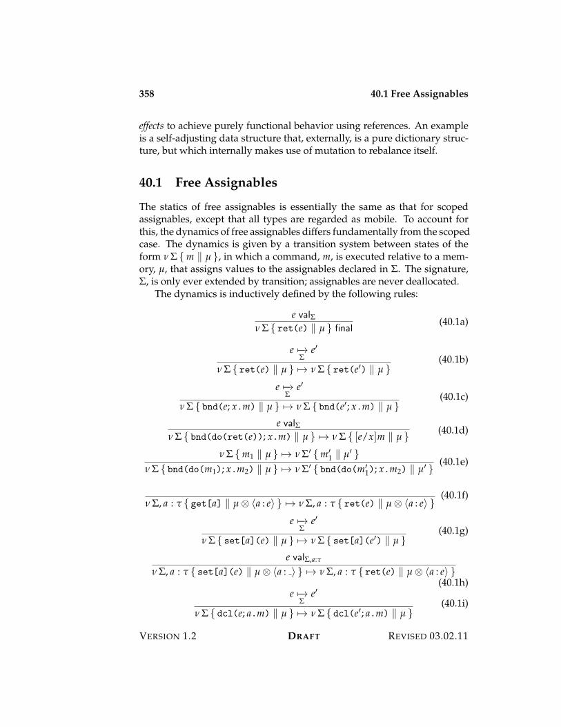
358 40.1 Free Assignables
effects to achieve purely functional behavior using references. An exampleis a self-adjusting data structure that, externally, is a pure dictionary struc-ture, but which internally makes use of mutation to rebalance itself.
40.1 Free Assignables
The statics of free assignables is essentially the same as that for scopedassignables, except that all types are regarded as mobile. To account forthis, the dynamics of free assignables differs fundamentally from the scopedcase. The dynamics is given by a transition system between states of theform 0 $ {m / µ }, in which a command, m, is executed relative to a mem-ory, µ, that assigns values to the assignables declared in $. The signature,$, is only ever extended by transition; assignables are never deallocated.
The dynamics is inductively defined by the following rules:
e val$0 $ { ret(e) / µ } final
(40.1a)
e 5$3$
e%
0 $ { ret(e) / µ } 53 0 $ { ret(e%) / µ }(40.1b)
e 5$3$
e%
0 $ { bnd(e; x.m) / µ } 53 0 $ { bnd(e%; x.m) / µ }(40.1c)
e val$0 $ { bnd(do(ret(e)); x.m) / µ } 53 0 $ { [e/x]m / µ } (40.1d)
0 $ {m1 / µ } 53 0 $% {m%1 / µ% }
0 $ { bnd(do(m1); x.m2) / µ } 53 0 $% { bnd(do(m%1); x.m2) / µ% }
(40.1e)
0 $, a : " { get[a] / µ E ?a : e@ } 53 0 $, a : " { ret(e) / µ E ?a : e@ }(40.1f)
e 5$3$
e%
0 $ { set[a](e) / µ } 53 0 $ { set[a](e%) / µ }(40.1g)
e val$,a:"
0 $, a : " { set[a](e) / µ E ?a : @ } 53 0 $, a : " { ret(e) / µ E ?a : e@ }(40.1h)
e 5$3$
e%
0 $ { dcl(e; a.m) / µ } 53 0 $ { dcl(e%; a.m) / µ }(40.1i)
VERSION 1.2 DRAFT REVISED 03.02.11
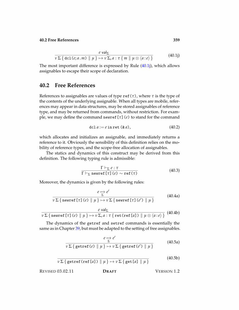
40.2 Free References 359
e val$0 $ { dcl(e; a.m) / µ } 53 0 $, a : " {m / µ E ?a : e@ } (40.1j)
The most important difference is expressed by Rule (40.1j), which allowsassignables to escape their scope of declaration.
40.2 Free References
References to assignables are values of type ref("), where " is the type ofthe contents of the underlying assignable. When all types are mobile, refer-ences may appear in data structures, may be stored assignables of referencetype, and may be returned from commands, without restriction. For exam-ple, we may define the command newref["](e) to stand for the command
dcl a := e in ret (& a), (40.2)
which allocates and initializes an assignable, and immediately returns areference to it. Obviously the sensibility of this definition relies on the mo-bility of reference types, and the scope-free allocation of assignables.
The statics and dynamics of this construct may be derived from thisdefinition. The following typing rule is admissible:
! )$ e : "! )$ newref["](e) I ref(")
(40.3)
Moreover, the dynamics is given by the following rules:
e 5$3$
e%
0 $ { newref["](e) / µ } 53 0 $ { newref["](e%) / µ }(40.4a)
e val$0 $ { newref["](e) / µ } 53 0 $, a : " { ret(ref[a]) / µ E ?a : e@ } (40.4b)
The dynamics of the getref and setref commands is essentially thesame as in Chapter 39, but must be adapted to the setting of free assignables.
e 5$3$
e%
0 $ { getref(e) / µ } 53 0 $ { getref(e%) / µ }(40.5a)
0 $ { getref(ref[a]) / µ } 53 0 $ { get[a] / µ }(40.5b)
REVISED 03.02.11 DRAFT VERSION 1.2
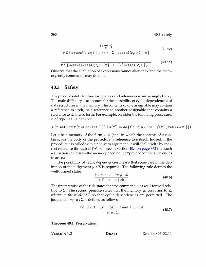
360 40.3 Safety
e1 5$3$
e%1
0 $ { setref(e1; e2) / µ } 53 0 $ { setref(e%1; e2) / µ }(40.5c)
0 $ { setref(ref[a]; e2) / µ } 53 0 $ { set[a](e2) / µ }(40.5d)
Observe that the evaluation of expressions cannot alter or extend the mem-ory, only commands may do this.
40.3 Safety
The proof of safety for free assignables and references is surprisingly tricky.The main difficulty is to account for the possibility of cyclic dependencies ofdata structures in the memory. The contents of one assignable may containa reference to itself, or a reference to another assignable that contains areference to it, and so forth. For example, consider the following procedure,e, of type nat 3 nat cmd:
! (x:nat. ifz x {z; do {ret (1)} | s(x%); do { f 2 a ; y 2 call f(x%) ; ret (x 1 y)}}).
Let µ be a memory of the form µ% E ?a : e@ in which the contents of a con-tains, via the body of the procedure, a reference to a itself. Indeed, if theprocedure e is called with a non-zero argument, it will “call itself” by indi-rect reference through a! (We will see in Section 40.4 on page 362 that sucha situation can arise—the memory need not be “preloaded” for such cyclesto arise.)
The possibility of cyclic dependencies means that some care in the def-inition of the judgement µ : $ is required. The following rule defines thewell-formed states:
)$ m I " )$ µ : $0 $ {m / µ } ok
(40.6)
The first premise of the rule states that the command m is well-formed rela-tive to $. The second premise states that the memory, µ, conforms to $,relative to the whole of $ so that cyclic dependencies are permitted. Thejudgement )$% µ : $ is defined as follows:
&a : & + $ 'e µ(a) = e and )$% e : &
)$% µ : $(40.7)
Theorem 40.1 (Preservation).
VERSION 1.2 DRAFT REVISED 03.02.11
40.3 Safety 361
1. If )$ e : " and e 5$3$
e%, then )$ e% : ".
2. If 0 $ {m / µ } ok and 0 $ {m / µ } 53 0 $% {m% / µ% }, then 0 $% {m% / µ% } ok.
Proof. Simultaneously, by induction on transition. We prove the followingstronger form of the second statement:
If 0 $ {m / µ } 53 0 $% {m% / µ% }, where )$ m I ", )$ µ : $,then $% extends $, and )$% m% I ", and )$% µ% : $%.
Consider, for example, the transition
0 $ { dcl(e; a.m) / µ } 53 0 $, a : & {m / µ E ?a : e@ }
where e val$. By assumption and inversion of Rule (39.8d) we have & suchthat )$ e : &, )$,a:& m I ", and )$ µ : $. But since extension of $ with afresh assignable does not affect typing, we also have )$,a:& µ : $ and )$,a:&e : &, from which it follows by Rule (40.7) that )$,a:& µ E ?a : e@ : $, a : &.
The other cases follow a similar pattern, and are left as an exercise forthe reader.
Theorem 40.2 (Progress).
1. If )$ e : ", then either e val$ or there exists e% such that e 5$3$
e%.
2. If 0 $ {m / µ } ok then either 0 $ {m / µ } final or 0 $ {m / µ } 53 0 $% {m% / µ% }for some $%, µ%, and m%.
Proof. Simultaneously, by induction on typing. For the second statementwe prove the stronger form
If )$ m I " and )$ µ : $, then either 0 $ {m / µ } final, or0 $ {m / µ } 53 0 $% {m% / µ% } for some $%, µ%, and m%.
Consider, for example, the typing rule
! )$ e : & ! )$,a:& m I "
! )$ dcl(e; a.m) I "
We have by the first inductive hypothesis that either e val$ or e 5$3$
e% for
some e%. In the latter case we have by Rule (40.1i)
0 $ { dcl(e; a.m) / µ } 53 0 $ { dcl(e%; a.m) / µ }.
REVISED 03.02.11 DRAFT VERSION 1.2
362 40.4 Integrating Commands and Expressions
In the former case we have by Rule (40.1j) that
0 $ { dcl(e; a.m) / µ } 53 0 $, a : & {m / µ E ?a : e@ }.
As another example, consider the typing rule
! )$,a:" get[a] I "
By assumption )$,a:" µ : $, a : ", and hence there exists e val$,a:" such thatµ = µ% E ?a : e@ and )$,a:" e : ". By Rule (40.1f)
0 $, a : " { get[a] / µ% E ?a : e@ } 53 0 $, a : " { ret(e) / µ% E ?a : e@ },
as required. The other cases are handled similarly.
40.4 Integrating Commands and Expressions
The modal formulation of free assignables maintains the separation betweenexpressions and commands inherited from MA. An important variation onthis design eliminates this distinction, allowing expressions to have bothvalue and effect. This is called the integral formulation of free assignables;it has advantages and disadvantages compared to the modal formulation.
The statics of the integral formulation is obtained by consolidating ex-pressions and commands, dropping the return command since it serves nopurpose. The following rules are illustrative:
! )$ e : "! )$ do(e) : cmd(")
(40.8a)
! )$ e1 : cmd("1) !, x : "1 )$ e2 : "2! )$ bnd(e1; x.e2) : "2
(40.8b)
! )$ e1 : "1 ! )$,a:"1 e2 : "2
! )$ dcl(e1; a.e2) : "2(40.8c)
! )$,a:" get[a] : "(40.8d)
! )$,a:" e : "
! )$,a:" set[a](e) : "(40.8e)
VERSION 1.2 DRAFT REVISED 03.02.11
40.4 Integrating Commands and Expressions 363
The dynamics of the integral formulation of mutation is defined as atransition system between states of the form 0 $ { e / µ }, where e is an ex-pression involving the assignables declared in $, and µ is a memory pro-viding values for each of these assignables. It is a straightforward exer-cise to reformulate Rules (40.1) to eliminate the mode distinction betweencommands and expressions. Rules (40.5) may similarly be adapted to theintegral setting.
The modal and integral formulations of references have complemen-tary strengths and weaknesses. The chief virtue of the modal formulation isthat the use of assignment is confined to commands, leaving expressions aspure computations. One consequence is that typing judgements for expres-sions retain their force even in the presence of references to free assignables,so that the type unit" unit contains only the identity and the divergentfunctions, and the type nat" nat consists solely of partial functions onthe natural numbers. By contrast the integral formulation enjoys none ofthese properties. Any expression may alter or allocate new assignables,and the semantics of typing assertions is therefore significantly weakenedcompared to the modal formulation. In particular, the type unit" unit
contains infinitely many distinct functions, and the type nat" nat con-tains procedures that in no way represent partial functions because theyretain state across calls.
While the modal separation of pure expressions from impure commandsmay seem like an unalloyed good, the situation is actually more complex.The central problem is that the modal formulation inhibits the use of effectsto implement purely functional behavior. For example, a self-adjustingtree, such as a splay tree, uses in-place mutation to provide an efficientimplementation of what is otherwise a purely functional dictionary struc-ture mapping keys to values. This is an example of a benign effect, one thatdoes not affect the behavior, but only the efficiency, of the implementation.
Many other examples arise in practice. For example, suppose that wewish to instrument an otherwise pure functional program with code to col-lect execution statistics for profiling. In the integral setting it is a simplematter to allocate free assignables that contain profiling information col-lected by assignments that update their contents at critical points in theprogram. In the modal setting, however, we must globally restructure theprogram to transform it from a pure expression to an impure command.Another example is provided by the technique of backpatching for imple-menting recursion using a free assignable, which we now describe in moredetail.
REVISED 03.02.11 DRAFT VERSION 1.2
364 40.4 Integrating Commands and Expressions
In the integral formulation we may implement the factorial functionusing backpatching as follows:
dcl a := !n:nat.0 in
{ f 2 !n:nat.ifz(n, 1, n’.n * a(n’))
; 2 a := f
; f
}
wherein we have used the concrete syntax for commands introduced inChapter 39. Observe that the assignable a is used as an expression standingfor its contents (that is, it stands for the abstract syntax get[a]).
This expression returns a function of type nat" nat that is obtainedby (a) allocating a free assignable initialized arbitrarily (and immaterially)with a function of this type, (b) defining a !-abstraction in which each “re-cursive call” consists of retrieving and applying the function stored in thatassignable, (c) assigning this function to the assignable, and (d) returningthat function. The result is a value of function type that uses an assignable“under the hood” in a manner not visible to its clients.
In contrast the modal formulation forces us to make explicit the relianceon private state.
dcl a := !n:nat.do{ret 0} in
{ f 2 ret (! n:nat. ...)
; 2 a := f
; ret f
}
where the elided procedure body is as follows:
ifz(n,do{ret(1)},n’.do{f2a; x2run(f(n’)); ret (n*x)}).
Each branch of the conditional test returns a command. In the case thatthe argument is zero, the command simply returns the value 1. Otherwise,it fetches the contents of the assignable, calls it on the predecessor, andreturns the result of multiplying this by the argument.
The modal implementation of factorial is a command (not an expres-sion) of type nat 3 (nat cmd), which exposes two properties of the back-patching implementation:
1. The command that builds the recursive factorial function is impure,because it allocates and assigns to the assignable used to implementbackpatching.
VERSION 1.2 DRAFT REVISED 03.02.11
40.5 Exercises 365
2. The body of the factorial function is impure, because it accesses theassignable to effect the recursive call.
As a result the factorial function (so implemented) may no longer be usedas a function, but must instead be called as a procedure. For example, tocompute the factorial of n, we must write
{ f 2 fact ; x 2 run (f(n)); return x }
where fact stands for the command implementing factorial given above.The factorial procedure is bound to a variable, which is then applied toyield an encapsulated command that, when activated, computes the de-sired result.
These examples illustrate that exposing the reliance on effects in thetype system is both a boon and a bane. Under the integral formulation a“boring” type such as unit" unit can have very “interesting” behavior—for example, it may depend on or alter the contents of an assignable, ormay allocate new assignables. Under the modal formulation a value ofsuch a boring type is indeed boring: it can only be the the identity or thedivergent function. An interesting function must have an interesting typesuch as unit" unit cmd, which makes clear that the body of the functionengenders storage effects. On the other hand, as the example of backpatch-ing makes clear, the integral formulation allows one to think of types asdescriptions of behavior, rather than descriptions of implementation. The fac-torial function, whether implemented using backpatching or not, is a purefunction of type nat" nat. The reliance on assignment is an implemen-tation detail that remains hidden from the caller. The modal formulation,however, exposes the reliance on effects in both the definition and imple-mentation of the factorial function, and hence forces it to be treated as animperative procedure, rather than a pure function.
40.5 Exercises
REVISED 03.02.11 DRAFT VERSION 1.2

366 40.5 Exercises
VERSION 1.2 DRAFT REVISED 03.02.11

Part XV
Laziness

Chapter 41
Lazy Evaluation
Lazy evaluation refers to a variety of concepts that seek to avoid evaluationof an expression unless its value is needed, and to share the results of eval-uation of an expression among all uses of its, so that no expression needbe evaluated more than once. Within this broad mandate, various forms oflaziness are considered.
One is the call-by-need evaluation strategy for functions. This is a refine-ment of the call-by-name evaluation order in which arguments are passedunevaluated to functions so that it is only evaluated if needed, and, if so,the value is shared among all occurrences of the argument in the body ofthe function.
Another is the lazy evaluation strategy for data structures, includingformation of pairs, injections into summands, and recursive folding. Thedecisions of whether to evaluate the components of a pair, or the argumentto an injection or fold, are independent of one another, and of the decisionwhether to pass arguments to functions in unevaluated form.
Another aspect of laziness is the use of general recursion to define self-referential computations, including recursive functions. The role of lazi-ness in this setting is to defer evaluation of any self-reference until it isactually required for a computation.
Traditionally, languages are classified into one of two categories. Lazylanguages use a call-by-need interpretation of function application, imposea lazy evaluation strategy for data structures, and allow unrestricted use ofgeneral recursion. Strict languages take the opposite positions: call-by-valuefor function application, eager evaluation of data structures, and limita-tions on general recursion (typically, to functions). More recently, however,language designers have come to realize that it is not whole languages that
370 41.1 Need Dynamics
should be lazy or strict, but rather that the type system should distinguishlazy and strict evaluation order. In its most basic form this only requiresthe introduction of a type whose values are suspended computations thatare evaluated by-need. (A more sophisticated approach is the subject ofChapter 42.)
41.1 Need Dynamics
The distinguishing feature of call-by-need is the use of memoization to recordthe value of an expression whenever it is computed so that, should thevalue of that expression ever be required again, the stored value can bereturned without recomputing it. This is achieved by augmenting the com-putation state with a memo table that associates an expression (not necessar-ily a value) to each of a finite set of symbols. The symbols serve as namesof the expressions to which they are associated by the memo table. When-ever the value of a name is required, the associated expression is evaluatedand its value is both stored in the memo table under the same name andreturned as the value of that name. This ensures that any subsequent eval-uation of the same name returns the new value without recomputing it.
Another perspective on call-by-need is that it uses names to mediatesharing among multiple occurrences of a sub-expression within a larger ex-pression. Ordinary substitution often replicates an expression, generatingone copy for each occurrence of the target of the substitution. Under call-by-need each expression is given a name which serves as a proxy for it. Inparticular, expression names are substituted for variables so that all occur-rences have the same name and hence refer to the same copy of the expres-sion to which it is associated. In this way we economize on both the timerequired to evaluate the expression, which would be needlessly repeatedunder call-by-name, and the space required to store it during computation,which would be replicated under call-by-name.
The need dynamics for L{nat"} is based on a transition system withstates of the form 0 $ { e / µ }, where $ is a finite set of hypotheses a1 :"1, . . . , an : "n associating types to names, e is an expression that may in-volve the names in $, and µ maps each name declared in $ to either anexpression or a special symbol, •, called the black hole. (The role of the blackhole will be made clear below.)
The call-by-need dynamics consists of the following two forms of judge-ment:
1. e val$, stating that e is a value that may involve the names in a.
VERSION 1.2 DRAFT REVISED 03.02.11
41.1 Need Dynamics 371
2. 0 $ { e / µ } 53 0 $% { e% / µ% }, stating that one step of evaluation ofthe expression e relative to memo table µ with the names declared in$ results in the expression e% relative to the memo table µ% with namesdeclared in $%.
The dynamics is defined so that the collection of active names grows mono-tonically, and so that the type of a name never changes. The memo ta-ble may be altered destructively during execution to reflect progress in theevaluation of the expression associated with a given name.
The judgement e val$ is defined by the following rules:
z val$(41.1a)
s(a) val$,a:nat(41.1b)
lam["](x.e) val$(41.1c)
Rules (41.1a) through (41.1c) specify that z is a value, any expression ofthe form s(a), where a is a name, is a value, and that any !-abstraction, pos-sibly containing names, is a value. It is important that names themselvesare not values, rather they stand for (possibly unevaluated) expressions asspecified by the memo table.
The initial and final states of evaluation are defined as follows:
0 # { e / # } initial(41.2a)
e val$0 $ { e / µ } final
(41.2b)
Rule (41.2a) specifies that an initial state consists of an expression eval-uated relative to an empty memo table. Rule (41.2b) specifies that a finalstate has the form 0 $ { e / µ }, where e is a value relative to $.
The transition judgement for the call-by-need dynamics of L{nat"} isdefined by the following rules:
e val$,a:"
0 $, a : " { a / µ E ?a : e@ } 53 0 $, a : " { e / µ E ?a : e@ } (41.3a)
REVISED 03.02.11 DRAFT VERSION 1.2
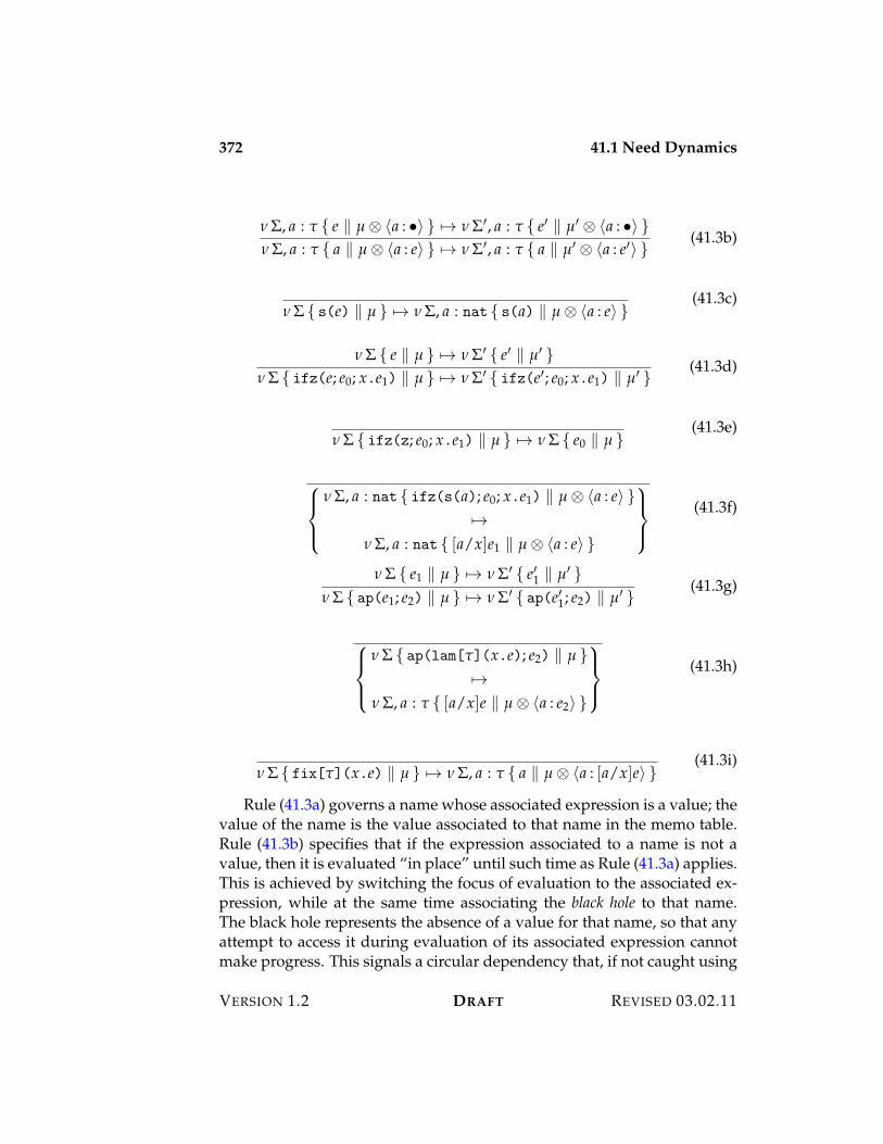
372 41.1 Need Dynamics
0 $, a : " { e / µ E ?a : •@ } 53 0 $%, a : " { e% / µ% E ?a : •@ }0 $, a : " { a / µ E ?a : e@ } 53 0 $%, a : " { a / µ% E ?a : e%@ }
(41.3b)
0 $ { s(e) / µ } 53 0 $, a : nat { s(a) / µ E ?a : e@ }(41.3c)
0 $ { e / µ } 53 0 $% { e% / µ% }0 $ { ifz(e; e0; x.e1) / µ } 53 0 $% { ifz(e%; e0; x.e1) / µ% }
(41.3d)
0 $ { ifz(z; e0; x.e1) / µ } 53 0 $ { e0 / µ }(41.3e)
,-.
-/
0 $, a : nat { ifz(s(a); e0; x.e1) / µ E ?a : e@ }53
0 $, a : nat { [a/x]e1 / µ E ?a : e@ }
0-1
-2
(41.3f)
0 $ { e1 / µ } 53 0 $% { e%1 / µ% }0 $ { ap(e1; e2) / µ } 53 0 $% { ap(e%1; e2) / µ% }
(41.3g)
,-.
-/
0 $ { ap(lam["](x.e); e2) / µ }53
0 $, a : " { [a/x]e / µ E ?a : e2@ }
0-1
-2
(41.3h)
0 $ { fix["](x.e) / µ } 53 0 $, a : " { a / µ E ?a : [a/x]e@ }(41.3i)
Rule (41.3a) governs a name whose associated expression is a value; thevalue of the name is the value associated to that name in the memo table.Rule (41.3b) specifies that if the expression associated to a name is not avalue, then it is evaluated “in place” until such time as Rule (41.3a) applies.This is achieved by switching the focus of evaluation to the associated ex-pression, while at the same time associating the black hole to that name.The black hole represents the absence of a value for that name, so that anyattempt to access it during evaluation of its associated expression cannotmake progress. This signals a circular dependency that, if not caught using
VERSION 1.2 DRAFT REVISED 03.02.11
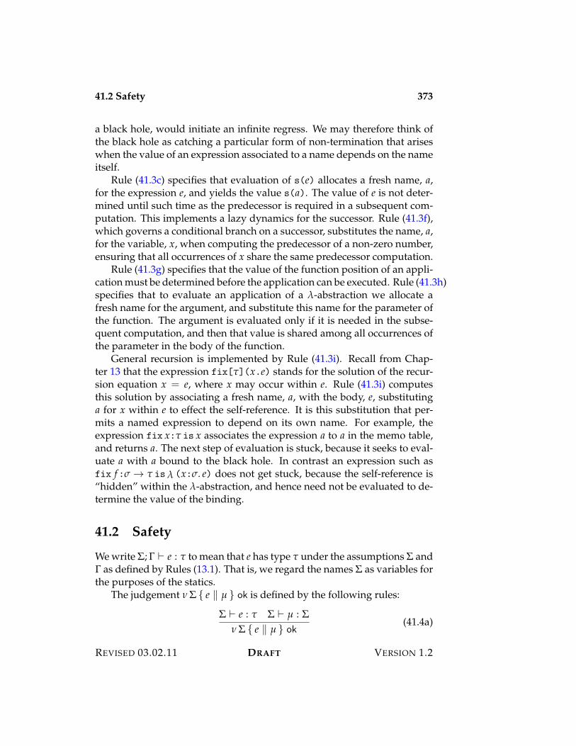
41.2 Safety 373
a black hole, would initiate an infinite regress. We may therefore think ofthe black hole as catching a particular form of non-termination that ariseswhen the value of an expression associated to a name depends on the nameitself.
Rule (41.3c) specifies that evaluation of s(e) allocates a fresh name, a,for the expression e, and yields the value s(a). The value of e is not deter-mined until such time as the predecessor is required in a subsequent com-putation. This implements a lazy dynamics for the successor. Rule (41.3f),which governs a conditional branch on a successor, substitutes the name, a,for the variable, x, when computing the predecessor of a non-zero number,ensuring that all occurrences of x share the same predecessor computation.
Rule (41.3g) specifies that the value of the function position of an appli-cation must be determined before the application can be executed. Rule (41.3h)specifies that to evaluate an application of a !-abstraction we allocate afresh name for the argument, and substitute this name for the parameter ofthe function. The argument is evaluated only if it is needed in the subse-quent computation, and then that value is shared among all occurrences ofthe parameter in the body of the function.
General recursion is implemented by Rule (41.3i). Recall from Chap-ter 13 that the expression fix["](x.e) stands for the solution of the recur-sion equation x = e, where x may occur within e. Rule (41.3i) computesthis solution by associating a fresh name, a, with the body, e, substitutinga for x within e to effect the self-reference. It is this substitution that per-mits a named expression to depend on its own name. For example, theexpression fix x:" is x associates the expression a to a in the memo table,and returns a. The next step of evaluation is stuck, because it seeks to eval-uate a with a bound to the black hole. In contrast an expression such asfix f:& 3 " is! (x:&. e) does not get stuck, because the self-reference is“hidden” within the !-abstraction, and hence need not be evaluated to de-termine the value of the binding.
41.2 Safety
We write $; ! ) e : " to mean that e has type " under the assumptions $ and! as defined by Rules (13.1). That is, we regard the names $ as variables forthe purposes of the statics.
The judgement 0 $ { e / µ } ok is defined by the following rules:
$ ) e : " $ ) µ : $0 $ { e / µ } ok
(41.4a)
REVISED 03.02.11 DRAFT VERSION 1.2
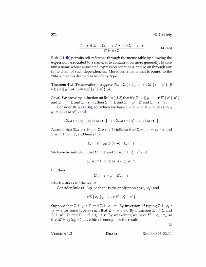
374 41.2 Safety
&a : " + $ µ(a) = e ,= • =; $% ) e : "
$% ) µ : $(41.4b)
Rule (41.4b) permits self-reference through the memo table by allowing theexpression associated to a name, a, to contain a, or, more generally, to con-tain a name whose associated expression contains a, and so on through anyfinite chain of such dependencies. Moreover, a name that is bound to the“black hole” is deemed to be of any type.
Theorem 41.1 (Preservation). Suppose that 0 $ { e / µ } 53 0 $% { e% / µ% }. If0 $ { e / µ } ok, then 0 $% { e% / µ% } ok.
Proof. We prove by induction on Rules (41.3) that if 0 $ { e / µ } 53 0 $% { e% / µ% }and $ ) µ : $ and $ ) e : ", then $% L $ and $% ) µ% : $% and $% ) e% : ".
Consider Rule (41.3b), for which we have e = e% = a, µ = µ0 E ?a : e0@,µ% = µ%
0 E ?a : e%0@, and
0 $, a : " { e0 / µ0 E ?a : •@ } 53 0 $%, a : " { e%0 / µ%0 E ?a : •@ }.
Assume that $, a : " ) µ : $, a : ". It follows that $, a : " ) e0 : " and$, a : " ) µ0 : $, and hence that
$, a : " ) µ0 E ?a : •@ : $, a : ".
We have by induction that $% L $ and $%, a : " ) e%0 : "% and
$%, a : " ) µ0 E ?a : •@ : $, a : ".
But then$%, a : " ) µ% : $%, a : ",
which suffices for the result.Consider Rule (41.3g), so that e is the application ap(e1; e2) and
0 $ { e1 / µ } 53 0 $% { e%1 / µ% }.
Suppose that $ ) µ : $ and $ ) e : ". By inversion of typing $ ) e1 :"2 3 " for some type "2 such that $ ) e2 : "2. By induction $% L $ and$% ) µ% : $% and $% ) e%1 : "2 3 ". By weakening we have $% ) e2 : "2, sothat $% ) ap(e%1; e2) : ", which is enough for the result.
VERSION 1.2 DRAFT REVISED 03.02.11
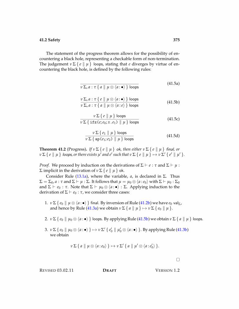
41.2 Safety 375
The statement of the progress theorem allows for the possibility of en-countering a black hole, representing a checkable form of non-termination.The judgement 0 $ { e / µ } loops, stating that e diverges by virtue of en-countering the black hole, is defined by the following rules:
0 $, a : " { a / µ E ?a : •@ } loops(41.5a)
0 $, a : " { e / µ E ?a : •@ } loops
0 $, a : " { a / µ E ?a : e@ } loops(41.5b)
0 $ { e / µ } loops
0 $ { ifz(e; e0; x.e1) / µ } loops(41.5c)
0 $ { e1 / µ } loops
0 $ { ap(e1; e2) / µ } loops(41.5d)
Theorem 41.2 (Progress). If 0 $ { e / µ } ok, then either 0 $ { e / µ } final, or0 $ { e / µ } loops, or there exists µ% and e% such that 0 $ { e / µ } 53 0 $% { e% / µ% }.
Proof. We proceed by induction on the derivations of $ ) e : " and $ ) µ :$ implicit in the derivation of 0 $ { e / µ } ok.
Consider Rule (13.1a), where the variable, a, is declared in $. Thus$ = $0, a : " and $ ) µ : $. It follows that µ = µ0 E ?a : e0@ with $ ) µ0 : $0and $ ) e0 : ". Note that $ ) µ0 E ?a : •@ : $. Applying induction to thederivation of $ ) e0 : ", we consider three cases:
1. 0 $ { e0 / µ E ?a : •@ } final. By inversion of Rule (41.2b) we have e0 val$,and hence by Rule (41.3a) we obtain 0 $ { a / µ } 53 0 $ { e0 / µ }.
2. 0 $ { e0 / µ0 E ?a : •@ } loops. By applying Rule (41.5b) we obtain 0 $ { a / µ } loops.
3. 0 $ { e0 / µ0 E ?a : •@ } 53 0 $% { e%0 / µ%0 E ?a : •@ }. By applying Rule (41.3b)
we obtain
0 $ { a / µ E ?a : e0@ } 53 0 $% { a / µ% E ?a : e%0@ }.
REVISED 03.02.11 DRAFT VERSION 1.2
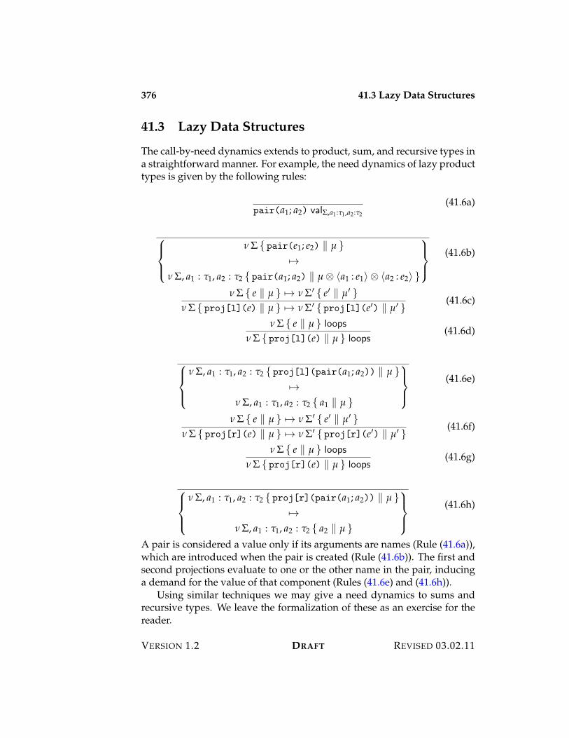
376 41.3 Lazy Data Structures
41.3 Lazy Data Structures
The call-by-need dynamics extends to product, sum, and recursive types ina straightforward manner. For example, the need dynamics of lazy producttypes is given by the following rules:
pair(a1; a2) val$,a1:"1,a2:"2
(41.6a)
,-.
-/
0 $ { pair(e1; e2) / µ }53
0 $, a1 : "1, a2 : "2 { pair(a1; a2) / µ E ?a1 : e1@ E ?a2 : e2@ }
0-1
-2
(41.6b)
0 $ { e / µ } 53 0 $% { e% / µ% }0 $ { proj[l](e) / µ } 53 0 $% { proj[l](e%) / µ% }
(41.6c)
0 $ { e / µ } loops
0 $ { proj[l](e) / µ } loops(41.6d)
,-.
-/
0 $, a1 : "1, a2 : "2 { proj[l](pair(a1; a2)) / µ }53
0 $, a1 : "1, a2 : "2 { a1 / µ }
0-1
-2
(41.6e)
0 $ { e / µ } 53 0 $% { e% / µ% }0 $ { proj[r](e) / µ } 53 0 $% { proj[r](e%) / µ% }
(41.6f)
0 $ { e / µ } loops
0 $ { proj[r](e) / µ } loops(41.6g)
,-.
-/
0 $, a1 : "1, a2 : "2 { proj[r](pair(a1; a2)) / µ }53
0 $, a1 : "1, a2 : "2 { a2 / µ }
0-1
-2
(41.6h)
A pair is considered a value only if its arguments are names (Rule (41.6a)),which are introduced when the pair is created (Rule (41.6b)). The first andsecond projections evaluate to one or the other name in the pair, inducinga demand for the value of that component (Rules (41.6e) and (41.6h)).
Using similar techniques we may give a need dynamics to sums andrecursive types. We leave the formalization of these as an exercise for thereader.
VERSION 1.2 DRAFT REVISED 03.02.11
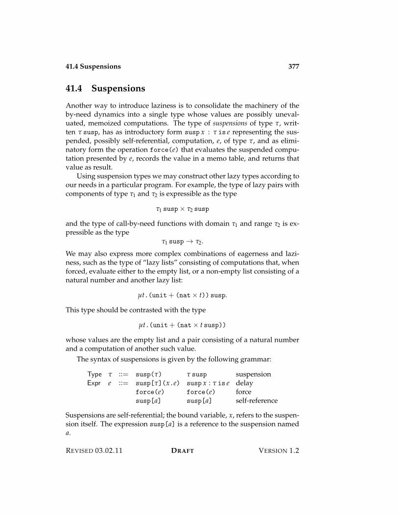
41.4 Suspensions 377
41.4 Suspensions
Another way to introduce laziness is to consolidate the machinery of theby-need dynamics into a single type whose values are possibly uneval-uated, memoized computations. The type of suspensions of type ", writ-ten " susp, has as introductory form susp x : " is e representing the sus-pended, possibly self-referential, computation, e, of type ", and as elimi-natory form the operation force(e) that evaluates the suspended compu-tation presented by e, records the value in a memo table, and returns thatvalue as result.
Using suspension types we may construct other lazy types according toour needs in a particular program. For example, the type of lazy pairs withcomponents of type "1 and "2 is expressible as the type
"1 susp< "2 susp
and the type of call-by-need functions with domain "1 and range "2 is ex-pressible as the type
"1 susp 3 "2.
We may also express more complex combinations of eagerness and lazi-ness, such as the type of “lazy lists” consisting of computations that, whenforced, evaluate either to the empty list, or a non-empty list consisting of anatural number and another lazy list:
µt.(unit+ (nat< t)) susp.
This type should be contrasted with the type
µt.(unit+ (nat< t susp))
whose values are the empty list and a pair consisting of a natural numberand a computation of another such value.
The syntax of suspensions is given by the following grammar:
Type " ::= susp(") " susp suspensionExpr e ::= susp["](x.e) susp x : " is e delay
force(e) force(e) forcesusp[a] susp[a] self-reference
Suspensions are self-referential; the bound variable, x, refers to the suspen-sion itself. The expression susp[a] is a reference to the suspension nameda.
REVISED 03.02.11 DRAFT VERSION 1.2
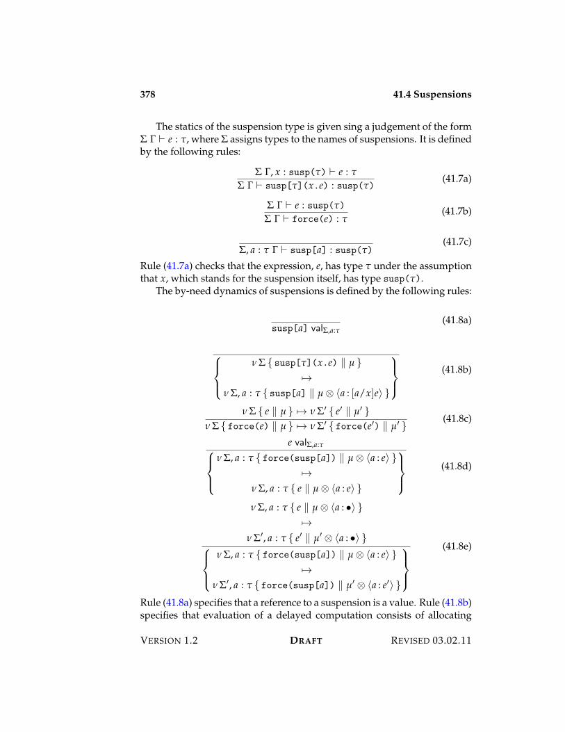
378 41.4 Suspensions
The statics of the suspension type is given sing a judgement of the form$ ! ) e : ", where $ assigns types to the names of suspensions. It is definedby the following rules:
$ !, x : susp(") ) e : "
$ ! ) susp["](x.e) : susp(")(41.7a)
$ ! ) e : susp(")
$ ! ) force(e) : "(41.7b)
$, a : " ! ) susp[a] : susp(")(41.7c)
Rule (41.7a) checks that the expression, e, has type " under the assumptionthat x, which stands for the suspension itself, has type susp(").
The by-need dynamics of suspensions is defined by the following rules:
susp[a] val$,a:"(41.8a)
,-.
-/
0 $ { susp["](x.e) / µ }53
0 $, a : " { susp[a] / µ E ?a : [a/x]e@ }
0-1
-2
(41.8b)
0 $ { e / µ } 53 0 $% { e% / µ% }0 $ { force(e) / µ } 53 0 $% { force(e%) / µ% }
(41.8c)
e val$,a:",-.
-/
0 $, a : " { force(susp[a]) / µ E ?a : e@ }53
0 $, a : " { e / µ E ?a : e@ }
0-1
-2(41.8d)
0 $, a : " { e / µ E ?a : •@ }53
0 $%, a : " { e% / µ% E ?a : •@ },-.
-/
0 $, a : " { force(susp[a]) / µ E ?a : e@ }53
0 $%, a : " { force(susp[a]) / µ% E ?a : e%@ }
0-1
-2
(41.8e)
Rule (41.8a) specifies that a reference to a suspension is a value. Rule (41.8b)specifies that evaluation of a delayed computation consists of allocating
VERSION 1.2 DRAFT REVISED 03.02.11
41.5 Exercises 379
a fresh name for it in the memo table, and returning a reference to thatsuspension. Rules (41.8c) to (41.8e) specify that demanding the value of asuspension forces evaluation of the suspended computation, which is thenstored in the memo table and returned as result.
41.5 Exercises
REVISED 03.02.11 DRAFT VERSION 1.2

380 41.5 Exercises
VERSION 1.2 DRAFT REVISED 03.02.11
Chapter 42
Polarization
Up to this point we have frequently encountered arbitrary choices in thedynamics of various language constructs. For example, when specifyingthe dynamics of pairs, we must choose, rather arbitrarily, between the lazydynamics, in which all pairs are values regardless of the value status oftheir components, and the eager dynamics, in which a pair is a value onlyif its components are both values. We could even consider a half-eager (or,if you are a pessimist, half-lazy) dynamics, in which a pair is a value onlyif, say, the first component is a value, but without regard to the second.Although the latter choice seems rather arbitrary, it is no less so than thechoice between a fully lazy or a fully eager dynamics.
Similar questions arise with sums (all injections are values, or only in-jections of values are values), recursive types (all folds are values, or onlyfolds whose arguments are values), and function types (functions shouldbe called by-name or by-value). Whole languages are built around adher-ence to one policy or another. For example, Haskell decrees that products,sums, and recursive types are to be lazy, and functions are to be called byname, whereas ML decrees the exact opposite policy. Not only are thesechoices arbitrary, but it is also unclear why they should be linked. For ex-ample, one could very sensibly decree that products, sums, and recursivetypes are lazy, yet impose a call-by-value discipline on functions. Or onecould have eager products, sums, and recursive types, yet insist on call-by-name. It is not at all clear which of these points in the space of choices isright; each language has its adherents, each has its drawbacks, and eachhas its advantages.
Are we therefore stuck in a tarpit of subjectivity? No! The way out isto recognize that these distinctions should not be imposed by the language
382 42.1 Polarization
designer, but rather are choices that are to be made by the programmer.This is achieved by recognizing that differences in dynamics reflect funda-mental type distinctions that are being obscured by languages that imposeone policy or another. We can have both eager and lazy pairs in the samelanguage by simply distinguishing them as two distinct types, and sim-ilarly we can have both eager and lazy sums in the same language, andboth by-name and by-value function spaces, by providing sufficient typedistinctions as to make the choice available to the programmer.
In this chapter we will introduce polarization to distinguish types basedon whether their elements are defined by their values (the positive types) orby their behavior (the negative types). Put in other terms, positive types are“eager” (determined by their values), whereas negative types are “lazy”(determined by their behavior). Since positive types are defined by theirvalues, they are eliminated by pattern matching against these values. Sim-ilarly, since negative types are defined by their behavior under a range ofexperiments, they are eliminated by performing an experiment on them.
To make these symmetries explicit we formalize polarization using atechnique called focusing, or focalization.1 A focused presentation of a pro-gramming language distinguishes three general forms of expression, (pos-itive and negative) values, (positive and negative) continuations, and (neutral)computations. Besides exposing the symmetries in a polarized type sys-tem, focusing also clarifies the design of the control machine introducedin Chapter 31. In a focused framework stacks are just continuations, andstates are just computations; there is no need for any ad hoc apparatus toexplain the flow of control in a program.
42.1 Polarization
Polarization consists of distinguishing positive from negative types accord-ing to the following two principles:
1. A positive type is defined by its introduction rules, which specify thevalues of that type in terms of other values. The elimination rules areinversions that specify a computation by pattern matching on valuesof that type.
2. A negative type is defined by its elimination rules, which specify theobservations that may be performed on elements of that type. The
1More precisely, we employ a weak form of focusing, rather than the stricter forms con-sidered elsewhere in the literature.
VERSION 1.2 DRAFT REVISED 03.02.11
42.2 Focusing 383
introduction rules specify the values of that type by specifying howthey respond to observations.
Based on this characterization we can anticipate that the type of naturalnumbers would be positive, since it is defined by zero and successor, whereasfunction types would be negative, since they are characterized by their be-havior when applied, and not by their internal structure.
The language L±{nat"} is a polarized formulation of L{nat"} inwhich the syntax of types is given by the following grammar:
PType "+ ::= dn("$) 6 "$ suspensionnat nat naturals
NType "$ ::= up("+) M "+ inclusionparr("+
1 ; "$2 ) "+
1 " "$2 partial function
The types 6 "$ and M "+ effect a polarity shift from negative to positive andpositive to negative, respectively. Intuitively, the shifted type M "+ is justthe inclusion of positive into negative values, whereas the shifted type 6 "$
represents the type of suspended computations of negative type.The domain of the negative function type is required to be positive, but
its range is negative. This allows us to form right-iterated function types
"+1 " ("+
2 " (. . . ("+n$1 " "$
n )))
directly, but to form a left-iterated function type requires shifting,
6 ("+1 " "$
2 )" "$,
to turn the negative function type into a positive type. Conversely, shiftingis needed to define a function whose range is positive, "+
1 " M "+2 .
42.2 Focusing
The syntax of L±{nat"} is motivated by the polarization of its types. Foreach polarity we have a sort of values and a sort of continuations with
REVISED 03.02.11 DRAFT VERSION 1.2
384 42.3 Statics
which we may create (neutral) computations.
PVal v+ ::= z z zeros(v+) s(v+) successordel-(e) del-(e) delay
PCont k+ ::= ifz(e0; x.e1) ifz(e0; x.e1) conditionalforce-(k$) force-(k$) evaluate
NVal v$ ::= lam["+](x.e) ! (x:"+. e) abstractiondel+(v+) del+(v+) inclusionfix(x.v$) fix x is v$ recursion
NCont k$ ::= ap(v+; k$) ap(v+; k$) applicationforce+(x.e) force+(x.e) evaluate
Comp e ::= ret(v$) ret(v$) returncut+(v+; k+) v+ $ k+ cutcut-(v$; k$) v$ $ k$ cut
The positive values include the numerals, and the negative values includefunctions. In addition we may delay a computation of a negative value toform a positive value using del-(e), and we may consider a positive valueto be a negative value using del+(v+). The positive continuations includethe conditional branch, sans argument, and the negative continuations in-clude application sites for functions consisting of a positive argument valueand a continuation for the negative result. In addition we include positivecontinuations to force the computation of a suspended negative value, andto extract an included positive value. Computations, which correspond tomachine states, consist of returned negative values (these are final states),states passing a positive value to a positive continuation, and states pass-ing a negative value to a negative continuation. General recursion appearsas a form of negative value; the recursion is unrolled when it is made thesubject of an observation.
42.3 Statics
The statics of L±{nat"} consists of a collection of rules for deriving judge-ments of the following forms:
• Positive values: ! ) v+ : "+.
• Positive continuations: ! ) k+ : "+ > /$.
• Negative values: ! ) v$ : "$.
VERSION 1.2 DRAFT REVISED 03.02.11
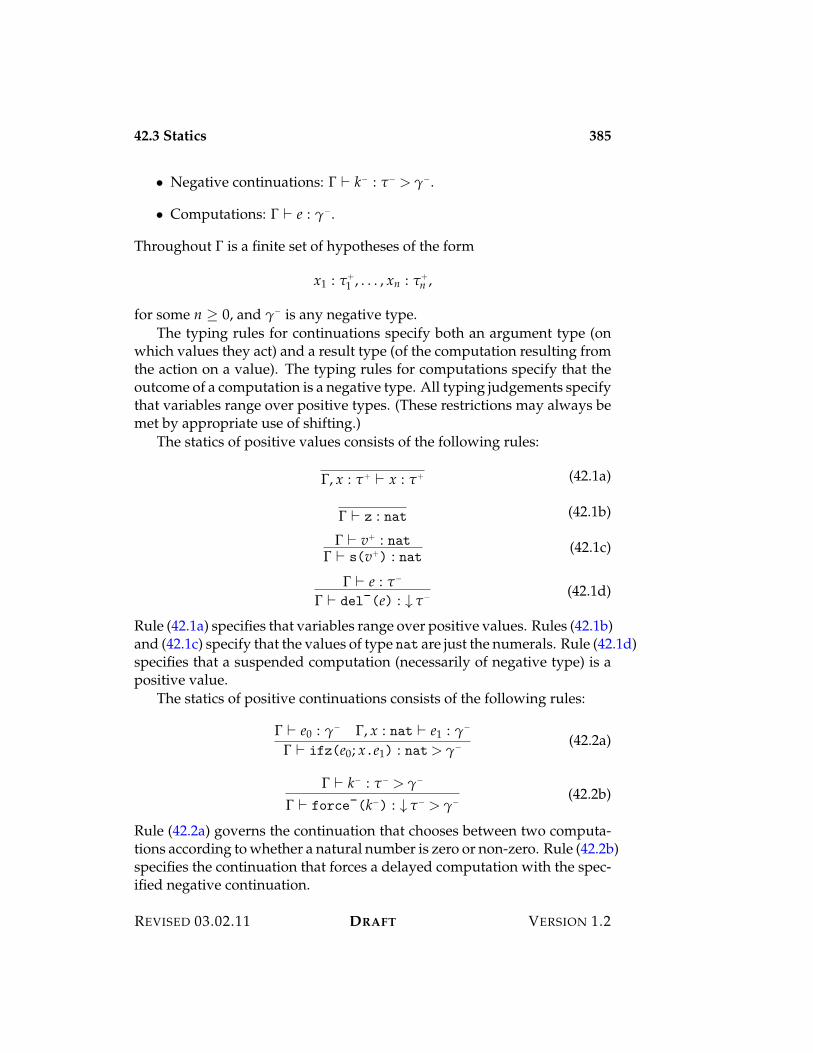
42.3 Statics 385
• Negative continuations: ! ) k$ : "$ > /$.
• Computations: ! ) e : /$.
Throughout ! is a finite set of hypotheses of the form
x1 : "+1 , . . . , xn : "+
n ,
for some n 7 0, and /$ is any negative type.The typing rules for continuations specify both an argument type (on
which values they act) and a result type (of the computation resulting fromthe action on a value). The typing rules for computations specify that theoutcome of a computation is a negative type. All typing judgements specifythat variables range over positive types. (These restrictions may always bemet by appropriate use of shifting.)
The statics of positive values consists of the following rules:
!, x : "+ ) x : "+ (42.1a)
! ) z : nat (42.1b)
! ) v+ : nat! ) s(v+) : nat (42.1c)
! ) e : "$
! ) del-(e) : 6 "$ (42.1d)
Rule (42.1a) specifies that variables range over positive values. Rules (42.1b)and (42.1c) specify that the values of type nat are just the numerals. Rule (42.1d)specifies that a suspended computation (necessarily of negative type) is apositive value.
The statics of positive continuations consists of the following rules:
! ) e0 : /$ !, x : nat ) e1 : /$
! ) ifz(e0; x.e1) : nat> /$ (42.2a)
! ) k$ : "$ > /$
! ) force-(k$) : 6 "$ > /$(42.2b)
Rule (42.2a) governs the continuation that chooses between two computa-tions according to whether a natural number is zero or non-zero. Rule (42.2b)specifies the continuation that forces a delayed computation with the spec-ified negative continuation.
REVISED 03.02.11 DRAFT VERSION 1.2
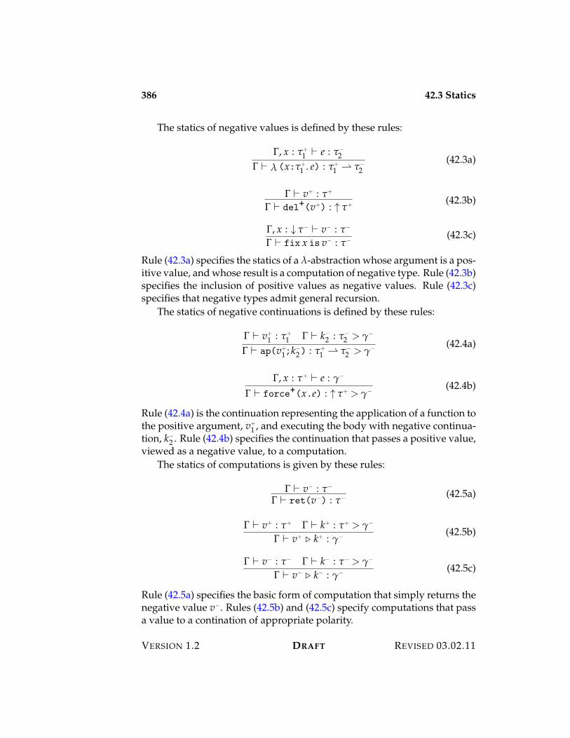
386 42.3 Statics
The statics of negative values is defined by these rules:
!, x : "+1 ) e : "$
2! ) ! (x:"+
1 . e) : "+1 " "$
2(42.3a)
! ) v+ : "+
! ) del+(v+) : M "+ (42.3b)
!, x : 6 "$ ) v$ : "$
! ) fix x is v$ : "$(42.3c)
Rule (42.3a) specifies the statics of a !-abstraction whose argument is a pos-itive value, and whose result is a computation of negative type. Rule (42.3b)specifies the inclusion of positive values as negative values. Rule (42.3c)specifies that negative types admit general recursion.
The statics of negative continuations is defined by these rules:
! ) v+1 : "+
1 ! ) k$2 : "$
2 > /$
! ) ap(v+1 ; k$
2) : "+1 " "$
2 > /$ (42.4a)
!, x : "+ ) e : /$
! ) force+(x.e) : M "+ > /$(42.4b)
Rule (42.4a) is the continuation representing the application of a function tothe positive argument, v+
1 , and executing the body with negative continua-tion, k$
2 . Rule (42.4b) specifies the continuation that passes a positive value,viewed as a negative value, to a computation.
The statics of computations is given by these rules:
! ) v$ : "$
! ) ret(v$) : "$ (42.5a)
! ) v+ : "+ ! ) k+ : "+ > /$
! ) v+ $ k+ : /$ (42.5b)
! ) v$ : "$ ! ) k$ : "$ > /$
! ) v$ $ k$ : /$ (42.5c)
Rule (42.5a) specifies the basic form of computation that simply returns thenegative value v$. Rules (42.5b) and (42.5c) specify computations that passa value to a contination of appropriate polarity.
VERSION 1.2 DRAFT REVISED 03.02.11
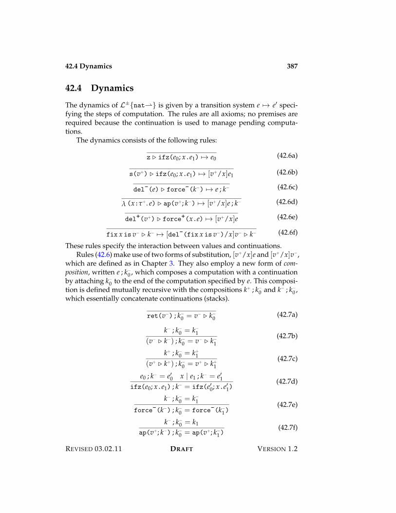
42.4 Dynamics 387
42.4 Dynamics
The dynamics of L±{nat"} is given by a transition system e 53 e% speci-fying the steps of computation. The rules are all axioms; no premises arerequired because the continuation is used to manage pending computa-tions.
The dynamics consists of the following rules:
z $ ifz(e0; x.e1) 53 e0 (42.6a)
s(v+) $ ifz(e0; x.e1) 53 [v+/x]e1 (42.6b)
del-(e) $ force-(k$) 53 e ; k$ (42.6c)
! (x:"+. e) $ ap(v+; k$) 53 [v+/x]e ; k$ (42.6d)
del+(v+) $ force+(x.e) 53 [v+/x]e (42.6e)
fix x is v$ $ k$ 53 [del-(fix x is v$)/x]v$ $ k$ (42.6f)
These rules specify the interaction between values and continuations.Rules (42.6) make use of two forms of substitution, [v+/x]e and [v+/x]v$,
which are defined as in Chapter 3. They also employ a new form of com-position, written e ; k$
0 , which composes a computation with a continuationby attaching k$
0 to the end of the computation specified by e. This composi-tion is defined mutually recursive with the compositions k+ ; k$
0 and k$ ; k$0 ,
which essentially concatenate continuations (stacks).
ret(v$) ; k$0 = v$ $ k$
0 (42.7a)
k$ ; k$0 = k$
1
(v$ $ k$) ; k$0 = v$ $ k$
1(42.7b)
k+ ; k$0 = k+
1
(v+ $ k+) ; k$0 = v+ $ k+
1(42.7c)
e0 ; k$ = e%0 x | e1 ; k$ = e%1ifz(e0; x.e1) ; k$ = ifz(e%0; x.e%1)
(42.7d)
k$ ; k$0 = k$
1
force-(k$) ; k$0 = force-(k$
1)(42.7e)
k$ ; k$0 = k1
ap(v+; k$) ; k$0 = ap(v+; k$
1)(42.7f)
REVISED 03.02.11 DRAFT VERSION 1.2
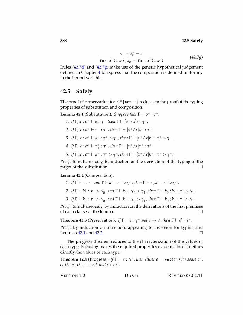
388 42.5 Safety
x | e ; k$0 = e%
force+(x.e) ; k$0 = force+(x.e%)
(42.7g)
Rules (42.7d) and (42.7g) make use of the generic hypothetical judgementdefined in Chapter 4 to express that the composition is defined uniformlyin the bound variable.
42.5 Safety
The proof of preservation for L±{nat"} reduces to the proof of the typingproperties of substitution and composition.
Lemma 42.1 (Substitution). Suppose that ! ) v+ : &+.
1. If !, x : &+ ) e : /$, then ! ) [v+/x]e : /$.
2. If !, x : &+ ) v$ : "$, then ! ) [v+/x]v$ : "$.
3. If !, x : &+ ) k+ : "+ > /$, then ! ) [v+/x]k+ : "+ > /$.
4. If !, x : &+ ) v+1 : "+, then ! ) [v+/x]v+
1 : "+.
5. If !, x : &+ ) k$ : "$ > /$, then ! ) [v+/x]k$ : "$ > /$.
Proof. Simultaneously, by induction on the derivation of the typing of thetarget of the substitution.
Lemma 42.2 (Composition).
1. If ! ) e : "$ and ! ) k$ : "$ > /$, then ! ) e ; k$ : "$ > /$.
2. If ! ) k+0 : "+ > /$
0 , and ! ) k$1 : /$
0 > /$1 , then ! ) k+
0 ; k$1 : "+ > /$
1 .
3. If ! ) k$0 : "$ > /$
0 , and ! ) k$1 : /$
0 > /$1 , then ! ) k$
0 ; k$1 : "$ > /$
1 .
Proof. Simultaneously, by induction on the derivations of the first premisesof each clause of the lemma.
Theorem 42.3 (Preservation). If ! ) e : /$ and e 53 e%, then ! ) e% : /$.
Proof. By induction on transition, appealing to inversion for typing andLemmas 42.1 and 42.2.
The progress theorem reduces to the characterization of the values ofeach type. Focusing makes the required properties evident, since it definesdirectly the values of each type.
Theorem 42.4 (Progress). If ! ) e : /$, then either e = ret(v$) for some v$,or there exists e% such that e 53 e%.
VERSION 1.2 DRAFT REVISED 03.02.11
42.6 Definability 389
42.6 Definability
The syntax of L±{nat"} exposes the symmetries between positive andnegative types, and hence between eager and lazy computation. It is not,however, especially convenient for writing programs because it requiresthat each computation in a program be expressed in the stilted form of avalue juxtaposed with a continuation. It would be useful to have a morenatural syntax that is translatable into the present language.
But the question of what is a natural syntax begs the very question thatmotivated the language in the first place!
Editorial Notes
This chapter under construction.
42.7 Exercises
REVISED 03.02.11 DRAFT VERSION 1.2

390 42.7 Exercises
VERSION 1.2 DRAFT REVISED 03.02.11

Part XVI
Parallelism

Chapter 43
Nested Parallelism
Parallel computation seeks to reduce the running times of programs by al-lowing many computations to be carried out simultaneously. For example,if one wishes to add two numbers, each given by a complex computation,we may consider evaluating the addends simultaneously, then computingtheir sum. The ability to exploit parallelism is limited by the dependenciesamong parts of a program. Obviously, if one computation depends on theresult of another, then we have no choice but to execute them sequentiallyso that we may propagate the result of the first to the second. Consequently,the fewer dependencies among sub-computations, the greater the opportu-nities for parallelism. This argues for functional models of computation,because the possibility of mutation of shared assignables imposes sequen-tialization constraints on imperative code.
In this chapter we discuss nested parallelism in which we nest parallelcomputations within one another in a hierarchical manner. Nested paral-lelism is sometimes called fork-join parallelism to emphasize the hierarchi-cal structure arising from forking two (or more) parallel computations, thenjoining these computations to combine their results before proceeding. Wewill consider two forms of dynamics for nested parallelism. The first is astructural dynamics in which a single transition on a compound expres-sion may involve multiple transitions on its constituent expressions. Thesecond is a cost dynamics (introduced in Chapter 10) that focuses atten-tion on the sequential and parallel complexity (also known as the work anddepth) of a parallel program by associating a series-parallel graph with eachcomputation.
394 43.1 Binary Fork-Join
43.1 Binary Fork-Join
We begin with a parallel language whose sole source of parallelism is thesimultaneous evaluation of two variable bindings. This is modelled by aconstruct of the form letpar x1 = e1 and x2 = e2 in e, in which we bind twovariables, x1 and x2, to two expressions, e1 and e2, respectively, for usewithin a single expression, e. This represents a simple fork-join primitive inwhich e1 and e2 may be evaluated independently of one another, with theirresults combined by the expression e. Some other forms of parallelism maybe defined in terms of this primitive. For example, a parallel pair constructmight be defined as the expression
letpar x1 = e1 and x2 = e2 in ?x1, x2@,
which evaluates the components of the pair in parallel, then constructs thepair itself from these values.
The abstract syntax of the parallel binding construct is given by the ab-stract binding tree
letpar(e1; e2; x1.x2.e),
which makes clear that the variables x1 and x2 are bound only within e, andnot within their bindings. This ensures that evaluation of e1 is independentof evaluation of e2, and vice versa. The typing rule for an expression of thisform is given as follows:
! ) e1 : "1 ! ) e2 : "2 !, x1 : "1, x2 : "2 ) e : "! ) letpar(e1; e2; x1.x2.e) : "
(43.1)
Although we emphasize the case of binary parallelism, it should be clearthat this construct easily generalizes to n-way parallelism for any staticvalue of n. One may also define an n-way parallel let construct from thebinary parallel let by cascading binary splits. (For a treatment of n-wayparallelism for a dynamic value of n, see Section 43.3 on page 400.)
We will give both a sequential and a parallel dynamics of the parallellet construct. The definition of the sequential dynamics as a transitionjudgement of the form e 53seq e% is entirely straightforward:
e1 53 e%1letpar(e1; e2; x1.x2.e) 53seq letpar(e%1; e2; x1.x2.e)
(43.2a)
e1 val e2 53 e%2letpar(e1; e2; x1.x2.e) 53seq letpar(e1; e%2; x1.x2.e)
(43.2b)
VERSION 1.2 DRAFT REVISED 03.02.11
43.1 Binary Fork-Join 395
e1 val e2 val
letpar(e1; e2; x1.x2.e) 53seq [e1, e2/x1, x2]e(43.2c)
The parallel dynamics is given by a transition judgement of the form e 53par
e%, defined as follows:
e1 53par e%1 e2 53par e%2letpar(e1; e2; x1.x2.e) 53par letpar(e%1; e%2; x1.x2.e)
(43.3a)
e1 53par e%1 e2 val
letpar(e1; e2; x1.x2.e) 53par letpar(e%1; e2; x1.x2.e)(43.3b)
e1 val e2 53par e%2letpar(e1; e2; x1.x2.e) 53par letpar(e1; e%2; x1.x2.e)
(43.3c)
e1 val e2 val
letpar(e1; e2; x1.x2.e) 53par [e1, e2/x1, x2]e(43.3d)
The parallel dynamics is idealized in that it abstracts away from any limi-tations on parallelism that would necessarily be imposed in practice by theavailability of computing resources.
An important advantage of the present approach is captured by the im-plicit parallelism theorem, which states that the sequential and the paralleldynamics coincide. This means that one need never be concerned with thesemantics of a parallel program (its meaning is determined by the sequen-tial dynamics), but only with its performance. Since the sequential dynamicsis deterministic (every expression has at most one value), the implicit par-allelism theorem implies that the parallel dynamics is also deterministic.This clearly distinguishes parallelism, which is deterministic, from concur-rency, which is non-deterministic (see Chapters 45 and 46 for more on con-currency).
A proof of the implicit parallelism theorem may be given by giving anevaluation dynamics, e " v, in the style of Chapter 10, and showing that
e 531par v iff e " v iff e 531
seq v
(where v is a closed expression such that v val). The crucial rule of theevaluation dynamics is the one governing the parallel let construct:
e1 " v1 e2 " v2 [v1, v2/x1, x2]e " vletpar(e1; e2; x1.x2.e) " v
(43.4)
It is easy to show that the sequential dynamics agrees with the evalua-tion dynamics by a straightforward extension of the proof of Theorem 10.2on page 85.
REVISED 03.02.11 DRAFT VERSION 1.2
396 43.1 Binary Fork-Join
Lemma 43.1. e 531seq v iff e " v.
Proof. It suffices to show that if e 53seq e% and e% " v, then e " v, and that ife1 531
seq v1 and e2 531seq v2 and [v1, v2/x1, x2]e 531
seq v, then
letpar x1 = e1 and x2 = e2 in e 531seq v.
We leave the details of the proof as an exercise for the reader.
By a similar argument we may show that the parallel dynamics alsoagrees with the evaluation dynamics, and hence with the sequential dy-namics.
Lemma 43.2. e 531par v iff e " v.
Proof. It suffices to show that if e 53par e% and e% " v, then e " v, and that ife1 531
par v1 and e2 531par v2 and [v1, v2/x1, x2]e 531
par v, then
letpar x1 = e1 and x2 = e2 in e 531par v.
The proof of the first is by a straightforward induction on the parallel dy-namics. The proof of the second proceeds by simultaneous induction onthe derivations of e1 531
par v1 and e2 531par v2. If e1 = v1 with v1 val and
e2 = v2 with v2 val, then the result follows immediately from the thirdpremise. If e2 = v2 but e1 53par e%1 531
par v1, then by induction we havethat letpar x1 = e%1 and x2 = v2 in e 531
par v, and hence the result follows byan application of Rule (43.3b). The symmetric case follows similarly by anapplication of Rule (43.3c), and in case both e1 and e2 take a step, the resultfollows by induction and Rule (43.3a).
Theorem 43.3 (Implicit Parallelism). The sequential and parallel dynamics co-incide: for all v val, e 531
seq v iff e 531par v.
Proof. By Lemmas 43.1 and 43.2.
Theorem 43.3 states that parallelism is implicit in that the use of a paral-lel evaluation strategy does not affect the semantics of a program, but onlyits efficiency. The program means the same thing under a parallel executionstrategy as it does under a sequential one. Correctness concerns are fac-tored out, focusing attention on time (and space) complexity of a parallelexecution strategy.
VERSION 1.2 DRAFT REVISED 03.02.11
43.2 Cost Dynamics 397
43.2 Cost Dynamics
In this section we define a parallel cost dynamics that assigns a cost graph tothe evaluation of an expression. Cost graphs are defined by the followinggrammar:
Cost c ::= 0 zero cost1 unit costc1 E c2 parallel combinationc1 N c2 sequential combination
A cost graph is a form of series-parallel directed acyclic graph, with a des-ignated source node and sink node. For 0 the graph consists of one nodeand no edges, with the source and sink both being the node itself. For 1 thegraph consists of two nodes and one edge directed from the source to thesink. For c1 E c2, if g1 and g2 are the graphs of c1 and c2, respectively, thenthe graph has two additional nodes, a source node with two edges to thesource nodes of g1 and g2, and a sink node, with edges from the sink nodesof g1 and g2 to it. Finally, for c1 N c2, where g1 and g2 are the graphs of c1and c2, the graph has as source node the source of g1, as sink node the sinkof g2, and an edge from the sink of g1 to the source of g2.
The intuition behind a cost graph is that nodes represent subcompu-tations of an overall computation, and edges represent sequentiality con-straints stating that one computation depends on the result of another, andhence cannot be started before the one on which it depends completes. Theproduct of two graphs represents parallelism opportunities in which there areno sequentiality constraints between the two computations. The assign-ment of source and sink nodes reflects the overhead of forking two parallelcomputations and joining them after they have both completed.
We associate with each cost graph two numeric measures, the work,wk(c), and the depth, dp(c). The work is defined by the following equa-tions:
wk(c) =
,----.
----/
0 if c = 01 if c = 1wk(c1) + wk(c2) if c = c1 E c2
wk(c1) + wk(c2) if c = c1 N c2
(43.5)
REVISED 03.02.11 DRAFT VERSION 1.2
398 43.2 Cost Dynamics
The depth is defined by the following equations:
dp(c) =
,----.
----/
0 if c = 01 if c = 1max(dp(c1), dp(c2)) if c = c1 E c2
dp(c1) + dp(c2) if c = c1 N c2
(43.6)
Informally, the work of a cost graph determines the total number of com-putation steps represented by the cost graph, and thus corresponds to thesequential complexity of the computation. The depth of the cost graph de-termines the critical path length, the length of the longest dependency chainwithin the computation, which imposes a lower bound on the parallel com-plexity of a computation. The critical path length is the least number ofsequential steps that can be taken, even if we have unlimited parallelismavailable to us, because of steps that can be taken only after the completionof another.
In Chapter 10 we introduced cost dynamics as a means of assigning timecomplexity to evaluation. The proof of Theorem 10.7 on page 88 shows thate "k v iff e 53k v. That is, the step complexity of an evaluation of e to a valuev is just the number of transitions required to derive e 531 v. Here we usecost graphs as the measure of complexity, then relate these cost graphs tothe structural dynamics given in Section 43.1 on page 394.
The judgement e "c v, where e is a closed expression, v is a closed value,and c is a cost graph specifies the cost dynamics. By definition we arrangethat e "0 e when e val. The cost assignment for let is given by the followingrule:
e1 "c1 v1 e2 "c2 v2 [v1, v2/x1, x2]e "c vletpar(e1; e2; x1.x2.e) "(c1Ec2)N1Nc v
(43.7)
The cost assignment specifies that, under ideal conditions, e1 and e2 are tobe evaluated in parallel, and that their results are to be propagated to e.The cost of fork and join is implicit in the parallel combination of costs, andassign unit cost to the substitution because we expect it to be implementedin practice by a constant-time mechanism for updating an environment.The cost dynamics of other language constructs is specified in a similarmanner, using only sequential combination so as to isolate the source ofparallelism to the let construct.
Two simple facts about the cost dynamics are important to keep inmind. First, the cost assignment does not influence the outcome.
Lemma 43.4. e " v iff e "c v for some c.
VERSION 1.2 DRAFT REVISED 03.02.11
43.2 Cost Dynamics 399
Proof. From right to left, erase the cost assignments to obtain an evalua-tion derivation. From left to right, decorate the evaluation derivations withcosts as determined by the rules defining the cost dynamics.
Second, the cost of evaluating an expression is uniquely determined.
Lemma 43.5. If e "c v and e "c% v, then c is c%.
Proof. A routine induction on the derivation of e "c v.
The link between the cost dynamics and the structural dynamics givenin the preceding section is established by the following theorem, whichstates that the work cost is the sequential complexity, and the depth cost isthe parallel complexity, of the computation.
Theorem 43.6. If e "c v, then e 53wseq v and e 53d
par v, where w = wk(c)and d = dp(c). Conversely, if e 53w
seq v, then there exists c such that e "c vwith wk(c) = w, and if e 53d
par v%, then there exists c% such that e "c% v% withdp(c%) = d. Therefore if e 53w
seq v and e 53dpar v%, then v is v% and e "c v for some
c such that wk(c) = w and dp(c) = d.
Proof. The first part is proved by induction on the derivation of e "c v,the interesting case being Rule (43.7). By induction we have e1 53w1
seq v1,e2 53w2
seq v2, and [v1, v2/x1, x2]e 53wseq v, where w1 = wk(c1), w2 = wk(c2),
and w = wk(c). By pasting together derivations we obtain a derivation
letpar(e1; e2; x1.x2.e) 53w1seq letpar(v1; e2; x1.x2.e)
53w2seq letpar(v1; v2; x1.x2.e)
53seq [v1, v2/x1, x2]e53w
seq v.
Noting that wk((c1 E c2)N 1 N c) = w1 + w2 + 1 + w completes the proof.Similarly, we have by induction that e1 53d1
par v1, e2 53d2par v2, and e 53d
par v,where d1 = dp(c1), d2 = dp(c2), and d = dp(c). Assume, without loss ofgenerality, that d1 ( d2 (otherwise simply swap the roles of d1 and d2 inwhat follows). We may paste together derivations as follows:
letpar(e1; e2; x1.x2.e) 53d1par letpar(v1; e%2; x1.x2.e)
53d2$d1par letpar(v1; v2; x1.x2.e)
53par [v1, v2/x1, x2]e
53dpar v.
REVISED 03.02.11 DRAFT VERSION 1.2
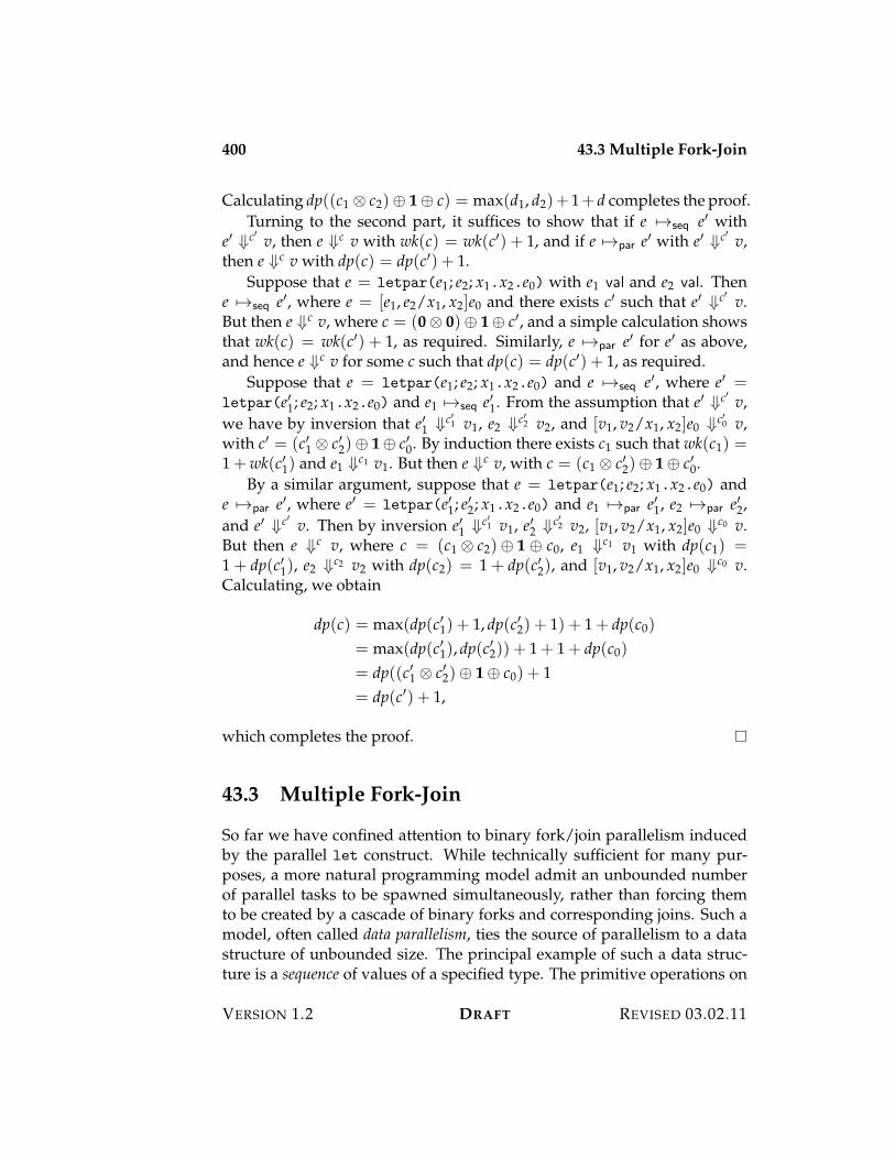
400 43.3 Multiple Fork-Join
Calculating dp((c1 E c2)N 1 N c) = max(d1, d2)+ 1+ d completes the proof.Turning to the second part, it suffices to show that if e 53seq e% with
e% "c% v, then e "c v with wk(c) = wk(c%) + 1, and if e 53par e% with e% "c% v,then e "c v with dp(c) = dp(c%) + 1.
Suppose that e = letpar(e1; e2; x1.x2.e0) with e1 val and e2 val. Thene 53seq e%, where e = [e1, e2/x1, x2]e0 and there exists c% such that e% "c% v.But then e "c v, where c = (0 E 0)N 1 N c%, and a simple calculation showsthat wk(c) = wk(c%) + 1, as required. Similarly, e 53par e% for e% as above,and hence e "c v for some c such that dp(c) = dp(c%) + 1, as required.
Suppose that e = letpar(e1; e2; x1.x2.e0) and e 53seq e%, where e% =letpar(e%1; e2; x1.x2.e0) and e1 53seq e%1. From the assumption that e% "c% v,we have by inversion that e%1 "c%1 v1, e2 "c%2 v2, and [v1, v2/x1, x2]e0 "c%0 v,with c% = (c%1 E c%2)N 1 N c%0. By induction there exists c1 such that wk(c1) =1 + wk(c%1) and e1 "c1 v1. But then e "c v, with c = (c1 E c%2)N 1 N c%0.
By a similar argument, suppose that e = letpar(e1; e2; x1.x2.e0) ande 53par e%, where e% = letpar(e%1; e%2; x1.x2.e0) and e1 53par e%1, e2 53par e%2,and e% "c% v. Then by inversion e%1 "c%1 v1, e%2 "c%2 v2, [v1, v2/x1, x2]e0 "c0 v.But then e "c v, where c = (c1 E c2)N 1 N c0, e1 "c1 v1 with dp(c1) =1 + dp(c%1), e2 "c2 v2 with dp(c2) = 1 + dp(c%2), and [v1, v2/x1, x2]e0 "c0 v.Calculating, we obtain
dp(c) = max(dp(c%1) + 1, dp(c%2) + 1) + 1 + dp(c0)
= max(dp(c%1), dp(c%2)) + 1 + 1 + dp(c0)
= dp((c%1 E c%2)N 1 N c0) + 1= dp(c%) + 1,
which completes the proof.
43.3 Multiple Fork-Join
So far we have confined attention to binary fork/join parallelism inducedby the parallel let construct. While technically sufficient for many pur-poses, a more natural programming model admit an unbounded numberof parallel tasks to be spawned simultaneously, rather than forcing themto be created by a cascade of binary forks and corresponding joins. Such amodel, often called data parallelism, ties the source of parallelism to a datastructure of unbounded size. The principal example of such a data struc-ture is a sequence of values of a specified type. The primitive operations on
VERSION 1.2 DRAFT REVISED 03.02.11
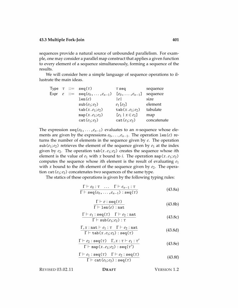
43.3 Multiple Fork-Join 401
sequences provide a natural source of unbounded parallelism. For exam-ple, one may consider a parallel map construct that applies a given functionto every element of a sequence simultaneously, forming a sequence of theresults.
We will consider here a simple language of sequence operations to il-lustrate the main ideas.
Type " ::= seq(") " seq sequenceExpr e ::= seq(e0, . . . ,en$1) [e0, . . . ,en$1] sequence
len(e) |e| sizesub(e1; e2) e1[e2] elementtab(x.e1; e2) tab(x.e1; e2) tabulatemap(x.e1; e2) [e1 | x + e2] mapcat(e1; e2) cat(e1; e2) concatenate
The expression seq(e0, . . . ,en$1) evaluates to an n-sequence whose ele-ments are given by the expressions e0, . . . , en$1. The operation len(e) re-turns the number of elements in the sequence given by e. The operationsub(e1; e2) retrieves the element of the sequence given by e1 at the indexgiven by e2. The operation tab(x.e1; e2) creates the sequence whose ithelement is the value of e1 with x bound to i. The operation map(x.e1; e2)
computes the sequence whose ith element is the result of evaluating e1with x bound to the ith element of the sequence given by e2. The opera-tion cat(e1; e2) concatenates two sequences of the same type.
The statics of these operations is given by the following typing rules:
! ) e0 : " . . . ! ) en$1 : "
! ) seq(e0, . . . ,en$1) : seq(")(43.8a)
! ) e : seq(")
! ) len(e) : nat(43.8b)
! ) e1 : seq(") ! ) e2 : nat! ) sub(e1; e2) : "
(43.8c)
!, x : nat ) e1 : " ! ) e2 : nat! ) tab(x.e1; e2) : seq(")
(43.8d)
! ) e2 : seq(") !, x : " ) e1 : "%
! ) map(x.e1; e2) : seq("%)(43.8e)
! ) e1 : seq(") ! ) e2 : seq(")
! ) cat(e1; e2) : seq(")(43.8f)
REVISED 03.02.11 DRAFT VERSION 1.2
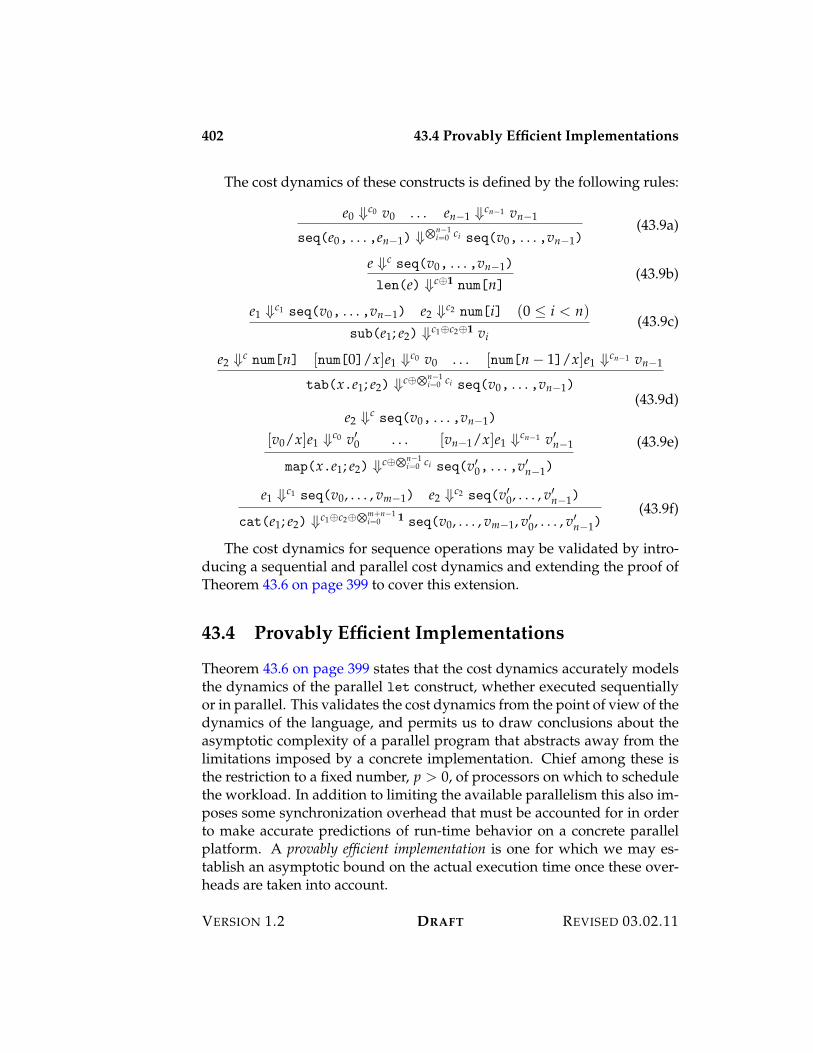
402 43.4 Provably Efficient Implementations
The cost dynamics of these constructs is defined by the following rules:
e0 "c0 v0 . . . en$1 "cn$1 vn$1
seq(e0, . . . ,en$1) "3n$1
i=0 ci seq(v0, . . . ,vn$1)(43.9a)
e "c seq(v0, . . . ,vn$1)
len(e) "cN1 num[n](43.9b)
e1 "c1 seq(v0, . . . ,vn$1) e2 "c2 num[i] (0 ( i < n)sub(e1; e2) "c1Nc2N1 vi
(43.9c)
e2 "c num[n] [num[0]/x]e1 "c0 v0 . . . [num[n $ 1]/x]e1 "cn$1 vn$1
tab(x.e1; e2) "cN3n$1i=0 ci seq(v0, . . . ,vn$1)
(43.9d)e2 "c seq(v0, . . . ,vn$1)
[v0/x]e1 "c0 v%0 . . . [vn$1/x]e1 "cn$1 v%n$1
map(x.e1; e2) "cN3n$1i=0 ci seq(v%0, . . . ,v%n$1)
(43.9e)
e1 "c1 seq(v0, . . . , vm$1) e2 "c2 seq(v%0, . . . , v%n$1)
cat(e1; e2) "c1Nc2N3m+n$1
i=0 1 seq(v0, . . . , vm$1, v%0, . . . , v%n$1)(43.9f)
The cost dynamics for sequence operations may be validated by intro-ducing a sequential and parallel cost dynamics and extending the proof ofTheorem 43.6 on page 399 to cover this extension.
43.4 Provably Efficient Implementations
Theorem 43.6 on page 399 states that the cost dynamics accurately modelsthe dynamics of the parallel let construct, whether executed sequentiallyor in parallel. This validates the cost dynamics from the point of view of thedynamics of the language, and permits us to draw conclusions about theasymptotic complexity of a parallel program that abstracts away from thelimitations imposed by a concrete implementation. Chief among these isthe restriction to a fixed number, p > 0, of processors on which to schedulethe workload. In addition to limiting the available parallelism this also im-poses some synchronization overhead that must be accounted for in orderto make accurate predictions of run-time behavior on a concrete parallelplatform. A provably efficient implementation is one for which we may es-tablish an asymptotic bound on the actual execution time once these over-heads are taken into account.
VERSION 1.2 DRAFT REVISED 03.02.11
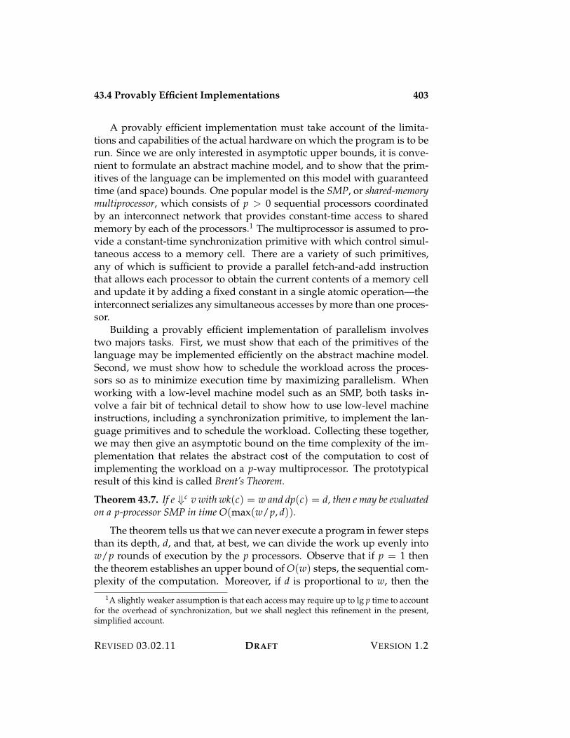
43.4 Provably Efficient Implementations 403
A provably efficient implementation must take account of the limita-tions and capabilities of the actual hardware on which the program is to berun. Since we are only interested in asymptotic upper bounds, it is conve-nient to formulate an abstract machine model, and to show that the prim-itives of the language can be implemented on this model with guaranteedtime (and space) bounds. One popular model is the SMP, or shared-memorymultiprocessor, which consists of p > 0 sequential processors coordinatedby an interconnect network that provides constant-time access to sharedmemory by each of the processors.1 The multiprocessor is assumed to pro-vide a constant-time synchronization primitive with which control simul-taneous access to a memory cell. There are a variety of such primitives,any of which is sufficient to provide a parallel fetch-and-add instructionthat allows each processor to obtain the current contents of a memory celland update it by adding a fixed constant in a single atomic operation—theinterconnect serializes any simultaneous accesses by more than one proces-sor.
Building a provably efficient implementation of parallelism involvestwo majors tasks. First, we must show that each of the primitives of thelanguage may be implemented efficiently on the abstract machine model.Second, we must show how to schedule the workload across the proces-sors so as to minimize execution time by maximizing parallelism. Whenworking with a low-level machine model such as an SMP, both tasks in-volve a fair bit of technical detail to show how to use low-level machineinstructions, including a synchronization primitive, to implement the lan-guage primitives and to schedule the workload. Collecting these together,we may then give an asymptotic bound on the time complexity of the im-plementation that relates the abstract cost of the computation to cost ofimplementing the workload on a p-way multiprocessor. The prototypicalresult of this kind is called Brent’s Theorem.
Theorem 43.7. If e "c v with wk(c) = w and dp(c) = d, then e may be evaluatedon a p-processor SMP in time O(max(w/p, d)).
The theorem tells us that we can never execute a program in fewer stepsthan its depth, d, and that, at best, we can divide the work up evenly intow/p rounds of execution by the p processors. Observe that if p = 1 thenthe theorem establishes an upper bound of O(w) steps, the sequential com-plexity of the computation. Moreover, if d is proportional to w, then the
1A slightly weaker assumption is that each access may require up to lg p time to accountfor the overhead of synchronization, but we shall neglect this refinement in the present,simplified account.
REVISED 03.02.11 DRAFT VERSION 1.2
404 43.4 Provably Efficient Implementations
overall time is again O(w), which is to say that we are unable to exploitparallelism in that case.
This motivates the definition of a useful figure of merit, called the par-allelizability ratio, which is the ratio, w/d, of work to depth. If w/d O p,then the program is said to be parallelizable, because then w/p O d, andwe may therefore reduce running time by using p processors at each step.If, on the other hand, the parallelizability ratio is a constant, then d willdominate w/p, and we will have little opportunity to exploit parallelism toreduce running time. It is not known, in general, whether a problem admitsa parallelizable solution. The best we can say, on present knowledge, is thatthere are algorithms for some problems that have a high degree of paral-lelizability, and there are problems for which no such algorithm is known.It is a open problem in complexity theory to characterize which problemsare parallelizable, and which are not.
To illustrate the essential ingredients of the proof of Brent’s Theorem wewill consider a dynamics that models the scheduling of work onto p par-allel processors, each of which implements the dynamics of L{nat"} asdescribed in Chapter 13. The dynamics consists of two transition relationsdefined on states of the form
0 x1 : "1, . . . xn : "n { ?x1 : e1@ E . . . E ?xn : en@ }.
Such a state represents the remaining work of a computation, decomposedinto n tasks, with each task binding its value to a variable. Importantly, wedo not distinguish states that differ in the order of the variable declarationsor variable bindings.
The occurrences of variables in a state determine the dependency order-ing among the tasks: if xi occurs free in xj, then ej cannot be evaluatedbefore evaluation of ei is complete. Such dependencies reflect data flow de-pendencies among the tasks, and are therefore manifestations of the depthcomplexity of the program. A closed expression ei in a state is said to beready in that state; otherwise, ei is said to be blocked, awaiting completion ofevaluation of the expression on which it depends.
We will consider two forms of state transition, the local and the global.Local transitions represent the steps of computation of the individual pro-cessors, which we will model using the dynamics of L{nat"} given inChapter 13 as a guide. Global transitions represent the scheduling andload-balancing steps that allocate tasks to processors with the intent ofmaximizing parallelism insofar as possible consistently with the depen-dency ordering among the tasks.
VERSION 1.2 DRAFT REVISED 03.02.11
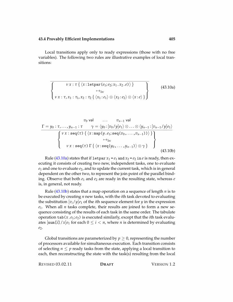
43.4 Provably Efficient Implementations 405
Local transitions apply only to ready expressions (those with no freevariables). The following two rules are illustrative examples of local tran-sitions:
,-.
-/
0 x : " { ?x : letpar(e1; e2; x1.x2.e)@ }53loc
0 x : ", x1 : "1, x2 : "2 { ?x1 : e1@ E ?x2 : e2@ E ?x : e@ }
0-1
-2
(43.10a)
v0 val . . . vn$1 val
! = y0 : ", . . . , yn$1 : " / = ?y0 : [v0/y]e1@ E . . . E ?yn$1 : [vn$1/y]e1@,-.
-/
0 x : seq(") { ?x : map(y.e1; seq(v0, . . . ,vn$1))@ }53loc
0 x : seq(") ! { ?x : seq(y0, . . . ,yn$1)@ E / }
0-1
-2
(43.10b)
Rule (43.10a) states that if letpar x1 = e1 and x2 = e2 in e is ready, then ex-ecuting it consists of creating two new, independent tasks, one to evaluatee1 and one to evaluate e2, and to update the current task, which is in generaldependent on the other two, to represent the join point of the parallel bind-ing. Observe that both e1 and e2 are ready in the resulting state, whereas eis, in general, not ready.
Rule (43.10b) states that a map operation on a sequence of length n is tobe executed by creating n new tasks, with the ith task devoted to evaluatingthe substitution [vi/y]e1 of the ith sequence element for y in the expressione1. When all n tasks complete, their results are joined to form a new se-quence consisting of the results of each task in the same order. The tabulateoperation tab(x.e1; e2) is executed similarly, except that the ith task evalu-ates [num[i]/x]e1 for each 0 ( i < n, where n is determined by evaluatinge2.
Global transitions are parameterized by p 7 0, representing the numberof processors available for simultaneous execution. Each transition consistsof selecting n ( p ready tasks from the state, applying a local transition toeach, then reconstructing the state with the task(s) resulting from the local
REVISED 03.02.11 DRAFT VERSION 1.2
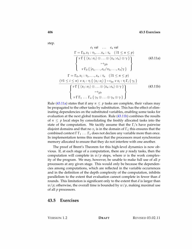
406 43.5 Exercises
step.e1 val . . . en val
! = !0, x1 : "1, . . . xn : "n ('1 ( n ( p),-.
-/
0 ! { ?x1 : e1@ E . . . E ?xn : en@ E / }53glo
0 !0 { [e1, . . . , en/x1, . . . , xn]/ }
0-1
-2
(43.11a)
! = !0, x1 : "1, . . . , xn : "n ('1 ( n ( p)(&1 ( i ( n) 0 xi : "i { ?xi : ei@ } 53loc 0 xi : "i !i { /i }
,-.
-/
0 ! { ?x1 : e1@ E . . . E ?xn : en@ E / }53glo
0 ! !1 . . . !n { /1 E . . . E /n E / }
0-1
-2
(43.11b)
Rule (43.11a) states that if any n ( p tasks are complete, their values maybe propagated to the other tasks by substitution. This has the effect of elim-inating dependencies on the substituted variables, enabling some tasks forevaluation at the next global transition. Rule (43.11b) combines the resultsof n ( p local steps by consolidating the freshly allocated tasks into thestate of the computation. We tacitly assume that the !i’s have pairwisedisjoint domains and that no xj is in the domain of !i; this ensures that thecombined context ! !1 . . . !n does not declare any variable more than once.In implementation terms this means that the processors must synchronizememory allocated to ensure that they do not interfere with one another.
The proof of Brent’s Theorem for this high-level dynamics is now ob-vious. If, at each stage of a computation, there are p ready tasks, then thecomputation will complete in w/p steps, where w is the work complex-ity of the program. We may, however, be unable to make full use of all pprocessors at any given stage. This would only be because the dependen-cies among computations, which are reflected in the variable occurrencesand in the definition of the depth complexity of the computation, inhibitsparallelism to the extent that evaluation cannot complete in fewer than drounds. This limitation is significant only to the extent that d is larger thanw/p; otherwise, the overall time is bounded by w/p, making maximal useof all p processors.
43.5 Exercises
VERSION 1.2 DRAFT REVISED 03.02.11
Chapter 44
Futures and Speculation
A future is a computation whose evaluation is initiated in advance of anydemand for its value. Like a suspension, a future represents a value that isto be determined later. Unlike a suspension, a future is always evaluated,regardless of whether its value is actually required. In a sequential settingfutures are of little interest; a future of type " is just an expression of type ".In a parallel setting, however, futures are of interest because they provide ameans of initiating a parallel computation whose result is not needed until(presumably) much later, by which time it will have been completed.
The prototypical example of the use of futures is to implementing pipelin-ing, a method for overlapping the stages of a multistage computation tothe fullest extent possible. This minimizes the latency caused by one stagewaiting for the completion of a previous stage by allowing the two stagesto proceed in parallel until such time as an explicit dependency is encoun-tered. Ideally, the computation of the result of an earlier stage is completedby the time a later stage requires it. At worst the later stage must be delayeduntil the earlier stage completes, incurring what is known as a pipeline stall.
A suspension is a delayed computation whose result may or may not beneeded for the overall computation to finish. Speculation is a parallel dy-namics for suspensions in which suspended computations are executed inparallel with the main thread of computation without regard to whether thesuspension is forced. If the value of the suspension is eventually required,then speculation pays off, but if not, the effort to evaluate it wasted. Specu-lation is therefore not work-efficient: if the value of the suspension is neverneeded, more work has been undertaken than is necessary to determine theoutcome of the computation. Speculation can be useful in situations wherethere is an excess of computing resources available, more than can be used
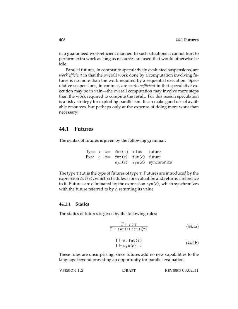
408 44.1 Futures
in a guaranteed work-efficient manner. In such situations it cannot hurt toperform extra work as long as resources are used that would otherwise beidle.
Parallel futures, in contrast to speculatively evaluated suspensions, arework efficient in that the overall work done by a computation involving fu-tures is no more than the work required by a sequential execution. Spec-ulative suspensions, in contrast, are work inefficient in that speculative ex-ecution may be in vain—the overall computation may involve more stepsthan the work required to compute the result. For this reason speculationis a risky strategy for exploiting parallelism. It can make good use of avail-able resources, but perhaps only at the expense of doing more work thannecessary!
44.1 Futures
The syntax of futures is given by the following grammar:
Type " ::= fut(") " fut futureExpr e ::= fut(e) fut(e) future
syn(e) syn(e) synchronize
The type " fut is the type of futures of type ". Futures are introduced by theexpression fut(e), which schedules e for evaluation and returns a referenceto it. Futures are eliminated by the expression syn(e), which synchronizeswith the future referred to by e, returning its value.
44.1.1 Statics
The statics of futures is given by the following rules:
! ) e : "! ) fut(e) : fut(")
(44.1a)
! ) e : fut(")! ) syn(e) : "
(44.1b)
These rules are unsurprising, since futures add no new capabilities to thelanguage beyond providing an opportunity for parallel evaluation.
VERSION 1.2 DRAFT REVISED 03.02.11
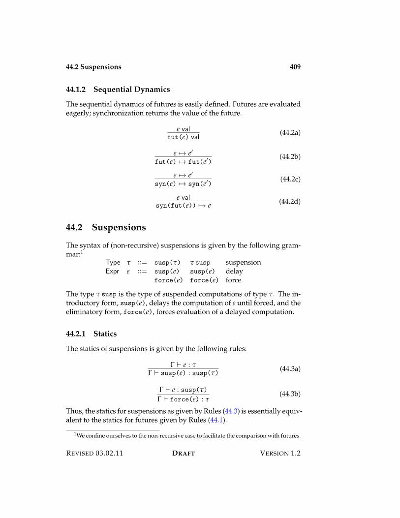
44.2 Suspensions 409
44.1.2 Sequential Dynamics
The sequential dynamics of futures is easily defined. Futures are evaluatedeagerly; synchronization returns the value of the future.
e valfut(e) val
(44.2a)
e 53 e%fut(e) 53 fut(e%)
(44.2b)
e 53 e%syn(e) 53 syn(e%) (44.2c)
e valsyn(fut(e)) 53 e (44.2d)
44.2 Suspensions
The syntax of (non-recursive) suspensions is given by the following gram-mar:1
Type " ::= susp(") " susp suspensionExpr e ::= susp(e) susp(e) delay
force(e) force(e) force
The type " susp is the type of suspended computations of type ". The in-troductory form, susp(e), delays the computation of e until forced, and theeliminatory form, force(e), forces evaluation of a delayed computation.
44.2.1 Statics
The statics of suspensions is given by the following rules:
! ) e : "! ) susp(e) : susp(")
(44.3a)
! ) e : susp(")
! ) force(e) : "(44.3b)
Thus, the statics for suspensions as given by Rules (44.3) is essentially equiv-alent to the statics for futures given by Rules (44.1).
1We confine ourselves to the non-recursive case to facilitate the comparison with futures.
REVISED 03.02.11 DRAFT VERSION 1.2
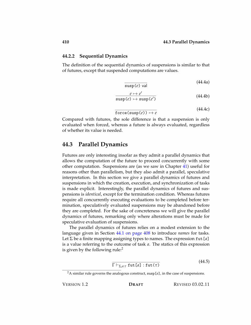
410 44.3 Parallel Dynamics
44.2.2 Sequential Dynamics
The definition of the sequential dynamics of suspensions is similar to thatof futures, except that suspended computations are values.
susp(e) val(44.4a)
e 53 e%susp(e) 53 susp(e%) (44.4b)
force(susp(e)) 53 e(44.4c)
Compared with futures, the sole difference is that a suspension is onlyevaluated when forced, whereas a future is always evaluated, regardlessof whether its value is needed.
44.3 Parallel Dynamics
Futures are only interesting insofar as they admit a parallel dynamics thatallows the computation of the future to proceed concurrently with someother computation. Suspensions are (as we saw in Chapter 41) useful forreasons other than parallelism, but they also admit a parallel, speculativeinterpretation. In this section we give a parallel dynamics of futures andsuspensions in which the creation, execution, and synchronization of tasksis made explicit. Interestingly, the parallel dynamics of futures and sus-pensions is identical, except for the termination condition. Whereas futuresrequire all concurrently executing evaluations to be completed before ter-mination, speculatively evaluated suspensions may be abandoned beforethey are completed. For the sake of concreteness we will give the paralleldynamics of futures, remarking only where alterations must be made forspeculative evaluation of suspensions.
The parallel dynamics of futures relies on a modest extension to thelanguage given in Section 44.1 on page 408 to introduce names for tasks.Let $ be a finite mapping assigning types to names. The expression fut[a]is a value referring to the outcome of task a. The statics of this expressionis given by the following rule:2
! )$,a:" fut[a] : fut(")(44.5)
2A similar rule governs the analogous construct, susp[a], in the case of suspensions.
VERSION 1.2 DRAFT REVISED 03.02.11
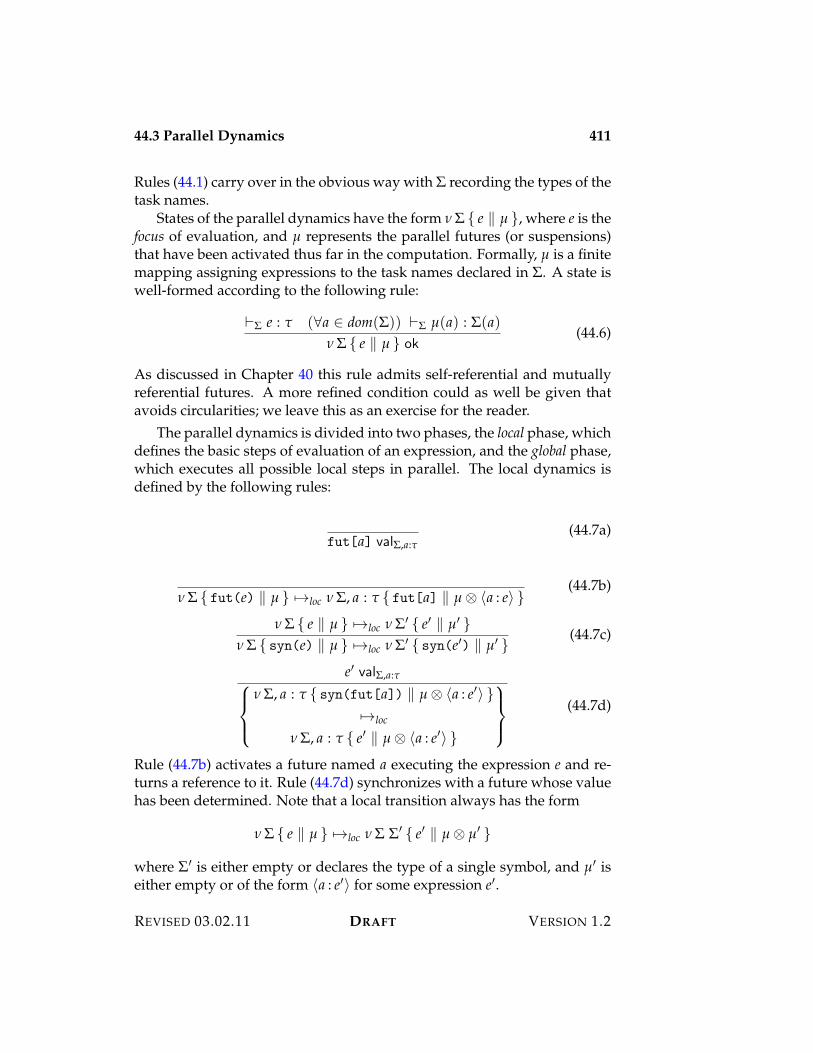
44.3 Parallel Dynamics 411
Rules (44.1) carry over in the obvious way with $ recording the types of thetask names.
States of the parallel dynamics have the form 0 $ { e / µ }, where e is thefocus of evaluation, and µ represents the parallel futures (or suspensions)that have been activated thus far in the computation. Formally, µ is a finitemapping assigning expressions to the task names declared in $. A state iswell-formed according to the following rule:
)$ e : " (&a + dom($)) )$ µ(a) : $(a)0 $ { e / µ } ok
(44.6)
As discussed in Chapter 40 this rule admits self-referential and mutuallyreferential futures. A more refined condition could as well be given thatavoids circularities; we leave this as an exercise for the reader.
The parallel dynamics is divided into two phases, the local phase, whichdefines the basic steps of evaluation of an expression, and the global phase,which executes all possible local steps in parallel. The local dynamics isdefined by the following rules:
fut[a] val$,a:"(44.7a)
0 $ { fut(e) / µ } 53loc 0 $, a : " { fut[a] / µ E ?a : e@ }(44.7b)
0 $ { e / µ } 53loc 0 $% { e% / µ% }0 $ { syn(e) / µ } 53loc 0 $% { syn(e%) / µ% }
(44.7c)
e% val$,a:",-.
-/
0 $, a : " { syn(fut[a]) / µ E ?a : e%@ }53loc
0 $, a : " { e% / µ E ?a : e%@ }
0-1
-2(44.7d)
Rule (44.7b) activates a future named a executing the expression e and re-turns a reference to it. Rule (44.7d) synchronizes with a future whose valuehas been determined. Note that a local transition always has the form
0 $ { e / µ } 53loc 0 $ $% { e% / µ E µ% }
where $% is either empty or declares the type of a single symbol, and µ% iseither empty or of the form ?a : e%@ for some expression e%.
REVISED 03.02.11 DRAFT VERSION 1.2
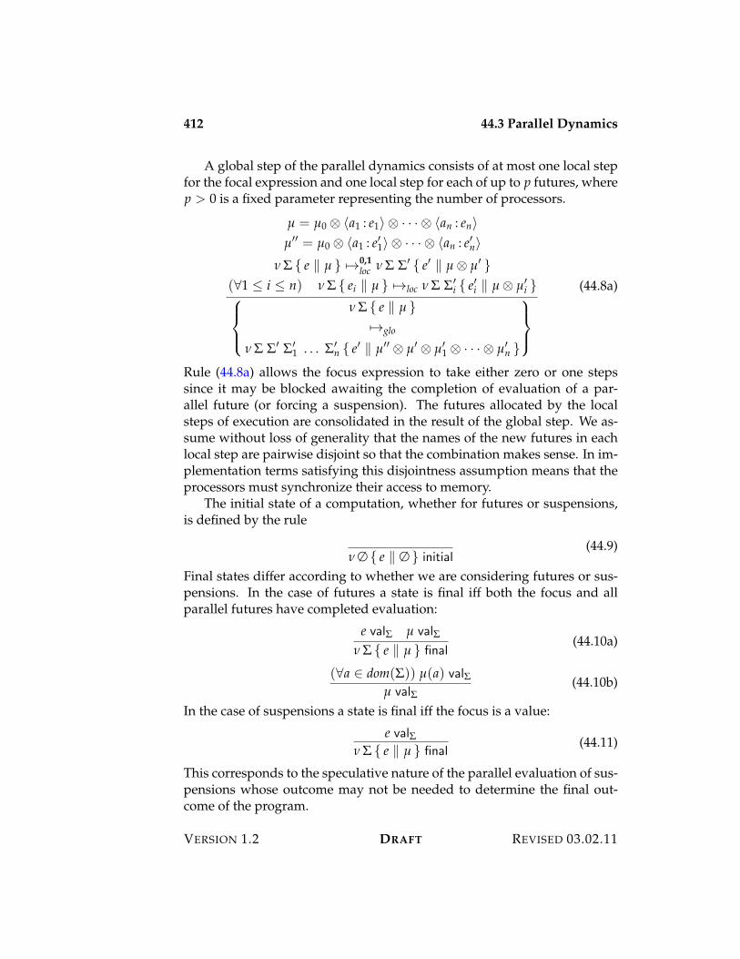
412 44.3 Parallel Dynamics
A global step of the parallel dynamics consists of at most one local stepfor the focal expression and one local step for each of up to p futures, wherep > 0 is a fixed parameter representing the number of processors.
µ = µ0 E ?a1 : e1@ E · · ·E ?an : en@µ%% = µ0 E ?a1 : e%1@ E · · ·E ?an : e%n@
0 $ { e / µ } 530,1loc 0 $ $% { e% / µ E µ% }
(&1 ( i ( n) 0 $ { ei / µ } 53loc 0 $ $%i { e%i / µ E µ%
i },-.
-/
0 $ { e / µ }53glo
0 $ $% $%1 . . . $%
n { e% / µ%% E µ% E µ%1 E · · ·E µ%
n }
0-1
-2
(44.8a)
Rule (44.8a) allows the focus expression to take either zero or one stepssince it may be blocked awaiting the completion of evaluation of a par-allel future (or forcing a suspension). The futures allocated by the localsteps of execution are consolidated in the result of the global step. We as-sume without loss of generality that the names of the new futures in eachlocal step are pairwise disjoint so that the combination makes sense. In im-plementation terms satisfying this disjointness assumption means that theprocessors must synchronize their access to memory.
The initial state of a computation, whether for futures or suspensions,is defined by the rule
0 # { e / # } initial(44.9)
Final states differ according to whether we are considering futures or sus-pensions. In the case of futures a state is final iff both the focus and allparallel futures have completed evaluation:
e val$ µ val$0 $ { e / µ } final
(44.10a)
(&a + dom($)) µ(a) val$µ val$
(44.10b)
In the case of suspensions a state is final iff the focus is a value:
e val$0 $ { e / µ } final
(44.11)
This corresponds to the speculative nature of the parallel evaluation of sus-pensions whose outcome may not be needed to determine the final out-come of the program.
VERSION 1.2 DRAFT REVISED 03.02.11
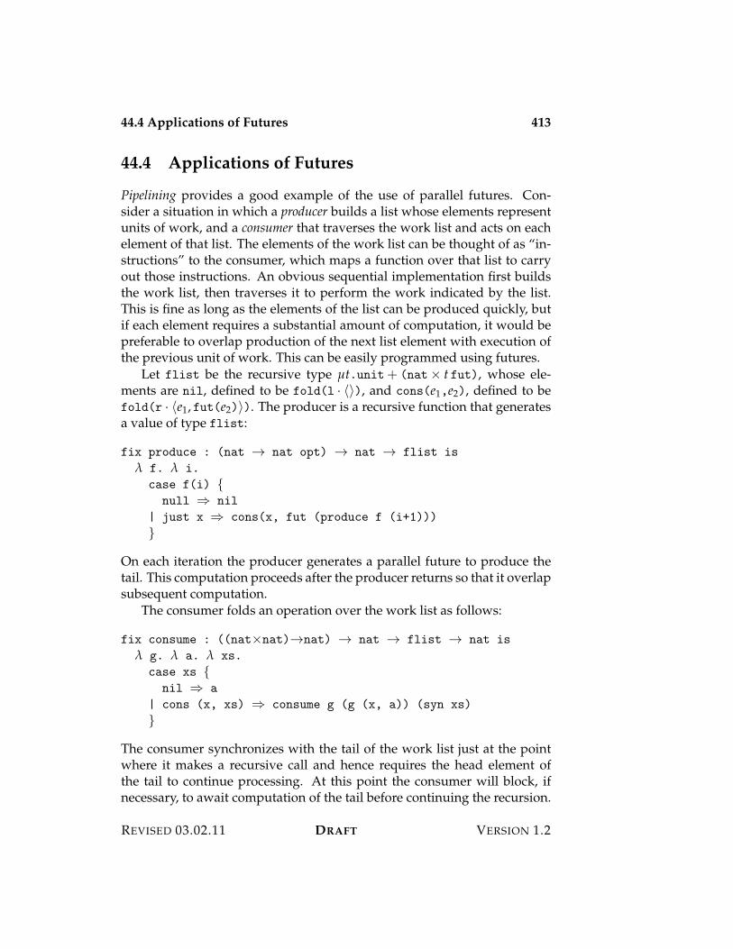
44.4 Applications of Futures 413
44.4 Applications of Futures
Pipelining provides a good example of the use of parallel futures. Con-sider a situation in which a producer builds a list whose elements representunits of work, and a consumer that traverses the work list and acts on eachelement of that list. The elements of the work list can be thought of as “in-structions” to the consumer, which maps a function over that list to carryout those instructions. An obvious sequential implementation first buildsthe work list, then traverses it to perform the work indicated by the list.This is fine as long as the elements of the list can be produced quickly, butif each element requires a substantial amount of computation, it would bepreferable to overlap production of the next list element with execution ofthe previous unit of work. This can be easily programmed using futures.
Let flist be the recursive type µt.unit+ (nat< t fut), whose ele-ments are nil, defined to be fold(l · ?@), and cons(e1,e2), defined to befold(r · ?e1, fut(e2)@). The producer is a recursive function that generatesa value of type flist:
fix produce : (nat 3 nat opt) 3 nat 3 flist is
! f. ! i.
case f(i) {null ; nil
| just x ; cons(x, fut (produce f (i+1)))
}
On each iteration the producer generates a parallel future to produce thetail. This computation proceeds after the producer returns so that it overlapsubsequent computation.
The consumer folds an operation over the work list as follows:
fix consume : ((nat<nat)3nat) 3 nat 3 flist 3 nat is
! g. ! a. ! xs.
case xs {nil ; a
| cons (x, xs) ; consume g (g (x, a)) (syn xs)
}
The consumer synchronizes with the tail of the work list just at the pointwhere it makes a recursive call and hence requires the head element ofthe tail to continue processing. At this point the consumer will block, ifnecessary, to await computation of the tail before continuing the recursion.
REVISED 03.02.11 DRAFT VERSION 1.2
414 44.4 Applications of Futures
Another application of futures is to provide more control over paral-lelism in a language with suspensions. Rather than evaluate suspensionsspeculatively, which is not work efficient, we may instead add futures tothe language in addition to suspensions. One application of futures in sucha setting is called a spark. A spark is a computation that is executed in par-allel with another purely for its effect on suspensions. The spark traverses adata structure, forcing the suspensions within so that their values are com-puted and stored, but otherwise yielding no useful result. The idea is thatthe spark forces the suspensions that will be needed by the main computa-tion, but taking advantage of parallelism in the hope that their values willhave been computed by the time the main computation requires them.
The sequential dynamics of the spark expression spark(e1; e2) is simplyto evaluate e1 before evaluating e2. This is useful in the context of a by-needdynamics for suspensions, since evaluation of e1 will record the values ofsome suspensions in the memo table for subsequent use by the computa-tion e2. The parallel dynamics specifies, in addition, that e1 and e2 are to beevaluated in parallel. The behavior of sparks is captured by the definitionof spark(e1; e2) in terms of futures:
let be fut(e1) in e2.
Evaluation of e1 commences immediately, but its value, if any, is aban-doned. This encoding does not allow for evaluation of e1 to be abandonedas soon as e2 reaches a value, but this scenario is not expected to arise forthe intended mode of use of sparks. The expression e1 should be a quicktraversal that does nothing other than force the suspensions in some datastructure, exiting as soon as this is complete. Presumably this computationtakes less time than it takes for e2 to perform its work before forcing thesuspensions that were forced by e2, otherwise there is little to be gainedfrom the use of sparks in the first place!
As an example, consider the type strm of streams of numbers definedby the recursive type µt.(unit+ (nat< t)) susp. Elements of this typeare suspended computations that, when forced, either signals the end ofstream, or produces a number and another such stream. Suppose that sis such a stream, and assume that we know, for reasons of its construc-tion, that it is finite. We wish to compute map( f)(s) for some functionf , and to overlap this computation with the production of the stream el-ements. We will make use of a function mapforce that forces successiveelements of the input stream, but yields no useful output. The compu-tation spark(mapforce(s); map( f)(s)) forces the elements of the streamin parallel with the computation of map( f)(s), with the intention that all
VERSION 1.2 DRAFT REVISED 03.02.11
44.5 Exercises 415
suspensions in s are forced before their values are required by the maincomputation.
Finally, note that it is easy to encode binary nested parallelism usingfutures. This may be accomplished by defining letpar(e1; e2; x1.x2.e) tostand for the expression
let x%1 be fut(e1) in let x2 be e2 in let x1 be syn(x%1) in e
The order of bindings is important to ensure that evaluation of e2 proceedsin parallel with evaluation of e1. Observe that evaluation of e cannot, in anycase, proceed until both are complete.
44.5 Exercises
REVISED 03.02.11 DRAFT VERSION 1.2

416 44.5 Exercises
VERSION 1.2 DRAFT REVISED 03.02.11

Part XVII
Concurrency

Chapter 45
Process Calculus
So far we have mainly studied the statics and dynamics of programs in iso-lation, without regard to their interaction with the world. But to extend thisanalysis to even the most rudimentary forms of input and output requiresthat we consider external agents that interact with the program. After all,the whole purpose of a computer is to interact with a person!
To extend our investigations to interactive systems, we begin with thestudy of process calculi, which are abstract formalisms that capture the essenceof interaction among independent agents. The development will proceedin stages, starting with simple action models, then extending to interactingconcurrent processes, and finally to synchronous and asynchronous com-munication.
Our presentation differs from that in the literature in several respects.Most significantly, we maintain a distinction between processes and events.The basic form of process is one that awaits the arrival of one of severalevents. Other forms of process include parallel composition and the decla-ration of a communication channel. The basic forms of event are signallingand querying on a channel. Events are combined using a non-deterministicchoice operator that signals the arrival any one of a specified collection ofevents.
45.1 Actions and Events
Our treatment of concurrent interaction is based on the notion of an event,which specifies the actions that a process is prepared to undertake in con-cert with another process. Two processes interact by undertaking two com-plementary actions, which may be thought of as a signal and a query on a
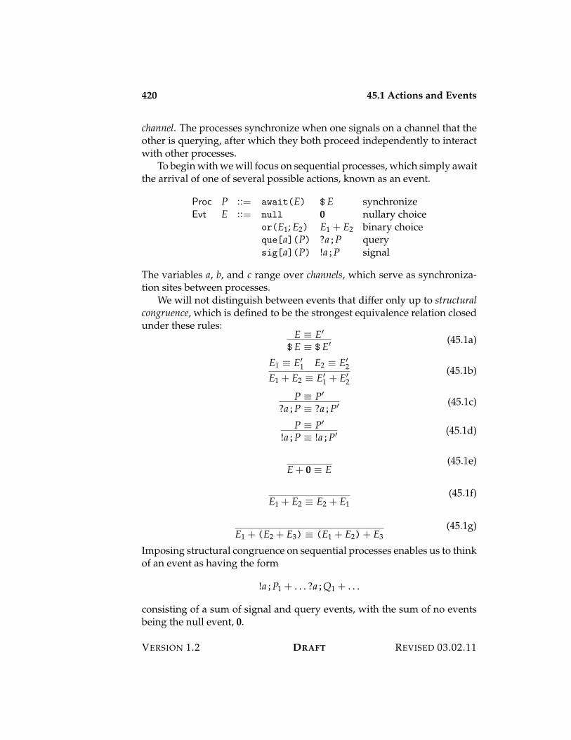
420 45.1 Actions and Events
channel. The processes synchronize when one signals on a channel that theother is querying, after which they both proceed independently to interactwith other processes.
To begin with we will focus on sequential processes, which simply awaitthe arrival of one of several possible actions, known as an event.
Proc P ::= await(E) $ E synchronizeEvt E ::= null 0 nullary choice
or(E1; E2) E1 + E2 binary choiceque[a](P) ?a;P querysig[a](P) !a;P signal
The variables a, b, and c range over channels, which serve as synchroniza-tion sites between processes.
We will not distinguish between events that differ only up to structuralcongruence, which is defined to be the strongest equivalence relation closedunder these rules:
E 9 E%
$ E 9 $ E% (45.1a)
E1 9 E%1 E2 9 E%
2
E1 + E2 9 E%1 + E%
2(45.1b)
P 9 P%
?a;P 9 ?a;P% (45.1c)
P 9 P%
!a;P 9 !a;P% (45.1d)
E + 0 9 E(45.1e)
E1 + E2 9 E2 + E1(45.1f)
E1 + (E2 + E3) 9 (E1 + E2)+ E3(45.1g)
Imposing structural congruence on sequential processes enables us to thinkof an event as having the form
!a;P1 + . . . ?a;Q1 + . . .
consisting of a sum of signal and query events, with the sum of no eventsbeing the null event, 0.
VERSION 1.2 DRAFT REVISED 03.02.11
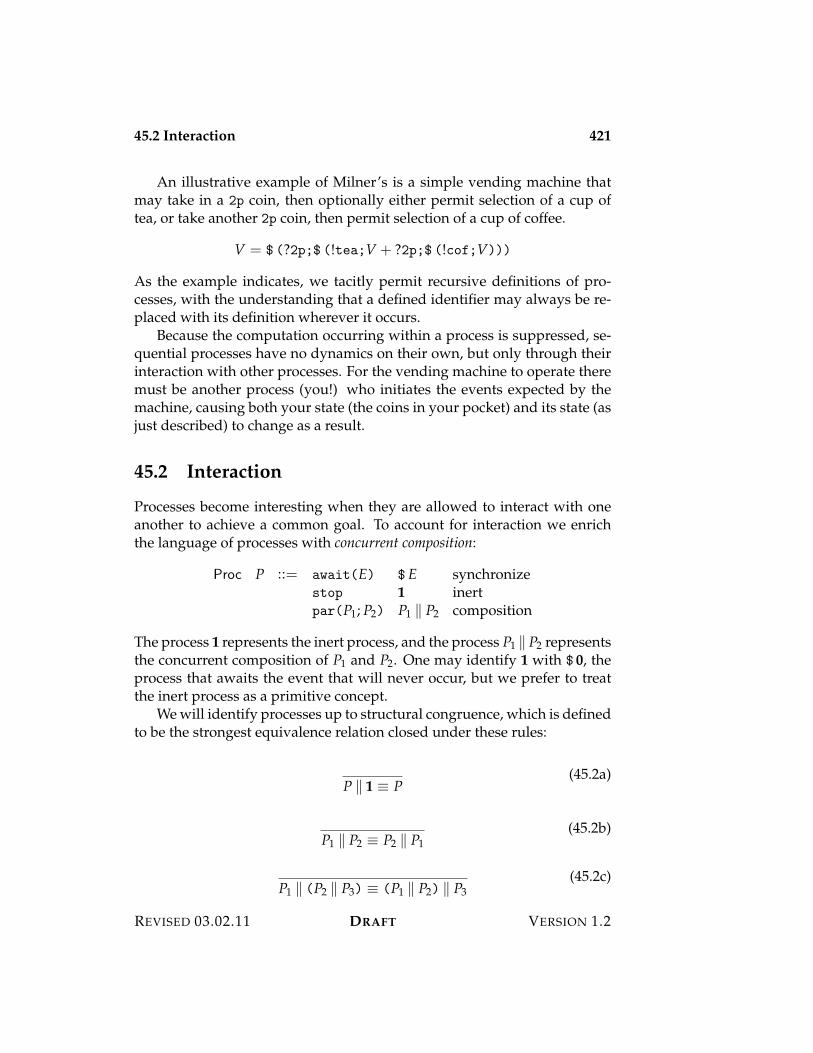
45.2 Interaction 421
An illustrative example of Milner’s is a simple vending machine thatmay take in a 2p coin, then optionally either permit selection of a cup oftea, or take another 2p coin, then permit selection of a cup of coffee.
V = $ (?2p;$ (!tea;V + ?2p;$ (!cof;V)))
As the example indicates, we tacitly permit recursive definitions of pro-cesses, with the understanding that a defined identifier may always be re-placed with its definition wherever it occurs.
Because the computation occurring within a process is suppressed, se-quential processes have no dynamics on their own, but only through theirinteraction with other processes. For the vending machine to operate theremust be another process (you!) who initiates the events expected by themachine, causing both your state (the coins in your pocket) and its state (asjust described) to change as a result.
45.2 Interaction
Processes become interesting when they are allowed to interact with oneanother to achieve a common goal. To account for interaction we enrichthe language of processes with concurrent composition:
Proc P ::= await(E) $ E synchronizestop 1 inertpar(P1; P2) P1 / P2 composition
The process 1 represents the inert process, and the process P1 / P2 representsthe concurrent composition of P1 and P2. One may identify 1 with $ 0, theprocess that awaits the event that will never occur, but we prefer to treatthe inert process as a primitive concept.
We will identify processes up to structural congruence, which is definedto be the strongest equivalence relation closed under these rules:
P / 1 9 P(45.2a)
P1 / P2 9 P2 / P1(45.2b)
P1 / (P2 / P3) 9 (P1 / P2) / P3(45.2c)
REVISED 03.02.11 DRAFT VERSION 1.2
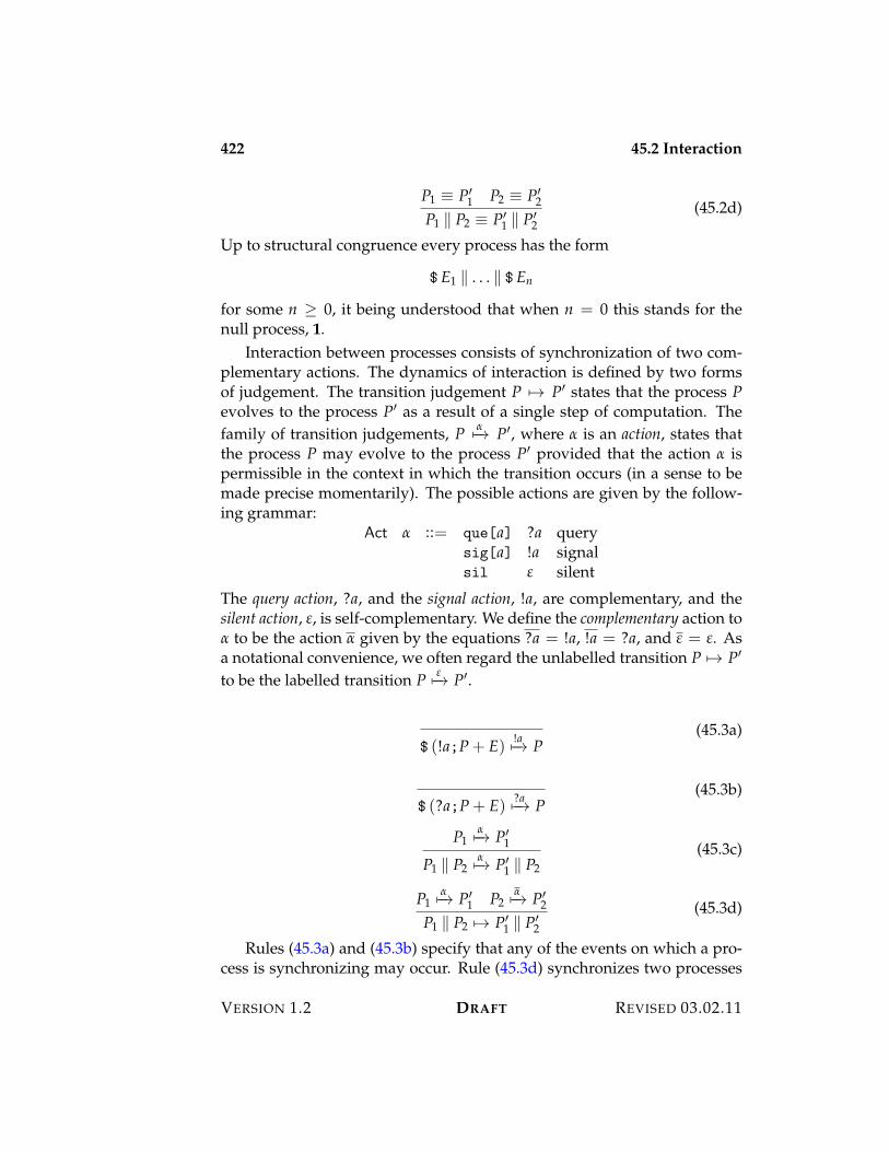
422 45.2 Interaction
P1 9 P%1 P2 9 P%
2
P1 / P2 9 P%1 / P%
2(45.2d)
Up to structural congruence every process has the form
$ E1 / . . . / $ En
for some n 7 0, it being understood that when n = 0 this stands for thenull process, 1.
Interaction between processes consists of synchronization of two com-plementary actions. The dynamics of interaction is defined by two formsof judgement. The transition judgement P 53 P% states that the process Pevolves to the process P% as a result of a single step of computation. Thefamily of transition judgements, P $5$3 P%, where $ is an action, states thatthe process P may evolve to the process P% provided that the action $ ispermissible in the context in which the transition occurs (in a sense to bemade precise momentarily). The possible actions are given by the follow-ing grammar:
Act $ ::= que[a] ?a querysig[a] !a signalsil 1 silent
The query action, ?a, and the signal action, !a, are complementary, and thesilent action, 1, is self-complementary. We define the complementary action to$ to be the action $ given by the equations ?a = !a, !a = ?a, and 1 = 1. Asa notational convenience, we often regard the unlabelled transition P 53 P%
to be the labelled transition P 15$3 P%.
$ (!a;P + E) !a5$3 P(45.3a)
$ (?a;P + E) ?a5$3 P(45.3b)
P1$5$3 P%
1
P1 / P2$5$3 P%
1 / P2(45.3c)
P1$5$3 P%
1 P2$5$3 P%
2
P1 / P2 53 P%1 / P%
2
(45.3d)
Rules (45.3a) and (45.3b) specify that any of the events on which a pro-cess is synchronizing may occur. Rule (45.3d) synchronizes two processes
VERSION 1.2 DRAFT REVISED 03.02.11
45.3 Replication 423
that take complementary actions. (When $ is the silent action, Rule (45.3d)is derivable by two applications of Rule (45.3c).)
As an example, let us consider the interaction of the vending machine,V, with the user process, U, defined as follows:
U = $ !2p;$ !2p;$ ?cof;1.
Here is a trace of the interaction between V and U:
V / U 53 $ !tea;V + ?2p;$ !cof;V / $ !2p;$ ?cof;153 $ !cof;V / $ ?cof;153 V
These steps are justified, respectively, by the following pairs of labelledtransitions:
U!2p5$$3 U% = $ !2p;$ ?cof;1
V?2p5$$3 V % = $ (!tea;V + ?2p;$ !cof;V)
U% !2p5$$3 U%% = $ ?cof;1
V % ?2p5$$3 V %% = $ !cof;V
U%% ?cof5$$$3 1
V %% !cof5$$3 V
We have suppressed uses of structural congruence in the above derivationsto avoid clutter, but it is important to see its role in managing the non-deterministic choice of events by a process.
45.3 Replication
Some presentations of process calculi forego reliance on defining equationsfor processes in favor of a replication construct, which we write 1 P. Thisprocess stands for as many concurrently executing copies of P as one mayrequire, which may be modeled by the structural congruence
1 P 9 P / 1 P. (45.4)
REVISED 03.02.11 DRAFT VERSION 1.2
424 45.3 Replication
Taking this as a principle of structural congruence hides the overhead ofprocess creation, and gives no hint as to how often it can or should be ap-plied. One could alternatively build replication into the dynamics to modelthe details of replication more closely:
1 P 53 P / 1 P. (45.5)
Since the application of this rule is unconstrained, it may be applied at anytime to effect a new copy of the replicated process P.
So far we have been using recursive process definitions to define pro-cesses that interact repeatedly according to some protocol. Rather than takerecursive definition as a primitive notion, we may instead use replicationto model repetition. This may be achieved by introducing an “activator”process that is contacted to effect the replication. Consider the recursivedefinition X = P(X), where P is a process expression involving occur-rences of the process variable, X, to refer to itself. This may be simulatedby defining the activator process
A = 1 $ (?a;P($ (!a;1))),
in which we have replaced occurrences of X within P by an initiator processthat signals the event a to the activator. Observe that the activator, A, isstructurally congruent to the process A% / A, where A% is the process
$ (?a;P($ (!a;1))).
To start process P we concurrently compose the activator, A, with an initia-tor process, $ (!a;1). Observe that
A / $ (!a;1) 53 A / P(!a;1),
which starts the process P while maintaining a running copy of the activa-tor, A.
As an example, let us consider Milner’s vending machine written usingreplication, rather than using recursive process definition:
V0 = $ (!v;1) (45.6)V1 = 1 $ (?v;V2) (45.7)V2 = $ (?2p;$ (!tea;V0 + ?2p;$ (!cof;V0))) (45.8)
The process V1 is a replicated server that awaits a signal on channel v tocreate another instance of the vending machine. The recursive calls are
VERSION 1.2 DRAFT REVISED 03.02.11
45.4 Allocating Channels 425
replaced by signals along v to re-start the machine. The original machine,V, is simulated by the concurrent composition V0 / V1.
This example motivates a restriction on replication that avoids the in-determinacy inherent in accounting for it either as part of structural con-gruence (Rule (45.4)) or as a computation step (Rule (45.5)). Rather thantake replication as a primitive notion, we may instead take replicated syn-chronization as a primitive notion governed by the following rules:
1 $ (!a;P + E) !a5$3 P / 1 $ (!a;P + E)(45.9a)
1 $ (?a;P + E) ?a5$3 P / 1 $ (?a;P + E)(45.9b)
The process 1 $ (E) is to be regarded not as a composition of replicationand synchronization, but as the inseparable combination of these two con-structs. The advantage is that the replication occurs only as needed, pre-cisely when a synchronization with another process is possible. This avoidsthe need to “guess”, either by structural congruence or an explicit step,when to replicate a process.
45.4 Allocating Channels
It is often useful (particularly once we have introduce inter-process com-munication) to introduce new channels within a process, rather than as-sume that all channels of interaction are given a priori. To allow for this, thesyntax of processes is enriched with a channel declaration primitive:
Proc P ::= new(a.P) 0 a.P new channel
The channel, a, is bound within the process P, and hence may be renamedat will (avoiding conflicts) within P. To simplify notation we sometimeswrite 0 a1, . . . , ak.P for the iterated declaration 0 a1.. . . 0 ak.P.
Structural congruence is extended with the following rules:
P =$ P%
P 9 P% (45.10a)
P 9 P%
0 a.P 9 0 a.P% (45.10b)
REVISED 03.02.11 DRAFT VERSION 1.2
426 45.4 Allocating Channels
a /+ P2
(0 a.P1) / P2 9 0 a.(P1 / P2)(45.10c)
(a /+ P)0 a.P 9 P
(45.10d)
The last rule, called scope extrusion, will be important in the treatment ofcommunication in Section 45.5 on page 428. Since we identify processes upto renaming of bound names, the requirement that a /+ P2 in Rule (45.10c)may always be met by choosing the name a suitably. Rule (45.10d) statesthat channels may be de-allocated once they are no longer in use.
To account for the scopes of names (and to prepare for later generaliza-tions) it is useful to introduce a static semantics for processes that ensuresthat names are properly scoped. A signature, $, is, for the time being, afinite set of channels. The judgement )$ P proc states that a process, P, iswell-formed relative to the channels declared in the signature, $.
)$ 1 proc(45.11a)
)$ P1 proc )$ P2 proc
)$ P1 / P2 proc(45.11b)
)$ E event)$ $ E proc
(45.11c)
)$,a P proc
)$ 0 a.P proc(45.11d)
The foregoing rules make use of an auxiliary judgement, )$ E event, statingthat E is a well-formed event relative to $.
)$ 0 event(45.12a)
)$,a P proc
)$,a ?a;P event(45.12b)
)$,a P proc
)$,a !a;P event(45.12c)
)$ E1 event )$ E2 event)$ E1 + E2 event
(45.12d)
VERSION 1.2 DRAFT REVISED 03.02.11
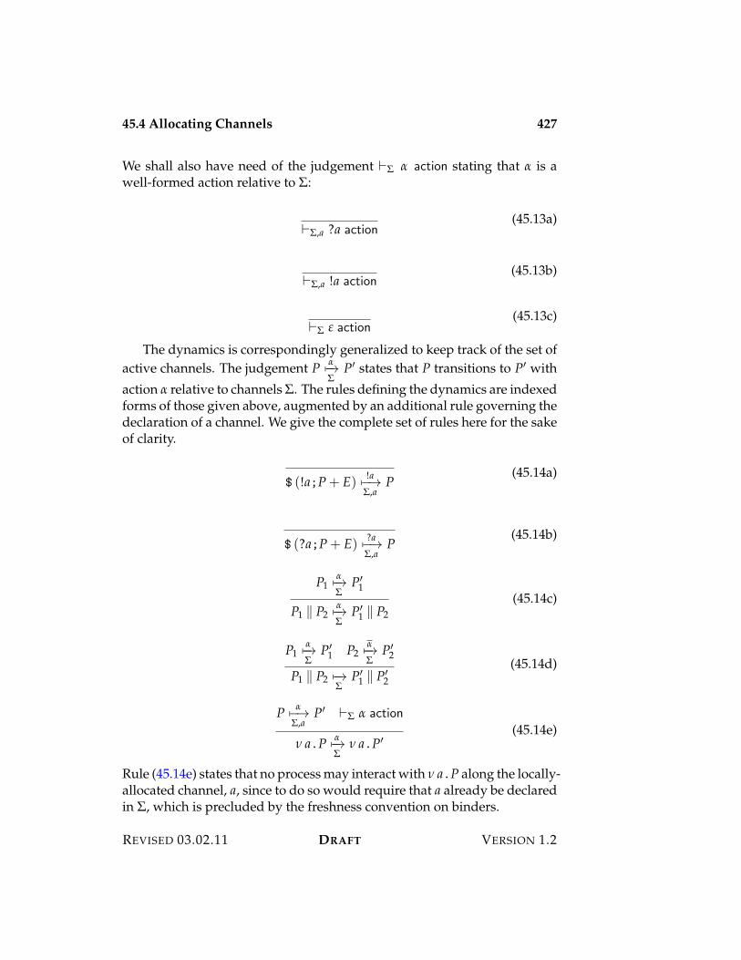
45.4 Allocating Channels 427
We shall also have need of the judgement )$ $ action stating that $ is awell-formed action relative to $:
)$,a ?a action(45.13a)
)$,a !a action(45.13b)
)$ 1 action(45.13c)
The dynamics is correspondingly generalized to keep track of the set ofactive channels. The judgement P $5$3
$P% states that P transitions to P% with
action $ relative to channels $. The rules defining the dynamics are indexedforms of those given above, augmented by an additional rule governing thedeclaration of a channel. We give the complete set of rules here for the sakeof clarity.
$ (!a;P + E) !a5$3$,a
P(45.14a)
$ (?a;P + E) ?a5$3$,a
P(45.14b)
P1$5$3$
P%1
P1 / P2$5$3$
P%1 / P2
(45.14c)
P1$5$3$
P%1 P2
$5$3$
P%2
P1 / P2 5$3$
P%1 / P%
2
(45.14d)
P $5$3$,a
P% )$ $ action
0 a.P $5$3$
0 a.P%(45.14e)
Rule (45.14e) states that no process may interact with 0 a.P along the locally-allocated channel, a, since to do so would require that a already be declaredin $, which is precluded by the freshness convention on binders.
REVISED 03.02.11 DRAFT VERSION 1.2
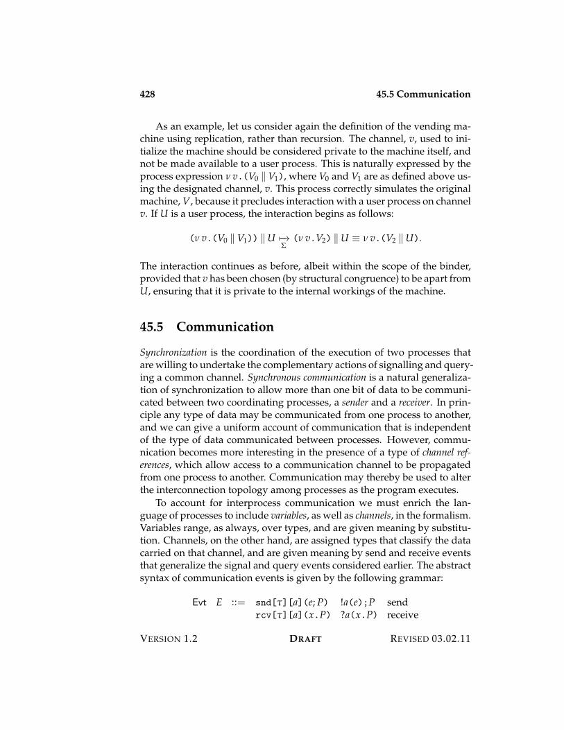
428 45.5 Communication
As an example, let us consider again the definition of the vending ma-chine using replication, rather than recursion. The channel, v, used to ini-tialize the machine should be considered private to the machine itself, andnot be made available to a user process. This is naturally expressed by theprocess expression 0 v.(V0 / V1), where V0 and V1 are as defined above us-ing the designated channel, v. This process correctly simulates the originalmachine, V, because it precludes interaction with a user process on channelv. If U is a user process, the interaction begins as follows:
(0 v.(V0 / V1)) / U 5$3$
(0 v.V2) / U 9 0 v.(V2 / U).
The interaction continues as before, albeit within the scope of the binder,provided that v has been chosen (by structural congruence) to be apart fromU, ensuring that it is private to the internal workings of the machine.
45.5 Communication
Synchronization is the coordination of the execution of two processes thatare willing to undertake the complementary actions of signalling and query-ing a common channel. Synchronous communication is a natural generaliza-tion of synchronization to allow more than one bit of data to be communi-cated between two coordinating processes, a sender and a receiver. In prin-ciple any type of data may be communicated from one process to another,and we can give a uniform account of communication that is independentof the type of data communicated between processes. However, commu-nication becomes more interesting in the presence of a type of channel ref-erences, which allow access to a communication channel to be propagatedfrom one process to another. Communication may thereby be used to alterthe interconnection topology among processes as the program executes.
To account for interprocess communication we must enrich the lan-guage of processes to include variables, as well as channels, in the formalism.Variables range, as always, over types, and are given meaning by substitu-tion. Channels, on the other hand, are assigned types that classify the datacarried on that channel, and are given meaning by send and receive eventsthat generalize the signal and query events considered earlier. The abstractsyntax of communication events is given by the following grammar:
Evt E ::= snd["][a](e; P) !a(e);P sendrcv["][a](x.P) ?a(x.P) receive
VERSION 1.2 DRAFT REVISED 03.02.11
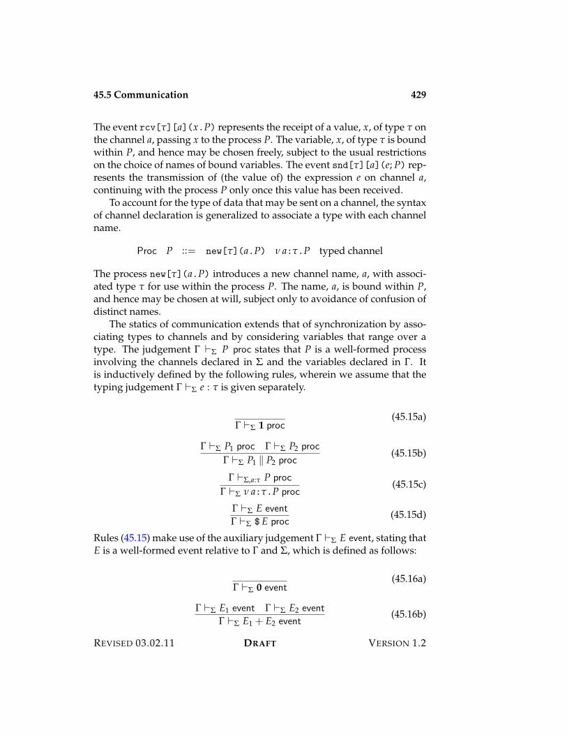
45.5 Communication 429
The event rcv["][a](x.P) represents the receipt of a value, x, of type " onthe channel a, passing x to the process P. The variable, x, of type " is boundwithin P, and hence may be chosen freely, subject to the usual restrictionson the choice of names of bound variables. The event snd["][a](e; P) rep-resents the transmission of (the value of) the expression e on channel a,continuing with the process P only once this value has been received.
To account for the type of data that may be sent on a channel, the syntaxof channel declaration is generalized to associate a type with each channelname.
Proc P ::= new["](a.P) 0 a:".P typed channel
The process new["](a.P) introduces a new channel name, a, with associ-ated type " for use within the process P. The name, a, is bound within P,and hence may be chosen at will, subject only to avoidance of confusion ofdistinct names.
The statics of communication extends that of synchronization by asso-ciating types to channels and by considering variables that range over atype. The judgement ! )$ P proc states that P is a well-formed processinvolving the channels declared in $ and the variables declared in !. Itis inductively defined by the following rules, wherein we assume that thetyping judgement ! )$ e : " is given separately.
! )$ 1 proc(45.15a)
! )$ P1 proc ! )$ P2 proc
! )$ P1 / P2 proc(45.15b)
! )$,a:" P proc
! )$ 0 a:".P proc(45.15c)
! )$ E event! )$ $ E proc
(45.15d)
Rules (45.15) make use of the auxiliary judgement ! )$ E event, stating thatE is a well-formed event relative to ! and $, which is defined as follows:
! )$ 0 event(45.16a)
! )$ E1 event ! )$ E2 event! )$ E1 + E2 event
(45.16b)
REVISED 03.02.11 DRAFT VERSION 1.2
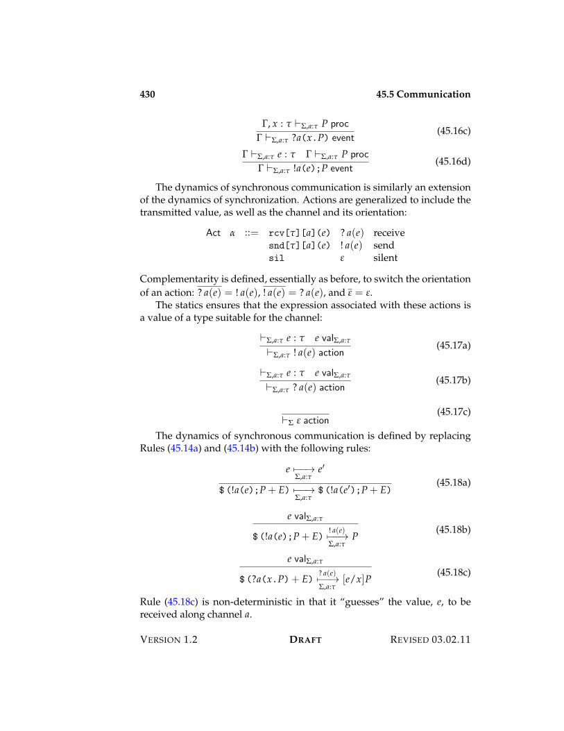
430 45.5 Communication
!, x : " )$,a:" P proc
! )$,a:" ?a(x.P) event(45.16c)
! )$,a:" e : " ! )$,a:" P proc
! )$,a:" !a(e);P event(45.16d)
The dynamics of synchronous communication is similarly an extensionof the dynamics of synchronization. Actions are generalized to include thetransmitted value, as well as the channel and its orientation:
Act $ ::= rcv["][a](e) ? a(e) receivesnd["][a](e) ! a(e) sendsil 1 silent
Complementarity is defined, essentially as before, to switch the orientationof an action: ? a(e) = ! a(e), ! a(e) = ? a(e), and 1 = 1.
The statics ensures that the expression associated with these actions isa value of a type suitable for the channel:
)$,a:" e : " e val$,a:"
)$,a:" ! a(e) action(45.17a)
)$,a:" e : " e val$,a:"
)$,a:" ? a(e) action(45.17b)
)$ 1 action(45.17c)
The dynamics of synchronous communication is defined by replacingRules (45.14a) and (45.14b) with the following rules:
e 5$$3$,a:"
e%
$ (!a(e);P + E) 5$$3$,a:"
$ (!a(e%);P + E)(45.18a)
e val$,a:"
$ (!a(e);P + E)! a(e)5$$3$,a:"
P(45.18b)
e val$,a:"
$ (?a(x.P)+ E)? a(e)5$$3$,a:"
[e/x]P(45.18c)
Rule (45.18c) is non-deterministic in that it “guesses” the value, e, to bereceived along channel a.
VERSION 1.2 DRAFT REVISED 03.02.11
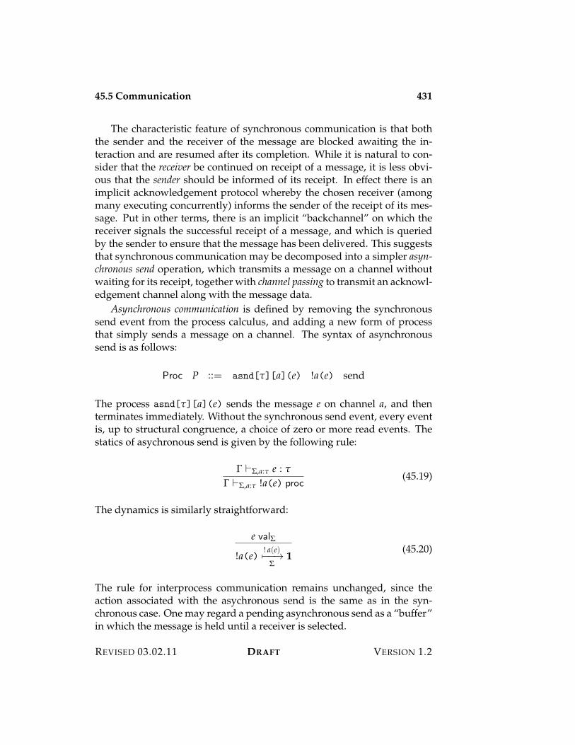
45.5 Communication 431
The characteristic feature of synchronous communication is that boththe sender and the receiver of the message are blocked awaiting the in-teraction and are resumed after its completion. While it is natural to con-sider that the receiver be continued on receipt of a message, it is less obvi-ous that the sender should be informed of its receipt. In effect there is animplicit acknowledgement protocol whereby the chosen receiver (amongmany executing concurrently) informs the sender of the receipt of its mes-sage. Put in other terms, there is an implicit “backchannel” on which thereceiver signals the successful receipt of a message, and which is queriedby the sender to ensure that the message has been delivered. This suggeststhat synchronous communication may be decomposed into a simpler asyn-chronous send operation, which transmits a message on a channel withoutwaiting for its receipt, together with channel passing to transmit an acknowl-edgement channel along with the message data.
Asynchronous communication is defined by removing the synchronoussend event from the process calculus, and adding a new form of processthat simply sends a message on a channel. The syntax of asynchronoussend is as follows:
Proc P ::= asnd["][a](e) !a(e) send
The process asnd["][a](e) sends the message e on channel a, and thenterminates immediately. Without the synchronous send event, every eventis, up to structural congruence, a choice of zero or more read events. Thestatics of asychronous send is given by the following rule:
! )$,a:" e : "
! )$,a:" !a(e) proc(45.19)
The dynamics is similarly straightforward:
e val$
!a(e)! a(e)5$$3
$1
(45.20)
The rule for interprocess communication remains unchanged, since theaction associated with the asychronous send is the same as in the syn-chronous case. One may regard a pending asynchronous send as a “buffer”in which the message is held until a receiver is selected.
REVISED 03.02.11 DRAFT VERSION 1.2
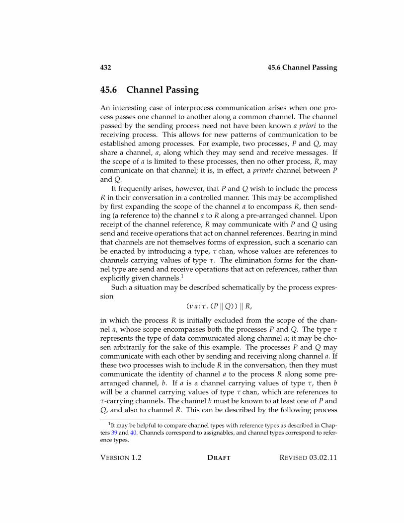
432 45.6 Channel Passing
45.6 Channel Passing
An interesting case of interprocess communication arises when one pro-cess passes one channel to another along a common channel. The channelpassed by the sending process need not have been known a priori to thereceiving process. This allows for new patterns of communication to beestablished among processes. For example, two processes, P and Q, mayshare a channel, a, along which they may send and receive messages. Ifthe scope of a is limited to these processes, then no other process, R, maycommunicate on that channel; it is, in effect, a private channel between Pand Q.
It frequently arises, however, that P and Q wish to include the processR in their conversation in a controlled manner. This may be accomplishedby first expanding the scope of the channel a to encompass R, then send-ing (a reference to) the channel a to R along a pre-arranged channel. Uponreceipt of the channel reference, R may communicate with P and Q usingsend and receive operations that act on channel references. Bearing in mindthat channels are not themselves forms of expression, such a scenario canbe enacted by introducing a type, " chan, whose values are references tochannels carrying values of type ". The elimination forms for the chan-nel type are send and receive operations that act on references, rather thanexplicitly given channels.1
Such a situation may be described schematically by the process expres-sion
(0 a:".(P / Q)) / R,
in which the process R is initially excluded from the scope of the chan-nel a, whose scope encompasses both the processes P and Q. The type "represents the type of data communicated along channel a; it may be cho-sen arbitrarily for the sake of this example. The processes P and Q maycommunicate with each other by sending and receiving along channel a. Ifthese two processes wish to include R in the conversation, then they mustcommunicate the identity of channel a to the process R along some pre-arranged channel, b. If a is a channel carrying values of type ", then bwill be a channel carrying values of type " chan, which are references to"-carrying channels. The channel b must be known to at least one of P andQ, and also to channel R. This can be described by the following process
1It may be helpful to compare channel types with reference types as described in Chap-ters 39 and 40. Channels correspond to assignables, and channel types correspond to refer-ence types.
VERSION 1.2 DRAFT REVISED 03.02.11
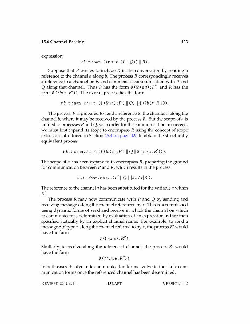
45.6 Channel Passing 433
expression:0 b:" chan.((0 a:".(P / Q)) / R).
Suppose that P wishes to include R in the conversation by sending areference to the channel a along b. The process R correspondingly receivesa reference to a channel on b, and commences communication with P andQ along that channel. Thus P has the form $ (!b(& a);P%) and R has theform $ (?b(x.R%)). The overall process has the form
0 b:" chan.(0 a:".($ (!b(a);P%) / Q) / $ (?b(x.R%))).
The process P is prepared to send a reference to the channel a along thechannel b, where it may be received by the process R. But the scope of a islimited to processes P and Q, so in order for the communication to succeed,we must first expand its scope to encompass R using the concept of scopeextrusion introduced in Section 45.4 on page 425 to obtain the structurallyequivalent process
0 b:" chan.0 a:".($ (!b(a);P%) / Q / $ (?b(x.R%))).
The scope of a has been expanded to encompass R, preparing the groundfor communication between P and R, which results in the process
0 b:" chan.0 a:".(P% / Q / [& a/x]R%).
The reference to the channel a has been substituted for the variable x withinR%.
The process R may now communicate with P and Q by sending andreceiving messages along the channel referenced by x. This is accomplishedusing dynamic forms of send and receive in which the channel on whichto communicate is determined by evaluation of an expression, rather thanspecified statically by an explicit channel name. For example, to send amessage e of type " along the channel referred to by x, the process R% wouldhave the form
$ (!!(x; e);R%%).
Similarly, to receive along the referenced channel, the process R% wouldhave the form
$ (??(x; y.R%%)).
In both cases the dynamic communication forms evolve to the static com-munication forms once the referenced channel has been determined.
REVISED 03.02.11 DRAFT VERSION 1.2
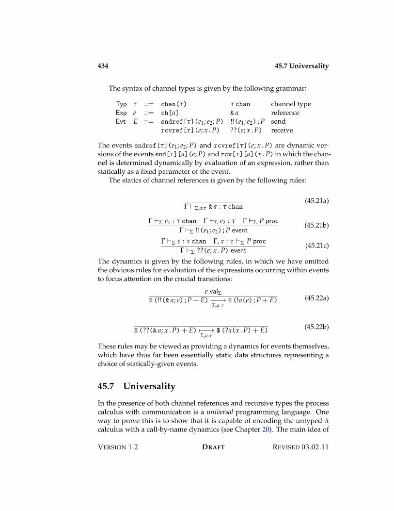
434 45.7 Universality
The syntax of channel types is given by the following grammar:
Typ " ::= chan(") " chan channel typeExp e ::= ch[a] & a referenceEvt E ::= sndref["](e1; e2; P) !!(e1; e2);P send
rcvref["](e; x.P) ??(e; x.P) receive
The events sndref["](e1; e2; P) and rcvref["](e; x.P) are dynamic ver-sions of the events snd["][a](e; P) and rcv["][a](x.P) in which the chan-nel is determined dynamically by evaluation of an expression, rather thanstatically as a fixed parameter of the event.
The statics of channel references is given by the following rules:
! )$,a:" & a : " chan(45.21a)
! )$ e1 : " chan ! )$ e2 : " ! )$ P proc! )$ !!(e1; e2);P event
(45.21b)
! )$ e : " chan !, x : " )$ P proc! )$ ??(e; x.P) event
(45.21c)
The dynamics is given by the following rules, in which we have omittedthe obvious rules for evaluation of the expressions occurring within eventsto focus attention on the crucial transitions:
e val$$ (!!(& a; e);P + E) 5$$3
$,a:"$ (!a(e);P + E) (45.22a)
$ (??(& a; x.P)+ E) 5$$3$,a:"
$ (?a(x.P)+ E) (45.22b)
These rules may be viewed as providing a dynamics for events themselves,which have thus far been essentially static data structures representing achoice of statically-given events.
45.7 Universality
In the presence of both channel references and recursive types the processcalculus with communication is a universal programming language. Oneway to prove this is to show that it is capable of encoding the untyped !calculus with a call-by-name dynamics (see Chapter 20). The main idea of
VERSION 1.2 DRAFT REVISED 03.02.11
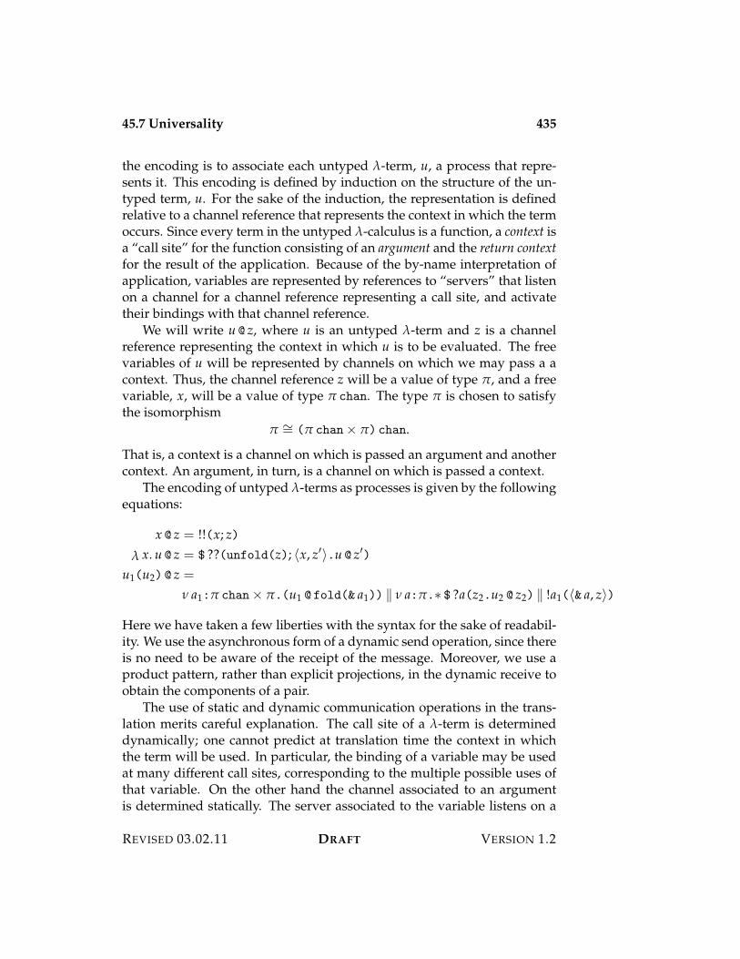
45.7 Universality 435
the encoding is to associate each untyped !-term, u, a process that repre-sents it. This encoding is defined by induction on the structure of the un-typed term, u. For the sake of the induction, the representation is definedrelative to a channel reference that represents the context in which the termoccurs. Since every term in the untyped !-calculus is a function, a context isa “call site” for the function consisting of an argument and the return contextfor the result of the application. Because of the by-name interpretation ofapplication, variables are represented by references to “servers” that listenon a channel for a channel reference representing a call site, and activatetheir bindings with that channel reference.
We will write u @ z, where u is an untyped !-term and z is a channelreference representing the context in which u is to be evaluated. The freevariables of u will be represented by channels on which we may pass a acontext. Thus, the channel reference z will be a value of type #, and a freevariable, x, will be a value of type # chan. The type # is chosen to satisfythe isomorphism
# I= (# chan< #) chan.
That is, a context is a channel on which is passed an argument and anothercontext. An argument, in turn, is a channel on which is passed a context.
The encoding of untyped !-terms as processes is given by the followingequations:
x @ z = !!(x; z)! x. u @ z = $ ??(unfold(z); ?x, z%@.u @ z%)
u1(u2) @ z =
0 a1:# chan< #.(u1 @ fold(& a1)) / 0 a:#.1 $ ?a(z2.u2 @ z2) / !a1(?& a, z@)
Here we have taken a few liberties with the syntax for the sake of readabil-ity. We use the asynchronous form of a dynamic send operation, since thereis no need to be aware of the receipt of the message. Moreover, we use aproduct pattern, rather than explicit projections, in the dynamic receive toobtain the components of a pair.
The use of static and dynamic communication operations in the trans-lation merits careful explanation. The call site of a !-term is determineddynamically; one cannot predict at translation time the context in whichthe term will be used. In particular, the binding of a variable may be usedat many different call sites, corresponding to the multiple possible uses ofthat variable. On the other hand the channel associated to an argumentis determined statically. The server associated to the variable listens on a
REVISED 03.02.11 DRAFT VERSION 1.2
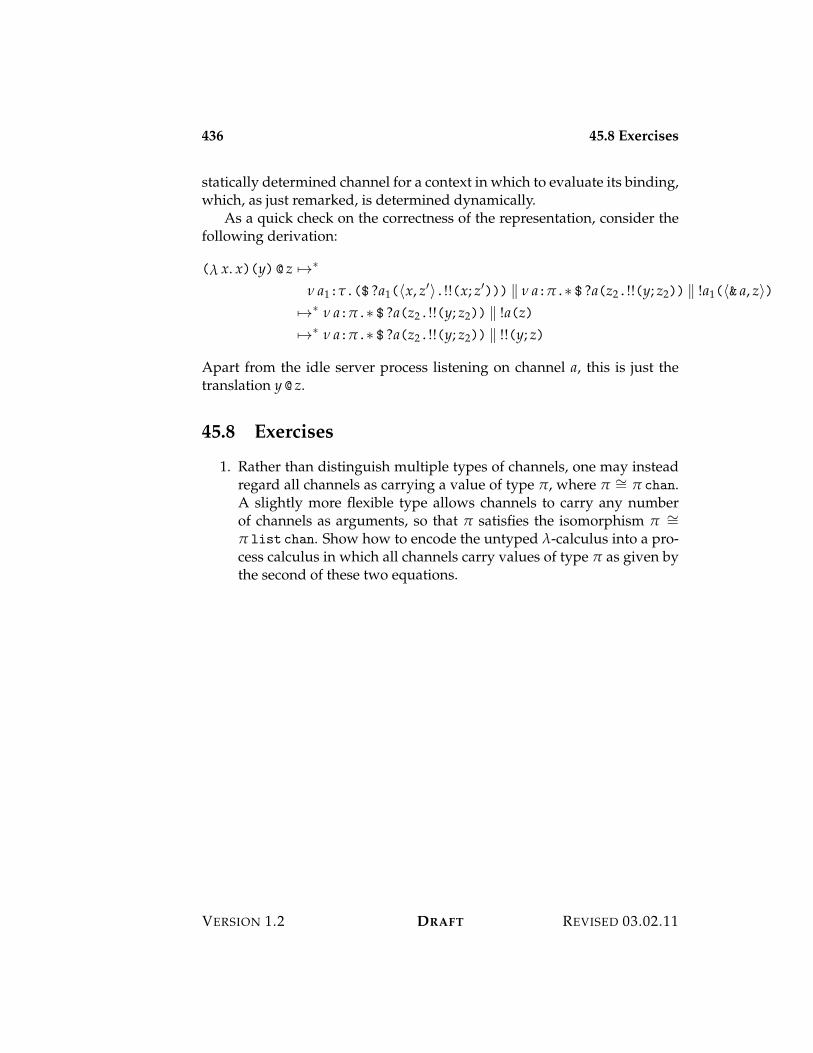
436 45.8 Exercises
statically determined channel for a context in which to evaluate its binding,which, as just remarked, is determined dynamically.
As a quick check on the correctness of the representation, consider thefollowing derivation:
(! x. x)(y) @ z 531
0 a1:".($ ?a1(?x, z%@.!!(x; z%))) / 0 a:#.1 $ ?a(z2.!!(y; z2)) / !a1(?& a, z@)531 0 a:#.1 $ ?a(z2.!!(y; z2)) / !a(z)531 0 a:#.1 $ ?a(z2.!!(y; z2)) / !!(y; z)
Apart from the idle server process listening on channel a, this is just thetranslation y @ z.
45.8 Exercises
1. Rather than distinguish multiple types of channels, one may insteadregard all channels as carrying a value of type #, where # I= # chan.A slightly more flexible type allows channels to carry any numberof channels as arguments, so that # satisfies the isomorphism # I=# list chan. Show how to encode the untyped !-calculus into a pro-cess calculus in which all channels carry values of type # as given bythe second of these two equations.
VERSION 1.2 DRAFT REVISED 03.02.11
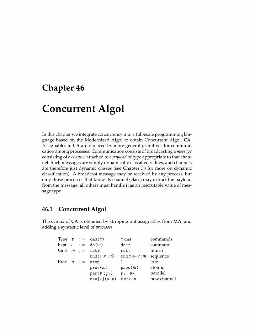
Chapter 46
Concurrent Algol
In this chapter we integrate concurrency into a full-scale programming lan-guage based on the Modernized Algol to obtain Concurrent Algol, CA.Assignables in CA are replaced by more general primitives for communi-cation among processes. Communication consists of broadcasting a messageconsisting of a channel attached to a payload of type appropriate to that chan-nel. Such messages are simply dynamically classified values, and channelsare therefore just dynamic classes (see Chapter 38 for more on dynamicclassification). A broadcast message may be received by any process, butonly those processes that know its channel (class) may extract the payloadfrom the message; all others must handle it as an inscrutable value of mes-sage type.
46.1 Concurrent Algol
The syntax of CA is obtained by stripping out assignables from MA, andadding a syntactic level of processes:
Type " ::= cmd(") " cmd commandsExpr e ::= do(m) dom commandCmd m ::= ret e ret e return
bnd(e; x.m) bnd x 2 e ; m sequenceProc p ::= stop 1 idle
proc(m) proc(m) atomicpar(p1; p2) p1 / p2 parallelnew["](a.p) 0 a:".p new channel
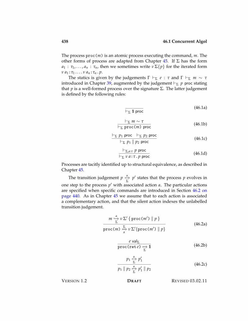
438 46.1 Concurrent Algol
The process proc(m) is an atomic process executing the command, m. Theother forms of process are adapted from Chapter 45. If $ has the forma1 : "1, . . . , an : "n, then we sometimes write 0 ${p} for the iterated form0 a1:"1.. . . 0 an:"n.p.
The statics is given by the judgements ! )$ e : " and ! )$ m I "introduced in Chapter 39, augmented by the judgement )$ p proc statingthat p is a well-formed process over the signature $. The latter judgementis defined by the following rules:
)$ 1 proc(46.1a)
)$ m I ")$ proc(m) proc
(46.1b)
)$ p1 proc )$ p2 proc
)$ p1 / p2 proc(46.1c)
)$,a:" p proc
)$ 0 a:".p proc(46.1d)
Processes are tacitly identified up to structural equivalence, as described inChapter 45.
The transition judgement p $5$3$
p% states that the process p evolves in
one step to the process p% with associated action $. The particular actionsare specified when specific commands are introduced in Section 46.2 onpage 440. As in Chapter 45 we assume that to each action is associateda complementary action, and that the silent action indexes the unlabelledtransition judgement.
m$%$3
$0 $% { proc(m%) / p }
proc(m)$5$3$
0 $%{proc(m%) / p}(46.2a)
e val$proc(ret e) 5$3
$1 (46.2b)
p1$5$3$
p%1
p1 / p2$5$3$
p%1 / p2(46.2c)
VERSION 1.2 DRAFT REVISED 03.02.11
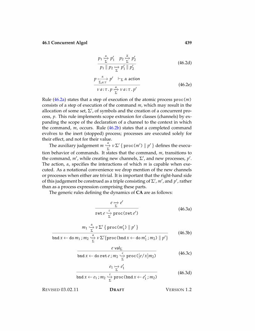
46.1 Concurrent Algol 439
p1$5$3$
p%1 p2$5$3$
p%2
p1 / p2 5$3$
p%1 / p%2(46.2d)
p $5$$3$,$:"
p% )$ $ action
0 a:".p $5$3$
0 a:".p%(46.2e)
Rule (46.2a) states that a step of execution of the atomic process proc(m)
consists of a step of execution of the command m, which may result in theallocation of some set, $%, of symbols and the creation of a concurrent pro-cess, p. This rule implements scope extrusion for classes (channels) by ex-panding the scope of the declaration of a channel to the context in whichthe command, m, occurs. Rule (46.2b) states that a completed commandevolves to the inert (stopped) process; processes are executed solely fortheir effect, and not for their value.
The auxiliary judgement m$%$3
$0 $% { proc(m%) / p% } defines the execu-
tion behavior of commands. It states that the command, m, transitions tothe command, m%, while creating new channels, $%, and new processes, p%.The action, $, specifies the interactions of which m is capable when exe-cuted. As a notational convenience we drop mention of the new channelsor processes when either are trivial. It is important that the right-hand sideof this judgement be construed as a triple consisting of $%, m%, and p%, ratherthan as a process expression comprising these parts.
The generic rules defining the dynamics of CA are as follows:
e 5$3$
e%
ret e1
%$3$
proc(ret e%)(46.3a)
m1$%$3
$0 $% { proc(m%
1) / p% }
bnd x 2 dom1 ; m2$%$3
$0 $%{proc(bnd x 2 dom%
1 ; m2) / p%}(46.3b)
e val$bnd x 2 do ret e ; m2
1%$3
$proc([e/x]m2)
(46.3c)
e1 5$3$
e%1
bnd x 2 e1 ; m21
%$3$
proc(bnd x 2 e%1 ; m2)(46.3d)
REVISED 03.02.11 DRAFT VERSION 1.2
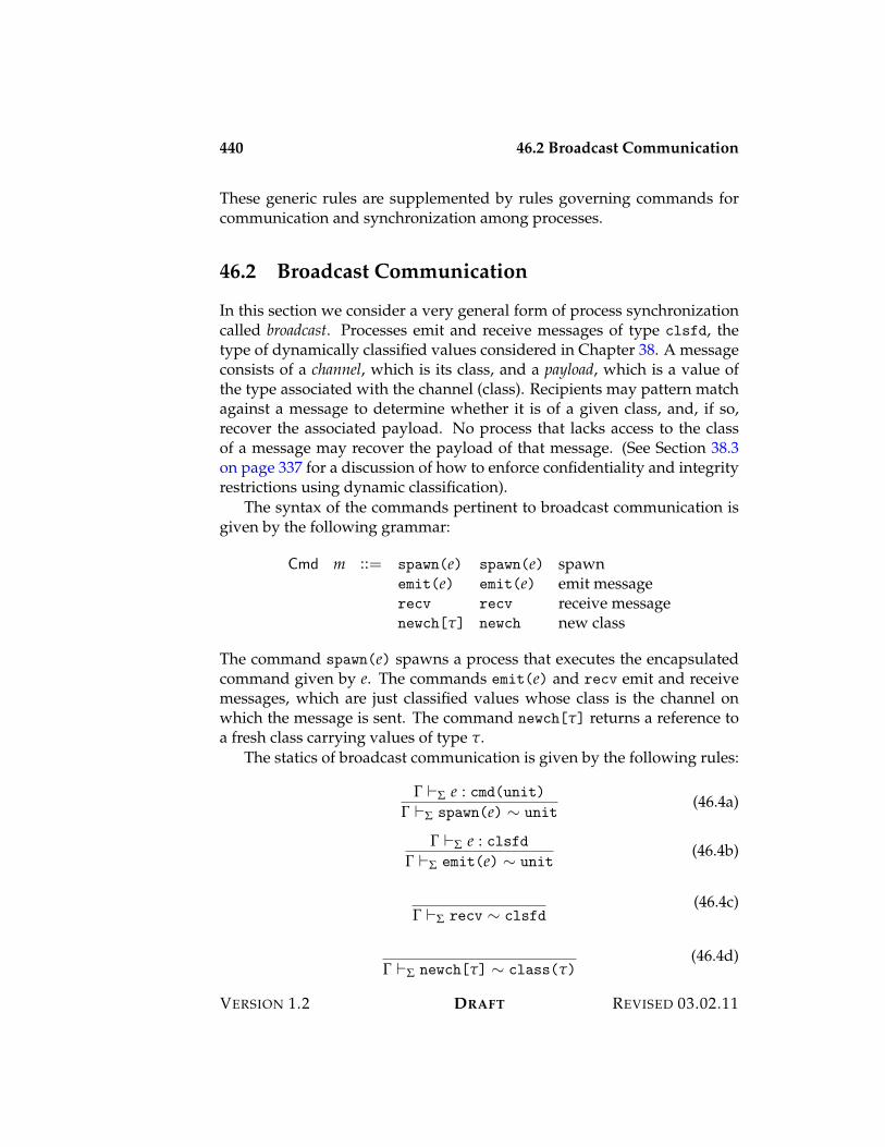
440 46.2 Broadcast Communication
These generic rules are supplemented by rules governing commands forcommunication and synchronization among processes.
46.2 Broadcast Communication
In this section we consider a very general form of process synchronizationcalled broadcast. Processes emit and receive messages of type clsfd, thetype of dynamically classified values considered in Chapter 38. A messageconsists of a channel, which is its class, and a payload, which is a value ofthe type associated with the channel (class). Recipients may pattern matchagainst a message to determine whether it is of a given class, and, if so,recover the associated payload. No process that lacks access to the classof a message may recover the payload of that message. (See Section 38.3on page 337 for a discussion of how to enforce confidentiality and integrityrestrictions using dynamic classification).
The syntax of the commands pertinent to broadcast communication isgiven by the following grammar:
Cmd m ::= spawn(e) spawn(e) spawnemit(e) emit(e) emit messagerecv recv receive messagenewch["] newch new class
The command spawn(e) spawns a process that executes the encapsulatedcommand given by e. The commands emit(e) and recv emit and receivemessages, which are just classified values whose class is the channel onwhich the message is sent. The command newch["] returns a reference toa fresh class carrying values of type ".
The statics of broadcast communication is given by the following rules:
! )$ e : cmd(unit)! )$ spawn(e) I unit
(46.4a)
! )$ e : clsfd! )$ emit(e) I unit
(46.4b)
! )$ recv I clsfd(46.4c)
! )$ newch["] I class(")(46.4d)
VERSION 1.2 DRAFT REVISED 03.02.11
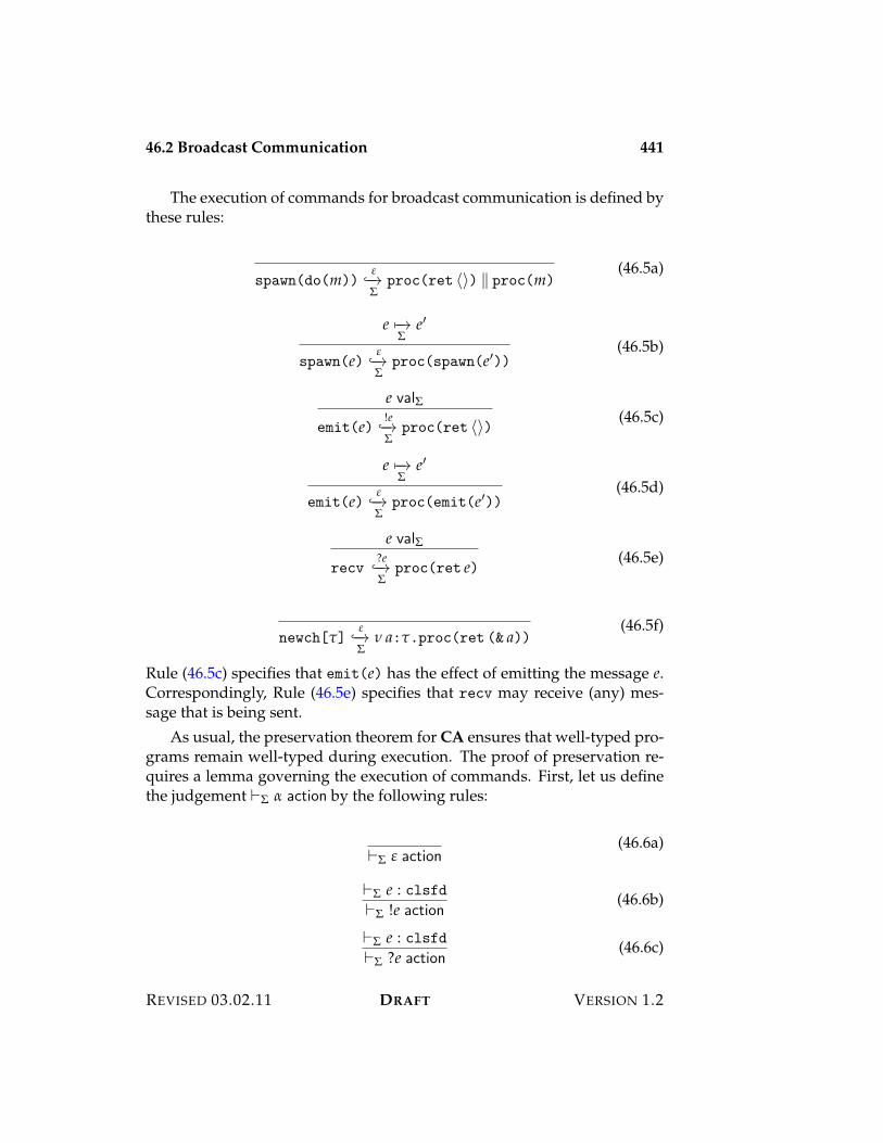
46.2 Broadcast Communication 441
The execution of commands for broadcast communication is defined bythese rules:
spawn(do(m))1
%$3$
proc(ret ?@) / proc(m)(46.5a)
e 5$3$
e%
spawn(e)1
%$3$
proc(spawn(e%))(46.5b)
e val$
emit(e)!e%$3
$proc(ret ?@) (46.5c)
e 5$3$
e%
emit(e)1
%$3$
proc(emit(e%))(46.5d)
e val$
recv?e%$3
$proc(ret e) (46.5e)
newch["]1
%$3$
0 a:".proc(ret (& a))(46.5f)
Rule (46.5c) specifies that emit(e) has the effect of emitting the message e.Correspondingly, Rule (46.5e) specifies that recv may receive (any) mes-sage that is being sent.
As usual, the preservation theorem for CA ensures that well-typed pro-grams remain well-typed during execution. The proof of preservation re-quires a lemma governing the execution of commands. First, let us definethe judgement )$ $ action by the following rules:
)$ 1 action(46.6a)
)$ e : clsfd)$ !e action
(46.6b)
)$ e : clsfd)$ ?e action
(46.6c)
REVISED 03.02.11 DRAFT VERSION 1.2
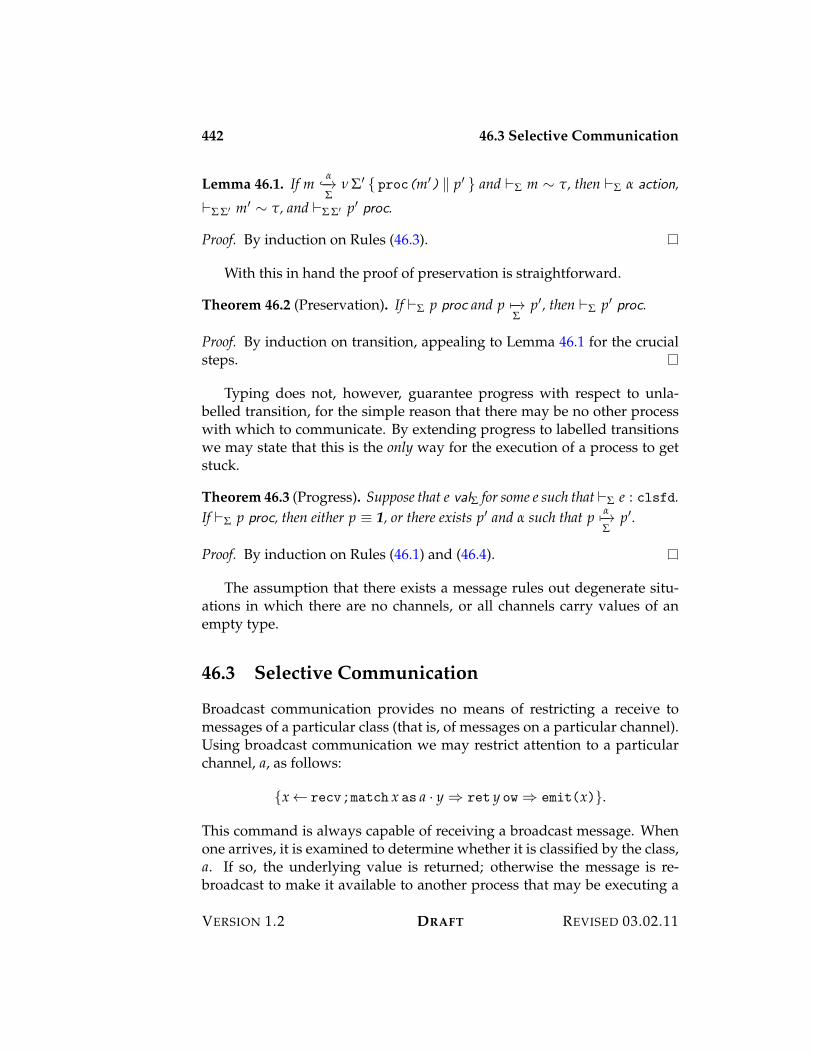
442 46.3 Selective Communication
Lemma 46.1. If m$%$3
$0 $% { proc(m%) / p% } and )$ m I ", then )$ $ action,
)$ $% m% I ", and )$ $% p% proc.
Proof. By induction on Rules (46.3).
With this in hand the proof of preservation is straightforward.
Theorem 46.2 (Preservation). If )$ p proc and p 5$3$
p%, then )$ p% proc.
Proof. By induction on transition, appealing to Lemma 46.1 for the crucialsteps.
Typing does not, however, guarantee progress with respect to unla-belled transition, for the simple reason that there may be no other processwith which to communicate. By extending progress to labelled transitionswe may state that this is the only way for the execution of a process to getstuck.
Theorem 46.3 (Progress). Suppose that e val$ for some e such that )$ e : clsfd.If )$ p proc, then either p 9 1, or there exists p% and $ such that p $5$3
$p%.
Proof. By induction on Rules (46.1) and (46.4).
The assumption that there exists a message rules out degenerate situ-ations in which there are no channels, or all channels carry values of anempty type.
46.3 Selective Communication
Broadcast communication provides no means of restricting a receive tomessages of a particular class (that is, of messages on a particular channel).Using broadcast communication we may restrict attention to a particularchannel, a, as follows:
{x 2 recv ; match x as a · y ; ret y ow ; emit(x)}.
This command is always capable of receiving a broadcast message. Whenone arrives, it is examined to determine whether it is classified by the class,a. If so, the underlying value is returned; otherwise the message is re-broadcast to make it available to another process that may be executing a
VERSION 1.2 DRAFT REVISED 03.02.11
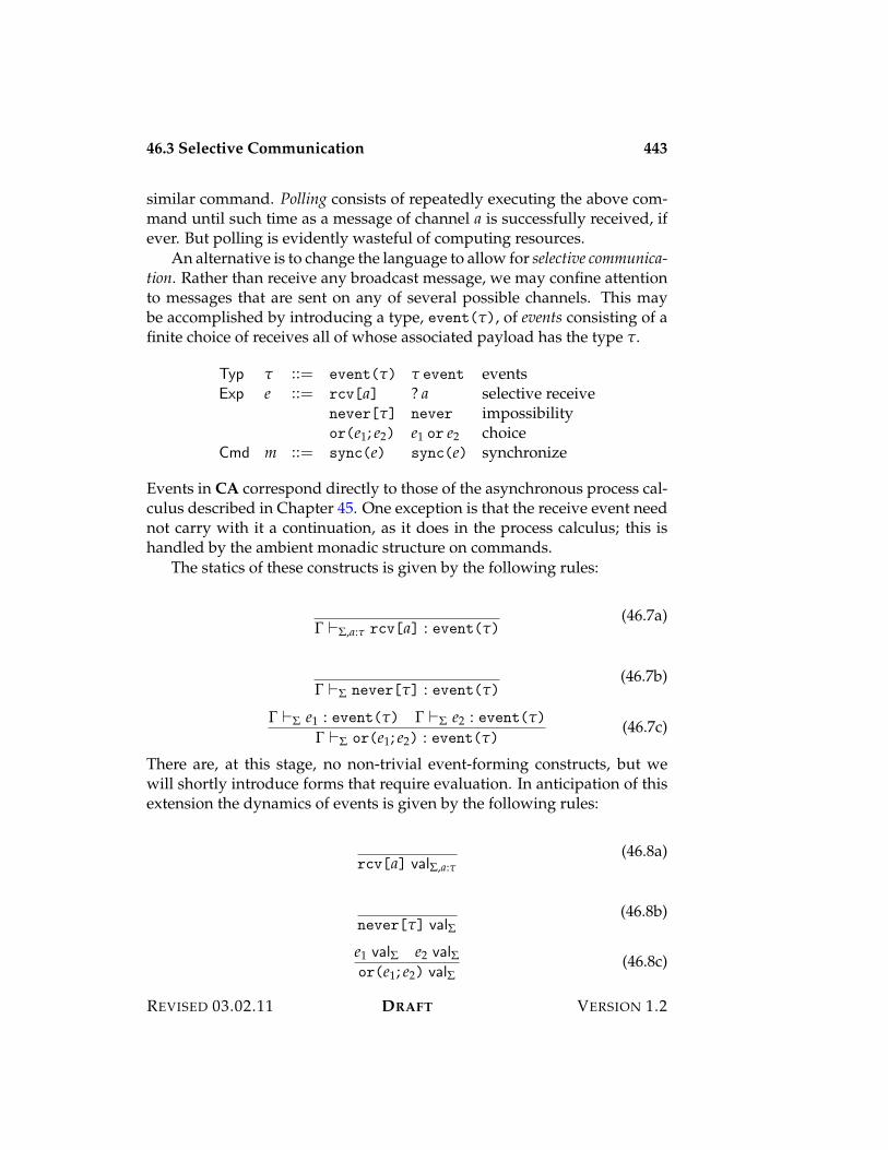
46.3 Selective Communication 443
similar command. Polling consists of repeatedly executing the above com-mand until such time as a message of channel a is successfully received, ifever. But polling is evidently wasteful of computing resources.
An alternative is to change the language to allow for selective communica-tion. Rather than receive any broadcast message, we may confine attentionto messages that are sent on any of several possible channels. This maybe accomplished by introducing a type, event("), of events consisting of afinite choice of receives all of whose associated payload has the type ".
Typ " ::= event(") " event eventsExp e ::= rcv[a] ? a selective receive
never["] never impossibilityor(e1; e2) e1 or e2 choice
Cmd m ::= sync(e) sync(e) synchronize
Events in CA correspond directly to those of the asynchronous process cal-culus described in Chapter 45. One exception is that the receive event neednot carry with it a continuation, as it does in the process calculus; this ishandled by the ambient monadic structure on commands.
The statics of these constructs is given by the following rules:
! )$,a:" rcv[a] : event(")(46.7a)
! )$ never["] : event(")(46.7b)
! )$ e1 : event(") ! )$ e2 : event(")! )$ or(e1; e2) : event(")
(46.7c)
There are, at this stage, no non-trivial event-forming constructs, but wewill shortly introduce forms that require evaluation. In anticipation of thisextension the dynamics of events is given by the following rules:
rcv[a] val$,a:"(46.8a)
never["] val$(46.8b)
e1 val$ e2 val$or(e1; e2) val$
(46.8c)
REVISED 03.02.11 DRAFT VERSION 1.2
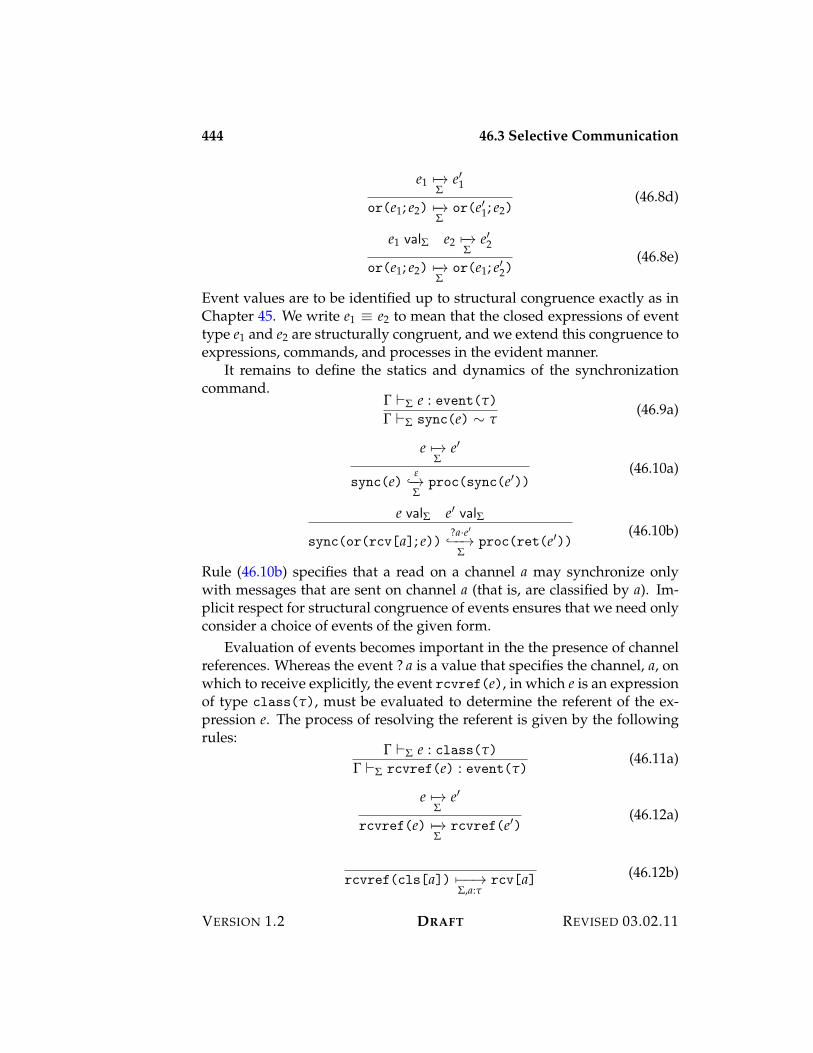
444 46.3 Selective Communication
e1 5$3$
e%1
or(e1; e2) 5$3$
or(e%1; e2)(46.8d)
e1 val$ e2 5$3$
e%2
or(e1; e2) 5$3$
or(e1; e%2)(46.8e)
Event values are to be identified up to structural congruence exactly as inChapter 45. We write e1 9 e2 to mean that the closed expressions of eventtype e1 and e2 are structurally congruent, and we extend this congruence toexpressions, commands, and processes in the evident manner.
It remains to define the statics and dynamics of the synchronizationcommand.
! )$ e : event(")! )$ sync(e) I "
(46.9a)
e 5$3$
e%
sync(e)1
%$3$
proc(sync(e%))(46.10a)
e val$ e% val$
sync(or(rcv[a]; e))?a·e%%$$3
$proc(ret(e%))
(46.10b)
Rule (46.10b) specifies that a read on a channel a may synchronize onlywith messages that are sent on channel a (that is, are classified by a). Im-plicit respect for structural congruence of events ensures that we need onlyconsider a choice of events of the given form.
Evaluation of events becomes important in the the presence of channelreferences. Whereas the event ? a is a value that specifies the channel, a, onwhich to receive explicitly, the event rcvref(e), in which e is an expressionof type class("), must be evaluated to determine the referent of the ex-pression e. The process of resolving the referent is given by the followingrules:
! )$ e : class(")! )$ rcvref(e) : event(")
(46.11a)
e 5$3$
e%
rcvref(e) 5$3$
rcvref(e%)(46.12a)
rcvref(cls[a]) 5$$3$,a:"
rcv[a] (46.12b)
VERSION 1.2 DRAFT REVISED 03.02.11
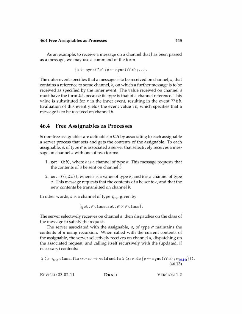
46.4 Free Assignables as Processes 445
As an example, to receive a message on a channel that has been passedas a message, we may use a command of the form
{x 2 sync(? a) ; y 2 sync(?? x) ; . . .}.
The outer event specifies that a message is to be received on channel, a, thatcontains a reference to some channel, b, on which a further message is to bereceived as specified by the inner event. The value received on channel amust have the form & b, because its type is that of a channel reference. Thisvalue is substituted for x in the inner event, resulting in the event ?? & b.Evaluation of this event yields the event value ? b, which specifies that amessage is to be received on channel b.
46.4 Free Assignables as Processes
Scope-free assignables are definable in CA by associating to each assignablea server process that sets and gets the contents of the assignable. To eachassignable, a, of type & is associated a server that selectively receives a mes-sage on channel a with one of two forms:
1. get · (& b), where b is a channel of type &. This message requests thatthe contents of a be sent on channel b.
2. set · (?e, & b@), where e is a value of type &, and b is a channel of type&. This message requests that the contents of a be set to e, and that thenew contents be transmitted on channel b.
In other words, a is a channel of type "srvr given by
[get : & class, set : & < & class].
The server selectively receives on channel a, then dispatches on the class ofthe message to satisfy the request.
The server associated with the assignable, a, of type & maintains thecontents of a using recursion. When called with the current contents ofthe assignable, the server selectively receives on channel a, dispatching onthe associated request, and calling itself recursively with the (updated, ifnecessary) contents:
! (u:"srvr class. fix srvr:& 3 void cmd is! (x:&. do {y 2 sync(?? u) ; e(46.14)})).(46.13)
REVISED 03.02.11 DRAFT VERSION 1.2
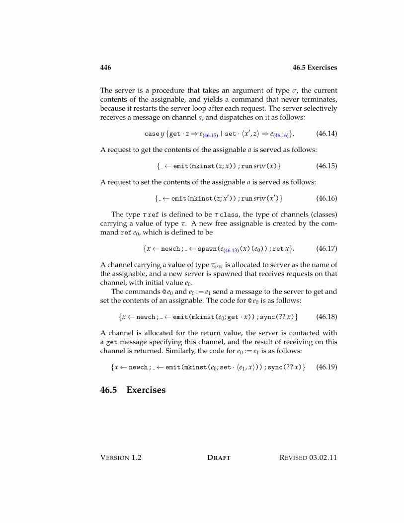
446 46.5 Exercises
The server is a procedure that takes an argument of type &, the currentcontents of the assignable, and yields a command that never terminates,because it restarts the server loop after each request. The server selectivelyreceives a message on channel a, and dispatches on it as follows:
case y {get · z ; e(46.15) | set · ?x%, z@ ; e(46.16)}. (46.14)
A request to get the contents of the assignable a is served as follows:
{ 2 emit(mkinst(z; x)) ; run srvr(x)} (46.15)
A request to set the contents of the assignable a is served as follows:
{ 2 emit(mkinst(z; x%)) ; run srvr(x%)} (46.16)
The type " ref is defined to be " class, the type of channels (classes)carrying a value of type ". A new free assignable is created by the com-mand ref e0, which is defined to be
{x 2 newch ; 2 spawn(e(46.13)(x)(e0)) ; ret x}. (46.17)
A channel carrying a value of type "srvr is allocated to server as the name ofthe assignable, and a new server is spawned that receives requests on thatchannel, with initial value e0.
The commands @ e0 and e0 := e1 send a message to the server to get andset the contents of an assignable. The code for @ e0 is as follows:
{x 2 newch ; 2 emit(mkinst(e0; get · x)) ; sync(?? x)} (46.18)
A channel is allocated for the return value, the server is contacted witha get message specifying this channel, and the result of receiving on thischannel is returned. Similarly, the code for e0 := e1 is as follows:
{x 2 newch ; 2 emit(mkinst(e0; set · ?e1, x@)) ; sync(?? x)} (46.19)
46.5 Exercises
VERSION 1.2 DRAFT REVISED 03.02.11
Chapter 47
Distributed Algol
A distributed computation is one that takes place at many different sites,each of which controls some resources located at that site. For example, thesites might be nodes on a network, and a resource might be a device or sen-sor located at that site, or a database controlled by that site. Only programsthat execute at a particular site may access the resources situated at thatsite. Consequently, command execution always takes place at a particularsite, called the locus of execution. Access to resources at a remote site froma local site is achieved by moving the locus of execution to the remote site,running code to access the local resource, and returning a value to the localsite.
In this chapter we consider an extension of Concurrent Algol, calledDistributed Algol, or DA, with a spatial type system that mediates access tolocated resources on a network. The type safety theorem ensures that allaccesses to a resource controlled by a site are through a program executingat that site, even though references to local resources may be freely passedaround to other sites on the network. The key idea is that channels andevents are located at a particular site, and that synchronization on an eventmay only occur at the site appropriate to that event. Issues of concurrency,which are to do with non-deterministic composition, are thereby cleanlyseparated from those of distribution, which are to do with the locality ofresources on a network.
47.1 Statics
The statics of DA is loosely inspired by the possible worlds interpretation ofmodal logic. Under that interpretation the truth of a proposition is relative
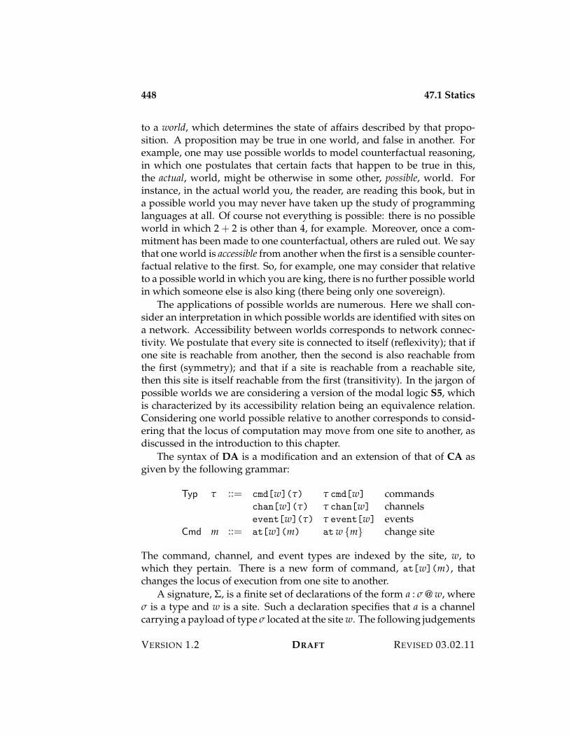
448 47.1 Statics
to a world, which determines the state of affairs described by that propo-sition. A proposition may be true in one world, and false in another. Forexample, one may use possible worlds to model counterfactual reasoning,in which one postulates that certain facts that happen to be true in this,the actual, world, might be otherwise in some other, possible, world. Forinstance, in the actual world you, the reader, are reading this book, but ina possible world you may never have taken up the study of programminglanguages at all. Of course not everything is possible: there is no possibleworld in which 2 + 2 is other than 4, for example. Moreover, once a com-mitment has been made to one counterfactual, others are ruled out. We saythat one world is accessible from another when the first is a sensible counter-factual relative to the first. So, for example, one may consider that relativeto a possible world in which you are king, there is no further possible worldin which someone else is also king (there being only one sovereign).
The applications of possible worlds are numerous. Here we shall con-sider an interpretation in which possible worlds are identified with sites ona network. Accessibility between worlds corresponds to network connec-tivity. We postulate that every site is connected to itself (reflexivity); that ifone site is reachable from another, then the second is also reachable fromthe first (symmetry); and that if a site is reachable from a reachable site,then this site is itself reachable from the first (transitivity). In the jargon ofpossible worlds we are considering a version of the modal logic S5, whichis characterized by its accessibility relation being an equivalence relation.Considering one world possible relative to another corresponds to consid-ering that the locus of computation may move from one site to another, asdiscussed in the introduction to this chapter.
The syntax of DA is a modification and an extension of that of CA asgiven by the following grammar:
Typ " ::= cmd[w](") " cmd[w] commandschan[w](") " chan[w] channelsevent[w](") " event[w] events
Cmd m ::= at[w](m) atw {m} change site
The command, channel, and event types are indexed by the site, w, towhich they pertain. There is a new form of command, at[w](m), thatchanges the locus of execution from one site to another.
A signature, $, is a finite set of declarations of the form a : & @ w, where& is a type and w is a site. Such a declaration specifies that a is a channelcarrying a payload of type & located at the site w. The following judgements
VERSION 1.2 DRAFT REVISED 03.02.11
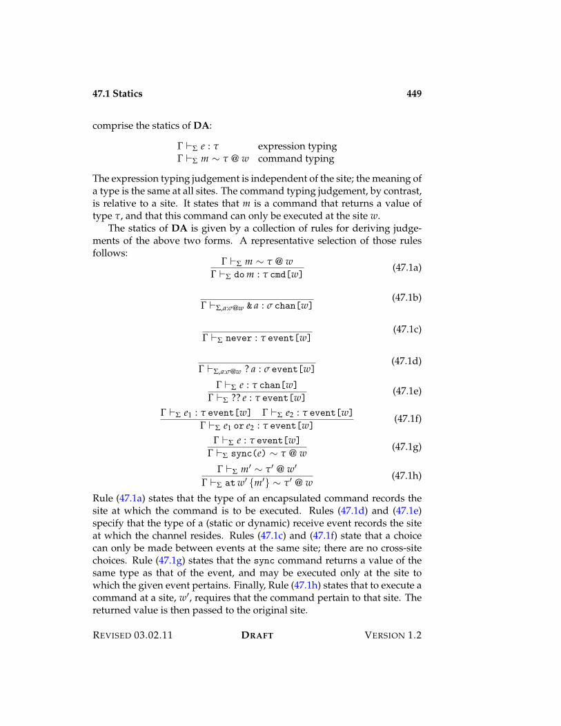
47.1 Statics 449
comprise the statics of DA:
! )$ e : " expression typing! )$ m I " @ w command typing
The expression typing judgement is independent of the site; the meaning ofa type is the same at all sites. The command typing judgement, by contrast,is relative to a site. It states that m is a command that returns a value oftype ", and that this command can only be executed at the site w.
The statics of DA is given by a collection of rules for deriving judge-ments of the above two forms. A representative selection of those rulesfollows:
! )$ m I " @ w! )$ dom : " cmd[w]
(47.1a)
! )$,a:&@w & a : & chan[w](47.1b)
! )$ never : " event[w](47.1c)
! )$,a:&@w ? a : & event[w](47.1d)
! )$ e : " chan[w]
! )$ ?? e : " event[w](47.1e)
! )$ e1 : " event[w] ! )$ e2 : " event[w]
! )$ e1 or e2 : " event[w](47.1f)
! )$ e : " event[w]
! )$ sync(e) I " @ w (47.1g)
! )$ m% I "% @ w%
! )$ atw% {m%} I "% @ w(47.1h)
Rule (47.1a) states that the type of an encapsulated command records thesite at which the command is to be executed. Rules (47.1d) and (47.1e)specify that the type of a (static or dynamic) receive event records the siteat which the channel resides. Rules (47.1c) and (47.1f) state that a choicecan only be made between events at the same site; there are no cross-sitechoices. Rule (47.1g) states that the sync command returns a value of thesame type as that of the event, and may be executed only at the site towhich the given event pertains. Finally, Rule (47.1h) states that to execute acommand at a site, w%, requires that the command pertain to that site. Thereturned value is then passed to the original site.
REVISED 03.02.11 DRAFT VERSION 1.2
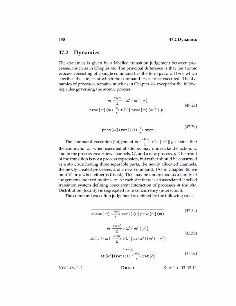
450 47.2 Dynamics
47.2 Dynamics
The dynamics is given by a labelled transition judgement between pro-cesses, much as in Chapter 46. The principal difference is that the atomicprocess consisting of a single command has the form proc[w](m), whichspecifies the site, w, at which the command, m, is to be executed. The dy-namics of processes remains much as in Chapter 46, except for the follow-ing rules governing the atomic process:
m$ @ w%$$3
$0 $% {m% / p }
proc[w](m)$5$3$
0 $% { proc[w](m%) / p }(47.2a)
proc[w](ret(?@)) 15$3$
stop(47.2b)
The command execution judgement m$ @ w%$$3
$0 $% {m% / p } states that
the command, m, when executed at site, w, may undertake the action, $,and in the process create new channels, $%, and a new process, p. The resultof the transition is not a process expression, but rather should be construedas a structure having three separable parts, the newly allocated channels,the newly created processes, and a new command. (As in Chapter 46, weomit $% or p when either is trivial.) This may be understood as a family ofjudgements indexed by sites, w. At each site there is an associated labelledtransition system defining concurrent interaction of processes at that site.Distribution (locality) is segregated from concurrency (interaction).
The command execution judgement is defined by the following rules:
spawn(m)1 @ w%$$3
$ret(?@) / proc[w](m)
(47.3a)
m$ @ w%%$$$3
$0 $% {m% / p% }
at[w%](m)$ @ w%$$3
$0 $% { at[w%](m%) / p% }
(47.3b)
e val$at[w%](ret(e))
1 @ w%$$3
$ret(e) (47.3c)
VERSION 1.2 DRAFT REVISED 03.02.11
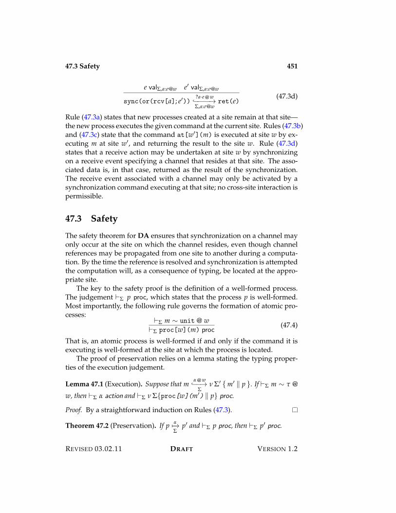
47.3 Safety 451
e val$,a:&@w e% val$,a:&@w
sync(or(rcv[a]; e%))?a·e @ w%$$$$3$,a:&@w
ret(e)(47.3d)
Rule (47.3a) states that new processes created at a site remain at that site—the new process executes the given command at the current site. Rules (47.3b)and (47.3c) state that the command at[w%](m) is executed at site w by ex-ecuting m at site w%, and returning the result to the site w. Rule (47.3d)states that a receive action may be undertaken at site w by synchronizingon a receive event specifying a channel that resides at that site. The asso-ciated data is, in that case, returned as the result of the synchronization.The receive event associated with a channel may only be activated by asynchronization command executing at that site; no cross-site interaction ispermissible.
47.3 Safety
The safety theorem for DA ensures that synchronization on a channel mayonly occur at the site on which the channel resides, even though channelreferences may be propagated from one site to another during a computa-tion. By the time the reference is resolved and synchronization is attemptedthe computation will, as a consequence of typing, be located at the appro-priate site.
The key to the safety proof is the definition of a well-formed process.The judgement )$ p proc, which states that the process p is well-formed.Most importantly, the following rule governs the formation of atomic pro-cesses:
)$ m I unit @ w)$ proc[w](m) proc
(47.4)
That is, an atomic process is well-formed if and only if the command it isexecuting is well-formed at the site at which the process is located.
The proof of preservation relies on a lemma stating the typing proper-ties of the execution judgement.
Lemma 47.1 (Execution). Suppose that m$ @ w%$$3
$0 $% {m% / p }. If )$ m I " @
w, then )$ $ action and )$ 0 ${proc[w](m%) / p} proc.
Proof. By a straightforward induction on Rules (47.3).
Theorem 47.2 (Preservation). If p $5$3$
p% and )$ p proc, then )$ p% proc.
REVISED 03.02.11 DRAFT VERSION 1.2
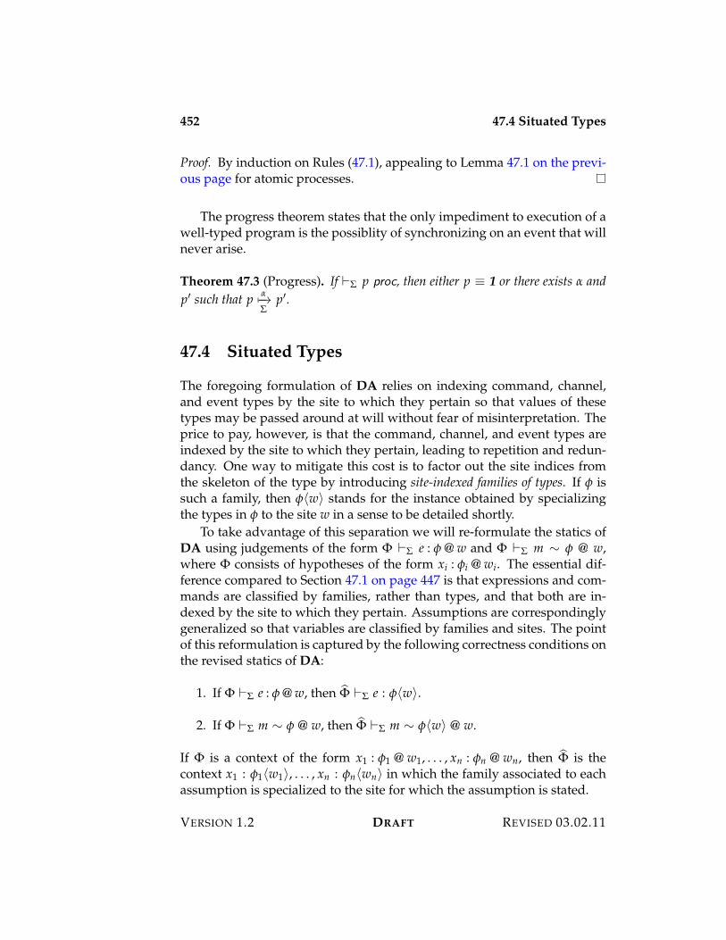
452 47.4 Situated Types
Proof. By induction on Rules (47.1), appealing to Lemma 47.1 on the previ-ous page for atomic processes.
The progress theorem states that the only impediment to execution of awell-typed program is the possiblity of synchronizing on an event that willnever arise.
Theorem 47.3 (Progress). If )$ p proc, then either p 9 1 or there exists $ andp% such that p $5$3
$p%.
47.4 Situated Types
The foregoing formulation of DA relies on indexing command, channel,and event types by the site to which they pertain so that values of thesetypes may be passed around at will without fear of misinterpretation. Theprice to pay, however, is that the command, channel, and event types areindexed by the site to which they pertain, leading to repetition and redun-dancy. One way to mitigate this cost is to factor out the site indices fromthe skeleton of the type by introducing site-indexed families of types. If ' issuch a family, then '?w@ stands for the instance obtained by specializingthe types in ' to the site w in a sense to be detailed shortly.
To take advantage of this separation we will re-formulate the statics ofDA using judgements of the form + )$ e : ' @ w and + )$ m I ' @ w,where + consists of hypotheses of the form xi : 'i @ wi. The essential dif-ference compared to Section 47.1 on page 447 is that expressions and com-mands are classified by families, rather than types, and that both are in-dexed by the site to which they pertain. Assumptions are correspondinglygeneralized so that variables are classified by families and sites. The pointof this reformulation is captured by the following correctness conditions onthe revised statics of DA:
1. If + )$ e : ' @ w, then )+ )$ e : '?w@.
2. If + )$ m I ' @ w, then )+ )$ m I '?w@ @ w.
If + is a context of the form x1 : '1 @ w1, . . . , xn : 'n @ wn, then )+ is thecontext x1 : '1?w1@, . . . , xn : 'n?wn@ in which the family associated to eachassumption is specialized to the site for which the assumption is stated.
VERSION 1.2 DRAFT REVISED 03.02.11
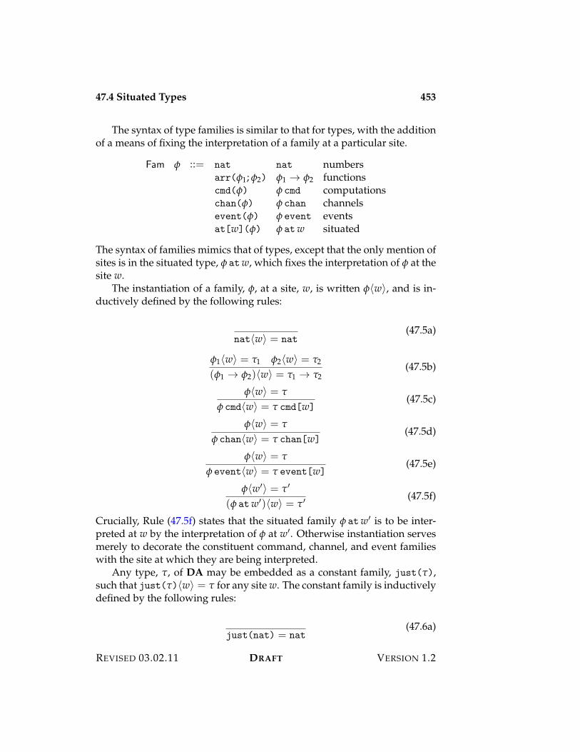
47.4 Situated Types 453
The syntax of type families is similar to that for types, with the additionof a means of fixing the interpretation of a family at a particular site.
Fam ' ::= nat nat numbersarr('1; '2) '1 3 '2 functionscmd(') ' cmd computationschan(') ' chan channelsevent(') ' event eventsat[w](') ' atw situated
The syntax of families mimics that of types, except that the only mention ofsites is in the situated type, ' atw, which fixes the interpretation of ' at thesite w.
The instantiation of a family, ', at a site, w, is written '?w@, and is in-ductively defined by the following rules:
nat?w@ = nat(47.5a)
'1?w@ = "1 '2?w@ = "2
('1 3 '2)?w@ = "1 3 "2(47.5b)
'?w@ = "
' cmd?w@ = " cmd[w](47.5c)
'?w@ = "
' chan?w@ = " chan[w](47.5d)
'?w@ = "
' event?w@ = " event[w](47.5e)
'?w%@ = "%
(' atw%)?w@ = "% (47.5f)
Crucially, Rule (47.5f) states that the situated family ' atw% is to be inter-preted at w by the interpretation of ' at w%. Otherwise instantiation servesmerely to decorate the constituent command, channel, and event familieswith the site at which they are being interpreted.
Any type, ", of DA may be embedded as a constant family, just("),such that just(")?w@ = " for any site w. The constant family is inductivelydefined by the following rules:
just(nat) = nat(47.6a)
REVISED 03.02.11 DRAFT VERSION 1.2
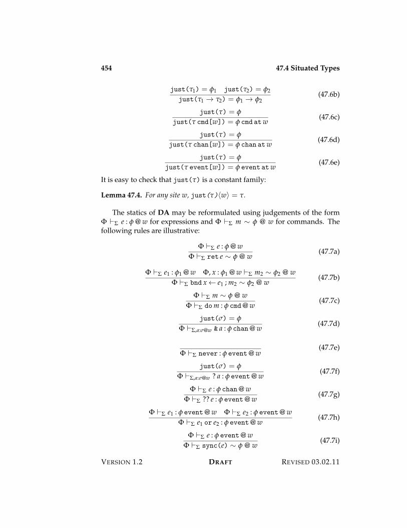
454 47.4 Situated Types
just("1) = '1 just("2) = '2
just("1 3 "2) = '1 3 '2(47.6b)
just(") = '
just(" cmd[w]) = ' cmd atw (47.6c)
just(") = '
just(" chan[w]) = ' chan atw (47.6d)
just(") = '
just(" event[w]) = ' event atw (47.6e)
It is easy to check that just(") is a constant family:
Lemma 47.4. For any site w, just(")?w@ = ".
The statics of DA may be reformulated using judgements of the form+ )$ e : ' @ w for expressions and + )$ m I ' @ w for commands. Thefollowing rules are illustrative:
+ )$ e : ' @ w+ )$ ret e I ' @ w
(47.7a)
+ )$ e1 : '1 @ w +, x : '1 @ w )$ m2 I '2 @ w+ )$ bnd x 2 e1 ; m2 I '2 @ w
(47.7b)
+ )$ m I ' @ w+ )$ dom : ' cmd @ w
(47.7c)
just(&) = '
+ )$,a:&@w & a : ' chan @ w(47.7d)
+ )$ never : ' event @ w(47.7e)
just(&) = '
+ )$,a:&@w ? a : ' event @ w(47.7f)
+ )$ e : ' chan @ w+ )$ ?? e : ' event @ w
(47.7g)
+ )$ e1 : ' event @ w + )$ e2 : ' event @ w+ )$ e1 or e2 : ' event @ w
(47.7h)
+ )$ e : ' event @ w+ )$ sync(e) I ' @ w
(47.7i)
VERSION 1.2 DRAFT REVISED 03.02.11
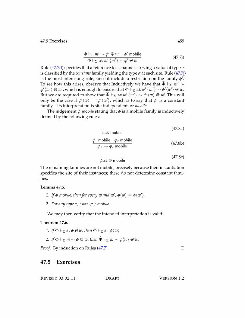
47.5 Exercises 455
+ )$ m% I '% @ w% '% mobile
+ )$ atw% {m%} I '% @ w(47.7j)
Rule (47.7d) specifies that a reference to a channel carrying a value of type &is classified by the constant family yielding the type & at each site. Rule (47.7j)is the most interesting rule, since it include a restriction on the family '%.To see how this arises, observe that Inductively we have that )+ )$ m% I'%?w%@ @ w%, which is enough to ensure that )+ )$ atw% {m%} I '%?w%@ @ w.But we are required to show that )+ )$ atw% {m%} I '%?w@ @ w! This willonly be the case if '%?w@ = '%?w%@, which is to say that '% is a constantfamily—its interpretation is site-independent, or mobile.
The judgement ' mobile stating that ' is a mobile family is inductivelydefined by the following rules:
nat mobile(47.8a)
'1 mobile '2 mobile
'1 3 '2 mobile(47.8b)
' atw mobile(47.8c)
The remaining families are not mobile, precisely because their instantiationspecifies the site of their instances; these do not determine constant fami-lies.
Lemma 47.5.
1. If ' mobile, then for every w and w%, '?w@ = '?w%@.
2. For any type ", just(") mobile.
We may then verify that the intended interpretation is valid:
Theorem 47.6.
1. If + )$ e : ' @ w, then )+ )$ e : '?w@.
2. If + )$ m I ' @ w, then )+ )$ m I '?w@ @ w.
Proof. By induction on Rules (47.7).
47.5 Exercises
REVISED 03.02.11 DRAFT VERSION 1.2

456 47.5 Exercises
VERSION 1.2 DRAFT REVISED 03.02.11

Part XVIII
Modularity

Chapter 48
Separate Compilation andLinking
48.1 Linking and Substitution
48.2 Exercises

460 48.2 Exercises
VERSION 1.2 DRAFT REVISED 03.02.11
Chapter 49
Basic Modules

462
VERSION 1.2 DRAFT REVISED 03.02.11
Chapter 50
Parameterized Modules

464
VERSION 1.2 DRAFT REVISED 03.02.11
Part XIX
Equivalence

Chapter 51
Equational Reasoning for T
The beauty of functional programming is that equality of expressions in afunctional language corresponds very closely to familiar patterns of math-ematical reasoning. For example, in the language L{nat3} of Chapter 12in which we can express addition as the function plus, the expressions
! (x:nat. ! (y:nat. plus(x)(y)))
and! (x:nat. ! (y:nat. plus(y)(x)))
are equal. In other words, the addition function as programmed in L{nat3}is commutative.
This may seem to be obviously true, but why, precisely, is it so? Moreimportantly, what do we even mean when we say that two expressions of aprogramming language are equal in this sense? It is intuitively obvious thatthese two expressions are not definitionally equivalent, because they cannotbe shown equivalent by symbolic execution. One may say that these twoexpressions are definitionally inequivalent because they describe differentalgorithms: one proceeds by recursion on x, the other by recursion on y.On the other hand, the two expressions are interchangeable in any com-plete computation of a natural number, because the only use we can makeof them is to apply them to arguments and compute the result. We saythat two functions are extensionally equivalent if they give equal results forequal arguments—in particular, they agree on all possible arguments. Sincetheir behavior on arguments is all that matters for calculating observableresults, we may expect that extensionally equivalent functions are equal inthe sense of being interchangeable in all complete programs. Thinking of
468 51.1 Observational Equivalence
the programs in which these functions occur as observations of their behav-ior, we say that the these functions are observationally equivalent. The mainresult of this chapter is that observational and extensional equivalence coin-cide for a variant of L{nat3} in which the successor is evaluated eagerly,so that a value of type nat is a numeral.
51.1 Observational Equivalence
When are two expressions equal? Whenever we cannot tell them apart!This may seem tautological, but it is not, because it depends on what weconsider to be a means of telling expressions apart. What “experiment”are we permitted to perform on expressions in order to distinguish them?What counts as an observation that, if different for two expressions, is asure sign that they are different?
If we permit ourselves to consider the syntactic details of the expres-sions, then very few expressions could be considered equal. For example,if it is deemed significant that an expression contains, say, more than onefunction application, or that it has an occurrence of !-abstraction, then veryfew expressions would come out as equivalent. But such considerationsseem silly, because they conflict with the intuition that the significance ofan expression lies in its contribution to the outcome of a computation, andnot to the process of obtaining that outcome. In short, if two expressionsmake the same contribution to the outcome of a complete program, thenthey ought to be regarded as equal.
We must fix what we mean by a complete program. Two considerationsinform the definition. First, the dynamics of L{nat3} is given only forexpressions without free variables, so a complete program should clearlybe a closed expression. Second, the outcome of a computation should beobservable, so that it is evident whether the outcome of two computationsdiffers or not. We define a complete program to be a closed expression of typenat, and define the observable behavior of the program to be the numeral towhich it evaluates.
An experiment on, or observation about, an expression is any means ofusing that expression within a complete program. We define an expressioncontext to be an expression with a “hole” in it serving as a placeholder foranother expression. The hole is permitted to occur anywhere, includingwithin the scope of a binder. The bound variables within whose scope thehole lies are said to be exposed (to capture) by the expression context. Thesevariables may be assumed, without loss of generality, to be distinct from
VERSION 1.2 DRAFT REVISED 03.02.11
51.1 Observational Equivalence 469
one another. A program context is a closed expression context of type nat—that is, it is a complete program with a hole in it. The meta-variable Cstands for any expression context.
Replacement is the process of filling a hole in an expression context, C,with an expression, e, which is written C{e}. Importantly, the free vari-ables of e that are exposed by C are captured by replacement (which is whyreplacement is not a form of substitution, which is defined so as to avoidcapture). If C is a program context, then C{e} is a complete program iffall free variables of e are captured by the replacement. For example, ifC = ! (x:nat. 8), and e = x + x, then
C{e} = ! (x:nat. x + x).
The free occurrences of x in e are captured by the !-abstraction as a resultof the replacement of the hole in C by e.
We sometimes write C{8} to emphasize the occurrence of the hole inC. Expression contexts are closed under composition in that if C1 and C2 areexpression contexts, then so is
C{8} % C1{C2{8}},
and we have C{e} = C1{C2{e}}. The trivial, or identity, expression contextis the “bare hole”, written 8, for which 8{e} = e.
The statics of expressions of L{nat3} is extended to expression con-texts by defining the typing judgement
C : (! $ ") ! (!% $ "%)
so that if ! ) e : ", then !% ) C{e} : "%. This judgement may be inductivelydefined by a collection of rules derived from the statics of L{nat3} (seeRules (12.1)). Some representative rules are as follows:
8 : (! $ ") ! (! $ ") (51.1a)
C : (! $ ") ! (!% $ nat)
s(C) : (! $ ") ! (!% $ nat)(51.1b)
C : (! $ ") ! (!% $ nat) !% ) e0 : "% !%, x : nat, y : "% ) e1 : "%
natrec C {z; e0 | s(x) with y ; e1} : (! $ ") ! (!% $ "%)(51.1c)
!% ) e : nat C0 : (! $ ") ! (!% $ "%) !%, x : nat, y : "% ) e1 : "%
natrec e {z; C0 | s(x) with y ; e1} : (! $ ") ! (!% $ "%)(51.1d)
REVISED 03.02.11 DRAFT VERSION 1.2
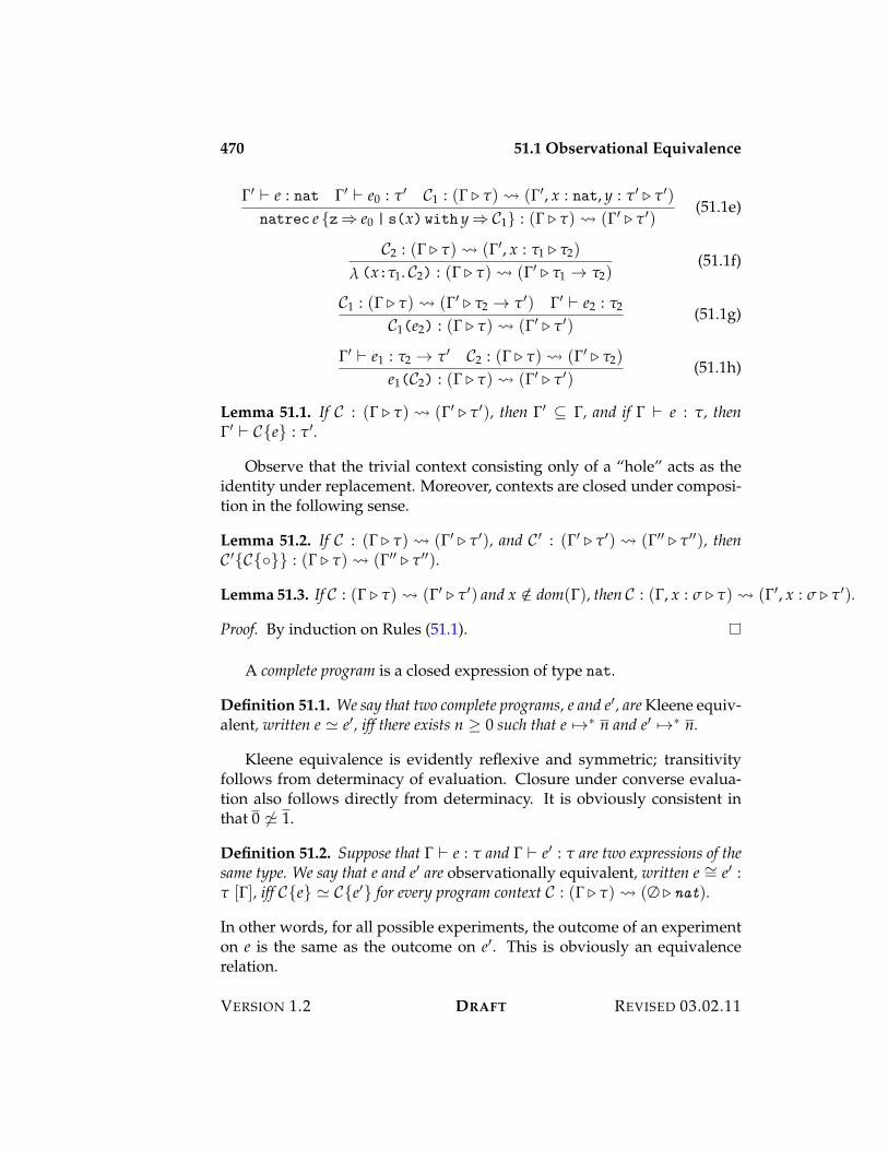
470 51.1 Observational Equivalence
!% ) e : nat !% ) e0 : "% C1 : (! $ ") ! (!%, x : nat, y : "% $ "%)
natrec e {z; e0 | s(x) with y ; C1} : (! $ ") ! (!% $ "%)(51.1e)
C2 : (! $ ") ! (!%, x : "1 $ "2)
! (x:"1. C2) : (! $ ") ! (!% $ "1 3 "2)(51.1f)
C1 : (! $ ") ! (!% $ "2 3 "%) !% ) e2 : "2
C1(e2) : (! $ ") ! (!% $ "%)(51.1g)
!% ) e1 : "2 3 "% C2 : (! $ ") ! (!% $ "2)
e1(C2) : (! $ ") ! (!% $ "%)(51.1h)
Lemma 51.1. If C : (! $ ") ! (!% $ "%), then !% - !, and if ! ) e : ", then!% ) C{e} : "%.
Observe that the trivial context consisting only of a “hole” acts as theidentity under replacement. Moreover, contexts are closed under composi-tion in the following sense.
Lemma 51.2. If C : (! $ ") ! (!% $ "%), and C % : (!% $ "%) ! (!%% $ "%%), thenC %{C{8}} : (! $ ") ! (!%% $ "%%).
Lemma 51.3. If C : (! $ ") ! (!% $ "%) and x /+ dom(!), then C : (!, x : & $ ") ! (!%, x : & $ "%).
Proof. By induction on Rules (51.1).
A complete program is a closed expression of type nat.
Definition 51.1. We say that two complete programs, e and e%, are Kleene equiv-alent, written e P e%, iff there exists n 7 0 such that e 531 n and e% 531 n.
Kleene equivalence is evidently reflexive and symmetric; transitivityfollows from determinacy of evaluation. Closure under converse evalua-tion also follows directly from determinacy. It is obviously consistent inthat 0 ,P 1.
Definition 51.2. Suppose that ! ) e : " and ! ) e% : " are two expressions of thesame type. We say that e and e% are observationally equivalent, written e I= e% :" [!], iff C{e} P C{e%} for every program context C : (! $ ") ! (# $ nat).
In other words, for all possible experiments, the outcome of an experimenton e is the same as the outcome on e%. This is obviously an equivalencerelation.
VERSION 1.2 DRAFT REVISED 03.02.11
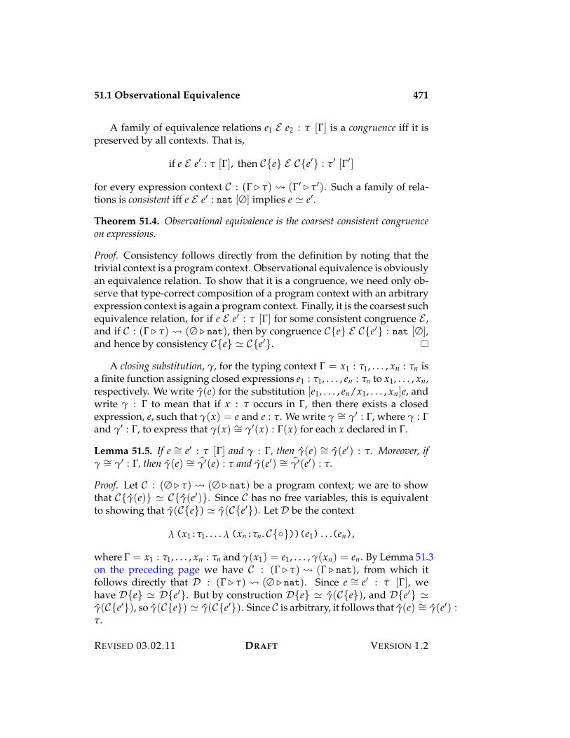
51.1 Observational Equivalence 471
A family of equivalence relations e1 E e2 : " [!] is a congruence iff it ispreserved by all contexts. That is,
if e E e% : " [!], then C{e} E C{e%} : "% [!%]
for every expression context C : (! $ ") ! (!% $ "%). Such a family of rela-tions is consistent iff e E e% : nat [#] implies e P e%.
Theorem 51.4. Observational equivalence is the coarsest consistent congruenceon expressions.
Proof. Consistency follows directly from the definition by noting that thetrivial context is a program context. Observational equivalence is obviouslyan equivalence relation. To show that it is a congruence, we need only ob-serve that type-correct composition of a program context with an arbitraryexpression context is again a program context. Finally, it is the coarsest suchequivalence relation, for if e E e% : " [!] for some consistent congruence E ,and if C : (! $ ") ! (# $ nat), then by congruence C{e} E C{e%} : nat [#],and hence by consistency C{e} P C{e%}.
A closing substitution, /, for the typing context ! = x1 : "1, . . . , xn : "n isa finite function assigning closed expressions e1 : "1, . . . , en : "n to x1, . . . , xn,respectively. We write /(e) for the substitution [e1, . . . , en/x1, . . . , xn]e, andwrite / : ! to mean that if x : " occurs in !, then there exists a closedexpression, e, such that /(x) = e and e : ". We write / I= /% : !, where / : !and /% : !, to express that /(x) I= /%(x) : !(x) for each x declared in !.
Lemma 51.5. If e I= e% : " [!] and / : !, then /(e) I= /(e%) : ". Moreover, if/ I= /% : !, then /(e) I= )/%(e) : " and /(e%) I= )/%(e%) : ".
Proof. Let C : (# $ ") ! (# $ nat) be a program context; we are to showthat C{/(e)} P C{/(e%)}. Since C has no free variables, this is equivalentto showing that /(C{e}) P /(C{e%}). Let D be the context
! (x1:"1. . . . ! (xn:"n. C{8}))(e1) . . .(en),
where ! = x1 : "1, . . . , xn : "n and /(x1) = e1, . . . , /(xn) = en. By Lemma 51.3on the preceding page we have C : (! $ ") ! (! $ nat), from which itfollows directly that D : (! $ ") ! (# $ nat). Since e I= e% : " [!], wehave D{e} P D{e%}. But by construction D{e} P /(C{e}), and D{e%} P/(C{e%}), so /(C{e}) P /(C{e%}). Since C is arbitrary, it follows that /(e) I= /(e%) :".
REVISED 03.02.11 DRAFT VERSION 1.2
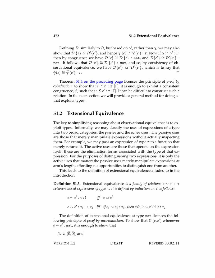
472 51.2 Extensional Equivalence
Defining D% similarly to D, but based on /%, rather than /, we may alsoshow that D%{e} P D%{e%}, and hence )/%(e) I= )/%(e%) : ". Now if / I= /% : !,then by congruence we have D{e} I= D%{e} : nat, and D{e%} I= D%{e%} :nat. It follows that D{e%} I= D%{e%} : nat, and so, by consistency of ob-servational equivalence, we have D{e%} P D%{e%}, which is to say that/(e) I= )/%(e%) : ".
Theorem 51.4 on the preceding page licenses the principle of proof bycoinduction: to show that e I= e% : " [!], it is enough to exhibit a consistentcongruence, E , such that e E e% : " [!]. It can be difficult to construct such arelation. In the next section we will provide a general method for doing sothat exploits types.
51.2 Extensional Equivalence
The key to simplifying reasoning about observational equivalence is to ex-ploit types. Informally, we may classify the uses of expressions of a typeinto two broad categories, the passive and the active uses. The passive usesare those that merely manipulate expressions without actually inspectingthem. For example, we may pass an expression of type " to a function thatmerely returns it. The active uses are those that operate on the expressionitself; these are the elimination forms associated with the type of that ex-pression. For the purposes of distinguishing two expressions, it is only theactive uses that matter; the passive uses merely manipulate expressions atarm’s length, affording no opportunities to distinguish one from another.
This leads to the definition of extensional equivalence alluded to in theintroduction.
Definition 51.3. Extensional equivalence is a family of relations e I e% : "between closed expressions of type ". It is defined by induction on " as follows:
e I e% : nat iff e P e%
e I e% : "1 3 "2 iff if e1 I e%1 : "1, then e(e1) I e%(e%1) : "2
The definition of extensional equivalence at type nat licenses the fol-lowing principle of proof by nat-induction. To show that E (e, e%) whenevere I e% : nat, it is enough to show that
1. E (0, 0), and
VERSION 1.2 DRAFT REVISED 03.02.11
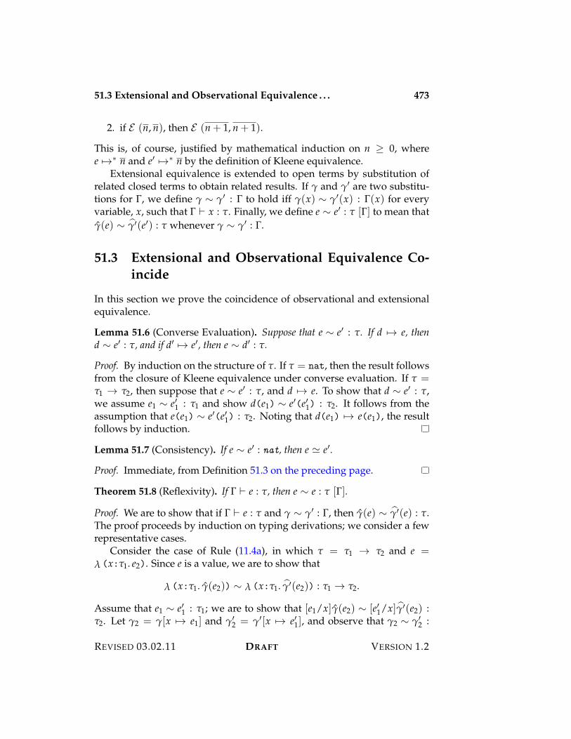
51.3 Extensional and Observational Equivalence . . . 473
2. if E (n, n), then E (n + 1, n + 1).
This is, of course, justified by mathematical induction on n 7 0, wheree 531 n and e% 531 n by the definition of Kleene equivalence.
Extensional equivalence is extended to open terms by substitution ofrelated closed terms to obtain related results. If / and /% are two substitu-tions for !, we define / I /% : ! to hold iff /(x) I /%(x) : !(x) for everyvariable, x, such that ! ) x : ". Finally, we define e I e% : " [!] to mean that/(e) I )/%(e%) : " whenever / I /% : !.
51.3 Extensional and Observational Equivalence Co-incide
In this section we prove the coincidence of observational and extensionalequivalence.
Lemma 51.6 (Converse Evaluation). Suppose that e I e% : ". If d 53 e, thend I e% : ", and if d% 53 e%, then e I d% : ".
Proof. By induction on the structure of ". If " = nat, then the result followsfrom the closure of Kleene equivalence under converse evaluation. If " ="1 3 "2, then suppose that e I e% : ", and d 53 e. To show that d I e% : ",we assume e1 I e%1 : "1 and show d(e1) I e%(e%1) : "2. It follows from theassumption that e(e1) I e%(e%1) : "2. Noting that d(e1) 53 e(e1), the resultfollows by induction.
Lemma 51.7 (Consistency). If e I e% : nat, then e P e%.
Proof. Immediate, from Definition 51.3 on the preceding page.
Theorem 51.8 (Reflexivity). If ! ) e : ", then e I e : " [!].
Proof. We are to show that if ! ) e : " and / I /% : !, then /(e) I )/%(e) : ".The proof proceeds by induction on typing derivations; we consider a fewrepresentative cases.
Consider the case of Rule (11.4a), in which " = "1 3 "2 and e =! (x:"1. e2). Since e is a value, we are to show that
! (x:"1. /(e2)) I ! (x:"1. )/%(e2)) : "1 3 "2.
Assume that e1 I e%1 : "1; we are to show that [e1/x]/(e2) I [e%1/x] )/%(e2) :"2. Let /2 = /[x 53 e1] and /%
2 = /%[x 53 e%1], and observe that /2 I /%2 :
REVISED 03.02.11 DRAFT VERSION 1.2
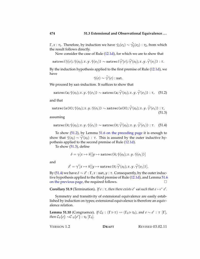
474 51.3 Extensional and Observational Equivalence . . .
!, x : "1. Therefore, by induction we have /2(e2) I /%2(e2) : "2, from which
the result follows directly.Now consider the case of Rule (12.1d), for which we are to show that
natrec(/(e); /(e0); x.y./(e1)) I natrec( )/%(e); )/%(e0); x.y. )/%(e1)) : ".
By the induction hypothesis applied to the first premise of Rule (12.1d), wehave
/(e) I )/%(e) : nat.
We proceed by nat-induction. It suffices to show that
natrec(z; /(e0); x.y./(e1)) I natrec(z; )/%(e0); x.y. )/%(e1)) : ", (51.2)
and that
natrec(s(n); /(e0); x.y./(e1)) I natrec(s(n); )/%(e0); x.y. )/%(e1)) : ",(51.3)
assuming
natrec(n; /(e0); x.y./(e1)) I natrec(n; )/%(e0); x.y. )/%(e1)) : ". (51.4)
To show (51.2), by Lemma 51.6 on the preceding page it is enough toshow that /(e0) I )/%(e0) : ". This is assured by the outer inductive hy-pothesis applied to the second premise of Rule (12.1d).
To show (51.3), define
2 = /[x 53 n][y 53 natrec(n; /(e0); x.y./(e1))]
and2% = /%[x 53 n][y 53 natrec(n; )/%(e0); x.y. )/%(e1))].
By (51.4) we have 2 I 2% : !, x : nat, y : ". Consequently, by the outer induc-tive hypothesis applied to the third premise of Rule (12.1d), and Lemma 51.6on the previous page, the required follows.
Corollary 51.9 (Termination). If e : ", then there exists e% val such that e 531 e%.
Symmetry and transitivity of extensional equivalence are easily estab-lished by induction on types; extensional equivalence is therefore an equiv-alence relation.
Lemma 51.10 (Congruence). If C0 : (! $ ") ! (!0 $ "0), and e I e% : " [!],then C0{e} IC 0{e%} : "0 [!0].
VERSION 1.2 DRAFT REVISED 03.02.11
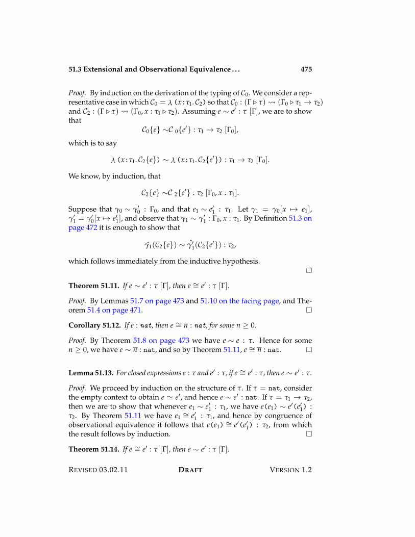
51.3 Extensional and Observational Equivalence . . . 475
Proof. By induction on the derivation of the typing of C0. We consider a rep-resentative case in which C0 = ! (x:"1. C2) so that C0 : (! $ ") ! (!0 $ "1 3 "2)and C2 : (! $ ") ! (!0, x : "1 $ "2). Assuming e I e% : " [!], we are to showthat
C0{e} IC 0{e%} : "1 3 "2 [!0],
which is to say
! (x:"1. C2{e}) I ! (x:"1. C2{e%}) : "1 3 "2 [!0].
We know, by induction, that
C2{e} IC 2{e%} : "2 [!0, x : "1].
Suppose that /0 I /%0 : !0, and that e1 I e%1 : "1. Let /1 = /0[x 53 e1],
/%1 = /%
0[x 53 e%1], and observe that /1 I /%1 : !0, x : "1. By Definition 51.3 on
page 472 it is enough to show that
/1(C2{e}) I /%1(C2{e%}) : "2,
which follows immediately from the inductive hypothesis.
Theorem 51.11. If e I e% : " [!], then e I= e% : " [!].
Proof. By Lemmas 51.7 on page 473 and 51.10 on the facing page, and The-orem 51.4 on page 471.
Corollary 51.12. If e : nat, then e I= n : nat, for some n 7 0.
Proof. By Theorem 51.8 on page 473 we have e I e : ". Hence for somen 7 0, we have e I n : nat, and so by Theorem 51.11, e I= n : nat.
Lemma 51.13. For closed expressions e : " and e% : ", if e I= e% : ", then e I e% : ".
Proof. We proceed by induction on the structure of ". If " = nat, considerthe empty context to obtain e P e%, and hence e I e% : nat. If " = "1 3 "2,then we are to show that whenever e1 I e%1 : "1, we have e(e1) I e%(e%1) :"2. By Theorem 51.11 we have e1 I= e%1 : "1, and hence by congruence ofobservational equivalence it follows that e(e1) I= e%(e%1) : "2, from whichthe result follows by induction.
Theorem 51.14. If e I= e% : " [!], then e I e% : " [!].
REVISED 03.02.11 DRAFT VERSION 1.2
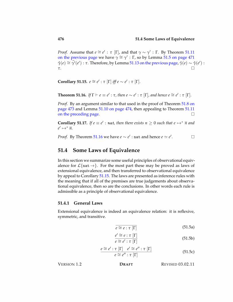
476 51.4 Some Laws of Equivalence
Proof. Assume that e I= e% : " [!], and that / I /% : !. By Theorem 51.11on the previous page we have / I= /% : !, so by Lemma 51.5 on page 471/(e) I= )/%(e%) : ". Therefore, by Lemma 51.13 on the previous page, /(e) I /(e%) :".
Corollary 51.15. e I= e% : " [!] iff e I e% : " [!].
Theorem 51.16. If ! ) e 9 e% : ", then e I e% : " [!], and hence e I= e% : " [!].
Proof. By an argument similar to that used in the proof of Theorem 51.8 onpage 473 and Lemma 51.10 on page 474, then appealing to Theorem 51.11on the preceding page.
Corollary 51.17. If e 9 e% : nat, then there exists n 7 0 such that e 531 n ande% 531 n.
Proof. By Theorem 51.16 we have e I e% : nat and hence e P e%.
51.4 Some Laws of Equivalence
In this section we summarize some useful principles of observational equiv-alence for L{nat3}. For the most part these may be proved as laws ofextensional equivalence, and then transferred to observational equivalenceby appeal to Corollary 51.15. The laws are presented as inference rules withthe meaning that if all of the premises are true judgements about observa-tional equivalence, then so are the conclusions. In other words each rule isadmissible as a principle of observational equivalence.
51.4.1 General Laws
Extensional equivalence is indeed an equivalence relation: it is reflexive,symmetric, and transitive.
e I= e : " [!] (51.5a)
e% I= e : " [!]e I= e% : " [!]
(51.5b)
e I= e% : " [!] e% I= e%% : " [!]e I= e%% : " [!]
(51.5c)
VERSION 1.2 DRAFT REVISED 03.02.11
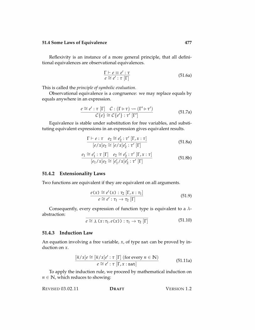
51.4 Some Laws of Equivalence 477
Reflexivity is an instance of a more general principle, that all defini-tional equivalences are observational equivalences.
! ) e 9 e% : "e I= e% : " [!] (51.6a)
This is called the principle of symbolic evaluation.Observational equivalence is a congruence: we may replace equals by
equals anywhere in an expression.
e I= e% : " [!] C : (! $ ") ! (!% $ "%)
C{e} I= C{e%} : "% [!%](51.7a)
Equivalence is stable under substitution for free variables, and substi-tuting equivalent expressions in an expression gives equivalent results.
! ) e : " e2 I= e%2 : "% [!, x : "]
[e/x]e2 I= [e/x]e%2 : "% [!](51.8a)
e1 I= e%1 : " [!] e2 I= e%2 : "% [!, x : "]
[e1/x]e2 I= [e%1/x]e%2 : "% [!](51.8b)
51.4.2 Extensionality Laws
Two functions are equivalent if they are equivalent on all arguments.
e(x) I= e%(x) : "2 [!, x : "1]
e I= e% : "1 3 "2 [!](51.9)
Consequently, every expression of function type is equivalent to a !-abstraction:
e I= ! (x:"1. e(x)) : "1 3 "2 [!] (51.10)
51.4.3 Induction Law
An equation involving a free variable, x, of type nat can be proved by in-duction on x.
[n/x]e I= [n/x]e% : " [!] (for every n + N)
e I= e% : " [!, x : nat](51.11a)
To apply the induction rule, we proceed by mathematical induction onn + N, which reduces to showing:
REVISED 03.02.11 DRAFT VERSION 1.2
478 51.5 Exercises
1. [z/x]e I= [z/x]e% : " [!], and
2. [s(n)/x]e I= [s(n)/x]e% : " [!], if [n/x]e I= [n/x]e% : " [!].
51.5 Exercises
VERSION 1.2 DRAFT REVISED 03.02.11
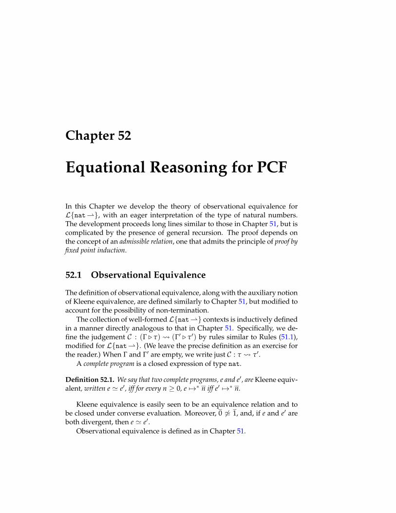
Chapter 52
Equational Reasoning for PCF
In this Chapter we develop the theory of observational equivalence forL{nat"}, with an eager interpretation of the type of natural numbers.The development proceeds long lines similar to those in Chapter 51, but iscomplicated by the presence of general recursion. The proof depends onthe concept of an admissible relation, one that admits the principle of proof byfixed point induction.
52.1 Observational Equivalence
The definition of observational equivalence, along with the auxiliary notionof Kleene equivalence, are defined similarly to Chapter 51, but modified toaccount for the possibility of non-termination.
The collection of well-formed L{nat"} contexts is inductively definedin a manner directly analogous to that in Chapter 51. Specifically, we de-fine the judgement C : (! $ ") ! (!% $ "%) by rules similar to Rules (51.1),modified for L{nat"}. (We leave the precise definition as an exercise forthe reader.) When ! and !% are empty, we write just C : " ! "%.
A complete program is a closed expression of type nat.
Definition 52.1. We say that two complete programs, e and e%, are Kleene equiv-alent, written e P e%, iff for every n 7 0, e 531 n iff e% 531 n.
Kleene equivalence is easily seen to be an equivalence relation and tobe closed under converse evaluation. Moreover, 0 ,P 1, and, if e and e% areboth divergent, then e P e%.
Observational equivalence is defined as in Chapter 51.
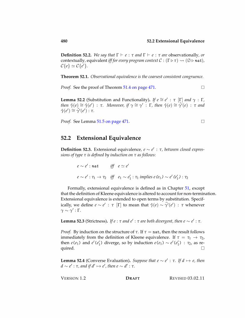
480 52.2 Extensional Equivalence
Definition 52.2. We say that ! ) e : " and ! ) e : " are observationally, orcontextually, equivalent iff for every program context C : (! $ ") ! (# $ nat),C{e} P C{e%}.
Theorem 52.1. Observational equivalence is the coarsest consistent congruence.
Proof. See the proof of Theorem 51.4 on page 471.
Lemma 52.2 (Substitution and Functionality). If e I= e% : " [!] and / : !,then /(e) I= /(e%) : ". Moreover, if / I= /% : !, then /(e) I= /%(e) : " and/(e%) I= /%(e%) : ".
Proof. See Lemma 51.5 on page 471.
52.2 Extensional Equivalence
Definition 52.3. Extensional equivalence, e I e% : ", between closed expres-sions of type " is defined by induction on " as follows:
e I e% : nat iff e P e%
e I e% : "1 3 "2 iff e1 I e%1 : "1 implies e(e1) I e%(e%1) : "2
Formally, extensional equivalence is defined as in Chapter 51, exceptthat the definition of Kleene equivalence is altered to account for non-termination.Extensional equivalence is extended to open terms by substitution. Specif-ically, we define e I e% : " [!] to mean that /(e) I )/%(e%) : " whenever/ I /% : !.
Lemma 52.3 (Strictness). If e : " and e% : " are both divergent, then e I e% : ".
Proof. By induction on the structure of ". If " = nat, then the result followsimmediately from the definition of Kleene equivalence. If " = "1 3 "2,then e(e1) and e%(e%1) diverge, so by induction e(e1) I e%(e%1) : "2, as re-quired.
Lemma 52.4 (Converse Evaluation). Suppose that e I e% : ". If d 53 e, thend I e% : ", and if d% 53 e%, then e I d% : ".
VERSION 1.2 DRAFT REVISED 03.02.11
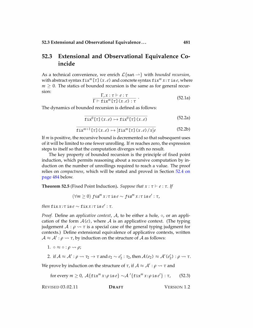
52.3 Extensional and Observational Equivalence . . . 481
52.3 Extensional and Observational Equivalence Co-incide
As a technical convenience, we enrich L{nat"} with bounded recursion,with abstract syntax fixm["](x.e) and concrete syntax fixm x:" is e, wherem 7 0. The statics of bounded recursion is the same as for general recur-sion:
!, x : " ) e : "! ) fixm["](x.e) : "
. (52.1a)
The dynamics of bounded recursion is defined as follows:
fix0["](x.e) 53 fix0["](x.e) (52.2a)
fixm+1["](x.e) 53 [fixm["](x.e)/x]e (52.2b)
If m is positive, the recursive bound is decremented so that subsequent usesof it will be limited to one fewer unrolling. If m reaches zero, the expressionsteps to itself so that the computation diverges with no result.
The key property of bounded recursion is the principle of fixed pointinduction, which permits reasoning about a recursive computation by in-duction on the number of unrollings required to reach a value. The proofrelies on compactness, which will be stated and proved in Section 52.4 onpage 484 below.
Theorem 52.5 (Fixed Point Induction). Suppose that x : " ) e : ". If
(&m 7 0) fixm x:" is e I fixm x:" is e% : ",
then fix x:" is e I fix x:" is e% : ".
Proof. Define an applicative context, A, to be either a hole, 8, or an appli-cation of the form A(e), where A is an applicative context. (The typingjudgement A : , ! " is a special case of the general typing judgment forcontexts.) Define extensional equivalence of applicative contexts, writtenA = A% : , ! ", by induction on the structure of A as follows:
1. 8 = 8 : , ! ,;
2. if A = A% : , ! "2 3 " and e2 I e%2 : "2, then A(e2) = A%(e%2) : , ! ".
We prove by induction on the structure of ", if A = A% : , ! " and
for every m 7 0, A{fixm x:, is e} IA %{fixm x:, is e%} : ", (52.3)
REVISED 03.02.11 DRAFT VERSION 1.2
482 52.3 Extensional and Observational Equivalence . . .
thenA{fix x:, is e} IA %{fix x:, is e%} : ". (52.4)
Choosing A = A% = 8 (so that , = ") completes the proof.If " = nat, then assume that A = A% : , ! nat and (52.3). By Defini-
tion 52.3 on page 480, we are to show
A{fix x:, is e} PA %{fix x:, is e%}.
By Corollary 52.14 on page 487 there exists m 7 0 such that
A{fix x:, is e} P A{fixm x:, is e}.
By (52.3) we have
A{fixm x:, is e} PA %{fixm x:, is e%}.
By Corollary 52.14 on page 487
A%{fixm x:, is e%} PA %{fix x:, is e%}.
The result follows by transitivity of Kleene equivalence.If " = "1 " "2, then by Definition 52.3 on page 480, it is enough to show
A{fix x:, is e}(e1) I A%{fix x:, is e%}(e%1) : "2
whenever e1 I e%1 : "1. Let A2 = A(e1) and A%2 = A%(e%1). It follows
from (52.3) that for every m 7 0
A2{fixm x:, is e} IA %2{fixm x:, is e%} : "2.
Noting that A2 = A%2 : , ! "2, we have by induction
A2{fix x:, is e} IA %2{fix x:, is e%} : "2,
as required.
Lemma 52.6 (Reflexivity). If ! ) e : ", then e I e : " [!].
Proof. The proof proceeds along the same lines as the proof of Theorem 51.8on page 473. The main difference is the treatment of general recursion,which is proved by fixed point induction. Consider Rule (13.1g). Assuming/ I /% : !, we are to show that
fix x:" is /(e) I fix x:" is )/%(e) : ".
VERSION 1.2 DRAFT REVISED 03.02.11
52.3 Extensional and Observational Equivalence . . . 483
By Theorem 52.5 on page 481 it is enough to show that, for every m 7 0,
fixm x:" is /(e) I fixm x:" is )/%(e) : ".
We proceed by an inner induction on m. When m = 0 the result is imme-diate, since both sides of the desired equivalence diverge. Assuming theresult for m, and applying Lemma 52.4 on page 480, it is enough to showthat /(e1) I )/%(e1) : ", where
e1 = [fixm x:" is /(e)/x]/(e), and (52.5)
e%1 = [fixm x:" is )/%(e)/x] )/%(e). (52.6)
But this follows directly from the inner and outer inductive hypotheses.For by the outer inductive hypothesis, if
fixm x:" is /(e) I fixm x:" is )/%(e) : ",
then
[fixm x:" is /(e)/x]/(e) I [fixm x:" is )/%(e)/x] )/%(e) : ".
But the hypothesis holds by the inner inductive hypothesis, from which theresult follows.
Symmetry and transitivity of eager extensional equivalence are easilyestablished by induction on types, noting that Kleene equivalence is sym-metric and transitive. Eager extensional equivalence is therefore an equiv-alence relation.
Lemma 52.7 (Congruence). If C0 : (! $ ") ! (!0 $ "0), and e I e% : " [!], thenC0{e} IC 0{e%} : "0 [!0].
Proof. By induction on the derivation of the typing of C0, following alongsimilar lines to the proof of Lemma 52.6 on the preceding page.
Logical equivalence is consistent, by definition. Consequently, it is con-tained in observational equivalence.
Theorem 52.8. If e I e% : " [!], then e I= e% : " [!].
Proof. By consistency and congruence of extensional equivalence.
Lemma 52.9. If e I= e% : ", then e I e% : ".
REVISED 03.02.11 DRAFT VERSION 1.2
484 52.4 Compactness
Proof. By induction on the structure of ". If " = nat, then the result is im-mediate, since the empty expression context is a program context. If " ="1 3 "2, then suppose that e1 I e%1 : "1. We are to show that e(e1) I e%(e%1) :"2. By Theorem 52.8 on the preceding page e1 I= e%1 : "1, and hence byLemma 52.2 on page 480 e(e1) I= e%(e%1) : "2, from which the result followsby induction.
Theorem 52.10. If e I= e% : " [!], then e I e% : " [!].
Proof. Assume that e I= e% : " [!]. Suppose that / I /% : !. By Theo-rem 52.8 on the preceding page we have / I= /% : !, and so by Lemma 52.2on page 480 we have
/(e) I= /%(e%) : ".
Therefore by Lemma 52.9 on the preceding page we have
/(e) I /%(e%) : ".
Corollary 52.11. e I= e% : " [!] iff e I e% : " [!].
52.4 Compactness
The principle of fixed point induction is derived from a critical property ofL{nat"}, called compactness. This property states that only finitely manyunwindings of a fixed point expression are needed in a complete evaluationof a program. While intuitively obvious (one cannot complete infinitelymany recursive calls in a finite computation), it is rather tricky to state andprove rigorously.
The proof of compactness (Theorem 52.13 on page 486) makes use ofthe stack machine for L{nat"} defined in Chapter 31, augmented withthe following transitions for bounded recursive expressions:
k $ fix0 x:" is e 53 k $ fix0 x:" is e (52.7a)
k $ fixm+1 x:" is e 53 k $ [fixm x:" is e/x]e (52.7b)
It is straightforward to extend the proof of correctness of the stack machine(Corollary 31.4 on page 271) to account for bounded recursion.
VERSION 1.2 DRAFT REVISED 03.02.11
52.4 Compactness 485
To get a feel for what is involved in the compactness proof, considerfirst the factorial function, f , in L{nat"}:
fix f:nat" nat is! (x:nat. ifz x {z; s(z) | s(x%); x 1 f(x%)}).
Obviously evaluation of f(n) requires n recursive calls to the function it-self. This means that, for a given input, n, we may place a bound, m, on therecursion that is sufficient to ensure termination of the computation. Thiscan be expressed formally using the m-bounded form of general recursion,
fixm f:nat" nat is! (x:nat. ifz x {z; s(z) | s(x%); x 1 f(x%)}).
Call this expression f (m). It follows from the definition of f that if f(n) 531
p, then f (m)(n) 531 p for some m 7 0 (in fact, m = n suffices).When considering expressions of higher type, we cannot expect to get
the same result from the bounded recursion as from the unbounded. Forexample, consider the addition function, a, of type " = nat" (nat" nat),given by the expression
fix p:" is! (x:nat. ifz x {z; id | s(x%); s 8 (p(x%))}),
where id = ! (y:nat. y) is the identity, e% 8 e = ! (x:". e%(e(x))) is compo-sition, and s = ! (x:nat. s(x)) is the successor function. The applicationa(n) terminates after three transitions, regardless of the value of n, result-ing in a !-abstraction. When n is positive, the result contains a residual copyof a itself, which is applied to n $ 1 as a recursive call. The m-bounded ver-sion of a, written a(m), is also such that a(m)() terminates in three steps,provided that m > 0. But the result is not the same, because the residualsof a appear as a(m$1), rather than as a itself.
Turning now to the proof of compactness, it is helpful to introduce somenotation. Suppose that x : " ) ex : " for some arbitrary abstractor x.ex.Define f ()) = fix x:" is ex, and f (m) = fixm x:" is ex, and observe thatf ()) : " and f (m) : " for any m 7 0.
The following technical lemma governing the stack machine permitsthe bound on “passive” occurrences of a recursive expression to be raisedwithout affecting the outcome of evaluation.
Lemma 52.12. If [ f (m)/y]k $ [ f (m)/y]e 531 % # n, where e ,= y, then [ f (m+1)/y]k $[ f (m+1)/y]e 531 % # n.
Proof. By induction on the definition of the transition judgement for K{nat"}.
REVISED 03.02.11 DRAFT VERSION 1.2
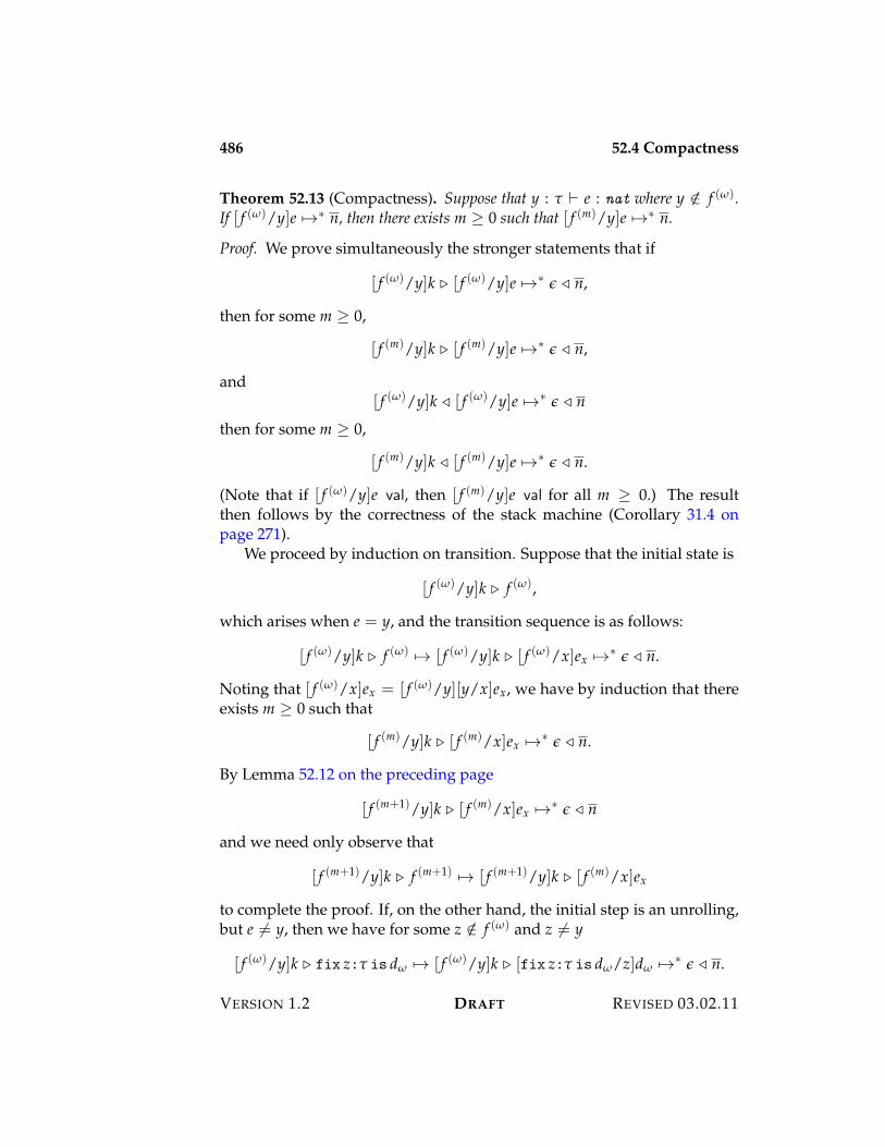
486 52.4 Compactness
Theorem 52.13 (Compactness). Suppose that y : " ) e : nat where y /+ f ()).If [ f ())/y]e 531 n, then there exists m 7 0 such that [ f (m)/y]e 531 n.
Proof. We prove simultaneously the stronger statements that if
[ f ())/y]k $ [ f ())/y]e 531 % # n,
then for some m 7 0,
[ f (m)/y]k $ [ f (m)/y]e 531 % # n,
and[ f ())/y]k # [ f ())/y]e 531 % # n
then for some m 7 0,
[ f (m)/y]k # [ f (m)/y]e 531 % # n.
(Note that if [ f ())/y]e val, then [ f (m)/y]e val for all m 7 0.) The resultthen follows by the correctness of the stack machine (Corollary 31.4 onpage 271).
We proceed by induction on transition. Suppose that the initial state is
[ f ())/y]k $ f ()),
which arises when e = y, and the transition sequence is as follows:
[ f ())/y]k $ f ()) 53 [ f ())/y]k $ [ f ())/x]ex 531 % # n.
Noting that [ f ())/x]ex = [ f ())/y][y/x]ex, we have by induction that thereexists m 7 0 such that
[ f (m)/y]k $ [ f (m)/x]ex 531 % # n.
By Lemma 52.12 on the preceding page
[ f (m+1)/y]k $ [ f (m)/x]ex 531 % # n
and we need only observe that
[ f (m+1)/y]k $ f (m+1) 53 [ f (m+1)/y]k $ [ f (m)/x]ex
to complete the proof. If, on the other hand, the initial step is an unrolling,but e ,= y, then we have for some z /+ f ()) and z ,= y
[ f ())/y]k $ fix z:" is d) 53 [ f ())/y]k $ [fix z:" is d)/z]d) 531 % # n.
VERSION 1.2 DRAFT REVISED 03.02.11
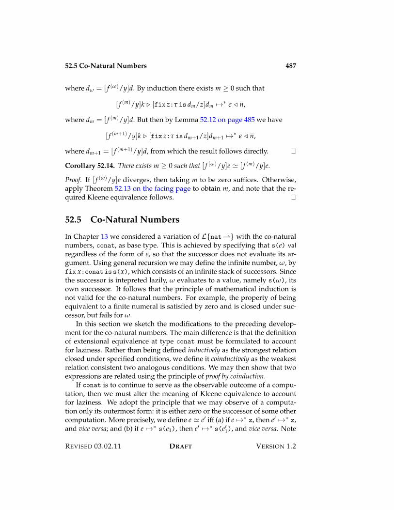
52.5 Co-Natural Numbers 487
where d) = [ f ())/y]d. By induction there exists m 7 0 such that
[ f (m)/y]k $ [fix z:" is dm/z]dm 531 % # n,
where dm = [ f (m)/y]d. But then by Lemma 52.12 on page 485 we have
[ f (m+1)/y]k $ [fix z:" is dm+1/z]dm+1 531 % # n,
where dm+1 = [ f (m+1)/y]d, from which the result follows directly.
Corollary 52.14. There exists m 7 0 such that [ f ())/y]e P [ f (m)/y]e.
Proof. If [ f ())/y]e diverges, then taking m to be zero suffices. Otherwise,apply Theorem 52.13 on the facing page to obtain m, and note that the re-quired Kleene equivalence follows.
52.5 Co-Natural Numbers
In Chapter 13 we considered a variation of L{nat"} with the co-naturalnumbers, conat, as base type. This is achieved by specifying that s(e) valregardless of the form of e, so that the successor does not evaluate its ar-gument. Using general recursion we may define the infinite number, ), byfix x:conat is s(x), which consists of an infinite stack of successors. Sincethe successor is intepreted lazily, ) evaluates to a value, namely s()), itsown successor. It follows that the principle of mathematical induction isnot valid for the co-natural numbers. For example, the property of beingequivalent to a finite numeral is satisfied by zero and is closed under suc-cessor, but fails for ).
In this section we sketch the modifications to the preceding develop-ment for the co-natural numbers. The main difference is that the definitionof extensional equivalence at type conat must be formulated to accountfor laziness. Rather than being defined inductively as the strongest relationclosed under specified conditions, we define it coinductively as the weakestrelation consistent two analogous conditions. We may then show that twoexpressions are related using the principle of proof by coinduction.
If conat is to continue to serve as the observable outcome of a compu-tation, then we must alter the meaning of Kleene equivalence to accountfor laziness. We adopt the principle that we may observe of a computa-tion only its outermost form: it is either zero or the successor of some othercomputation. More precisely, we define e P e% iff (a) if e 531 z, then e% 531 z,and vice versa; and (b) if e 531 s(e1), then e% 531 s(e%1), and vice versa. Note
REVISED 03.02.11 DRAFT VERSION 1.2
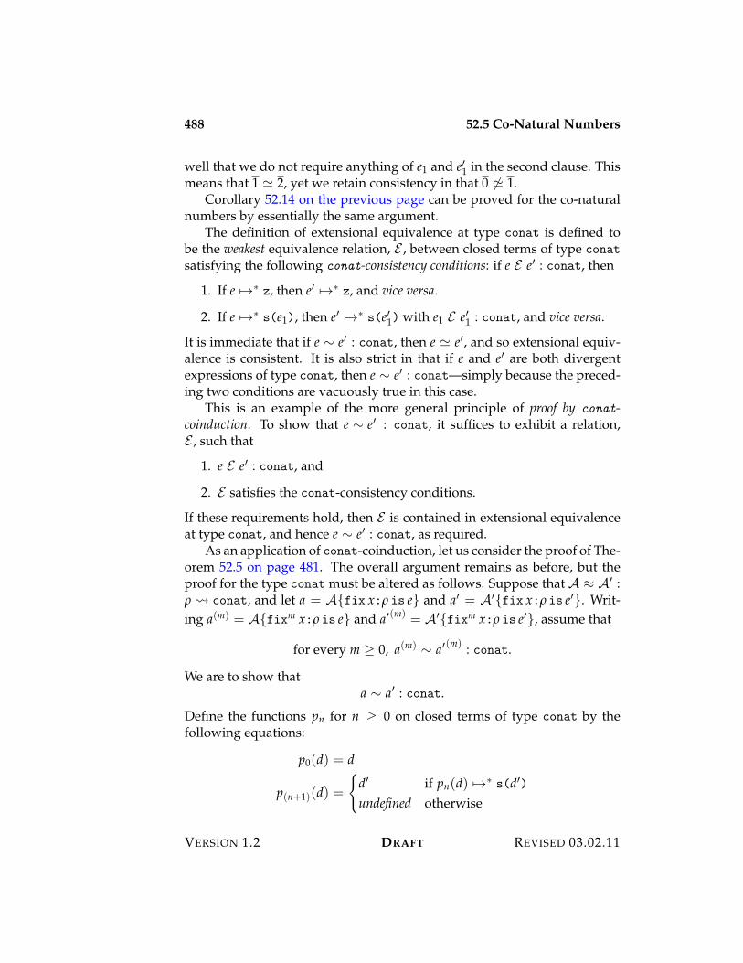
488 52.5 Co-Natural Numbers
well that we do not require anything of e1 and e%1 in the second clause. Thismeans that 1 P 2, yet we retain consistency in that 0 ,P 1.
Corollary 52.14 on the previous page can be proved for the co-naturalnumbers by essentially the same argument.
The definition of extensional equivalence at type conat is defined tobe the weakest equivalence relation, E , between closed terms of type conat
satisfying the following conat-consistency conditions: if e E e% : conat, then
1. If e 531 z, then e% 531 z, and vice versa.
2. If e 531 s(e1), then e% 531 s(e%1) with e1 E e%1 : conat, and vice versa.
It is immediate that if e I e% : conat, then e P e%, and so extensional equiv-alence is consistent. It is also strict in that if e and e% are both divergentexpressions of type conat, then e I e% : conat—simply because the preced-ing two conditions are vacuously true in this case.
This is an example of the more general principle of proof by conat-coinduction. To show that e I e% : conat, it suffices to exhibit a relation,E , such that
1. e E e% : conat, and
2. E satisfies the conat-consistency conditions.
If these requirements hold, then E is contained in extensional equivalenceat type conat, and hence e I e% : conat, as required.
As an application of conat-coinduction, let us consider the proof of The-orem 52.5 on page 481. The overall argument remains as before, but theproof for the type conat must be altered as follows. Suppose that A = A% :, ! conat, and let a = A{fix x:, is e} and a% = A%{fix x:, is e%}. Writ-ing a(m) = A{fixm x:, is e} and a%(m) = A%{fixm x:, is e%}, assume that
for every m 7 0, a(m) I a%(m) : conat.
We are to show thata I a% : conat.
Define the functions pn for n 7 0 on closed terms of type conat by thefollowing equations:
p0(d) = d
p(n+1)(d) =
%d% if pn(d) 531 s(d%)undefined otherwise
VERSION 1.2 DRAFT REVISED 03.02.11
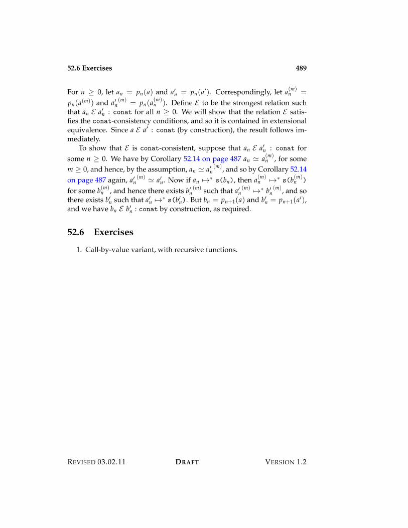
52.6 Exercises 489
For n 7 0, let an = pn(a) and a%n = pn(a%). Correspondingly, let a(m)n =
pn(a(m)) and a%n(m) = pn(a(m)
n ). Define E to be the strongest relation suchthat an E a%n : conat for all n 7 0. We will show that the relation E satis-fies the conat-consistency conditions, and so it is contained in extensionalequivalence. Since a E a% : conat (by construction), the result follows im-mediately.
To show that E is conat-consistent, suppose that an E a%n : conat forsome n 7 0. We have by Corollary 52.14 on page 487 an P a(m)
n , for somem 7 0, and hence, by the assumption, an P a%n
(m), and so by Corollary 52.14on page 487 again, a%n
(m) P a%n. Now if an 531 s(bn), then a(m)n 531 s(b(m)
n )
for some b(m)n , and hence there exists b%n
(m) such that a%n(m) 531 b%n
(m), and sothere exists b%n such that a%n 531 s(b%n). But bn = pn+1(a) and b%n = pn+1(a%),and we have bn E b%n : conat by construction, as required.
52.6 Exercises
1. Call-by-value variant, with recursive functions.
REVISED 03.02.11 DRAFT VERSION 1.2

490 52.6 Exercises
VERSION 1.2 DRAFT REVISED 03.02.11
Chapter 53
Parametricity
The motivation for introducing polymorphism was to enable more pro-grams to be written — those that are “generic” in one or more types, suchas the composition function given in Chapter 23. Then if a program doesnot depend on the choice of types, we can code it using polymorphism.Moreover, if we wish to insist that a program can not depend on a choiceof types, we demand that it be polymorphic. Thus polymorphism can beused both to expand the collection of programs we may write, and also tolimit the collection of programs that are permissible in a given context.
The restrictions imposed by polymorphic typing give rise to the expe-rience that in a polymorphic functional language, if the types are correct,then the program is correct. Roughly speaking, if a function has a poly-morphic type, then the strictures of type genericity vastly cut down the setof programs with that type. Thus if you have written a program with thistype, it is quite likely to be the one you intended!
The technical foundation for these remarks is called parametricity. Thegoal of this chapter is to give an account of parametricity for L{3&} undera call-by-name interpretation.
53.1 Overview
We will begin with an informal discussion of parametricity based on a “seatof the pants” understanding of the set of well-formed programs of a type.
Suppose that a function value f has the type &(t.t 3 t). What functioncould it be? When instantiated at a type " it should evaluate to a functiong of type " 3 " that, when further applied to a value v of type " returnsa value v% of type ". Since f is polymorphic, g cannot depend on v, so v%
492 53.2 Observational Equivalence
must be v. In other words, g must be the identity function at type ", and fmust therefore be the polymorphic identity.
Suppose that f is a function of type &(t.t). What function could it be?A moment’s thought reveals that it cannot exist at all! For it must, wheninstantiated at a type ", return a value of that type. But not every type hasa value (including this one), so this is an impossible assignment. The onlyconclusion is that &(t.t) is an empty type.
Let N be the type of polymorphic Church numerals introduced in Chap-ter 23, namely &(t.t 3 (t 3 t) 3 t). What are the values of this type?Given any type ", and values z : " and s : " 3 ", the expression
f["](z)(s)
must yield a value of type ". Moreover, it must behave uniformly withrespect to the choice of ". What values could it yield? The only way tobuild a value of type " is by using the element z and the function s passedto it. A moment’s thought reveals that the application must amount to then-fold composition
s(s(. . . s(z) . . .)).
That is, the elements of N are in one-to-one correspondence with the natu-ral numbers.
53.2 Observational Equivalence
The definition of observational equivalence given in Chapters 51 and 52 isbased on identifying a type of answers that are observable outcomes of com-plete programs. Values of function type are not regarded as answers, butare treated as “black boxes” with no internal structure, only input-outputbehavior. In L{3&}, however, there are no (closed) base types! Every typeis either a function type or a polymorphic type, and hence no types suitableto serve as observable answers.
One way to manage this difficulty is to augment L{3&} with a basetype of answers to serve as the observable outcomes of a computation. Theonly requirement is that this type have two elements that can be immedi-ately distinguished from each other by evaluation. We may achieve thisby enriching L{3&} with a base type, 2, containing two constants, tt andff, that serve as possible answers for a complete computation. A completeprogram is a closed expression of type 2.
Kleene equivalence is defined for complete programs by requiring thate P e% iff either (a) e 531 tt and e% 531 tt; or (b) e 531 ff and e% 531 ff.
VERSION 1.2 DRAFT REVISED 03.02.11
53.2 Observational Equivalence 493
This is obviously an equivalence relation, and it is immediate that tt ,Pff, since these are two distinct constants. As before, we say that a type-indexed family of equivalence relations between closed expressions of thesame type is consistent if it implies Kleene equivalence at the answer type,2.
To define observational equivalence, we must first define the concept ofan expression context for L{3&} as an expression with a “hole” in it. Moreprecisely, we may give an inductive definition of the judgement
C : ("; ! $ ") ! ("%; !% $ "%),
which states that C is an expression context that, when filled with an ex-pression "; ! ) e : " yields an expression "%; !% ) C{e} : ". (We leave theprecise definition of this judgement, and the verification of its properties,as an exercise for the reader.)
Definition 53.1. Two expressions of the same type are observationally equiva-lent, written e I= e% : " ["; !], iff C{e} P C{e%} whenever C : ("; ! $ ") ! (# $ 2).
Lemma 53.1. Observational equivalence is the coarsest consistent congruence.
Proof. The composition of a program context with another context is itselfa program context. It is consistent by virtue of the empty context being aprogram context.
Lemma 53.2.
1. If e I= e% : " [", t; !] and , type, then [,/t]e I= [,/t]e% : [,/t]" ["; [,/t]!].
2. If e I= e% : " [#; !, x : &] and d : &, then [d/x]e I= [d/x]e% : " [#; !]. More-over, if d I= d% : &, then [d/x]e I= [d%/x]e : " [#; !] and [d/x]e% I= [d%/x]e% :" [#; !].
Proof. 1. Let C : ("; [,/t]! $ [,/t]") ! (# $ 2) be a program context. Weare to show that
C{[,/t]e} P C{[,/t]e%}.
Since C is closed, this is equivalent to
[,/t]C{e} P [,/t]C{e%}.
Let C % be the context ((t.C{8})[,], and observe that
C % : (", t; ! $ ") ! (# $ 2).
REVISED 03.02.11 DRAFT VERSION 1.2
494 53.3 Logical Equivalence
Therefore, from the assumption,
C %{e} PC %{e%}.
But C %{e} P [,/t]C{e}, and C %{e%} P [,/t]C{e%}, from which the re-sult follows.
2. By an argument essentially similar to that for Lemma 51.5 on page 471.
53.3 Logical Equivalence
In this section we introduce a form of logical equivalence that captures theinformal concept of parametricity, and also provides a characterization ofobservational equivalence. This will permit us to derive properties of ob-servational equivalence of polymorphic programs of the kind suggestedearlier.
The definition of logical equivalence for L{3&} is somewhat morecomplex than for L{nat3}. The main idea is to define logical equiva-lence for a polymorphic type, &(t.") to satisfy a very strong condition thatcaptures the essence of parametricity. As a first approximation, we mightsay that two expressions, e and e%, of this type should be logically equiva-lent if they are logically equivalent for “all possible” interpretations of thetype t. More precisely, we might require that e[,] be related to e%[,] attype [,/t]", for any choice of type ,. But this runs into two problems, onetechnical, the other conceptual. The same device will be used to solve bothproblems.
The technical problem stems from impredicativity. In Chapter 51 logi-cal equivalence is defined by induction on the structure of types. But whenpolymorphism is impredicative, the type [,/t]" might well be larger than&(t.")! At the very least we would have to justify the definition of logicalequivalence on some other grounds, but no criterion appears to be avail-able. The conceptual problem is that, even if we could make sense of thedefinition of logical equivalence, it would be too restrictive. For such a def-inition amounts to saying that the unknown type t is to be interpreted aslogical equivalence at whatever type it turns out to be when instantiated.To obtain useful parametricity results, we shall ask for much more thanthis. What we shall do is to consider separately instances of e and e% by types, and ,%, and treat the type variable t as standing for any relation (of someform) between , and ,%. One may suspect that this is asking too much: per-haps logical equivalence is the empty relation! Surprisingly, this is not the
VERSION 1.2 DRAFT REVISED 03.02.11
53.3 Logical Equivalence 495
case, and indeed it is this very feature of the definition that we shall exploitto derive parametricity results about the language.
To manage both of these problems we will consider a generalization oflogical equivalence that is parameterized by a relational interpretation ofthe free type variables of its classifier. The parameters determine a sepa-rate binding for each free type variable in the classifier for each side of theequation, with the discrepancy being mediated by a specified relation be-tween them. This permits us to consider a notion of “equivalence” betweentwo expressions of different type—they are equivalent, modulo a relationbetween the interpretations of their free type variables.
We will restrict attention to a certain collection of “admissible” binaryrelations between closed expressions. The conditions are imposed to ensurethat logical equivalence and observational equivalence coincide.
Definition 53.2 (Admissibility). A relation R between expressions of types ,and ,% is admissible, written R : , . ,%, iff it satisfies two requirements:
1. Respect for observational equivalence: if R(e, e%) and d I= e : , and d% I= e% :,%, then R(d, d%).
2. Closure under converse evaluation: if R(e, e%), then if d 53 e, then R(d, e%)and if d% 53 e%, then R(e, d%).
The second of these conditions will turn out to be a consequence of the first,but we are not yet in a position to establish this fact.
The judgement 2 : " states that 2 is a type substitution that assigns aclosed type to each type variable t + ". A type substitution, 2, induces asubstitution function, 2, on types given by the equation
2(") = [2(t1), . . . , 2(tn)/t1, . . . , tn]",
and similarly for expressions. Substitution is extended to contexts point-wise by defining 2(!)(x) = 2(!(x)) for each x + dom(!).
Let 2 and 2% be two type substitutions of closed types to the type vari-ables in ". A relation assignment, 3, between 2 and 2% is an assignment ofan admissible relation 3(t) : 2(t) . 2%(t) to each t + ". The judgement3 : 2 . 2% states that 3 is a relation assignment between 2 and 2%.
Logical equivalence is defined in terms of its generalization, called para-metric logical equivalence, written e I e% : " [3 : 2 . 2%], defined as follows.
REVISED 03.02.11 DRAFT VERSION 1.2
496 53.3 Logical Equivalence
Definition 53.3 (Parametric Logical Equivalence). The relation e I e% : " [3 :2 . 2%] is defined by induction on the structure of " by the following conditions:
e I e% : t [3 : 2 . 2%] iff 3(t)(e, e%)e I e% : 2 [3 : 2 . 2%] iff e P e%e I e% : "1 3 "2 [3 : 2 . 2%] iff e1 I e%1 : "1 [3 : 2 . 2%] implies
e(e1) I e%(e%1) : "2 [3 : 2 . 2%]e I e% : &(t.") [3 : 2 . 2%] iff for every ,, ,%, and every R : , . ,%,
e[,] I e%[,%] : " [3[t 53 R] : 2[t 53 ,] . 2%[t 53 ,%]]
Logical equivalence is defined in terms of parametric logical equiva-lence by considering all possible interpretations of its free type- and ex-pression variables. An expression substitution, /, for a context !, written/ : !, is an substitution of a closed expression /(x) : !(x) to each vari-able x + dom(!). An expression substitution, / : !, induces a substitutionfunction, /, defined by the equation
/(e) = [/(x1), . . . , /(xn)/x1, . . . , xn]e,
where the domain of ! consists of the variables x1, . . . , xn. The relation/ I /% : ! [3 : 2 . 2%] is defined to hold iff dom(/) = dom(/%) = dom(!),and /(x) I /%(x) : !(x) [3 : 2 . 2%] for every variable, x, in their commondomain.
Definition 53.4 (Logical Equivalence). The expressions "; ! ) e : " and "; ! )e% : " are logically equivalent, written e I e% : " ["; !] iff for every assigment2 and 2% of closed types to type variables in ", and every relation assignment 3 :2 . 2%, if / I /% : ! [3 : 2 . 2%], then /(2(e)) I )/%()2%(e%)) : " [3 : 2 . 2%].
When e, e%, and " are closed, then this definition states that e I e% : " iffe I e% : " [# : # . #], so that logical equivalence is indeed a special caseof its generalization.
Lemma 53.3 (Closure under Converse Evaluation). Suppose that e I e% :" [3 : 2 . 2%]. If d 53 e, then d I e% : ", and if d% 53 e%, then e I d% : ".
Proof. By induction on the structure of ". When " = t, the result holds bythe definition of admissibility. Otherwise the result follows by induction,making use of the definition of the transition relation for applications andtype applications.
Lemma 53.4 (Respect for Observational Equivalence). Suppose that e I e% :" [3 : 2 . 2%]. If d I= e : 2(") and d% I= e% : )2%("), then d I d% : " [3 : 2 . 2%].
VERSION 1.2 DRAFT REVISED 03.02.11
53.3 Logical Equivalence 497
Proof. By induction on the structure of ", relying on the definition of ad-missibility, and the congruence property of observational equivalence. Forexample, if " = &(t.&), then we are to show that for every R : , . ,%,
d[,] I d%[,%] : & [3[t 53 R] : 2[t 53 ,] . 2%[t 53 ,%]].
Since observational equivalence is a congruence, d[,] I= e[,] : [,/t]2(&),d%[,] I= e%[,] : [,%/t])2%(&). From the assumption it follows that
e[,] I e%[,%] : & [3[t 53 R] : 2[t 53 ,] . 2%[t 53 ,%]],
from which the result follows by induction.
Corollary 53.5. The relation e I e% : " [3 : 2 . 2%] is an admissible relationbetween closed types 2(") and )2%(").
Proof. By Lemmas 53.3 on the facing page and 53.4 on the preceding page.
Corollary 53.6. If e I e% : " ["; !], and d I= e : " ["; !] and d% I= e% : " ["; !],then d I d% : " ["; !].
Proof. By Lemma 53.2 on page 493 and Corollary 53.5.
Lemma 53.7 (Compositionality). Suppose that
e I e% : " [3[t 53 R] : 2[t 53 2(,)] . 2%[t 53 )2%(,)]],
where R : 2(,) . )2%(,) is such that R(d, d%) holds iff d I d% : , [3 : 2 . 2%].Then e I e% : [,/t]" [3 : 2 . 2%].
Proof. By induction on the structure of ". When " = t, the result is imme-diate from the definition of the relation R. When " = t% ,= t, the resultholds vacuously. When " = "1 3 "2 or " = &(u."), where without loss ofgenerality u ,= t and u /+ ,, the result follows by induction.
Despite the strong conditions on polymorphic types, logical equiva-lence is not overly restrictive—every expression satisfies its constraints.This result is sometimes called the parametricity theorem.
Theorem 53.8 (Parametricity). If "; ! ) e : ", then e I e : " ["; !].
Proof. By rule induction on the statics of L{3&} given by Rules (23.2).We consider two representative cases here.
REVISED 03.02.11 DRAFT VERSION 1.2
498 53.3 Logical Equivalence
Rule (23.2d) Suppose 2 : ", 2% : ", 3 : 2 . 2%, and / I /% : ! [3 : 2 . 2%].By induction we have that for all ,, ,%, and R : , . ,%,
[,/t]/(2(e)) I [,%/t] )/%()2%(e)) : " [31 : 21 . 2%1],
where 31 = 3[t 53 R], 21 = 2[t 53 ,], and 2%1 = 2%[t 53 ,%]. Since
((t./(2(e)))[,] 531 [,/t]/(2(e))
and((t. )/%()2%(e)))[,%] 531 [,%/t] )/%()2%(e)),
the result follows by Lemma 53.3 on page 496.
Rule (23.2e) Suppose 2 : ", 2% : ", 3 : 2 . 2%, and / I /% : ! [3 : 2 . 2%].By induction we have
/(2(e)) I )/%()2%(e)) : &(t.") [3 : 2 . 2%]
Let , = 2(,) and ,% = )2%(,). Define the relation R : , . ,% by R(d, d%)iff d I d% : , [3 : 2 . 2%]. By Corollary 53.5 on the previous page, thisrelation is admissible.
By the definition of logical equivalence at polymorphic types, we ob-tain
/(2(e))[,] I )/%()2%(e))[,%] : " [3[t 53 R] : 2[t 53 ,] . 2%[t 53 ,%]].
By Lemma 53.7 on the preceding page
/(2(e))[,] I )/%()2%(e))[,%] : [,/t]" [3 : 2 . 2%]
But
/(2(e))[,] = /(2(e))[2(,)] (53.1)
= /(2(e[,])), (53.2)
and similarly
)/%()2%(e))[,%] = )/%()2%(e))[)2%(,)] (53.3)
= )/%()2%(e[,])), (53.4)
from which the result follows.
VERSION 1.2 DRAFT REVISED 03.02.11
53.3 Logical Equivalence 499
Corollary 53.9. If e I= e% : " ["; !], then e I e% : " ["; !].
Proof. By Theorem 53.8 on page 497 e I e : " ["; !], and hence by Corol-lary 53.6 on page 497, e I e% : " ["; !].
Lemma 53.10 (Congruence). If e I e% : " ["; !] and C : ("; ! $ ") ! ("%; !% $ "%),then C{e} I C{e%} : " ["%; !%].
Proof. By induction on the structure of C, following along very similar linesto the proof of Theorem 53.8 on page 497.
Lemma 53.11 (Consistency). Logical equivalence is consistent.
Proof. Follows immediately from the definition of logical equivalence.
Corollary 53.12. If e I e% : " ["; !], then e I= e% : " ["; !].
Proof. By Lemma 53.11 Logical equivalence is consistent, and by Lemma 53.10,it is a congruence, and hence is contained in observational equivalence.
Corollary 53.13. Logical and observational equivalence coincide.
Proof. By Corollaries 53.9 and 53.12.
If d : " and d 53 e, then d I e : ", and hence by Corollary 53.12, d I= e : ".Therefore if a relation respects observational equivalence, it must also beclosed under converse evaluation. This shows that the second condition onadmissibility is redundant, now that we have established the coincidenceof logical and observational equivalence.
Corollary 53.14 (Extensionality).
1. e I= e% : "1 3 "2 iff for all e1 : "1, e(e1) I= e%(e1) : "2.
2. e I= e% : &(t.") iff for all ,, e[,] I= e%[,] : [,/t]".
Proof. The forward direction is immediate in both cases, since observa-tional equivalence is a congruence, by definition. The backward directionis proved similarly in both cases, by appeal to Theorem 53.8 on page 497. Inthe first case, by Corollary 53.13 it suffices to show that e I e% : "1 3 "2. Tothis end suppose that e1 I e%1 : "1. We are to show that e(e1) I e%(e%1) : "2.By the assumption we have e(e%1) I= e%(e%1) : "2. By parametricity we havee I e : "1 3 "2, and hence e(e1) I e(e%1) : "2. The result then follows
REVISED 03.02.11 DRAFT VERSION 1.2
500 53.4 Parametricity Properties
by Lemma 53.4 on page 496. In the second case, by Corollary 53.13 onthe preceding page it is sufficient to show that e I e% : &(t."). Supposethat R : , . ,% for some closed types , and ,%. It suffices to show thate[,] I e%[,%] : " [3 : 2 . 2%], where 3(t) = R, 2(t) = ,, and 2%(t) = ,%. Bythe assumption we have e[,%] I= e%[,%] : [,/t]". By parametricity e I e :&(t."), and hence e[,] I e%[,%] : " [3 : 2 . 2%]. The result then follows byLemma 53.4 on page 496.
Lemma 53.15 (Identity Extension). Let 3 : 2 . 2 be such that 3(t) is observa-tional equivalence at type 2(t) for each t + dom(2). Then e I e% : " [3 : 2 . 2]iff e I= e% : 2(").
Proof. The backward direction follows immediately from Theorem 53.8 onpage 497 and respect for observational equivalence. The forward directionis proved by induction on the structure of ", appealing to Corollary 53.14on the previous page to establish observational equivalence at function andpolymorphic types.
53.4 Parametricity Properties
The parametricity theorem enables us to deduce properties of expressionsof L{3&} that hold solely because of their type. The stringencies of para-metricity ensure that a polymorphic type has very few inhabitants. Forexample, we may prove that every expression of type &(t.t 3 t) behaveslike the identity function.
Theorem 53.16. Let e : &(t.t 3 t) be arbitrary, and let id be ((t.! (x:t. x)).Then e I= id : &(t.t 3 t).
Proof. By Corollary 53.13 on the preceding page it is sufficient to show thate I id : &(t.t 3 t). Let , and ,% be arbitrary closed types, let R : , . ,% bean admissible relation, and suppose that e0 R e%0. We are to show
e[,](e0) R id[,](e%0),
which, given the definition of id, is to say
e[,](e0) R e%0.
It suffices to show that e[,](e0) I= e0 : ,, for then the result follows by theadmissibility of R and the assumption e0 R e%0.
VERSION 1.2 DRAFT REVISED 03.02.11
53.4 Parametricity Properties 501
By Theorem 53.8 on page 497 we have e I e : &(t.t 3 t). Let the re-lation S : , . , be defined by d S d% iff d I= e0 : , and d% I= e0 : ,. This isclearly admissible, and we have e0 S e0. It follows that
e[,](e0) S e[,](e0),
and so, by the definition of the relation S, e[,](e0) I= e0 : ,.
In Chapter 23 we showed that product, sum, and natural numbers typesare all definable in L{3&}. The proof of definability in each case consistedof showing that the type and its associated introduction and eliminationforms are encodable in L{3&}. The encodings are correct in the (weak)sense that the dynamics of these constructs as given in the earlier chaptersis derivable from the dynamics of L{3&} via these definitions. By takingadvantage of parametricity we may extend these results to obtain a strongcorrespondence between these types and their encodings.
As a first example, let us consider the representation of the unit type,unit, in L{3&}, as defined in Chapter 23 by the following equations:
unit = &(r.r 3 r)?@ = ((r.! (x:r. x))
It is easy to see that ?@ : unit according to these definitions. But this merelysays that the type unit is inhabited (has an element). What we would liketo know is that, up to observational equivalence, the expression ?@ is theonly element of that type. But this is precisely the content of Theorem 53.16on the facing page! We say that the type unit is strongly definable withinL{3&}.
Continuing in this vein, let us examine the definition of the binary prod-uct type in L{3&}, also given in Chapter 23:
"1 < "2 = &(r.("1 3 "2 3 r) 3 r)?e1, e2@ = ((r.! (x:"1 3 "2 3 r. x(e1)(e2)))
e · l = e["1](! (x:"1. ! (y:"2. x)))e · r = e["2](! (x:"1. ! (y:"2. y)))
It is easy to check that ?e1, e2@ · l I= e1 : "1 and ?e1, e2@ · r I= e2 : "2 by a directcalculation.
We wish to show that the ordered pair, as defined above, is the uniquesuch expression, and hence that Cartesian products are strongly definable
REVISED 03.02.11 DRAFT VERSION 1.2
502 53.4 Parametricity Properties
in L{3&}. We will make use of a lemma governing the behavior of the ele-ments of the product type whose proof relies on Theorem 53.8 on page 497.
Lemma 53.17. If e : "1 < "2, then e I= ?e1, e2@ : "1 < "2 for some e1 : "1 ande2 : "2.
Proof. Expanding the definitions of pairing and the product type, and ap-plying Corollary 53.13 on page 499, we let , and ,% be arbitrary closed types,and let R : , . ,% be an admissible relation between them. Suppose furtherthat
h I h% : "1 3 "2 3 t [3 : 2 . 2%],
where 3(t) = R, 2(t) = ,, and 2%(t) = ,% (and are each undefined on t% ,= t).We are to show that for some e1 : "1 and e2 : "2,
e[,](h) I h%(e1)(e2) : t [3 : 2 . 2%],
which is to saye[,](h) R h%(e1)(e2).
Now by Theorem 53.8 on page 497 we have e I e : "1 < "2. Define therelation S : , . ,% by d S d% iff the following conditions are satisfied:
1. d I= h(d1)(d2) : , for some d1 : "1 and d2 : "2;
2. d% I= h%(d%1)(d%2) : ,% for some d%1 : "1 and d%2 : "2;
3. d R d%.
This is clearly an admissible relation. Noting that
h I h% : "1 3 "2 3 t [3% : 2 . 2%],
where 3%(t) = S and is undefined for t% ,= t, we conclude that e[,](h) Se[,%](h%), and hence
e[,](h) R h%(d%1)(d%2),
as required.
Now suppose that e : "1 < "2 is such that e · l I= e1 : "1 and e · r I= e2 : "2.We wish to show that e I= ?e1, e2@ : "1 < "2. From Lemma 53.17 it is easy todeduce that e I= ?e · l, e · r@ : "1 < "2 by congruence and direct calculation.Hence, by congruence we have e I= ?e1, e2@ : "1 < "2.
By a similar line of reasoning we may show that the Church encodingof the natural numbers given in Chapter 23 strongly defines the naturalnumbers in that the following properties hold:
VERSION 1.2 DRAFT REVISED 03.02.11
53.5 Representation Independence, Revisited 503
1. natiter z {z;e0 | s(x);e1} I= e0 : ,.
2. natiter s(e) {z;e0 | s(x);e1} I= [natiter e {z;e0 | s(x);e1}/x]e1 :,.
3. Suppose that x : nat ) r(x) : ,. If
(a) r(z) I= e0 : ,, and(b) r(s(e)) I= [r(e)/x]e1 : ,,
then for every e : nat, r(e) I= natiter e {z;e0 | s(x);e1} : ,.
The first two equations, which constitute weak definability, are easily estab-lished by calculation, using the definitions given in Chapter 23. The thirdproperty, the unicity of the iterator, is proved using parametricity by show-ing that every closed expression of type nat is observationally equivalentto a numeral n. We then argue for unicity of the iterator by mathematicalinduction on n 7 0.
Lemma 53.18. If e : nat, then either e I= z : nat, or there exists e% : nat suchthat e I= s(e%) : nat. Consequently, there exists n 7 0 such that e I= n : nat.
Proof. By Theorem 53.8 on page 497 we have e I e : nat. Define the relationR : nat . nat to be the strongest relation such that d R d% iff either d I= z :nat and d% I= z : nat, or d I= s(d1) : nat and d% I= s(d%1) : nat and d1 R d%1.It is easy to see that z R z, and if e R e%, then s(e) R s(e%). Letting zero = z
and succ = ! (x:nat. s(x)), we have
e[nat](zero)(succ) R e[nat](zero)(succ).
The result follows by the induction principle arising from the definition ofR as the strongest relation satisfying its defining conditions.
53.5 Representation Independence, Revisited
In Section 24.4 on page 213 we discussed the property of representation in-dependence for abstract types. This property states that if two implemen-tations of an abstract type are “similar”, then the client behavior is not af-fected by replacing one for the other. The crux of the matter is the definitionof similarity of two implementations. Informally, two implementations ofan abstract type are similar if there is a relation, E, between their represen-tation types that is preserved by the operations of the type. The relation E
REVISED 03.02.11 DRAFT VERSION 1.2
504 53.5 Representation Independence, Revisited
may be thought of as expressing the “equivalence” of the two representa-tions; checking that each operation preserves E amounts to checking thatthe result of performing that operation on equivalent representations yieldsequivalent results.
As an example, we argued in Section 24.4 on page 213 that two im-plementations of a queue abstraction are similar. In the one the queue isrepresented by a list of elements in reverse arrival order (the latest elementto arise is the head of the list). Enqueueing an element is easy; simply addit to the front of the list. Dequeueing an element requires reversing thelist, removing the first element, and reversing the rest to obtain the newqueue. In the other the queue is represented by a pair of lists, with the“back half” representing the latest arrivals in reverse order of arrival time,and the “front half” representing the oldest arrivals in order of arrival (thenext one to depart the queue is at the head of the list). Enqueueing remainseasy; the element is added to the “back half” as the first element. Dequeue-ing breaks into two cases. If the “front half” is non-empty, simply removethe head element and return the queue consisting of the “back half” as-istogether with the tail of the “front half”. If, on the other hand, the “fronthalf” is empty, then the queue is reorganizing by reversing the “back half”and making it the new “front half”, leaving the new “back half” empty.These two representations of queues are related by the relation E such thatq E (b, f ) iff q is b followed by the reversal of f . It is easy to check that theoperations of the queue preserve this relationship.
In Chapter 24 we asserted without proof that the existence of such arelation was sufficient to ensure that the behavior of any client is insensi-tive to the choice of either implementation. The proof of this intuitivelyplausible result relies on parametricity. One way to explain this is viathe definition of existential types in L{3&} described in Section 24.3 onpage 212. According to that definition, the client, e, of an abstract type'(t.") is a polymorphic function of type &(t." 3 &), where &, the re-sult type of the computation, does not involve the type variable t. Beingpolymorphic, the client enjoys the parametricity property given by Theo-rem 53.8 on page 497. Specifically, suppose that ,1 and ,2 are two closedrepresentation types and that R : ,1 . ,2 is an admissible relation betweenthem. For example, in the case of the queue abstraction, ,1 is the type oflists of elements of the queue, ,2 is the type of a pair of lists of elements,and R is the relation E given above. Suppose further that e1 : [,1/t]" ande2 : [,2/t]" are two implementations of the operations such that
e1 I e2 : " [3 : 21 . 22], (53.5)
VERSION 1.2 DRAFT REVISED 03.02.11

53.6 Exercises 505
where 3(t) = R, 21(t) = ,1, and 22(t) = ,2. In the case of the queues exam-ple the expression e1 is the implementation of the queue operations in termsof lists, and the e2 is the implementation in terms of pairs of lists describedearlier. Condition (53.5) states that the two implementations are similarin that they preserve the relation R between the representation types. ByTheorem 53.8 on page 497 it follows that the client, e, satisfies
e I e : & [3 : 21 . 22].
But since & is a closed type (in particular, does not involve t), this is equiv-alent to
e I e : & [# : # . #].
But then by Lemma 53.15 on page 500 we have
e[,1](e1) I= e[,2](e2) : &.
That is, the client behavior is not affected by the change of representation.
53.6 Exercises
REVISED 03.02.11 DRAFT VERSION 1.2

506 53.6 Exercises
VERSION 1.2 DRAFT REVISED 03.02.11

Part XX
Appendices

Appendix A
Mathematical Preliminaries
A.1 Finite Sets and Maps
A.2 Families of Sets

510 A.2 Families of Sets
VERSION 1.2 DRAFT REVISED 03.02.11
History of versions
Version Date Author(s) Changes
1.0 21.01.11 RH Created1.1 21.01.11 RH Concurrent and Distributed Algol1.2 03.02.11 RH Clarified discussion of rule induction.