Participatory Plant Breeding (Training Manual)

S. Ceccarelli

January 2010

1

Table of Contentsii. Foreword...................................................................................................4iii. Acknowledgement...................................................................................4iv. Acronyms.................................................................................................5

Introduction and Definitions......................................................................5Historical perspective...................................................................................5Plant breeding..............................................................................................7Participatory Plant Breeding (PPB)................................................................9Participatory Variety Selection (PVS)..........................................................11The Participatory Model of the ICARDA Barley Program.............................11

How to get started: organizational issues.............................................12Setting criteria to identify target environments and target users..............16Identification of the target environment and users....................................17Type of participation...................................................................................19Choice of parental material........................................................................19Choice of breeding method........................................................................19Naming of varieties....................................................................................21Management of trials in farmers’ fields......................................................22Farmer selection.........................................................................................25Visits to farmers.........................................................................................26Managing the transition phase...................................................................27Sharing and Dissemination of Findings.......................................................27

Data Collection...........................................................................................27Before Harvesting.......................................................................................29At Harvest...................................................................................................29After Harvest..............................................................................................29Derived data...............................................................................................29

Experimental designs for PPB trials.......................................................32Stage 1 trials..............................................................................................33Stage 2 and 3 trials....................................................................................37Stage 4 trials..............................................................................................39

Preparation of Data Files and Data Entry..............................................40Randomization............................................................................................43Preparation of a File for Data Recording.....................................................45

Unreplicated or partially replicated trials................................................45Replicated trials.......................................................................................46

Data Entry..................................................................................................47Data Storage..............................................................................................51

Data Analysis..............................................................................................51Updating a File for Data Analysis: unreplicated trials.................................51Spatial Analysis of an unreplicated trials....................................................52Updating a File for Data Analysis: replicated trials in rows and columns.. .54Spatial Analysis of a replicated trials in rows and columns........................54Updating a File for Data Analysis: replicated trials.....................................55

2

Spatial Analysis of a replicated trials..........................................................56Importing the Results of the Analysis......................................................58

Discussion of results and farmers’ final selection.......................................63Stage 1 trials...........................................................................................63Stage 2 trials...........................................................................................68Stage 3 trials...........................................................................................73Stage 4 trials...........................................................................................77

Genotype x Environment Interactions........................................................79GGE biplot...................................................................................................81

Genotype x Location Interactions in stage 1 trials..................................81Genotype x Location x Year Interactions in stage 2, 3 and 4 trials.........81Relationships between traits...................................................................81Farmers’ selection criteria.......................................................................81

References...................................................................................................82

3

ii. ForewordThis manual on Participatory Plant Breeding (PPB) is based firstly on the direct experience derived from several years of implementing PPB programs in a number of countries and on a number of crops, and secondly, when necessary, on relevant scientific literature. The methods presented here have been used in rural communities over the course of several, years particularly in North Africa (Tunisia, Morocco, Egypt and Algeria), the Horn of Africa (Eritrea), the Arabian Peninsula (Yemen) and the Near East (Syria, Jordan and Iran). Most probably these methods will not suit every situation that researchers and partners are likely to encounter; therefore, the manual will attempt to give some general principles that may help in adjusting the methodologies to new situations. PPB is defined here as that type of plant breeding in which farmers, as well as other partners, such as extension staff, seed producers, traders, and NGOs, participate in the development of a new variety. As we will see later this definition includes Participatory Variety Selection (PVS) which only involves farmers at very last stage of a PPB breeding program.The manual describes how to organize a PPB program, design the trials, collect, organize and analyze the data, and eventually how to use the information generated by a PPB program. In many case the issues are not specific to a PPB program to make the point that a PPB program can be organized on scientific grounds as solid as those on which a Conventional Plant Breeding program is based.The manual begins with definitions, as there is still much confusion about what PPB is, followed by five sections on organizational issues, data collection, experimental designs, data entry and data analysis.

It is important for readers to understand that this Manual does not pretend to convert scientists to PPB or to offer the final word on PPB. Also, it is not a fully comprehensive exposition of all methods available for PPB.

iii. Acknowledgement

The author has been the ICARDA’s barley breeder based in Aleppo, Syria for nearly 20 years. After decentralizing the breeding program to National Programs in the early 90’s, his team started PPB in 1996 in Syria with the financial support of GTZ (Germany). Later PPB started in other countries with the support of IDRC (Canada), Danida (Denmark), the Governments of Italy and Switzerland, the Participatory Research and Gender Analysis System Wide Program (PRGA) of the CGIAR, the OPEC Fund for International Development, and the Water and Food Challenge Program of the CGIAR. Their support is gratefully acknowledged. The author also acknowledges the contribution of several National Program Scientists and of very many farmers, the support of policy makers in Jordan,

4

Algeria, Eritrea, Yemen and Iran, and the encouragement of several scientists.

iv. Acronyms CGIAR Consultative Group on International Agricultural Research FAO Food Agriculture Organization ICARDA International Center for Agricultural Research in Dry Areas NARS National Agricultural Research Systems NGO Non Government OrganizationCCAP Centre for Chinese Agricultural PolicyCAS Chinese Academy of SciencesCPB Conventional Plant BreedingDBP Decentralized Breeding ProgramPPB Participatory Plant Breeding PVS Participatory Variety Selection RCBD Randomized Complete Block DesignSEARICE Southeast Asia Regional Initiative for Community EmpowermentSPUR Spatial Analysis for Un Replicated designsSPIB Spatial Analysis for Incomplete Block designsGE Genotype x Environment InteractionGY Genotype x Year InteractionGL Genotype x Location Interaction

Introduction and Definitions Historical perspectiveIn recent years there has been increasing interest toward participatory research in general, and toward participatory plant breeding (PPB), in particular. Following the early work of Rhoades and Booth (1982), scientists have become increasingly aware that users’ participation in technology development may in fact increase the probability of success for the technology. The interest is partly associated with the perception that the impact of agricultural research, including plant breeding, particularly in developing countries and for marginal environments and poor farmers has been below expectations. In fact about 2 billion people still lack reliable access to safe, nutritious food, and 800 million of them are chronically malnourished (Reynolds and Borlaug, 2006).

The main rationale for PPB and participatory varietal selection (PVS) in developing-country agriculture is the existence of important cropping systems in marginal regions where the adoption of modern varieties is low or negligible (Walker 2007). This widespread perception that the green-revolution varieties have only had an impact on irrigated areas of high production potential is not strictly correct as farmers in large regions of

5

rainfed agriculture have benefited from varietal change. For instance, improved wheat varieties have penetrated into many so-called marginal production regions in Asia and Latin America (Byerlee 1994). Moreover, not all high potential regions are characterized by a rapid turnover of improved varieties, e.g., in some high-yielding areas of South Asia, farmers still grow varieties that were bred more than 40 years ago.

But, in general, the conventional wisdom of by-passed marginal regions that have not benefited from modern varieties is true. One can document extensive tracts where the uptake of improved varieties is effectively nil, even in countries with strong national agricultural research programs. In India, post-rainy season sorghum is a cropping system that seamlessly fits the description of a by-passed region (Walker and Ryan 1990). The dominant variety in post-rainy season sorghum is still Maldandi (M 35-1), an improved local selection released by the Sholapur research station in 1933 (B.S. Dhillon, personal communication, 2006 quoted by Walker 2007). Growing a crop under residual moisture in the dry season is a hard environment in which to make progress. And, Maldandi excels on several key traits, such as grain color and size, fodder production, drought tolerance and pest resistance (Dvorak 1987). Still, the absence of progress in stimulating varietal change in a cropping system covering several million hectares in a strong NARS setting is surprising.

PPB has evolved mainly to address the difficulties of poor farmers in developing countries. Widely seen as having advantages for use in low yield potential, high stress environments, PPB is most often applied when specific adaptation is sought. For this reason, a review of plant breeding methodologies in the CGIAR recommended in2001 that it should form an “organic part of each Center’s breeding program” (TAC,2001: 24). However, some practitioners have results showing that both specific and wide adaptation is possible (see for example, Joshi et al. 2001).

Three common characteristics of most agricultural research which might help explaining its limited impact in marginal areas are:1. The research agenda is usually decided unilaterally by the scientists and is

not discussed with the users;2. Agricultural research is typically organized in compartments, that is,

disciplines and/or commodities, and seldom uses an integrated approach; this contrasts with the integration existing at farm level;

3. There is a disproportion between the large number of technologies generated by the agricultural scientists and the relatively small number of them actually adopted and used by the farmers.

When one looks at these characteristics as applied to plant breeding programs, most scientists would agree that:

6

1. Plant breeding has not been very successful in marginal environments and for poor farmers;

2. It still takes a long time (about 15 years) to release a new variety;3. Many varieties are officially released, but few are adopted by farmers; by

contrast, farmers often grow varieties which were not officially released;4. Even when new varieties are acceptable to farmers, their seed is either not

available or too expensive;5. There is a widespread perception of a decrease of biodiversity associated

with conventional plant breeding (CPB) programs.

Participatory research, in general, defined as that type of research in which users are involved in the design – and not merely in the final testing – of a new technology, is now seen by many as a way to address these problems. PPB, in particular, defined as that type of plant breeding in which farmers, as well as other partners, such as extension staff, seed producers, traders, and NGOs, participate in the development of a new variety, is expected to produce varieties which are targeted (focused on the right farmers), relevant (responding to real needs, concerns, and preferences), and appropriate (able to produce results that can be adopted) (Bellon 2006).

The objective of this manual is to illustrate some of the characteristics of PPB using mostly examples from projects implemented by the International Center for Agricultural Research in the Dry Areas (ICARDA) in a number of countries.

There are many definitions of PPB and therefore we will start this manual by defining plant breeding in general and PPB in particular.

Plant breeding

Plant breeding is an applied, multidisciplinary science. It is the application of genetic principles and practices associated with the development of cultivars more suited to the needs of people; it uses knowledge from agronomy, botany, genetics, cytogenetics, molecular genetics, physiology, pathology, entomology, biochemistry, and statistics (Schlegel, 2003). The ability to transfer, in addition to major genes, large suites of genes conditioning quantitative traits such as yield and other traits of economic interest is of particular importance. The ultimate outcome of plant breeding is mainly improved cultivars. Therefore, plant breeding is primarily a science which looks at the organism as a whole even though it is also suited to translate information at the molecular level (DNA sequences, protein products) into economically important phenotypes (Gepts and Hancock 2006).

As a science, plant breeding started soon after the rediscovery of Mendel’s Laws at the beginning of the 20th century. Before that, plant improvement

7

has been done for several thousands of years from farmers who after domesticating the crops which give the food and feed of today, have continued to modify them, to move them from continent to continent adapting them to new climates, new cultural practices, new uses.

Since then, plant breeding has evolved by absorbing approaches from different areas of science, allowing breeders to increase their efficiency and exploit genetic resources more thoroughly (Gepts and Hancock 2006). Over the years, it has put to productive use progress in crop evolution, population and quantitative genetics, statistical genetics and biometry, molecular biology, and genomics. Thus, plant breeding has remained a vibrant science, with continued success in developing and deploying new cultivars on a worldwide basis. On average, around 50% of productivity increases can be attributed to genetic improvement (Fehr, 1984).

Despite differences between crops and breeders, in all breeding programs is possible to identify three main stages (Schnell 1982):

1. Generating genetic variability. This includes: making crosses (selection of parents, crossing techniques, and type of crosses); induced mutation; and introduction of germplasm;

2. Selection, i.e. utilization of the genetic variability created in the first stage. This includes primarily the implementation of various breeding methods, such as classical pedigree, bulk-pedigree, backcross, hybrids, recurrent selection, F2 progeny method (in self-pollinated crops), synthetic varieties and hybrids (in cross-pollinated crops), and clones and segregating populations (in vegetatively propagated crops), marker assisted selection;

3. Testing of experimental cultivars. This includes comparison between existing cultivars and the breeding materials emerging from stage 2, and the appropriate methodologies to conduct such comparisons. These comparisons take place partly on station (on-station trials) and partly in farmers’ fields (on-farm trials).

As a consequence of stage 1 and partly also of selection during the first part of stage 2, the number of breeding lines which are generated is very large (from few thousands to several thousands). During the later part of stage 2 and particularly during stage 3, the number of breeding lines decreases, the amount of seed/line increases and so does the number of locations in which the material is tested,There are two other important stages in a breeding program: setting priorities; and dissemination of cultivars. These two steps will be discussed later.In a conventional non-participatory program (CPB) all the decisions are taken by the breeder and by the breeding team, even in the case of the on-farm

8

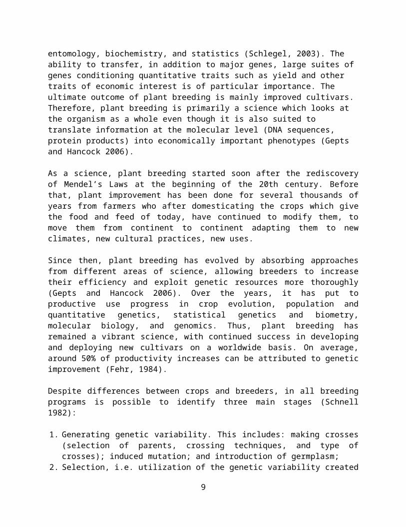
trials. An important characteristic of a breeding program is that is a cyclic process in which each step feeds information and material into the subsequent step, and each cycle feeds information into the next cycle (Fig. 1)1. During this process a tremendous amount of information is generated and a major challenge in a breeding program is how to capture and store this information in a way that is sufficiently transparent for others (scientists and non-professionals) to use. In CPB programs most of this information represents the ‘cumulative experience’ or the ‘knowledge of the germplasm’ that the breeder slowly accumulates over the years.

Figure 1. Schematic representation of a typical centralized- non participatory plant breeding program that for a large part takes place inside a research station (the first three stages which usually last more than 10 years) with all the decisions being taken by the breeder’s team.

Together with a definition of plant breeding is also important to define who is a plant breeder.

The traditional definition of a plant breeder includes only those scientists who have the full responsibility of a breeding program, made up of subsequent cycles as the one shown in Figure 1, to develop new cultivars and improved germplasm; however, many feel this definition should be expanded to include scientists who contribute to crop improvement through breeding research (Ramson et al. 2006). In this manual we will use the traditional definition of a plant breeder because we believe that only the scientists who have the full responsibility of a breeding program can implement PPB programs.

Participatory Plant Breeding (PPB)

A PPB program (Figure 2) is similar to a CPB program. In particular, it maintains the typical cyclic structure of a breeding program, with three important organizational differences: Most of the program takes place in farmers’ fields (decentralized);1Most breeding programs in Australia do not follow the scheme in Figure 1 as they are decentralized in farmers fields but with no involvement of the farmers’ in the selection process.

9

The decisions are taken jointly by the breeder and the farmers; The program, being decentralized, can be replicated in several locations

with different methodologies and type of germplasm (Fig. 3).The broken line in Figure 2 shows that the moment, usually in stage 2, when the breeding material is transferred in farmers’ fields is flexible, but it has to occur during this stage for the program to be defined as “participatory”. The later the transfer of the material to farmers fields occurs, the less participatory the program is because, as the breeding cycle progresses there is less and less breeding lines to choose from.Stage 3, which in CPB programs is partly conducted on-station and partly conducted on-farm, in the case of a PPB program is only conducted in farmers fields.

Being a highly decentralized process, participatory plant breeding is more flexible than conventional plant breeding both in terms of methodologies

than in terms of

germplasm.

Figure 2. Schematic representation of a decentralized - participatory plant breeding program: the stages which take place inside a research station are much less (the first and part of the second) with all the decisions being taken by the breeder’s team together with the farmers’ community. The broken line indicates the moment (which is flexible) when the program moves into farmers’ fields.

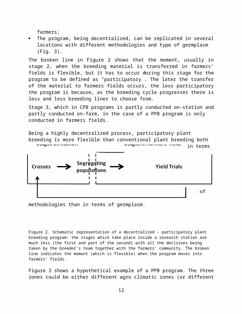
Figure 3 shows a hypothetical example of a PPB program. The three zones could be either different agro climatic zones (or different provinces or different states) within the same country or different countries. Within the zones farmers may grow the same crop for different uses, for example malting barley in one zone and feed barley in a different zone or improved wheat cultivars as cash crop and landraces for home consumption.

10

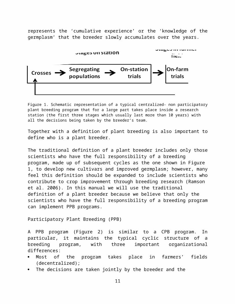
Figure 3. A decentralized - participatory plant breeding program can be replicated in various zones (= agro climatic areas or administrative provinces or regions within a country or countries). In each zone the program can use different crops, different breeding materials, and different experimental designs.

The knowledge of the type of germplasm needed by the farmers dictates the composition of the PPB trials that can differ from one zone to another.

Participatory Variety Selection (PVS)

Participatory Variety (or Varietal) Selection (PVS) is a process by which the field testing of finished or nearly finished varieties, usually ranging from 2-3 to 10-15, is done with the participation of farmers. Therefore, PVS is always an integral part of PPB but can also stands alone in an otherwise non-participatory breeding program if, using Fig. 1 as an example, farmers’ opinion is collected and used during the final stage, i.e. the on-farm trials.

Involvement of farmers during the last stage of an otherwise non-participatory breeding program has one major advantage and one major disadvantage: the advantage is that, if the farmers’ opinion becomes part of the release process which follows the on-farm trials, it will help proposing for release only the variety that farmers like, thus increasing enormously the speed and the rate of adoption; the major disadvantage is that because farmers’ opinion is sought at the very last stage of the breeding program there may be nothing left among the varieties tested in the on farm trials which meets farmers’ expectations. On the other hand, the disadvantage may induce the breeder to seek the farmers’ participation at an earlier stage

11

of the breeding program moving therefore from PVS to PPB.

PVS may also be used as a starting point, a sort of exploratory trial, to help farmers assessing properly the amount of commitment in land and time that a full fledge PPB program requires.

The Participatory Model of the ICARDA Barley Program

The model of PPB program that will be used throughout the manual is the model implemented by the PPB program used at ICARDA in barley, wheat, lentil and chickpea, i.e. self-pollinated crops which we believe can be applied also in cross pollinated and vegetatively propagated . The most important features of the ICARDA barley-breeding are the following:• After the initial crosses, done mostly to combine existing landraces or

improved or recommended but yet-to-be-adopted varieties and using, when possible the wild relatives, the crosses in the successive cycles are based on the lines selected by the farmers in the previous cycles of selection;

• The breeding method is the bulk-pedigree: F3 bulks are yield tested for four consecutive cropping seasons in the first (F3), second (F4), third (F5) and fourth stage (F6) yield trials;

• In those cases where varietal purity is required for the official release of the future varieties, the extraction of pure lines can be done on station as the bulks are promoted from one stage to the next, or at the end on the few superior bulks emerging from the fourth stage of yield testing;

• The decision on what to promote from one stage to the next is taken by the farmers in ad hoc meetings and is based on both farmers’ visual selection during the cropping season and on the data collected by the researchers or by the farmers after proper statistical analysis;

• In general researchers have primary responsibility for designing, planting and harvesting the trials, data collection and data analysis. Farmers are responsible for everything else and make all the management decisions. However, in some programs, farmers are also responsible for planting, harvesting and data collection.

• The statistical analysis is ‘state of the art’ using spatial analysis of unreplicated or partially replicated or fully replicated trials (Singh et al. 2003).

• In terms of the farmer’s time, the cost of participation ranges from two days to two weeks annually depending on the level of participation.

• A back-up set of all the materials tested in stages 1 to 4 is also planted at the research station to purify the bulks if pure lines are needed, but, more importantly, to produce the seed needed for the trials and to insure against the risk of losing the trials to drought or other climatic events.

12

• In some countries, the farmers who are hosting trials are compensated for the area used by the trials with an amount of seed equivalent to the production in a normal year.

• Seed cleaning machinery is supplied to some villages to assist in the multiplication and dissemination of selected varieties following the fourth year of farmer selection.

• Screening for diseases and insect pests is carried out on-station before the first stage of yield testing on farmers’ fields.

• The approach is flexible enough to accommodate biotechnological techniques, specifically Marker-Assisted Selection, after the first year of farmer selection. (PPB should be able to provide reliable information on desirable traits that could later be evaluated via Marker-Assisted Selection).

How to get started: organizational issues

As defined earlier, a PPB program is necessarily decentralized. Therefore, we will start by discussing the organizational issues involved in transforming a breeding program from centralized to decentralized. Transferring a breeding program to outside a research station almost always implies losing some degree of control of a number of steps and operations. This is often associated with the perception that less control by scientists is associated with less precision, and this explains the reluctance with which several plant breeders, particularly those in the developing countries, operate away from their research stations.

Within a research station, all the operations associated with running a breeding program are shared by staff belonging to the same institution and having daily interaction (which does not necessarily make things easier). When a number of stages are transferred outside the research station, a number of operations can, and actually should, be shared with staff belonging to other institutions or to out-posted staff of the same institution, or a combination of the two.

Depending on the presence or absence of a strong extension service, and of the structure of the research institute responsible for the plant breeding, a number of different scenarios are possible.

In the case of countries with a strong extension service and the presence of regional (or sub-regional or provincial) research centers with infrastructure such as offices, computer facilities, agricultural equipment (including plot machinery), a DPB program could be organized based on the following principles:

13

• The scientist(s) at the institute’s headquarters are responsible for the preparations of trials (choice of entries, plot size, experimental design, and having the seed in envelopes ready for planting), the preparation of field books (or electronic files for electronic capture of field data), the preparation of draft field maps with possible alternatives for the layout of the trials, and the shipment of trials with all the detailed instructions for planting and note taking.

• At the headquarters there will be a central database where all the information generated in the breeding program is kept. Information generated in the regional centers should also be kept where it was generated as a form of safety duplication.

• The main responsibility of the staff of the extension service is to collaborate in the selection of the sites and the specific fields, according to the type and objectives of trials and the general philosophy of the breeding program.

• The research staff in the regional centers is responsible for implementing the trials on the ground, ensuring the required management, the timing of the field operations and eventually for collecting field data, which are then transferred to headquarters for statistical analysis. Alternatively, when the necessary expertise is available, they can be requested to do the single site statistical analysis, leaving the responsibility for the multi-site statistical analysis to the headquarters.

• Extension and research staffs are also responsible for the organization of field days. These are useful not only to show the potential clients the new breeding material, but also to understand through the interaction with farmers whether the experimental setting (location, type of soil, type of management, etc.) is actually representative of farmers’ conditions.

This overall organization is facilitated by involving all staff participating in the implementation of the breeding program in regular meetings, through which the basic principles of the breeding program are understood and shared by everyone. This obviously includes the full sharing of results among all the participants on an annual basis.

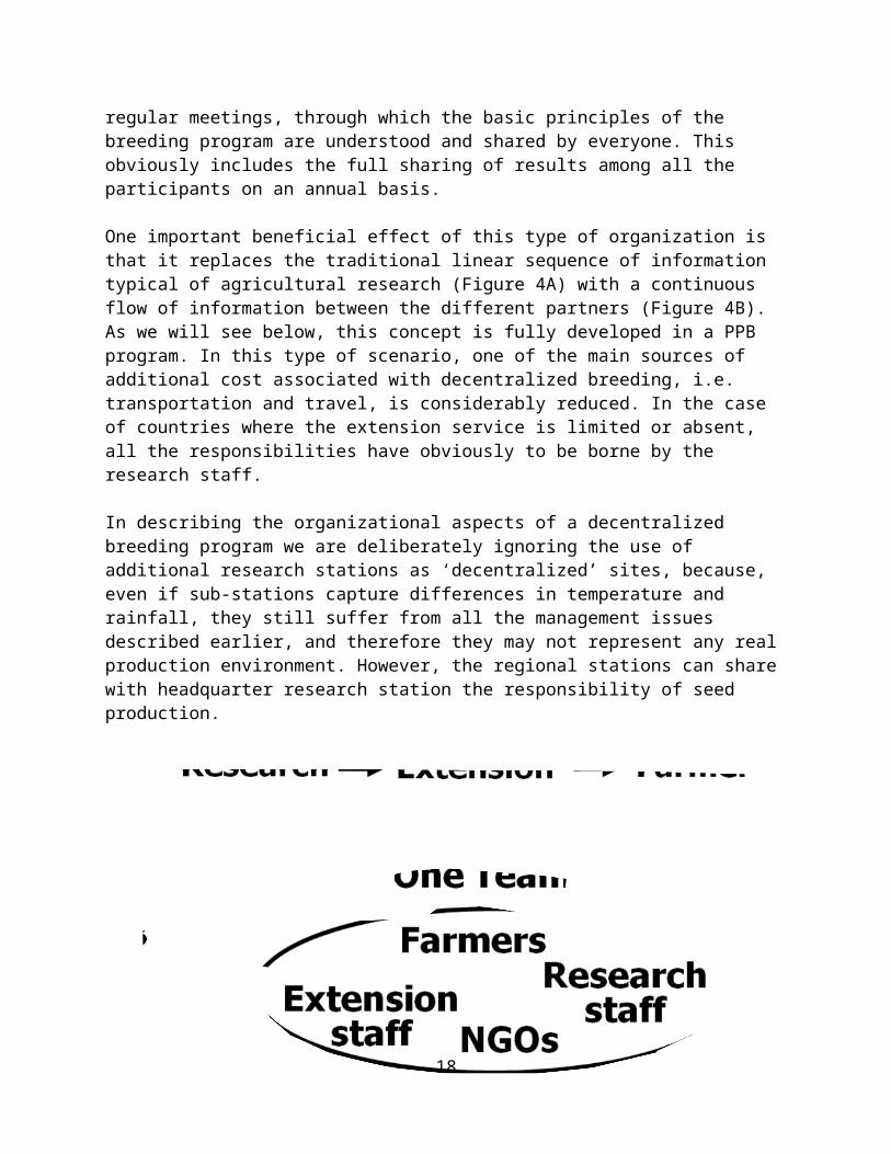
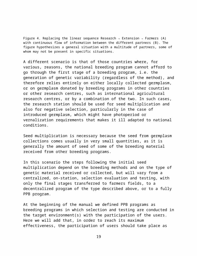
One important beneficial effect of this type of organization is that it replaces the traditional linear sequence of information typical of agricultural research (Figure 4A) with a continuous flow of information between the different partners (Figure 4B). As we will see below, this concept is fully developed in a PPB program. In this type of scenario, one of the main sources of additional cost associated with decentralized breeding, i.e. transportation and travel, is considerably reduced. In the case of countries where the extension service is limited or absent, all the responsibilities have obviously to be borne by the research staff.

In describing the organizational aspects of a decentralized breeding program we are deliberately ignoring the use of additional research stations as

14

‘decentralized’ sites, because, even if sub-stations capture differences in temperature and rainfall, they still suffer from all the management issues described earlier, and therefore they may not represent any real production environment. However, the regional stations can share with headquarter research station the responsibility of seed production.

Figure 4. Replacing the linear sequence Research → Extension → Farmers (A) with continuous flow of information between the different partners (B). The figure hypothesizes a general situation with a multitude of partners, some of whom may not be present in specific situations.

A different scenario is that of those countries where, for various, reasons, the national breeding program cannot afford to go through the first stage of a breeding program, i.e. the generation of genetic variability (regardless of the method), and therefore relies entirely on either locally collected germplasm, or on germplasm donated by breeding programs in other countries or other research centres, such as international agricultural research centres, or by a combination of the two. In such cases, the research station should be used for seed multiplication and also for negative selection, particularly in the case of introduced germplasm, which might have photoperiod or vernalization requirements that makes it ill adapted to national conditions.

Seed multiplication is necessary because the seed from germplasm collections comes usually in very small quantities, as it is generally the amount of seed of some of the breeding material received from other breeding programs.

In this scenario the steps following the initial seed multiplication depend on the breeding methods and on the type of genetic material received or collected, but will vary from a centralized, on-station, selection evaluation and testing, with only the final stages transferred to farmers fields, to a

15

decentralized program of the type described above, or to a fully PPB program.

At the beginning of the manual we defined PPB programs as breeding programs in which selection and testing are conducted in the target environment(s) with the participation of the users. Here we will add that, in order to reach its maximum effectiveness, the participation of users should take place as early as possible, and ideally at the beginning of stage two in a plant breeding program, as described in Figure 1.

The organizational aspects of a PPB program do not differ conceptually from those of a CPB program. The major difference is that the decisions and the choices for the organizational aspects involve all the stakeholders, and the type of participation depends on how, when and which stakeholders are involved.

We will examine the following organizational aspects:

• Setting criteria to identify target environments and target users;• Choice of users (different uses of the crop, gender, age wealth, etc.);• Choice of locations (representativeness, relevance for the crop, different

agro climatic environments);• Identification of the target environment and users;• Type of participation;• Choice of breeding method;

Naming of varieties;• Management of trials in farmers’ fields;• Choice of type of genetic material, field layout, machine vs hand

operations, data analysis, and multi-environment trials (MET);• Institutionalization of participatory plant breeding;• Managing the transition phase.

As mentioned earlier, some of these organizational aspects are common to all breeding programs, while some are specific to PPB.

Setting criteria to identify target environments and target users

A PPB program may lose a great deal of its potential effectiveness if the sample of both environments and users in which the program is implemented does not represent both the target environments and the target users. In order to do that, setting the criteria for identification of the target environments and users is a critically important step.

In setting the criteria, it is useful also to assign priorities to the different categories of environments and users so that, depending on the resources available to the program, environments and users can be added or

16

discontinued on the basis of priorities established in an ideal context.

The most obvious criterion for the choice of the target physical environments, is their representativeness of the major production areas for a given crop (or for the crops covered by the program) in terms of climatic conditions (temperature, rainfall, elevation), agronomic practices, soil types, landscape, etc. The criteria for the choice of the socio-economic environments are closely interconnected with those of the target users. Therefore the program has to decide whether to work for all the various socio-economic environments present in the target area, or to privilege the most difficult environments where farmers have fewer opportunities for market access and where most of the agricultural products are used within the farms or within the community, or to work only for the most favourable, high potential, environments. As mentioned earlier, PPB has evolved mainly to address the difficulties of poor farmers in developing countries (Ashby and Lilja 2004) which have been largely bypassed by the products of CPB. In fact there is no reason why the approach should be confined to work with low-income farmers. Basically, when done properly, PPB is an approach that, even if applied in a variety of modes, merges the technical knowledge of the ‘scientists’ with the knowledge of the ‘farmers’, which is historically based on millennia spent in domesticating wild plants and adapting the resulting crops to a multitude of different environments. Therefore, in principle, PPB can apply equally well even in situations of market-oriented agriculture in favourable environments. It seems particularly suited for organic agriculture.

The main criteria to identify farmers can be grouped in three broad categories:

• Farmer characteristics: these include language, ethnicity, caste, age, gender, income, education, market relations or orientation, membership of farmer organizations (unions or cooperatives), and relationships among groups within the same community and between communities.

• Farmer expertise: this includes the need to understand whether farmers are already practising some types of plant improvement, as this is essential in the choice of the breeding methodology (see below). In some communities, e.g. Eritrea, specific individuals have specific responsibilities in relation to crop and variety introduction (Soleri et al. 2002).

• Farmer needs These include the needs of different groups, their perception of risk and hence the type of variety they consider more appropriate in term of stability and yield (Soleri et al. 2002), and the need for special quality attributes either for feed or for food, or both. These include also the farmers’ understanding of production limitations with reference to the use of fertilizers, appropriate rotations and irrigation. It is also important to understand farmers’ needs in terms of seed supply, because it makes a large difference whether the farmer predominantly

17

use their own seed (or the seed of their neighbours), or usually buy seed from the formal sector.

Identification of the target environment and users

Once the criteria are set, the actual process of identification needs the involvement of partners who have a very good knowledge of both the environment and the users. These are typically the staff of the extension service or the staff of the outlying research stations. The first step is to set meetings with all the stakeholders with the objective of identifying partners and locations.

In this phase there are some potential biases that can affect the success of PPB. Key decisions affecting the participatory program are (i) whether to seek individual or group participation; (ii) whether the participants should be experts (germplasm experts are farmers who regularly experiment with varieties, are able to recognize important intra- as well as inter-varietal differences, and who target specific varieties to different micro-niches) or whether they should represent the wider community; and (iii) whether equity should be the main objective in the identification of the users. Meetings with all different typologies of farmers may be inappropriate without a proper knowledge of the power relationships within the community. This usually leads to a few farmers monopolizing all the discussions reducing the possibilities for others to express their views. This danger varies greatly with the culture: in some cultures, women are not even allowed to attend meetings; in others, they can participate with a passive role; and in others they can participate freely and with the same rights as the men. Therefore, it is not possible to give a ‘cookbook formula’ for what works better. In general, if some groups or individuals tend to be discriminated against, it may be appropriate to have separate meetings with different social, gender, age or wealth groups.

In the process of identifications of users, it is very important to clarify (i) what plant breeding can offer and how long it can take; (ii) what sort of commitment in land, time and labour is required from the farmer; (iii) what is the risk for the farmer and how this can be compensated for (in-kind compensation vs. money), and (iv) what the overall benefits are that the farmers can expect if everything goes well.

In these meetings it is also essential to understand what sources of seed farmers use for the various crops, to anticipate which type of change the participatory program might introduce, and to make sure that farmers are aware and prepared to absorb the changes.

The organizational issues of the choice of sites are both at the macro- (identification of villages or locations within a country or a region) and at the

18

micro-level (identification of the field within a village for planting the trial(s). The participation of farmers in the identification of the fields is unavoidable because it is associated with the relevance of the results and with the issues of ‘who participates’ and ‘who benefits’: it is at this point that small-scale farmers run the risk of being excluded as active participants because their land is not large enough to host trials in addition to the farmers’ crop. As we will see later, it is possible to find experimental designs that allow distributing relatively large number of entries in small blocks, each planted in a different farmers’ field. An additional organizational issue in the choice of the sites, which is associated with the issue of the breeding philosophy, is whether they should be sufficiently representative to allow some degree of extrapolation of the results to other sites, or whether the priority should be to meet farmers' needs to target micro-niches. In practice, it is advisable that sites do represent the range of environmental and agronomic conditions in which the crop is grown, because this is known to have a major effect on farmers’ selection (Ceccarelli et al. 2000; 2003).

PPB programs are often seen exclusively as programs leading to niche varieties, adapted to only a restricted complex of environmental and social characteristics. This is not necessarily true, as the type of adaptation (narrow or wide) of the varieties emerging from a PPB program is largely dependent upon the nature of the locations and the users. If the locations covered by the program represent a mix of favourable and unfavourable growing conditions, it may be expected that the more uniform environmental conditions that generally characterize favourable environments will led to the selection of the same varieties across a number of locations (widely adapted in a geographical sense), assuming that farmers’ preferences are also homogenous across the same locations. In the more unfavourable conditions, one can expect that more location-specific varieties (narrowly adapted) will be selected. Eventually, even if the selection is conducted independently in each of many locations, giving the impression that selection is for specific adaptation, the process will not discard a truly widely adapted genotype if such a genotype does exist in the breeding material (Ceccarelli 1989). Therefore a PPB program easily results in a mixture of widely and narrowly adapted varieties.

What is discussed above also depends on the definition of wide and narrow adaptation. Narrow and wide are relative terms; therefore, for an international breeding program, a widely adapted variety is a variety performing well in a number of countries, while for a national breeding program it is a variety performing well in several locations within the country, while, ultimately, to a farmers it means a variety performing well across cropping seasons – without too much concern whether it performs well elsewhere.

19

It is difficult to reach an optimal allocation of resources regarding to the number of sites and to the number of farmers at each site. As we will see later, it is possible to organize a PPB program in such a way that G×E interaction, and more specifically Genotype × Location (G×L) and Genotype × Years within Locations (G×Y(L)) will eventually optimize the overall structure, at least from a biological point of view.

Type of participation

Several scientists (Biggs and Farrington 1991; Pretty 1994; Lilja and Ashby 1999a, 1999b; Ashby and Lilja 2004; McGuire et al. 1999; Weltzien et al. 2000; 2003) discriminate among different types or modes of participation, which are not necessarily mutually exclusive, although there may be trade-offs among the impacts of the different types. We will not discuss these different typologies because field experience indicates that PPB is a continuously evolving process. It is quite common that, as farmers become progressively more empowered — an almost inevitable consequence of a truly PPB program — the type or mode of participation also evolves.

Choice of parental material

The choice of parental material is of critical importance in a breeding program. Here we only add that, as in a CPB, the parental material in a PPB program is, with few exceptions, the best material selected, by farmers in the previous cycle.

Choice of breeding method

The breeding method is only one of the factors determining the success of a breeding program; the others include the identification of objectives and the choice of suitable germplasm (Schnell 1982).

In CPB, the choice of the breeding method is purely the responsibility of the breeder and is largely affected by the breeder’s scientific background and by the mandate of the organization, public or private, for which the breeder works.

In PPB, the choice of the breeding methods cannot be made without considering whether and how farmers are handling genetic diversity. The rationale is as follows. As shown in Fig. 1, the generation of variability is the first step of any breeding program, conventional or participatory, followed by the utilization of variability and eventually the testing of the prospective varieties. In a number of countries, farmers do use genetic diversity either as a specialized activity within the community, or as an individual initiative. For example, in Eritrea it is common for farmers to select individual heads within a wheat or a barley plot, plant them as head rows in a small portion of their

20

field, decide whether to bulk one or more rows and start testing the bulk in the field of other farmers, initially on a small scale and gradually on a larger area. One of the most widely grown wheat varieties in the country has been developed starting from a small seed sample bought by an expert farmer in a local seed market and planted initially as spaced plants. In Nepal, before harvesting the crop, a woman farmer growing an old barley landraces habitually collects a sample of heads representing all the different morphological types present in the field to produce the seed to be planted in the following cropping season. In the northernmost part of India (Sikkim) farmers maintain and improve their rice varieties, by carefully selecting (before harvesting) the best panicles, which are then stored for the next planting season, while the rest of the crop is consumed. In contrast, in Syria and in many other countries in the Near East and North Africa, the selection unit is a plot, and excessive heterogeneity within a plot not only is not exploited, but is also considered undesirable.

These examples indicate that, even within the same crop, a PPB program has to use different breeding methods, at least at the beginning of the program, to ensure full participation. It is obvious that a blanket approach, based on the same breeding method used everywhere regardless of whether and which skills farmers have in handling genetic variation, cannot ensure true participation, as farmers will be confronted with methodologies they cannot relate to anything with which they are familiar.

In addition to the examples given earlier, breeding methods may differ for the same crop within the same country. Using Africa as an example, barley is grown in Ethiopia and Eritrea both as food and feed (largely landraces) and also for malt production for local breweries. While population methods can well be used in the first case, pedigree breeding or single seed descent (SSD) is more suitable in the second.

An issue related with the choice of the breeding method is how much breeding material farmers can handle. This is a controversial issue, and several scientists believe that farmers can only handle a very limited number of genotypes and therefore, implicitly, believe that the only form of participation is PVS. If true, this will make it impossible to implement true PPB programs, because plant breeding needs to start from a sufficiently large sample of genetically variable material.

Field experience shows that when discussing the number of genotypes farmers can handle, it is very dangerous to make assumptions before discussing the issue with them.

The choice of the breeding method also depends of the genetic structure of the final product, i.e. pure lines, mixtures, hybrids or open pollinated varieties. It is important to note that farmers can change the type of final

21

product originally planned by the breeder. For example, in Syria, where, in the case of self pollinated crops, the formal system only accepts pure lines for release, farmers do not mind adopting bulks as long as they are not too heterogeneous. In the case of barley, we also have the example of one farmer testing the advantage of a mixture of a 6-row genotype, adapted to high rainfall and lodging resistant, with a 2-row genotype adapted to low rainfall and lodging susceptible. Similarly in Egypt, we found that farmers plant a mixture of all the lines selected one year earlier (Grando, pers. comm.).

In principle, all breeding methods used in CPB can be employed in PPB, keeping in mind that ‘participatory’ does not mean that ALL the breeding material has ALWAYS to be planted in farmers’ fields.

Several examples of different breeding methods used in actual participatory breeding programs can be found in Almekinders and Hardon (2006).

Given that plant breeding is a cyclic process, one organizational issue that is often debated is the stage of the plant breeding program at which participation should start. As mentioned earlier, this issue in effect makes the difference between PPB and PVS, where the participation of farmers takes place during the third stage of the breeding process, after the genetic variability available at the beginning of the cycle has been — usually — drastically reduced. We believe that farmer participation should, at a minimum, coincide with the second stage of a breeding program, possibly when the genetic variability is still at or near its maximum. There are examples of PPB programs where farmers can start as early as making crosses, such as the participatory rice breeding programs in Bhutan, the Philippines and Viet Nam (SEARICE, 2003), which does not necessarily imply only emasculation and manual pollination, but, for example, mixing different genotypes or cultivars of cross-pollinated crops to facilitate inter crossing. A similar example is the improvement of maize landraces coordinated by the Centre for Chinese Agricultural Policy (CCAP), a leading agricultural policy research institution part of the Chinese Academy of Sciences (CAS). Even when farmers do not manually make the crosses, in a PPB program that runs over cycles of selection and recombination like any other plant breeding program, farmers control the crossing program by selecting the best entries, which are usually the parents of the following cycle, as discussed earlier under choice of parental material.

Eventually, a breeder planning to start a PPB program is faced with the issue of whether the breeding method used in a non-participatory program needs to be changed. While there are breeding methods that are easier to fit into a participatory context, a breeder does not have necessarily to change the breeding method, given what was said earlier about fitting the method to whatever type of breeding farmers are already doing. Here, we might add

22

that, like other aspects of PPB, the methodology can also evolve as new farmer skills emerge. Several examples can be found in Almekinders and Hardon (2006).

Naming of varieties

At the end of each cycle of the program, the four stages of yield testing mentioned earlier (see pg. 11), and if the cycle has been successful in producing a potential new variety that the community of farmers have contributed to select, one issue is how to identify the variety given that the numbers or pedigrees used by the breeders can meaningless to the farmers. In mature PPB programs it is now a consolidated habit to name those lines that farmers decide to plant on large areas after the 4th stage of yield trials. In mature programs this rarely results in conflict and the names chosen range from the name of village, the name of the son or daughter of a lead farmer, or symbolic names as peace, unity etc.

In relatively young programs we found, surprisingly, that the choice of the name may also be a moment of conflict the first time it occurs and that therefore it may be wise to raise the issue some time before or even at the beginning of the program.

Management of trials in farmers’ fields

The organizational issues of implementing trials in farmers’ fields differ considerably from those in a research station.

The first differences are issues such the choice of the actual portion of land on which to plant the trial, the total number of plots in each trial, the type of controls (check varieties), the plot size, the seed rate, the distance between rows, the dates of planting and harvesting, the importance of border (guard) rows and plots: all these have to be discussed with each community in each location. It is not simply a matter of courtesy. Farmers’ interest in the trial is directly proportional to their participation in its design and management. The inability of the scientists to accommodate farmers’ requirements may lead to a total lack of interest by the farmers. For example, in the case of barley in Syria, farmers believe that seed rate is extremely important. Whether this belief is correct or not is immaterial, because if the scientists use the seed rate they believe right, farmers may even refuse to carry out selection. Therefore, in the PPB program in Syria for example, we are using as many as eight different seed rates, ranging from 100 kg/ha to 250 kg/ha. As this is believed by the farmers to have a major effect on barley yields, an important side-activity would be to organize visits by farmers to locations where a different seed rate is used; this might be the best way to generate an interest in testing alternative seed rates.

23

One fundamental principle in discussing organizational issues with farmers’ communities is to pose and justify the problem, not to present a solution. The solution should come from the community, and if the community or the individual farmers are not prepared to solve the problem, a possible solution can be offered, but only as a suggestion.

The choice of land, which in a conventional breeding program usually depends on the farm manager, in the case of PPB has to be agreed on by the farmer. It has to represent a suitable rotation and a good uniformity (this should be checked the year before, together with the past history of the field). The size required by the trial may be smaller than that allocated by the farmer to that specific rotation. In this case, the extra land has to be planted by the scientists with a cover crop using a variety of the same crop chosen by the farmer.

The type of genetic material to be used in the program needs to be discussed with farmers. Initially, the scientists may find that farmers are not aware of the diversity within the crop, and in this case our suggestion is to start with a wide array of genotypes representing as wide range of diversity as possible. But there are cases where farmers have previous experience with various type of germplasm and they may feel very strongly concerning one or more types of specific germplasm type. For example, in Syria, farmers grow two landraces: one with black seed, which is grown predominantly in dry areas, and one with white seed, which is grown predominantly in wetter areas. Farmers feel very strongly about the seed colour and therefore in the participatory barley breeding program in Syria we make available different initial genetic material in the two areas. The issue of the type of genetic material covers also the issue of the checks. As we will see later in the section on Experimental designs, the checks have the dual purpose of providing an estimate of error variance (for example, in unreplicated trials with systematic checks) and to provide a comparison for farmers during selection. The ideal solution is to have a well adapted variety to fit both purposes, and if the choice of the check(s) is left, as it should be, to the farmers, this is usually their choice.

Managing the equipment in a PPB program can be a challenging issue. If the country has a network of research stations each with its own equipment, it is obviously more economical that each station uses its own equipment for all the field operations. Where machinery has to be moved from one central research station to all the trials sites, the number of sites and of trials has to be adjusted to allow all the necessary operations to be performed in time. Usually farmers are extremely concerned about planting and harvesting at the right time, and if the choice is between having several locations and being late in both planting and harvesting some of them, it is advisable to reduce them to a number that can be managed properly. The issue of timely harvesting, in the case of completely mechanized crops, can be solved by

24

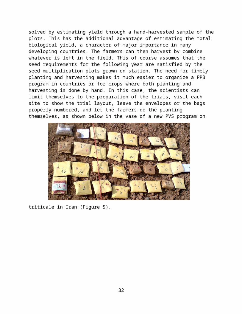
estimating yield through a hand-harvested sample of the plots. This has the additional advantage of estimating the total biological yield, a character of major importance in many developing countries. The farmers can then harvest by combine whatever is left in the field. This of course assumes that the seed requirements for the following year are satisfied by the seed multiplication plots grown on station. The need for timely planting and harvesting makes it much easier to organize a PPB program in countries or for crops where both planting and harvesting is done by hand. In this case, the scientists can limit themselves to the preparation of the trials, visit each site to show the trial layout, leave the envelopes or the bags properly numbered, and let the farmers do the planting themselves, as shown below in the vase of a new PVS

program on triticale in Iran (Figure 5).

Figure 5. Paper bags representing one replication of a PVS trial in triticale laid down in the field ready to be hand planted by the farmer.

The issue of managing the equipment in a situation of fully mechanized operations can also be addresses by empowering farmers to conduct trials. This often poses technical challenges, because commercial drills and

25

combines are not suitable for planting experimental plots.

Finally, two additional issues in managing trials in farmers fields concern the physical layout of the trials, and the management of crop residues, border rows and leftovers (in the case of sampling).

In arranging the trials on the ground, three principles are important: the first is that no land should be left uncultivated. In many farming communities in developing countries, leaving even a few square metres of land uncultivated is considered almost a crime, and this is particularly true in marginal and dry areas where yield per unit of land is low. Therefore, no gaps should be left between plots, as is common practice on research stations to facilitate the identification of plots, and the alleys should also be planted. To facilitate farmers during selection, and to avoid seed mixture if the seed from the trial is to be used the following year, the first and last rows of the plot can be harvested by hand shortly before selection and harvesting. Similarly, the alleys can be mechanically slashed or hand harvested to facilitate moving across the field and harvesting. The second principle is to lay out the trial in a fashion that it occupies a piece of land of regular shape, because this facilitates the handling of the rest of the land by the farmer. The third is that the trial should be always surrounded by border plots which assure that all the entries are tested in same condition of competition, that there is a buffer protecting the tested entries from possible damage, and may be offer the opportunity to multiply the seed of a variety needed by the farmers.

The management of trials residues (borders, fillers around trials, border rows and what is left of a plot after taking samples) is an important organizational issue because it is a potential source of dispute. As a general principle, as in many other organizational issues in PPB, this needs to be discussed in advance with farmers, justifying why the handling of experimental plots is different from the handling of a field planted for large-scale production, underlining the need to generate information to use later in selection, and the need for as much precision and accuracy as possible to obtain correct estimates of the genotypic values of the breeding material (the scientists do not necessarily have to use these terms when discussing with farmers!). As mentioned earlier, the guiding principle is to justify and pose the problem, and involve farmers in the process of finding the most mutually suitable solution.

Farmer selection

A key organizational issue in PPB is the selection done by the farmers. This is one of the most important operations (and one that makes the breeding program participatory). It is also one of the activities that, if done properly, can generate a strong sense of ownership, and enhance farmer skills as far as the knowledge of the genetic material is concerned.

26

As for other organizational issues, it is impossible to give general recommendations, because the baseline can be very different in different communities. One of the extreme situations is represented by communities where there is only a vague notion that different varieties do exist, but farmers have had only sporadic contacts with scientists, and these contacts have been mostly of the type “I am here to tell you what do; you do it, and I will come back to check if you did it well!”. In these communities, farmers often ignore the sexual reproduction in plants and therefore the diversity itself within a crop is surrounded by an aura of mystery. The other extreme is represented by communities who already have a solid experience in breeding and experimenting.Most of our experience has been with the first type of situation, which is not necessarily the most difficult, but is certainly the one in which PPB takes more time to develop. Therefore we will illustrate some general principles that we followed with the first type of situation, and how these principles need to be modified in the case of the second situation. We will consider in particular two aspects of farmers selection, namely ‘when to select’ and ‘how to select’.

The timing of selection depends strongly on the crop and its uses, on the environment and on the traits farmers consider important. This is a typical aspect of the overall activity, and one which needs to be discussed with farmers during the planning of the program because it has implications on the amount of time farmers need to allocate to selection and on the total number of experimental units (plots or plants) farmers can handle. It also has implications for the degree of involvement of the scientists where some of the traits that are important to the farmers need to be measured.

The choice of the ideal time for selection is highly individual: some farmers prefer to visit the field often during the cropping season, while others, particularly in unpredictable environments, claim that only shortly before harvesting is it possible to assess the real value of the breeding material. Farmers may also change their preferences in relation to both when and how to select. Farmers who were used to an organized ‘selection day’, whereby all the farmers assembled at a meeting point and visited and scored the various trials, subsequently demanded to do the selection by themselves on a date convenient to them. In fact, it is obvious that while the first way of organizing the selection favours exchange of ideas among the participants, it also implies fixing a date in advance that later may be no longer convenient to some participants. The second solution has the advantage of allowing many more farmers to do the selection as they are free to choose when to do it. This obviously requires that the scoring sheets be made available ahead of time.

The scoring method using by farmers during selection is another

27

organizational issue, and like many others, the starting point can be different in different countries and in different communities within the same country. In some communities, some farmers are used to score different entities based on merit or value; in others there is no previous experience. The example of scoring the school homework of students is often useful. For some farmers, it is easier to use words representing different categories such as ‘undesirable’, ‘acceptable’, ‘good’, ‘very good’ and ‘excellent’, which later be translated into a numerical scale. With time, and particularly with those farmers participating regularly in the selection session(s), the scoring method may change, particularly when farmers within the same community use different methods and farmers will eventually converge towards a common scoring method.

When scoring implies ‘writing’ (words, symbols or numbers) there is risk of excluding farmers unable to read or write. The problem can be solved by flanking the farmers who need assistance with a researcher, an extension staff member or another farmer; this requires additional organizational arrangements, particularly in remote areas. In those cases, the ideal solution is to make the communities capable of organizing themselves as much as possible.

Other methods of scoring breeding material include the identifications of the best entries with ribbons of different colours (depending on the category).

This issue will be discussed further in the section on data collection.

Visits to farmers

In a PPB program it is very important to maintain contacts with farmers beyond and besides specific scientific activities. These ‘courtesy‘ visits are not only instrumental in building and maintain good human relationships between scientists and farmers by bridging gaps, but are an incredibly fertile reciprocal source of information. Often farmers like to converse on issues not directly related with the specific participatory program, but related to the multitude of challenges that farmers, particularly those in marginal agricultural environments, continually face. This helps scientists to put the issue of developing new varieties of a given crop in a broader context.

Managing the transition phase

In this section we will consider the organizational issues faced by breeders who decide to migrate from a CPB to a PPB program. We will not consider the case of transforming decentralized non-participatory breeding programs, such as most of the Australian breeding programs, into participatory programs because this only require solving the organizational issues associated with farmer participation discussed above.

28

In general, the problem is to transfer a cyclic process taking place largely within one or more research stations to farmers' fields, and to change the process of decision-making in the way discussed earlier. The general organizational issues in managing the change is that, because it is unwise to get rid of breeding material, the transfer of the program to farmers' fields should start from the first step that the breeder intends to transfer and implies that, till the transfer is completed, the CPB and the PPB program will coexist.

Sharing and Dissemination of Findings

Once the results of the PPB trials for each location have been compiled, they should be shared with all the stakeholders (other farming communities, NGOs, and Extension). This can be done through a combination of methods including:

Organizing a field day at which participating farmers explain and present their work and results

Documenting the work using radio and television Holding stakeholder meetings to share the results Training participating farmer groups Producing descriptive sheets for each farmer’s selected variety.

Data Collection

The trials conducted in a PPB program need to generate the same quantity of information and of the same quality as those in a CPB program, for two reasons: first, because the information has to be used to decide which material to promote and which material to discard ̶ the scientists have a moral obligation to provide farmers with most precise data ̶ , and, second, because the information can be later used when submitting a variety for release. We learned that in addition to the visual selection, farmers may want to have access to some quantitative data to reach a final decision. This is an additional issue to discuss at the onset of the program because if this is required by the farmers, the trials have to be organized in such a way as to allow collecting data on the traits considered important by farmers, analysing the results with appropriate statistical analysis, and reporting the results in a format that makes the information fully accessible to farmers.

Collecting field data may go beyond the time, the facilities and the expertise of the farmers, but this is a possibility that cannot be ruled out a priori. However, as in most similar cases, the issue needs to be discussed with the farmers so that it is becoming almost a service that the scientists provide them.

29

The traditional manner of organizing data capturing is the manual recording through field books. Field books can be produced using specialized software tools, such as AGROBASE™ (www.agronomix.mb.ca), Excel™ or databases such as Access™. Manual capturing of data has a number of disadvantages, including: the preparation of field books is time consuming; note taking is weather dependent (field books are very difficult to use on

windy or wet days); the data are handled twice, being written in the field book first and

entered in the computer later, thus increasing the probability of manual errors; and

the time required for data entry delays statistical analysis, usually until after harvesting, hence reducing the possibility of detecting errors by examining the results of an analysis conducted immediately after the data are collected.

Today data capturing can be easily done electronically using palmtops (there are very many types available on the market) or specifically designed devices, which are usually much more expensive. The file, which will normally be printed as a field book when data capture is by hand, is downloaded into the main memory or in the flash card (recommended) of a palmtop (they usually handle a variety of file types, depending on the brand), which can then be taken to the field to enter data. Electronic data capture has a number of advantages: data are entered manually only once and then transferred electronically to

the main computer for analysis; before leaving the field, it is possible to quickly check the data through

sorting and ranking, and immediately correct typing mistakes; data can be collected in the field under a wider range of climatic

conditions than with field books; data analysis can immediately follow data collection, thus providing an

additional means of checking for errors in data entry while the crop is still in the field; and

use of memory cards enables one to keep at hand in the field all the relevant information concerning all trials and nurseries in a large breeding programme.

At the end of the season it is always possible to produce a printout of all the files and to maintain a hard copy of all the data.

The list below is very indicative as it varies with the crop. In principle, all the data which are usually collected in a breeding program can be collected in a PPB program except perhaps those collected under controlled conditions.

30

Before Harvesting

Vigor (score (1 = poor vigor, 5= good vigor)Habit (erect vs prostrate with a visual score usually 1 = erect, 5 = prostrate)Plant height per plot (more measures per plot in case of segregating populations)Farmers’ score (example 0= bad, 4= very good). Can be an overall score or an individual score for each trait of importanceBreeder’s score (better if the same scale as the farmers’ score)LodgingDiseaseCold damageWilting

At Harvest

Grain yieldBiomassHarvest IndexAfter Harvest Seed SizeSeed color (when relevant)Quality traits (depend on the crop)

Derived data

Derived data are those that are not collected directly in the field but are derived from those collected. Typically, harvest index (grain yield/total biomass) is a derived data. Others could be spike length in cereals like wheat or barley which is usually measured by difference between the distance from ground level to the top of the spike excluding the awns and the distance between ground level and the bottom of the spike, or grain yield in kg/ha obtained by converting grain yield usually recorded in g/plot.

In addition to the average farmers’ score and the average breeders’ score (in the case more than one plant breeder scores the plot), three useful derived data in PPB trials are the percentages of farmers for which a genotype ranked in the top third, middle third and lowest third. These are called the TOP, MID and LOW values, respectively and a genotype that occurred mostly in the top third (high TOP value) is considered as a genotype preferred by the majority of the farmers. The derivation of these three values from the original farmers’ score can be obtained easily with the function "IF" of Excel.

The data which are peculiar of a PPB program are the farmers’ scores. There

31

are different ways of recording the opinion of the farmers.

One example of the simplest way for farmers to record their appreciation of a variety from a general point of view is by the number of thick marks or stars given to each plot as shown in Figure 6.

It will be noticed that the evaluation form does not contain the names of the varieties or breeding lines to avoid any bias. However, it is recommended that one or more scientists or technical staff present during the field selection should be able to provide this information in the case it is requested.

Figure 6. An example of a field book (in Arabic) filled by a farmer using thick marks (the more are the thick marks, the better is the plot, according to the farmer opinion). The thick marks can be replaced by numbers as shown in plots 111 and 118 and then analyzed statistically.

In other cases farmers’ prefer to score separately traits they consider important such as plant height, spike length, crop density, tillering and lodging (Figure 7). The specific traits which are scored obviously change with the crop and with the country. Within the same crop and the same country

32

they can also change with the use of the crop.

The analysis of data such as those shown in Figure 7 can be done either on the scores of individual traits or on the average score across traits.

Figure 7. Another example of a field book (in Farsi) filled by a farmer using a numerical scoring from 0 to 9 (0 = undesirable and 9 = very good) given to a standard set of five traits.

Figure 7 shows also the header that the score sheet for farmers’ scores should always have and that should contain the information below:

Name of farmer……………………………... Name of recorder (if different from the farmer). Village..........................................……Sub county/District.……………………………… Crop stage………….................……………Date …………………………………………………..Type of trial……………………………………..Plot number…………………………………………

33

Two methods by which farmers can evaluate varieties in a PVS program are the Pair wise ranking method and the Matrix ranking methods. The Pair wise ranking method consists in ranking of varieties or ranking according to attributes which can be done using a simple tabulation as shown in Table 1.

Table 1. Pair wise ranking method applied to 5 varieties. Variety A B C D E Total score Rank A x B C A A 2 3 B x C B B 3 2 C x C C 4 1 D x E 0 5 E x 1 4 Total 10

To evaluate the above example, compare the variety in the x column to the variety in the y column- for example variety B is preferred to variety A, variety C is preferred to all other varieties, while D is the least preferred. Ranking of varieties can be according to the different attributes e. g. resistance to pests and diseases, maturity, seed size, plant height and yield. The Matrix ranking methods can be very useful, especially in situations where many farmers cannot be brought together simultaneously to do the evaluation. Assume, for example, that there are 20 farmers carrying out on farm evaluation of four varieties (A, B, C & D) in a particular location (Table 2). The pair wise ranking methods done by individual farmers can be compiled into a matrix to give the overall ranking by the participants. Table 2. Example of varietal ranking by a group of farmers; the number of farmers ranking the varieties 1st, 2nd etc and overall ranking

VarietyIndividual rank

Rank index Overall rank1 2 3 4

A 4 1 10 5 56 3 B 10 3 6 2 38 1 C 3 14 1 2 42 2 D 3 2 3 12 64 4

Rank index= Summations of rank x number i.e., for variety A Rank index= (4x1) + (1x2) + (10x3) + (5x4) = 4+2+30+20 = 56. The lower the rank index, the more desirable is the variety.

Experimental designs for PPB trials

Table 3 shows some experimental designs which can be used for the various

34

stages of a participatory program. The choice of the designs is dictated by 1) the amount of seed available in the various stages, 2) by the average farm size in the target area, and 3) by the need to find a compromise between offering to farmers as many choices as possible while keeping the total number of plots to a manageable size.

Stage 1 trialsThe first stage of PPB is usually represented by trials composed by the same set of entries planted in as many locations as possible. In some cases, where there are strong differences in farmers’ preferences in different areas of the same country, it is advisable to prepare different trials with different type of germplasm. In both cases the trials should have a different randomization in each location.

Table 3. Experimental designs in PPB trials.Type of trial Experimental design

Stage 1(several entries, little seed per entry)

Un replicated with systematic checks or partially replicated in rows and columns or incomplete blocks in two replications in rows and columns

Stage 2 (less entries, more seed per entry)

Incomplete blocks in two replications in rows and columns

Stage 3 (few entries, much more seed per entry)

Incomplete blocks in two replications in rows and columns

Stage 4 (2-4 entries, large amount of seed per entry)

RCBD with farmers as replications

In stage 1 when the total number of new entries tested vary (in our cases) between as little as 50 to as much as 160, a compromise must be sought between the plot size and the number of locations. This compromise is reached by sacrificing replications in favor of locations as done in the majority of the CPB in their initial stages; these trials can be grown using from one to four checks repeated a sufficient number of times to have at least 30 degrees of freedom for the estimate of the error variance. Examples are trials with 167 entries and 2 checks repeated 16 and 17 times, respectively, or trials with 165 entries and 3 checks repeated 11, 12 and 12 times respectively. In both cases the resulting 200 plots are arranged in a rectangular grid of rows and columns with the possible arrangements (4 rows x 50 columns, 8 rows and 25 columns, and 20 rows and 10 columns) shown in Figure 8. The various arrangements allow a certain degree of flexibility in adapting the trial to various field shapes. Figure 8 does not show the border plots which should surround the entire trials no matter what the layout is.

In this type of trial the choice of the checks is important because they must represent a reference for the farmers during the selection process, they must

35

provide an unbiased estimate of the experimental error and, in the long term, they can be used to estimate response to selection. Therefore, when they are chosen, one has to consider that by changing them later in the course of the program implies a loss of information. Usually, farmers will insist that the local landrace(s) be included as check(s). Eventually improved

varieties, if adopted by some farmers, can also be added.

Figure 8. Three possible layouts of an unreplicated design with systematic checks and 200 plots.

The design shown in Figure 8 can be improved by replicating only part of the entries and not all as in a typical RCBD. For example, if in stage 1 it is decided to test 160 entries one can plant twice the 40 entries with more seed available (Fig. 9). The entries which are replicated twice do not need to be the same in every village. Ideally the replicated entries should be present in as many columns and rows as possible and will provide an estimate of the

36

error variance. The improvement is associated with the fact that in this case the error is estimated using a wider range of genotypes as compared with the few in the previous case. One additional advantage of the partially replicated design is a more efficient use of the seed resources. In fact it is quite common in the first stages of a breeding program to have different amount of seed for the different entries. Since the entry with the smallest amount of seed dictates the plot size and the number of locations, only part of the seed of all the other entries will be needed and as consequence a large amount of seed goes wasted.

Figure 9. One possible layouts of a partially replicated design: the plots with the replicated entries are the red squares. The other two possible layouts are as shown in Figure 8.

There could be cases where none of the layouts shown in Figures 8 and 9 fit the size of the farm where the trial should be planted. This is often the case of communities where each individual farmer has a very small farm. The danger in those conditions is to single out as participants those few farmers with enough land to host the trial. This is not necessarily bad if the farm size is the only difference between large and small farmers. However, usually large farmers are also using agronomic practices too expensive for small

37

farmers or not suitable to small fields and therefore their fields do not represent the majority of farmers in the community.

One solution is to layout the trial on an area

which covers

more than one farmer’s fields, an example of which is shown in Figure 10, where one of the 3 arrangements shown in Figure 8 or the trial shown in Fig 9 is planted on an area which embraces three different farmers’ fields.

Figure 10. The example of a large 1st stage PPB trial which is too large to be hosted by an individual farmer but that can be planted on a homogeneous piece of land spreading over different farmers’ field.

If the solution shown in Figure 10 is not feasible because, for example, farmers’ fields are separated by physical obstacles such as trees or channels or walls, or are at different levels like in terraces-type of agriculture, then it is still possible to use a relatively large 1st stage trial by using a replicated incomplete block design an example of which is shown in Figure 11.

The advantage of an incomplete block design is that each incomplete bloc (a

38

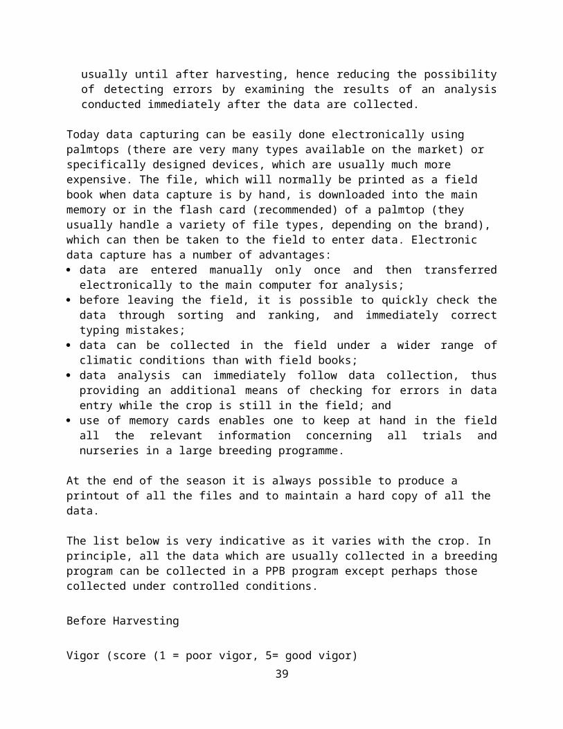
sequence of 20 plots in the example shown in Figure 11) is an independent unit and therefore can be allocated to a different field from each of the other incomplete blocks. The number of incomplete blocks which can be planted on each farm depends only on the farm size and therefore there can be fields with 3, 1, 2, 5 incomplete blocks. It is also possible that one full replication is planted by a large farmer and the 10 incomplete blocks of the other replication with 10 different farmers. The disadvantages of this layout are 1) the restriction that the total number of entries must be …………….. and therefore there are certain number of entries for which the design is not available and 2) the loss of the row and column design which, as we will see later, allows a spatial analysis.

REPLICATION 176 125 14 44 155 145 17 152 96 162 107 172 43 95 77 13 53 190 83 2531 106 66 119 1 61 139 108 33 174 198 193 97 65 149 143 51 12 148 18335 134 39 42 104 181 27 3 116 170 18 54 197 50 62 6 101 8 121 82177 58 88 79 94 41 24 30 136 192 56 86 117 52 4 168 142 122 68 60196 23 40 103 85 105 98 70 137 144 22 87 169 81 163 157 129 90 72 179165 123 114 89 91 47 9 195 7 146 161 16 126 92 29 76 64 153 21 7899 167 159 74 46 38 185 80 164 189 124 178 67 55 150 166 180 133 73 63115 19 128 184 69 75 59 100 160 141 37 28 32 173 113 200 93 130 49 84 132 187 120 20 5 194 191 131 147 11 127 138 111 199 10 45 154 135 175 26 158 36 109 118 57 2 102 186 171 15 34 151 110 71 156 188 140 112 182 48

REPLICATION 2146 102 23 147 103 3 95 18 49 153 14 185 117 33 60 48 124 174 127 19133 142 59 184 9 34 42 77 106 105 79 179 15 78 80 191 65 96 104 11192 115 107 63 84 101 110 5 167 145 154 36 161 27 149 157 72 52 58 97

39

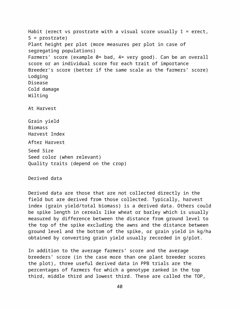
199 119 144 2 75 134 66 129 123 43 176 164 180 121 177 91 194 122 71 100150 170 56 7 166 25 116 61 141 187 1 109 171 20 37 21 163 70 192 5354 11 136 156 74 200 159 69 81 140 172 193 44 6 10 98 143 47 68 6490 28 8 131 38 51 30 169 130 83 94 76 45 155 29 108 118 181 188 67112 39 120 126 173 31 137 87 12 17 82 86 189 165 4 178 128 13 151 132195 114 186 160 148 50 99 26 85 32 73 175 197 125 57 183 162 168 88 19693 198 152 55 182 22 135 41 46 40 139 113 62 24 89 35 158 190 138 16Figure 11. An example of an incomplete block design randomized for 200 entries, 2 replications and incomplete blocks of size = 20 plots. One incomplete block is a sequence of 20 adjacent plots (like the sequence highlighted in yellow). The numbers indicate the entry number and their position the plot number: entry 76 is in plot 1 rep 1, entry 125 is in plot 2 rep 1, entry 25 is in plot 20, entry 31 is in plot 21, entry 146 is plot 1 rep 2 or plot 201 if a unique plot number is used.

Stage 2 and 3 trials

In the second and third stage of the PPB program, like in CPB, the number of lines progressively decreases as result of the farmers’ selection, while the amount of seed available for each entry increases. Another characteristic of the second and third stage of trials is that they usually contain different entries in each of the different locations in which the PPB program is conducted and in which the first stage trials were planted. This is a consequence of the selection being conducted independently at each location which usually results in different 1st stage entries being selected in different locations. Another difference is that, while there is usually only one 1st stage trials in each location, we suggest to have at least three 2nd, 3rd, and 4th stage trials at each location (Figure 12) This allows capturing differences within each location between agronomic practices, soil physical characteristics, uses of the crops, etc. and, as we will see later, conduct a genotype x farmer interaction analysis.

Because in these stages seed is less limiting than in the first stages we suggest using progressively larger plot size to be in the position of having a large seed supply of the lines which will be eventually selected.

40

Figure 12. A model of PPB program in which one farmer (the host farmer) in each village is hosting the stage 1 trials usually, but not necessarily, with the same type of germplasm but with a different randomization. After independent selection in each village, the selected entries (usually different, at least in part, from village to village) are planted in stage 2 trials by more than one farmer in each village and with a different randomization in each farmer. This is repeated in stages 3 and 4.

The experimental design to use is the replicated incomplete block design described at pg 31. As the number of entries in Stage 2 and even more so in Stage 3 is not very high (maximum 20-25 in stage 2 and 10-15 in stage 3) it is usually not necessary to subdivide replications and/or incomplete blocks in different farmers’ fields which allows maintaining the advantage of conducting spatial analysis.

41

Figure 13. An example of a stage 2 (or stage 3) replicated (2 replications) trial with 10 entries arranged in an incomplete block (block size = 5 – each block is represented by a different color) with two layouts: 2 rows (each row = 1 replication) and 10 columns (A) and 4 rows (2 rows = 1 replication) and 5 columns (B). The numbers indicate the plot sequence.

As indicated earlier, if farm size is a limiting factor or if it desirable to involve more farmers, it is possible to plant each replication or each incomplete block with a different farmer.

Stage 4 trials

By the time a line has reached stage 4 trial, i.e. has been selected for three cropping seasons by a number of farmers in a number of (presumably) different farmers’ field conditions, there is a high probability that it could become a variety. It is therefore important that already during the previous stages an aggressive seed multiplication activity of the lines which are progressively selected is organized and implemented.

If the PPB program develops as collaboration between a Research Institution and the farmers, the seed multiplication can easily be done under the optimum management conditions of the Research Station. As the program proceeds, the seed of the lines which are not selected can be used for the in-kind compensation, while the seed of the lines that are selected is used to

42

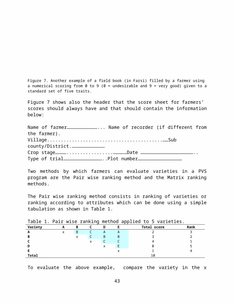
grow progressively larger plots or to grow the stage 2, 3 and 4 trials in more location and with more farmers.

If the Research Station facilities are not available to the PPB program, the responsibility for seed production can be taken up by one of the farmers. In situations where few farmers owns relatively large farmers while the majority of farmers owns small farms, the former can take the responsibility for seed production on behalf of the entire community.

Figure 14. An example of a stage 4 trial with 4 entries and 3 replications arranged in an RCB design with each replication being hosted by a different farmer. The numbers indicate the entry sequence. This design applies well to PVS.

Assuming that a relatively large amount of seed is available for the lines selected from stage 3 and to be planted in stage 4 (25-50 kg in the case of cereal crops), the design that is suggested is the randomized block design, in which each farmers plants only one replications (Fig. 14) and with the largest possible plot size that the amount of seed available allows. In this way stage 4 will provide one more set of data to be used to decide which line(s) deserve(s) to become a variety and at the same time will produce a sufficient amount of seed for a wider distribution of the variety. The layout shown in Figure 14 can be easily used in PVS trials. Preparation of Data Files and Data Entry

An efficient system of data capturing and storing is essential in any breeding program and even more so in a PPB program where the data can be collected by different stakeholders at different times and with different styles. All the data which are collected must eventually be stored in a central filing system that, when completed at the end of the cropping season, is

43

shared with all the stakeholders.

In addition to specific breeding software such as AGROBASE, breeding data can be conveniently entered in Excel.

For all the type of trials we suggest to keep one file which contains all the entries in addition to separate files for each location to be used for the analyses. All the files of the trials of the same breeding stage will all be in the same directory so that all the data of a breeding program in a given country, in a given crop and in a given year will be in one directory.

Two examples of these files are shown in Figure 15 in the case of a stage 1 trial in which the same the entries are planted in all the locations and in Figure 16 in the case of a stage 1 trial in which the entries vary in different locations.

Figure 15. An example of a file (we only show the first and the last 10 entries) used in a stage 1 PPB trial in the case of a country where the same entries are planted in all the locations.

The files have a standard structure: a unique genotype identification number (we suggest to use the number used in the seed multiplication plots on station or on farm for reasons that will be clearer later), entry name, pedigree, source and source number (the number of these last two columns depends on the number of years the material has been on station before being used in the stage 1 trials). The data collected on station (for example

44

on disease and insect resistance) can also be part of the file. In crops such as barley where row type (2 row and 6 row coded as 2 and 6) and seed color (B = black and W = white) may considerably affect farmers’ preferences are also noted in the file. The right side of the file contains the information about the villages in which the various entries are planted. In the case of Figure 15 all the entries are planted in all the 9 villages, while in the case of Figure 16, although 160 entries are planted in each of the 7 villages (see totals on the bottom of columns CF to CL), the actual entries planted in each village differ as shown by the totals in column CM.

Figure 16. An example of a file (we only show some of the entries) used in a stage 1 PPB trial in the case of a country where different entries are planted in different locations.

The presence/absence of a given entry in the column corresponding to a given location is indicated by 1/0 respectively. Therefore, the list of entries planted, for example, in location AZ09 is simply obtained by sorting column CF in descending order and this is in fact is the first step in the preparation of the data files. This will result in 9 files in case of the stage 1 trial shown in Fig. 15 and in 7 files in case of the stage 1 trial shown in Fig. 16. It is obvious that in a case like the one in Fig. 15 the entry number of a given genotype in each of the 9 locations will be the same as the unique identification number (FIT09INCJO). However, in a case like the one in Fig 16 this will not be true and the same entry number in two different locations may actually refer to different genotypes which can then only be identified by using the unique identification number (FIT09IN).

45

Files such as those shown in Figures 15 and 16 are also very useful for the preparation of the seed for planting, particularly in the case when different seed rates are used in the same village. To do this is sufficient to add a number of columns equal to the number of locations with the amount of seed needed for each entry in each village instead of the 1’s. The marginal totals of these columns will be the amount of seed needed for that entry in the trials. After adding the amount of seed needed for the seed multiplication plots we will have the total amount of seed needed. Once the individual file for each individual location is ready, the next step is to randomize the entry in each location.

Randomization

The randomization allows the unbiased assignment of treatments to experimental units and is a prerequisite for a correct estimate of the experimental error. One of the most common mistakes in agricultural research is to avoid the randomization in the first replication where the plot order follows the entry order which is statistically incorrect.

Randomization can be done with various programs or manually. A free and friendly MSDOS software is ALPHANAL produced by the Scottish Agricultural Statistics Service. Although designed for alpha-designs (incomplete block designs) it can be conveniently used also for the randomization of unreplicated trials. The program contains two commands, ALPHAGEN AND ALPHANAL for the generation of randomizations plans and for data analysis, respectively. Its limits are 500 entries and 20 plots per incomplete blocks. Figure 17 shows the main steps in using the program in the case of a trial with 160 entries in 200 plots.

46

Figure 17. Main steps in the randomization of an unreplicated stage 1 PPB trial with 160 entries and 200 plots using the command ALPHAGEN in ALPHANAL.

To use ALPHAGEN for the randomization of an unreplicated trials we consider the locations as replication, and the total number of plots as treatments (= entries). In deciding the number of plots per incomplete blocks one should have already in mind the layout of the trial and in the case of a 50 columns and 4 rows arrangements can be either 5 or 10 because 50 cannot be divided by 20 and 25 is above the limits of the program.

Once the parameters of the trials are fixed, the program uses an iterative process to find the most efficient design and eventually produces a randomization plan which can be stored with a given name.

In the case of replicated trials as those in stage 2, 3 and 4 and regardless of whether the trials are a physical unit as in Fig 13, or either the incomplete blocks or the replications are separate entities planted by different farmers (Fig 14), the randomization follows the same process as shown in Figure 17 with one difference as shown in Figure 18.

47

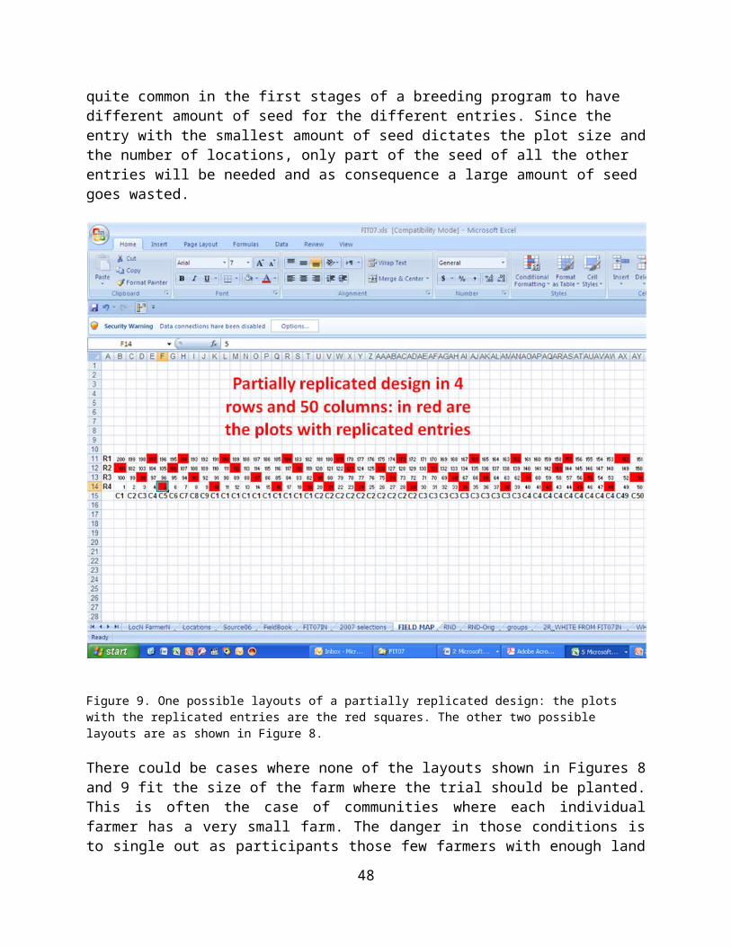
Figure 18. Main steps in the randomization of a replicated stage 2 or 3 or 4 PPB trial with 2 replications, 12 entries and incomplete blocks of size 4 using the command ALPHAGEN in ALPHANAL. The trial is grown by 3 farmers.

Assuming a stage 3 trial with 12 entries to be grown with 2 replications and 3 farmers, we will need to enter as number of replications 6 = number of farmers x number of replications in each farmers field. The full randomization plan is shown in Figure 19. The number of incomplete blocks in this case could have been either 2 or 3 or 4 or 6. Small incomplete blocks are usually associated with a greater precision but one has also to consider possible restrictions imposed by farmers’ field shape because it is not possible to break the physical unity of an incomplete block.

Farmer 1 Replication 1 10 9 12 3 4 2 11 6 5 8 7 1

Farmer 1 Replication 2 10 11 8 1 5 3 12 6 7 9 2 4

Farmer 2 Replication 1 4 3 7 5 6 11 1 12 9 8 10 2

48

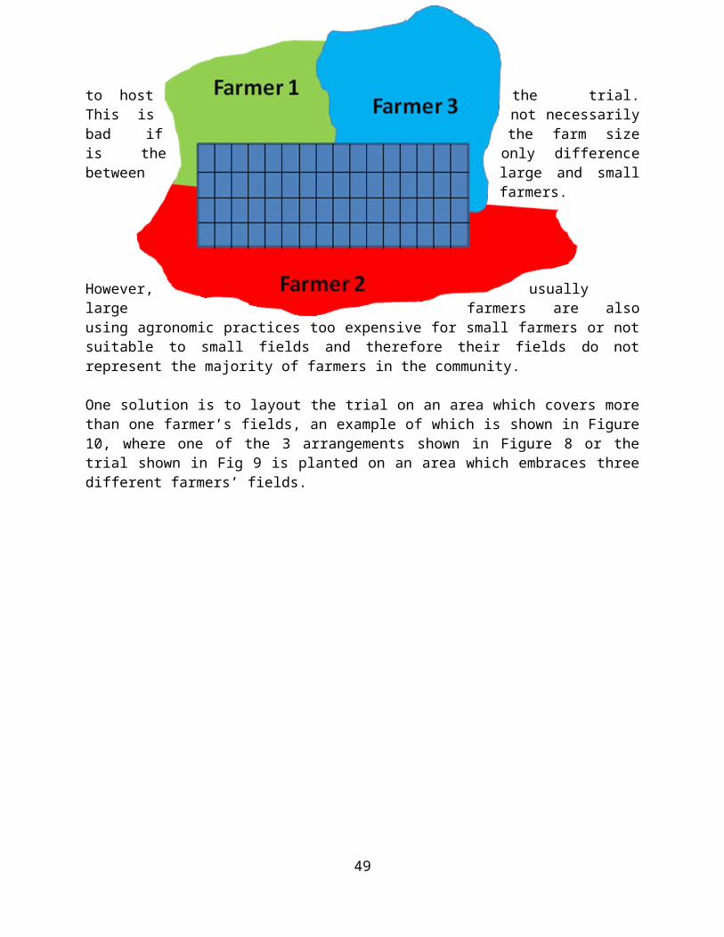
Farmer 2 Replication 2 7 3 8 1110 12 2 5 9 1 6 4

Farmer 3 Replication 1 9 8 3 6 5 10 4 1 2 12 11 7

Farmer 3 Replication 1 8 6 5 211 10 3 4 9 7 1 12

Figure 19. An example of a stage 3 PPB trials using an incomplete block design with 12 entries, 2 replications, incomplete blocks of size 4 planted by 3 farmers in one location.

Preparation of a File for Data Recording

Unreplicated or partially replicated trials

The randomization plan, like the one shown in Fig. 11, can be open with Word and imported in the Excel file keeping in mind that each replication corresponds to a different location, and that the numbers that appear in the randomization files are entry numbers. Therefore, using always the example with 160 entries and 200 plots, one should proceed as follows:

1. Open the file which correspond to a given location;2. Insert a new sheet which we usually named "fldbook" (an abbreviation for

field book) – this will eventually be the sheet for the data entry; the first sheet is usually named entries (Figure 20);

3. Enter a column with the heeder "plot" and fill it with numbers from 1 to 200;

4. Import one of the randomization files and with "paste special and transpose" create a column with entry numbers (header = entry) close to the column with plot numbers. During this operation one should always remember that the plot numbers always start from the left of the randomization plan. In other words, the rows in the randomization plan become stacked columns under the header entry;

5. Sort the file by ascending order for the column "entry". Since we actually have only 160 entries and not 200, we will need to modify this column. The modification depends on whether the trial is using systematic checks or is partially replicated;

a) Systematic checks: let’s suppose that we are using two systematic checks which are entry 159 and entry 160 like the example shown in Fig 15. In this case we will replace, in the column entry, all the entry numbers from 161 to 180 with 159 and the corresponding plots will receive the entry BALADI (the local check). Similarly, we will replace the entry numbers from 181 to 200 with 160 and the corresponding plots with receive the entry RUM (the improved

49

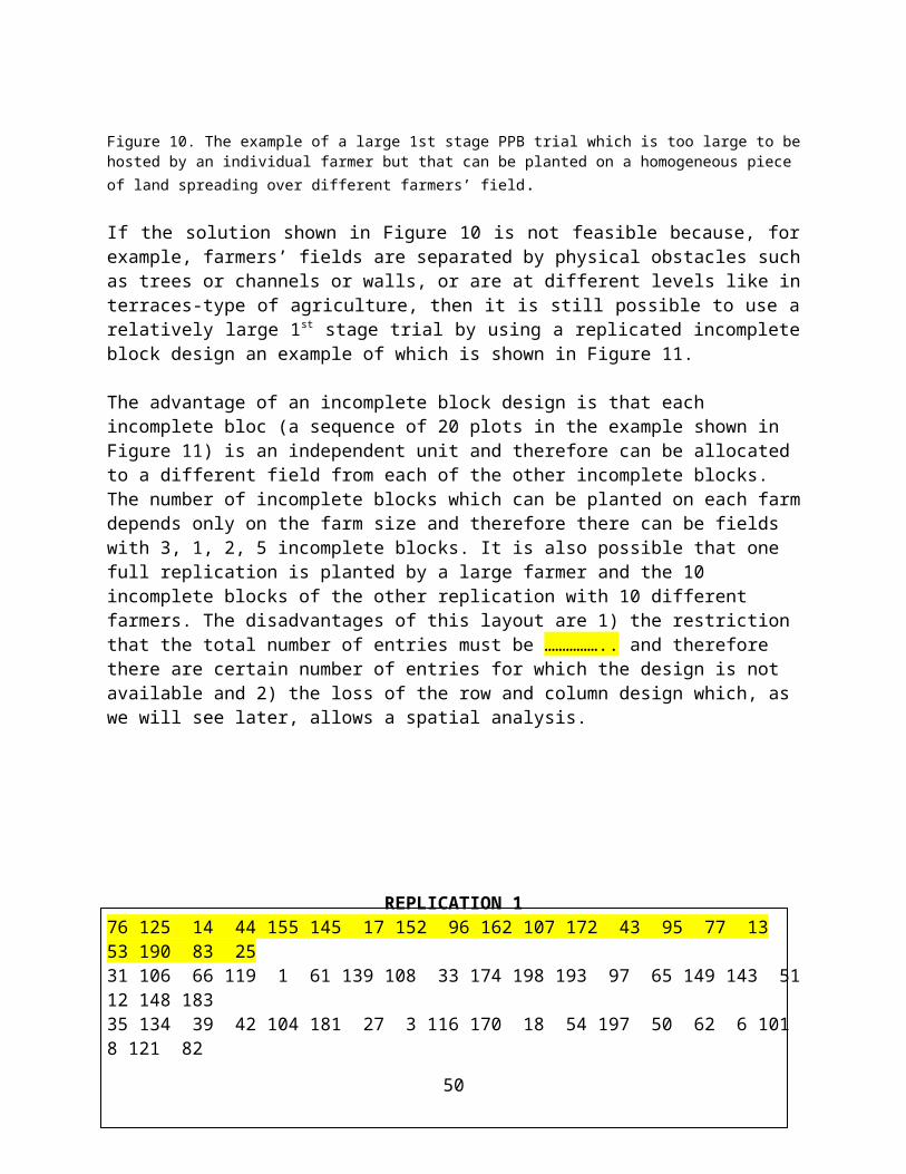
check);b) Partially replicated design: in this case the entry numbers from 161

to 200 are replaced by the entry numbers of the 40 entries (with entry number < or = 160) for which there is enough seed to plant two plots;

6. Once step 5 is completed and regardless whether we used option a) or b) we copy the relevant columns from the sheet "entry" into the sheet "fldbook" making sure that the names are matching with the entry numbers; for the reasons explained earlier it is very important to copy also the column with the unique identification number. All these columns should be pasted at the right side of the column "entry";

7. Sort the file by ascending order for the column "plot";8. Insert three new columns: The first named "trial" with a unique numerical

value indicating the village to be inserted at the left of the column "plot" and two named "row" and "column" to be inserted between "plot" and "entry";

9. Fill "row" and "column" according to the layout as indicated in Figure 8 and 9;

10.Repeat steps 1 to 9 for every location.

Replicated trials

The randomization plan, an example of which is shown in Fig. 19, can be imported in the Excel file following the steps 1 to 10 above with the following differences (shown in bold):

1. Open the file which correspond to a given location;2. Open a new sheet which we usually named "fldbook" (an abbreviation for

field book) – this will eventually be the sheet for the data entry; the first sheet is usually named entry;

3. Enter a column with the heeder "plot" and fill it with numbers from 1 to 24 (12 entries x 2 replications) three times one below each other, for each of the three farmers;

4. Import the randomization file and with "paste special and transpose" create a column with entry numbers (header = entry) close to the column with plot numbers. During this operation one should always remember that the plot numbers always start from the left of the randomization plan. In other words, the rows in the randomization plan become stacked columns under the header entry;

5. Sort the file by ascending order for the column "entry";6. Once step 5 is completed we copy the relevant columns from the

sheet "entry" into the sheet "fldbook" six time, once for each replication and each farmer. All these columns should be pasted at the right side of the column "entry";

7. Sort the file by ascending order for the column "plot"

50

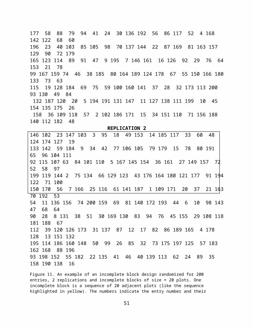
The next steps will depend on whether the trial is a physical unit or not. If the trial is a physical unit then the steps to follow are (Figure 21):

8. Insert five new columns: The first named "farmer" with a numerical value indicating the farmer (in our example will be 1 for rows 2 to 25 – row 1 is the header - , 2 for rows 26 to 49 and 3 for rows 50 to 73) to be inserted at the left of the column "plot" and four named "block", "sblock", "row" and "column" to be inserted between "plot" and "entry". The column "block" has to be filled with the code for replication (in our example will be 1 for rows 2 to 13, 26 to 37, 50 to 61 and 2 for rows 14 to 25, 38 to 49, 62 to 73) and the column "sblock" has to be filled with the code for the incomplete blocks (in our example the values are from 1 to 6 for each farmer);

9. Fill "row" and "column" according to the layout as indicated in Figure 13.

If the trial is not a physical unit then the steps to follow are (Figure 22):

8. Insert three new columns: The first named "trial" with the numerical code for the village, the second named "farmer" with a numerical value indicating the farmer (in our example will be 1 for rows 2 to 25 – row 1 is the header - , 2 for rows 26 to 49 and 3 for rows 50 to 73) to be inserted at the left of the column "plot" and the third named "block" to be filled with the code for replication (in our example will be 1 for rows 2 to 13, 26 to 37, 50 to 61 and 2 for rows 14 to 25, 38 to 49, 62 to 73);

As we will see later the column "plots" is not required for the analysis but it is useful to keep it in the "fldbook" to facilitate data collection.

The preparation of the file, in this case a text file, is much simpler if the data will be analyzed with ALPHANAL, and this will be illustrated in the section on data analysis.

Data Entry

The sheet "fldbook" prepared according to the steps listed above can be printed for the manual data recording in the field or in the lab, or can be saved in a palmtop for the electronic recording of the data.

In the first case the data have to be entered manually in the sheet "fldbook" while in the second they will be transferred by connecting the palmtop to the desktop or the laptop. In either case it is strongly recommended that the data be transferred IMMEDIATELY AFTER BEING COLLECTED FROM THE FIELD. Once entered in the computer, it is suggested to calculate minimum and maximum or to rank them to verify that there are no obvious mistakes.

51

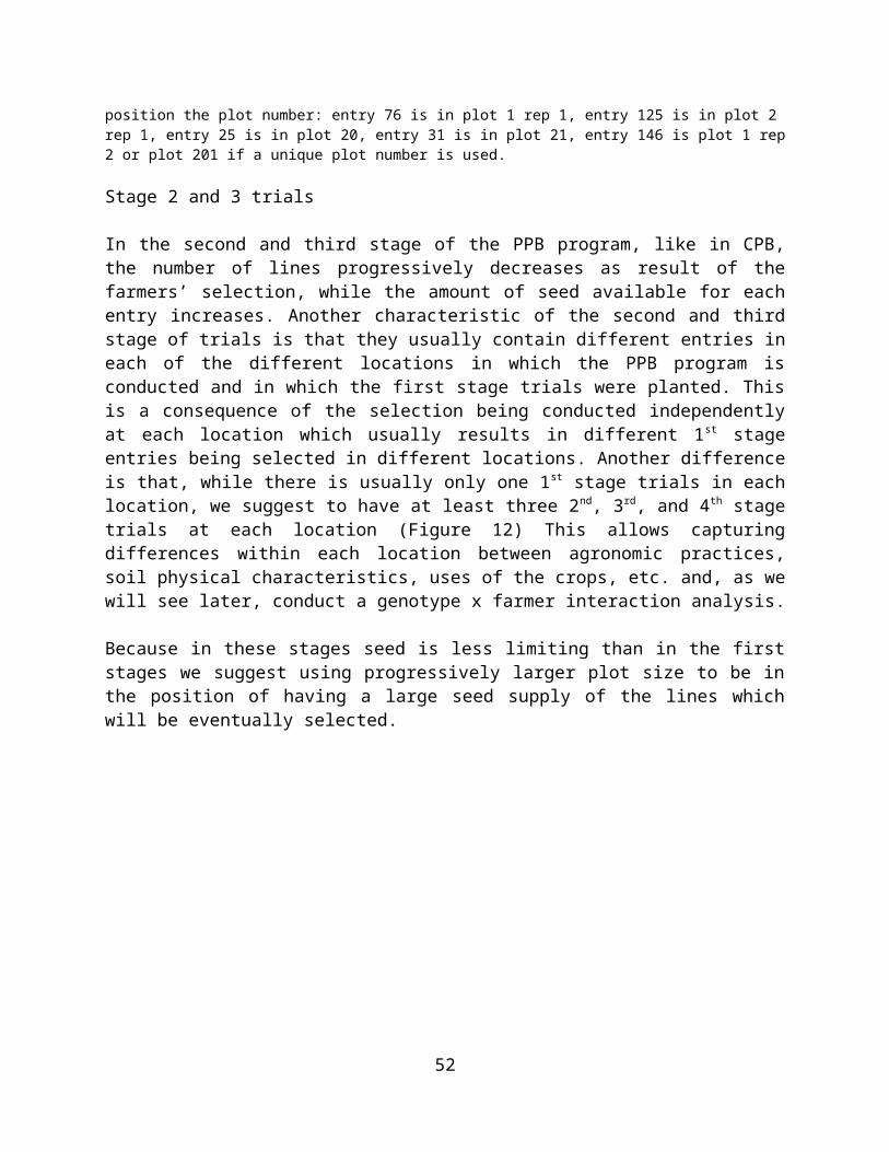
Even better is to analyze them because this can easily reveal mistakes either in recording the data from the field or in entering them manually. A mistake discovered when the crop is still in the field can be easily fixed by going back to the field and by measuring again the plot(s) with value(s) which look suspicious.

In the "fldbook" sheet is important to enter all the details about the measurements such as units (m, cm, mm, m2, cm2, mm2, kg, g, etc), date of data recording etc. In the case of the yield data it is recommended to enter a column with the plot size, given that it may happen that in some plots the area harvested may be different from the majority of the other plots. The principle in organizing this important sheet in the file is that it should be as transparent as possible to whoever need to use the file. Examples of the "fldbook" sheet in a data file of an unreplicated trial (stage 1) and of a replicated trial (stage 3) are given in Figures 20 and 21,

respectively.Figure 20. An example of a fieldbook sheet in a data file of a stage 1 PPB trial with 160 entries and 200 plots in 4 rows and 60 columns.

A number of features shown in the two Figures are worth mentioning. Firstly, it will be noticed that the entry number (columns G in Figure 20 and I in Figure 21) does not necessarily correspond to the unique identification number of the genotype (column H in Figure 20 and J in Figure 21) for the

52

reasons mentioned before. Secondly, as one of characters which are important to farmers in the case of barley (and presumably also of other cereals) is spike length, we take two measures of plant height, one from ground level to the bottom of the spike (PlHt_B_cm), one from ground level to top of the spike excluding the awns (PlHt_T_cm); spike length (SL_cm) is then derived with a formula (column P – column O). This method does not have any advantage in case di manual note taking. However, in the case of electronic capturing of the data, the spike length is calculated plot by plot as the other two measures are recorded as an additional way to check the data. Thirdly, grain yield is recorded on one sample of 1.6 m2 as g/plot in stage 1 trial (column R) and on two samples (because of larger plots) of 1.6 m2 in stage 3 trial (columns T and U). Grain yield in Kg/ha (columns T and W, respectively) is obtained by dividing column R by plot size (column S) and multiplying by 10 in stage 1 trials and by dividing the mean of the two samples by the plot size in stage 3 trial.

Figure 21. An example of a fieldbook sheet in a data file of a stage 3 PPB trial with 12 entries, 2 replications, 6 incomplete blocks of size 4 and 3 farmers. In each farmer’s field the layout is 2 rows and 12 columns.

Columns U to AD and X to AG contain the scores (from 0 = bad to 4 = very good) given by individual farmers (in this case 10, but the number is obviously variable from village to village), and their average (FS) is in columns AF and AH, respectively. Eventually 1000 kernel weight in grams (TKW g) is in column AG in Figure 20 while, since we have two samples for grain yield in stage 3 trial, 1000 kernel weight is measured independently in the two samples (columns AI and AJ) and their mean is in column AK.

53

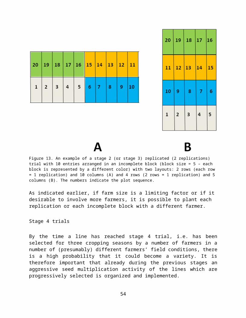
In rows 204 and 205 of Figure 20 and 78 and 79 of Figure 21 are the minimum and maximum for the values in each of the relevant columns. As mentioned earlier this is a powerful and easy way to detect a number of mistakes.

An example of the "fldbook" sheet in a data file of a stage 4 trial with replications planted with different farmers is shown in Figure 22. The structure of the file is considerably simpler that those considered so far. The sheet "fldbook" has one column with the code for the village , one for the plot number, one for the entry number, one for the unique identification number (= plot number in the seed increase), and one for the farmer (which

in this case is equivalent to the replication) code.Figure 22. An example of a "fldbook" sheet in a data file of a stage 4 PPB trial with 9 entries and 2 replications with one replication planted with one farmer and the second with another farmer.

These columns will be followed by those with the data which are similar to those discussed earlier (see Figures 20 and 21) with the difference that, because now the plots are much larger, grain yield and 1000 kernel weight are measured on trhee samples each (columns N, O and P for grain yield in g/plot and columns AE, AF, and AG for 1000 kernel weight in g).

The "fldbook" sheet shown in Figure 22 has to be used also in stage 2 and 3 trials in the case it is not possible to keep the trial as a physical unity.

54

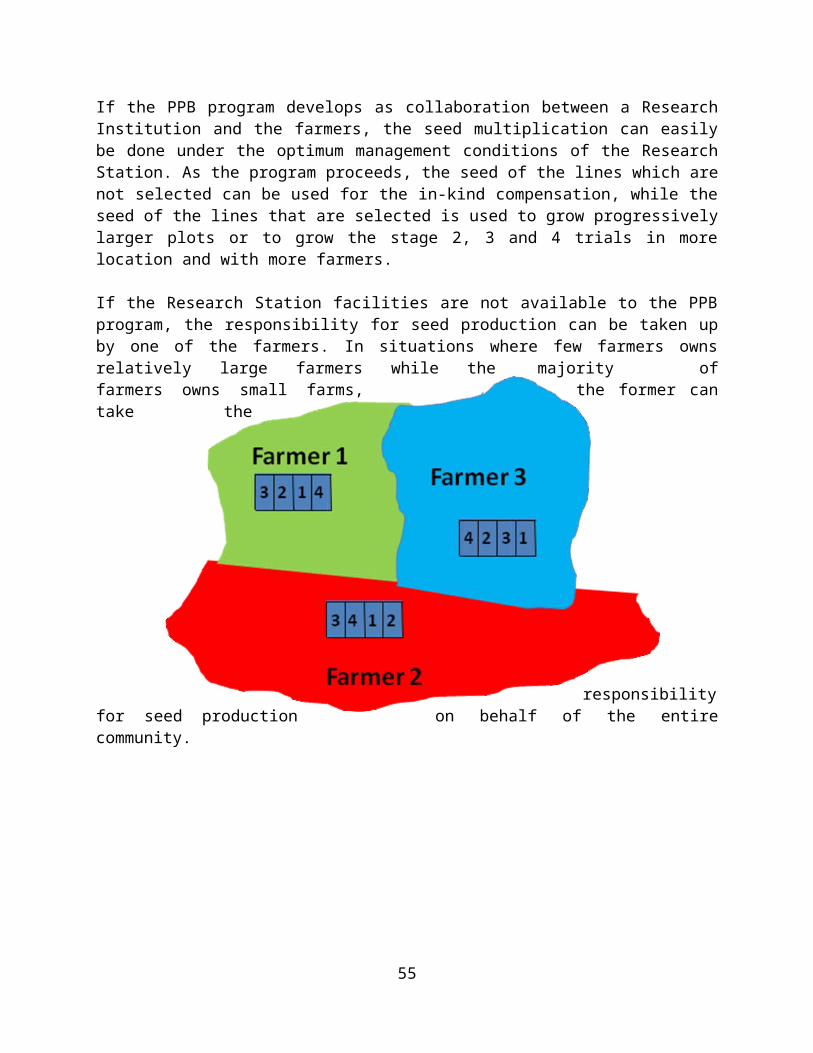
Before leaving this topic, it worth mentioning that is very useful (for reasons that will be clear in the section on data analysis) to:

1. Use the shortest possible abbreviation as header for the variables;2. Use always the same abbreviation for the same variable;3. Use always the same sequence. The actual sequence is important for

plot, row, column and entry but not for the variables. However, once a given sequence for the variables is decided, using always the same sequence saves a lot of work during the subsequent data analysis and data reporting.

The operations described above apply with only minor differences for a range of statistical analysis using GenStat.

Data Storage

Safe data storage is a major issue in plant breeding programs. Examples of strategies that can be used to reduce to a minimum the risk of data loss are frequent backups; storage of data in external disk drives; and storage of data in at least one computer never connected with networks or the Internet to reduce the probability of introducing viruses.

Data Analysis

Updating a File for Data Analysis: unreplicated trials

The sheet for data analysis described below applies to unreplicated trials regardless of the actual field layout (Fig. 8) and regardless of whether there are systematic checks or if the trial is partially replicated (Fig. 9). The sheet for data analysis is prepared from the sheet "fldbook". If the latter has been prepared following the instructions given in the previous section, the operation is straightforward because it consists in copying the following columns in a new sheet: trial, plot, row, col, entry, ph, sl, gy, fs, kw. The sequence of the first five columns is fixed, while the rest vary with the crop, the season, the trial etc. It is important to understand from now that the statistical programs expects to find the trial number, the plot number, the row number, the column number and the entry number IN THIS SEQUENCE in the first five columns REGARDLESS OF THE HEADER. Therefore, the program will run without problems if the first column is called village or farmer instead of trials. Similarly is not important to use Row or rows instead of row, or columns instead of col or genotype instead of entry.

55

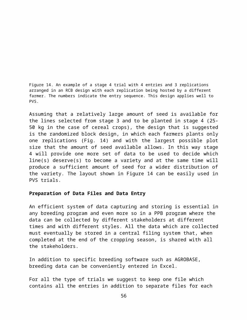
Figure 23. An example of a sheet prepared for data analysis using the field book sheet in Figure 20.

An example of a typical sheet for data analysis is shown in Figure 23: the comparison with Figure 20 will clarify which columns have been copied.

Spatial Analysis of an unreplicated trials

Once the data are prepared as shown in Figure 23, it is possible to proceed to the analysis following the steps below:

1. Open the directory "id_2002006 SPUR Spatial Analysis of Unreplicated Trials". To fully understand the theory behind this section please consult Singh et al. (2003);

2. Open the file "DataSPUR.txt". The first part of the file is simply a set of instructions most of which have been given above. The new instructions are those listed as inputs meaning that these are the changes that the user needs to make in the file before running the analysis:

"--------------------------------------------------------------------------------------------------------------------------------------------------Step 0: Prepare data-file for carrying out Spatial Analysis of data from UnReplicated trials. The texts within the (two matching) double quotes are the comments (ignored by Genstat) to help input the

values of the parameters. Some input names would be mandatory as defined in the program. Save this file as text file. You must include the following identifier/abbreviation for the mandatory variables/vectors (factors) .Vectors/factors TrialNo: column (factor) to represent trial. Geno: column (factor) to represent the genotype. Rows: column (factor) to represent row-position of the plot in the rectangular layout in the field Cols: column (factor) to represent column-position of the plot in the rectangular layout in the field

56

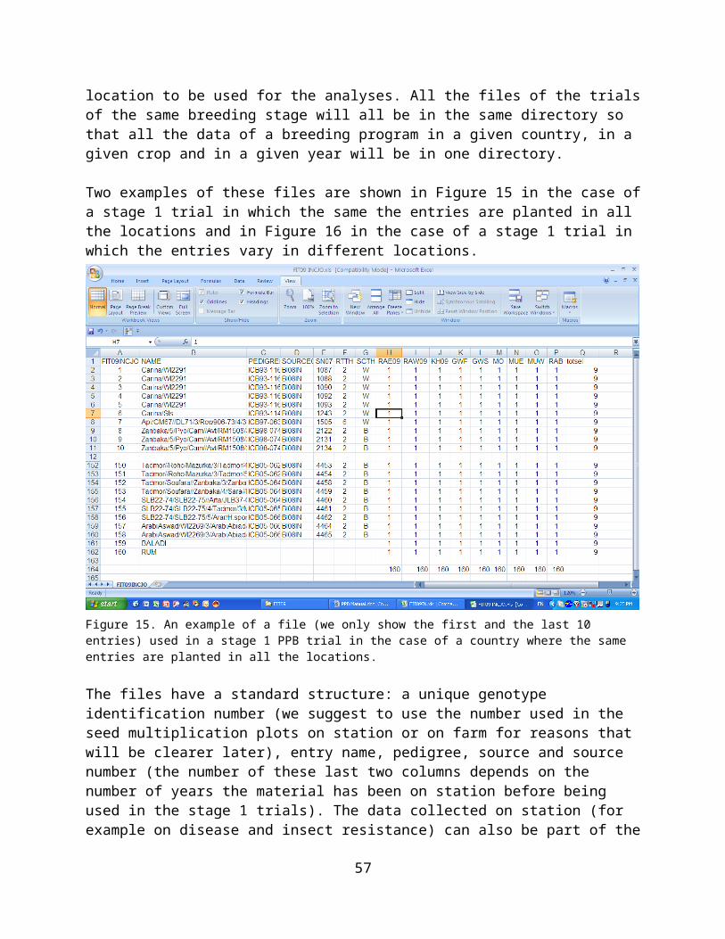
Note: If the layout has more rows than columns (i.e. the number of rows is greater than the number of columns), then designate 1) its rows as Cols, and 2) its columns as Rows in your 3rd input line.

Preparing the file: There are following 3 places of inputting information from your side.1. First input: Choose the set of models you wish to select the best from. If you wish to search from all

the nine models shown in the example, then do not change the line of 1st input, shown in the example, else you may cut and paste from the following list.

Note that the whole list (items separated by commas) should be within single quotes. (models): ' Crd,CrdAr,CrdArAr, CrdL,CrdLAr,CrdLArAr, CrdCS,CrdCSAr,CrdCSArAr ' 2. Second Input: List the variables you wish to analyze; the whole list (items separated by commas) should be

within single quotes. For example: 'phbr, gybr' 3. Third input: list all the variables in the data file to read; the whole list (items separated by commas) should be

within single quotes. For example: TrialNo, Plot, Rows, Cols, Geno, phbr, gybr' 4. Fourth input: place the columns of the data exactly in the same order as in the Second input (Step 3)Warning: a. Please do not put any column of text values. b. All the variables should be as a single word begining with a letter (such as W100Seeds or Yield, but not

as ' W100 Seeds ' ) c. Variables for analysis are in Step 2 (second input), so thay must be exactly same as in Step 3 (third

input), where they are being read for storing data values---------------------------------------------------------------------------------------------------------------------------------------------------- ' Crd,CrdAr,CrdArAr, CrdL,CrdLAr,CrdLArAr, CrdCS,CrdCSAr,CrdCSArAr ' "<-------- List the models you wish

to choose from in this line. (Input 1st of 4 inputs) ---------------------"3. First input (in bold) is usually ignored as it is advisable to let the program

search among all the spatial models available in the module;4. Second input: continuing with our example (Fig. 23), replace the variable

listed between the single quotes before: "<------------ List the variables you wish to analyze in this line. (Input 2nd of 4 inputs) ---------------------" with our variables separated by commas as follows: ‘ph, sl, gy, fs, kw’. Note that this command allows the analysis of a sub set of variables, not necessarily in sequence, for example ‘fs, kw’ if the first three have been already analyzed previously;

5. Third input: replace what is included between the single quotes ' ' before: "<---------- List all the variables in the data file in this line. (Input 3rd of 4 inputs)-------" row 1 of the sheet shown in Figure 23 as follows 'Trial, plot, row, col, entry, ph, sl, gy, fs, kw'. This line is a description of the data file and nothing should be omitted. In addition the variables (ph, sl, gy, fs, kw) are case-sensitive in the sense that the same case should be used in the second and in the third input line. For example entering 'ph' in the second input line and 'Ph' or 'PH' in the third input line will determine an error in reading the file and the program will not run;

6. Fourth (and last) input: replace the old data set with the new data set by simply copying the data (not the header) and pasting them making sure that all the old data are correctly replaced;

7. Save the modified DataSPUR.txt file in the same directory "id_2002006 SPUR Spatial Analysis of Unreplicated Trials".

Before proceeding with the analysis, it should now be clear why it is convenient to use consistently the same abbreviations of the variables and in the same sequence. Let’s suppose that the example above refers to the first of a series of similar data sets all representing stage 1 trials in different villages of the same PPB program. When the data of the second village will be analyzed, and assuming that in each village the same data were collected, only steps 1, 2, 6 and 7 will be necessary as the structure of the

57

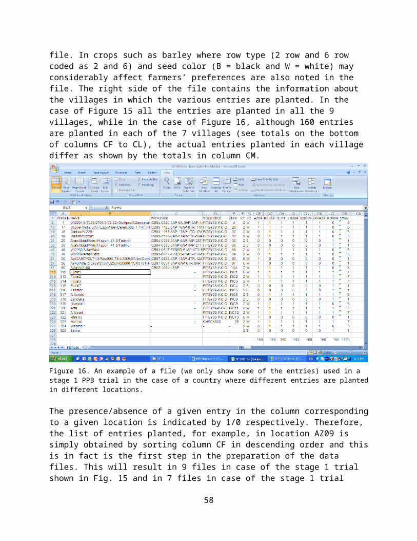
previous file will still be valid. In this way several data sets can be analyzed in a relatively short time.

Once the DataSPUR.txt file has been saved, the analysis proceeds as follows:

8. Start Genstat and select the directory "id_2002006 SPUR Spatial Analysis of Unreplicated Trials". If the default directory is different, use "tools", "working directory", "add", then select id_2002006 SPUR Spatial Analysis of Unreplicated Trials, and "set as".

9. Click "open", double click "Program_Spur.gen" and "submit"10. The GenStat icon will turn red while the program is running. When it

turns green the analysis is completed and the results are stored in the file ReportSPUR.txt

The steps which follow are the same regardless of the data set and the type of analysis and therefore will be presented after two examples of data analysis of replicated trials.

Updating a File for Data Analysis: replicated trials in rows and columns

The sheet for data analysis described below applies to replicated trials of stage 2 and 3 regardless of the actual field layout (Fig. 13) and assuming that the same trial is planted with more than one farmer. It will not apply in all the cases described earlier where the trial is physically subdivided among different farmers.

As illustrated earlier the sheet for data analysis is prepared from the sheet "fldbook" that will be prepared following the instructions given in the previous section. The only difference is the structure of the "fldbook" which now has two more columns ("block" and "sblock") to indicate the replication and the incomplete block, respectively and with the first column using the header "farmer" instead of "trial" (Figure 24).

The same recommendations given earlier concerning the sequence of the columns up to "entry" apply to this case.

Spatial Analysis of a replicated trials in rows and columns

Once the data are prepared as shown in Figure 24, it is possible to proceed to the analysis following the same steps illustrated in the case of the unreplicated trials except that the module for this analysis is in a different directory and therefore the first two steps will be as shown below:

1. Open the directory "id_2002004 SPIB Spatial Analysis Incomplete Blocks".

2. Open the file "DataSPIB.txt". As in the case of the unreplicated trial the

58

first part of the file is simply a set of instructions followed by the input lines, of which the first and the second are exactly the same as in the previous case (the only difference being the list of models).

The third input line differs only because the structure of the file is now different: it will be noticed that the data file expects the first seven columns to contain 'TrialNo, Plot, Rep, Blk, Rows, Cols, Geno, which correspond to Farmer, plot, block, sblock, row, column, entry in the data file in Figure 24.

Figure 24. An example of a sheet prepared for data analysis using the field book sheet in Figure 21

Eventually the final step before the analysis will be:

3. Save the modified DataSPIB.txt file in the same directory "id_2002004 SPIB Spatial Analysis Incomplete Blocks".

Once the DataSPIB.txt file has been saved, the analysis proceeds as follows:

1. Start Genstat and select the directory with "id_2002004 SPIB Spatial Analysis Incomplete Blocks ". If the default directory is different, use "tools", "working directory", "add", then select id_2002006 SPUR Spatial Analysis of Unreplicated Trials, and "set as".

2. Click "open", double click "Program_Spur.gen" and "submit"3. At the of the analysis the results are stored in the file ReportSPIB.txt

59

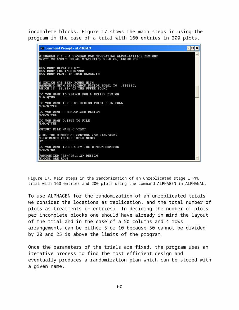
Updating a File for Data Analysis: replicated trials

In this section we will discuss the case of replicated trials such as those of stage 4, with replications planted by different farmers (Figure 14), or trials of stage 2 and 3 when because of limited farm size the trials has to be subdivided and therefore it is not possible to maintain the row and column structure.

The relevant columns for the analysis are shown in Figure 25 together with the variables to be analyzed. It will be noticed that in this case we only need three columns to describe the data set, namely "Trial", "Farmer" and "entry" because the program takes the row sequence as the plot sequence. The other data, the variables, are as in the previous cases.

Figure 25. An example of a sheet prepared for data analysis using the field book sheet in Figure 22.

Spatial Analysis of a replicated trials

Once the data are prepared as in Figure 25, it is possible to proceed to the analysis following the steps below:

1. Open the directory "id_2002001 RCBD (randomized complete block design".

2. Open the file "DataRCBD.txt". As in the previous cases the first part of

60

the file is simply a set of instructions followed by the input lines, which in this case are only three as the one about the spatial models is not included.

Therefore the three input lines correspond to the second, third and fourth input lines described in the case of the unreplicated and replicated trials in rows and columns.

After pasting the data from the sheet shown in Figure 25 the file "DataRCBD.txt" looks like below:

" Step 0: Prepare data-file for analysis of similar trials conducted in Randomised Complete Block Designs in a single treatment-factor.The texts within the (two matching) double quotes are the comments (ignored by Genstat) to help input the values of the parameters. Some input names would be mandatory as defined in the program. Save this file as text file. You must include the following identifiers/abbreviations for the mandatory variables/vectors (factors). Vectors/factors TrialNo: column (factor) to represent trial. Rep: column (factor) to represent replication. Treat: column (factor) to represent the single treatment factor (for example, genotype).

Preparing the file: There are following 3 places of inputting information from your side. 1. First input: list the variables you wish to analyze; the whole list should be within single quotes. for example: ' GYld, DFLR, HSW ' 2. Second input: list all the variables in the data file to read; the whole list should be within single quotes. for example: ' TrialNo, Rep, Treat, DFLR, HSW, GYld' 3. Third input: place the columns of the data exactly in the same order as in the Second input (Step 2)

Warning: a. Please do not put any column of text values. b. All the variables should be as a single word beginning with a letter (such as W100Seeds or Yield, but not as ' W100 Seeds ' ). c. Variables for analysis are in Step 1, so they must be exactly same as in Step 2, where they are being read for storing data values."

'ph, sl, gy, fs, kw' "<------------ List the variables you wish to analyze in this line. (Input 1st of 3 inputs) ------------"

' TrialNo, Rep, Treat, ph, sl, gy, fs, kw' "<------------ List all the variables in the data file in this line. (Input 2nd of 3 inputs) ---"

"Insert columns of your data below in the order of 2nd input line ---- (3rd and the last input) "

21 1 8 42 5 1216.666667 3.666666667 32.521 1 2 52 8 1268.75 3.666666667 29.4166666721 1 6 37 5 1345.833333 3.666666667 38.3333333321 1 4 45 8 1416.666667 4 31.5833333321 1 7 32 5 1095.833333 3 34.3333333321 1 5 31 4 908.3333333 3 32.221 1 3 39 6 1258.333333 4 31.9521 1 9 43 5 1570.833333 4 35.3333333321 1 1 41 7 1081.25 3.333333333 29.4166666721 2 7 28 5 900 2 34.1833333321 2 1 41 5 1035.416667 2.666666667 30.0666666721 2 6 29 4 1131.25 2.666666667 36.9333333321 2 9 32 6 1081.25 2.666666667 35.0833333321 2 3 35 5 1143.75 3.333333333 33.2521 2 4 37 8 1197.916667 4 33.6833333321 2 2 46 8 1145.833333 3.333333333 28.81666667

61

21 2 8 32 7 954.1666667 3 31.8666666721 2 5 27 3 789.5833333 1.333333333 33.06666667

After saving the file the analysis proceeds as follows:

3. Start Genstat and select the directory with "id_2002001 RCBD (randomized complete block design". If the default directory is different, use "tools", "working directory", "add", then select "id_2002001 RCBD (randomized complete block design", and "set as".1. Click "open", double click "Prog RCBD.gen" and "submit"2. At the end of the analysis the results are stored in two files,

ReportRCBDmeans.txt with the means and statistical parameters, and ReportRCBDAnovas.txt with the analysis of variance for each variable.

Importing the Results of the Analysis

The results of the analysis of unreplicated trials and of the replicated trials in rows and columns are stored, as already mentioned, in the files ReportSPUR.txt and ReportSPIB.txt in their respective directories.

The two files have a very similar structure and will be described together, underlining the small differences.

The two files have a header including the date and the time of the analysis: Computer and Biometric Services Unit International Center for Agricultural Research in the Dry Areas (ICARDA) P.O. Box 5466, Aleppo, Syria

Online BioComputing Service Date(D/M/Y) : 4 / 1 / 2010 Time: 10 hr 35 min

This is followed by a description of the file which has just been analyzed: here it has to be noted that the program has been designed to analyse a series of trials with similar structure and this is the reason of the presence of the column "trial".This section in the case of the ReportSPUR.txt is as follows: Summary of the spatial analysis of the data from similar trials conducted in UnReplicated designs .......................................................................................................................................... 1. Trials and parameters of the designs ................................................... No. of similar trials = 1 No. of rows in each trial layout = 4 No. of columns in each trial layout = 50 No. of genotypes = 160 No. of plots in each trial = 200 Variables analyzed: ph, sl, gy, fs, kw Best model searched from: Crd,CrdAr,CrdArAr, CrdL,CrdLAr,CrdLArAr, CrdCS,CrdCSAr,CrdCSArAr

62

In the case of the ReportSPIB.txt is only slightly different:1. Trials and parameters of the designs ................................................... No. of similar trials = 2 No. of rows in each trial layout = 2 No. of columns in each trial layout = 12 No. of replications = 2 No. of incomplete blocks per replications = 6 No. of genotypes = 12 No. of plots in each trial = 24 Variables analyzed: ph, sl, gy, fs, kw Best model searched from : Rcb,RcAr,RcArAr,Lat,LtAr,LtArAr,RcL,RcLAr,RcLArAr,LtL,LtLAr,LtLArAr, RcCS,RcCSAr,RcCSArAr,LtCS,LtCSAr,LtCSArArThe second section (identical in the two files) is a summary of the results. In this section and for each trial and for each variable within each trial, it gives the model selected by the program as best model, the efficiency (in %) over the RCB design, the heritability and the standard error of the heritability. Below this line the file gives for each entry ("Genotype") the Best Linear Unbiased Estimates (BLUE), the Best Linear Unbiased Predictors (BLUPS) and the Unadjusted means................................................................................... 2. Trial-wise summary ............................................................... Trial Variable BestModelNo. ModelTitle Eff% Heritability SE-Heritability21 ph 5 CrdLAr 205.10 0.706 0.064 Genotype BLUE BLUP Unadjusted means

At the bottom of these values the report gives for the BLUE, the BLUPS and the Unadjusted means, the Average Standard Error (Av SE), the Average Standard Error of the Difference (Av SED) and the Coefficient of Variation (CV%). Av SE = 2.422 2.137 3.343Av SED = 3.307 2.842 4.752CV% = 7.95 8.44 8.30

In the case of the replicated trials without spatial analysis the results are stored in two report files, ReportRCBDmeans.txt with the means and statistical parameters, and ReportRCBDAnovas.txt with the analysis of variance for each variable.

The first file has the following structure:Summary of the analysis of the data from similar trials conducted in Randomised Complete Block Designs .......................................................................................................................................... 1. Trials and parameters of the designs ................................................... No. of similar trials = 1 No. of replications = 2 No. of treatments = 9 No. of plots in each trial = 18

63

Variables analyzed: ph, sl, gy, fs, kw .................................................................................... 2. Trial-wise summary Trial = 21 ************************ Means ********************* Treatment no. ph sl gy fs kw 1 41.000 6.000 1058.333 3.000 29.742 2 49.000 8.000 1207.292 3.500 29.117 3 37.000 5.500 1201.042 3.667 32.600 4 41.000 8.000 1307.292 4.000 32.633 5 29.000 3.500 848.958 2.167 32.633 6 33.000 4.500 1238.542 3.167 37.633 7 30.000 5.000 997.917 2.500 34.258 8 37.000 6.000 1085.417 3.333 32.183 9 37.500 5.500 1326.042 3.333 35.208 SE mean = 1.740 0.601 64.207 0.252 0.550 SE difference = 2.461 0.850 90.803 0.356 0.778 LSD at 5% = 5.675 1.960 209.391 0.820 1.794 Grand mean = 37.167 5.778 1141.204 3.185 32.890 Exp. error CV% = 6.621 14.709 7.957 11.168 2.366

**** Statistics from ANOVA ****

Treatment DF = 8 8 8 8 8 F - value = 12.592 6.077 5.915 5.098 22.554 Prob. >= F-val = 0.000855 0.009756 0.010606 0.016651 0.000103 Residual MS = 6.06 0.72 8245.14 0.13 0.61 Residual DF = 8 8 8 8 8 Heritability = 0.853 0.717 0.711 0.672 0.915 SE Heritability = 0.096 0.172 0.175 0.194 0.057

After a description of the structure of the file just analyzed, the ReportRCBDmeans.txt file lists the means for each variable followed by the Standard Error of the mean (SE mean), the Standard Error of the difference (SE difference), the Least Significant Difference at 5% probability (LSD at 5%), the Grand mean, the Coefficient of Variability (Exp. error CV%).

At the bottom of the file, the ReportRCBD.txt lists the statistics derived from the Analysis of variance reported separately in the file ReportRCBDAnovas.txt.

All the information available in the Report files should be be imported into the same Excel files from which we have copied the data. This can be done in several ways using various importing features of Excel.

In the case of the Spatial Analysis we usually import in separate sheets the Models (this includes Efficiency, Heritability and its standard error), the Blues and the Blups as shown in Figures 20 to 24.

To show an example of these three sheets we will use the file of the stage 3 trial shown in Figures 21 and 24.

Figure 26 gives an example of the sheet "models" where we collect the spatial models used in the analysis, the efficiency of the design over the

64

RCBD, the heritability and its standard error and for each trial and each variable from the Report files. It will be recalled that in this case "Trial" stands for Farmer. For each spatial model both the number (as in Table 4 from Singh 2003) and the name of the model are given. It will be noticed that the efficiency of the design is often higher, in some cases much higher, than the RCBD, and that in one case the heritability was zero.

The blues and the blups are imported in two sheets (Figures 27 and 28). which are very similar, containing for each of the entries tested, the entry number, the unique identifier, Name, Pedigree, row type and seed colour, and then for each variable and each farmer, the respective blues and blups. In both cases the bottom rows of the sheets show mean, minimum and maximum, the Table 4. List of models used to describe spatial variability and analysesModel No.

Block Trend Errors (*) Abbreviation

1 Complete I RCB2 Complete AR RCBAr3 Complete ARAR RCBArAr4 Incomplet

eI Lat

5 Incomplete

AR LatAr

6 Incomplete

ARAR LatArAr

7 Complete L I RCBL8 Complete L AR RCBLAr9 Complete L ARAR RCBLArAr10 Incomplet

eL I LatL

11 Incomplete

L AR LatLAr

12 Incomplete

L ARAR LatLArAr

13 Complete LCS I RCBLCS14 Complete LCS AR RCBLCSAr15 Complete LCS ARAR RCBLCSArAr16 Incomplet

eLCS I LatLCS

17 Incomplete

LCS AR LatLCSAr

18 Incomplete

LCS ARAR LatLCSArAr

(*) I: independent plot errors. L: fixed linear trend along rows. CS: random cubic smoothing spline in column number. AR: first order auto-regressive errors along rows; ARAR: first order auto-regressive error along rows and along columns. Lat: Lattice block model. RCB:

65

randomised complete block model (non-spatial).

Figure 26. Sheet used to import the information about the spatial models used in the analysis, the efficiency of the

design over

the RCBD, the

heritability and its standard error. The data are from a stage 3 trial planted by 3 farmers.

66

Figure 27. An example of a sheet used to import the Best Linear Unbiased Estimates of the genotypic values (BLUES) of the entries tested in a stage 3 trial grown by 3 farmers.

Figure 28. An example of a sheet used to import the Best Linear Unbiased Predictors of the genotypic values (BLUPS) of the entries tested in a stage 3 trial grown by 3 farmers.Average Standard Error (Av SE), the Average Standard Error of the Difference (Av SED) and the Coefficient of Variation (CV %).

In the case of stage 1 trials as the one shown in Figure 20, the three sheets

67

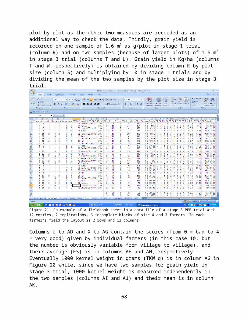
(Models, Blues and Blups) will be the same as described above with the difference that in the sheet "Models" the column Trial indicate the village and that in the sheets "Blues" and "Blups" there will be only one value for each genotype and each variable as the trial is usually grown by only one farmer.

Eventually, in the case of the trials in which the replications are planted by different farmers, the full report as shown in pages 58-59 is imported as such in one sheet of the Excel File.

Discussion of results and farmers’ final selection

Together with the visual selection in the field, the farmers’ final selection is a key activity in a PPB program. It is therefore important to prepare tables which summarize the results in such a transparent way as to make possible for the farmers to decide which entries to select and which entries to discard. These tables differ in the different stages of the PPB program because the amount of information available increases as the entries move from one stage to the next as we will see later.

Stage 1 trials

The first step in summarizing the results of a stage 1 PPB trial for discussion with farmers is to import the Blups in a new sheet ("Table 1" shown in Figure 29) and then, using the command "rank and percentile" under "Data analysis" in Excel, to rank each variable either in ascending or descending order depending on the variable (for example for variables such as those in the file shown in Figure 29 the descending order is the most appropriate but in the case of variables such as heading, maturity and disease susceptibility, the ascending order may be more appropriate if earliness and resistance are the desirable attributes). The ranks are added in the file to the right of the respective variable and they are important because allow farmers to select based on the relative rather than the absolute values.

When the number of entries is large, as in this case, farmers in a number of countries have expressed the desire of facilitating their inspection of the data by preparing two additional summary tables: one with the best 20 entries (12.5 %) for grain yield and the second with the best 20 entries for farmers’ score. Examples of these tables are shown in Figures 30 and 31.

The advantage of these tables is that they allow farmers to evaluate the entries not only for the character for which they excel (grain yield and farmers’ score, respectively) but also for all the other characters that have been measured.

68

Figure 29. The first step of preparing the data for meeting the farmers and discuss the results of a stage 1 of a PPB trial is to copy the blups in a new sheet "Table 1" and rank them.

Figure 30. The 20 highest yielding entries in the stage 1 PPB trial shown in Fig. 29 together with a number of reference varieties (rows 23 – 28), i.e. varieties known or released or already adopted by farmers.

69

Figure 31. The 20 entries with the highest average farmers’ score together with a number of reference varieties (rows 23-31), i.e. varieties known or released or already adopted by farmers.

The tables shown in Figures 30 and 31 also allow farmers to check immediately how precise was their visual selection in identifying the highest yielding entries: the two tables have 4 entries in common (100, 121, 10 and 9) which were therefore among the best 12.5% for both grain yield and farmers’ score. It is also very useful to have in these tables those varieties that farmers know well regardless of their ranking.

The summary tables are not strictly needed and should be prepared only if requested by farmers as it happened in our programs.

Once the three tables have been prepared they need to be translated in the language(s) familiar to the farmers so that they can use them without any external assistance. In the translation is useful to keep the number of decimals to the bare minimum.

During the meeting in which the farmers will eventually make the final selection the researchers should not interfere in the discussion, should avoid any influence on the decisions which are taken, should make sure that the discussion is as smooth as possible and should resolve conflicts in those cases in which the farmers are not in the position to reach a consensus. As the PPB program progresses it is not unusual that, at least in some villages, some farmers develop the ability to lead these discussions which then

70

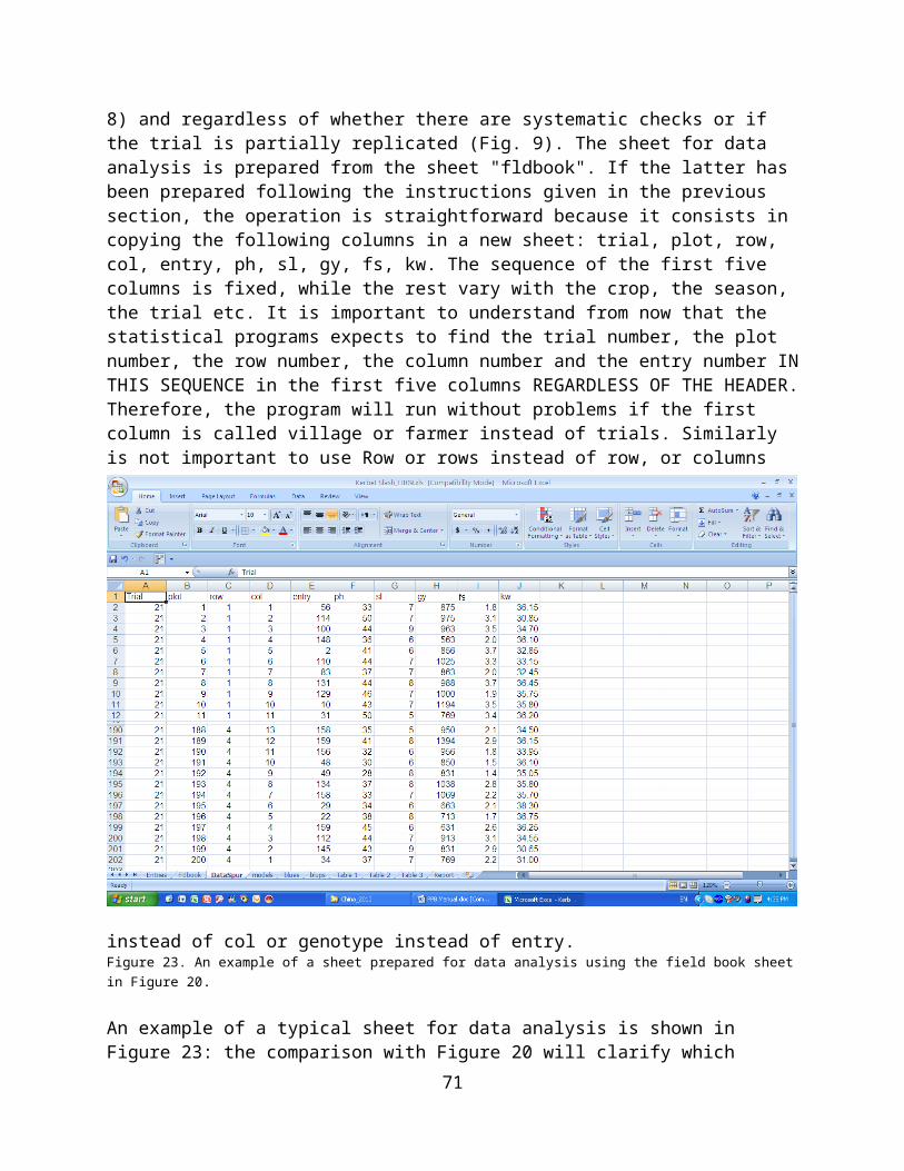
become flexible in terms of timing and certainly become completely independent from any influence of the scientists. It is not within the scope of this manual to analyze the selection criteria used by the farmers, but to show how to properly record the decisions of the farmers. If the selection is made using tables such as those in Figures 30 and 31, the selection of the farmers can be recorded by adding a column of "1" (selected) and "0" (unselected) (Figures 32 and 33).

Figure 32. Figure 30 after farmers’ selection with the additional column "ST 2" (for Stage 2) showing the selected (1) and the discarded entries (0).

71

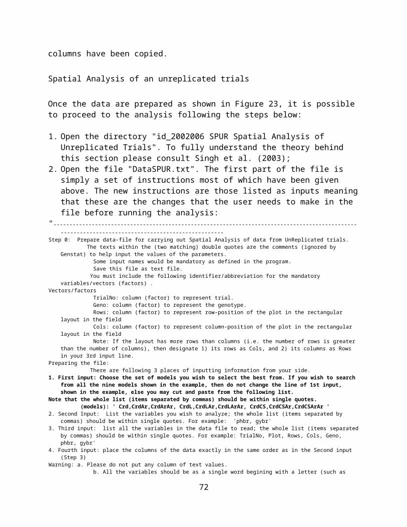
Figure 33. Figure 31 after farmers’ selection with the additional column "ST 2" showing the selected (1) and the discarded entries (0). It will be noticed that 1) the highest yielding entries are not always selected by farmers, and 2) the 4 entries among the best 12.5% for both grain yield and farmers’ score were selected in both tables. The final steps, after the farmers’ selection is concluded are:

1. Transfer the data from column R of Tables 2 and 3 into column R of Table 1;

2. Sort Table 1 for descending order of column R and for ascending order of column B.

The result is shown in Figure 34 with the 17 entries selected by farmers and the three checks (highlighted). These were added because two are PPB varieties already adopted by farmers and one is the popular landrace grown

in the area. Figure 34. The list of the 17 entries promoted from Stage 1 to Stage 2 plus three checks (highlighted).

The sheet shown in Fig. 34 becomes, after few modifications, the first sheet "entries" of the second stage trial to be planted by a given number of farmers in the following year (Figure 35).

72

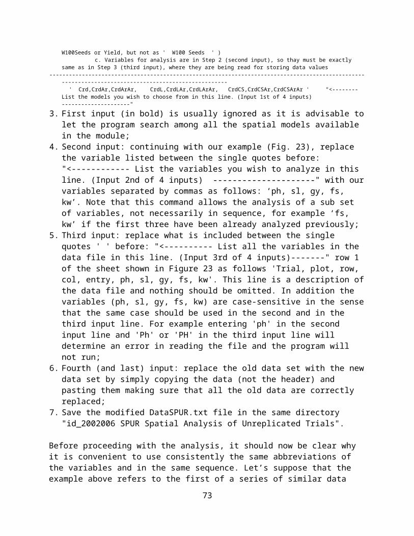
The comparison between Figures 34 and 35 shows that the only

modifications are the replacement of the old column "Entry" with a new one from 1 to 20, and the addition of a new identification number for stage 2 trials in the current cropping season. Figure 35. The new file with the entries promoted from stage 1 to stage 2, with the "fldbook" sheet and the randomization plan (not shown).

The randomization and the preparation of the "fieldbook" sheet will be the first steps to prepare the planting of the stage 2 trials with the entries selected by the farmers.

Stage 2 trials

After having seen the entire process, from the preparation of the tables for discussion with farmers, to the farmers’ selection in a stage 1 trial and to the building of the new file for stage 2 trials, it will be easier to understand that when the same process is applied to the data of stage 2 trials there will be two main differences:

73

1. Data will be available from more than one farmer2. Data will be available from two years (the stage 1 grown in the previous

year and stage 2 grown in the current year)

These differences do not affect the first step which is to copy the blups into a sheet called "Table 1" (Figure 36) which differs from the "Table 1" we have seen in the case of the stage 1 trial because now for each variable we have a value for each of (in this case three) farmers.

Figure 36. The structure of the sheet "Table 1" in the case of a stage 2 trial with 20 entries grown by three farmers.

Before deciding how to finalize the table for the farmers’ selection it is necessary to discuss with the farmers whether they prefer to select on the basis of the results obtained in each farmers’ field or on the basis of the means across farmers.

In the first case it will be necessary to rank the entries (as shown in the case of Table 1 in Figure 29) farmer by farmer, prepare one table for each farmer and proceed as in the case of the stage 1 trial but without preparing tables such as Table 2 and 3 shown earlier because of the limited number of entries.

In the second case, and directly in Table 1, we will first calculate the means of the different variables (columns V, X, Z, AB, AD), then rank them with the procedure illustrated earlier and eventually insert each rank at right side of

74

the respective variable (columns W, Y, AA, AC, AE). The table to translate for the farmers to use during the final selection could be simplified by hiding all the values pertaining to individual farmers (columns G to U) (Figure 36).

The use of averages for selection can be misleading in the case there are large differences between farmers, which is not the case in the example shown in Figure 36 were the average grain yield were 1308, 858 and 630 kg/ha. In case there are large differences between farmers’ fields and for the traits of major interest to farmers, it may be useful to calculate the average of the ranks. Using grain yield as an example, Figure 37 shows the same data of Figure 36 sorted in descending order for the average grain yield across the three farmers’ fields. Entries 15, 18 and 8 are the three highest yielding while entries 6, 19 and 7 are the three lowest yielding.

Figure 37. Difference between ranks for average grain yield and average ranks.

The ranks for grain yield in each of the three farmers’ fields are in columns AY, AZ and BA, and the average of these three ranks are in column BB. By comparing the two columns AW and BB is possible to see that although there is a large coincidence, there are also some differences which in this case are not likely to affect farmers’ selection.

Eventually, the danger of using the averages across farmers as selection criterion can be solved using the GGE biplot software that will be illustrated later.

75

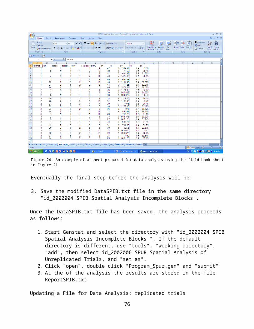
The steps which follow are as described in the case of the stage 1. In discussing with farmers the data of a stage 2 trials, particularly at the beginning of a PPB program, it must be made clear to them that in addition to the choice among selecting on the basis on the performance in individual farmers’ fields or on the basis of the average performance across farmers’ fields, another choice is between selecting on the basis on the data of the stage 2 only or on the basis of the combined data of stage 1 and stage 2. Our experience is that, when the farmers are offered this choice, they prefer to use the combined data. Continuing with our example, the combined data are shown in the sheet "Table 2 (2Y)" (Fig. 38) which contains all the data collected in stage 1 (conducted the year before) as well as all those collected in stage 2. Figure 38 shows the blups collected in the two years and on the right side (shown in Figure 39) the means over the two years (the two Figures are actually the same sheet which has too many columns to fit in one Figure).

76

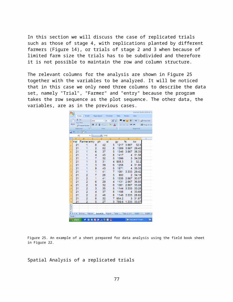
Figure 38. A summary of the 2 years data collected in the first two years (stage 1 and stage 2) of a PPB program. Table 2 (2Y) continues in Figure 38.

Figure 39. The continuation of Table 2 (2Y) with the final selections to be promoted to stage 3 (ST 3).

77

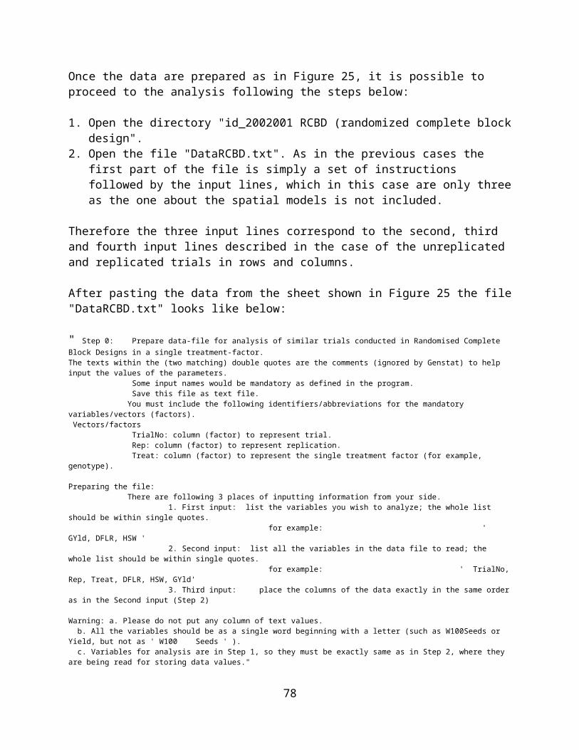
Farmers’ selections are entered in the usual way (1 = selected and 0 = discarded) in the far right column (AQ) name "ST3" (promoted to stage 3) (Fig. 39), the sheet is sorted for this column in descending order and for entry number in ascending order and the resulting file (Figure 40) shows (highlighted) the 9 entries selected to be tested in stage 3 trials in the

following year.Figure 40. The continuation of Table 2 (2Y) with the final selections to be promoted to stage 3 (ST 3).

As in the case of the stage 2 trial, the highlighted portion of the sheet "Table 2 (2Y) of Fig. 40 becomes the sheet "entries" of the stage 3 trial to be planted by a given number of farmers in the following year after replacing the old column "Entry" with a new one and after adding a new identification number for stage 3 trials in the current cropping season. The randomization and the preparation of the "fieldbook" sheet will be the first steps to prepare the planting of the stage 3 trials with the entries selected by the farmers.

Stage 3 trials

The process as illustrated for the stage 2 trials applies to stage 3 trials with the difference that the amount of information available to farmers will be larger and the number of lines lower. In the case of stage 3 trials the farmers will have the choice between 1) selection based on the performance in individual farmers fields in the current cropping season, 2) selection based

78

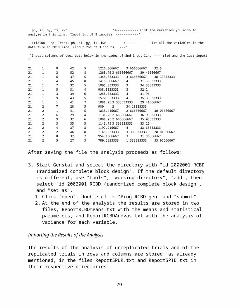
on the average performance across farmers fields in the current cropping season, and 3) selection based on the combined performance in stage 1, stage 2 and stage 3 trials, namely on 3 years data.

The first step which is to copy the blups into a sheet called "Table 1" (Figure 41) which differs from the "Table 1" we have seen in the case of the stage 2 trial only because of a lower number of lines.

Figure 41. The structure of the sheet "Table 1" in the case of a stage 3 trial with 12 entries grown by three farmers.

As shown in Figure 42, in a stage 3 trials we have data from three years, namely the first stage conducted 2 years earlier, stage 2 conducted the year before, and stage 3 conducted in the current year (the data are actually aligned side by side as in Figure 38 and not as shown in Figure 42.

Two points are worth noticing in Figure 42. Firstly, the danger of adding reference varieties or new checks during the course of the same breeding cycle. Entries 6 and 12, which were not included in stage 1 and stage 2 were added only in stage 3. In such a case we can use the new entries as reference for the performance in stage 3 but not as reference to judge the performance across the three cropping seasons, particularly if the means of the three years are substantially different. The second point is about using always the same sequence when entering the variables in a file. For example, if the variables ph, sl, fs, kw and gy were entered in this

79

sequence in stage 1 is very useful to keep the same sequence in stages 2, 3 and 4 because this will make much easier to calculate, with the Excel function "Average" the means across stages.

80

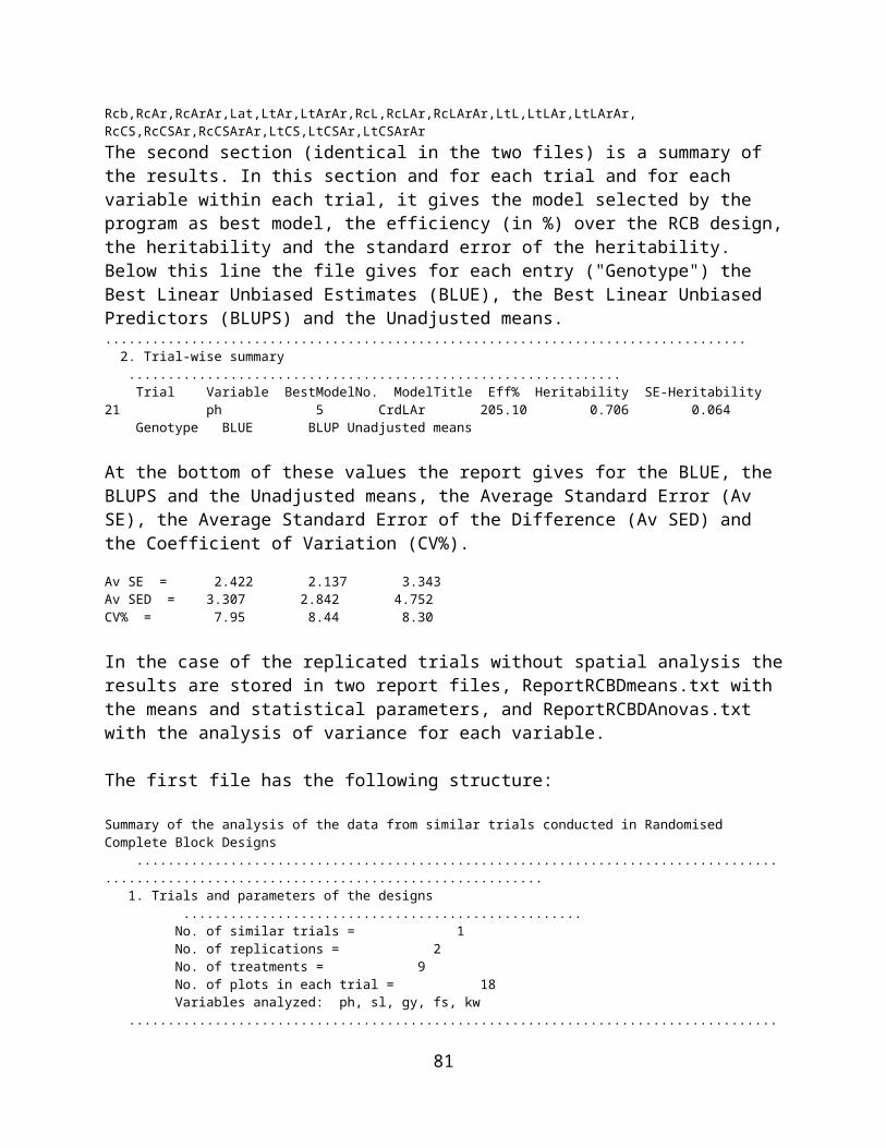
Figure 42. Three years data summarized in the sheet "Table 2 (3Y)" in a stage 3 trial with 12 entries grown by three farmers both in stage 2 and in stage 3.

81

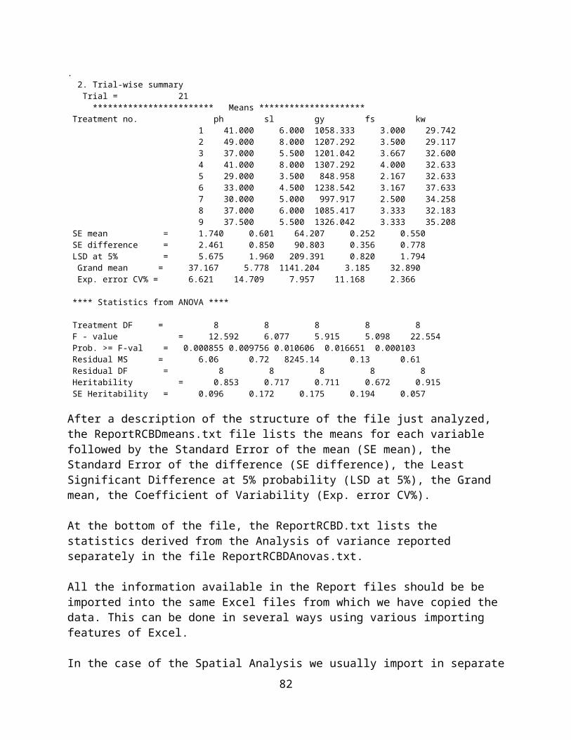
Figure 42. The continuation of "Table 2 (3Y)" with the final selections to be promoted to stage 4 (ST 4).

82

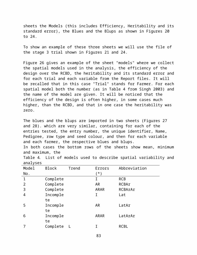
These are reported in Figure 42, together with their rank and the farmers’ final selection in column BG (ST 4). It will be noticed that only 5 of the original 160 entries (entries 3, 4, 5, 7 and 8) have reached the final stage of evaluation. The other entries in the file are checks.

The sheet "Table 2 (3Y)" will be then sorted in descending order for ST 4 and ascending order for Entry: the 9 rows with 1 in the column BG will be copies in the first sheet "Entries" of a new file and after replacing the old column Entry with a new one, adding the identification number for stage 4 trial, and randomizing the entries a number of time equal to the number of farmers growing the stage 4 trial, everything will be ready for preparing the seed and plant.

Stage 4 trials

By the time a PPB program organized as described in pg 11 reaches stage 4, for each entry there are 3 years data and more data are collected in the fourth year. Figure 43 shows the example of Table 1 of a stage 4 trial with four entries and 5 checks grown by 2 farmers (considered as replications)

and analyzed as described in pg 55.Figure 43. "Table 1" of a stage 4 trial with 9 entries (5 of which checks) grown by two farmers used as replication of a RCBD.

In this case not all the entries were tested in all 4 years: in particular entries

83

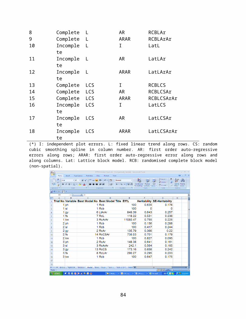
8 and 9 were only tested in stage 1 and stage 4 and therefore they were not considered in the combined data shown in "Table 2 (4Y) (Figure 44).

84

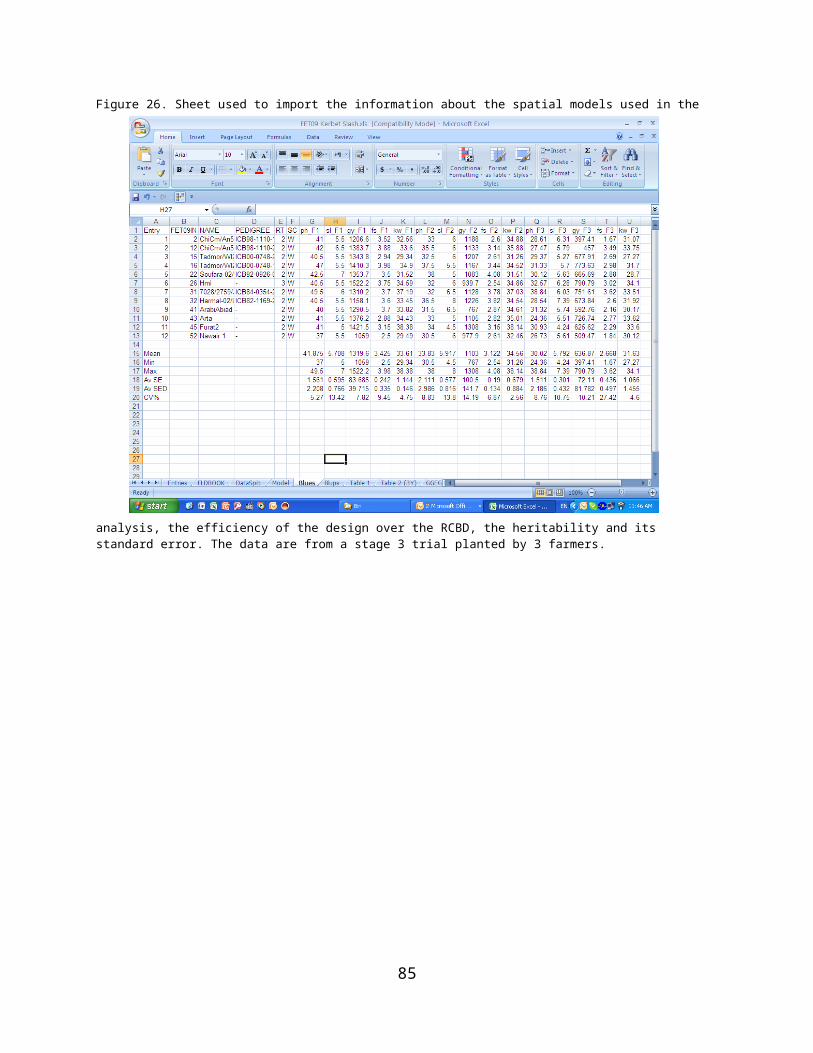
Figure 44. The combined 4 years data in a stage 4 trial with 7 entries (3 of which checks).

85

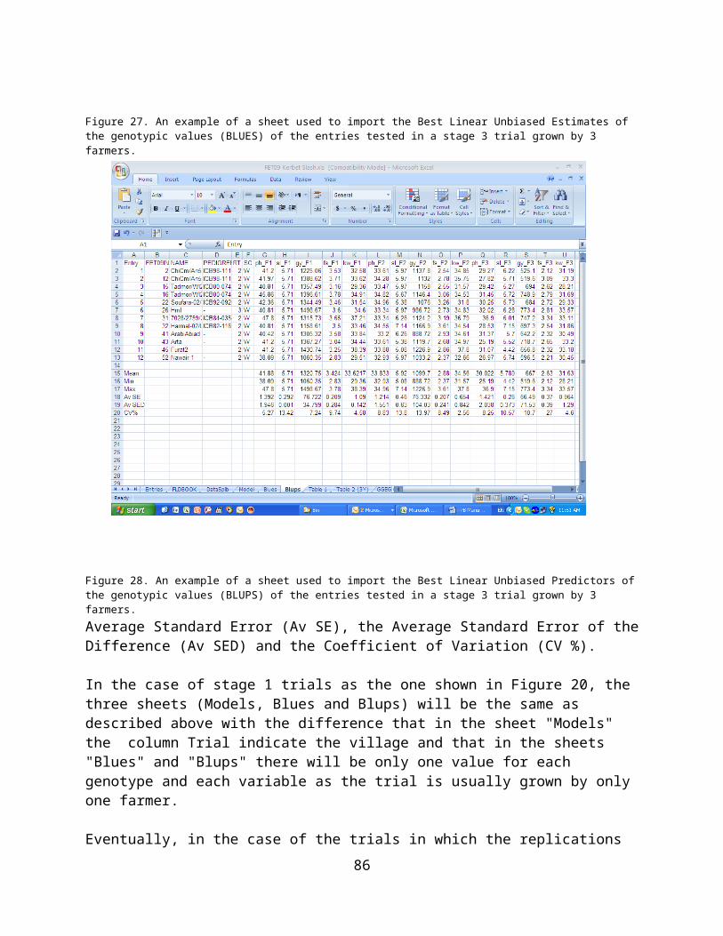
As in the case of Stage 3 combined data, also in this case the four years data are arranged side by side to facilitate the calculation of average which, for the same data shown in Figure 44 are shown in Figure 45.

Figure 45. Four years means and two entries selected and named by farmers as potential varieties at the end of a breeding cycle.

Based on four years data collected in their own field and under their own management, the farmers of the village that we have used as example decided that entries 3 and 4 with yield advantages over both the most common landrace and the improved varieties and with high farmers’ scores, were worth to be considered as potential varieties. Therefore, they were named, as shown in column T, and all the seed available was given to farmers in the village for large scale testing. At the same time these named varieties are included in the crossing program to start a new breeding cycle. In countries were the PPB process is recognized, as it deserves, these varieties could be submitted for release.

Whether they are released or not, it is important to assure that these varieties are accessible to all and that the benefits deriving from their use is shared among all those who have contributed to their development.

Genotype x Environment Interactions

Plant breeding is a complex process and in the majority of cases (the only

86

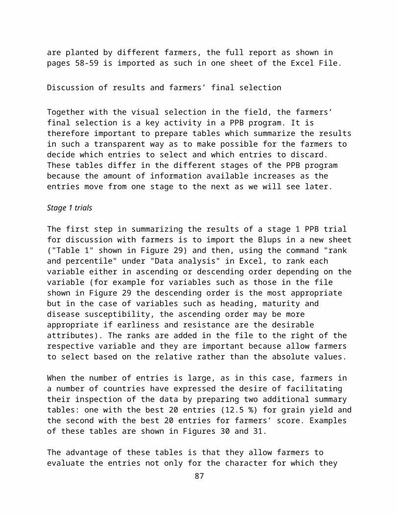
notable exception being the breeding programs in Australia), only a small fraction of it takes place in farmers’ fields: usually most of the process takes place in one, or more often in a number of research stations, and all the decisions are made by the breeders and collaborating scientists (pathologist, entomologist, quality specialists, etc.). One of the main consequences is that a large amount of breeding material is discarded before knowing whether it could have been useful in the real conditions of farmers’ fields, and the one which is selected is likely to perform well in environments similar to the research stations, but not in environments which are very different. This is because of Genotype x Environment (GE) interactions which are one of the major factors limiting the efficiency of breeding programs when they cause a change of ranking between genotypes in different environments (crossover interaction). An example of crossover GE interactions between research stations and farmers fields is given in Figure 146. In both cases there was much more similarity between research stations than between farmers’ fields, and low or negative correlations between research stations and most of the farmers’ fields.

Figure 46. Biplots of thirty barley genotypes grown in six locations in Morocco (left) including two research stations (E3 and E4) and four farmers’ fields (E1, E2, E5 and E6) and of 25 barley genotypes in six locations in Tunisia (right) including two research stations (E5 and E6) and four farmers’ fields (E1, E2, E3 and E4).

In general, when different lines or cultivars of a given crop are evaluated in a sufficiently wide range of environments, GE interactions of crossover type seem to be very common (Ceccarelli et al. 2001). We have argued (Ceccarelli 1989) that for crops grown in environments poorly represented by the research stations, this often results in useful breeding materials being discarded.

When GE interactions are present the plant breeder can ignore them, avoid them or exploit them (Eisemann et al. 1990). When GE interactions are significantly large, it is not possible to ignore them and the two remaining

87

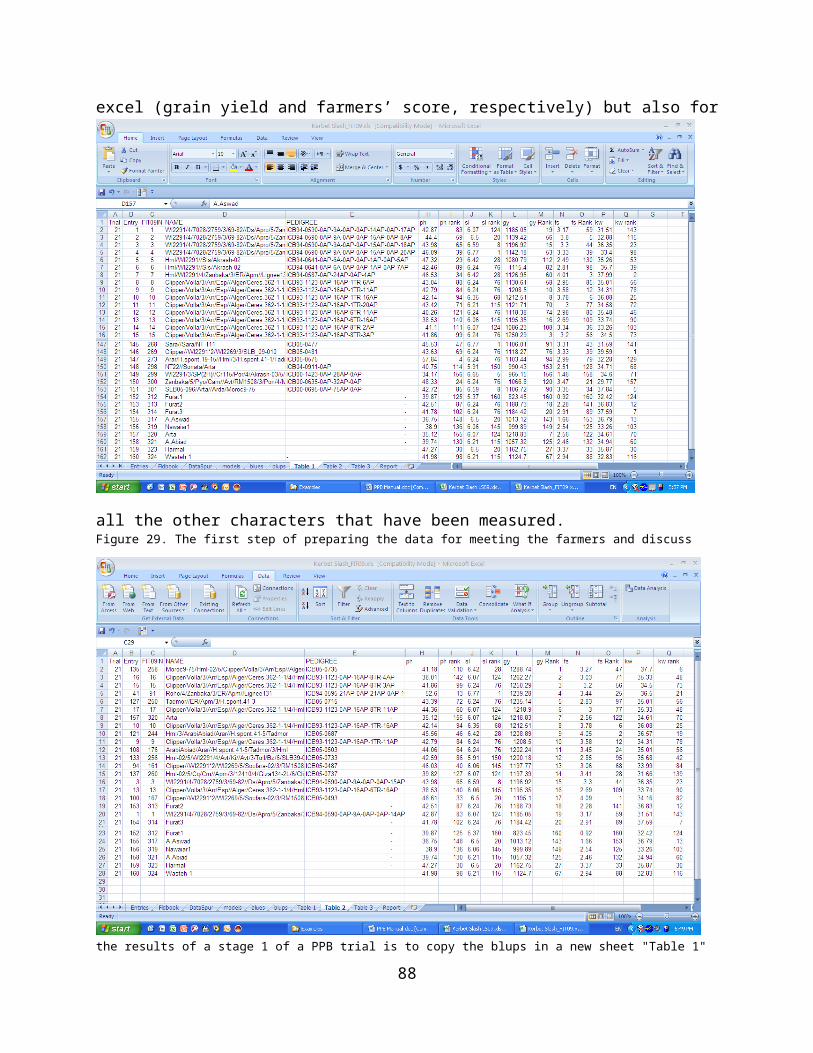
strategies are (1) to avoid them by selecting material that is broadly adapted to the entire range of target

environments, or (2) to exploit them by selecting a range of material, each adapted to a specific environment (Ceccarelli 1989). As mentioned earlier, The choice is based on a separate analysis of the two components of GE interactions, namely Genotype x Years (GY) and Genotype x Locations (GL), the first of which is largely unpredictable, while the second, if repeatable over time, identifies distinct target environments (Annicchiarico et al. 2005, 2006).

One method of analyzing GE interactions is through biplots, which are constructed using the first two principal components (PC1 and PC2) derived by subjecting a two-way (genotypes and environments) matrix, with or without transformation, to singular value decomposition (Yan, 2000); the biplot displays the environments (locations and/or years) as vectors drawn from a common origin (PC1=PC2=0), and the genotypes as points. Similar environments have a small angle (the angle formed between the first vector, the origin and the second vector) between them while dissimilar environments have a large angle between them; similar genotypes have a small angle while dissimilar genotypes have a large angle (the angle formed between the first genotype, the origin and the second genotype). Genotypes far from the origin (e.g. Rihane-03 in Figure 4647a) have a large genotype plus interaction effect. If a given genotype and a given environment vector are on the same side of the origin (e.g. Rihane-03 and BR_96 in Figure 4647a) that genotype performs above average in that environment. By contrast, a genotype which is at the opposite side of an environment vector origin (example Rihane-03 and BO_98 in Figure 4647a) performs below average in that environment. Eventually genotypes close to the origin (Arta and Harmal in Figure 4647b) have an average performance in all environments (Yan et al. 2000).Figure 4647. Biplots of grain yield of seven barley cultivars grown for four years (1995 to 1998) in two dry locations, Bouider (BO) and Breda (BR) with a grand mean of 1.3 t/ha (left) and in two locations, Tel Hadya (TH) and Terbol (TR) with a grand mean of 3.5 t/ha (right).

GGE biplot

88

The use of GGE biplot software will be illustrated using some of the data from the PPB trials utilized earlier in this manual.

The program can process Excel Table of various type, namely 2-way tables (entries and environments), tables containing also the replication hence conducting a full analysis of the row data before the analysis of the GE interaction (three ways tables) and eventually tables containing years, locations and replication. However, the original data are usually analyzed first with one of the methods that were illustrated earlier which, in most case will generate the best linear unbiased predictors (BLUPs) of the genotypic performance. Therefore, the most common situation is to employ the GGEbiplot software to analyze the response of genotypes to various environments using the BLUPs generated bu the previous analysis.

A typical Excel table for GGE biplot analysis is shown in Figure 48 where the rows are the genotypes (entries) and the columns (B to F) are the environments (either years or locations or a combination of both. Missing data can be indicated in various ways. In Figure 48 there are two missing data indicated with asterisks.

Figure 48. A typical 2 ways table for Genotype x Environment Interaction by GGE biplot. The asterix (*) indicate missing data.

89

Figure 49. The start of GGE biplot.

The first steps of the program after clicking Star are to "Open Data" and then to select a Table with the Data File which has been opened (Figure 49). In most cases the table like the one shown in Figure 48 is one sheet of the file, and therefore with the message in Figure 50 the program requests to select the sheet containing the data to analyze.

90

Figure 50. Opening the file.

91

Genotype x Location Interactions in stage 1 trials

Genotype x Location x Year Interactions in stage 2, 3 and 4 trials

Relationships between traits

Farmers’ selection criteria

References

Almekinders C, Hardon J (eds) (2006) Bringing farmers back into breeding. Experiences with participatory plant breeding and challenges for institutionalisation. Agromisa Special 5. Agromisa, Wageningen, The Netherlands. 140 p.

Annicchiarico P, Bellah F, Chiari T (2005) Defining Subregions and Estimating Benefits for a Specific-Adaptation Strategy by Breeding Programs: A Case study. Crop Science 45, 1741–1749.

92

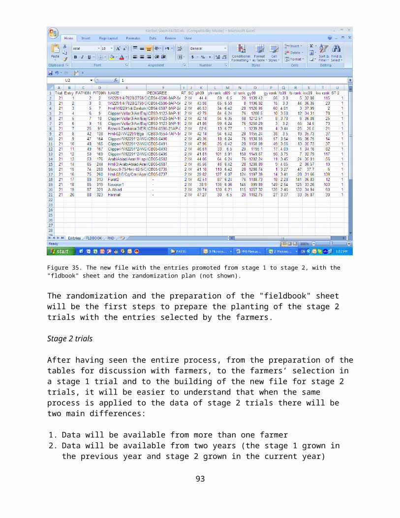
Annicchiarico P, Bellah F, Chiari T (2006) Repeatable Genotype x Location Interaction and its Exploitation by Conventional and GIS-Based Cultivar Recommendation for Durum Wheat in Algeria. European Journal of Agronomy 24, 70–81.

Ashby JA (1990) Evaluating Technology with Farmers: A Handbook. CIAT, Cali, Colombia.

Ashby JA, Lilja N (2004) Participatory research: Does it work? Evidence from Participatory Plant Breeding. In: New Directions for a Diverse Planet. Proceeding of the 4th International Crop Science Congress, Brisbane, Queensland, Australia, 26 September–1 October 2004.

Bellon MR (2006) Crop research to benefit poor farmers in marginal areas of the developing world: a review of technical challenges and tools CAB Reviews: Perspectives in Agriculture, Veterinary Science, Nutrition and Natural Resources, Online ISSN 1749-8848).

Bellon MR, Reeves J (2002) Quantitative analysis of data from participatory methods in plant breeding, Mexico, D.F.: CIMMYT

Byerlee D (1994) Modern varieties, productivity, and sustainability: Recent experiences and emerging challenges. CIMMYT: Mexico, D.F.

Biggs SD, Farrington J (1991) Agricultural research and the rural poor: a review of social science analysis. International Development Research Centre (IDRC), Ottawa, Canada. 139 p.

Ceccarelli S (1989) Wide adaptation. How wide? Euphytica 40, 197–205.Ceccarelli S, Grando S, Tutwiler R, Baha J, Martini AM, Salahieh H, Goodchild

A, Michael M (2000) A methodological study on participatory barley breeding. I. Selection phase. Euphytica 111, 91–104.

Ceccarelli S, Grando S, Singh M, Michael M, Shikho A, Al Issa M, Al Saleh A, Kaleonjy G, Al Ghanem SM, Al Hasan AL, Dalla H, Basha S, Basha T (2003) A methodological study on participatory barley breeding. II. Response to selection. Euphytica 133, 185–200.

Dvorak KA (1987) A social science perspective on evaluating and designing component research: A case study of nitrogen fertilizer and postrainy season sorghum in India. Workshop on Social Science Perspectives in Managing Agricultural Technololgy, 24-27 September 1986, Lahore, Pakistan.

Eisemann, R. L., Cooper, M. and Woodruff, D. R. (1990) Beyond the Analytical Methodology: Better Interpretation and Exploitation of Genotype-by-Environment Interaction in Breeding. In: M. S. Kang (Ed.), Genotype-by-Environment Interaction and Plant Breeding. Department of Agron. Louisiana State Agric Experiment Stn, Baton Rouge, LA. pp. 108–117.

Fehr WR (ed) (1984) Genetic contributions to yield gains of five major crop plants. CSSA Spec. Publ. 7. ASA and CSSA, Madison, WI.

Gepts P Hancock J (2006) The Future of Plant Breeding. Crop Science 46, 1630–1634.

Lilja N, Ashby JA (1999a) Types of participatory research based on locus of decision making. Consultative Group on International Agricultural Research (CGIAR), Participatory Research and Gender Analysis (PRGA).

93

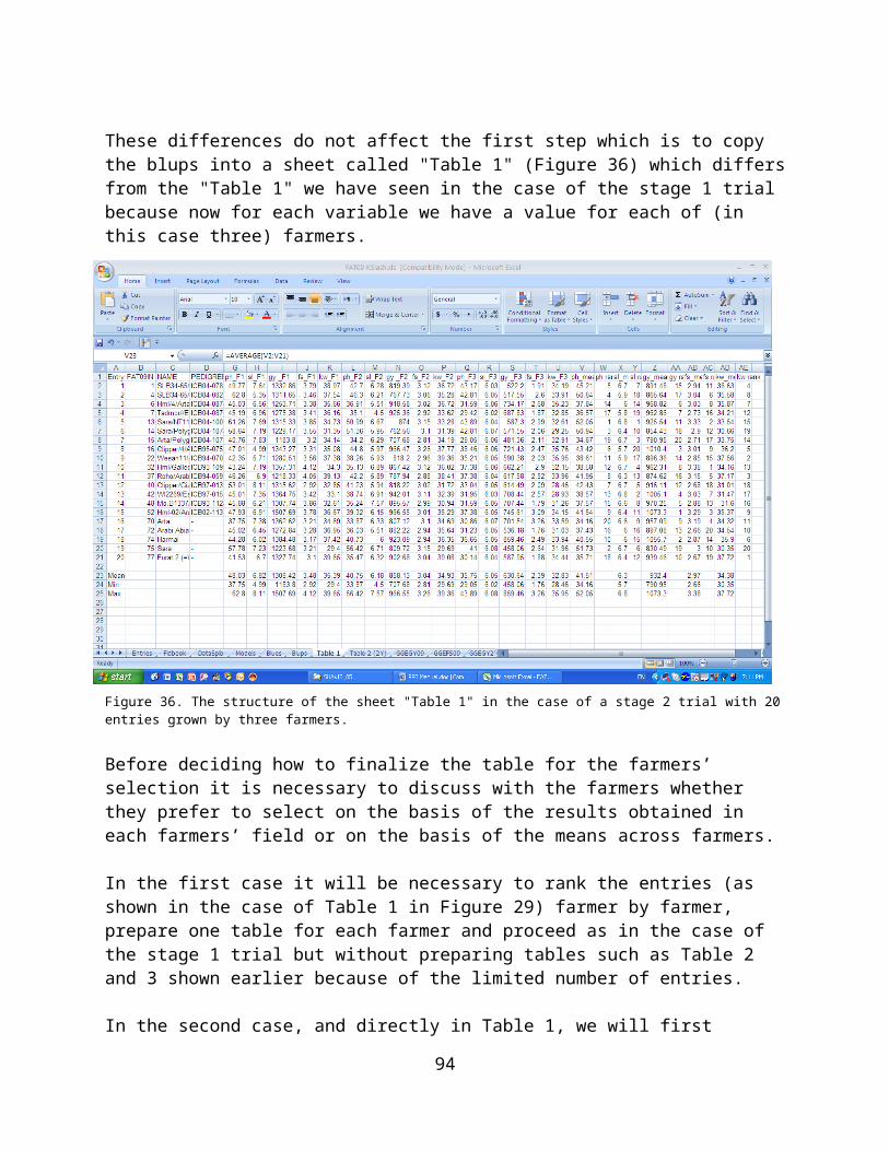
PRGA Working Document No. 6.Lilja N, Ashby JA (1999b) Types of gender analysis in natural resource

management and plant breeding. Consultative Group on International Agricultural Research (CGIAR), Participatory Research and Gender Analysis (PRGA). PRGA Working Document No. 8.

McGuire S, Manicad G, Sperling L (1999) Technical and institutional issues in participatory plant breeding done from the perspective of farmer plant breeding. Working Paper No. 2. CGIAR System-Wide Programme on Participatory Research and Gender Analysis for Technology Development and Institutional Innovation.

Pretty J (1994) Alternative systems of inquiry for sustainable agriculture. IDS Bulletin 25, 37–48.

Joshi KD, Sthapit BR, Witcombe JR (2001) How narrowly adapted are the products of decentralized breeding? The spread of rice varieties from a participatory plant breeding program in Nepal. Eyphytica 122, 589-597.

Ransom C, Drake C, Ando K, Olmstead J (2006) Report of breakout group 1: What kind of training do plant breeders need, and how can we most effectively provide that training? HortScience 41, 53–54.

Rhoades RE and Booth RH (1982) Farmer-back-to-farmer: a model for generating acceptable agricultural technology Agricultural Administration 11, 127-137.

Reynolds MP, Borlaug NE (2006) Impacts of breeding on international collaborative wheat improvement. Journal of Agricultural Science 144, 3 – 17.

Schlegel RHJ (2003) Dictionary of plant breeding. Food Products Press/The Haworth Reference Press, New York.

Schnell FW (1982) A synoptic study of the methods and categories of plant breeding. Z. Pflanzenzüchtung 89, 1 18.

SEARICE (2003) Strengthening farmers’ agricultural diversity management systems. pp. 599–607, in: CIPUPWARD, Conservation and Sustainable Use of Agricultural Biodiversity: A Sourcebook. CIPUPWARD, Los Baños, the Philippines.

Singh M, Malhotra RS, Ceccarelli S, Sarker S, Grando S, Erskine W (2003) Spatial variability models to improve dryland field trials. Experimental Agriculture 39, 1-10.

Soleri D, Cleveland DA, Smith SE, Ceccarelli S, Grando S, Rana RB, Rijal D, Labrada HR (2002) Understanding farmers' knowledge as the basis for collaboration with plant breeders: methodological development and examples from ongoing research in Mexico, Syria, Cuba and Nepal. pp. 19 60, in: D.A. Cleveland and D. Soleri (editors). Farmers, scientists and plant breeding: Integrating Knowledge and Practice. CABI, Wallingford, Oxon, UK.

Walker TS (2007) Participatory Varietal Selection, Participatory Plant Breeding, and Varietal Change. Background paper for the WDR 2008.

Walker TS, Ryan JG (1990) Village and Household Economies in India’s Semi-

94

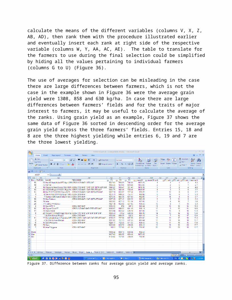
Arid Tropics. Baltimore: Johns Hopkins University Press, 417 p.Weltzien E, Smith ME, Sperling L, Meitzner LS (2000) Technical and

institutional issues in participatory plant breeding done from the perspective of formal plant breeding. Working Paper No. 3. CGIAR Systemwide Programme on Participatory Research and Gender Analysis for Technology Development and Institutional Innovation.

Weltzien E, Smith ME, Meitzner LS, Sperling L (2003) Technical and institutional issues in participatory plant breeding --- from the perspective of formal plant breeding. A global analysis of issues, results, and current experience. PPB Monograph No. 1. PRGA Programme, Cali, Colombia.

Yan W, Hunt LA, Sheng Q, Szlavnics Z (2000) Cultivar evaluation and mega-environment investigation based on the GGE biplot. Crop Sci 40, 597–605

95