poverty, labour markets and trade liberalization in indonesiaftp.iza.org/dp7645.pdf · poverty,...

DI

SC

US

SI

ON

P

AP

ER

S

ER

IE

S

Forschungsinstitut zur Zukunft der ArbeitInstitute for the Study of Labor

Poverty, Labour Markets and Trade Liberalization in Indonesia

IZA DP No. 7645

September 2013

Krisztina Kis-KatosRobert Sparrow

Poverty, Labour Markets and

Trade Liberalization in Indonesia

Krisztina Kis-Katos University of Freiburg

and IZA

Robert Sparrow Australian National University

and IZA

Discussion Paper No. 7645 September 2013

IZA

P.O. Box 7240 53072 Bonn

Germany

Phone: +49-228-3894-0 Fax: +49-228-3894-180

E-mail: [email protected]

Any opinions expressed here are those of the author(s) and not those of IZA. Research published in this series may include views on policy, but the institute itself takes no institutional policy positions. The IZA research network is committed to the IZA Guiding Principles of Research Integrity. The Institute for the Study of Labor (IZA) in Bonn is a local and virtual international research center and a place of communication between science, politics and business. IZA is an independent nonprofit organization supported by Deutsche Post Foundation. The center is associated with the University of Bonn and offers a stimulating research environment through its international network, workshops and conferences, data service, project support, research visits and doctoral program. IZA engages in (i) original and internationally competitive research in all fields of labor economics, (ii) development of policy concepts, and (iii) dissemination of research results and concepts to the interested public. IZA Discussion Papers often represent preliminary work and are circulated to encourage discussion. Citation of such a paper should account for its provisional character. A revised version may be available directly from the author.

mailto:[email protected]

IZA Discussion Paper No. 7645 September 2013

ABSTRACT

Poverty, Labour Markets and Trade Liberalization in Indonesia* We measure the effects of trade liberalization over the period of 1993-2002 on regional poverty levels in 259 Indonesian regions, and investigate the labour market mechanisms behind these effects. The identification strategy relies on combining information on initial regional labour and product market structure with the exogenous tariff reduction schedule over four three-year periods. We find that poverty reduced more in regions that were more strongly exposed to import tariff liberalization. Among the potential channels behind this effect, we highlight the formalization of the unskilled labour force and structural reallocation of labour. We also show that job formation and increases in unskilled wages were related to reductions in import tariffs on intermediate goods and not to reductions in import tariffs on final outputs. These results point towards increasing firm competitiveness as a driving factor behind the beneficial poverty effects. JEL Classification: J13, O24, O15 Keywords: trade liberalization, labour markets, poverty, Indonesia Corresponding author: Krisztina Kis-Katos Department of International Economic Policy University of Freiburg Platz der Alten Synagoge 1 79085 Freiburg Germany E-mail: [email protected]

* This research has been supported by the German Federal Ministry of Education and Research (BMBF) under the grant No. 01UC0906. We would like to thank Hall Hill, Günther G. Schulze, and seminar participants at Bank Indonesia, the SMERU Research Institute and the Australian National University for useful comments and discussions. All errors are our own.

mailto:[email protected]

2

1. Introduction

Trade liberalization has been widely expected to contribute substantially to poverty reduction in

developing countries (e.g., the Doha Ministerial Declaration, WTO 2001). Under a more open trade

regime, rising demand for unskilled labour could benefit poor workers by increasing workers’ real

wages (Stolper and Samuelson 1941) as well as creating more jobs in the formal economy. However,

the growing body of micro-empirical evidence on the welfare implications of trade liberalization is

not unequivocal.1 Short- to medium-run labour market effects of liberalized trade seem to be very

much context specific and depend among others on the previous structure of protection (Attanasio

et al. 2004), regional market access (Chiquiar 2008) as well as the degree of market flexibility. For

example, overregulated local labour markets that inhibited the adjustment to structural change

could explain the unfavourable regional poverty effects of trade reform in India (Topalova 2010).2 By

contrast, bilateral trade liberalization between the US and Vietnam lead to clear reductions in

Vietnamese rural poverty, potentially also due to higher labour market mobility (McCaig 2011). In

this latter case, poverty reduction resulted from large improvements in the access to the US market

whereas the loss of import protection to local markets was negligible. The question remains whether

multilateral trade liberalization episodes, where the reduction in import protection and hence

temporary job displacement plays a potentially larger role, could also benefit the poor.

Studies focusing on labour market and wage effects of tariff reductions present indirect evidence on

potential effects of trade liberalization on poverty, again with mixed results. Reductions in

protection and increased foreign competition generally seem to have increased skill premia in Latin

America (e.g., Attanasio et al. 2004, Galiani and Sanguinetti 2003, Goldberg and Pavcnik 2005),

although with some exceptions (e.g., Gonzaga et al. 2006 for Brazil). While most of these studies

focus on formal manufacturing employment, Goldberg and Pavcnik (2003) also document an

increase in informality in the sectors most exposed to tariff cuts in Colombia, although not in Brazil.

These empirical findings of increases in skill premia and informality in Latin America suggest that it is

less likely that trade would have had strongly favourable poverty effects in the region. However,

contrasting evidence is presented by Porto (2006) who finds pro-poor distributional effects of

Mercosur in Argentina through price changes and wage responses.

Indonesia offers an interesting case to study the poverty effects of trade liberalization. It is

considerably more abundant in unskilled labour than large Latin American countries such as Mexico

1 See e.g., Goldberg and Pavcnik (2007) and Winters et al. (2004) for surveys of the earlier literature.

2 In a similar vein, tariff reductions in Brazil were associated with increases in urban poverty, which anecdotal

evidence attributes to adjustment frictions and rising urban unemployment (Castilho et al. 2012).

3

or Brazil and hence has a more pronounced comparative advantage in unskilled-labour intensive

goods. In the period that we will study in this paper, Indonesia also had relatively flexible labour

markets that could potentially restrict the adverse effects of trade reforms on poverty. Moreover, its

vast geographic and economic diversity yields potentially large regional variation in the effects of

trade liberalization.

With the completion of the Uruguay round in 1994, Indonesia committed itself to substantially lower

its remaining tariff barriers across all tradable goods over the following ten years. The tariff

reductions were concentrated in the hitherto most protected sectors and resulted in an overall

convergence of sectoral protection levels; average import tariff lines decreased from around 17.2

percent in 1993 to 6.6 percent in 2002. During the same period, poverty rates also declined,

although it is a priori unclear to what extent this decrease can be attributed to trade liberalization.

The existing empirical evidence suggests that trade liberalization could potentially explain a part of

the reductions in Indonesian poverty during the nineties. Amiti and Cameron (2012) show that

industrial skill premia (defined as the relative wage bill of nonproduction to production workers in

manufacturing establishments with at least twenty employees) decreased as a response to tariff

reductions. By distinguishing between tariffs on output and intermediate goods used by those firms

they are also able to show that skill premia changed mostly because of improved firm

competitiveness due to reductions in tariffs on intermediate goods. Kis-Katos and Sparrow (2011)

document that child labour decreased faster in regions that were relatively more exposed to trade

liberalization, with indirect evidence that this was driven by positive income effects for the poor.

Descriptive evidence also shows the presence of ongoing structural change and reductions in wage

inequality (Suryahadi 2003) as well as improvements in labour conditions (Robertson et al. 2009)

over the same time period. However, this evidence, although suggestive, does not directly address

the poverty effects of trade liberalization and the relative importance of the different channels for

poverty reduction.

In this study we assess the causal effects of tariff reductions on poverty in Indonesian districts in the

period of 1993 to 2002, and examine the role of labour markets in generating income effects from

trade reforms. Our study extends the literature on the poverty effects of trade liberalization by

studying the effects of tariff reductions in a geographically diverse Southeast-Asian country with

large labour mobility. Using district pseudo-panel data, we find that tariff reductions reduce the

depth and severity of poverty.

4

In addition, our analysis focuses on the channels of labour market dynamics, job formalization,

wages, job creation and displacement. With regard to wage effects and job creation, we are able to

identify the regionally differential effects of tariffs on output and intermediate goods using firm level

data (following Amiti and Cameron, 2012). We find that increased competitiveness of firms due to

lower import tariffs on intermediate goods offers the main explanation for increases in

manufacturing employment and wages, especially for low skilled labour. This contributes to the

scant empirical evidence on the effects of trade liberalization on labour markets, in particular

highlighting the differences in the mechanisms of liberalization affecting intermediate and output

goods.3

The next section presents the data sources for the pseudo-panel analysis and section 3 describes the

context and trends in tariff reductions and poverty. Section 4 presents the identification strategy;

the results follow in section 5. Section 6 discusses caveats, considers potentially remaining sources

of bias and provides a sensitivity analysis. Section 7 concludes.

2. Data

We measure the extent of trade liberalization by reductions in the average (unweighted) tariff lines

in 19 tradable goods sectors for the years 1993, 1996, 1999, and 2002.4 The source of the tariff

information is the UNCTAD-TRAINS database (retrieved through the WITS system of the World

Bank). We combine this tariff data with information on the district level labour market structure

before the tariff reform, based on the 1990 Indonesian Census.5 It provides the main sector of

occupation for each individual in the sample at the 2-digit level. In order to combine tariff data with

the information on labour market structure, we compute average tariffs at the same level of product

aggregation as the available labour market data; we are thus able to distinguish between 5

subsectors in agriculture (plants and animals; forestry; hunting; sea fishery; fresh-water fishery), 6

subsectors in mining (coal; metal ore; stones; salt; minerals and chemicals; other mining) and 9 in

manufacturing (food, beverage and tobacco; textile, apparel and leather; wood and products; paper

3 Goldberg and Pavcnik (2003) assess the effects of trade liberalization on the informal sector in Brazil and

Colombia. Autor, Dorn and Hanson (2012) look at job displacement in the US due to imports from China, while Iacovone, Rauch and Winters (2013) find displacement effects in Mexico as a result of increased competition from China for its exports on US markets. 4 Since tariff data is missing for the years 1994, 1997 and 1998, we base our analysis on four equally spaced

time periods. 5 We use a 1% random sample available for public use through the IPUMS system (Minnesota Population

Center, 2011).

5

and products; chemicals; non-metallic mineral products; basic metals; metallic products; other

manufacturing).

Our primary source of household information is the annual national household survey, Susenas

(Survei Sosial Ekonomi Nasional). This repeated cross-section survey is representative at the level of

Indonesian districts.6 Poverty measures are derived from a comparison of monthly per capita

household expenditures with province-specific urban/rural poverty lines (based on Suryahadi,

Sudarno and Pritchett, 2003). Based on this, we calculate three poverty measures: the poverty

headcount ratio (P0, the ratio of people living under the poverty line), the poverty gap (P1, the

aggregated income gap of the poor normalized by the total income needed to reach the poverty

line), and the squared poverty gap (P2, depicting the depth of poverty, which is defined as the sum

of squared individual deviations from the poverty line of those living below the poverty line,

normalized by the squared value of the poverty line income).

We use additional information from Susenas to record whether individuals are active in the labour

market and whether they are employed in the formal sector. All adults (aged 16 years or older) are

considered to be active in the labour market if they report having a permanent job, having worked

at least one hour during the week preceding the survey, or having been in search for work. Formal

employment is defined as working for an employer with permanent workers, the government or a

firm in the private sector. Because of changes in questionnaire design, we can consistently measure

formality only until 1996. We also record the primary sector of work for each individual in the

sample and distinguish between agriculture, mining, manufacturing and a number of service

industries (utilities, construction, trade, transportation, financial and other services).

A second source of individual level information is the annual labour force survey, Sakernas (Survei

Angkatan Kerja Nasional). This allows us to compute monthly wages, which are not available from

the household surveys. Sakernas data are representative at the level of 27 provinces.

Information on the number of industrial workers and on total industrial wage payments in each

district comes from the annual industrial census SI (Survei Industri) that includes all Indonesian firms

operating with at least 20 employees. Additionally, we use the data on SI firms to describe the

regional industrial structure, which enables us to generate alternative regional tariff exposure

measures. Specifically, following Amiti and Konings (2007) and Amiti and Cameron (2012), we

distinguish between the reduction in tariffs on industrial outputs and inputs, by generating a proxy

of the regional sectoral input structure based on regional outputs and a national input-output-table.

6 For calculating district level variables we use the population weights provided in Susenas.

6

We use the latest national input-output table from the time period before the reforms, which

distinguishes between 161 input and output sectors. The IO-table is based on the economic census

(Sensus Ekonomi) of 1990, and has been compiled by Statistics Indonesia (BPS). We combine this

information with the regional production structure derived from SI and our tariff variables, which

allows us to distinguish 60 tradable sectors (see section 4.1 for more detail).

Information on migration flows across regions is derived from the intercensal survey Supas (Survei

Penduduk Antar Sensus) from 1995, available through IPUMS (Minnesota Population Center, 2011).

In order to incorporate migration data, we adjust the analyzed time frame to reflect the 5-year

recollection period of Supas. Due to the lower number of districts covered in the intercensal survey,

the analysis of migration refers to 203 districts only.

We use these various data sources to build a balanced pseudo-panel of Indonesian districts, which

are classified as either rural districts (kabupaten) or municipalities (kota). Districts are practical units

of analysis for assessing the poverty effects of trade liberalization as they are well defined

geographic areas and key administrative units in Indonesia that reflect local labour markets. During

the period under study, new districts emerged as a result of district splits. We deal with these splits

by applying the 1993 district definition frame.7 Some of the districts had to be dropped from the

sample. After excluding peripheral regions with incomplete or missing socio-economic data (all

districts in the provinces of Aceh, Maluku and Irian Jaya) as well as East Timor (which gained

independence in 1999) we are left with a balanced panel of 259 districts.

3. Descriptive trends

Indonesia started to liberalize its trade regime from the mid-1980s, involving a first reduction in

tariff lines and a slow tariffication of nontariff barriers (Basri and Hill 2004). These reforms were

accompanied by reforms of fiscal policy, tax reforms and financial deregulation. The second wave of

trade liberalization started in the beginning of the 1990s. By the end of the Uruguay round,

Indonesia entered formal multilateral agreements to apply binding tariff ceilings of maximum 40%

on 95% of its products (up from 9% of binding tariff ceilings before) (WTO 1998). In May 1995

Indonesia announced a unilateral tariff reduction schedule, to be accomplished by 2003, that went

even further than its WTO obligations (WTO 1998).

7 Districts splits followed almost entirely sub-district boundaries within the relevant district, and did not affect

borders with neighboring districts. See Fitrani, Hofman and Kaiser (2005) for a more complete account of this process. Statistics Indonesia maintains a full list of district codes over time (see http://www.bps.go.id/ mstkab/mfkab_03_09.pdf).

7

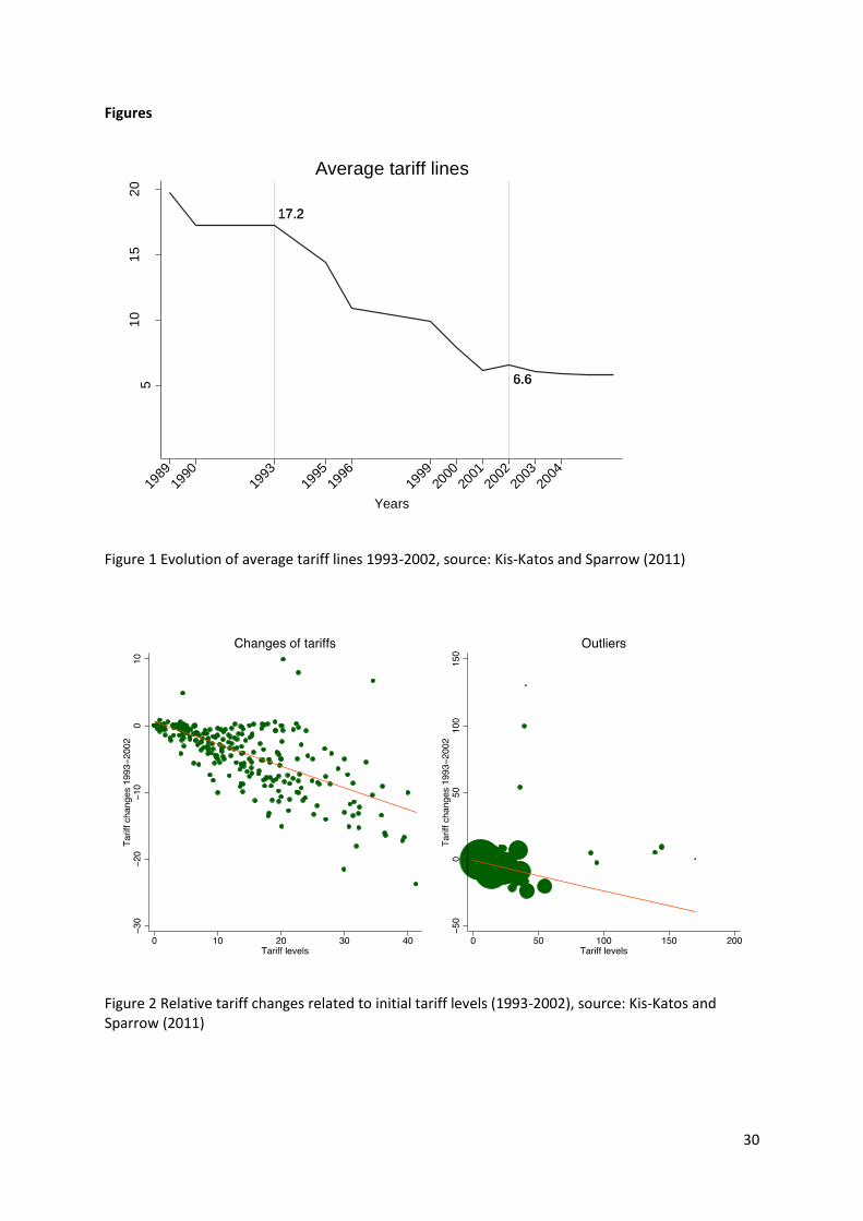
Figure 1 shows the reduction in average unweighted effectively applied tariff lines across the 1990s:

on average, tariff lines reduced from 17.2% in 1993 to 6.6% in 2002. Tariff reductions were the

largest preceding the formation of the WTO but a second substantial wave of tariff reductions

followed in the post monetary crisis period as part of the IMF conditionality package, starting with

1999. Table 1 shows the detailed evolution of the tariff schedule for 20 major tradable sectors,

which are defined according to a concordance of tariff information and census labour market data.

These tariff reductions happened across the board and were the highest in those industries that

started with the highest original tariff levels, due to the prevalence of firm-specific protection

measures in Indonesia (Basri and Hill 1996). In particular, some manufacturing sectors (such as

wood, textiles or other manufacturing) with high initial average levels of protection saw average

tariff rates reduce to below 10% by 2002. The food sector is an exception (with an average tariff of

12.6% in 2002), partly because of tariffication and later exemption of alcoholic beverages.

The period before the economic crisis was also characterised by high labour market flexibility and a

highly elastic supply of unskilled labour (Manning 2000). The early 1990s saw a continued shift from

agricultural towards urban employment, an expanding service sector and the growth of an export-

oriented economy. These structural changes were accompanied by steadily decreasing poverty

rates. Suryahadi, Suryadarma and Sumarto (2009) argue that the growth in urban services was a

powerful driving force behind these poverty reductions. Increases in inequality during this period

suggest, however, that the beneficial effects of the reforms were not concentrated on the very poor

(Miranti 2010). At the same time, labour regulation started to tighten somewhat, with rising

minimum wages and extensions of social security coverage.

The 1997/98 crisis had its roots in a monetary contagion leading to a large outflow of foreign capital,

currency depreciation, as well as short-term agricultural price hikes. This also led to a sudden

increase in expenditure poverty and a temporary restructuring of the labour force towards

subsistence production in agriculture. The crisis’ impacts were geographically clustered (Java being

most strongly hit), but did not differ considerably between rural and urban regions or by the initial

levels of poverty (Wetterberg, Sumarto and Pritchett 2001). The extent of expenditure poverty

peaked around November of 1998 and declined sharply afterwards, with a quick recovery in

consumption growth (Suryahadi, Sumarto and Pritchett 2003).

4. Methods

Following Topalova (2010), several recent studies identify regionally differential effects of trade

liberalization by distinguishing between different levels of regional exposure to trade based on the

8

pre-reform labour market structure of the region (Kovak 2010, McCaig 2011, Fukase 2013, Castilho

et al. 2012). The advantage of this method is that it does not only focus on the manufacturing sector

or formal employment but measures the effects of trade liberalization at the household level. To

define tariff exposure, it uses the labour structure of local residents based on household surveys,

irrespectively of the specific place and geographic location of their work, and hence focuses on tariff

effects important for local residents. The main poverty measures are derived from household

expenditure surveys, which capture the overall extent of regional poverty and offer a superior

source for poverty analysis. We complement this household based information with data from firm

and labour market surveys in order to investigate the labour market mechanisms that are behind

these poverty effects.

4.1 Measuring tariff exposure at district level

Our empirical strategy applies a measure of district tariff exposure that combines variation over time

in nationally determined import tariffs with district specific labour shares in the initial pre-reform

period:

The tariff exposure measure of district k in year t, , is calculated as a weighted average of

sectoral import tariffs of each sector h. The weights are given by the relative share of the

employment of sector h ( in the total labour force of district k ( , measured at an

initial time period, in 1990.

This tariff exposure measure is implicitly affected by the size of the non-tradable sector as weights

are normalized by the size of the total labour force of the district, and not only by the labour force

employed in tradable sectors. This is in line with the main definition applied by McCaig (2011) but

deviates from the methods employed by Topalova (2010) or Kovak (2010). Topalova (2010)

instruments tariffs weighted by labour market shares that include nontradables with tariffs weighted

by labour market shares in tradable sectors only. Kovak (2010) argues that one should drop the

nontradables sector altogether since there should be a perfect pass-through effect from tradable

price changes to nontradable prices. However, the regional size of the nontradable sectors will

matter if the pass-through is imperfect. Under robustness checks in section 6.2 we address the

sensitivity of our results to the exclusion of the nontradable sectors from the weighting scheme.

9

In addition to our main tariff exposure based on the labour market structure, we also compute

regional tariff exposure measures weighted by the regional industrial structure. This enables us to

identify the effects of tariff changes on the wage bill and employment of regionally important firms.

These alternative tariff measures are based on the output structure of formalized firms with at least

20 employees (from SI, the industrial census). Following the insights of Amiti and Konings (2007) and

Amiti and Cameron (2012), we distinguish between tariffs on firm output and tariffs on the

intermediate inputs used by firms. While output tariffs can be expected to affect firm productivity

through increased competition on the output markets, lower input tariffs have a more direct

productivity enhancing role by rendering inputs cheaper (Amiti and Konings 2007). Input (but not

output) tariff reductions have also been shown to go along with reductions in industrial skill premia

(Amiti and Cameron 2012).

In our application, we redefine the product level tariff measures to once again capture regional

differences in tariff exposure:

The output tariff measure weights national tariffs in sector s at year t by the industry’s initial share in

region k’s industrial output, , as recorded in the industrial census in the initial year

1993.8

For computing the input tariff, we rely on a national input-output table from 1990 to generate a

measure of regional exposure to input tariffs based on the regional sectoral structure:

For this, we weight the tariff on each input good j in year t by the initial share of the j-th industry

among the inputs of any output sector s, We once again aggregate these input

tariff measures across all output producing industries of the region, which are then weighted by the

output industry’s initial relative regional importance, . Since our input-output data

does not vary across regions, we have to assume that the national structure of inputs adequately

describes the regional input structures, at least on average. By using a pre-reform input-output table

we can ensure that tariff induced shifts in the industrial structure are not reflected in the measure.

8 After taking tariff and input-output table concordances into account, we are able to distinguish between

S=60 different tradable output industries.

10

These tariff measures reflect the presence of nontradable goods to a different extent. The output

tariff is weighted by tradable goods only since all industrial products included in the weighting

scheme are tradable. The input tariff takes nontradable inputs into consideration implicitly, by

including nontradable goods in the total sectoral inputs .

4.2 Empirical specification and identification

The primary interest of our study lies in understanding how regional exposure to tariff reductions

affected regional levels of poverty. According to the neoclassical theory of comparative advantage,

reduction in trading costs in a labour abundant economy can be expected to increase specialization

in the production of unskilled labour intensive goods, which should lead to relative improvements in

the wages of the less skilled population. Hence, the poverty reducing effects of international trade

will be primarily transmitted through labour market mechanisms. In order to investigate these

mechanisms, we focus not only on poverty measures but also on labour market outcomes. More

specifically, we test whether tariff reductions affect sector mobility, labour market participation and

formalization, job creation and wages.

Our main estimating equation takes the following first difference specification:

,

where denotes the district level dependent variables (poverty rates, labour and formalization

shares, average or total wages and employment). is a vector of time variant control variables

(share of rural population, share of working population aged 16-60, adult (20+) literacy rates,

minimum wages). The vector of initial conditions, includes the 1990 labour shares in the region

that are used as tariff weights, aggregated to one digit sectors, the 1990 rural population shares,

and, in some specifications, the initial levels of the dependent variable. Time and island interaction

terms are included to control for regions specific time effects. The main islands are defined as

Java, Sumatra, Kalimantan, Sulawesi, while the remaining smaller islands are grouped together.

The difference specification addresses the potentially endogenous nature of the components in the

tariff exposure measure. First, the potential bias due to endogenous tariff setting at the national

level is eliminated by controlling for national variation over time and by considering only within-

district variation. Second, by taking first differences and removing district fixed effects, we purge any

bias due to unobserved heterogeneity that might be introduced by the initial district sectoral

structure in employment and industry output. Moreover, the district labour and industry output

11

shares by sector are taken at 1990 values and are therefore not directly influenced by district

poverty profiles and labour market developments in 1993.

This approach relies on the indentifying assumption that there are no unobserved time variant

confounders. This assumption will be violated if poverty trends and labour market dynamics are

related to the initial sectoral composition of district economies. The most relevant potential

confounding trends include structural change, overall economic development and social policies.

Structural change involves a gradual shift from agriculture to manufacturing and service sectors. The

extent and speed of such structural change may vary by the initial size of the agricultural sector and

the share of the population living in rural areas. Changes in poverty incidence will also be driven by

overall economic development as well as targeted social policies. These may vary by initial levels of

poverty (due to convergence or policy targeting) and by local economic structure.

We deal with these potential confounding trends by adding controls for initial conditions: initial

sectoral labour shares (measured at the one-digit level) as well as the share of rural population in

1990. As an additional sensitivity check we include the 1993 value of the dependent variables (P0, P1

and P2) to proxy for convergence and targeting. Finally, we conduct placebo tests. If confounding

trends are driving our results, through initial labour shares, then we would expect that current

poverty changes are correlated with future changes in local tariff exposure. The placebo tests consist

of regressions of poverty changes, , on changes in tariff exposure of the following period,

, where the null of no confounding trends is rejected if the tariff coefficient is

statistically significant.

The 1997/98 financial crisis poses a potential problem for our empirical strategy. Although our

observation period only includes pre- and post-crisis years (1996 and 1999), the post-crisis recovery

remains a potentially confounding effect. We deal with this concern in two ways: we include in all

regressions island-year fixed effects that distinguish between five main geographic units and allow

the crisis effects to vary across the regions. Given the empirical evidence on the strong geographical

clustering of the poverty effects of the crisis (Wetterberg, Sumarto and Pritchett 2001), we are able

to capture a part of the crisis effects already through this strategy. Additionally, we also re-estimate

our models for separate, shorter time periods, pre-crisis (1993-1996) and for the post-crisis period

(1999-2002).

12

5. Results

5.1 Poverty

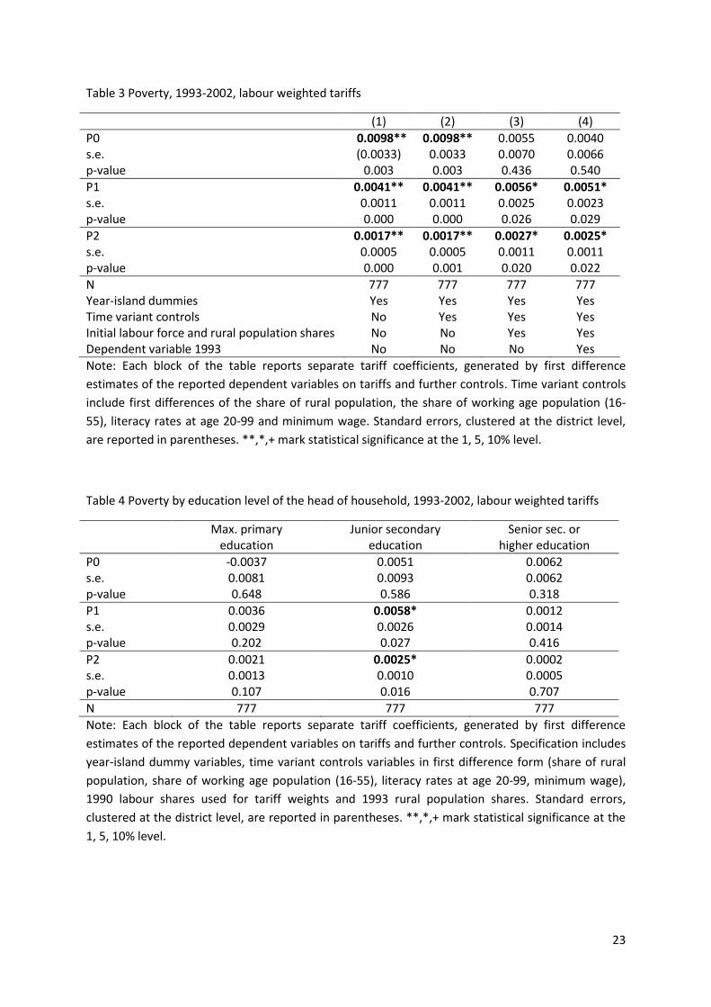
The general effects of tariff reductions on our three poverty measures (P0, P1 and P2) for different

specifications are shown in Table 3. There is a positive correlation between the poverty head count

and tariff exposure, implying that tariff reduction is associated with a reduction in poverty. This

relationship also holds after controlling for year-island fixed effects and time variant controls.

However, once we control for initial conditions (labour force structure and rural population size), the

coefficient reduces by half and is no longer statistically significant.

For both the poverty gap and poverty severity, on the other hand, the estimates are robust to

including initial conditions. Tariff reductions seem to have contributed to alleviating the depth of

poverty in Indonesia and have been particularly favourable for the very poor. A percentage point

reduction in tariff exposure is associated with a decrease of the poverty gap equivalent to 0.6

percent of the poverty line, and a decrease of poverty severity by 0.003.

Column (4) in Table 3 presents a specification where we control for initial levels of the dependent

variable, to assess whether initial poverty is associated with differential parallel trends that may

confound our estimates. We find no evidence of this, as the results are robust to including these

variables. Since we prefer not to include lagged levels of the dependent variable in a fixed effects

specification, we omit these in the remainder of the analysis.

Table 4 disaggregates the results from our preferred specification (column 3 in Table 3) by skill level

of the household head. We distinguish between three educational categories: household heads with

at most primary education, those with completed junior secondary education, and those with at

least a completed senior secondary education. The reductions in poverty depth and severity seem to

be driven by low- and medium skilled labour, although the estimates for the share of population

where the household head has at most primary education is not as precise as those for the middle-

skilled. For the high skilled population the estimates are small and not statistically significant,

presumably partly due to the relatively lower incidence of poverty in this group.

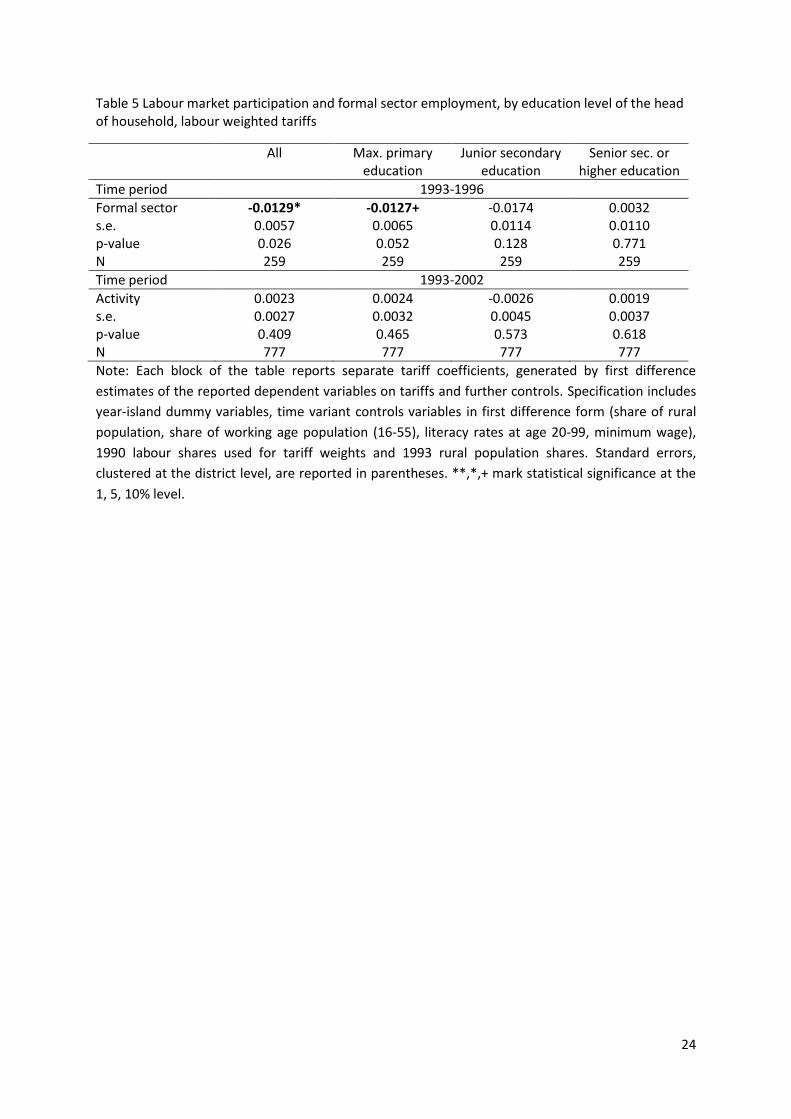
5.2 Labour market dynamics

As documented in Table 5, tariff reduction is associated with increased formal sector employment,

which measures the share of the active population employed either by the government, a private

sector employer or an employer who has permanent workers. This effect is driven by an increasing

formalization of the labour force among low and middle skilled workers whereas there is no similar

13

effect among higher skill workers.9 As formal sector jobs are usually generating larger and less

volatile (more secure) incomes, job formalization could have considerably contributed to the

favourable poverty effects of trade liberalization. By contrast, we find no notable effects on labour

market activity, which suggests that income effects from trade liberalization have been induced

mainly through job creation in the formal sector, and low skilled labour moving from informal to

formal sector jobs.

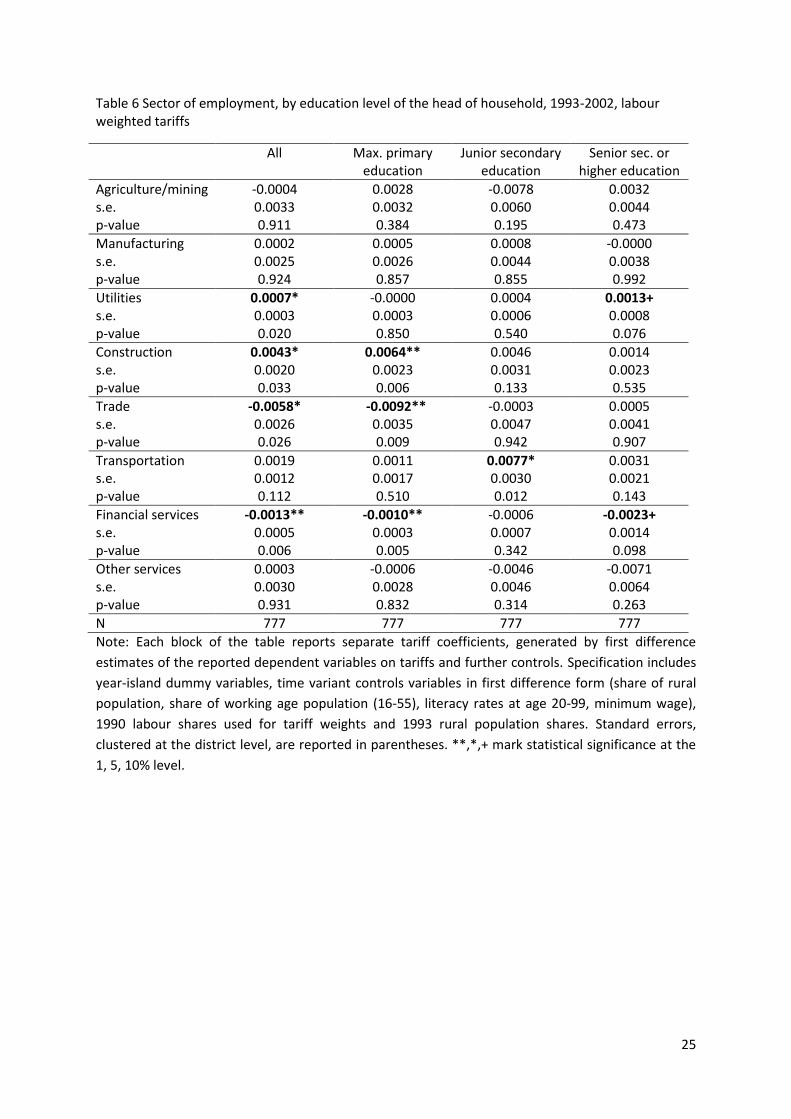
Table 6 presents the effects of exposure to trade liberalization on the regional distribution of the

broad sector of employment. Tariff reductions do not seem to have lead to much mobility between

tradable and non-tradable sectors, at least in aggregate terms. We find no evidence that changes in

the share of workers employed in agriculture, mining, and manufacturing could be explained by

trade liberalization. This is despite the fact that mobility between sectors in the study period was

high (Suryahadi 2003). The above result however does not preclude the possibility of finer-scale

migration across different parts of these more broadly defined sectors. Moreover, we see some

evidence for reallocation of labour across the various nontradable sectors: among low skilled

workers tariff reduction has lead to decreasing labour shares in construction and increasing shares in

trade and financial services. We also see an increased share of financial services among the high

skilled workers, at the expense of the utilities sector.

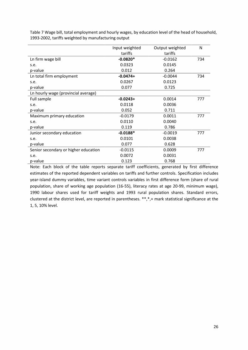
5.3 Firms: wages and workers

Previous studies document that trade liberalization in Indonesia has improved firm productivity

(Amiti and Konings 2007) and increased the relative magnitude of the wage bill paid by

manufacturing firms to lower as opposed to high skilled workers (Amiti and Cameron 2012). These

effects were in particular due to decreases in import tariffs on intermediate production goods used

by the firms. These findings suggest that direct improvements in the profitability of local firms might

also help explaining the observed favourable income effects to the poor. In order to investigate this

channel more closely, we extend the analysis to the total wage bill of large manufacturing firms in

the region and total employment by those firms. We use the same manufacturing firm data as the

two studies above and also differentiate between the effects of tariffs for intermediate inputs and

production outputs, but run the analysis at the level of the regional economies in order to retain

comparability with our previous results.

Table 7 shows that both the total manufacturing wage bill and total employment increase with a

decrease in tariffs on product groups that are relevant as input goods for the regional production: a

9 These estimates are available only for the time period 1993 to 1996 because we are not able to construct a

time consistent variable for formal labour due to changes in the Susenas questionnaire in both 1999 and 2002.

14

one percentage point reduction in input tariffs increases the average wage bill by 8.2 percent and

total employment by 4.7 percent.10 By contrast, we do not find evidence that reductions in tariffs

that are relevant to the structure of the regional economic output affect employment or the wage

bill. Together with the findings by Amiti and Cameron (2012), this seems to suggest that trade

liberalization has led to job creation in the formal manufacturing sector, in particular for low skilled

workers. Moreover, the total wage bill has increased relatively more strongly due to tariff reductions

than total employment, suggesting an average increase in wages or at least an increase in per capita

work intensity.

Since the SI data does not provide information on the hours worked, we cannot distinguish between

these two potential margins of adjustment. However, we can look at average wages at province

level, which are collected by the labour force survey (Sakernas). As the number of provinces is

considerably lower than the number of districts (23 as compared to 259), this is admittedly a much

cruder measure, but can be disaggregated by education level.

The province level estimates confirm that wages have increased as a result of tariff reductions for

intermediate inputs, while no significant effects could be observed from changes in output tariffs. A

one percentage point reduction in input tariffs reduced average hourly wages by 2.4 percent.

Moreover, the effects seem larger for relatively low skilled workers, although the estimates are

imprecise.

6. Sensitivity analysis and caveats

6.1 Robustness of poverty results to confounding trends and definitions of tariff measures

Our specifications address the issue of confounding trends in poverty that are related to the original

economic/labour market structure of the districts by controlling for initial labour shares of the main

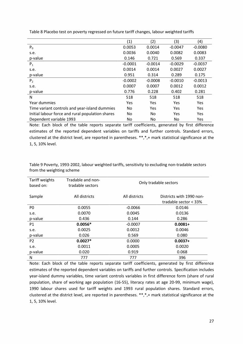
sectors as well as initial rural shares in the districts. In addition, Table 8 presents placebo test results

from regressions of current reductions in poverty on future reductions in our tariff measure (using a

one-period lead). Significant effects of future tariff changes on current outcomes would mean that

our results are still biased by confounding trends that drive poverty reduction and are imperfectly

controlled for by the initial conditions. We do not find any evidence for this problem: the future

tariff coefficients are small and not statistically significant, irrespective of the specification.11

10

In our sample, the input tariff measure decreased on average by 1.8 percentage points per period. 11

We also conduct placebo tests for a two-period lead, that is, we regress 1993-1996 poverty changes on 1999-2002 changes in tariff exposure. These tests provide similar results.

15

In our analysis we define the tariff measures based on the labour shares of the total regional

economy, including both traded and non-traded sectors. However, some studies propose a different

approach and argue that labour shares should be calculated only with respect to the size of the

tradable sectors (e.g. Topalova 2011, Kovak 2010).

Table 9 contrasts our results to those using the alternative weighting scheme. Column (1)

reproduces our previous results, column (2) shows poverty results based on tradable sector weights

only, whereas column (3) splits the sample and presents results based on tradable sector weights in

those districts where the labour force share of the non-tradable sector in 1990 was below the

median of 33%. These results show that the poverty effects of tariff reductions are driven by the

effects of trade liberalization in districts where the tradable sector is large enough such that poverty

effects can be measured with precision at district level. The tariff exposure measure that excludes

the non-tradable sector does not pick up any poverty effects, but when we focus only on the 50% of

districts with a relatively small non-tradable sector, we find results similar to those for the tariff

exposure that includes the non-tradable share. These results seem to suggest that the perfect pass-

through assumption holds only if the size of the tradable sector is sufficiently large.

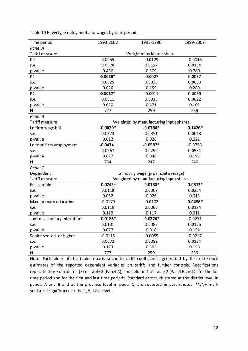
6.2 The monetary crisis and differential effects over time

The Southeast Asian monetary crisis of 1997/98 constitutes a potentially important confounding

factor during the analysed time period, especially since it has lead to a short-time spike in relative

food prices and sharp short-term increases in poverty. Since the effects of the crisis were strongly

geographically clustered, the inclusion of island-year fixed effects deals partly with this problem.

However, in order to exclude that the crisis confounds our estimates, we repeat our main

specifications, excluding the crisis years, for the pre-crisis and post-crisis periods separately.

Table 10 show the results by time period. The estimates for the poverty gap and poverty severity are

consistent for the 1999-2002 period but not precise, presumably due to the smaller sample size.

However, we find no evidence for the 1993-1996 period. Tariff reductions increased total wages paid

by manufacturing firms during both periods, but the effect is twice as strong in 1999-2002 as in

1993-1996. However, we only see an increase in total firm employment in 1993-1996. The results for

province average hourly wages suggest that these effects also translated into higher wages,

especially after the crisis. Moreover, the post-crisis wage increase was especially strong for low

skilled workers, while pre-crisis effects on wages were mainly observed for workers with junior

secondary schooling. These results are consistent with the findings for poverty outcomes: while tariff

16

reductions seem to have affected household incomes through wage increases and job creation, the

poorest segments of the population benefitted especially in the post crisis period.

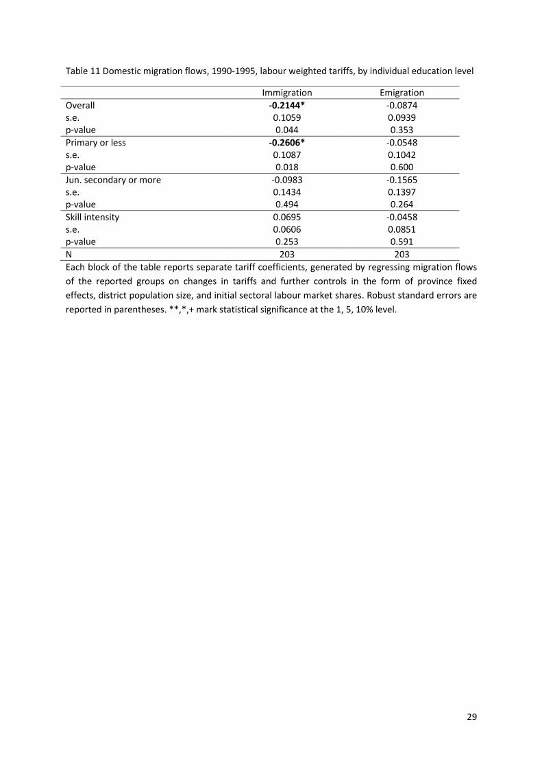
6.3 Migration

Migration can offer a further channel of transmission for the effects of trade liberalization by

measuring the extent of regional reallocation of labour; at the same time it can also confound our

poverty estimates over time. In order to test for a correlation between tariff reductions and

migration, Table 11 relates across-district migration between 1990 and 1995 to changes in district

tariff exposure over the same time period. We focus on the first part of our period of analysis since

migration flows preceding 2000 were strongly affected by the economic crisis as well as high-

intensity conflict.12 The available data do not allow us to identify causal effects of tariff reductions on

internal migration. Nevertheless, we do find descriptive evidence that the direction of internal

migration flows is towards districts with relatively strong exposure to tariff reductions, controlling

for province fixed effects (for 25 provinces), district population size and labour shares by sector.

The results show no considerable association between regional exposure to tariff reductions and

emigration from the district for the period of 1990-1995. That is, we do not find evidence for

displacement effects due to structural change leading to out-migration of workers. At the same time

there is a statistically significant negative relationship between changes in tariff exposure and

immigration, especially for lower skilled workers. Thus, if anything, exposure to trade liberalization

has acted as a pull factor for migration. One possible explanation behind this effect is the creation of

new low skilled jobs that lead to increased immigration of low wage workers. These results also

imply that we might underestimate the extent of poverty reducing effects of trade, since it is

especially lower skilled and hence more likely poor workers who migrate into the regions more

affected by structural change. These migration inducing effects of tariff changes are in line with the

overall findings of McCaig (2011) on Vietnamese migration following the bilateral trade agreement

with the US, although unlike in Indonesia, in Vietnam migration increased for all skill categories, with

somewhat higher effects on the higher skilled.

7. Conclusion

We have examined the effects of trade liberalization in Indonesia from 1993 to 2002 on poverty

levels in 259 Indonesian districts and the role of labour market as channel for these effects. During

this period, Indonesia reduced its tariff barriers across all tradable sectors, with average import

12

Repeating the same regressions for the period of 1995 to 2000 shows no significant correlation between exposure to tariff reductions and cross-regional migration.

17

tariffs decreasing from 17.2 percent in 1993 to 6.6 percent in 2002. This period also saw a strong

reduction in poverty, despite a temporary setback from the 1997/1998 economic crisis.

The identification strategy relies on combining information on initial regional labour and product

market structure with the exogenous tariff reduction schedule over three-year intervals. The results

are robust to specification and controlling for initial conditions in labour market structure, and

placebo tests show no evidence that confounding trends are affecting the estimates.

Our results suggest that trade liberalization has contributed partially to poverty reduction in

Indonesia by increasing incomes for the poorest segment of the population. While we do not see

substantial effects on the poverty head count, we do find that tariff reductions led to a statistically

significant reduction of the depth and severity of poverty.

The driving mechanism behind these effects seems to be increasing firm competitiveness as a direct

result of reductions in import tariffs on intermediate goods; whereas we see no evidence of

displacement effects from increased foreign competition due to reductions in import tariffs on final

outputs. Increased firm competitiveness in turn induced a further formalization of the labour force,

job formation and wage increases for low- and medium skilled labour. These experiences with trade

liberalization add caution to the current policy debate in light of the recent surge in protectionist

tendencies in Indonesian trade and economic policies (Nehru 2013).

18

References

Amiti, M. and Cameron, L. (2012): Trade liberalization and the wage skill premium: Evidence from

Indonesia, Journal of International Economics, 87(2): 277–287.

Amiti, M. and Konings, J. (2007): Trade liberalization, intermediate inputs and productivity: Evidence

from Indonesia, American Economic Review, 97(5): 1611–1638.

Attanasio, O., Goldberg, P.K. and Pavcnik, N. (2004): Trade reforms and wage inequality in Colombia,

Journal of Development Economics, 74(2): 331–366.

Autor, D.H., Dorn, D. and Hanson, G.H. (2012): The China syndrome: Local labor market effects of

import competition in the United States, NBER Working Papers, No. 18054, National Bureau of

Economic Research, Inc., Cambridge, Mass.

Basri, M.C. and Hill, H. (1996): The political economy of manufacturing protection in LDCs: An

Indonesian case study, Oxford Development Studies, 24(3): 241–259.

Castilho, M., Menéndez, M. and Sztulman, A. (2012): Trade liberalization, inequality, and poverty in

Brazilian states, World Development, 40(4): 821–835.

Chiquiar, D. (2008): Globalization, regional wage differentials and the Stolper-Samuelson Theorem:

Evidence from Mexico, Journal of International Economics, 74(1): 70–93.

Fitrani, Hofman and Kaiser (2005): Unity in diversity? The creation of new local governments in de

decentralizing Indonesia, Bulletin of Indonesian Economic Studies 41(1): 57-79.

Fukase, E. (2013): Export liberalization, job creation, and the skill premium: Evidence from the US-

Vietnam Bilateral Trade Agreement (BTA), World Development, 41(C): 317–337.

Galiani, S. and Sanguinetti, P. (2003): The impact of trade liberalization on wage inequality: Evidence

from Argentina, Journal of Development Economics, 72(2): 497–513.

Goldberg, P.K. and Pavcnik, N. (2003): The response of the informal sector to trade liberalization,

Journal of Development Economics, 72(2): 463–496.

Goldberg, P.K. and Pavcnik, N. (2007): Distributional effects of globalization in developing countries,

Journal of Economic Literature, 45(1): 39–82.

Gonzaga, G., Menezes Filho, N. and Terra, C. (2006): Trade liberalization and the evolution of skill

earnings differentials in Brazil, Journal of International Economics, 68(2): 345–367.

Iacovone, L., Rauch, F. and Winters, L.A. (2013): Trade as an engine of creative destruction: Mexican

experience with Chinese competition, Journal of International Economics, 89(2): 379–392.

19

Kis-Katos, K. and Sparrow, R. (2011): Child labor and trade liberalization in Indonesia, Journal of

Human Resources, 46(4): 722–749.

Kovak, B.K. (2010): Regional labor market effects of trade policy: Evidence from Brazilian

liberalization, RSIE Discussion Papers No. 606, Research Seminar in International Economics,

University of Michigan, Ann Arbor, Michigan.

Manning, C. (2010): Labour market adjustment to Indonesia’s economic crisis: Context, trends and

implications, Bulletin of Indonesian Economic Studies, 36(1): 105–136.

McCaig, B. (2011): Exporting out of poverty: Provincial poverty in Vietnam and U.S. market access,

Journal of International Economics, 85(1): 102–113.

Minnesota Population Center (2011): Integrated Public Use Microdata Series, International: Version

6.1 (Machine-readable database). Minneapolis: University of Minnesota.

Miranti, R. (2010): Poverty in Indonesia 1984–2002: The impact of growth and changes in inequality,

Bulletin of Indonesian Economic Studies, 46(1): 79-97.

Nehru V. (2013): Survey of recent developments, Bulletin of Indonesian Economic Studies, 49(2):139-

166.

Porto, G.G. (2006): Using survey data to assess the distributional effects of trade policy, Journal of

International Economics, 70(1): 140–160.

Robertson, R., Sitalaksmi, S., Ismalina, P. and Fitrady, A. (2009): Globalization and working

conditions: Evidence from Indonesia. In Robertson, R., Brown, D., Gaelle, P and Sanchez-Puerta, M.-

L. (eds.): Globalization, wages, and the quality of jobs: Five country studies. Washington D.C.: World

Bank: 203–236.

Stolper, W.F. and Samuelson, P.A. (1941): Protection and real wages, Review of Economic Studies,

9(1): 58–73.

Suryahadi, A. (2003): International economic integration and labor markets: The case of Indonesia, In

Hasan, R. and Mitra, D. (eds.): The impact of trade on labor: Issues, perspectives, and experiences

from developing Asia, Amsterdam: Elsevier Science.

Suryahadi, A., Sumarto, S. and Pritchett, L. (2003): Evolution of poverty during the crisis in Indonesia,

Asian Economic Journal, 17(3): 221–241.

Suryahadi, A., Suryadarma, D. and Sumarto, S. (2009): The effects of location and sectoral

components of economic growth on poverty: Evidence from Indonesia, Journal of Development

Economics, 89(1): 109–117.

20

Topalova, P. (2010): Factor immobility and regional impacts of trade liberalization: Evidence on

Poverty from India, American Economic Journal: Applied Economics, 2(4): 1–41.

Wetterberg, A., Sumarto, S. and Pritchett, L. (1999): A national snapshot of the social impact of

Indonesia's crisis, Bulletin of Indonesian Economic Studies, 35(3): 145–152.

Winters, L.A., McCulloch, N. and McKay, A. (2004): Trade liberalization and poverty: The evidence so

far, Journal of Economic Literature, 42(1): 72–115.

WTO (1998): Trade Policy Review Indonesia, World Trade Organization, Geneva.

WTO (2001): Doha Ministerial Declaration, 4th session of the Ministerial Conference, World Trade

Organization, Geneva, Available online at http://www.wto.org/english/thewto_e/minist_e/

min01_e/mindecl_e.htm.

21

Tables

Table 1 Descriptive statistics

Variables Mean SD Min Max No. obs. Dependent var. P0 0.2723 0.1736 0 0.8726 1036 P1 0.0568 0.0494 0 0.3403 1036 P2 0.0177 0.0194 0 0.1555 1036 Formal sector 0.2955 0.1533 0.0407 0.6893 777 Activity 0.5830 0.0739 0.4094 0.8191 1036 Agriculture/mining 0.4948 0.2522 0.0037 0.9074 1036 Manufacturing 0.0983 0.0766 0.0023 0.5525 1036 Utilities 0.0032 0.0037 0 0.0218 1036 Construction 0.0393 0.0242 0.0007 0.1877 1036 Trade 0.1736 0.0913 0.0138 0.4670 1036 Transportation 0.0421 0.0272 0.0016 0.1520 1036 Financial services 0.0065 0.0088 0 0.0786 1036 Other services 0.1422 0.0856 0.0248 0.4990 1036 ln Firm wage bill 15.9102 2.4354 8.7806 22.1963 991 ln Total firm employment 7.9432 2.0552 2.9957 12.9947 991 ln Hourly wage 7.0960 0.4872 5.5213 8.1542 1036 ln Immigration 9.9146 0.9964 7.3914 12.6431 203 Skill intensity immigration 0.5396 0.3023 0.0368 2.6044 203 ln Emigration 10.1127 0.8617 7.5470 12.5040 203 Skill intensity emigration 0.6114 0.3568 0.0876 1.9583 203 Explanatory var. Labour weighted tariffs 6.1859 3.4828 0.3095 17.8596 1036 Manuf. output weighted tariffs 14.5944 6.8459 0 47.1813 1036 Manuf. input weighted tariffs 7.3058 3.5427 0 28.6421 1036 Labour w. tariffs (w/o nontraded) 12.2083 4.9927 3.5145 27.6609 1036 Rural share 0.6421 0.3166 0 1 1036 Share of aged 16 to 60 0.6493 0.0416 0.5183 0.8137 1036 Adult literacy rate (>20) 0.8443 0.1071 0.3122 0.9988 1036 Minimum wage 17.3567 11.1523 4.80 59.13 1036 Initial share of agric. workers 0.4977 0.2575 0 0.9377 1036 Initial share of mining workers 0.0126 0.0230 0 0.2169 1036 Initial share of manuf. workers 0.0996 0.07832 0 0.4410 1036

22

Table 2 Evolution of average effectively applied tariff rates by sector

1993 1996 1999 2002 Agriculture Plants and animals 17.1 12.0 10.3 4.8 Forestry 7.7 3.9 3.5 3.8 Hunting 5.3 4.3 2.2 2.7 Sea fishery 24.9 16.6 14.0 5.2 Fresh-water fishery 10.0 0.0 0.0 0.0 Mining Coal mining 5.0 5.0 5.0 5.0 Metal ores mining 3.3 3.2 3.5 2.8 Stones and sand mining 7.0 5.6 3.6 3.5 Salt mining 20.0 15.0 15.0 7.4 Minerals and chemicals mining 2.9 3.0 3.0 2.7 Other mining 4.0 3.4 3.6 3.6 Manufacturing Food, beverages, tobacco 23.4 18.1 17.1 12.6 Textiles, apparel, leather 26.0 20.1 16.5 9.4 Wood and products 30.0 16.6 14.1 7.7 Paper and products 20.2 9.5 8.1 4.8 Chemicals and products 11.9 9.4 8.7 6.1 Non-metallic mineral products 20.4 9.5 7.0 5.6 Basic metals 10.3 8.0 7.6 6.4 Metal products 15.8 8.1 7.9 4.9 Other manufacturing 32.0 18.9 18.4 9.6

Note: Sectors are defined based on a concordance between tariff and census labour market data.

Source: UNCTAD-TRAINS database.

23

Table 3 Poverty, 1993-2002, labour weighted tariffs

(1) (2) (3) (4)

P0 0.0098** 0.0098** 0.0055 0.0040 s.e. (0.0033) 0.0033 0.0070 0.0066 p-value 0.003 0.003 0.436 0.540

P1 0.0041** 0.0041** 0.0056* 0.0051* s.e. 0.0011 0.0011 0.0025 0.0023 p-value 0.000 0.000 0.026 0.029

P2 0.0017** 0.0017** 0.0027* 0.0025* s.e. 0.0005 0.0005 0.0011 0.0011 p-value 0.000 0.001 0.020 0.022

N 777 777 777 777 Year-island dummies Yes Yes Yes Yes Time variant controls No Yes Yes Yes Initial labour force and rural population shares No No Yes Yes Dependent variable 1993 No No No Yes

Note: Each block of the table reports separate tariff coefficients, generated by first difference

estimates of the reported dependent variables on tariffs and further controls. Time variant controls

include first differences of the share of rural population, the share of working age population (16-

55), literacy rates at age 20-99 and minimum wage. Standard errors, clustered at the district level,

are reported in parentheses. **,*,+ mark statistical significance at the 1, 5, 10% level.

Table 4 Poverty by education level of the head of household, 1993-2002, labour weighted tariffs

Max. primary education

Junior secondary education

Senior sec. or higher education

P0 -0.0037 0.0051 0.0062 s.e. 0.0081 0.0093 0.0062 p-value 0.648 0.586 0.318

P1 0.0036 0.0058* 0.0012 s.e. 0.0029 0.0026 0.0014 p-value 0.202 0.027 0.416

P2 0.0021 0.0025* 0.0002 s.e. 0.0013 0.0010 0.0005 p-value 0.107 0.016 0.707

N 777 777 777


estimates of the reported dependent variables on tariffs and further controls. Specification includes

year-island dummy variables, time variant controls variables in first difference form (share of rural

population, share of working age population (16-55), literacy rates at age 20-99, minimum wage),

1990 labour shares used for tariff weights and 1993 rural population shares. Standard errors,

clustered at the district level, are reported in parentheses. **,*,+ mark statistical significance at the

1, 5, 10% level.

24

Table 5 Labour market participation and formal sector employment, by education level of the head of household, labour weighted tariffs

All Max. primary education



Time period 1993-1996

Formal sector -0.0129* -0.0127+ -0.0174 0.0032 s.e. 0.0057 0.0065 0.0114 0.0110 p-value 0.026 0.052 0.128 0.771 N 259 259 259 259

Time period 1993-2002

Activity 0.0023 0.0024 -0.0026 0.0019 s.e. 0.0027 0.0032 0.0045 0.0037 p-value 0.409 0.465 0.573 0.618 N 777 777 777 777







1, 5, 10% level.

25

Table 6 Sector of employment, by education level of the head of household, 1993-2002, labour weighted tariffs

All Max. primary education



Agriculture/mining -0.0004 0.0028 -0.0078 0.0032 s.e. 0.0033 0.0032 0.0060 0.0044 p-value 0.911 0.384 0.195 0.473

Manufacturing 0.0002 0.0005 0.0008 -0.0000 s.e. 0.0025 0.0026 0.0044 0.0038 p-value 0.924 0.857 0.855 0.992

Utilities 0.0007* -0.0000 0.0004 0.0013+ s.e. 0.0003 0.0003 0.0006 0.0008 p-value 0.020 0.850 0.540 0.076

Construction 0.0043* 0.0064** 0.0046 0.0014 s.e. 0.0020 0.0023 0.0031 0.0023 p-value 0.033 0.006 0.133 0.535

Trade -0.0058* -0.0092** -0.0003 0.0005 s.e. 0.0026 0.0035 0.0047 0.0041 p-value 0.026 0.009 0.942 0.907

Transportation 0.0019 0.0011 0.0077* 0.0031 s.e. 0.0012 0.0017 0.0030 0.0021 p-value 0.112 0.510 0.012 0.143

Financial services -0.0013** -0.0010** -0.0006 -0.0023+ s.e. 0.0005 0.0003 0.0007 0.0014 p-value 0.006 0.005 0.342 0.098

Other services 0.0003 -0.0006 -0.0046 -0.0071 s.e. 0.0030 0.0028 0.0046 0.0064 p-value 0.931 0.832 0.314 0.263

N 777 777 777 777







1, 5, 10% level.

26

Table 7 Wage bill, total employment and hourly wages, by education level of the head of household, 1993-2002, tariffs weighted by manufacturing output

Input weighted tariffs

Output weighted tariffs

N

Ln firm wage bill -0.0820* -0.0162 734 s.e. 0.0323 0.0145 p-value 0.012 0.264

Ln total firm employment -0.0474+ -0.0044 734 s.e. 0.0267 0.0123 p-value 0.077 0.725

Ln hourly wage (provincial average)

Full sample -0.0243+ 0.0014 777 s.e. 0.0118 0.0036 p-value 0.052 0.711

Maximum primary education -0.0179 0.0011 777 s.e. 0.0110 0.0040 p-value 0.119 0.786

Junior secondary education -0.0188* -0.0019 777 s.e. 0.0101 0.0038 p-value 0.077 0.628

Senior secondary or higher education -0.0115 0.0009 777 s.e. 0.0072 0.0031 p-value 0.123 0.768







1, 5, 10% level.

27

Table 8 Placebo test on poverty regressed on future tariff changes, labour weighted tariffs

(1) (2) (3) (4)

P0 0.0053 0.0014 -0.0047 -0.0080 s.e. 0.0036 0.0040 0.0082 0.0083 p-value 0.146 0.721 0.569 0.337

P1 -0.0001 -0.0014 -0.0029 -0.0037 s.e. 0.0014 0.0014 0.0027 0.0027 p-value 0.951 0.314 0.289 0.175

P2 -0.0002 -0.0008 -0.0010 -0.0013 s.e. 0.0007 0.0007 0.0012 0.0012 p-value 0.776 0.228 0.402 0.281

N 518 518 518 518 Year dummies Yes Yes Yes Yes Time variant controls and year-island dummies No Yes Yes Yes Initial labour force and rural population shares No No Yes Yes Dependent variable 1993 No No No Yes


estimates of the reported dependent variables on tariffs and further controls. Standard errors,


1, 5, 10% level.

Table 9 Poverty, 1993-2002, labour weighted tariffs, sensitivity to excluding non-tradable sectors from the weighting scheme

Tariff weights based on:

Tradable and non-tradable sectors

Only tradable sectors

Sample All districts All districts Districts with 1990 non-

tradable sector < 33%

P0 0.0055 -0.0066 0.0146 s.e. 0.0070 0.0045 0.0136 p-value 0.436 0.144 0.286

P1 0.0056* -0.0007 0.0081+ s.e. 0.0025 0.0012 0.0046 p-value 0.026 0.569 0.080

P2 0.0027* 0.0000 0.0037+ s.e. 0.0011 0.0005 0.0020 p-value 0.020 0.919 0.068

N 777 777 396







1, 5, 10% level.

28

Table 10 Poverty, employment and wages by time period

Time period 1993-2002 1993-1996 1999-2002

Panel A Tariff measure Weighted by labour shares

P0 0.0055 -0.0129 -0.0046 s.e. 0.0070 0.0127 0.0164 p-value 0.436 0.309 0.780

P1 0.0056* -0.0027 0.0057 s.e. 0.0025 0.0036 0.0053 p-value 0.026 0.459 0.280

P2 0.0027* -0.0011 0.0036 s.e. 0.0011 0.0015 0.0022 p-value 0.020 0.471 0.102

N 777 259 259

Panel B Tariff measure Weighted by manufacturing input shares

Ln firm wage bill -0.0820* -0.0788* -0.1426* s.e. 0.0323 0.0351 0.0618 p-value 0.012 0.026 0.022

Ln total firm employment -0.0474+ -0.0587* -0.0758 s.e. 0.0267 0.0290 0.0581 p-value 0.077 0.044 0.193

N 734 247 240

Panel C Dependent Ln hourly wage (provincial average) Tariff measure Weighted by manufacturing input shares

Full sample -0.0243+ -0.0138* -0.0513* s.e. 0.0118 0.0062 0.0204 p-value 0.052 0.026 0.013

Max. primary education -0.0179 -0.0102 -0.0496* s.e. 0.0110 0.0065 0.0194 p-value 0.119 0.117 0.011

Junior secondary education -0.0188* -0.0220* -0.0251 s.e. 0.0101 0.0085 0.0176 p-value 0.077 0.010 0.154

Senior sec. ed. or higher -0.0115 -0.0055 -0.0217 s.e. 0.0072 0.0082 0.0154 p-value 0.123 0.505 0.158

N 777 259 259


estimates of the reported dependent variables on tariffs and further controls. Specifications

replicate those of column (3) of Table 3 (Panel A), and column 1 of Table 7 (Panel B and C) for the full

time period and for the first and last time periods. Standard errors, clustered at the district level in

panels A and B and at the province level in panel C, are reported in parentheses. **,*,+ mark

statistical significance at the 1, 5, 10% level.

29

Table 11 Domestic migration flows, 1990-1995, labour weighted tariffs, by individual education level

Immigration Emigration

Overall -0.2144* -0.0874 s.e. 0.1059 0.0939 p-value 0.044 0.353

Primary or less -0.2606* -0.0548 s.e. 0.1087 0.1042 p-value 0.018 0.600

Jun. secondary or more -0.0983 -0.1565 s.e. 0.1434 0.1397 p-value 0.494 0.264

Skill intensity 0.0695 -0.0458 s.e. 0.0606 0.0851 p-value 0.253 0.591

N 203 203

Each block of the table reports separate tariff coefficients, generated by regressing migration flows

of the reported groups on changes in tariffs and further controls in the form of province fixed

effects, district population size, and initial sectoral labour market shares. Robust standard errors are

reported in parentheses. **,*,+ mark statistical significance at the 1, 5, 10% level.

30

Figures

Figure 1 Evolution of average tariff lines 1993-2002, source: Kis-Katos and Sparrow (2011)

Figure 2 Relative tariff changes related to initial tariff levels (1993-2002), source: Kis-Katos and Sparrow (2011)

17.2

6.6

17.2

6.6

17.2

6.651

01

52

0

Effe

ctive a

pplie

d ta

riffs

1989

1990

1993

1995

1996

1999

2000

2001

2002

2003

2004

Years

Average tariff lines

31

Supplemental appendix

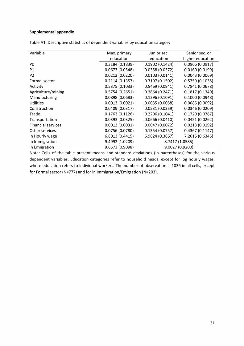
Table A1. Descriptive statistics of dependent variables by education category

Variable Max. primary education

Junior sec. education


P0 0.3184 (0.1839) 0.1902 (0.1424) 0.0966 (0.0917) P1 0.0673 (0.0548) 0.0358 (0.0372) 0.0160 (0.0199) P2 0.0212 (0.0220) 0.0103 (0.0141) 0.0043 (0.0069) Formal sector 0.2114 (0.1357) 0.3197 (0.1502) 0.5759 (0.1035) Activity 0.5375 (0.1033) 0.5469 (0.0941) 0.7841 (0.0678) Agriculture/mining 0.5754 (0.2651) 0.3864 (0.2471) 0.1817 (0.1349) Manufacturing 0.0898 (0.0683) 0.1296 (0.1091) 0.1000 (0.0948) Utilities 0.0013 (0.0021) 0.0035 (0.0058) 0.0085 (0.0092) Construction 0.0409 (0.0317) 0.0531 (0.0359) 0.0346 (0.0209) Trade 0.1763 (0.1126) 0.2206 (0.1041) 0.1720 (0.0787) Transportation 0.0393 (0.0325) 0.0666 (0.0410) 0.0451 (0.0262) Financial services 0.0013 (0.0031) 0.0047 (0.0072) 0.0213 (0.0192) Other services 0.0756 (0.0780) 0.1354 (0.0757) 0.4367 (0.1147) ln Hourly wage 6.8013 (0.4415) 6.9824 (0.3867) 7.2615 (0.6345) ln Immigration 9.4992 (1.0209) 8.7417 (1.0585) ln Emigration 9.6573 (0.9098) 9.0027 (0.9200)

Note: Cells of the table present means and standard deviations (in parentheses) for the various

dependent variables. Education categories refer to household heads, except for log hourly wages,

where education refers to individual workers. The number of observation is 1036 in all cells, except

for Formal sector (N=777) and for ln Immigration/Emigration (N=203).

32

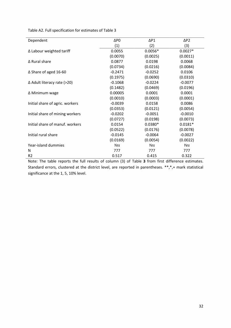
Table A2. Full specification for estimates of Table 3

Dependent ΔP0 ΔP1 ΔP2 (1) (2) (3)

Δ Labour weighted tariff 0.0055 0.0056* 0.0027* (0.0070) (0.0025) (0.0011) Δ Rural share 0.0877 0.0198 0.0068 (0.0734) (0.0216) (0.0084) Δ Share of aged 16-60 -0.2471 -0.0252 0.0106 (0.1975) (0.0690) (0.0310) Δ Adult literacy rate (>20) -0.1068 -0.0224 -0.0077 (0.1482) (0.0469) (0.0196) Δ Minimum wage 0.00005 0.0001 0.0001 (0.0010) (0.0003) (0.0001) Initial share of agric. workers -0.0039 0.0158 0.0086 (0.0353) (0.0121) (0.0054) Initial share of mining workers -0.0202 -0.0051 -0.0010 (0.0727) (0.0198) (0.0073) Initial share of manuf. workers 0.0154 0.0380* 0.0181* (0.0522) (0.0176) (0.0078) Initial rural share -0.0145 -0.0064 -0.0027 (0.0169) (0.0054) (0.0022) Year-island dummies Yes Yes Yes N 777 777 777 R2 0.517 0.415 0.322

Note: The table reports the full results of column (3) of Table 3 from first difference estimates.

Standard errors, clustered at the district level, are reported in parentheses. **,*,+ mark statistical

significance at the 1, 5, 10% level.

poverty, labour markets and trade liberalization in indonesiaftp.iza.org/dp7645.pdf · poverty,...

Documents