poverty, fertility preferences and family planning ... · poverty, fertility preferences and family...

For comments, suggestions or further inquiries please contact:

Philippine Institute for Development StudiesSurian sa mga Pag-aaral Pangkaunlaran ng Pilipinas

The PIDS Discussion Paper Seriesconstitutes studies that are preliminary andsubject to further revisions. They are be-ing circulated in a limited number of cop-ies only for purposes of soliciting com-ments and suggestions for further refine-ments. The studies under the Series areunedited and unreviewed.

The views and opinions expressedare those of the author(s) and do not neces-sarily reflect those of the Institute.

Not for quotation without permissionfrom the author(s) and the Institute.

September 2005

The Research Information Staff, Philippine Institute for Development Studies3rd Floor, NEDA sa Makati Building, 106 Amorsolo Street, Legaspi Village, Makati City, PhilippinesTel Nos: 8924059 and 8935705; Fax No: 8939589; E-mail: [email protected]

Or visit our website at http://www.pids.gov.ph

Aniceto C. Orbeta Jr.

DISCUSSION PAPER SERIES NO. 2005-22

Poverty, Fertility Preferencesand Family Planning Practice

in the Philippines

Poverty, Fertility Preferences and Family Planning Practice in the Philippines

Aniceto C. Orbeta, Jr. July 2005

Abstract This paper looks at the interaction of poverty, fertility preferences and family planning practice in the Philippines using the series of nationally representative Family Planning Surveys conducted annually since 1999 augmented by census and other survey data. Its contribution lies on providing recent and nationally representative empirical evidence on the long running but largely unresolved debate in the country on the relationship between fertility preferences and family planning and socioeconomic status. A detailed characterization of the relationships was done using cross tabulation analyses. In addition, and more importantly, a recursive qualitative response model was estimated to identify the determinants of fertility preferences and family planning practice across socioeconomic groupings. The paper show that while the number of children ever born is indeed larger among poorer households, their demand for additional children is lower and their contraceptive practice poorer. This result indicates that, in the case of the Philippines, the larger number of children among the poor is more the result of poorer contractive practice rather than higher demand. Keywords: Fertility Preferences, Family Planning, Socioeconomic Status,

Philippines

Poverty, Fertility Preferences and Family Planning Practice in the Philippines1

Aniceto C. Orbeta, Jr.2 July 2005

1. Introduction It is well known that poverty incidence is always higher among larger households. This is true in the Philippines as it is in many parts of the world. In the case of the Philippines, for instance, Orbeta (2005) highlights the enduring positive relationship between family size and the poverty incidence as well as severity using family income and expenditure data for the past 25 years. Results of research summarized in Orbeta (2005) also highlights how large family size creates the conditions for more poverty through its negative impact on household savings, labor force participation and earnings of parents as well as on the human capital investment in children. The flipside of this story is that its also well known that poorer households have poorer access to public services and access to family-planning services is not an exception. This is reflected in lower contraceptive prevalence rates and higher unmet need for family planning. The data also indicates that the desired family size is higher among the poor (Orbeta 2004a). Given that it is known that actual fertility is dependent on contraceptive practice, the question then is whether higher actual fertility among the poor is a result of higher demand or of poorer access to family planning or both. Clarifying these intertwined issues would help provide policy makers, wanting to reduce poverty among larger households, a clearer direction on what to do. This paper presents descriptive and multivariate analytical evidence on the relationship between poverty, fertility preferences and family planning practices using a recent nationally representative Family Planning Survey (FPS) in the Philippines. There are a few studies providing national survey and analytical evidence on this relationship and to the best knowledge of the author none using Philippine data. Previous analysis, e.g., DeGraff et al (1997), used sub-national surveys and did not deal directly with the role of different socioeconomic background which is the focus of this paper. Using cross-tabulation analyses utilizing a nationally representative survey data, the paper first characterizes these relationships. It then estimates the joint demand for additional children given children ever born and the use of modern contraception using a recursive discrete choice model that accounts for the correlations of the unobserved characteristics in these relationships. Like earlier studies (e.g., DeGraff et al 1997, Guilkey and Jayne, 1997) it recognizes the proper structuring of the variables, e.g. that children ever born is the product of past decision and that the demand for additional children is the more relevant current demand for children that affects the current demand 1 Paper presented at the 25th IUSSP International Population Conference, Tours, France, 18-23 July 2005, Session 163: Poverty, Households and Demographic Behavior. Attendance in the conference was with financial support from the French National Organizing Committee. 2 Correspondence: [email protected]. Senior Research Fellow, Philippine Institute for Development Studies. Part of this paper has been written while the author was Visiting Researcher at the Asian Development Bank Institute, Tokyo. Opinions expressed here are sole of the author and does not necessarily represent the position of the Philippine Institute for Development Studies or the Asian Development Bank Institute. Excellent research assistance by Janet Cuenca is gratefully acknowledged.

2

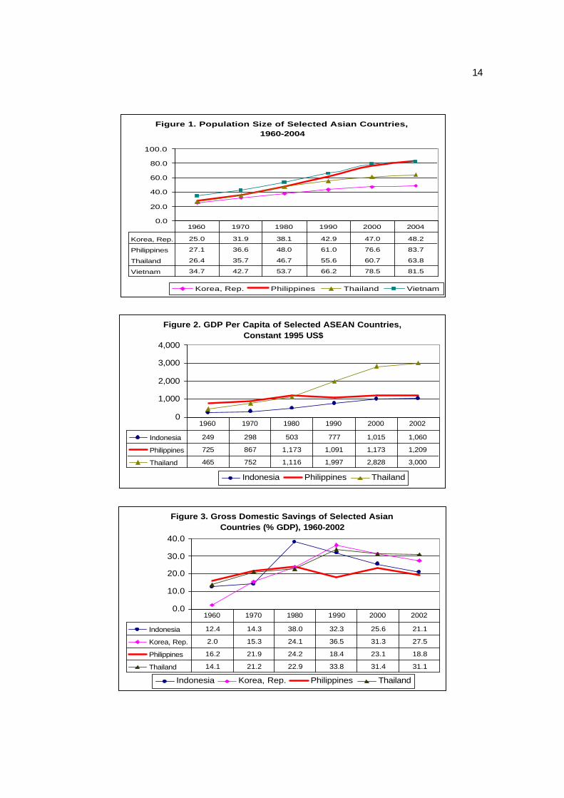
for contraception. Since the particular interest of the paper is in quantifying the role of socioeconomic status in these relationships, after controlling for other personal, household and community characteristics, a variable is provided to represent this particular concern. It uses a wealth index constructed from the presence of household amenities which the survey provides as a measure of the socioeconomic status of the household. The use of a wealth index was first introduced in Filmer and Pritchett (1998) and this has been used in many other studies. A complete description of the construction of the wealth index is provided in the Annex. The paper is organized as follows. The next section provides a brief overview of population and development relationships in the Philippines. This overview provides a brief background for the socioeconomic and demographic outcomes in the country. It also provides cross tabulation of relevant demographic outcomes by socioeconomic class. The cross-tabulation analysis is designed to provide the needed introduction to the multivariate analysis which follows in the third section of the paper. The last section summarizes and provides some implications of the results for policy. 2. Population and Development in the Philippine Context 2.1 Overview of population and development3 Around the beginning of 1960s, Philippines, Thailand and Korea have about the same population size. These two other countries have long achieved replacement fertility (total fertility rate (TFR) of around 2), Korea before the 1990s and Thailand about the middle of 1990, the Philippines has still a long way to go with a TFR of 3.5 as of 2003. As a result, the population sizes of these three countries have diverged. By around 2000, Philippines had about 30 million more people than Korea and 16 million more than Thailand (Figure 1). In addition, while these two countries continued to register consistent high growth, the Philippines had slow and inconsistent growth rates. After putting these two together, it would not be difficult to understand why the per capita income of the country has not gone far from 1,000 US dollars for more than two decades now (Figure 2). It would not be surprising also to know that poverty reduction has been slow and tentative (Reyes, 2002). As one looks at other development indicators, the overall long-term development picture given above is hardly surprising. Savings rates have been low, even often times lower than Indonesia in spite of the higher per capita income in the Philippines (Figure 3). Labor force participation of women is lower compared to many other countries in Asia even if the educational attainment of women is higher. The high school attendance rate 4 that the country is proud about for so long is eroding fast. Yet the issue of the role of population in development, in general and poverty and vulnerability, in particular, is largely unresolved. This reality persists despite the growing literature worldwide and also in the Philippines providing evidence on the importance of population growth and family size in development (see for instance Alonzo et al. (2004), Orbeta (2003) and de Dios and Associates (1993)). The two glaring proofs to this fact

3 This section draws heavily from Orbeta (2005). 4 That Philippines is an outlier in this regard is well-documented (see for instance, Berhman and Schneider, 1994; Behrman 1990)

3

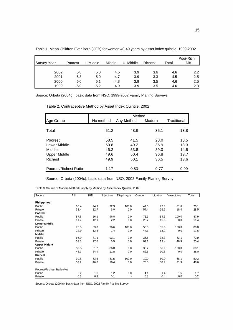
are: (a) the equivocal support given by the government to the population program, and (b) up to now virtually all of contraceptives supplies in public facilities are supplied by donors as national government has not appropriated money for these commodities5. Herrin (2002) describes in detail the stop-go attitude of government population policy. There are several ways the national leadership, both past and present, had avoided the issue. The current government, for instance, has left to local government units (LGUs) the provision of family planning services citing the Local Government Code (LGC) of 1991 as basis. The LGC has transferred many direct services, including maternal and child health service and family planning, to the LGUs. The lack of national guidance has resulted into fragmented and local programs often working in opposite directions largely depending on the persuasion of the local executive (Alonzo et. al 2004, Orbeta 2004b). One perhaps may ask whether there is any real demand for family planning services that government has to respond to. It should be mentioned that all demographic surveys showed the consistent high demand for family planning services from women of reproductive age (Herrin, 2002). Orbeta (2004a) also pointed out that the poor have lesser access to family planning services and that their wanted fertility is higher than those of the rich. The demand, therefore, for an appropriately funded population program is clear. What is absent is the national government’s resolve to push the program consistently as other countries, such as Thailand, Indonesia and Vietnam, have done. 2.2 Demographic Outcomes by Socioeconomic Class6 To provide a background for the multivariate analysis in the next section, this subsection present cross-tabulation of fertility and contraceptive practice by asset index quintile. Asset index quintiles were generated using the information on household amenities which are included in the FPS since the 1999 round following Filmer and Pritchett (1998). The full description of the construction of the asset index is described in the Annex. 2.2.1 Children Ever Born The main fertility variable that can be generated from the FPS is the Mean Children Ever Born (CEB)7. The CEB for women aged 40-49, who are considered to have completed or nearly completed fertility, is used as an indicator of fertility. Table 1 shows the CEB for women 40-49 by asset index quintile from 1999-2002. The mean CEB remained virtually constant over the years staying at around 4.6 per married woman. Also noteworthy is the stable difference in the mean CEB across socioeconomic classes. One finds that the difference in mean CEB for women 40-49 years old in the poorest and richest households is a little over 2 births. This difference hardly changed from 1999 to 2002. 5 USAID, the primary donor of contraceptive supplies, has recently indicated to government that it is phasing out its provision of contraceptive supplies. 6 This section draws heavily from Orbeta, A. (2004c). 7 The Total Fertility Rate (TFR) can be computed using the recorded births in the last three years asked in the FPS since 1996. The TFR computed, however, is too low and erratic in value compared to the ones generated from the National Demographic and Health Survey (NDHS), indicating perhaps, that the recording of bi rths is not as complete and as consistent. Perhaps this is because FPS does not have has elaborate probing and validating questions as the NDHS. See Orbeta (2004c) for the estimates.

4

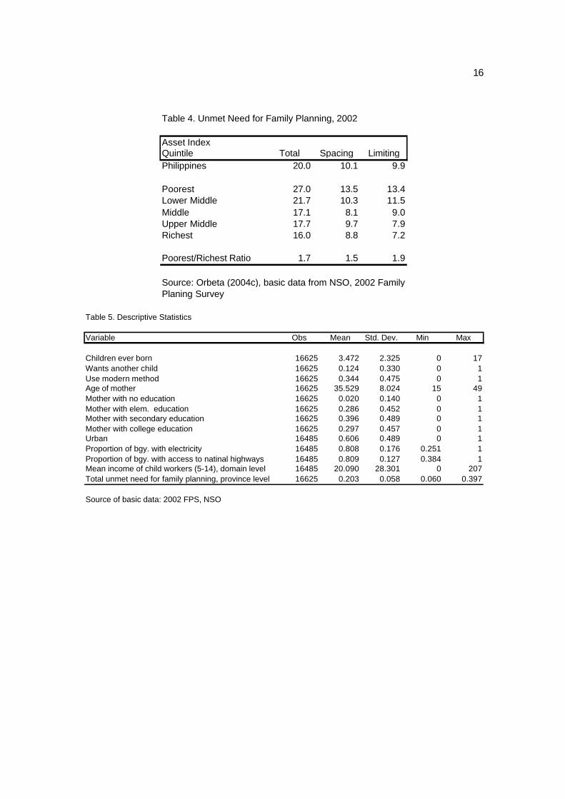
2.2.2 Contraceptive Prevalence The contraceptive prevalence of married women in 2002 is given in Table 2. It shows that a less than half of married women are using any contraception. A little over 70% of these women using some contraception are using modern methods. As pointed out in Orbeta (2004a), given the very slow rise in total contraception rates, the redeeming fact is that the proportion of women using modern methods is the only ones rising faster. As one looks across the socioeconomic classes, the main noticeable difference also lies in the use of modern methods. For the traditional method, there is virtually no difference between the richest and the poorest households. The difference for modern methods between the poorest and richest households, however, is above 8 percentage points. A lesser proportion of women from poorer households are using the modern methods. 2.2.3 Sources of Supply The proportion of women using public source is 70.1% while 28.5% is getting their supplies from private sources. All contraceptive supplies, except condoms, are sourced primarily from the public sector (Table 3). More than 80% of the poorest and as much as half of the women from the richest quintile source their supplies from the public sector. Only condoms and to some extent the pills and IUDs are sourced primarily from the private sector. 2.2.4 Unmet Need for Family Planning Table 4 shows that the unmet need for family planning is about 20% which is evenly distributed between spacing (10.1%) and limiting (9.9%) needs. Twenty seven percent of women from the poorest households indicated unmet need with 13.5% for spacing and 13.4% for limiting. Women from the richest households exhibited as 16% unmet need with 8.8% for spacing and 7.2% for limiting nearly one-half of the unmet need for the poor. Thus, the limiting need of women from the poorest household is almost twice as that for the women from the richest household while the spacing need is about one and half times more. 2.2.5 Demand for Children The FPS has no direct measure for the demand for children unlike the National Demographic and Health Survey (NDHS) which has a measure of wanted fertility. The latest NDHS done in 2003 indicates that difference between actual and wanted fertility among women from the poorest households is about 2 births. For women from the richest households, the difference between actual and wanted fertility, however, is less than half a birth. These figures have hardly changed based on the three NDHS rounds done between 1993 to 2003 (Orbeta 2004d).

5

3. Multivariate Analyses 3.1 Model To shed light on the differential impact of socioeconomic status on demographic behavior, the paper models the joint decision of contraception adoption and demand for additional children with an indicator of socioeconomic class as one of the explanatory variables after controlling for the usual individual, household and community characteristics. The paper estimates a model for the decision for using modern contraception and wanting an additional child given the number of children ever born. The model follows closely the model used in Degraff, Bilsborrow and Guilkey (1997). It assumes a sequential decision-making process rather than a full dynamic lifetime model which would require data at every stage of the decision processes that are not usually available. But unlike Degraff, Bilsborrow and Guilkey (1997) we did not assume location (community) fixed effects. The current problem modeled is the decision on whether or not to have an additional child and on the use of modern contraception. It is assumed that these decisions are correlated with past decisions embodied in the current number of children but in a recursive way. The current number of children is assumed to be the cumulative outcome of past decisions similar to Degraff, Bilsborrow and Guilkey (1997) and Guilkey and Jayne (1997). The impact of this outcome of past decisions is assumed to be only through its effect on the current demand for additional children. In turn, the current demand for additional children is expected to affect the decision to use modern contraception or not. Specifically the model estimated is the following

),,,(

),,,(

),,(

ccc

ddd

nnn

ZXdfc

ZXnfd

ZXfn

ε

ε

ε

=

=

=

The model presumes that the children ever born n is a function of a set of a common individual, household and community characteristics X, and other specific determinants to n, Zn . The demand for additional children d is a function of the children ever born, common characteristic X and determinants specific to d, Zd. Finally, the contraception c is a function of the demand for additional children, common characteristics X, and determinants specific to c, Zc. The error terms ε are by implication of the structure correlated. Similar models are in Bollen, Guilkey and Mroz (1995) and Guilkey and Jayne (1997). Bollen et al. (1997) uses the difference between the stated desired number of children and children ever born as the demand for children variable. In Guilkey and Jayne (1997) the demand for children is more finely disaggregated into wanted soon, wanted later, and wanted no more. In this paper, the demand for children is indicated by the response to the question on whether the woman wants another child.

6

In terms of contraception, Guilkey and Jayne (1997) used the finer disaggregation of modern, traditional and none. Degraff, Bilsborrow and Guilkey (1997) and Bollen, Guilkey and Mroz (1995), on the other hand, lumped modern and traditional together. In this paper, use of contraception is confined to the use of modern methods. This is influenced by the cross tabulation result that shows that the difference across socioeconomic classes is only evident in the use of modern methods. Given the structure of the model, the estimation strategy is as follows. The number of children model was estimated using OLS. This estimate was used as the first stage results in the demand for children equation. The demand for additional children and the use of modern contraception equations were also estimated using two types of two-stage probit estimation in addition to using ordinary probit estimates. This is because the number of children ever born is hypothesized to be endogenous in the demand for additional children equation while the demand for additional children is hypothesized to be endogenous in the demand for contraception equation. One is proposed in Lee (1981) that uses the predicted values of the endogenous variable and the other one is the one suggested in Rivers and Vuong (1988) which uses the actual values of the endogenous variable plus the estimated error from the first-stage regression as regressors in the second stage. While both produce consistent estimates, it has been argued (Rivers and Vuong 1988) that the latter generates asymptotically efficient estimates. It has been pointed out that the estimated errors using common statistical packages in the second stage regressions are biased and needs to be adjusted. Bollen, Guilkey and Mroz (1995), however, mentioned Monte Carlo experiments that show that the gains from adjusting the standard errors do not change substantially the resulting test results. Thus, no adjustment was done in the estimates in this paper. The predicted values of the children ever born variable or the estimated error term from this first stage run are used in the second stage estimation of the demand for additional children equation. In the case of the contraceptive use equation, the predicted values of the demand for additional children or the estimated error term from this first stage run was used in the second stage estimation. Finally, another way of dealing with the correlated error terms in the spirit similar to the seemingly unrelated regressions in linear models is using a bivariate probit model. This also provides a way for directly testing the correlation of the error terms of the two equations. This procedure was used to jointly estimate the demand for additional children and the contraception equation and provide corroborating evidence to the other estimation results. 3.2 Data Used The individual and household characteristics used in the estimation are from the nationally-representative 2002 Family Planning Survey (FPS). The survey is a rider to the April round of the quarterly Labor Force Survey (LFS). This survey has been conducted annually since 1995 except for years where the National Demographic and Health Survey (NDHS) are conducted. Like many surveys, the questions have evolved over the years. The 2002 FPS was chosen because it has the question needed to generate information on wanting a child in the future that are not available in the previous FPS besides the information on contraceptive use. These two questions are the dependent variable used in the literature to study the interaction between demand for children and demand for contraceptive use. The question on wanting an additional child is used to construct the current demand for children. The information on unwanted fertility was also used as an indicator of the availability of family planning services

7

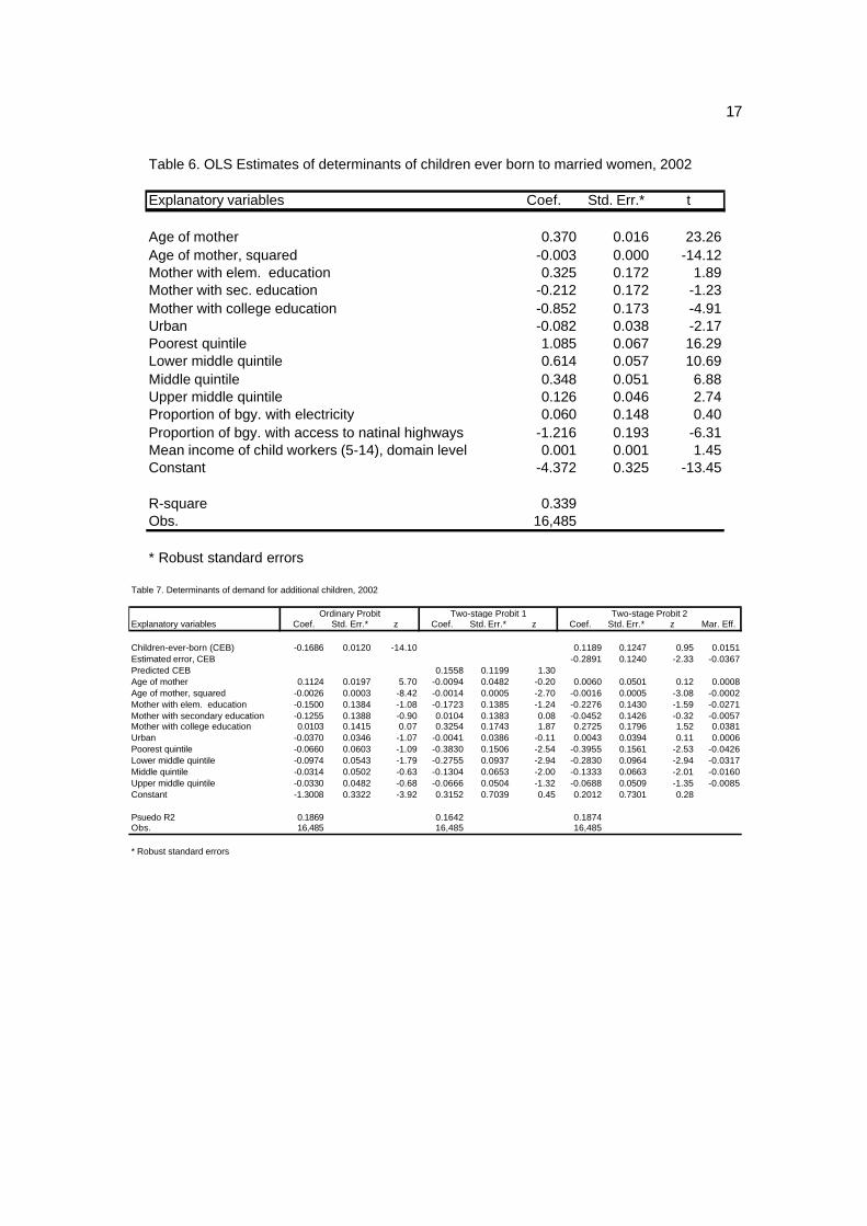
because there is no other family planning program information in this data set. It should be noted that Bruce (1990) considers information on unwanted fertility as the ultimate measure of the quality of family planning services. Finally, it has information on household amenities that can be used to construct an index for socioeconomic status whose role on the question of demand for children and contraceptive is the primary focus of the paper. This basic data set is augmented by community information taken from other sources. Community information such as the proportion of barangays with electricity and those with access to national highways are taken from the 2000 Census of Population and Housing. It is, therefore, assumed that not much has changed between the census and in 2002 particularly in the relative distribution of these types of infrastructure. The child wage variable which is an indicator of the economic services provided by children was generated from the Annual Poverty Indicators Survey (APIS) 2002. This represents the wage income for the past six-months, the reference period for the survey, of working children aged 5 to 14 years old. To control for inter-provincial price variations, the 2002 provincial price index from the NSO price division was used as a deflator. 3.3 Descriptive Statistics Table 5 shows the descriptive statistics of the variables used in the analysis. Only married8 women are considered in the analysis. The mean number of children ever born to respondent married women is less than 4 children although the number could be as high as 17. The proportion of married women who wanted another child is 12 percent. Thirty four percent of the married women are using modern methods. The average age is about 36 years. In terms of education, 29% had some elementary education, 40% had some secondary education, 30% had college education, and about 2% had no education. These proportions revealed the high educational attainment of Filipino women. The proportion living in urban areas is 49%. The proportion of barangays with electricity is about 81% and about the same proportion of barangays also has access to national highways. The six-month labor earnings of children 5-14 years old range from zero to 2079 or an average 20 pesos. Finally, the proportion of total (sum of limiting and spacing) unmet need for family planning is about 20%. 3.4 Estimation Results The estimation only includes married women of reproductive age and always employs robust standard error estimates. 3.4.1 Children Ever Born Table 6 shows the OLS estimates of the number of children ever born. The estimates confirm expectations that, controlling for the other variables, the children ever born for poorer households (wealth index quintiles 1 to 4) are all significantly bigger than for

8 This includes those living together. 9 This has been deflated using the consumer price index (1994=100). The recorded average six-month wage earnings of adults (15 years and above) is about 9,900.

8

women from the richest quintile, the omitted category. The poorest quintile, for instance, has an average of 1.1 children more than the richest. This is followed by the lower middle quintile with 0.6 more births and so on. The coefficients for the age of the mother show that, as expected, the number of children rises with age but at declining pace. The coefficients for the education dummy variables show that only the women with college education have significantly lower children ever born compared to the women with no education. Those with elementary and secondary education are not significantly different from those with no education. The impact of community variables confirms common expectations. Women living in urban areas have significantly lower children ever born. The results showed that the presence of electricity is not a significant determinant in contrast to earlier results such as Herrin (1979). Perhaps given the reach of electricity now compared to earlier periods, the availability of electricity no longer has pervasive effect as indicated in earlier studies. Access to national highways significantly lowers the number of children-ever-born confirming earlier results. The positive coefficient for the mean income of children workers lend some support to the hypothesis that children are desired because of their economic contribution to household income. However, this is not statistically significant implying perhaps that the influence in general is weak. It is worth noting that the recorded average contribution of children to household income is minuscule relative to the contribution of adult workers. 3.4.2 Demand for Additional Children Table 7 provides the results of the different estimation procedures employed for the demand for additional children. As mentioned earlier, the different estimation procedures are employed to consider the possible endogeneity of the children ever born variable in this equation. The impact of the number of children ever born on the demand for additional children has a mixed result. The ordinary probit estimate generated the expected negative sign and statistical significance but when in the two two-stage probit estimation was applied to allow for the endogeneity of this variable this coefficient become positive but insignificant. As argued in Rivers and Vuong (1988) the significance of the estimated error term in the two-stage probit 2 results confirms the endogeneity hypothesis making the ordinary probit estimate inconsistent. It also means that the depressing effect of the children ever born on the demand for additional children exhibited by the ordinary probit results cannot be relied upon particularly that the two-stage probit estimate yielded the opposite sign and not significant. Hence, we use the two-stage probit 2 results in subsequent discussions. The estimation results show that the demand for additional children rises with age but at declining rate. Education of the mother does not significantly affect the demand for additional children. There is no significant difference in demand for additional children between those living in the urban and rural areas. The impact of the wealth variable yielded interesting results. It shows that, except for the upper middle quintile, there is a significant negative difference in the demand for children between women from the lowest three wealth quintiles and the women from richest quintile households, the omitted category. This implies that given children ever born, it is not true that women from poorer households demand more children than those from the richer households, contrary to what many expect. The estimation result shows that they in fact demand less than the women from richer households with marginal effects that are increasing as one goes lower the wealth ladder.

9

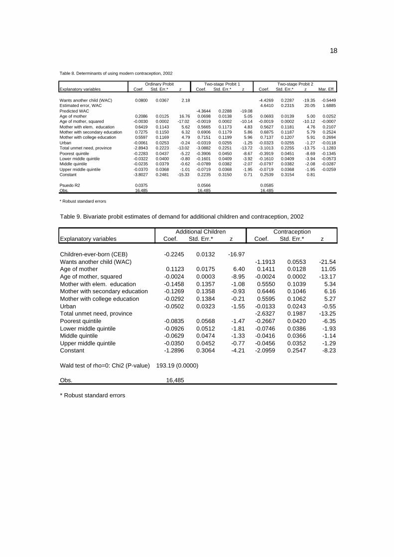
3.4.3 Use of Modern Contraception The estimation results on the use of modern contraception are given in Table 8. The demand for additional children has mixed impact on the demand for modern contraception. The coefficient is positive and significant in the ordinary probit equation but became negative and significant in the two-stage probit equations. Even more important is the significant coefficient for the estimated error term in the first stage which confirms the endogeneity of the demand for additional children variable in the contraceptive use equation and indicating the inappropriateness of the ordinary probit results. Again following the suggestion in Rivers and Vuong (1988), we will use the two-stage probit estimate in subsequent discussions. The result of the two-stage probit implies that the demand for additional children depresses the demand for modern method which agrees with expectations. The effects of the age of the mother show a rise in the demand for contraception with age at a declining rate. The impact of the education variable clearly indicates a higher demand for those with higher education with marginal effects rising from 21% with elementary education to 27% for those with college education over those with no education. Again living in urban areas has no significant impact on modern contraception adoption. The variable used to indicate the availability of family planning services, the average proportion of women with unmet need averaged at the provincial level, has the expected negative sign and is highly statistically significant. Lowering the proportion of women with unmet need by 1% increases the proportion using modern contraception by a little more than 1% as well. Finally, the use of modern contraception among women from poorer households is significantly lower relative to the richest quintile in the two-stage probit estimates. The marginal effects in the last column of the table shows that modern contraceptive prevalence of women from the poorest quintile is 13% lower than those for women in the richest quintile on the average. For women in the lower middle quintile this is lower by 6%, the middle lower by 2.9% and the upper middle by 2.6%. This result highlights the main source of the difference in unmet need for family planning – women from poorer households demand less modern methods compared to women from the richer households. 3.4.4 Bivariate Probit Results Finally, to further confirm the estimated interrelationships of the relevant variables in these equations, bivariate probit estimates were obtained to directly test the correlation between the demand for children equation and the contraception equation. The bivariate probit estimation results are given in Table 9. The computed chi-square value for the test of the correlation of the errors between the two equations is 193.19 which is highly significant confirming the earlier results from the two-stage probit. It also confirms coefficient estimates of the two-stage probit as well as provide meaningful other results. For instance, the number of children ever born is a strong significant negative determinant of the demand for additional children. The age of the mother has the usual rising at a declining rate effect. The impact of education is not significant in the demand

10

for additional children equation but positive and significant in the contraceptive demand equation. Residing in urban areas has no effect on both the demand for additional children and the contraceptive equations. The impact of socioeconomic status on the demand for additional children and demand for modern contraception has similar direction of effects as those obtained from the two-stage probit results but the significance of the coefficient is much lower. 4. Summary and Implications The cross-tabulation analyses show that, indeed there are significant differences in fertility and family planning practices across socioeconomic classes. The average children-ever-born among the poorest quintile is more than 2 children higher than the families in the richest quintile. Contraceptive prevalence is also lower among the poor. These results perhaps corroborate to yield higher unmet need for family planning among the poor compared to the women in richer households. This is not surprising as these facts are also observed in other countries as well. However, cross tabulation analysis is limited by its inability to control for other individual, household and community factors that are known to play in these relationships. A recursive discrete choice model was therefore estimated to shed light on the role of socioeconomic class measured by a wealth index on these relationships after controlling for individual, household and community characteristics. The estimation results show that children ever born are indeed higher among poorer households even after controlling for the other characteristics. The children ever born have mixed impact as a determinant of the demand for additional children. But what is interesting to observe from the results is that contrary to common expectation that the poor have higher demand for children, socioeconomic status is not a consistent significant determinant of the demand for additional children given children already born. In fact, the indication is that women from poorer households have lower demand for children relative to women from the richest quintile. This provides contrary evidence to the usual expectation that poorer families demand more children than the richer households given the ones they already have that is why they tend to have larger families. The other thing that is clear from the estimation results is that the demand for modern contraception is significantly lower among women from poorer households compared to women from richer households. This lends support to the common knowledge that women from poorer households have lower adoption rate for modern methods. Of course, this result can perhaps be viewed as the result of lower access to relatively free supplies from the public sector or lower ability to pay for supplies from the private sector. Considering the still high dependence on public supplies of women even from the richest households as shown in the cross-tabulation results there may be crowding out effect of women from poorer households contributing some more to their low demand for modern methods. Since there is no indication that these relationships have drastically changed over the years, this lower demand for modern contraception for whatever reason contributed to the higher actual number of children ever born among the poor. These results show that it may not be true that the larger family size among the poor is the result of higher demand for children. The estimation results show that given the children already born, the demand for additional children is even lower among women from poorer households compared to those from richer households. The results also show that it is true that, other things equal, the demand for modern methods is lower

11

among women from poorer households. Using the econometric as well as the cross tabulation results, this particular outcome can be the result of at least three factors: (a) been crowded out by a significant percentage of women from richer households that are also depending on public supplies of modern methods, (b) lower education of women in poorer households, and (c) lower capacity to pay for private supplies. These results imply that, in general, the Philippines has to deal with the fertility reduction issue once and for all. In addition, it puts in a better light the glaring problem of larger family size among poor households as well as the high unmet need for family planning among them. Since it is not the demand for more children but poorer fertility control that is the reason for their large family size, there is a need to focus attention on the demand for modern methods among the poor. Measures to address this issue could include: (a) subsidy for modern methods for the poor, (b) lowering the dependence of richer households on public supply, and (c) heightened advocacy for modern methods among the poor.

12

References Alonzo et al. (2004) “Population and Poverty: The Real Score,” UP School of Economics Discussion Paper 0415. Behrman, J. 1990. Human Resource Led Development? ILO-ARTEP. Behrman, J. and R. Schneider (1994). “An International Perspective on Schooling Investments in the Last Quarter Century in Some Fast-Growing East and Southeast Asian Countries,” Asian Development Review, Vol. 12, No. 2. Bollen, K., D. Guilkey and T. Mroz (1995) “Binary Outcomes and Endogenous Explanatory Variables: Tests and Solutions with an Application to the Demand for Contraceptive Use in Tunisia,” Demography 32(1), 111-131. Bollen, K., J. Glanville, and G. Stecklov (2001). “Economic Status Proxies in Studies of Fertility in Developing Countries: Does the Measure Matter? Measure Evaluation Project Working Paper Series, WP-01-38 May 2001. Bruce, J. (1990) “Fundamental Elements of the Quality of Care: A Simple Framework,” Studies in Family Planning, Vol 21. No. 2, 61-91. De dios and Associates (1993). Poverty, Growth and the Fiscal Crisis. Philippine Institute for Development Studies and International Development Research Center. Degraff, D. R. Bilsborrow and D. Guilkey (1997) “Community-level Determinants of Contraceptive Use in the Philippines: A Structural Analysis,” Demography 34(3), 385-398. Guilkey, D. and S. Jayne (1997) “Fertility Transition in Zimbabwe: Determinants of Contraceptive Use and Method Choice,” Population Studies, 51(2), 173-189. Filmer, D. and L. Pritchett (1998) “Estimating Wealth Effects without Expenditure Data – or Tears: An Application to Educational Enrollments in States of India” WPS1994 World Bank. Filmer, D. and L. Pritchett (2001) “Estimating Wealth Effects without Expenditure Data-or Tears: An Application to Education Enrollments in States of India,” Demography 38(1), 115-132. Gwatkin, D., S. Rustein, K. Johnson, R. Pande and A. Wagstaff (2000). “Socioeconomic Differences in Health, Nutrition and Population in the Philippines, Processed. World Bank. Kolenikov, S. and G. Angeles (2004) “The Use of Discrete Data in PCA: Theory, Simulations and Applications to Socioeconomic Indices,” Measure Evaluation Working Paper WP-04-85. Lee, L. (1981) “Simultaneous Equation Models with Discrete and Censored Dependent Variables, in C. Manski and D. McFadden, (eds.) Structural Analysis of Discrete Data with Economic Applications (MIT Press, Cambridge MA).

13

Madalla, G. (1983) Limited-Dependent and Qualitative Variables in Econometrics. Cambridge University Press. NSO (n.d.) “Socioeconomic Indicator to Identify the Poorest Households for Family Planning Survey and Maternal and Child Health Survey,” processed. Orbeta, A. (2005) “Poverty, Vulnerability and Family Size: Evidence from the Philippines,” Report submitted to the Asian Development Bank Institute. Orbeta, A., (2004a) “Population and Poverty at the Household Level: Revisiting the links using household surveys,” Presentation at the ICPD+10 National Conference, Heritage Hotel, Manila. October Orbeta, A. (2004b) “LGUs Need Strong National Leadership in Population Management,” PIDS Policy Note 2004-12. Orbeta, A. (2004c) “Major Findings from the Family Planning Surveys, 1995-2002,” Consultant report prepared for the “Local Enhancement and Development (LEAD) for Health,” Project. Orbeta, A. (2004d) “Major Findings from the National Demographic and Health Surveys: 1998, 1993,” Consultant report prepared for the “Local Enhancement and Development (LEAD) for Health,” Project. Orbeta, A. (2003) “Population and Poverty: A Review of the Links, Evidence and Implications for the Philippines,” Journal of Philippine Development, 30(2), 195-227. Orbeta, A. , I. Acejo, J. Cuenca, and F. del Prado (2003) “Family Planning and Maternal and Child Health Outcomes, Utilization and Access to Services by Asset Quintile,” PIDS Discussion Paper No. 2003-14. Reyes, C. (2002) “The Poverty Fight: Have We Made and Impact,” PIDS DP 2002-20. Rivers, D. and Q. Vuong (1988) “Limited Information Estimators and Exogeniety Tests for Simultaneous Probit Models,” J. of Econometrics, 39, 347-366. Sahn, David and David Stifel 2001 “Exploring Alternative Measures of Welfare in the Absence of Expenditure Data” Cornell Food and Nutrition Policy Program Working Paper No. 97.

14

Figure 1. Population Size of Selected Asian Countries, 1960-2004

0.0

20.0

40.0

60.0

80.0

100.0

Korea, Rep. Philippines Thailand Vietnam

Korea, Rep. 25.0 31.9 38.1 42.9 47.0 48.2

Philippines 27.1 36.6 48.0 61.0 76.6 83.7

Thailand 26.4 35.7 46.7 55.6 60.7 63.8

Vietnam 34.7 42.7 53.7 66.2 78.5 81.5

1960 1970 1980 1990 2000 2004

Figure 2. GDP Per Capita of Selected ASEAN Countries, Constant 1995 US$

0

1,000

2,000

3,000

4,000

Indonesia Philippines Thailand

Indonesia 249 298 503 777 1,015 1,060

Philippines 725 867 1,173 1,091 1,173 1,209

Thailand 465 752 1,116 1,997 2,828 3,000

1960 1970 1980 1990 2000 2002

Figure 3. Gross Domestic Savings of Selected Asian Countries (% GDP), 1960-2002

0.0

10.0

20.0

30.0

40.0

Indonesia Korea, Rep. Philippines Thailand

Indonesia 12.4 14.3 38.0 32.3 25.6 21.1

Korea, Rep. 2.0 15.3 24.1 36.5 31.3 27.5

Philippines 16.2 21.9 24.2 18.4 23.1 18.8

Thailand 14.1 21.2 22.9 33.8 31.4 31.1

1960 1970 1980 1990 2000 2002

15

Table 1. Mean Children Ever Born (CEB) for women 40-49 years by asset index quintile, 1999-2002

Poor-RichSurvey Year Poorest L. Middle Middle U. Middle Richest Total Diff.

2002 5.8 5.0 4.5 3.9 3.6 4.6 2.22001 5.8 5.0 4.7 3.9 3.3 4.5 2.52000 6.0 5.1 4.8 3.9 3.5 4.6 2.51999 5.9 5.2 4.9 3.9 3.5 4.6 2.3

Source: Orbeta (2004c), basic data from NSO, 1999-2002 Family Planing Surveys

Age Group No method Any Method Modern Traditional

Total 51.2 48.9 35.1 13.8

Poorest 58.5 41.5 28.0 13.5Lower Middle 50.8 49.2 35.9 13.3Middle 46.2 53.8 39.0 14.8Upper Middle 49.6 50.4 36.8 13.7Richest 49.9 50.1 36.5 13.6

Poorest/Richest Ratio 1.17 0.83 0.77 0.99

Source: Orbeta (2004c), basic data from NSO, 2002 Family Planing Survey

Table 2. Contraceptive Method by Asset Index Quintile, 2002

Method

Table 3. Source of Modern Method Supply by Method by Asset Index Quintile, 2002

Source Pill IUD Injection Diaphragm Condom Ligation Vasectomy Total

PhilippinesPublic 65.4 74.9 92.9 100.0 41.0 72.8 81.6 70.1Private 33.4 22.7 6.0 0.0 57.4 25.6 18.4 28.5PoorestPublic 87.8 86.1 96.8 0.0 78.5 84.3 100.0 87.9Private 11.7 12.1 2.2 0.0 20.2 15.6 0.0 11.4Lower MiddlePublic 75.3 83.8 96.6 100.0 56.0 85.6 100.0 80.8Private 22.9 12.8 2.4 0.0 44.1 13.2 0.0 17.6MiddlePublic 66.0 81.1 93.1 0.0 36.6 78.3 53.1 72.9Private 32.3 17.0 6.9 0.0 61.1 19.4 46.9 25.4Upper MiddlePublic 53.5 61.2 86.0 0.0 36.2 66.9 100.0 60.1Private 45.3 34.4 11.8 0.0 62.5 30.8 0.0 38.0RichestPublic 39.8 53.5 81.5 100.0 19.0 60.0 68.1 50.3Private 59.2 46.0 16.4 0.0 78.0 38.9 31.9 48.6

Poorest/Richest Ratio (%)Public 2.2 1.6 1.2 0.0 4.1 1.4 1.5 1.7Private 0.2 0.3 0.1 - 0.3 0.4 0.0 0.2


16

Table 4. Unmet Need for Family Planning, 2002

Asset IndexQuintile Total Spacing LimitingPhilippines 20.0 10.1 9.9

Poorest 27.0 13.5 13.4Lower Middle 21.7 10.3 11.5Middle 17.1 8.1 9.0Upper Middle 17.7 9.7 7.9Richest 16.0 8.8 7.2

Poorest/Richest Ratio 1.7 1.5 1.9


Table 5. Descriptive Statistics

Variable Obs Mean Std. Dev. Min Max

Children ever born 16625 3.472 2.325 0 17Wants another child 16625 0.124 0.330 0 1Use modern method 16625 0.344 0.475 0 1Age of mother 16625 35.529 8.024 15 49Mother with no education 16625 0.020 0.140 0 1Mother with elem. education 16625 0.286 0.452 0 1Mother with secondary education 16625 0.396 0.489 0 1Mother with college education 16625 0.297 0.457 0 1Urban 16485 0.606 0.489 0 1Proportion of bgy. with electricity 16485 0.808 0.176 0.251 1Proportion of bgy. with access to natinal highways 16485 0.809 0.127 0.384 1Mean income of child workers (5-14), domain level 16485 20.090 28.301 0 207Total unmet need for family planning, province level 16625 0.203 0.058 0.060 0.397

Source of basic data: 2002 FPS, NSO

17

Table 6. OLS Estimates of determinants of children ever born to married women, 2002

Explanatory variables Coef. Std. Err.* t

Age of mother 0.370 0.016 23.26Age of mother, squared -0.003 0.000 -14.12Mother with elem. education 0.325 0.172 1.89Mother with sec. education -0.212 0.172 -1.23Mother with college education -0.852 0.173 -4.91Urban -0.082 0.038 -2.17Poorest quintile 1.085 0.067 16.29Lower middle quintile 0.614 0.057 10.69Middle quintile 0.348 0.051 6.88Upper middle quintile 0.126 0.046 2.74Proportion of bgy. with electricity 0.060 0.148 0.40Proportion of bgy. with access to natinal highways -1.216 0.193 -6.31Mean income of child workers (5-14), domain level 0.001 0.001 1.45Constant -4.372 0.325 -13.45

R-square 0.339Obs. 16,485

* Robust standard errors Table 7. Determinants of demand for additional children, 2002

Explanatory variables Coef. Std. Err.* z Coef. Std. Err.* z Coef. Std. Err.* z Mar. Eff.

Children-ever-born (CEB) -0.1686 0.0120 -14.10 0.1189 0.1247 0.95 0.0151Estimated error, CEB -0.2891 0.1240 -2.33 -0.0367Predicted CEB 0.1558 0.1199 1.30Age of mother 0.1124 0.0197 5.70 -0.0094 0.0482 -0.20 0.0060 0.0501 0.12 0.0008Age of mother, squared -0.0026 0.0003 -8.42 -0.0014 0.0005 -2.70 -0.0016 0.0005 -3.08 -0.0002Mother with elem. education -0.1500 0.1384 -1.08 -0.1723 0.1385 -1.24 -0.2276 0.1430 -1.59 -0.0271Mother with secondary education -0.1255 0.1388 -0.90 0.0104 0.1383 0.08 -0.0452 0.1426 -0.32 -0.0057Mother with college education 0.0103 0.1415 0.07 0.3254 0.1743 1.87 0.2725 0.1796 1.52 0.0381Urban -0.0370 0.0346 -1.07 -0.0041 0.0386 -0.11 0.0043 0.0394 0.11 0.0006Poorest quintile -0.0660 0.0603 -1.09 -0.3830 0.1506 -2.54 -0.3955 0.1561 -2.53 -0.0426Lower middle quintile -0.0974 0.0543 -1.79 -0.2755 0.0937 -2.94 -0.2830 0.0964 -2.94 -0.0317Middle quintile -0.0314 0.0502 -0.63 -0.1304 0.0653 -2.00 -0.1333 0.0663 -2.01 -0.0160Upper middle quintile -0.0330 0.0482 -0.68 -0.0666 0.0504 -1.32 -0.0688 0.0509 -1.35 -0.0085Constant -1.3008 0.3322 -3.92 0.3152 0.7039 0.45 0.2012 0.7301 0.28

Psuedo R2 0.1869 0.1642 0.1874Obs. 16,485 16,485 16,485

* Robust standard errors

Ordinary Probit Two-stage Probit 1 Two-stage Probit 2

18

Table 8. Determinants of using modern contraception, 2002

Explanatory variables Coef. Std. Err.* z Coef. Std. Err.* z Coef. Std. Err.* z Mar. Eff.

Wants another child (WAC) 0.0800 0.0367 2.18 -4.4269 0.2287 -19.35 -0.5449Estimated error, WAC 4.6410 0.2315 20.05 1.6885Predicted WAC -4.3644 0.2288 -19.08Age of mother 0.2086 0.0125 16.76 0.0698 0.0138 5.05 0.0693 0.0139 5.00 0.0252Age of mother, squared -0.0030 0.0002 -17.02 -0.0019 0.0002 -10.14 -0.0019 0.0002 -10.12 -0.0007Mother with elem. education 0.6419 0.1143 5.62 0.5665 0.1173 4.83 0.5627 0.1181 4.76 0.2107Mother with secondary education 0.7275 0.1150 6.32 0.6906 0.1179 5.86 0.6875 0.1187 5.79 0.2524Mother with college education 0.5597 0.1169 4.79 0.7151 0.1199 5.96 0.7137 0.1207 5.91 0.2694Urban -0.0061 0.0253 -0.24 -0.0319 0.0255 -1.25 -0.0323 0.0255 -1.27 -0.0118Total unmet need, province -2.8943 0.2223 -13.02 -3.0882 0.2251 -13.72 -3.1013 0.2255 -13.75 -1.1283Poorest quintile -0.2283 0.0437 -5.22 -0.3906 0.0450 -8.67 -0.3919 0.0451 -8.69 -0.1345Lower middle quintile -0.0322 0.0400 -0.80 -0.1601 0.0409 -3.92 -0.1610 0.0409 -3.94 -0.0573Middle quintile -0.0235 0.0379 -0.62 -0.0789 0.0382 -2.07 -0.0797 0.0382 -2.08 -0.0287Upper middle quintile -0.0370 0.0368 -1.01 -0.0719 0.0368 -1.95 -0.0719 0.0368 -1.95 -0.0259Constant -3.8027 0.2481 -15.33 0.2235 0.3150 0.71 0.2539 0.3154 0.81

Psuedo R2 0.0375 0.0566 0.0585Obs. 16,485 16,485 16,485


Ordinary Probit Two-stage Probit 1 Two-stage Probit 2

Table 9. Bivariate probit estimates of demand for additional children and contraception, 2002

Explanatory variables Coef. Std. Err.* z Coef. Std. Err.* z

Children-ever-born (CEB) -0.2245 0.0132 -16.97Wants another child (WAC) -1.1913 0.0553 -21.54Age of mother 0.1123 0.0175 6.40 0.1411 0.0128 11.05Age of mother, squared -0.0024 0.0003 -8.95 -0.0024 0.0002 -13.17Mother with elem. education -0.1458 0.1357 -1.08 0.5550 0.1039 5.34Mother with secondary education -0.1269 0.1358 -0.93 0.6446 0.1046 6.16Mother with college education -0.0292 0.1384 -0.21 0.5595 0.1062 5.27Urban -0.0502 0.0323 -1.55 -0.0133 0.0243 -0.55Total unmet need, province -2.6327 0.1987 -13.25Poorest quintile -0.0835 0.0568 -1.47 -0.2667 0.0420 -6.35Lower middle quintile -0.0926 0.0512 -1.81 -0.0746 0.0386 -1.93Middle quintile -0.0629 0.0474 -1.33 -0.0416 0.0366 -1.14Upper middle quintile -0.0350 0.0452 -0.77 -0.0456 0.0352 -1.29Constant -1.2896 0.3064 -4.21 -2.0959 0.2547 -8.23

Wald test of rho=0: Chi2 (P-value) 193.19 (0.0000)

Obs. 16,485


Additional Children Contraception

19

Annex

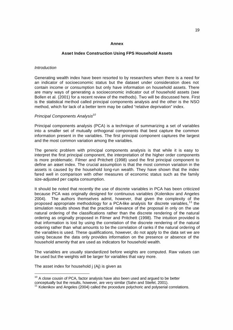
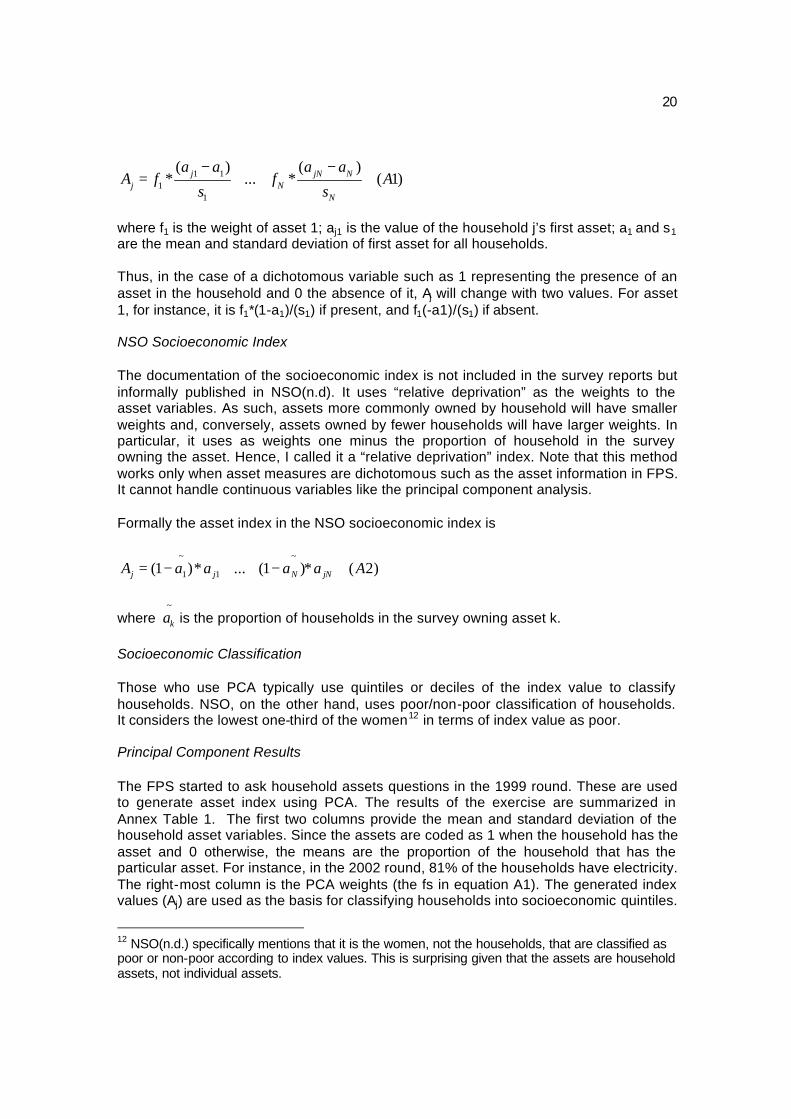
Asset Index Construction Using FPS Household Assets Introduction Generating wealth index have been resorted to by researchers when there is a need for an indicator of socioeconomic status but the dataset under consideration does not contain income or consumption but only have information on household assets. There are many ways of generating a socioeconomic indicator out of household assets (see Bollen et al. (2001) for a recent review of the methods). Two will be discussed here. First is the statistical method called principal components analysis and the other is the NSO method, which for lack of a better term may be called “relative deprivation” index. Principal Components Analysis10 Principal components analysis (PCA) is a technique of summarizing a set of variables into a smaller set of mutually orthogonal components that best capture the common information present in the variables. The first principal component captures the largest and the most common variation among the variables. The generic problem with principal components analysis is that while it is easy to interpret the first principal component, the interpretation of the higher order components is more problematic. Filmer and Pritchett (1998) used the first principal component to define an asset index. The crucial assumption is that the most common variation in the assets is caused by the household long-run wealth. They have shown that the index fared well in comparison with other measures of economic status such as the family size-adjusted per capita consumption. It should be noted that recently the use of discrete variables in PCA has been criticized because PCA was originally designed for continuous variables (Kolenikov and Angeles 2004). The authors themselves admit, however, that given the complexity of the proposed appropriate methodology for a PCA-like analysis for discrete variables, 11 the simulation results shows that the practical relevance of the proposal in only on the use natural ordering of the classifications rather than the discrete rendering of the natural ordering as originally proposed in Filmer and Pritchett (1998). The intuition provided is that information is lost by using the correlation of the discrete rendering of the natural ordering rather than what amounts to be the correlation of ranks if the natural ordering of the variables is used. These qualifications, however, do not apply to the data set we are using because the data only provides information on the presence or absence of the household amenity that are used as indicators for household wealth. The variables are usually standardized before weights are computed. Raw values can be used but the weights will be larger for variables that vary more. The asset index for household j (Aj) is given as

10 A close cousin of PCA, factor analysis have also been used and argued to be better conceptually but the results, however, are very similar (Sahn and Stiefel, 2001). 11 Kolenikov and Angeles (2004) called the procedure polychoric and polyserial correlations.

20

1 11

1

( ) ( )* ... * ( 1)j jN N

j NN

a a a aA f f A

s s

− −= + +

where f1 is the weight of asset 1; aj1 is the value of the household j’s first asset; a1 and s1 are the mean and standard deviation of first asset for all households. Thus, in the case of a dichotomous variable such as 1 representing the presence of an asset in the household and 0 the absence of it, Aj will change with two values. For asset 1, for instance, it is f1*(1-a1)/(s1) if present, and f1(-a1)/(s1) if absent. NSO Socioeconomic Index The documentation of the socioeconomic index is not included in the survey reports but informally published in NSO(n.d). It uses “relative deprivation” as the weights to the asset variables. As such, assets more commonly owned by household will have smaller weights and, conversely, assets owned by fewer households will have larger weights. In particular, it uses as weights one minus the proportion of household in the survey owning the asset. Hence, I called it a “relative deprivation” index. Note that this method works only when asset measures are dichotomous such as the asset information in FPS. It cannot handle continuous variables like the principal component analysis. Formally the asset index in the NSO socioeconomic index is

~ ~

1 1(1 )* ... (1 )* ( 2)j j N jNA a a a a A= − + + −

where ~

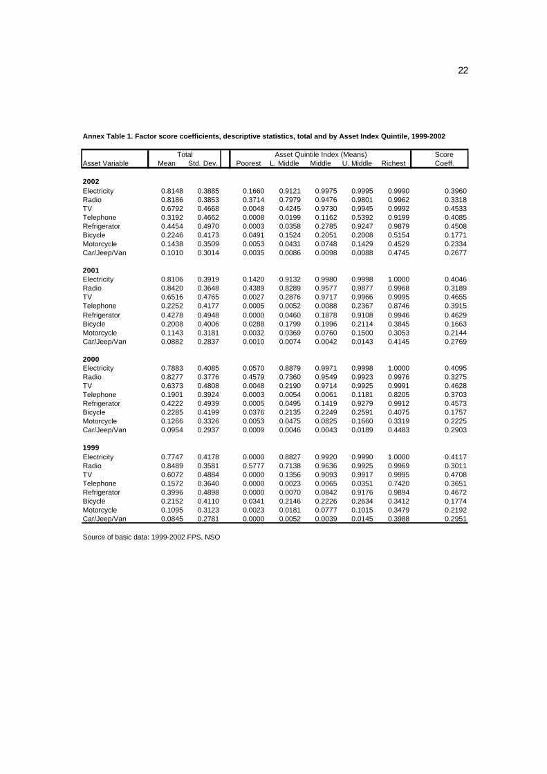
ka is the proportion of households in the survey owning asset k. Socioeconomic Classification Those who use PCA typically use quintiles or deciles of the index value to classify households. NSO, on the other hand, uses poor/non-poor classification of households. It considers the lowest one-third of the women12 in terms of index value as poor. Principal Component Results The FPS started to ask household assets questions in the 1999 round. These are used to generate asset index using PCA. The results of the exercise are summarized in Annex Table 1. The first two columns provide the mean and standard deviation of the household asset variables. Since the assets are coded as 1 when the household has the asset and 0 otherwise, the means are the proportion of the household that has the particular asset. For instance, in the 2002 round, 81% of the households have electricity. The right-most column is the PCA weights (the fs in equation A1). The generated index values (Aj) are used as the basis for classifying households into socioeconomic quintiles.

12 NSO(n.d.) specifically mentions that it is the women, not the households, that are classified as poor or non-poor according to index values. This is surprising given that the assets are household assets, not individual assets.

21

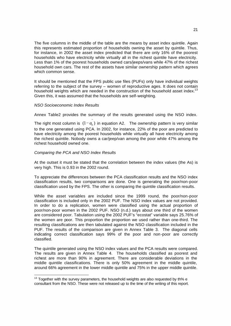
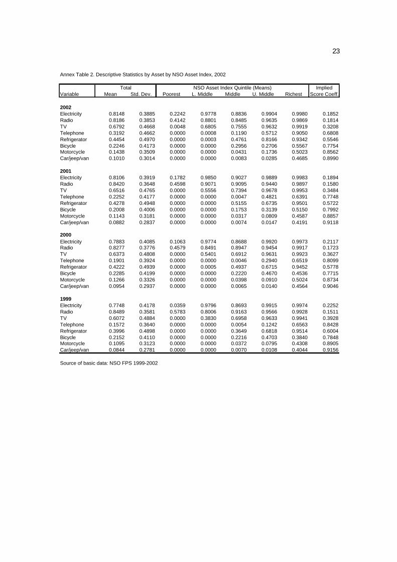
The five columns in the middle of the table are the means by asset index quintile. Again this represents estimated proportion of households owning the asset by quintile. Thus, for instance, in 2002 the asset index predicted that there are only 16% of the poorest households who have electricity while virtually all in the richest quintile have electricity. Less than 1% of the poorest households owned cars/jeeps/vans while 47% of the richest household own cars. The rest of the assets have similar ownership pattern which agrees which common sense. It should be mentioned that the FPS public use files (PUFs) only have individual weights referring to the subject of the survey – women of reproductive ages. It does not contain household weights which are needed in the construction of the household asset index.13 Given this, it was assumed that the households are self-weighting. NSO Socioeconomic Index Results Annex Table2 provides the summary of the results generated using the NSO index.

The right most column is ~

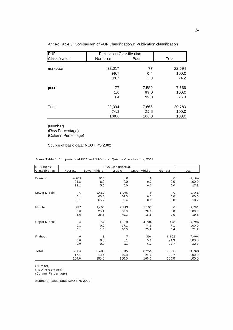
(1 )ka− in equation A2. The ownership pattern is very similar to the one generated using PCA. In 2002, for instance, 22% of the poor are predicted to have electricity among the poorest households while virtually all have electricity among the richest quintile. Nobody owns a car/jeep/van among the poor while 47% among the richest household owned one. Comparing the PCA and NSO Index Results At the outset it must be stated that the correlation between the index values (the As) is very high. This is 0.93 in the 2002 round. To appreciate the differences between the PCA classification results and the NSO index classification results, two comparisons are done. One is generating the poor/non-poor classification used by the FPS. The other is comparing the quintile classification results. While the asset variables are included since the 1999 round, the poor/non-poor classification is included only in the 2002 PUF. The NSO index values are not provided. In order to do a replication, women were classified using the actual proportion of poor/non-poor women in the 2002 PUF. NSO (n.d.) says about one third of the women are considered poor. Tabulation using the 2002 PUF’s “ecostat” variable says 25.76% of the women are poor. This proportion the proportion we used rather than one-third. The resulting classifications are then tabulated against the NSO classification included in the PUF. The results of the comparison are given in Annex Table 3. The diagonal cells indicating correct classification says 99% of the poor and non-poor are correctly classified. The quintile generated using the NSO index values and the PCA results were compared. The results are given in Annex Table 4. The households classified as poorest and richest are more than 90% in agreement. There are considerable deviations in the middle quintile classifications. There is only 50% agreement in the middle quintile, around 66% agreement in the lower middle quintile and 75% in the upper middle quintile.

13 Together with the survey parameters, the household weights are also requested by th% e consultant from the NSO. These were not released up to the time of the writing of this report.

22

Annex Table 1. Factor score coefficients, descriptive statistics, total and by Asset Index Quintile, 1999-2002

ScoreAsset Variable Mean Std. Dev. Poorest L. Middle Middle U. Middle Richest Coeff.

2002Electricity 0.8148 0.3885 0.1660 0.9121 0.9975 0.9995 0.9990 0.3960Radio 0.8186 0.3853 0.3714 0.7979 0.9476 0.9801 0.9962 0.3318TV 0.6792 0.4668 0.0048 0.4245 0.9730 0.9945 0.9992 0.4533Telephone 0.3192 0.4662 0.0008 0.0199 0.1162 0.5392 0.9199 0.4085Refrigerator 0.4454 0.4970 0.0003 0.0358 0.2785 0.9247 0.9879 0.4508Bicycle 0.2246 0.4173 0.0491 0.1524 0.2051 0.2008 0.5154 0.1771Motorcycle 0.1438 0.3509 0.0053 0.0431 0.0748 0.1429 0.4529 0.2334Car/Jeep/Van 0.1010 0.3014 0.0035 0.0086 0.0098 0.0088 0.4745 0.2677




Source of basic data: 1999-2002 FPS, NSO

Total Asset Quintile Index (Means)

23

Annex Table 2. Descriptive Statistics by Asset by NSO Asset Index, 2002

ImpliedVariable Mean Std. Dev. Poorest L. Middle Middle U. Middle Richest Score Coeff.

2002Electricity 0.8148 0.3885 0.2242 0.9778 0.8836 0.9904 0.9980 0.1852Radio 0.8186 0.3853 0.4142 0.8801 0.8485 0.9635 0.9869 0.1814TV 0.6792 0.4668 0.0048 0.6805 0.7555 0.9632 0.9919 0.3208Telephone 0.3192 0.4662 0.0000 0.0008 0.1190 0.5712 0.9050 0.6808Refrigerator 0.4454 0.4970 0.0000 0.0003 0.4761 0.8166 0.9342 0.5546Bicycle 0.2246 0.4173 0.0000 0.0000 0.2956 0.2706 0.5567 0.7754Motorcycle 0.1438 0.3509 0.0000 0.0000 0.0431 0.1736 0.5023 0.8562Car/jeep/van 0.1010 0.3014 0.0000 0.0000 0.0083 0.0285 0.4685 0.8990




Source of basic data: NSO FPS 1999-2002

Total NSO Asset Index Quintile (Means)

24

Annex Table 3. Comparison of PUF Classification & Publication classification

PUF Classification Non-poor Poor Total

non-poor 22,017 77 22,09499.7 0.4 100.099.7 1.0 74.2

poor 77 7,589 7,6661.0 99.0 100.00.4 99.0 25.8

Total 22,094 7,666 29,76074.2 25.8 100.0

100.0 100.0 100.0

(Number)(Row Percentage)(Column Percentage)

Source of basic data: NSO FPS 2002

Publication Classification

Annex Table 4. Comparison of PCA and NSO Index Quintile Classification, 2002

NSO IndexClassification Poorest Lower Middle Middle Upper Middle Richest Total

Poorest 4,789 315 0 0 0 5,10493.8 6.2 0.0 0.0 0.0 100.094.2 5.8 0.0 0.0 0.0 17.2

Lower Middle 6 3,653 1,906 0 0 5,5650.1 65.6 34.3 0.0 0.0 100.00.1 66.7 32.4 0.0 0.0 18.7

Middle 287 1,454 2,893 1,157 0 5,7915.0 25.1 50.0 20.0 0.0 100.05.6 26.5 49.2 18.5 0.0 19.5

Upper Middle 4 57 1,079 4,708 448 6,2960.1 0.9 17.1 74.8 7.1 100.00.1 1.0 18.3 75.2 6.4 21.2

Richest 0 1 7 394 6,602 7,0040.0 0.0 0.1 5.6 94.3 100.00.0 0.0 0.1 6.3 93.7 23.5

Total 5,086 5,480 5,885 6,259 7,050 29,76017.1 18.4 19.8 21.0 23.7 100.0

100.0 100.0 100.0 100.0 100.0 100.0

(Number)(Row Percentage)(Column Percentage)

Source of basic data: NSO FPS 2002

PCA Classification

poverty, fertility preferences and family planning ... · poverty, fertility preferences and family...

Documents