potential of lidar backscatter data to estimate solar aerosol radiative forcing

Potential of lidar backscatter data to estimatesolar aerosol radiative forcing

Manfred Wendisch, Detlef Müller, Ina Mattis, and Albert Ansmann

The potential to estimate solar aerosol radiative forcing (SARF) in cloudless conditions from backscatterdata measured by widespread standard lidar has been investigated. For this purpose 132 days ofsophisticated ground-based Raman lidar observations (profiles of particle extinction and backscattercoefficients at 532 nm wavelength) collected during two campaigns [the European Aerosol Research LidarNetwork (EARLINET) and the Indian Ocean Experiment (INDOEX)] were analyzed. Particle extinctionprofiles were used as input for radiative transfer simulations with which to calculate the SARF, whichthen was plotted as a function of the column (i.e., height-integrated) particle backscatter coefficient ��c�.A close correlation between the SARF and �c was found. SARF–�c parameterizations in the form ofpolynomial fits were derived that exhibit an estimated uncertainty of ��10–30�%. These parameteriza-tions can be utilized to analyze data of upcoming lidar satellite missions and for other purposes. TheEARLINET-based parameterizations can be applied to lidar measurements at mostly continental, highlyindustrialized sites with limited maritime influence (Europe, North America), whereas the INDOEXparameterizations rather can be employed in polluted maritime locations, e.g., coastal regions of southand east Asia. © 2006 Optical Society of America

OCIS codes: 010.1110, 280.1100, 280.1310, 280.3640, 290.1090.

1. Introduction

Atmospheric aerosol particles modify the Earth’s ra-diative energy budget and as a consequence affect theglobal climate, mainly as a result of scattering andabsorption of solar radiation.1 To quantify these aero-sol radiative effects, the regional distribution andsubsequent radiative influence of aerosol particleswere studied in local field campaigns; see, e.g., theoverview given by Ansmann et al.2 However, to char-acterize the emissions, to follow the transport of aero-sol particles, and to evaluate the atmospherictransformation and the respective changes in the ra-diative effects of aerosol particles on larger spatialand temporal scales require quasi-continuous andglobal observations with passive and active satellitesensors.

Unfortunately many of the passive satellite tech-niques for retrieval of aerosol-particle propertiesleave the continents blank, mostly because the influ-

ence of the bright land surfaces dominates the mea-sured radiation signal of the satellite sensors, makingit virtually impossible to retrieve aerosol-particleproperties over land. Multiangle imaging provides anew approach to separating surface from atmo-spheric signals, even over bright surfaces.3 However,such new passive observation approaches still awaitthorough validation. Also, passive satellite tech-niques, which measure the solar radiation itself, suf-fer from uncertainties that may lead to partlyconflicting results.4

Active aerosol remote-sensing techniques such aslidar, however, have been tested extensively on theground and have proved their ability to characterizeoptical and microphysical aerosol-particle prop-erties.5–7 Therefore active aerosol sensors have begunto be placed on spaceborne platforms. Thus the LidarIn-Space Technology Experiment (LITE) project8 wasconducted by NASA in 1994. Recently the CloudAerosol Lidar and Infrared Pathfinder Satellite Ob-servations9 (CALIPSO) and the Earth Clouds, Aero-sols, and Radiation Explorer10 (EarthCARE) projectswere designed. In these two collaborative effortsNASA, the Centre National de la Recherche Scienti-fique in France, the European Space Agency, and theJapan Aerospace Exploration Agency (the former Na-tional Space Development Agency of Japan) areabout, or are planning, to launch satelliteborne lidar

The authors are with the Leibniz-Institut für Troposphärenfor-schung, Permoserstrasse 15, D-04318 Leipzig, Germany. M. Wen-disch’s e-mail address is [email protected].

Received 13 June 2005; revised 8 September 2005; accepted 21September 2005.

0003-6935/06/040770-14$15.00/0© 2006 Optical Society of America

770 APPLIED OPTICS � Vol. 45, No. 4 � 1 February 2006

instruments for multiyear mapping of global aerosoldistributions.

The CALIPSO satellite will carry the first ad-vanced satelliteborne lidar system [Cloud-AerosolLidar with Orthogonal Polarization (CALIOP)] spe-cifically designed for aerosol and cloud studies. TheCALIPSO is planned to be launched in 2006 and willorbit Earth during a three-year mission. TheCALIOP will deliver profiles of the aerosol-particlebackscatter coefficient (BSC) at 532 nm wavelength.From these data the column (i.e., height-integrated)BSC of the particles ��c� at 532 nm wavelength willbe available on an operational basis. The plannedEarthCARE satellite will carry the Atmospheric Li-dar (ATLID). The measurements of �c from theCALIOP and the ATLID are expected to be of highaccuracy.

In this paper we deal with the question of whethersuch �c measurements with standard backscatter li-dar (i.e., non-Raman lidar) can be utilized to estimate(with reasonable accuracy) the radiative effects ofaerosol particles on the basis of simple parameteriza-tions, mostly without any further additional informa-tion besides �c. Such �c data not only will be availablefrom future satellite missions but were and are col-lected within numerous ground-based and airbornefield experiments. Therefore such a simple one-parameter approach could be used on many occasionsand for appropriate locations world wide, although itwill not be able to retrieve details of aerosol particles,such as their distribution with altitude and the ab-sorption effect of aerosol particles.

The radiative effect of atmospheric aerosol parti-cles can be quantified by the so-called solar aerosolradiative forcing (SARF). SARF is derived from thedifference of specific solar radiative quantities (e.g.,albedo or upwelling–downwelling irradiances at thetop or bottom of the atmosphere) with aerosol parti-cles not taken into account minus the respectivequantities including the aerosol particles. Negativevalues of SARF generally indicate solar radiativecooling; positive values, solar radiative heating of theatmosphere owing to the presence of aerosol parti-cles. Because the atmosphere is usually loaded withaerosol particles, an aerosol-free atmosphere can onlybe simulated. Thus in practice SARF cannot be ob-tained directly from measurements alone; at best it isderived from a combination of measurements andsimulations. Details of the definition of SARF aregiven in Section 3 below.

To derive the parameterizations, sophisticated li-dar observations and radiative transfer modeling arecombined. The experimental data are based onground-based observations from two intensive, long-term campaigns with Raman lidar.6,11 In contrast tostandard backscatter lidar, Raman lidar offers aunique opportunity to measure profiles of particlebackscatter and extinction coefficients simulta-neously. Therefore, on the one hand, particle extinc-tion profiles from the Raman lidar can be useddirectly for radiative transfer calculations to simulatethe SARF, and on the other hand, the corresponding

particle backscatter coefficients may serve as an in-dicator of the effects of the particles on solar radia-tion. That approach is followed in this paper. Theresultant SARF, as simulated by use of particle ex-tinction profiles from the Raman lidar, is plotted as afunction of the simultaneously measured �c; then therespective correlations are investigated. In this waythe ground-based Raman lidar data facilitate a sys-tematic study of the relationship between SARF and�c.

The Raman lidar data used in this paper stem fromtwo ground-based experiments. Anthropogenic hazeover central Europe was studied in the framework ofthe European Aerosol Research Lidar Network (EAR-LINET).12 Indo-Asian haze over the tropical IndianOcean was studied during the Indian Ocean Experi-ment (INDOEX).13 These measurements cover a widerange of possible aerosol conditions (clean and pol-luted) over the continent (EARLINET) and the ocean(INDOEX). The two experiments are briefly intro-duced in Section 2.

The particle extinction coefficient profiles retrievedfrom the Raman lidar measurements are used asinput for a radiative transfer model with which tocalculate SARF. In particular, the albedo SARF atthe top of the atmosphere (TOA) and the irradianceSARF at both the TOA and the bottom of the atmo-sphere (BOA) are investigated here. The simulationsare carried out with and without aerosol input; fromthe difference of the results of the two sets of simu-lations the SARF is calculated. These simulations areintroduced in Section 3.

In Section 4 the calculated SARF quantities areplotted versus �c measured simultaneously with theparticle extinction profiles by Raman lidar. As westressed above, �c is the only quantity that can beretrieved directly and with high accuracy fromstandard backscatter lidar observations. Correla-tions between SARF and �c are discussed and param-eterization equations (polynomial fits) are derived,whereby the dependence of the fit coefficients on solarzenith angle is explicitly considered in the fit equa-tions. In addition, a detailed uncertainty analysis ofthe SARF–�c parameterizations is performed. Bycontrasting the observations of well-defined aerosolconditions found over central Europe (EARLINET)with those measured over the Indian Ocean (IN-DOEX), we evaluate the applicability and the limitsof the polynomial fits. Finally, a summary of the pa-per is given in Section 5.

2. Observations

The EARLINET data set used in this study was de-scribed in detail by Mattis et al.11 A dual-wavelengthRaman lidar operating at 355 and 532 nm wave-lengths has routinely measured particle BSC profilesat Leipzig, Germany (51.3° N, 12.4° E), since 1997.Measuring particle extinction profiles at two wave-lengths yielded the Ångström exponent15 describingthe spectral slope of the particle extinction coefficientfor this wavelength range. Altogether, 78 lidar pro-

1 February 2006 � Vol. 45, No. 4 � APPLIED OPTICS 771

files from EARLINET, which were observed on 78days in 2000–2003, were used in the present study.

The INDOEX lidar observations have been dis-cussed by Franke et al.6 Here a six-wavelength lidarwas employed to measure the profiles of the particleBSC at 355, 400, 532, 710, 800, and 1064 nm wave-lengths and particle extinction coefficients at 355 and532 nm. In this way a characterization of the spectralslope of particle extinction from 355 to 1064 nm wasavailable from the combined particle backscatter andextinction data. The INDOEX lidar observationswere made at the Maldives International Airport atHulule Island (4.1° N, 73.3° E) in February andMarch 1999 during the intensive field phase of theINDOEX. The main goal was the characterization ofanthropogenic aerosol particles in the outflow regionsof south and east Asia. Further data were collected inJuly and October 1999 and in March 2000. TheMaldives are approximately 700 km to the southwestof the Indian subcontinent. Because of the southwestmonsoon, the Intertropical Convergence Zone wasnorth of the Maldives in July 1999, whereas it wasover Hulule Island in October 1999. These differentsituations showed the offset between continental-polluted and clean-maritime conditions over the trop-ical Indian Ocean. In total, 54 profile measurements(conducted on 54 days) from all four INDOEX cam-paigns were used for this study.

All lidar profiles were carefully screened for cloudcontamination. Clouds were unambiguously identi-fied in time–height displays of range-corrected lidarsignals. They caused a rapid increase of the backscat-ter signal with time and range. Lidar signals werestored with 30 s resolution. All signal profiles show-ing clouds were excluded from the data sets. After thecloud screening, 30–120 min average signal profileswere obtained, from which the profiles of the particleoptical properties were calculated.

In the near field of the lidar observational range (0to �1 km height; the near field of the lidar is therange of strong vertical changes of the incompleteoverlap of the laser beam with the receiver’s field ofview), we determined the particle extinction coeffi-cient profiles from the measured particle BSC by mul-tiplying the BSC by an appropriate extinction-to-backscatter ratio (lidar ratio). In the case ofEARLINET the mean lidar ratio in the height rangefrom �1 km (i.e., above the near field of the lidar) tothe top of the planetary boundary layer was used(method B; Mattis et al.11). For the INDOEX data setthe lidar ratio for the lowest 1 km altitude range wasdetermined from combined sunphotometer and lidarobservations similar to those made by Franke et al.6

From the lidar profile measurements of particleextinction coefficient � (in units of inverse meters),particle optical thickness � (dimensionless) was cal-culated by integration over height z:

� �� (z�)dz�. (1)

The column particle BSC, �c (in units of inversesteradians), was obtained by vertical integration ofthe measured profile of the particle BSC, ��z� (inunits of inverse meters per steradian):

�c �� (z�)dz�. (2)

Finally, column lidar ratio Sc (in units of steradi-ans) was derived as

Sc � �/�c. (3)

3. Atmospheric Radiative Transfer Model

The lidar profiles of ��z� were used as input for aradiative transfer model with which to calculate thebroadband solar downward and upward irradiancesat the TOA (100 km altitude) and the BOA. For thispurpose the libRadtran (Library for Radiative Trans-fer) software package of Mayer and Kylling16 wasutilized. In the simulations the discrete ordinatesolver DISORT, version 2.0, with six streams wasapplied.17 The spectral integration over the solarspectral range �250–4500 nm� was performed by useof the correlated-k approximation as suggested byKato et al.18 For the spectral surface albedo, datacollected by Wendisch et al.19 over several land (forEARLINET) and sea (for INDOEX) surfaces wereimplemented. To prescribe the gaseous compositionof the atmosphere the U.S. Standard Atmosphere (forthe EARLINET data set) and the Tropical Atmo-sphere (for INDOEX) were used; both are defined byAnderson et al.20 The radiative transfer calculationswere performed for eight values of solar zenith angle�s �10°, 30°, 50°, 65°, 70°, 75°, 80°, 85°�.

The lidar profiles of ��z� were projected onto thevertical model grid (0.1 km resolution below 6 kmaltitude and 1 km above). The spectral � values ateach altitude of the vertical model grid were thendistributed over the wavelength grid of the radiativetransfer model by use of the spectral slope given bythe Ångström parameter (derived from the lidar).Apart from the sensitivity tests described in Subsec-tion 4.C below, we fixed aerosol particle asymmetryparameter g at a value of g � 0.60, which seems to bea typical value for a wide range of aerosol condi-tions.21 Furthermore, fixed values of the aerosol par-ticle single-scattering albedo of � � 0.95 (for theEARLINET data set) and of � � 0.90 (INDOEX) havebeen assumed in the calculations. The wavelengthdependence of � was included in the simulations byuse of the Ångström parameter, whereas those of thetwo other aerosol parameters (g and �) were not in-cluded. It is well known that g and � might vary withwavelength, depending on the aerosol-particle sizedistribution, state of the mixture, refractive index ofthe particles, and particle shape. However, becausethere is nothing such as a typical spectral pattern ofboth parameters and because no actual measure-ments were available the spectral dependence of g


and � was neglected in our calculations. Instead, sev-eral tests were performed that revealed the sensitiv-ity of SARF with regard to uncertainties in g and �.In these tests the value of g was varied from 0.55 and0.65, and � was varied from 0.9 to 1.0. The range ofvalues for � was based on inversion calculations forEuropean aerosols22,23 and the Indo-Asian hazeplumes.7 The uncertainty range of g was adoptedfrom Fiebig and Ogren.21 The results of these testsare reported in Subsection 4.C below.

Two sets of calculations were made for each of themeasured ��z� profiles. For one set of results we ne-glected the aerosol-particle optical input (subscript R)and thus considered a Rayleigh atmosphere with noaerosol particles only. A second set of results wasgenerated that included the aerosol-particle opticalinput in addition to the Rayleigh contribution (sub-script AP � R). From the difference between the twosets of results the so-called SARF of the radiationquantity (albedo, irradiance) was calculated. In par-ticular, the SARF quantities were defined as follows:

A. Albedo SARF

From the ratio of the solar downward and upwardirradiances (F↓ and F↑) at the TOA, solar albedo A atthe TOA was calculated by

A �F↑(TOA)

F↓(TOA). (4)

Albedo SARF A at the TOA (dimensionless) wasthen defined by

A � AAP�R AR. (5)

By this definition it is ensured that in the aerosol-free case (no particles are present) A will vanish. Italso provides a rough separation between the influ-ence of aerosol particles on the TOA albedo on the onehand and that of the surface reflectance and of thebackscatter that is due to air molecules on the otherhand. This separation is not perfect because of non-linear interactions between the aerosol particles andthe surface–air molecules, which do not act indepen-dently of one another. Positive values of A mean anincrease of the TOA albedo caused by the aerosolparticles.

B. Irradiance SARF

Irradiance SARF F (in units of watts per squaremeter) at the top and the bottom of the atmospherewere obtained from the differences of net irradiances�F↑ F↓� at the TOA and the BOA. From this defi-nition it follows that

F(TOA) � [F↑(TOA)]R [F↑(TOA)]AP�R, (6)

F(BOA) � [F↑(BOA)F↓(BOA)]R [F↑(BOA)

F↓(BOA)]AP�R. (7)

A negative irradiance SARF at the TOA (increaseof escaping irradiance at the TOA caused by aerosolparticles) reduces the available solar energy for theatmosphere and therefore indicates a solar radiativecooling of the atmospheric column. Negative values ofF �BOA� mean a net loss of solar radiation (i.e.,cooling) of the atmosphere and a gain of solar energy(i.e., warming) of the surface.

4. Parameterization

A. Aerosol-Particle Optical Thickness

Before looking at the SARF quantities, let us explorethe correlations of aerosol-particle optical thickness �and column-particle backscatter coefficient �c (hereat 532 nm wavelength). These SARF–�c correlationplots characterize the particle optical-thicknessrange encountered during the experiments and showthe aerosol types in the two data sets from the EAR-LINET and the INDOEX. � is the major input vari-able for the radiative transfer calculations, and thusits correlation with �c will also reveal important fea-tures with which to interpret the SARF results dis-cussed afterward. It is clearly not our intention hereto investigate a parameterization of � on the basis of�c, because such correlation is simply constrained bythe column lidar ratio [Eq. (3)].

Scatterplots of � versus �c for the EARLINET dataset are displayed in Fig. 1. The data are classified in

Fig. 1. Scatterplot of particle optical thickness � as a function ofcolumn particle backscatter coefficient �c (both at 532 nm wave-length). Solid curve, polynomial fit of the data [see Eq. (8); fitcoefficients are given in Table 1). The symbols denote differentaerosol conditions in terms of column lidar ratio Sc (squares, Sc

� 70 sr; triangles, 70 sr � Sc � 50 sr; stars, 50 sr � Sc � 30 sr;pluses, Sc 30 sr). The data stem from EARLINET.


terms of column lidar ratio Sc by use of differentsymbols. Sc is characteristic for specific aerosoltypes23,24; it typically increases with the amount ofabsorption by the particles and decreases with in-creasing average particle size. For this reason mari-time aerosol populations with usually littleabsorption but containing many large particles areoften characterized by low values of Sc. At the otherextreme, polluted continental air masses with mainlysmall particles and exerting a high degree of absorp-tion normally exhibit large values of Sc.

The data plotted in Fig. 1 show a roughly linearincrease of � with �c and quite good correlation be-tween the two quantities. There are only a few datapoints with Sc 30 sr (pluses); this indicates thatmaritime aerosol types (low values of Sc) were rare inthe EARLINET data set. The pluses cover mostly lowvalues of �, which means that maritime particlesdominated on days with rather clear (i.e., low aerosolload) conditions. Data with large column lidar ratios(squares: Sc � 70 sr), however, indicating highly pol-luted air masses with mainly small and strongly ab-sorbing particles have quite frequently beenobserved. These cases occurred at low and high aero-sol loads, although most of them were observed for� � 0.2. Even though pure maritime cases were notfrequently observed in this data set, a wide range ofdifferent meteorological situations with differentaerosol types was covered.

Altogether, the entire EARLINET data set pre-sented in Fig. 1 can reasonably be approximated by alinear fit. However, a second-order polynomial fit ofthe form

�(�c) � �i�0

2

ai, ��ci, (8)

instead of a linear fit, has been chosen to fit the datapoints in Fig. 1 to help us to comprehend possibledeviations from linearity (as observed for the IN-DOEX data; see below). The solid curve in Fig. 1presents the resultant fit curve; the respective fitcoefficients ai, � �i � 0, 1, 2� are given in Table 1. Fur-thermore, the standard error of the fit, �, was calcu-lated as a measure of the expected fit uncertainty. � isalso given in Table 1. In this case (EARLINET data)the standard fit error for the optical thickness fit, ��,was 0.073.

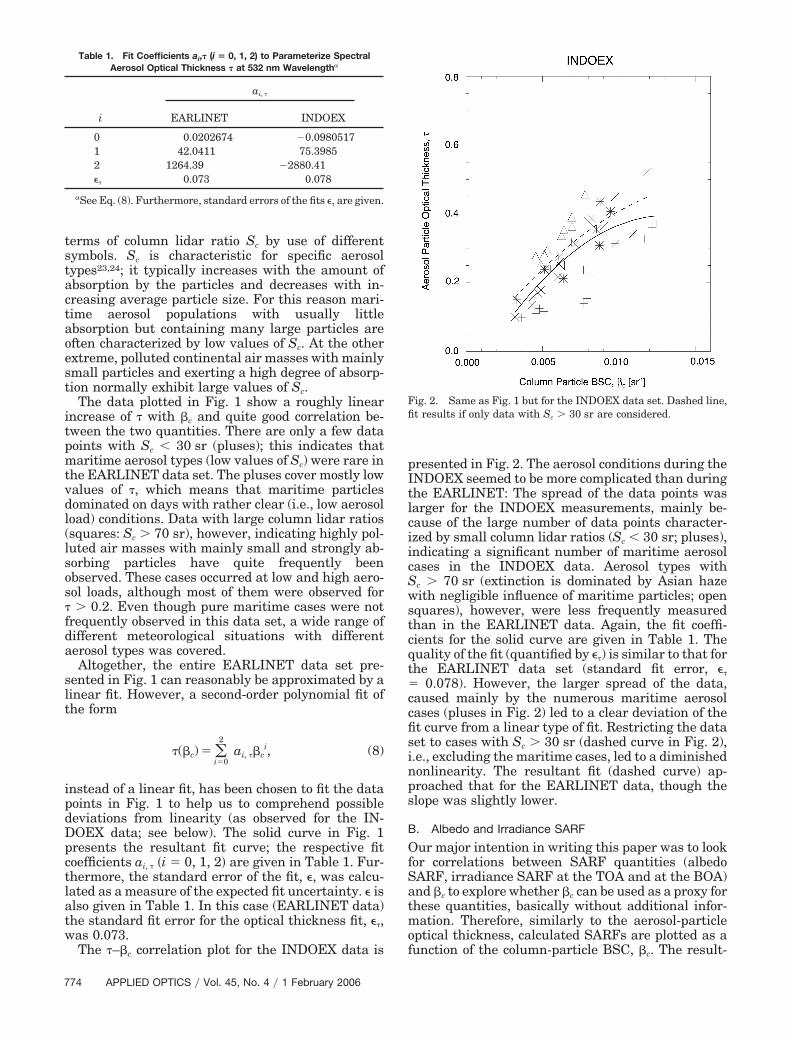
The �–�c correlation plot for the INDOEX data is

presented in Fig. 2. The aerosol conditions during theINDOEX seemed to be more complicated than duringthe EARLINET: The spread of the data points waslarger for the INDOEX measurements, mainly be-cause of the large number of data points character-ized by small column lidar ratios (Sc 30 sr; pluses),indicating a significant number of maritime aerosolcases in the INDOEX data. Aerosol types withSc � 70 sr (extinction is dominated by Asian hazewith negligible influence of maritime particles; opensquares), however, were less frequently measuredthan in the EARLINET data. Again, the fit coeffi-cients for the solid curve are given in Table 1. Thequality of the fit (quantified by ��) is similar to that forthe EARLINET data set (standard fit error, ��

� 0.078). However, the larger spread of the data,caused mainly by the numerous maritime aerosolcases (pluses in Fig. 2) led to a clear deviation of thefit curve from a linear type of fit. Restricting the dataset to cases with Sc � 30 sr (dashed curve in Fig. 2),i.e., excluding the maritime cases, led to a diminishednonlinearity. The resultant fit (dashed curve) ap-proached that for the EARLINET data, though theslope was slightly lower.

B. Albedo and Irradiance SARF

Our major intention in writing this paper was to lookfor correlations between SARF quantities (albedoSARF, irradiance SARF at the TOA and at the BOA)and �c to explore whether �c can be used as a proxy forthese quantities, basically without additional infor-mation. Therefore, similarly to the aerosol-particleoptical thickness, calculated SARFs are plotted as afunction of the column-particle BSC, �c. The result-

Table 1. Fit Coefficients ai,� (i � 0, 1, 2) to Parameterize SpectralAerosol Optical Thickness � at 532 nm Wavelengtha

i

ai, �

EARLINET INDOEX

0 0.0202674 �0.09805171 42.0411 75.39852 1264.39 �2880.41�� 0.073 0.078

aSee Eq. (8). Furthermore, standard errors of the fits �� are given.

Fig. 2. Same as Fig. 1 but for the INDOEX data set. Dashed line,fit results if only data with Sc � 30 sr are considered.


ant scatterplots are parameterized by use of polyno-mial fit equations, whereby in this case the fitcoefficients additionally depend on solar zenith angle�s. For � � A, F�TOA�, or F�BOA�, the parame-terization equations are given by

�(�c, �s) � �i�0

2

ai, �(�s)�ci. (9)

If the correlation is strictly linear, the zeroth-orderfit coefficients a0, � vanish (if there are no aerosolparticles, the SARF approaches zero), and so do thesecond-order fit coefficients a2, �. In this case a1, � rep-resents the sensitivity (slope of the fit) of the SARFquantities � with regard to changes in �c. If there aredeviations from linearity, a2, � will no longer be zeroand consequently a2, � constitutes a relative measureof deviations from linearity of the correlation fit.

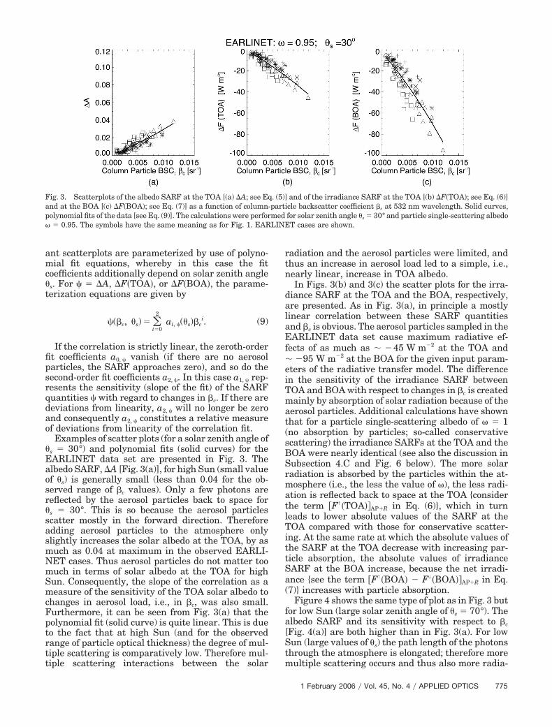
Examples of scatter plots (for a solar zenith angle of�s � 30°) and polynomial fits (solid curves) for theEARLINET data set are presented in Fig. 3. Thealbedo SARF, A [Fig. 3(a)], for high Sun (small valueof �s) is generally small (less than 0.04 for the ob-served range of �c values). Only a few photons arereflected by the aerosol particles back to space for�s � 30°. This is so because the aerosol particlesscatter mostly in the forward direction. Thereforeadding aerosol particles to the atmosphere onlyslightly increases the solar albedo at the TOA, by asmuch as 0.04 at maximum in the observed EARLI-NET cases. Thus aerosol particles do not matter toomuch in terms of solar albedo at the TOA for highSun. Consequently, the slope of the correlation as ameasure of the sensitivity of the TOA solar albedo tochanges in aerosol load, i.e., in �c, was also small.Furthermore, it can be seen from Fig. 3(a) that thepolynomial fit (solid curve) is quite linear. This is dueto the fact that at high Sun (and for the observedrange of particle optical thickness) the degree of mul-tiple scattering is comparatively low. Therefore mul-tiple scattering interactions between the solar

radiation and the aerosol particles were limited, andthus an increase in aerosol load led to a simple, i.e.,nearly linear, increase in TOA albedo.

In Figs. 3(b) and 3(c) the scatter plots for the irra-diance SARF at the TOA and the BOA, respectively,are presented. As in Fig. 3(a), in principle a mostlylinear correlation between these SARF quantitiesand �c is obvious. The aerosol particles sampled in theEARLINET data set cause maximum radiative ef-fects of as much as � 45 W m2 at the TOA and� 95 W m2 at the BOA for the given input param-eters of the radiative transfer model. The differencein the sensitivity of the irradiance SARF betweenTOA and BOA with respect to changes in �c is createdmainly by absorption of solar radiation because of theaerosol particles. Additional calculations have shownthat for a particle single-scattering albedo of � � 1(no absorption by particles; so-called conservativescattering) the irradiance SARFs at the TOA and theBOA were nearly identical (see also the discussion inSubsection 4.C and Fig. 6 below). The more solarradiation is absorbed by the particles within the at-mosphere (i.e., the less the value of �), the less radi-ation is reflected back to space at the TOA {considerthe term �F↑�TOA��AP�R in Eq. (6)}, which in turnleads to lower absolute values of the SARF at theTOA compared with those for conservative scatter-ing. At the same rate at which the absolute values ofthe SARF at the TOA decrease with increasing par-ticle absorption, the absolute values of irradianceSARF at the BOA increase, because the net irradi-ance {see the term �F↑�BOA� F↓�BOA��AP�R in Eq.(7)} increases with particle absorption.

Figure 4 shows the same type of plot as in Fig. 3 butfor low Sun (large solar zenith angle of �s � 70°). Thealbedo SARF and its sensitivity with respect to �c

[Fig. 4(a)] are both higher than in Fig. 3(a). For lowSun (large values of �s) the path length of the photonsthrough the atmosphere is elongated; therefore moremultiple scattering occurs and thus also more radia-

Fig. 3. Scatterplots of the albedo SARF at the TOA [(a) A; see Eq. (5)] and of the irradiance SARF at the TOA [(b) F�TOA�; see Eq. (6)]and at the BOA [(c) F�BOA�; see Eq. (7)] as a function of column-particle backscatter coefficient �c at 532 nm wavelength. Solid curves,polynomial fits of the data [see Eq. (9)]. The calculations were performed for solar zenith angle �s � 30° and particle single-scattering albedo� � 0.95. The symbols have the same meaning as for Fig. 1. EARLINET cases are shown.


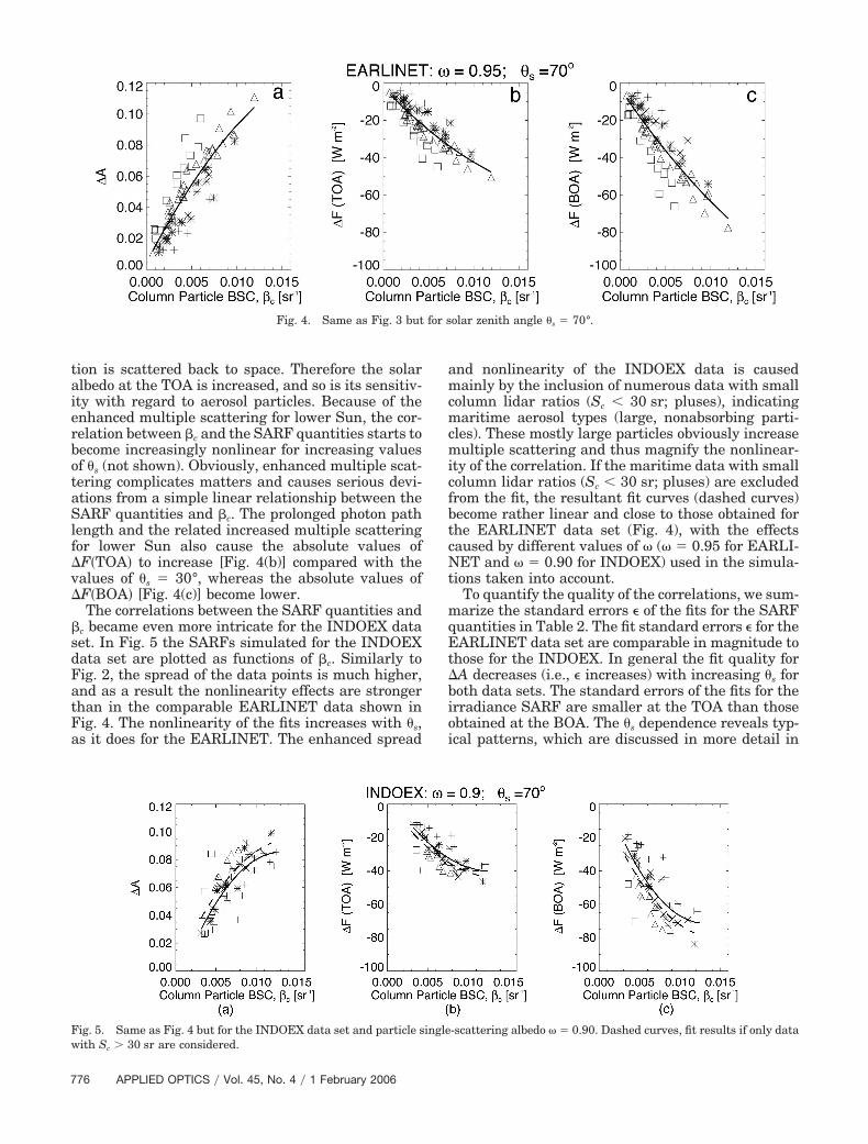
tion is scattered back to space. Therefore the solaralbedo at the TOA is increased, and so is its sensitiv-ity with regard to aerosol particles. Because of theenhanced multiple scattering for lower Sun, the cor-relation between �c and the SARF quantities starts tobecome increasingly nonlinear for increasing valuesof �s (not shown). Obviously, enhanced multiple scat-tering complicates matters and causes serious devi-ations from a simple linear relationship between theSARF quantities and �c. The prolonged photon pathlength and the related increased multiple scatteringfor lower Sun also cause the absolute values ofF�TOA� to increase [Fig. 4(b)] compared with thevalues of �s � 30°, whereas the absolute values ofF�BOA� [Fig. 4(c)] become lower.

The correlations between the SARF quantities and�c became even more intricate for the INDOEX dataset. In Fig. 5 the SARFs simulated for the INDOEXdata set are plotted as functions of �c. Similarly toFig. 2, the spread of the data points is much higher,and as a result the nonlinearity effects are strongerthan in the comparable EARLINET data shown inFig. 4. The nonlinearity of the fits increases with �s,as it does for the EARLINET. The enhanced spread

and nonlinearity of the INDOEX data is causedmainly by the inclusion of numerous data with smallcolumn lidar ratios (Sc 30 sr; pluses), indicatingmaritime aerosol types (large, nonabsorbing parti-cles). These mostly large particles obviously increasemultiple scattering and thus magnify the nonlinear-ity of the correlation. If the maritime data with smallcolumn lidar ratios (Sc 30 sr; pluses) are excludedfrom the fit, the resultant fit curves (dashed curves)become rather linear and close to those obtained forthe EARLINET data set (Fig. 4), with the effectscaused by different values of � (� � 0.95 for EARLI-NET and � � 0.90 for INDOEX) used in the simula-tions taken into account.

To quantify the quality of the correlations, we sum-marize the standard errors � of the fits for the SARFquantities in Table 2. The fit standard errors � for theEARLINET data set are comparable in magnitude tothose for the INDOEX. In general the fit quality forA decreases (i.e., � increases) with increasing �s forboth data sets. The standard errors of the fits for theirradiance SARF are smaller at the TOA than thoseobtained at the BOA. The �s dependence reveals typ-ical patterns, which are discussed in more detail in

Fig. 4. Same as Fig. 3 but for solar zenith angle �s � 70°.

Fig. 5. Same as Fig. 4 but for the INDOEX data set and particle single-scattering albedo � � 0.90. Dashed curves, fit results if only datawith Sc � 30 sr are considered.


Subsection 4.D. From Table 2 and the SARF–�c cor-relation plots, the relative deviation between theSARF quantities and the fitted data is estimated to be��10–30�% for solar zenith angles of �s 75°.

Additionally, the one-sigma standard deviation ofthe polynomial plots was calculated. The average val-ues of this quantity decrease with increasing �s. How-ever, for all cases the one-sigma average standarddeviation did not exceed �10%.

Summarizing, the scatter plots of the SARF quan-tities with the column-particle BSC reflect the�-versus-�c correlations presented in Subsection 4.Abecause � is the major input of the radiative transfermodel. The scatter in the correlation plots of theSARFs is caused mainly by the scatter in the �–�c

plots.

C. Uncertainty with Regard to Model Input

Fortunately the SARF parameters do not depend crit-ically on the vertical distribution of the optical pa-rameters that are driving the radiative transfer. Toprove this statement we performed additional radia-tive transfer simulations. First, all available particleextinction coefficient profiles (78 days from the EAR-LINET data set and 54 cases from the INDOEX cam-paign) were normalized to one common value of the(vertically integrated) particle optical thickness of0.25 (at 532 nm wavelength). This value seems quitetypical for both data sets (Figs. 1 and 2). By thisnormalization a data base consisting of strongly vari-able profiles of the particle extinction coefficient butexhibiting the same vertically integrated opticalproperty (particle optical thickness) was established.The profiles cover widely different aerosol conditions,including exponential decays, elevated aerosol layers,and well-mixed boundary layers. After the particleextinction profiles were normalized, the radiativetransfer simulations were performed to simulate theSARF quantities. In this way the calculations re-ported in this paper were repeated but the integraloptical aerosol effect (i.e., the particle optical thick-ness) was kept constant, with only the vertical dis-tribution of the optical aerosol properties (in this casethe particle extinction coefficient) varied. The resultsclearly show that the vertical stratification of the

particle extinction coefficient does not noticeably al-ter the SARF quantities.

Further sensitivity tests have proved that theSFAR–�c correlations are quite robust against differ-ent assumptions of surface albedo. The surface albe-do’s influence is mostly canceled out because for theSARF simulations differences between only the Ray-leigh (subscript R) and the Rayleigh plus aerosol(subscript AP � R) cases are considered. Also, rea-sonable variations of the Ångström parameter did notcause significant changes of the parameterizations.Changes of the Ångström parameter by as much as�20% were nearly unnoticeable in the SARF quan-tities.

So far, the remaining radiative transfer model in-put parameters (g and �) have been fixed in the sim-ulations. This assumption neglects the fact that theaerosol types change in reality and that thesechanges are reflected not only in ��z�, which has beenconsidered by use of the actual Raman lidar measure-ments in the calculations, but also in g and �, whichvary with both height z and wavelength. Thereforethe sensitivity of the SARFs to variations of �0.05 ing and � was investigated. The fitting curves, assum-ing variable values of g and � in the radiative trans-fer calculations, were simulated for different solarzenith angles �s. As an example the curves for �s

� 70° obtained for the EARLINET data set are pre-sented in Fig. 6. The solid curves with no symbols areidentical to those in Fig. 4; i.e., they are based on theinput parameters for the radiative transfer model ofg � 0.60 and � � 0.95, which represent the standardvalues in the calculations for EARLINET. For theremaining curves g was varied from 0.55 to 0.65�g � �0.05�, which corresponds roughly to a rangeof �8%. This range covered most of the values ob-served at Bondville (Illinois) and Barrow (Alaska) inrecent experiments.21 Parameter � was varied from0.9 to 1.0 (� � �0.05; i.e., �5%), which is a reason-able range for continental aerosol particles.22,23

If, for fixed �, g is increased from g � 0.60 (solidcurves with no symbols in Fig. 6) to g � 0.65 (dottedcurves), then the albedo SARF �A� decreasesslightly, and so do the absolute values of the irradi-ance SARF at the TOA and the BOA. A larger asym-

Table 2. Fit Standard Errors � for the Parameterizations of Albedo SARF at the TOA, ��A, and the Irradiance SARF at the TOA, ��F(TOA), and at theBOA, ��F(BOA)

EARLINET INDOEX

�s (°) ��A ��F(TOA) (W m�2) ��F(BOA) (W m�2) ��A ��F(TOA) (W m�2) ��F(BOA) (W m�2)

10 0.0029 3.9 9.1 0.0021 2.8 8.030 0.0038 4.5 9.5 0.0026 3.1 8.150 0.0064 5.6 10.1 0.0041 3.6 8.165 0.0106 6.1 9.7 0.0065 3.8 7.370 0.0127 5.9 8.9 0.0078 3.6 6.675 0.0152 5.4 7.6 0.0094 3.3 5.680 0.0178 4.2 5.5 0.0112 2.6 4.085 0.0190 2.2 2.5 0.0121 1.4 1.8


metry of the aerosol-particle phase function,represented by the larger g, causes more forwardscattering, which in turn reduces the solar albedo atthe TOA and the absolute values of the irradianceSARF. The opposite behavior was observed when gwas decreased from g � 0.60 (solid curves withoutsymbols) to g � 0.55 (dashed curves), again for fixed�. Altogether the effects of varying g (by �0.05) onA, F�TOA�, and F�BOA� for a solar zenith angleof �s � 70° were in the range of �9%. This influenceis smaller than the relative standard error of theparameterizations [see Table 2, ��10–30�%] and is inthe relative g-variation range itself.

The variations of � (solid curves with symbols inFig. 6) for fixed values of g exercised larger effects onthe fit curves for A, F�TOA�, and F�BOA�. Stron-ger absorption (� � 0.90, open triangles) significantlyreduced the albedo SARF [Fig. 6(a)], whereas dimin-ished absorption (� � 1.00, open squares) caused theopposite reaction, i.e., an increase of the albedoSARF. The effects of varying the values of � on theTOA and BOA irradiance SARFs turned out to bemore complex. Increased absorption [� � 0.90, opentriangles in Figs. 6(b) and 6(c)] reduced the absolutevalues of the irradiance SARF at the TOA and in-creased this quantity at the BOA by approximatelythe same amount. The reasons for this different be-havior were already discussed in Subsection 4.B. Forconservative scattering [� � 1.00, open squares inFigs. 6(b) and 6(c)] the irradiance SARF at the TOAwas nearly identical to that at the BOA, a fact thatalso was discussed, in Subsection 4.B. Altogether theeffects of variations of � of �0.05 on A, F�TOA�,and F�BOA� are �17% for �s � 70°, which is stillinside the fit’s standard errors ��10–30�%�.

The radiative transfer simulations with varying par-ticle asymmetry parameter g and single-scattering al-bedo � were performed for several values of solarzenith angle �s. Table 3 summarizes the average effect

(averaged over the �c range investigated) of theparameter variations on the SARF quantities for thetwo values �s � 70° and �s � 30° for the EARLINETdata set. Both the absolute and the relative (in pa-rentheses) values of the averaged effects are given.For high Sun (small �s) the absolute values of �A aresmaller than for low Sun; for the relative values of �A

the opposite is true. The absolute values of �A areclearly less than the fit standard errors for the albedoSARF ��A� given in Table 2 for EARLINET; thus �A

is within the spread of the respective correlationplots. This holds for most of the values in Table 3.From these numbers in Tables 2 and 3 it is concludedthat if SARF quantities A, F�TOA�, and F�BOA�are parameterized in terms of �c, an overall uncer-tainty of ��10–30�% (determined by the parameter-ization uncertainty) has to be taken into account.

D. Dependence of SARF versus �c Correlation on SolarZenith Angle

The SARF-versus-�c correlations have been calcu-lated and plotted for eight values of the solar zenith

Fig. 6. Same as Fig. 4 but without the scatterplot points; only the parameterization curves are shown. Different input combinations havebeen used for the parameterization. Solid curves are computed for aerosol-particle asymmetry parameter g � 0.60; particle single-scattering albedo � � 0.95 (the solid curves are identical to those in Fig. 4). The remaining curves are marked as follows: dotted curves,g � 0.65 and � � 0.95; dashed curves, g � 0.55 and � � 0.95; solid curves with open triangles, g � 0.60 and � � 0.90; solid curves withopen squares, g � 0.60 and � � 1.00. The data stem from EARLINET. The calculations were performed for a solar zenith angle�s � 70°.

Table 3. Average Effect � (Averaged over the �c Range Investigated) ofChanges of �g � �0.05 and �� 0.05 on the Albedo SARF, ��A, and

the Irradiance SARF at the TOA, ��F(TOA), and the BOA, ��F(BOA)a

�s

EARLINET

�A �F�TOA� �W m2� �F�BOA� �W m2�

g �

�0.05w �

�0.05g �

�0.05w �

�0.05g �

�0.05w �

�0.05

30° 0.002 0.004 2.7 4.7 3.0 8.6(19) (32) (19) (32) (10) (29)

70° 0.004 0.008 1.8 3.8 1.7 4.9(9) (17) (9) (17) (6) (15)

aIn parentheses the average relative effect is given in percent.


angle ��s � 10°, 30°, 50°, 65°, 70°, 75°, 80°, 85°� andfitted to polynomials by use of Eq. (9) for each valueof �s. Instead of providing lookup tables of the fitcoefficients for all these situations, we have plottedpolynomial fit coefficients ai, � as a function of �s inFig. 7 (EARLINET) and in Fig. 8 (INDOEX). Fromthese data the �s-dependent fit coefficients ai, ��s�were parameterized as fifth-order polynomials:

aj, �(�s) � �j�0

5

bj, ��sj. (10)

Using the resultant polynomial fit coefficientsgiven in Table 4 and Eqs. (9) and (10) allow us toestimate the SARF quantities [A, F�TOA�, andF�BOA�] as functions of column particle BSC �c,with the solar zenith angle �s as a free parameter.

Figure 7 shows the polynomial fit coefficients

ai, � �i � 0, 1, 2� as a function of �s for the EARLINETdata set. The zeroth-order coefficients [Figs. 7(a),7(d), and 7(g)] are close to zero. This is a kind ofquality check for the polynomial fit. In theory, thosezeroth-order coefficients should always vanish. Ifthere is no aerosol (i.e., if �c is identical to zero), theSARF should be zero as well. This condition is ful-filled well for the EARLINET data set for values of �s

of less than approximately 75°–80°. Anyway, the re-sults of the radiative transfer model for solar zenithangles larger than 80° should be interpreted withcaution, because a plane-parallel geometry has beenassumed in the simulations. The effects of Earth sur-face curvature, which become noticeable for very lowSun ��s � 82°�,25 have not been considered here.

The absolute values of the first-order polynomialcoefficients [Figs. 7(b), 7(e), and 7(h)] can be inter-preted as the sensitivity of the respective SARF

Fig. 7. Parameterization coefficients ai, A, ai, F�TOA�, and ai, F�BOA� �i � 0, 1, 2� for (a)–(c) the albedo SARF at the TOA and the irradianceSARF at (d)–(f) the TOA and (g)–(i) the BOA as functions of solar zenith angle �s. The data stem from the EARLINET data set. Solid curves,polynomial fits of the data [see Eq. (10); fit coefficients are given in the top of Table 4.


quantity with respect to �c if a linear correlation ismaintained (as is mostly the case for the EARLINETdata set). For the albedo SARF [Fig. 7(b)] this sensi-tivity gradually increases with �s. The lower the Sun,the more important is the effect of the aerosol parti-cles for the albedo at the TOA because for decliningSun the interactions between the photons and theparticles increase (larger photon path length, in-creased multiple scattering). For the irradianceSARF [Figs. 7(e) and 7(h)] the aerosol sensitivity in-creases with �s until a minimum is reached near �s

� 70°; from there the aerosol sensitivity decreasesagain. This is a typical pattern, which is caused bytwo competing effects. On the one hand the sensitiv-ity increases with �s because of enhanced multiplescattering and prolonged photon path length. On theother hand, for increasing values of �s, fewer andfewer photons penetrate the entire atmosphere, thusdecreasing the number of interactions between the

photons and the particles. Whereas the first effectdominates for �s 70°, the second effect turns out tobe preponderant for larger values of solar zenith an-gles.

The absolute values of the second-order polyno-mial coefficients [Figs. 7(c), 7(f), and 7(i)] can beinterpreted as a relative measure of the nonlinear-ity of the fit. Increasing absolute values of thesecond-order polynomial coefficients indicate in-creasing deviations from a linear fit. For the albedoSARF the nonlinearity of the A-versus-�c correla-tion fits increases continuously with increasing �s.The more multiple scattering occurs and the longerthe photon path lengths are, the more complicated(i.e., nonlinear) the A–�c correlation becomes, andthus the more deviations from a linear correlation fitare observed. For the irradiance SARF at the TOAand the BOA, the relative �s courses are similar tothose for the first-order polynomial coefficients,

Fig. 8. Same as Fig. 7 but for the INDOEX data set and particle single-scattering albedo � � 0.90. The fit coefficients are given in thetop of Table 4.


though opposite in sign. The interpretations of thecurves are similar.

Using the polynomial coefficients given in Table 4for the EARLINET data, one can calculate estimatesof the SARF for the EARLINET data set as a functionof �c and of �s.

In Fig. 8 polynomial coefficients ai, � �i � 0, 1, 2� areplotted for the INDOEX data. Again, the fifth-orderpolynomial fits were included in the figure as solidcurves. Compared with those in Fig. 7, the zeroth-order coefficients deviated more strongly from zero.This indicates a generally poorer fit quality, which iscaused mainly by the occurrence of cases with a dom-inant influence of maritime particles �Sc 30 sr� inthe INDOEX data set. The sensitivity of the SARFs isgenerally larger for the INDOEX data (see first-orderpolynomial coefficients), and so are the deviationsfrom linearity (second-order polynomial coefficients).The polynomial coefficients of the fits in Fig. 8 aregiven in the data sets for the INDOEX in Table 4.

5. Summary and Discussion

On the basis of a comprehensive set of sophisticatedground-based Raman lidar profile measurements of

aerosol-particle backscatter and extinction coeffi-cients from two campaigns (EARLINET andINDOEX), which cover a wide range of possible aero-sol situations, parameterizations to estimate solaraerosol radiative forcing (SARF) have been derived.For this purpose the Raman lidar profile measure-ments of particle extinction coefficients were used asinput for radiative transfer calculations. The simula-tions yielded the SARF, which was then plotted as afunction of the column (i.e., height-integrated) parti-cle backscatter coefficient ��c�. �c was measured si-multaneously with the particle extinction coefficientprofiles by Raman lidar. The resultant scatter plotswere parameterized by use of polynomial fits.

A good fit quality of the SARF was observed for theEARLINET data set, which included mostly conti-nental aerosol types (moderate absorption) but alsocontained some (though less frequent) maritime aero-sol situations. For high Sun (small values of solarzenith angle �s) the correlation was nearly linear; forlarger values of �s the fit curves became increasinglynonlinear. This was caused by prolonged photon pathlengths and the resultant enhanced multiple scatter-ing for low Sun for increased values of �c.

Table 4. Fit Coefficients bj, �A, bj,F(TOA), and bj,F(BOA) (j�0,. . . ,5) to Parameterize Fit Coefficients ai,A, ai,F(BOA), and ai,F(TOA) (i�0,1,2) for the AlbedoSARF at the TOA, A, and the Irradiance SARF at the TOA, F(TOA), and at the BOA, F(BOA))a

Parameterizations for the EARLINET data set

A b0, A b1, A b2, A b3, A b4, A b5, A

a0, A �0.0242266 0.00451036 �0.000262497 6.70485 � 106 7.83892 � 108 3.45850 � 1010

a1, A 16.1340 �2.64061 0.152705 �0.00380248 4.32416 � 105 1.79799 � 107

a2, A �503.822 101.171 �5.73935 0.140258 �0.00153767 6.01697 � 106

F�TOA� b0, F�TOA� b1, F�TOA� b2, F�TOA� b3, F�TOA� b4, F�TOA� b5, F�TOA�

a0, F�TOA� �3.92047 0.546980 �0.0319254 0.000802533 9.21467 � 106 3.90602 � 108

a1, F�TOA� �3891.40 346.964 �21.8857 0.577431 �0.00739729 3.64806 � 105

a2, F�TOA� 127338. �38110.4 2275.58 �59.1141 0.716736 �0.00323376

F�BOA� b0, F�BOA� b1, F�BOA� b2, F�BOA� b3, F�BOA� b4, F�BOA� b5, F�BOA�

a0F�BOA� �7.08587 0.868169 �0.0500522 0.00125157 1.42286 � 105 5.99614 � 108

a1, F�BOA� �6631.38 322.184 �20.6101 0.557597 �0.00738187 3.80091 � 105

a2, F�BOA� 99665.3 �48246.4 2895.67 �75.4873 0.922491 �0.00419713

Parameterizations for the INDOEX data set

A b0, A b1, A b2, A b3, A b4, A b5, A

a0, A �0.0545145 0.00917684 �0.000535120 1.36040 � 105 1.58723 � 107 6.94176 � 1010

a1, A 21.8979 �3.32518 0.192997 �0.00482700 5.53033 � 105 2.33139 � 107

a2, A �834.159 126.970 �7.36130 0.183806 �0.00210022 8.81309 � 106

F�TOA� b0, F�TOA� b1, F�TOA� b2, F�TOA� b3, F�TOA� b4, F�TOA� b5, F�TOA�

a0, F�TOA� 1.79998 0.735887 �0.0406182 0.000997268 1.05549 � 105 3.76067 � 108

a1, F�TOA� �6342.82 264.156 �17.2693 0.465143 �0.00618695 3.23002 � 105

a2, F�TOA� 253212. �12641.6 810.740 �21.7033 0.283137 �0.00143807

F�BOA� b0, F�BOA� b1, F�BOA� b2, F�BOA� b3, F�BOA� b4, F�BOA� b5, F�BOA�

a0, F�BOA� 7.87148 1.42642 �0.0808956 0.00201754 2.21702 � 105 8.40544 � 108

a1, F�BOA� �14495.8 190.286 �12.7915 0.361999 �0.00518459 3.04847 � 105

a2, F�BOA� 579992. �16127.4 1003.04 �26.8006 0.348517 �0.00180948

aSee Eq. (10). The parameterizations are valid for the eight solar zenith angles only; between the angles the curves should beinterpolated.


For the INDOEX measurements the circumstanceswere more difficult. The spread of the data of thecorrelation plots was larger than for EARLINETdata, mainly because the INDOEX data set containeda quite large number of clear maritime aerosol situ-ations (small column lidar ratio). This caused stron-ger deviations from the linearity of the polynomialfits.

Altogether an uncertainty of the SARF as obtainedfrom the polynomial fit equations of ��10–30�% wasestimated. This error assessment includes uncertain-ties that are due to the parameterization itself andadditional errors that are due to reasonable devia-tions of particle asymmetry parameter g and single-scattering albedo � from those values assumed in theradiative transfer simulations. The estimates of theSARF will get increasingly uncertain if cases withdominant maritime aerosol conditions (e.g., large,nonabsorbing sea salt particles) prevail.

The derived polynomial fits can be used to estimateSARF based on measurements of the column (i.e.,height-integrated) particle backscatter coefficient��c�. Such data are widely available from widespreadground-based and airborne standard backscatter li-dar and will increasingly more often be obtained fromfuture spaceborne missions such as CALIPSO andEarthCARE. Whereas the parameterization equa-tions derived from the EARLINET data can be ap-plied for rather continental, highly industrializedsites (Europe, North America) with limited maritimeinfluence and less absorption owing to the aerosolparticles, the INDOEX parameterizations should beemployed for polluted maritime locations, i.e., coastalregions of less developed, highly polluted areas (in-cluding some fraction of highly absorbing aerosol par-ticles) such as south and east Asia.

General attention is needed in applying the derivedfit equations, which serve as a first attempt to enableestimates of SARF to be made from simple standardbackscatter lidar measurements. It is evident that aone-parameter parameterization of such a compli-cated quantity as the SARF cannot completely coverall interactions. Therefore the approach is not fullycapable of identifying in detail special aerosol fea-tures such as forest fires and volcanic eruptions. Suchcomprehensive coverage cannot be expected from theone-parameter approach and was also not our inten-tion for this study. The polynomial fit equations arebased on radiative transfer simulations that use fixedvalues of the aerosol-particle asymmetry parameter�g � 0.6� and particle single-scattering albedo(� � 0.95 for EARLINET; � � 0.90 for INDOEX).Reasonable deviations ��0.05� from the fixed valuesof g and � were considered in the overall estimate ofthe parameterization uncertainty ��10–30�%�.However, if the values of g and � are outside therange considered in the uncertainty analysis �g� 0.55–0.65; � � 0.90–1.00�, larger deviations of theparameterized SARF will have to be taken into ac-count. Certainly future research is needed to look inmore detail at the influence of the a priori unknownvalues of particle asymmetry parameter g, and in

particular of particle single-scattering albedo � onthe derived SARF quantities.

We are grateful to Jost Heintzenberg (Institut fürTroposphärenforschung, Leipzig, Germany) and BobCharlson and Tad Anderson (University of Washing-ton, Seattle) for initiating this study and for theiruseful comments on an earlier version of this paper.

References1. R. J. Charlson and J. Heintzenberg, Aerosol Forcing of Climate

(Wiley, 1995).2. A. Ansmann, U. Wandinger, A. Wiedensohler, and U. Leiterer,

“Lindenberg Aerosol Characterization Experiment 1998(LACE 98): overview,” J. Geophys. Res. 107, doi:10.1029�2000JD000233 (2002).

3. R. A. Kahn, B. J. Gaitley, J. V. Martonchik, D. J. Diner, K. A.Crean, and B. Holben, “Multiangle Imaging Spectroradiometer(MISR) global aerosol optical depth validation based on 2 yearsof coincident Aerosol Robotic Network (AERONET) observa-tions,” J. Geophys. Res. 110, D10S04, doi:10.1029�2004JD004706 (2005).

4. B. A. Wielicki, T. Wong, N. Loeb, P. Minnis, K. Priestley, andR. Kandel, “Changes in Earth’s albedo measured by satellites,”Science 308, 825 (2005).

5. J. Redemann, R. P. Turco, K. N. Liou, P. B. Russell, R. W.Bergstrom, B. Schmid, J. M. Livingston, P. V. Hobbs, W. S.Hartley, S. Ismail, R. A. Ferrare, and E. V. Browell, “Retriev-ing the vertical structure of the effective aerosol complex indexof refraction from a combination of aerosol in situ and remotesensing measurements during TARFOX,” J. Geophys. Res.105, 0148-0227�00�1999JD901044 (2000).

6. K. Franke, A. Ansmann, D. Müller, D. Althausen, C. Venkat-araman, M. S. Reddy, F. Wagner, and R. Scheele, “Opticalproperties of the Indo-Asian haze layer over the tropical IndianOcean,” J. Geophys. Res. 108, doi:10.1029�2002JD002473(2003).

7. D. Müller, K. Franke, A. Ansmann, D. Althausen, and F. Wag-ner, “Indo-Asian pollution during INDOEX: microphysical par-ticle properties and single scattering albedo inferred frommultiwavelength lidar observations,” J. Geophys. Res. 108,doi:10.1029�2003JD003538 (2003).

8. M. P. McCormick, D. M. Winker, E. V. Browell, J. A. Coakley,C. S. Gardner, R. M. Hoff, G. S. Kent, S. H. Melfi, R. T. Men-zies, C. M. R. Platt, D. A. Randall, and J. A. Reagan, “Scientificinvestigations planned for the Lidar In-space Technology Ex-periment (LITE),” Bull. Am. Meteorol. Soc. 74, 205–214 (1993).

9. D. M. Winker, J. R. Pelon, and M. P. Cormick, “The CALIPSOmission: spaceborne lidar for observation of aerosols andclouds,” in Lidar Remote Sensing for Industry and Environ-ment Monitoring III, U. N. Singh, T. Itabe, and Z. Liu, eds.,Proc. SPIE 4893, 1–11 (2003).

10. European Space Agency, “EarthCARE–Earth clouds, aerosols,and radiation explorer,” Rep. ESA SP-1257 (1) (EuropeanSpace Research and Technology Center, 2001), http://ravel.esrin.esa.it/docs/sp_1257_1_earthcaresc.pdf (2001).

11. I. Mattis, A. Ansmann, D. Müller, U. Wandinger, and D. Al-thausen, “Multi-year aerosol observations with dual-wavelength Raman lidar in the framework of EARLINET,” J.Geophys. Res. 109, doi:10.1029�2004JD004600 (2004).

12. J. Bösenberg, V. Matthias, A. Amodeo, V. Amiridis, A. Ans-mann, J. M. Baldasano, I. Balin, D. Balis, C. Böckmann, A.Boselli, G. Carlsson, A. Chaikovsky, G. Chourdakis, A. Com-erón, F. De Tomasi, R. Eixmann, V. Freudenthaler, H. Giehl,I. Grigorov, A. Hågåd, M. Iarlori, A. Kirsche, G. Kolarov, L.Konguem, S. Kreipl, W. Kumpf, G. Larchevêque, H. Linné, R.Matthey, I. Mattis, A. Mekler, I. Mironova, V. Mitev, L. Mona,


D. Müller, S. Music, S. Nickovic, M. Pandolfi, A. Papayannis,G. Pappalardo, J. Pelon, C. Perez, R. M. Perrone, R. Persson,D. P. Resendes, V. Rizi, F. Rocadenbosch, J. A. Rodrigues, L.Sauvage, L. Schneidenbach, R. Schumacher, V. Shcherbakov,V. Simeonov, P. Sobolewski, N. Spinelli, I. Stachlewska, D.Stoyanov, T. Trickl, G. Tsaknakis, G. Vaughan, U. Wandinger,X. Wang, M. Wiegner, M. Zavrtanik, and C. Zerefos, “EARLI-NET: a European Aerosol Research Lidar Network to establishan aerosol climatology,” Report 348 (Max-Planck-Institut fürMeteorologie, 2003).

13. V. Ramanathan, P. J. Crutzen, J. Lelieveld, A. P. Mitra, D.Althausen, J. Anderson, M. O. Andreae, W. Cantrell, G. R.Cass, C. E. Chung, A. D. Clarke, J. A. Coakley, W. D. Collins,W. C. Conant, F. Dulac, J. Heintzenberg, A. J. Heymsfield, B.Holben, S. Howell, J. Hudson, A. Jayaraman, J. T. Kiehl, T. N.Krishnamurti, D. Lubin, G. McFarquhar, T. Novakov, J. A.Ogren, I. A. Podgorny, K. Prather, K. Priestley, J. M. Prospero,P. K. Quinn, K. Rajeev, P. Rasch, S. Rupert, R. Sadourny, S. K.Satheesh, G. E. Shaw, P. Sheridan, and F. P. J. Valero, “IndianOcean Experiment: an integrated analysis of the climate forc-ing and effects of the great Indo-Asian haze,” J. Geophys. Res.106, 371–398 (2001).

14. A. Ansmann, U. Wandinger, M. Riebesell, C. Weitkamp, andW. Michaelis, “Independent measurement of extinction andbackscatter profiles in cirrus clouds by using a combined Ra-man elastic-backscatter lidar,” Appl. Opt. 31, 7113–7131(1992).

15. A. Ångström, “The parameters of atmospheric turbidity,” Tel-lus 16, 64–75 (1964).

16. B. Mayer and A. Kylling, “Technical note: The libRadtran soft-ware package for radiative transfer calculations—descriptionand examples of use,” Atmos. Chem. Phys. 5, 1855–1877(2005).

17. K. Stamnes, S. C. Tsay, W. Wiscombe, and K. Jayaweera, “Anumerically stable algorithm for discrete-ordinate-method ra-

diative transfer in multiple scattering and emitting layeredmedia,” Appl. Opt. 27, 2502–2509 (1988).

18. S. Kato, T. P. Ackerman, J. H. Mather, and E. E. Clothiaux,“The k-distribution method and correlated-k approximation fora shortwave radiative transfer model,” J. Quant. Spectrosc.Radiat. Transfer 62, 109–121 (1999).

19. M. Wendisch, P. Pilewskie, E. Jäkel, S. Schmidt, J. Pommier,S. Howard, H. H. Jonsson, H. Guan, M. Schröder, and B.Mayer, “Airborne measurements of areal spectral surface al-bedo over different sea and land surfaces,” J. Geophys. Res.109, D08203, doi:10.1029�2003JD004392 (2004).

20. G. P. Anderson, S. A. Clough, F. X. Kneizys, J. H. Chetwynd,and E. P. Shettle, “AFGL atmospheric constituent profiles�0–120 km�,” Rep. AFGL-TR-86-0110 (U.S. Air Force Geophys-ics Laboratory, 1986).

21. M. Fiebig and J. A. Ogren, “Retrieval and climatology of theaerosol asymmetry parameter in the NOAA aerosol monitor-ing network,” submitted to J. Geophys. Res.

22. U. Wandinger, D. Müller, C. Böckmann, D. Althausen, V. Mat-thias, J. Bösenberg, V. Weiss, M. Fiebig, M. Wendisch, A.Stohl, and A. Ansmann, “Optical and microphysical character-ization of biomass-burning and industrial-pollution aerosolsfrom multiwavelength lidar and aircraft measurements,” J.Geophys. Res. 107, doi:10.1029�2000JD0002002 (2002).

23. D. Müller, A. Ansmann, F. Wagner, K. Franke, and D. Al-thausen, “European pollution outbreaks during ACE2: micro-physical particle properties and single-scattering albedoinferred from multiwavelength lidar data,” J. Geophys. Res.107, doi:10.1029�2001JD001110 (2002).

24. A. Ansmann, F. Wagner, D. Müller, D. Althausen, A. Herber,W. von Hoyningen-Huene, and U. Wandinger, “European pol-lution outbreaks during ACE 2: optical particle properties in-ferred from multiwavelength lidar and star�Sun photometry,”J. Geophys. Res. 107, doi:10.1029�2001JD001109 (2002).

25. G. E. Thomas and K. Stamnes, Radiative Transfer in the At-mosphere and Ocean (Cambridge U. Press, 1999).


potential of lidar backscatter data to estimate solar aerosol radiative forcing

Documents