NASA/TM-2000-206892, Vol. 11

SeaWiFS Postlaunch Technical Report Series

Stanford B. Hooker and Elaine R. Firestone, Editors

Volume 11, SeaWiFS Postlaunch Calibration andValidation Analyses, Part 3

John E. 0 'Reilly, St_phane Maritorena, Margaret C. O'Brien, David A. Siegel, Dierdre Toole,

David Menzies, Raymond C. Smith, James L. Mueller, B. Greg Mitchell, Mati Kahru,

Francisco P. Chavez, P. Strutton, Glenn E Cota, Stanford B. Hooker, Charles R. McClain,

Kendall L. Carder, Frank M_ller-Karger, Larry Harding, Andrea Magnuson, David Phinney,

Gerald E Moore, James Aiken, Kevin R. Arrigo, Ricardo Letelier, and Mao' Culver

National Aeronautics and

Space Administration

Goddard Space Flight CenterGreenbelt, Maryland 20771

October 2000

https://ntrs.nasa.gov/search.jsp?R=20010067783 2018-07-14T01:33:35+00:00Z

The NASA STI Program Office ... in Profile

Since its founding, NASA has been dedicated to

the advancement of aeronautics and spacescience. The NASA Scientific and Technical

Information (STI) Program Office plays a key

part in helping NASA maintain this importantrole.

The NASA STI Program Office is operated by

Langley Research Center, the lead center forNASA's scientific and technical information.

The NASA STI Program Office provides access

to the NASA STI Database, the largest collection

of aeronautical and space science STI in the

world. The Program Office is also NASA'sinstitutional mechanism for disseminating the

results of its research and development activi-ties. These results are published by NASA in the

NASA STI Report Series, which includes the

following report types:

• TECHNICAL PUBLICATION. Reports of

completed research or a major significant

phase of research that present the results of

NASA programs and include extensive data ortheoretical analysis. Includes compilations of

significant scientific and technical data andinformation deemed to be of continuing

reference value. NASA's counterpart of

peer-reviewed formal professional papers but

has less stringent limitations on manuscript

length and extent of graphic presentations.

• TECHNICAL MEMORANDUM. Scientific

and technical findings that are preliminary or

of specialized interest, e.g., quick release

reports, working papers, and bibliographiesthat contain minimal annotation. Does not

contain extensive analysis.

• CONTRACTOR REPORT. Scientific and

technical findings by NASA-sponsored

contractors and grantees.

• CONFERENCE PUBLICATION. Collected

papers from scientific and technical

conferences, symposia, seminars, or other

meetings sponsored or cosponsored by NASA.

• SPECIAL PUBLICATION. Scientific, techni-

cal, or historical information from NASA

programs, projects, and mission, often con-

cerned with subjects having substantial publicinterest.

TECHNICAL TRANSLATION.

English-language translations of foreign scien-tific and technical material pertinent to NASA'smission.

Specialized services that complement the STI

Program Office's diverse offerings include creat-

ing custom thesauri, building customized data-bases, organizing and publishing research results...

even providing videos.

For more information about the NASA STI Program

Office, see the following:

° Access the NASA STI Program Home Page at

http://www.sti.nasa.gov/STI-homepage.html

• E-mail your question via the Internet to

help@sti.nasa.gov

• Fax your question to the NASA Access Help

Desk at (301) 621-0134

• Telephone the NASA Access Help Desk at

(301) 621-0390

Write to:

NASA Access Help DeskNASA Center for AeroSpace Information

7121 Standard Drive

Hanover, MD 21076-1320

NASA/TM-2000-206892, Vol. 11

SeaWiFS Postlaunch Technical Report Series

Stanford B. Hooker, Editor

NASA Goddard Space Flight Center, Greenbelt, Maryland

Elaine R. Firestone, Senior Technical Editor

SAIC General Sciences Corporation, BeltsviIIe, Maryland

Volume 11, SeaWiFS Postlaunch Calibration andValidation Analyses, Part 3

John E. O'Reilly

NOAA, National Marine Fisheries Service, Narragansett, Rhode Island

St6phane Maritorena, Margaret C. O'Brien, David A. Siegel, Dierdre Toole,

David Menzies, and Raymond C. SmithUniversity of California at Santa Barbara, Santa Barbara, California

James L. Mueller

CHORS/San Diego State University, San Diego, California

B. Greg Mitchell and Mati KahruScripps Institution of Oceanography, San Diego, California

Francisco P. Chavez and P. Strutton

Monterey Bay Aquarium Research Institute, Moss Landing, California

Glenn F. Cota

Old Dominion University, Norfolk, Virginia

Stanford B. Hooker and Charles R. McClain

NASA Goddard Space Flight Center, Greenbelt, Maryland

Kendall L. Carder and Frank Mtiller-Karger

University of South Florida, St. Petersburg, Florida

Larry Harding and Andrea MagnusonHorn Point Laboratory, Cambridge, Maryland

David PhinneyBigelow Laboratory for Ocean Sciences, West Boothbay Harbor, Maine

Gerald F. Moore and James Aiken

Plymouth Marine Laboratory, Plymouth, United Kingdom

Kevin R. ArrigoStanford University, Stanford, California

Ricardo Letelier

Oregon State University, Corvallis, Oregon

Mary CulverNOAA, Coastal Services Center, Charleston, South Carolina

October 2000

ISSN 1522-8789

NASA Center for AeroSpace Information7121 Standard Drive

Hanover, MD 21076-1320Price Code: A17

Available from:

National Technical Information Service

5285 Port Royal Road

Springfield, VA 22161Price Code: A10

O'Reilly et al.

Table of Contents

Prologue .................................................................................................1

1. OC2v2: Update on the Initial Operational SeaWiFS Chlorophyll a Algorithm .......................... 31.1 Introduction ......................................................................................... 3

31.2 The SeaBAM Data Set ..............................................................................

1.3 OC2v2 Algorithm .................................................................................... 71.4 Conclusions .......................................................................................... 8

2. Ocean Color Chlorophyll a Algorithms for SeaWiFS, OC2, and OC4: Version 4 ........................ 92.1 Introduction ........................................................................................ 10

2.2 The In Situ Data Set ............................................................................... 10

2.3 OC2 and OC4 ...................................................................................... 15

2.4 Conclusions ........................................................................................ 19

3. SeaWiFS Algorithm for the Diffuse Attenuation Coefficient, K(490), Using Water-Leaving ........... 24Ra_iiances at 490 and 555 nm

3.1 Introduction ........................................................................................ 24

3.2 Data and Methods ................................................................................. 25

3.3 Results ............................................................................................. 25

3.4 Discussion .......................................................................................... 25

4. Long-Term Calibration History of Several Marine Environmental Radiometers (MERs) .............. 284.1 Introduction ........................................................................................ 28

4.2 ICESS Facility and Methods ........................................................................ 284.3 Results ............................................................................................. 33

4.4 Long-Term Averages ............................................................................... 414.5 Other Issues ........................................................................................ 43

4.6 Conclusions ........................................................................................ 45

GLOSSARY ...............................................................................................46

SYMBOLS ................................................................................................46

REFERENCES ............................................................................................ 47

THE SEAWIFS POSTLAUNCH TECHNICAL REPORT SERIES .............................................. 48

"2_

O'Reilly et al.

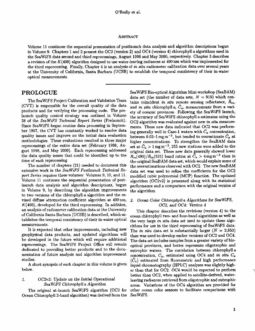
ABSTRACT

Volume II continuesthe sequentialpresentationof postlaunch data analysisand algorithm descriptionsbegun

inVolume 9.Chapters I and 2 presentthe OC2 (version2)and OC4 (version4)chlorophylla algorithmsused in

the SeaWiFS data second and thirdreprocessings,August 1998 and May 2000, respectively.Chapter 3 describes

a revisionofthe K(490) algorithmdesignedto use water-leavingradiancesat490 nm which was implemented for

the thirdreprocessing.Finally,Chapter 4 isan analysisof inhtu radiometer calibrationdata over severalyears

at the Universityof California,Santa Barbara (UCSB) to establishthe temporal consistencyof theirin-water

opticalmeasurements.

PROLOGUE

The SeaWiFS ProjectCalibrationand ValidationTeam

(CVT) isresponsiblefor the overallqualityof the data

products and forverifyingthe processingcode. The pre-

launch qualitycontrolstrategy was outlined in Volume

38 of the SeaWiFS Technical Report Series (Prelaunch).

Since SeaWiFS began routine data processing in Septem-

ber 1997, the CVT has constantly worked to resolve data

quality issues and improve on the initial data evaluation

methodologies. These evaluations resulted in three major

reprocessings of the entire data set (February 1998, Au-

gust 1998, and May 2000). Each reprocessing addressed

the data quality issues that could be identified up to the

time of each reprocessing.The number of chapters (21) needed to document this

extensive work in the SeaWiFS Postlaunch Technical Re-

port Series requires three volumes: Volumes 9, 10, and 11.Volume tl continues the sequential presentation of post-

launch data analysis and algorithm descriptions, begun

in Volume 9, by describing the algorithm improvements

to two versions of the chlorophyll a algorithm and the re-

vised diffuse attenuation coefficient algorithm at 490nm,

K(490), developed for the third reprocessing. In addition,an analysis of radiometer calibration data at the University

of California Santa Barbara (UCSB) is described, which es-tablishes the temporal consistency of their in-water opticalmeasurements.

It is expected that other improvements, including new

geophysical data products, and updated algorithms will

be developed in the future which will require additional

reprocessings. The SeaWiFS Project Office will remaindedicated to providing better products and to the docu-

mentation of future analysis and algorithm improvementstudies.

A short synopsis of each chapter in this volume is givenbelow.

1. 0C2v2: Update on the Initial Operational

SeaWiFS Chlorophyll a Algorithm

The original at-launch SeaWiFS algorithm (OC2 for

Ocean Chlorophyll 2-band algorithm) was derived from the

SeaWiFS Bio-optical Algorithm Mini-workshop (SeaBAM)

data set (the number of data sets, N = 919) which con-tains coincident in situ remote sensing reflectance, ]_,

and in situ chlorophyll a, Ca, measurements from a vari-

ety of oceanic provinces. Following the SeaWiFS launch,the accuracy of SeaWiFS chlorophyll a estimates using the

OC2 algorithm was evaluated against new in situ measure-ments. These new data indicated that OC2 was perform-

ing generally well in Case-1 waters with Ca concentration,

between 0.03-1 mgm -3, but tended to overestimate Ca at

higher concentrations. To strengthen the SeaBAM dataset at C'a > 1 mgm -3, 255 new stations were added to the

original data set. These new data _enerally showed lowerRrs(490)/Rrs(555) band ratios at Ca > 4mgm -3 than in

the original SeaBAM data set, which would explain some ofthe overestimations observed with OC2. The new SeaBAM

data set was used to refine the coefficients for the OC2

modified cubic polynomial (MCP) function. The updated

algorithm (OC2v2) is presented along with its statisticalperformance and a comparison with the original version of

the algorithm.

2. Ocean Color Chlorophyll a Algorithms for SeaWiFS,

0C2, and 0C4: Version 4

This chapter describes the revisions (version 4) to theocean chlorophyll two- and four-band algorithms as well as

the very large in situ data set used to update these algo-rithms for use in the third reprocessing of SeaWiFS data.

The in situ data set is substantially larger (N = 2,853)

than was used to develop earlier versions of OC2 and OC4.

The data set includes samples from a greater variety of bio-

optical provinces, and better represents oligotrophic and

eutrophic waters. The correlation between chlorophyll aconcentration, Ca, estimated using OC4 and in situ Ca

(Ca) estimated from fluorometric and high performance

liquid chromatography (HPLC) analyses was slightly high-er than that for OC2. OC4 would be expected to perform

better than OC2, when applied to satellite-derived, water-

leaving radiances retrieved from oligotrophic and eutrophicareas. Variations of the OC4 algorithm are provided for

other ocean color sensors to facilitate comparisons withSeaWiFS.

SeaWiFSPostlaunchCalibration and Validation Analyses, Part 3

3. SeaWiFS Algorithm for the Diffuse Attenuation

Coefficient, K(490), Using Water-LeavingRadiances at 490 and 555nm

A new algorithm has been developed using the ratio

of water-leaving radiances at 490 and 555 nm to estimate

K(490), the diffuse attenuation coefficient of seawater at490nm. The standard uncertainty of prediction for the

new algorithm is statistically identical to that of the Sea-

WiFS prelaunch K(490) algorithm, which uses the ratio

of water-leaving radiances at 443 and 490nm. The new

algorithm should be used whenever the uncertainty of theSeaWiFS determination of water-leaving radiance at 443

is larger than that at 490 nm.

4. Long-Term Calibration History of SeveralMarine Environmental Radiometers (MERs)

The accuracy of upper ocean apparent optical prop-

erties (AOPs) for the vicarious calibration of ocean color

satellites ultimately depends on accurate and consistent insitu radiometric data. The Sensor Intercomparison and

Merger for Biological and Interdisciplinary Oceanic Stud-

ies (SIMBIOS) project is charged with providing estimatesof normalized water-leaving radiance for the SeaWiFS in-strument to within 5%. This, in turn, demands that the ra-

diometric stability of in situ instruments be within 1% with

an absolute accuracy of 3%. This chapter is a report on

the analysis and reconciliation of the laboratory calibration

history for several Biospherical Instruments (BSI) marineenvironmental radiometers (MERs), models MER-2040

and -2041, three of which participate in the SeaWiFS Cal-

ibration and Validation Program. This analysis includes

data using four different FEL calibration lamps, as wellas calibrations performed at three SeaWiFS Intercalibra-

tion Round-Robin Experiments (SIRREXs). Barring a few

spectral detectors with known deteriorating responses, the

radiometers used by the University of California, Santa

Barbara (UCSB) during the Bermuda Bio-Optics Project(BBOP) have been remarkably stable during more than

five years of intense data collection. Coefficients of varia-

tion for long-term averages of calibration slopes, for most

detectors in the profiling instrument, were less than 1%.

Long-term averages can be applied to most channels, with

deviations only after major instrument upgrades. Themethods used here to examine stability accommodate the

addition of new calibration data as they become available.

This enables researchers to closely track any changes in the

performance of these instruments and to adjust the cali-

bration coefficients accordingly. This analysis may serve as

a template for radiometer histories which will be cataloged

by the SIMBIOS Project.

O'Reillyet al.

Chapter 1

OC2v2: Update on the Initial Operational

SeaWiFS Chlorophyll a Algorithm

STEPHANE MARITORENA

ICESS/University of California at Santa Barbara

Santa Barbara, California

JOHN E. O'REILLY

NOAA National Marine Fisheries Service

Narragansett, Rhode Island

ABSTRACT

The original at-launch SeaWiFS algorithm (OC2 for Ocean Chlorophyll 2-band algorithm) was derived from

the SeaBAM data set (N = 919) which contains coincident remote sensing reflectance, /}rs, and in situ chlo-rophyll a, Ca, measurements from a variety of oceanic provinces. Following the SeaWiFS launch, the accuracy

of SeaWiFS chlorophyll a estimates using the OC2 algorithm was evaluated against new in situ measurements.These new data indicated that OC2 was performing generally well in Case-1 waters with Ca concentration,

between 0.03-1 mgm -a, but tended to overestimate (_a at higher concentrations. To strengthen the SeaBAM

data set at Ca > 1 mgm -3, 255 new stations were added to the original data set. These new data generally

showed lower Rrs(490)/R,s(555) band ratios at C'a > 4mgm -3 than in the original SeaBAM data set, which

would explain some of the overestimations observed with OC2. The new SeaBAM data set was used to refine the

coefficients for the OC2 MCP function. The updated algorithm (OC2v2) is presented along with its statistical

performance and a Comparison with the original version of the algorithm.

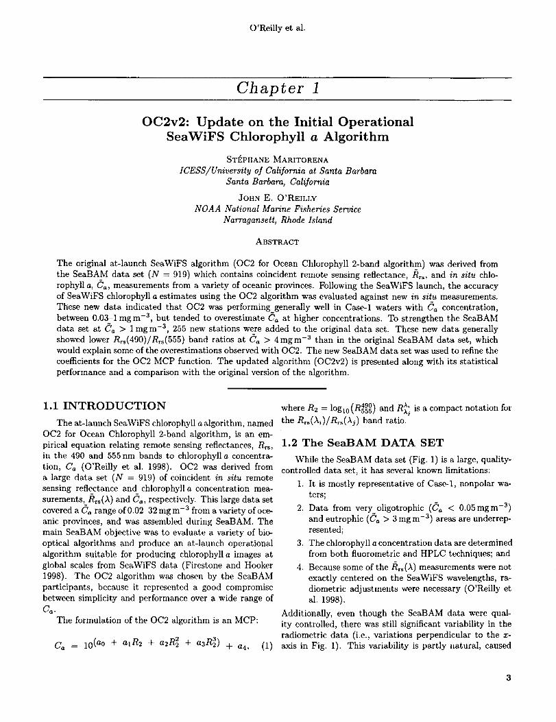
1.1 INTRODUCTION

The at-launch SeaWiFS chlorophyll a algorithm, named

OC2 for Ocean Chlorophyll 2-band algorithm, is an em-

pirical equation relating remote sensing reflectances, Rrs,

in the 490 and 555nm bands to chlorophyll a concentra-

tion, Ca (O'Reilly et al. 1998). OC2 was derived from

a large data set (N = 919) of coincident in situ remotesensing reflectance and chlorophyll a concentration mea-

surements,/)rs(A) and Ca, respectively. This large data set

covered a Ca range of 0.02-32 mg m -3 from a variety of oce-

anic provinces, and was assembled during SeaBAM. The

main SeaBAM objective was to evaluate a variety of bio-

optical algorithms and produce an at-launch operational

algorithm suitable for producing chlorophyll a images at

global scales from SeaWiFS data (Firestone and Hooker

1998). The OC2 algorithm was chosen by the SeaBAM

participants, because it represented a good compromise

between simplicity and performance over a wide range of

ca.The formulation of the OC2 algorithm is an MCP:

Ca = 10 (a° + a,R2 + a2R_ + a3 R3) + a4, (1)

490where R2 = log10(Rs55) and R_; is a compact notation for

the Rrs(A_)/Rrs(Aj) band ratio.

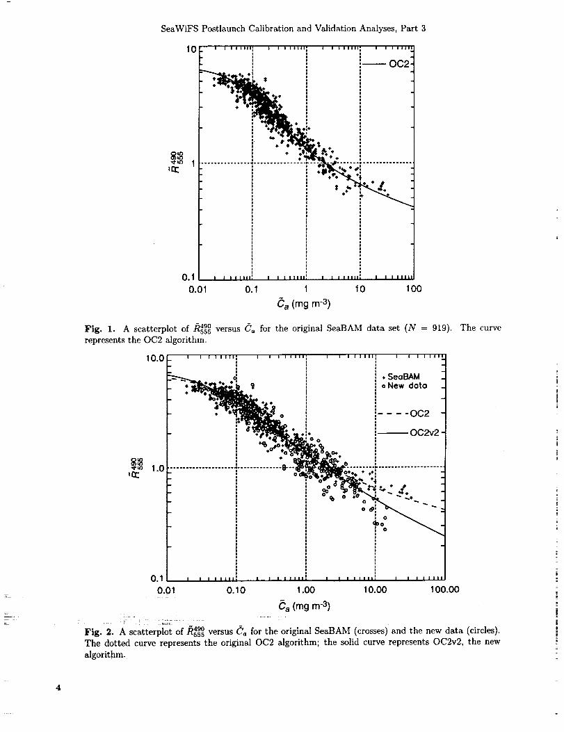
1.2 The SeaBAM DATA SET

While the SeaBAM data set (Fig. I) is a large, quality-controlled data set, it has several known limitations:

1. It is mostly representative of Case-l, nonpolar wa-

ters;

2. Data from very oligotrophic (Ca < 0-05mg m-3)

and eutrophic (Ca > 3 mg m -3) areas are underrep-

resented;

3. The chlorophyll a concentration data are determined

from both fluorometric and HPLC techniques; and

4. Because some of the/_rs(A) measurements were not

exactly centered on the SeaWiFS wavelengths, ra-

diometric adjustments were necessary (O'Reilly et

al. 1998).

Additionally, even though the SeaBAM data were qual-

ity controlled, there was still significant variability in the

radiometric data (i.e., variations perpendicular to the x-

axis in Fig. 1). This variability is partly natural, caused

3

SeaWiFSPostlaunchCalibrationandValidationAnalyses,Part3

10

0.1

0.0

I I I l 1111 I I I iOIli I I I Illll I I I I IIII

,-- 0C2-"

" % ÷ .i ÷

...... -*--_--_-.;"...... i...............

*.':"_...

I I I IIIIh I I I I lllll I• I I 1 IIII1_ I I I Illl

0.1 1 10 100

Ca (mg m -3)

Fig. 1. A scatterplot of 5490 Ca for the original SeaBAM data set (N = 919).• _555 versus

represents the OC2 algorithm

10.0 __,__.jL'.'.' '''",..d, 9' ' ' '''" ' ' ''''" o'NewSeaBAM''dato'.... .:'

i .... 0C2 -

__ "_.:. i_ oc_2 -"+__ _,

............. _-__- ........ . .....................--_o%-_-_..;

o.,I.....,,,, .......:,,,....10.01 O. 10 10.00 100.00

I I I I'::: l

1.00

_ (rag m-3)

The curve

Fig. 2. A scatterplot of 549o"'sss versus Ca for the original SeaBAM (crosses) and the new data (circles).

The dotted curve represents the original OC2 algorithm; the solid curve represents OC2v2, the new

algorithm.

4

O'Reflly et al.

1oo__pE:, REDUCEb'M'_OR:AXIS'._....F N:, 1174 .'_ / :r- INT: -0,0000 .-'" + 7 "i" S=I2OPE; !.0000 ..'" +# v" ,:

lOk-_r_i_._ .......... :,.--_--.,-,,:+-d-----.,.-.-::-_

•. ....,]it L .

o.,:J:

0.01 ..... "..... , .....................0.01 0.1 1 10 100

ca (_g rl)

1°°I,--, 10

°m4.*

t-(0

O

0.1

0.010.01

, , ,,,,,o , . ,,,,,, , , ,,,,,, ,: ,,,,.

i i iiiiii i i iiiiii i i IIIIH i i iiiii

0.1 1 10 100

Ca Quantiles (_g 1-1)

170

153

136

119

_., 102

85

¢.51

34

17

0-1.00

N: 1174MIN: -0.753MAX: 0.872MED: -0.003MEAN: -0.000STD: 0.196SKEW: 0°034KURT: 1.511

-0.75 -0.50 -0.25 0.00 0.25

I°g(Ca �Ca )

0.50 0.75 1.00 0.01

I

_,11_ _11 _11111 i i willn _ r r_TTVln

N= 1174

--%

d)

0.1 1 10 100

ca (_g,-1)

100

10

I

o) 1

0.1

0.010.1 1.0 10.0

• __._t ¸¸ :..

+÷ e)++-_____

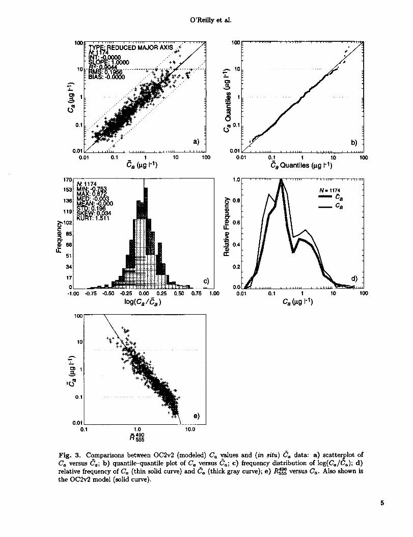
Fig. 3. Comparisons between OC2v2 (modeled) Ca values and (in situ) Ca data: a) scatterplot of

Ca versus Ca; b) quantile-quantile plot of Ca versus Ca; c) frequency distribution of log(Ca/Ca); d)

relative frequency of Ca (thin solid curve) and Ca (thick gray curve); e) Rsss49°versus Ca. Also shown is

the OC2v2 model (solid curve).

SeaWiFS Postlaunch Calibration and Validation Analyses, Part 3

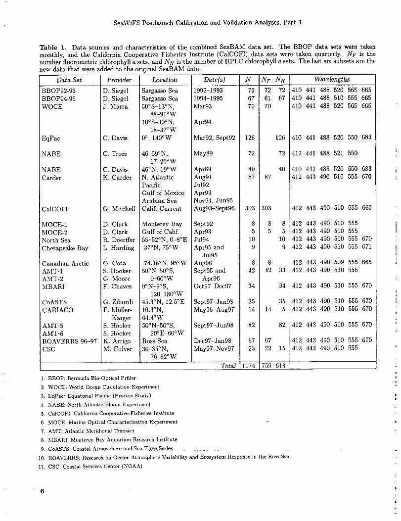
Table 1. Data sources and characteristics of the combined SeaBAM data set. The BBOP data sets were taken

monthly, and the California Cooperative Fisheries Institute (CalCOFI) data sets were taken quarterly. NF is thenumber fluorometric chlorophyll a sets, and NH is the number of HPLC chlorophyll a sets. The last six subsets are the

new data that were added to the original SeaBAM data.

BBOP92-93

BBOP94-95

WOCE

EqPac

NABE

NABE

Carder

CalCOFI

MOCE-1

MOCE-2

North Sea

Chesapeake Bay

Canadian Arctic

AMT-1AMT-2

MBARI

Data Set Provider Location Date(s)

D. Siegel

COASTS

CARIACO

D. SiegelJ. Marra

:C. Davis

C. Trees

IC. Davis

K. Carder

G. Mitchell

D. Clark

D. Clark

R. Doerffer

L. Harding

G. Cota

S. Hooker

G. Moore

F. Chavez

G. Zibordi

F. Miiller-

KargerS. Hooker

S. Hooker

K. ArrigoM. Culver

AMT-5

AMT-6ROAVERRS 96-97

CSC

Sargasso Sea

Sargasso Sea50°S-13°N,

88 91°W

10°S-30°N,18-37°W

0°, 140°W

46-59°N,17-200W

46°N, 19°WN. Atlantic

Pacific

Gulf of Mexico

Arabian Sea

Calif. Current

Monterey BayGulf of Calif.

55-52°N, 0-8°E

37°N, 75°W

74.38°N, 95°W

50°N-50°S,0-60°W

9°N-9°S,120-180°W

45.3°N, 12.5°E

10.3°N,64.4°W

50°N-50°S,20°E-60°W

Ross Sea

30-35°N,76-82°W

N

1992-1993 72 72 72

1994-1995 67 61 67

Mar93 70 70

Apr94

Mar92, Sept92

May89

Apt89

Aug91Ju192

Apr93Nov94, Jun95

Aug93-Sept96

NF NH Wavelengths

:4i'() 441 488 520 565 665

t26 126

72 72

40 40

87 87

303 303

Sept92 8 8 8

Apt93 5 5 5Jul94 10 10

Apr95 and 9 9Ju195

Aug96 8 8

Sept95 and 42 42 33

Apt96Oct97-Dec97 34 34

Sept97-Jan98 35 35

May96-Aug97 14 14 5

Sept97-Jun98 82 82

Dec97-Jan98 67 67

May97-Nov97 23 22 15

Total 1174 759 613

1. BBOP: Bermuda Bio-Optical Prfiler

2. WOCE: World Ocean Circulation Experiment

3. EqPac: Equatorial Pacific (Process Study)

4. NABE: North Atlantic Bloom Experiment

5. CaICOFI: California Cooperative Fisheries Institute

6. MOCE: Marine Optical Characterization Experiment

7. AMT: Atlantic Meridional Transect

8. MBARI: Monterey Bay Aquarium Research Institute

9. COASTS: Coastal Atmosphere and Sea Time Series ....

10. ROAVERRS: Research on Ocean-Atmosphere Variability and Ecosystem Response in the Ross Sea

11. CSC: Coastal Services Center (NOAA)

410 441 488 510 555 665

410 441 488 520 565 665

410 441 488 520 550 683

412 441 488 521 550

410 441 488 520 550 683

412 443 490 510 555 670

412 443 490 510 555 665

412 443 490 510 555i

!412 443 490 510 555i

]412 443 490 510 555 670

412 443 490 510 555 671

412 443 490 509 555 665

412 443 490 510 555

412 443 490 510 555 670

412 443 490 510 555 670

412 443 490 510 555 670

412 443 490 510 555 670

412 443 490 510 555 670

412 443 490 510 555

O'Reillyet al.

_00 ,' i I I lllll i I I B III I I I i IIII I / I I I Ill

" 0 ........................................... 2I

g

0.01 , , ,LA ,,' , , '''_H' , _ ,,,,,,; i , _i,,'

0.01 0.1 I 10 100

initialAlgorithm Ca (rag m -3)

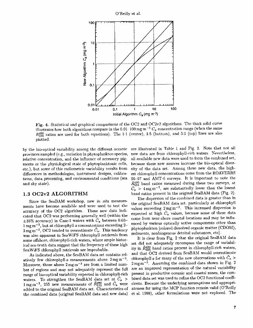
Fig. 4. Statistical and graphical comparisons of the OC2 and OC2v2 algorithms. The thick solid curve

illustrates how both algorithms compare in the 0.01-100 mg m -3 Ca concentration range (when the same

R490 ratios are used for both equations). The 1:1 (center), 1:5 (bottom), and 5:1 (top) lines are also555

plotted.

by the bio-optical variability among the different oceanicprovinces sampled (e.g., variation in phytoplankton species,

relative concentration, and the influence of accessory pig-

ments or the physiological state of phytoplanktonic cells,

etc.), but some of this radiometric variability results fromdifferences in methodologies, instrument designs, calibra-

tions, data processing, and environmental conditions (sea

and sky state).

1.3 OC2v2 ALGORITHM

Since the SeaBAM workshop, new in situ measure-ments have become available and were used to test the

accuracy of the OC2 algorithm. These new data indi-

cated that OC2 was performing generally well (within the+35% accuracy) in Case-1 waters with Ca between 0.03-

1 mgm -3, but at chlorophyll a concentrations exceeding 2-

3mgm -3, OC2 tended to overestimate (_a. This tendency

was also apparent in SeaWiFS chlorophyll retrievals fromsome offshore, chlorophyll-rich waters, where ample histor-

ical sea-truth data suggest that the frequency of these highSeaWiFS chlorophyll retrievals are improbable.

As indicated above, the SeaBAM data set contains rel-

atively few chlorophyll a measurements above 2mgm -3.

Moreover, those above 2 mg m -3 are from a limited num-

ber of regions and may not adequately represent the fullrange of bio-optical variability expected in chlorophyll-rich

waters. To strengthen the SeaBAM data set at Ca >l mgm -3, 255 new measurements of flag0 and Ca were

"_555

added to the original SeaBAM data set. Characteristics of

the combined data (original SeaBAM data and new data)

are illustrated in Table 1 and Fig. 2. Note that not all

new data are from chlorophyll-rich waters. Nevertheless,

all available new data were used to form the combined set,

because these new sources increase the bio-optical diver-

sity of the data set. Among these new data, the high-

est chlorophyll concentrations come from the ROAVERRS

96-97 and AMT-6 surveys. It is important to note theR'490 band ratios measured during these two surveys, at

555

Ca > 4mgm -3, are substantially lower than the lowest

band ratios present in the original SeaBAM data (Fig. 2).

The dispersion of the combined data is greater than in

the original SeaBAM data set, particularly at chlorophyll

values exceeding 2 mgm -3. This increased dispersion isexpected at high Ca values, because some of these data

come from near-shore coastal locations and may be influ-

enced by various optically active components other than

phytoplankton [colored dissolved organic matter (CDOM),

sediments, nonbiogenous detrital substances, etc].

It is clear from Fig. 2 that the original SeaBAM data

set did not adequately encompass the range of variabil-

ity in h_ 9° band ratios present in chlorophyll-rich waters,and that OC2 derived from SeaBAM would overestimate

chlorophyll a for many of the new observations with Ca >

2mgm -3. Assuming the combined data shown in Fig. 2

are an improved representation of the natural variability

present in productive oceanic and coastal zones, the com-bined data set was used to refine the OC2 functional coeffi-

cients. Because the underlying assumptions and appropri-

ateness for using the MCP function remain valid (O'Reilly

et al. 1998), other formulations were not explored. The

SeaWiFS Postlaunch Calibrationand ValidationAnalyses,Part 3

updated algorithm (OC2v2) isas follows:

U. = 10 (0.2974 - 2.2429R2 + 0.8358P_ - 0.0077/_) _ 0.0929 (2)

where R2 is defined as in (1).Statistical and graphical comparisons between chloro-

phyll a concentrations derived from OC2v2 versus Ca are

presented in Fig. 3. A comparison of the output from

OC2 and OC2v2 is illustrated in Fig. 4. OC2 and OC2v2

yield very similar results for Co ranging between 0.03-

1.5mgm -3. At chlorophyll a values exceeding 3mgm -s,

OC2v2 estimates are substantially lower than OC2. At

very low chlorophyll a concentrations, 0.01-0.02 mg m -3,

OC2v2 produces slightly higher concentrations than 0C2.

limitationsof the originalSeaBAM data set remain valid

for the new combined data. More good quality]_rs(A)

and U, data are needed from regionswith chlorophylla

concentrationsabove 3.0 and below 0.04mg m -3 to better

characterizethe bio-opticalvariabilityofthesewaters and,

thus,to identifypotentialstrategiesto achievereasonable

satellitechlorophylla retrievals.

ACKNOWLEDGMENTS

1.4 CONCLUSIONS

While, on average,OC2v2, should resultinan improve-

ment over OC2 inchlorophyll-richareas,the uncertainties

remain largeforC',> 3-4 mg m -3. Itmust be emphasized

that because the variabilityof the data increasesat high

concentrations,the precisionof the SeaWiFS retrievalsis

inevitablydegraded. Itmust alsobe kept inmind that the

The authorswish to thank allthe participantsofthe SeaBAMworkshop fortheirhelpand contributionto thedata set:K.L.Carder,S.A. Garver,S.K. Hawes, M. Kahru, C.R. McClain,

B.G. Mitchell,G.F. Moore, J.L.Mue!ler,B.D. Schi'eber,andD.A. Siegel.We alsowould liketoacknowledgeJ.Aiken,K.R.Arrigo,F.P.Chavez,D.K. Clark,G.F. Cot°,M.E. Culver,C.O.Davis,R. Doerffer,L.W. Harding,S.B.Hooker,J.Marra, F.E.

Mfiller-Karger,A. Subramaniam, C.C. Trees,and G. Zibordiwho kindlyprovidedsome oftheirdata.

8

O'Reilly et al.

Chapter 2

Ocean Color Chlorophyll a Algorithms for

SeaWiFS, OC2, and OC4: Version 4

JOHN E. O'REILLY

NOAA, National Marine Fisheries Service, Narragansett, Rhode Island

STEPHANE MARITORENA, DAVID A. SIEGEL, MARGARET C. O'BRIEN, AND DIERDRE TOOLE

ICESS/University of California Santa Barbara, Santa Barbara, California

B. GREG MITCHELL AND MATI KAHRU

Scripps Institution of Oceanography, University of California, San Diego, California

FRANCISCO P. CHAVEZ AND P. STRUTTON

Monterey Bay Aquarium Research Institute, Moss Landing, California

GLENN F. COTA

Old Dominion University, Norfolk, Virginia

STANFORD B. HOOKER AND CHARLES R. MCCLAIN

NASA Goddard Space Flight Center, Greenbelt, Maryland

KENDALL L. CARDER AND FRANK MOLLER-KARGER

University of South Florida, St. Petersburg, Florida

LARRY HARDING AND ANDREA MAGNUSON

Horn Point Laboratory, University of Maryland, Cambridge, Maryland

DAVID PHINNEY

Bigelow Laboratory for Ocean Sciences, West Boothbay Harbor, Maine

GERALD F. MOORE AND JAMES AIKEN

Plymouth Marine Laboratory, Plymouth, United Kingdom

KEVIN R. ARRIGO

Department of Geophysics, Stanford University, Stanford, California

RICARDO LETELIER

College of Oceanic and Atmospheric Sciences, Oregon State University

MARY CULVER

NOAA, Coastal Services Center, Charleston, South Carolina

ABSTRACT

This chapterdescribesthe revisions(version4) to the ocean chlorophylltwo- and four-band algorithms,as well

as the very largein situdata setused to update these algorithms foruse in the thirdreprocessingofSeaWiFS

data. The in situdata set issubstantiallylarger(N = 2,853)than was used to develop earlierversionsofOC2

and OC4. The data set includessamples from a greatervarietyofbio-opticalprovinces,and betterrepresents

oligotrophicand eutrophic waters. The correlationbetween chlorophylla concentration,Ca, estimated usingOC4 and in situCa (Ca) estimated from fluorometricand HPLC analyses was slightlyhigher than that for

OC2. OC4 would be expected to perform betterthan OC2, when applied to satellite-derived,water-leavlng

radiances retrievedfrom oligotrophicand eutrophic areas. Variationsof the OC4 algorithm are provided for

other ocean colorsensorsto facilitatecomparisons with SeaWiFS.

SeaWiFS Postlaunch Calibration and Validation Analyses, Part 3

2.1 INTRODUCTION

The accuracy, precision, and utility of an empirical

ocean color algorithm for estimating global chlorophyll a

distributions depends on the characteristics of the algo-

rithm and the in situ observations used to develop it. The

empirical pigment and chlorophyll algorithm widely used

in the processing of the global Coastal Zone Color Scan-

ner (CZCS) data set was developed using fewer than 60

in situ radiance and chlorophyll a pigment observations

(Evans and Gordon 1994). Since the CZCS period, a num-

ber of investigators have measured in situ remote sensingreflectance, Rrs(,k), and in situ chlorophyll a concentra-tion, Ca, from a variety of oceanic provinces. In 1997, the

SeaBAM group (Firestone and Hooker 1998) assembled a

large Rrs(A) and Ca data set containing 919 observations.This data set was used to evaluate the statistical perfor-

mance of chlorophyll a algorithms and to develop the ocean

chlorophyll 2-band (OC2) and ocean chlorophyll 4-band

(OC4) algorithms (O'Reilly et al. 1998).

OC2 predicts Ca from the Rrs(490)/Rrs(555) band ratio

using an MCP formulation. Hereafter, the Rr_ ratio con-structed from band A divided by band B is indicated by

R_, i.e., the Rrs(490)/Rrs(555) band ratio is representedby _490 OC4 also relates band ratios to chlorophyll a with• _555"

a single polynomial function, but it uses the maximum

band ratio (MBR) determined as the greater of the _443_555,

R49o _51o values. OC2 was employed as the standard555, Or _555

chlorophyll a algorithm by the SeaWiFS Project followingthe launch of SeaWiFS in September 1997. Although the

statistical characteristics of OC4 were superior to those of

OC2, the SeaBAM group recommended using the simpler2-band OC2 at launch.

With the goal of improving estimates in chlorophyll-

rich waters, OC2 was revised (version 2) based on an ex-

panded data set of 1,174 in situ observations (Maritorena

and O'Reilly 2000) and applied by the SeaWiFS Project inthe second data reprocessing (McClain 2000). Additional

in situ data have become available as the result of new pro-

grams (e.g., SIMBIOS) and the continuation and expan-sion of ongoing field campaigns. These new data increase

the variety of bio-optical provinces represented in the origi-

nal data set and fill in regions of the Rr_(A) and Ca domain

which were not previously well represented. Also, results

from over 2.5 years of SeaWiFS data are now available to

assess the overall performance of the SeaWiFS instrument

2.2 THE IN SITU DATA SET

A very large data set of/_rs(_) and Ca measurements

were assembled for the purpose of updating ocean color

chlorophyll algorithms for SeaWiFS calibration and vali-

dation activities. The data sets and the principal investi-

gators responsible for collecting the data are provided in

Table 2. Table 3 gives the location and acquisition time pe-

riods of the data, along with an indication of the number

of observations, how the chlorophyll a concentration was

determined (fluorometry or HPLC), and how the radio-

metric observations were made (above- or in-water). The

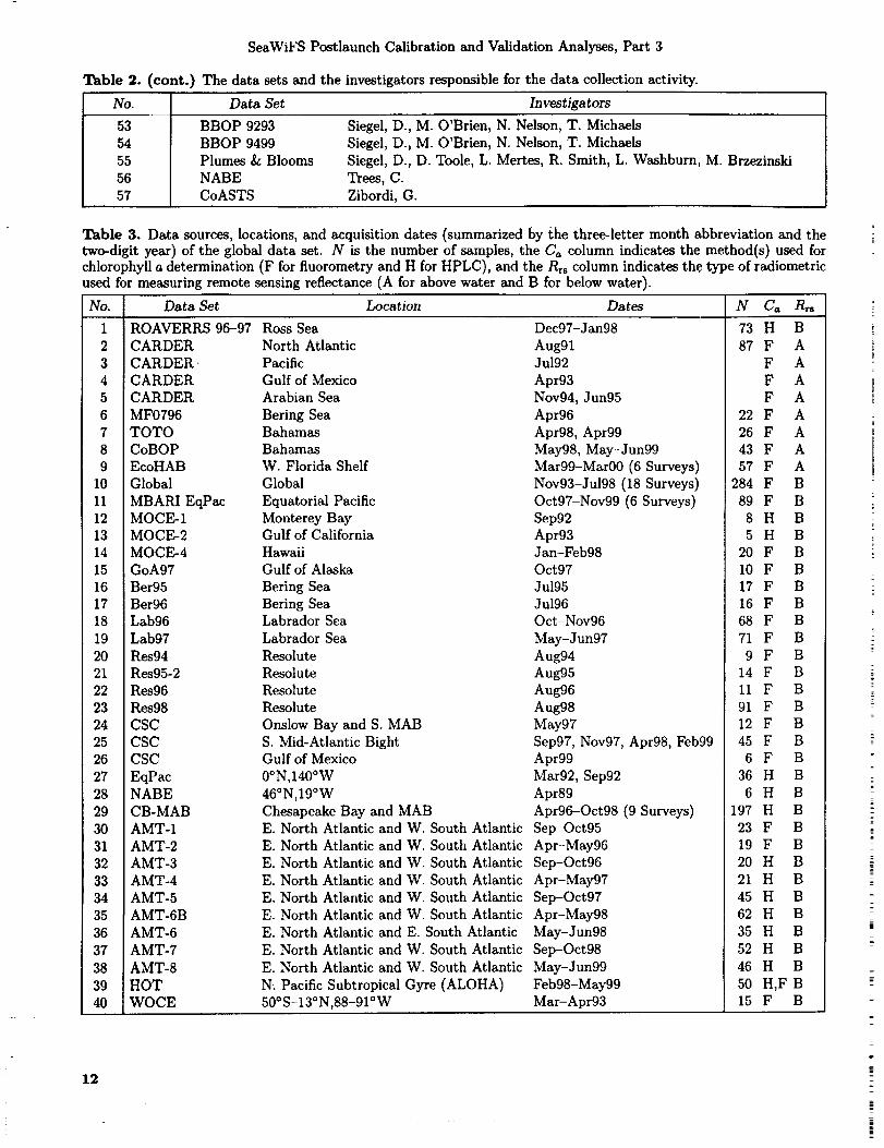
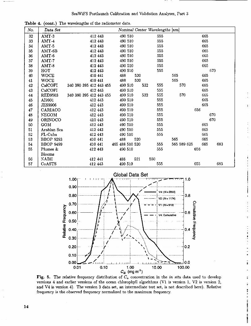
wavelengths of the latter are presented in Table 4.The data set has a total of 2,853 in situ observations. It

is the largest ever assembled for algorithm refinement, and

represents a large diversity of bio-optical provinces. The

Ca data are derived from a mixture of HPLC and fluoro-

metric measurements from surface samples: 28% and 72%

of the data, respectively (Table 3). The Ca values range

from 0.008-90 mg m -3. The relative frequency distribution

of Ca has a primary and secondary peak at 0.2mgm -3

and approximately l mgm -3, respectively (Fig. 5). Oce-

anic regions with Ca between 0.08-3 mg m -3 are relatively

well represented. There are 238 observations of Ca ex-

ceeding 5mgm -3 and 116 observations with Ca less than

0.05mgm -3. A comparison of the Ca frequency distri-

bution with those from previous versions (O'Reilly et al.

1998 and Maritorena and O'Reilly 2000) shows that. olig-

otrophic and eutrophic waters are relatively better repre-sented in the current data set. The present data set also

has a more equitable distribution over a broader range of

Ca (i.e., 0.08-3mgm-3).

Measurements of RCs(),) were made using both above-and in-water radiometers: 88% and 12% of the data, re-

spectively (Table 3). In several subsets, multiple R_s mea-surements were taken at stations where only a single Ca

measurement was made. For these subsets (BBOP9293,

WOCE, EqPac, NABE, GoA97, Ber96, Bet95, Lab97,

Lab96, Res96, Res95-2, Res94), the median Rrs value was

paired with the solitary Ca observation and added to thedata set.

Except in a limited number of circumstances, band ra-

tios determined from the median Rrs values agreed well

with the individual band ratios. Several subsets, however,

required adjustments to the/_()_) values to conform with

and identify areas where improvements are needed in the the SeaWiFS band set. The R_(555) value was estimated

processing of satellite ocean color data (McClain 2000). from the /_rs(565) measurement for the BBOP9293 and

An update to the OC2 and OC4 chlorophyll algorithms WOCE data using an equation derived from concurrent

for SeaWiFS are presented in this chapter, along with a

description of the major features of the very large in situdata set used to refine these models, and a comparison of

the updated algorithms with earlier versions_ MBR chloro-

phyll algorithms for several other satellite ocean color sen-sors are also provided to facilitate intercomparisons withSeaWiFS.

measurements of /_rs(555) and /_rs(565) from 1994-1995

BBOP surveys (equation 2 from O'Reilly et al. 1998). TheRr_(555) value for the CB-MAB subset was computed by

averaging the/_rs(550) and/_rs(560) values. The/_rs(510)value was estimated from the Rrs(520) values for the Eq-

Pac, WOCE, NABE, and BBOP9293 data sets using the

following conversion equation based on Morel and Maritor-

10

O'Reillyet al.

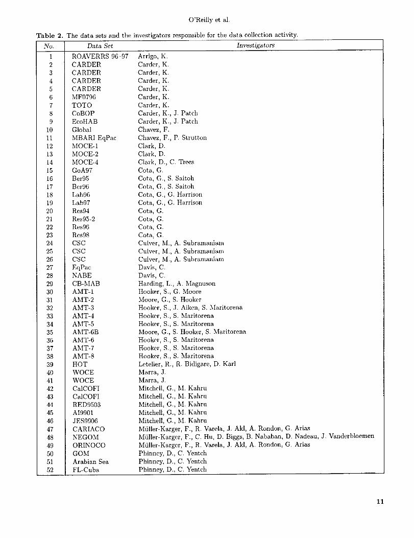
Table 2. Thedatasetsandtheinvestigatorsresponsibleforthedatacollectionactivity.No. Data Set Investigators

1 ROAVERRS 96-97

2 CARDER3 CARDER

4 CARDER

5 CARDER

6 MF0796

7 TOTO8 CoBOP

9 EcoHAB

10 Global

11 MBARI EqPac12 MOCE-1

13 MOCE-2

14 MOCE-4

15 GoA97

16 Ber95

17 Bet96

18 Lab96

19 Lab97

20 Res94

21 Res95-222 Res96

23 Res98

24 CSC

25 CSC

26 CSC

27 EqPac28 NABE

29 CB-MAB

3O AMT-1

31 AMT-2

32 AMT-3

33 AMT-4

34 AMT-535 AMT-6B

36 AMT-6

37 AMT-7

38 AMT-8

39 HOT

40 WOCE

41 WOCE

42 CalCOFI43 CalCOFI

44 RED9503

45 AI9901

46 JES9906

47 CARIACO

48 NEGOM

49 ORINOCO

50 GOIvI

51 Arabian Sea

52 FL-Cuba

Arrigo, K.

Carder, K.

Carder, K.

Carder, K.

Carder, K.

Carder, K.

Carder, K.

Carder, K., J. Patch

Carder, K., J. Patch

Chavez, F.

Chavez, F., P. Strutton

Clark, D.

Clark, D.

Clark, D., C. Trees

Cota, G.

Cota, G., S. Saitoh

Cota, G., S. Saitoh

Cota, G., G. Harrison

Cota, G., G. Harrison

Cota, G.

Cota, G.Cota, G.

Cota, G.

Culver, M., A. Subramaniam

Culver, M., A. Subramaniam

Culver, M., A. Subramaniam

Davis, C.

Davis, C.

Harding, L., A. MagnusonHooker, S., G. Moore

Moore, G., S. Hooker

Hooker, S., J. Aiken, S. Maritorena

Hooker, S., S. Maritorena

Hooker, S., S. Maritorena

Moore, G., S. Hooker, S. Maritorena

Hooker, S., S. Maritorena

Hooker, S., S. Maritorena

Hooker, S., S. MaritorenaLetelier, R., R. Bidigare, D. Karl

Marra, J.

Marra, J.

Mitchell, G., M. Kahru

Mitchell, G., M. Kahru

Mitchell, G., M. Kahru

Mitchell, G., M. Kahru

Mitchell, G., M. Kahru

M/iller-Karger, F., R. Varela, J. Akl, A. Rondon, G. Arias

M/iller-Karger, F., C. Hu, D. Biggs, B. Nababan, D. Nadeau, J. Vanderbloemen

M/iller-Karger, F., R. Varela, J. Akl, A. Rondon, G. Arias

Phinney, D., C. Yentch

Phinney, D., C. Yentch

Phinney, D., C. Yentch

11

SeaWiFS Postlaunch Calibration and Validation Analyses, Part 3

Table 2. (cont.) The data sets and the investigators responsible for the data collection activity.

No. Data Set Investigators

5354

55

56

57

BBOP 9293BBOP 9499

Plumes & Blooms

NABE

COASTS

Siegel, D., M. O'Brien, N. Nelson, T. Michaels

Siegel, D., M. O'Brien, N. Nelson, T. Michaels

Siegel, D., D. Toole, L. Mertes, R. Smith, L. Washburn, M. Brzezinski

Trees, C.

Zibordi, G.

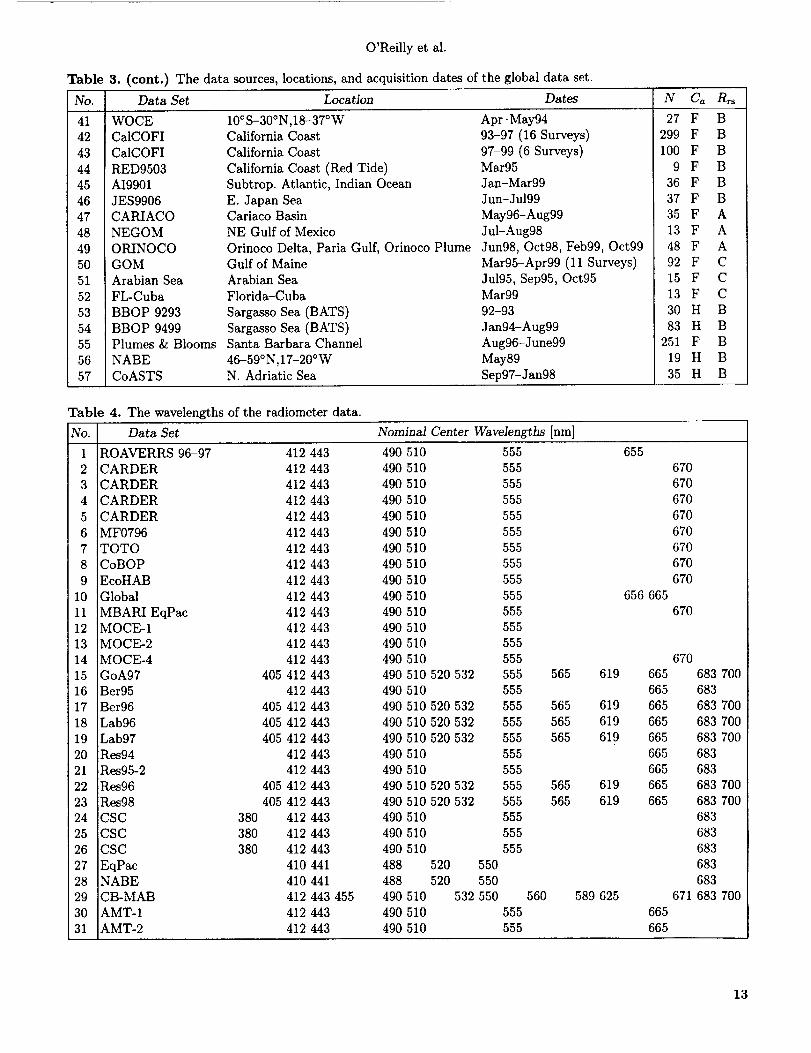
Table 3. Data sources, locations, and acquisition dates (summarized by the three-letter month abbreviation and the

two-digit year) of the global data set. N is the number of samples, the Ca column indicates the method(s) used forchlorophyll a determination (F for fluorometry and H for HPLC), and the R¢8 column indicates the type of radiometricused for measuring remote sensing reflectance (A for above water and B for below water).

Data Set Location Dates N Ca RrsNo.

1 ROAVERRS 96--97 Ross Sea Dec97-Jan98

2 CARDER North Atlantic Aug913 CARDER. Pacific Jul92

4 CARDER Gulf of Mexico Apr93

5 CARDER Arabian Sea Nov94, Jun95

6 MF0796 Bering Sea Apr96

7 TOTO Bahamas Apr98, Apr99

8 CoBOP Bahamas May98, May-Jun99

9 EcoHAB W. Florida Shelf Mar99-Mar00 (6 Surveys)

10 Global Global Nov93-Ju198 (18 Surveys)11 MBARI EqPac Equatorial Pacific Oct97-Nov99 (6 Surveys)

12 MOCE-1 Monterey Bay Sep92

13 MOCE-2 Gulf of California Apr9314 MOCE-4 Hawaii Jan-Feb98

15 GoA97 Gulf of Alaska Oct97

16 Ber95 Bering Sea Ju195

17 Ber96 Bering Sea Ju19618 Lab96 Labrador Sea Oct-Nov96

19 Lab97 Labrador Sea May-Jun97

20 Res94 Resolute Aug94

21 Res95-2 Resolute Aug95

22 Res96 Resolute Aug96

23 Res98 Resolute Aug9824 CSC Onslow Bay and S. MAB May97

25 CSC S. Mid-Atlantic Bight Sep97, Nov97, Apr98, Feb99

26 CSC Gulf of Mexico Apr99

27 EqPac 0°N,140°W Mar92, Sep92

28 NABE 46°N,19°W Apt89

29 CB-MAB Chesapeake Bay and MAB Apr96--Oct98 (9 Surveys)

30 AMT-I E. North Atlantic and W. South Atlantic Sep-Oct95

31 AMT-2 E. North Atlantic and W. South Atlantic Apt-May96

32 AMT-3 E. North Atlantic and W. South Atlantic Sep-Oct96

33 AMT-4 E. North Atlantic and W. South Atlantic Apt-May97

34 AMT-5 E. North Atlantic and W. South Atlantic Sep-Oct9735 AMT-6B E. North Atlantic and W. South Atlantic Apr-May98

36 AMT-6 E. North Atlantic and E. South Atlantic May-Jun9837 AMT-7 E. North Atlantic and W. South Atlantic Sep-Oct98

38 AMT-8 E. North Atlantic and W. South Atlantic May-Jun99

39 HOT N. Pacific Subtropical Gyre (ALOHA) Feb98-May99

40 WOCE 50°S-13°N,88-91°W Mar-Apr93

73 H B

87 F A

F A

F A

F A22 F A

26 F A

43 F A

57 F A

284 F B

89 F B

8 H B

5 H B20 F B

I0 F B

17 F B

16 F B68 F B

71 F B

9 F B

14 F B

11 F B

91 F B

12 F B45 F B

6 F B

36 H B

6 H B

197 H B

23 F B

19 F B

20 H B

21 H B

45 H B

62 H B

35 H B

52 H B

46 H B

5O H,F B15 F B

12

O'Reillyet al.

Table 3. (cont.) The data sources, locations, and acquisition dates of the global data set.

Data Set Location Dates N Ca RrsNo.

41 WOCE42 CaICOFI

43 CaICOFI

44 RED950345 AI9901

46 JES990647 CARIACO

48 NEGOM

49 ORINOCO

50 GOM51 Arabian Sea

52 FL-Cuba

53 BBOP 9293

54 BBOP 9499

55 Plumes & Blooms

56 NABE

57 COASTS

10°S-30°N,18-37°WCalifornia Coast

California Coast

California Coast (Red Tide)

Subtrop. Atlantic, Indian Ocean

E. Japan SeaCariaco Basin

NE Gulf of Mexico

Apt-May9493-97 (16 Surveys)

97-99 (6 Surveys)Mar95

Jan-Mar99

Jun-Ju199

May96-Aug99

Jul-Aug98

Orinoco Delta, Paria Gulf, Orinoco Plume Jun98, Oct98, Feb99, Oct99Gulf of Maine

Arabian Sea

Florida-Cuba

Sargasso Sea (BATS)

Sargasso Sea (BATS)Santa Barbara Channel

46-59°N,17-20°WN. Adriatic Sea

Mar95-Apr99 (11 Surveys)

Ju195, Sep95, Oct95Mar99

92-93

Jan94-Aug99

Aug96-June99

May89

Sep97-Jan98

27 F B299 F B

100 F B

9 F B

36 F B

37 F B35 F A

13 F A

48 F A92 F C

15 F C

13 F C

30 H B

83 H B

251 F B

19 H B

35 H B

Table 4. The wavelengths of the radiometer data.

No. Data Set Nominal Center Wavelengths [nm]

1 ROAVERRS 96-97 412 443

2 CARDER 412 443

3 CARDER 412 443

4 CARDER 412 443

5 CARDER 412 443

6 MF0796 412 443

7 TOTO 412 443

8 CoBOP 412 443

9 EcoHAB 412 443

10 Global 412 443

11 MBARI EqPac 412 44312 MOCE-1 412 443

13 MOCE-2 412 44314 MOCE-4 412 443

15 GoA97 405 412 443

16 Ber95 412 443

17 Ber96 405 412 443

18 Lab96 405 412 443

19 Lab97 405 412 443

20 Res94 412 443

21 Res95-2 412 443

22 Res96 405 412 443

23 Res98 405 412 443

24 CSC 380 412 44325 CSC 380 412 443

26 CSC 380 412 443

27 EqPac 410 44128 NABE 410 441

29 CB-MAB 412 443

30 AMT-1 412 443

31 AMT-2 412 443

455

490 510 555

490 510 555

490 510 555

490510 555

490510 555

490 510 555

490510 555

490 510 555

490 510 555

490 510 555

490 510 555

490 510 555

490 510 555

490 510 555

490 510 520 532 555

490 510 555

490 510 520 532 555

490 510 520 532 555

490 510 520 532 555

490 510 555490 510 555

490 510 520 532 555

490 510 520 532 555

490 510 555

490 510 555

490 510 555

488 520 550

488 520 550

490 510 532 550

490 510 555

490 510 555

560

655

656 665

565 619 665

665

565 619 665

565 619 665

565 619 665

665

665

565 619 665

565 619 665

589 625

665

665

670

670

670

670

670

670

670

670

670

670683 700

683

683 700

683 700

683 700

683

683

683 700

683 700683

683

683

683

683

671 683 700

13

SeaWiFSPostlaunchCalibrationandValidationAnalyses,Part3

Table4. (cont.) The wavelengths of the radiometer data.

No.

32 AMT-3 412 443 490 510

33 AMT-4 412 443 490 510

34 AMT-5 412 443 490 510

35 AMT-6B 412 443 490 510

36 AMT-6 412 443 490 510

37 AMT-7 412 443 490 510

38 AMT-8 412 443 490 510

39 HOT 412 443 490 510

40 WOCE 410 441 488 520

41 WOCE 410 441 488 520

42 CalCOFI 340 380 395 412 443 455 490 510

43 CalCOFI 412 443 490 510

44 RED9503 340 380 395 412 443 455 490 510

45 AI9901 412 443 490 510

46 JES9906 412 443 490 510

47 CARIACO 412 443 490 510

48 NEGOM 412 443 490 510

49 ORINOCO 410 443 490 510

50 GOM 412 443 490 510

51 Arabian Sea 412 443 490 51052 FL-Cuba 412 443 490 510

53 BBOP 9293 410 441 488 520

54 BBOP 9499 410 441 465 488 510 520

55 Plumes & 412 443 490 510

Blooms

56 NABE 412 441 488 521

57 COASTS 412 443 490 510

Data Set Nominal Center Wavelengths [nm]

532

532

555

555

555

555

555

555

555

555

665

665

665

665

665

665

665

565 665

565 665

570 665

665570 665

665

665

656

670

555

555

555555

555

555

555555

555 665

555 665

555 665

565 665

555 565 589 625 665 683

555 656

670

670

550555 655 683

14

Global Data Set

0.90 .................... _ I

o.8o .....................................i ............_ :-:::::::::Tv_;i;,:ii_;;............- 0.8! ;:7 i , J o

0.60 i ,'i I_.= 1; _\_ ........_ - -.!v4;_mu,.,_. 0.6 E

o0o ti; \ ,$

n- 0.30

0.20 ..................i.......... iO. 2

/_: :IV'. :\ -

0.10 .........._ ..-_7-- i.............................................i ................................'_' ':" _!_::_ ....................:0.00 _.,,_ ..-- ," ..... _ , , ,l[l,_ ......... ";=';";" ,_',_, 0.0

0.01 0.10 1.00 10.00 100.00C a (mg m "3)

Fig. 5. The relative frequency distribution of Ca concentration in the in situ data used to develop

versions 4 and earlier versions of the ocean chlorophyll algorithms (V1 is version 1, V2 is version 2,

and V4 is version 4). The version 3 data set, an intermediate test set, is not described here). Relative

frequency is the observed frequency normalized to the maximum frequency.

O'Reilly et al.

ena (2000):

Rrs(510) = Rrs(520)[1.0605321 - 0.1721619% + 0.0295192% 2 + 0.015062273 - 0.004133924"r_] (3)

where % = log(Ca).

The Chesapeake Bay and Mid-Atlantic Bight (CB-MAB) /_rs(),) measurements were corrected for the influ-

ence of radiometer self-shading (Gordon and Ding 1992,

and Zibordi and Ferrari 1995) using equations provided

by G. Zibordi. Corrections for radiometer shading by the

Acqua Alta Oceanographic Tower were also applied to theCOASTS/_rs(A) data (Zibordi et al. 1999). The CalCOFI,

RED9503, and AI9901 data sets were also corrected for

radiometer self-shading (Kahru and Mitchell 1998a and

1998b.)

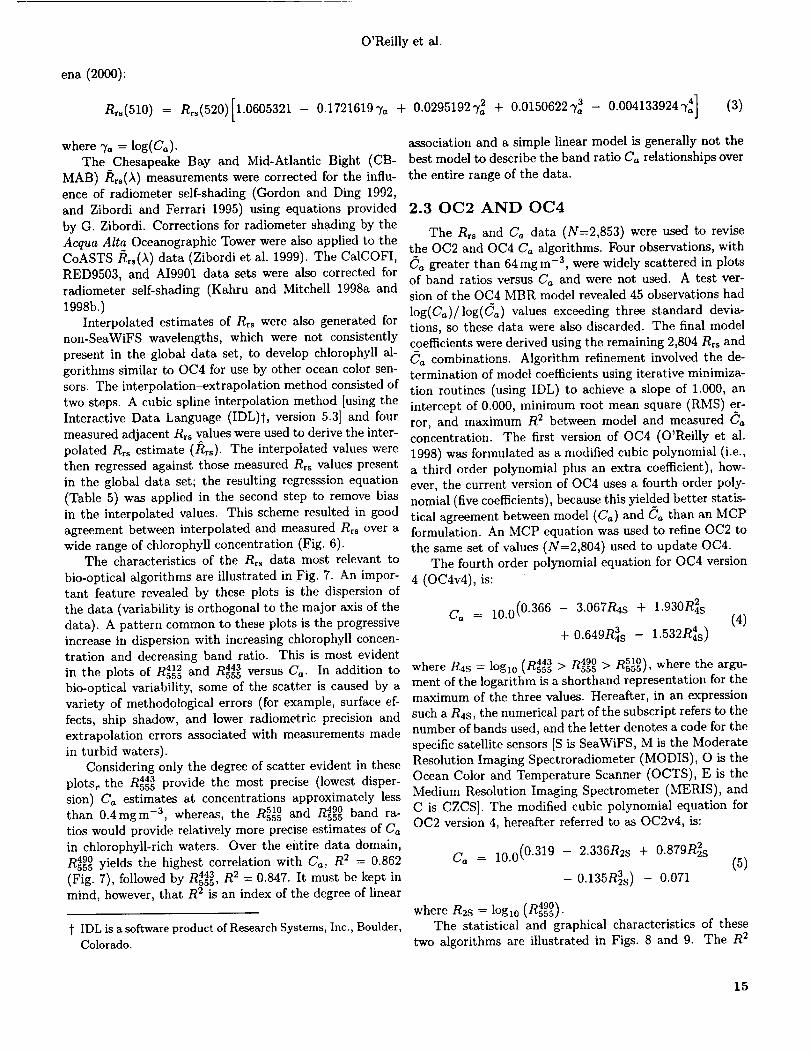
Interpolated estimates of Rrs were also generated for

non-SeaWiFS wavelengths, which were not consistently

present in the global data set, to develop chlorophyll al-

gorithms similar to OC4 for use by other ocean color sen-

sors. The interpolation-extrapolation method consisted of

two steps. A cubic spline interpolation method [using the

Interactive Data Language (IDL)t, version 5.3] and four

measured adjacent R_ values were used to derive the inter-polated R_s estimate (/_rs). The interpolated values were

then regressed against those measured Rr_ values present

in the global data set; the resulting regresssion equation

(Table 5) was applied in the second step to remove bias

in the interpolated values. This scheme resulted in good

agreement between interpolated and measured Rrs over awide range of chlorophyll concentration (Fig. 6).

The characteristics of the Rrs data most relevant to

bio-optical algorithms are illustrated in Fig. 7. An impor-

tant feature revealed by these plots is the dispersion of

the data (variability is orthogonal to the major axis of the

data). A pattern common to these plots is the progressive

increase in dispersion with increasing chlorophyll concen-

tration and decreasing band ratio. This is most evidentin the plots of 19412 and _443• _5_5 "_s55 versus Ca. In addition to

bio-optical variability, some of the scatter is caused by a

variety of methodological errors (for example, surface ef-

fects, ship shadow, and lower radiometric precision andextrapolation errors associated with measurements made

in turbid waters).Considering only the degree of scatter evident in these

plots, the z_443 provide the most precise (lowest disper-"_555

sion) Ca estimates at concentrations approximately less

than 0.4mgm -3, whereas, the _51o and 1949o band ra-"_555 "_555

tios would provide relatively more precise estimates of Ca

in chlorophyll-rich waters. Over the entire data domain,

R490 yields the highest correlation with Ca, R 2 = 0.86255s(Fig. 7), followed by 19443 R 2 = 0.847. It must be kept in_555,

mind, however, that R 2 is an index of the degree of linear

t IDL is a software product of Research Systems, Inc., Boulder,Colorado.

association and a simple linear model is generally not the

best model to describe the band ratio Ca relationships over

the entire range of the data.

2.3 OC2 AND OC4

The Rrs and Ca data (N=2,853) were used to revise

the OC2 and OC4 Ca algorithms. Four observations, withCa greater than 64 mg m -z, were widely scattered in plots

of band ratios versus Ca and were not used. A test ver-sion of the OC4 MBR model revealed 45 observations had

log(Ca)/log(Ca) values exceeding three standard devia-tions, so these data were also discarded. The final model

coefficients were derived using the remaining 2,804 R_s and(_a combinations. Algorithm refinement involved the de-

termination of model coefficients using iterative minimiza-tion routines (using IDL) to achieve a slope of 1.000, an

intercept of 0.000, minimum root mean square (RMS) er-ror, and maximum R 2 between model and measured Ca

concentration. The first version of OC4 (O'Reilly et al.

1998) was formulated as a modified cubic polynomial (i.e.,

a third order polynomial plus an extra coefficient), how-ever, the current version of 0C4 uses a fourth order poly-

nomial (five coefficients), because this yielded better statis-tical agreement between model (Ca) and Ca than an MCP

formulation. An MCP equation was used to refine OC2 to

the same set of values (N=2,804) used to update OC4.

The fourth order polynomial equation for OC4 version

4 (OC4v4), is:

Ca = 10.0 (0.366 - 3.067R4s +

+ 0.649R3s -

1.930R]s

1.532R_s)(4)

[D443 19490 D510_ where the argu-where R4s = lOgl0 _,_555 > -_555 > ,_5551,ment of the logarithm is a shorthand representation for themaximum of the three values. Hereafter, in an expression

such a R4s, the numerical part of the subscript refers to the

number of bands used, and the letter denotes a code for the

specific satellite sensors IS is SeaWiFS, M is the Moderate

Resolution Imaging Spectroradiometer (MODIS), O is theOcean Color and Temperature Scanner (OCTS), E is the

Medium Resolution Imaging Spectrometer (MERIS), and

C is CZCS]. The modified cubic polynomial equation forOC2 version 4, hereafter referred to as OC2v4, is:

Ca = 10.0 (0"319 - 2.336R2s + 0.879R2_s

- 0.135R3s) - 0.071(5)

t'D490_where R2s = logm V _555]-

The statistical and graphical characteristics of thesetwo algorithms are illustrated in Figs. 8 and 9. The R 2

15

16

SeaWiFSPostlaunchCalibration and Validation Analyses, Part 3

1.20

1.10

1.00

0.90

0.80

0.01

+

10.00 IO0.O00.10 1.00

Ca(mg m "a)

1 20! r _l' C)

1.00_ '"0.00 '_

0,80

0.01 0.10 1,00 10.00 100.00

Ca (rag m_

1,20

1.10

1.00

0.90

0.80

0.01

+

0.10

12o 1" i+ _ +_ b+ _-1.10 +

0.80| N=350 t

0.01 0.10 1.00 10.00 100.00

Ca (mg m3)

i;, tN\258 j

0.01 0,10 1.00 10.00 100.00

Ca(mg m_)

1.20j .11o_ _. 'q

°:;I,,.,o,. U1.00 10.00 100.00

Ca (rag m_)

1.201 +

Q_ 1.101" _, -,l=k,'_,...4z-

.... i+ _,_F,_EBIr_ -,-''0C 0.90_ ' .... "

0.80iN=350 . , .

0.01 0.10 1.00 10.00

Ca (rag m"s)

0.01 0.10 1.00

Ca (rag m "_)

°1t

100.00

10.00 100.00

Fig. 6. The ratio of Rrs based on interpolated Rrs (/_) to measured R_ _(R) versus chlorophyll concen-tration (Ca): a)/_510:Rslo; b)/_520:R520; c)/t531:R531; d)/_550:R550; e) R555:R55s; f)/_5_o:Rs60; and g)/_6_:R_85

E .-.:. :.-- __'" • ":!4._,_1_. _._ 1_..- -.__

°:ii"R 2 0,790

0.1 1.0 10,0R412

555

•,-., lO¢?,E

E 1

0.1

0.01R 2:0.847

1R443

555

10

.-, 10¢?,Eo)E 1

v

0.1

0.01 0.01

1 1

400 R51OR 555 sss

Fig. 7. The relationship between -_sss,°4t;-=_ss,°a43,=5_5,_40°and ,_sssl°51°band ratios and chlorophyll concentrationsless than 64mgm -3 (N 2,849, except for _4_ where N = 2,813).---_ _ _555

O'Remyetal.

100

10

0.1

0.010.01

:/_.2804 " .-" .'.,I-"INT:O.O00 " ." :* _L,,('.""SLOPE: 1.000 ,..'; ._,_,,,,_," , .R z" 0 883 ." _..'PL_[_._ " ".'"

............ ,_ : v _°_. ....R :0.2 1 ",4. " ." ""

..-.;:£_..-

:" / ÷_t/" ....................................

....-:_,. :.,,

..... :-,',', ;: ........ ...............

0.1 1 10 100

Ca (mg m-3)

64

32

0-1.00 -0.75 -0.50 -0.25 O.OO 0.25 0.50

log(Ca ICa )

c)

0.75 1.00

100 i , ,),,), ) . .,,H,_ i i 1,1,,, . . ,i,,

/ .¢o., // ..........................................too,/ .b)...t

0.01 0.1 1 10 100

1,0 ' ' )

'0.8

._ o.6LL

_.o., i0.2

0.00.01

Ca Quantiles (rag m-3)

i :;k ;::,,:.......

'_d)d)] ]111 [ I I I I III _ I I IK_II ] _

0,1 1 10 100

Ca (mg m-3)

IO0

10

E 1o)E

v

t_ 0.1

0.01

-,. . ;. ............ e)

%, ._"

O.OOl0.1 1.0 10.0

4_R5_

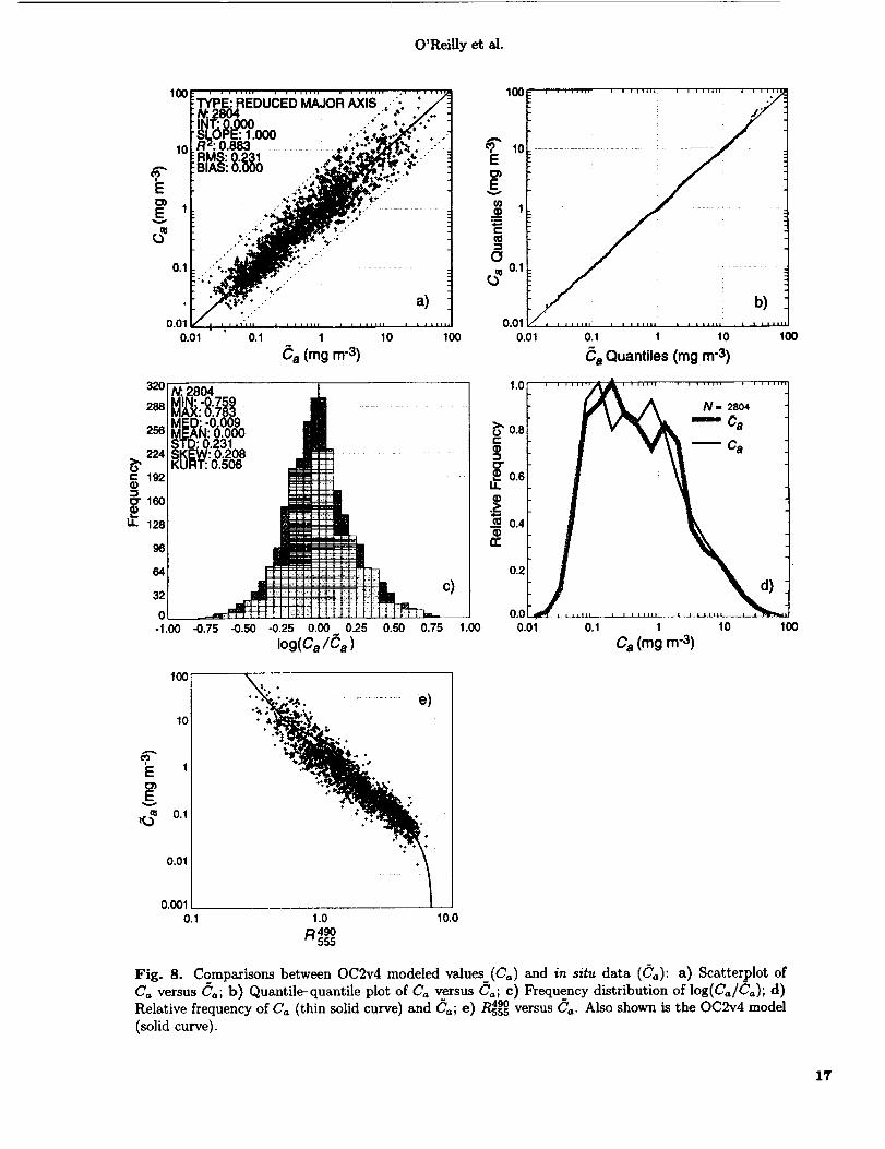
Fig. 8. Comparisons between OC2v4 modeled values (Ca) and in situ data (C=): a) Scatterplot of

Ca versus Ca; b) Quantile-quantile plot of Ca versus Ca; c) Frequency distribution of log(Ca/Ca); d)

Relative frequency of C_ (thin solid curve) and C=; e) Rss549° versus Ca. Also shown is the OC2v4 model

(solid curve).

17

100

10

E

0.1

0.01

18

SeaWiFS Postlaunch Calibration and Validation Analyses, Part 3

0.01 •

INT: 0.000 ': .-_:._Et<.*'"SLOPE: 1.000 . .._._.: .-RZ: 0.892 ,[_.!,_* _._t'_,2" ,-.MS: 0.222 __._:

• "" _, t .+

1 i iiiiii I I I #Ill

0.1 1 10 100

Ca(ragm-3)

340 N: 2804306 MIN:-0.749

MAX: 0.742MED: -0.010

272 MEAN: 0.000STD: 0.222

238 SKEW: 0.295KURT: 0.666

C

_) 170

g138ii

102

68

134

0-1.00 -o.75 -OiSO

100

10

E 1

Ev

1(.3m 0,1

0.01

0.001

-0.25 0.00 0,25 0.50

Iog(Ca/C a )

++

0.75 1.00

0.1 1.0 10.0

R544_ > R49°555>R_5

,,-, 1°° I ........................

OOl / ........ b)o.ol Ol 1 lo lOO

Ca Quantiles (mg m -3)

,o, ........ ,=_^_.......................f\h _ ,=..o. -

o>"0.8 I _%'_'= _ Ca

0.6 iLI.

._ 0.4ID

0.2

O.OL /,, _.,,_..,d_)t d)ii1[ l I I Illl} I I I I LL_L_

0.01 0.1 10 lOO1

Ca (mg m-3)

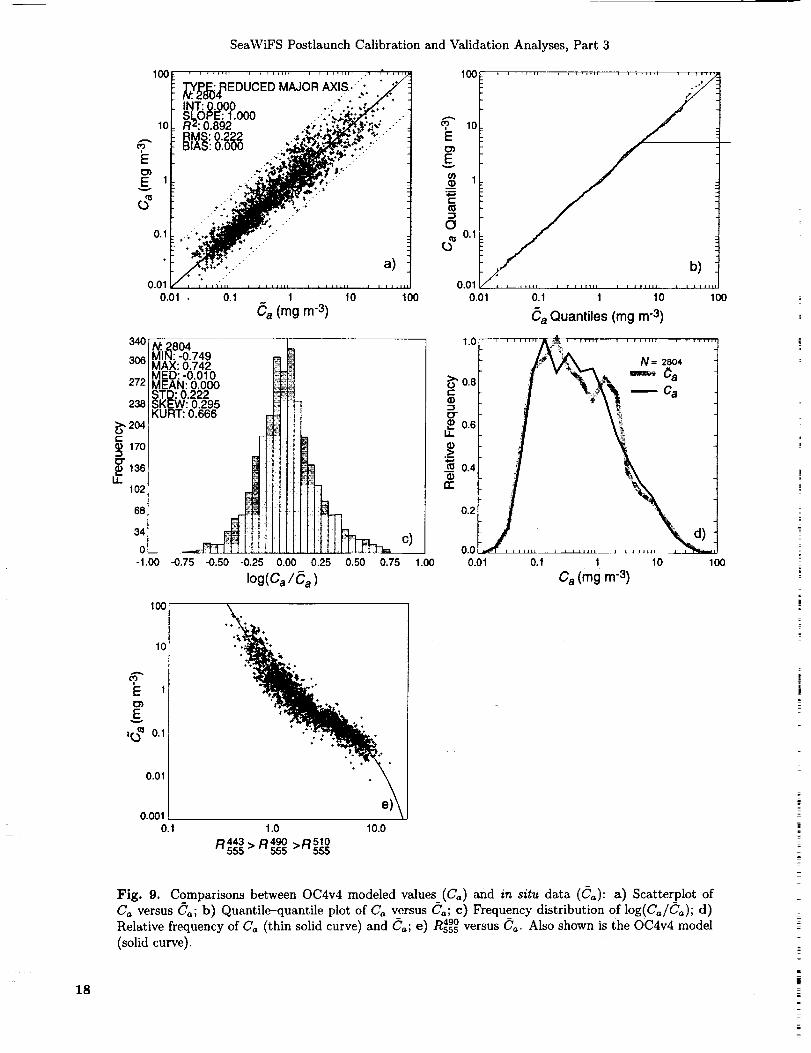
Fig. 9. Comparisons between OC4v4 modeled values (Ca) and in situ data (Ca): a) Scatterplot of

Ca versus Ca; b) Quantile-quantile plot of Ca versus Ca; c) Frequency distribution of log(Ca/Ca); d)

Relative frequency of Ca (thin solid curve) and Ca; e) =_49°=sssversus Ca. Also shown is the OC4v4 model

(solid curve).

O'Reilly et al.

value between Ca and (model) Ca is slightly higher with

OC4 (0.892) than OC2 (0.883). Both models yield a rela-

tive frequency distribution that is approximately congru-ent with the Ca distribution. The OC2 and OC4 models

are extrapolated to a Ca value of 0.001, well below the

lowest concentration (0.008 mgm -_) present in the in situ

data (Figs. 8e and 9e). If clear (clearest) water is oper-ationally defined as Ca = 0.001mgm -3, then the clear

water reflectance ratio /_443_ predicted by OC4 is withink _ _555 )

the theoretical range given in Table 6, whereas the extrap-

olated clear water _490 reflectance ratio for OC2 is greater• _555

than the theoretical clear water estimates.

Because the OC2v4 and OC4v4 algorithms were tuned

to the same data set, their Ca estimates should be very

highly correlated and internally consistent, with a slope

of 1 and an intercept of 0. This is illustrated in Fig. 10.

The reduced scatter (orthogonal to the 1:1 line), centered

at about 1 mgm -3, indicates the region where both algo-rithms use the 490 nm band.

Additional noteworthy characteristics of OC4 are illus-

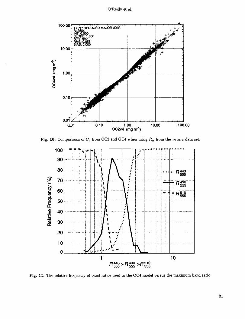
trated in Figs. 11 and 12. The .D443¢555ratio dominates (50%)at MBRs above approximately 2.2, D490 between 2.2 and• _555

1.1, and _510 at MBRs below 1.1 (Fig. 11). With respect to"_555

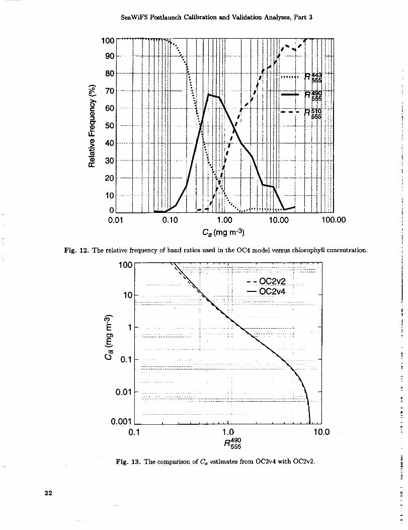
chlorophyll concentration, the ,_443_555ratio dominates (50%)_49o for Cawhen Ca is below approximately 0.33 mg m -3, "_555

between 0.33-1.4 mgm -3, and _51o when Ca exceeds ap-_555

proximately 1.4 mg m -3 (Fig. 12).

Relative to OC2v2, OC2v4 predicts slightly higher Ca

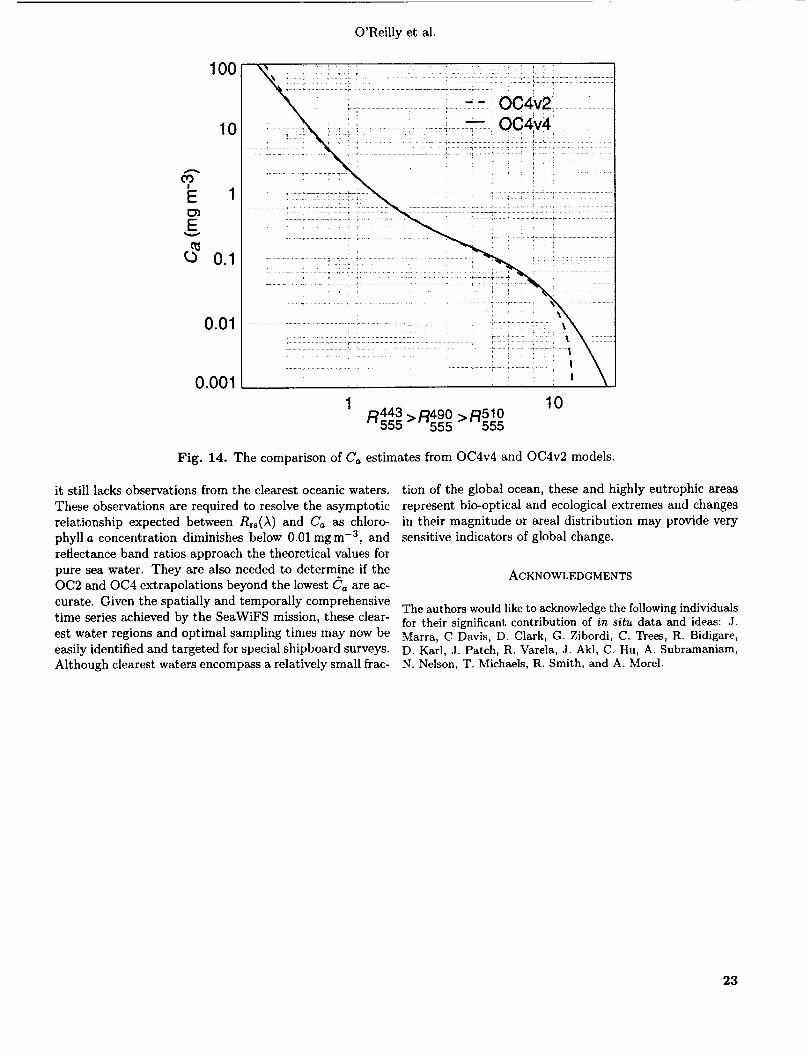
above concentrations of 3 mgm -3 (Fig. 13), while OC4v4

generates slightly lower Ca estimates at very high concen-

trations (Fig. 14). At Ca below 0.03 mg m -a, OC2v4 esti-

mates are very similar to OC2v2, while OC4v4 estimates

are slightly higher than those from OC4v2, particularly so

when Ca is below 0.01 mg m -3. (Version 3 equations were

preliminary and provided to the SeaWiFS Project for test-

ing and evaluation and are not described here.)There is considerable interest and benefit from com-

paring and merging data from various ocean color sensors

(Gregg and Woodward 1998). This is one of the major ob-

jectives of SIMBIOS (McClain and Fargion 1999). In the

particular case of ocean color data merging, one method-

ological issue to be resolved is how data from satellite

sensors having different center band wavelengths can be

merged to generate seamless maps of chlorophyll a distribu-

tion. Among several possible approaches, one is to develop

internally consistent, sensor-specific variations of empirical

chlorophyll a algorithms tuned to the same data set. This

implies a comprehensive suite of in situ measurements at

wavelengths matching the various satellite spectrometers

or perhaps hyperspectral in situ data. To facilitate com-

parisons with SeaWiFS chlorophyll a, MBR algorithms for

several ocean color sensors are presented in Table 7. These

algorithms must be considered as an approximation, be-cause the in situ data set is biased to SeaWiFS channels

and a number of radiometric adjustments were made to

the Rrs(A) data to compensate for wavelength differences

among the sensors (Table 4).

2.4 CONCLUSIONS

A large data set of/_rs and (_a measurements was com-

piled and used to update the OC2 and OC4 bio-optical

chlorophyll a algorithms. The present data set, which is

substantially larger (N=2,853) than that used to develop

the version 2 algorithms (N=1,174), includes samples from

a greater variety of bio-optical provinces, and better rep-

resents oligotrophic and eutrophic waters.

Over the four-decade range in chlorophyll a concentra-

tion encompassed in the data set (0.008-90 mg m-3), the

R490 band ratio is the best overall single band ratio index of555

chlorophyll a concentration. In oligotrophic waters, how-ever, the _443 ratio yields the best correlation with Ca and_555

lowest RMS error, while in waters with chlorophyll concen-

trations exceeding approximately 3 mg m -3, the ps10 ratio"_555

is the best-correlated index. OC4 takes advantage of this

band-related shift in precision, and the well-known shift

of the maximum of Rrs(A) spectra towards higher wave-

lengths with increasing Ca. Dispersion between the OC2model and Ca tended to increase with increasing chloro-

phyll concentrations above 1 mgm -3, whereas dispersion

using OC4 remained relatively low and uniform through-out the range of in situ data. Consequently, OC4 yields a

slightly higher R 2 and lower RMS error than OC2.

Statistical comparisons of algorithm performance with

respect to in situ data, however, provide only partial infor-

mation about their performance when applied to satellite-

derived water-leaving radiances. Operationally, OC4 would

be expected to generate more accurate Ca estimates than

OC2 for several reasons. In oligotrophic water, OC4 would

be expected to provide more accurate Ca estimates than

OC2, because the signal-to-noise ratio (SNR) is greaterin the 443 nm band than the 490 nm band. In eutrophic

waters, strong absorption in the blue region of the spec-trum results in lower SNR for water-leaving radiances re-trieved in the 412nm and 443nm bands relative to the

490rim and 510nm bands. Furthermore, the influence

of the atmospheric correction scheme on the accuracy of

derived water-leaving radiances used in band-ratio algo-rithms must be considered. The SeaWiFS atmospheric cor-

rection algorithm (Gordon and Wang 1994 and Wang 2000)

uses the near infrared bands (765 and 865nm) to char-acterize aerosol optical properties and estimates aerosol

contribution to total radiance in the visible spectrum by

extrapolation. The 510 nm band, being closer to the near

infrared bands, is less prone to extrapolation errors than

the 490 nm and 443 nm bands. In chlorophyll-rich water,

therefore, OC4 would be expected to provide more accu-

rate estimates of Ca than OC2.

The present version of the/_rs(A) and Ca data set rep-

resents a significant improvement in size, quality, and bio-

optical diversity when compared with earlier versions, but

19

SeaWiFSPostlaunchCalibrationandValidationAnalyses,Part3

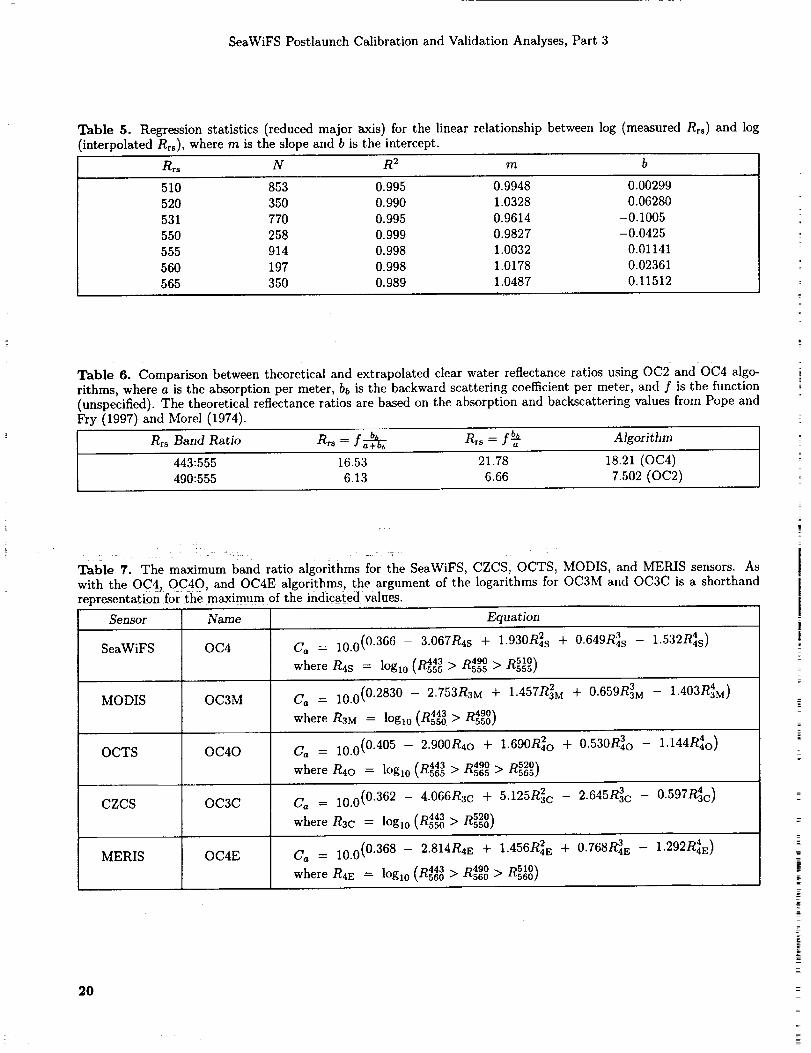
Table 5. Regressionstatistics(reducedmajoraxis)for the linearrelationshipbetweenlog(measuredRrs) and loginterpolated Rrs), where m is the slope and b is the intercept.

Rr8 N R 2 m b

510 853 0.995 0.9948 0.00299

520 350 0.990 1.0328 0.06280

531 770 0.995 0.9614 -0.1005

550 258 0.999 0.9827 -0.0425

555 914 0.998 1.0032 0.01141

560 197 0.998 1.0178 0.02361

565 350 0.989 1.0487 0.11512

Table 6. Comparison between theoretical and extrapolated clear water reflectance ratios using OC2 and OC4 algo-

rithms, where a is the absorption per meter, bb is the backward scattering coefficient per meter, and f is the function(unspecified). The theoretical reflectance ratios are based on the absorption and backscattering values from Pope and

Fry (1997) and Morel (1974).

R,s Band Ratio Rrs = fa+b_bh-- Rr_ = ] _ Algorithm

443:555 16.53 21.78 18.21 (OC4)

490:555 6.13 6.66 7.502 (OC2)

Table 7. The maximum band ratio algorithms for the SeaWiFS, CZCS, OCTS, MODIS, and MERIS sensors. Aswith the OC4, OC40, and OC4E algorithms, the argument of the logarithms for OC3M and OC3C is a shorthand

representation-for-t-he maximum of the indica_e(l values.

Sensor Name Equation

SeaWiFS OC4 Ca -- 10.0 (0.366 - 3.067R4s + 1.930R_s + 0.649R3s - 1.532R_s)

[D443 D490 D510_where R4s = logl0 _,L555 > -_555 > -_5551

MODIS OC3M Ca = 10.0 (0.2830 - 2.753R3M + 1.457R_M + 0.659RIM -- 1.403R_M)

[D443 D490_where R3M ---- lOgl0 V_55o. > "_5501

OCTS OC40 Ca = 10.0 (0.405 - 2.900R4o + 1.690R20 + 0.530R30 - 1-144R4o)

[D443 490 D520_where R4o : log10 _-_565 > R565 > -_5651

CZCS OC3C Ca = 10.0 (0.362 - 4.066R3c + 5.125R2c - 2.645R33c - 0.597R_c)

[D443 ]_520_where R3c : log10 vL550 > -_550!

MERIS OC4E Ca = 10.0 (0.368 - 2.814R4E + 1.456R_E + 0.768R_s - 1.292R_E )[D443 D490 DS10_

where R4E = lOglo _-_56o > ,_560 > -_s60!

2O

O'ReiUyet al.

, 1 , i le,,,

000R: 0.992 +

RMS: 0.058BIAS:0.000 +10.00 +=" .

1.00

0.10 _+.+ + -1.,-I-

0.01

0+01 0.10

• J t llLl , i = ixll J = , i,,

1.00 10.00 100.00

OC2v4 (mg m "3)

Fig. 10. Comparisons of Ca from OC2 and OC4 when using ]_r8 from the in situ data set.

o-e

O

o"

I1)

100

90

80

70

60

50

40

30

20

10

0

, !

_J

i/ i :

1

443 > 490 ,,.._510R555 R555 r.. 555

......i -__ ........i .....................

........_--_:;,, J, _3 ..........!! s55

, : .... R490E 555

! i

i -..,R510i s55

i i

i i......... T'"--, ?:

10

Fig. 11. The relative frequency of band ratios used in the OC4 model versus the maximum band ratio.

21

SeaWiFS Postlaunch Calibrationand ValidationAnalyses,Part 3

22

100 ......._:;=';".

0 ....... {..._._4

0.10

Ca (mg m -3)

LLL

-!.......-4,,J-+_

.....10.00

t_

l]i

, r:

Jii

I':I

1 ]

lil

Ii1,!

4_

100.O0

Fig. 12. The relative frequency of band ratios used in the OC4 model versus chlorophyll concentration.

100

10

E 1

E

rO 0.1

0.01

0.001

0.1

..................................."_ ii -__--__oc2v2:

|...................................................... |

| r I I I i I I I J _ _ _ _ _ _|'

1.0 10.0490

R555

Fig. 13. The comparison of Ca estimates from OC2v4 with OC2v2.

O'Reillyet al.

cO!

E

EV

IO0

I0

1

0.1

0.01

0.001

i...... -_, 0C4v2 ......

i_ ........... ::::, =.0C_v4

: , ] •

...... _"'" "_" " "_"-: _ ""T ................................

1 10R443 >R4_90 >R510

555 555 555

Fig. 14. The comparison of Ca estimates from OC4v4 and OC4v2 models.

it still lacks observations from the clearest oceanic waters.

These observations are required to resolve the asymptotic

relationship expected between Rrs()_) and Ca as chloro-

phyll a concentration diminishes below 0.01 mgm -3, and

reflectance band ratios approach the theoretical values for

pure sea water. They are also needed to determine if theOC2 and OC4 extrapolations beyond the lowest C'_ are ac-

curate. Given the spatially and temporally comprehensive

time series achieved by the SeaWiFS mission, these clear-

est water regions and optimal sampling times may now be

easily identified and targeted for special shipboard surveys.Although clearest waters encompass a relatively small frac-

tion of the global ocean, these and highly eutrophic areas

represent bio-optical and ecological extremes and changesin their magnitude or areal distribution may provide very

sensitive indicators of global change.

ACKNOWLEDGMENTS

The authors would like to acknowledge the following individualsfor their significant contribution of in situ data and ideas: J.Marra, C Davis, D. Clark, G. Zibordi, C. Trees, R. Bidigare,D. Karl, J. Patch, R. Varela, J. Akl, C. Hu, A. Subramaniam,N. Nelson, T. Michaels, R. Smith, and A. Morel.

23

SeaWiFSPostlaunchCalibrationandValidationAnalyses,Part3

Chapter 3

SeaWiFS Algorithm for the Diffuse Attenuation

Coetticient, K(490), Using Water-LeavingRadiances at 490 and 555 nm

JAMES L. MUELLER

CHORS/San Diego State University

San Diego, California

ABSTRACT

A new algorithm has been developed using the ratio of water-leaving radiances at 490 and 555 nm to estimate

K(490), the diffuse attenuation coefficient of seawater at 490 nm. The standard uncertainty of prediction for the

new algorithm is statistically identical to that of the SeaWiFS prelaunch K(490) algorithm, which uses the ratio

of water-leaving radiances at 443 and 490 nm. The new algorithm should be used whenever the uncertainty of

the SeaWiFS determination of water-leaving radiance at 443 is larger than that at 490 nm.

3.1 INTRODUCTION

The attenuation over depth z (in meters), of the spec-

tral downwelling irradiance, Ed(A, z) (in units of mW cm -2nm -1 at wavelength A), is governed by the Beer-LambertLaw:

Ed(A, z) = Ea(A,0-) e -K(_'z)z, (6)

where K(A, z) is the diffuse attenuation coefficient in per

unit meters, averaged over the depth range from just be-

neath the sea surface (z = 0-) to depth z in meters. Gor-

don and McCluney (1975) showed that 90% of the remotelysensed ocean color radiance is reflected from the upper

layer, of depth Z9o, corresponding to the first irradiance

attenuation length, thus satisfying the condition

Ed( ,zgo) = e_l. (7)Ed( )_, O-)

The depth zg0 is found from an irradiance profile, by in-

spection, as the depth where condition (7) is satisfied.

From (6), the remote sensing diffuse attenuation coefficientat wavelength A can be found as K(A) = Zgo1 m -1.

Austin and Petzold (1981) applied simple linear regres-

sion to a sample of spectral irradiance and radiance profiles

to derive a K(490) algorithm of the form

K(490) = Kw(490) + A[L---W-_2)] , (8)

where Kw(490) is the diffuse attenuation coefficient forpure water, Lw()u) and Lw(A2) are "water-leaving radi-

ances at the respective wavelengths of _1 and t2, and

A and B are coefficients derived from linear regression

analysis of the data expressed as In[K(490) - K_(490)]

and ln[Lw(Al)/Lw(A2)]. In Austin and Petzold (1981),Kw(490) = 0.022m -1 was taken from Smith and Baker

(1981), and because the algorithm was derived for CZCS,A1 = 443nm and X2 = 550nm.

The SeaWiFS ocean color instrument has channels at

443 and 555 nm. Mueller and Trees (1997) found a dif-

ferent set of coefficients for (8) using wavelengths )h =443 nm and )_2 - 555 nm, and also used the ratio of nor-

malized water-leaving radiances. The substitution of nor-malized water-leaving radiances in (8) had no significant

effect, but the change in )_2 yielded small, but statisti-cally significant different coefficients A and B. Following

Austin and Petzold (1981), Mueller and Trees (1997) also

assumed K_(490) = 0.022m -1 (Smith and Baker 1981).The Mueller and Trees (1997) result was adopted for the

SeaWiFS prelaunch K(490) algorithm.

SeaWiFS determinations of Lw(443) are persistently

lower than water-leaving radiances that are determinedfrom matched in situ validation measurements. The seri-

ous underestimates of SeaWiFS Lw (443) yield correspond-ingly poor agreement between SeaWiFS and in situ K(490)

determinations. On the other hand, SeaWiFS determina-

tions of Lw(490) and Lw(555) agree much more closelywith validation measurements.

This chapter is the report of an algorithm based on

(8) using 490 and 555nm, which should yield improved

uncertainty in SeaWiFS K(490) estimates. The algorithmalso adopts a reduced value of K_o(490) based on recently

published values of pure water absorption (Pope and Fry

1997).

24

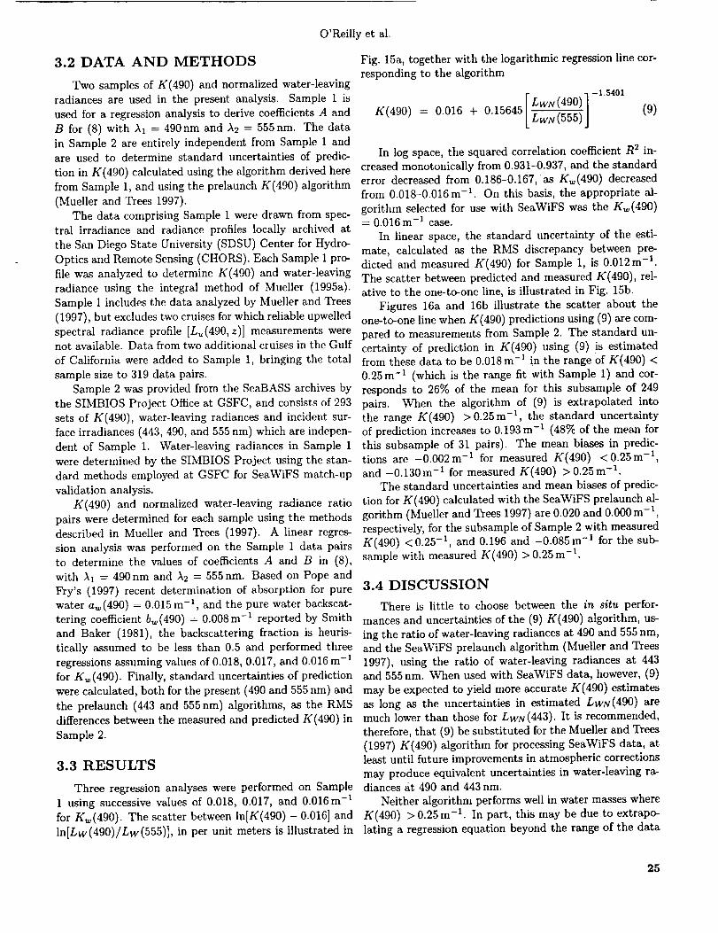
O'Reillyet al.

3.2 DATA AND METHODS

Two samples of K(490) and normalized water-leaving

radiances are used in the present analysis. Sample 1 is

used for a regression analysis to derive coefficients A and

B for (8) with )`1 = 490nm and ),2 = 555nm. The data

in Sample 2 are entirely independent from Sample 1 andare used to determine standard uncertainties of predic-

tion in K(490) calculated using the algorithm derived here

from Sample 1, and using the prelaunch K(490) algorithm

(Mueller and Trees 1997).The data comprising Sample 1 were drawn from spec-

tral irradiance and radiance profiles locally archived at

the San Diego State University (SDSU) Center for Hydro-

Optics and Remote Sensing (CHORS). Each Sample 1 pro-

file was analyzed to determine K(490) and water-leaving

radiance using the integral method of Mueller (1995a).

Sample 1 includes the data analyzed by Mueller and Trees

(1997), but excludes two cruises for which reliable upwelled

spectral radiance profile [L_(490, z)] measurements werenot available. Data from two additional cruises in the Gulf

of California were added to Sample 1, bringing the total

sample size to 319 data pairs.

Sample 2 was provided from the SeaBASS archives by

the SIMBIOS Project Office at GSFC, and consists of 293

sets of K(490), water-leaving radiances and incident sur-

face irradiances (443, 490, and 555 nm) which are indepen-

dent of Sample 1. Water-leaving radiances in Sample 1

were determined by the SIMBIOS Project using the stan-

dard methods employed at GSFC for SeaWiFS match-up

validation analysis.

K(490) and normalized water-leaving radiance ratio

pairs were determined for each sample using the methods

described in Mueller and Trees (1997). A linear regres-

sion analysis was performed on the Sample 1 data pairsto determine the values of coefficients A and B in (8),

with ),1 = 490nm and )`2 = 555nm. Based on Pope and

Fry's (1997) recent determination of absorption for pure

water aw(490) = 0.015 m -1, and the pure water backscat-

tering coefficient bw(490) = 0.008m -1 reported by Smith

and Baker (1981), the backscattering fraction is heuris-

tically assumed to be less than 0.5 and performed three

regressions assuming values of 0.018, 0.017, and 0.016 m -1

for K_ (490). Finally, standard uncertainties of prediction

were calculated, both for the present (490 and 555 nm) and

the prelaunch (443 and 555nm) algorithms, as the RMSdifferences between the measured and predicted K(490) in

Sample 2.

3.3 RESULTS

Three regression analyses were performed on Sample

1 using successive values of 0.018, 0.017, and 0.016m -1

for Kw(490). The scatter between In[K(490) - 0.016] and

ln[Lw(a90)/Lw(555)], in per unit meters is illustrated in

Fig. 15a, together with the logarithmic regression line cor-

responding to the algorithm

r LwN (490) 1 - 1.5401

(49o) = 0.016+ 01 645[ ] (9)

In log space, the squared correlation coefficient R 2 in-

creased monotonically from 0.931-0.937, and the standard

error decreased from 0.186-0.167, as Kw(490) decreasedfrom 0.018-0.(}16m -1. On this basis, the appropriate al-

gorithm selected for use with SeaWiFS was the Kw(490)= 0.016m -l case.

In linear space, the standard uncertainty of the esti-

mate, calculated as the RMS discrepancy between pre-dicted and measured K(490) for Sample 1, is 0.012 m -1.

The scatter between predicted and measured K(490), rel-ative to the one-to-one line, is illustrated in Fig. 15b.

Figures 16a and 16b illustrate the scatter about the

one-to-one line when K(490) predictions using (9) are com-

pared to measurements from Sample 2. The standard un-

certainty of prediction in K(490) using (9) is estimatedfrom these data to be 0.018m -l in the range of K(490) <

0.25m -1 (which is the range fit with Sample 1) and cor-

responds to 26% of the mean for this subsample of 249

pairs. When the algorithm of (9) is extrapolated intothe range K(490) > 0.25 m -1, the standard uncertainty

of prediction increases to 0.193 m -1 (48% of the mean for

this subsample of 31 pairs). The mean biases in predic-tions are -0.002m -1 for measured K(490) <0.25m -1,

and -0.130m -1 for measured K(490) > 0.25m -1.The standard uncertainties and mean biases of predic-

tion for K(490) calculated with the SeaWiFS prelaunch al-

gorithm (Mueller and Trees 1997) are 0.020 and 0.000 m -1,

respectively, for the subsample of Sample 2 with measured

K(490) <0.25 -1, and 0.196 and -0.085m -1 for the sub-sample with measured K(490) > 0.25 m -1.

3.4 DISCUSSION

There is little to choose between the in situ perfor-

mances and uncertainties of the (9) K(490) algorithm, us-

ing the ratio of water-leaving radiances at 490 and 555 nm,and the SeaWiFS prelaunch algorithm (Mueller and Trees

1997), using the ratio of water-leaving radiances at 443and 555 nm. When used with SeaWiFS data, however, (9)

may be expected to yield more accurate K(490) estimatesas long as the uncertainties in estimated LWN(490) are

much lower than those for LWN (443). It is recommended,

therefore, that (9) be substituted for the Mueller and Trees

(1997) K(490) algorithm for processing SeaWiFS data, atleast until future improvements in atmospheric corrections

may produce equivalent uncertainties in water-leaving ra-diances at 490 and 443 nm.

Neither algorithm performs well in water masses where

K(490) >0.25m -1. In part, this may be due to extrapo-lating a regression equation beyond the range of the data

25

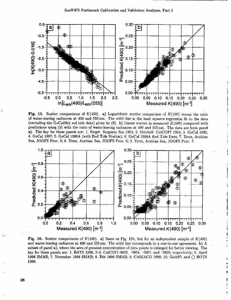
SeaWiFSPostlaunchCalibrationandValidationAnalyses,Part3

26

0"5" a J• _D-0.5 _ ®

_'-1.5-

_'-2.5'

" -3,5,t-.

-4.5-

0.30-

0.25-

!

'_ 0.20-

_" 0.15-

0.10-

Q- 0.05-

-5.5- 0.00-

-0.5 0.0 0.5 1.0 1.5 2.0 2.5 0.00 0.05 0.10 0.15 0.20 0.25 0.30

In[LwN(490)ILwN(555)] Measured K(490) [m -1]

Fig. 15. Scatter comparisons of K(490). a) Logarithmic scatter comparison of K(490) versus the ratio

of water-leaving radiances at 490 and 555 nm. The solid line is the least squares regression fit to the data

(excluding the GoCa198A red tide data) given by (9). b) Linear scatter in measured K(490) compared with

predictions using (9) with the ratio of water-leaving radiances at 490 and 555 nm. The data are from panela). The key for these panels are: 1. Siegel: Sargasso Sea 1994; 2. Mitchell: CalCOFI 1994; 3. GoCal 1995;

4. GoCal 1997; 5. CoCal !998A (with Red Tide Station); 6. GoCal 1998A Red Tide Data; 7. Trees, Arabian

Sea, JGOFS Proc. 2; 8. Trees, Arabian Sea, JGOFS Proc. 6; 9. Trees, Arabian Sea, JGOFS Proc. 7.

1.0- 0.30-

.e.o O.6-o)

"om 0.4-.-_o"o20..- 0.2-

oo iolo

al

®

_®

0.25-

v&...... 0.20-oo')

_" 0.15_® "a8D m

_i(_® "_ 0.10-_5

®_" Q- 0.05.

0.00-

bl

® ®_

_ ®

0.2 0.4 0.6 0.8 i.0 0.oo 0.05 0.10 0.15 020 0.25MeasuredK(490) [m -1] MeasuredK(490) [m "1]

0.30

Fig. 16. Scatter comparisons of K(490). a) Same as Fig. 15b, but for an independent sample of K(490)

and water-leaving radiances at 490 and 555 nm. The solid line corresponds to a one-to-one agreement, b) A

subset of panel a), where the area of greatest concentration of data points is enlarged for better viewing. The

key for these panels are: 1. BATS 1998; 2-5. CalCOFI-9802, -9804, -9807, and -9809, respectively; 6. April

1998 SMAB; 7. November 1998 SMAB; 8. Feb 1999 SMAB; 9. CARIACO 1998; 10. GoA97; and C) HOTS1998.

O'Reillyet al.

usedto fit its coefficients.In thepresentcircumstances,however,it is at leastequallylikelythat the poorpre-dictionsresultfromextremelylargeuncertaintiesin bothK(490) and water-leaving radiances derived from radio-metric measurements near the sea surface in extremely

turbid water masses. In such cases, instrument self shad-

ing, wave focusing, uncertainty in instrument depth de-

termination, and uncertainty in extrapolating L_(£, z) to

the sea surface (especially when the linear slope estima-tion method of analysis is employed) contribute large and

poorly understood uncertainties to measured K(490) and

water-leaving radiances alike. For the near term, the best

policy is to regard SeaWiFS K(490) data with values of

greater than0.25 m -1 with caution and skepticism.

27

SeaWiFSPostlaunchCalibrationandValidationAnalyses,Part3

Chapter 4

Long-Term Calibration History of Several

Marine Environmental Radiometers (MERs)

MARGARET C. O'BRIEN, DAVID W. MENZIES,DAVID A. SIEGEL, AND RAYMOND C. SMITH

ICESS, University of California, Santa Barbara

Santa Barbara, California

ABSTRACT

The accuracy of upper ocean AOPs for the vicarious calibration of ocean color satellites ultimately depends onaccurate and consistent in situ radi0metric data. The SIMBIOS Project is charged with providing estimates

of normalized water-leaving radiance for the SeaWiFS instrument to within 5%. This, in turn, demands that

the radiometric stability of in situ instruments be within 1% with an absolute accuracy of 3%. This chapter

reports on the analysis and reconciliation of the laboratory calibration history for several BSI MERs, models

MER-2040 and -2041, three of which participate in the SeaWiFS Calibration and Validation Program. Thisanalysis includes data using four different FEL calibration lamps, as well as calibrations performed at three

SIRREXs. Barring a few spectral detectors with known deteriorating responses, the radiometers used by UCSB

during the BBOP have been remarkably stable during more than five years of intense data collection. Coefficients

of variation for long-term averages of calibration slopes, for most detectors in the profiling instrument, were less

than 1%. Long-term averages can be applied to most channels, with deviations only after major instrument

upgrades. The methods used here to examine stability accommodate the addition of new calibration data as theybecome available; this enables researchers to closely track any changes in the performance of these instruments

and to adjust the calibration coefficients accordingly. This analysis may serve as a template for radiometer

histories which will be cataloged by the SIMBIOS Project.

4.1 INTRODUCTION

The accuracy of upper ocean AOPs, which are neededfor the vicarious calibration of ocean color satellites, ulti-

mately depends on accurate and consistent in situ radio-metric datal Accurate validation of SeaWiFS demands an

in-water radiometric stability within 1%, with an accuracy

of 3% (Mueller and Austin 1995). Considerable energy

has been spent refining calibration protocols for profiling

radiometers. The SeaWiFS Project Office has sponsored

several workshops through its Calibration and Validation

Program, which have yielded significant improvements in

the research community's ability to provide accurate AOPestimates. These include the SIRREXs, conducted annu-

ally since 1992 (Mueller 1993, Mueller et al. 1994, Mueileret al. 1996, and Johnson et al. 1996), as well as the Data

Analysis Round-Robin (DARR) workshop in 1994 (Siegel

et al. 1995).At the Institute for Computational Earth System Sci-

ence (ICESS) at UCSB, several research projects providevalidation data for ocean color satellites. These include

BBOP in the Sargasso Sea, the Plumes and Blooms Project

28

in the Santa Barbara Channel, and the Palmer Area Long

Term Ecological Research (LTER) site on the AntarcticPeninsula. The ICESS Calibration Laboratory and BBOP -

have participated in all of the workshops held by the Cal-

ibration and Validation Program.

This report presents an analysis of the multiyear lab-oratory calibration history for several BSI MERs, models -MER-2040 and -2041. This analysis includes data using :

four different FEL calibration lamps, as well as calibra- -

tions performed at three SIRREX exercises. This reportwill show that, barring a few sensors with known deteri- ---

orating responses, the radiometers used by UCSB during

BBOP have been remarkably stable during six years ofintense data collection.

4.2 ICESS FACILITY AND METHODS

The ICESS optical calibration facility is housed in aclimate-controlled room. A 1.2 x 1.8 m (4x 6 ft) optical ta-

ble, with threaded holes arranged in a 2.5 cm (1 in) grid,

supports one end of a 2.4 m (8 ft)|ong Optical rail. h black,

wooden baffle with a 25.4cm (10 in) diameter hole strad-

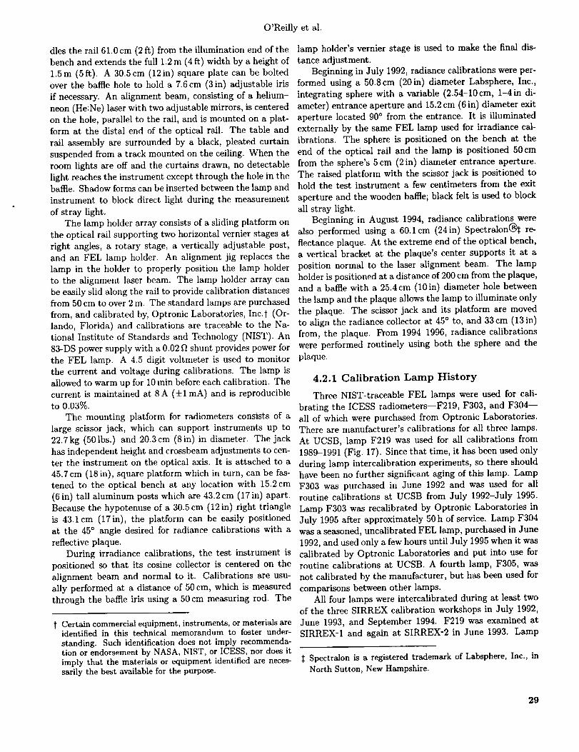
O'Reillyet al.

dlestherail61.0cm(2ft) fromtheilluminationendofthebenchandextendsthefull 1.2m(4ft) widthbyaheightof1.5m (5ft). A 30.5cm(12in) squareplatecanbeboltedoverthebaffleholeto holda 7.6cm(3in) adjustableirisif necessary.An alignmentbeam,consistingof ahelium-neon(He:Ne)laserwithtwoadjustablemirrors,iscenteredonthehole,parallelto therail,andismountedonaplat-format thedistalendof theopticalrail. Thetableandrail assemblyaresurroundedby a black,pleatedcurtainsuspendedfromatrackmountedontheceiling.Whentheroomlightsareoffandthecurtainsdrawn,nodetectablelightreachestheinstrumentexceptthroughtheholein thebaffle.Shadowformscanbeinsertedbetweenthelamp and

instrument to block direct light during the measurement

of stray light.

The lamp holder array consists of a sliding platform on

the optical rail supporting two horizontal vernier stages at

right angles, a rotary stage, a vertically adjustable post,

and an FEL lamp holder. An alignment jig replaces the

lamp in the holder to properly position the lamp holder

to the alignment laser beam. The lamp holder array can

be easily slid along the rail to provide calibration distances

from 50 cm to over 2 m. The standard lamps are purchased

from, and calibrated by, Optronic Laboratories, Inc3 (Or-

lando, Florida) and calibrations are traceable to the Na-

tional Institute of Standards and Technology (NIST). An

83-DS power supply with a 0.02 f_ shunt provides power for

the FEL lamp. A 4.5 digit voltmeter is used to monitor

the current and voltage during calibrations. The lamp is

allowed to warm up for 10 min before each calibration. The

current is maintained at 8A (=i=l mA) and is reproducibleto 0.03%.

The mounting platform for radiometers consists of a

large scissor jack, which can support instruments up to

22.7kg (501bs.) and 20.3cm (8in) in diameter. The jack

has independent height and crossbeam adjustments to cen-

ter the instrument on the optical axis. It is attached to a

45.7 cm (18 in), square platform which in turn, can be fas-tened to the optical bench at any location with 15.2cm

(6 in) tall aluminum posts which are 43.2cm (17 in) apart.

Because the hypotenuse of a 30.5 cm (12 in) right triangle

is 43.1cm (17in), the platform can be easily positionedat the 45 ° angle desired for radiance calibrations with a

reflective plaque.

During irradiance calibrations, the test instrument is

positioned so that its cosine collector is centered on the

alignment beam and normal to it. Calibrations are usu-

ally performed at a distance of 50 cm, which is measured

through the baffle iris using a 50 cm measuring rod. The

[ Certain commercial equipment, instruments, or materials areidentified in this technical memorandum to foster under-standing. Such identification does not imply recommenda-tion or endorsement by NASA, NIST, or ICESS, nor does itimply that the materials or equipment identified are neces-sarily the best available for the purpose.

lamp holder's vernier stage is used to make the final dis-

tance adjustment.

Beginning in July 1992, radiance calibrations were per-

formed using a 50.8cm (20in) diameter Labsphere, Inc.,

integrating sphere with a variable (2.54-10cm, 1-4in di-

ameter) entrance aperture and 15.2 cm (6 in) diameter exitaperture located 90 ° from the entrance. It is illuminated

externally by the same FEL lamp used for irradiance cal-

ibrations. The sphere is positioned on the bench at the

end of the optical rail and the lamp is positioned 50 cm

from the sphere's 5 cm (2 in) diameter entrance aperture.The raised platform with the scissor jack is positioned tohold the test instrument a few centimeters from the exit

aperture and the wooden baffle; black felt is used to block

all stray light.

Beginning in August 1994, radiance calibrations werealso performed using a 60.1cm (24in) Spectralon(_ re-

flectance plaque. At the extreme end of the optical bench,

a vertical bracket at the plaque's center supports it at a

position normal to the laser alignment beam. The lamp

holder is positioned at a distance of 200 cm from the plaque,and a baffle with a 25.4 cm (10 in) diameter hole between

the lamp and the plaque allows the lamp to illuminate only

the plaque. The scissor jack and its platform are moved

to align the radiance collector at 45 ° to, and 33 cm (13 in)

from, the plaque. From 1994-1996, radiance calibrations

were performed routinely using both the sphere and the

plaque.

4.2.1 Calibration Lamp History

Three NIST-traceable FEL lamps were used for cali-

brating the ICESS radiometers--F219, F303, and F304--

all of which were purchased from Optronic Laboratories.

There are manufacturer's calibrations for all three lamps.

At UCSB, lamp F219 was used for all calibrations from

1989-1991 (Fig. 17). Since that time, it has been used only

during lamp intercalibration experiments, so there should

have been no further significant aging of this lamp. Lamp

F303 was purchased in June 1992 and was used for allroutine calibrations at UCSB from July 1992-July 1995.

Lamp F303 was recalibrated by Optronic Laboratories in

July 1995 after approximately 50 h of service. Lamp F304

was a seasoned, uncalibrated FEL lamp, purchased in June

1992, and used only a few hours until July 1995 when it was

calibrated by Optronic Laboratories and put into use for

routine calibrations at UCSB. A fourth lamp, F305, was

not calibrated by the manufacturer, but has been used for

comparisons between other lamps.

All four lamps were intercalibrated during at least two

of the three SIRREX calibration workshops in July 1992,

June 1993, and September 1994. F219 was examined at

SIRREX-1 and again at SIRREX-2 in June 1993. Lamp

:_ Spectralon is a registered trademark of Labsphere, Inc., in

North Sutton, New Hampshire.

29

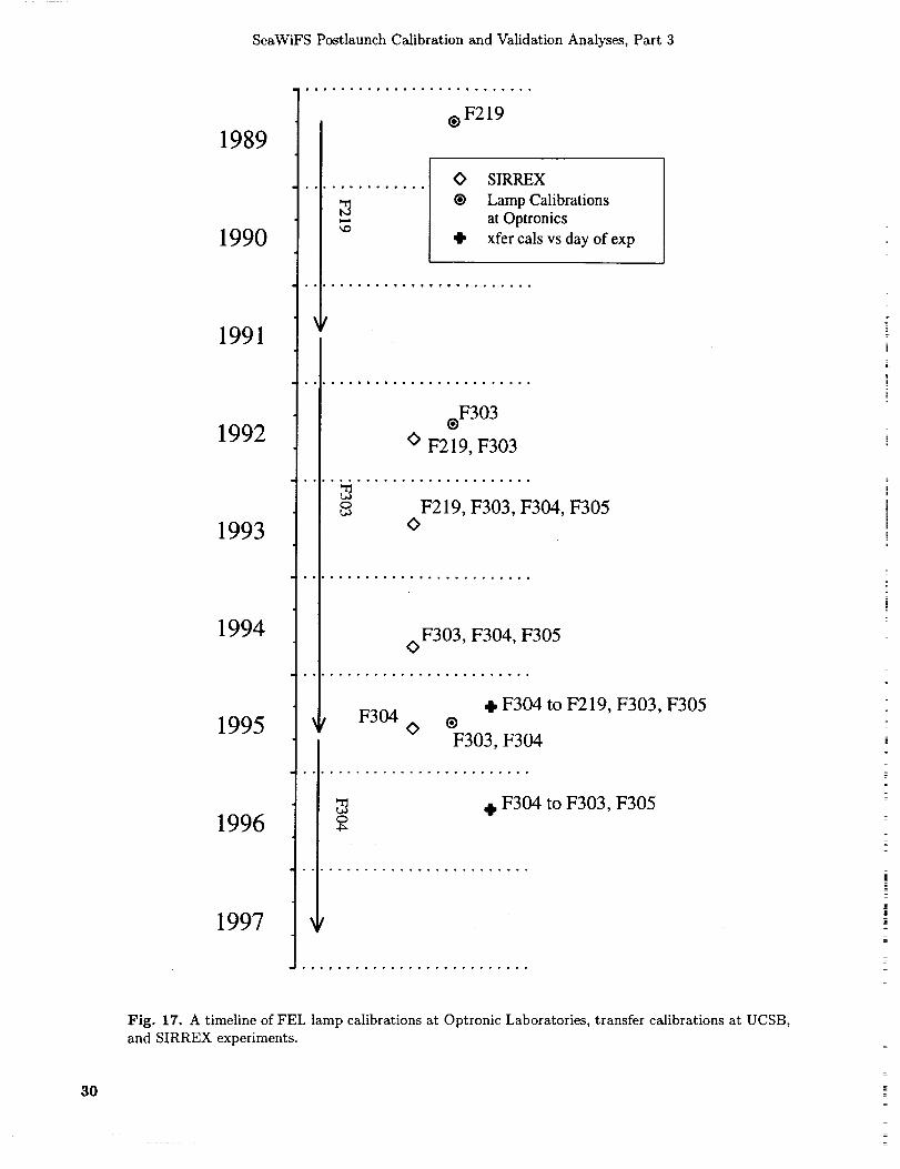
SeaWiFSPostlaunchCalibrationandValidationAnalyses,Part3

1989

1990

1991

1992

1993

1994

1995

1996

1997

,°°°°.°°.°°°° ..... ,..,°.,°

®F219

°,.°°°°°°,°0 SIRREX

® Lamp Calibrations

at Optronics

41, xfer cals vs day of exp

®F303

O F219, F303

....... ° ............ ° ° ,

_ F219, F303, F304, F305O

oF303, F304, F305

F304O

,I, F304 to F219, F303, F305®

F303, F304

F304to F303, F305

30

Fig. 17. A timeline of FEL lamp calibrations at Optronic Laboratories, transfer calibrations at UCSB,

and SIRREX experiments.

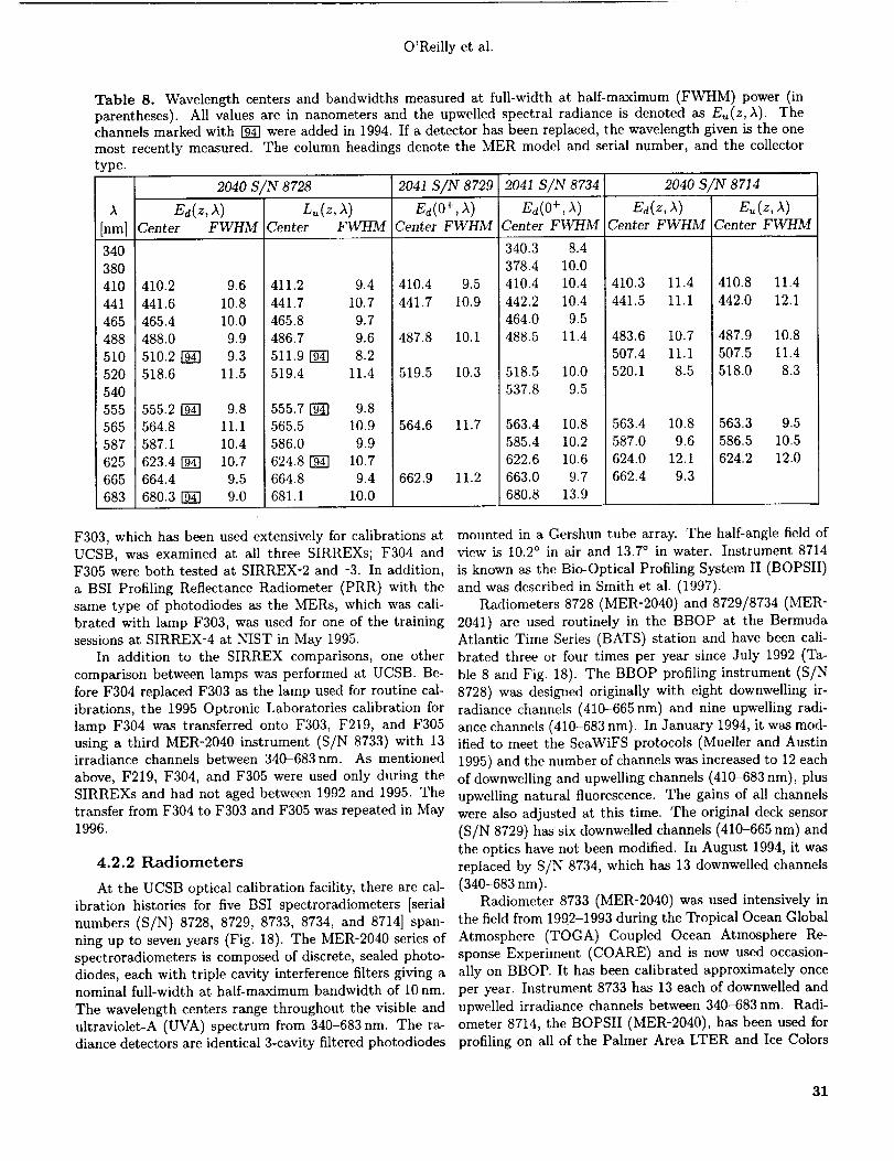
O'Reillyet al.

Table 8. Wavelengthcentersandbandwidthsmeasuredat full-widthat half-maximum(FWHM)power(inparentheses).All valuesarein nanometersandtheupwelledspectralradianceis denotedasE_,(z,£). Thechannels marked with [_ were added in 1994. If a detector has been replaced, the wavelength given is the one

most recently measured. The column headings denote the MER model and serial number, and the collector

type.

2040 S/N

[nm] Center FWHM

340

380410 410.2 9.6

441 441.6 10.8

465 465.4 10.0

488 488.0 9.9

510 510.2 [-_ 9.3

520 518.6 11.5

540

555 555.2 I-_ 9.8

565 564.8 11.1

587 587.1 10.4

625 623.4 [_] 10.7

665 664.4 9.5

683 680.3 [_ 9.0

8728

Center FWHM

411.2 9.4

441.7 10.7

465.8 9.7

486.7 9.6

511.9 I-_ 8.2519.4 11.4

555.7 _ 9.8565.5 10.9

586.0 9.9

624.8 [_J 10.7664.8 9.4

681.1 10.0

2041 S/N 8729

Ed(O+,Center FWHM

410.4 9.5

441.7 10.9

487.8 10.1

519.5 10.3

564.6

662.9

11.7

11.2

2041 SIN 8734

Ed(0+, X)Center FWHM

340.3 8.4

378.4 10.0

410.4 10.4

442.2 10.4

464.0 9.5

488.5 11.4

2040 S/N 8714

Center FWHM Center FWHM

410.3 11.4 410.8 11.4

441.5 11.1 442.0 12.1

483.6 10.7 487.9 10.8

507.4 11.1 507.5 11.4

520.1 8.5 518.0 8.3

563.3 9.5

586.5 10.5

624.2 12.0

563.4 10.8

587.0 9.6

624.0 12.1

662.4 9.3

518.5 10.0

537.8 9.5

563.4 10.8

585.4 10.2

622.6 10.6

663.0 9.7

680.8 13.9

F303, which has been used extensively for calibrations atUCSB, was examined at all three SIRREXs; F304 andF305 were both tested at SIRREX-2 and -3. In addition,

a BSI Profiling Reflectance Radiometer (PRR) with the

same type of photodiodes as the MERs, which was cali-brated with lamp F303, was used for one of the trainingsessions at SIRREX-4 at NIST in May 1995.

In addition to the SIRREX comparisons, one other

comparison between lamps was performed at UCSB. Be-

fore F304 replaced F303 as the lamp used for routine cal-ibrations, the 1995 Optronic Laboratories calibration for

lamp F304 was transferred onto F303, F219, and F305

using a third MER-2040 instrument (S/N 8733) with 13irradiance channels between 340-683nm. As mentioned

above, F219, F304, and F305 were used only during the

SIRREXs and had not aged between 1992 and 1995. Thetransfer from F304 to F303 and F305 was repeated in May

1996.

4.2.2 Radiometers

At the UCSB optical calibration facility, there are cal-

ibration histories for five BSI spectroradiometers [serial

numbers (S/N) 8728, 8729, 8733, 8734, and 8714] span-

ning up to seven years (Fig. 18). The MER-2040 series ofspectroradiometers is composed of discrete, sealed photo-

diodes, each with triple cavity interference filters giving anominal full-width at halbmaximum bandwidth of 10 nm.

The wavelength centers range throughout the visible andultraviolet-A (UVA) spectrum from 340-683 nm. The ra-diance detectors are identical 3-cavity filtered photodiodes

mounted in a Gershun tube array. The half-angle field of

view is 10.2 ° in air and 13.7 ° in water. Instrument 8714

is known as the Bio-Optical Profiling System II (BOPSII)

and was described in Smith et al. (1997).

Radiometers 8728 (MER-2040) and 8729/8734 (MER-

2041) are used routinely in the BBOP at the BermudaAtlantic Time Series (BATS) station and have been cali-

brated three or four times per year since July 1992 (Ta-

ble 8 and Fig. i8). The BBOP profiling instrument (S/N

8728) was designed originally with eight downwelling ir-

radiance channels (410-665 nm) and nine upwelling radi-

ance channels (410-683 nm). In January 1994, it was mod-ified to meet the SeaWiFS protocols (Mueller and Austin

1995) and the number of channels was increased to 12 eachof downwelling and upwelling channels (410-683 nm), plus

upwelling natural fluorescence. The gains of all channels

were also adjusted at this time. The original deck sensor

(S/N 8729) has six downwelled channels (410-665 nm) and

the optics have not been modified. In August 1994, it was

replaced by S/N 8734, which has 13 downwelled channels

(340-683 nm).Radiometer 8733 (MER-2040) was used intensively in

the field from 199.2-1993 during the Tropical Ocean Global

Atmosphere (TOGA) Coupled Ocean Atmosphere Re-

sponse Experiment (COARE) and is now used occasion-

ally on BBOP. It has been calibrated approximately once

per year. Instrument 8733 has 13 each of downwelled and

upwelled irradiance channels between 340-683 nm. Radi-ometer 8714, the BOPSII (MER-2040), has been used for

profiling on all of the Palmer Area LTER and Ice Colors

31

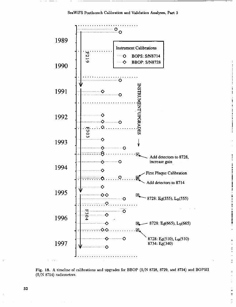
SeaWiFS Postlaunch Calibration and Validation Analyses, Part 3

1989

1990

1991

1992

1993

1994

1995

1996

1997

i ol,,,ololt g._lo.,o.o..,o,

...............................................

...............................................

. "fi .......... I_tmment Calibrations

I ......O BOPS: S/N8714

_OP: S/N8728

o o _

• i° ,.°°°°°o°°o,°°°o..°°°_

° __ .................0 _

O

° i0

............. _ Add detectors to 8728,

0 .................0 increase gain

O

First Plaque Calibration

Add detectors to 8714O

....t_ ....................<> oi 4_

....! .............................O _ 8728: Ed(665), Lu(665)

i, oo............%,t .............................O ..................O 8728: Ed(510), Lu(510)

+ O 8734: Ed(340)

Fig. 18. A timeline of calibrations and upgrades for BBOP (S/N 8728, 8729, and 8734) and BOPSII

(S/N 8714) radiometers.

32

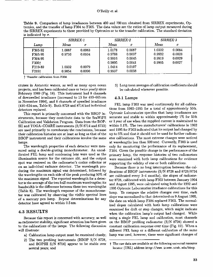
O'Reilly et al.

Table 9. Comparison of lamp irradiances between 400 and 700 nm obtained from SIRREX experiments, Op-tronics, and the transfer of lamp F304 to F305. The data values are the ratios of lamp output measured duringthe SIRREX experiments to those provided by Optronics or to the transfer calibration. The standard deviationis indicated by a.

SIRREX- 1 SIRREX- 2 SIRREX- 3

Lamp Mean a Mean (7 Mean a

F303-92

F303-95

F304-95

F305tF219-89

F219t

1.0087 0.0083

0.9710 0.0104

1.0332 0.0079

0.9854 0.0096

1.0178 0.00870.9788 0.0037

0.9916 0.0045

0.9895 0.0041

1.0414 0.0107

0.9937 0.0038

1.0332 0.0084

0.9932 0.0028

0.9919 0.0029

0.9905 0.0027

t Transfer calibration from F304.

cruises in Antarctic waters, as well as many open ocean

projects, and has been calibrated once or twice yearly since

February 1989 (Fig. 18). This instrument had 8 channels

of downwelled irradiance (increased to 13 for 410-665 nmin November 1994), and 8 channels of upwelled irradiance

(410-624 nm, Table 9). Both 8728 and 8714 had individualdetectors replaced.

This report is primarily concerned with the BBOP in-struments, because they contribute data to the SeaWiFS

Calibration and Validation Program. Data from the BOP-

SII and TOGA-COARE instruments (S/N 8714 and 8733)are used primarily to corroborate the conclusions, because

their calibration histories are at least as long as that of theBBOP instrument and their calibrations involve the same

lamps.The wavelength properties of each detector were mea-

sured using a double-grating monochrometer. An uncal-

ibrated FEL lamp and condensing lens were used as theillumination source for the entrance slit, and the output

spot was centered on the radiometer's cosine collector or

on an individual radiance detector. The wavelength pro-

ducing the maximum signal was determined, followed bythe wavelengths on each side of the peak producing 50% ofthe maximum signal. The reported wavelength for a detec-

tor is the average of the two half-maximum wavelengths; itsbandwidth is the difference between these two wavelengths

(Table 8). The wavelength response of the monochrome-ter was calibrated by observing the visible spectral lines

of a mercury pen lamp. Repeat determinations for any

detector have agreed to within 0.5 nm.

4.3 RESULTS

Because this report is concerned with accuracy, as well

as radiometer stability, significant attention has been given

to the calibrations of the lamps. The following discussionwill illustrate:

a) Calibration lamp output must be examined closely;

2) The two profiling instruments (BBOP S/N 8728,and BOPSII S/N 8714) appear to be stable over

several years; and

3) Long-term averages of calibration coefficients shouldbe calculated whenever possible.

4.3.1 Lamps

FEL lamp F303 was used continuously for all calibra-

tions from 1992-1995 for a total of approximately 50 h.

Optronic Laboratories specifies that lamp irradiances areaccurate and stable to within approximately 1% for 50h

or 1 year of use when the supplied current is maintained towithin 0.1%. The two manufacturers' calibrations in 1992

and 1995 for F303 indicated that its output had changed by

up to 5% and that it should not be used for further radiom-

eter calibrations. The most extreme changes were noticed

at wavelengths less than 500 nmt. Currently, F303 is used

only for monitoring the performance of its replacement,

F304. Given the possible change in the performance of the

primary lamp, the response histories o_[ two radiometers

were examined with both lamp calibrations for evidence

supporting the validity of one or both calibrations.

Because there is no long interruption between the cal-

ibrations of BBOP instruments (S/N 8728 and 8729/8734

are calibrated every 3-4 months), the slopes of radiome-

ter 8728, calibrated with lamp F303 between January 1994

and August 1995, were calculated using both the 1992 and

1995 Optronic Laboratories irradiance calibrations for this

lamp. To compare the relative changes over time, each

slope was normalized to that determined on 9 August 1995,the date on which lamp F304 replaced F303. The normal-

ized slopes calculated with both lamp calibrations were

examined for drift or step changes, which might indicate

when the calibration lamp's output had changed. While

using a single FEL lamp and calibration, most channels

on the BBOP profiling radiometer (S/N 8728) showed a

constant calibration response over time (Fig. 19). When a

different FEL lamp or a different calibration of the same

lamp was used, however, there were significant changes of

t The raw data are available at the following universal resource

locator (URL) address http://w_n_, icess, ucsb. edu/bbop.

33

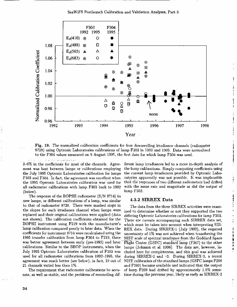
SeaWiFSPostlaunchCalibrationandValidationAnalyses,Part3

1.08

o._,,4o 1.06

o(.9 1.04

._ 1.02

i 1.000.98

F303 F3041992 1995 1995

Ea(410) @ O •

Ed(488) IZl [] •

Ed(565) • ix •

Ea(683) ® 0 • ®

®

• []® [] •®

_) • ®

® ® o

norm

I , i I i i I , i l i

1994 1995 1996 1997

0Z 0.96 ' ' J ' '

1992 1993 1998

Year

Fig. 19. The normalized calibration coefficients for four downwelling irradiance channels (radiometer

8728) using Optronic Laboratories calibrations of lamp F303 in 1992 and 1995. Data were normalized

to the F304 values measured on 9 August 1995, the first date for which lamp F304 was used

2-6% in the coefficients for most of the channels. Agree-

ment was best between lamps or calibrations employing

the July 1995 Optronic Laboratories calibration for lamps

F303 and F304. In fact, the agreement was excellent whenthe 1995 Optronic Laboratories calibration was used for

all radiometer calibrations with lamp F303 back to 1992

(below).

The response of the BOPSII radiometer (S/N 8714) to

new lamps, or different calibrations of a lamp, was similarto that of radiometer 8728. There were marked steps in

the slopes for each irradiance channel when lamps were

replaced and their original calibrations were applied (datanot shown). The calibration coefficients obtained for the

BOPSII instrument using F219 with the manufacturer's

lamp calibration compared poorly to later data. When the

coefficients for instrument 8714 were recalculated using the1995 transfer calibration from lamp F304 to F219, there

ferent lamp irradiances led to a more in-depth analysis of

the lamp calibrations. Simply computing coefficients usingthe current lamp irradiances provided by Optronic Labo-

ratories apparently was not possible. It was implausiblethat the responses of two different radiometers had drifted

with the same rate and magnitude as did the output oflamp F303.

4.3.2 SIRREX Data

The data from the three SIRREX activities were exam-

ined to determine whether or not they supported the two

differing Optronic Laboratories calibrations for lamp F303.

There are caveats accompanying each SIRREX data set,which must be taken into account when interpreting SIR-

REX data. During SIRREX-1 (July 1992), the requireduncertainty of 1% was not achieved when transferring the

NIST scale of spectral irradiance from the Goddard Space

was better agreement between early (pre-1992) and later '-Flight _center (GSFC) stan_arcl:iamp (F267) to the othercalibrations. Similar to the BBOP instruments, when the lamps (Johnson et al. 1996). The data are, however, in-

July 1995 Optronic Laboratories calibration of F303 was cluded here for completeness, and this goal was achieved

used for all radiometer calibrations from 1992-1995, the during SIRREX-2 and -3. During SIRREX-3, a recent

agreement was much better (see below); in fact, 19 out of NIST calibration of the standard lamps (GSFC lamps F26821 channels varied less than 1%. and F269) became available and indicated that the output

The requirement that radiometer calibrations be accu- of lamp F269 had drifted by approximately 1.5% some-

rate, as well as stable, and the problems of reconciling dif- time during the previous year, likely as early as SIRREX-2

34

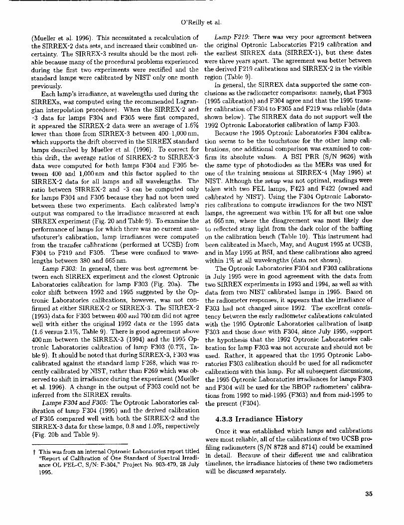
O'Reillyet al.

(Muelleret al.1996).Thisnecessitateda recalculationoftheSIRREX-2datasets,andincreasedtheircombinedun-certainty.TheSIRREX-3resultsshouldbethemostreli-ablebecausemanyoftheproceduralproblemsexperiencedduringthe first two experimentswererectifiedandthestandardlampswerecalibratedby NISTonlyonemonthpreviously.

Eachlamp'sirradiance,atwavelengthsusedduringtheSIRREXs,wascomputedusingtherecommendedLagran-gianinterpolationproceduret.WhentheSIRREX-2and-3 datafor lampsF304andF305werefirst compared,it appearedtheSIRREX-2datawereanaverageof 1.6%lowerthanthosefromSIRREX-3between400-1,000nm,whichsupportsthedriftobservedin theSIRREXstandardlampsdescribedby Muelleret al. (1996).Tocorrectforthisdrift, theaverageratiosof SIRREX-2to SIRREX-3datawerecomputedfor bothlampsF304andF305be-tween400 and 1,000nm and this factor applied to the

SIRREX-2 data for all lamps and all wavelengths. The

ratio between SIRREX-2 and -3 can be computed only

for lamps F304 and F305 because they had not been used

between these two experiments. Each calibrated lamp's

output was compared to the irradiance measured at each

SIRREX experiment (Fig. 20 and Table 9). To examine the

performance of lamps for which there was no current man-

ufacturer's calibration, lamp irradiances were computed

from the transfer calibrations (performed at UCSB) fromF304 to F219 and F305. These were confined to wave-

lengths between 380 and 665 nm.

Lamp F303: In general, there was best agreement be-tween each SIRREX experiment and the closest Optronic

Laboratories calibration for lamp F303 (Fig. 20a). The

color shift between 1992 and 1995 suggested by the Op-

tronic Laboratories calibrations, however, was not con-firmed at either SIRREX-2 or SIRREX-3. The SIRREX-2

(1993) data for F303 between 400 and 700 nm did not agreewell with either the original 1992 data or the 1995 data

(1.6 versus 2.1%, Table 9). There is good agreement above

400nm between the SIRREX-3 (1994) and the 1995 Op-tronic Laboratories calibration of lamp F303 (0.7%, Ta-

ble 9). It should be noted that during SIRREX-3, F303 was

calibrated against the standard lamp F268, which was re-

cently calibrated by NIST, rather than F269 which was ob-served to shift in irradiance during the experiment (Mueller

et al. 1996). A change in the output of F303 could not beinferred from the SIRREX results.

Lamps F304 and F305: The Optronic Laboratories cal-

ibration of lamp F304 (1995) and the derived calibration

of F305 compared well with both the SIRREX-2 and the

SIRREX-3 data for these lamps, 0.8 and 1.0%, respectively

(Fig. 20b and Table 9).

t This was from an internal Optronic Laboratories report titled"Report of Calibration of One Standard of Spectral Irradi-ance OL FEL-C, S/N: F-304," Project No. 903-479, 28 July1995.

Lamp F219: There was very poor agreement between

the original Optronic Laboratories F219 calibration and

the earliest SIRREX data (SIRREX-1), but these dates

were three years apart. The agreement was better betweenthe derived F219 calibrations and SIRREX-2 in the visible

region (Table 9).

In general, the SIRREX data supported the same con-clusions as the radiometer comparisons: namely, that F303

(1995 calibration ) and F304 agree and that the 1995 trans-fer calibration of F304 to F305 and F219 was reliable (data

shown below). The SIRREX data do not support well the

1992 Optronic Laboratories calibration of lamp F303.

Because the 1995 Optronic Laboratories F304 calibra-

tion seems to be the touchstone for the other lamp cali-

brations, one additional comparison was examined to con-

firm its absolute values. A BSI PRR (S/N 9626) with

the same type of photodiodes as the MERs was used for

one of the training sessions at SIRREX-4 (May 1995) at

NIST. Although the setup was not optimal, readings were

taken with two FEL lamps, F423 and F422 (owned and

calibrated by NIST). Using the F304 Optronic Laborato-ries calibrations to compute irradiances for the two NIST

lamps, the agreement was within 1% for all but one valueat 665 nm, where the disagreement was most likely due

to reflected stray light from the dark color of the baffling

on the calibration bench (Table 10). This instrument had

been calibrated in March, May, and August 1995 at UCSB,

and in May 1995 at BSI, and these calibrations also agreed

within 1% at all wavelengths (data not shown).

The Optronic Laboratories F304 and F303 calibrations

in July 1995 were in good agreement with the data from

two SIRREX experiments in 1993 and 1994, as well as with

data from two NIST calibrated lamps in 1995. Based on

the radiometer responses, it appears that the irradiance of

F303 had not changed since 1992. The excellent consis-

tency between the early radiometer calibrations calculated

with the 1995 Optronic Laboratories calibration of lamp

F303 and those done with F304, since July 1995, support

the hypothesis that the 1992 Optronic Laboratories cali-

bration for lamp F303 was not accurate and should not beused. Rather, it appeared that the 1995 Optronic Labo-

ratories F303 calibration should be used for all radiometer

calibrations with this lamp. For all subsequent discussions,

the 1995 Optronic Laboratories irradiances for lamps F303and F304 will be used for the BBOP radiometers' calibra-

tions from 1992 to mid-1995 (F303) and from mid-1995 to

the present (F304).

4.3.3 Irradiance History

Once it was established which lamps and calibrations

were most reliable, all of the calibrations of two UCSB pro-

filing radiometers (S/N 8728 and 8714) could be examinedin detail. Because of their different use and calibration

timelines, the irradiance histories of these two radiometers

will be discussed separately.

35

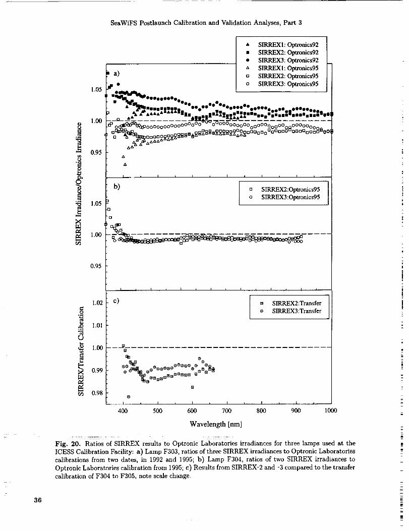
SeaWiFS Postlaunch Calibrationand ValidationAnalyses, Part 3

36

1.05

1.00

0.95t_

• _,,,i

1.05

_ 1.00

0.95

1.02

"3

1.01

,_ 1.00

_ 0.99

0.98

• SIRREX 1: Optronics92

• SIRREX2:Optronics92

• SIRREX3:Optronics92" SIRREX 1: Optronics95

a) o SIRREX2:Optronics95

• o SIRREX3:Optronics95

"_mPI,_e_pefj_ll_'eeeeeeee•

•4•'b, A-"4,4,6,.... nimlggmlllm_llll_e_:_[nmn•nnauuu•nUnnamUnmnuUUg !

_...a_ .......... _m3_ _ ..................._10(_!_)0 00000000000000 oUOOOOOooOOe_oOOOon OOr, noOOoon^_

O0 _ _0 _ _',.'u

001:__ 0O00_l_ 000_ a _ _°_(_I_I_°°°_ O00000000oOOA °°°°°°°°_OC

"1

O

"0

b)

I n I n I n I i I i I I

[] SIRREX2:Optronics95

o SIRREX3:Optronics95

I

c)

l I u I _ J i 1 I I i L,,. u

e SIRREX2:Transfere SIRREX3:Transfer

_oO oooo°ooooo_:° ,v _:_NNN_N_NN_N N m N

N

®

I , I I

400 500 600

I t I L I

700 800 900

u

1000

Wavelength [rim]

Fig. 20. Ratios of SIRREX results to Optronic Laboratories irradiances for three lamps used at the

ICESS Calibration Facility: a) Lamp F303, ratios of three SIRREX irradiances to Optronic Laboratories

calibrations from two dates, in 1992 and 1995; b) Lamp F304, ratios of two SIRREX irradiances to

Optronic Laboratories calibration from 1995; c) Results from SIRREX-2 and -3 compared to the transfercalibration of F304 to F305, note scale change.

z

m

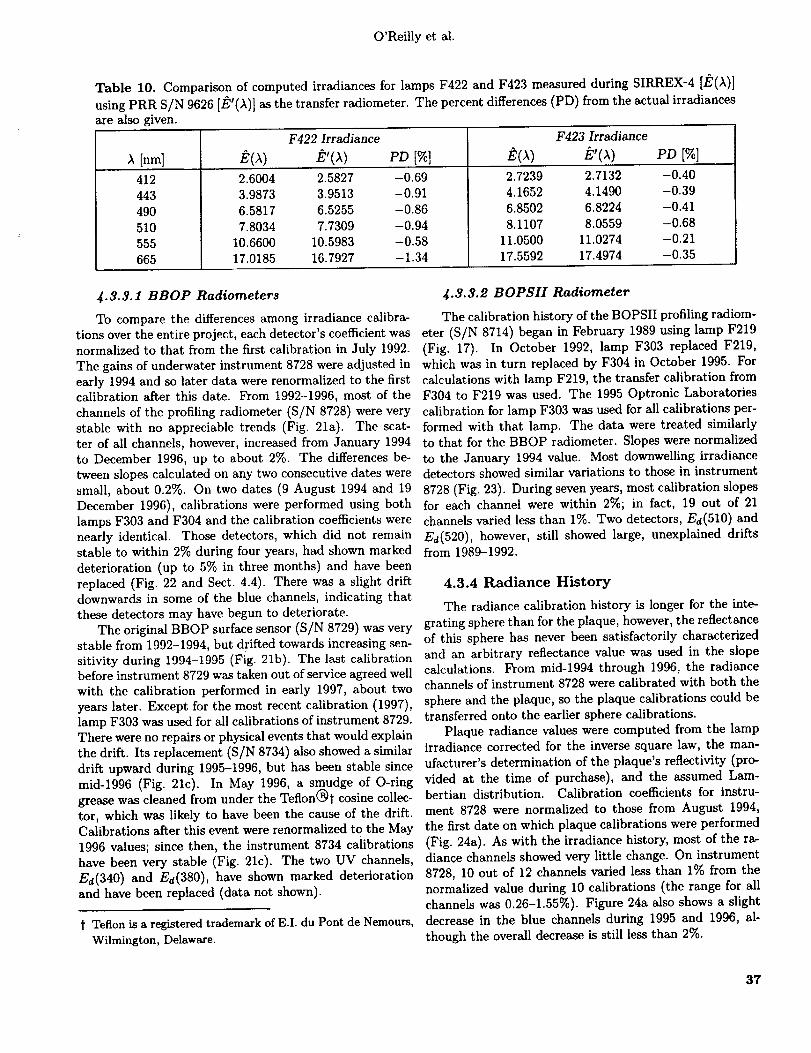
O'Reilly et al.

Table 10. Comparison of computed irradiances for lamps F422 and F423 measured during SIRREX-4 [/_(X)]

using PRR S/N 9626 [E'(A)] as the transfer radiometer. The percent differences (PD) from the actual irradiances

are also given.

F422 Irradiance F423 Irradiance

X [nm] /_(X) /_'(),) PD [%] E(X) /_'(),) PD [%]

412

443

490

510555

665

2.6004 2.5827 -0.69

3.9873 3.9513 -0.91

6.5817 6.5255 -0.86

7.8034 7.7309 -0.9410.6600 10.5983 -0.58

17.0185 16.7927 -1.34

2.7239 2.7132 -0.40

4.1652 4.1490 -0.39

6.8502 6.8224 -0.41

8.1107 8.0559 -0.68

11.0500 11.0274 -0.21

17.5592 17.4974 -0.35

4.3.3.1 BBOP Radiometers

To compare the differences among irradiance calibra-tions over the entire project, each detector's coefficient was

normalized to that from the first calibration in July 1992.

The gains of underwater instrument 8728 were adjusted inearly 1994 and so later data were renormalized to the first

calibration after this date. b-Yom 1992-1996, most of the

channels of the profiling radiometer (S/N 8728) were very

stable with no appreciable trends (Fig. 21a). The scat-ter of all channels, however, increased from January 1994

to December 1996, up to about 2%. The differences be-tween slopes calculated on any two consecutive dates were

small, about 0.2%. On two dates (9 August 1994 and 19

December 1996), calibrations were performed using bothlamps F303 and F304 and the calibration coefficients were

nearly identical. Those detectors, which did not remainstable to within 2% during four years, had shown marked

deterioration (up to 5% in three months) and have been

replaced (Fig. 22 and Sect. 4.4). There was a slight drift

downwards in some of the blue channels, indicating thatthese detectors may have begun to deteriorate.

The original BBOP surface sensor (S/N 8729) was very

stable from 1992-1994, but drifted towards increasing sen-sitivity during 1994-1995 (Fig. 21b). The last calibrationbefore instrument 8729 was taken out of service agreed well

with the calibration performed in early 1997, about two

years later. Except for the most recent calibration (1997),lamp F303 was used for all cMibrations of instrument 8729.

There were no repairs or physical events that would explain

the drift. Its replacement (S/N 8734) also showed a similardrift upward during 1995-1996, but has been stable since

mid-1996 (Fig. 21c). In May 1996, a smudge of O-ringgrease was cleaned from under the Teflon(_t cosine collec-

tor, which was likely to have been the cause of the drift.Calibrations after this event were renormalized to the May

1996 values; since then, the instrument 8734 calibrations

have been very stable (Fig. 21c). The two UV channels,

Ea(340) and Ea(380), have shown marked deteriorationand have been replaced (data not shown).

Teflon is a registered trademark of E.I. du Pont de Nemours,

Wilmington, Delaware.

4.3.3.2 BOPSII Radiometer

The calibration history of the BOPSII profiling radiom-

eter (S/N 8714) began in February 1989 using lamp F219

(Fig. 17). In October 1992, lamp F303 replaced F219,which was in turn replaced by F304 in October 1995. For

calculations with lamp F219, the transfer calibration fromF304 to F219 was used. The 1995 Optronic Laboratories

calibration for lamp F303 was used for all calibrations per-formed with that lamp. The data were treated similarly

to that for the BBOP radiometer. Slopes were normalized

to the January 1994 value. Most downwelling irradiancedetectors showed similar variations to those in instrument

8728 (Fig. 23). During seven years, most calibration slopesfor each channel were within 2%; in fact, 19 out of 21

channels varied less than 1%. Two detectors, Ed(510) and

Ed(520), however, still showed large, unexplained driftsfrom 1989-1992.

4.3.4 Radiance History

The radiance calibration history is longer for the inte-

grating sphere than for the plaque, however, the reflectanceof this sphere has never been satisfactorily characterized

and an arbitrary reflectance value was used in the slope

calculations. From mid-1994 through 1996, the radiancechannels of instrument 8728 were calibrated with both the

sphere and the plaque, so the plaque calibrations could be

transferred onto the earlier sphere calibrations.Plaque radiance values were computed from the lamp

irradiance corrected for the inverse square law, the man-

ufacturer's determination of the plaque's reflectivity (pro-

vided at the time of purchase), and the assumed Lam-bertian distribution. Calibration coefficients for instru-

ment 8728 were normalized to those from August 1994,

the first date on which plaque calibrations were performed

(Fig. 24a). As with the irradiance history, most of the ra.diance channels showed very little change. On instrument8728, 10 out of 12 channels varied less than 1% from the

normalized value during 10 calibrations (the range for all

channels was 0.26-1.55%). Figure 24a also shows a slightdecrease in the blue channels during 1995 and 1996, al-

though the overall decrease is still less than 2%.

37

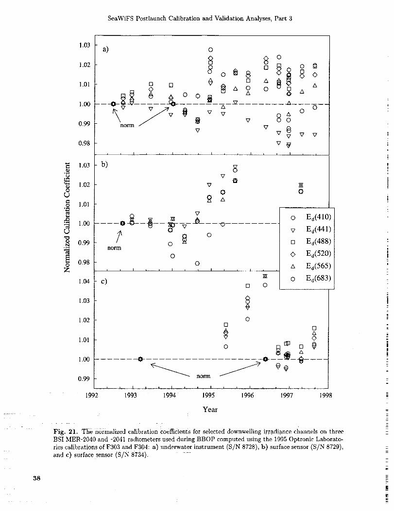
SeaWiFS Postlaunch Calibration and Validation Analyses, Part 3

38

©°_,,_

ca

8_9

O

_9

N°1,,_

OZ

1.03

1.02

1.01

1.00

0.99

0.98

1.03

1.02

1.01

1.00

0.99

0.98

1.04

1.03

1.02

1.01

l.O0

a)

[] []

norm /

i

b)

....norm

0

• i I i i | i

c)

El-

0

88e

o

V

_7

• I

o_8[]

A

AV

V

i 1 !

_ O

[] 8 o

OO

&8ov

v _7 v v

I I I I I

_7

8_7

OA

O

vA

.... _ -- -- -0

O

O. | | t i | i

[] 0

o Ed(410)

v Ea(441)

[] Ea(488)

0 Ea(520)

a Ea(565 )

0 Ed(683)

O[]

O

norm

[3AO

....

0.99

i • L L l I i i I I i I _ i l l ]

1992 1993 1994 1995 1996 1997 1998

Year

: : 77

Fig. 21. The normalized calibration Coefficients for selected downweliing irradiance channels on three

BSI MER-2040 and -2041 radiometers used during BBOP computed using the 1995 Optronic Laborato-

ries calibrations of F303 and F304: a) underwater instrument (S/N 8728), b) surface sensor (S/N 8729),

and c) surface sensor (S/N 8734).

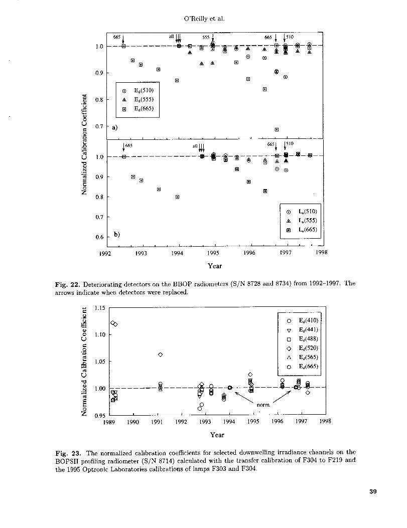
O'Reilly et al.

©

O

_9N

O

Z

i.0

0.9

0.8

0.7

1.0

0.9

0.8

0.7

665

[][] & & []

[]

a)

i

__--_

® E,_(510)

& Ed(555)

IE Ed(665)

b)

t

_-e-.-_--*--_--lg-_-_-$-_A _ _ | _

® ®

[E

I I I I .... L_ I i I I

B

[][]

[]

®

[] ®

[]

m

[]

._a__ i i i t

-_- I--_--_- -

B

® ®

®

IE

0.6

|, I i i I J __. 1 I i i I

1992 1993 1994 1995 1996 1997

t_(510)

L_(555)

I_(665) i

i ____J

1998

Year

Fig. 22. Deteriorating detectors on the BBOP radiometers (S/N 8728 and 8734) from 1992-1997. The

arrows indicate when detectors were replaced.

O

_9

O

¢}

v$

O

Z

1.15

1.10

1.05

%

1.00

<>

O Ed(410)

X7 Ed(441)

rn E_(488)

O Ea(520)

/x Ea(565)

O Ed(665)

(>

oOI I

norm

0.95 , , , t t _z______

1989 1990 1991 1992 1993 1994 1995 1996 1997 1998

Year

Fig. 23. The normalized calibration coefficients for selected downwelling irradiance channels on the

BOPSII profiling radiometer (S/N 8714) calculated with the transfer calibration of F304 to F219 and

the 1995 Optronic Laboratories calibrations of lamps F303 and F304.

39

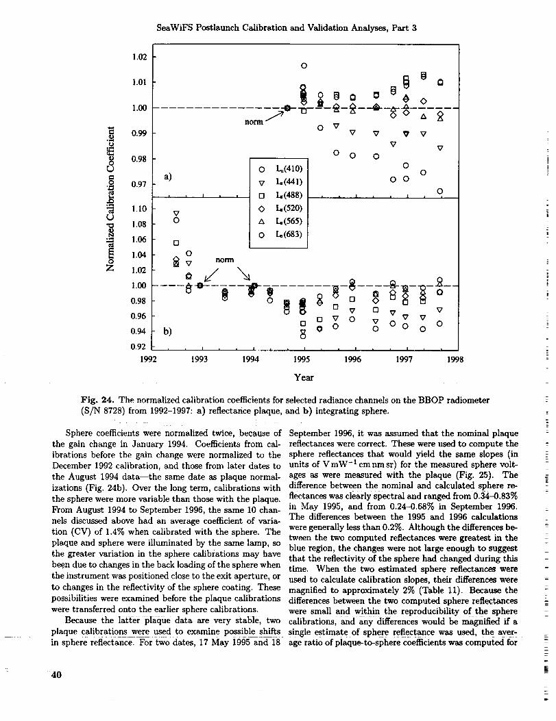
SeaWiFS Postlaunch Calibrationand ValidationAnalyses, Part 3

°¢=qo

L_

O"z_

L)

.plw

O

Z

1.02

1.01

1.00

0.99

0.98

0.97

1.10

1.08

1._

1._

1.02

1._

0.98

0.96

0._

0._

1992

a)

|

V0

r3

0_7 norm

....

b)

I , •

1993

0

no / O- §O v

v v

v

O O O

0 Lu(410)

V t.(44])

o L,(488)

0 h(520)

A L,(565)

0 I_(683)

t , I

0

0 0

• !

v

v

0

0

....

[] v n vv v

n B v 0 v 0 0 080 ° o o

I _ , 1 I I I i n I I

i994 1995 1996 1997 1998

Year

Fig. 24. The normalized calibration coefficients for

(S/N 8728) from 1992-1997: a) reflectance plaque,

Sphere coefficients were normalized twice, because of

the gain change in January 1994. Coefficients from cal-

ibrations before the gain change were normalized to the

December 1992 calibration, and those from later dates to

the August 1994 data--the same date as plaque normal-

izations (Fig. 24b). Over the long term, calibrations with

the sphere were more variable than those with the plaque.

From August 1994 to September 1996, the same 10 chan-

nels discussed above had an average coefficient of varia-

tion (CV) of 1.4% when calibrated with the sphere. The

plaque and sphere were illuminated by the same lamp, so

the greater variation in the sphere calibrations may have

been due to changes in the back loading of the sphere when

the instrument was positioned close to the exit aperture, or

to changes in the reflectivity of the sphere coating. Thesepossibilities were examined before the plaque calibrations

were transferred onto the earlier sphere calibrations.

Because the lattei plaque data are very stable, two

selected radiance channels on the BBOP radiometer

and b) integrating sphere.

September 1996, it was assumed that the nominal plaquereflectances were correct. These were used to compute the

sphere reflectances that would yield the same slopes (inunits of V roW- l cm nm sr) for the measured sphere volt-

ages as were measured with the plaque (Fig. 25). Thedifference between the nominal and calculated sphere re-fiectances was clearly spectral and ranged from 0._-0.83%

in May 1995, and from 0.24-0.68% in September 1996.The differences between the 1995 and 1996 calculations

were generally less than 0.2%. Although the differences be-tween the two computed reflectances were greatest in the

blue region, the changes were not large enough to suggestthat the reflectivity of the sphere had changed during thistime. When the two estimated sphere reflectances were

used to calculate calibration slopes, their differenc_ were

magnified to approximately 2% (Table 1i). Because thedifferences between the two computed sphere reflectances

were small and within the reproducibility of the spherecalibrations, and any differences would be magnified ff a

plaque calibrations were used to examine possible shifts single estimate of sphere reflectance was used, the aver-in sphere reflectance. For two dates, 17 May 1995 and 18 age ratio of plaque-to-sphere coefficients was computed for

4O

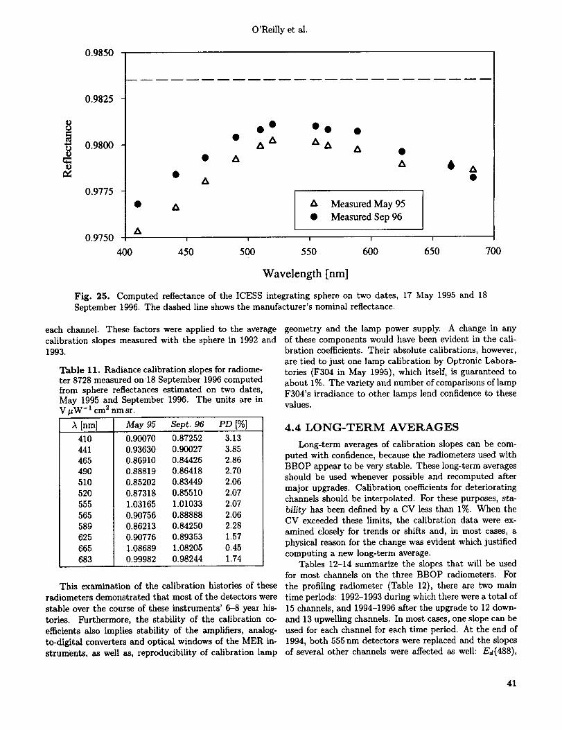
O'Reilly et al.

0.9850

0.9825

0.9800

0.9"/75

0.9750

400

• A

00 •

A Measured May 95

• Measured Sep 96

A

I I i I I

450 500 550 600 650 700

Wavelength [nm]

Fig. 25. Computed reflectance of the ICESS integrating sphere on two dates, 17 May 1995 and 18

September 1996. The dashed line shows the manufacturer's nominal reflectance.

each channel. These factors were applied to the average

calibration slopes measured with the sphere in 1992 and1993.

Table 11. Radiance calibration slopes for radiome-ter 8728 measured on'18 September 1996 computed

from sphere reflectances estimated on two dates,May 1995 and September 1996. The units are inV pW- l cm 2 nm sr.

A [nm] May 95 Sept. 96 PD [%]

410441

465

490510

520

555

565589

625

665

683

0.90070 0.87252 3.13

0.93630 0.90027 3.85

0.86910 0.84426 2.86

0.88819 0.86418 2.70

0.85202 0.83449 2.06

0.87318 0.85510 2.07

1.03165 1.01033 2.07

0.90756 0.88888 2.06

0.86213 0.84250 2.28

0.90776 0.89353 1.57

1.08689 1.08205 0.45

0.99982 0.98244 1.74

This examination of the calibration histories of these

radiometers demonstrated that most of the detectors were

stable over the course of these instruments' 6-8 year his-

tories. Furthermore, the stability of the calibration co-

efficients also implies stability of the amplifiers, analog-

to-digital converters and optical windows of the MER in-

struments, as well as, reproducibility of calibration lamp

geometry and the lamp power supply. A change in any

of these components would have been evident in the cali-bration coefficients. Their absolute calibrations, however,

are tied to just one lamp calibration by Optronic Labora-

tories (F304 in May 1995), which itself, is guaranteed toabout 1%. The variety and number of comparisons of lampF304's irradiance to other lamps lend confidence to thesevalues.

4.4 LONG-TERM AVERAGES

Long-term averages of calibration slopes can be com-

puted with confidence, because the radiometers used withBBOP appear to be very stable. These long-term averages

should be used whenever possible and recomputed after

major upgrades. Calibration coefficients for deterioratingchannels should be interpolated. For these purposes, sta-

bility has been defined by a CV less than 1%. When the

CV exceeded these limits, the calibration data were ex-

amined closely for trends or shifts and, in most cases, a

physical reason for the change was evident which justified

computing a new long-term average.Tables 12-14 summarize the slopes that will be used

for most channels on the three BBOP radiometers. For

the profiling radiometer (Table 12), there are two main

time periods: 1992-1993 during which there were a total of

15 channels, and 1994-1996 after the upgrade to 12 down-

and 13 upwelling channels. In most cases, one slope can beused for each channel for each time period. At the end of

1994, both 555 nm detectors were replaced and the slopes

of several other channels were affected as well: Ed(488),

41

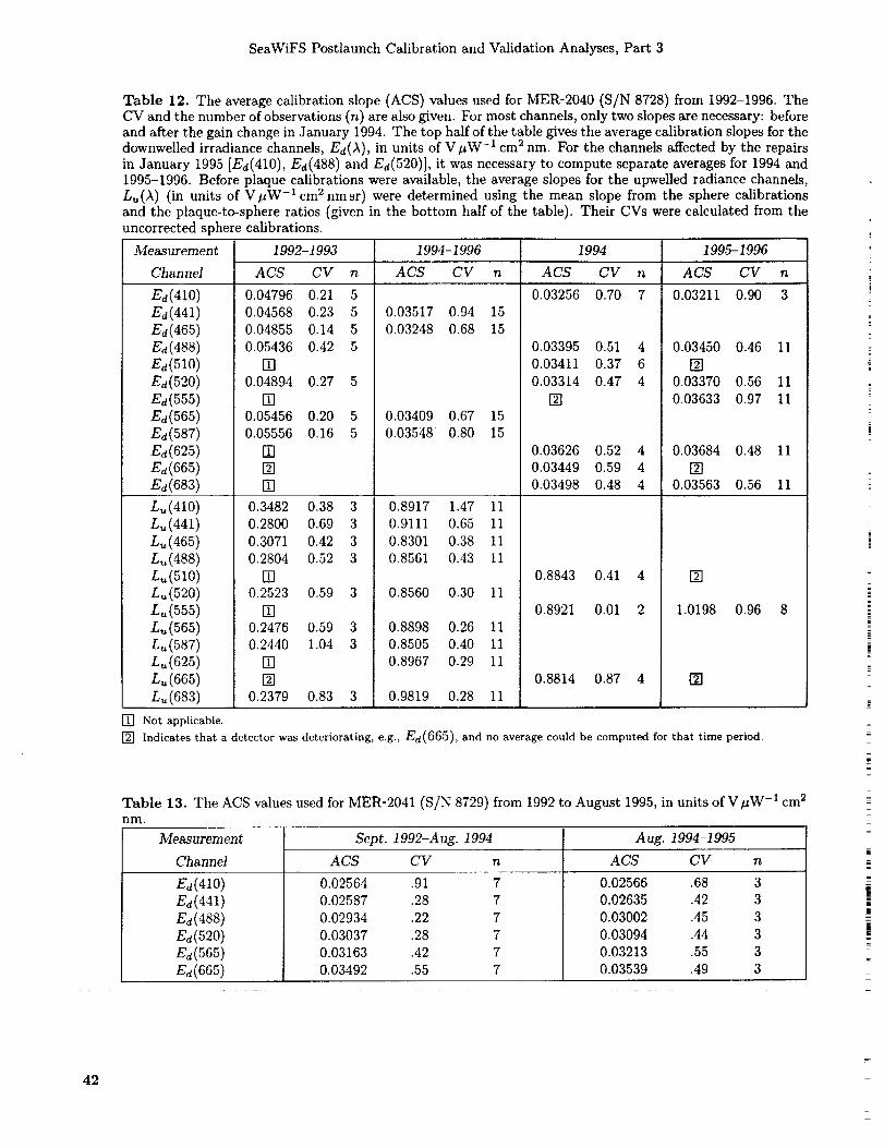
SeaWiFSPostlaunchCalibrationandValidationAnalyses,Part3

Table 12. Theaveragecalibrationslope(ACS)valuesusedfor MER-2040(S/N8728)from1992-1996.TheCVandthenumberofobservations(n)arealsogiven.Formostchannels,onlytwoslopesarenecessary:beforeandafterthegainchangeinJanuary1994.Thetophalfofthetablegivestheaveragecalibrationslopesforthedownwelledirradiancechannels,Ed(A), in units of VpW -1 cm 2 nm. For the channels affected by the repairs

in January 1995 [Ed(410), Ed(488) and Ed(520)], it was necessary to compute separate averages for 1994 and1995-1996. Before plaque calibrations were available, the average slopes for the upwelled radiance channels,

Lu(A) (in units of VpW -1 cm2nmsr) were determined using the mean slope from the sphere calibrationsand the plaque-to-sphere ratios (given in the bottom half of the table). Their CVs were calculated from theuncorrected sphere calibrations.

Measurement 1992-1993 1994-1996 1994 1995-1996

Channel A CS CV n A CS CV n A CS CV n A CS CV n

0.03256 0.70 7 0.03211 0.90 3Ed(410)E.(441)Ed(465)Ed(488)Ed(510)Ed(520)E.(555)Ed(565)E_(587)E_(625)Ed(665)Ed(683)

Lu(410)L_(441)L_(465)L_(488)L_(510)L_(520)L_(555)L_(565)L_(587)L_(625)L_(665)Lu(683)

0.04796

0.04568

0.04855

0.05436

[]0.04894

[]0.05456

0.05556

[][][]

0.21 5

0.23 5

0.14 5

0.42 5

0.27 5

0.20 5

0.16 5

0.3482 0.38 3

0.03517 0.94 15

0.03248 0.68 15

0.03409 0.67 15

0.03548 0.80 15

0:8917 -=°==1.47 °° 11

0.03395 0.51 40.03411 0.37 6

0.03314 0.47 4

[]

0.03626 O.52 4

0.03449 0.59 4

0.03498 0.48 4

0.03450 0.46 11

[]0.03370 0.56 11

0.03633 0.97 11

0.03684 0.48 11

[]0.03563 0.56 11

0.2800 0.69 3

0.3071 0.42 3

0.2804 0.52 3

[]0.2523 0.59 3

[]0.2476 0.59 3

0.2440 1.04 3

[][]

0.2379 0.83 3

0.9111 0.65 11

0.8301 0.38 110.8561 0.43 11

0.8560 0.30 11

0.8898 0.26 11

0.8505 0.40 110.8967 0.29 11

0.9819 0.28 11

0.8843 0.41 4

0.8921 0.01 2

0.8814 0.87 4

[]

1.0198

[]

0.96 8

[] Not applicable.

[] Indicates that a detector was deteriorating, e.g., Ed(665), and no average could be computed for that time period.

Table 13. The ACS values used for MER-2041 (S/N 8729) from 1992 to August 1995, in units of VpW -1 cm 2nm.

l_Ieasurement

Channel

Ed(410)

Ed(441)

Ed(488)

Ee(520)

Ed(565)

Ed(665)

Sept. 1992-Aug. 1994 Aug. 1994-1995

ACS CV n ACS CV n

0.02564 .91 7

0.02587 .28 7

0.02934 .22 7

0.03037 .28 7

0.03163 .42 7

0.03492 .55 7

0.02566 .68 3

0.02635 .42 3

0.03002 .45 3

0.03094 .44 3

0.03213 .55 3

0.03539 .49 3

42

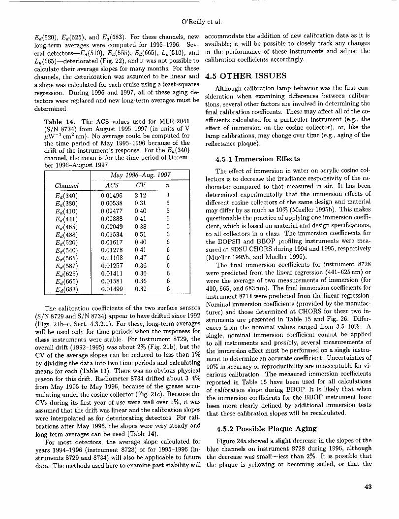
O'Reillyet al.

Ed(520), Ed(625), and Ed(683). For these channels, new

long-term averages were computed for 1995-1996. Sev-

eral detectors--Ed(510), E_(555), Ed(665), L_(510), and

L_ (665)--deteriorated (Fig. 22), and it was not possible tocalculate their average slopes for many months. For these

channels, the deterioration was assumed to be linear and

a slope was calculated for each cruise using a least-squares

regression. During 1996 and 1997, all of these aging de-

tectors were replaced and new long-term averages must bedetermined.

Table 14. The ACS values used for MER-2041

(S/N 8734) from August 1995-1997 (in units of V#W-1 cm 2 nm). No average could be computed forthe time period of May 1995-1996 because of thedrift of the instrument's response. For the Ed(340)channel, the mean is for the time period of Decem-

)er 1996-August 1997.

Channel

Ed(340)

Ed(380)Ed(410)

Ed(441)

Ed(465)

Ed(488)

Ed(520)Ed(540)

Ed(565)Ed(587)Ed(625)Ed(665)Ed(683)

May 1996-Aug. 1997

A CS CV n

0.01496 2.12 30.00538 0.31 6

0.02477 0.40 6

0.02888 0.41 6

0.02049 0.38 6

0.01534 0.51 6

0.01617 0.40 6

0.01278 0.41 6

0.01108 0.47 6

0.01257 0.36 6

0.01411 0.36 6

0.01581 0.36 6

0.01499 0.32 6

The calibration coefficients of the two surface sensors

(S/N 8729 and S/N 8734) appear to have drifted since 1992

(Figs. 21b-c, Sect. 4.3.2.1). For these, long-term averages

will be used only for time periods when the responses forthese instruments were stable. For instrument 8729, the

overall drift (1992-1995) was about 2% (Fig. 21b), but theCV of the average slopes can be reduced to less than 1%

by dividing the data into two time periods and calculating

means for each (Table 13). There was no obvious physicalreason for this drift. Radiometer 8734 drifted about 3-4%

from May 1995 to May 1996, because of the grease accu-

mulating under the cosine collector (Fig. 21c). Because the

CVs during its first year of use were well over 1%, it wasassumed that the drift was linear and the calibration slopes

were interpolated as for deteriorating detectors. For cali-

brations after May 1996, the slopes were very steady and

long-term averages can be used (Table 14).

For most detectors, the average slope calculated for

years 1994-1996 (instrument 8728) or for 1995-1996 (in-

struments 8729 and 8734) will also be applicable to futuredata. The methods used here to examine past stability will

accommodate the addition of new calibration data as it is

available; it will be possible to closely track any changes

in the performance of these instruments and adjust the

calibration coefficients accordingly.

4.5 OTHER ISSUES

Although calibration lamp behavior was the first con-

sideration when examining differences between calibra-

tions, several other factors are involved in determining the

final calibration coefficents. These may affect all of the co-

efficients calculated for a particular instrument (e.g., the

effect of immersion on the cosine collector), or, like the

lamp calibrations, may change over time (e.g., aging of the

reflectance plaque).

4.5.1 Immersion Effects

The effect of immersion in water on acrylic cosine col-

lectors is to decrease the irradiance responsivity of the ra-

diometer compared to that measured in air. It has been

determined experimentally that the immersion effects ofdifferent cosine collectors of the same design and material

may differ by as much as 10% (Mueller 1995b). This makes

questionable the practice of applying one immersion coeffi-

cient, which is based on material and design specific.ations,to all collectors in a class. The immersion coefficients for

the BOPSII and BBOP profiling instruments were mea-sured at SDSU CHORS during 1994 and 1995, respectively

(Mueller 1995b, and Mueller 1996).The final immersion coefficients for instrument 8728

were predicted from the linear regression (441-625 rim) orwere the average of two measurements of immersion (for

410, 665, and 683 nm). The final immersion coefficients for

instrument 8714 were predicted from the linear regression.

Nominal immersion coefficients (provided by the manufac-

turer) and those determined at CHORS for these two in-struments are presented in Table 15 and Fig. 26. Differ-ences from the nominal values ranged from 3.5-10%. A

single, nominal immersion coefficient cannot be appliedto all instruments and possibly, several measurements of

the immersion effect must be performed on a single instru-ment to determine an accurate coefficient. Uncertainties of

10% in accuracy or reproducibility are unacceptable for vi-carious calibration. The measured immersion coefficients

reported in Table 15 have been used for all calculationsof calibration slope during BBOP. It is likely that whenthe immersion coefficients for the BBOP instrument have

been more clearly defined by additional immersion tests

that these calibration slopes will be recalculated.

4.5.2 Possible Plaque Aging

Figure 24a showed a slight decrease in the slopes of theblue channels on instrument 8728 during 1996, althoughthe decrease was small--less than 2%. It is possible that

the plaque is yellowing or becoming soiled, or that the

43

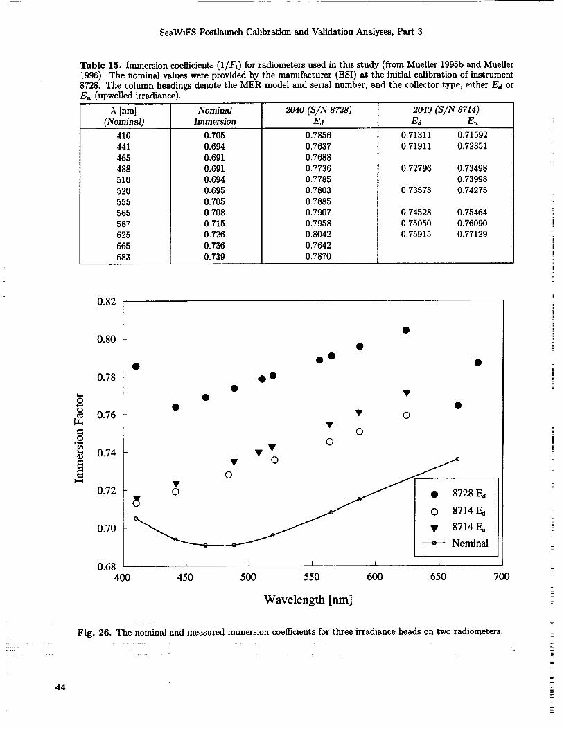
SeaWiFS Postlaunch Calibrationand ValidationAnalyses,Part 3

Table 15. Immersion coefficients(I/F,)forradiometersused inthisstudy (from Mueller 1995b and Mueller

1996). The nominal valueswere provided by the manufacturer (BSI) at the initialcalibrationof instrument8728. The column headings denote the MER model and serialnumber, and the collectortype,eitherEd or

Eu (upwelledirradiance).

A [nm] Nominal 2040 (S/N 8728) 2040 (SIN 8714)

(Nominal) Immersion E_ E_ E_,

410

441

465

488

510

520

555

565

587

625

665

683

0.705

0.694

0.691

0.691

0.694

0.695

0.705

0.708

0.7150.726

0.736

0.739

0.7856

0.7637

0.76880.7736

0.7785

0.78030.7885

0.7907

0.7958

0.8042

0.7642

0.7870

0.71311 0.71592

0.71911 0.72351

0.72796 0.73498

0.73998

0.73578 0.74275

0.74528 0.75464

0.75050 0.76090

0.75915 0.77129

0.82

0.80

0.78

_ 0.76

i 0.74

0.72

0.70

00

0

• v_ O

0 __7 --

28 Ed 1

O 8714 N

V 8714 Eu

Nominal

I i I I0.68 I400 450 500 550 600 650 700

Wavelength [nm]

Fig. 26. The nominal and measured immersion coefficients for three irradiance heads on two radiometers.

44

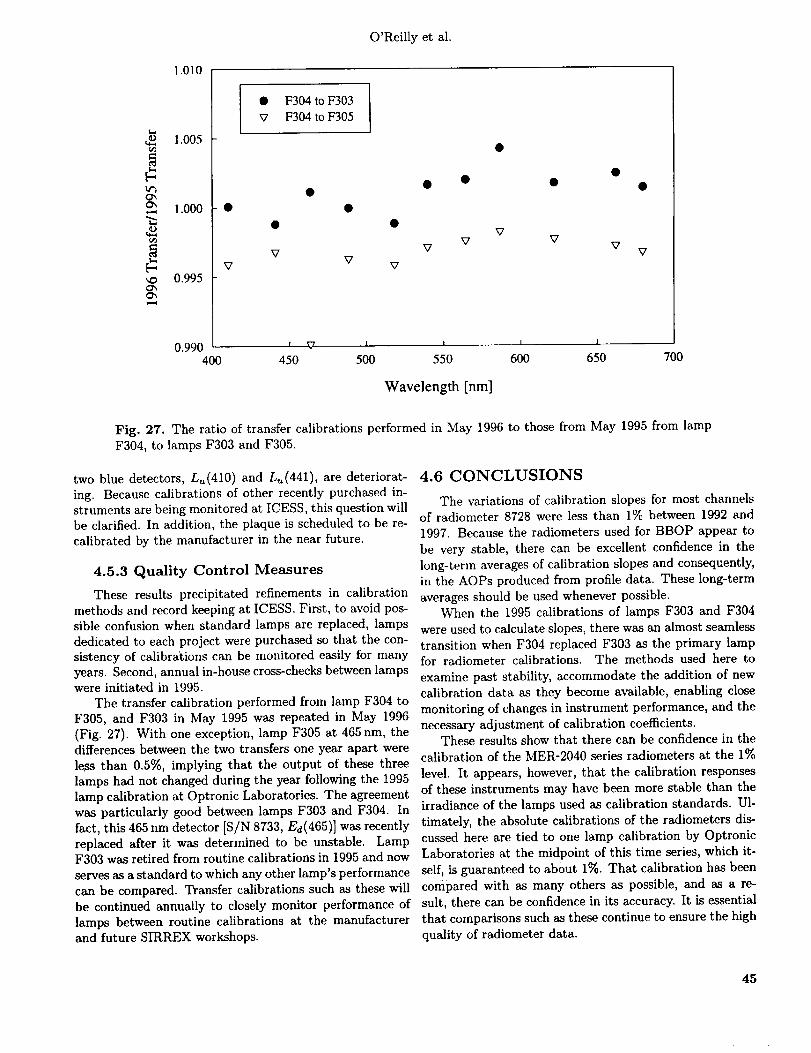
t_

t-,

o_

_D

1.010

1.005

1.000 @

_70.995

0.990400

O'Reilly et al.

I• F304toF303 ]

I_7 F304toF305

vv

v

v

f _ i i i I

450 500 550 600 650

Wavelength [nm]

700

Fig. 27. The ratio of transfer calibrations performed in May 1996 to those from May 1995 from lampF304, to lamps F303 and F305.

two blue detectors, L_(410) and L_,(441), are deteriorat-ing. Because calibrations of other recently purchased in-

struments are being monitored at ICESS, this question willbe clarified. In addition, the plaque is scheduled to be re-

cMJbrated by the manufacturer in the near future.

4.5.3 Quality Control Measures

These results precipitated refinements in calibration

methods and record keeping at ICESS. First, to avoid pos-

sible confusion when standard lamps are replaced, lamps

dedicated to each project were purchased so that the con-sistency of calibrations can be monitored easily for many

years. Second, annual in-house cross-checks between lampswere initiated in 1995.

The transfer calibration performed from lamp F304 to

F305, and F303 in May 1995 was repeated in May 1996(Fig. 27). With one exception, lamp F305 at 465 nm, the

differences between the two transfers one year apart were

less than 0.5%, implying that the output of these three

lamps had not changed during the year following the 1995lamp calibration at Optronic Laboratories. The agreement

was particularly good between lamps F303 and F304. In

fact, this 465 nm detector [S/N 8733, Ed(465)] was recently

replaced after it was determined to be unstable. LampF303 was retired from routine calibrations in 1995 and now

serves as a standard to which any other lamp's performance

can be compared. Transfer calibrations such as these will

be continued annually to closely monitor performance of

lamps between routine calibrations at the manufacturerand future SIRREX workshops.

4.6 CONCLUSIONS

The variations of calibration slopes for most channelsof radiometer 8728 were less than 1% between 1992 and

1997. Because the radiometers used for BBOP appear to

be very stable, there can be excellent confidence in thelong-term averages of calibration slopes and consequently,

in the AOPs produced from profile data. These long-term

averages should be used whenever possible.When the 1995 calibrations of lamps F303 and F304

were used to calculate slopes, there was an almost seamless

transition when F304 replaced F303 as the primary lampfor radiometer calibrations. The methods used here to

examine past stability, accommodate the addition of new

calibration data as they become available, enabling close

monitoring of changes in instrument performance, and the

necessary adjustment of calibration coefficients.These results show that there can be confidence in the

calibration of the MER-2040 series radiometers at the 1%

level. It appears, however, that the calibration responses

of these instruments may have been more stable than the

irradiance of the lamps used as calibration standards. Ul-

timately, the absolute calibrations of the radiometers dis-

cussed here are tied to one lamp calibration by Optronic

Laboratories at the midpoint of this time series, which it-

self, is guaranteed to about 1%. That calibration has been

compared with as many others as possible, and as a re-

suit, there can be confidence in its accuracy. It is essential

that comparisons such as these continue to ensure the high

quality of radiometer data.

45

46

ALOHA

ACS

AI9901

AMT

AOP

BATS

BBOP

Ber95

Ber96

BOPSII

BSI

CalCOFI

CARIACO

CB-MAB

CDOM

CHORS

COARE

COASTS

CoBOPCSC

CV

CVT

CZCS

DARR

EcoHAB

EqPac

FEL

FL-Cuba

FWHM

GOM

GoA97

GSFC

HOT

HPLC

ICESS

IDL

JES9906

JGOFS

Lab96

Lab97

Lab98

LTER

MCP

MBARI

MBR

MER

MERIS

MF0796

MOCE

MODIS

SeaWiFS Postlaunch Calibration and Validation Analyses, Part 3

GLOSSARY

A Long-term Oligotrophic Habitat Assessment

[the Hawaii Ocean Time-series (HOT) deep-water station located about 1001on north of

Oahu, Hawaii].Average Calibration Slope

Atlantic-Indian Ocean Cruise, 1999

Atlantic Meridional Transect

Apparent Optical Properties

Bermuda Atlantic Time Series

Bermuda BioOptics Project

Bering Sea Cruise, 1995

Bering Sea Cruise, 1996

Bio-Optical Profiling System II (second gen-eration)

Biospherical Instruments, Inc.

California Cooperative Oceanic Fisheries In-

vestigationCarbon Retention in a Colored Ocean

Chesapeake Bay-Middle Atlantic Bight

Colored Dissolved Organic Matter

Center for Hydro-Optics and Remote Sensing

Coupled Ocean Atmosphere Response Exper-iment

Coastal Atmosphere and Sea Time Series

Coastal Benthic Optical Properties (Bahamas)

Coastal Service Center, (NOAA, SC)Coefficient of Variation

Calibration and Validation Team

Coastal Zone Color Scanner

Data Analysis Round-Robin (workshop)

Ecology of Harmful Algal Blooms

Equatorial Pacific

Not an acronym, but a type of irradiance lampdesignator.Florida-Cuba cruise.

Full-Width at Half-Maximum

Gulf of Maine

Gulf of Alaska Cruise, 1997

Goddard Space Flight Center

Hawaii Ocean Time-series

High Performance Liquid Chromatography

Institute for Computational Earth System Sci-ence

Interactive Data Language

Japan East Sea Cruise, 1999-06

Joint Global Ocean Flux Study

Labrador Sea Cruise, 1996

Labrador Sea Cruise, 1997

Labrador Sea Cruise, 1998

Long Term Ecological Research

Modified Cubic Polynomial

Monterey Bay Aquarium Research InstituteMaximum Band Ratio

Marine Environmental Radiometer

Medium Resolution Imaging Spectrometer

R/V Miller Freeman Cruise, 1996-07

Marine Optical Characterization Experiment

Moderate Resolution Imaging Spectroradiom-eter

NABE

NASA

NEGOM

NIST

NOAA

OC2

OC2v2

OC4

OC4v2

OC4v4

OCTS

ORINOCO

PD

PRR

RED9503

Res94

Res95-2

Res96

Res98

RMS

ROAVERRS

SDSU

SeaBAM

SeaWiFS

SIMBIOS

SIRREX

SIRREX- 1

SIRREX-2

SIRREX-3

SIRREX-4

SMAB

S/NSNR

SPO

TOGA

TOTO

UCSB

URL

UVA

WOCE

North Atlantic Bloom Experiment

National Aeronautics and Space Administra-tion

Northeast Gulf of Mexico

National Institute for Standards and Technol-

ogy

National Oceanic and Atmospheric Adminis-tration

Ocean Chlorophyll 2 algorithmOC2 version 2.

Ocean Chlorophyll 4 algorithm0C4 version 2.

OC4 version 4.

Ocean Color and Temperature Scanner

Orinoco River Plume

Percent Difference

Profiling Reflectance Radiometer

Red Tide Cruise, 1995-03

Resolute Cruise, 1994Resolute Cruise, 1995Resolute Cruise, 1996

Resolute Cruise, 1998Root Mean Square

Research on Ocean-Atmosphere Variability

and Ecosystem Response in the Ross Sea

San Diego State UniversitySeaWiFS Bio-optical Algorithm Mini-

workshop

Sea-viewing Wide Field-of-view Sensor

Sensor Intercomparison and Merger for Bio-

logical and Interdisciplinary Oceanic Studies

SeaWiFS Intercalibration Round-Robin Ex-

periment

The first SIRREX, July 1992.

The second SIRREX, June 1993.

The third SIRREX, September 1994.

The fourth SIRREX, May 1995.

Southern Mid-Atlantlc BightSerial number

Signal-to-Noise Ratio

SeaWiFS Project Office

Tropical Ocean Global Atmosphere

Tongue of the Ocean study (Bahamas)

University of California, Santa Barbara

Universal Resource Locator

Ultraviolet-A

World Ocean Circulation Experiment

SYMBOLS

a Absorption coefficient.A Coefficient.

aw Absorption coefficient for pure water.

b Intercept.

B Coefficient.

bb Backscattering coefficient.

b_ Backscattering coefficient for pure water.

Co Chlorophyll a concentration.

Co In situ chlorophyll a concentration.

Z

O'Reilly et al.

Irradiance measured during SIRREX-4.

Irradiance measured using a PRR as the transfer

radiometer.

Downwelled spectral irradiance.

Upwelled spectral irradiance.

f Function.

FI Immersion coefficient.

K(490)

K,_(A)

L_(z,_)Lw()_)

Lw()_l)

Lw(,k2)

Diffuse attenuation coefficient at 490 nm.

Diffuse attenuation coefficient for pure water.

Upwelled spectral radiance.

Spectral water-leaving radiance.

Water-leaving radiance for wavelength A1.

Water-leaving radiance for wavelength _2.

m Slope.

n Number of observations.

N Number of data sets.

NF Number of fluorometric chlorophyll a sets.

NH Number of HPLC chlorophyll a sets.

R 2 Squared correlation coefficient.

R49oR2 loglo( $55)-

10 _R 490R2s glok 0551, see Rac, where the argument of the log-

arithm is a shorthand representation for the maxi-

mum of the three values. In an expression such as

R2s, the numerical part of the subscript refers to the

number of bands used, and the letter denotes a code

for the specific satellite sensors [S is SeaWiFS, M is

the Moderate Resolution Imaging Spectroradiome-

ter (MODIS), O is the Ocean Color and Tempera-

ture Scanner (OCTS), E is the Medium Resolution

Imaging Spectrometer (MERIS), and C is CZCS].

• tR443 R52O'tR3c loglo_ 000 > 5sol,443 R490 R51O_/LiE loglo(Rss0 > 5e0 > s60), see Rsc.

l tR443 R 49° R s20_'R40 Oglot, 560 > 500 > 5651,see R3c.

• XR443 D49o RSlO_R4s loglo( $ss > ,_s55 > s50), see R3c.

R_ Rrs ratio constructed from band A divided by band

B.

Rrs Remote sensing reflectance.

Rr_ In situ remote sensing reflectance.

/_r8 Interpolated remote sensing reflectance.

R _' A compact notation for the Rr_(Ai)/Rrs(Aj) bandAj

ratio.

x The abscissa.

y The ordinate.

z Depth.

7_ log(C_).

Wavelength.

a Standard deviation.

REFERENCES

Austin, R.W., and Petzold, T., 1981: The determination of

the diffuse attenuation coefficient of sea water using the

Coastal Zone Color Scanner. Oceanography from Space,

J.F.R. Gower, Ed., Plenum Press, 239-256.

Evans, R.H., and H.R. Gordon, 1994: Coastal zone color scan-

ner "system calibration": A retrospective examination, J.

Ceophys. Res., 99, 7,293-7,307.

Firestone, E.R., and S.B. Hooker, 1998: SeaWiFS Prelaunch

Technical Report Series Final Cumulative Index. NASA

Tech. Memo. 1998-I0_566, Vol. 43, S.B. Hooker and E.R.

Firestone, Eds., NASA Goddard Space Flight Center,

Greenbelt, Maryland, 4-8.

Gordon, H.R., and W.R. McCluney, 1975: Estimation of the

depth of sunlight penetration in the sea for remote sensing.

Appl. Opt., 14, 413-416.

_, and K. Ding, 1992: Self-shading of in-water optical in-

struments, Limnol. Oceanogr., 37, 491-500.

--, and M. Wang, 1994: Retrieval of water-leaving radiance

and aerosol optical thickness over the oceans with Sea-

WiFS: A preliminary algorithm, Appl. Opt., 33, 443-452.

Gregg, W.W., and R.H. Woodward, 1998: Improvements in

high frequency ocean color observations: Combining datafrom SeaWiFS and MODIS, IEEE Trans. Geosci. Remote

Sens., 36, 1,350-1,353.

Johnson, B.C., S.S. Bruce, E.A. Early, J.M. Houston, T.R.

O'Brian, A. Thompson, S.B. Hooker, and J.L. Mueller,1996: The Fourth SeaWiFS Intercalibration Round-Robin

Experiment (SIRREX-4), May 1995. NASA Tech. Memo.

10_566, Vol. 37, S.B. Hooker and E.R. Firestone, Eds.,

NASA Goddard Space Flight Center, Greenbelt, Mary-

land, 65 pp.

Kahru, M., and B.G. Mitchell, 1998a: Spectral reflectance and

absorption of a massive red tide off Southern California. J.

Geophys. Res., 103, 21,601-21,609.

, and _, 1998b: Evaluation of instrument self-shadingand environmental errors on ocean color algorithms. Proc.

Ocean Optics XIV, Kona, Hawaii, S. Ackleson and J.

Campbell, Eds., [Available on CD-ROM.]

Maritorena, S., and J.E. O'Reilly, 2000: OC2v2: "Update on

the initial operational SeaWiFS chlorophyll a algorithm."

In: O'Reilly, J.E., and 24 Coauthors, 2000: SeaWiFS Post-

launch Calibration and Validation Analyses, Part 3. NASA

Tech. Memo. 2000-206892, Vol. 11, S.B. Hooker and E.R.

Firestone, Eds., NASA Goddard Space Flight Center,

Greenbelt, Maryland, 3-8.

McClain, C.R., 2000: "SeaWiFS postlaunch calibration and

validation overview." In: McClain, C.R., E.J. Ainsworth,

R.A. Barnes, R.E. Eplee, Jr., F.S. Patt, W.D. Robinson,

M. Wang, and S.W. Bailey, SeaWiFS Postlaunch Cali-

bration and Validation Analyses, Part 1. NASA Tech.

Memo. 2000-206892, Vol. 9, S.B. Hooker and E,R. Fire-

stone, Eds., NASA Coddard Space Flight Center, Green-

belt, Maryland, 4-12.

47

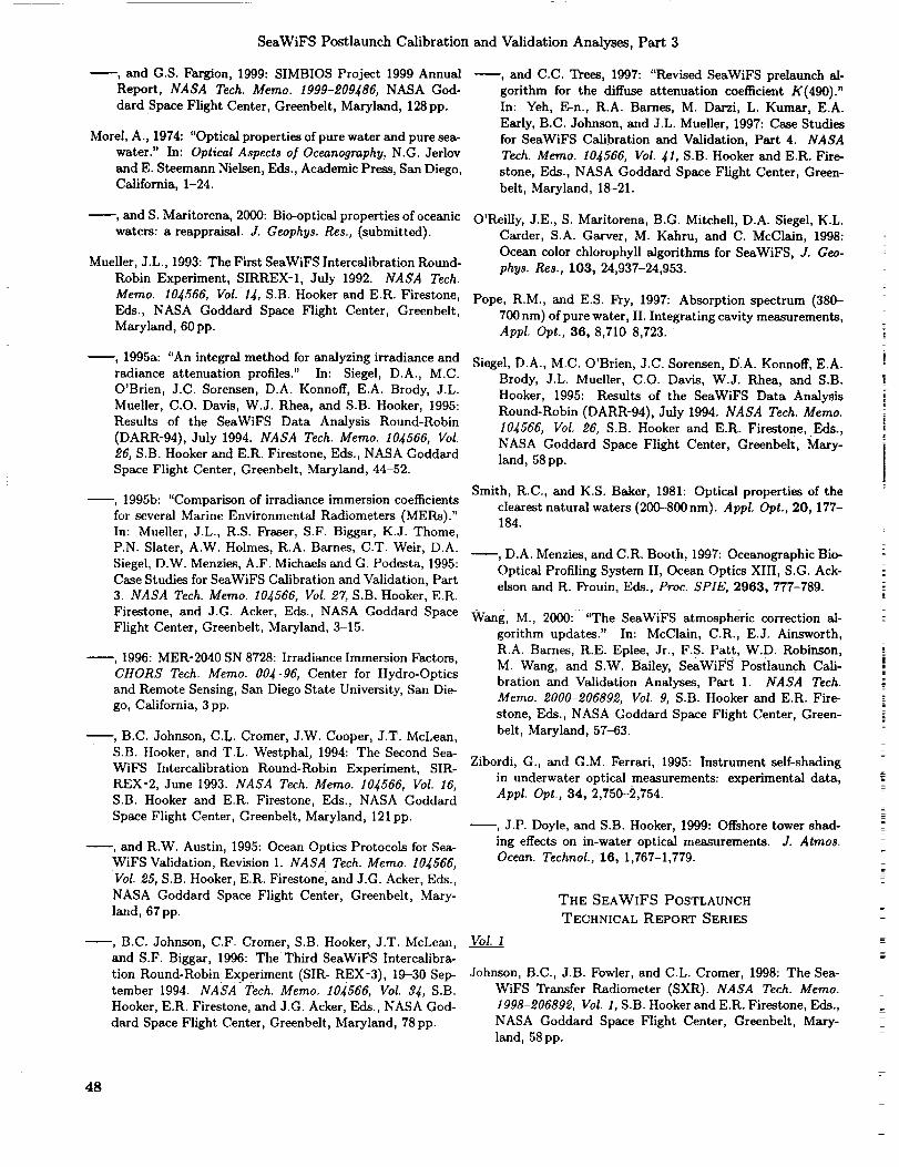
SeaWiFS Postlaunch Calibration and Validation Analyses, Part 3

, and G.S. Fargion, 1999: SIMBIOS Project 1999 Annual

Report, NASA Tech. Memo. 1999-209486, NASA God-

dard Space Flight Center, Greenbelt, Maryland, 128pp.

Morel, A., 1974: "Optical properties of pure water and pure sea-

water." In: Optical Aspects of Oceanography, N.G. Jerlov

and E. Steemann Nielsen, Eds., Academic Press, San Diego,

California, 1-24.

_, and C.C. Trees, 1997: "Revised SeaWiFS prelannch al-

gorithm for the diffuse attenuation coefficient K(490)."

In: Yeh, F_,-n., R.A. Barnes, M. Darzi, L. Kumar, E.A.

Early, B.C. Johnson, and J.L. Mueller, 1997: Case Studies

for SeaWiFS Calibration and Validation, Part 4. NASA

Tech. Memo. 104566, Vol. 41, S.B. Hooker and E.R. Fire-

stone, Eds., NASA Goddard Space Flight Center, Green-

belt, Maryland, 18-21.

_, and S. Maritorena, 2000: Bio-optical properties of oceanic

waters: a reappraisal. J. Geophys. Res., (submitted).

Mueller, J.L., 1993: The First SeaWiFS Intercalibration Round-

Robin Experiment, SIRREX-1, July 1992. NASA Tech.

Memo. 104566, Vot. 14, S.B. Hooker and E.R. Firestone,

Eds., NASA Goddard Space Flight Center, Greenbelt,

Maryland, 60pp.

, 1995a: "An integral method for analyzing irradiance and

radiance attenuation profiles." In: Siegel, D.A., M.C.

O'Brien, J.C. Sorensen, D.A. Konnoff, E.A. Brody, J.L.

Mueller, C.O. Davis, W.J. Rhea, and S.B. Hooker, 1995:

Results of the SeaWiFS Data Analysis Round-Robin

(DARR-94), July 1994. NASA Tech. Memo. 104566, Vol.

26, S.B. Hooker and E.R. Firestone, Eds., NASA Goddard

Space Flight Center, Greenbelt, Maryland, 44-52.

, 1995b: "Comparison of irradiance immersion coefficients

for several Marine Environmental Radiometers (MERs)."

In: Mueller, J.L., R.S. Fraser, S.F. Biggar, K.J. Thome,

P.N. Slater, A.W. Holmes, R.A. Barnes, C.T. Weir, D.A.

Siegel, D.W. Menzies, A.F. Michaels and G. Podesta, 1995:

Case Studies for SeaWiFS Calibration and Validation, Part

3. NASA Tech. Memo. 104566, Vol. 27, S.B. Hooker, E.R.

Firestone, and J.G. Acker, Eds., NASA Goddard Space

Flight Center, Greenbelt, Maryland, 3-15.

, 1996:MER-2040 SN 8728: Irradiance Immersion Factors,

CHORS Tech. Memo. 004-96, Center for Hydro-Optics

and Remote Sensing, San Diego State University, San Die-

go, California, 3 pp.

, B.C. Johnson, C.L. Cromer, J.W. Cooper, J.T. McLean,

S.B. Hooker, and T.L. Westphal, 1994: The Second Sea-

WiFS Intercalibration Round-Robin Experiment, SIR-

REX-2, June 1993. NASA Tech. Memo. 104566, Vot. 16,

S.B. Hooker and E.R. Firestone, Eds., NASA Goddard

Space Flight Center, Greenbelt, Maryland, 121 pp.

_, and R.W. Austin, 1995: Ocean Optics Protocols for Sea-

WiFS Validation ' Revision 1. NASA Tech. Memo. 104566,

'VoL 25, S.B. Hooker, E.R. Firestonel and J.G. Acker, Eds.,

NASA Goddard Space Flight Center, Greenbelt, Mary-

land, 67 pp.

_, B.C. Johnson, C.F. Cromer, S.B. Hooker, J.T. McLean,

and S.F. Biggar, 1996: TheThird SeaWiFS Intercalibra-

tion Round-Robin Experiment (SIR- REX-3), 19-30 Sep-

tember 1994. NASA Tech. Memo. 104566, Vol. 3J, S.B.

Hooker, E.R. Firestone, and J.G. Acker, Eds., NASA God-

dard Space Flight Center, Greenbelt, Maryland, 78 pp.

O'Reilly, J.E., S. Maritorena, B.G. Mitchell, D.A. Siegel, K.L.

Carder, S.A. Garver, M. Kahru, and C. McClain, 1998:

Ocean color chlorophyll algorithms for SeaWiFS, J. Geo-

phys. Res., 103, 24,937-24,953.

Pope, R.M., and E.S. Fry, 1997: Absorption spectrum (380-

700 nm) of pure water, II. Integrating cavity measurements,

Appl. Opt., 36, 8,710-8,723.

Siegel, D.A., M.C. O'Brien, J.C. Sorensen, D.A. Konnoff, E.A.

Brody, J.L. Mueller, C.O. Davis, W.J. Rhea, and S.B.

Hooker, 1995: Results of the SeaWiFS Data Analysis

Round-Robin (DARR-94), July 1994. NASA Tech. Memo.

104566, Vol. 26, S.B. Hooker and E.R. Firestone, Eds.,

NASA Goddard Space Flight Center, Greenbelt, Mary-

land, 58 pp.

Smith, R.C., and K.S. Baker, 1981: Optical properties of the

clearest natural waters (200-800 nm). Appl. Opt., 20, 177-184.

_, D.A. Menzies, and C.R. Booth, 1997: Oceanographic Bio-

Optical Profiling System II, Ocean Optics XIII, S.G. Ack-

elson and R. Prouin, Eds., Proc. SPIE, 2963, 777-789.

Wangl M., 2000: "The SeaWiFS atmospheric correction al-

gorithm updates." In: McClain, C.R., E.J. Ainsworth,

R.A. Barnes, R.E. Eplee, Jr., F.S. Patt, W.D. Robinson,

M. Wang, and S.W. Bailey, SeaWil_$ Postlaunch Cali-

bration and Validation Analyses, Part 1. NASA Tech.

Memo. 2000-206892, Vol. 9, S.B. Hooker and E.R. Fire-

stone, Eds., NASA Goddard Space Flight Center, Green-

belt, Maryland, 57-63.

Zibordi, G., and G.M. Ferrari, 1995: Instrument self-shading

in underwater optical measurements: experimental data,

Appl. Opt., 34, 2,750-2,754.

_, J.P. Doyle, and S.B. Hooker, 1999: Offshore tower shad-

ing effects on in-water optical measurements. J. Atmos.

Ocean. Technol., 16, 1,767-1,779.

THE SEAW1FS POSTLAUNCH

TECHNICAL REPORT SERIES

Vol. I

Johnson, B.C., J.B. Fowler, and C.L. Cromer, 1998: The Sea-

WiFS Transfer Radiometer (SXR). NASA Tech. Memo.

1998-206892, Vol. 1, S.B. Hooker and E.R. Firestone, Eds.,

NASA Goddard Space Flight Center, Greenbelt, Mary-

land, 58 pp.

48

O'Reillyetal.

Vol. 2 Vol. 7

Aiken, J., D.G. Cummings, S.W. Gibb, N.W. Rees, R. Woodd-

Walker, E.M.S. Woodward, J. Woolfenden, S.B. Hooker,

J-F. Berthon, C.D. Dempsey, D.J. Suggett, P. Wood, C.Donlon, N. Gonz_lez-Ben_tez, I. Huskin, M. Quevedo, R.

Barciela-Fernandez, C. de Vargas, and C. McKee, 1998:

AMT-5 Cruise Report. NASA Tech. Memo. 1998-206892,

Vol. 2, S.B. Hooker and E.R. Firestone, Eds., NASA God-

dard Space Flight Center, Greenbelt, Maryland, l l3pp.

Vol. 3

Hooker, S.B., G. Zibordi, G. Lazin, and S. McLean, 1999:

The SeaBOARR-98 Field Campaign. NASA Tech. Memo.

1999-206892, Vol. 3, S.B. Hooker and E.R. Firestone, Eds.,

NASA Goddard Space Flight Center, Greenbelt, Mary-

land, 40 pp.

Vol. 4

Johnson, B.C., E.A. Early, R.E. Eplee, Jr., R.A. Barnes, and

R.T. Caffrey, 1999: The 1997 Prelaunch Radiometric Cal-

ibration of SeaWiFS. NASA Tech. Memo. 1999-206892,

Vol. 4, S.B. Hooker and E.R. Firestone, Eds., NASA God-

dard Space Flight Center, Greenbelt, Maryland, 51 pp.

Vol. 5

Barnes, R.A., R.E. Eplee, Jr., S.F. Biggar, K.J. Thome, E.F.

Zalewski, P.N. Slater, and A.W. Holmes 1999: The Sea-

WiFS Solar Radiation-Based Calibration and the Transfer-

to-Orbit Experiment. NASA Tech. Memo. 1999-206892,

Vol. 5, S.B. Hooker and E.R. Firestone, Eds., NASA God-

dard Space Flight Center, 28 pp.

Vol. 6.

Firestone, E.R., and S.B. Hooker, 2000: SeaWiFS Postlannch

Technical Report Series Cumulative Index: Volumes 1-5.

NASA Tech. Memo. 2000-206892, Vol. 6, S.B. Hooker and

E.R. Firestone, Eds., NASA Goddard Space Flight Center,

Greenbelt, Maryland, 14 pp.

Johnson, B.C., H.W. Yoon, S.S. Bruce, P-S. Shaw, A. Thomp-

son, S.B. Hooker, R.E. Eplee, Jr., R.A. Barnes, S. Mar-

itorena, and J.L. Mueller, 1999: The Fifth SeaWiFS In-

tercalibration Round-Robin Experiment (SIRREX-5), July

1996. NASA Tech. Memo. 1999-_06892, Vol. 7, S.B.

Hooker and E.R. Firestone, Eds., NASA Goddard Space

Flight Center, 75 pp.

Vol. 8

Hooker, S.B., and G. Lazin, 2000: The SeaBOARR-99 Field

Campaign. NASA Tech. Memo. 2000-206892, Vol. 8, S.B.

Hooker and E.R. Firestone, Eds., NASA Goddard Space

Flight Center, 46 pp.

Vol. 9

McClain, C.R., E.J. Ainsworth, R.A. Barnes, R.E. Eplee, Jr.,

F.S. Patt, W.D. Robinson, M. Wang, and S.W. Bailey,2000: SeaWiFS Postlaunch Calibration and Validation

Analyses, Part 1. NASA Tech. Memo. 2000-206892, Vol.

9, S.B. Hooker and E.R. Firestone, Eds., NASA Goddard

Space Flight Center, 82 pp.

Vol. 10

McClain, C.R., R.A. Barnes, R.E. Eplee, Jr., B.A. Franz, N.C.

Hsu, F.S. Patt, C.M. Pietras, W.D. Robinson, B.D. Schie-

ber, G.M. Schmidt, M. Wang, S.W. Bailey, and P.J. Wer-

dell, 2000: SeaWiFS Postlaunch Calibration and Valida-

tion Analyses, Part 2. NASA Tech. Memo. 2000-206892,

Vol. 10, S.B. Hooker and E.R. Firestone, Eels., NASA God-

dard Space Flight Center, 57 pp.

Vol. 11

O'Reilly, J.E., and 24 Coauthors, 2000: SeaWiFS Postlaunch

Calibration and Validation Analyses, Part 3. NASA Tech.

Memo. 2000-206892, Vol. 11, S.B. Hooker and E.R. Fire-

stone, Eds., NASA Goddard Space Flight Center, 49 pp.

49

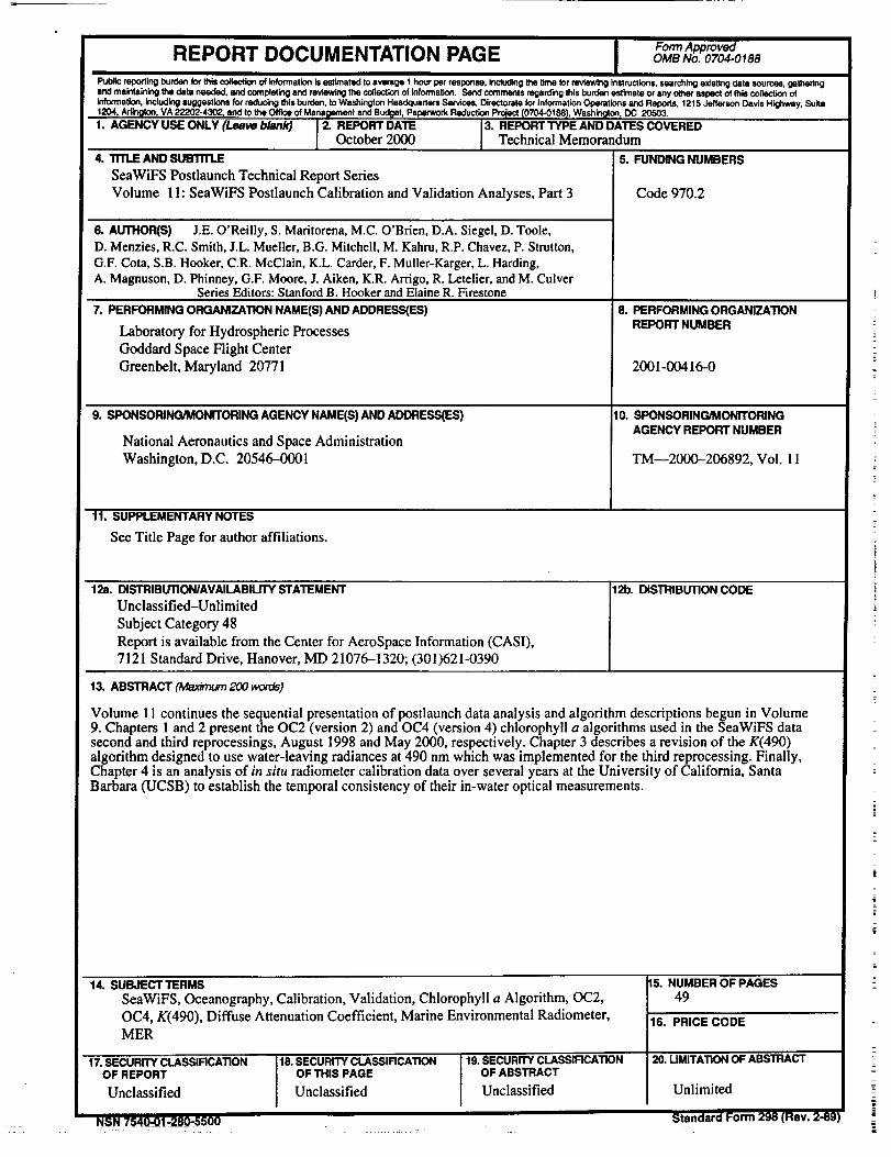
FormApprovedREPORT DOCUMENTATION PAGE OMBNo. 0704-0188

Public reporting burden k_" this collection of information Is estimated to ave_age 1 hour per response, including the time for reviewing Instructions, searching existing data sources, gathering

and maintaining the data needed, and completing and revk_ the collection of information. Send comments regarding this burden estimate or any other aspect of this oo_ctlon of

information, Including suggestk)ns for reducing this burden, to Washington Headquarters Services, Directorate for Information Operatk)ns and Repofls, 1215 Jefferson Davis Highway, Suite

1204. A_ln_on TVA 2220_-4302_ and to the Office of Mans_lernent and Budget, P<,pem_rk Reduction Project pT04-01Se I, Washin_on, DC 20503.

1. AGENCYUSE ONLY (Leaveblank) 2. REPORTDATE 3. REPORTTYPEAND DATESCOVEREDOctober 2000 Technical Memorandum

4. TITLEAND SUBTITLE 5. FUNDINGNUMBERS

SeaWiFS Postlaunch Technical Report Series

Volume 11: SeaWiFS Postlaunch Calibration and Validation Analyses, Part 3

6. AUTHORS) J.E. O'Reilly, S. Maritorena, M.C. O'Brien, D.A. Siegel, D. Toole,D. Menzies, R.C. Smith, J.L Mueller, B.G. Mitchell, M. Kahru, R.P. Chavez, P. Strutton,

G.F. Cota, S.B. Hooker, C.R. McClain, K.L. Carder, F. Muller-Karger, L. Harding,A. Magnuson, D. Phinney, G.F. Moore, J. Aiken, K.R. Arrigo, R. Letelier, and M. Culver

Series Editors: Stanford B. Hooker and Elaine R. Firestone

7. PERFORMINGORGANIZATIONNAME(S)AND ADDRESSES)

Laboratory for Hydrospheric Processes

Goddard Space Flight Center

Greenbelt, Maryland 20771

• ,l,w ........

9. SPONSORING/MONITORINGAGENCYNAME(S)ANDADDRESS(ES)

National Aeronautics and Space Administration

Washington, D.C. 20546-0001

Code 970.2

8. PERFORMINGORGANIZATIONREPORTNUMBER

2001-00416-0

10. SPONSORING/MONITORINGAGENCYREPORTNUMBER

TM--20(0)-206892, Vol. 11

11. SUPPLEMENTARYNOTES

See Title Page for author affiliations.

12a. DISTRIBUTION/AVAILABIMTYSTATEMENTUnclassified-Unlimited

Subject Category 48

Report is available from the Center for AeroSpace Information (CASI),7121 Standard Drive, Hanover, MD 21076-1320; (301)621-0390

12b. DISTRIBUTIONCODE

13. ABSTRACT (_urn200 won_)

Volume 11 continues the sequential presentation of postlaunch data analysis and algorithm descriptions begun in Volume9. Chapters 1 and 2 present the OC2 (version 2) and OC4 (version 4) chlorophyll a algorithms used in the SeaWiFS datasecond and third reprocessings, August 1998 and May 2000, respectively. Chapter 3 describes a revision of the K(490)algorithm designed to use water-leaving radiances at 490 nm which was implemented for the third reprocessing. Finally,Chapter 4 is an analysis of in situ radiometer calibration data over several years at the University of California, SantaBarbara (UCSB) to establish the temporal consistency of their in-water optical measurements.

14. SUBJECTTERMSSeaWiFS, Oceanography, Calibration, Validation, Chlorophyll a Algorithm, OC2,

OC4, K(490), Diffuse Attenuation Coefficient, Marine Environmental Radiometer,MER

17.SECURITYCLASSIFICATION 18.SECURITYCLASSIFICATION 19.SECURITYCLASSIRCATIONOF REPORT OFTHISPAGE OFABSTRACT

Unclassified Unclassified Unclassified

NSN 754_01-280-5500

15.NUMBEROF PAGES49

16. PRICE CODE

20.UMITATIONOFABSTRACTUnlimited

Standard For,_ 298 (Rev. 2-89)