ports, plagues and politics: explaining italian city ... · (the river po and its subsidiary rivers...
TRANSCRIPT
European Review of Economic History, 12, 97–131.C© 2008 Cambridge University Press Printed in the United Kingdom doi:10.1017/S1361491608002128
Ports, plagues and politics: explainingItalian city growth 1300–1861
M A A RT E N BO S K E R , ‡ STEVEN BRAK MAN, †HARRY GARRE TSE N, ‡ H E R M A N DE J O N G †AND M ARC SCH RAMM ‡†Faculty of Economics and Business, University of Groningen‡Utrecht School of Economics, Utrecht [email protected]
The evolution of city growth is usually studied for relatively short timeperiods. The rise and decline of cities is, however, typically a process thattakes many decades or even centuries. In this article we study the evolutionof Italian cities over the period 1300–1861. Using an existing data set, weperform panel estimations where the development of city size and urbanpatterns can be explained by various geographical, institutional and otherdeterminants of city size for the period under consideration. Althoughlarge shocks such as the plague epidemics are clearly visible in the data,our baseline estimation results show that the main determinants of Italiancity growth are physical geography and the predominance of capital cities.With respect to geography, being a seaport or having access to navigablewaterways increases city size whereas a city’s relative location, measured byits urban potential, is not significant. Being a capital city also increases citysize. The estimation results reveal strong century-specific effects on citygrowth and these effects differ markedly between the North and South ofItaly. Additional estimations show that these time effects can be linked tothe political and institutional developmental changes over time in Italy.Our findings that the capital city bonus increases and non-capital citiessuffer when the political power and the institutions of the state are morecentralised corroborate the idea that institutions are a key factor inexplaining Italian city growth.
1. Introduction
Two key questions in urban economics are why cities differ and how theydevelop over time. In a nutshell, the answer is the inter-city variation in themix of agglomeration and spreading forces and the fact that these forceschange over time (Gordon et al. 2000; Fujita and Thisse 2002). Shiftingpatterns of urbanisation caused by the relative rise and decline of cities areprocesses that take many years. By applying a long-term perspective, thesechanges and their causal factors become visible (de Vries 1984, pp. 141,242-3). In general, economic factors can explain the process of urbanisation
98 European Review of Economic History
in Europe. Most medieval European cities were small according to modernstandards. In pre-modern times cities faced high relative costs of trade due totechnological and institutional constraints. For their basic food consumptioncities were dependent on nearby intensive agriculture, as described in thewell-known Von Thunen model. European cities engaging in long-distancetrade and finance were able to broaden their scope. From the sixteenthcentury onwards port cities became dominant with the development ofcolonies outside Europe and the increase of overseas trade, especially thosewith direct access to the Atlantic, leading to the relative downturn ofMediterranean harbours (Braudel 1972; Acemoglu et al. 2005). After 1750,early European industrialisation relied on water power and later also oncoal. The access to these energy sources became an important factor indetermining the location and pace of industrial activity and for that matterof urbanisation. More institutional approaches with regard to city growthstress the importance of state formation and centralistic political regimes –sometimes in the form of growing absolutism – in explaining urban activitywithin Europe and its regions in the early modern period (DeLong andShleifer 1993, p. 689; Epstein 2000, pp. 69–70; Chor 2004, pp. 560–1).
It is easy to produce many more examples like these. They serveto illustrate that over the long haul the balance between agglomeratingand spreading forces changes. One might thus expect that the city-sizedistribution and also the ranking of individual cities in the distribution wouldchange over time, influenced by economic and political-institutional forces.Growing cities that were once only of local importance overtake formerimportant centres. This is, however, not the general conclusion from theliterature. As illustrated in, for example, de Vries (1984) and Hohenberg(2004), the European system of cities seems to have been remarkably stable:‘Taking both the resistance and the resilience of cities together, it is perhapsnot surprising that the European system should rest so heavily on placesmany centuries old, despite the enormous increase in the urban populationand the transformation in urban economies’ (Hohenberg 2004, p. 3051).1
Lock-in effects and self-reinforcing agglomeration forces seem to play a bigrole here.
1 De Vries (1984) supplied the following account of the European pattern of urbanisation:‘Between 1500-1750 urban growth was concentrated in the larger cities, and in those whosegrowth persisted long enough for them to become large. . . Urbanization was notcharacterized by the “birth” of numerous new cities. . . Between 1750 and 1850 an“interlude” of new urbanization from below created many new urban settlements, causedby rapid population growth, technical innovation, and changed relative prices that broughta new prosperity to the agricultural sector. . .But with the coming of the railways large-citygrowth reasserted itself.’ (De Vries 1984, pp. 101–2, 258). See also the example of the tenlargest port cities of the USA in 1920 that still remain large although their initial advantageof cheap water access has ceased to play an important role anymore: Fujita and Mori 1996,p. 94.
Explaining Italian city growth 1300–1861 99
Theories regarding the existence and development of cities recentlyexperienced a revival.2 All of these theories contain important elements toexplain the actual development of cities. The starting point for this articleis that whatever the relevance of each of these theoretical approaches, aprerequisite for any testing of these modern urban theories is, however, theavailability of well-documented, historical analyses of urban development.The main contribution of this article is twofold. First, and building onMalanima (1998b, 2005), we use a large historical data set on morethan 500 Italian towns for the period 1300–1861. Italy is one of thefirst urbanised areas in early modern history with abundant quantitativeevidence on city development.3 In sketching the development of urbanhierarchies in Europe around 1250, Russell (1972) labelled Italy as ‘the mostadvanced and urbanized country in Europe and probably even in the world’.Moreover, Italian cities experienced many exogenous shocks with differentcharacteristics. The resulting variation in the data allows for an empiricalanalysis. We supply a short survey of descriptive statistics on individualcity size and the city-size distribution as a whole to highlight the maincharacteristics of Italy’s urban system. The second, and more important,contribution of this article is the presentation of panel data estimates toprovide a deeper understanding of the development of Italian cities forthe period 1300–1861. Our data allow for panel estimation where city sizeis regressed on various geographical, political/institutional and economicdeterminants of city size. We show that, besides the Black Death in thefourteenth century and the demographic crises brought on by the plagueepidemics of the seventeenth century, the main determinants of city growthin Italy are invariably physical geography and the role played by capital cities.With respect to geography, being a seaport or having access to navigablewaterways increases city size whereas a city’s relative location, as measuredby urban potential, is not significant. Being a capital city also increases citysize. The estimation results also reveal strong century-specific effects on citygrowth and these effects differ markedly between the North and the Southof Italy. Additional estimations show that these time effects can be linked tochanges in the political and institutional development in Italy over time. Wefind that the capital city bonus increases and that non-capital cities declinein a relative sense when political enforcement is more centralised.
2 This is best illustrated by J. V. Henderson and J-F. Thisse (eds.) (2004), Handbook ofRegional and Urban Economics, vol. 4: Cities and Geography, and Davis and Weinstein(2002). The contributions in this handbook illustrate that in the past 15 years or so, newlocation theories have come to the fore. In this respect, Krugman (1991) deserves to bementioned. This paper initiated the New Economic Geography (NEG) literature thatformalises in a general equilibrium framework the agglomerating and spreading forces thatdetermine the spatial distribution of economic activity.
3 Karl-Julius Beloch was the first to make a systematic study of population development forthe whole peninsula (Beloch 1937, 1961, 1965).
100 European Review of Economic History
2. The data set
Before starting our empirical analysis, we briefly discuss the data that weuse in this article. Throughout, we use centennial data on city size bynumber of inhabitants collected by Malanima, who compiled a data setcomprising over 500 Italian towns between 1300 and 1861.4 The final yearof the database is 1861, the year of Italy’s unification and also the yearof the first Italian national census. Unless indicated otherwise, the mainunit of analysis used in this article is cities with at least 10,000 inhabitants,although we will also frequently show results when using all cities with atleast 5,000 inhabitants. By using this urban threshold of 10,000 inhabitants,we aim to exclude large villages and – this is especially relevant for thesouthern part of Italy – so-called agro-towns, which were mainly agriculturalcentres.5 By looking mainly at cities with at least 10,000 inhabitants we aimto capture ‘true’ cities, i.e. centres of commercial exchange, having linkswith other cities and having influence over the broader region through theirjuridical, ecclesiastical, administrative and educational functions (de Vries1984; Cowan 1998; Epstein 2001). Given the importance of the North–South divide in Italy, we will not only present results for Italy as a wholebut we will also frequently look at North and South separately and look fordifferences in urban development between the two. Invariably we use thepresent regional southern borders of Tuscany, Umbria and Marche as thedividing line (Malanima 1998a, p. 95).6
Complementing these city-size data, we have collected additional datathat we will use in our empirical analysis in Section 4 as well as for ourcalculation of the size of the markets that a city has access to – the so-calledurban potential – in Section 3.2. For each individual city we have collectedinformation on the nature of its geographical location: its longitude andlatitude to calculate distances between any two cities; its elevation abovesea level; whether it is a major seaport or located at a navigable river(the river Po and its subsidiary rivers Adige, Adda, Mincio and Ticinoand the river Arno in Tuscany);7 and whether it is directly connected toa major Roman road (see Appendix A for a map of these Roman roads),or a crossing of at least two Roman roads (hub). As our final city-specificvariable, we have collected information on which cities served as (regional)
4 www.issm.cnr.it/asp/cv/malanima/dati/urban.pdf, and Malanima (1998a).5 See Malanima (1998a). Recently this view has been attacked by scholars who point to the
important role played by many towns in southern Italy that had jurisdictional rights oversurrounding communities and thus can be seen as fitting the functional approach withregard to cities (Marin 2001, pp. 318–19, 326).
6 See Appendix A for a map illustrating this division as well as showing the boundaries ofItaly’s present-day provinces; this map will be used in Section 3.
7 Outside the Arno Valley (with cities like Pisa and Florence) and Po Plain there was nocanal construction and many rivers dried up completely during the summer, which limitedthe economic role of these waterways.
Explaining Italian city growth 1300–1861 101
capital cities in each of the centuries of our sample (see Appendix A for anoverview).
Along with these city-specific variables, we will use city-invariant variablesin our empirical analysis in Section 4.3 as well. These variables measure (theevolution of) the quality of institutions. From Acemoglu et al. (2005) wetook the ‘protection for capital’ variable; from DeLong and Shleifer (1993)we took a classification of western European regimes; and from Tilly (1990)we included a variable measuring the relative development of coercion versuscapital. The last two variables distinguish explicitly between the North andthe South.
3. City size and city-size distribution in Italy from 1300 to1861
3.1. Italian urbanisation in historical perspective
Around the year AD 1000 the largest Italian cities were to be found in thesouth of the peninsula and on Sicily. But between 1000 and 1300 the northerntowns witnessed a large expansion and increasingly dominated economic lifein Europe. In the centre and the north of Italy three major economic regionsdeveloped: Tuscany with the centre Florence, the upper Po Valley withMilan and the territory of Venice. These cities with over 100,000 inhabitantswere surrounded by about 100 medium-sized towns with more than 5,000
inhabitants. The average number of inhabitants per square km was 38.0for the region of Venice, 34.5 for Milan and 40.0 for the Florence region(Russell 1972, p. 239). Urbanisation rates – together with the size of urbanpopulation widely seen as an indicator of economic prosperity – in Italywere high compared with the rest of Europe. Bairoch calculated an averageEuropean urbanisation rate of 9.5 for 1300 (Bairoch 1988, p. 258), whereasurbanisation rates in Italy were almost 20 per cent (Malanima 2005, p. 101).Only regions like Flanders, Brabant and Holland came close to the Italianurbanisation ratios in this period.
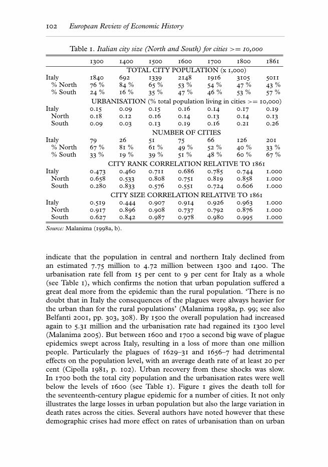
Table 1 reveals large fluctuations in total city population as well as inurbanisation rates between 1300 and 1861. Between the North and the Southwe find clear differences in long-term urban development. The North startsout in 1300 as having a much more developed urban system than the South,with a larger urban population and a higher urbanisation rate. However,during our sample period the South slowly overtakes the North both interms of total urban population as well as in urbanisation rate (the Northeven becomes slightly less urbanised over the centuries).
As to the major shocks that hit the Italian cities during our sampleperiod the plague epidemics clearly stand out. The death toll of the BlackDeath between 1348 and 1351 is estimated at about 40 per cent of thetotal population of the peninsula. Recent calculations by Malanima (2005)
102 European Review of Economic History
Table 1. Italian city size (North and South) for cities >= 10,000
1300 1400 1500 1600 1700 1800 1861
TOTAL CITY POPULATION (x 1,000)Italy 1840 692 1339 2148 1916 3105 5011
% North 76 % 84 % 65 % 53 % 54 % 47 % 43 %% South 24 % 16 % 35 % 47 % 46 % 53 % 57 %
URBANISATION (% total population living in cities >= 10,000)Italy 0.15 0.09 0.15 0.16 0.14 0.17 0.19
North 0.18 0.12 0.16 0.14 0.13 0.14 0.13South 0.09 0.03 0.13 0.19 0.16 0.21 0.26
NUMBER OF CITIESItaly 79 26 51 75 66 126 201
% North 67 % 81 % 61 % 49 % 52 % 40 % 33 %% South 33 % 19 % 39 % 51 % 48 % 60 % 67 %
CITY RANK CORRELATION RELATIVE TO 1861Italy 0.473 0.460 0.711 0.686 0.785 0.744 1.000
North 0.658 0.533 0.808 0.751 0.819 0.858 1.000South 0.280 0.833 0.576 0.551 0.724 0.606 1.000
CITY SIZE CORRELATION RELATIVE TO 1861Italy 0.519 0.444 0.907 0.914 0.926 0.963 1.000
North 0.917 0.896 0.908 0.737 0.792 0.876 1.000South 0.627 0.842 0.987 0.978 0.980 0.995 1.000
Source: Malanima (1998a, b).
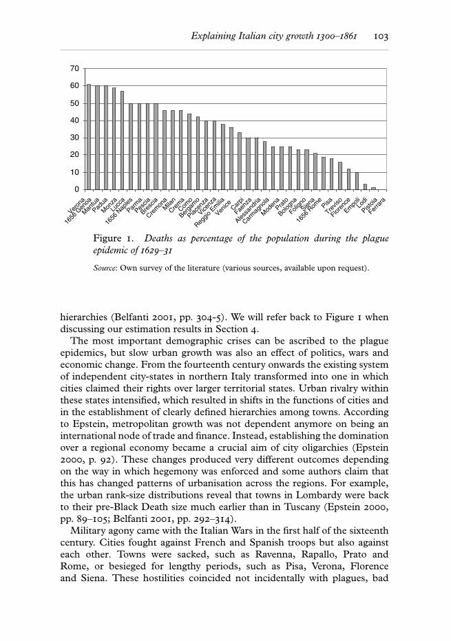
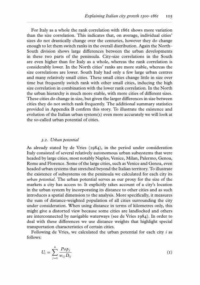
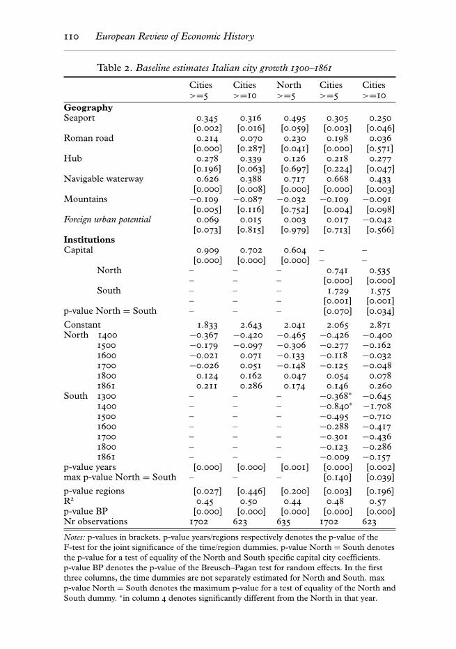
indicate that the population in central and northern Italy declined froman estimated 7.75 million to 4.72 million between 1300 and 1400. Theurbanisation rate fell from 15 per cent to 9 per cent for Italy as a whole(see Table 1), which confirms the notion that urban population suffered agreat deal more from the epidemic than the rural population. ‘There is nodoubt that in Italy the consequences of the plagues were always heavier forthe urban than for the rural populations’ (Malanima 1998a, p. 99; see alsoBelfanti 2001, pp. 303, 308). By 1500 the overall population had increasedagain to 5.31 million and the urbanisation rate had regained its 1300 level(Malanima 2005). But between 1600 and 1700 a second big wave of plagueepidemics swept across Italy, resulting in a loss of more than one millionpeople. Particularly the plagues of 1629–31 and 1656–7 had detrimentaleffects on the population level, with an average death rate of at least 20 percent (Cipolla 1981, p. 102). Urban recovery from these shocks was slow.In 1700 both the total city population and the urbanisation rates were wellbelow the levels of 1600 (see Table 1). Figure 1 gives the death toll forthe seventeenth-century plague epidemic for a number of cities. It not onlyillustrates the large losses in urban population but also the large variation indeath rates across the cities. Several authors have noted however that thesedemographic crises had more effect on rates of urbanisation than on urban
Explaining Italian city growth 1300–1861 103
0
10
20
30
40
50
60
70
Veron
a
1656
Gen
oa
Man
tua
Padua
Mon
za
Lucc
a
1656
Nap
les
Parm
a
Pescia
Bresc
ia
Crem
onaM
ilan
Crem
a
Como
Berga
mo
Piacen
za
Vicenz
a
Reggio
Em
ilia
Venice Car
pi
Faenz
a
Alessa
ndria
Carm
agno
la
Mod
enaPra
to
Bologn
a
Folign
oSien
a
1656
Rom
ePisa
Trevis
o
Floren
ce
Empo
liLo
di
Pistoia
Ferra
ra
Figure 1. Deaths as percentage of the population during the plagueepidemic of 1629–31
Source: Own survey of the literature (various sources, available upon request).
hierarchies (Belfanti 2001, pp. 304-5). We will refer back to Figure 1 whendiscussing our estimation results in Section 4.
The most important demographic crises can be ascribed to the plagueepidemics, but slow urban growth was also an effect of politics, wars andeconomic change. From the fourteenth century onwards the existing systemof independent city-states in northern Italy transformed into one in whichcities claimed their rights over larger territorial states. Urban rivalry withinthese states intensified, which resulted in shifts in the functions of cities andin the establishment of clearly defined hierarchies among towns. Accordingto Epstein, metropolitan growth was not dependent anymore on being aninternational node of trade and finance. Instead, establishing the dominationover a regional economy became a crucial aim of city oligarchies (Epstein2000, p. 92). These changes produced very different outcomes dependingon the way in which hegemony was enforced and some authors claim thatthis has changed patterns of urbanisation across the regions. For example,the urban rank-size distributions reveal that towns in Lombardy were backto their pre-Black Death size much earlier than in Tuscany (Epstein 2000,pp. 89–105; Belfanti 2001, pp. 292–314).
Military agony came with the Italian Wars in the first half of the sixteenthcentury. Cities fought against French and Spanish troops but also againsteach other. Towns were sacked, such as Ravenna, Rapallo, Prato andRome, or besieged for lengthy periods, such as Pisa, Verona, Florenceand Siena. These hostilities coincided not incidentally with plagues, bad
104 European Review of Economic History
harvests and famines. Initially most cities were able to recover from theresulting demographical shocks. Halfway through the sixteenth centurynorthern Italy was still the largest industrial area in Europe. A definitivereversal of fortune came with the severe food crises 50 years later in the1590s.
Recent analyses, however, paint a subtler picture, i.e. one characterisedby only relative economic decline, due to the loss of economic primacy inEurope and to shifts in economic activity between town and countryside.8
According to this approach structural forces and shifting patterns of trade arestressed. For example, Venetian leadership in the Mediterranean economywitnessed a downturn when it lost its spice trade to the Atlantic ports.The loss of the northern markets for textiles and luxuries coincided withsupply-side problems in urban areas. Italian cities lost their competitiveedge to northwestern Europe (Broadberry and Gupta 2006, p. 10). Highproduction costs and high urban taxation rates together with monopolisticpractices of guilds moved industrial producers to smaller cities and to thecountryside (e.g. textile production and raw silk production), where wagesand rates of taxation were lower. Despite these relative drawbacks, however,Italy remained the country with the largest urban population in Europe(DeLong and Shleifer 1993, p. 678).9
The above-described incidental shocks like the plague, wars or faminesand also the more enduring structural changes in e.g. trade patterns andinstitutional developments can in principle affect the position of individualcities in the total distribution of cities. This makes the general consensus onthe stability of the European urban system(s) alluded to in the introduction(see de Vries 1984 and Hohenberg 2004) indeed quite remarkable, as itwould imply that all these potential effects leave the urban system and alsoindividual cities largely unaffected. To see if the Italian data support thisnotion of stability, the bottom part of Table 1 provides, as a first pass,both the rank and the size correlation of the Italian cities in our data setwith their respective rank and size in 1861. The rank correlations revealthe comparability of the ranking of individual cities in the overall city-size distribution in a particular century with the ranking in 1861. The sizecorrelations lead to similar observations but this time in terms of actualpopulation size. The two statistics complement each other as a change ina city’s size need not result in a change in the city’s rankings and viceversa.
8 For a discussion see Malanima (2006, pp. 108–11).9 If we count the number of cities with more than 10,000 inhabitants, in both 1300 and 1861
Italy was still the leading European country with respectively 79 and 201 cities with morethan 10,000 inhabitants (see Table 1), which was ahead of countries like France andEngland.
Explaining Italian city growth 1300–1861 105
For Italy as a whole the rank correlation with 1861 shows more variationthan the size correlation. This indicates that, on average, individual cities’sizes do not drastically change over the centuries, however they do changeenough to let them switch ranks in the overall distribution. Again the North–South division shows large differences between the urban developmentsin these two parts of the peninsula. City-size correlations in the Southare even higher than for Italy as a whole, whereas the rank correlation isconsiderably lower. In the North cities’ ranks are more stable, whereas thesize correlations are lower. South Italy had only a few large urban centresand many relatively small cities. These small cities change little in size overtime but frequently switch rank with other small cities, inducing the highsize correlation in combination with the lower rank correlation. In the Norththe urban hierarchy is much more stable, with more cities of different sizes.These cities do change in size, but given the larger differences in size betweencities they do not switch rank frequently. The additional summary statisticsprovided in Appendix B confirm this story. To illustrate the existence andevolution of the Italian urban system(s) even more accurately we will look atthe so-called urban potential of cities.
3.2. Urban potential
As already stated by de Vries (1984), in the period under considerationItaly consisted of several relatively autonomous urban subsystems that wereheaded by large cities, most notably Naples, Venice, Milan, Palermo, Genoa,Rome and Florence. Some of the large cities, such as Venice and Genoa, evenheaded urban systems that stretched beyond the Italian territory. To illustratethe existence of subsystems on the peninsula we calculated for each city itsurban potential. The urban potential serves as our proxy for the size of themarkets a city has access to. It explicitly takes account of a city’s locationin the urban system by incorporating its distance to other cities and as suchintroduces a spatial dimension to the analysis. More specifically, it measuresthe sum of distance-weighted population of all cities surrounding the cityunder consideration. When using distance in terms of kilometres only, thismight give a distorted view because some cities are landlocked and othersare interconnected by navigable waterways (see de Vries 1984). In order todeal with these differences we use distance weights that highlight specialtransportation characteristics of certain cities.
Following de Vries, we calculated the urban potential for each city i asfollows:
Ui =n∑
j=1
Pop j
wi j Di j(1)
106 European Review of Economic History
where Popj is the population of city j, Dij is the great-circle distance betweencity i and city j and wij is a distance weight defined as follows:
wi j =
⎧⎪⎪⎪⎪⎪⎪⎪⎪⎨⎪⎪⎪⎪⎪⎪⎪⎪⎩
0.5 if city i and city j both major seaports0.75 if city i and city j connected by a navigable waterway0.8 if city i and city j both located on a Roman road0.95 if city i a major seaport and city j on the coast but no
major seaport0.975 if city i and city j both on the coast but no major seaports1 if none of the above or i = j
(2)
Note that we do not weight own city population when calculating the urbanpotential by taking Dij = 1 if i = j, which is different from de Vries who appliesDij = 20 if i = j. We see no reason to weight own city population, because weargue that own city population constitutes the most relevant accessible poolof potential workers/consumers to a specific city.
Using the calculated urban potential per city we are able to sketch thedevelopment of urban subsystems in Italy over time very accurately. Themaps in Appendix C show contour shades of the urban potential over thecenturies, with the darker (lighter) regions indicating highly (less) urbanisedareas respectively. They show how in the North a pronounced, dense urbansystem existed, with major cities such as Florence, Milan, Venice andBologna surrounded by medium-sized cities like e.g. Siena, Genoa, Cremonaand Brescia. From 1600 onwards, the rapid rise of Turin is clearly visible. Inthe South three large subsystems appear around Rome, Naples and Palermo.In contrast to the North, these systems are heavily concentrated aroundthe main cities with hardly any other medium-sized cities in the immediatesurroundings. From 1800, more cities appear, such as the subsystem ofBari.10 A comparison between the maps of 1300 and 1400 clearly reveals thedevastating impact of the bubonic plague around 1350 on the urban systemsin Italy. During the sixteenth century the demographical recovery after theItalian Wars shows up, and this contrasts with the seventeenth century whichsaw new wars and subsequent plague episodes. When comparing 1600 with1700 one can see a decline in the extent of the urban system in the North,whereas e.g. the system around Rome increases in size.
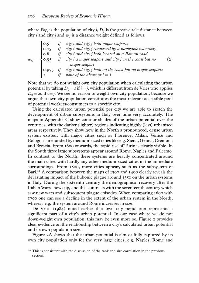
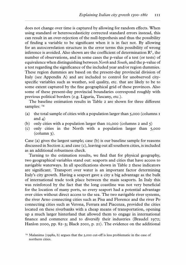
De Vries (1984) noted earlier that own city population represents asignificant part of a city’s urban potential. In our case where we do notdown-weight own population, this may be even more so. Figure 2 providesclear evidence on the relationship between a city’s calculated urban potentialand its own population size.
Figure 2A shows that the urban potential is almost fully captured by itsown city population only for the very large cities, e.g. Naples, Rome and
10 This is consistent with the discussion of the rank and size correlation in the previoussection.
Explaining Italian city growth 1300–1861 107
In u
rban
pot
entia
l
In fo
reig
n po
tent
ial
Figure 2. (A) City population vs urban potential (B) City populationvs foreign potential
Notes: The bold line in each figure is the 45◦-degree line. The correlation betweenurban potential and foreign potential and own city population is 0.69 and 0.06
respectively (the correlation with foreign potential is also not significant even at the10 per cent level, whereas the correlation with urban potential is very significant).
Milan (see also Table C1 in Appendix C). It is only for smaller cities thatthe urban potential clearly exceeds the own city size.11 To abstract fromthe part of urban potential due to own city population, we also calculatethe urban potential excluding the own city size, what we call here the foreignurban potential. It measures the density of the urban system in the areasurrounding a city. Although foreign potential exceeds own city populationonly for the smaller cities, this indicator is not significantly correlated withown city size as shown in Figure 2B. Two large cities in close proximity seemto be the exception; usually the larger city is surrounded by several smallercities.
Table C1 and Figure C1 in Appendix C give additional information on theactual movement of the largest individual cities within the city distribution,supplementing the information given by the rank and size correlation shownin Table 1 and the urban potential maps of Appendix C. It shows that atthe beginning of the sample period the northern Italian cities dominate theirsouthern counterparts in terms of size. From the fifteenth century onwards,however, the southern cities quickly gain importance. In 1800 Naples, Romeand Palermo are the three largest urban centres of the peninsula. Therankings also show that in the North the dynamics of the largest cities interms of their rank are more pronounced. Although the large northern citiesin the years around 1300 are generally also among the largest northerncities in 1861, notable changes in rank take place, in contrast to the muchmore stable South. Florence, for example, was second amongst the northern
11 Note that by construction a city’s urban potential is never smaller than its own population.
108 European Review of Economic History
cities in 1300, but occupied only fifth place in 1500, and ended up as thefourth largest northern city in 1861. At the end of the sample period, Siena,Piacenza, Cremona, Brescia and also Venice are additional examples of citiesmoving down the urban hierarchy in the North. Cities like Genoa and Turintook their place instead. Being one of the smaller cities in the earlier centuries,Turin became a capital city in 1568 and quickly moved upwards in the city-size ranking, ending up as the second largest northern city in 1861.12
Overall the statistics presented in Section 3 lead to the followingobservations. The impact of large shocks (for example, the Black Death inthe fourteenth century, the plagues and the political and economic turmoilin the seventeenth century) is clearly visible in the data and we show thatthe position of individual cities is far from constant through time. Thereis, however, a remarkable degree of continuity in the urban system as awhole, both in the North and the South. Stability amidst change seems tosum up the material presented in this section. This qualification is differentfrom the description by Hohenberg (2004) who found the system of citiesin Europe ‘remarkably stable’. Our conclusion immediately raises a newand more fundamental question. What are the determinants of Italiancity growth between 1300 and 1861 that help to explain the city trendsdiscussed above? The rest of our article aims to provide some answers to thisquestion.
4. The determinants of Italian city growth 1300–1861
4.1. Methodology
As we have data on individual cities over a long period of time, the useof multivariate panel data regression analysis is an obvious choice to lookfor evidence on possible determinants of the development of Italy’s cities.This enables us to distinguish between factors that are constant over timeand those that are not. Our method is as follows. The dependent variable isalways the log of city size. This implies that the coefficients on the includedvariables can be interpreted as relative changes, e.g. the coefficient on ourcapital city dummy indicates how much per cent larger the average capitalcity is relative to the average non-capital city. We use centennial data on thepopulation size of settlements in Italy that had at least 10,000 inhabitantsin the period 1300–1861 as our baseline sample. For completeness we alsopresent estimation results for the 5,000 inhabitants’ cut-off. All estimationresults are obtained using a random effects GLS panel estimator, which
12 When looking at the foreign urban potential rankings instead, one also observes a shiftfrom a top 10 dominated by northern cities at the beginning of the sample period to onedominated by southern cities (mostly those around Rome and Naples) in 1861 (resultsare available upon request).
Explaining Italian city growth 1300–1861 109
allows for unobserved heterogeneity over the cities in our sample that isuncorrelated with the regressors. In all cases the Breusch–Pagan statisticindicates that this specification is preferred over a standard pooled panelregression (see p-value BP in corresponding tables).
We distinguish between three sets of explanatory variables: (i) geographicalvariables; (ii) political/institutional variables and (iii) city-invariant century-specific variables. The last set of variables will be captured either by aset of time (i.e. century) dummies or by a time trend and two dummyvariables capturing the effect of the plague epidemics in the fourteenth andseventeenth centuries respectively.13 We split the first set of explanatoryvariables further into variables related to a city’s physical geography, i.e.being a major seaport, being located at sea, on a navigable river, at morethan 800m above sea level, on a Roman road or a crossroad of two Romanroads, and its relative geography, i.e. a city’s access to markets other than itsown measured by foreign urban potential. As for the second set of variables,the political/institutional variables, we include a capital city dummy in ourbaseline estimations. Being a (regional) capital is expected to contributepositively to city size, since government is able to draw ‘resources from theterritory as a whole to the political and administrative capital, whose regionalhegemony therefore tends to increase’ (Epstein 1993, p. 457; see also Adesand Glaeser 1995). Also, we explicitly allow for differences between theNorth and the South of Italy, and for the fact that these differences mayevolve over time. Finally, when extending the baseline estimates in Section4.3, we will make use of those variables already mentioned in Section 2 asintroduced by Acemoglu et al. (2005), De Long and Shleifer (1993) andTilly (1990) that aim to capture the evolution of institutions in Italy (thelatter two do so by explicitly making a distinction between North and SouthItaly).
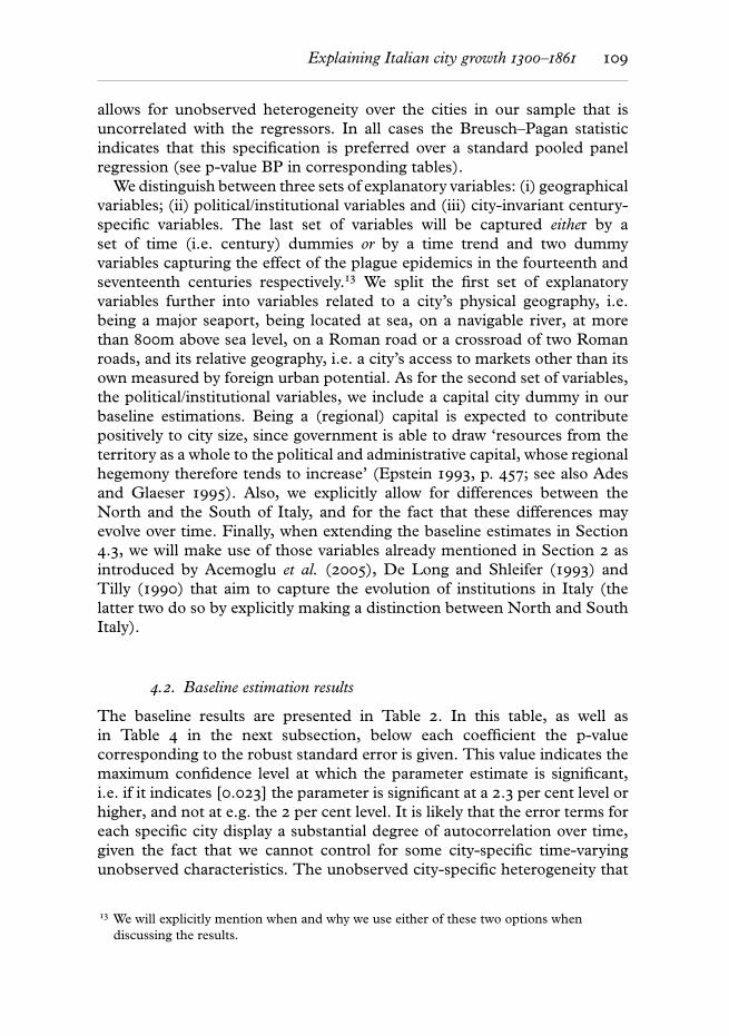
4.2. Baseline estimation results
The baseline results are presented in Table 2. In this table, as well asin Table 4 in the next subsection, below each coefficient the p-valuecorresponding to the robust standard error is given. This value indicates themaximum confidence level at which the parameter estimate is significant,i.e. if it indicates [0.023] the parameter is significant at a 2.3 per cent level orhigher, and not at e.g. the 2 per cent level. It is likely that the error terms foreach specific city display a substantial degree of autocorrelation over time,given the fact that we cannot control for some city-specific time-varyingunobserved characteristics. The unobserved city-specific heterogeneity that
13 We will explicitly mention when and why we use either of these two options whendiscussing the results.
110 European Review of Economic History
Table 2. Baseline estimates Italian city growth 1300–1861
Cities>=5
Cities>=10
North>=5
Cities>=5
Cities>=10
GeographySeaport 0.345 0.316 0.495 0.305 0.250
[0.002] [0.016] [0.059] [0.003] [0.046]Roman road 0.214 0.070 0.230 0.198 0.036
[0.000] [0.287] [0.041] [0.000] [0.571]Hub 0.278 0.339 0.126 0.218 0.277
[0.196] [0.063] [0.697] [0.224] [0.047]Navigable waterway 0.626 0.388 0.717 0.668 0.433
[0.000] [0.008] [0.000] [0.000] [0.003]Mountains −0.109 −0.087 −0.032 −0.109 −0.091
[0.005] [0.116] [0.752] [0.004] [0.098]Foreign urban potential 0.069 0.015 0.003 0.017 −0.042
[0.073] [0.815] [0.979] [0.713] [0.566]InstitutionsCapital 0.909 0.702 0.604 – –
[0.000] [0.000] [0.000] – –North – – – 0.741 0.535
– – – [0.000] [0.000]South – – – 1.729 1.575
– – – [0.001] [0.001]p-value North = South – – – [0.070] [0.034]
Constant 1.833 2.643 2.041 2.065 2.871North 1400 −0.367 −0.420 −0.465 −0.426 −0.400
1500 −0.179 −0.097 −0.306 −0.277 −0.1621600 −0.021 0.071 −0.133 −0.118 −0.0321700 −0.026 0.051 −0.148 −0.125 −0.0481800 0.124 0.162 0.047 0.054 0.0781861 0.211 0.286 0.174 0.146 0.260
South 1300 – – – −0.368∗ −0.6451400 – – – −0.840∗ −1.7081500 – – – −0.495 −0.7101600 – – – −0.288 −0.4171700 – – – −0.301 −0.4361800 – – – −0.123 −0.2861861 – – – −0.009 −0.157
p-value years [0.000] [0.000] [0.001] [0.000] [0.002]max p-value North = South – – – [0.140] [0.039]
p-value regions [0.027] [0.446] [0.200] [0.003] [0.196]R2 0.45 0.50 0.44 0.48 0.57p-value BP [0.000] [0.000] [0.000] [0.000] [0.000]Nr observations 1702 623 635 1702 623
Notes: p-values in brackets. p-value years/regions respectively denotes the p-value of theF-test for the joint significance of the time/region dummies. p-value North = South denotesthe p-value for a test of equality of the North and South specific capital city coefficients.p-value BP denotes the p-value of the Breusch–Pagan test for random effects. In the firstthree columns, the time dummies are not separately estimated for North and South. maxp-value North = South denotes the maximum p-value for a test of equality of the North andSouth dummy. ∗in column 4 denotes significantly different from the North in that year.
Explaining Italian city growth 1300–1861 111
does not change over time is captured by allowing for random effects. Whenusing standard or heteroscedasticity corrected standard errors instead, thiscan result in an over-rejection of the null-hypothesis and thus the possibilityof finding a variable to be significant when it is in fact not. By allowingfor an autocorrelation structure in the error terms this possibility of wronginference is avoided. Also shown are the coefficient of determination R2, thenumber of observations, and in some cases the p-value of a test (or tests) ofequivalence when distinguishing between North and South, and the p-value ofa test regarding the significance of the included year and/or region dummies.These region dummies are based on the present-day provincial division ofItaly (see Appendix A) and are included to control for unobserved city-specific variables such as weather, soil quality, etc. that are likely to be tosome extent captured by the fine geographical grid of these provinces. Alsosome of these present-day provincial boundaries correspond roughly withprevious political borders (e.g. Liguria, Tuscany, etc.).
The baseline estimation results in Table 2 are shown for three differentsamples: 14
(a) the total sample of cities with a population larger than 5,000 (columns 1
and 4)(b) only cities with a population larger than 10,000 (columns 2 and 5)(c) only cities in the North with a population larger than 5,000
(column 3).
Case (a) gives the largest sample; case (b) is our baseline sample for reasonsdiscussed in Section 2; and case (c), leaving out all southern cities, is includedas an additional robustness check.
Turning to the estimation results, we find that for physical geography,two geographical variables stand out: seaports and cities that have access tonavigable waterways. In all specifications shown in Table 2 these indicatorsare significant. Transport over water is an important factor determiningItaly’s city growth. Having a seaport gave a city a big advantage as the bulkof international trade took place between the main seaports. In Italy thiswas reinforced by the fact that the long coastline was not very beneficialfor the location of many ports, so every seaport had a potential advantageover cities without direct access to the sea. The two navigable river systems,the river Arno connecting cities such as Pisa and Florence and the river Poconnecting cities such as Verona, Ferrara and Piacenza, provided the citieslocated on these riverbanks with a cheap means of transportation, openingup a much larger hinterland that allowed them to engage in internationalfinance and commerce and to diversify their industries (Braudel 1972;Hanlon 2000, pp. 82–3; Black 2001, p. 21). The evidence on the additional
14 Malanima (1998a, b) argues that the 5,000 cut-off is less problematic in the case ofnorthern cities.
112 European Review of Economic History
physical geography variables (Roman road, hub, mountains) turns out to besomewhat more mixed. In our baseline sample of cities larger than 10,000,being a hub has a significantly positive effect on a city’s population size inline with predictions from Fujita and Mori (1996). However, in the samplesincluding also the smaller cities (columns 1, 3 and 4) this variable is no longersignificant, which is mainly due to the fact that these samples include somehub cities that are quite small (e.g. Trieste, Rimini, Capua and Brindisi),shedding some doubt on an unequivocal positive effect of being a hub city.Location on a Roman road or in the mountains, on the other hand, doeshave a significantly positive and negative effect respectively when includingthe smaller cities between 5,000 and 10,000 inhabitants, whereas they areboth not significant in our baseline sample. This result is driven by the factthat by adding the smaller cities that are on the one hand more likely to belocated in the mountains and on the other hand less likely to be on a majorRoman road, a part of the difference in population can now be ascribed tothese two variables.15 It indicates that these two variables are very relevantfor the possibility of the smaller cities becoming larger population centres,whereas they lose their importance once a certain level of population isreached (King 1985, p. 145).
So far, the role of geography in determining Italian city size has beenlimited to physical geography. From modern location theories, like the neweconomic geography, we know that it might not be only the physical aspect ofgeography but also the relative aspect of geography that may be of importancefor Italian city growth (Krugman 1991). To this end, we included foreignurban potential from Section 3.2 in the set of regressors as a measure ofa city’s access to other cities’ markets.16 In all five cases urban potentialis not significant.17 The most straightforward way to interpret this is thatgood access to other (large) cities does not significantly contribute to acity’s growth; in the period under consideration the kind of spatial linkagesthat are captured by the urban potential variable were limited in Italy (deVries, 1984). From new economic geography theory we know that whentransportation costs are too high, or production is not yet characterised by
15 40% (28%) of cities with a population between 5,000 and 10,000 inhabitants are locatedin mountains (on a Roman road) compared to 18% (46%) of cities with more than10,000 inhabitants.
16 We chose foreign urban potential because urban potential (which includes own-citypopulation) largely coincides with own-city population (compare Figures 2A and 2B),which immediately raises concerns regarding the endogeneity of this variable. We ran thesame regressions with urban potential instead of foreign urban potential and the resultsare similar in the sense that urban potential is never significant.
17 It is significant at the 10 per cent level when considering all cities larger than 5,000
inhabitants, however, significance is totally lost in this case when allowing for somedifferences between North and South Italy (see column 4). Also when distinguishingbetween North and South or over time, foreign urban potential is never significant(results available upon request).
Explaining Italian city growth 1300–1861 113
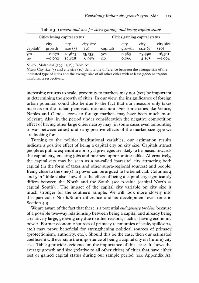
Table 3. Growth and size for cities gaining and losing capital status
Cities losing capital status Cities gaining capital status
capital?citygrowth
citysize (5)
city size(10) capital?
citygrowth
citysize (5)
city size(10)
yes 0.070 24,623 13,135 yes 0.383 29,390 16,501no −0.092 17,828 6,989 no 0.066 4,165 −5,904
Source: Malanima (1998 a, b); Table A1.Notes: City size (5) and city size (10) denote the difference between the average size of theindicated type of cities and the average size of all other cities with at least 5,000 or 10,000
inhabitants respectively.
increasing returns to scale, proximity to markets may not (yet) be importantin determining the growth of cities. In our view, the insignificance of foreignurban potential could also be due to the fact that our measure only takesmarkets on the Italian peninsula into account. For some cities like Venice,Naples and Genoa access to foreign markets may have been much morerelevant. Also, in the period under consideration the negative competitioneffect of having other large cities nearby may (in some cases even amountingto war between cities) undo any positive effects of the market size type weare looking for.
Turning to the political/institutional variables, our estimation resultsindicate a positive effect of being a capital city on city size. Capitals attractpeople as public expenditure or royal privileges are likely to be biased towardsthe capital city, creating jobs and business opportunities alike. Alternatively,the capital city may be seen as a so-called ‘parasite’ city attracting bothcapital (in the form of taxes and other supra-regional sources) and people.Being close to the one(s) in power can be argued to be beneficial. Columns 4
and 5 in Table 2 also show that the effect of being a capital city significantlydiffers between the North and the South (see p-value (capital North =capital South)). The impact of the capital city variable on city size ismuch stronger for the southern sample. We will look more closely intothis particular North/South difference and its development over time inSection 4.3.
We are aware of the fact that there is a potential endogeneity problem becauseof a possible two-way relationship between being a capital and already beinga relatively large, growing city due to other reasons, such as having economicpower. Former economic sources of primacy (economies of scale, spillovers,etc.) may prove beneficial for strengthening political sources of primacy(protectionism, authority, etc.). Should this be the case, then our estimatedcoefficient will overstate the importance of being a capital city on (future) citysize. Table 3 provides evidence on the importance of this issue. It shows theaverage growth and size (relative to all other cities) of cities that have eitherlost or gained capital status during our sample period (see Appendix A),
114 European Review of Economic History
distinguishing explicitly between the periods during which these cities didand did not enjoy capital status respectively.
The results in Table 3 clearly show that cities both losing and gainingcapital status are growing fastest when they are a capital. Population growthincreases (declines) rapidly in the period after gaining (losing) capital status.This is subsequently reflected in a higher than average city size when beinga capital. There is no evidence that cities were already in a period of declinebefore losing their capital status, their population during that period beingmuch larger than the average city (both compared to all other cities largerthan 5,000 and larger than 10,000 inhabitants respectively). As for theargument that larger cities are the ones gaining capital status, this doesnot seem to be true either. Cities gaining capital status were on averagesomewhat smaller compared to other cities with at least 10,000 inhabitants.These results lead us to conclude that we can be confident that we haveidentified a causal effect of being a capital city on subsequent populationgrowth.
There is thus no clear-cut evidence that there is a one-to-one relationshipbetween having economic power first and then getting political power asa result. Not all large economic centres were to become capitals later.This depended very much on the strength of the territorial state the citybelonged to and on the degree of political coordination (Epstein 2000,p. 95). Turin may serve as an example. Its rise to dominance in Piedmontwas the result of the strictly political project to turn the city into the centreof a strongly centralised state, and subsequent mercantilist policies made italso the economic centre (Belfanti 2000, pp. 299–300). Similarly, Naplesestablished its lead after 1450 through a series of privileges granted by theAragonese sovereigns, including the full exemption of residents from directtaxation, which was later confirmed by the Spanish monarchy (Marin 2000,p. 321). As a final example we mention Palermo. This town together withMessina dominated the island of Sicily during the thirteenth century, lost itsprimacy in the fourteenth century, then became the official capital duringthe Catalan–Aragonese monarchy. However, it could only increase its leadover its peers after 1600.
Returning to our baseline estimation results, the bottom half of Table 2
finally shows the estimated century-specific dummies. These dummiescapture how the average city size changes over time. As can be seen, centuryeffects are always highly significant. When also allowing these century effectsto differ between North and South Italy, they are found to be significantlydifferent in the case of our baseline sample. Instead of merely includingthese time dummies to control for the evolution in average city size between1300 and 1861, the next subsection tries to find an explanation by relatingthe observed evolution of these century-specific effects and its differencebetween North and South to the institutional development of the two partsof the peninsula.
Explaining Italian city growth 1300–1861 115
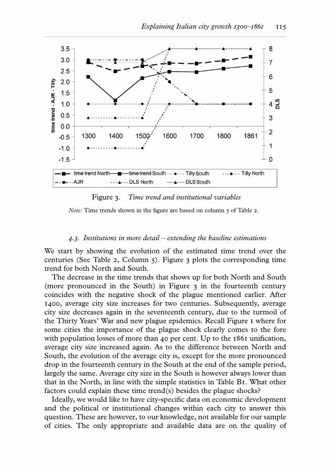
Figure 3. Time trend and institutional variables
Note: Time trends shown in the figure are based on column 5 of Table 2.
4.3. Institutions in more detail – extending the baseline estimations
We start by showing the evolution of the estimated time trend over thecenturies (See Table 2, Column 5). Figure 3 plots the corresponding timetrend for both North and South.
The decrease in the time trends that shows up for both North and South(more pronounced in the South) in Figure 3 in the fourteenth centurycoincides with the negative shock of the plague mentioned earlier. After1400, average city size increases for two centuries. Subsequently, averagecity size decreases again in the seventeenth century, due to the turmoil ofthe Thirty Years’ War and new plague epidemics. Recall Figure 1 where forsome cities the importance of the plague shock clearly comes to the forewith population losses of more than 40 per cent. Up to the 1861 unification,average city size increased again. As to the difference between North andSouth, the evolution of the average city is, except for the more pronounceddrop in the fourteenth century in the South at the end of the sample period,largely the same. Average city size in the South is however always lower thanthat in the North, in line with the simple statistics in Table B1. What otherfactors could explain these time trend(s) besides the plague shocks?
Ideally, we would like to have city-specific data on economic developmentand the political or institutional changes within each city to answer thisquestion. These are however, to our knowledge, not available for our sampleof cities. The only appropriate and available data are on the quality of
116 European Review of Economic History
institutions. These data are time-variant but city-invariant. More specifically,we use indices on the evolution of the quality of institutions from threedifferent sources.18 From Acemoglu et al. (2005) we use the ‘protection forcapital index’, which measures the extent to which the political institutionsthat are in place limit the arbitrary use of power by the ruler. The index rangesfrom +1 (there is no effective protection against arbitrary confiscation by theruler) to +7 (the government is formed by and largely influenced/controlledby merchants and middle classes). From Tilly (1990), we use the indexmeasuring the relative development of coercion on the part of the rulerversus the strength of the merchant class (capital). The index distinguishesexplicitly between the North and the South and ranges from –1 (capitaloutruns coercion) to +1 (coercion outruns capital). Finally, from DeLongand Shleifer (1993) we collected a classification of western European regimes.Their index distinguishes explicitly between North and South Italy and takeson values between +1 (there is a full constitutional monarchy or republicin place) to +8 (the political system is characterised by full bureaucraticabsolutism or by rule of military conquerors). Figure 3 plots each of thesethree institutional variables together with the estimated time trends in averagecity size. It shows clearly that all three political-institutional indices suggestthat after 1500 a movement in the direction of absolutist regimes tookplace. The two political regime variables that distinguish between the Northand the South show that this change was much more pronounced in theNorth.
The important shift in the political-institutional structure in the Northas illustrated by Figure 3 is connected to the shift from independent city-states to territorial states. The alleged switch from city-state-based rule bymerchant oligarchies to the assertion of Habsburg authority over northernItaly after 1500 is mentioned as the cause of declining urbanisation and theshift of gravity of the European economy to the north of the Alps (DeLongand Shleifer 1993, p. 677). In the South this change is much less pronounced;Tilly’s less finely graded index does not indicate a switch at all. Throughoutour sample period, the South consists of the Kingdoms of Naples and Sicilyand a large part of the Papal States. Both are examples of absolutist statescentred around their respective capital cities. The observed change after 1500
18 In an earlier version of our article (see Bosker et al. 2007, figure 3 for the correspondingresults), we also looked at the relevance of a number of city-invariant, time-invarianteconomic variables. However, we decided to focus on the political-institutionaldevelopment here, as these economic variables, e.g. agricultural labour productivity andprices of agricultural and non-agricultural goods (as rightly pointed out by twoanonymous referees), are collected for Tuscany and Lombardy only (see Federico andMalanima 2004), which makes it at least doubtful to use them for Italy as a whole. Inaddition, the interpretation of the impact of these economic variables on Italian cities isfar from clear-cut.
Explaining Italian city growth 1300–1861 117
in the DeLong and Shleifer index coincides with the South of Italy comingunder the control of absolutist rule, most notably the Spanish monarchy.
What are the expected effects of the strengthening of the ‘princely’ ruleon city size? And more importantly, can we find empirical evidence thatexplains the observed evolution of Italian cities over time? The first effect ofthe formation of largely absolutist states that can be expected is an increase inthe redirection of resources from both the countryside and other cities to thecapital city, due to an increased ability of the government to enforce centralrule. Especially for the northern Italian urban system this was a novelty:‘Perhaps the most striking effect of state formation on urban structures wasthe invention during the later Middle Ages of the capital city as the politicaland administrative heart of the state’ (Epstein 2000, p. 89). The reasonswhy capital cities might be larger are well documented by Ades and Glaeser(1995). They argue that in more absolutist regimes, capital cities are muchmore successful in relocating wealth from other cities and the countrysideto the capital city through extraction of large rents and taxes; capital citiesact like ‘parasite’ cities. The second effect of such a change is a detrimentaleffect on the population size of the non-capital cities. DeLong and Shleifer(1993) hypothesise that in absolutist states compared to non-absolutist or freestates, urbanisation ratios will be lower, but capital cities will be relativelylarge. They explicitly mention the Kingdom of Naples as a prime examplein favour of their hypothesis. Trade diversion via Naples and resultingeconomic constraints for others cities is only half of the story, however.Recent analyses have shown that the low number of towns of intermediatesize was as much the result of Spanish rule on the one hand and the politicaldominance of Naples on the other. Many towns had been punished bythe monarchy for their pro-French role in the Italian Wars, which deprivedthem of important economic privileges. Spanish rule was generally hostile tolocal autonomy and southern towns could not dominate their hinterlands,as was the case in the North after the Black Death (Marin 2001, p. 322).As a result, Naples did not meet serious competition from nearby or distantneighbours.
To see if we can find systematic evidence in favour of these two hypotheses,we look at each of them separately. First, we would expect the ‘capital citybonus’ to become larger over time, given Italy’s institutional development(see Figure 3). Second, we expect a perverse effect on other, non-capital,cities that suffer more from the parasitic nature of the capital city underabsolutist regimes. Also we postulate that those cities located close to thecapital are potentially affected differently than cities at a larger distancefrom the capital city. In principle, being located close to a capital cityshould not affect the development of cities in its immediate surroundingsnegatively. It could even have a positive effect, as the capital city constitutesan attractive, large market from which cities at close range can reap thebenefits through, for example, trade but also military protection. However
118 European Review of Economic History
under more absolutist regimes the predatory nature of the capital city mayoffset this positive effect by the extraction of rents and imposed taxes.
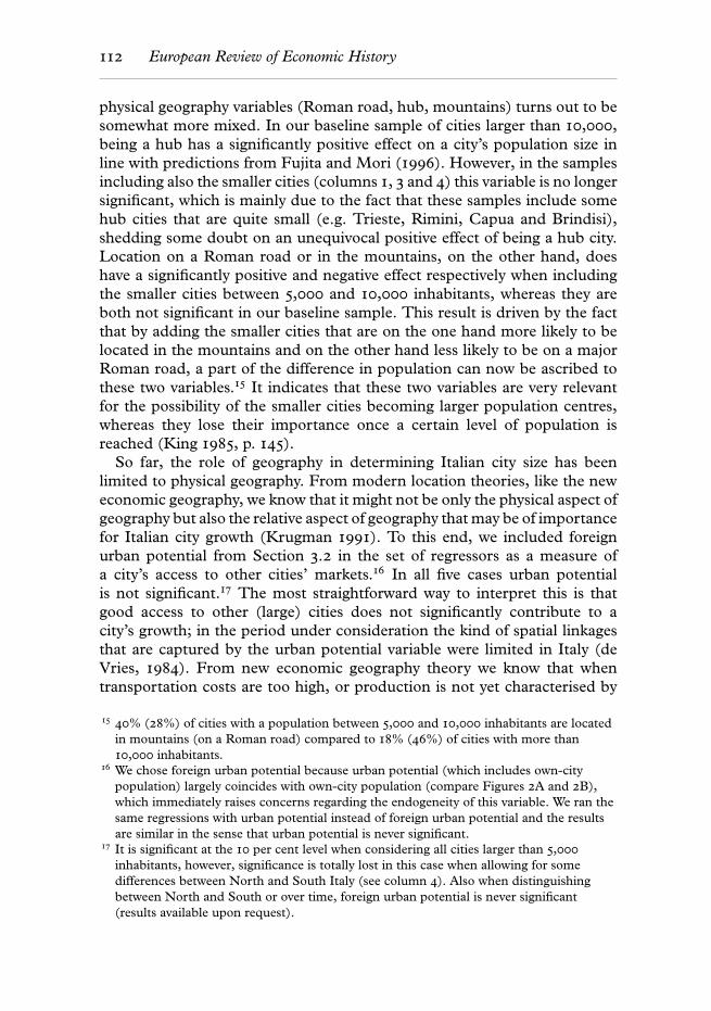
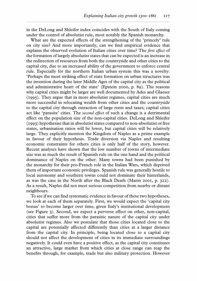
To check the first hypothesis we first of all focus explicitly on the evolutionof capital cities over time and then relate their evolution to our collectedmeasures of institutional quality. The first two columns in Table 4 presentthe estimation results.19 The first column extends the baseline estimates bynot only allowing the capital city bonus to be different between North andSouth, but also to be century-specific. This allows us to track the evolutionof the capital city bonus over time. The result is best illustrated in Figure 4,which plots the estimated century- and North–South-specific coefficients onthe capital city dummy.
Turning to Table 4, note first of all (see p-value capitals) that it is justifiedto include the various capital dummies. Invariably, being a capital city isbeneficial for city size but the ‘capital bonus’ is larger in the South, as isillustrated by the two different axes in Figure 4. According to DeLong andShleifer (1993), southern Italy can be seen as an example of an absolutiststate throughout our sample period. This would help explain why the ‘capitalbonus’ is larger in the South with the Kingdom of Naples and the PapalStates. As to the evolution of the capital city bonus over time, for southerncities the relevance of being a capital city increases markedly over timeafter 1400, corresponding to the rise to dominance most notably of Romeand Naples as the capital cities of the Papal States and the Kingdom ofNaples respectively. The North shows a very different evolution over time,being fairly constant until about 1600; thereafter it starts to increase slightly,taking off only in the 1800s. Apparently the transformation from city-states toterritorial states, and later on to Habsburg rule, had a much less pronouncedeffect.
The results in the second column of Table 4 corroborate this finding.Here we do not estimate the capital city bonus over time, but instead relateits increases to the change in absolutist rule as measured by the DeLongand Shleifer (1993) index (DLS from now on).20 Note that we also replacedthe century dummies by a linear time trend and two ‘plague’ dummies, asit is impossible to use the DLS variable together with century dummies,because this would result in perfect multicollinearity.21 The results can be
19 We will focus on the political/institutional variables in this section. The results on theother included geography variables are always the same as in the baseline resultsdiscussed earlier in Table 2.
20 Results are similar when using either the Acemoglu et al. (2005) or Tilly (1990) variable.We show the results using the DeLong and Shleifer (1993) data as their indexdistinguishes explicitly between the North and the South of Italy as well as beingtime-varying for both parts of the peninsula.
21 The plague dummies are both negative and significant; also we find that the Black Deathin the fourteenth century affected the average city to a much larger extent than theplagues of the seventeenth century.
Explaining
Italiancity
growth
1300–
1861119
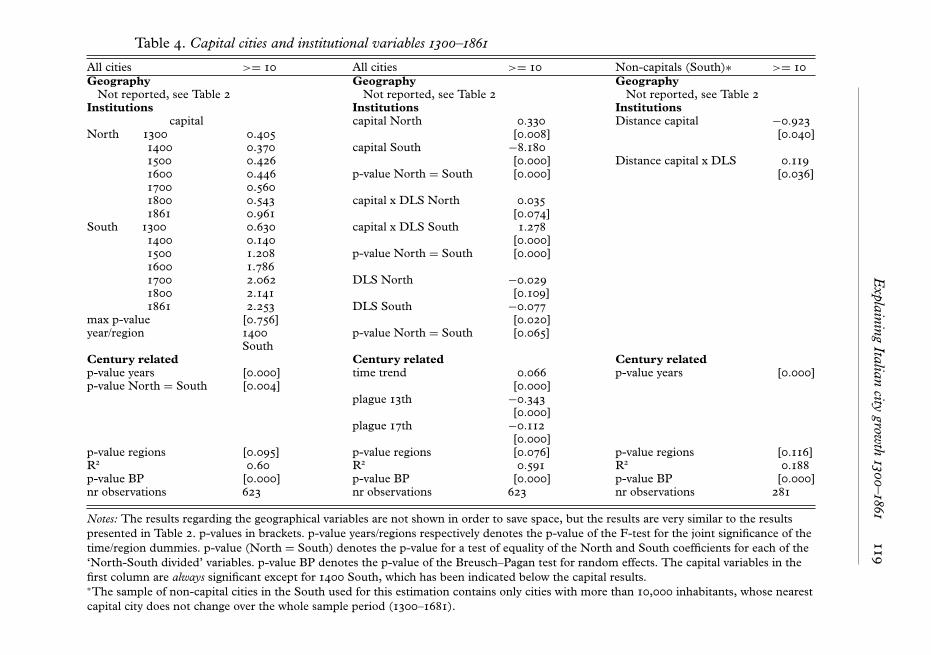
Table 4. Capital cities and institutional variables 1300–1861
All cities >= 10 All cities >= 10 Non-capitals (South)∗ >= 10Geography Geography Geography
Not reported, see Table 2 Not reported, see Table 2 Not reported, see Table 2Institutions Institutions Institutions
capital capital North 0.330 Distance capital −0.923North 1300 0.405 [0.008] [0.040]
1400 0.370 capital South −8.1801500 0.426 [0.000] Distance capital x DLS 0.1191600 0.446 p-value North = South [0.000] [0.036]1700 0.5601800 0.543 capital x DLS North 0.0351861 0.961 [0.074]
South 1300 0.630 capital x DLS South 1.2781400 0.140 [0.000]1500 1.208 p-value North = South [0.000]1600 1.7861700 2.062 DLS North −0.0291800 2.141 [0.109]1861 2.253 DLS South −0.077
max p-value [0.756] [0.020]year/region 1400
Southp-value North = South [0.065]
Century related Century related Century relatedp-value years [0.000] time trend 0.066 p-value years [0.000]p-value North = South [0.004] [0.000]
plague 13th −0.343[0.000]
plague 17th −0.112[0.000]
p-value regions [0.095] p-value regions [0.076] p-value regions [0.116]R2 0.60 R2 0.591 R2 0.188p-value BP [0.000] p-value BP [0.000] p-value BP [0.000]nr observations 623 nr observations 623 nr observations 281
Notes: The results regarding the geographical variables are not shown in order to save space, but the results are very similar to the resultspresented in Table 2. p-values in brackets. p-value years/regions respectively denotes the p-value of the F-test for the joint significance of thetime/region dummies. p-value (North = South) denotes the p-value for a test of equality of the North and South coefficients for each of the‘North-South divided’ variables. p-value BP denotes the p-value of the Breusch–Pagan test for random effects. The capital variables in thefirst column are always significant except for 1400 South, which has been indicated below the capital results.∗The sample of non-capital cities in the South used for this estimation contains only cities with more than 10,000 inhabitants, whose nearestcapital city does not change over the whole sample period (1300–1681).
120 European Review of Economic History
Figure 4. Capital city bonus over time (in North and South)
Notes: Results shown in the figure are based on column 1 of Table 4.
interpreted as follows. The total effect of being a capital city is in this casenot just the estimated coefficient of the capital city dummy. We have toadd to this the estimated coefficient on the ‘capital city x DLS’ variablemultiplied by the actual value of the DLS variable (as shown for both theNorth and the South in Figure 3). So, in the baseline sample of citieslarger than 10,000 inhabitants, the capital city bonus in the period up to1500 is estimated at −8.180 + (7 × 1.278) = 0.766 for the southern capitalcities and 0.330 + (3 × 0.035) = 0.435 for their northern counterparts. From1600 onwards these ‘bonuses’ increase to −8.180 + (8 × 1.278) = 2.044 in theSouth and to 0.330 + (8 × 0.035) = 0.6 in the North. Moreover, the estimatedcoefficient on the ‘capital x DLS’ variable by itself can be interpreted as theeffect on the capital city bonus when moving up on the DLS scale of thedegree of absolutism of the state. The results clearly indicate that first, capitalcities are indeed larger in more absolutist regimes and second, that this effectwas much stronger in the South, clearly corroborating the estimates of thecentury-specific capital city bonus (see Figure 4).
Next we turn to the effect on the non-capital cities. In the second columnof Table 4 the estimated coefficient on the ‘DLS variable’ shows the effectof an increase in the degree of absolutism on non-capital cities. The sign isnegative for both the North and the South, confirming our hypothesis thatnon-capital cities are smaller under more absolutist regimes. These citiessuffer from the parasitical nature of the capital city; they also experiencethe detrimental effect on the incentives for the merchant class to engage in
Explaining Italian city growth 1300–1861 121
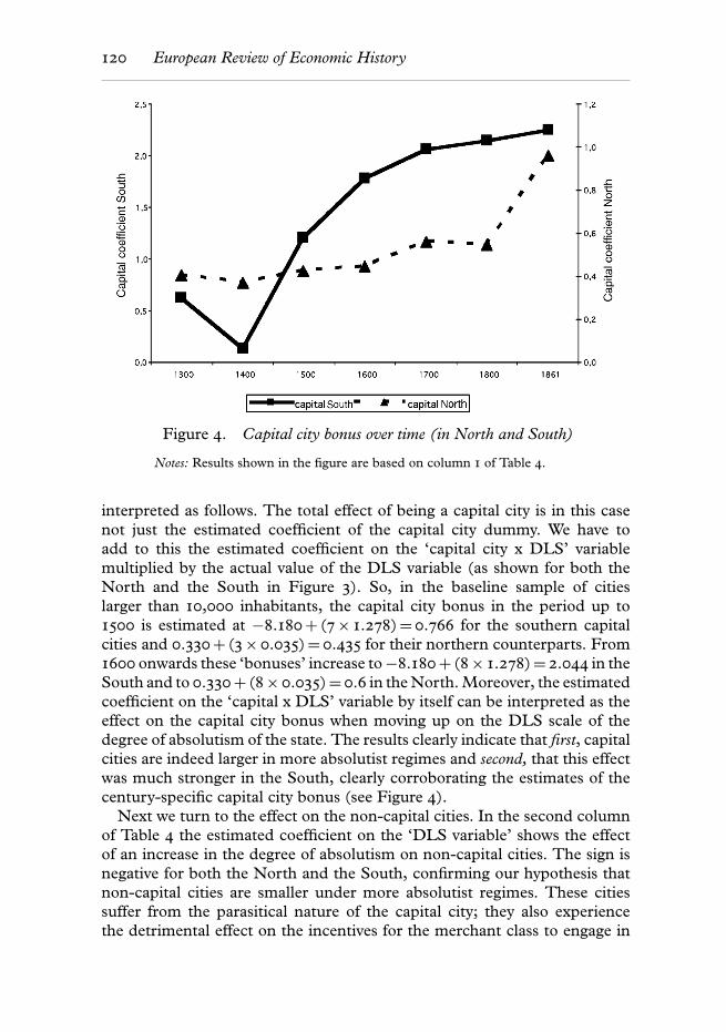
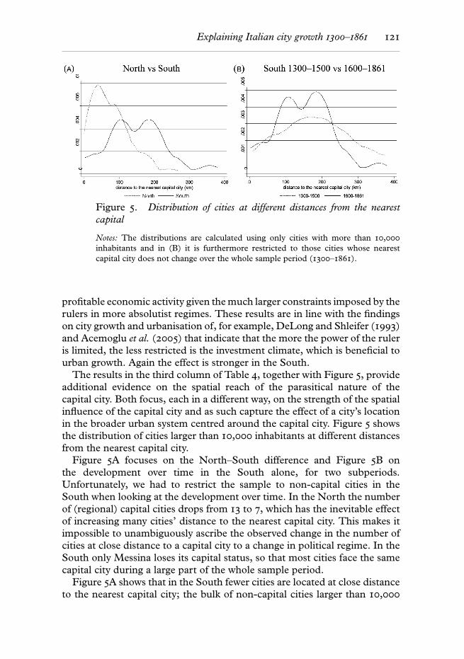
Figure 5. Distribution of cities at different distances from the nearestcapital
Notes: The distributions are calculated using only cities with more than 10,000
inhabitants and in (B) it is furthermore restricted to those cities whose nearestcapital city does not change over the whole sample period (1300–1861).
profitable economic activity given the much larger constraints imposed by therulers in more absolutist regimes. These results are in line with the findingson city growth and urbanisation of, for example, DeLong and Shleifer (1993)and Acemoglu et al. (2005) that indicate that the more the power of the ruleris limited, the less restricted is the investment climate, which is beneficial tourban growth. Again the effect is stronger in the South.
The results in the third column of Table 4, together with Figure 5, provideadditional evidence on the spatial reach of the parasitical nature of thecapital city. Both focus, each in a different way, on the strength of the spatialinfluence of the capital city and as such capture the effect of a city’s locationin the broader urban system centred around the capital city. Figure 5 showsthe distribution of cities larger than 10,000 inhabitants at different distancesfrom the nearest capital city.
Figure 5A focuses on the North–South difference and Figure 5B onthe development over time in the South alone, for two subperiods.Unfortunately, we had to restrict the sample to non-capital cities in theSouth when looking at the development over time. In the North the numberof (regional) capital cities drops from 13 to 7, which has the inevitable effectof increasing many cities’ distance to the nearest capital city. This makes itimpossible to unambiguously ascribe the observed change in the number ofcities at close distance to a capital city to a change in political regime. In theSouth only Messina loses its capital status, so that most cities face the samecapital city during a large part of the whole sample period.
Figure 5A shows that in the South fewer cities are located at close distanceto the nearest capital city; the bulk of non-capital cities larger than 10,000
122 European Review of Economic History
inhabitants are located more than 100 km away from a capital city. In theNorth this is different, with many more cities located close to the nearestcapital city. When making a distinction between the period before and after1500, when the change in political regime was most clear, we observe thatin the South the density of cities at close range to a capital city declinesslightly in the second period, whereas we observe a substantial increase incities between 90 and 200 km from the capital city. These are mainly citieslocated around Bari, as is shown in the urban potential maps in Figure C1.Overall these results strengthen the notion of a parasitical capital city thatdoes not ‘tolerate’ the development of other large cities in its vicinity.
The results in the third column of Table 4 provide complementaryevidence to this. Instead of focusing on the existence of cities larger than10,000 inhabitants (as in Figure 5), we provide results that show the impactof being close to the capital city on a city’s population size (given that a cityis larger than 10,000 inhabitants). To do so, we include the distance tothe nearest capital city as an additional explanatory variable to the baselineregression, both by itself and interacted with the DLS variable to see if we canobserve a change in the effect in the period after 1500 as a result of the changein political regime. The results show that in principle being located close toa capital city in the South positively affects city size. However, this positiveeffect is reduced as the absolutist grip is strengthened, which is shown bythe significantly positive coefficient on the interaction term. When using theactual values of the DLS variable in the South (again see Figure 3), we seethat in the period 1300–1500, distance to the capital city negatively affectscity size (−0.923 + (7 × 0.119) = −0.090), whereas in the period thereafterthis turns into a positive effect (−0.923 + (8 × 0.119) = 0.029). This indicatesthat the institutional change that went along with the imposition of Spanishrule in the South not only affected non-capital city growth negatively (seethe second column of Table 4), but also that cities at closer range to thecapital city suffered more from this than cities at a greater distance.
When we combine all the empirical evidence provided in this subsection,we conclude that a movement away from governments whose arbitrary use ofpower is limited negatively affects the growth of the average city, confirmingthe evidence provided in Acemoglu et al. (2005) and DeLong and Shleifer(1993). Moreover we show that the increase in the degree of absolutism doesnot affect all cities negatively: capital cities benefit from such a development.The difference in the capital city bonus between North and South as wellas its evolution over time confirms the notion of the ‘parasitical nature’of the capital city, relocating wealth from other cities and the countrysideto the capital city through extraction of large rents and taxes (Ades andGlaeser 1995). For the South, this is further confirmed by looking at theevolution over time of the number of cities with at least 10,000 inhabitantslocated at close range to the capital city. Moreover, the evidence on theeffect of distance to the capital city on the average size of those cities that
Explaining Italian city growth 1300–1861 123
are relatively close to the capital city seems to indicate that those cities thatare closer to the capital city are generally larger than those further removedfrom the capital, although this positive effect weakens substantially with anincrease in absolutist rule.
We are aware of the fact that the nature of the North–South difference incity growth that we found may be artificial. The reason why we always finda weaker effect in the North on the capital city bonus and on non-capitalcities is to a large extent due to the absolutist/non-absolutist classificationwe applied. This measure is probably too rough to precisely capture thepolitical and economic reality of northern Italy with its change from freerepublics to princely rule and imperial domination. First, absolutism nevergot hold of the region fully. For example, even after the rise of Spanishdomination in Lombardy the internal organisation of the state remainedpolycentric and was characterised by pluralism (Belfanti 2001, p. 307). Themulti-polar structure of the North, with a less articulated urban hierarchyand spatial specialisation, was in a sense the fruit of long-term politicalfragmentation. Second, although after 1500 the urban hierarchy becamemore pronounced through political and institutional forces, it certainly didnot result in identical patterns of urbanisation and urban growth across thevarious territories. Epstein has shown convincingly that, for example, inthe case of Lombardy the urban economies profited from a clear regionalleader that took up the role of central coordinator (Milan). In contrast, inTuscany the defence of urban vested interests by a narrow-minded Florentineoligarchy was not only detrimental for the economy of the town itself butalso for the surrounding cities (Epstein 2000, pp. 95–6). Thus, as far asthere were ‘absolutist’ tendencies replacing the economic hegemony of thecity-states, it had the effect of either weakening central vested interests or ofstrengthening institutional privileges of a core city. Both outcomes, however,had as a result the displacement of merchants and artisans to the countrysideinstead of to one or two large cities. This could to some extent explain thesmaller capital city bonus and the smaller negative effect on the non-capitalcities that we find for the North compared to the South.
5. Conclusions
In this article we study the evolution of a large sample of Italian cities forthe period 1300–1861. We use various descriptive statistics on individual citysizes and urban potential indicators to highlight the main characteristics ofItaly’s urban system. The southern parts of Italy experienced a relativelymore pronounced change in the city-size distributions over time, with a fewcities, i.e. Rome, Naples and Palermo, gaining dominance from 1400 onand exceeding their northern counterparts in terms of population size. Thecity-size distribution of the northern part of Italy is relatively more stable
124 European Review of Economic History
compared to the southern part, although zooming in on the actual rankingsof cities over the centuries reveals more dynamic movements than one wouldsee by only looking at aggregate statistics. The overall picture we find seemsto be best characterised by ‘stability amidst change’.
Our second contribution is that we go beyond merely describing theevolution of the Italian urban system(s) and explicitly look for importantdeterminants that are behind this observed stability. Our centennialdata allow for panel estimation where city size is regressed on variousgeographical, political and other determinants of city size for the period1300–1861. Using an existing data set from Malanima (1998a, b, 2005), weperform panel estimations where the development of city size and urbanpatterns can be explained by various geographical, institutional and otherdeterminants of city size for the period under consideration. Although largeshocks such as the plague epidemics are clearly visible in the data, ourbaseline estimation results show that the main determinants of Italian citygrowth are physical geography and the predominance of capital cities. Withrespect to geography, being a seaport or having access to navigable waterwaysincreases city size whereas a city’s relative location, as measured by urbanpotential, is not significant. Being a capital city also increases city size. Theestimation results also reveal strong century-specific effects on city growthand these effects differ markedly between the North and South of Italy.Additional estimations show that these time effects can be linked to a changein the political and institutional development in Italy over time. We find thatthe capital city bonus increases and non-capital cities suffer when absolutistrule is strengthened. This underlines the idea that the specific nature of thepolitical and institutional regimes is a key factor in explaining Italian citygrowth during the period 1300–1861.
Acknowledgements
We should like to thank Paolo Malanima, Jens Suedekum, Jan Luiten van Zandenand seminar participants at the NARSC 2006 Toronto meeting and the EHS 2007
Annual Conference in Exeter for comments on an earlier version of this article.Comments by two anonymous referees and the editor have been most helpful.
References
ACEMOGLU, D., JOHNSON, S. and ROBINSON, J. (2005). The rise of Europe:Atlantic trade, institutional change, and economic growth. The AmericanEconomic Review 95 (3), pp. 546–79.
ADES, A. F. and GLAESER, E. L. (1995). Trade and circuses: explaining urbangiants. Quarterly Journal of Economics 110, pp. 195–227.
BAIROCH, P., BATOU, J. and CHEVRE, P. (1988). La population des villes europeennesde 800 a 1850. Geneva: Librairie Droz.
Explaining Italian city growth 1300–1861 125
BELFANTI, C. M. (2001). Town and country in central and northern Italy,1400–1800. In S. R. Epstein (ed.), Town and Country in Europe, 1300–1800.Cambridge: Cambridge University Press, pp. 292–315.
BELOCH, K. J. (I.1937, II. 1961, III 1965). Bevolkerungsgeschichte Italiens, I.Grundlagen. Die Bevolkerung Siziliens und des Konigreichs Neapel; II. DieBevolkerung des Kirchenstaates, Toscanas und Herzogtumer am Po; III. DieBevolkerung der Republik Venedig, des Herzogtums Mailand, Piemonts, Genuas,Corsicas und Sardiniens. Die Gesamtbevolkerung Italiens. Berlin: Walter de Gruyter& Co.
BLACK, CHR. F. (2001). Early Modern Italy: A Social History. London and NewYork: Routledge.
BOSKER, M., BRAKMAN, S., GARRETSEN, H., DE JONG, H. and SCHRAMM, M.(2007). The development of Italian cities 1300–1861. CESifo Working Paper, no.1893, CESifo, Munich.
BRAUDEL, F. (1949, 1972). The Mediterranean and the Mediterranean World in theAge of Philip II. London: William Collins Sons & Co.
BROADBERRY, S. N. and GUPTA, B. (2006). The early modern great divergence:wages, prices and economic development in Europe and Asia, 1500–1800.Economic History Review 59 (1), pp. 2–31.
CIPOLLA, C. M. (1981). Fighting the Plague in Seventeenth-Century Italy. Madisonand London: University of Wisconsin Press.
COWAN, A. (1998). Urban Europe 1500–1700. London: Arnold.DAVIS, D. R. and WEINSTEIN, D. E. (2002). Bones, bombs and break points: the
geography of economic activity. American Economic Review 92,pp. 1269–89.
DE LONG, B. and SHLEIFER, A. (1993). Princes and merchants, European citygrowth before the Industrial Revolution. Journal of Law and Economics,pp. 671–702.
EPSTEIN, S. R. (1993). Town and country: economy and institutions in latemedieval Italy. The Economic History Review 46, pp. 453–77.
EPSTEIN, S. R. (2000). Freedom and Growth: The Rise of States and Markets inEurope, 1300–1750. London: Routledge and LSE.
EPSTEIN, S. R. (2001). Introduction. Town and country in Europe, 1300–1800. InS. R. Epstein (ed.), Town and Country in Europe, 1300–1800. Cambridge:Cambridge University Press, pp. 1–29.
FEDERICO, G. and MALANIMA, P. (2004). Progress, decline, growth: product andproductivity in Italian agriculture, 1000–2000. The Economic History Review 57
(3), pp. 437–64.FUJITA, M. and MORI, T. (1996). The role of ports in the making of major cities:
self-agglomeration and hub-effect. Journal of Development Economics 49,pp. 93–120.
FUJITA, M. and THISSE, J-F. (2002). Economics of Agglomeration: Cities, IndustrialLocation and Regional Growth. Cambridge: Cambridge University Press.
GINATEMPO, M. and SANDRI, L. (1990). L’Italia delle citta. Il popolamento urbanotra Medioevo e Rinascimento (secoli XIII–XVI). Florence: Le Lettere.
GORDON, L. C., FELDMAN, M. and GERTLER, M. S. (eds.) (2000). The OxfordHandbook of Economic Geography. Oxford: Oxford University Press.
126 European Review of Economic History
HANLON, G. (2000). Early Modern Italy, 1550–1800: Three Seasons in EuropeanHistory. New York: St Martin’s Press.
HOHENBERG, P. M. (2004).The historical geography of European cities. In V.Henderson and J-F. Thisse (eds.), Handbook of Regional and Urban Economics,vol. 4: Cities and Geography. Amsterdam: Elsevier North-Holland.
KING, R. (1985). The Industrial Geography of Italy. London: Croom Helm.KRUGMAN, P. (1991). Increasing returns and economic geography. Journal of
Political Economy 3, 483–99.KRUGMAN, P. (1996). The Self-Organizing Economy. Oxford: Blackwell Publishers.MALANIMA, P. (1998a). Italian cities 1300–1800: a quantitative approach. Rivista di
Storia Economica 14 (1), pp. 91–126.MALANIMA, P. (1998b). L’urbanizzazione in Italia. Data set description. Istituto di
Studi sulle Societa del Mediterraneo.MALANIMA, P. (2005). Urbanisation and the Italian economy during the last
millennium. European Review of Economic History 9 (1), pp. 97–122.MALANIMA, P. (2006). An age of decline: product and income in
eighteenth-nineteenth century Italy. Rivista di Storia Economica 22 (1),pp. 91–133.
MARIN, B. (2001). Town and country in the kingdom of Naples, 1500–1800. In S.R. Epstein (ed.), Town and Country in Europe, 1300–1800. Cambridge:Cambridge University Press, pp. 316–31.
MARINO, J. A. (2002). Early Modern Italy 1550–1796. Oxford: Oxford UniversityPress.
RUSSELL, J. C. (1972). Medieval Regions and their Cities. Newton Abbot: David &Charles.
SIMON, H. (1955). On a class of skew distribution functions. Biometrica 42,pp. 425–40.
TILLY, C. (1990). Capital, Coercion, and European States. Berkeley: University ofCalifornia Press.
VRIES, J. DE (1976). The Economy of Europe in an Age of Crisis, 1600–1750.Cambridge: Cambridge University Press.
VRIES, J. DE (1984). European Urbanization 1500–1800. London: Methuen & Co.
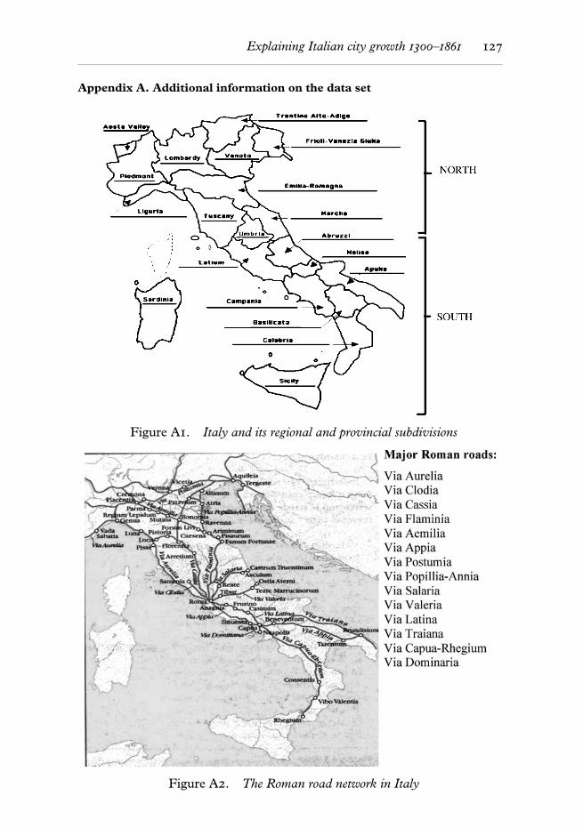
Explaining Italian city growth 1300–1861 127
Appendix A. Additional information on the data set
Figure A1. Italy and its regional and provincial subdivisions
Figure A2. The Roman road network in Italy
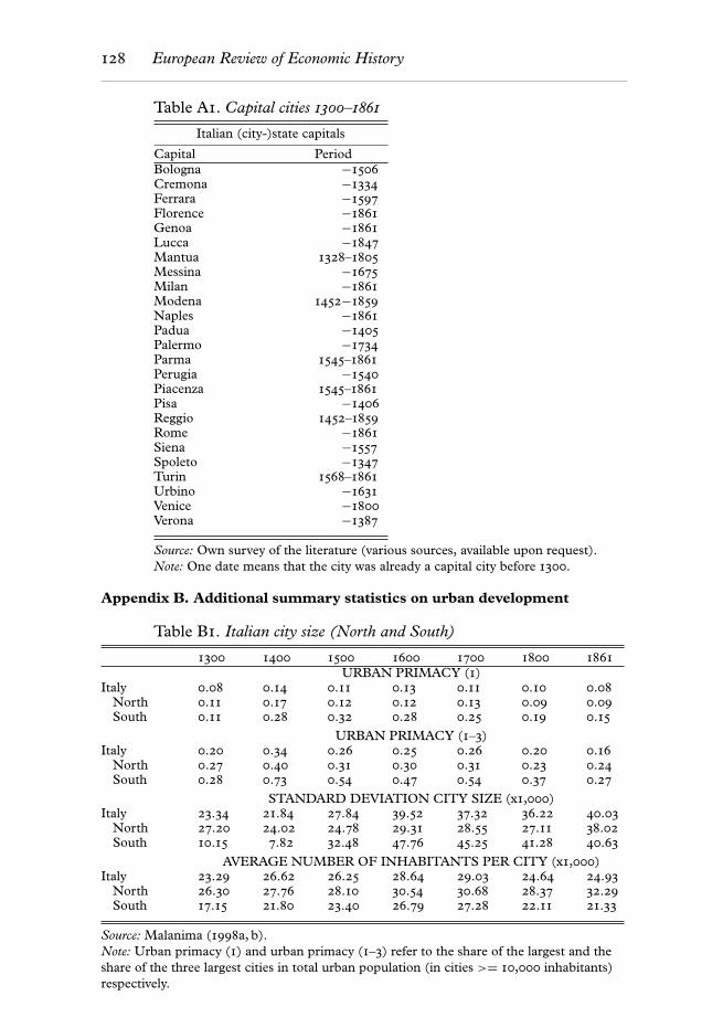
128 European Review of Economic History
Table A1. Capital cities 1300–1861
Italian (city-)state capitals
Capital PeriodBologna −1506Cremona −1334Ferrara −1597Florence −1861Genoa −1861Lucca −1847Mantua 1328–1805Messina −1675Milan −1861Modena 1452−1859Naples −1861Padua −1405Palermo −1734Parma 1545–1861Perugia −1540Piacenza 1545–1861Pisa −1406Reggio 1452–1859Rome −1861Siena −1557Spoleto −1347Turin 1568–1861Urbino −1631Venice −1800Verona −1387
Source: Own survey of the literature (various sources, available upon request).Note: One date means that the city was already a capital city before 1300.
Appendix B. Additional summary statistics on urban development
Table B1. Italian city size (North and South)
1300 1400 1500 1600 1700 1800 1861URBAN PRIMACY (1)
Italy 0.08 0.14 0.11 0.13 0.11 0.10 0.08North 0.11 0.17 0.12 0.12 0.13 0.09 0.09South 0.11 0.28 0.32 0.28 0.25 0.19 0.15
URBAN PRIMACY (1–3)Italy 0.20 0.34 0.26 0.25 0.26 0.20 0.16
North 0.27 0.40 0.31 0.30 0.31 0.23 0.24South 0.28 0.73 0.54 0.47 0.54 0.37 0.27
STANDARD DEVIATION CITY SIZE (x1,000)Italy 23.34 21.84 27.84 39.52 37.32 36.22 40.03
North 27.20 24.02 24.78 29.31 28.55 27.11 38.02South 10.15 7.82 32.48 47.76 45.25 41.28 40.63
AVERAGE NUMBER OF INHABITANTS PER CITY (x1,000)Italy 23.29 26.62 26.25 28.64 29.03 24.64 24.93
North 26.30 27.76 28.10 30.54 30.68 28.37 32.29South 17.15 21.80 23.40 26.79 27.28 22.11 21.33
Source: Malanima (1998a, b).Note: Urban primacy (1) and urban primacy (1–3) refer to the share of the largest and theshare of the three largest cities in total urban population (in cities >= 10,000 inhabitants)respectively.
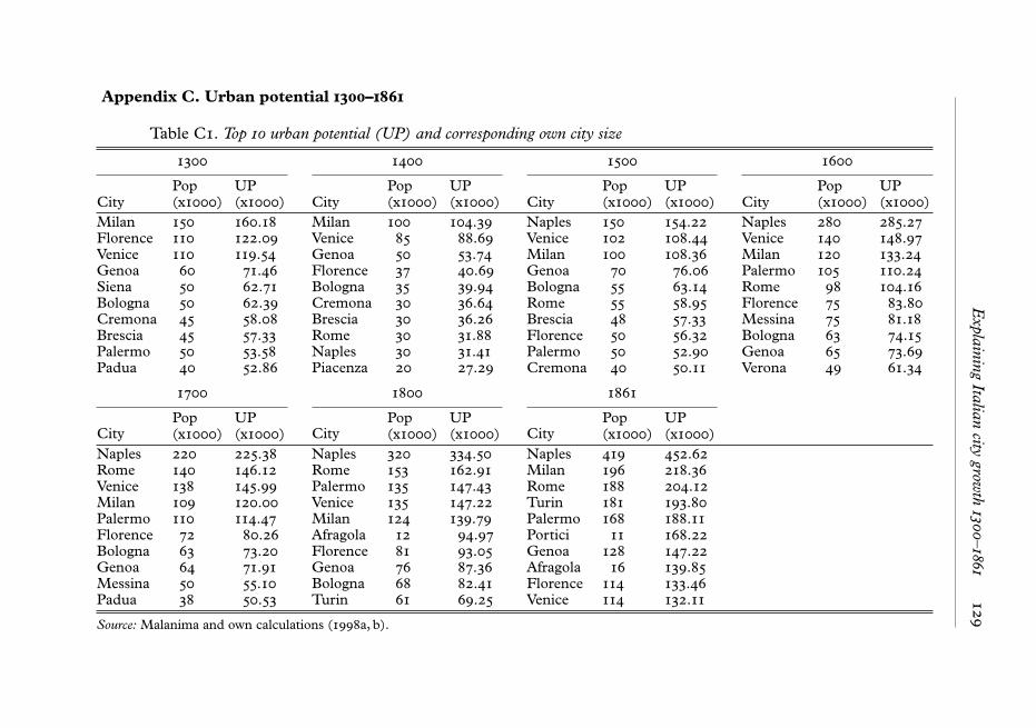
Explaining
Italiancity
growth
1300–
1861129
Appendix C. Urban potential 1300–1861
Table C1. Top 10 urban potential (UP) and corresponding own city size
1300 1400 1500 1600
CityPop(x1000)
UP(x1000) City
Pop(x1000)
UP(x1000) City
Pop(x1000)
UP(x1000) City
Pop(x1000)
UP(x1000)
Milan 150 160.18 Milan 100 104.39 Naples 150 154.22 Naples 280 285.27Florence 110 122.09 Venice 85 88.69 Venice 102 108.44 Venice 140 148.97Venice 110 119.54 Genoa 50 53.74 Milan 100 108.36 Milan 120 133.24Genoa 60 71.46 Florence 37 40.69 Genoa 70 76.06 Palermo 105 110.24Siena 50 62.71 Bologna 35 39.94 Bologna 55 63.14 Rome 98 104.16Bologna 50 62.39 Cremona 30 36.64 Rome 55 58.95 Florence 75 83.80Cremona 45 58.08 Brescia 30 36.26 Brescia 48 57.33 Messina 75 81.18Brescia 45 57.33 Rome 30 31.88 Florence 50 56.32 Bologna 63 74.15Palermo 50 53.58 Naples 30 31.41 Palermo 50 52.90 Genoa 65 73.69Padua 40 52.86 Piacenza 20 27.29 Cremona 40 50.11 Verona 49 61.34
1700 1800 1861
CityPop(x1000)
UP(x1000) City
Pop(x1000)
UP(x1000) City
Pop(x1000)
UP(x1000)
Naples 220 225.38 Naples 320 334.50 Naples 419 452.62Rome 140 146.12 Rome 153 162.91 Milan 196 218.36Venice 138 145.99 Palermo 135 147.43 Rome 188 204.12Milan 109 120.00 Venice 135 147.22 Turin 181 193.80Palermo 110 114.47 Milan 124 139.79 Palermo 168 188.11Florence 72 80.26 Afragola 12 94.97 Portici 11 168.22Bologna 63 73.20 Florence 81 93.05 Genoa 128 147.22Genoa 64 71.91 Genoa 76 87.36 Afragola 16 139.85Messina 50 55.10 Bologna 68 82.41 Florence 114 133.46Padua 38 50.53 Turin 61 69.25 Venice 114 132.11
Source: Malanima and own calculations (1998a, b).
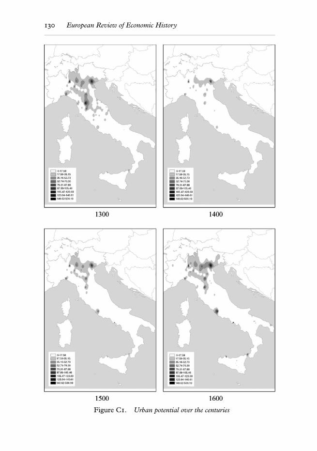
130 European Review of Economic History
Figure C1. Urban potential over the centuries
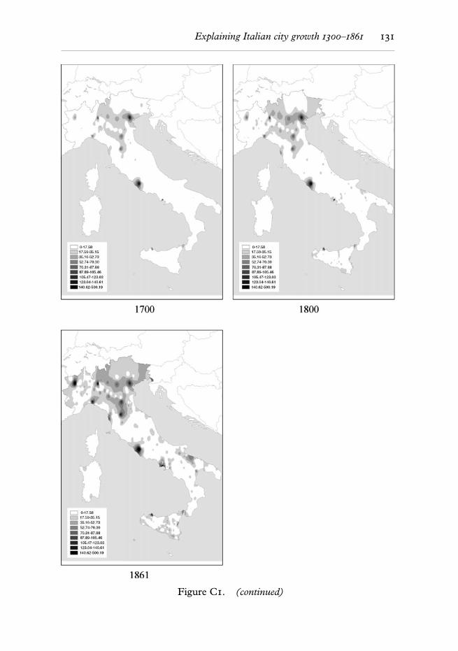
Explaining Italian city growth 1300–1861 131
Figure C1. (continued)