polynomial interpolation of minimal degree

Numer. Math. (1997) 78: 59–85 NumerischeMathematikc© Springer-Verlag 1997

Electronic Edition

Polynomial interpolation of minimal degree

Thomas Sauer

Mathematical Institute, University Erlangen–Nuremberg, Bismarckstr. 112 , D-90537 Erlangen, Ger-

many; e-mail: [email protected]

Received June 9, 1995 / Revised version received June 26, 1996

Dedicated to Prof. H. Berens on the occasion of his 60th birthday

Summary. Minimal degree interpolation spaces with respect to a finite set ofpoints are subspaces of multivariate polynomials of least possible degree forwhich Lagrange interpolation with respect to the given points is uniquely solvableand degree reducing. This is a generalization of the concept of least interpolationintroduced by de Boor and Ron. This paper investigates the behavior of Lagrangeinterpolation with respect to these spaces, giving a Newton interpolation methodand a remainder formula for the error of interpolation. Moreover, a special mini-mal degree interpolation space will be introduced which is particularly beneficialfrom the numerical point of view.

Mathematics Subject Classification (1991):65D10, 41A05, 41A10

1. Introduction

Given someN ∈ N0, a linear subspaceP ⊂ C(Rd) of dimensionN + 1 anda set of N + 1 pairwise distinct points, sayXN = {x0, . . . , xN} ⊂ R

d, theLagrange interpolation problemaddresses the question of finding, for any givenf : Rd → R, an elementP ∈ P which matchesf at XN ; i.e.,

P(xi ) = f (xi ), i = 0, . . . ,N .

The “simplest” example for such a spaceP , which can also be treated nu-merically in a suitable way, is whenP ⊂ Πd, whereΠd is the space of allpolynomials ind variables. It is well-known that in the univariate case the La-grange interpolation problem with respect toN + 1 distinct points is alwayspoised, i.e., uniquely solvable, if one takesP to be the space of all polynomialsof degree less than or equal toN . In several variables, however, the situation ismuch more difficult. In order to successfully interpolate withΠd

n , the space ofall polynomials of total degree less than or equal ton, the number of the points

Numerische Mathematik Electronic Editionpage 59 of Numer. Math. (1997) 78: 59–85

60 Th. Sauer

has to match the dimension of the space which is(n+d

d

), so that only point sets

of a certain cardinality are admissible. And even if this is the case, there can bethe problem that the points lie on some algebraic surface of degreen, i.e., thereis some polynomialq of total degree at mostn which vanishes onXN .

To overcome this problem, there have been several approaches to find config-urations of points which guarantee the poisedness of the respective interpolationproblem. Investigations in this spirit emerge from a remarkable paper by Chungand Yao [7] and were extended, e.g., by Gasca and Maeztu [10]; an extensivesurvey about these methods has been provided by Gasca [9].

Unfortunately, in many cases the points are given a priori and cannot bedetermined or modified by the interpolation process; for example, if the datato be interpolated stem from some physical or “real world” measurements. Inthis respect, even the Lagrange interpolation problem with respect to points withvery regular structure (e.g., points on a rectangular grid) need not be poisedin Πd

n , regardless of whether the cardinalities match or not. Consequently, ifthere is no access to the points, the only way out is to choose the subspacePsuitably, such that one can uniquely interpolate at the given points. The firstapproach in this direction is the concept ofKergin interpolation, introduced byKergin [11]. Although his method of constructing an interpolating polynomialprovides a very nice closed form of the interpolating polynomial based on ageneralized Newton interpolation formula, as pointed out by Micchelli [15], ithas the drawback that the interpolating polynomial with respect toN + 1 pointshas degreeN and cannot be handled very well numerically. From that pointof view it is important to find appropriate spacesP (i.e., polynomial subspacesP ⊂ Πd such that interpolation with respect to the given point setXN is poisedin P ) which consist of polynomials of least possible degree. This question hasbeen considered by de Boor and Ron [3] who investigated it to great extent in aseries of papers ([5, 1, 2] to name a few). They introduced a particular polynomialsubspace which they called theleast choice. Among other properties to be listedlater, this space, which depends on the nodes of interpolation, provides threeintrinsic features:

1. The Lagrange interpolation problem with respect to the pointsXN is uniquelysolvable in this subspace.

2. This subspace is of minimal degree; i.e., if the subspace contains polynomialsof total degree less or equal ton and at least one polynomial of total degreen, then the Lagrange interpolation problem with respect toXN is unsolvablein any subspace ofΠd

n−1.3. Interpolation with respect to this space is degree reducing; i.e., if a polynomial

p has total degreek ≤ n, then its interpolant has degree at mostk.

It has been pointed out in [6] what distinguishes the least interpolation schemefrom arbitrary interpolation spaces with the above three properties.

This paper will approach the question of finding proper polynomial sub-spaces by considering all polynomial subspaces which satisfy the above three


Minimal degree interpolation 61

requirements and study Lagrange interpolation with respect to them. For thesespaces, which we will callminimal degree interpolation spaces, we will derivean analogy to the univariate Newton interpolation method as well as a remainderformula. In addition, we will provide a particular minimal degree interpolationspace which captures quite a few of the striking properties of the least interpolantfrom de Boor and Ron but combines it with “optimal” numerical behavior in thesense that it minimizes storage and arithmetic operations, which may make thespace useful for practical applications.

The paper is organized as follows: first we will formally introduce minimaldegree interpolation spaces in Sect. 2 and discuss some of their basic properties.In Sect. 3 we will consider some special examples of minimal interpolationspaces, among them the least interpolation of de Boor and Ron. The Newtonmethod and the remainder formula are the subject of Sect. 4, while in the finalSect. 5 we construct and investigate the particular minimal degree interpolationspace mentioned above, stating and verifying its properties.

We will use standard multiindex notation throughout the paper. For a multi-indexα = (α1, . . . , αd) ∈ Nd

0, we denote by|α| = α1 + · · · + αd the lengthof α.Moreover, we write

xα = ξα11 · · · ξαd

d , x = (ξ1, . . . , ξd) ∈ Rd, α ∈ Nd0,

for the monomials. The totalityxα, |α| ≤ n, spansΠdn ⊂ Πd, the space of all

polynomials of total degree less than or equal ton. We will order multiindicesin the most convenient way, namelygraded lexicographically, writing α ≺ βif either |α| < |β| or |α| = |β| and α appears earlier thanβ in the standardlexicographical ordering. The latter means that there is some 1≤ k ≤ d suchthatαi = βi , i = 1, . . . , k − 1, andαk < βk .

2. Minimal degree interpolation spaces

Let XN = {x0, . . . , xN} be a set ofN + 1 distinct points inRd. We say thatthe Lagrange interpolation problem with respect toXN is poisedin a subspaceP ⊂ Πd, if for any f : Rd → R there exist a uniqueP ∈ P such that

P(xi ) = f (xi ), i = 0, . . . ,N .

Clearly, this requires that dimP = N + 1. Suppose that the Lagrange inter-polation problem with respect toXN is poised inP (XN ) ⊂ Πd, where thenotationP (XN ) is used to emphasize the fact that the spaceP (XN ), whichadmits unique Lagrange interpolation atXN , depends onXN . By LP (XN )(f , ·)we denote the projection off on P (XN ), i.e., the interpolating polynomialLP (XN )(f , ·) ∈ P (XN ) such that

LP (XN )(f , xi ) = f (xi ), i = 0, . . . ,N .

Since polynomials of high degree are expensive in storage, unstable in evaluationand therefore inconvenient for numerical purposes, it is reasonable to request


62 Th. Sauer

that the spaceP (XN ) is chosen ofminimal degree, i.e., we takeP (XN ) ⊂ Πdn

wheren is the minimum of all admissible values. In other words,n is chosen insuch a way that the Lagrange interpolation problem with respect toXN is notpoised in any subspace ofΠd

n−1. Of course,n depends onXN and satisfies

n ≤ N ≤(

n + dd

)− 1,

wheren = N if and only if all the points are on a straight line and(n+d

d

)= N + 1

if and only if the Lagrange interpolation problem with respect toXN is poisedin Πd

n . The latter case has been treated in [20].The second requirement is that Lagrange interpolation with respect to the spaceP (XN ) is degree reducing, a property observed already by de Boor and Ron[3]. This means that fork ≤ n

p ∈ Πdk ⇒ LP (XN )p ∈ Πd

k ,

which is a desirable behavior of the projection operatorLP (XN ) on Πdn .

Summarizing these requirements, we state

Definition 1. Let a finite setXN = {x0, . . . , xN} of N +1 pairwise distinct pointsbe given. A subspaceP (XN ) ⊂ Πd is called aminimal degree interpolationspace of order n with respect toXN provided that

1. the Lagrange interpolation problem with respect toXN is poised inP (XN )⊂ Πd

n ,2. P (XN ) is of minimal degree with this property, i.e., there is no subspace of

Πdn−1 which admits unique interpolation atXN ,

3. Lagrange interpolation with respect toP (XN ) is degree reducing.

Next we introduce a Newton interpolation method forP (XN ), extendingthe one in [20]. For that purpose, let us briefly recall that this approach is basedon rearranging the pointsXN , N = dimΠd

n − 1, into {xβ : |β| ≤ n}, such thatthere are polynomialspα ∈ Πd

|α|, |α| ≤ n, which satisfy

pα(xβ) = δα,β , |β| ≤ |α| ≤ n.

The setsxk = {xα : |α| = k} are calledblocks. To extend this notion to minimaldegree interpolation spaces, we consider index setsIk ⊂ {α : |α| ≤ k} ⊂ N

d0,

k = 0, . . . , n, andI−1 = ∅ for convenience, which satisfy

I0 ⊂ I1 ⊂ · · · ⊂ In and Ik \ Ik−1 ⊂ {α : |α| = k} , k = 0, . . . , n.(1)

The complements of these sets,I ′k := {α : |α| ≤ k} \ Ik , k = 0, . . . , n, then arenested as well. We say thatP ⊂ Πd

n admits aNewton basis of order n withrespect toXN , if there exists a system of index setsI = (I0, . . . , In), satisfying(1), such that

1. In \ In−1 /= ∅,



2. the points inXN can be re-indexed asXN = {xβ : β ∈ In}; in particular,#In = dimP (XN ) = N + 1,

3. there exists a basispα ∈ Πd|α|, α ∈ In, of P (XN ) such that

pα(xβ) = δα,β , β ∈ I|α|, α ∈ In,(2)

4. there exist polynomialsp⊥α ∈ Πd|α|, α ∈ I ′n, such that

p⊥α (XN ) = 0(3)

andΠd

n = span{pα : α ∈ In} ⊕ span{

p⊥α : α ∈ I ′n}.(4)

The polynomialspα, α ∈ In, are called theNewton fundamental polynomialswithrespect toXN in P (XN ). It is easily seen that the Lagrange interpolation prob-lem with respect toXN is poised inP (XN ) if there exist Newton fundamentalpolynomials forP (XN ) which satisfy (2) after re-indexingXN properly. Therespectiveblocksof points for such a Newton basis are the sets

xk := {xα : α ∈ Ik \ Ik−1} , k = 0, . . . , n.

The relation between minimal degree interpolation spaces and spaces whichadmit a Newton basis is now as close as can be, in view of

Theorem 1. A subspaceP ⊂ Πd is a minimal degree interpolation space oforder n with respect toXN if and only if there exists a Newton basis of order nwith respect toXN for P .

Proof. Assume thatP ⊂ Πdn is a minimal degree interpolation space of order

n with respect toXN . Let Q ={

q ∈ Πd : q(XN ) = 0}

denote the ideal of allpolynomials which annihilateXN and defineQk = Q ∩Πd

k , k ∈ N0. SincePis an interpolation space we have

Πdn = P ⊕ Qn.

SinceP is degree reducing, it follows thatΠdk = Pk ⊕Qk as well,k = 0, . . . , n,

wherePk := P ∩Πdk . This implies that there exists agraded basisfor P . Thus

we define the system of nested index setsI = (I0, . . . , In) in such a way that#Ik = dimPk , and write the graded basis as{φα : α ∈ Ik , k = 0, . . . , n}. Notethat this is trivially possible since the only requirements for the index system arebeing nested and having proper cardinality at each level. In order to obtain theNewton fundamental polynomials we then apply the “orthogonalization” processfrom [20] (see also [18]) to the polynomialsφα, α ∈ In, which also re-indexes thepoints inXN in an appropriate way. The polynomialsp⊥α , α ∈ I ′n, are obtainedsimilarly by taking any graded basis of the vector spaceQn and attaching theindices fromI ′ = (I ′0, . . . , I

′n) to it.

Conversely, it is obvious that the existence of a Newton basis forP impliespoisedness. To verify the minimal degree property we make use of the factthat the assumptionIn \ In−1 /= ∅ implies that dimPn−1 < dimPn = N + 1.


64 Th. Sauer

Due to the requirements on a Newton basis we have the representationΠdn−1 =

span{φα : |α| ≤ n − 1}, where

φα =

{pα if α ∈ In−1,p⊥α if α ∈ I ′n−1,

|α| ≤ n − 1.

But then the Vandermonde matrix

Vn−1 = [φα (xi )] i =0,...,N , |α|≤n−1

contains a zero column[φα(xi )] i =0,...,N wheneverα ∈ I ′n−1 and thereforerank Vn−1 ≤ #In−1 = dimPn−1 < N + 1, from which we conclude that theLagrange interpolation problem with respect toXn is not poised inΠd

n−1. Toprove the degree reducing property, choose anyp ∈ Πd

k , k ≤ n. Thenp can bewritten as

p(x) =∑α∈Ik

cαpα(x) +∑β∈I ′k

cβp⊥β (x),

and thus

LP (p, x) =∑α∈Ik

cαLP (pα, x) +∑β∈I ′k

cβLP (p⊥α , x) =∑α∈Ik

cαpα,

sinceLP (pα, x) = pα(x) andLP (p⊥α , x) = 0.�

The idea of Newton interpolation is straightforward: we definePk(XN ) asP (XN ) ∩Πd

k and letLkf ∈ Pk be the interpolating polynomial with respect tothe points{xα : α ∈ Ik}, k = 0, . . . , n. Then, for anyf : XN → R we generatethe interpolating polynomialLn(f , x) successively via

Lk+1(f , x) = Lk(f , x) + Lk+1 (f − Lkf , x) , k = 0, . . . , n − 1,

where the “additional” or “refining” informationLk+1 (f − Lkf , x) is a linear com-bination ofpα, α ∈ Ik+1 \ Ik , interpolating the error of the previous interpolationsteps. We will describe this method in detail in Section 4 where we also de-rive an error formula for minimal degree interpolation. To assure that the aboveprocedure always works we define

Jk := Ik \ Ik−1, J ′k := I ′k \ I ′k−1, k = 0, . . . , n,(5)

and state the following observation:

Proposition 1. If P (XN ) is a minimal degree interpolation space with respectto XN then the sets Jk, k = 0, . . . , n, of the respective Newton basis satisfy

Jk /= ∅, k = 0, . . . , n.



Proof. For an arbitrary graded basis ofΠdn , sayφα ∈ Πd

|α|, |α| ≤ n, let us again

consider the generalized (N + 1)× (k+dd

)Vandermonde matricesVk of order k,

k = 0, . . . , n, defined by

Vk(XN ) = [φα(xi )] i =0,...,N , |α|≤k , k = 0, . . . , n.

Note that the numbers rankVk , k = 0, . . . , n, are independentof the choice ofthe basis polynomialsφα, |α| ≤ n, as long as these are a graded basis ofΠd

n .SinceP (XN ) is a minimal degree interpolation space, we have

rank V0 ≤ rank V1 ≤ · · · ≤ rank Vn−1 < rank Vn = N + 1,(6)

where the strict inequality at the end stems from minimality. Now assume that forsomek < n we haveJk = ∅, or, in other words,J ′k = {α : |α| = k}. Consequently,Πd

k = span{

p⊥α : |α| = k}

+ Πdk−1 and therefore there exist coefficientscα,β ,

|α| = |β| = k, and polynomialsqα ∈ Πdn such that

xα =∑|β|=k

cα,β p⊥β (x) + qα(x), |α| = k.

Thus, the polynomialsφα := (·)α−qα, |α| = k, satisfyφα ∈ span{

p⊥α : α ∈ Jk}

,henceφα(XN ) = 0, |α| = k, which carries over to the polynomialsψα,β(x) =xβφα(x), |α| = k, |β| ≤ n − k. Moreover,

Πdn = span{(·)α : |α| < k} ⊕ span{ψα,β : |α| = k, |β| ≤ n − k}.

Thus, there is a graded basisφα of Πdn such thatφα(XN ) = 0 if |α| ≥ k. But

this implies thatrank Vk−1 = rank Vk = · · · = rank Vn,

contradicting (6).�

3. Special examples

Example 1.The first and most prominent example of a minimal degree interpo-lation space is theleast interpolationintroduced and extensively investigated byde Boor and Ron [3]. They started with explicitly constructing the least interpo-lation spacePl (XN ), according to some arbitrary given set of pointsXN , suchthat interpolation with respect toXN is poised inPl (XN ), and then proved thatit possesses the minimal degree property. See also [6] for a comparison betweenthe least interpolation space and general minimal degree interpolation spaces.They characterized the least interpolation space, which is uniquely determinedthrough the setXN , by means of the kernels of certain homogeneous differentialoperators. Precisely,Pl (XN ) is the unique minimal degree interpolation spacewhich satisfies

Pl (XN ) =⋂

q(X )=0

kern q↑(D),(7)


66 Th. Sauer

whereq↑, in the notation of de Boor and Ron, denotes theleading termof q,defined in the following way: assume thatq has degreen, thenq↑ is the uniquehomogeneous polynomial of degreen such that

q(x)− q↑(x) ∈ Πdn−1.

For information on how to constructPl (XN ) and the interpolating polynomialin numerical practice, see [1, 5].

Among several other remaining properties, this particular space turns out tobe scale invariant and shift invariant, i.e.,

Pl (XN ) = Pl (cXN − y), c ∈ R, c /= 0, y ∈ Rd,

wherecX − y = {cx0 − y, . . . , cxN−1 − y} .

Since minimal degree interpolation spaces cannot be rotationally invariant ingeneral, this is the strongest coordinate system independence to be expected.Also note that shift and scale invariance implies thatPl (XN ) is closed underderivation.

Example 2.To work with polynomials practically, one usually stores and manip-ulates their coefficients with respect to some basis and the most convenient (butnot numerically most stable) basis to be used are the monomialsxα, α ∈ Nd

0.Since the requirements on storage and the number of operations necessary tomanipulate polynomials depend on the number of basis functions necessary torepresent the subspaceP (XN ), it can be beneficial to find a minimal degreeinterpolation space which uses as few basis functions as possible. To illustratethis idea, let us first consider the following extremal situation:Suppose the pointsx0, . . . , xN are all on a straight line, i.e.,xj = x0 + λj a,j = 1, . . . ,N , for some 0/= a ∈ Rd and pairwise distinctλj ∈ R, j = 1, . . . ,N .Assume in addition thataj /= 0, j = 1, . . . , d and let ` ∈ Πd

1 be the linearpolynomial

`(x) = 〈a, x〉, x ∈ Rd.

Then one minimal degree interpolation space with respect toXN (which is eventhe least interpolation space for that configuration of points) is spanned by thepowers of`, `k(x), k = 0, . . . ,N , and the Newton fundamental polynomials are

pk(x) =`(x − x0) · · · `(x − xk−1)`(xk − x0) · · · `(xk − xk−1)

, k = 0, . . . ,N .

Note that each of these polynomials has(k+d

d

)coefficients with respect to the

monomials due to the assumption that all coefficientsaj are nonzero; hence,a “typical” interpolation polynomial for this situation will have to store andmanipulate

(N+dd

)= O(N d) coefficients with respect to the monomial basis. Also

the evaluation of these polynomials requires access toO(N d) coefficients whichmakes it ineffective compared to the dimension of the space which is onlyN +1.



Note that this problem is not a consequence of choosing the monomials as a basis:“usually” (i.e., up to set of measure zero) the coefficient vector of a multivariateinterpolating polynomial with respect to any basis is densely filled with entries,regardless of the underlying basis.

Example 3.From the preceding example we see that it may be beneficial fornumerical purposes to find minimal degree interpolation spaces which can bedescribed by as few generic basis functions as possible; though not being the bestpossible choice from the point of view of numerical stability, the monomials arestill the simplest and most common choice for a generic basis of polynomials.

As already mentioned, there is always a subspace ofΠdN such that in this

subspace the Lagrange interpolation problem with respect to givenN + 1 pointsx0, . . . , xN is poised – one may take, for example, the Kergin interpolant. Thisimplies that for any choice of pairwise distinct points the (N + 1)× (N+d

d

)Van-

dermonde matrix (which is no more a square matrix ford > 1)

VN =[xαi]

i =0,...,N , |α|≤N

always has rankN +1. Hence, there must be an (N +1)×(N +1) sub-matrix ofVN

with non-vanishing determinant; in other words, there always exists a subspacespanned byN + 1 monomials, where the Lagrange interpolation problem withrespect toXN is poised. Among these spaces spanned by certain monomials,there will also be one (and in general several) subspace(s) of minimal degree.We will refer to minimal degree interpolation spaces which are spanned byN +1monomials asminimal degree interpolation with minimal monomials. However,we will need further requirements to single out a unique minimal degree inter-polation space with minimal monomials. We will make this more precisely inSect. 5, where we use this remaining degree of freedom to construct a minimaldegree interpolation space which combines the minimal monomials property withthe invariance properties of least interpolation.

Example 4.The final idea to specialize a minimal degree interpolation space isto introduce additional points in such a way that the original points and the addedones give rise to a Lagrange interpolation problem which is poised inΠd

n , wherenis the specific minimal degree. For that purpose let us recall thatP (XN ) ⊂ Πd

n

already admits unique Lagrange interpolation; now, if we consider the vectorspaceQn, on the other hand, then it is well–known (see for instance [19]) thatthe Lagrange interpolation problem with respect to a proper number of points ispoised except for a set of measure zero. Letxα, α ∈ I ′n, be such a set of points(their number is correct since the dimension ofQn equals the cardinality ofI ′n),then it is easily seen that the Lagrange interpolation problem with respect to

{xα : α ∈ In} ∪ {xα : α ∈ I ′n}is poised inΠd

n – this is an immediate consequence of the fact thatΠdn =

P (XN ) ⊕ Qn. Choosing a reasonable Newton basis in bothP (XN ) and Qn

we can reformulate this process as follows: we add pointsxα, α ∈ I ′n, such that


68 Th. Sauer

there are polynomialspα, α ∈ In, andp⊥α , α ∈ I ′n, such thatp⊥α (X ) = 0 and, inaddition

pα(xβ) = δα,β , |β| ≤ |α|, α ∈ Ik ,(8)

and, respectively,

p⊥α (xβ) = δα,β , |β| ≤ |α|, α ∈ I ′k .(9)

Of course, there is again freedom in choosing the additional points since the aboveextension is possible for almost all choices ofxα, α ∈ I ′n. This type of minimaldegree interpolation, referred to asminimal degree interpolation with additionalpoints, provides a particularly nice and simple remainder formula which will begiven in (23).

4. Finite difference and remainder formula

In the caseP (XN ) = Πdn for somen ∈ N, there are two remainder formulae

which are valid for all sets of pointsXN that do not lie on an algebraic surfaceof degreen: the first one is due to Ciarlet [8] and is based on amultipoint Taylorexpansion, while the more recent one, developed in [20], is obtained from aNewton interpolation scheme. In this section we will extend the latter result tominimal degree interpolation spaces.

It has to be remarked here that Newton formulae for special configurationsof points have been given and investigated before, cf., for example [12, 21, 17].These methods have in common that they transform the structure of the datapoints to a rectangular grid and then use a tensor product approach. However,the Newton interpolation to be described here is based on a finite difference ap-proach for minimal degree interpolation which is very much similar to the methodintroduced in [20]. In addition to its theoretic use for deriving the remainder for-mula, the Newton method also offers a good tool in practical computations: itnot only provides a fast method to compute the interpolating polynomial withless memory consumption, but also shows superior numerical robustness if thefunction is sufficiently smooth (see [18]). The key tool for the derivation of theNewton method is thefinite differenceλk [x0, . . . , xk−1, x], k = 0, . . . , n, whichis defined recursively as

λ0[x]f := f (x)(10)

λk+1[x0, . . . , xk , x]f := λk [x0, . . . , xk−1, x]f(11)

−∑α∈Jk

λk [x0, . . . , xk−1, xα]f · pα(x).

It has been pointed out in [20] that in cased = 1 this difference coincides witha re-normalized version of the classical divided differencef [. . .]; precisely:

λn+1[x0, . . . , xn, x]f = f [x0, . . . , xn, x](x − x0) · · · (x − xn).

Indeed, this difference plays a crucial role in describing the interpolating poly-nomial and the error of interpolation.



Theorem 2. For a minimal degree interpolation space with Newton fundamentalpolynomials pα, α ∈ In, the interpolating polynomial for a function f is given by

Ln(f , x) =∑α∈In

λ|α|[x0, . . . , x|α|−1, xα]f · pα(x).(12)

Moreover,f (x)− Ln(f , x) = λn+1[x0, . . . , xn, x]f .(13)

Proof. We will prove that equations (12) and (13) both hold withn replaced byk, k = 0, . . . , n, whereLk corresponds to interpolating at the pointsxα, α ∈ Ik ,with the span of the polynomialspα, α ∈ Ik . This will be be done by inductionon k. Indeed, ifk = 0, then (12) and (13) read

L0(f , x) = f (x0), f (x)− L0(x) = λ1[x0, x]f = f (x)− f (x0).

So, suppose that for somek < n, the equations are already verified. Since thepolynomialspα, α ∈ Jk+1 (recall:Jk+1 = Ik+1\ Ik), vanish inxβ , β ∈ Ik , we obtainthat forβ ∈ Ik ∑

α∈Ik+1

λ|α|[x0, . . . , x|α|−1, xα]f · pα(xβ)

=∑α∈Ik

λ|α|[x0, . . . , x|α|−1, xα]f · pα(xβ)

= Lk(f , xβ) = f (xβ).

For β ∈ Jk+1 we use (13), (12) and the fact thatpα(xβ) = δα,β , α ∈ Jk+1, tocompute

f (xβ) = Lk(f , xβ) + f (xβ)− Lk(f , xβ)

= Lk(f , xβ) + λk+1[x0, . . . , xk , xβ ]f

=∑α∈Ik

λ|α|[x0, . . . , x|α|−1, xα]f · pα(xβ)

+∑α∈Jk+1

λk+1[x0, . . . , xk , xα]f · pα(xβ)

=∑α∈Ik+1

λk+1[x0, . . . , xk , xα]f · pα(xβ).

Hence, (12) holds fork + 1. Using the recursive definition of the finite differencefinally yields

λk+2[x0, . . . , xk+1, x]f

= λk+1[x0, . . . , xk , x]f −∑α∈Jk+1

λk+1[x0, . . . , xk , xα]f · pα(x)

= f (x)− Lk(f , x)− (Lk+1(f , x)− Lk(f , x))

= f (x)− Lk+1(f , x),

which is (13) fork + 1.�


70 Th. Sauer

Of course, one could also introduce the finite difference via (13). Then (12)is obvious, but one has to prove the recurrence relation (11) instead. Since theproof of the remainder formula uses induction based on this recurrence, the aboveway to introduce the finite difference is more convenient here.

To formulate and establish the remainder formula for minimal degree inter-polation, we have to introduce some additional notation. First, let us generalizethe notion of a path as defined in [20] to paths inIn. A path in In is a vector ofmultiindices of increasing length, which has the form

µ = (µ0, . . . , µn), µk ∈ Jk , k = 0, . . . , n.

Let Λn denote the totality of all those paths. The name “path” stems from theimage of walking through the set of multiindices inIn, ascending to higher levelin each step and passing exactly one multiindex on each level. Note that thisnotion still is reasonable because of Proposition 1 which certifies that at eachlevel there is at least one multiindex where the path can pass through. In otherwords: there are no “broken” paths or “jumps”. To each pathµ ∈ Λn we associatethe well–defined numbers

πµ(xµ) =n−1∏i =0

pµi (xµi +1),

a homogeneousn–th order differential operator

Dnxµ = Dxµn−xµn−1

· · ·Dxµ1−xµ0,

as well as the set of points on the path

xµ = {xµ0, . . . , xµn} .

Finally, let us recall the notion of a simplex spline: given anyn +1≥ d +1 knotsv0, . . . , vn ∈ Rd, the simplex spline M(x|v0, . . . , vn) is the distribution definedby ∫

Rd

f (x) M (x|v0, . . . , vn) dx(14)

= (n − d)!∫

Sn

f (σ0v0 + · · · + σnv

n)dσ, f ∈ C(Rd),

where

Sn := {σ = (σ0, . . . , σn) : σi ≥ 0, σ0 + · · · + σn = 1} .The most important property for our present purposes is the formula for direc-tional derivatives, derived, among other important facts about simplex splines,by Micchelli [16]:



DyM (x|v0, . . . , vn) =n∑

j =0

µj M (x|v0, . . . , vj−1, vj +1, . . . , vn),(15)

y =n∑

j =0

µj vj ,

n∑j =0

µj = 0.

We will need this in the more special version

Dvi−vj M (x|v0, . . . , vn)

= M (x|v0, . . . , vi−1, vi +1, . . . , vn)−M (x|v0, . . . , vj−1, vj +1, . . . , vn),(16)

0≤ i , j ≤ n.

Before giving the integral representation of the finite difference for any min-imal degree interpolation space, let us have a brief look at the representationformula from [20] for the special case of a Lagrange interpolation problem beingpoised inΠd

n . The formula reads as

λn+1[x0, . . . , xn, x]f =∑µ∈Λn

pµn (x)πµ(xµ)∫Rd

Dx−xµnDn

xµ f (t)M (t |xµ, x) dt.

The differential operator under the integral is of ordern + 1 and hence, the aboveexpression vanishes on all polynomials of degree less than or equal ton. Sincewe have, due to (13), that

λn+1[x0, . . . , xn, x]p⊥α = p⊥α (x)− Ln(p⊥α , x) = p⊥α (x), α ∈ I ′n,

there have to be additional terms in the remainder formula for minimal degreeinterpolation which are responsible for the reproduction of the polynomialsp⊥α .For their description, we have to define the directionsdα,β ∈ Rd, α ∈ Jk , β ∈ I ′k+1as the unique solutions of the vector interpolation problem∑β∈I ′k+1

dα,β p⊥β (x) = pα(x) (x − xα)−∑β∈Jk+1

pβ(x)pα(xβ)(xβ − xα

), α ∈ Jk .

(17)

Lemma 1. The interpolation problem (17) is uniquely solvable for eachα ∈ Jk,k = 0, . . . , n − 1.

Proof. Since the polynomial on the right-hand side is a polynomial of degreek + 1, it suffices to show that

ϕ(x) = pα(x) (x − xα)−∑β∈Jk+1


)satisfiesϕ(xγ) = 0, γ ∈ Ik+1. This is obvious forγ ∈ Ik with γ /= α, and also forγ = α, since then both terms vanish. In the remaining casesγ ∈ Jk+1 we have

ϕ(xγ) = pα(xγ)(xγ − xα

)− 1 · pα(xγ)(xγ − xα

)= 0.

because ofpβ(xγ) = δβ,γ . Hence,ϕ(x) belongs to the span ofp⊥β , β ∈ I ′k+1 andcan therefore be uniquely represented as required in (17).�


72 Th. Sauer

Now we are in position to formulate the remainder formula for a minimaldegree interpolation space as

Theorem 3. Let P (XN ) be a minimal degree interpolation space of degree n.Then

f (x)− Ln(f , x) = λn+1[x0, . . . , xn, x]f

=∑µ∈Λn


Dx−xµnDn

xµ f (t)M (t |xµ, x)dt(18)

+∑β∈I ′n

p⊥β (x)∫Rd

n∑j =|β|

∑µ∈Λj−1

πµ(xµ)Ddµj−1,βDj−1

xµ f (t)M (t |xµ, x)dt.

Proof. The proof will use induction onk to prove that for any 0≤ k ≤ n

λk+1[x0, . . . , xk , x]f

=∑µ∈Λk

pµk (x)πµ(xµ)∫Rd

Dx−xµkDk


+k∑

j =1

∑µ∈Λj−1

∑β∈I ′j

p⊥β (x)πµ(xµ)∫Rd

Ddµj−1,βDj−1

xµ f (t)M (t |xµ, x)dt,

from which (18) follows by settingk = n and rearranging summation and inte-gration in the second term.

Since (0, . . . , 0) ∈ I0, equation (19) withk = 0 reads as

λ1[x0, x]f = f (x)− f (x0) =∫Rd

Dx−x0f (t)M (t |x0, x)dt,

which is clearly true. Hence, suppose that for some 0≤ k < n equation (19) hasalready been proved. In particular, we know that forβ ∈ Jk+1

λk+1[x0, . . . , xk , xβ ]f(20)

=∑µ∈Λk

pµk (xβ)πµ(xµ)∫Rd

Dxβ−xµkDk

xµ f (t)M (t |xµ, xβ)dt,

since the second term of (19) vanishes in all points ofXN by the definitionof the polynomialsp⊥α . Applying (17) and recalling the linearity of directionalderivatives then yields that forγ ∈ Jk

pγ(x)Dx−xγ =∑β∈Jk+1

pβ(x)pγ(xβ)Dxβ−xγ +∑β∈I ′k+1

p⊥β (x)Ddγ,β .(21)

Inserting this into (19) gives



λk+1[x0, . . . , xk , x]f

=∑µ∈Λk

∑β∈Jk+1

pβ(x)pµk (xβ)πµ(xµ)∫Rd

Dxβ−xµkDk

xµ f (t)M (t |xµ, x)dt

+∑µ∈Λk

∑β∈I ′k+1


Ddµk ,βDk


+k∑

j =1

∑µ∈Λj−1

∑β∈I ′j


Ddµj−1,βDj−1


=∑µ∈Λk

∑β∈Jk+1

pβ(x)pµn (xβ)πµ(xµ)∫Rd

Dxβ−xµkDk


+k+1∑j =1

∑µ∈Λj−1

∑β∈I ′j


Ddµj−1,βDj−1


and we substitute this and (20) into the recurrence relation (11) to obtain

λk+2[x0, . . . , xk+1, x]f

= λk+1[x0, . . . , xk , x]f −∑β∈Jk+1

λk+1[x0, . . . , xk , xβ ]f · pβ(x)

=∑µ∈Λk

∑β∈Jk+1

pβ(x)pµk (xβ)πµ(xµ)∫Rd

Dxβ−xµkDk


+k+1∑j =1

∑µ∈Λj−1

∑β∈I ′j


Ddµj−1,βDj−1


−∑β∈Jk+1

pβ(x)∑µ∈Λk

pµk (xβ)πµ(xµ)∫Rd

Dxβ−xµkDk

xµ f (t)M (t |xµ, xβ)dt

=∑µ∈Λk

∑β∈Jk+1

pβ(x)pµk (xβ)πµ(xµ)

×∫Rd

Dxβ−xµkDk

xµ f (t)(M (t |xµ, x)−M (t |xµ, xβ)

)dt

+k+1∑j =1

∑µ∈Λj−1

∑β∈I ′j


Ddµj−1,βDj−1


Since by (16)

M (t |xµ, x)−M (t |xµ, xβ) = Dxβ−xM (t |xµ, xβ , x),

we can apply partial integration to obtain

λk+2[x0, . . . , xk+1, x]f

=∑µ∈Λk

∑β∈Jk+1

pβ(x)pµk (xβ)πµ(xµ)


74 Th. Sauer

×∫Rd

Dx−xβDxβ−xµkDk

xµ f (t)M (t |xµ, xβ , x)dt

+k+1∑j =1

∑µ∈Λj−1

∑β∈I ′j


Ddµj−1,βDj−1


Writing µk+1 instead ofβ finally completes the induction.�

Looking at (18) we observe that then–th order differential operators

Dnβ =

n∑j =|β|

∑µ∈Λj−1

πµ(xµ)Ddµj−1,βDj−1

xµ , β ∈ I ′n,

are in general inhomogeneous. Thus, it is interesting to ask for minimal degreeinterpolation spaces whereDn

β is a homogeneousdifferential operator for allβ ∈ I ′n. For that purpose note thatDn

β has to have a component of order|β| forthe reproduction ofp⊥β . So the question is equivalent to asking whether thereexist minimal degree interpolation spaces such thatdγ,β = 0 if |β| ≤ |γ|. Theanswer is positive and a class of examples will be minimal degree interpolationwith additional points.

The derivation of a particularly simple formula for this case is based on thefact that we can give the coefficientsdα,β explicitly in

Lemma 2. Let the polynomials pα, α ∈ In, and p⊥α , α ∈ I ′n, satisfy (8) and (9).Then for anyα ∈ Jk, k ≤ n − 1,

pα(x) (x − xα)(22)

=∑β∈Jk+1


)+∑β∈J ′k+1

p⊥β (x)pα(xβ)(xβ − xα

).

Proof. The proof works in exactly the same way as the one of Lemma 1: it isagain easily verified that forx = xγ , |γ| ≤ k, both sides of (22) vanish andhave the same value forx = xγ , |γ| = k + 1. Since interpolation at the pointsxγ , |γ| ≤ k + 1, is unique inΠd

k+1, k = 0, . . . , n − 1, the polynomials have to beidentical.�

From (22) it now follows that

dα,β =

{0 |β| ≤ |α|,

pα(xβ)(xβ − xα

) |β| = |α| + 1,α ∈ In−1, β ∈ I ′n,

which enables us to give the remainder formula for a minimal degree interpolationspace with additional points.

Corollary 1. Let P (XN ) be a minimal degree interpolation space of degree nwith additional points. Then



f (x)− Ln(f , x) = λn+1[x0, . . . , xn, x]f

=∑µ∈Λn


Dx−xµnDn


+∑β∈I ′n

p⊥β (x)∫Rd

∑µ∈Λ|β|−1

pµn (xβ)πµ(xµ)

×Dxβ−xµnD |β|−1


5. Minimal monomials

In this section we will introduce and investigate a particular minimal degree in-terpolation spaceP ∗(XN ), spanned by a minimal number of monomials, whichare, moreover, nested in an appropriate way. We will see that this space com-bines properties of least interpolation with the practical advantage of minimalmemory consumption which makes it particularly useful for practical purposes.Some numerical details are also discussed at the end of this section.

5.1. Construction

Since the construction of the space is quite intricate and overshadowed by thenotation, let us first sketch an outline of the construction. The main idea is tochoose the monomials which span the interpolation space in such a way that therespective set of exponents,In, is a lower set; those play an important role inthe study of the multivariate Birkhoff interpolation problem (see e.g., [17, 13] or[14] for a more extensive survey). ThatIn is a lower set means that wheneverα ∈ In andβ ∈ Nn

0 satisfyα− β ∈ Nd0, thenβ ∈ In as well.

This property will be ensured by choosing the complement spacesQk , k =0, . . . , n, in such a way that they are spanned by polynomials which only havea single monomial with an exponent fromI ′n in their leading term, i.e., thepolynomialsp⊥α will be of the form xα + qα(x), qα ∈ P|α| + Πd

|α|−1, α ∈ I ′n.The crucial point of the construction is to build these polynomials and index setsin such a way thatI ′ := Nd

0 \ In ⊃ I ′n is an upper set(i.e., α ∈ I ′ implies thatα + β ∈ I ′, β ∈ Nd

0). This is possible due to the well–known fact thatQ is thepolynomial idealassociated to thefinite varietyXN (cf. [4]). Indeed, ifα ∈ I ′n,thenp⊥α (x) = xα + qα(x) belongs toQ and alsoξi p⊥α (x) = xα+ei

+ ξi qα(x) ∈ Q .In other words,α + ei belongs toI ′n as well and again the only exponent fromI ′n in the leading term ofξi p⊥α is α + ei . In view of this, it suffices to find theminimal indicesα ∈ I ′n, i.e., those elementsα ∈ I ′n which cannot be written asα = β + γ, β ∈ I ′n, γ ∈ Nd

0. These indices will be automatically determined inthe process of computing the Newton basis.

Let us now turn to the details of the construction. Still we assumeXN ={x0, . . . , xN} to be a finite set of pairwise distinct points. We claim that there


76 Th. Sauer

exists a minimal degree interpolation space of degree, sayn, which is spannedby xα, α ∈ In, and has the additional properties that the complementary indicessatisfy the following two conditions:

1. α ∈ I ′k , k < n, impliesα + ei ∈ I ′k+1, i = 1, . . . , d.2. the polynomialsp⊥α , α ∈ I ′n, satisfy

∂|β|

∂xβp⊥α = β! δα,β , α, β ∈ I ′n, |α| = |β|.(24)

Note that (24) is a reformulation of the fact that the only exponent fromI ′|α| in

the leading term ofp⊥α is α.We construct the spaceP ∗(XN ) by an inductional process onk = 0, . . . , n,

subsequently generating the index setsIk and I ′k as well as the point setsXk ={xα : α ∈ Ik} and the polynomialspα, α ∈ Ik , andp⊥α , α ∈ I ′k , respectively. Forconvenience we will write

P ∗k = span{pα : α ∈ Ik} , Qk = span

{p⊥α : α ∈ I ′k

}.

For k = 0 we only have to definep0 = 1, I0 = {0}, which fulfills all the require-ments. So, let us suppose that for somek, 0≤ k < n we already constructed asetIk of multiindices, Newton fundamental polynomialspα, α ∈ Ik , and the com-plementary basisp⊥α , α ∈ I ′k , with the above properties. Since the polynomialsξi · p⊥α (x), i = 1, . . . , d, α ∈ I ′k , also annihilateXN , we set

I ′k+1 = I ′k ∪{α + ei : i = 1, . . . , d, α ∈ I ′k

}, Ik+1 = {α : |α| ≤ k + 1} \ I ′k+1,

and p⊥α+ei (x) = ξi p⊥α (x), i = 1, . . . , d, α ∈ I ′k . If for someβ, |β| = k + 1, thereare several ways to writeβ in the form β = α + ei , 1 ≤ i ≤ d, α ∈ I ′k , thenwe choose the lexicographically largestα which satisfiesβ = α + ei for some0≤ i ≤ d. The polynomialsp⊥α , α ∈ J ′k+1, constructed this way are well–definedand vanish onXN .

Replacingn by k in (24) shows that the span ofp⊥α , α ∈ J ′k+1, has the samedimension as the span ofxα, α ∈ J ′k+1, and still satisfies (24) withk + 1 insteadof n. Hence, the polynomialsp⊥α , α ∈ I ′k+1, andxα, α ∈ Ik+1, define a basis ofΠd

k+1.Let Lk denote the interpolation operator with respect to the pointsxα, α ∈ Ik ,

and define forα ∈ Jk+1

φα(x) := xα − Lk ((·)α, x) .(25)

Clearly, these polynomials annihilateXk = {xα : α ∈ Ik}.For the polynomialsφα, α ∈ Jk+1, we now have to decide whether they “fallinto” to P ∗

k+1 or to Qk+1. For that purpose, we arrange the multiindicesα ∈ Jk+1

in lexicographical order and again proceed inductively. Let us assume that forsomeα ∈ Jk+1 we already obtained pointsxβ and polynomialspβ , β ∈ Jk+1,β ≺ α, which satisfy

pβ(xγ) = δβ,γ , γ ∈ Ik+1, β ∈ Jk+1, γ � β ≺ α.(26)



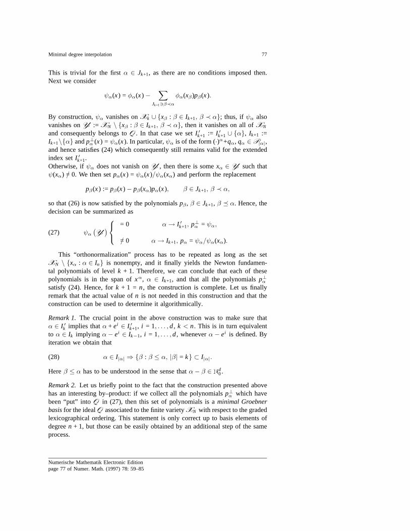
This is trivial for the firstα ∈ Jk+1, as there are no conditions imposed then.Next we consider

ψα(x) = φα(x)−∑

Jk+13β≺αφα(xβ)pβ(x).

By construction,ψα vanishes onXk ∪ {xβ : β ∈ Ik+1, β ≺ α}; thus, if ψα alsovanishes onY := XN \ {xβ : β ∈ Ik+1, β ≺ α}, then it vanishes on all ofXN

and consequently belongs toQ . In that case we setI ′k+1 := I ′k+1 ∪ {α}, Ik+1 :=Ik+1\{α} andp⊥α (x) = ψα(x). In particular,ψα is of the form (·)α+qα, qα ∈ P|α|,and hence satisfies (24) which consequently still remains valid for the extendedindex setI ′k+1.Otherwise, ifψα does not vanish onY , then there is somexα ∈ Y such thatψ(xα) /= 0. We then setpα(x) = ψα(x)/ψα(xα) and perform the replacement

pβ(x) := pβ(x)− pβ(xα)pα(x), β ∈ Jk+1, β ≺ α,

so that (26) is now satisfied by the polynomialspβ , β ∈ Jk+1, β � α. Hence, thedecision can be summarized as

ψα(Y)

= 0 α→ I ′k+1, p⊥α = ψα,

/= 0 α→ Ik+1, pα = ψα/ψα(xα).(27)

This “orthonormalization” process has to be repeated as long as the setXN \ {xα : α ∈ In} is nonempty, and it finally yields the Newton fundamen-tal polynomials of levelk + 1. Therefore, we can conclude that each of thesepolynomials is in the span ofxα, α ∈ Ik+1, and that all the polynomialsp⊥αsatisfy (24). Hence, fork + 1 = n, the construction is complete. Let us finallyremark that the actual value ofn is not needed in this construction and that theconstruction can be used to determine it algorithmically.

Remark 1.The crucial point in the above construction was to make sure thatα ∈ I ′k implies thatα + ei ∈ I ′k+1, i = 1, . . . , d, k < n. This is in turn equivalentto α ∈ Ik implying α− ei ∈ Ik−1, i = 1, . . . , d, wheneverα− ei is defined. Byiteration we obtain that

α ∈ I|α| ⇒ {β : β ≤ α, |β| = k} ⊂ I|α|.(28)

Hereβ ≤ α has to be understood in the sense thatα− β ∈ Nd0.

Remark 2.Let us briefly point to the fact that the construction presented abovehas an interesting by–product: if we collect all the polynomialsp⊥α which havebeen “put” intoQ in (27), then this set of polynomials is aminimal Groebnerbasisfor the idealQ associated to the finite varietyXN with respect to the gradedlexicographical ordering. This statement is only correct up to basis elements ofdegreen + 1, but those can be easily obtained by an additional step of the sameprocess.


78 Th. Sauer

Remark 3.We did not fix in (27) which particular element fromY to chooseas xα. This leaves room for several pivoting strategies. The straightforward nu-merical choice would be to take that element such that the absolute value ofψαat this point becomes maximal.

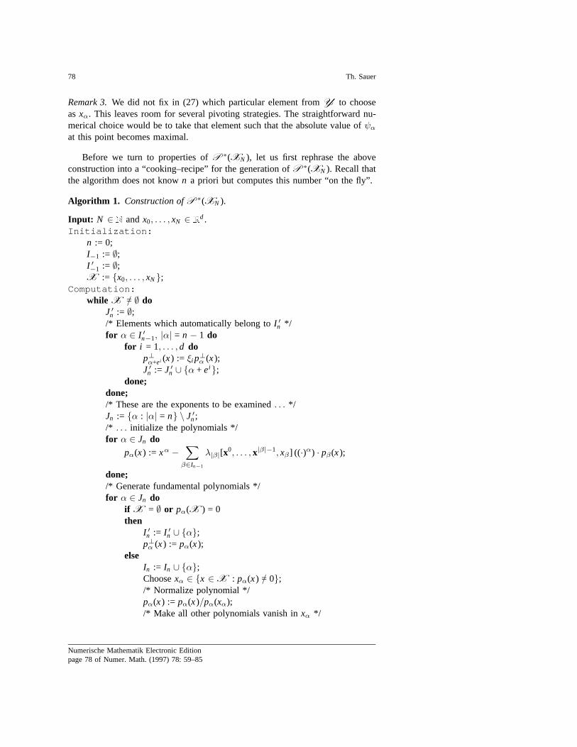
Before we turn to properties ofP ∗(XN ), let us first rephrase the aboveconstruction into a “cooking–recipe” for the generation ofP ∗(XN ). Recall thatthe algorithm does not known a priori but computes this number “on the fly”.

Algorithm 1. Construction ofP ∗(XN ).

Input: N ∈ N andx0, . . . , xN ∈ Rd.Initialization:

n := 0;I−1 := ∅;I ′−1 := ∅;X := {x0, . . . , xN};

Computation:while X /= ∅ do

J ′n := ∅;/* Elements which automatically belong toI ′n */for α ∈ I ′n−1, |α| = n − 1 do

for i = 1, . . . , d dop⊥α+ei (x) := ξi p⊥α (x);J ′n := J ′n ∪ {α + ei };

done;done;/* These are the exponents to be examined. . . */Jn := {α : |α| = n} \ J ′n;/* . . . initialize the polynomials */for α ∈ Jn do

pα(x) := xα −∑

β∈In−1

λ|β|[x0, . . . , x|β|−1, xβ ] ((·)α) · pβ(x);

done;/* Generate fundamental polynomials */for α ∈ Jn do

if X = ∅ or pα(X ) = 0then

I ′n := I ′n ∪ {α};p⊥α (x) := pα(x);

elseIn := In ∪ {α};Choosexα ∈ {x ∈ X : pα(x) /= 0};/* Normalize polynomial */pα(x) := pα(x)/pα(xα);/* Make all other polynomials vanish inxα */



for β ∈ Jn, β /= α dopβ(x) := pβ(x)− pβ(xα)pα(x);

done;X := X \ {xα};

fi;done;n := n + 1;

done;Output: Degreen, index setsIn, Newton fundamental polynomialspα, α ∈ In.

It should be remarked here thatP ∗(XN ) is uniquely determined by the orderin which we process the multiindices in thefor loops.

Remark 4.Usually, in practical applications one may only be interested in com-puting the interpolation polynomial, but not in the polynomialsp⊥α , α ∈ I ′n.In that case it is beneficial to simply discard these polynomials which saves thememory needed for their storage. The algorithm itself only needs the informationabout theindicesin I ′k , but not about the polynomials associated to them.

To compute an interpolation polynomial for givendata at the points fromXN , one might also use a triangular scheme for the efficient evaluation of thefinite differenceλk+1

[x0, . . . , xk , x

]f which is described in [18].

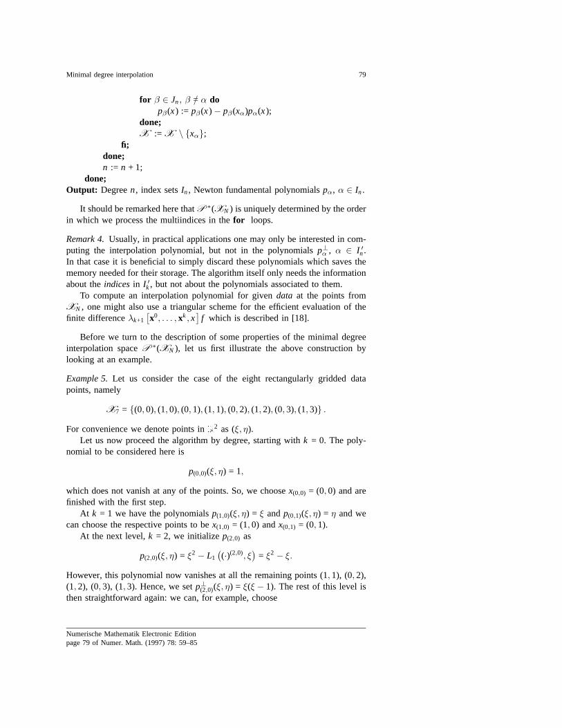
Before we turn to the description of some properties of the minimal degreeinterpolation spaceP ∗(XN ), let us first illustrate the above construction bylooking at an example.

Example 5.Let us consider the case of the eight rectangularly gridded datapoints, namely

X7 = {(0, 0), (1, 0), (0, 1), (1, 1), (0, 2), (1, 2), (0, 3), (1, 3)} .For convenience we denote points inR2 as (ξ, η).

Let us now proceed the algorithm by degree, starting withk = 0. The poly-nomial to be considered here is

p(0,0)(ξ, η) = 1,

which does not vanish at any of the points. So, we choosex(0,0) = (0, 0) and arefinished with the first step.

At k = 1 we have the polynomialsp(1,0)(ξ, η) = ξ andp(0,1)(ξ, η) = η and wecan choose the respective points to bex(1,0) = (1, 0) andx(0,1) = (0, 1).

At the next level,k = 2, we initializep(2,0) as

p(2,0)(ξ, η) = ξ2 − L1((·)(2,0), ξ

)= ξ2 − ξ.

However, this polynomial now vanishes at all the remaining points (1, 1), (0, 2),(1, 2), (0, 3), (1, 3). Hence, we setp⊥(2,0)(ξ, η) = ξ(ξ − 1). The rest of this level isthen straightforward again: we can, for example, choose


80 Th. Sauer

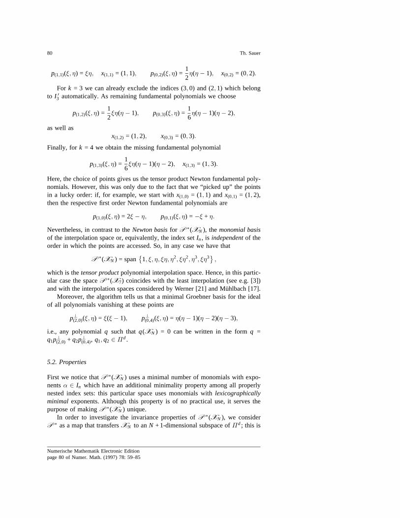
p(1,1)(ξ, η) = ξη, x(1,1) = (1, 1), p(0,2)(ξ, η) =12η(η − 1), x(0,2) = (0, 2).

For k = 3 we can already exclude the indices (3, 0) and (2, 1) which belongto I ′3 automatically. As remaining fundamental polynomials we choose

p(1,2)(ξ, η) =12ξη(η − 1), p(0,3)(ξ, η) =

16η(η − 1)(η − 2),

as well asx(1,2) = (1, 2), x(0,3) = (0, 3).

Finally, for k = 4 we obtain the missing fundamental polynomial

p(1,3)(ξ, η) =16ξη(η − 1)(η − 2), x(1,3) = (1, 3).

Here, the choice of points gives us the tensor product Newton fundamental poly-nomials. However, this was only due to the fact that we “picked up” the pointsin a lucky order: if, for example, we start withx(1,0) = (1, 1) andx(0,1) = (1, 2),then the respective first order Newton fundamental polynomials are

p(1,0)(ξ, η) = 2ξ − η, p(0,1)(ξ, η) = −ξ + η.

Nevertheless, in contrast to theNewton basisfor P ∗(XN ), the monomial basisof the interpolation space or, equivalently, the index setIn, is independentof theorder in which the points are accessed. So, in any case we have that

P ∗(XN ) = span{

1, ξ, η, ξη, η2, ξη2, η3, ξη3},

which is thetensor productpolynomial interpolation space. Hence, in this partic-ular case the spaceP ∗(X7) coincides with the least interpolation (see e.g. [3])and with the interpolation spaces considered by Werner [21] and Muhlbach [17].

Moreover, the algorithm tells us that a minimal Groebner basis for the idealof all polynomials vanishing at these points are

p⊥(2,0)(ξ, η) = ξ(ξ − 1), p⊥(0,4)(ξ, η) = η(η − 1)(η − 2)(η − 3),

i.e., any polynomialq such thatq(XN ) = 0 can be written in the formq =q1p⊥(2,0) + q2p⊥(0,4), q1, q2 ∈ Πd.

5.2. Properties

First we notice thatP ∗(XN ) uses a minimal number of monomials with expo-nentsα ∈ In which have an additional minimality property among all properlynested index sets: this particular space uses monomials withlexicographicallyminimal exponents. Although this property is of no practical use, it serves thepurpose of makingP ∗(XN ) unique.

In order to investigate the invariance properties ofP ∗(XN ), we considerP ∗ as a map that transfersXN to anN + 1-dimensional subspace ofΠd; this is



possible sinceP ∗ assigns auniquepolynomial subspace to each subset ofRd

consisting ofN + 1 elements by the construction from the preceding subsection.Let ϕ : Rd → R

d be some map, thenP ∗ is calledϕ-invariant if for any finitesubsetXN

P ∗ (ϕ(XN ))

= P ∗(XN ),

whereϕ(XN ) = {ϕ(x0), . . . , ϕ(xN )}.We will show that the construction rule forP ∗(XN ) implies that the space

generated this way is

1. scale invariant2. translation invariant

and thus closed under taking derivatives as well.Clearly, a minimal degree interpolation space is scale–invariant if it is

spanned by homogeneous polynomials – the (still homogeneous) polynomialspα(·/c) = c−|α|pα are obviously a basis for the minimal degree interpolationspace with respect tocXN with the same minimality properties as the originalone,XN . Since it is indeed spanned by homogeneous polynomials,P ∗(XN ) isscale–invariant, i.e.,

P ∗(XN ) = P ∗(cXN ), c ∈ R, c /= 0.

A little more effort has to be taken to prove the translation invariance ofP ∗(XN ), i.e.,

P ∗(XN ) = P ∗(XN − y), y ∈ Rd.

Obviously, a set of Newton fundamental polynomials with respect toXN − y isgiven by the polynomials

pα(· + y), α ∈ In,

and their span, sayP , is again a minimal degree interpolation space. On theother hand, we know that

P = span{(· + y)α : α ∈ In}.Since

(x + y)α =∑β≤α

(α

β

)xβyα−β =:

∑β≤α

cβxβ ,

we can apply Remark 1 to obtain that

P ∗(XN − y) = span{(x + y)α : α ∈ In} ⊂ span{xα : α ∈ In} = P ∗(XN ).

ReplacingXN by XN + y and theny by −y also yields the converse inclusion.HenceP ∗(XN ) is also translation–invariant. Together these two invariance prop-erties imply thatP ∗(XN ) is D–invariant, too, i.e., the space is closed under theoperation of taking derivatives.

It has been pointed out in [6] that least interpolation is not invariant underarbitrary rotations of the coordinate system. The same holds true forP ∗(XN ).Instead of dwelling on this in general, let us consider one example here whichnevertheless illuminates the phenomenon.


82 Th. Sauer

Example 6.Let the pointsx0, . . . , xN lie on on a line passing through the originand let us rotate them such that the origin remains fixed. Clearly, as long as theline which contains the points is not perpendicular to theξd–axis,P ∗(XN ) isalways a minimal degree interpolation space with respect to the rotated points.This is due to the lexicographical ordering which in this case always gives usthe polynomials 1, ξd, . . . , ξ

Nd as a basis forP ∗(XN ). However, if the the line

coincides with one coordinate axis, sayξk , then the projection to this coordinateaxis, spanned by 1, ξk , . . . , ξ

Nk , is the one and only minimal degree interpolation

space which uses a minimal number of monomials. Hence, in this case alsoP ∗(XN ) = span

{1, ξk , . . . , ξ

Nk

}. So,P ∗(XN ) is not rotation–invariant.

Least interpolation was described in (7) by a differential operator involvingthe leading terms of all polynomials which vanish in the interpolation points.It is interesting that something similar holds forP ∗(XN ), too, involving onlycertain partial derivatives. Indeed, if we define

I ′ = Nd0 \ In = I ′n ∪

{α ∈ Nd

0 : |α| > n}

then we can trivially reformulate the fact thatP ∗(XN ) is spanned by the mono-mials xα, α ∈ In, as

P ∗(XN ) =⋂α∈I ′

{p ∈ Πd :

∂|α|

xαp ≡ 0

}=⋂α∈I ′

kern Dα.

5.3. Numerical performance

In this section we finally lay out that Lagrange interpolation from the spaceP ∗(XN ) can be handled numerically in a very efficient way. In particular, forpolynomials in this space one can not only carry out the vector space operationsaddition/subtraction as well as multiplication by a real number withN operations(which is trivial), it is even possible to state a Horner scheme which evaluatespolynomials inP ∗(XN ) with the optimal number ofN nested additions andmultiplications. This in turn yields thatP ∗(XN ) is very suitable with respectto speed and numerical robustness, since a minimum of operations also reducesroundoff errors to the greatest possible extent.

In order to express this fact in greater detail, let us first recall the multivariateHorner scheme(see [18]) which evaluates a polynomial

p(x) =∑|α|≤n

cαxα, n ∈ N,

recursively by the nested multiplications

p(x) = ξ1(· · · ξ1(ξ1pn(x1) + pn−1(x1)) · · ·) + p0(x1),

wherex1 = (ξ2, . . . , ξd) and



Πd−1n−j 3 pj (x1) =

∑|α|≤n, α1=j

cαxα−j ·e1

, j = 0, . . . , n.

The same process, with respect toξ2 is then applied to each of the polynomialspj (x1) to be expanded into

pj (x1) = ξ2(· · · ξ2(ξ2pj ,n−j (x1,2) + pj ,n−j−1(x1,2)) · · ·) + pj ,0(x1,2),

j = 0, . . . , n,

where x1,2 = (ξ3, . . . , ξd), and so on. Following [18], we observe that in thisevaluation algorithm the coefficientscα, |α| ≤ n, are processed indescendinglexicographical order, i.e.,cα is accessed earlier thancβ iff α appears later thanβin the lexicographical ordering. In particular, every coefficient is accessed onlyonce in the evaluation process. Since in practical applications the coefficientsof a polynomial are in an array of the formc[0...N] , there is no need ofpermanently applying a function which transforms multiindices into the linearindex; conveniently the coefficients are arranged in a graded lexicographicalorder. Nevertheless, when using the above Horner scheme it suffices to provideonly a table which maps the lexicographical arrangement of the multiindices intothe linear ordering.

To derive the Horner scheme for polynomials inP ∗(XN ), we define

i1 = max{α1 : α ∈ Jn}and note that, by (28), the indices in the set

In(i1) ={α ∈ Nd−1

0 : (i1, α) ∈ In}

(29)

again satisfy

α ∈ In(i1) ⇒{β ∈ Nd−1

0 : β ≤ α}⊂ In(i1).

Applying (28) once more, we observe that together with (i1, α) we also have that(j , α) ∈ In, j = 0, . . . , i1, and that the respective setsIn(j ), defined according to(29), satisfy

α ∈ In(j ) ⇒{β ∈ Nd−1

0 : β ≤ α}⊂ In(j ), j = 0, . . . , i1.(30)

Hence, we can expandp ∈ P ∗(XN ), say

p(x) =∑α∈In

cαxα,

asp(x) = ξ1

(· · · ξ1(ξ1pi1(x1) + pi1−1(x1)) · · ·) + p0(x1).(31)

Noticing that the exponents in the (d − 1)-variate polynomialspj satisfy therespective version of (28) again, we can proceed recursively to evaluate thepolynomial. Note that this algorithm needs exactly as many additions and mul-tiplications as the polynomial has coefficients; thus, evaluation of a polynomialcan be done with 2N arithmetic operations.


84 Th. Sauer

Moreover, the polynomialpi1 has the form

pi1(x1) =∑

α∈In, α1=i1

cαxα−i1e1

and is evaluated first in the recursive process. By identical arguments as in [18] wetherefore obtain that the coefficients are processed in descending lexicographicalorder during the evaluation algorithm. Hence, we can again spare the conver-sion of multiindices into the linear indices0...N of the internal representationc[0...N] during the evaluation process and replace it by a conversion table.

These above features make the spaceP ∗(XN ) particularly handy for nu-merical purposes.

Nevertheless, one statement of warning may be in order here: all the methodsdeveloped in this paper require that it is possible to decidepreciselywhether apolynomial vanishes at a certain point or not. This usuallycannot be done infloating point arithmetics, where all the above statements and constructions areonly precise up to a certain threshold level. However, if one is interested in reallyexact interpolation at, say, rational points, then the above algorithm can be usedin connection with an infinite precision rationals library.

AcknowledgementsI want to thank Yuan Xu and Carl de Boor for a lot of stimulating discussionsand valuable comments. Also, I am very grateful to the referee for the exceptionally careful review,the helpful suggestions and the patience with my mistakes.

References

1. Boor, C. de (1994): Gauss elimination by segments and multivariate polynomial interpolation. In:Zahar, R.V.M. (ed) Approximation and Computation: A Festschrift in Honor of Walter Gautschi,pp. 87–96, Birkhauser

2. Boor, C. de (1995): A multivariate divided difference. In: Chui, C.K., Schumaker, L.L. (eds)Approximation Theory VIII, Vol. 1: Approximation and Interpolation, pp. 87–96, World ScientificPublishing Co.

3. Boor, C. de, Ron, A. (1990): On multivariate polynomial interpolation. Constr. Approx.6, 287–302

4. Boor, C. de, Ron, A. (1991): On polynomial ideals of finite codimension with applications tobox spline theory. J. Math. Anal. and Appl.158, 168–193

5. Boor, C. de, Ron, A. (1992): Computational aspects of polynomial interpolation in severalvariables. Math. Comp.58, 705–727

6. Boor, C. de, Ron, A. (1992): The least solution for the polynomial interpolation problem. Math.Z. 210, 347–378

7. Chung, K.C., Yao, T.H. (1977): On lattices admitting unique Lagrange interpolation. SIAM J.Num. Anal.14, 735–743

8. Ciarlet, P.G., Raviart, P.A. (1972): General Lagrange and Hermite interpolation inRn with

applications to finite element methods. Arch. Rational Mech. Anal.46, 178–1999. Gasca, M. (1990): Multivariate polynomial interpolation. In: Dahmen, W., Gasca, M., Micchelli,

C.A. (eds) Computation of Curves and Surfaces, pp. 215–236, Kluwer Academic Publishers10. Gasca, M., Maeztu, J.I. (1982): On Lagrange and Hermite interpolation inR

k . Numer. Math.39, 1–14

11. Kergin, P. (1980): A natural interpolation ofCK functions. J. Approx. Theory29, 278–29312. Kunz, K.S. (1957): Numerical Analysis. McGraw-Hill Book Company



13. Lorentz. G.G., Lorentz, R.A. (1986): Solvabiblity problems of bivariate interpolation. I. Constr.Approx. 2, 153–170

14. Lorentz, R.A. (1992): Multivariate Birkhoff Interpolation. Number 1516 in Lecture Notes inMathematics. Springer

15. Micchelli, C.A. (1980): A constructive approach to Kergin interpolation inRk : multivariateB–splines and Lagrange interpolation. Rocky Mountain J. Math.10, 485–497

16. Micchelli, C.A. (1979): On a numerically efficient method of computing multivariate B-splines.In: Schempp, W., Zeller, K. (eds) Multivariate Approximation Theory, pp. 211–248, Birkhauser,Basel

17. Muhlbach, G. (1988): On multivariate interpolation by generalized polynomials on subsets ofgrids. Computing40, 201–215

18. Sauer, Th. (1995): Computational aspects of multivariate polynomial interpolation. Advances inComp. Math.3, 219–238

19. Sauer, Th., Xu, Y. (1995): On multivariate Hermite interpolation. Advances in Comp. Math.4, 207–259

20. Sauer, Th., Xu, Y. (1995) On multivariate Lagrange interpolation. Math. Comp.64, 1147–117021. Werner, H. (1980): Remarks on Newton type multivariate interpolation for subsets of grids.

Computing25, 181–191

This article was processed by the author using the LaTEX style file pljour1m from Springer-Verlag.


polynomial interpolation of minimal degree

Documents