pollutant load reduction model (plrm) - casqa defining hydrology and hydrologic source controls...
TRANSCRIPT
Pollutant Load Reduction Model(PLRM)
U s e r ' s M a n u a lU s e r ' s M a n u a l
December 2009

Terms and Conditions for Use
The software product is provided on an "as-is" basis. The members of the PLRM Development
Team (United States Government, State of California, State of Nevada, Northwest Hydraulic
Consultants Inc.; Geosyntec Consultants, Inc.; and 2NDNATURE, LLC) make no
representations or warranties of any kind, and specifically disclaim, without limitation, any
implied warranties of title, merchantability, applicability, fitness for a particular purpose, and
non-infringement. Although care has been used in preparing the software product, the PLRM
Development Team members disclaim all liability for its accuracy or completeness, and the user
shall be solely responsible for the selection, use, efficiency and suitability of the software
product. Members of the PLRM Development Team and their agencies, officials,
representatives, employees and subcontractors shall not be liable for lost profits or any special,
incidental, or consequential damages arising out of or in connection with use of PLRM
regardless of cause, including negligence. PLRM Development Team members shall have no
liability to users for the infringement of proprietary rights by the software product or any portion
thereof. Any person who uses this product does so at their sole risk and without liability to
members of the PLRM Development Team. By using this product you voluntarily agree to these
terms and conditions.
Foreword and Acknowledgements
The Pollutant Load Reduction Model is part of a multi-stakeholder effort to provide technical
tools for project planners, funders, implementers, and regulators to work collaboratively to
minimize the deleterious effects of urban storm water on the remarkable clarity of Lake Tahoe, a
keystone in the ecological and economic health of the Lake Tahoe Basin. This product would
not be possible without the generous participation of several Basin regulatory and project
implementing entities. This specific product is authorized pursuant to Section 234 of the Water
Resources Development Act of 1996 (PL 104-303) which provides for coordinated interagency
efforts in the pursuit of water quality and watershed planning.
This product was funded by:
Support and in-kind services were provided by:
This product was prepared by:
PLRM User’s Manual i December 2009
TABLE OF CONTENTS
1.0 INTRODUCTION AND OVERVIEW ................................................................................. 1
1.1 INTENDED USE OF THE PLRM ................................................................................................ 1
1.2 PLRM DOCUMENTATION ....................................................................................................... 2
1.3 USER’S MANUAL CONTENT ................................................................................................... 3
1.4 MODELING APPROACH AND CAPABILITIES............................................................................. 4
1.5 INSTALLING AND RUNNING THE PROGRAM ............................................................................ 7
2.0 QUICK START GUIDE......................................................................................................... 9
2.1 STARTING A NEW PROJECT AND SCENARIO.......................................................................... 10
2.2 DEVELOPING A SCHEMATIC ................................................................................................. 14
2.3 ENTERING CATCHMENT DATA ............................................................................................. 16
2.4 LAND USE CONDITIONS AND POLLUTANT SOURCE CONTROLS ............................................ 21
2.5 HYDROLOGY AND HYDROLOGIC SOURCE CONTROLS .......................................................... 24
2.6 STORM WATER TREATMENT ................................................................................................ 27
2.7 RUNNING THE MODEL AND VIEWING RESULTS .................................................................... 30
3.0 WORKING WITH PROJECTS AND SCENARIOS ........................................................ 34
3.1 PROJECT EDITOR .................................................................................................................. 35
3.2 SCENARIO EDITOR................................................................................................................ 37
3.3 MANAGING PROJECTS AND SCENARIOS ON YOUR COMPUTER ............................................. 39
4.0 DEVELOPING A SCHEMATIC ........................................................................................ 41
5.0 ENTERING CATCHMENT DATA ................................................................................... 44
5.1 PHYSICAL ATTRIBUTES ........................................................................................................ 45
5.2 LAND USES .......................................................................................................................... 46
5.3 SOILS ................................................................................................................................... 48
6.0 DEFINING LAND USE CONDITIONS AND POLLUTANT SOURCE CONTROLS 50
6.1 ROAD METHODOLOGY ......................................................................................................... 51
6.1.1 Road Risk Categories ................................................................................................... 52
6.1.2 Road Conditions........................................................................................................... 55
6.2 PARCEL METHODOLOGY ...................................................................................................... 68
7.0 DEFINING HYDROLOGY AND HYDROLOGIC SOURCE CONTROLS ................. 71
7.1 DRAINAGE CONDITIONS ....................................................................................................... 73
7.2 HYDROLOGIC PROPERTIES OF LAND USES ........................................................................... 75
7.3 HYDROLOGIC PROPERTIES OF HSC FACILITIES .................................................................... 80
7.3.1 Infiltration Facility Editor ........................................................................................... 81
7.3.2 Pervious Dispersion Area Editor ................................................................................. 82
8.0 DEFINING STORM WATER TREATMENT FACILITIES AND OBJECTS ............. 84
8.1 DRY BASIN ........................................................................................................................... 86
8.2 INFILTRATION BASIN ............................................................................................................ 90
PLRM User’s Manual ii December 2009
8.3 WET BASIN .......................................................................................................................... 94
8.4 BED FILTER .......................................................................................................................... 98
8.5 CARTRIDGE FILTER ............................................................................................................ 102
8.6 TREATMENT VAULT OR USER-DEFINED FLOW BASED SWT .............................................. 104
8.7 OUTFALLS, JUNCTIONS, AND FLOW DIVIDERS.................................................................... 106
9.0 RUNNING THE MODEL AND VIEWING RESULTS ................................................. 109
9.1 SCENARIO REPORT ............................................................................................................. 110
9.2 SCENARIO COMPARISON REPORT ....................................................................................... 114
10.0 PARAMETER GUIDANCE ............................................................................................ 116
10.1 DEFAULT PARAMETERS.................................................................................................... 117
10.2 INPUT PARAMETERS ......................................................................................................... 118
11.0 PLRM DATABASE OVERVIEW .................................................................................. 135
12.0 NOTES ON PLRM MODELING.................................................................................... 147
12.1 LIMITATIONS AND STRUCTURE OF VERSION 1 .................................................................. 147
12.2 DEFINITIONS OF TERMS .................................................................................................... 151
PLRM User’s Manual iii December 2009
List of Figures
FIGURE 1.1 – MODELING APPROACH .................................................................................... 5
FIGURE 2.1 – PLRM ICON .......................................................................................................... 9
FIGURE 2.2 – STARTING THE PLRM ...................................................................................... 10
FIGURE 2.3 – PROJECT EDITOR.............................................................................................. 11
FIGURE 2.4 – PROJECT AND SCENARIO MANAGER ......................................................... 12
FIGURE 2.5 – SCENARIO EDITOR .......................................................................................... 13
FIGURE 2.6 – SCHEMATIC WINDOW AND FUNCTIONS ................................................... 15
FIGURE 2.7 – QUICK START EXAMPLE ELEMENTS .......................................................... 16
FIGURE 2.8 – CATCHMENT PROPERTIES EDITOR ............................................................. 17
FIGURE 2.9 – LAND USE EDITOR ........................................................................................... 19
FIGURE 2.10 – SOILS EDITOR ................................................................................................. 20
FIGURE 2.11 – LAND USE CONDITIONS EDITOR ............................................................... 21 FIGURE 2.12 – ROAD CONDITIONS EDITOR ........................................................................ 23
FIGURE 2.13 – DRAINAGE CONDITIONS EDITOR (ROAD METHODOLOGY) ............... 25
FIGURE 2.14 – DRAINAGE CONDITIONS EDITOR (PARCEL METHODOLOGY) ........... 26
FIGURE 2.15 – DRY BASIN EDITOR ....................................................................................... 28
FIGURE 2.16 – DRY BASIN REPRESENTATION IN PLRM .................................................. 29
FIGURE 2.17 – RECOMMENDED RANGE REPORT .............................................................. 30
FIGURE 2.18 – SCENARIO REPORT ........................................................................................ 31
FIGURE 2.19 – SCENARIO COMPARISON REPORT............................................................. 32
FIGURE 3.1 – PROJECT AND SCENARIO EDITOR ............................................................... 34
FIGURE 3.2 – PROJECT EDITOR.............................................................................................. 36
FIGURE 3.3 – SCENARIO EDITOR .......................................................................................... 38
FIGURE 3.4 – FINDING PROJECT AND SCENARIO FOLDERS ON YOUR COMPUTER 40
FIGURE 4.1 – SCHEMATIC WINDOW AND FUNCTIONS ................................................... 41
FIGURE 5.1 – CATCHMENT PROPERTIES EDITOR ............................................................. 44
FIGURE 5.2 – LAND USE EDITOR ........................................................................................... 47
FIGURE 5.3 – SOILS EDITOR ................................................................................................... 48
FIGURE 6.1 – LAND USE CONDITIONS EDITOR: ROAD METHODOLOGY .................... 50
FIGURE 6.2 – EXAMPLE OF DEFAULT ROAD RISK LAYER ............................................. 53
FIGURE 6.3 – ROAD CONDITIONS EDITOR .......................................................................... 55
FIGURE 6.4 – ROAD SHOULDER CONDITION DECISION PROCESS ............................... 58
FIGURE 6.6 – LAND USE CONDITIONS EDITOR: PARCEL METHODOLOGY ................ 68
FIGURE 7.1 – DRAINAGE CONDITIONS EDITOR (ROAD METHODOLOGY) ................. 71
FIGURE 7.2 – ENTERING HYDROLOGIC PROPERTIES FOR A DRAINAGE AREA ........ 76
FIGURE 7.3 – SIMPLIFIED IMPERVIOUS AREA CONNECTIVITY DEPICTION .............. 77
FIGURE 7.4 – ACCESS TO HSC FACILITY EDITORS ........................................................... 80
FIGURE 7.5 – INFILTRATION FACILITY EDITOR ............................................................... 81
FIGURE 7.6 – PERVIOUS DISPERSION AREA EDITOR ....................................................... 82
FIGURE 8.1 – DRY BASIN EDITOR ......................................................................................... 86
FIGURE 8.2 – DRY BASIN REPRESENTATION IN PLRM .................................................... 88
FIGURE 8.3 – DRY BASIN VOLUME-DISCHARGE CURVE EDITOR ................................ 89
FIGURE 8.4 – INFILTRATION BASIN EDITOR ...................................................................... 90
FIGURE 8.5 – INFILTRATION BASIN REPRESENTATION IN PLRM ................................ 91
FIGURE 8.6 – INFILTRATION BASIN VOLUME-DISCHARGE CURVE EDITOR ............. 93
PLRM User’s Manual iv December 2009
FIGURE 8.7 – WET BASIN EDITOR ......................................................................................... 94
FIGURE 8.8 – WET BASIN REPRESENTATION IN PLRM ................................................... 96
FIGURE 8.9 – WET BASIN VOLUME-DISCHARGE CURVE EDITOR ................................ 97
FIGURE 8.10 – BED FILTER EDITOR ...................................................................................... 98
FIGURE 8.11 – BED FILTER REPRESENTATION IN PLRM................................................. 99
FIGURE 8.12 – BED FILTER VOLUME-DISCHARGE CURVE EDITOR ........................... 101
FIGURE 8.13 – CARTRIDGE FILTER EDITOR ..................................................................... 102
FIGURE 8.14 – CARTRIDGE FILTER REPRESENTATION IN PLRM ................................ 103
FIGURE 8.15 – TREATMENT VAULT EDITOR .................................................................... 104
FIGURE 8.16 – TREATMENT VAULT REPRESENTATION IN PLRM .............................. 105
FIGURE 8.17 – OUTFALL EDITOR ........................................................................................ 106
FIGURE 8.18 – JUNCTION EDITOR ....................................................................................... 107
FIGURE 8.19 – FLOW DIVIDER EDITOR .............................................................................. 108
FIGURE 9.1 – RECOMMENDED RANGE REPORT .............................................................. 109
FIGURE 9.2 – SCENARIO REPORT ........................................................................................ 111
FIGURE 9.3 – SCENARIO COMPARISON REPORT............................................................. 114
FIGURE 11.1 – SIMPLIFIED IMPERVIOUS AREA CONNECTIVITY DEPICTION .......... 124
FIGURE 11.1 – PLRM DATABASE AND PROGRAM STRUCTURE .................................. 136
List of Tables
TABLE 1.1 – DESCRIPTION OF PLRM DOCUMENTATION.................................................. 2
TABLE 6.1 – CRITERIA FOR DEFAULT ROAD RISK GIS LAYER ..................................... 54
TABLE 6.2 – ROAD ABRASIVE APPLICATION STRATEGIES ........................................... 56
TABLE 6.3 – ROAD SHOULDER CONDITIONS INPUT ........................................................ 58
TABLE 6.4 – SWEEPER TYPE .................................................................................................. 66
TABLE 6.5 – PARCEL CRCS WITH AND WITHOUT PSCS .................................................. 70
TABLE 7.1 – DEFAULT PERCENT DCIA VALUES ............................................................... 78
TABLE 10.1 – SENSITIVE DEFAULT PARAMETERS WITHIN PLRM DATABASE ....... 117
TABLE 10.2 – SENSITIVE INPUT PARAMETERS WITHIN PLRM INTERFACE ............. 119
PLRM User’s Manual v December 2009
List of Abbreviations
BMP – Best Management Practice
CEC – Characteristic Effluent Concentration
CICU – Commercial, Institutional, Communications, Utilities
CRC – Characteristic Runoff Concentration
DIN – Dissolved Inorganic Nitrogen
FSP – Fine Sediment Particles (less than 16 microns)
GIS – Geographic Information System
GUI – Graphical User Interface
HSC – Hydrologic Source Control
HSG – Hydrologic Soil Group
KML – Keyhole Markup Language
Ksat – Saturated Hydraulic Conductivity
PLRM – Pollutant Load Reduction Model
PSC – Pollutant Source Controls
SRP – Soluble Reactive Phosphorus
SWMM5 – Storm Water Management Model version 5
SWT – Storm Water Treatment
TMDL – Total Maximum Daily Load
TN – Total Nitrogen
TP – Total Phosphorus
TSS – Total Suspended Sediment
XML – eXtensible Markup Language
XSLT – eXtensible Stylesheet Language Transformations
PLRM User’s Manual 1 December 2009
1.0 Introduction and Overview
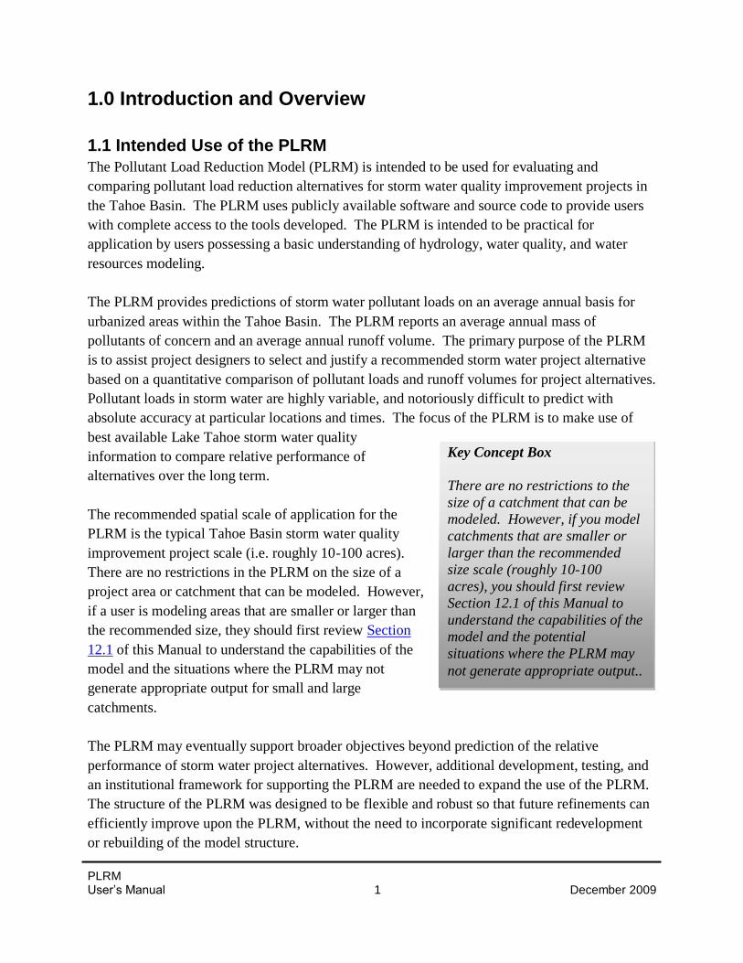
1.1 Intended Use of the PLRM
The Pollutant Load Reduction Model (PLRM) is intended to be used for evaluating and
comparing pollutant load reduction alternatives for storm water quality improvement projects in
the Tahoe Basin. The PLRM uses publicly available software and source code to provide users
with complete access to the tools developed. The PLRM is intended to be practical for
application by users possessing a basic understanding of hydrology, water quality, and water
resources modeling.
The PLRM provides predictions of storm water pollutant loads on an average annual basis for
urbanized areas within the Tahoe Basin. The PLRM reports an average annual mass of
pollutants of concern and an average annual runoff volume. The primary purpose of the PLRM
is to assist project designers to select and justify a recommended storm water project alternative
based on a quantitative comparison of pollutant loads and runoff volumes for project alternatives.
Pollutant loads in storm water are highly variable, and notoriously difficult to predict with
absolute accuracy at particular locations and times. The focus of the PLRM is to make use of
best available Lake Tahoe storm water quality
information to compare relative performance of
alternatives over the long term.
The recommended spatial scale of application for the
PLRM is the typical Tahoe Basin storm water quality
improvement project scale (i.e. roughly 10-100 acres).
There are no restrictions in the PLRM on the size of a
project area or catchment that can be modeled. However,
if a user is modeling areas that are smaller or larger than
the recommended size, they should first review Section
12.1 of this Manual to understand the capabilities of the
model and the situations where the PLRM may not
generate appropriate output for small and large
catchments.
The PLRM may eventually support broader objectives beyond prediction of the relative
performance of storm water project alternatives. However, additional development, testing, and
an institutional framework for supporting the PLRM are needed to expand the use of the PLRM.
The structure of the PLRM was designed to be flexible and robust so that future refinements can
efficiently improve upon the PLRM, without the need to incorporate significant redevelopment
or rebuilding of the model structure.
Key Concept Box
There are no restrictions to the
size of a catchment that can be
modeled. However, if you model
catchments that are smaller or
larger than the recommended
size scale (roughly 10-100
acres), you should first review
Section 12.1 of this Manual to
understand the capabilities of the
model and the potential
situations where the PLRM may
not generate appropriate output..
PLRM User’s Manual 2 December 2009
The PLRM is not intended to predict pollutant loads in non-
urbanized settings in the Tahoe Basin. The PLRM should
not be used to size facilities and conveyances for flood
protection. The PLRM will not replace tools and models
recommended by local and regional hydrology guidelines
or codes for flood protection. Finally, the model will not
explicitly evaluate the effects of hydrologic modification
on downstream channel erosion and associated sediment
loads.
1.2 PLRM Documentation
This User’s Manual is one part of the documentation developed for the PLRM. Table 1.1 lists
three documents that are available to assist users in applying and understanding the PLRM.
Table 1.1 – Description of PLRM Documentation
Documentation Description
User's Manual
The manual is the primary document describing how to use the PLRM.
The manual provides information that is directly applicable for setting
up and performing basic PLRM simulations.
Applications Guide
The guide provides simple example applications of the PLRM. The
example applications walk the user through the basic steps of
developing a PLRM simulation and interpreting results.
Model Development
Document
The document supplements the User's Manual by providing the
interested reader with more background on the PLRM program
structure; development of data sets supporting the PLRM; and technical
algorithms used to develop data sets as well as inform computational
methods. Although the information in this document will not generally
be needed to perform basic simulations, it provides important
background on the fundamental model structure and supports a more
in-depth understanding of model computations and a baseline for future
model development.
Key Concept Box
The PLRM should not be used to
size facilities and conveyances
for flood protection. The PLRM
will not replace tools and models
recommended by local and
regional hydrology guidelines or
codes for flood protection.
PLRM User’s Manual 3 December 2009
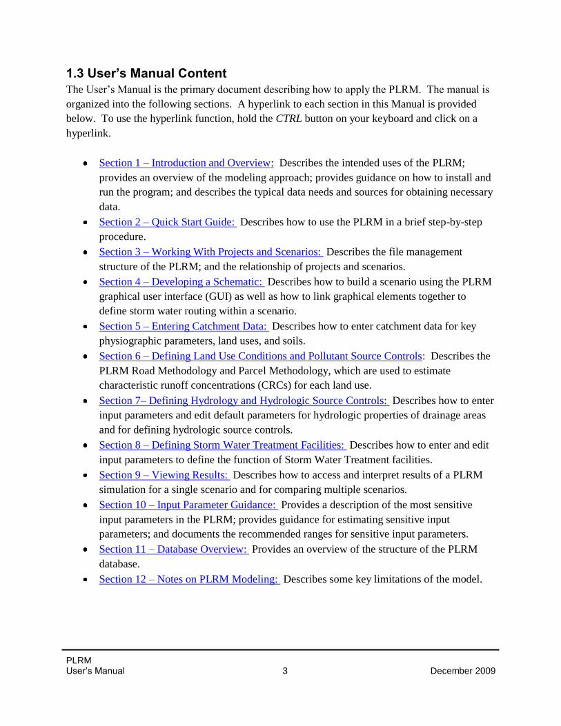
1.3 User’s Manual Content
The User’s Manual is the primary document describing how to apply the PLRM. The manual is
organized into the following sections. A hyperlink to each section in this Manual is provided
below. To use the hyperlink function, hold the CTRL button on your keyboard and click on a
hyperlink.
Section 1 – Introduction and Overview: Describes the intended uses of the PLRM;
provides an overview of the modeling approach; provides guidance on how to install and
run the program; and describes the typical data needs and sources for obtaining necessary
data.
Section 2 – Quick Start Guide: Describes how to use the PLRM in a brief step-by-step
procedure.
Section 3 – Working With Projects and Scenarios: Describes the file management
structure of the PLRM; and the relationship of projects and scenarios.
Section 4 – Developing a Schematic: Describes how to build a scenario using the PLRM
graphical user interface (GUI) as well as how to link graphical elements together to
define storm water routing within a scenario.
Section 5 – Entering Catchment Data: Describes how to enter catchment data for key
physiographic parameters, land uses, and soils.
Section 6 – Defining Land Use Conditions and Pollutant Source Controls: Describes the
PLRM Road Methodology and Parcel Methodology, which are used to estimate
characteristic runoff concentrations (CRCs) for each land use.
Section 7– Defining Hydrology and Hydrologic Source Controls: Describes how to enter
input parameters and edit default parameters for hydrologic properties of drainage areas
and for defining hydrologic source controls.
Section 8 – Defining Storm Water Treatment Facilities: Describes how to enter and edit
input parameters to define the function of Storm Water Treatment facilities.
Section 9 – Viewing Results: Describes how to access and interpret results of a PLRM
simulation for a single scenario and for comparing multiple scenarios.
Section 10 – Input Parameter Guidance: Provides a description of the most sensitive
input parameters in the PLRM; provides guidance for estimating sensitive input
parameters; and documents the recommended ranges for sensitive input parameters.
Section 11 – Database Overview: Provides an overview of the structure of the PLRM
database.
Section 12 – Notes on PLRM Modeling: Describes some key limitations of the model.
PLRM User’s Manual 4 December 2009
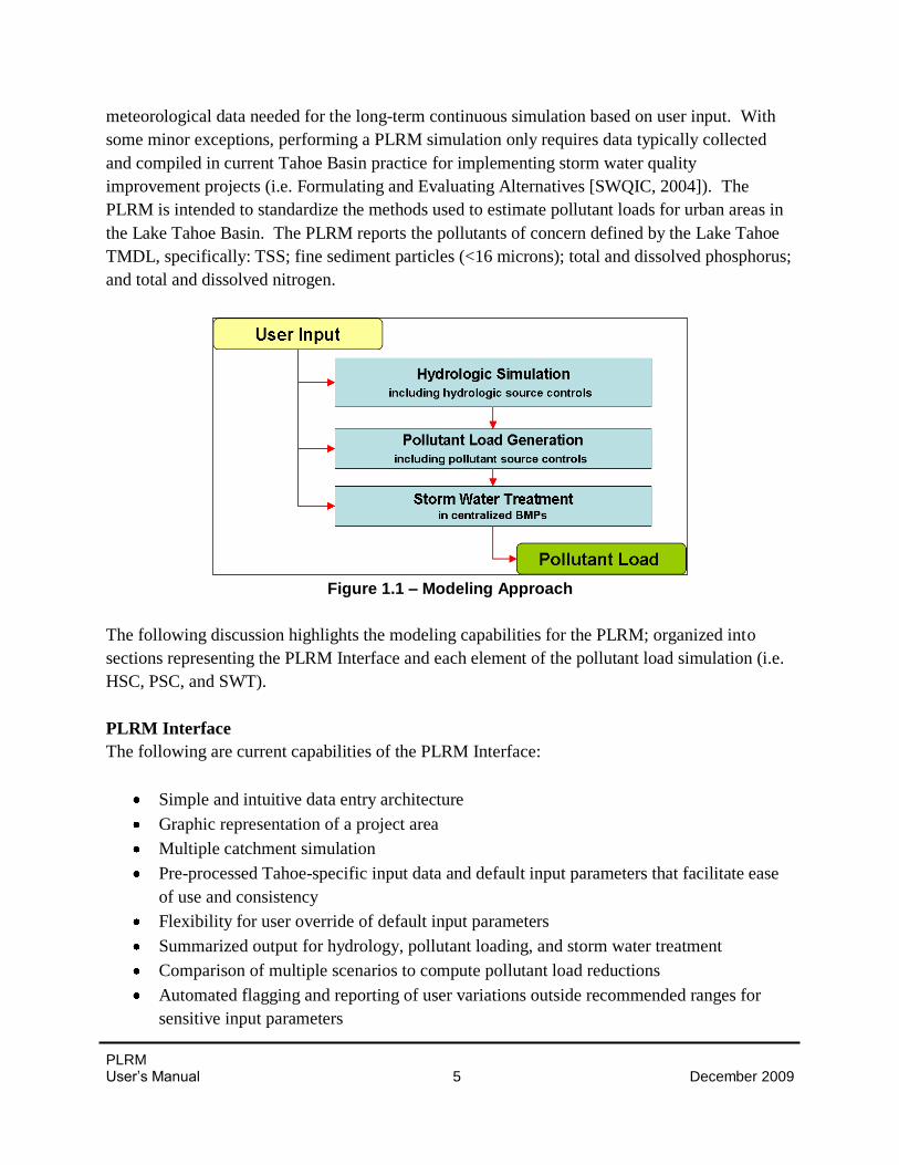
1.4 Modeling Approach and Capabilities
Figure 1.1 illustrates the three elements used for simulating pollutant loads in the PLRM: 1)
hydrology and hydrologic source controls (HSC), 2) pollutant load generation and pollutant
source controls (PSC), and 3) storm water treatment (SWT). User input is required for each
element, and the results derived from each element are used in subsequent elements. Computed
pollutant loads represent the combined effectiveness of the three major elements. A detailed
rationale for the modeling approach is discussed in the report: Methodology to Estimate
Pollutant Load Reductions (nhc and Geosytnec, 2006). The definition of each element is as
follows:
Hydrology and Hydrologic Source Controls (HSCs)
Hydrology is reported as average annual runoff volumes from long-term continuous
simulations of precipitation and runoff. Continuous hydrologic simulations include many
time steps over a specified period of time; including many hydrologic events and
intervening dry periods (rather than a single storm) to represent the full range of
hydrologic conditions during the period of time simulated.
HSCs reduce runoff volumes and minimize the concentration of storm water runoff
through distributed runoff interception, infiltration, and disconnection of impervious
surfaces. HSCs primarily function to increase infiltration, which routes precipitation or
surface runoff to groundwater.
Pollutant Generation and Pollutant Source Controls (PSCs)
Pollutant generation focuses on estimating the total pollutant load from a drainage
catchment based on the characteristics of the catchment, in particular the land uses with
the catchment and the condition of the land uses. The product of storm water volume and
storm water pollutant concentration is the pollutant load generated from the catchment.
PSCs reduce the generation of pollutants of concern at their sources by inhibiting or
reducing mobilization and transport of pollutants with storm water.
Storm Water Treatment (SWT)
SWT removes pollutants of concern after they have entered concentrated storm water
runoff flow paths. This might include treatment of flows infiltrated to groundwater as
well as those discharged to surface waters.
The PLRM streamlines and automates many of the data inputs required to setup and execute a
simulation. The PLRM is intended to minimize the burden on the end user for data collection
and data compilation. For example, the PLRM automatically generates location-specific
PLRM User’s Manual 5 December 2009
meteorological data needed for the long-term continuous simulation based on user input. With
some minor exceptions, performing a PLRM simulation only requires data typically collected
and compiled in current Tahoe Basin practice for implementing storm water quality
improvement projects (i.e. Formulating and Evaluating Alternatives [SWQIC, 2004]). The
PLRM is intended to standardize the methods used to estimate pollutant loads for urban areas in
the Lake Tahoe Basin. The PLRM reports the pollutants of concern defined by the Lake Tahoe
TMDL, specifically: TSS; fine sediment particles (<16 microns); total and dissolved phosphorus;
and total and dissolved nitrogen.
Figure 1.1 – Modeling Approach
The following discussion highlights the modeling capabilities for the PLRM; organized into
sections representing the PLRM Interface and each element of the pollutant load simulation (i.e.
HSC, PSC, and SWT).
PLRM Interface
The following are current capabilities of the PLRM Interface:
Simple and intuitive data entry architecture
Graphic representation of a project area
Multiple catchment simulation
Pre-processed Tahoe-specific input data and default input parameters that facilitate ease
of use and consistency
Flexibility for user override of default input parameters
Summarized output for hydrology, pollutant loading, and storm water treatment
Comparison of multiple scenarios to compute pollutant load reductions
Automated flagging and reporting of user variations outside recommended ranges for
sensitive input parameters
PLRM User’s Manual 6 December 2009
Hydrology and Hydrologic Source Controls (HSC)
Hydrologic simulations in the PLRM include the following capabilities:
Snowfall and snowmelt
Effects of directly and indirectly connected impervious area, including routing directly
connected areas to pervious areas
Private property BMP implementation
Infiltration and evapotranspiration, including accounting and reporting of volumes
For the hydrologic computations in the PLRM, pre-processed input data sets and default input
parameters are provided to represent Tahoe Basin conditions. Pre-load input data sets include:
Long-term meteorological data sets of precipitation and temperature at hourly intervals
Snowmelt and snow management parameters
Evapotranspiration parameters
Hydrologic properties of soil from the Tahoe Basin Soil Survey (NRCS, 2006)
Pollutant Generation and Pollutant Source Control (PSC)
Pollutant generation in the PLRM is based on the product of average annual runoff and land use
based characteristic runoff concentrations (CRCs).
Two separate methods are used to represent the implementation of PSCs, which can reduce the
CRCs for 1) public right-of-ways (Road Methodology), and on 2) predominantly private land
uses (Parcel Methodology). Capabilities for simulating pollutant generation and PSC
implementation in the PLRM include:
Road Methodology – a standardized approach that integrates physiographic
characteristics, pollutant source control efforts, and pollutant recovery to predict the
likely road condition and associated CRCs
Parcel Methodology - a simple method to estimate improvements in CRCs from private
property BMP implementation consistent with current regulations
Storm Water Treatment (SWT)
The reduction in pollutant loading achieved by a SWT facility depends on the portion of runoff
treated and the extent of treatment achieved. The modeling approach calculates the percentage
of runoff captured by the SWT from user entered design information and long-term simulations
of hydrology. Runoff captured is assumed treated to a characteristic effluent concentration
(CEC). Runoff that is bypassed is assumed to equal influent concentration. Current capabilities
for SWT in the PLRM include:
PLRM User’s Manual 7 December 2009
Representation of volume based and flow based SWT facilities based on key design
criteria (e.g., water quality storage, drain time, water quality flow rate, infiltration rate,
etc.)
Representation of treatment trains
Pre-loaded defaults for CECs based on Tahoe Basin data sets supplemented by data from
the International BMP Database
Flexibility for user specified CECs to represent advanced or innovative treatment
1.5 Installing and Running the Program
Installation Procedure
1. To obtain the PLRM setup program, download the PLRM_Setup.zip file from the TIIMS
website: http://www.tiims.org/TIIMS-Sub-Sites/PLRM.aspx
2. After downloading the zip file, extract the contents to a folder on your computer.
3. In the folder, run the setup program PLRM_SetUp.exe from within the folder Install
PLRM.
4. Follow the instructions on the screen to install the
PLRM.
5. If you have Microsoft Access 2007 on your
computer skip this step. If you do not have
Microsoft Access 2007 on your computer, or are
unsure, you need to complete the following for the
PLRM to run on your computer:
a. After extracting the content from the
PLRM_Setup.zip file to your computer,
run the setup program AccessRuntime.exe
from within the folder Install Access
Runtime.
b. Follow the instructions on the screen to
install the free software: Microsoft Access
Runtime 2007.
The setup program will automatically create a program group called PLRM. The program group
will be listed under the Programs menu, which is under the Start menu. The PLRM icon will be
contained within the PLRM program group. The PLRM executable can be found in the directory
C:\Program Files\PLRM\Engine. Note that if you have administrative access limitations on your
computer, you should ask your computer administrator to give you “write access” to the
directory C:\Program Files\PLRM on your computer when your administrator installs the PLRM.
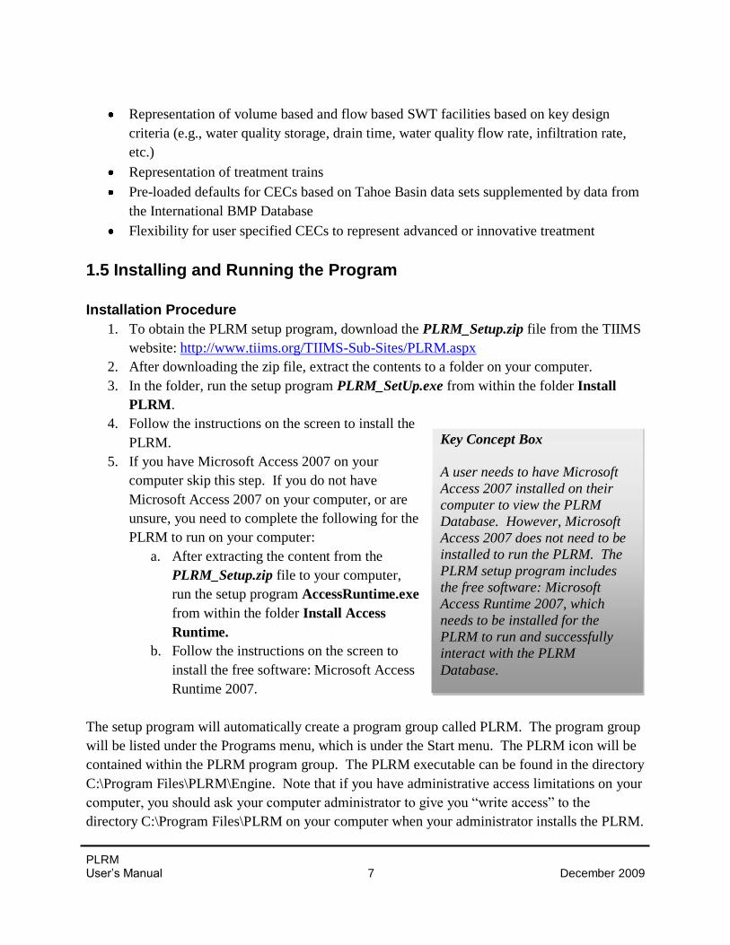
Key Concept Box
A user needs to have Microsoft
Access 2007 installed on their
computer to view the PLRM
Database. However, Microsoft
Access 2007 does not need to be
installed to run the PLRM. The
PLRM setup program includes
the free software: Microsoft
Access Runtime 2007, which
needs to be installed for the
PLRM to run and successfully
interact with the PLRM
Database.
PLRM User’s Manual 8 December 2009
Having write access to the C:\Program Files\PLRM will allow you to manage files better because
certain file management functions are have not been developed into PLRM Version 1 – see
Section 3.3.
Hardware Requirements
This version of the PLRM will run on a computer that has the following:
Intel Based PC or compatible machine with Pentium processor or higher (a Pentium III or
highly is recommended).
A hard disk with at least 1 gigabyte of free space.
A minimum of 256 megabytes of RAM, however additional RAM is recommended.
Windows XP (Service Pack III or newer).
Windows Vista with User Account Control turned off.
As of December 2009, PLRM has not been tested on Windows 7.
Uninstall Procedure
The PLRM setup program automatically registers the software with the Windows operating
system. The software can be uninstalled by clicking on the uninstall icon in the PLRM program
group under the Start menu, or by navigating to Add/Remove programs on the Control Panel.
PLRM User’s Manual 9 December 2009
2.0 Quick Start Guide This Quick Start Guide provides basic information on how to enter required information to
successfully build a PLRM simulation and run the program. This section does not provide any
guidelines regarding how to estimate Input Parameters or how the input forms influence
computations and results. Sections 3 through 11 of this User’s Manual should be reviewed to
gain a thorough understanding of the program, the Input Parameters required by the program,
and the guidelines for estimating Input Parameters.
To Start the PLRM:
When you run the PLRM setup program, you automatically get a new program group called
PLRM and associated program icon. The PLRM should appear in the start menu under
Programs. The setup program will also give you the option to create a shortcut on your desktop.
If you decide to create a shortcut, the icon on your desktop will look like Figure 2.1.
PLRM v1.0
Figure 2.1 – PLRM Icon
From your desktop, double-click on the PLRM icon. If you did not create a PLRM icon on your
desktop, go to the Start menu and select Programs, then select PLRM.
When you first start the PLRM you will see the Project and Scenario Manager as shown in
Figure 2.2. The PLRM Schematic Window will be visible in the background but will not be
accessible to you at this point.
PLRM User’s Manual 10 December 2009
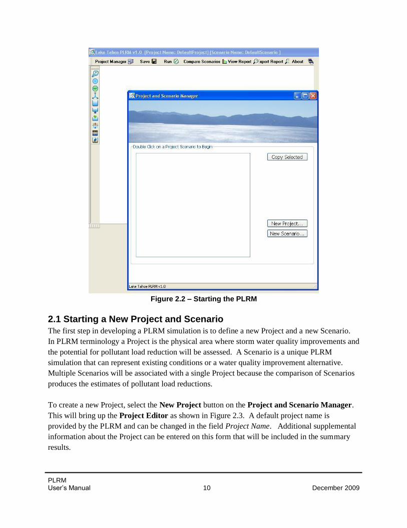
Figure 2.2 – Starting the PLRM
2.1 Starting a New Project and Scenario
The first step in developing a PLRM simulation is to define a new Project and a new Scenario.
In PLRM terminology a Project is the physical area where storm water quality improvements and
the potential for pollutant load reduction will be assessed. A Scenario is a unique PLRM
simulation that can represent existing conditions or a water quality improvement alternative.
Multiple Scenarios will be associated with a single Project because the comparison of Scenarios
produces the estimates of pollutant load reductions.
To create a new Project, select the New Project button on the Project and Scenario Manager.
This will bring up the Project Editor as shown in Figure 2.3. A default project name is
provided by the PLRM and can be changed in the field Project Name. Additional supplemental
information about the Project can be entered on this form that will be included in the summary
results.
PLRM User’s Manual 11 December 2009
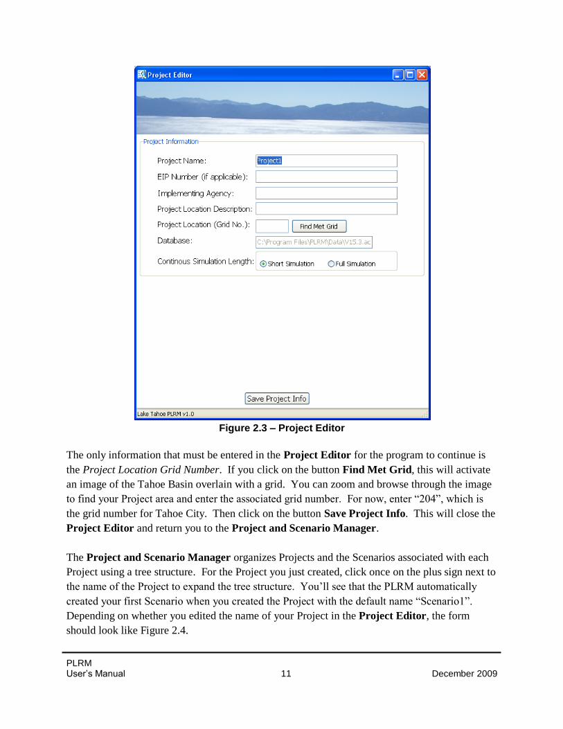
Figure 2.3 – Project Editor
The only information that must be entered in the Project Editor for the program to continue is
the Project Location Grid Number. If you click on the button Find Met Grid, this will activate
an image of the Tahoe Basin overlain with a grid. You can zoom and browse through the image
to find your Project area and enter the associated grid number. For now, enter “204”, which is
the grid number for Tahoe City. Then click on the button Save Project Info. This will close the
Project Editor and return you to the Project and Scenario Manager.
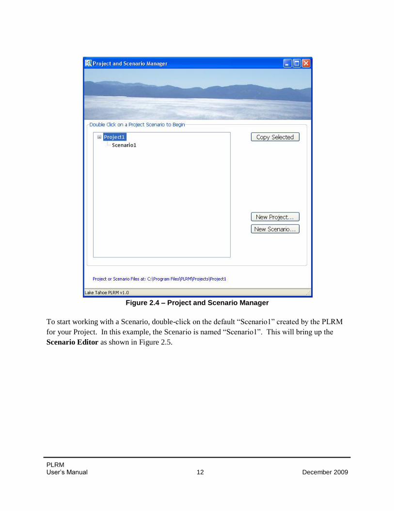
The Project and Scenario Manager organizes Projects and the Scenarios associated with each
Project using a tree structure. For the Project you just created, click once on the plus sign next to
the name of the Project to expand the tree structure. You’ll see that the PLRM automatically
created your first Scenario when you created the Project with the default name “Scenario1”.
Depending on whether you edited the name of your Project in the Project Editor, the form
should look like Figure 2.4.
PLRM User’s Manual 12 December 2009
Figure 2.4 – Project and Scenario Manager
To start working with a Scenario, double-click on the default “Scenario1” created by the PLRM
for your Project. In this example, the Scenario is named “Scenario1”. This will bring up the
Scenario Editor as shown in Figure 2.5.
PLRM User’s Manual 13 December 2009
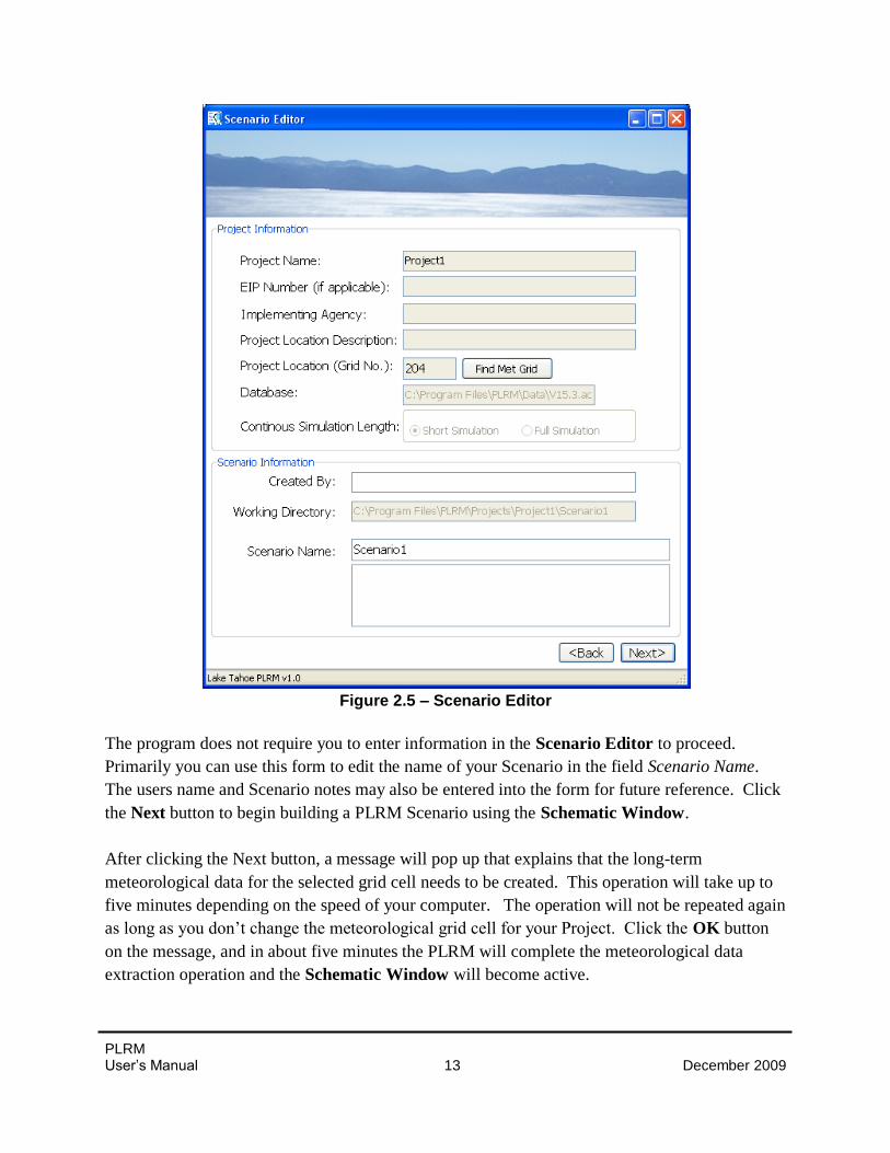
Figure 2.5 – Scenario Editor
The program does not require you to enter information in the Scenario Editor to proceed.
Primarily you can use this form to edit the name of your Scenario in the field Scenario Name.
The users name and Scenario notes may also be entered into the form for future reference. Click
the Next button to begin building a PLRM Scenario using the Schematic Window.
After clicking the Next button, a message will pop up that explains that the long-term
meteorological data for the selected grid cell needs to be created. This operation will take up to
five minutes depending on the speed of your computer. The operation will not be repeated again
as long as you don’t change the meteorological grid cell for your Project. Click the OK button
on the message, and in about five minutes the PLRM will complete the meteorological data
extraction operation and the Schematic Window will become active.
PLRM User’s Manual 14 December 2009
2.2 Developing a Schematic
The Schematic Window is the central input form for the PLRM and allows the modeler to
complete the following functions:
Create a visual representation of their Scenario
Define model elements and drainage routing between model elements
Access input forms for Catchments and SWTs that are created
Run a simulation for a single Scenario
View results for a single Scenario or compare the results for multiple Scenarios
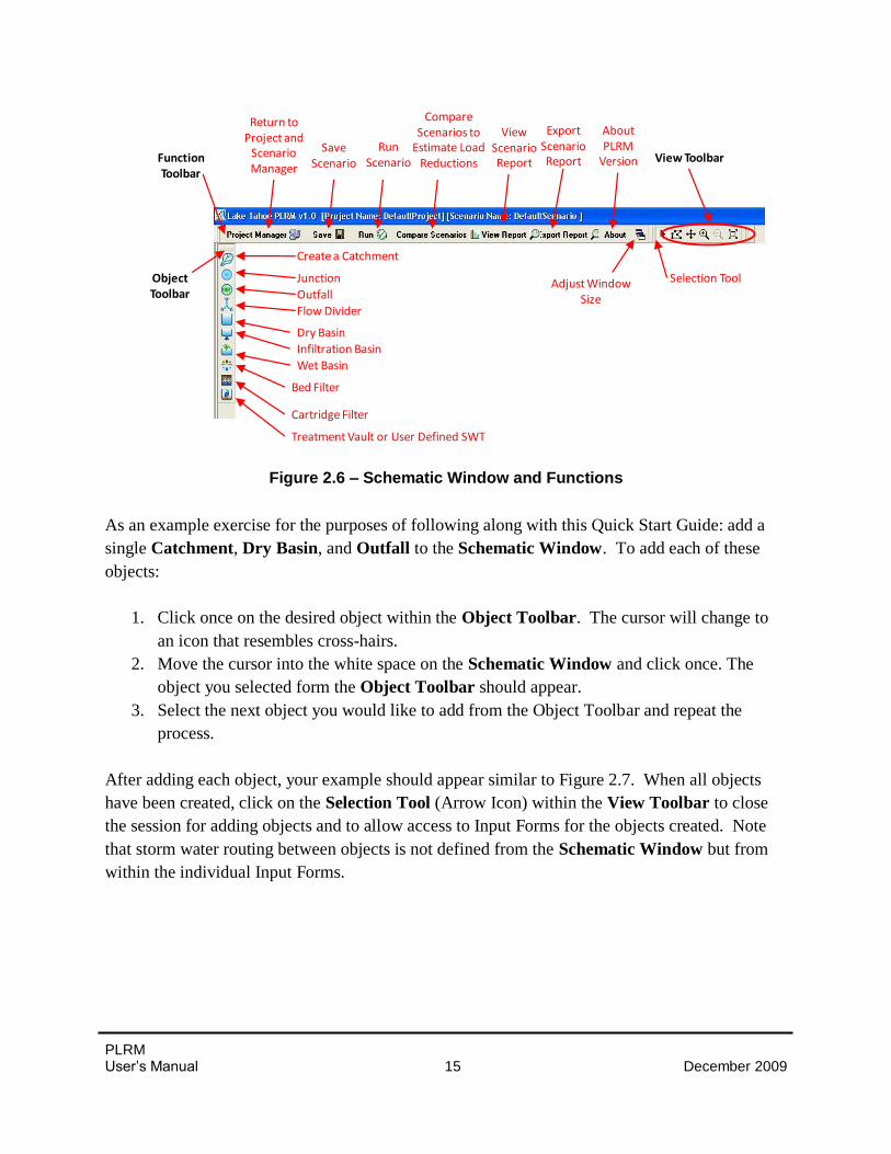
The Schematic Window will appear as shown in Figure 2.6 for a new Scenario. Figure 2.6
provides a brief overview of the functions of the buttons on the Schematic Window. The
buttons within the Schematic Window are organized within three toolbars:
Object Toolbar – Contains all objects that can be added into a PLRM simulation:
Catchments, SWT facilities, Junctions, Flow Dividers, and Outfalls
Function Toolbar – Contains commands for the program to Save, Run, and Display
Results
View Toolbar – Contains buttons to adjust the view. The toolbar also contains the
selection command (arrow icon), which allows selection and movement of specific
objects, as well as access to input forms for specific objects.
The toolbars may be moved and placed anywhere in the Schematic Window.
PLRM User’s Manual 15 December 2009
Figure 2.6 – Schematic Window and Functions
As an example exercise for the purposes of following along with this Quick Start Guide: add a
single Catchment, Dry Basin, and Outfall to the Schematic Window. To add each of these
objects:
1. Click once on the desired object within the Object Toolbar. The cursor will change to
an icon that resembles cross-hairs.
2. Move the cursor into the white space on the Schematic Window and click once. The
object you selected form the Object Toolbar should appear.
3. Select the next object you would like to add from the Object Toolbar and repeat the
process.
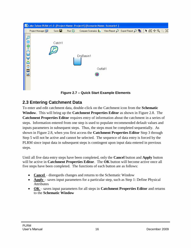
After adding each object, your example should appear similar to Figure 2.7. When all objects
have been created, click on the Selection Tool (Arrow Icon) within the View Toolbar to close
the session for adding objects and to allow access to Input Forms for the objects created. Note
that storm water routing between objects is not defined from the Schematic Window but from
within the individual Input Forms.
Return to Project and
Scenario Manager
Save Scenario
Run Scenario
Compare Scenarios to
Estimate Load Reductions
ViewScenarioReport View Toolbar
Create a Catchment
Outfall
Infiltration Basin
Junction
Flow Divider
Wet Basin
Bed Filter
Cartridge Filter
Treatment Vault or User Defined SWT
Selection Tool
FunctionToolbar
ObjectToolbar
Dry Basin
Adjust WindowSize
ExportScenarioReport
AboutPLRM
Version
PLRM User’s Manual 16 December 2009
Figure 2.7 – Quick Start Example Elements
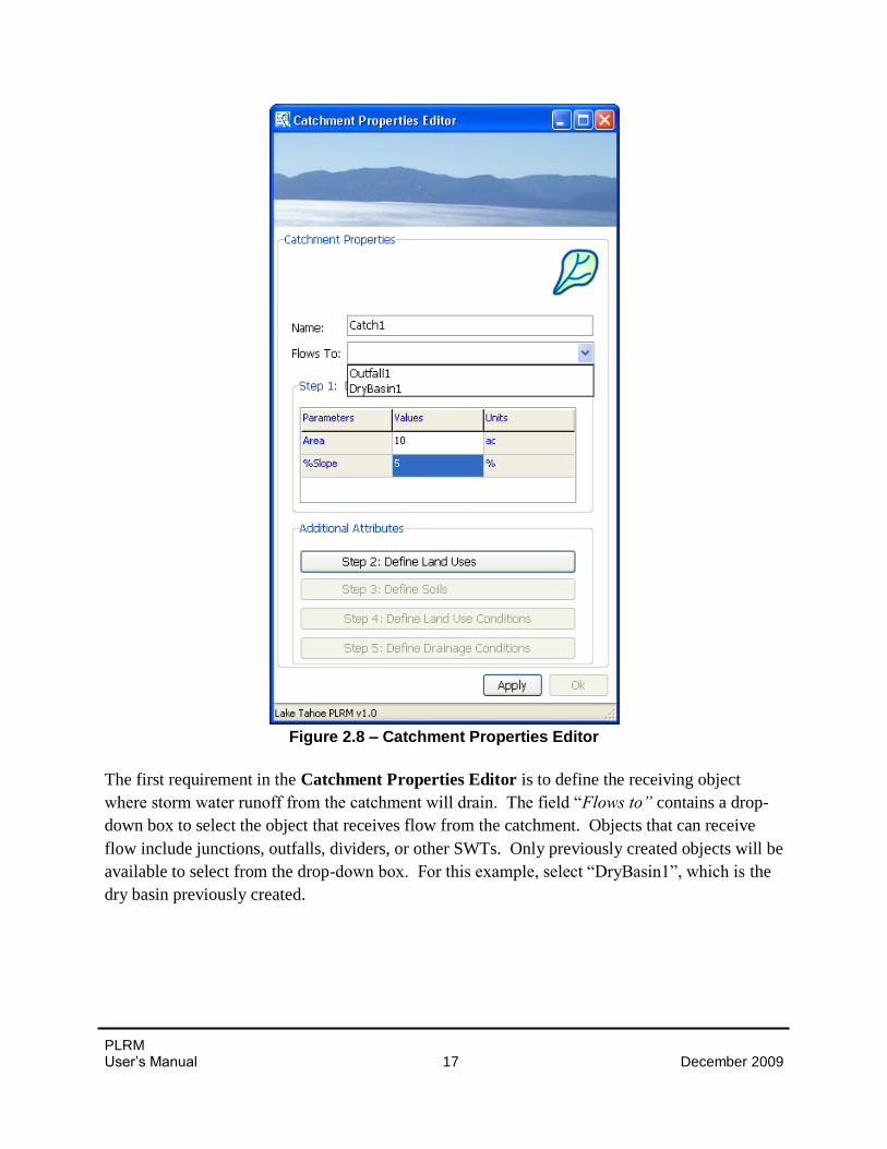
2.3 Entering Catchment Data
To enter and edit catchment data, double-click on the Catchment icon from the Schematic
Window. This will bring up the Catchment Properties Editor as shown in Figure 2.8. The
Catchment Properties Editor requires entry of information about the catchment in a series of
steps. Information entered from one step is used to populate recommended default values and
inputs parameters in subsequent steps. Thus, the steps must be completed sequentially. As
shown in Figure 2.8, when you first access the Catchment Properties Editor Step 3 through
Step 5 will not be active and cannot be selected. The sequence of data entry is forced by the
PLRM since input data in subsequent steps is contingent upon input data entered in previous
steps.
Until all five data entry steps have been completed, only the Cancel button and Apply button
will be active in Catchment Properties Editor. The OK button will become active once all
five steps have been completed. The functions of each button are as follows:
Cancel – disregards changes and returns to the Schematic Window
Apply – saves input parameters for a particular step, such as Step 1: Define Physical
Attributes
OK – saves input parameters for all steps in Catchment Properties Editor and returns to the Schematic Window
PLRM User’s Manual 17 December 2009
Figure 2.8 – Catchment Properties Editor
The first requirement in the Catchment Properties Editor is to define the receiving object
where storm water runoff from the catchment will drain. The field “Flows to” contains a drop-
down box to select the object that receives flow from the catchment. Objects that can receive
flow include junctions, outfalls, dividers, or other SWTs. Only previously created objects will be
available to select from the drop-down box. For this example, select “DryBasin1”, which is the
dry basin previously created.
PLRM User’s Manual 18 December 2009
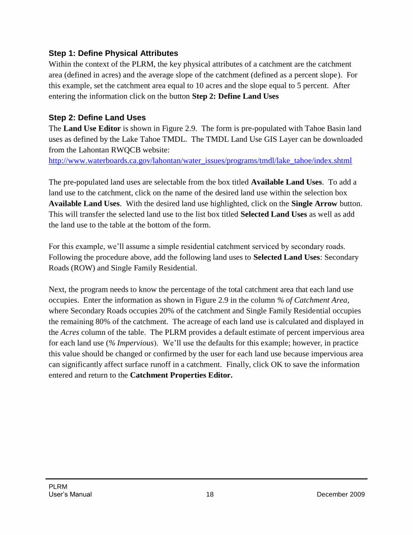
Step 1: Define Physical Attributes
Within the context of the PLRM, the key physical attributes of a catchment are the catchment
area (defined in acres) and the average slope of the catchment (defined as a percent slope). For
this example, set the catchment area equal to 10 acres and the slope equal to 5 percent. After
entering the information click on the button Step 2: Define Land Uses
Step 2: Define Land Uses
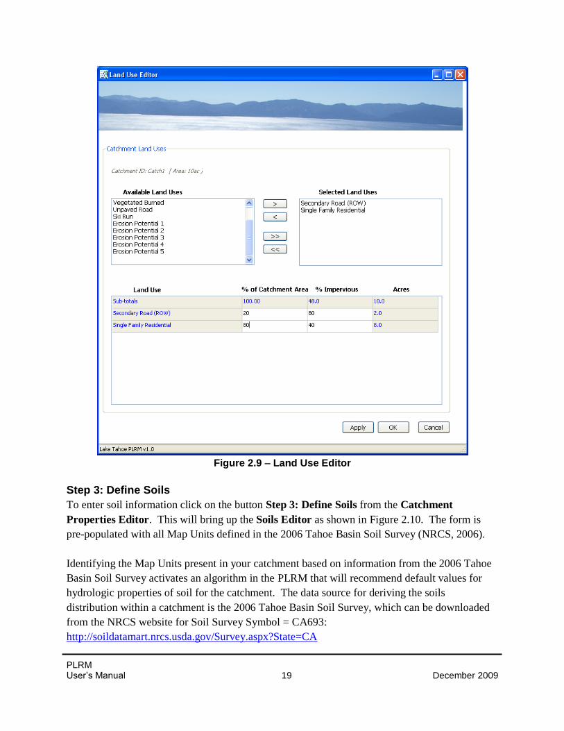
The Land Use Editor is shown in Figure 2.9. The form is pre-populated with Tahoe Basin land
uses as defined by the Lake Tahoe TMDL. The TMDL Land Use GIS Layer can be downloaded
from the Lahontan RWQCB website:
http://www.waterboards.ca.gov/lahontan/water_issues/programs/tmdl/lake_tahoe/index.shtml
The pre-populated land uses are selectable from the box titled Available Land Uses. To add a
land use to the catchment, click on the name of the desired land use within the selection box
Available Land Uses. With the desired land use highlighted, click on the Single Arrow button.
This will transfer the selected land use to the list box titled Selected Land Uses as well as add
the land use to the table at the bottom of the form.
For this example, we’ll assume a simple residential catchment serviced by secondary roads.
Following the procedure above, add the following land uses to Selected Land Uses: Secondary
Roads (ROW) and Single Family Residential.
Next, the program needs to know the percentage of the total catchment area that each land use
occupies. Enter the information as shown in Figure 2.9 in the column % of Catchment Area,
where Secondary Roads occupies 20% of the catchment and Single Family Residential occupies
the remaining 80% of the catchment. The acreage of each land use is calculated and displayed in
the Acres column of the table. The PLRM provides a default estimate of percent impervious area
for each land use (% Impervious). We’ll use the defaults for this example; however, in practice
this value should be changed or confirmed by the user for each land use because impervious area
can significantly affect surface runoff in a catchment. Finally, click OK to save the information
entered and return to the Catchment Properties Editor.
PLRM User’s Manual 19 December 2009
Figure 2.9 – Land Use Editor
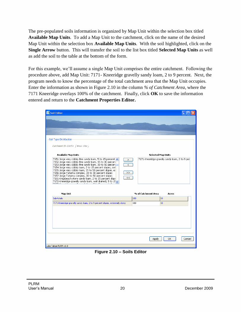
Step 3: Define Soils
To enter soil information click on the button Step 3: Define Soils from the Catchment
Properties Editor. This will bring up the Soils Editor as shown in Figure 2.10. The form is
pre-populated with all Map Units defined in the 2006 Tahoe Basin Soil Survey (NRCS, 2006).
Identifying the Map Units present in your catchment based on information from the 2006 Tahoe
Basin Soil Survey activates an algorithm in the PLRM that will recommend default values for
hydrologic properties of soil for the catchment. The data source for deriving the soils
distribution within a catchment is the 2006 Tahoe Basin Soil Survey, which can be downloaded
from the NRCS website for Soil Survey Symbol = CA693:
http://soildatamart.nrcs.usda.gov/Survey.aspx?State=CA
PLRM User’s Manual 20 December 2009
The pre-populated soils information is organized by Map Unit within the selection box titled
Available Map Units. To add a Map Unit to the catchment, click on the name of the desired
Map Unit within the selection box Available Map Units. With the soil highlighted, click on the
Single Arrow button. This will transfer the soil to the list box titled Selected Map Units as well
as add the soil to the table at the bottom of the form.
For this example, we’ll assume a single Map Unit comprises the entire catchment. Following the
procedure above, add Map Unit: 7171- Kneeridge gravelly sandy loam, 2 to 9 percent. Next, the
program needs to know the percentage of the total catchment area that the Map Unit occupies.
Enter the information as shown in Figure 2.10 in the column % of Catchment Area, where the
7171 Kneeridge overlays 100% of the catchment. Finally, click OK to save the information
entered and return to the Catchment Properties Editor.
Figure 2.10 – Soils Editor
PLRM User’s Manual 21 December 2009
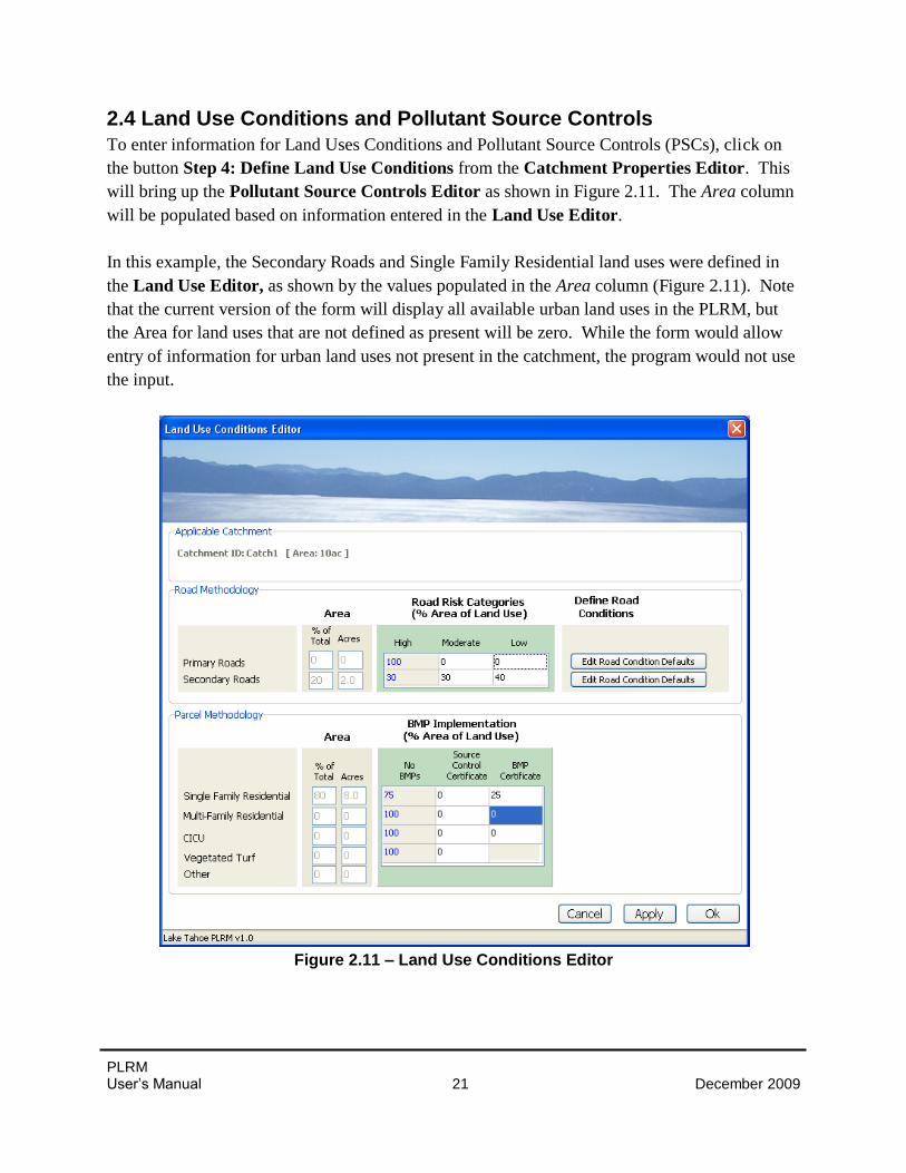
2.4 Land Use Conditions and Pollutant Source Controls
To enter information for Land Uses Conditions and Pollutant Source Controls (PSCs), click on
the button Step 4: Define Land Use Conditions from the Catchment Properties Editor. This
will bring up the Pollutant Source Controls Editor as shown in Figure 2.11. The Area column
will be populated based on information entered in the Land Use Editor.
In this example, the Secondary Roads and Single Family Residential land uses were defined in
the Land Use Editor, as shown by the values populated in the Area column (Figure 2.11). Note
that the current version of the form will display all available urban land uses in the PLRM, but
the Area for land uses that are not defined as present will be zero. While the form would allow
entry of information for urban land uses not present in the catchment, the program would not use
the input.
Figure 2.11 – Land Use Conditions Editor
PLRM User’s Manual 22 December 2009
Two separate methods are accessible from the Land Use Conditions Editor to represent PSCs:
The Road Methodology defines the condition of public right-of-ways, which includes
Primary Road (mostly highways) and Secondary Road land uses. The Road
Methodology allows for separate definitions of the condition of Primary Roads and
Secondary Roads within a catchment.
The Parcel Methodology defines the condition of predominantly private land uses (Single
Family Residential, Multi-Family Residential, CICU, and Vegetated Turf). The Parcel
Methodology allows for separate definitions of private property BMP implementation for
each applicable land use within a catchment.
The discussion below provides a quick example for entering the required information for the two
methodologies. Section 6 of this User’s Manual provides detailed information and guidance on
the definition of input variables and the use of the two methodologies in estimating pollutant
loads from actual catchments.
Road Methodology
The first step in the Road Methodology defines “Road Risk” using three categories (High,
Moderate, and Low). The three categories of Road Risk are related to the anticipated quality of
storm water runoff generated from a road based on key physiographic and anthropogenic
characteristics. Within each risk category, “Road Conditions”
are used to further define expected pollutant concentrations.
For this example, enter the Road Risk distribution for
Secondary Roads as shown in Figure 2.11: High = 30%;
Moderate = 30%; and Low = 40%. Note that the value in the
High column is calculated based on the values entered in the
Moderate and Low columns (see Key Concept Box). After
completing the Road Risk input, we’ll move on to defining the
condition of the Secondary Roads within the catchment.
Select the button Edit Road Conditions Defaults to bring up
the Road Conditions Editor as shown in Figure 2.12. Make
sure you select the button for Secondary Roads and not the
button for Primary Roads.
Key Concept Box
The PLRM code was written to
ensure percentages in tables add
up to 100%. Fields with text in
blue with a shaded background
are not editable and are
calculated based on information
entered in other associated fields.
For example, in the Road Risk
table the value for “High” is
calculated as: (100% minus
value in Moderate column minus
value in Low column).
PLRM User’s Manual 23 December 2009
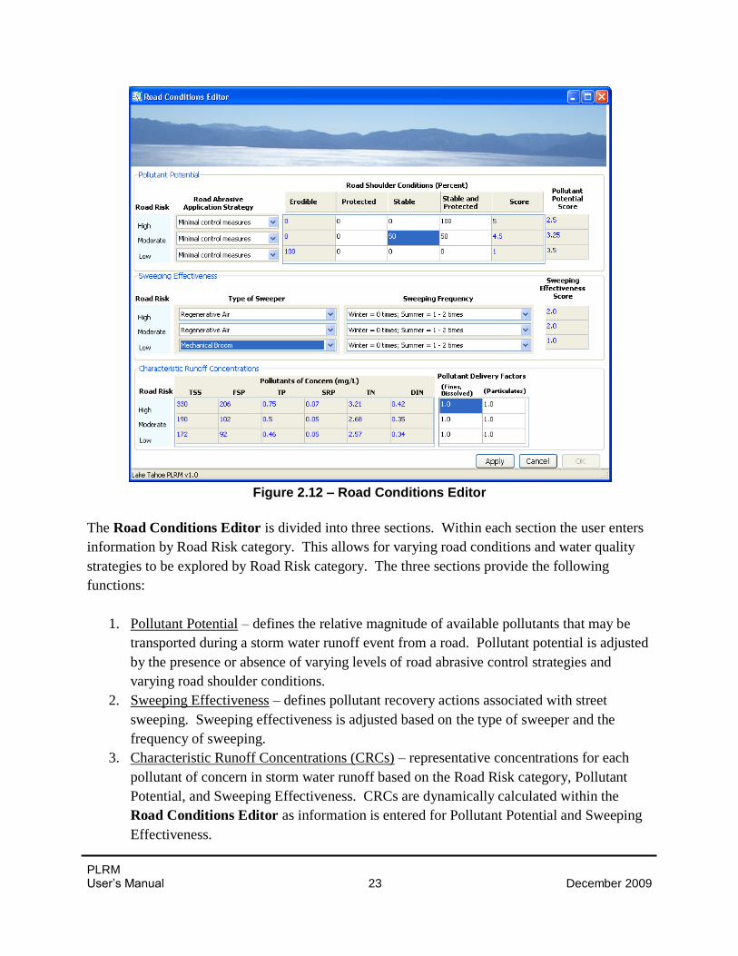
Figure 2.12 – Road Conditions Editor
The Road Conditions Editor is divided into three sections. Within each section the user enters
information by Road Risk category. This allows for varying road conditions and water quality
strategies to be explored by Road Risk category. The three sections provide the following
functions:
1. Pollutant Potential – defines the relative magnitude of available pollutants that may be
transported during a storm water runoff event from a road. Pollutant potential is adjusted
by the presence or absence of varying levels of road abrasive control strategies and
varying road shoulder conditions.
2. Sweeping Effectiveness – defines pollutant recovery actions associated with street
sweeping. Sweeping effectiveness is adjusted based on the type of sweeper and the
frequency of sweeping.
3. Characteristic Runoff Concentrations (CRCs) – representative concentrations for each
pollutant of concern in storm water runoff based on the Road Risk category, Pollutant
Potential, and Sweeping Effectiveness. CRCs are dynamically calculated within the
Road Conditions Editor as information is entered for Pollutant Potential and Sweeping
Effectiveness.
PLRM User’s Manual 24 December 2009
For this example, enter the information as shown in Figure 2.12. Note how the CRCs
dynamically change for each Road Risk category as information about the Pollutant Potential
and Street Sweeping activities are entered. After completing data entry in the Road Conditions
Editor to match Figure 2.12, select the OK button to save the information, close the form, and
return to the Pollutant Source Controls Editor (Figure 2.11).
Parcel Methodology
The Parcel Methodology defines the amount of private property BMP implementation for each
urban land use present in the catchment. BMP implementation is entered in the Pollutant
Source Controls Editor in the table titled BMP Implementation as the percent of area of the
land use. There are two types of BMP Implementation as defined by TRPA, which issues BMP
certificates:
Source Control Certificate – a property has completed PSC implementation (i.e. pervious
areas of the property are stabilized). However, the property has recognized constraints
that do not allow for HSC implementation to the typical standard (i.e. storage of runoff
from 20-year 1-hour storm on the property)
BMP Retrofit Certificate – a property has completed both PSC and HSC implementation
to the typical standard
For this example, we’ll assume that the Single Family Residential land use has 25% of its total
area under BMP Certificate compliance. Enter the information to reproduce Figure 2.11 then
Click the OK button to save the information entered and return to the Catchment Properties
Editor.
2.5 Hydrology and Hydrologic Source Controls
To enter information on Hydrologic Properties and HSCs, click on the button Step 5: Define
Drainage Conditions from the Catchment Properties Editor. This will bring up the Drainage
Conditions Editor as shown in Figure 2.13. There are two tabs on the Drainage Conditions
Editor: 1) Road Methodology; and 2) Parcel Methodology. Click on the Road Methodology tab,
and this will bring up the screen shown in Figure 2.13. Similar to the Land Use Conditions
Editor, the Drainage Conditions Editor includes an Area column and an Impervious Area
column with values populated based on information entered in the Land Use Editor. Note that
the form will display all available urban land uses for the specific methodology, but the Area for
land uses that are not defined as present will be zero. While the form would allow entry of
information for urban land uses not present in the catchment, the program would not use the
input.
PLRM User’s Manual 25 December 2009
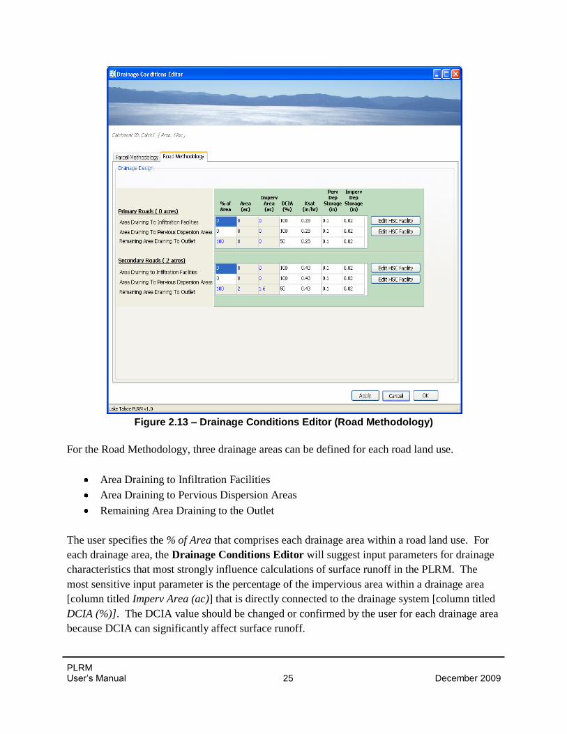
Figure 2.13 – Drainage Conditions Editor (Road Methodology)
For the Road Methodology, three drainage areas can be defined for each road land use.
Area Draining to Infiltration Facilities
Area Draining to Pervious Dispersion Areas
Remaining Area Draining to the Outlet
The user specifies the % of Area that comprises each drainage area within a road land use. For
each drainage area, the Drainage Conditions Editor will suggest input parameters for drainage
characteristics that most strongly influence calculations of surface runoff in the PLRM. The
most sensitive input parameter is the percentage of the impervious area within a drainage area
[column titled Imperv Area (ac)] that is directly connected to the drainage system [column titled
DCIA (%)]. The DCIA value should be changed or confirmed by the user for each drainage area
because DCIA can significantly affect surface runoff.
PLRM User’s Manual 26 December 2009
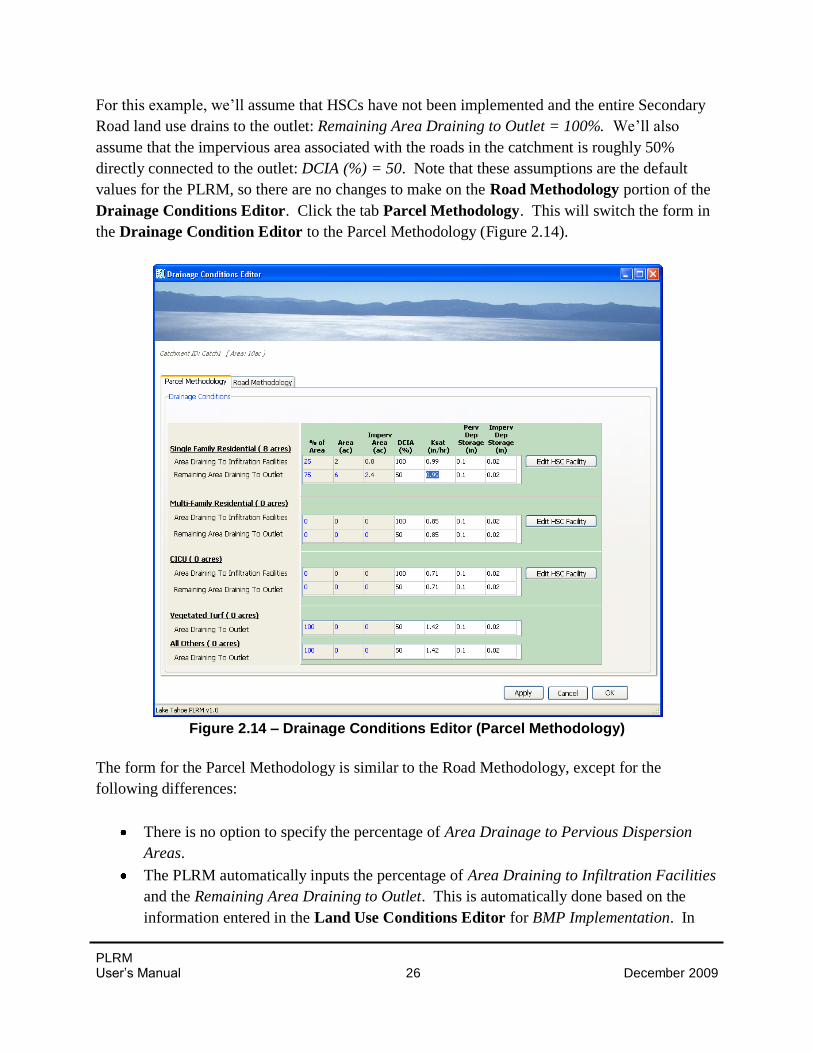
For this example, we’ll assume that HSCs have not been implemented and the entire Secondary
Road land use drains to the outlet: Remaining Area Draining to Outlet = 100%. We’ll also
assume that the impervious area associated with the roads in the catchment is roughly 50%
directly connected to the outlet: DCIA (%) = 50. Note that these assumptions are the default
values for the PLRM, so there are no changes to make on the Road Methodology portion of the
Drainage Conditions Editor. Click the tab Parcel Methodology. This will switch the form in
the Drainage Condition Editor to the Parcel Methodology (Figure 2.14).
Figure 2.14 – Drainage Conditions Editor (Parcel Methodology)
The form for the Parcel Methodology is similar to the Road Methodology, except for the
following differences:
There is no option to specify the percentage of Area Drainage to Pervious Dispersion
Areas.
The PLRM automatically inputs the percentage of Area Draining to Infiltration Facilities
and the Remaining Area Draining to Outlet. This is automatically done based on the
information entered in the Land Use Conditions Editor for BMP Implementation. In
PLRM User’s Manual 27 December 2009
our example, we entered in the Land Use Conditions Editor that 25% of the Single
Family Residential area had BMP Retrofit Certificates. Based on the definition of the
BMP Retrofit Certificates, this means that 25% of the area for that land use is draining to
infiltration facilities.
For this example, we’ll assume that the impervious area associated with Remaining Area
Draining to Outlet in Single Family Residential is roughly 50% directly connected to the outlet:
DCIA (%) = 50. Note that these assumptions are the default values for the PLRM, so there are
no changes to make on the Parcel Methodology portion of the Drainage Conditions Editor.
Click the OK button to close the form and return to the Catchment Properties Editor.
At this point, all information required for the catchment has been completed. On the Catchment
Properties Editor, click the OK button to close the form and return to the Schematic Window.
2.6 Storm Water Treatment
There are a number of Storm Water Treatment (SWT) facilities than can be simulated in the
PLRM. For this Quick Start Guide, we’ll go over how to input information for a Dry Basin.
Section 8 describes inputs parameters for all SWT facilities in the PLRM.
To enter and edit SWT data for a Dry Basin, double-click on the Dry Basin icon we
created from the Schematic Window. This will bring up the Dry Basin Editor as
shown in Figure 2.15.
The first requirement in the Dry Basin Editor is to define the receiving object where surface
water leaving the SWT will drain (treated and bypassed flows). The field “Flows to” contains a
drop-down box to select the object that receives flow from the Dry Basin. Objects that can
receive flow include junctions, outfalls, dividers, or other SWTs. Only previously created
objects will be available to select from the drop-down box.
For this example, select the Outfall you previously created in
the Schematic Window. If you didn’t rename your Outfall,
it will be named “Outfall1” in the drop-down box.
Note that Outfalls are required objects in any PLRM
simulation because the PLRM calculates and summarizes
average annual runoff volumes and pollutant loading of a
Scenario at the Outfalls defined for that Scenario. If storm
water runoff is not routed to Outfalls then the Scenario
Report (Section 9.1 of this Manual) will not include all
runoff and pollutant loading.
Key Concept Box
Outfalls are required objects
because the PLRM calculates
and summarizes average annual
runoff volumes and pollutant
loading at Outfalls. If storm
water runoff is not routed to an
Outfall, then the Scenario Report
will not include all runoff and
pollutant loading for the
Scenario.
PLRM User’s Manual 28 December 2009
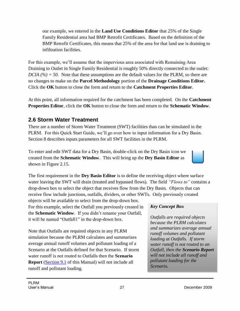
Figure 2.15 – Dry Basin Editor
The Dry Basin Editor requires entry of key Design Parameters to simulate the performance of
the Dry Basin for capturing and treating runoff. Key Design Parameters include:
Water Quality Volume – storage capacity below the bypass outlet designed for water quality treatment
Footprint – surface area that will typically be inundated; approximately the area at the
average design depth
Infiltration Rate – characteristic rate of infiltration expected over the life-span of the SWT while factoring in assumptions for anticipated or committed maintenance
PLRM User’s Manual 29 December 2009
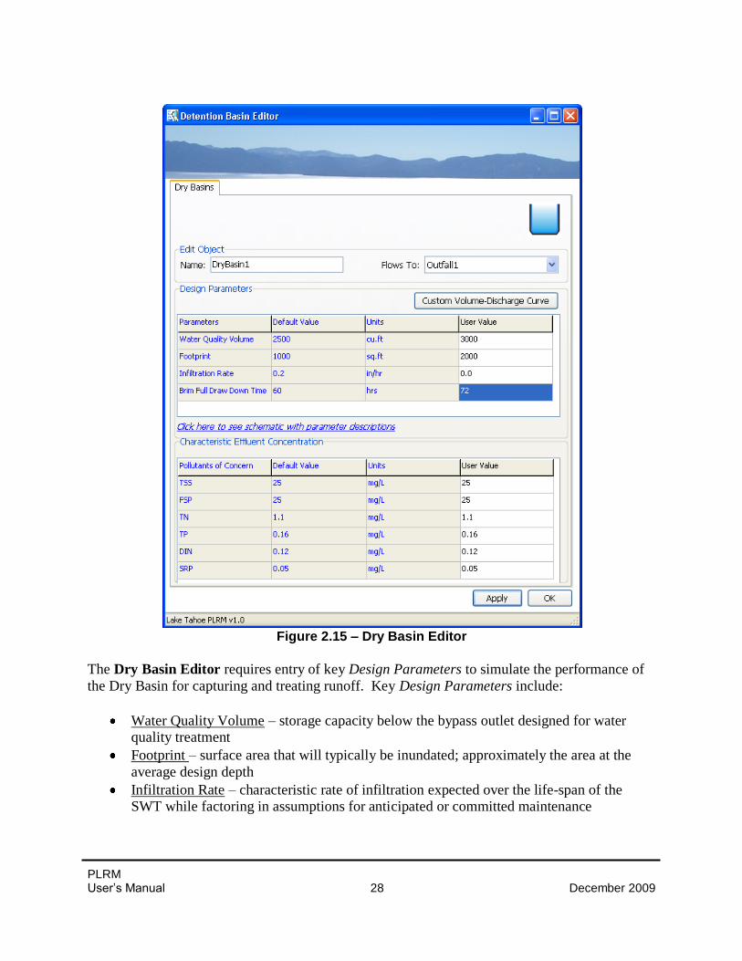
Brim Full Draw Down Time – time it takes for the Water Quality Volume to completely drain through treatment outlets(s) as treated storm water runoff without consideration of
the infiltration rate
An illustration of how the Design Parameters relate to the representation of a Dry Basin in the
PLRM is accessible from the Dry Basin Editor by clicking on “Click here to see schematic with
parameters descriptions”. Clicking on the link will bring up Figure 2.16.
Figure 2.16 – Dry Basin Representation in PLRM
For this example, enter the information as shown in Figure 2.15.
Water Quality Volume = 3,000 cubic feet
Footprint = 2,000 cubic feet
Infiltration Rate = 0.0 inches/hour
Brim Full Draw Down Time = 72 hours
After completing data entry in the Dry Basin Editor to match Figure 2.15, click the OK button
to close the form and return to the Schematic Window.
PLRM User’s Manual 30 December 2009
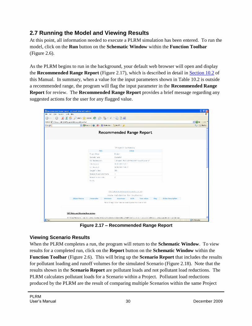
2.7 Running the Model and Viewing Results
At this point, all information needed to execute a PLRM simulation has been entered. To run the
model, click on the Run button on the Schematic Window within the Function Toolbar
(Figure 2.6).
As the PLRM begins to run in the background, your default web browser will open and display
the Recommended Range Report (Figure 2.17), which is described in detail in Section 10.2 of
this Manual. In summary, when a value for the input parameters shown in Table 10.2 is outside
a recommended range, the program will flag the input parameter in the Recommended Range
Report for review. The Recommended Range Report provides a brief message regarding any
suggested actions for the user for any flagged value.
Figure 2.17 – Recommended Range Report
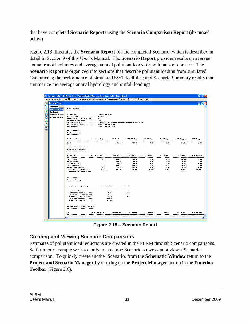
Viewing Scenario Results
When the PLRM completes a run, the program will return to the Schematic Window. To view
results for a completed run, click on the Report button on the Schematic Window within the
Function Toolbar (Figure 2.6). This will bring up the Scenario Report that includes the results
for pollutant loading and runoff volumes for the simulated Scenario (Figure 2.18). Note that the
results shown in the Scenario Report are pollutant loads and not pollutant load reductions. The
PLRM calculates pollutant loads for a Scenario within a Project. Pollutant load reductions
produced by the PLRM are the result of comparing multiple Scenarios within the same Project
PLRM User’s Manual 31 December 2009
that have completed Scenario Reports using the Scenario Comparison Report (discussed
below).
Figure 2.18 illustrates the Scenario Report for the completed Scenario, which is described in
detail in Section 9 of this User’s Manual. The Scenario Report provides results on average
annual runoff volumes and average annual pollutant loads for pollutants of concern. The
Scenario Report is organized into sections that describe pollutant loading from simulated
Catchments; the performance of simulated SWT facilities; and Scenario Summary results that
summarize the average annual hydrology and outfall loadings.
Figure 2.18 – Scenario Report
Creating and Viewing Scenario Comparisons
Estimates of pollutant load reductions are created in the PLRM through Scenario comparisons.
So far in our example we have only created one Scenario so we cannot view a Scenario
comparison. To quickly create another Scenario, from the Schematic Window return to the
Project and Scenario Manager by clicking on the Project Manager button in the Function
Toolbar (Figure 2.6).
PLRM User’s Manual 32 December 2009
In the Project and Scenario Manager, expand the tree
structure for our Project by clicking once on the plus sign
next to the name of our Project. Then click on the name
of the Scenario we created to highlight the Scenario.
Finally, with the Scenario highlighted click on the button
Copy Selected. This will copy our Scenario into the
Project and open the Scenario Editor. In the Scenario
Editor for the field Scenario Name, rename the Scenario
to “Scenario2” and click the Next button. The Schematic
Window will now be shown with the copied Scenario.
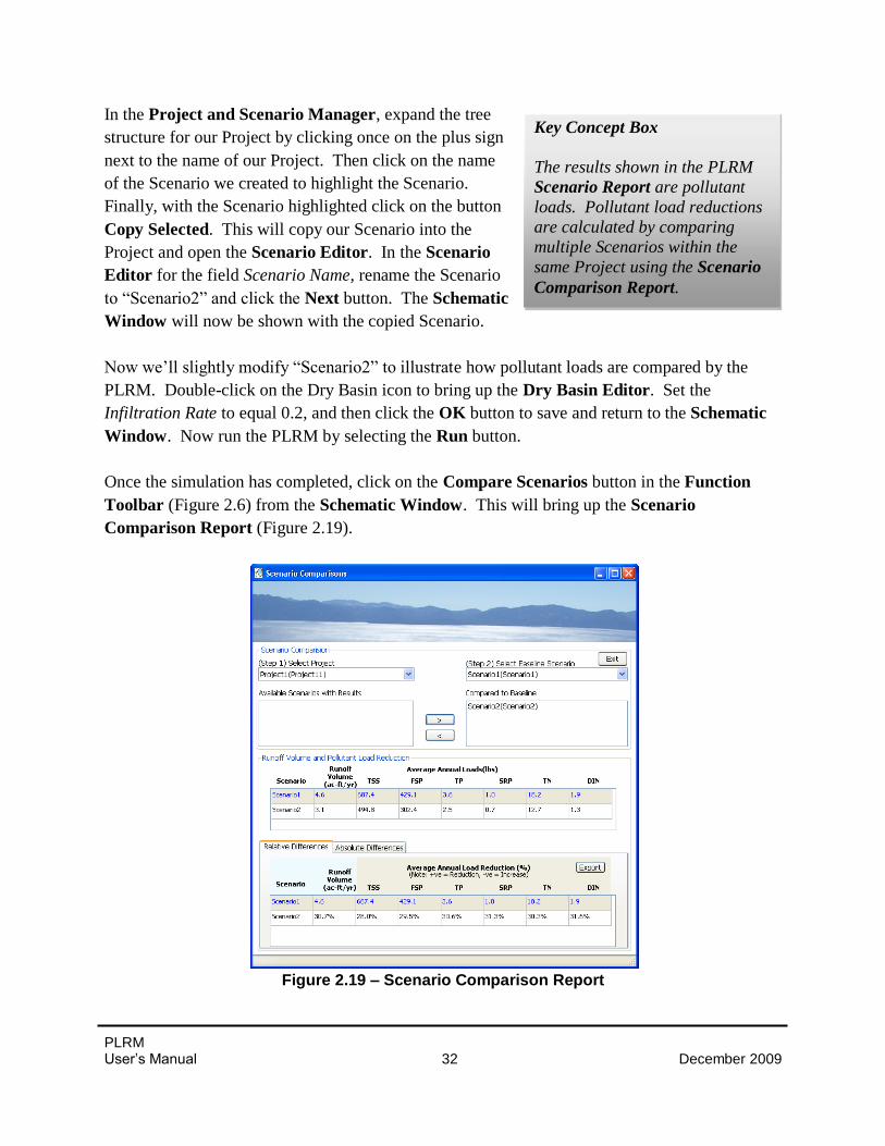
Now we’ll slightly modify “Scenario2” to illustrate how pollutant loads are compared by the
PLRM. Double-click on the Dry Basin icon to bring up the Dry Basin Editor. Set the
Infiltration Rate to equal 0.2, and then click the OK button to save and return to the Schematic
Window. Now run the PLRM by selecting the Run button.
Once the simulation has completed, click on the Compare Scenarios button in the Function
Toolbar (Figure 2.6) from the Schematic Window. This will bring up the Scenario
Comparison Report (Figure 2.19).
Figure 2.19 – Scenario Comparison Report
Key Concept Box
The results shown in the PLRM
Scenario Report are pollutant
loads. Pollutant load reductions
are calculated by comparing
multiple Scenarios within the
same Project using the Scenario
Comparison Report.
PLRM User’s Manual 33 December 2009
To compare Scenarios for our Project complete the following steps in order.
1. In the drop-down box titled (Step 1) Select Project, select our Project. After selecting the
Project, you’ll notice that our Scenarios will appear in the selection box titled Available
Scenarios and Results.
2. In the drop-down box titled (Step 2) Select Baseline Scenario, select “Scenario1”. This
will be the baseline Scenario (typically the existing condition) to which other Scenarios
will be compared for calculating pollutant load reductions.
3. In the selection box titled Available Scenarios and Results, click on “Scenario2” to
highlight it. Then click on the Single Arrow button pointing to the list box titled
Compared to Baseline. This will move “Scenario2” into the list box and populate the
tables below.
Completing the steps above will populate the pollutant load reductions tables in the Scenario
Comparison Report as shown in Figure 2.19. Two tables are provided in the Scenario
Comparison Report that report 1) average annual loads and 2) the relative difference of
pollutant loads among Scenarios. To export the output in this form to an editable format, click
on the button Export and specify the location for saving the file.
PLRM User’s Manual 34 December 2009
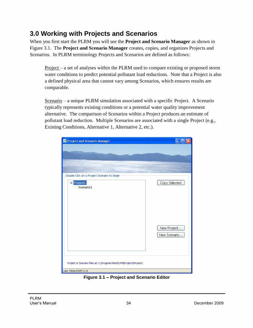
3.0 Working with Projects and Scenarios When you first start the PLRM you will see the Project and Scenario Manager as shown in
Figure 3.1. The Project and Scenario Manager creates, copies, and organizes Projects and
Scenarios. In PLRM terminology Projects and Scenarios are defined as follows:
Project – a set of analyses within the PLRM used to compare existing or proposed storm
water conditions to predict potential pollutant load reductions. Note that a Project is also
a defined physical area that cannot vary among Scenarios, which ensures results are
comparable.
Scenario – a unique PLRM simulation associated with a specific Project. A Scenario
typically represents existing conditions or a potential water quality improvement
alternative. The comparison of Scenarios within a Project produces an estimate of
pollutant load reduction. Multiple Scenarios are associated with a single Project (e.g.,
Existing Conditions, Alternative 1, Alternative 2, etc.).
Figure 3.1 – Project and Scenario Editor
PLRM User’s Manual 35 December 2009
The following functions are executed by the Project and Scenario Manager:
New Project – Creates a new Project and launches the Project Editor. The PLRM will
provide a default name for the Project, which can be renamed within the Project Editor.
New Scenario – Creates a new Scenario and launches the Scenario Editor. The PLRM
will provide a default name for the Scenario, which can be renamed within the Scenario
Editor. Note that this function only works when a Project is selected in the Project and
Scenario Manager because a Scenario must be associated with a Project.
Copy Selected – Copies and adds the selected Project or Scenario to the Project and
Scenario Manager. The PLRM will provide a default name for a copied Project or
Scenario, which can be renamed.
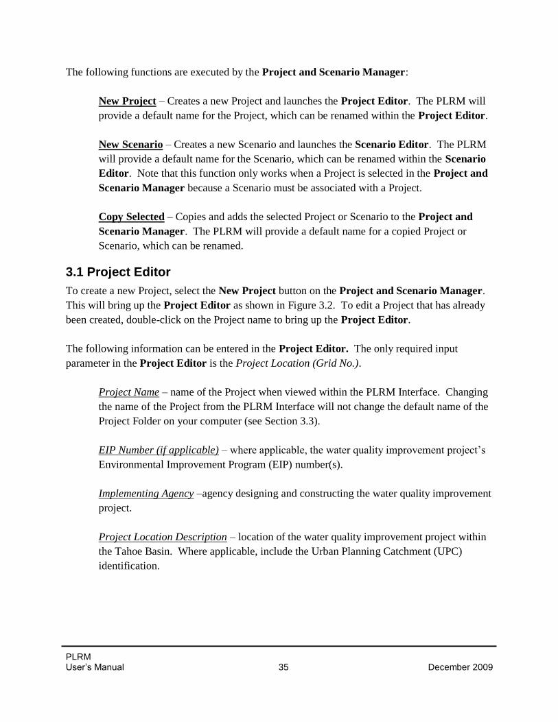
3.1 Project Editor
To create a new Project, select the New Project button on the Project and Scenario Manager.
This will bring up the Project Editor as shown in Figure 3.2. To edit a Project that has already
been created, double-click on the Project name to bring up the Project Editor.
The following information can be entered in the Project Editor. The only required input
parameter in the Project Editor is the Project Location (Grid No.).
Project Name – name of the Project when viewed within the PLRM Interface. Changing
the name of the Project from the PLRM Interface will not change the default name of the
Project Folder on your computer (see Section 3.3).
EIP Number (if applicable) – where applicable, the water quality improvement project’s
Environmental Improvement Program (EIP) number(s).
Implementing Agency –agency designing and constructing the water quality improvement
project.
Project Location Description – location of the water quality improvement project within
the Tahoe Basin. Where applicable, include the Urban Planning Catchment (UPC)
identification.
PLRM User’s Manual 36 December 2009
Figure 3.2 – Project Editor
The following functions are executed by the Project Editor:
Project Location (Grid No.) – defines the physical location of the water quality
improvement project in the Tahoe Basin by designating a PLRM meteorological grid cell.
Clicking on the button Find Met Grid from the Project Editor will activate an image of
the Tahoe Basin overlain with the PLRM meteorological grid. Each grid cell is 800
meters by 800 meters. You can zoom into the image to find your project area and the
associated grid cell. Select and enter the grid cell that is closest to the centroid of your
project area. Only one grid cell can be defined for a Project.
Defining the grid cell of your Project will execute a temperature and precipitation
algorithm in the PLRM that will provide pre-processed hourly precipitation and
temperature data for your specified location for Water Years 1989 through 2006.
Precipitation data is extrapolated to your grid cell using the historical time series of
precipitation from the most applicable SnoTel gage and a relationship derived from the
Parameter-elevation Regressions on Independent Slopes Model (PRISM), developed at
PLRM User’s Manual 37 December 2009
Oregon State University (PRISM, 2008). Temperature data is extrapolated to your grid
cell using the historical time series of temperature from the most applicable SnoTel gage
and a temperature lapse rate developed for use in the Lake Tahoe Watershed Model.
Additional documentation describing the precipitation and temperature algorithms can be
found in the PLRM Model Development Documentation (Section 3 and Appendix A).
Database – defines the PLRM Database used for the Project. The Default Parameters
included within the PLRM Database are not recommended for modification by the user
unless the modifications are done to incorporate new or additional data. Maintaining
consistent Default Parameters in the PLRM Database is recommended because it will
help to maintain consistency of results generated by multiple user’s across multiple
project areas. Additionally, the structure of the PLRM Database should not be modified,
only data within the database. Section 11 of this Manual describes the PLRM Database.
Continuous Simulation Length – this function provides an option to reduce the run time
of a PLRM simulation by reducing the length of the continuous simulation. A Short
Simulation will run a subset of the current PLRM time series - Water Years 1990 through
1996. A Full Simulation will run the complete PLRM time series - Water Years 1989
through 2006. The intent of providing the Short Simulation option is to allow the user to
decrease run times when creating and testing a Scenario. The time period for the Short
Simulation was selected because it includes Water Years with above average, below
average, and average precipitation. In most cases the Short Simulation will produce
output with similar results to a Full Simulation. Once the Scenarios have been developed
and quality assured, the user should switch to the Full Simulation option to assess and
report output.
Save Project Info – Saves information entered in the Project Editor and returns to the
Project and Scenario Manager.
3.2 Scenario Editor
The Project and Scenario Manager organizes Projects and the Scenarios associated with each
Project using a tree structure. The PLRM will automatically create the first Scenario for a
Project with the default name “Scenario1”. If Scenarios are not visible in the Project and
Scenario Manager, click once on the plus sign next to the name of the applicable Project to
expand the tree structure. To create a new Scenario for the Project, with the Project highlighted,
click on the New Scenario button in the Project and Scenario Manager.
You can access the Scenario Editor (Figure 3.3) by either creating a new Scenario or double-
clicking on an existing Scenario. The PLRM does not require you to enter information in the
PLRM User’s Manual 38 December 2009
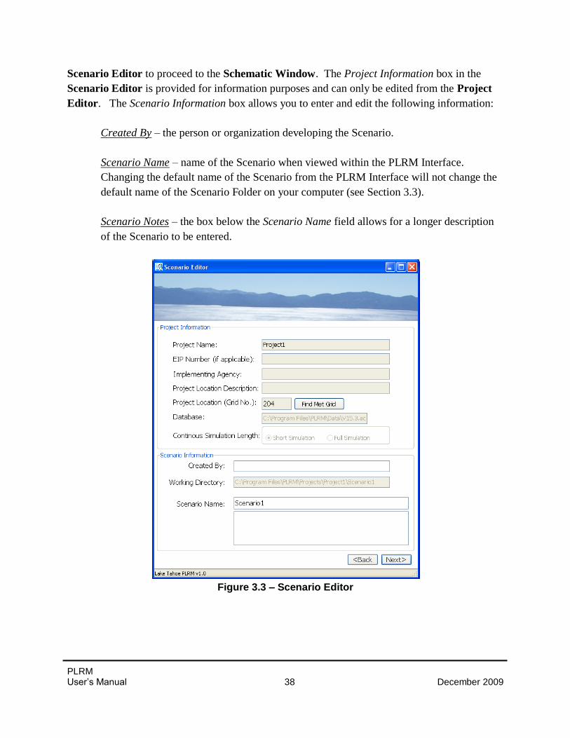
Scenario Editor to proceed to the Schematic Window. The Project Information box in the
Scenario Editor is provided for information purposes and can only be edited from the Project
Editor. The Scenario Information box allows you to enter and edit the following information:
Created By – the person or organization developing the Scenario.
Scenario Name – name of the Scenario when viewed within the PLRM Interface.
Changing the default name of the Scenario from the PLRM Interface will not change the
default name of the Scenario Folder on your computer (see Section 3.3).
Scenario Notes – the box below the Scenario Name field allows for a longer description
of the Scenario to be entered.
Figure 3.3 – Scenario Editor
PLRM User’s Manual 39 December 2009
The following functions are executed by the Scenario Editor:
Back – Returns to the Project and Scenario Manager.
Next – Proceeds to the Schematic Window where
you can start building a PLRM Scenario. If you
select a new meteorological grid cell in the Project
Editor, when you click the NEXT button on the
Scenario Editor a message will pop up explaining
that the long-term meteorological data for the
selected grid cell needs to be created. Creating the
hourly time series of precipitation and temperature
data will take up to five minutes depending on the
speed of your computer. Click the OK button on
the message, and in about five minutes the PLRM
will complete the meteorological algorithm and the
Schematic Window will become active. The PLRM
will save the time series of precipitation and temperature for the meteorological grid cell
to your computer. With the time series saved, the operation will not be repeated the next
time you click the NEXT button from the Scenario Editor. The operation will be
repeated if you change the meteorological grid cell in the Project Editor.
3.3 Managing Projects and Scenarios on Your Computer
This section describes how to manage Projects and Scenarios outside of the Project and
Scenario Manager. To conserve programming resources for PLRM Version 1, some file
management functions (e.g., delete a Project or Scenario) are not yet incorporated into the
Project and Scenario Manager but can be completed manually using Windows Explorer.
When the PLRM is installed on your computer, a directory named “PLRM”
is created in a user-specified location. Within the PLRM directory, three
directories are created: Data, Engine, and Projects. The Projects Directory is
used to store files related to a specific Project and Scenario. When a user
creates a new Project, a Project Folder is created in the Projects Directory. When a user creates a
new Scenario, a Scenario Folder is created and placed in the associated Project Folder. Project
and Scenario Folders are named sequentially by the PLRM (e.g., Project1, Project2, Scenario1,
Scenario2, etc.) and should never be moved or renamed from Windows Explorer.
Within the PLRM Interface, a Project or Scenario can be renamed using the Project and
Scenario Editors. This will create an alias for the Project or Scenario when viewed within the
PLRM Interface. However, it will not rename a Project or Scenario Folder on your computer.
Key Concept Box
The PLRM executes an algorithm
to create hourly time series data
of precipitation and temperature
for your project location. This
operation will take up to five
minutes depending on the speed
of your computer. The data is
saved and the operation will not
be repeated when the same
meteorological grid cell is used.
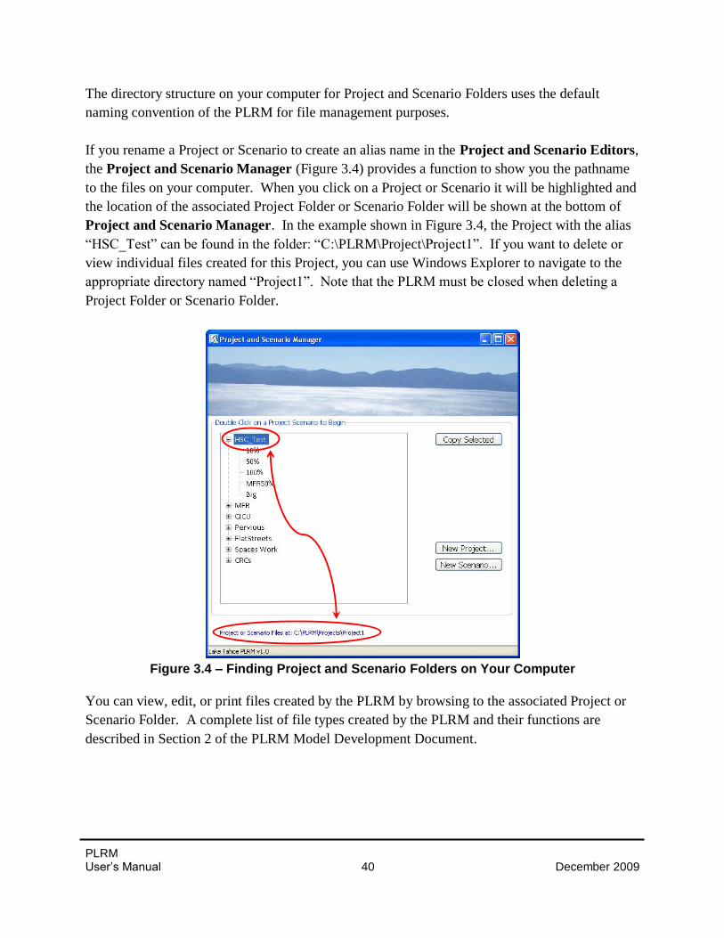
PLRM User’s Manual 40 December 2009
The directory structure on your computer for Project and Scenario Folders uses the default
naming convention of the PLRM for file management purposes.
If you rename a Project or Scenario to create an alias name in the Project and Scenario Editors,
the Project and Scenario Manager (Figure 3.4) provides a function to show you the pathname
to the files on your computer. When you click on a Project or Scenario it will be highlighted and
the location of the associated Project Folder or Scenario Folder will be shown at the bottom of
Project and Scenario Manager. In the example shown in Figure 3.4, the Project with the alias
“HSC_Test” can be found in the folder: “C:\PLRM\Project\Project1”. If you want to delete or
view individual files created for this Project, you can use Windows Explorer to navigate to the
appropriate directory named “Project1”. Note that the PLRM must be closed when deleting a
Project Folder or Scenario Folder.
Figure 3.4 – Finding Project and Scenario Folders on Your Computer
You can view, edit, or print files created by the PLRM by browsing to the associated Project or
Scenario Folder. A complete list of file types created by the PLRM and their functions are
described in Section 2 of the PLRM Model Development Document.
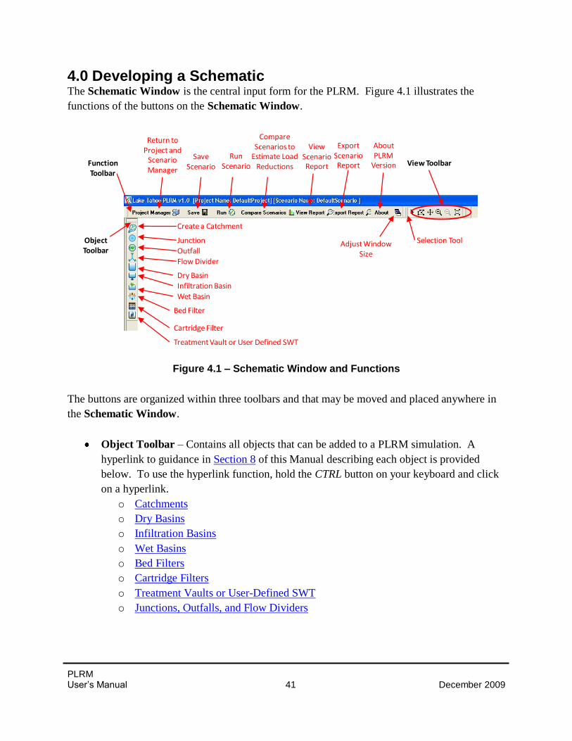
PLRM User’s Manual 41 December 2009
4.0 Developing a Schematic The Schematic Window is the central input form for the PLRM. Figure 4.1 illustrates the
functions of the buttons on the Schematic Window.
Figure 4.1 – Schematic Window and Functions
The buttons are organized within three toolbars and that may be moved and placed anywhere in
the Schematic Window.
Object Toolbar – Contains all objects that can be added to a PLRM simulation. A
hyperlink to guidance in Section 8 of this Manual describing each object is provided
below. To use the hyperlink function, hold the CTRL button on your keyboard and click
on a hyperlink.
o Catchments
o Dry Basins
o Infiltration Basins
o Wet Basins
o Bed Filters
o Cartridge Filters
o Treatment Vaults or User-Defined SWT
o Junctions, Outfalls, and Flow Dividers
Return to Project and
Scenario Manager
Save Scenario
Run Scenario
Compare Scenarios to
Estimate Load Reductions
ViewScenarioReport View Toolbar
Create a Catchment
Outfall
Infiltration Basin
Junction
Flow Divider
Wet Basin
Bed Filter
Cartridge Filter
Treatment Vault or User Defined SWT
Selection Tool
FunctionToolbar
ObjectToolbar
Dry Basin
Adjust WindowSize
ExportScenarioReport
AboutPLRM
Version
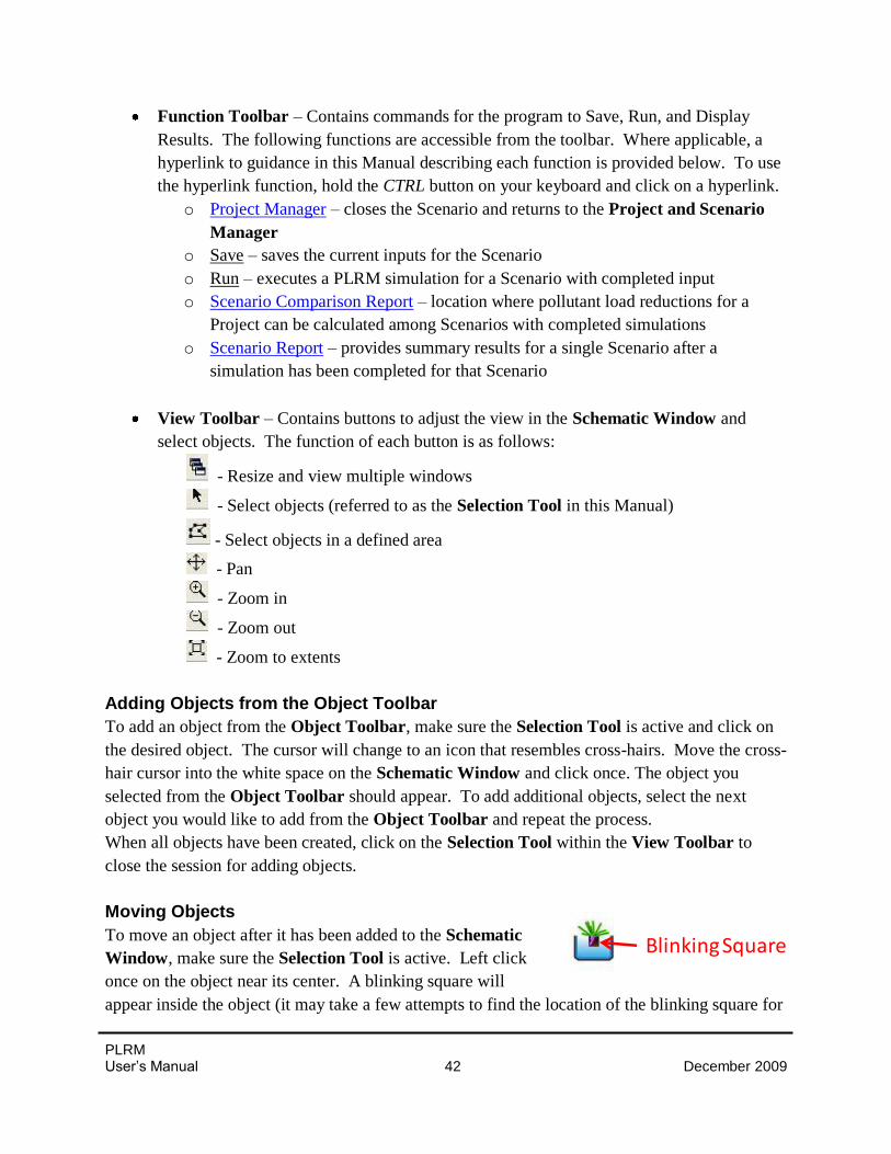
PLRM User’s Manual 42 December 2009
Function Toolbar – Contains commands for the program to Save, Run, and Display
Results. The following functions are accessible from the toolbar. Where applicable, a
hyperlink to guidance in this Manual describing each function is provided below. To use
the hyperlink function, hold the CTRL button on your keyboard and click on a hyperlink.
o Project Manager – closes the Scenario and returns to the Project and Scenario
Manager
o Save – saves the current inputs for the Scenario
o Run – executes a PLRM simulation for a Scenario with completed input
o Scenario Comparison Report – location where pollutant load reductions for a
Project can be calculated among Scenarios with completed simulations
o Scenario Report – provides summary results for a single Scenario after a
simulation has been completed for that Scenario
View Toolbar – Contains buttons to adjust the view in the Schematic Window and
select objects. The function of each button is as follows:
- Resize and view multiple windows
- Select objects (referred to as the Selection Tool in this Manual)
- Select objects in a defined area
- Pan
- Zoom in
- Zoom out
- Zoom to extents
Adding Objects from the Object Toolbar
To add an object from the Object Toolbar, make sure the Selection Tool is active and click on
the desired object. The cursor will change to an icon that resembles cross-hairs. Move the cross-
hair cursor into the white space on the Schematic Window and click once. The object you
selected from the Object Toolbar should appear. To add additional objects, select the next
object you would like to add from the Object Toolbar and repeat the process.
When all objects have been created, click on the Selection Tool within the View Toolbar to
close the session for adding objects.
Moving Objects
To move an object after it has been added to the Schematic
Window, make sure the Selection Tool is active. Left click
once on the object near its center. A blinking square will
appear inside the object (it may take a few attempts to find the location of the blinking square for
Blinking Square
PLRM User’s Manual 43 December 2009
different objects). Left click again on the blinking square and hold the left click button. You
should now be able to move the object by moving your mouse.
Deleting Objects
To delete an object after it has been added to the Schematic Window, make sure the Selection
Tool is active. Left click once on the object near its center. A blinking square will appear inside
the object (it may take a few attempts to find the location of the blinking square for different
objects). Hit the Delete button on your keyboard. The PLRM will ask you to confirm the
deletion of the object. Select YES to delete the object and NO to cancel.
Accessing Input Forms for Objects
To access Input Forms for each object after it has been added to the Schematic Window,
double-click on the object. In most cases, you can double-click anywhere on the object to bring
up the relevant Input Form.
Defining Storm Water Routing Between Objects
Storm water routing between objects is not defined from the Schematic Window but rather from
within the individual Input Forms. For each object there is drop-down box titled “Flows to” that
will include all other objects that have been added to the
Schematic Window that can receive flow. Objects that
can receive flow include junctions, outfalls, dividers, or
other SWTs. Examples of objects that cannot receive
flow include 1) any Catchment, or 2) any object cannot be
routed to itself. The user should first add all objects
envisioned for a Scenario to the Schematic Window then
define storm water routing of individual objects from the
Input Forms. This approach will ensure that all potential
objects that could receive flow are accessible from each
Input Form when defining storm water routing.
Key Concept Box
The routing between objects is
not defined from the Schematic
Window but rather from within
the individual Input Forms for
each object using a drop-down
box titled “Flows to:”. The user
should first add objects
envisioned for a Scenario to the
Schematic Window then define
storm water routing using Input
Forms.
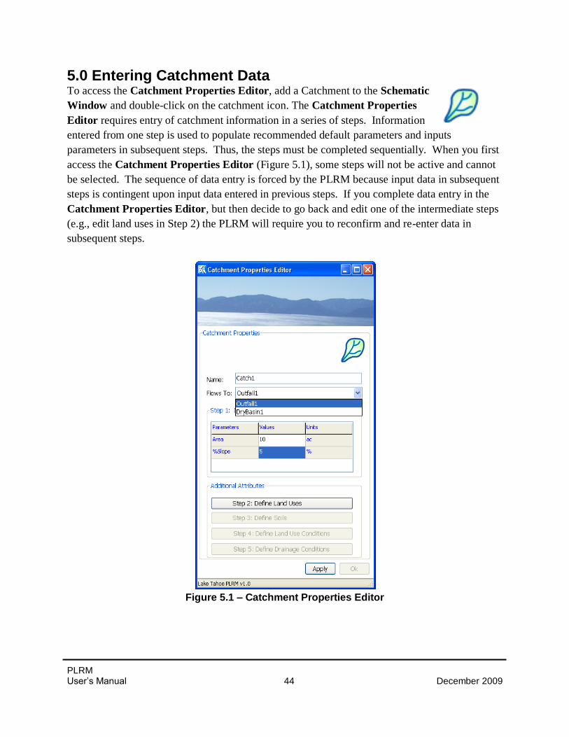
PLRM User’s Manual 44 December 2009
5.0 Entering Catchment Data To access the Catchment Properties Editor, add a Catchment to the Schematic
Window and double-click on the catchment icon. The Catchment Properties
Editor requires entry of catchment information in a series of steps. Information
entered from one step is used to populate recommended default parameters and inputs
parameters in subsequent steps. Thus, the steps must be completed sequentially. When you first
access the Catchment Properties Editor (Figure 5.1), some steps will not be active and cannot
be selected. The sequence of data entry is forced by the PLRM because input data in subsequent
steps is contingent upon input data entered in previous steps. If you complete data entry in the
Catchment Properties Editor, but then decide to go back and edit one of the intermediate steps
(e.g., edit land uses in Step 2) the PLRM will require you to reconfirm and re-enter data in
subsequent steps.
Figure 5.1 – Catchment Properties Editor
PLRM User’s Manual 45 December 2009
There are five steps for data entry in the Catchment Properties Editor. Steps 1 through 3 are
described in this section of the Manual. Input parameters described in this section are typically
developed during the Formulating and Evaluating Alternatives (FEA) process and are available
within a project’s Existing Conditions Analysis Memorandum (ECAM). Therefore, the methods
to develop input parameters for Steps 1 through 3 are not described in detail here. The
formulation of alternatives should also include the input parameters described in this section if
alternatives change catchment boundaries relative to existing conditions, or if alternatives change
land uses.
A hyperlink to each step is provided below.
Step 1: Define Physical Attributes
Step 2: Define Land Uses
Step 3: Define Soils
Step 4: Define Land Use Conditions - is
described in Section 6 of this Manual.
Step 5: Define Drainage Conditions - described
in Section 7 of this Manual.
Until all five data entry steps have been completed, only
the Cancel button and Apply button will be active in
Catchment Properties Editor. The OK button will
become active once all five steps have been completed.
The functions of each button are as follows:
Cancel – disregards changes and returns to the Schematic Window
Apply – saves input parameters for a particular step, such as Step 1: Define Physical Attributes
OK – saves input parameters for all steps in Catchment Properties Editor and returns to the Schematic Window
5.1 Physical Attributes
Physical attributes include the storm water routing of the catchment, the size of the catchment,
and the average slope of the catchment.
The following are input parameters for Step 1:
Name – you can edit the default name of the catchment if desired. By default, the PLRM
will name catchments sequentially as Catch1, Catch2, etc.
Key Concept Box
The sequence of data entry within
the Catchment Properties Editor
is forced by the PLRM because
input data in subsequent steps is
contingent upon input data
entered in previous steps. If you
complete data entry in the
Catchment Properties Editor,
but then decide to go back and
edit one of the intermediate steps
(e.g., edit land uses in Step 2) the
PLRM will require you to
reconfirm and re-enter data in
subsequent steps.
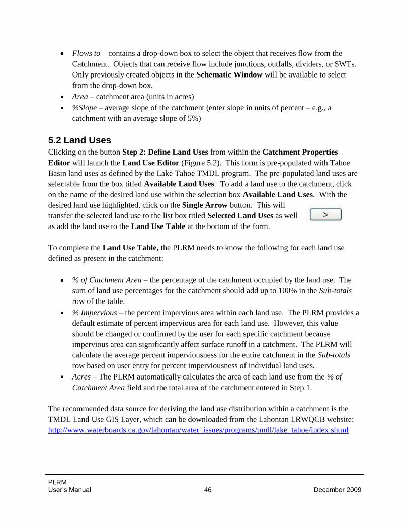
PLRM User’s Manual 46 December 2009
Flows to – contains a drop-down box to select the object that receives flow from the
Catchment. Objects that can receive flow include junctions, outfalls, dividers, or SWTs.
Only previously created objects in the Schematic Window will be available to select
from the drop-down box.
Area – catchment area (units in acres)
%Slope – average slope of the catchment (enter slope in units of percent – e.g., a
catchment with an average slope of 5%)
5.2 Land Uses
Clicking on the button Step 2: Define Land Uses from within the Catchment Properties
Editor will launch the Land Use Editor (Figure 5.2). This form is pre-populated with Tahoe
Basin land uses as defined by the Lake Tahoe TMDL program. The pre-populated land uses are
selectable from the box titled Available Land Uses. To add a land use to the catchment, click
on the name of the desired land use within the selection box Available Land Uses. With the
desired land use highlighted, click on the Single Arrow button. This will
transfer the selected land use to the list box titled Selected Land Uses as well
as add the land use to the Land Use Table at the bottom of the form.
To complete the Land Use Table, the PLRM needs to know the following for each land use
defined as present in the catchment:
% of Catchment Area – the percentage of the catchment occupied by the land use. The
sum of land use percentages for the catchment should add up to 100% in the Sub-totals
row of the table.
% Impervious – the percent impervious area within each land use. The PLRM provides a
default estimate of percent impervious area for each land use. However, this value
should be changed or confirmed by the user for each specific catchment because
impervious area can significantly affect surface runoff in a catchment. The PLRM will
calculate the average percent imperviousness for the entire catchment in the Sub-totals
row based on user entry for percent imperviousness of individual land uses.
Acres – The PLRM automatically calculates the area of each land use from the % of
Catchment Area field and the total area of the catchment entered in Step 1.
The recommended data source for deriving the land use distribution within a catchment is the
TMDL Land Use GIS Layer, which can be downloaded from the Lahontan LRWQCB website:
http://www.waterboards.ca.gov/lahontan/water_issues/programs/tmdl/lake_tahoe/index.shtml
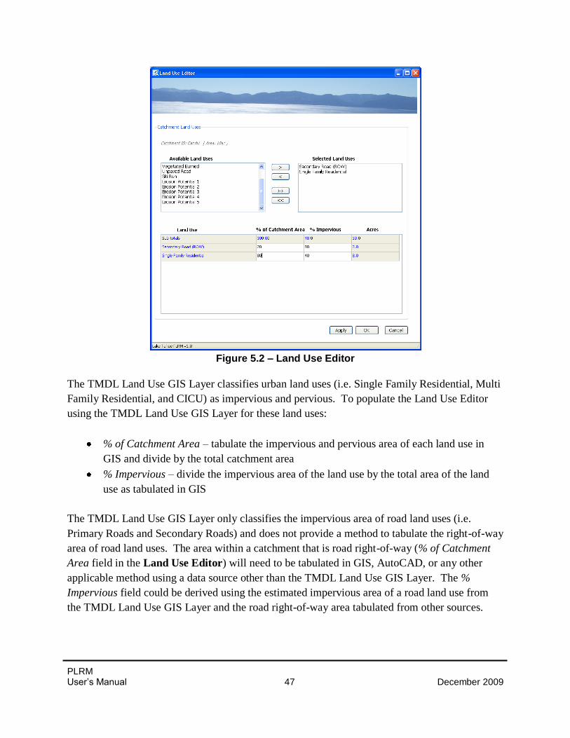
PLRM User’s Manual 47 December 2009
Figure 5.2 – Land Use Editor
The TMDL Land Use GIS Layer classifies urban land uses (i.e. Single Family Residential, Multi
Family Residential, and CICU) as impervious and pervious. To populate the Land Use Editor
using the TMDL Land Use GIS Layer for these land uses:
% of Catchment Area – tabulate the impervious and pervious area of each land use in
GIS and divide by the total catchment area
% Impervious – divide the impervious area of the land use by the total area of the land
use as tabulated in GIS
The TMDL Land Use GIS Layer only classifies the impervious area of road land uses (i.e.
Primary Roads and Secondary Roads) and does not provide a method to tabulate the right-of-way
area of road land uses. The area within a catchment that is road right-of-way (% of Catchment
Area field in the Land Use Editor) will need to be tabulated in GIS, AutoCAD, or any other
applicable method using a data source other than the TMDL Land Use GIS Layer. The %
Impervious field could be derived using the estimated impervious area of a road land use from
the TMDL Land Use GIS Layer and the road right-of-way area tabulated from other sources.
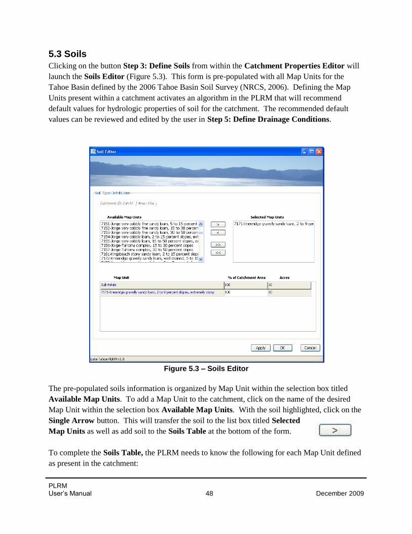
PLRM User’s Manual 48 December 2009
5.3 Soils
Clicking on the button Step 3: Define Soils from within the Catchment Properties Editor will
launch the Soils Editor (Figure 5.3). This form is pre-populated with all Map Units for the
Tahoe Basin defined by the 2006 Tahoe Basin Soil Survey (NRCS, 2006). Defining the Map
Units present within a catchment activates an algorithm in the PLRM that will recommend
default values for hydrologic properties of soil for the catchment. The recommended default
values can be reviewed and edited by the user in Step 5: Define Drainage Conditions.
Figure 5.3 – Soils Editor
The pre-populated soils information is organized by Map Unit within the selection box titled
Available Map Units. To add a Map Unit to the catchment, click on the name of the desired
Map Unit within the selection box Available Map Units. With the soil highlighted, click on the
Single Arrow button. This will transfer the soil to the list box titled Selected
Map Units as well as add soil to the Soils Table at the bottom of the form.
To complete the Soils Table, the PLRM needs to know the following for each Map Unit defined
as present in the catchment:

PLRM User’s Manual 49 December 2009
% of Catchment Area – the percentage of the catchment occupied by the soil. The sum of
percentages for all soils in the catchment should add up to 100% in the Sub-totals row of
the table.
Acres – The PLRM automatically calculates the area of each soil using % of Catchment
Area field and the total area of the catchment entered in Step 1.
The data source for deriving the soils distribution within a catchment is the 2006 Tahoe Basin
Soil Survey, which can be downloaded from the NRCS website for Soil Survey Symbol =
CA693: http://soildatamart.nrcs.usda.gov/Survey.aspx?State=CA
An alternative method for developing the soils distribution information is to use the Web Soil
Survey tools created by the NRCS. The tools are accessible at:
http://websoilsurvey.nrcs.usda.gov/app/HomePage.htm
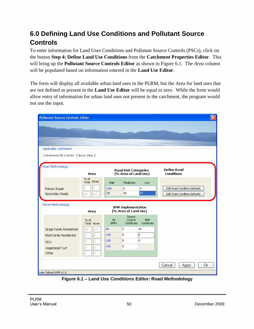
PLRM User’s Manual 50 December 2009
6.0 Defining Land Use Conditions and Pollutant Source
Controls To enter information for Land Uses Conditions and Pollutant Source Controls (PSCs), click on
the button Step 4: Define Land Use Conditions from the Catchment Properties Editor. This
will bring up the Pollutant Source Controls Editor as shown in Figure 6.1. The Area column
will be populated based on information entered in the Land Use Editor.
The form will display all available urban land uses in the PLRM, but the Area for land uses that
are not defined as present in the Land Use Editor will be equal to zero. While the form would
allow entry of information for urban land uses not present in the catchment, the program would
not use the input.
Figure 6.1 – Land Use Conditions Editor: Road Methodology
PLRM User’s Manual 51 December 2009
Two separate methods are accessible from the Land Use Conditions Editor to represent PSCs:
The Road Methodology defines the condition of public right-of-ways, which includes
Primary Roads and Secondary Roads. Primary Roads include all state and federal
highways, as well as major arterial roads in the Tahoe Basin (e.g., Pioneer Trail).
Secondary Roads are all urban roads in the Tahoe Basin that are not Primary Roads. The
Road Methodology allows for separate definition of the condition of Primary Roads and
Secondary Roads within a catchment. Note that the methodology applies to primary and
secondary roads as a land use, and thus includes paved and unpaved areas within the
right-of-way and not just the road pavement areas.
The Parcel Methodology defines the condition of predominantly private land uses
(Single Family Residential, Multi-Family Residential, CICU, and Vegetated Turf). The
Parcel Methodology allows for separate definition of private property BMP
implementation for each applicable land use within a catchment.
6.1 Road Methodology The PLRM Road Methodology contains new concepts
and methods to predict the quality of runoff generated
from roads. The methodology is based on the hypothesis
that the condition of roads can be correlated to
characteristic runoff concentrations (CRCs) for
pollutants of concern. The key variables that are use to
predict CRCs include physiographic characteristics,
PSCs applied to the road shoulder, road abrasive
application practices, and pollutant recovery activities.
A detailed discussion of the research and development of
the Road Methodology is provided in the PLRM Model
Development Document – Section 5.1, Appendix B, and
Appendix C. This section of the User’s Manual describes how to apply the Road Methodology
in the PLRM as it pertains to Pollutant Generation and PSC Implementation. The definitions and
methods in this section are focused on defining CRCs rather than loads, and are not influenced
by the connectivity of impervious area to downstream receiving waters. Connectivity is an
important factor in estimating pollutant loads, and Section 7 of this Manual (Define Drainage
Conditions) describes the appropriate place and methods in the PLRM to incorporate impervious
area connectivity.
Key Concept Box
The definitions and methods in
Section 6.1 are focused on
defining CRCs rather than
pollutant loads. The methods are
not influenced by the
connectivity of impervious area
to downstream receiving waters.
Section 7 describes the
appropriate place and methods in
the PLRM to incorporate
impervious area connectivity.
PLRM User’s Manual 52 December 2009
6.1.1 Road Risk Categories As shown in the Land Use Conditions Editor (Figure 6.1), the first step in the Road
Methodology is to define the distribution of Road Risk for Primary Roads and Secondary Roads.
Road Risk is used to categorize the pollutant potential of a road segment based on physiographic
characteristics that are assumed to most strongly influence the quality of storm water generated,
specifically: Slope, Traffic Density, and Adjacent Land Use. The rationale for selecting these
physiographic characteristics to define Road Risk is summarized as follows:
Slope – Steeper sloped roads generally receive more frequent road abrasive applications.
Additionally, storm water on steeper sloped roads is conveyed at higher velocities, which
increases the potential for scour and pollutant transport.
Traffic Density – Highly trafficked roads receive more frequent road abrasive
applications and are subject to increased road shoulder disturbance through human and
vehicle traffic. Sediment on highly trafficked roads will be subject to more pulverization
and therefore a higher fraction of FSP is anticipated in storm water runoff.
Adjacent Land Use – Roads adjacent to denser urban land uses (e.g. Commercial and
Multi-Family Residential) tend to have more frequent road abrasive applications and are
subject to increased road shoulder disturbance through human and vehicle traffic.
Figure 6.2 displays the default Road Risk GIS Layer developed from these parameters for use in
the PLRM. You can use the default Road Risk Layer in GIS to develop an estimated distribution
of Road Risk Categories in your catchment for Primary and Secondary Roads. The default Road
Risk GIS Layer is available for download along with the PLRM setup program and
documentation from: http://www.tiims.org/TIIMS-Sub-Sites/PLRM.aspx
Road Risk can be defined separately for Primary Roads and Secondary Roads in the Land Use
Conditions Editor (Figure 6.1). The distribution of Road Risk is entered as percentages of the
total road land use (i.e. Primary Roads or Secondary Roads) using categories of High Risk,
Moderate Risk, and Low Risk. The sum of percentages for the three Road Risk Categories
should equate to 100%.
In practical terms, a High Risk Road relative to a Moderate Risk Road is 1) steeper, 2) has higher
average traffic volumes; and/or 3) has denser urban land uses adjacent to the road. Conversely,
a Low Risk Road relative to a Moderate Risk Road is 1) flatter, 2) has lower average traffic
volumes, and/or 3) has less dense urban land uses adjacent to the road.
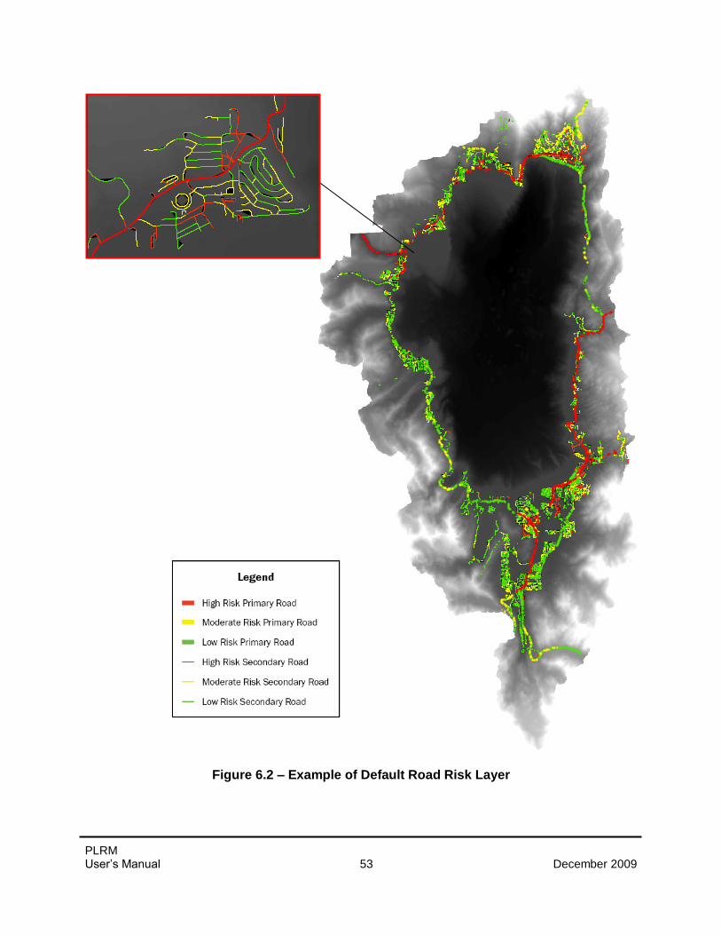
PLRM User’s Manual 53 December 2009
Figure 6.2 – Example of Default Road Risk Layer
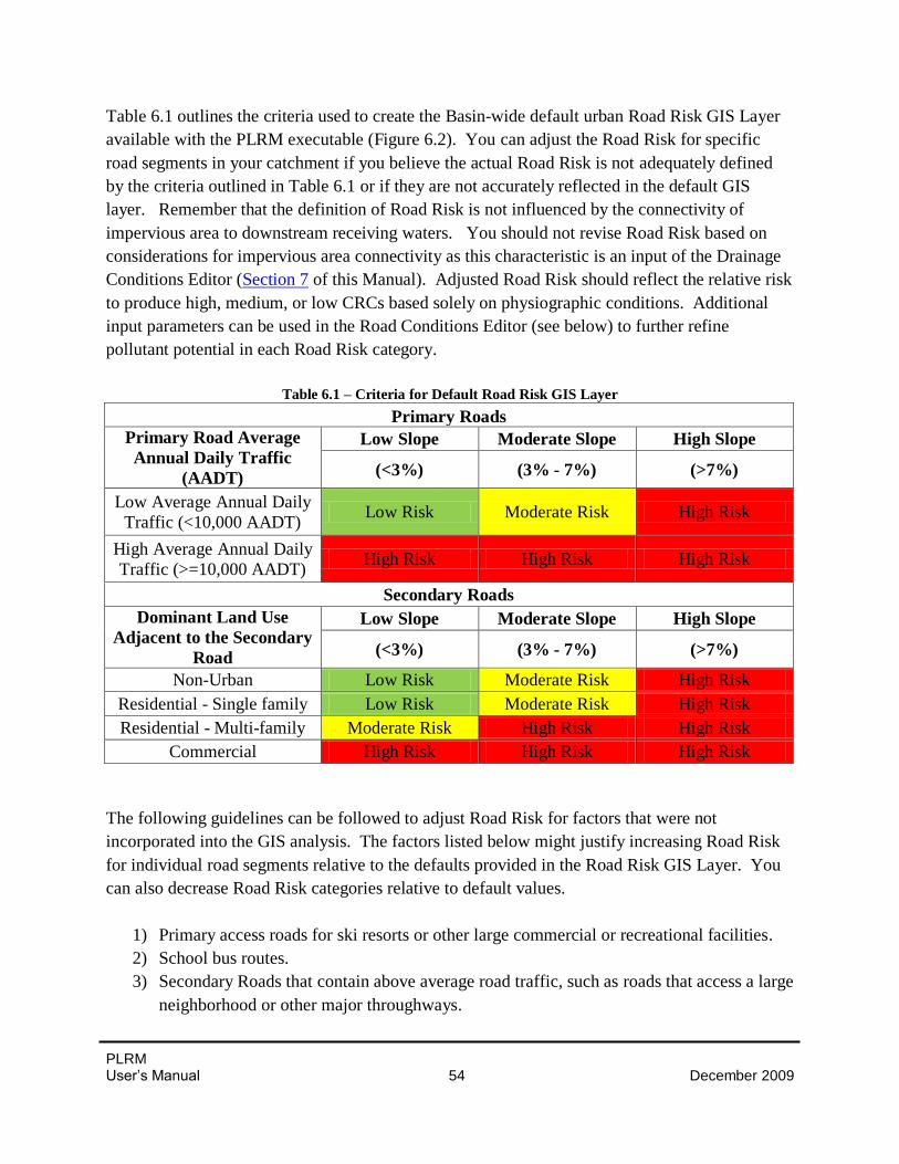
PLRM User’s Manual 54 December 2009
Table 6.1 outlines the criteria used to create the Basin-wide default urban Road Risk GIS Layer
available with the PLRM executable (Figure 6.2). You can adjust the Road Risk for specific
road segments in your catchment if you believe the actual Road Risk is not adequately defined
by the criteria outlined in Table 6.1 or if they are not accurately reflected in the default GIS
layer. Remember that the definition of Road Risk is not influenced by the connectivity of
impervious area to downstream receiving waters. You should not revise Road Risk based on
considerations for impervious area connectivity as this characteristic is an input of the Drainage
Conditions Editor (Section 7 of this Manual). Adjusted Road Risk should reflect the relative risk
to produce high, medium, or low CRCs based solely on physiographic conditions. Additional
input parameters can be used in the Road Conditions Editor (see below) to further refine
pollutant potential in each Road Risk category.
Table 6.1 – Criteria for Default Road Risk GIS Layer
Primary Roads
Primary Road Average
Annual Daily Traffic
(AADT)
Low Slope Moderate Slope High Slope
(<3%) (3% - 7%) (>7%)
Low Average Annual Daily
Traffic (<10,000 AADT) Low Risk Moderate Risk High Risk
High Average Annual Daily
Traffic (>=10,000 AADT) High Risk High Risk High Risk
Secondary Roads
Dominant Land Use
Adjacent to the Secondary
Road
Low Slope Moderate Slope High Slope
(<3%) (3% - 7%) (>7%)
Non-Urban Low Risk Moderate Risk High Risk
Residential - Single family Low Risk Moderate Risk High Risk
Residential - Multi-family Moderate Risk High Risk High Risk
Commercial High Risk High Risk High Risk
The following guidelines can be followed to adjust Road Risk for factors that were not
incorporated into the GIS analysis. The factors listed below might justify increasing Road Risk
for individual road segments relative to the defaults provided in the Road Risk GIS Layer. You
can also decrease Road Risk categories relative to default values.
1) Primary access roads for ski resorts or other large commercial or recreational facilities.
2) School bus routes.
3) Secondary Roads that contain above average road traffic, such as roads that access a large
neighborhood or other major throughways.
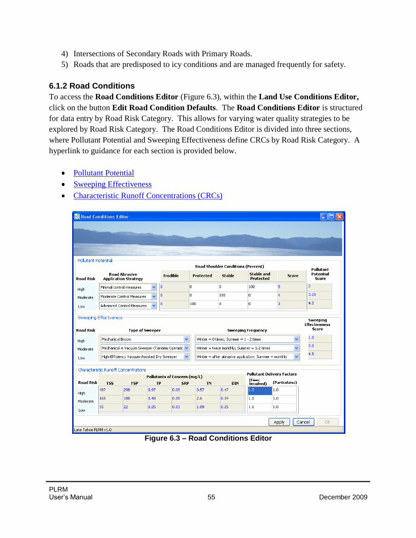
PLRM User’s Manual 55 December 2009
4) Intersections of Secondary Roads with Primary Roads.
5) Roads that are predisposed to icy conditions and are managed frequently for safety.
6.1.2 Road Conditions
To access the Road Conditions Editor (Figure 6.3), within the Land Use Conditions Editor,
click on the button Edit Road Condition Defaults. The Road Conditions Editor is structured
for data entry by Road Risk Category. This allows for varying water quality strategies to be
explored by Road Risk Category. The Road Conditions Editor is divided into three sections,
where Pollutant Potential and Sweeping Effectiveness define CRCs by Road Risk Category. A
hyperlink to guidance for each section is provided below.
Pollutant Potential
Sweeping Effectiveness
Characteristic Runoff Concentrations (CRCs)
Figure 6.3 – Road Conditions Editor
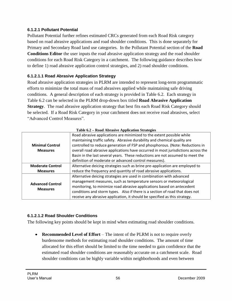
PLRM User’s Manual 56 December 2009
6.1.2.1 Pollutant Potential
Pollutant Potential further refines estimated CRCs generated from each Road Risk category
based on road abrasive applications and road shoulder conditions. This is done separately for
Primary and Secondary Road land use categories. In the Pollutant Potential section of the Road
Conditions Editor the user inputs the road abrasive application strategy and the road shoulder
conditions for each Road Risk Category in a catchment. The following guidance describes how
to define 1) road abrasive application control strategies, and 2) road shoulder conditions.
6.1.2.1.1 Road Abrasive Application Strategy
Road abrasive application strategies in PLRM are intended to represent long-term programmatic
efforts to minimize the total mass of road abrasives applied while maintaining safe driving
conditions. A general description of each strategy is provided in Table 6.2. Each strategy in
Table 6.2 can be selected in the PLRM drop-down box titled Road Abrasive Application
Strategy. The road abrasive application strategy that best fits each Road Risk Category should
be selected. If a Road Risk Category in your catchment does not receive road abrasives, select
“Advanced Control Measures”.
Table 6.2 – Road Abrasive Application Strategies
Minimal Control Measures
Road abrasive applications are minimized to the extent possible while maintaining traffic safety. Abrasive durability and chemical quality are controlled to reduce generation of FSP and phosphorous. (Note: Reductions in overall road abrasive applications have occurred in most jurisdictions across the Basin in the last several years. These reductions are not assumed to meet the definition of moderate or advanced control measures).
Moderate Control Measures
Alternative deicing strategies such as brine pre-application are employed to reduce the frequency and quantity of road abrasive applications.
Advanced Control Measures
Alternative deicing strategies are used in combination with advanced management measures, such as temperature sensors or meteorological monitoring, to minimize road abrasive applications based on antecedent conditions and storm types. Also if there is a section of road that does not receive any abrasive application, it should be specified as this strategy.
6.1.2.1.2 Road Shoulder Conditions
The following key points should be kept in mind when estimating road shoulder conditions.
Recommended Level of Effort – The intent of the PLRM is not to require overly
burdensome methods for estimating road shoulder conditions. The amount of time
allocated for this effort should be limited to the time needed to gain confidence that the
estimated road shoulder conditions are reasonably accurate on a catchment scale. Road
shoulder conditions can be highly variable within neighborhoods and even between
PLRM User’s Manual 57 December 2009
individual houses. Determining road shoulder condition is somewhat subjective. The
recommended level of effort for the Road Methodology is to designate the dominant
road shoulder condition by block (i.e. one designation for every 500 foot segment of
road). In many cases, the left and right road shoulder conditions may vary markedly for
the same block. If this occurs, the user should define the dominant road shoulder
condition for the left and right shoulder of the same block. The user can choose to define
road condition at a finer or coarser scale of spatial resolution if increased resolution is
thought to significantly improve results. In particular, the user may find it useful to
define a finer scale of spatial resolution for High Risk and Moderate Risk road shoulders
because these Road Risk Categories will likely have highest pollutant loads and therefore
will be targeted for water quality improvements.
Relationship to Impervious Area Connectivity – This section provides guidance on
estimating road shoulder condition as it relates to pollutant generation and PSC
implementation. As mentioned above, impervious area connectivity is not a
consideration for judging the condition of the road shoulder for pollutant generation. For
example, a disconnected compacted dirt road shoulder should not be defined as stable
because one might assume that storm water runoff does not reach a storm water inlet or
piping system. Using the PLRM methodology, a disconnected compacted dirt road
shoulder should be defined as erodible in the Road Conditions Editor and defined as
disconnected in the Drainage Conditions Editor (see Section 7). While pollutant
generation and impervious area connectivity are independent input parameters in the
PLRM, they are interdependent components of the pollutant load calculations in the
PLRM. Note that it will likely be more efficient to assess road shoulder condition and
impervious area connectivity of roads at the same time. Therefore, it is recommended
that the user review Section 7 of this manual before developing input parameters for road
shoulder conditions.
Guidance for Estimating Road Shoulder Conditions
The following is recommended guidance for populating the Road Shoulder Conditions table
within the Pollutant Potential section of the Road Conditions Editor. The necessary input for
the Road Conditions Editor is shown in Table 6.3. There are four types of road shoulder
conditions defined in the PLRM: 1) Erodible; 2) Protected; 3) Stable; and 4) Stable and
Protected. Within a catchment, the percentage of each road shoulder condition by Road Risk
Category must be tabulated, where the sum equals 100%.
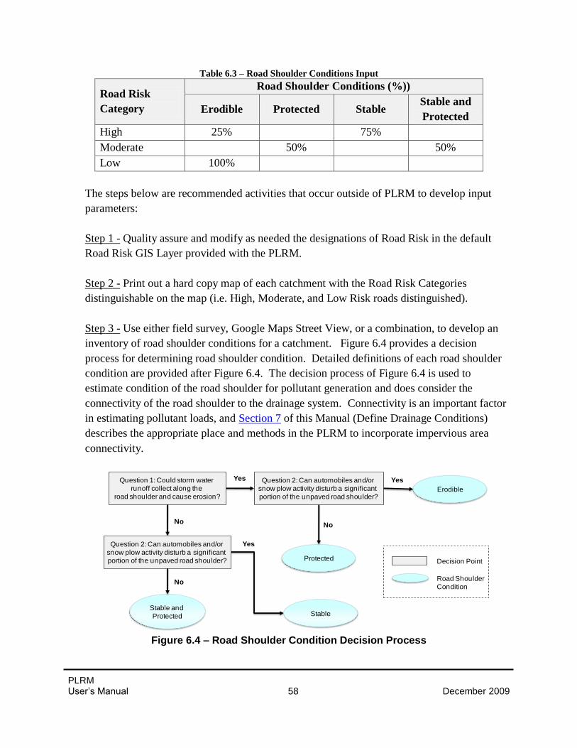
PLRM User’s Manual 58 December 2009
Table 6.3 – Road Shoulder Conditions Input
Road Risk
Category
Road Shoulder Conditions (%))
Erodible Protected Stable Stable and
Protected
High 25% 75%
Moderate 50% 50%
Low 100%
The steps below are recommended activities that occur outside of PLRM to develop input
parameters:
Step 1 - Quality assure and modify as needed the designations of Road Risk in the default
Road Risk GIS Layer provided with the PLRM.
Step 2 - Print out a hard copy map of each catchment with the Road Risk Categories
distinguishable on the map (i.e. High, Moderate, and Low Risk roads distinguished).
Step 3 - Use either field survey, Google Maps Street View, or a combination, to develop an
inventory of road shoulder conditions for a catchment. Figure 6.4 provides a decision
process for determining road shoulder condition. Detailed definitions of each road shoulder
condition are provided after Figure 6.4. The decision process of Figure 6.4 is used to
estimate condition of the road shoulder for pollutant generation and does consider the
connectivity of the road shoulder to the drainage system. Connectivity is an important factor
in estimating pollutant loads, and Section 7 of this Manual (Define Drainage Conditions)
describes the appropriate place and methods in the PLRM to incorporate impervious area
connectivity.
Figure 6.4 – Road Shoulder Condition Decision Process
Question 1: Could storm water
runoff collect along the
road shoulder and cause erosion?Erodible
Protected
Stable and
Protected
Yes
No
Road Shoulder
Condition
Decision Point
Question 2: Can automobiles and/or
snow plow activity disturb a significant
portion of the unpaved road shoulder?
Yes
No
No
Stable
Question 2: Can automobiles and/or
snow plow activity disturb a significant
portion of the unpaved road shoulder?
Yes
PLRM User’s Manual 59 December 2009
Mark-up the hard copy map with the dominant road shoulder condition by block, or your
preferred spatial resolution, using a color-coded legend. Distinguish between left and right
road shoulder conditions if they are markedly different on the same block.
Step 4 – For each Road Risk category in the catchment, estimate the percentage of area that
equates to a particular road shoulder condition. The percentage of area can be estimated by
transferring the hard copy map information to GIS or AutoCAD and tabulating distances by
Road Risk Category. Transferring the information to digital form will also allow for better
presentation and subsequent use in alternatives evaluation.
The estimate of road shoulder condition does not need to be precise. The intent of the Road
Methodology is to reasonably estimate the general distribution of road shoulder conditions
(e.g., Are the road shoulders 0%, 25%, 50%, 75%, or 100% stable?). Users may deviate
from these recommended steps based on available resources and compatibility with other
planning and maintenance activities – the key objectives are 1) categorization of road
segments at a reasonable resolution and 2) production of a digital record for use in model
input and analysis.
Definitions of Road Shoulder Condition
1. Stable – The road shoulders have physical improvements or other elements that either: 1)
promote sheet flow and avoid concentration of storm water and conveyance along the
road shoulder; or 2) stabilize the conveyance of storm water and inhibit erosion along the
road shoulder. Physical improvements are actions that stabilize a road shoulder (e.g.,
curb and gutter, rock-lined channel, etc.). Other elements can include vegetation that
stabilizes a road shoulder, or topography that promotes sheet flow and avoids
concentration and conveyance of storm water in the road shoulder. The following are
key points to consider when judging if a road shoulder is Stable.
a. Following the decision process of Figure 6.4, ask the question: Could storm water
runoff collect along the road shoulder and cause erosion?
i. If the answer is YES, then the road shoulder is not stable.
ii. If the answer is NO, then the road shoulder is stable.
b. Visual evidence of erosion in the road shoulder is not required to make a
determination that the road shoulder is not stable.
2. Protected – The road shoulders have physical features (e.g. structures, vegetation, etc) or
policies (parking ordinances) that discourage or minimize disturbance by automobiles
and snow plows. Defining a road shoulder as Protected means that the majority of the
PLRM User’s Manual 60 December 2009
pervious portion of road shoulder within the public right-of-way will remain undisturbed
under typical conditions. The following are key points and definitions to consider when
judging if a road shoulder is protected.
a. “Typical condition” is defined as a state that can be reasonably anticipated. For
example, the presence of vegetation in the road shoulder is not much of a barrier
to a snow plow, but the presence of vegetation indicates that under “typical
conditions” the shoulder is not disturbed by plowing and therefore can be
considered Protected.
b. Following the decision process of Figure 6.4, ask the question: Can automobiles
and/or snow plow activity disturb a significant portion of the unpaved road
shoulder?
i. If the answer is YES, then the road shoulder is not protected.
ii. If the answer is NO, then the road shoulder is protected.
c. In cases where a policy is implemented to discourage road shoulder disturbance,
the user may need to judge the success of the policy by estimating the amount of
visual disturbance in the road shoulder. For example, if 20% of the road
shoulders within a particular block appear to be parked on, then the parking
ordinance is protecting 80% of the road shoulders on the block.
3. Stable and Protected – The road shoulders meet the definitions of stable and protected
as discussed above. Following the decision process of Figure 6.4, the answer to the
following two questions would be NO:
a. Could storm water runoff collect along the road shoulder and cause erosion?
b. Can automobiles and/or snow plow activity disturb a significant portion of the
unpaved road shoulder?
4. Erodible – The road shoulders do not meet the definitions of stable or protected as
discussed above. Following the decision process of Figure 6.4, the answer to the
following two questions would be YES:
a. Could storm water runoff collect along the road shoulder and cause erosion?
b. Can automobiles and/or snow plow activity disturb a significant portion of the
unpaved road shoulder?
PLRM User’s Manual 61 December 2009
Developing Road Shoulder Conditions for Formulated Alternatives
The methods in the PLRM do not explicitly distinguish or rank the different types of PSCs that
could be implemented on road shoulders. It is up to the project designer and project reviewers to
assess how proposed PSCs in formulated alternatives will influence the condition of road
shoulders in terms of pollutant generation. Water quality improvements attributed to PSC
implementation on road shoulders is based on the road shoulder condition they create. Any PSC
that creates the same road shoulder condition is considered equal in the methodology in terms of
pollutant generation. For example, the Road Methodology does not distinguish between curb
and gutter and a rock-lined channel. Using the PLRM definitions for road shoulder condition,
both curb and gutter and a rock-lined channel are PSCs that could create a stabilized road
shoulder condition. However, user discretion should be applied to adjust road shoulder
conditions as deemed appropriate. For example, if an existing rock-lined channel was not
deemed to be effective at stabilizing a road shoulder, then the user could classify that particular
road shoulder as “not stable”.
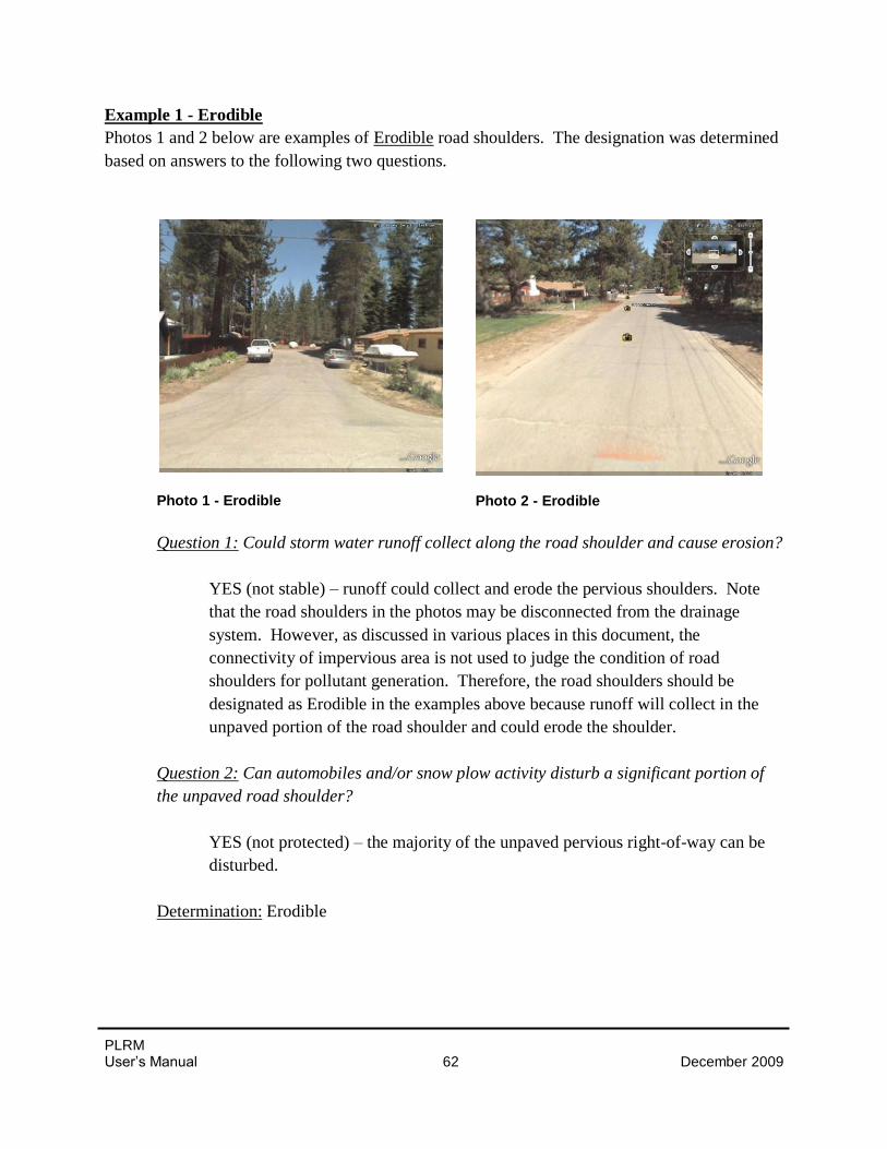
PLRM User’s Manual 62 December 2009
Example 1 - Erodible
Photos 1 and 2 below are examples of Erodible road shoulders. The designation was determined
based on answers to the following two questions.
Photo 1 - Erodible
Question 1: Could storm water runoff collect along the road shoulder and cause erosion?
YES (not stable) – runoff could collect and erode the pervious shoulders. Note
that the road shoulders in the photos may be disconnected from the drainage
system. However, as discussed in various places in this document, the
connectivity of impervious area is not used to judge the condition of road
shoulders for pollutant generation. Therefore, the road shoulders should be
designated as Erodible in the examples above because runoff will collect in the
unpaved portion of the road shoulder and could erode the shoulder.
Question 2: Can automobiles and/or snow plow activity disturb a significant portion of
the unpaved road shoulder?
YES (not protected) – the majority of the unpaved pervious right-of-way can be
disturbed.
Determination: Erodible
Photo 2 - Erodible
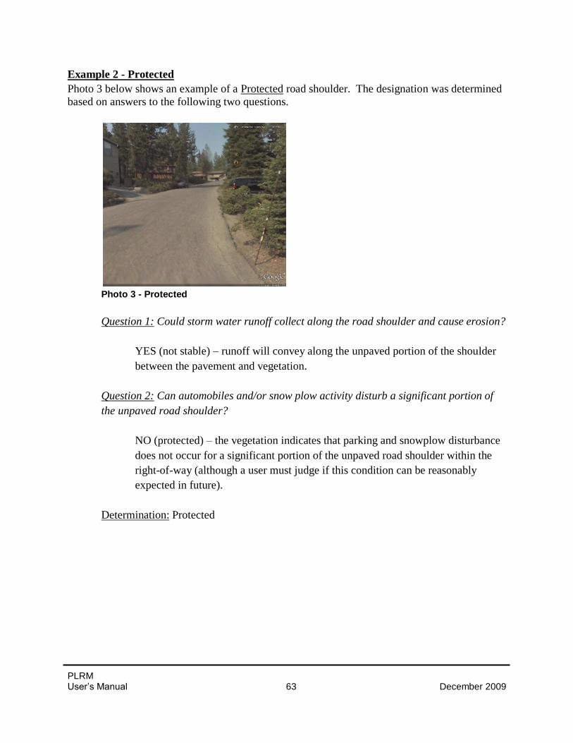
PLRM User’s Manual 63 December 2009
Example 2 - Protected
Photo 3 below shows an example of a Protected road shoulder. The designation was determined
based on answers to the following two questions.
Photo 3 - Protected
Question 1: Could storm water runoff collect along the road shoulder and cause erosion?
YES (not stable) – runoff will convey along the unpaved portion of the shoulder
between the pavement and vegetation.
Question 2: Can automobiles and/or snow plow activity disturb a significant portion of
the unpaved road shoulder?
NO (protected) – the vegetation indicates that parking and snowplow disturbance
does not occur for a significant portion of the unpaved road shoulder within the
right-of-way (although a user must judge if this condition can be reasonably
expected in future).
Determination: Protected
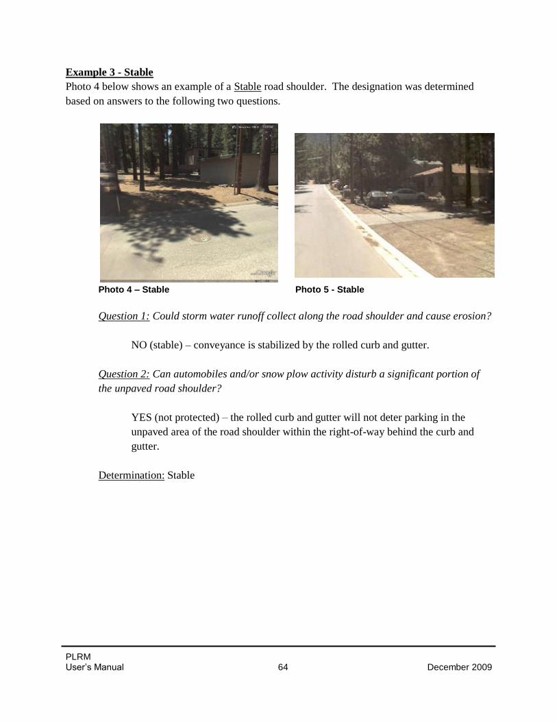
PLRM User’s Manual 64 December 2009
Example 3 - Stable
Photo 4 below shows an example of a Stable road shoulder. The designation was determined
based on answers to the following two questions.
Photo 4 – Stable Photo 5 - Stable
Question 1: Could storm water runoff collect along the road shoulder and cause erosion?
NO (stable) – conveyance is stabilized by the rolled curb and gutter.
Question 2: Can automobiles and/or snow plow activity disturb a significant portion of
the unpaved road shoulder?
YES (not protected) – the rolled curb and gutter will not deter parking in the
unpaved area of the road shoulder within the right-of-way behind the curb and
gutter.
Determination: Stable
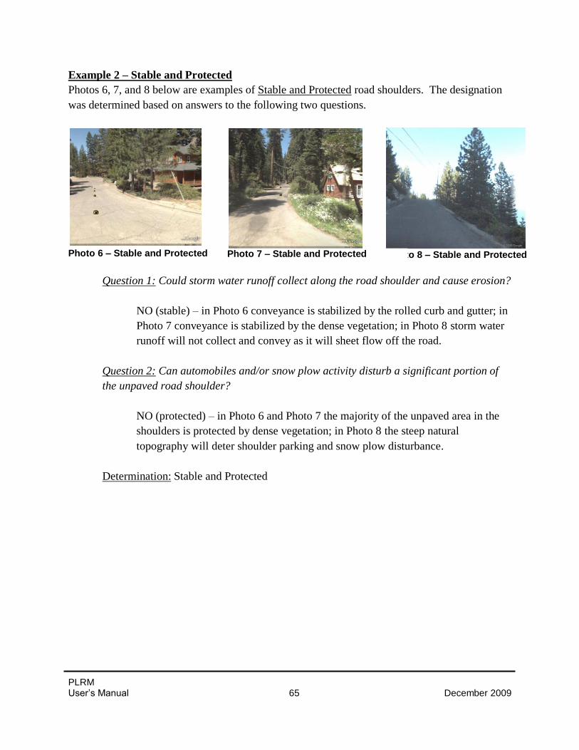
PLRM User’s Manual 65 December 2009
Example 2 – Stable and Protected
Photos 6, 7, and 8 below are examples of Stable and Protected road shoulders. The designation
was determined based on answers to the following two questions.
Photo 6 – Stable and Protected
Question 1: Could storm water runoff collect along the road shoulder and cause erosion?
NO (stable) – in Photo 6 conveyance is stabilized by the rolled curb and gutter; in
Photo 7 conveyance is stabilized by the dense vegetation; in Photo 8 storm water
runoff will not collect and convey as it will sheet flow off the road.
Question 2: Can automobiles and/or snow plow activity disturb a significant portion of
the unpaved road shoulder?
NO (protected) – in Photo 6 and Photo 7 the majority of the unpaved area in the
shoulders is protected by dense vegetation; in Photo 8 the steep natural
topography will deter shoulder parking and snow plow disturbance.
Determination: Stable and Protected
Photo 8 – Stable and Protected
Photo 7 – Stable and Protected
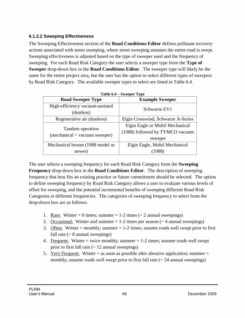
PLRM User’s Manual 66 December 2009
6.1.2.2 Sweeping Effectiveness
The Sweeping Effectiveness section of the Road Conditions Editor defines pollutant recovery
actions associated with street sweeping, where street sweeping assumes the entire road is swept.
Sweeping effectiveness is adjusted based on the type of sweeper used and the frequency of
sweeping. For each Road Risk Category the user selects a sweeper type from the Type of
Sweeper drop-down box in the Road Conditions Editor. The sweeper type will likely be the
same for the entire project area, but the user has the option to select different types of sweepers
by Road Risk Category. The available sweeper types to select are listed in Table 6.4.
Table 6.4 – Sweeper Type
Road Sweeper Type Example Sweeper
High-efficiency vacuum-assisted
(dustless) Schwarze EV1
Regenerative air (dustless) Elgin Crosswind, Schwarze A-Series
Tandem operation
(mechanical + vacuum sweeper)
Elgin Eagle or Mobil Mechanical
(1988) followed by TYMCO vacuum
sweeper
Mechanical broom (1988 model or
newer)
Elgin Eagle, Mobil Mechanical
(1988)
The user selects a sweeping frequency for each Road Risk Category from the Sweeping
Frequency drop-down box in the Road Conditions Editor. The description of sweeping
frequency that best fits an existing practice or future commitment should be selected. The option
to define sweeping frequency by Road Risk Category allows a user to evaluate various levels of
effort for sweeping, and the potential incremental benefits of sweeping different Road Risk
Categories at different frequencies. The categories of sweeping frequency to select from the
drop-down box are as follows:
1. Rare: Winter = 0 times; summer = 1-2 times (~ 2 annual sweepings)
2. Occasional: Winter and summer = 1-2 times per season (~ 4 annual sweepings)
3. Often: Winter = monthly; summer = 1-2 times; assume roads well swept prior to first
fall rain (~ 8 annual sweepings)
4. Frequent: Winter = twice monthly; summer = 1-2 times; assume roads well swept
prior to first fall rain (~ 12 annual sweepings)
5. Very Frequent: Winter = as soon as possible after abrasive application; summer =
monthly; assume roads well swept prior to first fall rain (~ 24 annual sweepings)
PLRM User’s Manual 67 December 2009
6.1.2.3 Characteristic Runoff Concentrations (CRCs)
The condition of roads within a catchment is correlated to characteristic runoff concentrations
(CRCs) to estimate average pollutant generation. A CRC is a representative concentration for a
pollutant of concern in runoff from a specific Road Land Use, Road Risk Category, and
associated condition. When combined with continuous runoff hydrology from the
PLRM, CRCs are intended to provide a representative estimate of average annual pollutant
loading for specific land use conditions.
CRCs are automatically calculated within the Road Conditions Editor for each Road Risk
Category as information is entered for Pollutant Potential and Sweeping Effectiveness. CRCs
are calculated for all pollutants of concern, which include:
TSS – Total Suspended Sediment
FSP – Fine Sediment Particles (TSS less than 16 microns in diameter)
TP – Total Phosphorus
SRP – Soluble Reactive Phosphorus
TN – Total Nitrogen
DIN – Dissolved Inorganic Nitrogen
The research and development that went in to relating Pollutant Potential and Sweeping
Effectiveness to CRCs for each pollutant of concern can be reviewed in the Model Development
Document in Section 5, Appendix A, and Appendix B.
Pollutant Delivery Factors
Pollutant Delivery Factors provide a method to adjust the quantity of pollutants of concern
delivered to the outlet of the catchment. This option was included in the Road Conditions
Editor recognizing that the Road Methodology does not account for every PSC action that may
be implemented to improve the quality of runoff generated from roads. The intent of Pollutant
Delivery Factors is to provide a flexible and transparent process for adjusting pollutant loads if
the Road Methodology is deemed insufficient for representing PSCs.
By default, Pollutant Delivery Factors are set to 1 in the Road Conditions Editor. Changing a
Pollutant Delivery Factor to a value other than 1 will linearly adjust CRCs for pollutants of
concern. Two Pollutant Delivery Factors are provided to separately adjust 1) Particulate CRCs
= TSS, TP, and TN, and 2) Fines and Dissolved CRCs = FSP, SRP, and DIN. Adjusting
Pollutant Delivery Factors to a value other than 1 is acceptable, but the adjustment will be
flagged by the Recommended Range Report because the user should provide justification to
project reviewers when Pollutant Delivery Factors other than 1 are used.
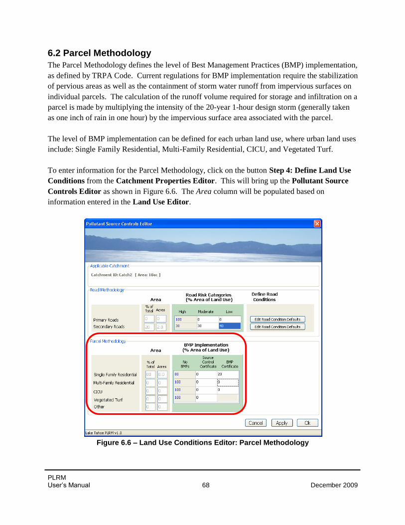
PLRM User’s Manual 68 December 2009
6.2 Parcel Methodology
The Parcel Methodology defines the level of Best Management Practices (BMP) implementation,
as defined by TRPA Code. Current regulations for BMP implementation require the stabilization
of pervious areas as well as the containment of storm water runoff from impervious surfaces on
individual parcels. The calculation of the runoff volume required for storage and infiltration on a
parcel is made by multiplying the intensity of the 20-year 1-hour design storm (generally taken
as one inch of rain in one hour) by the impervious surface area associated with the parcel.
The level of BMP implementation can be defined for each urban land use, where urban land uses
include: Single Family Residential, Multi-Family Residential, CICU, and Vegetated Turf.
To enter information for the Parcel Methodology, click on the button Step 4: Define Land Use
Conditions from the Catchment Properties Editor. This will bring up the Pollutant Source
Controls Editor as shown in Figure 6.6. The Area column will be populated based on
information entered in the Land Use Editor.
Figure 6.6 – Land Use Conditions Editor: Parcel Methodology
PLRM User’s Manual 69 December 2009
Note that the current version of the form will display all available urban land uses in the PLRM,
but the Area for land uses that are not defined to be present in the Land Use Editor will be equal
to zero. While the form would allow entry of information for urban land uses not present in the
catchment, the program would not use the input.
BMP implementation is entered in the Pollutant Source Controls Editor by defining the
percent of area for each urban land use with completed BMPs. In typical practice, the amount of
BMP implementation is reported based on the number of parcels with completed BMPs. If data
is only available on the number of parcels with completed BMPs for existing conditions, this
data will need to be converted to an area using GIS or by assuming an average size for the
parcels.
There are two types of BMP Implementation that can be defined in the PLRM: Source Control
Certificates and BMP Retrofit Certificates. The definition of each, which is based on TRPA
definitions, is as follows:
Source Control Certificate – a property has completed PSC implementation (i.e. pervious
areas of the property are stabilized). However, the property has recognized constraints
that do not allow for HSC implementation to the typical standard (i.e. storage of runoff
from 20-year 1-hour storm on the property). In the PLRM, defining a property to have a
source control certificate reduces the CRCs generated from that property.
BMP Retrofit Certificate – a property has completed both PSC implementation (i.e.
pervious areas of the property are stabilized) and HSC implementation to the typical
standard (i.e. storage of runoff from 20-year 1-hour storm on the property).
Representation in the PLRM
Source Control Certificates and BMP Retrofit Certificates signify that PSC implementation has
been completed for a certain amount of a particular land use. The designation of a Source
Control Certificate or BMP Retrofit Certificate will adjust pollutant generation through
adjustments to CRCs (Table 6.5) to signify that PSCs have been implemented.
While it is recognized that urban land use condition will vary substantially and result in variable
CRCs, a detailed methodology characterizing parcel condition was not part of the scope of work
for PLRM Version 1. Unlike the Road Methodology, the Parcel Methodology uses static CRC
values that reflect the average condition of a land use based on the presence of PSC
implementation or the absence of PSC implementation. Table 6.5 displays the default CRCs
used by the PLRM and the data sources used to develop the CRCs. Table 6.5 is not displayed in
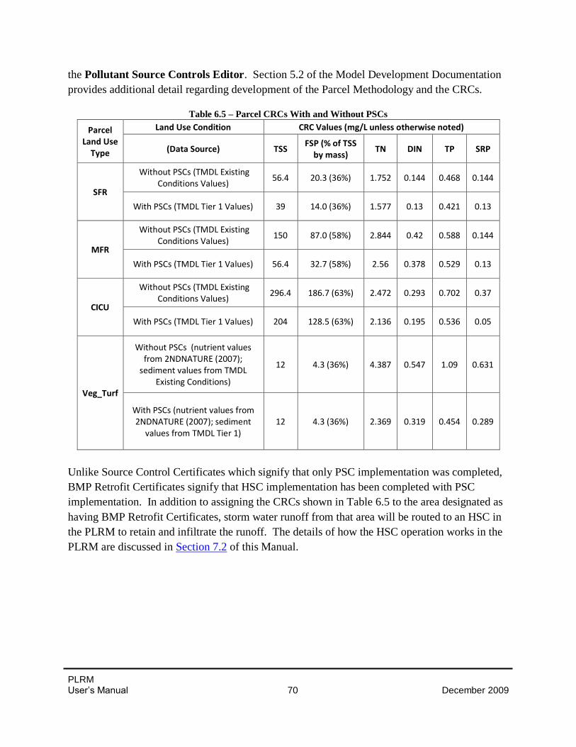
PLRM User’s Manual 70 December 2009
the Pollutant Source Controls Editor. Section 5.2 of the Model Development Documentation
provides additional detail regarding development of the Parcel Methodology and the CRCs.
Table 6.5 – Parcel CRCs With and Without PSCs
Parcel Land Use
Type
Land Use Condition CRC Values (mg/L unless otherwise noted)
(Data Source) TSS FSP (% of TSS
by mass) TN DIN TP SRP
SFR
Without PSCs (TMDL Existing Conditions Values)
56.4 20.3 (36%) 1.752 0.144 0.468 0.144
With PSCs (TMDL Tier 1 Values) 39 14.0 (36%) 1.577 0.13 0.421 0.13
MFR
Without PSCs (TMDL Existing Conditions Values)
150 87.0 (58%) 2.844 0.42 0.588 0.144
With PSCs (TMDL Tier 1 Values) 56.4 32.7 (58%) 2.56 0.378 0.529 0.13
CICU
Without PSCs (TMDL Existing Conditions Values)
296.4 186.7 (63%) 2.472 0.293 0.702 0.37
With PSCs (TMDL Tier 1 Values) 204 128.5 (63%) 2.136 0.195 0.536 0.05
Veg_Turf
Without PSCs (nutrient values from 2NDNATURE (2007);
sediment values from TMDL Existing Conditions)
12 4.3 (36%) 4.387 0.547 1.09 0.631
With PSCs (nutrient values from 2NDNATURE (2007); sediment
values from TMDL Tier 1) 12 4.3 (36%) 2.369 0.319 0.454 0.289
Unlike Source Control Certificates which signify that only PSC implementation was completed,
BMP Retrofit Certificates signify that HSC implementation has been completed with PSC
implementation. In addition to assigning the CRCs shown in Table 6.5 to the area designated as
having BMP Retrofit Certificates, storm water runoff from that area will be routed to an HSC in
the PLRM to retain and infiltrate the runoff. The details of how the HSC operation works in the
PLRM are discussed in Section 7.2 of this Manual.
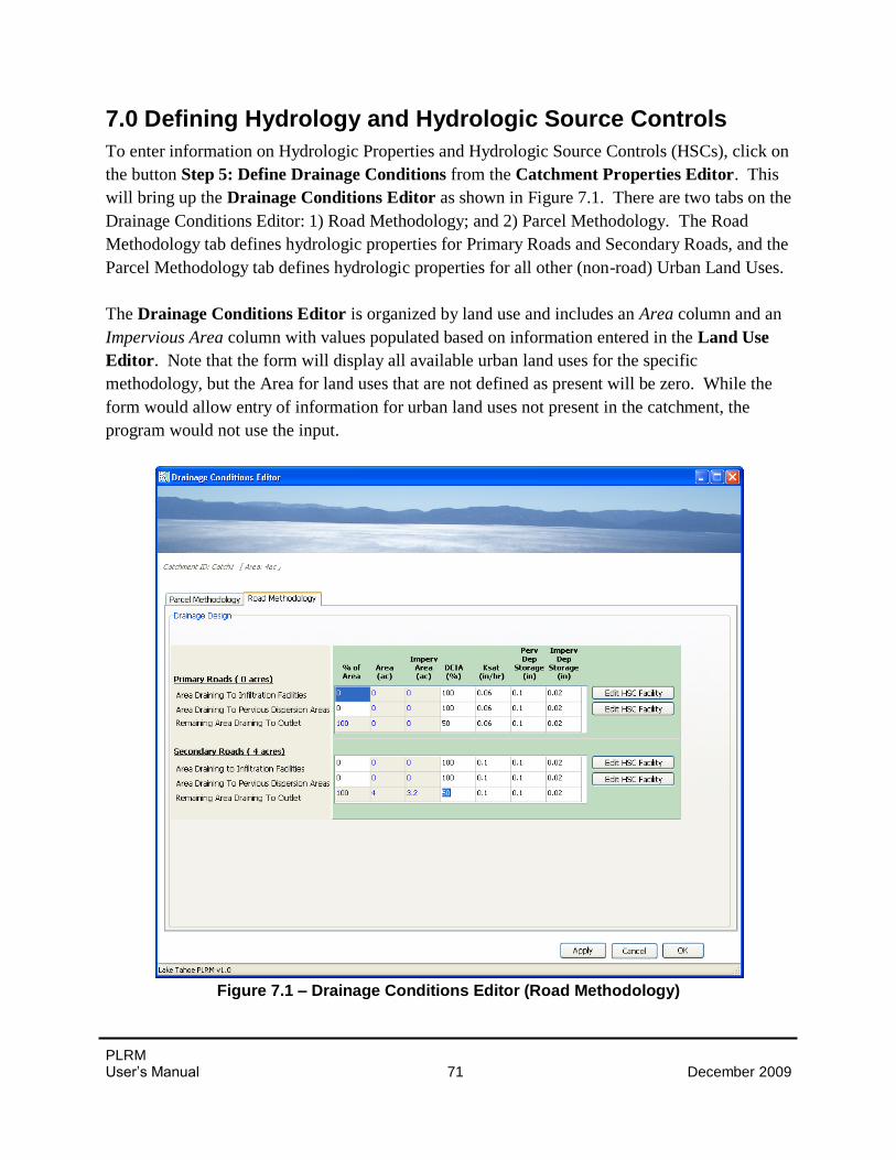
PLRM User’s Manual 71 December 2009
7.0 Defining Hydrology and Hydrologic Source Controls
To enter information on Hydrologic Properties and Hydrologic Source Controls (HSCs), click on
the button Step 5: Define Drainage Conditions from the Catchment Properties Editor. This
will bring up the Drainage Conditions Editor as shown in Figure 7.1. There are two tabs on the
Drainage Conditions Editor: 1) Road Methodology; and 2) Parcel Methodology. The Road
Methodology tab defines hydrologic properties for Primary Roads and Secondary Roads, and the
Parcel Methodology tab defines hydrologic properties for all other (non-road) Urban Land Uses.
The Drainage Conditions Editor is organized by land use and includes an Area column and an
Impervious Area column with values populated based on information entered in the Land Use
Editor. Note that the form will display all available urban land uses for the specific
methodology, but the Area for land uses that are not defined as present will be zero. While the
form would allow entry of information for urban land uses not present in the catchment, the
program would not use the input.
Figure 7.1 – Drainage Conditions Editor (Road Methodology)
PLRM User’s Manual 72 December 2009
In the PLRM, hydrologic calculations are aggregated by land use. This approach supports land –
use based pollutant load computations by facilitating hydrologic analysis by land use (e.g.,
routing a portion of the Secondary Roads to a pervious area or installation of private property
BMPs within residential land uses).
Note that land uses are typically distributed through a
catchment, and aggregation by land use does not allow
flows or loads to be tracked geographically within a
catchment – if results are needed for a particular portion
of a catchment, it should be divided into two or more
catchments. Additionally, if hydrologic properties of a
single land use are significantly different from one
portion of the catchment to another, it may be
advantageous to use two or more catchments.
In the Drainage Conditions Editor, the user is required
to enter the hydrologic properties that most strongly influence calculations of surface runoff in
the PLRM. The discussion in the following section describes entry of information in the PLRM
for a single catchment. This simplifies the text, but is not a limitation of the PLRM. There is no
limitation on the number of catchments that can be simulated in a Scenario in the PLRM.
Key Concept Box
Land uses are typically
distributed through a catchment,
and aggregation by land use does
not allow flows or loads to be
tracked geographically within a
catchment – if results are needed
for a particular portion of a
catchment, it should be divided
into two or more catchments.
PLRM User’s Manual 73 December 2009
7.1 Drainage Conditions
For each urban land use, Drainage conditions are defined by estimating the portions of a land use
routed to the catchment outlet or to an HSC facility; where an HSC facility can either be an
Infiltration Facility or a pervious area where storm water runoff is dispersed – termed a Pervious
Dispersion Area. Defining Drainage Conditions based on the routing of storm water for a
particular land use is termed Land Use Routing in the PLRM. Land Use Routing allows the
PLRM to account for flow volume reductions associated with Hydrologic Source Controls
(HSCs) implemented for a specific land use.
The methods used to define Drainage Conditions are not
intended to require a detailed tabulation in GIS or
AutoCAD. The user should estimate the general
characteristics by land use (e.g., does 0%, 25%, 50%, 75%,
or 100% of Secondary Roads within the catchment drain to
infiltration facilities?).
Road Methodology
For the Road Methodology, three types of Drainage
Conditions are defined for each Road Land Use (Primary
Roads and Secondary Roads). The user specifies the % of
Area in each Drainage Condition in the Drainage Conditions Editor. Drainage Conditions in
the Road Methodology are defined as follows:
Area Draining to Infiltration Facilities – the impervious portion of a road land use within
the catchment routed to an Infiltration Facility. An Infiltration Facility could be a dry
well, an infiltration trench, or any other physical structure designed to store and infiltrate
runoff.
Area Draining to Pervious Dispersion Areas – the impervious portion of a road land use
within the catchment routed to a pervious surface for dispersal and infiltration of runoff.
A Pervious Dispersion Area is typically not the pervious portion of the right-of-way, but
rather an urban lot, or collection of urban lots, where storm water is dispersed.
Representing impervious/pervious connectivity of the pervious portion of the right-of-
way is defined by specifying Directly Connected Impervious Area (DCIA), discussed in
Section 7.2 of this Manual.
Remaining Area Draining to the Outlet – the impervious portion of a road land use within
the catchment not routed to an HSC Facility prior to reaching the catchment outlet. An
HSC Facility is either an Infiltration Facility or a Pervious Dispersion Area.
Key Concept Box
The methods used to define
Drainage Conditoins are not
intended to require a detailed
tabulation in GIS or AutoCAD.
The intent of the methods is to
reasonably estimate the general
characteristics of storm water
routing within a catchment by
land use.
PLRM User’s Manual 74 December 2009
Parcel Methodology
The tab in the Parcel Methodology in the Drainage Conditions Editor is similar to the Road
Methodology except the Parcel Methodology does not include an option to specify a Drainage
Conditions for: Area Draining to Pervious Dispersion Areas. Representation of
impervious/pervious connectivity for urban land uses included in the Parcel Methodology is
defined by specifying Directly Connected Impervious Area (DCIA), discussed in Section 7.2 of
this Manual. Urban Land Uses in the Parcel Methodology include: Single Family Residential;
Multi-Family Residential; CICU; and Vegetated Turf. Drainage Conditions in the Parcel
Methodology are defined as follows:
Area Draining to Infiltration Facilities – the impervious portion of an urban land use
within the catchment routed to an Infiltration Facility. An Infiltration Facility could be a
dry well, an infiltration trench, or any other physical structure designed to store and
infiltrate runoff.
Remaining Area Draining to the Outlet – the impervious portion of an urban land use
within the catchment not routed to an Infiltration Facility prior to the catchment outlet.
In the Parcel Methodology, the PLRM automatically inputs the % of Area value for the Drainage
Conditions: Area Draining to Infiltration Facilities and Remaining Area Draining to Outlet.
This is automatically done for each land use based on user entered information in the Land Use
Conditions Editor for BMP Retrofit Certificates. By definition, a BMP Retrofit Certificate
indicates impervious area on a parcel that is routed to an Infiltration Facility. For each Urban
Land Use in the Parcel Methodology, the % of Area value that the user entered for BMP Retrofit
Certificates is therefore the value used in the Drainage Conditions Editor for the Drainage
Area: Area Draining to Infiltration Areas. The remaining area is automatically calculated by the
PLRM and input into the Drainage Area: Remaining Area Draining to Outlet.
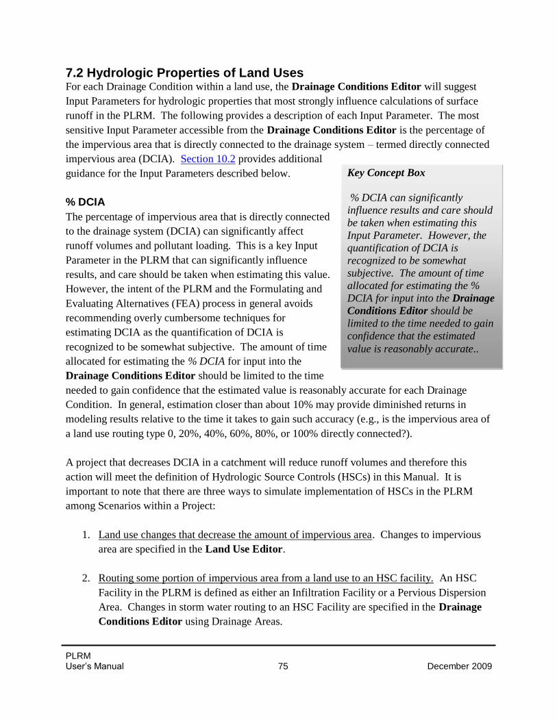
PLRM User’s Manual 75 December 2009
7.2 Hydrologic Properties of Land Uses For each Drainage Condition within a land use, the Drainage Conditions Editor will suggest
Input Parameters for hydrologic properties that most strongly influence calculations of surface
runoff in the PLRM. The following provides a description of each Input Parameter. The most
sensitive Input Parameter accessible from the Drainage Conditions Editor is the percentage of
the impervious area that is directly connected to the drainage system – termed directly connected
impervious area (DCIA). Section 10.2 provides additional
guidance for the Input Parameters described below.
% DCIA
The percentage of impervious area that is directly connected
to the drainage system (DCIA) can significantly affect
runoff volumes and pollutant loading. This is a key Input
Parameter in the PLRM that can significantly influence
results, and care should be taken when estimating this value.
However, the intent of the PLRM and the Formulating and
Evaluating Alternatives (FEA) process in general avoids
recommending overly cumbersome techniques for
estimating DCIA as the quantification of DCIA is
recognized to be somewhat subjective. The amount of time
allocated for estimating the % DCIA for input into the
Drainage Conditions Editor should be limited to the time
needed to gain confidence that the estimated value is reasonably accurate for each Drainage
Condition. In general, estimation closer than about 10% may provide diminished returns in
modeling results relative to the time it takes to gain such accuracy (e.g., is the impervious area of
a land use routing type 0, 20%, 40%, 60%, 80%, or 100% directly connected?).
A project that decreases DCIA in a catchment will reduce runoff volumes and therefore this
action will meet the definition of Hydrologic Source Controls (HSCs) in this Manual. It is
important to note that there are three ways to simulate implementation of HSCs in the PLRM
among Scenarios within a Project:
1. Land use changes that decrease the amount of impervious area. Changes to impervious
area are specified in the Land Use Editor.
2. Routing some portion of impervious area from a land use to an HSC facility. An HSC
Facility in the PLRM is defined as either an Infiltration Facility or a Pervious Dispersion
Area. Changes in storm water routing to an HSC Facility are specified in the Drainage
Conditions Editor using Drainage Areas.
Key Concept Box
% DCIA can significantly
influence results and care should
be taken when estimating this
Input Parameter. However, the
quantification of DCIA is
recognized to be somewhat
subjective. The amount of time
allocated for estimating the %
DCIA for input into the Drainage
Conditions Editor should be
limited to the time needed to gain
confidence that the estimated
value is reasonably accurate..
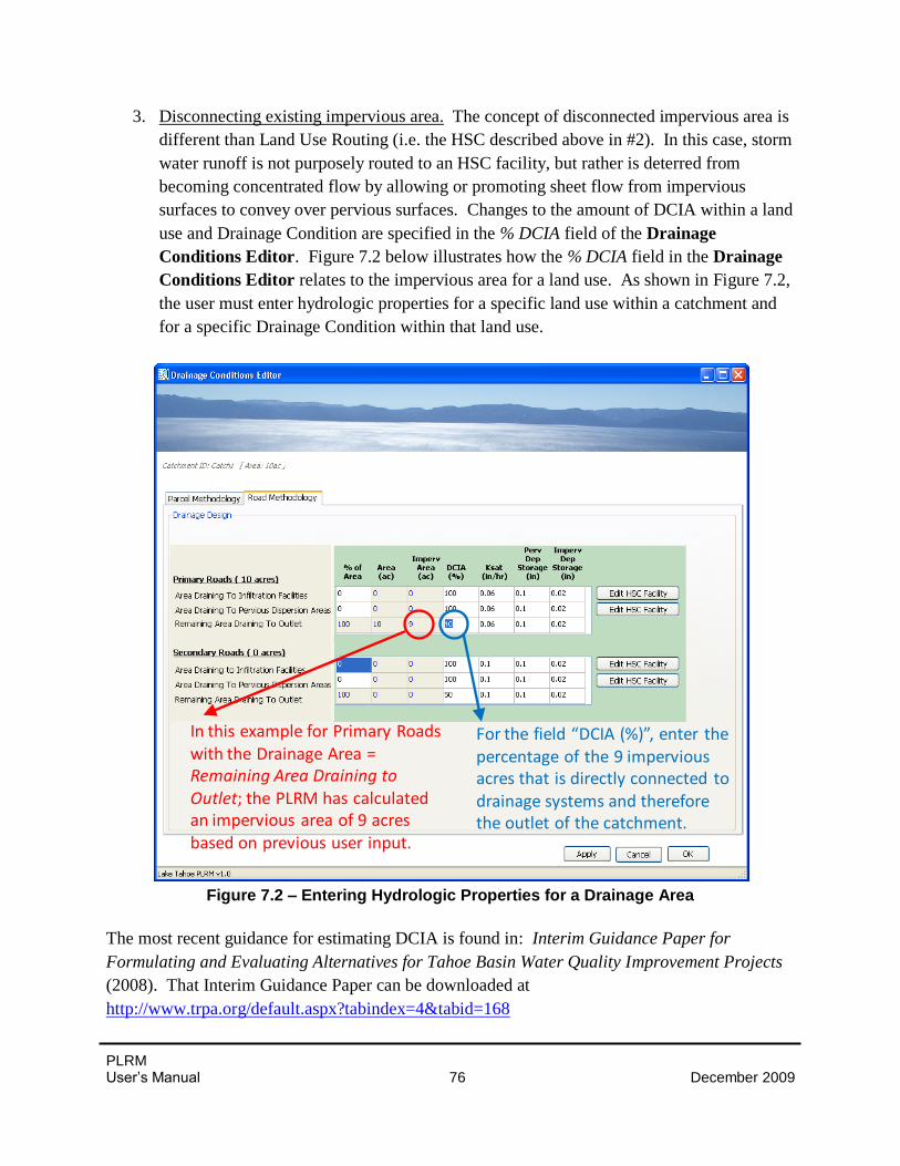
PLRM User’s Manual 76 December 2009
3. Disconnecting existing impervious area. The concept of disconnected impervious area is
different than Land Use Routing (i.e. the HSC described above in #2). In this case, storm
water runoff is not purposely routed to an HSC facility, but rather is deterred from
becoming concentrated flow by allowing or promoting sheet flow from impervious
surfaces to convey over pervious surfaces. Changes to the amount of DCIA within a land
use and Drainage Condition are specified in the % DCIA field of the Drainage
Conditions Editor. Figure 7.2 below illustrates how the % DCIA field in the Drainage
Conditions Editor relates to the impervious area for a land use. As shown in Figure 7.2,
the user must enter hydrologic properties for a specific land use within a catchment and
for a specific Drainage Condition within that land use.
Figure 7.2 – Entering Hydrologic Properties for a Drainage Area
The most recent guidance for estimating DCIA is found in: Interim Guidance Paper for
Formulating and Evaluating Alternatives for Tahoe Basin Water Quality Improvement Projects
(2008). That Interim Guidance Paper can be downloaded at
http://www.trpa.org/default.aspx?tabindex=4&tabid=168
In this example for Primary Roads with the Drainage Area = Remaining Area Draining to Outlet; the PLRM has calculated an impervious area of 9 acres based on previous user input.
For the field “DCIA (%)”, enter the percentage of the 9 impervious acres that is directly connected to drainage systems and therefore the outlet of the catchment.
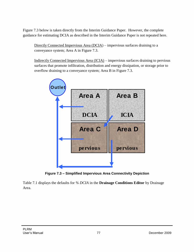
PLRM User’s Manual 77 December 2009
Figure 7.3 below is taken directly from the Interim Guidance Paper. However, the complete
guidance for estimating DCIA as described in the Interim Guidance Paper is not repeated here.
Directly Connected Impervious Area (DCIA) – impervious surfaces draining to a
conveyance system; Area A in Figure 7.3.
Indirectly Connected Impervious Area (ICIA) – impervious surfaces draining to pervious
surfaces that promote infiltration, distribution and energy dissipation, or storage prior to
overflow draining to a conveyance system; Area B in Figure 7.3.
Figure 7.3 – Simplified Impervious Area Connectivity Depiction
Table 7.1 displays the defaults for % DCIA in the Drainage Conditions Editor by Drainage
Area.
Area A
DCIA
Area B
ICIA
Area D
pervious
Area C
pervious
Outlet
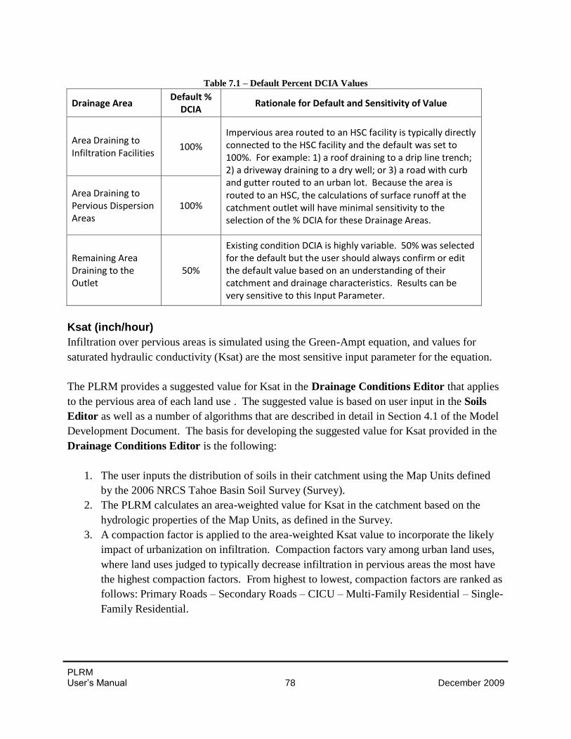
PLRM User’s Manual 78 December 2009
Table 7.1 – Default Percent DCIA Values
Drainage Area Default %
DCIA Rationale for Default and Sensitivity of Value
Area Draining to Infiltration Facilities
100%
Impervious area routed to an HSC facility is typically directly connected to the HSC facility and the default was set to 100%. For example: 1) a roof draining to a drip line trench; 2) a driveway draining to a dry well; or 3) a road with curb and gutter routed to an urban lot. Because the area is routed to an HSC, the calculations of surface runoff at the catchment outlet will have minimal sensitivity to the selection of the % DCIA for these Drainage Areas.
Area Draining to Pervious Dispersion Areas
100%
Remaining Area Draining to the Outlet
50%
Existing condition DCIA is highly variable. 50% was selected for the default but the user should always confirm or edit the default value based on an understanding of their catchment and drainage characteristics. Results can be very sensitive to this Input Parameter.
Ksat (inch/hour)
Infiltration over pervious areas is simulated using the Green-Ampt equation, and values for
saturated hydraulic conductivity (Ksat) are the most sensitive input parameter for the equation.
The PLRM provides a suggested value for Ksat in the Drainage Conditions Editor that applies
to the pervious area of each land use . The suggested value is based on user input in the Soils
Editor as well as a number of algorithms that are described in detail in Section 4.1 of the Model
Development Document. The basis for developing the suggested value for Ksat provided in the
Drainage Conditions Editor is the following:
1. The user inputs the distribution of soils in their catchment using the Map Units defined
by the 2006 NRCS Tahoe Basin Soil Survey (Survey).
2. The PLRM calculates an area-weighted value for Ksat in the catchment based on the
hydrologic properties of the Map Units, as defined in the Survey.
3. A compaction factor is applied to the area-weighted Ksat value to incorporate the likely
impact of urbanization on infiltration. Compaction factors vary among urban land uses,
where land uses judged to typically decrease infiltration in pervious areas the most have
the highest compaction factors. From highest to lowest, compaction factors are ranked as
follows: Primary Roads – Secondary Roads – CICU – Multi-Family Residential – Single-
Family Residential.
PLRM User’s Manual 79 December 2009
The user may override the suggested value for Ksat for each urban land use or for a specific
Drainage Condition within a land use in the Drainage Conditions Editor. The user should base
adjustments to Ksat on site specific information that may have been collected during an Existing
Conditions Analysis or field reconnaissance, and ensure that it represents anticipated long-term
performance.
Pervious Depression Storage (inch)
Pervious depression storage accounts for the storage of precipitation on pervious surfaces caused
by ponding, surface wetting, and interception. The default value in the PLRM is 0.1 inches. A
value close to 0.1 should be used for pervious areas without significant vegetation or forest
cover. A value closer to 0.2 should be used for areas with thick vegetative cover or a forest litter
layer.
Impervious Depression Storage (inch)
Impervious depression storage accounts for the storage of precipitation on impervious surfaces
caused by ponding, surface wetting, and interception. The default value of 0.05 inches is
recommended for use without modification.
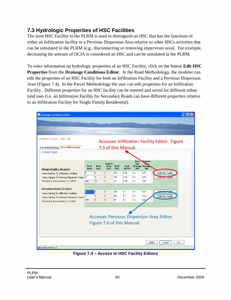
PLRM User’s Manual 80 December 2009
7.3 Hydrologic Properties of HSC Facilities The term HSC Facility in the PLRM is used to distinguish an HSC that has the functions of
either an Infiltration facility or a Pervious Dispersion Area relative to other HSCs activities that
can be simulated in the PLRM (e.g., disconnecting or removing impervious area). For example,
decreasing the amount of DCIA is considered an HSC and can be simulated in the PLRM.
To enter information on hydrologic properties of an HSC Facility, click on the button Edit HSC
Properties from the Drainage Conditions Editor. In the Road Methodology, the modeler can
edit the properties of an HSC Facility for both an Infiltration Facility and a Pervious Dispersion
Area (Figure 7.4). In the Parcel Methodology the user can edit properties for an Infiltration
Facility. Different properties for an HSC facility can be entered and saved for different urban
land uses (i.e. an Infiltration Facility for Secondary Roads can have different properties relative
to an Infiltration Facility for Single Family Residential).
Figure 7.4 – Access to HSC Facility Editors
Accesses Infiltration Facility Editor. Figure 7.5 of this Manual.
Accesses Pervious Dispersion Area Editor. Figure 7.6 of this Manual.
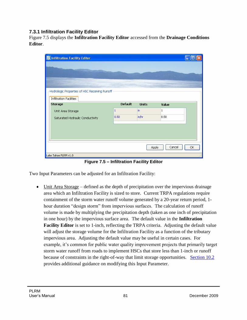
PLRM User’s Manual 81 December 2009
7.3.1 Infiltration Facility Editor Figure 7.5 displays the Infiltration Facility Editor accessed from the Drainage Conditions
Editor.
Figure 7.5 – Infiltration Facility Editor
Two Input Parameters can be adjusted for an Infiltration Facility:
Unit Area Storage – defined as the depth of precipitation over the impervious drainage
area which an Infiltration Facility is sized to store. Current TRPA regulations require
containment of the storm water runoff volume generated by a 20-year return period, 1-
hour duration “design storm” from impervious surfaces. The calculation of runoff
volume is made by multiplying the precipitation depth (taken as one inch of precipitation
in one hour) by the impervious surface area. The default value in the Infiltration
Facility Editor is set to 1-inch, reflecting the TRPA criteria. Adjusting the default value
will adjust the storage volume for the Infiltration Facility as a function of the tributary
impervious area. Adjusting the default value may be useful in certain cases. For
example, it’s common for public water quality improvement projects that primarily target
storm water runoff from roads to implement HSCs that store less than 1-inch or runoff
because of constraints in the right-of-way that limit storage opportunities. Section 10.2
provides additional guidance on modifying this Input Parameter.
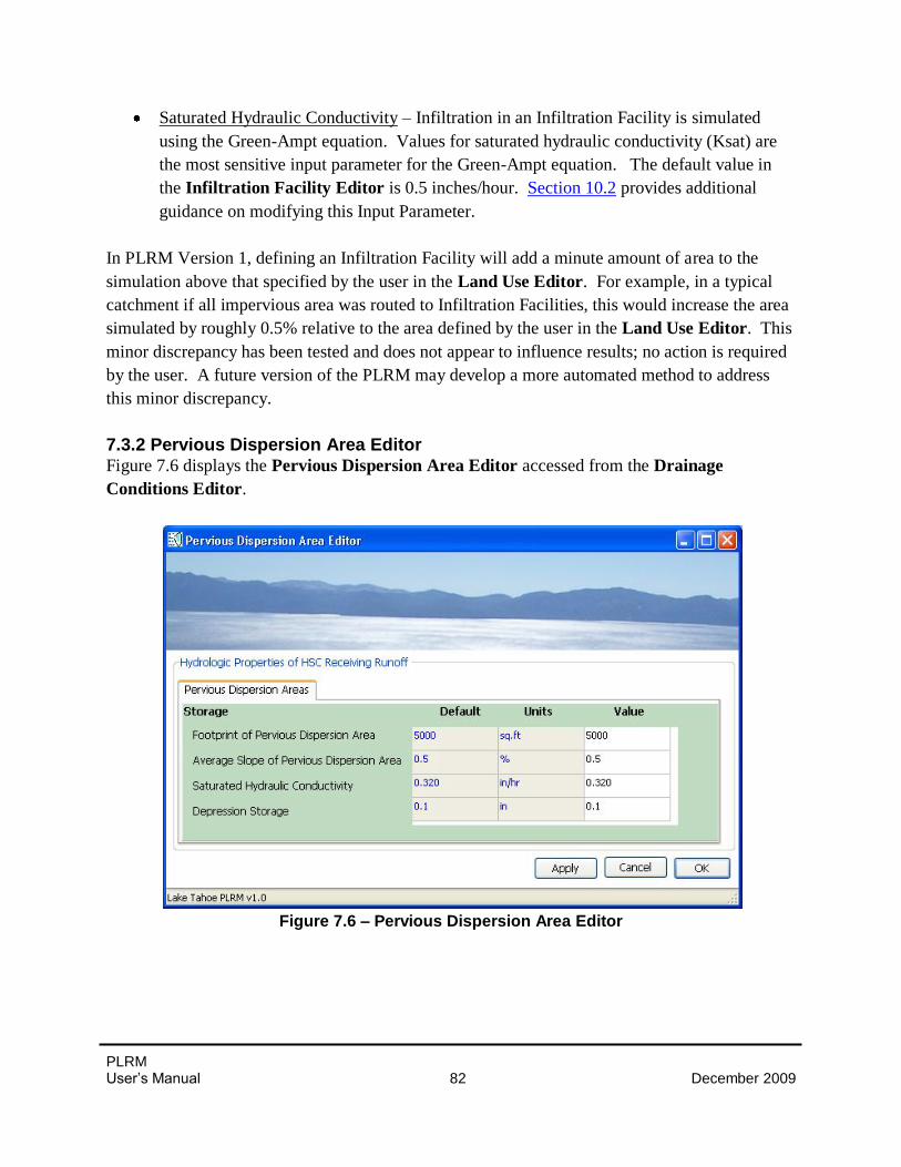
PLRM User’s Manual 82 December 2009
Saturated Hydraulic Conductivity – Infiltration in an Infiltration Facility is simulated
using the Green-Ampt equation. Values for saturated hydraulic conductivity (Ksat) are
the most sensitive input parameter for the Green-Ampt equation. The default value in
the Infiltration Facility Editor is 0.5 inches/hour. Section 10.2 provides additional
guidance on modifying this Input Parameter.
In PLRM Version 1, defining an Infiltration Facility will add a minute amount of area to the
simulation above that specified by the user in the Land Use Editor. For example, in a typical
catchment if all impervious area was routed to Infiltration Facilities, this would increase the area
simulated by roughly 0.5% relative to the area defined by the user in the Land Use Editor. This
minor discrepancy has been tested and does not appear to influence results; no action is required
by the user. A future version of the PLRM may develop a more automated method to address
this minor discrepancy.
7.3.2 Pervious Dispersion Area Editor Figure 7.6 displays the Pervious Dispersion Area Editor accessed from the Drainage
Conditions Editor.
Figure 7.6 – Pervious Dispersion Area Editor
PLRM User’s Manual 83 December 2009
Four Input Parameters can be adjusted for a Pervious Dispersion Area:
Footprint of Pervious Dispersion Area – the physical area of the Pervious Dispersion
Area that will typically be inundated with storm water. The default value is 5,000 square
feet, but the user should always adjust this value when modeling a Pervious Dispersion
Area dependent upon their site specific conditions and/or proposed project design.
Average Slope of Pervious Dispersion Area – average slope entered as a percent.
Saturated Hydraulic Conductivity – infiltration is simulated using the Green-Ampt
equation, and values for saturated hydraulic conductivity (Ksat) are the most sensitive
input parameter for the equation. The default value is 0.5 inches/hour. Section 10.2
provides additional guidance on this Input Parameter.
Depression Storage – Storage of precipitation provided through ponding, surface wetting,
and interception on pervious surfaces. Section 10.2 of this Manual provides guidance on
selecting a value for pervious depression storage based on the characteristics of the
pervious area. The default value for a Pervious Dispersion Area is 0.2 inches. A value
close to 0.1 should be used for pervious areas without significant vegetation or forest
cover. A value closer to 0.2 should be used for areas with thick vegetative cover or a
forest litter layer.
In PLRM Version 1, defining a Pervious Dispersion Area
will add area to the simulation above that specified by the
user in the Land Use Editor. Depending on the size of the
Pervious Dispersion Area, this could cause a notable
discrepancy in output. After adding a Pervious Dispersion
Area, the user should return to the Land Use Editor and
subtract out the area from the associated land use that
comprises the Pervious Dispersion Area. A future version
of the PLRM may develop a more automated method to
address this discrepancy.
Key Concept Box
A Pervious Dispersion Area will
add area above that specified by
the user in the Land Use Editor.
After adding a Pervious
Dispersion Area, the user should
return to the Land Use Editor
and subtract out the area from
the associated land use that
comprises the Pervious
Dispersion Area.
PLRM User’s Manual 84 December 2009
8.0 Defining Storm Water Treatment Facilities and Objects
There are a number of Storm Water Treatment (SWT) facilities than can be simulated in the
PLRM. A hyperlink to guidance describing each SWT, as well as the other PLRM objects
(junctions, outfalls, and dividers) is provided below. To use the hyperlink function, hold the
CTRL button on your keyboard and click on a hyperlink.
Dry Basins
Infiltration Basins
Wet Basins
Bed Filters
Cartridge Filters
Treatment Vaults or User-Defined SWT
Junctions, Outfalls, and Flow Dividers
The reduction in pollutant loading achieved by a SWT facility depends on the portion of runoff
treated and the extent of treatment achieved. The PLRM estimates pollutant load reductions
achieved by an SWT facility using basic design information supplied by the user and a long-term
simulation of hydrology to continuously compute hydraulic capture for the SWT. Runoff
captured by the SWT is considered treated, and is assigned a characteristic effluent concentration
(CEC) for pollutants of concern that is specific to each SWT facility. Runoff that is not captured
by the SWT is considered untreated or bypassed, and is assigned an effluent concentration
equaling the influent concentration. Pollutant loads can be reduced in a SWT facility through
reductions in storm water volumes and/or improvements in storm water quality. Both processes
are controlled by the hydraulic capture of the SWT (i.e. the percent of the runoff volume
captured and treated/removed by the SWT).
Depending on the type of SWT, there are several input parameters that influence the hydraulic
capture of an SWT, for example: storage volume, drain time, water quality flow rate, stage-
discharge relationships, and infiltration rate. The PLRM standardizes the representation of SWT
facilities and the required user supplied input parameters for each SWT that most strongly
influence hydraulic capture.
Water quality improvement attributed to the treatment of storm water in an SWT is modeled by
applying CECs to the volume of runoff captured that exits the treatment outlet of a SWT (if
present). If an influent concentration is less than a CEC for a pollutant of concern, then the CEC
will not be applied and effluent concentration equals influent concentration. Default values for
CECs are pre-loaded in the database for each SWT type. The current default CEC values are
based on best available data and were derived from statistical analysis of multiple storm water
PLRM User’s Manual 85 December 2009
performance studies to predict a representative level of treatment for each SWT facility for the
pollutants of concern. The PLRM Model Development Document (Section 7) provides
additional detail on how the default CECs were developed for each SWT facility.
As discussed in various places in this Manual, Input
Parameters should be characteristic of the long-term
average expected condition of the SWT. The PLRM will
simulate performance of an SWT continuously over an 18-
year time period when the Full Simulation option is
selected from the Project Editor. However, the Input
Parameters used to define the performance characteristics
of the SWT are static and do not explicitly account for
changes in condition over time, such as maintenance
activities or a lack of maintenance activities. Therefore, the
modeler must decide what the average expected condition
of the SWT will be for each Input Parameter required by
the PLRM over the life-span of the SWT, while factoring in
assumptions for anticipated or committed maintenance. Section 10.2 of this Manual provides
recommended ranges and guidance for key Input Parameters.
Key Concept Box
The PLRM will simulate
performance of an SWT
continuously over an 18-year
time period. However, the Input
Parameters used to define the
performance characteristics of
the SWT are static and do not
explicitly account for changes in
condition over time, such as
maintenance activities or a lack
of maintenance activities.
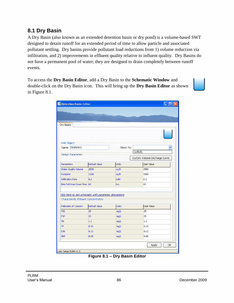
PLRM User’s Manual 86 December 2009
8.1 Dry Basin
A Dry Basin (also known as an extended detention basin or dry pond) is a volume-based SWT
designed to detain runoff for an extended period of time to allow particle and associated
pollutant settling. Dry basins provide pollutant load reductions from 1) volume reduction via
infiltration, and 2) improvements in effluent quality relative to influent quality. Dry Basins do
not have a permanent pool of water; they are designed to drain completely between runoff
events.
To access the Dry Basin Editor, add a Dry Basin to the Schematic Window and
double-click on the Dry Basin icon. This will bring up the Dry Basin Editor as shown
in Figure 8.1.
Figure 8.1 – Dry Basin Editor
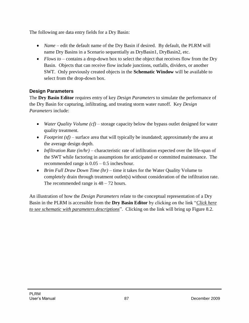
PLRM User’s Manual 87 December 2009
The following are data entry fields for a Dry Basin:
Name – edit the default name of the Dry Basin if desired. By default, the PLRM will
name Dry Basins in a Scenario sequentially as DryBasin1, DryBasin2, etc.
Flows to – contains a drop-down box to select the object that receives flow from the Dry
Basin. Objects that can receive flow include junctions, outfalls, dividers, or another
SWT. Only previously created objects in the Schematic Window will be available to
select from the drop-down box.
Design Parameters
The Dry Basin Editor requires entry of key Design Parameters to simulate the performance of
the Dry Basin for capturing, infiltrating, and treating storm water runoff. Key Design
Parameters include:
Water Quality Volume (cf) – storage capacity below the bypass outlet designed for water
quality treatment.
Footprint (sf) – surface area that will typically be inundated; approximately the area at
the average design depth.
Infiltration Rate (in/hr) – characteristic rate of infiltration expected over the life-span of
the SWT while factoring in assumptions for anticipated or committed maintenance. The
recommended range is 0.05 – 0.5 inches/hour.
Brim Full Draw Down Time (hr) – time it takes for the Water Quality Volume to
completely drain through treatment outlet(s) without consideration of the infiltration rate.
The recommended range is 48 – 72 hours.
An illustration of how the Design Parameters relate to the conceptual representation of a Dry
Basin in the PLRM is accessible from the Dry Basin Editor by clicking on the link “Click here
to see schematic with parameters descriptions”. Clicking on the link will bring up Figure 8.2.
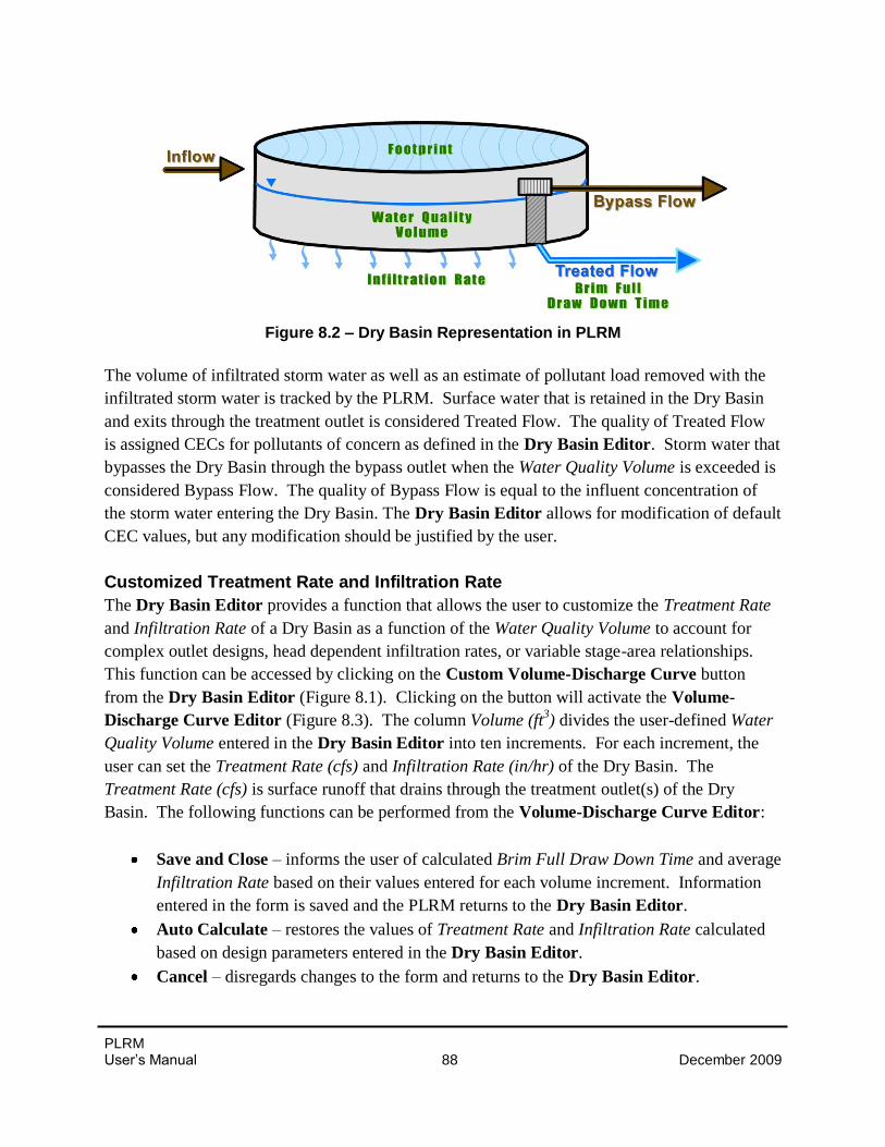
PLRM User’s Manual 88 December 2009
Figure 8.2 – Dry Basin Representation in PLRM
The volume of infiltrated storm water as well as an estimate of pollutant load removed with the
infiltrated storm water is tracked by the PLRM. Surface water that is retained in the Dry Basin
and exits through the treatment outlet is considered Treated Flow. The quality of Treated Flow
is assigned CECs for pollutants of concern as defined in the Dry Basin Editor. Storm water that
bypasses the Dry Basin through the bypass outlet when the Water Quality Volume is exceeded is
considered Bypass Flow. The quality of Bypass Flow is equal to the influent concentration of
the storm water entering the Dry Basin. The Dry Basin Editor allows for modification of default
CEC values, but any modification should be justified by the user.
Customized Treatment Rate and Infiltration Rate
The Dry Basin Editor provides a function that allows the user to customize the Treatment Rate
and Infiltration Rate of a Dry Basin as a function of the Water Quality Volume to account for
complex outlet designs, head dependent infiltration rates, or variable stage-area relationships.
This function can be accessed by clicking on the Custom Volume-Discharge Curve button
from the Dry Basin Editor (Figure 8.1). Clicking on the button will activate the Volume-
Discharge Curve Editor (Figure 8.3). The column Volume (ft3) divides the user-defined Water
Quality Volume entered in the Dry Basin Editor into ten increments. For each increment, the
user can set the Treatment Rate (cfs) and Infiltration Rate (in/hr) of the Dry Basin. The
Treatment Rate (cfs) is surface runoff that drains through the treatment outlet(s) of the Dry
Basin. The following functions can be performed from the Volume-Discharge Curve Editor:
Save and Close – informs the user of calculated Brim Full Draw Down Time and average
Infiltration Rate based on their values entered for each volume increment. Information
entered in the form is saved and the PLRM returns to the Dry Basin Editor.
Auto Calculate – restores the values of Treatment Rate and Infiltration Rate calculated
based on design parameters entered in the Dry Basin Editor.
Cancel – disregards changes to the form and returns to the Dry Basin Editor.
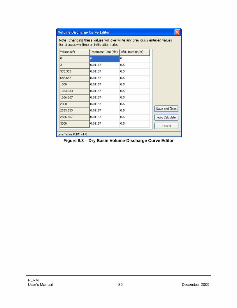
PLRM User’s Manual 89 December 2009
Figure 8.3 – Dry Basin Volume-Discharge Curve Editor
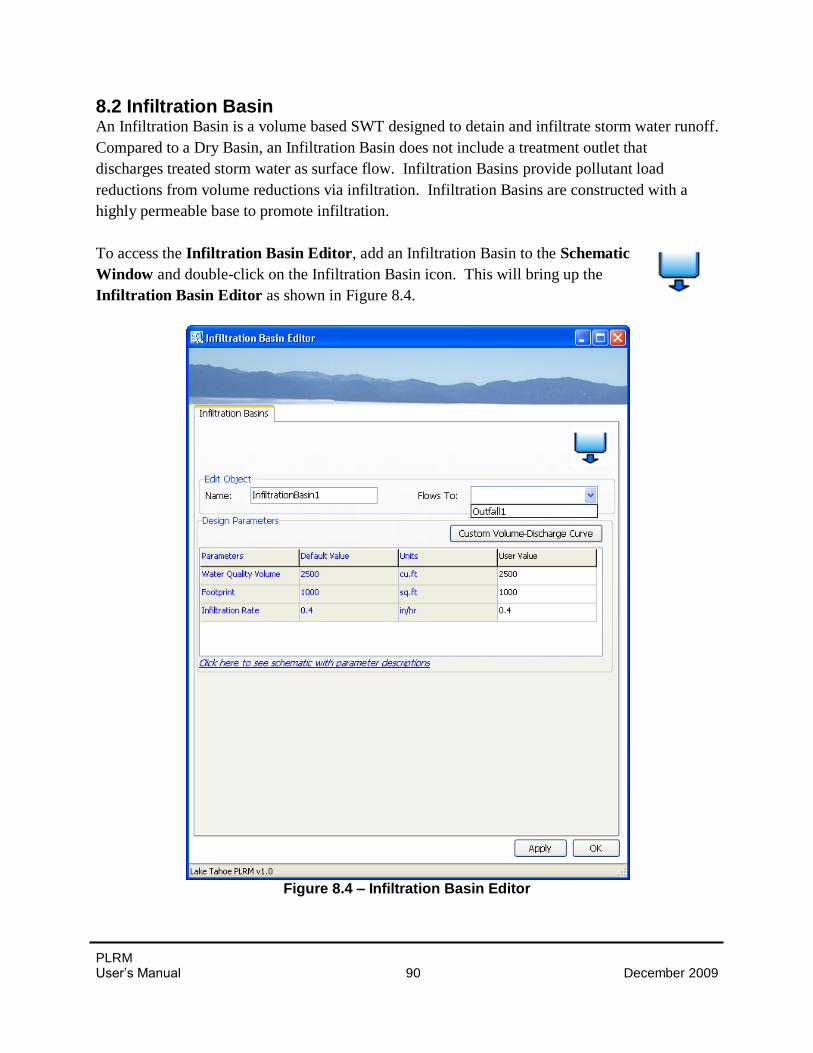
PLRM User’s Manual 90 December 2009
8.2 Infiltration Basin An Infiltration Basin is a volume based SWT designed to detain and infiltrate storm water runoff.
Compared to a Dry Basin, an Infiltration Basin does not include a treatment outlet that
discharges treated storm water as surface flow. Infiltration Basins provide pollutant load
reductions from volume reductions via infiltration. Infiltration Basins are constructed with a
highly permeable base to promote infiltration.
To access the Infiltration Basin Editor, add an Infiltration Basin to the Schematic
Window and double-click on the Infiltration Basin icon. This will bring up the
Infiltration Basin Editor as shown in Figure 8.4.
Figure 8.4 – Infiltration Basin Editor
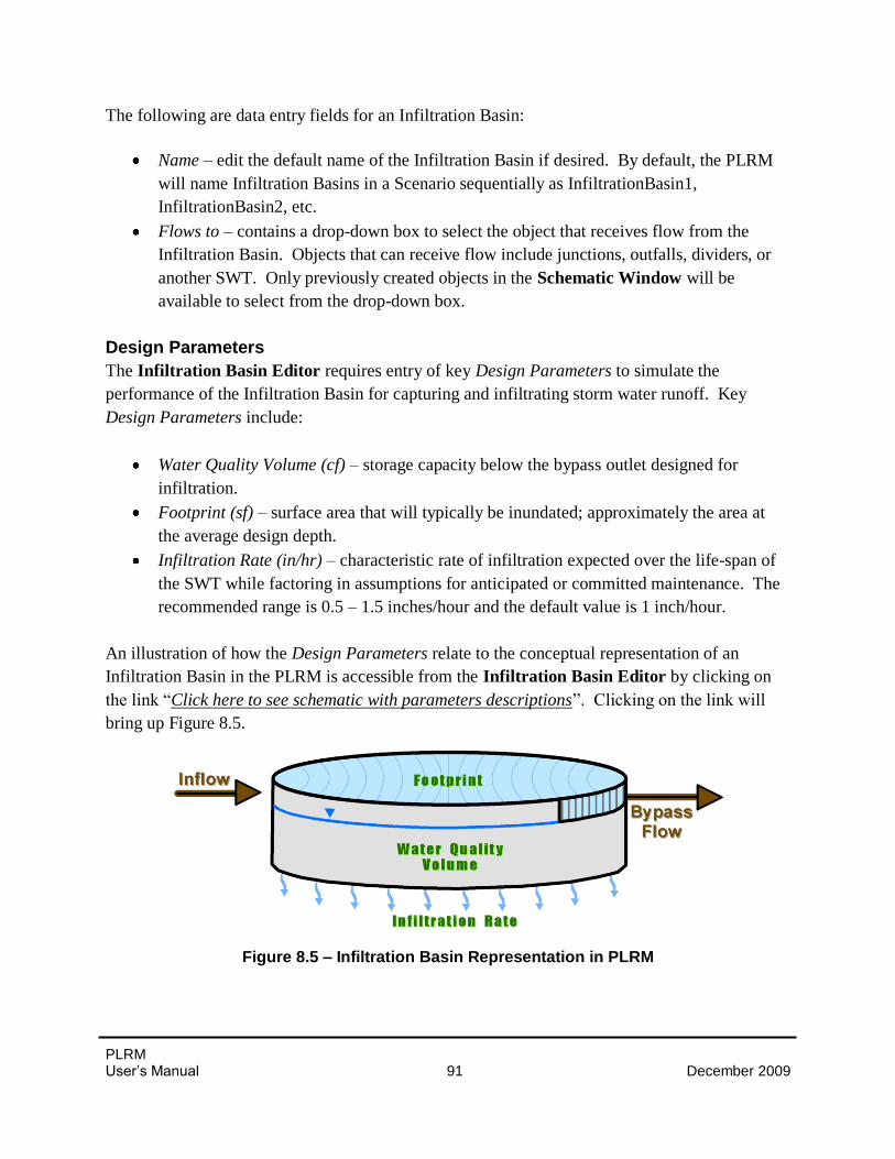
PLRM User’s Manual 91 December 2009
The following are data entry fields for an Infiltration Basin:
Name – edit the default name of the Infiltration Basin if desired. By default, the PLRM
will name Infiltration Basins in a Scenario sequentially as InfiltrationBasin1,
InfiltrationBasin2, etc.
Flows to – contains a drop-down box to select the object that receives flow from the
Infiltration Basin. Objects that can receive flow include junctions, outfalls, dividers, or
another SWT. Only previously created objects in the Schematic Window will be
available to select from the drop-down box.
Design Parameters
The Infiltration Basin Editor requires entry of key Design Parameters to simulate the
performance of the Infiltration Basin for capturing and infiltrating storm water runoff. Key
Design Parameters include:
Water Quality Volume (cf) – storage capacity below the bypass outlet designed for
infiltration.
Footprint (sf) – surface area that will typically be inundated; approximately the area at
the average design depth.
Infiltration Rate (in/hr) – characteristic rate of infiltration expected over the life-span of
the SWT while factoring in assumptions for anticipated or committed maintenance. The
recommended range is 0.5 – 1.5 inches/hour and the default value is 1 inch/hour.
An illustration of how the Design Parameters relate to the conceptual representation of an
Infiltration Basin in the PLRM is accessible from the Infiltration Basin Editor by clicking on
the link “Click here to see schematic with parameters descriptions”. Clicking on the link will
bring up Figure 8.5.
Figure 8.5 – Infiltration Basin Representation in PLRM
PLRM User’s Manual 92 December 2009
Pollutant load reductions from Infiltration Basins in the PLRM are a function of volume losses
via infiltration of the Water Quality Volume. The volume of infiltrated storm water as well as an
estimate of pollutant load removed from surface water by infiltration is tracked by the PLRM.
Storm water that bypasses the Infiltration Basin through the bypass outlet when the Water
Quality Volume is exceeded is considered Bypass Flow. The quality of Bypass Flow is equal to
the influent concentration of the storm water entering the Infiltration Basin. Note that Infiltration
Basins do not include a treatment outlet. Hence, there are no CECs for Infiltration Basins and
treatment is assumed to only occur via volume reductions from infiltration.
Customized Infiltration Rate
The Infiltration Basin Editor provides a function that allows the user to customize the
Infiltration Rate as a function of Water Quality Volume to account for head dependent infiltration
rates or variable stage-area relationships. This function can be accessed by clicking on the
Custom Volume-Discharge Curve button from the Infiltration Basin Editor (Figure 8.4).
Clicking on the button will activate the Volume-Discharge Curve Editor (Figure 8.6). The
column “Volume (cf)” divides the user-defined Water Quality Volume entered in the Infiltration
Basin Editor into ten increments. For each increment, the user can set the Infiltration Rate
(in/hr) of the Infiltration Basin. The following functions can be performed from the Volume-
Discharge Curve Editor:
Save and Close – informs the user of calculated average Infiltration Rate based on their
values entered for each volume increment. Information entered in the form is saved and
the PLRM returns to the Infiltration Basin Editor.
Auto Calculate – restores the values of Infiltration Rate based on design parameters
entered from the Infiltration Basin Editor. The default is a constant infiltration rate for
all storage volume increments greater than zero.
Cancel – disregards changes to the form and returns to the Infiltration Basin Editor.
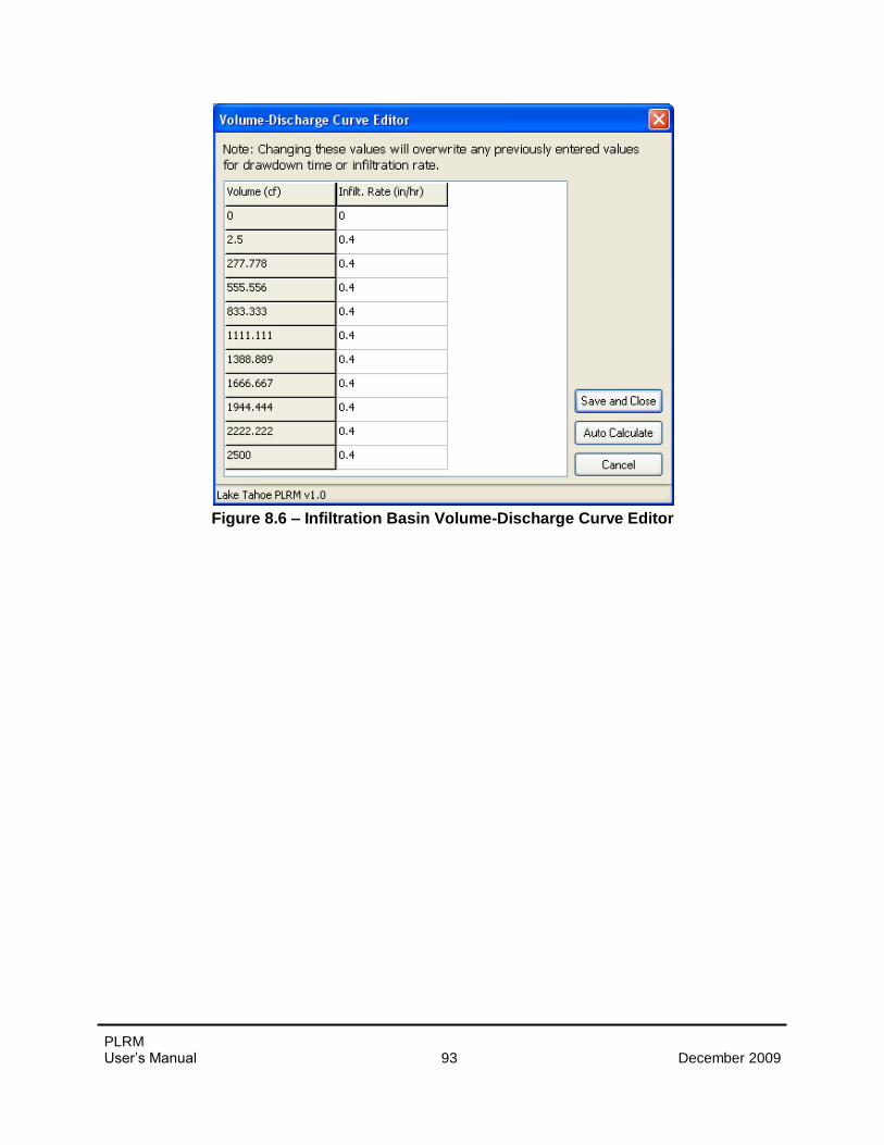
PLRM User’s Manual 93 December 2009
Figure 8.6 – Infiltration Basin Volume-Discharge Curve Editor
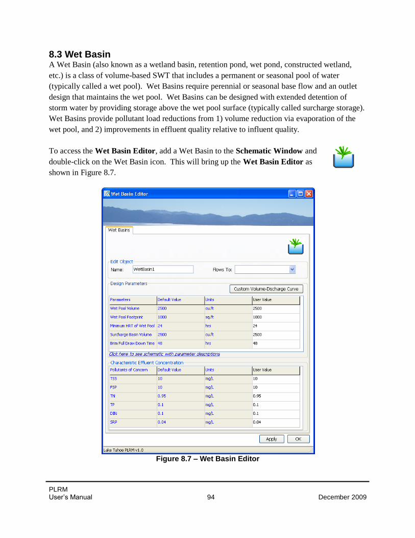
PLRM User’s Manual 94 December 2009
8.3 Wet Basin A Wet Basin (also known as a wetland basin, retention pond, wet pond, constructed wetland,
etc.) is a class of volume-based SWT that includes a permanent or seasonal pool of water
(typically called a wet pool). Wet Basins require perennial or seasonal base flow and an outlet
design that maintains the wet pool. Wet Basins can be designed with extended detention of
storm water by providing storage above the wet pool surface (typically called surcharge storage).
Wet Basins provide pollutant load reductions from 1) volume reduction via evaporation of the
wet pool, and 2) improvements in effluent quality relative to influent quality.
To access the Wet Basin Editor, add a Wet Basin to the Schematic Window and
double-click on the Wet Basin icon. This will bring up the Wet Basin Editor as
shown in Figure 8.7.
Figure 8.7 – Wet Basin Editor
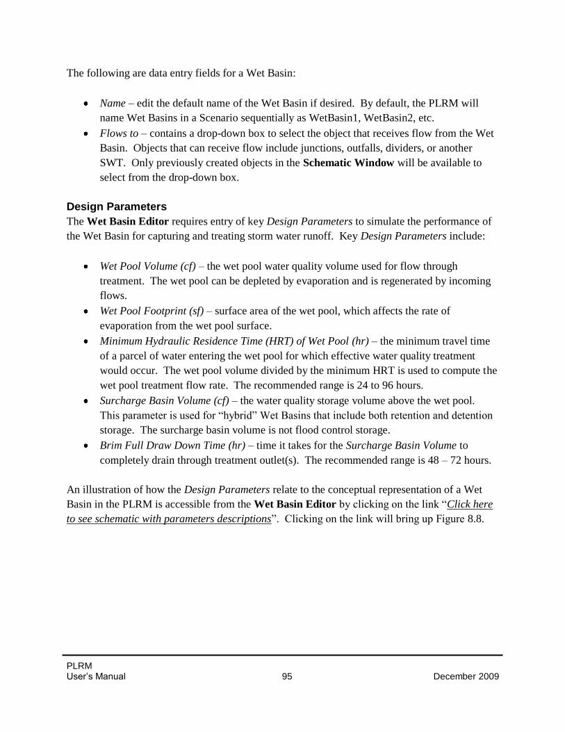
PLRM User’s Manual 95 December 2009
The following are data entry fields for a Wet Basin:
Name – edit the default name of the Wet Basin if desired. By default, the PLRM will
name Wet Basins in a Scenario sequentially as WetBasin1, WetBasin2, etc.
Flows to – contains a drop-down box to select the object that receives flow from the Wet
Basin. Objects that can receive flow include junctions, outfalls, dividers, or another
SWT. Only previously created objects in the Schematic Window will be available to
select from the drop-down box.
Design Parameters
The Wet Basin Editor requires entry of key Design Parameters to simulate the performance of
the Wet Basin for capturing and treating storm water runoff. Key Design Parameters include:
Wet Pool Volume (cf) – the wet pool water quality volume used for flow through
treatment. The wet pool can be depleted by evaporation and is regenerated by incoming
flows.
Wet Pool Footprint (sf) – surface area of the wet pool, which affects the rate of
evaporation from the wet pool surface.
Minimum Hydraulic Residence Time (HRT) of Wet Pool (hr) – the minimum travel time
of a parcel of water entering the wet pool for which effective water quality treatment
would occur. The wet pool volume divided by the minimum HRT is used to compute the
wet pool treatment flow rate. The recommended range is 24 to 96 hours.
Surcharge Basin Volume (cf) – the water quality storage volume above the wet pool.
This parameter is used for “hybrid” Wet Basins that include both retention and detention
storage. The surcharge basin volume is not flood control storage.
Brim Full Draw Down Time (hr) – time it takes for the Surcharge Basin Volume to
completely drain through treatment outlet(s). The recommended range is 48 – 72 hours.
An illustration of how the Design Parameters relate to the conceptual representation of a Wet
Basin in the PLRM is accessible from the Wet Basin Editor by clicking on the link “Click here
to see schematic with parameters descriptions”. Clicking on the link will bring up Figure 8.8.
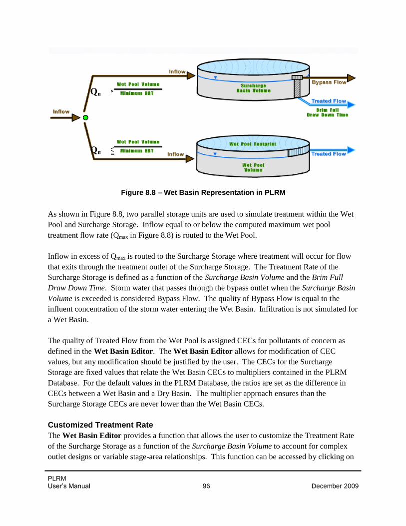
PLRM User’s Manual 96 December 2009
Figure 8.8 – Wet Basin Representation in PLRM
As shown in Figure 8.8, two parallel storage units are used to simulate treatment within the Wet
Pool and Surcharge Storage. Inflow equal to or below the computed maximum wet pool
treatment flow rate (Qmax in Figure 8.8) is routed to the Wet Pool.
Inflow in excess of Qmax is routed to the Surcharge Storage where treatment will occur for flow
that exits through the treatment outlet of the Surcharge Storage. The Treatment Rate of the
Surcharge Storage is defined as a function of the Surcharge Basin Volume and the Brim Full
Draw Down Time. Storm water that passes through the bypass outlet when the Surcharge Basin
Volume is exceeded is considered Bypass Flow. The quality of Bypass Flow is equal to the
influent concentration of the storm water entering the Wet Basin. Infiltration is not simulated for
a Wet Basin.
The quality of Treated Flow from the Wet Pool is assigned CECs for pollutants of concern as
defined in the Wet Basin Editor. The Wet Basin Editor allows for modification of CEC
values, but any modification should be justified by the user. The CECs for the Surcharge
Storage are fixed values that relate the Wet Basin CECs to multipliers contained in the PLRM
Database. For the default values in the PLRM Database, the ratios are set as the difference in
CECs between a Wet Basin and a Dry Basin. The multiplier approach ensures than the
Surcharge Storage CECs are never lower than the Wet Basin CECs.
Customized Treatment Rate
The Wet Basin Editor provides a function that allows the user to customize the Treatment Rate
of the Surcharge Storage as a function of the Surcharge Basin Volume to account for complex
outlet designs or variable stage-area relationships. This function can be accessed by clicking on
Qmax<
Qmax>
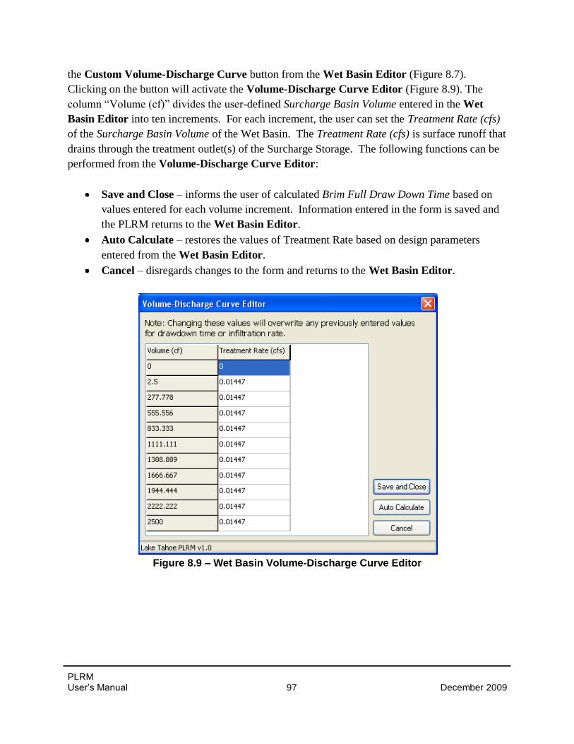
PLRM User’s Manual 97 December 2009
the Custom Volume-Discharge Curve button from the Wet Basin Editor (Figure 8.7).
Clicking on the button will activate the Volume-Discharge Curve Editor (Figure 8.9). The
column “Volume (cf)” divides the user-defined Surcharge Basin Volume entered in the Wet
Basin Editor into ten increments. For each increment, the user can set the Treatment Rate (cfs)
of the Surcharge Basin Volume of the Wet Basin. The Treatment Rate (cfs) is surface runoff that
drains through the treatment outlet(s) of the Surcharge Storage. The following functions can be
performed from the Volume-Discharge Curve Editor:
Save and Close – informs the user of calculated Brim Full Draw Down Time based on
values entered for each volume increment. Information entered in the form is saved and
the PLRM returns to the Wet Basin Editor.
Auto Calculate – restores the values of Treatment Rate based on design parameters
entered from the Wet Basin Editor.
Cancel – disregards changes to the form and returns to the Wet Basin Editor.
Figure 8.9 – Wet Basin Volume-Discharge Curve Editor
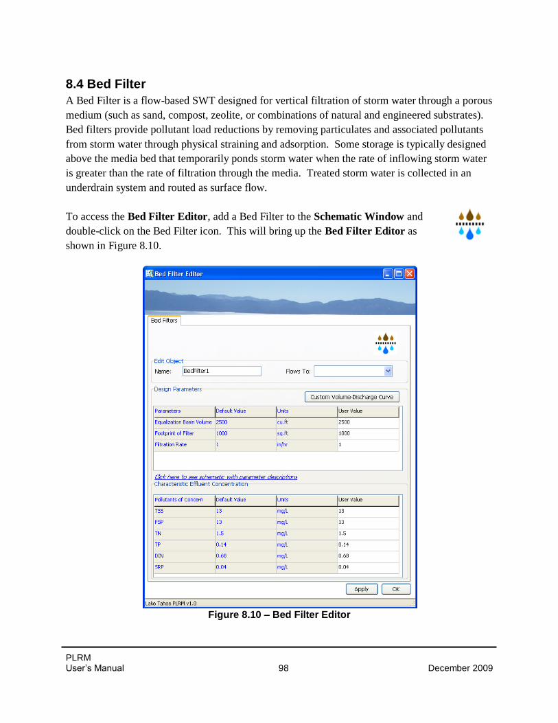
PLRM User’s Manual 98 December 2009
8.4 Bed Filter
A Bed Filter is a flow-based SWT designed for vertical filtration of storm water through a porous
medium (such as sand, compost, zeolite, or combinations of natural and engineered substrates).
Bed filters provide pollutant load reductions by removing particulates and associated pollutants
from storm water through physical straining and adsorption. Some storage is typically designed
above the media bed that temporarily ponds storm water when the rate of inflowing storm water
is greater than the rate of filtration through the media. Treated storm water is collected in an
underdrain system and routed as surface flow.
To access the Bed Filter Editor, add a Bed Filter to the Schematic Window and
double-click on the Bed Filter icon. This will bring up the Bed Filter Editor as
shown in Figure 8.10.
Figure 8.10 – Bed Filter Editor
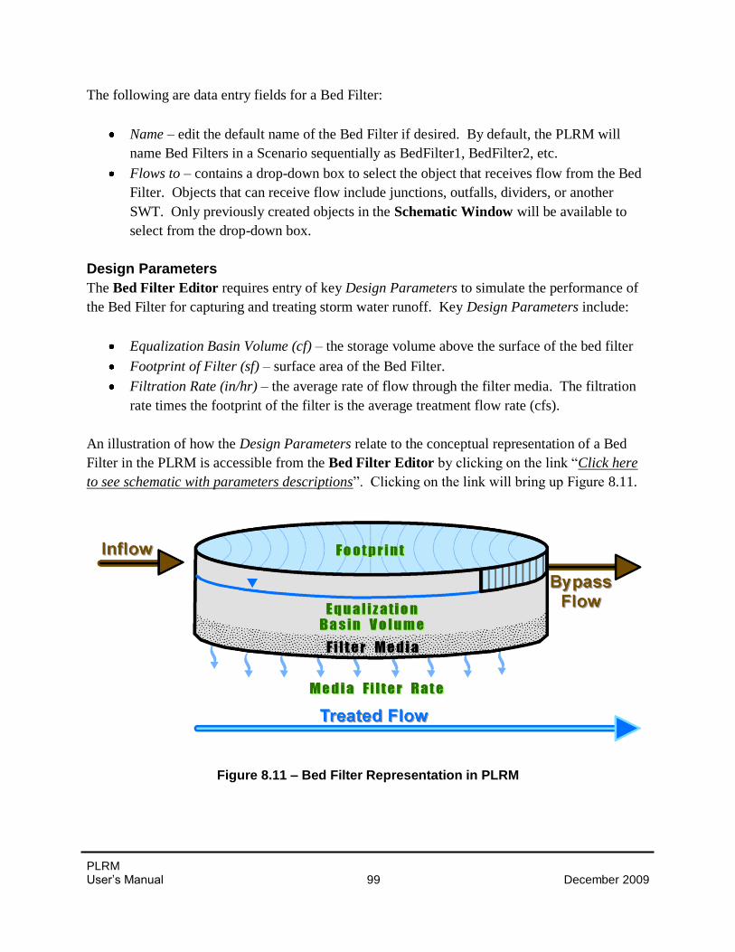
PLRM User’s Manual 99 December 2009
The following are data entry fields for a Bed Filter:
Name – edit the default name of the Bed Filter if desired. By default, the PLRM will
name Bed Filters in a Scenario sequentially as BedFilter1, BedFilter2, etc.
Flows to – contains a drop-down box to select the object that receives flow from the Bed
Filter. Objects that can receive flow include junctions, outfalls, dividers, or another
SWT. Only previously created objects in the Schematic Window will be available to
select from the drop-down box.
Design Parameters
The Bed Filter Editor requires entry of key Design Parameters to simulate the performance of
the Bed Filter for capturing and treating storm water runoff. Key Design Parameters include:
Equalization Basin Volume (cf) – the storage volume above the surface of the bed filter
Footprint of Filter (sf) – surface area of the Bed Filter.
Filtration Rate (in/hr) – the average rate of flow through the filter media. The filtration
rate times the footprint of the filter is the average treatment flow rate (cfs).
An illustration of how the Design Parameters relate to the conceptual representation of a Bed
Filter in the PLRM is accessible from the Bed Filter Editor by clicking on the link “Click here
to see schematic with parameters descriptions”. Clicking on the link will bring up Figure 8.11.
Figure 8.11 – Bed Filter Representation in PLRM
PLRM User’s Manual 100 December 2009
As shown in Figure 8.11, storm water that passes through the filter media is considered Treated
Flow. The quality of Treated Flow from the Bed Filter is assigned CECs for pollutants of
concern as defined in the Bed Filter Editor. If the incoming flow rate exceeds the treatment
flow rate, the Equalization Basin Volume above the filter bed will begin to fill. Storm water that
passes through the bypass outlet when the Equalization Basin Volume is exceeded is considered
Bypass Flow. The quality of Bypass Flow is equal to the influent concentration of the storm
water entering the Bed Filter. The Bed Filter Editor allows for modification of CEC values, but
any modification should be justified by the user.
Customized Filtration Rate
The Bed Filter Editor provides a function that allows the user to customize Filtration Rate as a
function of the Equalization Basin Volume to account for head dependent filtration rates or
variable stage-area relationships. This function can be accessed by clicking on the Custom
Volume-Discharge Curve button from the Bed Filter Editor (Figure 8.10). Clicking on the
button will activate the Volume-Discharge Curve Editor (Figure 8.12). The column “Volume
(cf)” divides the user-defined Equalization Basin Volume entered in the Bed Filter Editor into
ten increments. For each increment, the user can set the Filtration Rate (inch/hr) of the Bed
Filter. The following functions can be performed from the Volume-Discharge Curve Editor:
Save and Close – informs the user of calculated average Filtration Rate based on values
entered for each volume increment. Information entered in the form is saved and the
PLRM returns to the Bed Filter Editor.
Auto Calculate – restores the values of Filtration Rate based on the design parameters
entered from the Bed Filter Editor. The default is a constant filtration rate for all storage
volume increments greater than zero.
Cancel – disregards changes to the form and returns to the Bed Filter Editor.
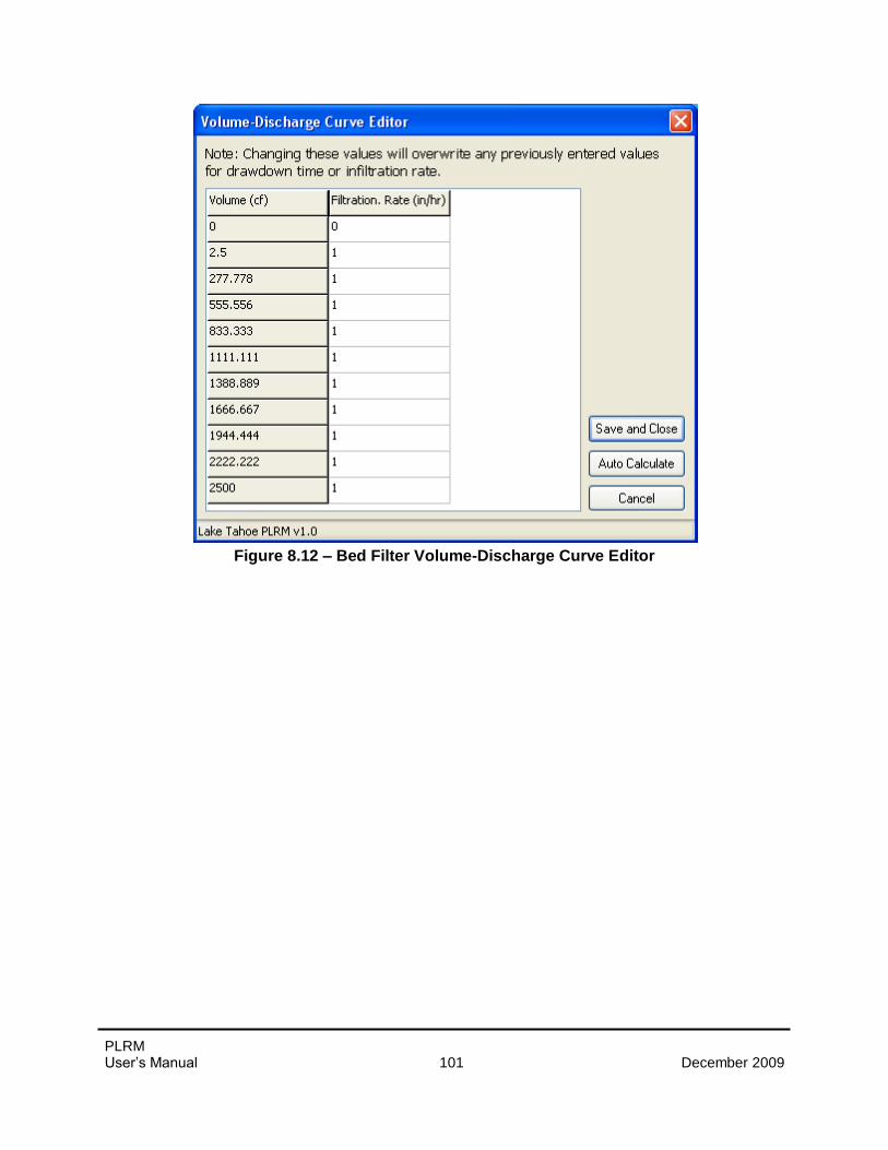
PLRM User’s Manual 101 December 2009
Figure 8.12 – Bed Filter Volume-Discharge Curve Editor
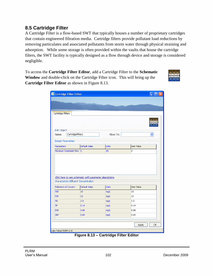
PLRM User’s Manual 102 December 2009
8.5 Cartridge Filter A Cartridge Filter is a flow-based SWT that typically houses a number of proprietary cartridges
that contain engineered filtration media. Cartridge filters provide pollutant load reductions by
removing particulates and associated pollutants from storm water through physical straining and
adsorption. While some storage is often provided within the vaults that house the cartridge
filters, the SWT facility is typically designed as a flow through device and storage is considered
negligible.
To access the Cartridge Filter Editor, add a Cartridge Filter to the Schematic
Window and double-click on the Cartridge Filter icon. This will bring up the
Cartridge Filter Editor as shown in Figure 8.13.
Figure 8.13 – Cartridge Filter Editor
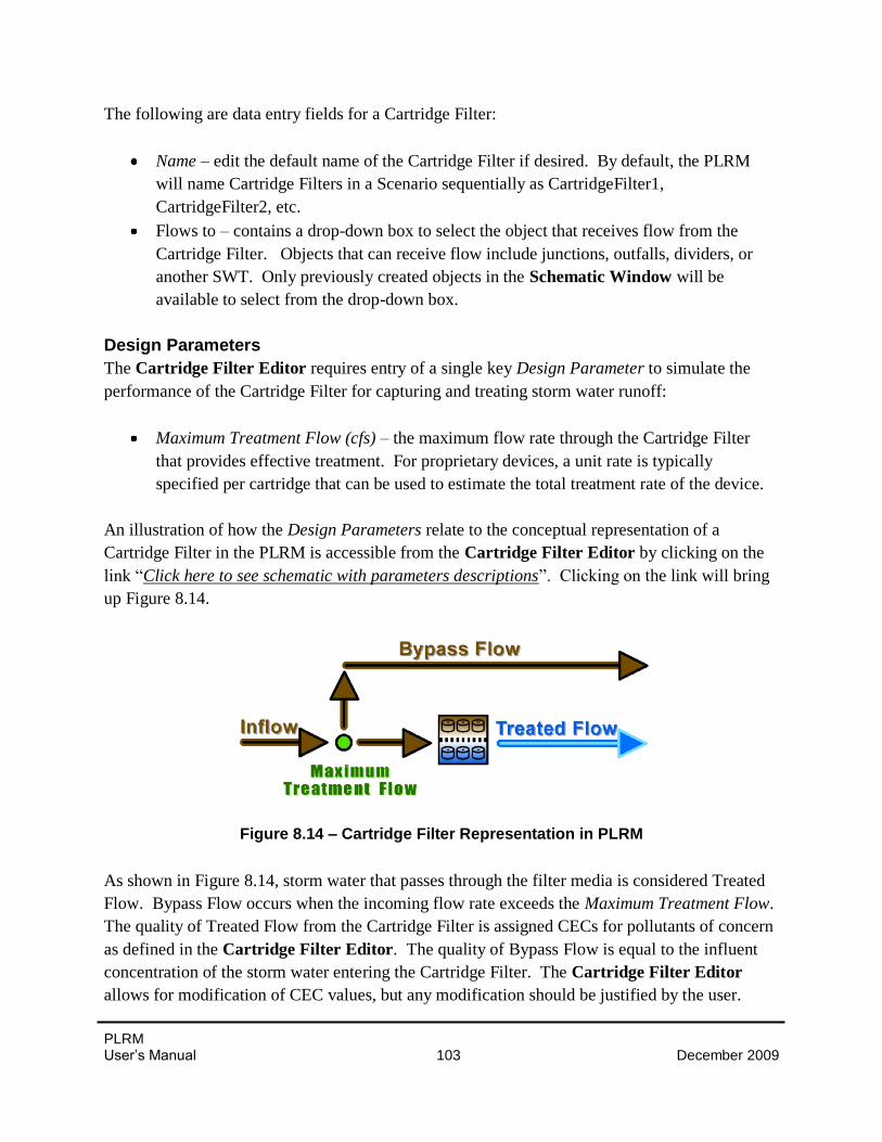
PLRM User’s Manual 103 December 2009
The following are data entry fields for a Cartridge Filter:
Name – edit the default name of the Cartridge Filter if desired. By default, the PLRM
will name Cartridge Filters in a Scenario sequentially as CartridgeFilter1,
CartridgeFilter2, etc.
Flows to – contains a drop-down box to select the object that receives flow from the
Cartridge Filter. Objects that can receive flow include junctions, outfalls, dividers, or
another SWT. Only previously created objects in the Schematic Window will be
available to select from the drop-down box.
Design Parameters
The Cartridge Filter Editor requires entry of a single key Design Parameter to simulate the
performance of the Cartridge Filter for capturing and treating storm water runoff:
Maximum Treatment Flow (cfs) – the maximum flow rate through the Cartridge Filter
that provides effective treatment. For proprietary devices, a unit rate is typically
specified per cartridge that can be used to estimate the total treatment rate of the device.
An illustration of how the Design Parameters relate to the conceptual representation of a
Cartridge Filter in the PLRM is accessible from the Cartridge Filter Editor by clicking on the
link “Click here to see schematic with parameters descriptions”. Clicking on the link will bring
up Figure 8.14.
Figure 8.14 – Cartridge Filter Representation in PLRM
As shown in Figure 8.14, storm water that passes through the filter media is considered Treated
Flow. Bypass Flow occurs when the incoming flow rate exceeds the Maximum Treatment Flow.
The quality of Treated Flow from the Cartridge Filter is assigned CECs for pollutants of concern
as defined in the Cartridge Filter Editor. The quality of Bypass Flow is equal to the influent
concentration of the storm water entering the Cartridge Filter. The Cartridge Filter Editor
allows for modification of CEC values, but any modification should be justified by the user.
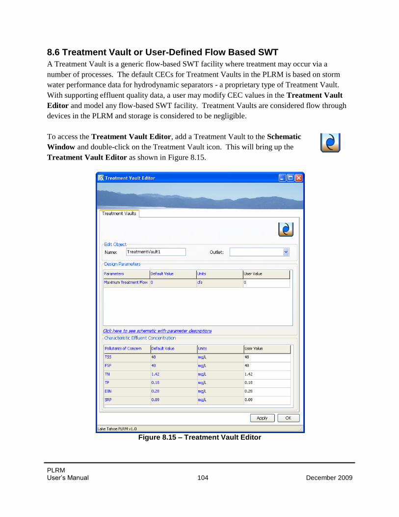
PLRM User’s Manual 104 December 2009
8.6 Treatment Vault or User-Defined Flow Based SWT
A Treatment Vault is a generic flow-based SWT facility where treatment may occur via a
number of processes. The default CECs for Treatment Vaults in the PLRM is based on storm
water performance data for hydrodynamic separators - a proprietary type of Treatment Vault.
With supporting effluent quality data, a user may modify CEC values in the Treatment Vault
Editor and model any flow-based SWT facility. Treatment Vaults are considered flow through
devices in the PLRM and storage is considered to be negligible.
To access the Treatment Vault Editor, add a Treatment Vault to the Schematic
Window and double-click on the Treatment Vault icon. This will bring up the
Treatment Vault Editor as shown in Figure 8.15.
Figure 8.15 – Treatment Vault Editor
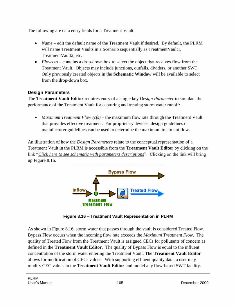
PLRM User’s Manual 105 December 2009
The following are data entry fields for a Treatment Vault:
Name – edit the default name of the Treatment Vault if desired. By default, the PLRM
will name Treatment Vaults in a Scenario sequentially as TreatmentVault1,
TreatmentVault2, etc.
Flows to – contains a drop-down box to select the object that receives flow from the
Treatment Vault. Objects may include junctions, outfalls, dividers, or another SWT.
Only previously created objects in the Schematic Window will be available to select
from the drop-down box.
Design Parameters
The Treatment Vault Editor requires entry of a single key Design Parameter to simulate the
performance of the Treatment Vault for capturing and treating storm water runoff:
Maximum Treatment Flow (cfs) – the maximum flow rate through the Treatment Vault
that provides effective treatment. For proprietary devices, design guidelines or
manufacturer guidelines can be used to determine the maximum treatment flow.
An illustration of how the Design Parameters relate to the conceptual representation of a
Treatment Vault in the PLRM is accessible from the Treatment Vault Editor by clicking on the
link “Click here to see schematic with parameters descriptions”. Clicking on the link will bring
up Figure 8.16.
Figure 8.16 – Treatment Vault Representation in PLRM
As shown in Figure 8.16, storm water that passes through the vault is considered Treated Flow.
Bypass Flow occurs when the incoming flow rate exceeds the Maximum Treatment Flow. The
quality of Treated Flow from the Treatment Vault is assigned CECs for pollutants of concern as
defined in the Treatment Vault Editor. The quality of Bypass Flow is equal to the influent
concentration of the storm water entering the Treatment Vault. The Treatment Vault Editor
allows for modification of CECs values. With supporting effluent quality data, a user may
modify CEC values in the Treatment Vault Editor and model any flow-based SWT facility.
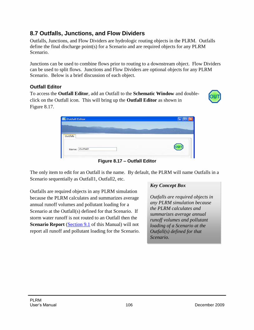
PLRM User’s Manual 106 December 2009
8.7 Outfalls, Junctions, and Flow Dividers
Outfalls, Junctions, and Flow Dividers are hydrologic routing objects in the PLRM. Outfalls
define the final discharge point(s) for a Scenario and are required objects for any PLRM
Scenario.
Junctions can be used to combine flows prior to routing to a downstream object. Flow Dividers
can be used to split flows. Junctions and Flow Dividers are optional objects for any PLRM
Scenario. Below is a brief discussion of each object.
Outfall Editor
To access the Outfall Editor, add an Outfall to the Schematic Window and double-
click on the Outfall icon. This will bring up the Outfall Editor as shown in
Figure 8.17.
Figure 8.17 – Outfall Editor
The only item to edit for an Outfall is the name. By default, the PLRM will name Outfalls in a
Scenario sequentially as Outfall1, Outfall2, etc.
Outfalls are required objects in any PLRM simulation
because the PLRM calculates and summarizes average
annual runoff volumes and pollutant loading for a
Scenario at the Outfall(s) defined for that Scenario. If
storm water runoff is not routed to an Outfall then the
Scenario Report (Section 9.1 of this Manual) will not
report all runoff and pollutant loading for the Scenario.
Key Concept Box
Outfalls are required objects in
any PLRM simulation because
the PLRM calculates and
summarizes average annual
runoff volumes and pollutant
loading of a Scenario at the
Outfall(s) defined for that
Scenario.
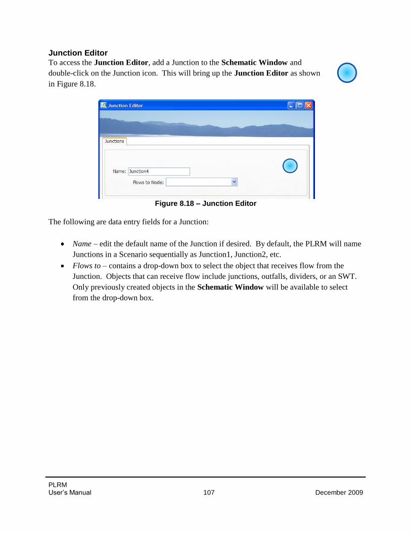
PLRM User’s Manual 107 December 2009
Junction Editor To access the Junction Editor, add a Junction to the Schematic Window and
double-click on the Junction icon. This will bring up the Junction Editor as shown
in Figure 8.18.
Figure 8.18 – Junction Editor
The following are data entry fields for a Junction:
Name – edit the default name of the Junction if desired. By default, the PLRM will name
Junctions in a Scenario sequentially as Junction1, Junction2, etc.
Flows to – contains a drop-down box to select the object that receives flow from the
Junction. Objects that can receive flow include junctions, outfalls, dividers, or an SWT.
Only previously created objects in the Schematic Window will be available to select
from the drop-down box.
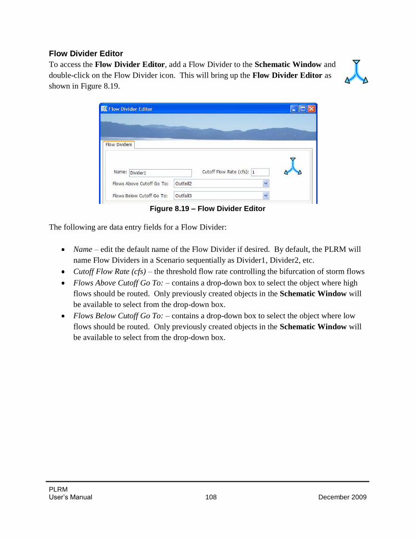
PLRM User’s Manual 108 December 2009
Flow Divider Editor
To access the Flow Divider Editor, add a Flow Divider to the Schematic Window and
double-click on the Flow Divider icon. This will bring up the Flow Divider Editor as
shown in Figure 8.19.
Figure 8.19 – Flow Divider Editor
The following are data entry fields for a Flow Divider:
Name – edit the default name of the Flow Divider if desired. By default, the PLRM will
name Flow Dividers in a Scenario sequentially as Divider1, Divider2, etc.
Cutoff Flow Rate (cfs) – the threshold flow rate controlling the bifurcation of storm flows
Flows Above Cutoff Go To: – contains a drop-down box to select the object where high
flows should be routed. Only previously created objects in the Schematic Window will
be available to select from the drop-down box.
Flows Below Cutoff Go To: – contains a drop-down box to select the object where low
flows should be routed. Only previously created objects in the Schematic Window will
be available to select from the drop-down box.
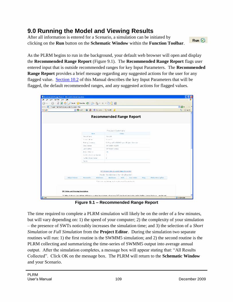
PLRM User’s Manual 109 December 2009
9.0 Running the Model and Viewing Results After all information is entered for a Scenario, a simulation can be initiated by
clicking on the Run button on the Schematic Window within the Function Toolbar.
As the PLRM begins to run in the background, your default web browser will open and display
the Recommended Range Report (Figure 9.1). The Recommended Range Report flags user
entered input that is outside recommended ranges for key Input Parameters. The Recommended
Range Report provides a brief message regarding any suggested actions for the user for any
flagged value. Section 10.2 of this Manual describes the key Input Parameters that will be
flagged, the default recommended ranges, and any suggested actions for flagged values.
Figure 9.1 – Recommended Range Report
The time required to complete a PLRM simulation will likely be on the order of a few minutes,
but will vary depending on: 1) the speed of your computer; 2) the complexity of your simulation
– the presence of SWTs noticeably increases the simulation time; and 3) the selection of a Short
Simulation or Full Simulation from the Project Editor. During the simulation two separate
routines will run: 1) the first routine is the SWMM5 simulation; and 2) the second routine is the
PLRM collecting and summarizing the time-series of SWMM5 output into average annual
output. After the simulation completes, a message box will appear stating that: “All Results
Collected”. Click OK on the message box. The PLRM will return to the Schematic Window
and your Scenario.
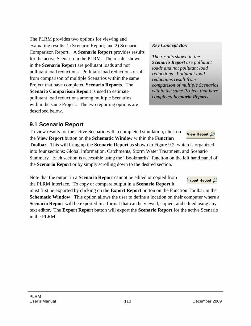
PLRM User’s Manual 110 December 2009
The PLRM provides two options for viewing and
evaluating results: 1) Scenario Report; and 2) Scenario
Comparison Report. A Scenario Report provides results
for the active Scenario in the PLRM. The results shown
in the Scenario Report are pollutant loads and not
pollutant load reductions. Pollutant load reductions result
from comparison of multiple Scenarios within the same
Project that have completed Scenario Reports. The
Scenario Comparison Report is used to estimate
pollutant load reductions among multiple Scenarios
within the same Project. The two reporting options are
described below.
9.1 Scenario Report
To view results for the active Scenario with a completed simulation, click on
the View Report button on the Schematic Window within the Function
Toolbar. This will bring up the Scenario Report as shown in Figure 9.2, which is organized
into four sections: Global Information, Catchments, Storm Water Treatment, and Scenario
Summary. Each section is accessible using the “Bookmarks” function on the left hand panel of
the Scenario Report or by simply scrolling down to the desired section.
Note that the output in a Scenario Report cannot be edited or copied from
the PLRM Interface. To copy or compare output in a Scenario Report it
must first be exported by clicking on the Export Report button on the Function Toolbar in the
Schematic Window. This option allows the user to define a location on their computer where a
Scenario Report will be exported in a format that can be viewed, copied, and edited using any
text editor. The Export Report button will export the Scenario Report for the active Scenario
in the PLRM.
Key Concept Box
The results shown in the
Scenario Report are pollutant
loads and not pollutant load
reductions. Pollutant load
reductions result from
comparison of multiple Scenarios
within the same Project that have
completed Scenario Reports.
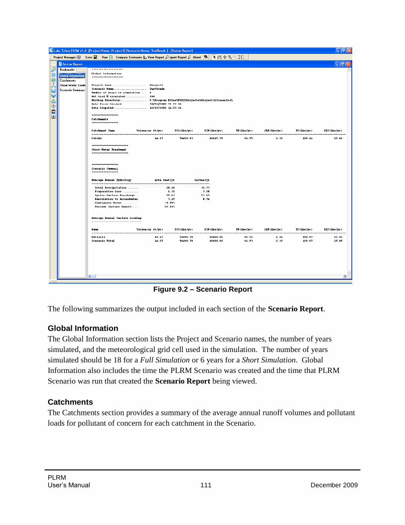
PLRM User’s Manual 111 December 2009
Figure 9.2 – Scenario Report
The following summarizes the output included in each section of the Scenario Report.
Global Information
The Global Information section lists the Project and Scenario names, the number of years
simulated, and the meteorological grid cell used in the simulation. The number of years
simulated should be 18 for a Full Simulation or 6 years for a Short Simulation. Global
Information also includes the time the PLRM Scenario was created and the time that PLRM
Scenario was run that created the Scenario Report being viewed.
Catchments
The Catchments section provides a summary of the average annual runoff volumes and pollutant
loads for pollutant of concern for each catchment in the Scenario.
PLRM User’s Manual 112 December 2009
Storm Water Treatment
The Storm Water Treatment section summarizes for each SWT facility in the Scenario the
following:
Total Influent – average annual runoff volume and pollutant load to the SWT facility
Bypass Stream – average annual runoff volume and pollutant load not captured by the
SWT facility (i.e. runoff and pollutant load bypassing the SWT facility)
Treatment Stream – average annual runoff volume captured and treated by the SWT
facility; average annual pollutant load remaining after treatment by the SWT facility
Total Effluent – combined bypass stream and treated stream; average annual runoff and
pollutant load downstream of the SWT facility
Volume/Load Removed – average annual runoff volume and pollutant load removed by
the SWT facility
% Change (Removed/Influent) – relative percent of average annual runoff volume and
pollutant load removed. Note that the subtraction or addition of PSCs and HSCs to the
catchment(s) draining to an SWT will influence the load removed by the SWT.
% Capture (1- Bypass/Influent) – average annual hydraulic capture of the SWT or the
percent of the influent volume captured and treated and/or infiltrated by the SWT. The
percent capture is an important performance metric that provides an indication of the
effectiveness of the hydraulic design of the SWT relative to inflowing storm water
characteristics. For example, a target percent capture of 80% - 90% is common in
practice because this range is typically the “point of diminishing returns” where small
incremental increases in the percent capture require a much larger facility.
Hydraulic capture increases for short drain times or high infiltration/filtration rates. Short
drain times decrease the time it takes for an SWT to recover its storage capacity. For
actual SWT facilities, short drain times may not provide the hydraulic residence
necessary to achieve the Characteristic Effluent Concentrations (CECs) assumed in the
PLRM. For this reason, recommended limits for several input parameters that affect
hydraulic capture are provided in Section 10.2. For example, the minimum
recommended brim full drawdown time for a Dry Basin is 48 hours.

PLRM User’s Manual 113 December 2009
Scenario Summary The Scenario Summary section summarizes average annual hydrology and surface loading.
The hydrology summary includes average annual precipitation, evaporation losses, system
surface discharge, and percolation to groundwater. The summary also calculates a water balance
continuity error and the percent of rainfall that generates surface runoff.
The surface loading summary provides average annual runoff volumes and pollutant loading for
each outfall in the Scenario, as well as Scenario Total. The Scenario Total is simply the sum of
the runoff volumes and pollutant loads for all outfalls in the Scenario. The Scenario Total is
used by the Scenario Comparison Report to estimate pollutant load reductions among
Scenarios.
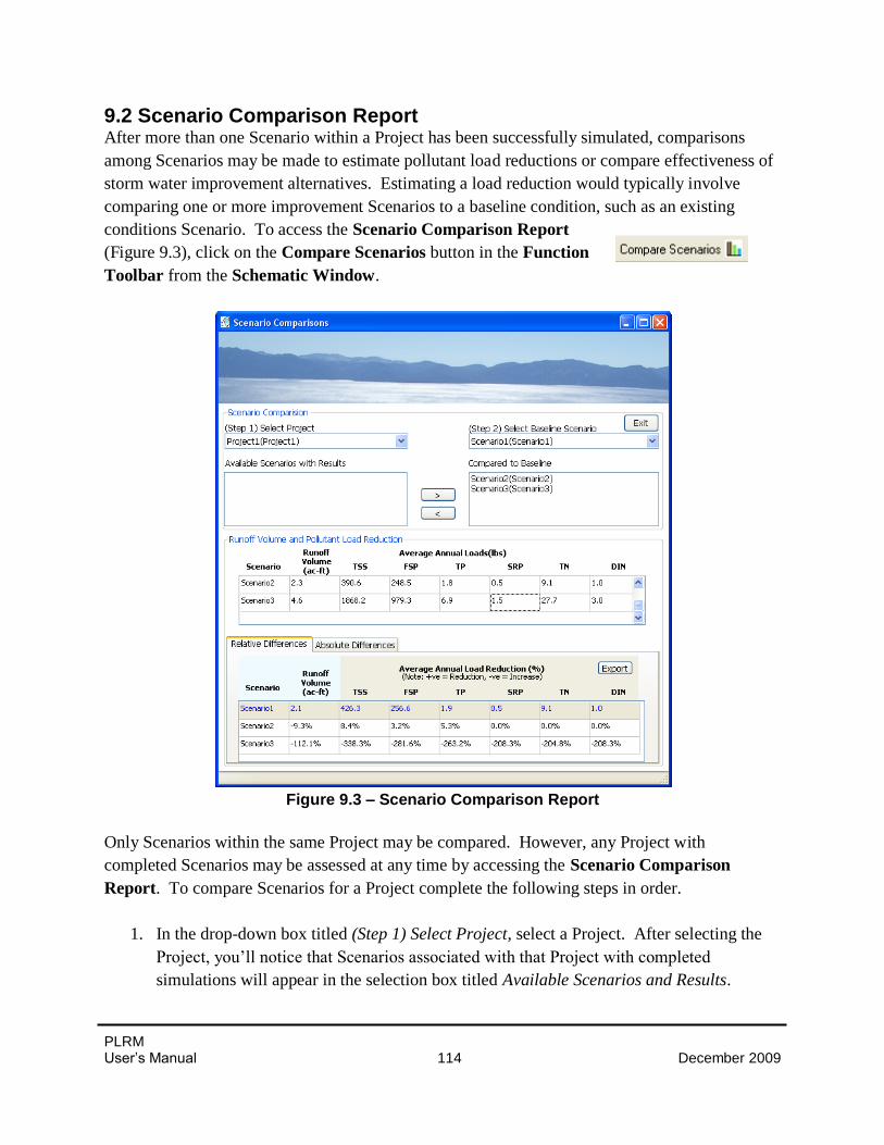
PLRM User’s Manual 114 December 2009
9.2 Scenario Comparison Report After more than one Scenario within a Project has been successfully simulated, comparisons
among Scenarios may be made to estimate pollutant load reductions or compare effectiveness of
storm water improvement alternatives. Estimating a load reduction would typically involve
comparing one or more improvement Scenarios to a baseline condition, such as an existing
conditions Scenario. To access the Scenario Comparison Report
(Figure 9.3), click on the Compare Scenarios button in the Function
Toolbar from the Schematic Window.
Figure 9.3 – Scenario Comparison Report
Only Scenarios within the same Project may be compared. However, any Project with
completed Scenarios may be assessed at any time by accessing the Scenario Comparison
Report. To compare Scenarios for a Project complete the following steps in order.
1. In the drop-down box titled (Step 1) Select Project, select a Project. After selecting the
Project, you’ll notice that Scenarios associated with that Project with completed
simulations will appear in the selection box titled Available Scenarios and Results.
PLRM User’s Manual 115 December 2009
2. In the drop-down box titled (Step 2) Select Baseline Scenario, select a Baseline Scenario
that all other Scenarios will be compared against. The Baseline Scenario is typically the
existing conditions Scenario, but it doesn’t need to be. Once selected, the runoff volume
and pollutant loads of the Baseline Scenario are summarized at the top of the two grid
boxes at bottom of the form.
3. In the selection box titled Available Scenarios and Results, select a
Scenario to compare to the Baseline Scenario and click on the right arrow.
The runoff volume and pollutant loads of the selected Scenario will be added to the first
grid box and the pollutant load reduction between the Baseline Scenario and the selected
Scenario will be summarized in the second grid box. Multiple Scenarios within a Project
may be compared simultaneously using the approach outlined in this step.
4. Pollutant load reductions and/or comparisons of the effectiveness among various storm
water improvement alternatives may be viewed as absolute or relative values by clicking
on the tabs at the top of the second grid box.
5. The Scenario Comparison Report may be exported to a comma delimited text file by
clicking the Export button.
The Scenario Comparison Report compares and
estimates differences in total pollutant loading among
Scenarios using the Scenario Total output at the bottom of
the Scenario Report. If the user wishes to explore more
detailed results among Scenarios, such as differences in
runoff from a specific catchment attributed to varying the
levels of HSC implementation among Scenarios, then the
Scenario Reports must be compared manually.
Scenario Reports can be compared manually by first
exporting each Scenario Report using the Export Report
option on the Schematic Window within the Function
Toolbar. This option allows the user to define a location
on their computer where a Scenario Report will be exported in a format that can be viewed,
copied, and edited using any text editor. The Export Report button will export the Scenario
Report for the active Scenario in the PLRM.
Key Concept Box
The Scenario Comparison
Report compares and estimates
differences in total pollutant
loading among Scenarios using
the Scenario Total output at the
bottom of the Scenario Report.
If the user wishes to explore more
detailed results among Scenarios,
then individual Scenario Reports
must be compared manually.
PLRM User’s Manual 116 December 2009
10.0 Parameter Guidance This section provides guidance for defining key model parameters that strongly influence PLRM
model results and that require some user judgment to determine. The structure of the PLRM was
developed to streamline input data entry by limiting the number of parameters accessible from
the PLRM Interface to those that are project area specific and are sensitive in terms of
influencing PLRM output. This structure relieves the burden on the user to develop all input
data required to execute a SWMM5 simulation. Input necessary for a PLRM simulation is
similar to some of the data typically collected for a Tahoe Basin Existing Conditions Analysis
(SWQIC, 2004). Parameters accessible from the PLRM Interface are termed Input Parameters.
Parameters that are necessary for a SWMM5 simulation, but either do not strongly influence
PLRM output (e.g., Manning’s n) or are typically not project specific (e.g., snowmelt
coefficients) are included in the PLRM Database (see Section 11). Parameters that are not
directly accessible from the PLRM Interface are termed Default Parameters.
Section 10.1 describes the most sensitive Default Parameters and the way that they influence
PLRM output. Section 10.2 describes key Input Parameters. The guidance in Section 10.2 is
limited to Input Parameters that are not easily measured (e.g., percentage of directly connected
impervious area) or may vary over time (e.g., infiltration rates). Input Parameters that are easily
measured and are relatively static values (e.g., quantity of impervious area) are assumed to be
relatively straightforward for the user, and are not discussed in this section although they may
strongly influence PLRM output.
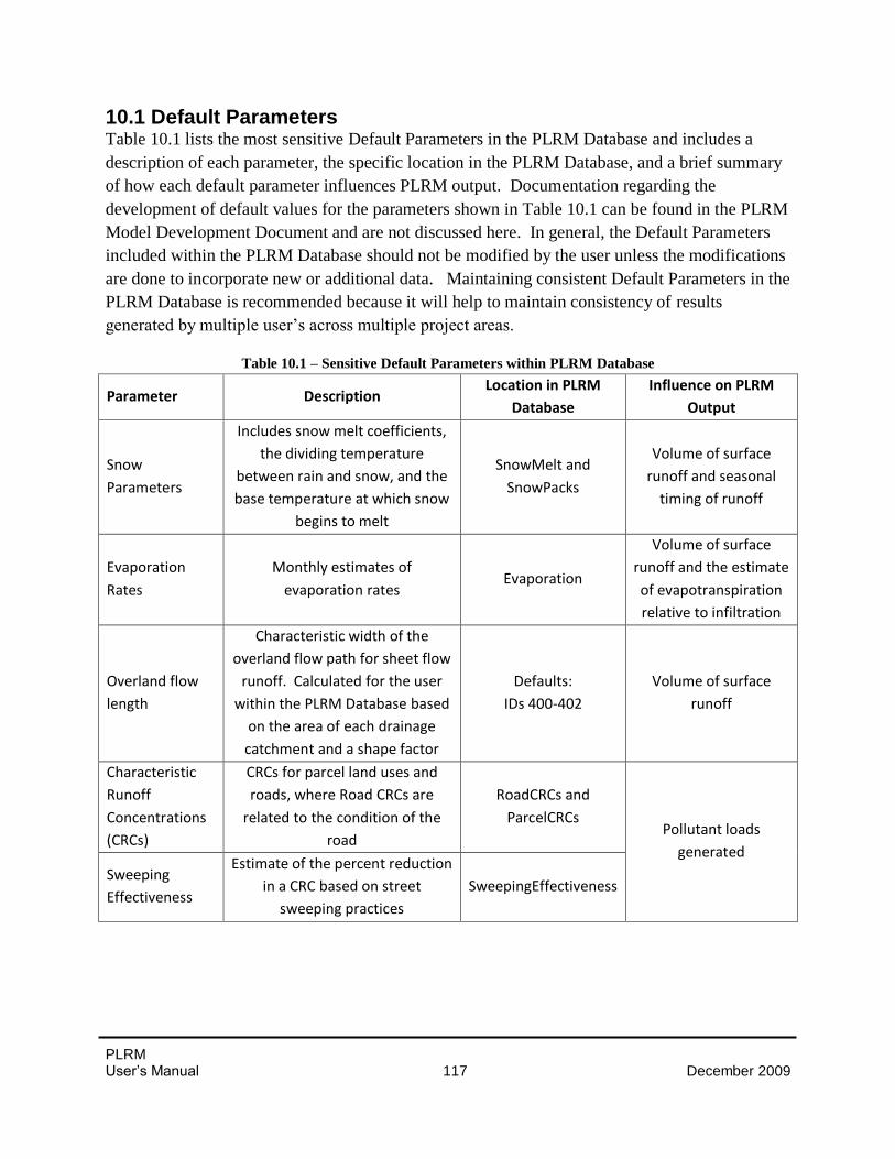
PLRM User’s Manual 117 December 2009
10.1 Default Parameters Table 10.1 lists the most sensitive Default Parameters in the PLRM Database and includes a
description of each parameter, the specific location in the PLRM Database, and a brief summary
of how each default parameter influences PLRM output. Documentation regarding the
development of default values for the parameters shown in Table 10.1 can be found in the PLRM
Model Development Document and are not discussed here. In general, the Default Parameters
included within the PLRM Database should not be modified by the user unless the modifications
are done to incorporate new or additional data. Maintaining consistent Default Parameters in the
PLRM Database is recommended because it will help to maintain consistency of results
generated by multiple user’s across multiple project areas.
Table 10.1 – Sensitive Default Parameters within PLRM Database
Parameter Description Location in PLRM
Database
Influence on PLRM
Output
Snow
Parameters
Includes snow melt coefficients,
the dividing temperature
between rain and snow, and the
base temperature at which snow
begins to melt
SnowMelt and
SnowPacks
Volume of surface
runoff and seasonal
timing of runoff
Evaporation
Rates
Monthly estimates of
evaporation rates Evaporation
Volume of surface
runoff and the estimate
of evapotranspiration
relative to infiltration
Overland flow
length
Characteristic width of the
overland flow path for sheet flow
runoff. Calculated for the user
within the PLRM Database based
on the area of each drainage
catchment and a shape factor
Defaults:
IDs 400-402
Volume of surface
runoff
Characteristic
Runoff
Concentrations
(CRCs)
CRCs for parcel land uses and
roads, where Road CRCs are
related to the condition of the
road
RoadCRCs and
ParcelCRCs Pollutant loads
generated
Sweeping
Effectiveness
Estimate of the percent reduction
in a CRC based on street
sweeping practices
SweepingEffectiveness
PLRM User’s Manual 118 December 2009
10.2 Input Parameters
Table 10.2 below describes the most sensitive Input Parameters included in the PLRM Interface
including a description of each parameter, the specific form where they can be found in the
PLRM Interface, and a brief description of how each Input Parameter influences PLRM output.
Table 10.2 also provides the minimum and maximum recommended ranges for each Input
Parameter. When the user enters a value outside the recommended ranges shown in Table 10.2,
the user entered value will be flagged by the program and will be included in the output report
titled: Recommended Range Report.
The Recommended Range Report provides a brief message regarding any suggested actions for
any value entered by the user that is flagged as being outside the recommended range. Three
descriptions are used in the Recommended Range Report to categorize values entered by the
user that have been flagged. A value flagged by the Recommended Range Report does not
necessarily mean the value entered by the user is incorrect.
1. Note: An action by the user is not likely required as values outside the recommended
range commonly occur. However, given the sensitivity of the input parameter, a value
outside the recommended range is flagged by the program for review by the user.
2. Warning: Action by the user is likely required as values outside the recommended range
are not typical. In certain instances values outside the recommended range are allowable.
However, in these instances the warning message signifies that the user should provide a
rationale for selection of a value outside the recommended range (e.g., pollutant delivery
factors not equal to 1).
3. Error: Action by the user is required as data input will result in model instabilities and/or
erroneous results.
For each input parameter identified in Table 10.2, additional guidance not found in the
Recommended Range Report is provided below regarding the: 1) Message – significance of
being outside the recommended range; 2) Reference – brief description of how the recommended
range was developed; and 3) Guidance – discussion on the level of effort for estimating an input
parameter and/or additional guidance regarding how to estimate the input parameter.
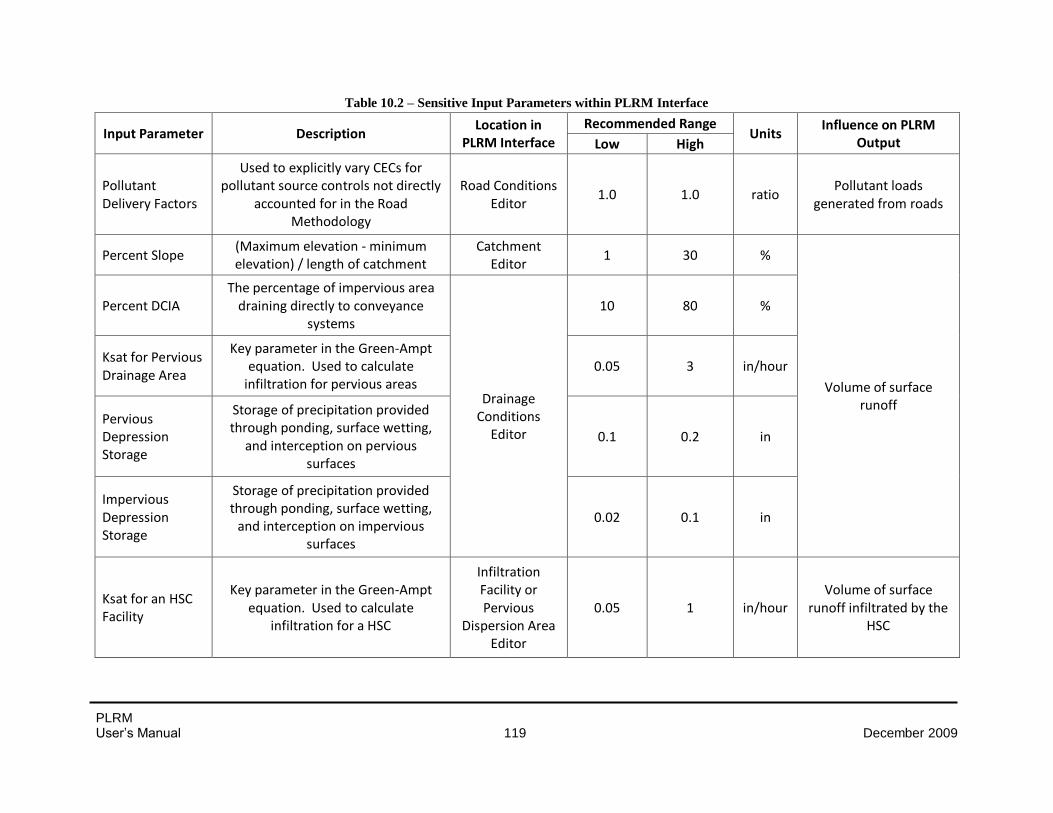
PLRM User’s Manual 119 December 2009
Table 10.2 – Sensitive Input Parameters within PLRM Interface
Input Parameter Description Location in
PLRM Interface Recommended Range
Units Influence on PLRM
Output Low High
Pollutant Delivery Factors
Used to explicitly vary CECs for pollutant source controls not directly
accounted for in the Road Methodology
Road Conditions Editor
1.0 1.0 ratio Pollutant loads
generated from roads
Percent Slope (Maximum elevation - minimum elevation) / length of catchment
Catchment Editor
1 30 %
Volume of surface runoff
Percent DCIA The percentage of impervious area
draining directly to conveyance systems
Drainage Conditions
Editor
10 80 %
Ksat for Pervious Drainage Area
Key parameter in the Green-Ampt equation. Used to calculate
infiltration for pervious areas 0.05 3 in/hour
Pervious Depression Storage
Storage of precipitation provided through ponding, surface wetting,
and interception on pervious surfaces
0.1 0.2 in
Impervious Depression Storage
Storage of precipitation provided through ponding, surface wetting,
and interception on impervious surfaces
0.02 0.1 in
Ksat for an HSC Facility
Key parameter in the Green-Ampt equation. Used to calculate
infiltration for a HSC
Infiltration Facility or Pervious
Dispersion Area Editor
0.05 1 in/hour Volume of surface
runoff infiltrated by the HSC
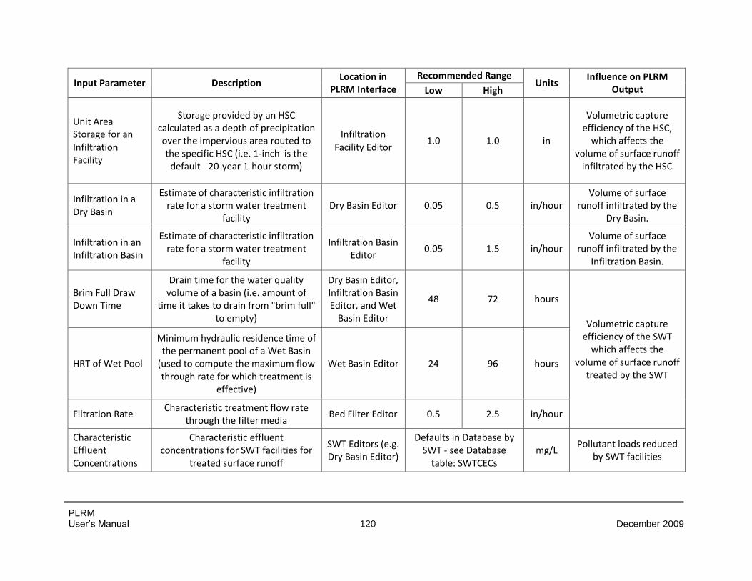
PLRM User’s Manual 120 December 2009
Input Parameter Description Location in
PLRM Interface Recommended Range
Units Influence on PLRM
Output Low High
Unit Area Storage for an Infiltration Facility
Storage provided by an HSC calculated as a depth of precipitation over the impervious area routed to the specific HSC (i.e. 1-inch is the
default - 20-year 1-hour storm)
Infiltration Facility Editor
1.0 1.0 in
Volumetric capture efficiency of the HSC,
which affects the volume of surface runoff
infiltrated by the HSC
Infiltration in a Dry Basin
Estimate of characteristic infiltration rate for a storm water treatment
facility Dry Basin Editor 0.05 0.5 in/hour
Volume of surface runoff infiltrated by the
Dry Basin.
Infiltration in an Infiltration Basin
Estimate of characteristic infiltration rate for a storm water treatment
facility
Infiltration Basin Editor
0.05 1.5 in/hour Volume of surface
runoff infiltrated by the Infiltration Basin.
Brim Full Draw Down Time
Drain time for the water quality volume of a basin (i.e. amount of
time it takes to drain from "brim full" to empty)
Dry Basin Editor, Infiltration Basin Editor, and Wet
Basin Editor
48 72 hours
Volumetric capture efficiency of the SWT
which affects the volume of surface runoff
treated by the SWT HRT of Wet Pool
Minimum hydraulic residence time of the permanent pool of a Wet Basin
(used to compute the maximum flow through rate for which treatment is
effective)
Wet Basin Editor 24 96 hours
Filtration Rate Characteristic treatment flow rate
through the filter media Bed Filter Editor 0.5 2.5 in/hour
Characteristic Effluent Concentrations
Characteristic effluent concentrations for SWT facilities for
treated surface runoff
SWT Editors (e.g. Dry Basin Editor)
Defaults in Database by SWT - see Database
table: SWTCECs mg/L
Pollutant loads reduced by SWT facilities
PLRM User’s Manual 121 December 2009
Pollutant Delivery Factors
Flagged As: Warning
Range: Low = 1.0; High = 1.0
Message: The Pollutant Delivery Factors provide a method to adjust the quantity of
pollutants of concern delivered to the outlet of the catchment. This option
was incorporated recognizing that the Road Methodology does not
account for every PSC action that may be implemented to improve runoff
quality. Values other than 1 are acceptable as Pollutant Delivery Factors,
but are flagged because the user should provide justification to project
reviewers when Pollutant Delivery Factors other than 1 are used. The
Pollutant Delivery Factors adjust the CRCs for pollutants of concern.
Reference: No specific reference is cited. Pollutant Delivery Factors are an internal
algorithm implemented in the PLRM to provide a flexible and transparent
process for adjusting CRCs if the Road Methodology is not deemed to be
sufficient to represent PSCs for roads.
Guidance: Developing the rationale and justification for using a Pollutant Delivery
Factor other than 1 is the responsibility of the user.

PLRM User’s Manual 122 December 2009
Average Slope
Flagged As: Warning
Range: Low = 1%; High = 30%
Message: The average slope is bounded by a recommended range to ensure the user
has entered a reasonable value. Values outside the recommended range
will be rare for Tahoe Basin urban areas and the user should double-check
their calculation of average slope.
Reference: The recommended range was developed based on review of calculations
of slopes for Tahoe Basin urban areas using a GIS analysis of the Tahoe
Basin Digital Elevation Model (DEM) available for download at:
http://tahoe.usgs.gov/DEM.html
Guidance: The calculation of average slope only needs to provide a representative
value for a user-defined catchment. A high level of accuracy is not
required. In most cases, the following calculation will suffice for average
slope = (maximum catchment elevation - minimum catchment elevation) /
length of catchment. If a significant grade break is evident in the
catchment (e.g. half the catchment is a 20% slope and the other half is 2%
slope), the user may want to consider modeling two separate catchments.
PLRM User’s Manual 123 December 2009
Percentage DCIA
Flagged As: Note
Range: Low = 10%; High = 80%
Message: The percentage of directly connected impervious area (DCIA) defined by
the user can significantly affect runoff volumes. Given the significance of
this parameter, values entered by the user for % DCIA outside the
recommended range are flagged. The message is only categorized as a
“Note” because values outside the recommended range can be a common
occurrence.
Reference: No specific reference is cited. The recommended range was developed to
highlight values entered by the user that indicate the impervious area is
either highly connected or highly disconnected. When a user enters a
value that is below the recommended minimum, the user has defined the
impervious area to be almost entirely disconnected (i.e. <10% DCIA).
When a user enters a value that is above the recommended maximum, the
user has defined the impervious are to be almost entirely connected (i.e.
>80% DCIA).
Guidance: The most current guidance for estimating the percentage of DCIA is found
in: Interim Guidance Paper for Formulating and Evaluating Alternatives
for Tahoe Basin Water Quality Improvement Projects (2008). That
Interim Guidance Paper can be downloaded at
http://www.trpa.org/default.aspx?tabindex=4&tabid=168
Figure 11.1 below is taken directly from the Interim Guidance Paper.
However, the complete guidance for estimating DCIA as described in the
Interim Guidance Paper is not repeated here.
Directly Connected Impervious Area (DCIA) - impervious surfaces
draining to conveyance systems via a hydraulic connection; Area A in
Figure 11.1.
Indirectly Connected Impervious Area (ICIA) – impervious surfaces
draining to pervious surfaces that promote infiltration, distribution and
energy dissipation, or storage prior to overflow draining to a conveyance
system; Area B in Figure 11.1.
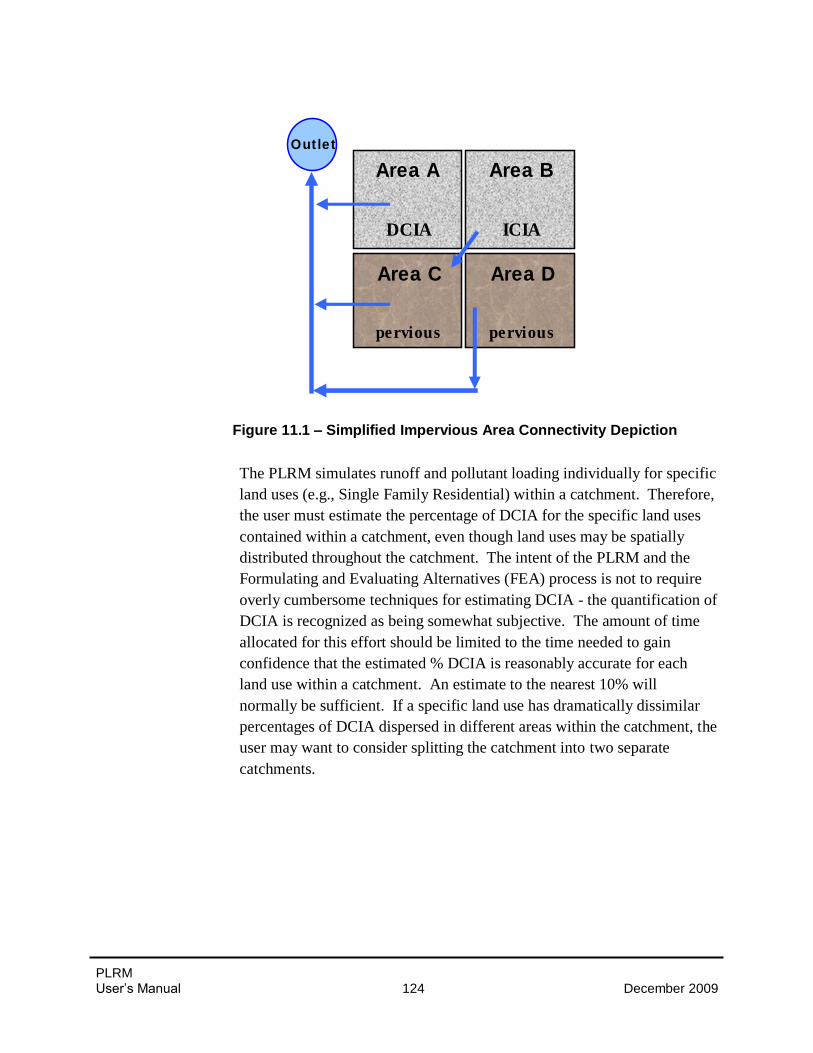
PLRM User’s Manual 124 December 2009
Figure 11.1 – Simplified Impervious Area Connectivity Depiction
The PLRM simulates runoff and pollutant loading individually for specific
land uses (e.g., Single Family Residential) within a catchment. Therefore,
the user must estimate the percentage of DCIA for the specific land uses
contained within a catchment, even though land uses may be spatially
distributed throughout the catchment. The intent of the PLRM and the
Formulating and Evaluating Alternatives (FEA) process is not to require
overly cumbersome techniques for estimating DCIA - the quantification of
DCIA is recognized as being somewhat subjective. The amount of time
allocated for this effort should be limited to the time needed to gain
confidence that the estimated % DCIA is reasonably accurate for each
land use within a catchment. An estimate to the nearest 10% will
normally be sufficient. If a specific land use has dramatically dissimilar
percentages of DCIA dispersed in different areas within the catchment, the
user may want to consider splitting the catchment into two separate
catchments.
Area A
DCIA
Area B
ICIA
Area D
pervious
Area C
pervious
Outlet
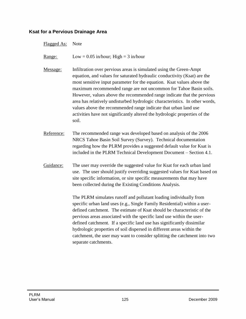
PLRM User’s Manual 125 December 2009
Ksat for a Pervious Drainage Area
Flagged As: Note
Range: Low = 0.05 in/hour; High = 3 in/hour
Message: Infiltration over pervious areas is simulated using the Green-Ampt
equation, and values for saturated hydraulic conductivity (Ksat) are the
most sensitive input parameter for the equation. Ksat values above the
maximum recommended range are not uncommon for Tahoe Basin soils.
However, values above the recommended range indicate that the pervious
area has relatively undisturbed hydrologic characteristics. In other words,
values above the recommended range indicate that urban land use
activities have not significantly altered the hydrologic properties of the
soil.
Reference: The recommended range was developed based on analysis of the 2006
NRCS Tahoe Basin Soil Survey (Survey). Technical documentation
regarding how the PLRM provides a suggested default value for Ksat is
included in the PLRM Technical Development Document – Section 4.1.
Guidance: The user may override the suggested value for Ksat for each urban land
use. The user should justify overriding suggested values for Ksat based on
site specific information, or site specific measurements that may have
been collected during the Existing Conditions Analysis.
The PLRM simulates runoff and pollutant loading individually from
specific urban land uses (e.g., Single Family Residential) within a user-
defined catchment. The estimate of Ksat should be characteristic of the
pervious areas associated with the specific land use within the user-
defined catchment. If a specific land use has significantly dissimilar
hydrologic properties of soil dispersed in different areas within the
catchment, the user may want to consider splitting the catchment into two
separate catchments.
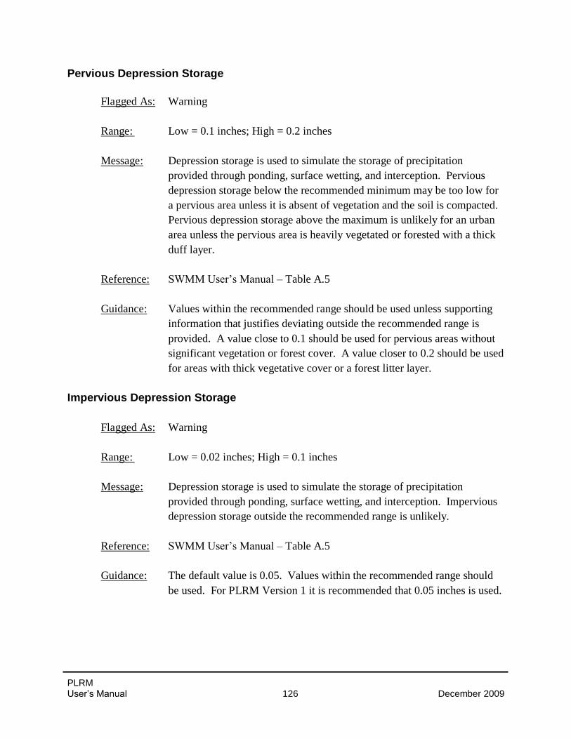
PLRM User’s Manual 126 December 2009
Pervious Depression Storage
Flagged As: Warning
Range: Low = 0.1 inches; High = 0.2 inches
Message: Depression storage is used to simulate the storage of precipitation
provided through ponding, surface wetting, and interception. Pervious
depression storage below the recommended minimum may be too low for
a pervious area unless it is absent of vegetation and the soil is compacted.
Pervious depression storage above the maximum is unlikely for an urban
area unless the pervious area is heavily vegetated or forested with a thick
duff layer.
Reference: SWMM User’s Manual – Table A.5
Guidance: Values within the recommended range should be used unless supporting
information that justifies deviating outside the recommended range is
provided. A value close to 0.1 should be used for pervious areas without
significant vegetation or forest cover. A value closer to 0.2 should be used
for areas with thick vegetative cover or a forest litter layer.
Impervious Depression Storage
Flagged As: Warning
Range: Low = 0.02 inches; High = 0.1 inches
Message: Depression storage is used to simulate the storage of precipitation
provided through ponding, surface wetting, and interception. Impervious
depression storage outside the recommended range is unlikely.
Reference: SWMM User’s Manual – Table A.5
Guidance: The default value is 0.05. Values within the recommended range should
be used. For PLRM Version 1 it is recommended that 0.05 inches is used.
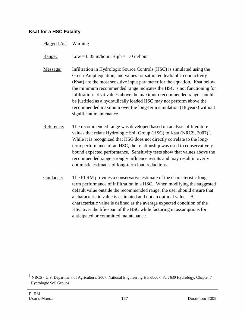
PLRM User’s Manual 127 December 2009
Ksat for a HSC Facility
Flagged As: Warning
Range: Low = 0.05 in/hour; High = 1.0 in/hour
Message: Infiltration in Hydrologic Source Controls (HSC) is simulated using the
Green-Ampt equation, and values for saturated hydraulic conductivity
(Ksat) are the most sensitive input parameter for the equation. Ksat below
the minimum recommended range indicates the HSC is not functioning for
infiltration. Ksat values above the maximum recommended range should
be justified as a hydraulically loaded HSC may not perform above the
recommended maximum over the long-term simulation (18 years) without
significant maintenance.
Reference: The recommended range was developed based on analysis of literature
values that relate Hydrologic Soil Group (HSG) to Ksat (NRCS, 2007)1.
While it is recognized that HSG does not directly correlate to the long-
term performance of an HSC, the relationship was used to conservatively
bound expected performance. Sensitivity tests show that values above the
recommended range strongly influence results and may result in overly
optimistic estimates of long-term load reductions.
Guidance: The PLRM provides a conservative estimate of the characteristic long-
term performance of infiltration in a HSC. When modifying the suggested
default value outside the recommended range, the user should ensure that
a characteristic value is estimated and not an optimal value. A
characteristic value is defined as the average expected condition of the
HSC over the life-span of the HSC while factoring in assumptions for
anticipated or committed maintenance.
1 NRCS - U.S. Department of Agriculture. 2007. National Engineering Handbook, Part 630 Hydrology, Chapter 7
Hydrologic Soil Groups.

PLRM User’s Manual 128 December 2009
Unit Area Storage for an Infiltration Facility
Flagged As: Note
Range: Low = 1.0 inch/impervious area; High = 1.0 inch/impervious area
Message: Current TRPA regulations require containment, at a minimum, of the
storm water runoff volume generated by a 20-year return period, 1-hour
duration “design storm” from impervious surfaces. The calculation of
runoff volume is made by multiplying the intensity of the 20-year 1-hour
design storm (taken as one inch of precipitation in one hour) by the
impervious surface area. A value other than 1 inch indicates the user is
evaluating an infiltration facility that is sized for a runoff volume
generated by something other than one inch of precipitation (i.e. the
current design storm). The minimum and maximum values for the
recommended range were both set to 1 inch to flag when the user is
evaluating an alternative design sizing criteria for an HSC.
Reference: Based on TRPA regulations for the 20-year 1-hour storm, which equates
to 1 inch of precipitation over the impervious drainage area.
Guidance: The PLRM allows the user to adjust the sizing criterion for an Infiltration
Facility by adjusting the unit area storage value. This may be useful to
evaluate situations where Infiltration Facilities cannot be sized to store the
20-year 1-hour storm because of physical constraints. For example, it’s
common for water quality improvement projects on roads to store less
than the 20-year 1-hour storm volume because of constraints in road
rights-of-way that limit storage opportunities.
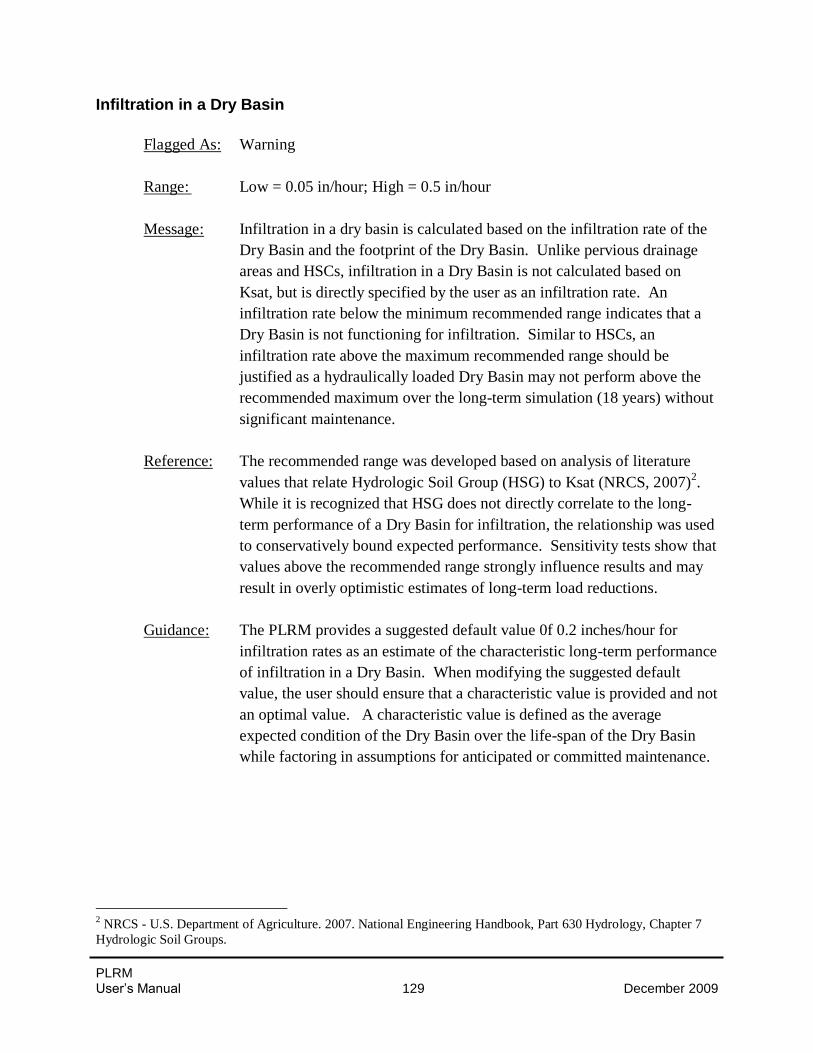
PLRM User’s Manual 129 December 2009
Infiltration in a Dry Basin
Flagged As: Warning
Range: Low = 0.05 in/hour; High = 0.5 in/hour
Message: Infiltration in a dry basin is calculated based on the infiltration rate of the
Dry Basin and the footprint of the Dry Basin. Unlike pervious drainage
areas and HSCs, infiltration in a Dry Basin is not calculated based on
Ksat, but is directly specified by the user as an infiltration rate. An
infiltration rate below the minimum recommended range indicates that a
Dry Basin is not functioning for infiltration. Similar to HSCs, an
infiltration rate above the maximum recommended range should be
justified as a hydraulically loaded Dry Basin may not perform above the
recommended maximum over the long-term simulation (18 years) without
significant maintenance.
Reference: The recommended range was developed based on analysis of literature
values that relate Hydrologic Soil Group (HSG) to Ksat (NRCS, 2007)2.
While it is recognized that HSG does not directly correlate to the long-
term performance of a Dry Basin for infiltration, the relationship was used
to conservatively bound expected performance. Sensitivity tests show that
values above the recommended range strongly influence results and may
result in overly optimistic estimates of long-term load reductions.
Guidance: The PLRM provides a suggested default value 0f 0.2 inches/hour for
infiltration rates as an estimate of the characteristic long-term performance
of infiltration in a Dry Basin. When modifying the suggested default
value, the user should ensure that a characteristic value is provided and not
an optimal value. A characteristic value is defined as the average
expected condition of the Dry Basin over the life-span of the Dry Basin
while factoring in assumptions for anticipated or committed maintenance.
2 NRCS - U.S. Department of Agriculture. 2007. National Engineering Handbook, Part 630 Hydrology, Chapter 7
Hydrologic Soil Groups.
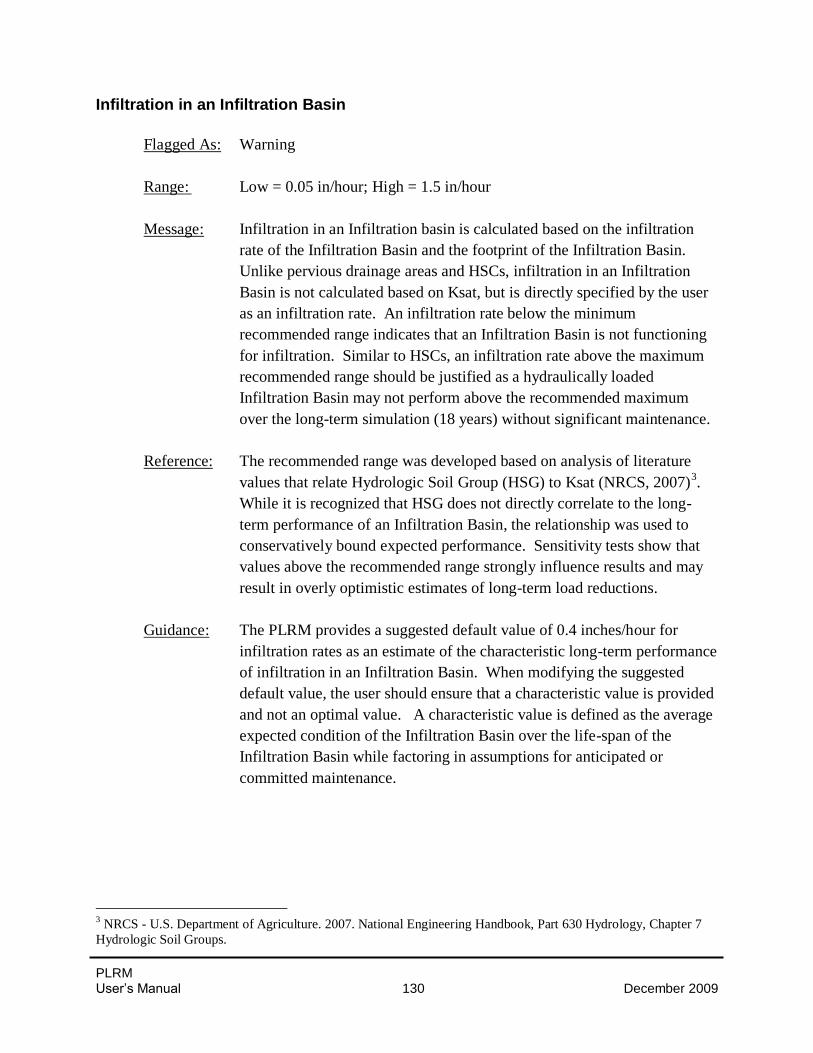
PLRM User’s Manual 130 December 2009
Infiltration in an Infiltration Basin
Flagged As: Warning
Range: Low = 0.05 in/hour; High = 1.5 in/hour
Message: Infiltration in an Infiltration basin is calculated based on the infiltration
rate of the Infiltration Basin and the footprint of the Infiltration Basin.
Unlike pervious drainage areas and HSCs, infiltration in an Infiltration
Basin is not calculated based on Ksat, but is directly specified by the user
as an infiltration rate. An infiltration rate below the minimum
recommended range indicates that an Infiltration Basin is not functioning
for infiltration. Similar to HSCs, an infiltration rate above the maximum
recommended range should be justified as a hydraulically loaded
Infiltration Basin may not perform above the recommended maximum
over the long-term simulation (18 years) without significant maintenance.
Reference: The recommended range was developed based on analysis of literature
values that relate Hydrologic Soil Group (HSG) to Ksat (NRCS, 2007)3.
While it is recognized that HSG does not directly correlate to the long-
term performance of an Infiltration Basin, the relationship was used to
conservatively bound expected performance. Sensitivity tests show that
values above the recommended range strongly influence results and may
result in overly optimistic estimates of long-term load reductions.
Guidance: The PLRM provides a suggested default value of 0.4 inches/hour for
infiltration rates as an estimate of the characteristic long-term performance
of infiltration in an Infiltration Basin. When modifying the suggested
default value, the user should ensure that a characteristic value is provided
and not an optimal value. A characteristic value is defined as the average
expected condition of the Infiltration Basin over the life-span of the
Infiltration Basin while factoring in assumptions for anticipated or
committed maintenance.
3 NRCS - U.S. Department of Agriculture. 2007. National Engineering Handbook, Part 630 Hydrology, Chapter 7
Hydrologic Soil Groups.
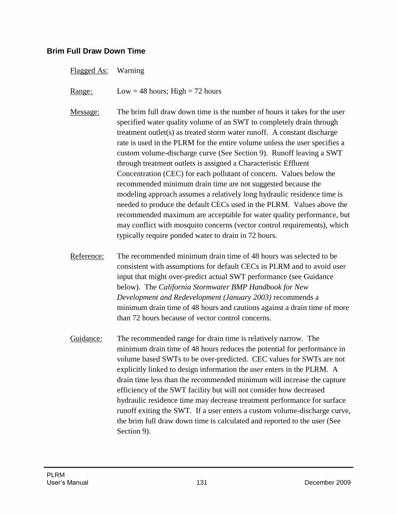
PLRM User’s Manual 131 December 2009
Brim Full Draw Down Time
Flagged As: Warning
Range: Low = 48 hours; High = 72 hours
Message: The brim full draw down time is the number of hours it takes for the user
specified water quality volume of an SWT to completely drain through
treatment outlet(s) as treated storm water runoff. A constant discharge
rate is used in the PLRM for the entire volume unless the user specifies a
custom volume-discharge curve (See Section 9). Runoff leaving a SWT
through treatment outlets is assigned a Characteristic Effluent
Concentration (CEC) for each pollutant of concern. Values below the
recommended minimum drain time are not suggested because the
modeling approach assumes a relatively long hydraulic residence time is
needed to produce the default CECs used in the PLRM. Values above the
recommended maximum are acceptable for water quality performance, but
may conflict with mosquito concerns (vector control requirements), which
typically require ponded water to drain in 72 hours.
Reference: The recommended minimum drain time of 48 hours was selected to be
consistent with assumptions for default CECs in PLRM and to avoid user
input that might over-predict actual SWT performance (see Guidance
below). The California Stormwater BMP Handbook for New
Development and Redevelopment (January 2003) recommends a
minimum drain time of 48 hours and cautions against a drain time of more
than 72 hours because of vector control concerns.
Guidance: The recommended range for drain time is relatively narrow. The
minimum drain time of 48 hours reduces the potential for performance in
volume based SWTs to be over-predicted. CEC values for SWTs are not
explicitly linked to design information the user enters in the PLRM. A
drain time less than the recommended minimum will increase the capture
efficiency of the SWT facility but will not consider how decreased
hydraulic residence time may decrease treatment performance for surface
runoff exiting the SWT. If a user enters a custom volume-discharge curve,
the brim full draw down time is calculated and reported to the user (See
Section 9).
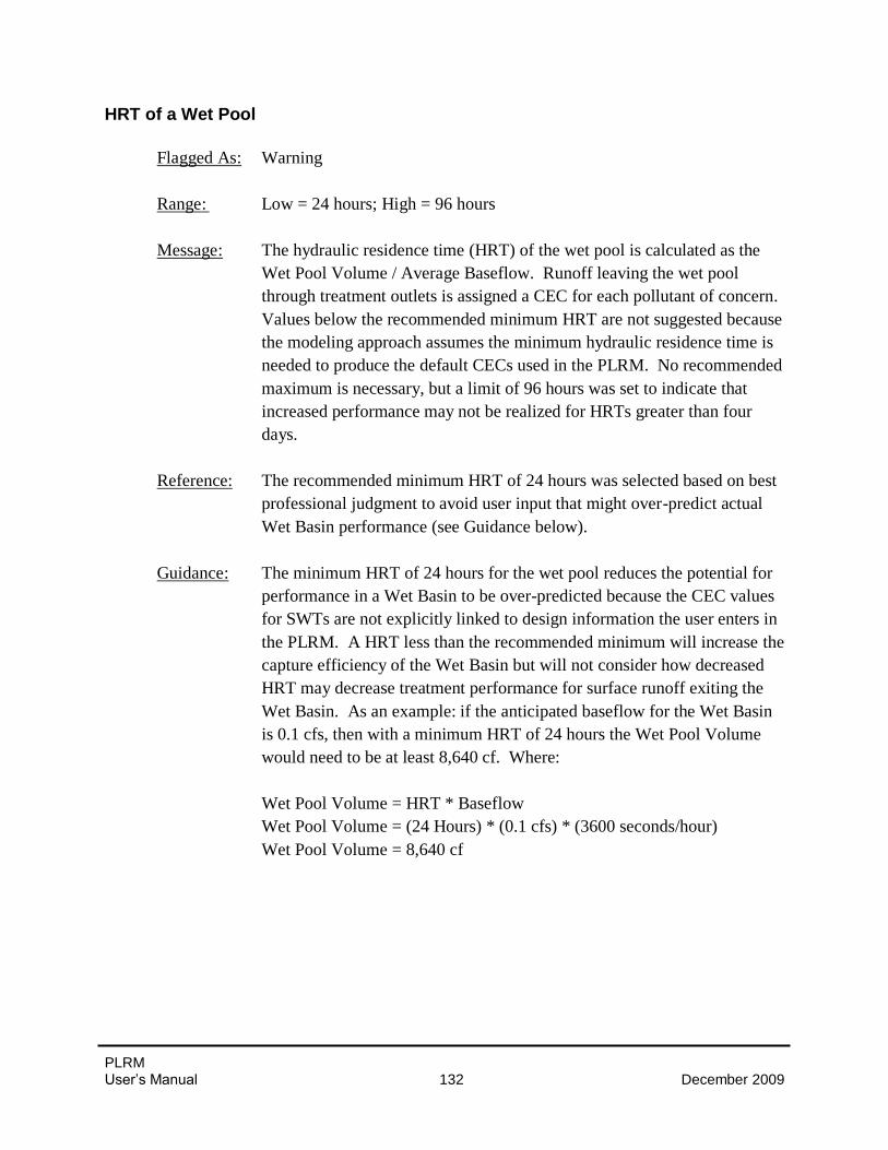
PLRM User’s Manual 132 December 2009
HRT of a Wet Pool
Flagged As: Warning
Range: Low = 24 hours; High = 96 hours
Message: The hydraulic residence time (HRT) of the wet pool is calculated as the
Wet Pool Volume / Average Baseflow. Runoff leaving the wet pool
through treatment outlets is assigned a CEC for each pollutant of concern.
Values below the recommended minimum HRT are not suggested because
the modeling approach assumes the minimum hydraulic residence time is
needed to produce the default CECs used in the PLRM. No recommended
maximum is necessary, but a limit of 96 hours was set to indicate that
increased performance may not be realized for HRTs greater than four
days.
Reference: The recommended minimum HRT of 24 hours was selected based on best
professional judgment to avoid user input that might over-predict actual
Wet Basin performance (see Guidance below).
Guidance: The minimum HRT of 24 hours for the wet pool reduces the potential for
performance in a Wet Basin to be over-predicted because the CEC values
for SWTs are not explicitly linked to design information the user enters in
the PLRM. A HRT less than the recommended minimum will increase the
capture efficiency of the Wet Basin but will not consider how decreased
HRT may decrease treatment performance for surface runoff exiting the
Wet Basin. As an example: if the anticipated baseflow for the Wet Basin
is 0.1 cfs, then with a minimum HRT of 24 hours the Wet Pool Volume
would need to be at least 8,640 cf. Where:
Wet Pool Volume = HRT * Baseflow
Wet Pool Volume = (24 Hours) * (0.1 cfs) * (3600 seconds/hour)
Wet Pool Volume = 8,640 cf
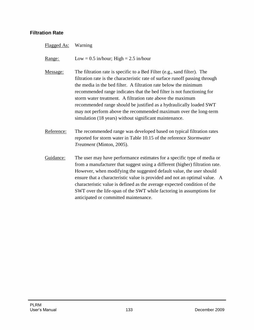
PLRM User’s Manual 133 December 2009
Filtration Rate
Flagged As: Warning
Range: Low = 0.5 in/hour; High = 2.5 in/hour
Message: The filtration rate is specific to a Bed Filter (e.g., sand filter). The
filtration rate is the characteristic rate of surface runoff passing through
the media in the bed filter. A filtration rate below the minimum
recommended range indicates that the bed filter is not functioning for
storm water treatment. A filtration rate above the maximum
recommended range should be justified as a hydraulically loaded SWT
may not perform above the recommended maximum over the long-term
simulation (18 years) without significant maintenance.
Reference: The recommended range was developed based on typical filtration rates
reported for storm water in Table 10.15 of the reference Stormwater
Treatment (Minton, 2005).
Guidance: The user may have performance estimates for a specific type of media or
from a manufacturer that suggest using a different (higher) filtration rate.
However, when modifying the suggested default value, the user should
ensure that a characteristic value is provided and not an optimal value. A
characteristic value is defined as the average expected condition of the
SWT over the life-span of the SWT while factoring in assumptions for
anticipated or committed maintenance.
PLRM User’s Manual 134 December 2009
Characteristic Effluent Concentration
Flagged As: Warning
Range: Defaults depend on the type of SWT and pollutant of concern.
Message: Characteristic Effluent Concentrations (CECs) were developed through a
statistical analysis of storm water performance data to predict a
representative level of treatment for each type of SWT facility included in
the PLRM. Modification to CECs values should be justified by the user
and the program will flag any value for any pollutant of concern that
deviates from the default value.
Reference: The development of the existing default CEC values for each type of SWT
facility included in the PLRM are described in the PLRM Model
Development Document – Section 7.2.
Guidance: The PLRM provides suggested default CEC values. As noted in
Section 7.2 of the Model Development Documentation, additional work is
needed and is underway to improve the default CEC values. The current
CEC values are based on a statistical analysis of best available data from
multiple storm water performance studies for each type of SWT facility
included in the PLRM. The statistical nature of the analysis is assumed to
provide a representative performance estimate for each SWT facility.
Justification should be provided if the default CEC values are replaced
using data from a single storm water performance study. For example, if
the design of the proposed facility is very similar to the design of a
monitored facility the performance of the two may be expected to be
comparable assuming similar drainage characteristics and climatic
conditions. However, the user should be cautious about using data from
relatively short term studies.
PLRM User’s Manual 135 December 2009
11.0 PLRM Database Overview The PLRM Database is a Microsoft Access 2007 database used to 1) store Default Parameters
and preprocessed input data; 2) store program configurations; and 3) dynamically generate
several PLRM Interface components and Input Parameters based on user entry. The PLRM
Database significantly reduces the data preparation and data input burden on the user relative to
typical requirements for building a continuous simulation model of hydrology and pollutant
loading. The typical user of the PLRM does not need to interact directly with the PLRM
Database.
The PLRM Database was designed to provide an application that is simple to use, while allowing
flexibility for future database modifications or additions. The database structure was developed
to dynamically interact with the PLRM Interface so that future updates or modifications to
PLRM Database are reflected in the PLRM without the need to redesign and recompile the
program. Note that as discussed in the previous section, the Default Parameters included within
the PLRM Database are not recommended for modification by the user unless the modifications
are done to incorporate new or additional data. Maintaining consistent Default Parameters in the
PLRM Database is recommended because it will help to maintain consistency of results
generated by multiple user’s across multiple project areas.
During the installation process for the PLRM, the PLRM
Database is unpacked and saved into the Data Directory
with a filename of: PLRMv1.0.accdb. The PLRM
Database was built in Microsoft Access 2007 and a user
needs to have Microsoft Access 2007 installed on their
computer to view the PLRM Database. However,
Microsoft Access 2007 does not need to be installed on
a user’s computer to run the PLRM. The PLRM setup
program includes the free software: Microsoft Access
Runtime 2007 (Runtime). The PLRM setup program
will install Runtime on a user’s computer to ensure the
PLRM successfully interacts with the PLRM Database
regardless of the presence of Microsoft Access 2007.
Figure 11.1 illustrates the function of the PLRM Database within the overall PLRM program
structure. The PLRM Input Forms interact with the PLRM Database to automate many of the
data entry needs required for a simulation. Besides the storage of Default Parameters, the PLRM
Database executes technical algorithms on certain data sets to generate required data entry based
on user entry in the PLRM Input Forms. For example, location specific meteorological data sets
are created from the PLRM Database based on the meteorological grid cell the user defines in the
Project Editor.
Key Concept Box
A user needs to have Microsoft
Access 2007 installed on their
computer to view the PLRM
Database. However, Microsoft
Access 2007 does not need to be
installed to run the PLRM. The
PLRM setup program includes
the free software: Microsoft
Access Runtime 2007 (Runtime)
to ensure the PLRM successfully
interacts with the PLRM
Database.
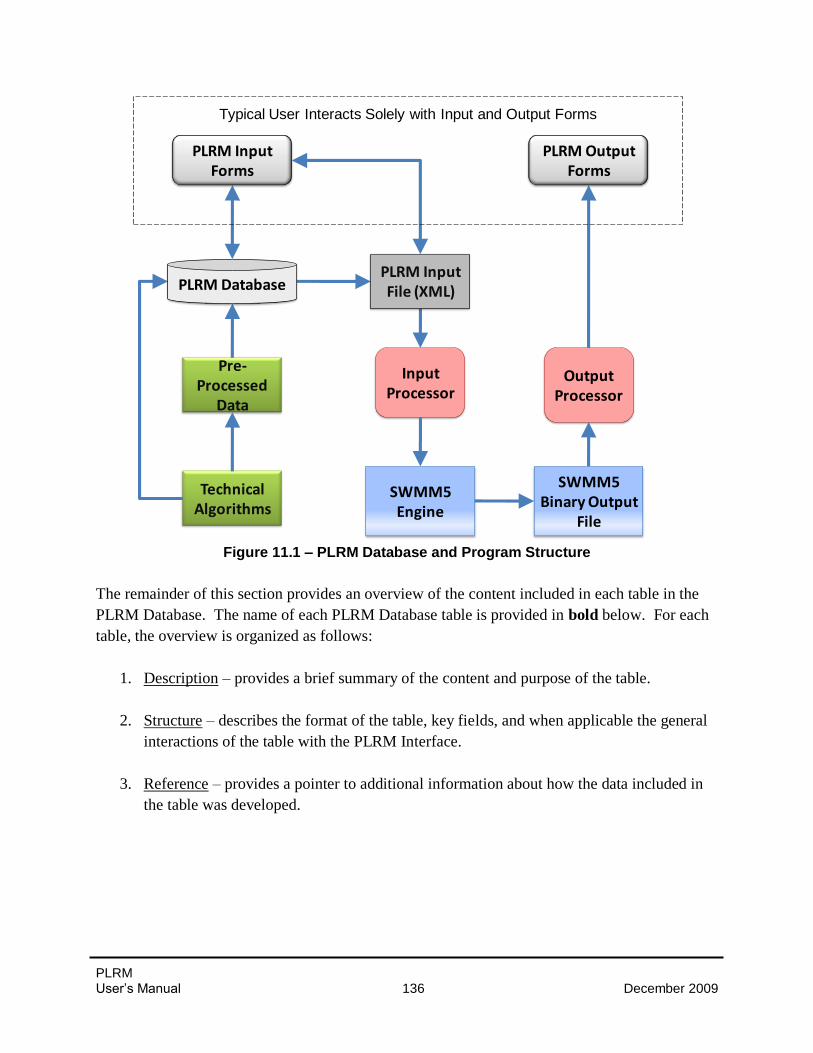
PLRM User’s Manual 136 December 2009
Figure 11.1 – PLRM Database and Program Structure
The remainder of this section provides an overview of the content included in each table in the
PLRM Database. The name of each PLRM Database table is provided in bold below. For each
table, the overview is organized as follows:
1. Description – provides a brief summary of the content and purpose of the table.
2. Structure – describes the format of the table, key fields, and when applicable the general
interactions of the table with the PLRM Interface.
3. Reference – provides a pointer to additional information about how the data included in
the table was developed.
SWMM5 Engine
Pre-Processed
Data
PLRM Input Forms
Input Processor
Technical Algorithms
Output Processor
SWMM5 Binary Output
File
PLRM DatabasePLRM Input File (XML)
PLRM Output Forms
Typical User Interacts Solely with Input and Output Forms

PLRM User’s Manual 137 December 2009
ArealDepletion
Description: Values in this table are used to specify points on Areal Depletion Curves for both
impervious and pervious surfaces. Areal depletion refers to the tendency of accumulated snow
to melt non-uniformly. Each curve is defined by 10 equal increments of a relative depth ratio
between 0 and 0.9, where a relative depth ratio is an area's current snow depth divided by the
depth at which there is 100% areal coverage.
Structure: The table includes two rows that define Areal Depletion Curves separately for
impervious and pervious surfaces in 10 equal increments.
Reference: Values in the PLRM Database are default values used by SWMM5 for natural areas.
Additional discussion of Areal Depletion Curves can be found in the SWMM5 User’s Manual:
http://www.epa.gov/ednnrmrl/models/swmm/
Aquifer
Description: Values in this table are used calculate transpiration and to define the groundwater
elevation at the start of the simulation.
Structure: The table includes one row and a number of columns organized to inform the
SWMM5 code for Aquifers. A number of fields are blank in the table because an algorithm is
used to populate the fields based on the meteorological grid cell the user defines in the Project
Editor. A description of each field can be reviewed by opening the table in Design View in
Access.
Reference: Section 4.2 of the Model Development Document.
BuildupParcels
Description: The table includes SWMM5 code required to simulate buildup of pollutants for
each land use and associated pollutant of concern. Because the PLRM does not use SWMM5
algorithms to simulate the buildup of pollutants, all values in this table are zero.
Structure: A description of each field can be reviewed by opening the table in Design View in
Access.
Reference: None cited. Pollutant buildup is not simulated in the PLRM but the code is
transferred from the PLRM Database to the SWMM5 input file to ensure the SWMM5
simulation executes correctly.
PLRM User’s Manual 138 December 2009
CatchmentValidationRules Description: The table includes default recommended ranges for key Input Parameters that are
associated with data entry for defining the properties of a catchment.
Structure: Values in Min and Max columns are used by the Recommended Range Report to
flag user entered values that are outside the Min or Max value. The Flag column categorizes the
type of message that will be generated as a Note, Warning, or Error.
Reference: See Section 10.2 of this Manual.
Codes Description: This is the primary table used within the PLRM Database to relate internal fields
and to define fields. The PLRM Database uses values in the codes column to relate to most other
fields in the PLRM Database.
Structure: This is the primary table used to define a new field for land uses, pollutants of
concern, SWT facilities, etc. The following are functions of the columns in the table:
code – value used by the PLRM Database to define a field
name – name of field
PLRM_Name – abbreviation used in XML code to generate a SWMM5 input file
description – describes how a specific code fits within a family of codes
Reference: None cited; this is the internal reference table for the PLRM Database.
Defaults
Description: The table includes various defaults used in the PLRM Interface and some values
used by database algorithms. This table also includes land use specific compaction factors used
in the algorithm that generates recommended values for Ksat that appear in the Drainage
Conditions Editor. Land use specific compaction factors have IDs in the 700s for this table.
Structure: The following are functions of key columns in this table:
defaultValue – the value used by the PLRM Interface for a specific variable
description – a brief description of where the default value is used
variable – a brief description of the variable
Reference: See Section 10.2 of this Manual for a discussion on the various default values. See
Section 4.1 of the Model Development Document for discussion on how compaction factors are
applied to generate recommended Ksat values.
PLRM User’s Manual 139 December 2009
Evaporation Description: This table includes daily evaporation rates in inches per day organized as monthly
normals. Evaporation rates are used to calculate evaporation and transpiration over the
simulation period.
Structure: Evaporation rates are input as monthly normals in units of inches/day.
Reference: See Section 4.4 of the Model Development Document.
Groundwater
Description: Values for parameters in this table are used to compute rate of groundwater flow,
which affects computations that determine the volume of infiltrated runoff that percolates to
groundwater relative to the amount that is transpired.
Structure: The table includes one row and a number of columns formatted in a manner to inform
the SWMM5 code. A description of each field can be reviewed by opening the table in Design
View in Access.
Reference: See Section 4.2 of the Model Development Document.
HydSoilGroup
Description: This table relates hydrologic soil group to soil suction head.
Structure: The table is used with the Soils table to provide a value for soil suction head for the
Green-Ampt equation in the SWMM5 code used to compute infiltration. Hydrologic soil group
is defined based on user entry in the Soils Editor. The following are functions of key columns
in the table:
HSC – hydrologic soil group
SoilSuctionHead – the assigned soil suction head for the associated hydrologic soil group.
Reference: See Section 4.1 of the Model Development Document.
PLRM User’s Manual 140 December 2009
LandUseParcels Description: This table includes SWMM5 code required for each land use and associated
pollutant of concern to simulate street sweeping intervals. Because the PLRM uses external
algorithms to estimate the effectiveness of street sweeping, all values in this table are zero.
Structure: The table includes each unique land use in the PLRM. A description of each field can
be reviewed by opening the table in Design View in Access.
Reference: None cited. The SWMM5 algorithms for sweeping are not used in the PLRM but
the code is transferred from the PLRM Database to the SWMM5 input file to ensure the
SWMM5 simulation executes correctly.
LandUses
Description: This table includes TMDL land uses that will be selectable from Land Use Editor.
The table includes default values for the percentage of impervious area associated with each land
use that appear in the % Impervious field of the Land Use Editor.
Structure: Available land uses in the Land Use Editor are populated from this table. The
following are functions of key columns in the table:
code – value in the Codes table of the PLRM Database
name – name of land use
PLRM_Name – abbreviation used in XML code to generate a SWMM5 input file
defaultImpervFraction – default values that populate the % Impervious field of the
Land Use Editor
description – describes family of codes; land uses can be any code from 100-199
Reference: Default land uses included in the table are defined by the TMDL Land Use GIS
Layer, which can be downloaded from the Lahontan LRWQCB website:
http://www.waterboards.ca.gov/lahontan/water_issues/programs/tmdl/lake_tahoe/index.shtml

PLRM User’s Manual 141 December 2009
MetGrid Description: The table includes data sets for each meteorological grid cell used in the
meteorological extrapolation.
Structure: Each row in the table is a unique meteorological grid cell and includes the assigned
SnoTel gage; monthly scaling factors for precipitation; average elevation of the grid cell in the
Tahoe Basin; and a temperature adjustment based on the difference in elevation between the
assigned SnoTel gage and the average elevation of the grid cell. A description of each field can
be reviewed by opening the table in Design View in Access.
Reference: See Section 3 of the Model Development Document.
MonthlyWindSpeed
Description: This table includes the monthly average windspeed used by the heat budget
equation for SWMM5 to calculate snowmelt during periods with precipitation.
Structure: Wind speed values are input as monthly normal values in units of mph.
Reference: Default values are average values for the Tahoe Basin taken from the Fifth-
Generation Mesoscale Model (MM5), which was used by researchers at UCDavis to predict
meteorological variables for the Tahoe Basin.
nodeValidationRules
Description: The table includes default recommended ranges for key Input Parameters
associated with SWT facilities, as well as default recommended ranges for Characteristic
Effluent Concentrations (CECs) for each SWT facility.
Structure: Values in Min and Max columns are used by the Recommended Range Report to
flag user entered values outside the Min or Max value. The Flag column categorizes the type of
message that will be generated as a Note, Warning, or Error.
For CECs, the Min and Max values are equal in this table. This ensures that any value other than
the default CEC value will be flagged by the Recommended Range Report if CECs are
changed in the SWT Editors (e.g., Dry Basin Editor, Wet Basin Editor).
Reference: See Section 7.1 of the Model Development Document for more information on SWT
design parameters. See Section 7.2 of the Model Development Document for more information
on default CEC values.
PLRM User’s Manual 142 December 2009
Options Description: This table includes default values that standardize the parameters used to define a
PLRM Simulation relative to the various analysis options that can be performed in a SWMM5
simulation.
Structure: Each field in the Category column describes a SWMM5 analysis option. The
Parameter column is the value or option used for a PLRM simulation. The Start Date and End
Date fields are blank because these values are populated based on the user’s selection of either a
Short Simulation or Full Simulation from the Project Editor.
Reference: See Appendix D of the SWWM5 User’s Manual for a description of the various
analysis options for a SWMM5 simulation.
ParcelCRCs
Description: This table includes characteristic runoff concentrations (CRCs) for pollutants of
concern for all land uses not incorporated into the Road Methodology, which is all land uses in
the Parcel Methodology as well as all Erosion Potential land uses.
Structure: This table provides CRCs to the SWWM5 code for all land uses except Road Land
Uses, including Urban Land Uses with BMPs implemented. A description of each field can be
reviewed by opening the table in Design View in Access. The following are functions of key
columns in the table:
code – value in the Codes table for land uses
Pollutant_Code – value in the Codes table for pollutant of concern
Land_Use – abbreviation used in XML code to generate a SWMM5 input file
Pollutant – abbreviation for pollutant of concern
Function – SWWM5 analysis option, always “EMC”
Coeff1 – CRC for land use and pollutant of concern in units of mg/L
Reference: See Section 5.2 of the Model Development Document.
Pollutants
Description: This table defines pollutants of concern simulated by the PLRM.
Structure: The table includes a number of required fields needed by the SWMM5 code to define
each pollutant of concern. A description of each field can be reviewed by opening the table in
Design View in Access.
Reference: See Section 5.2 of the Model Development Document.
PLRM User’s Manual 143 December 2009
PrecipTimeSeries
Description: This table includes an 18-year data set (Water Year 1989 to 2006) of precipitation
for eight SnoTel gages in the Tahoe Basin. Data is provided as depth in inches on hourly
intervals. Data is only for hours when precipitation is recorded; SWMM 5 assumes missing
hours are periods without precipitation.
Structure: The columns in the table are formatted so the time series can be exported and read
directly as a SWMM5 input file for precipitation. The column SnoTelID is the code identifying
the SnoTel station. The column Precip is the depth of precipitation recorded at that SnoTel
station for the specific hour in units of inches.
Reference: See Section 3 of the Model Development Document.
RoadCRCs
Description: This table includes characteristic runoff concentrations (CRCs) for pollutants of
concern for Road Land Uses, which are related to the calculation of Pollutant Potential.
Pollutant Potential is determined through user input in the Road Conditions Editor and the
database table RoadPollutantPotential.
Structure: For each pollutant of concern, the table repeats Pollutant Potential scores in one-tenth
increments from 0.5 to 5. A CRC is assigned to each Pollutant Potential score for each pollutant
of concern. These CRC values are dynamically read into the Road Conditions Editor based on
the Pollutant Potential Score calculated by the Road Conditions Editor.
Reference: Section 5.1 and Appendix B of the Model Development Document describes how
CRCs were developed and related to Pollutant Potential scores for each pollutant of concern.
RoadPollutantPotential
Description: Values in this table are used to relate Road Risk, a road shoulder stabilization
score, and a road abrasive application score to a Pollutant Potential score.
Structure: The Road Conditions Editor interacts dynamically with this table to continuously
update Pollutant Potential based on user entry in the Road Conditions Editor. The PLRM
queries this table for: 1) Road Risk [column RdLandUseAndRisk]; 2) Road Stabilization Score
[RdStabScore]; and 3) Abrasive Application Score [column AbrAppScore] to return a unique
Pollutant Potential Score (column PollutantPotential). The Pollutant Potential score is related to
the CRCs in the table RoadCRCs.
Reference: See Section 5.1 and Appendix B of the Model Development Document describe how
Pollutant Potential relates to Road Risk, road shoulder stabilization, and abrasive applications.
PLRM User’s Manual 144 December 2009
Simulation Period
Description: This table defines the Start Date and End Date for a Short Simulation and Full
Simulation. The user selects the simulation period from the Project Editor.
Structure: The fields in this table are used to populate blank fields in the Options table based on
user entry in the Project Editor.
Reference: See Section 3.1 of this Manual. Snowmelt
Description: This table includes snowmelt parameters for the temperature index method used by
SWMM5 to compute snowmelt.
Structure: A description of each field can be reviewed by opening the table in Design View in
Access. The column ElevationAboveMSL is blank because the elevation is populated based on
the meteorological grid cell the user defines in the Project Editor. Elevation is read from the
MetGrid table.
Reference: See Section 4.3 of the Model Development Document.
Snowpacks
Description: This table includes snowmelt parameters for the temperature index method used by
SWMM5, as well as parameters used by the SWMM5 snow management algorithm.
Structure: The table includes values for minimum and maximum melt coefficients, snow
management coefficients, etc. Three separate snowmelt routines are included in the table. The
three separate snowmelt routines are applied as follows to land uses in the PLRM:
1. Roads – applied to Road Land Uses
2. Parcels – applied to Single-Family Residential, Multi-Family Residential, and CICU
3. Pervious – applied to all other land uses.
Each routine is organized in the formatting required by the SWMM5 code, which includes four
rows of data entry:
1. Row 1 defines the melt coefficient for plowable surfaces
2. Row 2 defines the melt coefficient for impervious surfaces not plowed
3. Row 3 defines the melt coefficient for pervious surfaces
4. Row 4 defines plowing characteristics.

PLRM User’s Manual 145 December 2009
A description of each field and each row used to populate the SWMM5 code can be reviewed by
opening the table in Design View in Access.
Reference: See Section 4.3 of the Model Development Document.
Soils
Description: This table includes hydrologic properties of soil for each Map Unit from the 2006
NRCS Tahoe Basin Soil Survey (Survey).
Structure: Available soils by Map Unit in the Soils Editor are populated from this table.
Additionally, this table is used to generate recommended values for Ksat that appear in the
Drainage Conditions Editor. The following are functions of key columns in the table:
MU – unique identifier for the Map Unit as defined by the Survey
HydSoilGroupID – the dominant hydrologic soil group of the Map Unit. This value is
related to the table HydSoilGroup to supply Soil Suction Head to the SWMM5 code for
the Green-Ampt equation
KsatPervoius – value taken from the Survey for saturated hydraulic conductivity (Ksat)
of the Map Unit in units of inches/hour
SoilMoisDef – initial soil moisture deficit of the Map Unit; value is used in the Green-
Amp equation in SWMM5
MUName – long description of the Map Unit
Reference: See Section 4.1 of the Model Development Document.
Sweeping Effectiveness
Description: This table provides default values that estimate the effectiveness of pollutant
recovery through street sweeping by sweeper type and sweeping frequency.
Structure: The Road Conditions Editor interacts dynamically with this table to continuously
update Sweeping Effectiveness based on user entry, which in turn adjusts CRCs in the Road
Conditions Editor. A description of each field can be reviewed by opening the table in Design
View in Access:
SweeperTypeScore – value in the column relates to the Codes table for the specific
sweeper type
SweepFrequencyScore –value in the column relates to the Codes table for the specific
sweeping strategy
PollutantCode – Pollutant code from the Codes table
Percent_Red – Percent reduction in CRC based on the combination of sweeper type and
sweeping strategy selected in the Road Conditions Editor for each pollutant of concern
PLRM User’s Manual 146 December 2009
Reference: Section 5.1 and Appendix B of the Model Development Document describe how
default street sweeping effectiveness values were developed.
SWTCECs
Description: The table includes default characteristic effluent concentrations (CECs) for each
SWT facility and pollutant of concern in the PLRM. Default values are use to populate CECs in
the SWT Editors (e.g., Dry Basin Editor, Wet Basin Editor)
Structure: A description of each field can be reviewed by opening the table in Design View in
Access; notable columns in the table include:
SWT_Code – value relates to the Codes table to define the specific SWT facility
CEC_Value – default CECs for each SWT facility and each pollutant of concern
Reference: See Section 7.2 of the Model Development Document.
SWTDesignParameters
Description: The table includes default design parameters organized by SWT facility. Default
values are used in the SWT Editors (e.g., Dry Basin Editor, Wet Basin Editor)
Structure: A description of each field can be reviewed by opening the table in Design View in
Access; notable columns in the table include:
SWT_Code – value in the column relates to the Codes table to define the specific SWT
facility
variable – description of design parameter
defaultValue – default value used by in the SWT Editors
Reference: See Section 7.1 of the Model Development Document.
TempTimeSeries
Description: This table includes an 18-year data set (Water Year 1989 to 2006) of temperature
for eight SnoTel gages in the Tahoe Basin. Data is provided in degrees Fahrenheit at hourly
intervals.
Structure: The columns in the table are formatted so the time series can be read exported and
read directly as a SWMM5 input file for temperature. The column SnoTelID is the code
identifying the SnoTel station. The column AirTemp is the temperature recorded at that SnoTel
station for the specific hour in degrees Fahrenheit.
Reference: See Section 3 of the Model Development Document.
PLRM User’s Manual 147 December 2009
12.0 Notes on PLRM Modeling
12.1 Limitations and Structure of Version 1
Catchment simulation size
The PLRM was built for the typical Tahoe Basin storm water quality improvement project scale
(i.e. roughly 10-100 acres). However, there are no restrictions applied in the PLRM on the size
of a project area that can be modeled, or to the size of a catchment that can be modeled. That
said, the user should be aware of the following when simulating catchments that are smaller or
larger than the recommended size.
1. Small catchments – the PLRM was not developed with the intention of simulating
pollutant loading from individual parcels (e.g., 5,000 square feet to 1-acre parcels).
Theoretically, there is nothing about the structure of the PLRM that would cause errors in
a simulation of a single parcel. However, providing parcel scale assessments is not the
intention of the PLRM and this functionality has not been robustly tested. There is the
potential for small-scale analyses to produce inaccurate results; examples of why this can
occur are described below.
Small catchments can be simulated in the PLRM and the pollutant load and runoff
generated from these catchments should be reasonable. However, the user should follow
standard engineering methods to size flow-based storm water treatment (SWT) facilities
placed at the outlet of small catchments instead of sizing flow-based SWT facilities based
on PLRM results. This is because:
a. As the drainage area of a catchment decreases, the time of concentration of the
catchment will also decrease making peak flows in the catchment more sensitive
to short-duration, high intensity precipitation.
b. The best available long-term continuous precipitation data included in the PLRM
is at hourly intervals from the SnoTel gages. The use of 1-hour interval
precipitation data may not represent peak flows that would be expected from
short-duration, high-intensity precipitation.
c. Flow-based SWT facilities in the PLRM require the user to define a maximum
treatment rate – runoff above the maximum treatment rate will bypass the SWT
and be considered untreated. The PLRM may overestimate performance of flow-
based SWT facilities in small catchments because the hourly interval precipitation
data may cause peak flows to be under-predicted during high intensity events.
PLRM User’s Manual 148 December 2009
d. The sensitivity of potential errors was tested on a limited basis using a data set of
sub-hourly precipitation compared to hourly precipitation available from the Lake
Tahoe Airport. The sensitivity testing showed a negligible difference in the long-
term average annual capture ratio for flow-based SWT facilities for catchments
within the recommended size range for the PLRM. This result is due to longer
times of concentration for larger catchments and the infrequent nature of the high-
intensity precipitation events (i.e. summer thunderstorms), which have a relatively
small contribution to the overall water balance in the Tahoe Basin for any given
water year. However, as catchment size decreases below the recommended range,
precipitation intensity will become a more sensitive input parameter and the
modeler should be mindful of performance results produced by the PLRM for
flow-based SWT facilities at the outlets of small catchments.
2. Large catchments – the PLRM was not developed with the intention of simulating
pollutant loading from large catchments (e.g., TMDL subwatersheds or TRPA
watersheds).
The following are limitations of the PLRM for simulating large catchments that the user
should consider:
a. The PLRM uses simplified routines for hydrologic routing of storm water that
may not adequately represent runoff characteristics in large catchments.
b. The PLRM allows only one meteorological file to be assigned to a Project. Given
strong orographic effects in the Tahoe Basin, a single large catchment can have
markedly different precipitation and temperature characteristics and these
characteristics won’t be represented.
Pervious Dispersion Areas
A Pervious Dispersion Area is an urban lot, or collection of urban lots, where storm water is
dispersed and infiltrated to simulate the implementation of a Hydrologic Source Control (HSC).
A Pervious Dispersion Area can be added to a simulation using the Pervious Dispersion Area
Editor, which is accessed from the Drainage Conditions Editor. In PLRM Version 1, defining
a Pervious Dispersion Area will add area to the simulation above that specified by the user in the
Land Use Editor. Depending on the size of the Pervious Dispersion Area, this could cause a
notable discrepancy in output. After adding a Pervious Dispersion Area, the user should return
to the Land Use Editor and subtract out the area from the associated land use that comprises the
Pervious Dispersion Area. A future version of the PLRM may develop a more automated
method to address this discrepancy.
PLRM User’s Manual 149 December 2009
Urban Hydrology Model
The PLRM was developed to compute pollutant loading from storm water quality improvement
projects in urban areas of the Lake Tahoe Basin. The PLRM runs the EPA’s Storm Water
Management Model version 5 (SWMM5). SWMM5 was selected to run the PLRM in part
because of its recognized strengths in urban hydrology. However, SWMM5 may not be the best
model to simulate hydrology and pollutant loading in pervious forested areas of the Tahoe Basin.
Given the development focus on urban pollutant loading, the PLRM should not be used to
estimate pollutant loading from forested areas in the Tahoe Basin.
Groundwater Algorithms
PLRM development focused on computations of surface runoff and pollutant loading generated
from urban areas. The PLRM uses simplified groundwater algorithms to track infiltrated
volumes and evapotranspiration. The approach will only provide reasonable results for areas
with a low water table. High groundwater conditions will likely not be accurately depicted,
although this is more a general limitation of the hydrologic approach in SWMM5 and would be
difficult to improve upon by adjusting PLRM Database defaults. If complex groundwater issues
need to be evaluated for a project area, then the use of the PLRM (and its parent model
SWMM5) are likely not the appropriate model. The interested reader is directed to Section 4.2
of the Model Development Document for more information on the groundwater algorithms
employed and the default values used.
Snowfall, Snow Accumulation, and Snowmelt
While not discussed in this Manual, the PLRM computes snowfall, snow accumulation, and
snowmelt throughout the long-term continuous simulation. The parameters and algorithms used
for the computations of snowfall, snow accumulation, and snowmelt are specific to the routines
employed by SWMM5. For consistency of application among PLRM users, as well as to
simplify the date entry requirements on the user, snow hydrology is not accessible to the user
from the PLRM Interface. Snow hydrology parameters are Default Parameters accessible only
through the PLRM Database. The interested reader is directed to Section 4.3 of the Model
Development Document, which discusses Snow Hydrology and default parameters used in the
PLRM.
Outfalls
Outfalls are required objects in any PLRM simulation because the PLRM calculates and
summarizes average annual runoff volumes and pollutant loading of a Scenario at the Outfalls
defined for that Scenario. If storm water runoff is not routed to Outfalls then the Scenario
Report (Section 9.1 of this Manual) will not include all runoff and pollutant loading for that
Scenario.
PLRM User’s Manual 150 December 2009
Sequence of Data Entry in Catchment Properties Editor
The sequence of data entry within the Catchment Properties Editor is forced by the PLRM
because input data in subsequent steps is contingent upon input data entered in previous steps. If
you complete data entry in the Catchment Properties Editor, but then decide to go back and
edit one of the intermediate steps (e.g., edit land uses in Step 2) the PLRM will require you to
reconfirm data entered for subsequent steps. Note that if you find the OK button is not active
on the Catchment Properties Editor, but all five steps appear active as shown, this means you
need to reenter Step 5: Define Drainage Conditions and reconfirm input data for that step.
After reconfirming input data in Step 5, the OK button will be active and the PLRM will allow
you to exit the Catchment Properties Editor with the edits saved.
PLRM User’s Manual 151 December 2009
12.2 Definitions of Terms
Bed Filter – a flow-based SWT designed for vertical filtration of storm water through a porous
medium (such as sand, compost, zeolite, or combinations of natural and engineered substrates).
Bed filters provide pollutant load reductions by removing particulates and associated pollutants
from storm water through physical straining and adsorption. Some storage is typically designed
above the media bed that temporarily ponds storm water when the rate of inflowing storm water
is greater than the rate of filtration through the media. Treated storm water is collected in an
underdrain system and routed as surface flow.
Cartridge Filter – a flow-based SWT that typically houses a number of proprietary cartridges that
contain engineered filtration media. Cartridge filters provide pollutant load reductions by
removing particulates and associated pollutants from storm water through physical straining and
adsorption. While some storage is often provided within the vaults that house the cartridge
filters, the SWT facility is typically designed as a flow through device and storage is considered
negligible.
Characteristic Effluent Concentration (CEC) – represents the effluent concentration typically
achieved by a SWT facility. Water quality improvement attributed to the treatment of storm
water in a SWT is modeled by applying CECs to the volume of runoff captured that exits the
treatment outlet(s) of a SWT facility. The current default CEC values are based on best available
data and were derived from statistical analysis of multiple storm water performance studies to
predict a representative level of treatment for each SWT facility for the pollutants of concern.
Characteristic Runoff Concentration (CRC) – a representative concentration for a pollutant of
concern in runoff from a specific land use and associated land use condition. When integrated
with continuous runoff hydrology from the PLRM, CRCs provide a representative estimate of
average annual pollutant loading for specific land use conditions.
Default Parameter – parameters necessary for a SWMM5 simulation that either do not strongly
influence PLRM output (e.g., Manning’s n) or are typically not project specific (e.g., snowmelt
coefficients). Parameters that are not directly accessible from the PLRM Interface are termed
Default Parameters and are included in the PLRM Database.
PLRM User’s Manual 152 December 2009
Dry Basin – a volume-based SWT designed to detain runoff for an extended period of time to
allow particle and associated pollutant settling. Dry basins provide pollutant load reductions
from 1) volume reduction via infiltration, and 2) improvements in effluent quality relative to
influent quality. Dry Basins do not have a permanent pool of water; they are designed to drain
completely between runoff events. A Dry Basin is also known as an extended detention basin or
dry pond.
Infiltration Basin – a volume based SWT designed to detain and infiltrate storm water runoff.
Compared to a Dry Basin, an Infiltration Basin does not include a treatment outlet that
discharges treated storm water as surface flow. Infiltration Basins provide pollutant load
reductions from volume reductions via infiltration. Infiltration Basins are constructed with a
highly permeable base to promote infiltration.
Infiltration Facility – distributed infiltration features in a catchment that could be a dry well, an
infiltration trench, or any other physical structure designed to store and infiltrate runoff. An
Infiltration Facility is different from an Infiltration Basin in that Infiltration Facilities are smaller
features distributed throughout a catchment that store and infiltrate distributed storm water
runoff, whereas an Infiltration Basin stores and infiltrates concentrated storm water runoff.
Input Parameter – parameters that are accessible from the PLRM Interface. The structure of the
PLRM was developed to streamline input data entry by limiting the number of parameters
accessible from the PLRM Interface to those that are project area specific and are sensitive in
terms of influencing PLRM output.
Hydrologic Source Control (HSC) Facility – an Infiltration Facility or a Pervious Dispersion
Area.
Hydrologic Source Controls (HSCs) – reduce runoff volumes and minimize the concentration of
storm water runoff through distributed runoff interception, infiltration, and disconnection of
impervious surfaces. HSCs primarily function to increase infiltration, which routes precipitation
or surface runoff to groundwater.
Parcel Methodology – defines the condition of predominantly private land uses (Single Family
Residential, Multi-Family Residential, CICU, and Vegetated Turf) to estimate pollutant loads
generated. The Parcel Methodology allows for separate definition of private property BMP
implementation for each applicable land use within a catchment.
Pervious Dispersion Area – an urban lot or collection of urban lots where storm water is
dispersed and infiltrated.
PLRM User’s Manual 153 December 2009
Pollutant Source Controls (PSCs) – reduce the generation of pollutants of concern at their
sources by inhibiting or reducing mobilization and transport of pollutants with storm water.
Project – a set of analyses within the PLRM used to compare existing or proposed storm water
conditions to predict potential pollutant load reductions. Note that a Project is also a defined
physical area that cannot vary among Scenarios, which ensures results are comparable.
Road Land Uses – Primary Roads and Secondary Roads. Primary Roads include all state and
U.S. roads, as well as major arterial roads in the Tahoe Basin. Secondary Roads are all urban
roads in the Tahoe Basin that are not Primary Roads. Road Land Uses are a subset of Urban
Land Uses.
Road Methodology – defines the condition of public right-of-ways, which is used to estimate
pollutant loads generated from Road Land Uses. The Road Methodology allows for separate
definition of the condition of Primary Roads and Secondary Roads within a catchment. The
methodology applies to primary and secondary roads as a land use, and thus includes paved and
unpaved areas within the right-of-way and not just the road pavement areas.
Road Risk – used to categorize the pollutant potential of a road segment based on physiographic
characteristics that are assumed to most strongly influence the quality of storm water generated,
specifically: Slope, Traffic Density, and Adjacent Land Use.
Scenario – a unique PLRM simulation associated with a specific Project. A Scenario typically
represents existing conditions or a potential water quality improvement alternative. The
comparison of Scenarios within a Project produces an estimate of pollutant load reduction.
Multiple Scenarios are associated with a single Project (e.g., Existing Conditions, Alternative 1,
Alternative 2, etc.).
Storm Water Treatment (SWT) – facilities that remove pollutants of concern after they have
entered concentrated storm water runoff flow paths. This might include treatment of flows
infiltrated to groundwater as well as those discharged to surface waters. SWT facilities in the
PLRM include a Dry Basin, Infiltration Basin, Wet Basin, Bed Filter, Cartridge Filter, and
Treatment Vault.
Treatment Vault – a generic flow-based SWT facility where treatment may occur via multiple
treatment processes. The default CECs for Treatment Vaults are based on storm water
performance data for hydrodynamic separators - a proprietary type of Treatment Vault.
Treatment Vaults are considered flow through devices in the PLRM and storage is considered to
be negligible.
PLRM User’s Manual 154 December 2009
Wet Basin – a class of volume-based SWT that includes a permanent or seasonal pool of water
(typically called a wet pool). Wet Basins require perennial or seasonal base flow and an outlet
design that maintains the wet pool. Wet Basins can be designed with extended detention of
storm water by providing storage above the wet pool surface (typically called surcharge storage).
Wet Basins provide pollutant load reductions from 1) volume reduction via evaporation of the
wet pool, and 2) improvements in effluent quality relative to influent quality. A Wet Basin is
also known as a wetland basin, retention pond, wet pond, storm water wetland, etc.
Urban Land Use – a subset of land uses classified by the TMDL Land Use GIS Layer,
specifically: Single Family Residential; Multi-Family Residential; CICU – Commercial,
Institutional, Communications, Utilities; and Vegetated Turf. Primary Roads and Secondary
Roads are a special class of Urban Land Uses termed Road Land Uses.