political fragmentation, party ideology and public...

Political fragmentation, Party ideology and Publicexpenditures

Benoît LE MAUXUniversity of Rennes 1 and CREM-CNRS

Yvon ROCABOY∗

University of Rennes 1 and CREM-CNRS

Timothy GOODSPEEDHunter College and Graduate Center of the City University of New York

Abstract

In this paper we propose an original model of competition for effective politicalpower between majority and opposition coalitions. The model indicates that the electoralmargin of the majority and the fragmentation of both coalitions are key variables thatdetermine their effective political power. We estimate the model in the case of Frenchdépartements. Our econometric results support the model and show that the per capitasocial expenditures in the French départements depend on the effective political power ofthe majority.

JEL-Classification: C35, D70, H40, H72Keywords: Political fragmentation, Local public services, Partisan government, Herfindhal-

Hirschman index

∗Corresponding author: Yvon Rocaboy, University of Rennes I, 7 Place Hoche, 35065 Rennes Cedex, France;E-mail: [email protected]

1. Introduction

Many papers have investigated the influence of political factors on public spending (see, for

instance, Persson and Tabellini 2003). Political fragmentation is one of these factors. The

intuition relies mostly on the common pool resource hypothesis. A politician belonging to a

coalition of n politicians is supposed to defend the interest of his or her own constituency by,

for instance, expanding a particular item of public spending. Since the cost of the expansion

is divided among the voters of the n constituencies, a non cooperative politician sets an

increase in public spending which is higher than the efficient one. This theory can be traced

in Buchanan and Tullock (1962) and Olson (1965). Refinements are found in Weingast et al.

(1981) and more recently in Velasco (2000). According to this theory, the larger the size of

the legislature, the higher the public expenditures. This result, sometimes termed the "weak

government hypothesis" (Roubini and Sachs 1989) or "the law of 1/n" (Bradbury and Crain

2001), is the starting point of many empirical studies beginning with Gilligan and Matsusaka

(1995). Political fragmentation is measured by the number of parties in a coalition, the number

of spending ministers or the number of representatives (see Kuster and Botero 2008 for a

comparison of the different measures of political fragmentation). Most of the studies find a

positive correlation between political fragmentation and the level of public expenditures as

suggested by the theory (for instance Volkering and de Haan 2001; Bradbury and Crain 2001;

Padovano and Venturi 2001; Perotti and Kontopoulos 2002).1

Yet, a different story can be told to illustrate why political fragmentation matters for

policy outcomes. The story is based on the team production theory (Alchian and Demsetz,

1972). As discussed by Crain and Tollison (1982), the activity of a political coalition may

be seen as a team process where the members of the coalition compose a team in which it is

not feasible to allocate rewards as a function of the productivity of individual parties.2 In that

setting, the political power of a coalition would have the properties of a public good and the

1

members of the coalition may have incentives to free-ride and devote time and resources to

other activites. We use this framework in our paper. We assume that the implemented policy is

the result of a majority/opposition confrontation in Parliament. Each coalition compromises

according to a contest success function (Tullock 1980 and Skaperdas 1996) that represents

its effective political power. While its political power (with full participation from members

of the coalition) depends on the number of seats in parliament, its effective political power

depends on each member’s participation decision as well, which in turn depends on the

number of parties or fragmentation of the coalition. This result is due to strategic interactions

among members of the same coalition which leads to free-riding: the greater the fragmentation

of the coalition, the less the participation of parties in the coalition. Moreover we show that

the effective political power of the majority coalition also depends on the fragmentation of

the opposition. We develop a measure of a coalition’s effective political power based on these

results and test our theory using data on French local governments.

Our theoretical approach is new and differs at least in two points from other studies.

First, as far as we know, contests have not yet been used to analyse the provision of public

goods. Second, contest success functions have been utilized for modeling conflicts between

two or more agents but not between two coalitions subject to fragmentation. This novelty

enables us to emphasize not only the importance of the opposition but also the way it is

structured. Contrary to "the law of 1/n" we do not state that public expenditures are an

increasing function of government fragmentation but that public expenditures depend on

the effective political power of competing political coalitions which itself depends on the

fragmentation of the coalitions.

A few empirical papers deal with the effect of political fragmentation on budgetary

outcomes at the local government level: see, for instance, Pommerehne (1978) for the Swiss

cantons, Poterba (1994) for US states, Borge and Rattsø (2002) for Norwegian municipalities,

Rattsø and Tovmo (2002) for Danish municipalities or Ashworth and Heyndel (2005) for

2

Flemish municipalities. Our study is different in that it takes account not only of the

fragmentation of the majority but that of the opposition, as suggested by our theoretical

results. There is an abundant literature on the impact of party ideology on government

spending (see Boyne 1996 for a survey) which may be summarized as follows: parties on

the right/left decrease/increase the size of the public sector when they are in power. Our

empirical work also finds that party ideology matters, but adds to this literature by analyzing

the effect of fragmentation. We find that both majority and opposition fragmentation has a

significant impact on the amount of per head social expenditure of the French départements.

The less fragmented the right-wing (left-wing) opposition, relative to the left-wing (right-

wing) majority, the lower (higher) the social expenditure per head, ceteris paribus. Thus, we

find that fragmentation of the opposition as well as the fragmentation of the majority is a

significant determinant of social expenditures.

The remainder of the paper is organized as follows. Section 2 presents the theoretical

framework. Section 3 is dedicated to the presentation of the econometric analysis. Section 4

provides the estimation results. Section 5 concludes.

2. Theoretical model

Consider a parliament where two political coalitions, labeled coalition A and coalition B,

compete for political power. The political power a coalition has depends on the number of its

members who take an active part in the debate. If a coalition has full participation, its political

power is simply the ratio of its number of seats to the total number of seats in Parliament.

We denote sA and sB the number of seats respectively held by coalition A and coalition B.

Let a ≤ sA and b ≤ sB represent the number of coalition A’s (respectively B’s) members who

are taking an active part in the debate. We will define the effective political power of each

3

coalition to be:

πA(a,b) =

aa+b

and πB(a,b) = 1−πA(a,b). (1)

πA(a,b) and πB(a,b) are contest success functions as in Tullock (1980) and Skaperdas (1996).

They are used to translate each coalition’s participation in the debate into their influence on

public policy. They may be seen as a measures of the effective political power of the two

competing political coalitions.

We will allow participation to be endogenously determined and we next derive the

participation of each coalition. The total participation of a coalition depends on the number

of parties in that coalition. We assume that each coalition is respectively composed of nA

and nB parties. The number of seats held by party p in coalition A, p = 1 . . .nA, is denoted

sAp. Similarly, the number of seats held by party p in coalition B, p = 1 . . .nB, is denoted

sBp. Let ap ≤ sA

p (respectively bp ≤ sBp) define the number of members of party p in coalition

A (respectively in coalition B) that actively participate in the debate. The total amount of

participation of each coalition is defined as ∑nA

p=1 ap = a and ∑nB

p=1 bp = b. The effective

political power, πK , of coalition K increases as the participation of each member of the

coalition increases.

The parties within each coalition are assumed to behave non-cooperatively. The utility

of party p in coalition K depends on the effective political power of the entire coalition, πK .

The cost of participation of party p depends only on its own participation, however. Party p

in coalition A chooses its participation ap so as to maximize its net welfare, the difference

between its benefit and its cost of participation:

UAp (ap) =

aa+b

−

(ap

sAp

)λ

, p = 1 . . .nA, (2)

with λ > 1 (to ensure that second order conditions are met). Note that the effective political

4

power of coalition A is a pure public good that benefits all parties in the coalition while the

cost of participation is limited to party p. While λ does not play much of a role in our analysis,

a higher λ lowers the cost of participation (because the fraction(

apsA

p

)is lower than 1), and its

value may depend on the constitutional organization of the country.

The participation level of party p in coalition A must satisfy the following first-order

condition:

∂UAp

∂ap=

b(a+b)2 −

λ

sAp

(ap

sAp

)λ−1

= 0, p = 1 . . .nA. (3)

Equation 3 says that the marginal benefit of participation should be set equal to its marginal

cost. The marginal benefit is a downward sloping function of party p’s participation, while

the marginal cost (with λ > 1) is an upward sloping function.

Rewriting the first-order condition gives ap = (sAp)

λ

λ−1

(b

λ (a+b)2

) 1λ−1 , p = 1 . . .nA. Since

a = ∑nA

p=1 ap, we have

a =nA

∑p=1

(sAp)

λ

λ−1

(b

λ (a+b)2

) 1λ−1

, (4)

which implicitly defines the optimal response a = a(b) of coalition A to any strategy b chosen

by coalition B. By symmetry, if the net welfare of party p in coalition B is given by UBp (bp) =

ba+b −

(bpsA

p

)λ

, we find that

b =nB

∑p=1

(sBp)

λ

λ−1

(a

λ (a+b)2

) 1λ−1

, (5)

which implicitly defines the reaction function of coalition B, that is, b = b(a). It follows from

5

equations (4) and (5) that

ab=

(XA

XB

) λ−1λ

, (6)

where XA = ∑nA

p=1(sA

p) λ

λ−1 and XB = ∑nB

p=1(sB

p) λ

λ−1 . Using equation (6) with equations (4) and

(5) yields the Nash equilibrium participation levels of coalition A and coalition B :

a∗ =(

XA) λ−1

λ

(XA) λ−1

λ (XB)λ−1

λ

λ

((XA)

λ−1λ +(XB)

λ−1λ

)2

1λ

(7)

b∗ =(XB) λ−1

λ

(XA) λ−1

λ (XB)λ−1

λ

λ

((XA)

λ−1λ +(XB)

λ−1λ

)2

1λ

(8)

Notice that the functions XK , K = A,B, may be rewritten as XK =(sK) λ

λ−1 ∑nK

p=1(αK

p) λ

λ−1 , where αKp =

sKp

sK is the share of seats held by party p in coalition K.

By using equations (7) and (8) with equation (1), we directly find the equilibrium values of

the contest success functions:

πA(a∗,b∗) =

1

1+(

XB

XA

) λ−1λ

=1

1+ sB

sA

(∑

nBp=1(αB

p )λ

λ−1

∑nAp=1(αA

p )λ

λ−1

) λ−1λ

(9)

and

πB(a∗,b∗) =

1

1+(

XA

XB

) λ−1λ

=1

1+ sA

sB

(∑

nAp=1(αA

p )λ

λ−1

∑nBp=1(αB

p )λ

λ−1

) λ−1λ

. (10)

6

These two functions measure the equilibrium effective political power of coalitions A and B

respectively. What is important for the empirical work is how equilibrium participation levels

(equations (7) and (8)) and, more importantly, the equilibrium effective power of the coalitions

(equations (9) and (10)) change with the fragmentation of the coalitions. To understand this,

notice that the term (∑nK

p=1(αK

p) λ

λ−1 ) is a measure of the concentration (or fragmentation) of

coalition K. For a given sK , the function XK decreases when the fragmentation of coalition K

increases (or increases when the concentration of coalition K goes up). Hence, the equilibrium

total participation of a coalition is an increasing function of the number of seats obtained by

the coalition and a decreasing function of the coalition political fragmentation. It also depends

negatively on the number of seats and positively on the political fragmentation of the opposite

coalition.

With respect to (9) and (10), it is easy to see that coalition A’s effective political power,

πA , is an increasing function of its electoral margin measured by the relative number of seats

sA

sB and its relative concentration∑

nAp=1(αA

p )λ

λ−1

∑nBp=1(αB

p )λ

λ−1. For illustrative purposes, it is useful to take

the example of λ = 2. In that case, XK = (sK)2(HK) where HK = ∑nK

p=1(αK

p)2 denotes the

Herfindhal-Hirschman index of coalition K. This index is a familiar measure of the degree

to which a variable is concentrated, that is, has both fewer and larger values. It is often used

in the empirical public choice literature to measure the power of governments. The higher is

HK , the more concentrated (less fragmented) a coalition will be, and the higher will be the

total participation of coalition K.

The effective political power of a coalition may also be simplified to an expression

involving the familiar Herfindahl-Hirschman Index when λ = 2. For coalition A the simplified

expression is:

πA =

11+ 1

IA

, (11)

7

with

IA =sA

sB

√HA

HB , (12)

and similarly for coalition B. Given its familiarity and ease of measurement, we propose to

take IA and IB as our empirical measures of effective political power. Note that the higher is

IA the more powerful coalition A is (∂πA(a∗,b∗)∂ IA > 0). It is easy to show that the influence of a

coalition increases with its concentration and its size and decreases with the other coalition’s

concentration and size (∂ IA

∂ sA > 0, ∂ IA

∂ sB < 0, ∂ IA

∂HA > 0, and ∂ IA

∂HB < 0). The Herfindahl-Hirschman

Index HK ranges from 0 (if the number of parties in coalition K tends toward infinity) to 1

(if there is only one party in the coalition). If there is an equal sharing of seats among the

different members of coalition K, then HK = 1nK . Consequently, IA ranges from 0 (if there is

an infinite number of parties in A and one party in B) to +∞ (if there is only one party in A and

an infinite number of parties in B). Our index is different from that which is generally used in

the literature. Our measure takes into account the relative concentration and the relative size

of a coalition in addition to the absolute levels of the generally used index.

3. Data and specification

In the following econometric analysis, we want to show that our proposed index of effective

political power is relevant in explaining the disparities in public spending across local

governments. Our empirical results will show that left-wing governments are more willing to

expand public social expenditures than right-wing governments and this willingness depends

partially on the effective political power of the majority. According to the previous discussion,

we specify a per capita public expenditure equation as follows:

ln(e) = w′Φ+Ω1(LEFT )(IL)+Ω2(1−LEFT )(IR)+ ε, (13)

8

where w′ is a vector of control variables, Φ a vector of parameters to be estimated, LEFT

a dummy variable that takes the value of 1 when the majority is on the left and 0 for a right

wing majority, IL (respectively IR) is the effective political power of the left wing (respectively

right wing) coalition as defined by equation (12) above, Ω1 and Ω2 are two parameters to be

estimated. As suggested by the party ideology hypothesis Ω1 should be positive while Ω2

should be negative.

The study uses balanced panel data consisting of the French départements for years

1992 to 1999. By decreasing size, the three levels of local government in France are

the régions (approximately states or provinces), the départements (approximately counties)

and the communes (approximately townships or municipalities). France is divided into 96

metropolitan départements regrouped in 22 regions and four overseas départements, the DOM

(Guadeloupe, Guyane, Martinique and Réunion). They can cover a single municipality (Paris)

up to several hundreds, the average being around 360. They were created on geographical

basis at the time of the Revolution. Most of them have a surface area comprised between

4,000 and 8,000 km2 and a population of 250,000 to 1,000,000 inhabitants. Each département

is administered by a General Council. For each constituency a General Councillor is directly

elected for a term of six years. A constituency is a grouping of municipalities known as

a canton. The elections (referred to as Elections Cantonales) are held every three years.

Consequently, only half the councillors are renewed at each election. The following structure

was applied the last 20 years:

9

Election year Round Length of the mandate

1985 First half 7 years: 1985-1992

1988 Second half 6 years: 1988-1994






Since 1982, the General Council is headed by a president elected by the councillors for a

term of six years. The president prepares the council’s debates and implements its decisions,

heads the département’s staff and services, exercises certain police powers in the areas of

conservation and département highways and represents the département in legal disputes.

If there is a certain uniformity between départements, some exceptions deserve

mentioning. Since 1995, Paris and the two Corsican départements no longer have any

business tax. Moreover, the four overseas départements, Guadeloupe, Guyane, Martinique

and Réunion, have various degrees of autonomy. Lastly, owing to historical circumstances,

three of the French départements (Bas-Rhin, Haut-Rhin and Moselle) have institutional

specificities which make them somewhat different from the others. For these 10 départements,

the data were not always available. Consequently, they have been excluded from the sample,

leaving us with 90 départements.

We discuss below the variables used in our econometric analysis: first the dependent

variable, second the vector of control variables w′, third the party ideology variable and fourth

the political power variables. Descriptions and summary statistics for these variables are given

respectively in Tables 5 and 4.

10

3.1. The dependent variable e

Social expenditure per head is the dependent variable. We have chosen this variable because

it fits well in our theoretical framework. First, social assistance represents the main element

of département’s operating expenditures (61% of total operating expenditures in 1999). It

is defined partly by national law and partly by regulations voted by the General Council.

Social expenditure is composed of protection of the mother and infants (prevention, protection

and aids to family), social assistance for handicapped persons (subsidies to homes, direct

payments, modifications to their residences to provide them better access), assistance for

pensioners and elderly people (direct payments and subsidies to homes) and for unemployed

persons (health protection, and so on). Second, social assistance is a redistributive policy

which lends itself well to testing the party ideology hypothesis that left-wing governments

spend more than right-wing governments. A quick glance at Figure 1 confirms this intuition.

It depicts the per head social expenditures of the French Départements. The horizontal axis

represents the départements ranked by increasing level of public expenditures over eight

years (each of the 90 départements is represented eight times). The vertical axis plots per

capita social expenditures of the départements (in current franc price). The average per head

expenditure amounts to 1309 francs for right-wing départements (shown in grey on the figure),

while it reaches 1542 francs for left-wing départements (shown in black on the figure).

3.2. The vector of control variables w′

Vector w′ is used to control for different aspects of the public decision-making process. The

variable TAX represents the household tax share, which is defined as the share of household

taxes (tax on housing and property taxes) in the total taxes of the département (tax on housing,

property taxes and local business tax). It is a measure of tax-exporting opportunities for

the département. This variable should have a negative impact on local public spendings.

INCOME represents the average household income. It is calculated by dividing the total

11

income of the département by population. GRANT S stands for the grants received by the

département per inhabitant. Since they are lump-sump, we should rather expect a positive

impact of GRANT S on the dependent variables. POP represents the local population. The

empirical literature usually views population as having a significant impact on per capita

spendings (see Breunig and Rocaboy, 2008). We also use three other control variables: the

share of population older than 60 (OLD), the population density of the départements (DENS)

and a linear time trend (T REND). OLD takes account of the demand for social services and

DENS controls for the cost of providing these services.

3.3. Party ideology variable LEFT

Variable LEFT represents the ideology of the majority. It is a dummy equal to 1 if more

than 50% of General Councillors are on the left and zero else. Left-wing governments should

advocate a general increase in public expenditure compared to right-wing governments. This

applies particularly to expenditures in the areas of social assistance. This is the so-called

Partisan hypothesis.

Table 3 provides a description of the 18 political parties present in the General Councils

over the period 1992-1999. The partition left-wing/right-wing presented in this table is the

one used to construct LEFT . The main voting blocs are the Party Communiste Français also

referred to as PCF (6%-7% of whole seats), the Parti Socialiste referred to as PS (22%-30%),

the Union pour la Démocratie Française or UDF (18%-25%) and the Rassemblement Pour la

République or RPR (17%-22%). The PCF is a far left-wing party founded in 1920 by those

in the Section Française de l’Internationale Ouvrière (SFIO : French section of the Workers’

International) who supported in 1917 the Bolshevik Revolution and opposed the First World

War. The SFIO was a socialist political party founded in 1905. It was replaced in 1969 by the

PS, which is now the main left-wing party in France. In addition, the UDF is a French right-

centrist party. It was established as a union among several smaller parties: the Parti radical

12

(valoisien), the Parti républicain and the Centre des démocrates sociaux. It was founded in

1978 as an electoral organization to support President Valéry Giscard d’Estaing during the

presidential election of 1981. Lastly, the RPR was founded by Jacques Chirac in 1976 as

the heir of the Union des démocrates pour la République (UDR), the successor to Charles de

Gaulle’s former party. It was replaced in 2002 by the Union pour un mouvement populaire

(UMP : Union for a Popular Movement).

Before the 1990s, the PCF and the PS usually composed the left-wing coalition

in General Councils while the UDF and the RPR formed the right-wing coalition. The

appearance of new political tendancies like Les verts (The Greens), the Mouvement des

citoyens (MDC), the Mouvement des réformateurs (MDR), Génération écologie (GE), the

Mouvement pour la France (MPF) has nonetheless created divisions within both the left-wing

and the right-wing, making these coalitions fragile. The pluralism has also been reinforced

by the emergence of new parties, like the Mouvement écologiste indépendant (MEI) or the

Association pour la démocratie et le développement (ADD), that emphasize specific issues.

In addition, more than 15% of the total seats are held by independent right-wing candidates

who do not belong to the parties of Table 3, which accentuates even more the fragmentation of

the départements’ political landscape. Likewise, more than 2% of seats are held by left-wing

independent candidates. The presence of the right-wing in General Councils is consequently

more important than we could think by looking at Table 3. The right-wing actually held

in 1992 more than 63% of seats in the 90 considered départements, 64% in 1994 and 52%

in 1998. The summary statistics of Table 4 are even more explicit as regards the political

ideology of the French départements. According to the statistics of LEFT , only 26.01% of the

90 départements were actually on the left over the period 1992-1999. The difference between

these numbers may actually be explained by the fact that in left-wing governments, most of

the seats are held by left-wing politicians while in right-wing governments the opposition

is always well represented. In other words, the left-wing electorate is less geographically

13

dispersed than the right-wing electorate.

3.4. Political power variables IR and IL

Contrary to previous empirical studies (an exception is Padovano and Venturi, 2001), we use

an effective political power index based on the fragmentation of both majority and opposition

coalitions. As suggested by equation (12), our index is measured by IA = sA

sB

√HA

HB , where

A is the ideology of the majority coalition (A = L for Left-wing coalition and R for Right-

wing coalition), B is the ideology of the opposition coalition. Variable sA (respectively sB)

represents the number of seats held by the majority (respectively the opposition). Variable

HA (respectively HB) is the Herfindahl-Hirschman Index of the majority (respectively the

opposition): HK = ∑nK

p=1(SHAREKp )

2 where SHAREKp is the share of representatives of party

p of coalition K in the département council (K = A,B).

4. Estimations

The empirical model tested in this paper is as follows:

lnSOCIALi,t = Φ0 +Φ1 ln(TAXi,t)+Φ2 ln(INCOMEi,t)+Φ3 ln(GRANT Si,t)+

Φ4 ln(POPi,t)+Φ5(OLDi,t)+Φ6 ln(DENSi,t)+Φ7 ln(T RENDt)+

Ω1(LEFTi,t)(ILi,t)+Ω2(1−LEFTi,t)(IR

i,t)+ui,t . (14)

where i stands for département i and t for year t.

4.1. Estimation strategy and preliminary tests

Equation 14 describes the relationship between the public expenditures and the exogenous

variables, allowing the coefficient of IA (the effective political power of the majority) to

be different depending on the ideology of the majority (A = R or L). It should be stressed

14

that including both (LEFT ) IL and (1− LEFT ) IR in the same equation does not lead to

multicollinearity problems since these variables are not computed from other variables in the

equation (it is also possible to use IA and (LEFT ) IA instead of (LEFT ) IA and (1−LEFT )

IA). This kind of functional form is used in the framework of exogenous switching regression

models where the two regimes (here Left-wing and Right-wing) are given a priori. The method

is somewhat equivalent to implementing a Chow test (Goldfeld and Quandt, 1973).

In order to estimate equation (14), our study has made use of balanced panel data for the

period 1992 to 1999. Some inequalities exist regarding the geographical resources from one

French department to the next. In our panel data estimations, these sources of disparity could

be taken into account thanks to individual fixed effects. In order to check whether the fixed

effects estimator was really necessary, the joint significance of the individual fixed effects was

tested using an F-test which was significant indicating that use of the individual fixed effects

was appropriate (F statistic equal to 50.80 with a high level of significance). However, some

of our variables exhibit low variation over time and adding fixed effects could remove much

of the time variation necessary for obtaining good coefficient estimates (Beck, 2001). This is

why we have decided to focus on the Pooled-OLS estimator.

Since the Pooled-OLS estimator may lead us to omitted-variable bias (biased and

inconsistent estimates), we also have implemented two alternative approaches. The first

approach is to use geographical dummies instead of individual fixed effects. This solution

offers a compromise between the Pooled-OLS estimator and the Fixed-effects estimator. We

have regrouped the 90 departments into six areas, as shown in Table

The second approach is the three-stage procedure proposed by Plümper and Troeger

(2007). The first stage runs a fixed-effects model to obtain the unit effects, the second stage

breaks down the unit effects into the part explained by the time-invariant variables and an error

term, and the third stage reestimates the first stage by Pooled-OLS. Based on Monte Carlo

simulations, the authors demonstrate that this technique has better finite sample properties in

15

estimating models that include either time invariant or almost time-invariant variables than

competing estimators (Pooled-OLS, random effects or Hausman-Taylor).3

Finally, when dealing with panel data, it is necessary to test for serial correlation

and cross-sectional dependence. The tests developed by Breusch (1978), Godfrey (1978),

Wooldridge (2002) and Pesaran (2004) were implemented on the three alternative models.

The statistics are presented in Table 1. For each estimator, both tests are positive which

suggests the need to construct a robust covariance matrix estimator. The general White

method devised by Arellano (1987) was used to deal with these heteroscedasticity and serial

correlation problems.

4.2. Estimation results

We first focus on the results obtained with the Pooled-OLS estimator (Table 6). The estimation

of equation (14) is depicted in the first column of Table 6, labeled Specification 1. As we

can see, the adjusted R2 is relatively high, reaching 60%. The estimates concerning tax

share, income, grants and population are significant and consistent with what is generally

found in the literature. The tax share elasticity is significant at the 1% level and equal to

-0.086. The income elasticity is highly significant, positive and equal to 0.453. The grant

elasticity is significant and appears with the expected positive sign. It enters with a value of

0.446. The population elasticity is positive, significant and equal to 0.029, suggesting that the

magnitude of the congestion effects is relatively important. The coefficients of the variables

OLD, DENS and T REND are positive and significant. Both effective political power variables

are significant determinants of per head social expenditures and their signs are consistent

with what we expected. The coefficient of variable IL is positive showing that the stronger

is a left-wing coalition, the higher are per head social expenditures. A 10% increase in IL

yields a 0.47% increase in per head social expenditures. On the contrary, the coefficient of

IR is negative suggesting that the more powerful is a right-wing coalition, the lower are per

16

head social expenditures. A 10% increase in IR implies a 0.29% decrease in per head social

expenditures.

Columns labeled Specification 2 and Specification 3 of Table 6 display the results we

obtain from estimating equation (14) with majority coalitions sharing the same ideology.

There are 188 left-wing départements and 532 right-wing départements in our sample. The

econometric approach here is slightly different from Specification 1. On the one hand,

Specification 1 allows only the coefficient of IA to vary in each regime. On the other hand,

Specifications 2 and 3 are more flexible since each estimated coefficient can be different from

one regime to the other. In other words, the purpose of estimating Specifications 2 and 3

is to check whether Specification 1 is not too restrictive. Moreover, Specifications 2 and 3

simplify the estimated model since it does not depend on LEFT and (1−LEFT ) anymore.

According to the estimates there are no significant changes compared with Specification 1.

More specifically, the coefficients of variables IL and IR are still significant with the expected

signs.

The results obtained with equation 14 suggest that the higher is the effective political

power of the majority, the higher are the expenditures of a left-wing government and the

lower are the expenditures of a right-wing government.A problem with specifications 1 to 3,

however, is that the political power of a majority, i.e., IA, depends on its electoral margin and

its relative fragmentation. Consequently, it could well be that the estimated partisan effects are

driven by variations in electoral margin rather than variation in fragmentation. To disentangle

these two effects, and to provide a more accurate test of the theoretical model, we have

replaced IA with the electoral margin of the majority measured by (sA/sB), the Herfindhal-

Hirschman index of the majority HA and the Herfindhal-Hirschman index of the opposition

HB. The results are given in column labeled Specification 4 for left-wing majority coalitions

and in column labeled specification 5 for right-wing majorities. For leftist majorities, the

effects which determine their effective political power are all significant and in the right

17

direction: the coefficients of variables (sA/sB), HA and HB are respectively equal to 0.044,

0.142 and -0.274. This means that a high electoral margin and a low fragmentation of

leftist majorities are two significant factors which raise per head social expenditures, while

a low fragmentation of the right-wing opposition reduces social expenditures per capita.

For rightist majorities, the electoral margin and the concentration of the coalition have the

expected negative effects on per capita social expenditures: the coefficients of (sA/sB) and

HA are respectively equal to -0.027 and -0.144. However the fragmentation of the left-wing

opposition has no significant effect.

Table 7 presents the results for the five specifications using geographical dummies. The

only notable changes are that some exogenous variables are no longer significant for the left-

wing governments. For instance the effective political power index is not significant anymore

when the government is on the left (see Specification 2). This might be explained by the

smaller number of observations in the left-wing sample. Most of the results for the right-wing

départements remain unchanged. As for the Plümper and Troeger procedure, the results are

broadly the same as those obtained with the Pooled-OLS estimation method (see Table 8).

The only major difference lies in the value of the adjusted R2 which is much higher in the

Plümper and Troeger procedure than in the Pooled-OLS method.

5. Discussion and conclusion

In this paper we put forward an original model of competition for effective political power

between majority and opposition coalitions. The political power a coalition has depends on

the number of its members actively participating in the debate. Each coalition is composed of

parties that would like the highest possible political power for their coalition, but participating

in the debate is costly, and this can lead the parties to free-ride on the participation of

others in the coalition. More specifically, the model indicates that the electoral margin of

the majority and the fragmentation of both coalitions are key variables that determine their

18

effective political power.

Our econometric tests support these implications of the theory. Our results indicate

that per capita social expenditures in the French départments depend on the effective political

power of the majority. In particular, a high electoral margin and a low fragmentation of

leftist majorities are two significant factors which raise per head social expenditures, while for

rightist majorities, the electoral margin and the concentration of the coalition have negative

effects on per capita social expenditures.

Surprisingly, while a lower fragmentation of a right-wing opposition is synonymous

with a lower level of social expenditures per capita, the fragmentation of leftist oppositions

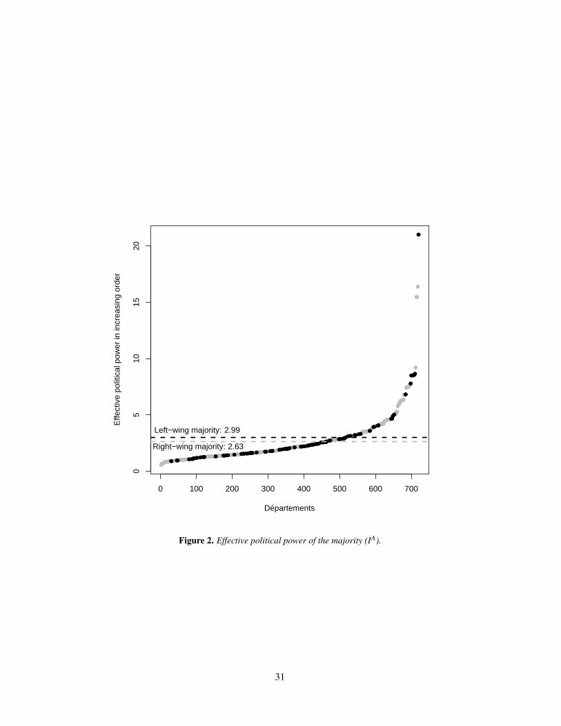
has no impact. To understand this result, we may have a look at Figures 2 to 5. They

depict respectively the effective political power index, the electoral margin and the Herfindahl-

Hirschman Index of the majority, and the Herfindahl-Hirschman Index of the opposition for

the 90 départements over the eight years of our study. As depicted by Figure 2, the average

effective political power indexes of the left-wing (in black on the figure) and right-wing

majorities (in grey on the figure), IA, are pretty close, reaching respectively 2.99 and 2.63.

However the average electoral margin of the right-wing départements is much higher than

that of the left-wing départements, respectively 3.6 and 2.54 (see Figure 3) and the left-wing

coalitions are more concentrated than the right-wing coalitions, whatever their status, majority

or opposition (see Figure 4 and 5). Hence, it seems that the opposition’s fragmentation might

play a role only in the case of a relatively small electoral margin of the majority. Having a

large electoral margin on average, the right-wing départements tend to be more fragmented

but the concentration of the left-wing opposition does not matter in such cases.

More generally, according to Figures 2 to 5, it looks like there may be a kind of

substituability between electoral margin and fragmentation. The larger the electoral margin

of the majority, the more fragmented it is. Politicians would derive utility from leading

their own party but they also know that fragmentation affects the effective political power

19

of their coalition. As a result there could be a trade-off between fragmentation and the

effective political power of a coalition, the nature of this trade-off being conditioned by the

fragmentation of the opposition coalition.

To conclude, our model begins to analyze the relationship between parties, coalitions,

and fragmentation, though it also raises many questions. Is there some kind of competition

in concentration among competitive coalitions? Does the fragmentation of the majority

and the opposition have an impact on the volatility of expenditures (Crain 2003)? Does

fragmentation consequently lead to inefficient public spending? These and other questions

provide a formidable agenda for future research.

6. Acknowledgments

The authors would like to thank Arthur Charpentier, Fabio Padovano, Jean-Michel

Josselin, Antti Moisio, Christophe Tavéra, Sylvain Chabe-Ferret, Geneviève Tellier and two

anonymous referees of this journal for their helpful comments. We are also grateful to William

F. Shughart II for suggestions. Earlier versions of this paper were presented at the conference

of the ASRDLF (Clermond-Ferrand, 2009), the University of Eastern Piedmont (Alessandria,

2009), the annual JMA meeting (La Réunion, 2008), the annual meeting of the Public Choice

Society (San Antonio, 2008) and the PEARLE seminar (Tampere, 2007).

20

Notes

1Primo and Snyder (2008) show that this result might be reversed under certain conditions.We do not discuss this theory in our paper.

2For instance Rogers (2002) applies this theory to the production of legislation in theAmerican states.

3It should be stressed that the Random effects estimator also permits estimation ofcoefficients of time-invariant regressors, but this estimator is inconsistent if the fixed effectsmodel is the correct model (see for instance Cameron and Trivedi, 2005). In order to checkwhether random effects regressions were more appropriate, the specification test devised byHausman (1978) was also applied on equation (14). The Hausman statistic was equal to 57.07with a high level of significance. We consequently have no reason to believe that randomeffects regressions would be better than fixed effects regressions. Moreover, to be able to usethe Random effects estimator, Hausman and Taylor (1981) propose the use of instrumentsfor the variables that are likely to be correlated with the random effects. Unfortunately, thiscorrelation is unobservable and it is difficult to correctly specify the Hausman-Taylor model(Plümper and Troeger, 2007).

21

References

Alchian, A. A. and Demsetz, H. (1972). Production, information costs, and economicorganization. American Economic Review, 62:777–795.

Ashworth, J. and Heyndels, B. (2005). Government fragmentation and budgetary policy in’good’ and ’bad’ times in flemish municipalities. Economics and Politics, 17:245–263.

Beck, N. (2001). Time-series-cross-section data: What have we learned in the past few years?Annual Review of Political Science, 4:271–293.

Borge, L. E. and Rattsø, J. (2002). Spending growth with vertical fiscal imbalance:Decentralized government spending in Norway, 1880-1990. Economics and Politics,14:351–373.

Boyne, G. A. (1996). Constraints, choices and public policies. Greenwich, CT.: JAI Press.

Bradbury, J. C. and Crain, W. M. (2001). Legislative organization and government spending:cross-country evidence. Journal of Public Economics, 82:309–325.

Breunig, R. and Rocaboy, Y. (2008). Per-capita public expenditures and population size: anon-parametric analysis using french data. Public Choice, 136:429–445.

Buchanan, J. M. and Tullock, G. (1962). The calculus of consent: Logical foundations ofConstitutional Democracy. Ann Arbor, University of Michigan Press.

Cameron, A. and Trivedi, P. (2005). Microeconometrics: Methods and Applications.Cambridge U. Press.

Crain, W. (2003). Volatile states: Institutions, policy, and the performance of American stateeconomies. Ann Arbor: University of Michigan Press.

Crain, W. M. and Tollison, R. D. (1982). Team production in political majorities.Micropolitics, 2:111–121.

Gilligan, T. W. and Matsusaka, J. G. (1995). Deviations from constituent interests: The roleof legislative structure and political parties in the States. Economic Inquiry, 33:383–401.

Goldfeld, S. and Quandt, R. (1973). The estimation of structural shifts by switchingregressions. Annals of Economic and Social Measurement, 2:475–485.

Hausman, J. (1978). Specification tests in econometrics. Econometrica, 46:1251–1271.

Hausman, J. and Taylor, W. (1981). Panel data and unobservable individual effects.Econometrica, 49:1377–1398.

Kuster, S. and Botero, F. (2008). How many is too many? assessment of party systemfragmentation measurements with data from latin america. Prepared for the 2008 APSAAnnual Meeting.

22

Olson, M. (1965). The Logic of Collective Action. Cambridge, harvard university pressedition.

Padovano, F. and Venturi, L. (2001). Wars of attrition in Italian government coalitions andfiscal performance: 1984-1994. Public Choice, 109:15–54.

Perotti, R. and Kontopoulos, Y. (2002). Fragmented fiscal policy. Journal of PublicEconomics, 86:191–222.

Persson, T. and Tabellini, G. (2003). The economic effects of constitutions. MIT Press,Cambridge, MA.

Plümper, T. and Troeger, V. E. (2007). Efficient estimation of time-invariant and rarelychanging variables in finite sample panel analyses with unit fixed effects. Political Analysis,15:124–139.

Pommerehne, W. (1978). Institutional approaches to estimating public expenditures:Empirical evidence from Swiss municipalities. Journal of Public Economics, 9:255–280.

Poterba, J. M. (1994). State responses to fiscal crises: The effects of budgetary institutionsand politics. Journal of Political Economy, 102:799–821.

Primo, D. M. and Snyder, J. (2008). Distributive politics and the law of 1/n. The Journal ofPolitics, 70:477–486.

Rattsø, J. and Tovmo, P. (2002). Fiscal discipline and asymmetric adjustment of revenues andexpenditures: Local government responses to shocks in denmark. Public Finance Review,30:208–234.

Rogers, J. R. (2002). Free-riding in state legislatures. Public Choice, 113:59–76.

Roubini, N. and Sachs, J. D. (1989). Government spending and budget deficits in the industrialcountries. Economic Policy, 8:99–132.

Skaperdas, S. (1996). Contest success functions. Economic Theory, 7:283–290.

Tullock, G. (1980). Efficient rent seeking. In Buchanan, J., Tollisson, R., and Tullock, G.,editors, Toward a theory of rent seeking society, pages 97–112. College Station: TX, A&MUniversity Press.

Velasco, A. (2000). Debts and deficits with fragmented fiscal policy making. Journal ofPublic Economics, 76:105–125.

Volkerink, B. and de Haan, J. (2001). Fragmented government effects on fiscal policy: newevidence. Public Choice, 109:221–242.

Weingast, B., Shepsle, K. A., and Johnsen, C. (1981). The political ecomomy of benefitsand costs: A neoclassical approach to distributive politics. Journal of Political Economy,89:642–664.

23

Table 1. Serial correlation and cross-sectional dependence tests.

Estimator Test for serial correlation Test for cross-sectional dependencePooled-OLS 435.6963*** 48.4422***Geographical dummies 435.2672*** 48.2871***Plümper and Troeger procedure 143.4256*** 29.0321****** indicates significance at the 0.1% level.

Table 2. Geographical dummies.

Area RegionsWest Bretagne, Basse-Normandie, Pays de la Loire, Poitou-Charentes.North Nord-Pas-de-Calais, Haute Normandie, Picardie, Ile-de-France, Picardie.East Champagne-Ardenne, Lorraine, Franche-Comté.Centre Centre, Bourgogne, Auvergne.South-West Limousin, Aquitaine, Midi-Pyrénées.South-East Rhône-Alpes, Provence-Alpes-Côte d’Azur, Languedoc-Roussillon.

2.

24

Tabl

e3.

Polit

ical

Part

ies

atth

edé

part

emen

tLev

el.

Nam

eA

cron

ymE

nglis

hna

me

Polit

ical

ideo

logy

Rem

arks

1992

a19

94a

1998

a

Left-

win

gpo

litic

alpa

rtie

sC

onve

ntio

npo

urun

eA

ltern

ativ

ePr

ogre

ssis

teC

AP

Con

vent

ion

fora

Prog

ress

ive

Alte

rnat

ive

Farl

eft-

win

g,E

nvir

onm

enta

lism

Foun

ded

in19

94m

ainl

yby

form

erm

embe

rsof

the

PCF,

the

AD

S,th

ePS

and

The

Gre

ens.

Dis

solv

edin

1998

0%0%

0.38

%

Part

iCom

mun

iste

Fran

çais

PCF

Fren

chC

omm

unis

tPa

rty

Farl

eft-

win

g,L

eft-

win

g,C

omm

unis

mM

ajor

votin

gbl

ock.

Foun

ded

in19

206.

90%

6.47

%7.

31%

Alte

rnat

ive,

Dém

ocra

tie,

Soci

alis

me

AD

SA

ltern

ativ

e,D

emoc

racy

,So

cial

ism

Lef

t,Fa

rLef

t-W

ing,

Alli

ance

son

the

left

,Com

mun

ism

Foun

ded

in19

94m

ainl

yby

past

mem

bers

ofth

ePC

F0.

33%

0.36

%0%

Mou

vem

entd

esC

itoye

ns,

Mou

vem

entR

épub

licai

net

Cito

yen

MD

C,

MR

CC

itize

ns’M

ovem

ent,

Rep

ublic

anan

dC

itize

nM

ovem

ent

Lef

t-w

ing,

Soci

alde

moc

racy

,D

emoc

ratic

soci

alis

mFo

unde

dby

Jean

-Pie

rre

Che

vène

men

tin

1993

0%0.

25%

0.49

%

Ass

ocia

tion

pour

laD

émoc

ratie

etle

Dév

elop

pem

ent

AD

DA

ssoc

iatio

nfo

rD

emoc

racy

and

Dev

elop

men

t

Lef

t-w

ing,

Def

ense

ofde

moc

racy

and

hum

anri

ghts

,Hum

anita

rian

assi

stan

ce

Foun

ded

byH

assa

nM

okbe

lin

1991

,it

has

mer

ged

asa

resu

ltof

stud

ent

mov

emen

ts

0.03

%0.

05%

0.05

%

Gén

érat

ion

Éco

logi

eG

EE

colo

gyG

ener

atio

nL

eft-

Win

g,C

ross

-par

tyal

lianc

esof

gree

n-m

inde

dpo

litic

ians

Foun

ded

byB

rice

Lal

onde

in19

900.

19%

0.16

%0.

03%

Maj

orité

plur

ielle

Plur

alM

ajor

ityA

llian

ces

betw

een

the

MR

C,t

hePS

,th

ePC

F,th

ePR

G,a

ndT

heG

reen

sFo

unde

din

1997

0.19

%0%

0%

Les

Ver

tsT

heG

reen

sL

eft-

win

g,E

nvir

onm

enta

lism

Foun

ded

in19

820.

02%

0.05

%0.

14%

Part

isoc

ialis

tePS

Soci

alis

tPar

tyL

eft-

win

g,C

ente

rlef

t,So

cial

dem

ocra

cy,D

emoc

ratic

soci

alis

mM

ajor

votin

gbl

ock.

Rep

lace

dth

eSF

IOin

1969

23.8

9%22

.44%

30.2

8%

Part

irad

ical

dega

uche

,M

ouve

men

tdes

Rad

icau

xde

Gau

che

PRG

,M

RG

Lef

tRad

ical

Part

y,L

eft

Rad

ical

Mov

emen

tC

ente

rlef

t,So

cial

dem

ocra

cy,

Dem

ocra

ticso

cial

ism

Foun

ded

in19

71.

Hei

rof

the

Part

iré

publ

icai

n,ra

dica

let

radi

cal-

soci

alis

te

1.83

%1.

59%

1.70

%

Mou

vem

entÉ

colo

gist

eIn

dépe

ndan

tM

EI

Inde

pend

entE

colo

gica

lM

ovem

ent

Cen

ter,

Cen

terL

eft,

Env

iron

men

talis

mFo

unde

dby

Ant

oine

Wae

chte

rin

1994

0%0%

0.03

%

Rig

ht-w

ing

polit

ical

part

ies

Mou

vem

entD

esR

efor

mat

eurs

MD

RR

efor

mis

tsM

ovem

ent

Cen

ter,

Cen

terr

ight

,Am

bigu

ous

Foun

ded

byJe

an-P

ierr

eSo

isso

nin

1992

0.27

%0.

08%

0%

Uni

onD

émoc

ratiq

ueIn

tern

atio

nale

UD

IIn

tern

atio

nalD

emoc

rat

Uni

onC

ente

r,C

ente

rrig

ht,C

onse

rvat

ism

,C

hris

tian

dem

ocra

cy,L

iber

alis

mIn

tern

atio

nal

ogan

izat

ion

foun

ded

in19

830%

0.03

%0%

Uni

onpo

urla

Dém

ocra

tieFr

ança

ise

UD

FU

nion

forF

renc

hD

emoc

racy

Cen

terr

ight

,Chr

istia

nde

moc

racy

min

ority

fact

ions

,Soc

iall

iber

alis

mM

ajor

votin

gbl

ock.

Foun

ded

byV

alér

yG

isca

rdd’

Est

aing

in19

7825

.45%

25.1

6%18

.91%

Ras

sem

blem

entp

ourl

aR

épub

lique

RPR

Ral

lyfo

rthe

Rep

ublic

Rig

ht-w

ing,

Con

serv

atis

m,G

aulli

smM

ajor

votin

gbl

ock.

Foun

ded

byJa

cque

sC

hira

cin

1976

22.1

1%22

.39%

17.9

9%

Cen

tre

Nat

iona

ldes

Indé

pend

ants

etPa

ysan

sC

NI,

CN

IPN

atio

nalC

ente

rof

Inde

pend

ents

and

Peas

ants

Alli

ance

sm

ainl

ybe

twee

nth

eU

DF,

the

RPR

,the

MPF

,and

the

FNFo

unde

dby

Rog

erD

uche

tinin

1948

asth

eN

atio

nalC

entr

eof

Inde

pend

ents

0.57

%0.

33%

0.11

%

Mou

vem

entp

ourl

aFr

ance

MPF

Mov

emen

tfor

Fran

ceR

ight

-win

g,Fa

rrig

ht-w

ing

Foun

ded

byPh

ilipp

ede

Vill

iers

in19

940%

0%0.

14%

Fron

tNat

iona

lFN

Nat

iona

lFro

ntFa

rrig

ht-w

ing,

Nat

iona

lism

Foun

ded

byJe

an-M

arie

Le

Pen

in19

720.

08%

0.11

%0.

19%

aSh

are

ofse

ats

held

inth

e90

cons

ider

eddé

part

emen

tsfo

rthe

1992

,199

4an

d19

98ca

nton

alel

ectio

ns.I

tsho

uld

best

ress

edth

atso

me

ofth

eca

ndid

ates

wer

ein

depe

nden

t,i.e

.did

notb

elon

gto

apo

litic

alpa

rty.

Thi

sis

why

the

sum

ofth

est

atis

tics

isno

tota

llyeq

ualt

o10

0%.A

sre

gard

sth

ees

timat

ions

ofSe

ctio

n4,

we

knew

the

ideo

logy

ofth

ese

inde

pend

entc

andi

date

s,i.e

.,Fa

rle

ft-w

ing,

Lef

t-w

ing

orR

ight

-win

g.To

com

pute

the

Her

finda

hl-H

irsc

hman

Inde

xes,

we

did

asif

thes

eca

ndid

ates

belo

nged

toth

esa

me

polit

ical

part

y,i.e

."Fa

rlef

tind

epen

dent

cand

idat

es",

"Lef

t-w

ing

inde

pend

entc

andi

date

s"an

d"R

ight

-win

gin

depe

nden

tcan

dida

tes"

.

25

Table 4. Summary Statistics.a

Variables Mean Min Max SD

SOCIAL 1370 646 2467 283TAX 0.521 0.067 0.884 0.076INCOME 42353 29460 80474 6332GRANT S 914 383 2991 308POP 585984 72390 2555471 435502OLD 0.2219 0.1231 0.3362 0.0430DENS 320 14 8113 1140LEFT 0.261 0 1 0.440IA 2.722 0.5689 21 2.287

a Number of observations: 720. SOCIAL, GRANT S andINCOME are in current Francs.

Table 5. Description of the Variables.

Variable ContentSOCIAL Per capita social expenditures. Source: Direction Genérale des collectivités locales

(DGCL).TAX Household tax share, which is defined as the household share (tax on housing and property

taxes) of département taxes (property taxes, local business tax, tax on housing). Source:Direction Genérale des collectivités locales (DGCL).

INCOME Mean household taxable income. Source: Direction Genérale des collectivités locales(DGCL).

GRANT S Grants received by the département (mainly from the central government) per inhabitant.Source: Direction Genérale des collectivités locales (DGCL).

POP Local population. Source: Institut National des la Statistique et des Etudes economiques(INSEE).

OLD Share of population beeing more than 60. Source: Direction Genérale des collectivitéslocales (DGCL).

DENS Population density of the département. Source: Direction Genérale des collectivitéslocales (DGCL).

T REND Trend. It takes the value 0 for year 1992, 1 for year 1993, ...LEFT Ideology of the majority coalition. It is a dummy equal to one if the majority coalition

in the département council is on the left and zero if on the right. Source: Newspaper LeMonde.

IR = sR

sL

√HR

HL Right-wing coalition effective political power index:sR: Number of seats held by the right-wing coalition. Source: Newspaper Le Monde.sL: Number of seats held by the Left-wing coalition. Source: Newspaper Le Monde.HR = ∑

nR

p=1(αR

p)2:Herfindahl-Hirschman Index of the right-wing coalition where nR is

the number of right-wing parties and αRp is the share of seats of party p in the right wing

group.HL = ∑

nL

p=1(αL

p)2:Herfindahl-Hirschman Index of the left-wing coalition.

IL = sL

sR

√HL

HR Left-wing coalition effective political power index.

26

Table 6. Estimation results (Pooled-OLS with panel robust standard errors).a

Specification 1: Specification 2: Specification 3: Specification 4: Specification 5:All the Left-wing Right-wing Left-wing Right-wing

départements départements départements départements départements

Intercept -9.203*** -8.663*** -9.199*** -7.862*** -9.728***(-17.900) (-8.8255) (-12.194) (-8.886) (-12.626)

Taxe share: ln(TAXi,t) -0.086** -0.119 -0.087 . -0.118 . -0.110*(-2.615) (-1.593) (-1.660) (-1.956) (-2.098)

Income: ln(yi,t) 0.453*** 0.287** 0.470*** 0.240** 0.513***(8.206) (3.043) (6.104) (2.606) (6.612)

Grants: ln(si,t) 0.446*** 0.354*** 0.466*** 0.359*** 0.468***(20.329) (7.964) (17.730) (7.768) (17.533)

Population: ln(Ni,t) 0.029** 0.040* 0.028* 0.008 0.027.

(2.773) (2.148) (2.077) (0.551) (1.944)Share of elderly: OLDi,t 0.660*** 1.904*** 0.467* 1.792*** 0.569**

(3.659) (3.453) (2.292) (3.508) (2.638)Population density: ln(DENSi,t) 0.063*** 0.090*** 0.062*** 0.102*** 0.061***

(8.880) (7.697) (5.748) (8.165) (5.490)Trend: T RENDt 0.012*** 0.013** 0.012*** 0.021*** 0.012***

(4.247) (2.819) (3.460) (4.399) (3.469)

Left-wing effective political power: ln(ILi,t) 0.047*** 0.035*

(4.326) (2.328)Right-wing effective political power: ln(IR

i,t) -0.029*** -0.026**(-3.451) (-2.823)

Electoral margin of coalition A: ln((sA/sB)i,t) 0.044** -0.027**(2.740) (-2.849)

Herfindahl-Hirschman Index of coalition A: ln(HAi,t) 0.142* -0.144**

(2.314) (-3.120)Herfindahl-Hirschman Index of coaltion B: ln(HB

i,t) -0.274*** -0.033(-4.775) (-0.963)

Adjusted R2 0.6067 0.6354 0.5266 0.6645 0.5316Number of observations 720 188 532 188 532

a t value in parentheses.*** , **, *, and . indicate significance at 0.1%,1%, 5% and 10% level, respectively.

27

Table 7. Estimation results (Geographical dummies with panel robust standard errors).a



Taxe share: ln(TAXi,t) -0.081* -0.044 -0.137* -0.062 -0.158**(-2.407) (-1.338) (-2.488) (-1.568) (-2.870)

Income: ln(yi,t) 0.397*** 0.137 0.516*** 0.120 0.563***(5.960) (1.438) (5.076) (1.147) (5.350)

Grants: ln(si,t) 0.431*** 0.321*** 0.462*** 0.329*** 0.467***(19.365) (7.499) (17.874) (7.682) (17.916)

Population: ln(Ni,t) 0.017 -0.017 0.018 -0.023 0.011(1.613) (-0.773) (1.203) (-1.055) (0.742)

Share of elderly: OLDi,t 0.505* 0.535 0.686* 1.108 . 0.604 .

(2.043) (0.883) (2.114) (1.738) (1.915)Population density: ln(DENSi,t) 0.060*** 0.093*** 0.052*** 0.111*** 0.054***

(7.818) (6.605) (3.815) (6.889) (3.918)Trend: T RENDt 0.014*** 0.022*** 0.010* 0.027*** 0.010*

(4.686) (6.172) (2.390) (7.688) (2.474)

Left-wing effective political power: ln(ILi,t) 0.043*** 0.007


i,t) -0.025* -0.025*(-2.543) (-2.297)

Electoral margin of the majority: ln((SA/SB)i,t) 0.0190 -0.026*(0.982) (-2.324)

Herfindahl-Hirschman Index of the majority: ln(HAi,t) 0.156*** -0.169***

(2.674) (-3.830)Herfindahl–Hirschman Index of the opposition: ln(HB

i,t) -0.239*** -0.043(-3.614) (-1.137)



28

Table 8. Estimation results (Plümper and Troeger procedure with panel robust standard errors).a



Intercept -6.351*** -8.116*** -4.395*** -8.470*** -4.483***(-26.904) (-15.231) (-14.981) (-18.428) (-15.866)

Taxe share: ln(TAXi,t) -0.083** -0.116 -0.132*** -0.010 -0.115***(-6.975) (-0.893) (-9.912) (-0.507) (-8.611)

Income: ln(yi,t) 0.154*** 0.364*** 0.002 0.393*** 0.009(6.951) (7.112) (0.109) (7.895) (0.349)

Grants: ln(si,t) 0.410*** 0.472*** 0.434*** 0.436*** 0.402***(54.139) (26.209) (56.200) (19.978) (51.858)

Population: ln(Ni,t) 0.025** 0.030** 0.002 0.002 -0.013*(4.572) (3.066) (0.421) (0.287) (-2.552)

Share of elderly: OLDi,t 0.735*** 0.835*** 0.483*** 1.007*** 0.411***(10.723) (3.921) (6.929) (4.964) (6.389)

Population density: ln(DENSi,t) 0.085*** 0.072*** 0.118*** 0.085*** 0.119***(22.992) (11.579) (26.642) (13.704) (26.393)

Trend: T RENDt 0.014*** 0.012*** 0.016*** 0.016*** 0.015***(12.012) (4.858) (13.251) (7.522) (12.482)

Left-wing effective political power: ln(ILi,t) 0.042*** 0.031***


i,t) -0.029*** -0.029***(-8.670) (-9.418)

Electoral margin of the majority: ln((SA/SB)i,t) 0.034*** -0.025***(4.931) (-7.537)

Herfindahl-Hirschman Index of the majority: ln(HAi,t) 0.184*** -0.079***

(6.379) (-4.049)Herfindahl-Hirschman Index of the opposition: ln(HB

i,t) -0.245*** -0.005(-8.963) (-0.409)



The following variables were considered as time-invariant or rarely changing variables : POP, OLD, DENS, IA, sA, HA and HB.

29

0 100 200 300 400 500 600 700

1000

1500

2000

2500

Départements

Per

cap

ita e

xpen

ditu

res

in in

crea

sing

ord

er

Left−wing:

Right−wing:

1542.73

1309.53

Figure 1. Per capita social expenditures in Francs (SOCIAL).

30

0 100 200 300 400 500 600 700

05

1015

20

Départements

Effe

ctiv

e po

litic

al p

ower

in in

crea

sing

ord

er

Left−wing majority:

Right−wing majority:

2.99

2.63

Figure 2. Effective political power of the majority (IA).

31

0 100 200 300 400 500 600 700

05

1015

2025

30

Départements

Ele

ctor

al m

argi

n in

incr

easi

ng o

rder



2.54

3.6

Figure 3. Electoral margin of the majority (sA/sB).

32

0 100 200 300 400 500 600 700

0.2

0.4

0.6

0.8

1.0

Départements

Her

findh

al in

dex

in in

crea

sing

ord

er



0.597

0.328

Figure 4. Herfindhal-Hirschman index of the majority (HA).

33

0 100 200 300 400 500 600 700

0.2

0.4

0.6

0.8

1.0

Départements

Her

findh

al in

dex

in in

crea

sing

ord

er

Right−wing opposition:

Left−wing opposition:

0.414

0.573

Figure 5. Herfindhal-Hirschman index of the opposition (HB).

34

political fragmentation, party ideology and public...

Documents