playing hard or soft? : a simulation of indonesian ... filecharles joseph, janu dewandaru, iman...

1

PLAYING HARD OR SOFT? : A SIMULATION OF INDONESIAN MONETARY POLICY IN TARGETING LOW INFLATION USING A DYNAMIC GENERAL EQUILIBRIUM MODEL Charles JOSEPH, Janu DEWANDARU, Iman GUNADI In the real world, the most “optimal” policy rule is not always the most “desirable” rule. There are always preferences, considerations and judgements involved during the process of monetary policy formulation. The hawks will always prefer a stronger stance and want to play as hard as possible in fighting the evil of inflation, while the doves prefer a softer, moderate stance. This paper attempts to simulate how such preferences affect the dynamics of the Indonesian economy using GEMBI, a stochastic non-linear dynamic GE model developed by Bank Indonesia. Preferences between playing hard by the hawks and playing soft by the doves in attaining the pre-announced 6%-7% targeted inflation are distinguished. The hawks will use a policy rule that achieves the target as soon as possible. The doves will use a policy rule which is more “accommodating” to the economy, and hence they are willing to live with a slightly higher inflation rate than the pre-announced target or to achieve the target over a longer time horizon.

2

1. Introduction

Over the past decade inflation targeting (IT) has become a fashionable

framework for monetary policy in many countries. Inflation targeting is a framework

of monetary policy marked by a pre-announced official inflation target at a certain

period of time. The announcement is intended to assure the public that the long-term

objective of monetary policy is to achieve stable and low inflation. Two important

elements of inflation targeting are the target itself and the commitment of the

government to the objective of monetary policy, which is low inflation. In preparing

for the implementation of an inflation targeting (IT) framework, Bank Indonesia has

been exploring the concept of inflation targeting itself and the operational framework

on how to implement the central bank reaction function using a Taylor rule in

achieving the targeted inflation in short medium and long term contexts. To this end, a

number of macroeconomic models have been developed to support the

implementation of the inflation targeting framework. One of the existing models is the

General Equilibrium Model of Bank Indonesia (hereafter called GEMBI)1.

General Equilibrium models are needed for medium and longer-term policy

analysis and for evaluation of related policy issues. The policy evaluation issues

include choosing an optimal policy rule in reaching a targeted inflation rate set by the

central bank for a particular period of time, both in short-medium and longer term

contexts. To this end, there are pitfalls, which can pose serious dangers to economic

growth or longer-term stability. The proper design and policy implementation requires

a careful analysis of the broader macroeconomic “environment” in which these policy

options would be undertaken.

While the short-term impact of policy options is well captured by the short-

term econometric oriented models such as MODBI (Annual Model of Bank

Indonesia) and the quarterly model such as SOFIE (Short Term and Forecasting

Model of the Indonesian Economy), GEMBI plays a role in complementing these

models as a flight simulator in predicting the dynamics of interest rate policy options

aimed at achieving the targeted inflation rate set by policy makers.

1 GEMBI is a stochastic non-linear dynamic general equilibrium (SNDGE) model. The construction of the model started in June 2000, developed by a team of Bank Indonesia economists at the Macroeconomic Studies Division of the Research and Monetary Policy Directorate (DKM/SEM) of Bank Indonesia. The model evolved from a theoretical concept to an operational policy instrument, for ongoing analysis and evaluation, with the assistance and advice of Prof. Paul D McNelis under the

3

This paper attempts to explore the interest rate policy options available to

policy makers in reaching a targeted inflation rate within a certain period of time

using the Taylor rule approach. In the real world the most “optimal” policy rule is

not always the most “desirable” rule. There are always preferences, considerations

and judgements involved during the process of monetary policy formulation. Inflation

hawks will always prefer a stronger stance and want to play as hard as possible in

fighting the evil of inflation, while doves prefer a softer, moderate stance. This paper

tries to simulate how hawks or doves preferences affect the long-run dynamics of the

Indonesian economy using GEMBI. Preferences between playing hard by the hawks

and playing soft by the doves in attaining the pre-announced 6% - 7% inflation target

are used in this simulation process. The hawks will adopt a policy rule to reach the

target as soon as possible. The doves adopt a policy rule which is more

“accommodating” to the economy, and hence they are willing to live with a slightly

higher inflation rate than the pre-announced target or to attain the target rate over a

longer time horizon.

The next sections include the structure of GEMBI, the result of the alternative

policy simulations and the conclusion.

2. Structure of GEMBI

GEMBI has been developed for almost two years from a very simple model to

a more complex one. At this phase, important sectors of the economy have been

incorporated into the model. There are five sectors in the model: households, banks,

firms produces traded and non-traded goods, the external sector, and the government.

All agents except government have their own objective function and budget

constraint. Optimization from each agent results in the formulation that will play its

role in the model. The explanation of each agent is described as follows:

2.1. Households

The objective of households is to maximize the utility of household

consumption.

Partnership for Economic Growth (PEG) project of the U.S. Agency for International Development (USAID).

4

Max [ ]∑ ∑ ++

++ = it

itit

it ccU log)( ββ ρ

β+

=1

1

where:

c = consumption; ρ = social discount rate; η = coefficient of relative risk aversion.

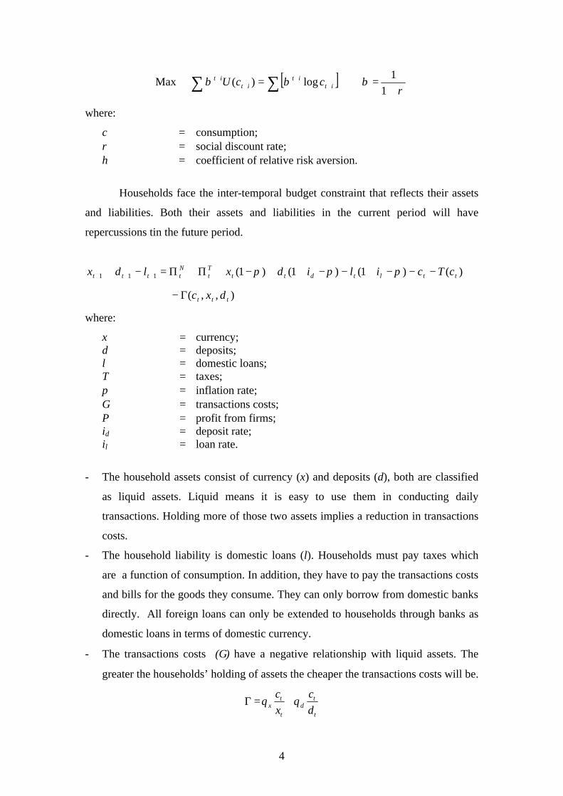
Households face the inter-temporal budget constraint that reflects their assets

and liabilities. Both their assets and liabilities in the current period will have

repercussions tin the future period.

)()1()1()1(111 ttltdttTt

Ntttt cTcilidxldx −−−+−−++−+Π+Π=−+ +++ πππ

),,( ttt dxcΓ−

where:

x = currency; d = deposits; l = domestic loans; T = taxes; π = inflation rate; Γ = transactions costs; Π = profit from firms; id = deposit rate; il = loan rate.

- The household assets consist of currency (x) and deposits (d), both are classified

as liquid assets. Liquid means it is easy to use them in conducting daily

transactions. Holding more of those two assets implies a reduction in transactions

costs.

- The household liability is domestic loans (l). Households must pay taxes which

are a function of consumption. In addition, they have to pay the transactions costs

and bills for the goods they consume. They can only borrow from domestic banks

directly. All foreign loans can only be extended to households through banks as

domestic loans in terms of domestic currency.

- The transactions costs (Γ) have a negative relationship with liquid assets. The

greater the households’ holding of assets the cheaper the transactions costs will be.

t

td

t

tx d

cxc

θθ +=Γ

5

- Households do not only represent labor employed by firms, but also are the

owners. There is a transfer from firms to households in the form of wage

payments and dividends (traded: TΠ and non-traded firms: NΠ ). Initially, all the

receipts from firms to households will be used to pay households’ debts.

Additional income from firms will be held by households in the banks as deposits.

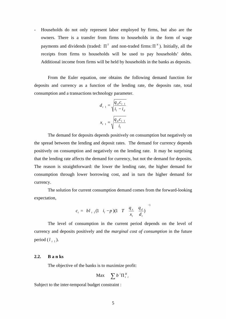
From the Euler equation, one obtains the following demand function for

deposits and currency as a function of the lending rate, the deposits rate, total

consumption and a transactions technology parameter.

dl

tdt ii

cd

−= +

+1

1

θ

l

tdt i

cx 1

1+

+ =θ

The demand for deposits depends positively on consumption but negatively on

the spread between the lending and deposit rates. The demand for currency depends

positively on consumption and negatively on the lending rate. It may be surprising

that the lending rate affects the demand for currency, but not the demand for deposits.

The reason is straightforward: the lower the lending rate, the higher demand for

consumption through lower borrowing cost, and in turn the higher demand for

currency.

The solution for current consumption demand comes from the forward-looking

expectation, 1

1 )1)(1(−

+

+++−+=

t

d

t

xltt dx

Ticθθ

πβλ

The level of consumption in the current period depends on the level of

currency and deposits positively and the marginal cost of consumption in the future

period ( 1+tλ ).

2.2. B a n ks

The objective of the banks is to maximize profit:

Max ∑ +Π Bit

iβ

Subject to the inter-temporal budget constraint :

6

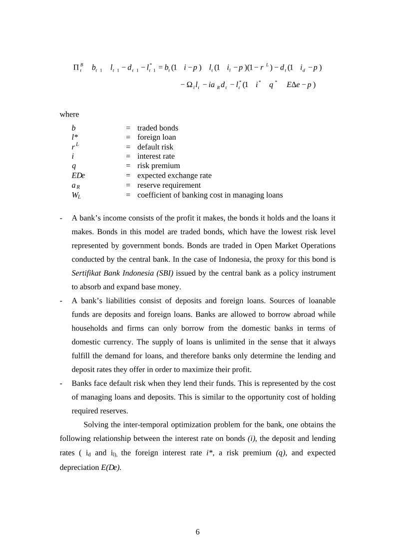
)1()1)(1()1(*1111 πρππ −+−−−++−+=−−++Π ++++ dt

Lltttttt

Bt idilibldlb

)1( *** πθα −∆+++−−Ω− eEildil ttRtl

where

b = traded bonds l* = foreign loan ρL = default risk i = interest rate θ = risk premium E∆e = expected exchange rate αR = reserve requirement ΩL = coefficient of banking cost in managing loans

- A bank’s income consists of the profit it makes, the bonds it holds and the loans it

makes. Bonds in this model are traded bonds, which have the lowest risk level

represented by government bonds. Bonds are traded in Open Market Operations

conducted by the central bank. In the case of Indonesia, the proxy for this bond is

Sertifikat Bank Indonesia (SBI) issued by the central bank as a policy instrument

to absorb and expand base money.

- A bank’s liabilities consist of deposits and foreign loans. Sources of loanable

funds are deposits and foreign loans. Banks are allowed to borrow abroad while

households and firms can only borrow from the domestic banks in terms of

domestic currency. The supply of loans is unlimited in the sense that it always

fulfill the demand for loans, and therefore banks only determine the lending and

deposit rates they offer in order to maximize their profit.

- Banks face default risk when they lend their funds. This is represented by the cost

of managing loans and deposits. This is similar to the opportunity cost of holding

required reserves.

Solving the inter-temporal optimization problem for the bank, one obtains the

following relationship between the interest rate on bonds (i), the deposit and lending

rates ( id and il), the foreign interest rate i*, a risk premium (θ), and expected

depreciation E(∆e).

7

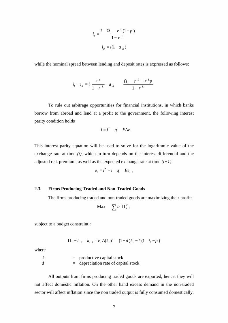
L

Ll

l

ii

ρπρ

−−+Ω+

=1

)1(

)1( Rd ii α−=

while the nominal spread between lending and deposit rates is expressed as follows:

−−+Ω

+

−

−=−

L

LLl

RL

L

dl iiiρ

πρρα

ρρ

11

To rule out arbitrage opportunities for financial institutions, in which banks

borrow from abroad and lend at a profit to the government, the following interest

parity condition holds

eEii ∆++= θ*

This interest parity equation will be used to solve for the logarithmic value of the

exchange rate at time (t), which in turn depends on the interest differential and the

adjusted risk premium, as well as the expected exchange rate at time (t+1)

1*

+++−= tt Eeiie θ

2.3. Firms Producing Traded and Non-Traded Goods

The firms producing traded and non-traded goods are maximizing their profit:

Max ∑ +Π Tit

iβ

subject to a budget constraint :

)1()1()(11 πδε α −+−−+=+−Π ++ lttttttt ilkkAkl

where

k = productive capital stock δ = depreciation rate of capital stock

All outputs from firms producing traded goods are exported, hence, they will

not affect domestic inflation. On the other hand excess demand in the non-traded

sector will affect inflation since the non traded output is fully consumed domestically.

8

However, imported goods affect inflation through their prices which are related to the

depreciation of the exchange rate. Some points need to be noted as follows:

- Output of the firms will be converted in the form of wage payments and will be

used in investment spending and loan payments. If there is additional surplus, it

will be transferred to households as dividends and will be deposited in the banking

system.

- The production technology is Cobb-Douglass with capital as the factor of

production. αε )( Tt

TTt kAy = . For simplification, labor is not a constraint and is

always in equilibrium.

- Firms’ assets are in the form of capital and their production output while their

liabilities are in the form of domestic loans. The firm cannot borrow from the

foreign market directly, but is allowed to borrow from domestic banks in terms of

domestic currency.

- Following Kydland and Prescott, it is also possible to introduce “time to build”

dynamics, in which new investment comes “on line” as productive capital, only

with a lag of one to several quarters. In this case, the actual productive capital

stock in each period is a function of lagged investment gradually coming “on

line”, less depreciation:

1,10

)1(ˆ*

011

=≤≤

−+=

∑

∑=

−−

ii

T

i

jtj

Kti

jt

xx

kIxk j δ

where x is the proportion of the desired capital stock which comes on line at

period i = 0 and T* represents the time horizon for the total investment plan to

be realized.

- Other than depreciation of capital, firms also face adjustment costs that make it

costly to convert capital already included in the production process (‘putty-clay”).

Production itself is influenced by two types of shocks, i.e., terms of trade shocks

and non-traded production shocks.

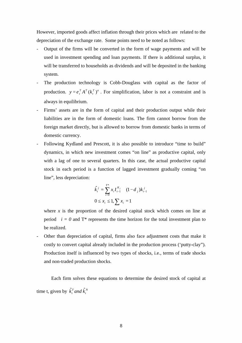
Each firm solves these equations to determine the desired stock of capital at

time t, given by Nt

Tt kandk ˆˆ

9

11

1ˆ

−

+

+−=

α

αεδπ

TTt

lTt A

ik

11

1ˆ

−

+

+−=

α

αεδπ

NNt

lNt A

ik

2.4. Government

The government issues bonds to finance budget deficits. It spends money on

non-traded goods, gN; pays back its previous debts and collects seigniorage revenue

on holdings of base money, m0:

)()()/( ,01 tttNT

tt cTmbizggbb −−−++=−+ ππ

where

b = stock of domestic bonds held by government; gN = government expenditure on non-traded goods; πm = inflation tax/seigniorage.

It is assumed that the government bonds are held by banks. If government

borrowing relative to GDP is above a critical threshold, the government will raise

taxes in order to balance the budget and to freeze the expansion of government debt.

Similarly, if the government is running a surplus, it will reduce its debt until the debt

is retired. Then the government will reduce taxes levied on the households in a lump-

sum fashion.

2.5. Parameterized Expectations

The above model is constructed for simulation and policy evaluation through

numerical approximation algorithms. One could simulate the model to obtain the

dynamics of the endogenous variables, given the exogenous policy rules, the shocks

and the specification of the underlying parameters and initial conditions. The main

issue for simulating this model is that there are forward looking variables for

consumption and the exchange rate: 1

1 )1)(1(−

+

+++−+=

t

d

t

xltt dx

Ticθθ

πβλ

10

1*

+++−= tt Eeiie θ

How to find values at time t as a function of variables expected at time t+1 is

the central issue for “solving” such “a forward looking” stochastic non-linear dynamic

general equilibrium model.

Following Marcet (1988, 1993), Den Haan and Marcet (1990, 1994), and

Duffy and McNelis (2000), the approach of this study is to “parameterize” the

forward looking expectations in this model, with non-linear functional forms ψE, ψC:

[ ] );()('1 11 λψγλ Ω=Γ++⋅ −+ tc

ctttt xcRE

);( 11 EtE

tt xeE Ω= −+ ψ

where R=(1+iL-π) and xt represents a vector of observable variables at time t, of

traded and non-traded production, the marginal utility of consumption, the real

interest rate, and the real exchange rate:

xt = yT, yN,λ,r,z

The functional form for ψE, ψC is usually a second order polynomial

expansion (see, for example, Den Haan and Marcet (1994)). However, Duffy and

McNelis (2001) have shown that the neural networks have produced results with

greater accuracy for the same number of parameters, or equal accuracy with few

parameters, than the second order polynomial approximation. Judd (1996) classifies

this approach as a “projection” or a “weighted residual” method for solving functional

equations, and notes that the approach was originally developed by Williams and

Wright (1982, 1984, 1991). These authors pointed out that the conditional expectation

of the future gain price as a “smooth function” of the current state of the market, and

that this conditional expectation can be used to characterize equilibrium.

The specification of the functional forms );( EtE x Ωψ and );( Ct

C x Ωψ

according to the neural network approximation is done in the following way:

∑=

=*

1,,

J

jtjjtk xbn

11

tintke

N,1

1, −+

=

∑=

=*

1,

K

ktkkt Nκψ

where J* is the number of exogenous or input variables, K* is the number of neurons,

nt is a linear combination of the input variables, Nt is a logsigmoid or logistic

transformation of nt, and ψt is the neural network prediction at time t of either (et+1)

or [ ] cttt cR Γ++⋅+ )('11 γλ .

As seen in this equation, the only difference from ordinary non-linear

estimation relating “regressors” to a “regressand” is the use of the hidden nodes or

neurons, N. One forms a neuron by taking a linear combination of the regressors and

then transforming this variable by the logistic or logsigmoid function. One then

proceeds to thus one or more of these neurons in a linear way to forecast the

dependent variable ψt.

Judd (1996) notes that the neural networks provide us with an “inherently non

linear functional form” for approximation, in contrast with methods based on linear

combinations of polynomial and trigonometric functions. Both Judd (1996) and

Sargent (1997) have drawn attention to the work of Barron (1993), who found that

neural networks do a better job of “approximating” any non linear function than

polynomials, in the sense that a neural network achieves the same degree of in sample

predictive accuracy with fewer parameters, or achieves greater accuracy, using the

same number of parameters. For this reason, Judd (1996) concedes that neural

networks may be particularly efficient at “multidimensional approximation”.

The main choices that one has to make for a neural network is J*, the number

of regression variables, and K*, the number of hidden neurons, for predicting a given

variable ψt. Generally, a neural network with only one hidden neuron closely

approximates a simple linear model, whereas larger numbers of neurons approximate

more complex non linear relationships. Obviously, with a large number of

“regressors” x and with a large number of neurons N, one approximates progressively

more complex non-linear phenomena, with an increasingly larger parameter set.

The “solution” for the parameters EEE b κ,=Ω and λλλ κ,b=Ω of the

neural network functional specification for ψE and ψλ is through recursive estimation.

12

Initially, the parameter sets ΩE and Ωλ are specified at random initial values. The full

model is then simulated for a long interval. Then the squared forecast errors for

ln(Et+1) and ln(λt+1Rt) are computed, based on the sum of the squared difference

realized values of ln(Et+1), λt+1 and the predictions given by ψE, ψλ based on the

initial values ΩE and Ωλ. These parameter sets are then updated in a recursive

estimation process, as the models are simulated repeatedly, until convergence is

achieved, when the sum of squared differences between the approximated and the

model generated values ψE, ψλ is minimized.

Judd (1998) calls this method a “fixed point iteration” with simulation and non

linear optimisation to compute the critical conditional expectation, in this case for Et+1

and λt+1. Judd (1998 : p 601) calls this use of simulation “intuitively natural” and

related to rational expectation “learning ideas”.

The idea behind this numerical approximation for solving for the “forward

expectation” for ln(Et+1) and (λt+1) is that agents do not know perfectly the underlying

model, but have to “learn it” from observations and minimizing forecast errors

through time. While this approach to the formulation of expectations seems to

contradict pure rationality of economic agents, Hansen and Sargent (2000) recently

noted that economists readily concede that all models are approximations, in order to

be tractable, i.e. both feasible to solve and to simulate. But they also note that with

tractability comes a form of misspecification, which is unavoidable in applied

economic research.

3. Inflation Targeting Using Soft or Hard Policy Rules

GEMBI is constructed with a Taylor rule reaction function where the central

bank controls the short-term interest rate as it responds to price conditions and the

output gap. Under this monetary framework, the central bank tries to achieve a

targeted inflation rate by adjusting the short-term interest rate through open market

operations. The appropriate interest rate is the rate which is consistent with a Taylor

Rule. In this model, the Taylor rule is a function of last period’s interest rate, the

deviation between expected inflation and targeted inflation, and the output gap.

13

− The Taylor rule as a reaction function will produce the path of the interest rate as

an intermediate target variable. Open market operations (Cut off Rate) are directed

to reach that path.

− The change in the stock of bonds will change the money supply in the economy.

The money supply is assumed to be equal to the demand for money since both are

affected by the interest rate generated by the Taylor rule.

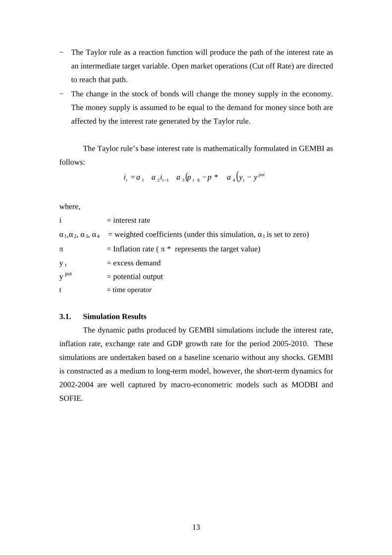
The Taylor rule’s base interest rate is mathematically formulated in GEMBI as

follows:

( ) ( )pottttt yyii −+−++= +− 463121 * αππααα

where,

i = interest rate

α1,α2, α3, α4 = weighted coefficients (under this simulation, α1 is set to zero)

π = Inflation rate ( π * represents the target value)

y t = excess demand

y pot = potential output

t = time operator

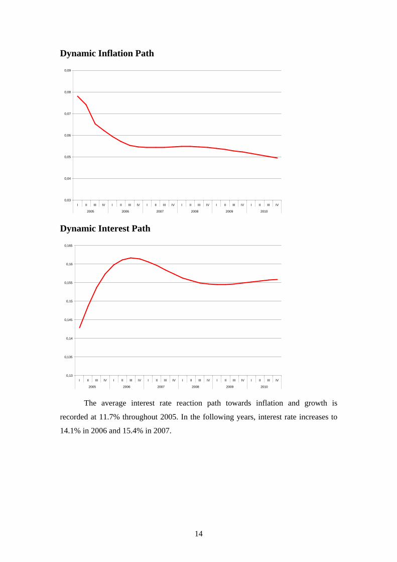
3.1. Simulation Results

The dynamic paths produced by GEMBI simulations include the interest rate,

inflation rate, exchange rate and GDP growth rate for the period 2005-2010. These

simulations are undertaken based on a baseline scenario without any shocks. GEMBI

is constructed as a medium to long-term model, however, the short-term dynamics for

2002-2004 are well captured by macro-econometric models such as MODBI and

SOFIE.

14

Dynamic Inflation Path

0,03

0,04

0,05

0,06

0,07

0,08

0,09

I II III IV I II III IV I II III IV I II III IV I II III IV I II III IV

2005 2006 2007 2008 2009 2010

Dynamic Interest Path

0,13

0,135

0,14

0,145

0,15

0,155

0,16

0,165


2005 2006 2007 2008 2009 2010

The average interest rate reaction path towards inflation and growth is

recorded at 11.7% throughout 2005. In the following years, interest rate increases to

14.1% in 2006 and 15.4% in 2007.

15

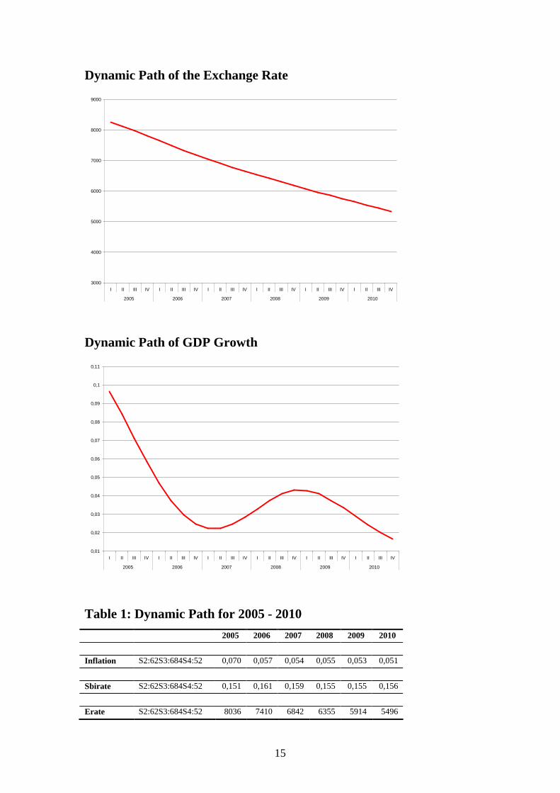
Dynamic Path of the Exchange Rate

3000

4000

5000

6000

7000

8000

9000


2005 2006 2007 2008 2009 2010

Dynamic Path of GDP Growth

0,01

0,02

0,03

0,04

0,05

0,06

0,07

0,08

0,09

0,1

0,11


2005 2006 2007 2008 2009 2010

Table 1: Dynamic Path for 2005 - 2010 2005 2006 2007 2008 2009 2010

Inflation S2:62S3:684S4:52 0,070 0,057 0,054 0,055 0,053 0,051

Sbirate S2:62S3:684S4:52 0,151 0,161 0,159 0,155 0,155 0,156

Erate S2:62S3:684S4:52 8036 7410 6842 6355 5914 5496

16

Gdpgrowth S2:62S3:684S4:52 0,074 0,032 0,019 0,027 0,033 0,031

3.2 Interest Rate Simulation using Soft and Hard Preferences

Since the interest rate is endogenously determined by the Taylor Reaction

Function, different interest rate simulation paths then can be attained through the

following steps:

1. Changing the weights of coefficients of the Taylor Reaction Function; or

2. Altering the time horizon in which the desired inflation target is to be

achieved.

The weighted coefficients will determine monetary policy responses to the

inflation gap, between the actual and target rates while a change in the time horizon

reflects aggressiveness of the disinflation program undertaken by the central bank.

17

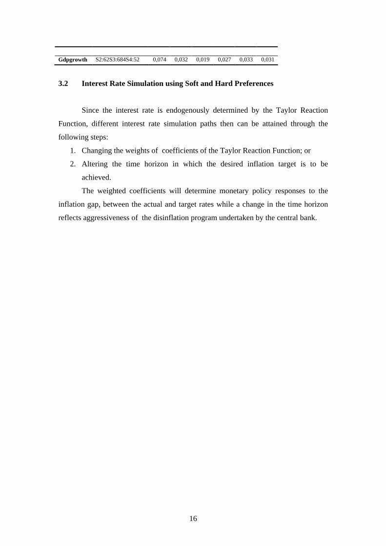
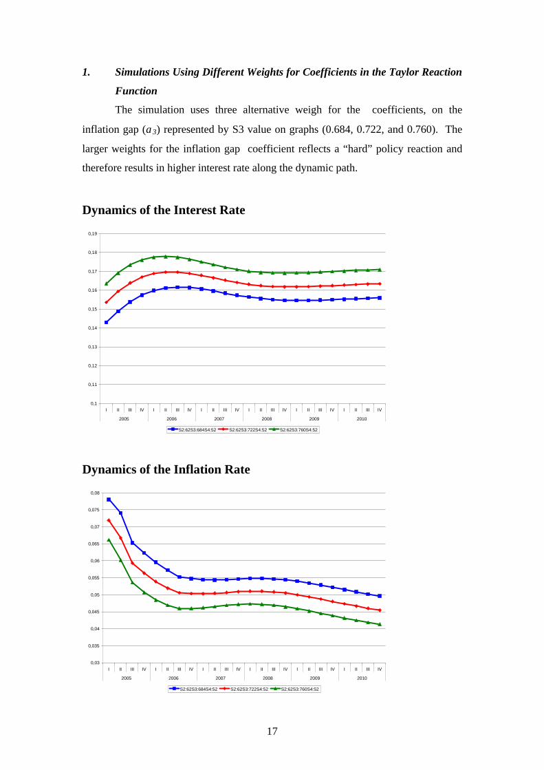
1. Simulations Using Different Weights for Coefficients in the Taylor Reaction

Function

The simulation uses three alternative weigh for the coefficients, on the

inflation gap (α3) represented by S3 value on graphs (0.684, 0.722, and 0.760). The

larger weights for the inflation gap coefficient reflects a “hard” policy reaction and

therefore results in higher interest rate along the dynamic path.

Dynamics of the Interest Rate

0,1

0,11

0,12

0,13

0,14

0,15

0,16

0,17

0,18

0,19


2005 2006 2007 2008 2009 2010

S2:62S3:684S4:52 S2:62S3:722S4:52 S2:62S3:760S4:52

Dynamics of the Inflation Rate

0,03

0,035

0,04

0,045

0,05

0,055

0,06

0,065

0,07

0,075

0,08


2005 2006 2007 2008 2009 2010

S2:62S3:684S4:52 S2:62S3:722S4:52 S2:62S3:760S4:52

18

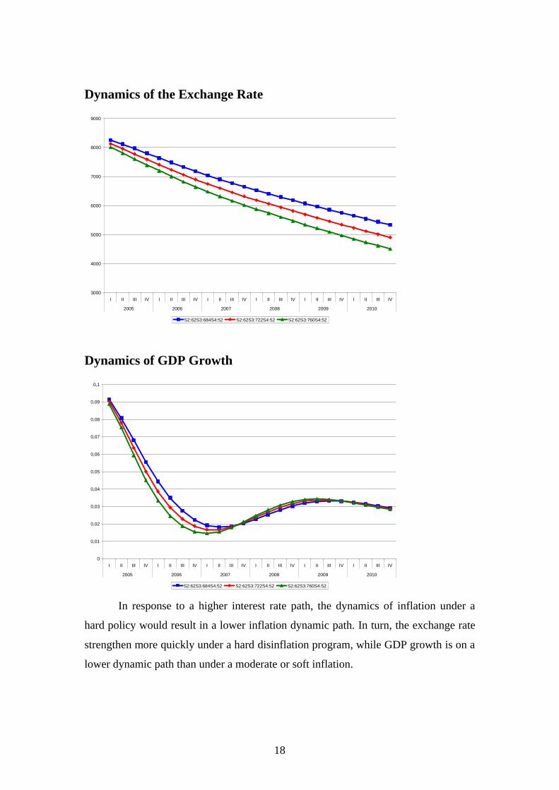
Dynamics of the Exchange Rate

3000

4000

5000

6000

7000

8000

9000


2005 2006 2007 2008 2009 2010

S2:62S3:684S4:52 S2:62S3:722S4:52 S2:62S3:760S4:52

Dynamics of GDP Growth

0

0,01

0,02

0,03

0,04

0,05

0,06

0,07

0,08

0,09

0,1


2005 2006 2007 2008 2009 2010

S2:62S3:684S4:52 S2:62S3:722S4:52 S2:62S3:760S4:52 In response to a higher interest rate path, the dynamics of inflation under a

hard policy would result in a lower inflation dynamic path. In turn, the exchange rate

strengthen more quickly under a hard disinflation program, while GDP growth is on a

lower dynamic path than under a moderate or soft inflation.

19

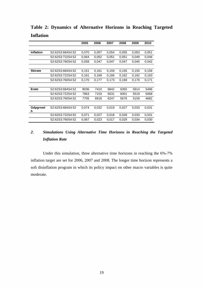
Table 2: Dynamics of Alternative Horizons in Reaching Targeted

Inflation 2005 2006 2007 2008 2009 2010 Inflation S2:62S3:684S4:52 0,070 0,057 0,054 0,055 0,053 0,051 S2:62S3:722S4:52 0,064 0,052 0,051 0,051 0,049 0,046 S2:62S3:760S4:52 0,058 0,047 0,047 0,047 0,045 0,042 Sbirate S2:62S3:684S4:52 0,151 0,161 0,159 0,155 0,155 0,156 S2:62S3:722S4:52 0,161 0,169 0,166 0,162 0,162 0,163 S2:62S3:760S4:52 0,170 0,177 0,173 0,169 0,170 0,171 Erate S2:62S3:684S4:52 8036 7410 6842 6355 5914 5496 S2:62S3:722S4:52 7863 7153 6531 6001 5519 5068 S2:62S3:760S4:52 7705 6918 6247 5676 5159 4682 Gdpgrowth

S2:62S3:684S4:52 0,074 0,032 0,019 0,027 0,033 0,031

S2:62S3:722S4:52 0,071 0,027 0,018 0,028 0,033 0,031 S2:62S3:760S4:52 0,067 0,023 0,017 0,029 0,034 0,030

2. Simulations Using Alternative Time Horizons in Reaching the Targeted

Inflation Rate

Under this simulation, three alternative time horizons in reaching the 6%-7%

inflation target are set for 2006, 2007 and 2008. The longer time horizon represents a

soft disinflation program in which its policy impact on other macro variables is quite

moderate.

20

Dynamics of Inflation

0

0,02

0,04

0,06

0,08

0,1

0,12

0,14


2005 2006 2007 2008 2009 2010

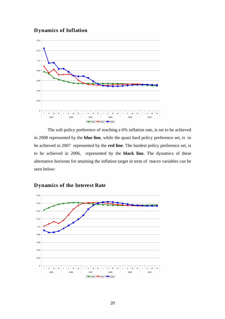
2006 2007 2008 The soft policy preference of reaching a 6% inflation rate, is set to be achieved

in 2008 represented by the blue line, while the quasi hard policy preference set, is to

be achieved in 2007 represented by the red line. The hardest policy preference set, is

to be achieved in 2006, represented by the black line. The dynamics of these

alternative horizons for attaining the inflation target in term of macro variables can be

seen below:

Dynamics of the Interest Rate

0

0,02

0,04

0,06

0,08

0,1

0,12

0,14

0,16

0,18


2005 2006 2007 2008 2009 2010

2006 2007 2008

21

The soft disinflation program allows a longer time horizon in reaching the targeted

inflation rate, and, as a result, it requires lower interest rate dynamics (blue line). The

average interest rate level moves around 8.8% in 2005, 10.7% in 2006 and 14.7% in 2007 and

eventually ends up in a narrowing range of between 14%-16%..

The responses in monetary policy required by the quasi hard disinflation

program create higher interest rate dynamic path. The average SBI rate moves from

around 15.1% in 2005 to 16.1% in 2006, and to 15.9% in 2007 and ends up in

narrowing range as well (red line). Similarly, the hardest disinflation program leads to

a much higher interest rate dynamic path as is reflected in the black line.

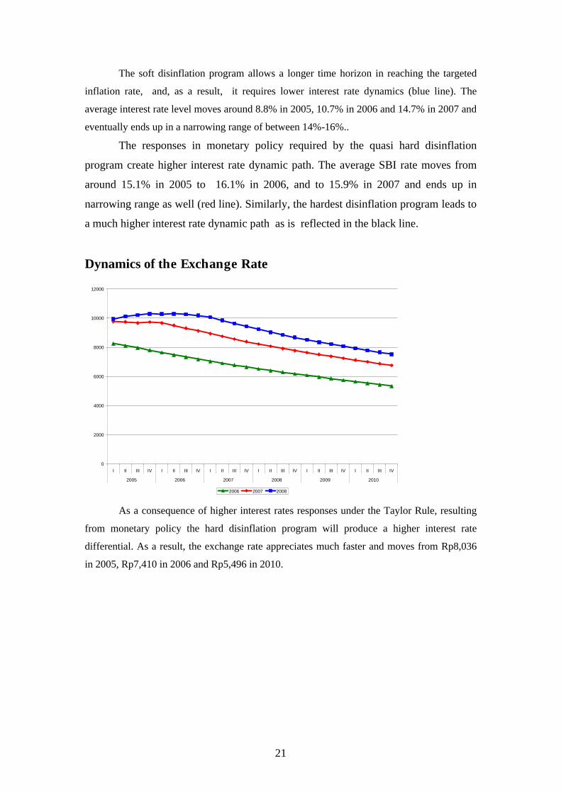
Dynamics of the Exchange Rate

0

2000

4000

6000

8000

10000

12000


2005 2006 2007 2008 2009 2010

2006 2007 2008 As a consequence of higher interest rates responses under the Taylor Rule, resulting

from monetary policy the hard disinflation program will produce a higher interest rate

differential. As a result, the exchange rate appreciates much faster and moves from Rp8,036

in 2005, Rp7,410 in 2006 and Rp5,496 in 2010.

22

Dynamics of GDP Growth

-0,02

0

0,02

0,04

0,06

0,08

0,1

0,12

0,14

0,16


2005 2006 2007 2008 2009 2010

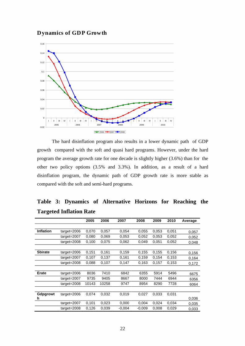
2006 2007 2008 The hard disinflation program also results in a lower dynamic path of GDP

growth compared with the soft and quasi hard programs. However, under the hard

program the average growth rate for one decade is slightly higher (3.6%) than for the

other two policy options (3.5% and 3.3%). In addition, as a result of a hard

disinflation program, the dynamic path of GDP growth rate is more stable as

compared with the soft and semi-hard programs.

Table 3: Dynamics of Alternative Horizons for Reaching the

Targeted Inflation Rate 2005 2006 2007 2008 2009 2010 Average Inflation target=2006 0,070 0,057 0,054 0,055 0,053 0,051 0,057 target=2007 0,080 0,069 0,053 0,052 0,053 0,052 0,052 target=2008 0,100 0,075 0,062 0,049 0,051 0,052 0,048 Sbirate target=2006 0,151 0,161 0,159 0,155 0,155 0,156 0,156 target=2007 0,107 0,137 0,161 0,159 0,154 0,153 0,164 target=2008 0,088 0,107 0,147 0,163 0,157 0,153 0,172 Erate target=2006 8036 7410 6842 6355 5914 5496 6675 target=2007 9735 9405 8667 8000 7444 6944 6356 target=2008 10143 10258 9747 8954 8290 7728 6064 Gdpgrowth

target=2006 0,074 0,032 0,019 0,027 0,033 0,031 0,036

target=2007 0,101 0,023 0,000 0,004 0,024 0,034 0,035 target=2008 0,126 0,039 -0,004 -0,009 0,008 0,029 0,033

23

4. Conclusion

• Alternative simulations using GEMBI provide the dynamic impacts of different

disinflation programs on other macroeconomic variables. Under different central

bank preferences (play soft or play hard) one would be able to see different

desired paths of interest rates responses to achieve the medium-term inflation

target and its impact on the exchange rate and GDP growth rate.

• The “soft” disinflation program (both in the form of a longer achievement horizon

and in lower coefficient weight in the Taylor Rule reaction function) turn out to

have moderate positive impacts on interest rate dynamics and GDP growth.

• The “hard” disinflation program, as reflected in the shorter achievement horizon

or in the bigger weight in Taylor Rule reaction function, did exactly reflect a

lowering of the GDP growth path in the first two years but gradually achieves a

higher growth rate of GDP in the following years as compared to the other

disinflation programs.

24

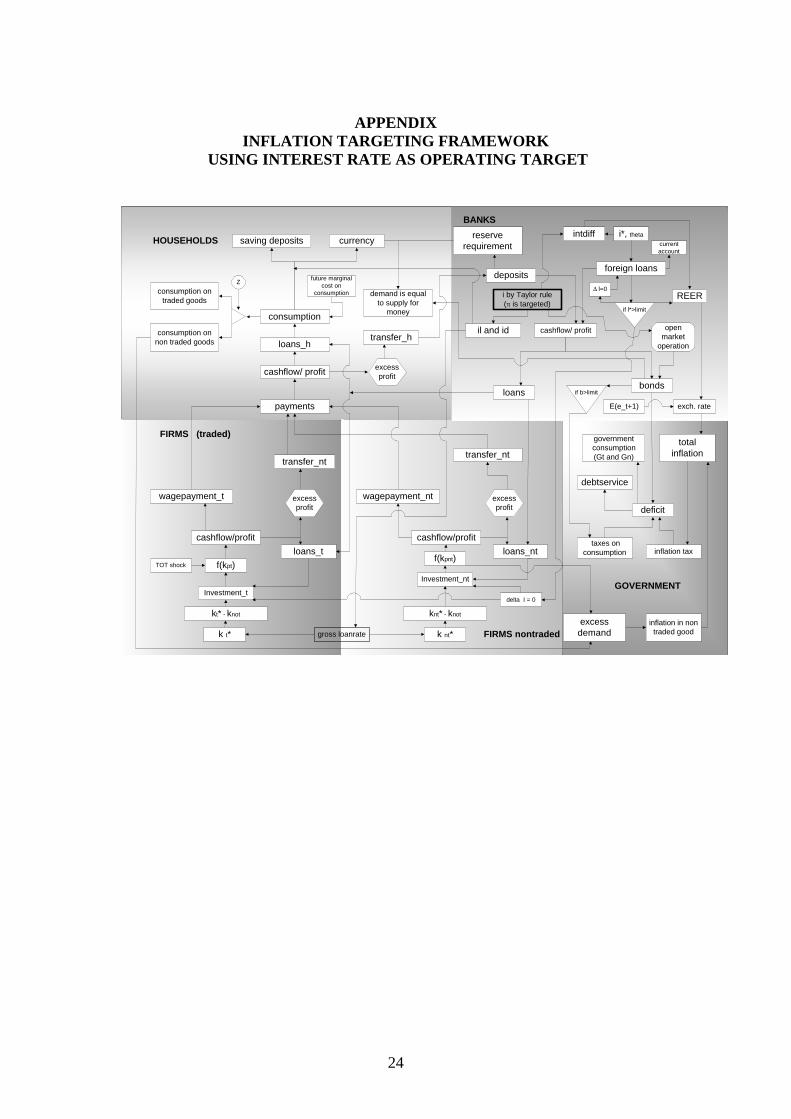
APPENDIX

INFLATION TARGETING FRAMEWORK USING INTEREST RATE AS OPERATING TARGET

excessdemand

totalinflation

intdiff

i by Taylor rule(π is targeted)

FIRMS (traded)

FIRMS nontraded

HOUSEHOLDS

BANKS

GOVERNMENT

gross loanratek t* k nt*

kt* - knot knt* - knot

Investment_t

Investment_nt

f(kpt)f(kpnt)

cashflow/profit cashflow/profit

wagepayment_t

transfer_nt

wagepayment_nt

transfer_nt

payments

excessprofit

loans_t

excessprofit

loans_nt

cashflow/ profit

loans_htransfer_h

consumption

consumption ontraded goods

consumption onnon traded goods

currencysaving deposits

cashflow/ profit

depositsforeign loans

bonds

reserverequirement

demand is equalto supply for

money

loans

REER

inflation in nontraded good

openmarket

operation

if l*>limit

i*, theta

deficit

governmentconsumption(Gt and Gn)

taxes onconsumption inflation tax

debtservice

exch. rateE(e_t+1)

TOT shock

excessprofit

il and id

if b>limit

Zfuture marginal

cost onconsumption

delta I = 0

∆ l=0

currentaccount

25

References 1. Agenor, Pierre and Peter Montiel (2000), “Development Macroeconomics”,

second edition, Princeton, N.J. Princeton University Press. 2. Den Haan.W. dan A.Marcet (1990), “Solving the Stochastic Growth Model by

Parameterizing Expectations”, Journal of Business and Economics Statistics 8,p.31-34.

3. Den Haan.W. & A.Marcet (1994), “Accuracy in Simulations”, Review of Economic Studies 61,p.3-17.

4. Diebold, Francis X.,”The Past, Present, and Future of Macroeconomic Forecasting”, University of Pennsylvania and NBER, October 22, 1997 in Journal of Economics Perspective (1998) 12: 175-192.

5. Duffy, John dan Paul D.McNelis (2000), “Approximating and Simulating the Stochastic Growth Model: Parameterized Expectations, Neural Networks and the Genetic Algorithm”.Journal of Economic Dynamics and Control. Website: www.georgetown.edu/mcnelis.

6. Kydland, Finn E. and Edward C. Prescott, “The Computational Experiment: An Econometric Tool”, Federal Reserves Bank of Minneapolis, Research Department Staff Report 178, August 1994.

7. Marcet, A.(1988), “Solving Nonlinear Models by Parameterizing Expectations”, Working Paper, Graduate School of Industrial Administration, Carnegie Mellon University.

8. McCallum, B., “Recent Developments in the Analysis of Monetary Policy Rules”, Federal Reserves Bank of St.Louis Review, November/December 1999.

9. McNelis, Paul D., “Computational Macrodynamics for Emerging Market Economies”, Department of Economics, Georgetown University, Washington DC, August 2000.

10. McNelis, Paul D.,”Inflation Targeting in Emerging Market Economies: A General Equilibrium Model for Bank Indonesia”, Department of Economics, Georgetown University, Washington DC, August 2000.

11. Mendoza, Enrique G (1995), “The Terms of Trade, the Real Exchange Rate, and Economic Fluctuations”, International Economic Review 36: 101-137.

12. Sawyer, John A., “Macroeconomic Theory: Keynesian and New Walrasian Models”, University of Pennsylvania Press, Philadelphia, 1989.

13. Sims, Christopher (2000), “Solving Linear Rational Expectations Models”, Manuscript, Department of Economics, Princeton University.

playing hard or soft? : a simulation of indonesian ... filecharles joseph, janu dewandaru, iman...

Documents