pitchfork bifurcations of invariant manifolds - core.ac.uk · topology and its applications 154...
TRANSCRIPT
Topology and its Applications 154 (2007) 1650–1663
www.elsevier.com/locate/topol
Pitchfork bifurcations of invariant manifolds
Jyoti Champanerkar a,∗, Denis Blackmore b
a Department of Mathematics and Statistics, University of South Alabama, Mobile, AL 36688, USAb Department of Mathematical Sciences, New Jersey Institute of Technology, Newark, NJ 07102, USA
Received 2 June 2006; received in revised form 25 December 2006; accepted 25 December 2006
Abstract
A pitchfork bifurcation of an (m − 1)-dimensional invariant submanifold of a dynamical system in Rm is defined analogous
to that in R. Sufficient conditions for such a bifurcation to occur are stated and existence of the bifurcated manifolds is provedunder the stated hypotheses. For discrete dynamical systems, the existence of locally attracting manifolds M+ and M−, after thebifurcation has taken place is proved by constructing a diffeomorphism of the unstable manifold M . Techniques used for provingthe theorem involve differential topology and analysis. The theorem is illustrated by means of a canonical example.© 2007 Elsevier B.V. All rights reserved.
Keywords: Bifurcation; Pitchfork bifurcation; Invariant manifolds
1. Introduction
Pitchfork bifurcations bear the name due to the fact that the bifurcation diagram for a one-parameter family inR looks like a pitchfork. The pitchfork bifurcation for a fixed point in R has been widely studied (see, e.g., [17]).In R, sufficient conditions for the occurrence of a pitchfork bifurcation of a non-hyperbolic fixed point are stated,for instance, in [20,23]. A generalization of the result in R is given by Sotomayor’s theorem [19] for a pitchforkbifurcation of a fixed point in R
n. Another generalization for pitchfork bifurcations is that for a periodic orbit [19].Analytical discussions of pitchfork (or pitchfork type) bifurcations can be found for particular classes of dynamicalsystems, e.g., [10], where a quasi-periodically forced map is studied. Interesting numerical analyses of pitchforkbifurcations can be found in [18,22].
An algorithm to compute invariant manifolds of equilibrium points and periodic orbits is presented in [16]. It isimportant to study invariant manifolds in order to better understand the global dynamics of a system. The classicalpitchfork bifurcation concerns a fixed point (invariant codimension-1 submanifold) on the real line, possibly after astandard (Lyapunov–Schmidt) reduction procedure. From a mathematical viewpoint, it is therefore natural and im-portant to investigate higher dimensional extensions of this theorem to invariant codimension-1 submanifolds of aEuclidean m-space. Such considerations have applications for a variety of cases arising from perturbations of dy-
* Corresponding author.E-mail address: [email protected] (J. Champanerkar).
0166-8641/$ – see front matter © 2007 Elsevier B.V. All rights reserved.doi:10.1016/j.topol.2006.12.014
J. Champanerkar, D. Blackmore / Topology and its Applications 154 (2007) 1650–1663 1651
namical systems having sufficiently regular first integrals. Examples include perturbations of standard models forpopulation dynamics (e.g., [3,14]), and particular forms of dissipative perturbations (corresponding to real fluid vis-cous effects) of ideal fluid motion involving highly concentrated vorticity fields such as in [2]. Accordingly we askunder what conditions an invariant manifold of a (discrete or continuous) dynamical system undergoes a bifurcationof pitchfork type? A fairly complete answer to this question is provided in this work. We give sufficient conditions forthe occurrence of a pitchfork type bifurcation of a compact, boundaryless, codimension-1, invariant manifold in R
m.Our criteria involve essentially only estimates for the norms of certain partial derivatives, and are independent of the
finer details of the dynamics on the invariant manifold. This is at once a strength and weakness of our main theorems.It is a strength inasmuch as we do not have to be concerned with the dynamics restricted to the invariant manifold. Itis a weakness in that by not using additional properties of the restricted systems, our results are not as sharp as theymight otherwise be, and we are not able to guarantee that the restricted dynamics are in any way invariant during thebifurcation such as in the related work of Broer and his collaborators (e.g., [4–6]), Chenciner [7–9], and Aronson etal. [1]. In any case, we do obtain readily verifiable criteria for identifying such bifurcations, and illustrate the use ofthese criteria in an example. Techniques used for proving the theorem involve differential topology and analysis andare adapted from Hartman [12], Hirsch et al. [13] and Shub [21].
2. Definitions
Let M be a codimension-1, compact, connected, boundaryless submanifold of Rm. By the Jordan–Brouwer sepa-
ration theorem [11], M divides Rm\M into an outer unbounded region and an inner bounded region. We shall study
C1 functions F :U × (−a, a) → Rm, where U is an open neighborhood of M in R
m and (−a, a), a > 0, is an opensymmetric interval of real numbers. It shall be assumed in the sequel that each of the maps Fμ :U → R
m, |μ| < a, isa C1 diffeomorphism and that M is Fμ-invariant, i.e., Fμ(M) = M .
Definition 1. With M and Fμ as above, we say that Fμ is side-preserving if for every x in the inner bounded region,Fμ(x) also lies in the inner region.
Definition 2. With M and Fμ as above, we say that Fμ is side-reversing if for every x in the inner bounded region,Fμ(x) lies in the outer unbounded region.
Note that if Fμ is a diffeomorphism of a neighborhood of M and leaves M invariant, then Fμ is either side-preserving or side-reversing. Analogous to the definition of a pitchfork bifurcation in R, we define a pitchforkbifurcation of invariant manifolds in R
m as follows.
Definition 3. Consider a discrete dynamical system in Rm given by xn+1 = Fμ(xn). Let M be an invariant manifold
for all μ ∈ (−a, a). If 0 � μ0 < a is such that M is locally attracting (repelling) for μ < 0, M is locally repelling(attracting) for μ > μ0 and in addition two locally attracting (repelling) Fμ-invariant diffeomorphic copies of M ,viz., M− and M+ appear in a small neighborhood of M for μ > μ0, then we say that M has undergone a pitchforkbifurcation at μ0.
In the definition above, it does not matter what happens in the interval (0,μ0). It is typically assumed that theinterval (0,μ0) is small. In R, 0 coincides with μ0, since the manifold under consideration is just a single point. Butfor higher dimensions, not all points on the invariant manifold may undergo a change in stability at the same value ofthe parameter μ. When μ � μ0, all the points have changed stability and two new invariant, diffeomorphic copies ofthe original manifold (of opposite stability) appear.
3. Pitchfork bifurcation theorem for discrete dynamical system
We consider (one-parameter families of) discrete dynamical systems given by
xn+1 = F(xn,μ), (3.1)
1652 J. Champanerkar, D. Blackmore / Topology and its Applications 154 (2007) 1650–1663
where xn ∈ Rm for every n ∈ N and μ ∈ (−a, a) ⊆ R. Additional properties of F(·,μ), also denoted as Fμ(·) are
described later. Let M be a compact, connected, boundaryless, codimension-1, C1 submanifold of Rm, which is Fμ-
invariant ∀μ ∈ (−a, a). Denote a tubular neighborhood of M as N(α) = {x ∈ Rm: d(x,M) � α,α > 0}, where d is
the standard Euclidean distance function. Assume that α is sufficiently small so that the ε-neighborhood theorem [11]can be applied and N(α) ⊂ U . This means that every element x ∈ N(α) can be uniquely represented as x = (r, y)
where y = π(x) ∈ M is the point on M closest to x and r ∈ [−α,α] is the signed distance in the outward normaldirection between x and M . We also assume that Fμ(N(α)) ⊂ N(α). This enables us to write Fμ in component formas Fμ = (fμ,gμ) where fμ :N(α) → R, gμ = π ◦ Fμ :N(α) → M , and fμ(x) is the signed distance from gμ(x) toFμ(x). Observe that F−1
μ (Fμ(N(α))) = N(α), so that F−1μ can be written in component form as F−1
μ = (fμ, gμ).We shall use standard notation for derivatives and partial derivatives of functions. For example, the derivative of
Fμ :N(α) → Rm will be denoted by DFμ, and represented as the usual m × m Jacobian matrix
DFμ(r, y) =[
Drfμ(r, y) Dyfμ(r, y)
Drgμ(r, y) Dygμ(r, y)
],
where the entries are submatrices representing the partial derivatives such as
Drfμ(r, y) = ∂fμ
∂r(r, y) and Dygμ(r, y) =
[∂gμi
∂yj
](m−1)×(m−1)
.
We use | · | for the Euclidean norm of an element of a Euclidean space or the associated norm of a linear mapping(matrix) between Euclidean spaces. The symbol ‖·‖ denotes the supremum norm of a function taking values in aEuclidean space or in a space of linear transformations of Euclidean spaces taken over an appropriate set, which issometimes indicated as a subscript of the norm.
If the rate of change (with respect to r) in the normal component fμ in the radial direction r is strictly less than 1 inabsolute value, the manifold M will be locally attracting. This is stated mathematically in statement (2) of Theorem 4,which follows. Similarly to have M locally repelling, we require that |Drfμ| be greater than one as in statement (3).Statements (4) and (5) describe locally attracting properties in a neighborhood away from M , which is where our newbifurcated manifolds M− and M+ will reside. Properties (6) and (7) are obtained analytically and are needed in orderto establish the existence of manifolds M− and M+ as graphs of a fixed point (Lipschitz function) in a Banach space.The last hypothesis (statement (8)) provides boundedness and equicontinuity properties that enable us to bootstrapLipschitz homeomorphisms of M with M+ and M− up to C1 diffeomorphisms. These ideas shall become clear as theproof unfolds and after the remarks following the proof.
Theorem 4. With Fμ and M as above, suppose that the following statements hold:
(1) Fμ is side-preserving for every μ ∈ (−a, a).(2) sup(r,y)∈N(α) |Drfμ(r, y)| = ‖Drfμ‖N(α) < 1 for every μ ∈ (−a,0).(3) ∃0 < μ� < a such that infy∈M |Drfμ(0, y)| > 1 ∀μ ∈ (μ�, a).(4) ∃0 < α1 < α such that ‖Drfμ(r, y)‖A < 1 ∀μ ∈ [0, a), where A = {x ∈ R
m: α1 � d(x,M) � α} and ‖.‖A is thesup norm over A.
(5) ∃χ : [0, a) → R continuous with 0 � χ(μ) � α1 and K(μ) := {x ∈ Rm: χ(μ) � d(x,M) = d(x, y) � α} such
that Fμ(K(μ)) ⊆ K(μ) for all μ ∈ (μ�, a). Furthermore c(μ) := ‖Drfμ‖K(μ) < 1 ∀μ ∈ (μ�, a), where ‖.‖K(μ)
is defined to be the sup norm over K(μ).(6) c�(μ) := (‖Drfμ‖K(μ))(1 + ‖Drgμ‖K(μ)) + ‖Dyfμ‖K(μ)‖Drg‖K(μ) < 1 for each μ ∈ (μ�, a), where ‖.‖K(μ) is
defined to be the sup norm over K(μ). Here (fμ, gμ) denotes the inverse map F−1μ .
(7) (‖Drfμ‖K(μ) + ‖Dyfμ‖K(μ))(‖Drgμ‖K(μ) + ‖Dygμ‖K(μ)) � 1 for each μ ∈ (μ�, a).(8) σ(μ) := ‖Drfμ‖K(μ)(2‖Drgμ‖K(μ) + ‖Dygμ‖K(μ)) + ‖Dyfμ‖K(μ)‖Drgμ‖K(μ) < 1 for all μ ∈ (μ�, a).
Then for each μ ∈ (μ�, a), ∃ codimension-1 submanifolds M+(μ) and M−(μ) in K(μ) such that both M+(μ)
and M−(μ) are Fμ-invariant, locally attracting and C1 diffeomorphic to M . M is locally repelling, and r > 0 for allx = (r, y) ∈ M+, and r < 0 for all x = (r, y) ∈ M−.
J. Champanerkar, D. Blackmore / Topology and its Applications 154 (2007) 1650–1663 1653
Proof. Recall that N(α) = {x = (r, y) ∈ Rm: |r| = d(x,M) � α, y = π(x)}. Now Fμ(r, y) = (fμ(r, y), gμ(r, y)) in
component form where, fμ :N(α) → R is the signed distance between Fμ(r, y) and gμ(r, y) and gμ :N(α) → M isthe projection π ◦ Fμ(y) of Fμ(r, y) on M . We shall break the proof up into a number of steps (claims).
Claim 1. M is locally attracting for μ ∈ (−a,0).
Proof of Claim 1. Consider a point (r0, y0) ∈ N(α). Let (rn, yn) be the point obtained by applying the n-fold com-position of Fμ with itself to (r0, y0). Then
(rn, yn) = Fμ(rn−1, yn−1) = (fμ(rn−1, yn−1), gμ(rn−1, yn−1)
)implies that
d((rn, yn),M
) = d((rn, yn),π(rn, yn)
) = fμ(rn−1, yn−1).
As M is Fμ-invariant, it follows that fμ(0, yn−1) = 0 for all n ∈ N. So,
|rn| =∣∣fμ(rn−1, yn−1)
∣∣ = ∣∣fμ(rn−1, yn−1) − fμ(0, yn−1)∣∣ =
∣∣∣∣∂fμ(r�, yn−1)
∂r
∣∣∣∣|rn−1|
for some r� such that 0 � r� < rn−1, by the mean value theorem. Thus |rn| < c|rn−1| < cn|r0|, where c =sup(r,y)∈N(α) |∂fμ(r, y)/∂r| < 1 by property (2). Therefore, rn → 0 as n → ∞. Consequently d((rn, yn),M) → 0.That is, for any initial point (r0, y0) in the neighborhood N(α) of M , Fn
μ(r0, y0) converges to M . It follows that M islocally attracting for all μ ∈ (−a,0).
Claim 2. M is locally repelling for μ ∈ (μ�, a).
Proof of Claim 2. Following the same steps as above, we find that |rn| > c|rn−1| > |rn−1| whenever |rn| is suffi-ciently small owing to statement (3). Accordingly the iterates {xn} must eventually leave any sufficiently thin tubularneighborhood of M for μ ∈ (μ�, a), which means that M is locally repelling. We now fix a μ ∈ (μ�, a) and suppressμ in the notation for simplicity. To begin with, we shall prove the existence of M+ as an Fμ-invariant manifold home-omorphic to M . It suffices to prove the existence of M+, as the existence of M− can be established in the same way.Observe that M+ is invariant iff F(M+) = M+. We shall seek M+ in the form of the graph of a continuous functionover M defined as
M+ = Γψ = {(ψ(y), y
): y ∈ M
},
where M+ ⊂ K = K(μ), ψ :M → R and ψ(y) � 0 for all y ∈ M . Then for all y ∈ M , we have that (ψ(y), y) ∈ M+iff F(ψ(y), y) = (ψ(z), z) ∈ M+, which is equivalent to(
f(ψ(y), y
), g
(ψ(y), y
)) = (ψ(z), z
) ∈ M+. (3.2)
F is a diffeomorphism, hence F−1(ψ(z), z) = (ψ(y), y) which implies that(f
(ψ(z), z
), g
(ψ(z), z
)) = (ψ(y), y
), (3.3)
where F−1 = (f , g). Combining Eqs. (3.2) and (3.3), we find that M+ is invariant iff ψ satisfies the functionalequation
ψ(z) = f(ψ
(g(ψ(z), z)
), g
(ψ(z), z
)). (3.4)
Let Lip(A,B) denote the set of all Lipschitz functions from A to B . Let L(ψ) denote the Lipschitz constant of aLipschitz function ψ , and Γψ = {(ψ(y), y): y ∈ M} denote the graph of ψ . Now define the set
X := {ψ ∈ Lip
(M,R
+ ∪ {0}): L(ψ) � 1,Γψ ⊆ K}.
Claim 3. {X,‖ · ‖K} is a Banach space.
1654 J. Champanerkar, D. Blackmore / Topology and its Applications 154 (2007) 1650–1663
Proof of Claim 3. Let {ψn} be a Cauchy sequence in X. Then for all n ∈ N we have that ψn :MLip−−→ R
+ ∪ {0},L(ψn) � 1 and Γψn ∈ K(μ). Here Γψn denotes the graph of ψn over M . Since the sequence {ψn} is Lipschitz, everyψn is continuous. Now M is compact and R
+ ∪ {0} is closed, so the set of all continuous functions from M toR
+ ∪ {0} with sup norm forms a Banach space. Moreover, if ψn → ψ as n → ∞, it is clear that ψ is also Lipschitz,with Lipschitz constant not greater than one. To see this, note that given any ε > 0, there exists n0 ∈ N such that‖ψn − ψ‖sup < ε for all n � n0. Let N > n0. Then we have∣∣ψ(y1) − ψ(y2)
∣∣= ∣∣ψ(y1) − ψN(y1) + ψN(y1) − ψN(y2) + ψN(y2) − ψ(y2)
∣∣�
∣∣ψ(y1) − ψN(y1)∣∣ + ∣∣ψN(y1) − ψN(y2)
∣∣ + ∣∣ψN(y2) − ψ(y2)∣∣
� ε + |y1 − y2| + ε
using the fact that ψn → ψ and that ψN is Lipschitz with L(ψ) � 1. That is,∣∣ψ(y1) − ψ(y2)∣∣ � 2ε + |y1 − y2| ∀ε > 0.
Since ε > 0 is arbitrarily small, it follows that∣∣ψ(y1) − ψ(y2)∣∣ � |y1 − y2|,
so ψ ∈ Lip(M,R+ ∪ {0}) and L(ψ) � 1.
Since K is closed, K contains all its limit points. Therefore Γψn ∈ K for all n implies that
limn→∞Γψn = lim
n→∞(ψn(y), y
) = (ψ(y), y
) = Γψ ∈ K,
hence X is a Banach space. In view of (3.4), we define an operator F on X as follows.
F(ψ)(y) := f(ψ
(g(ψ(y), y)
), g
(ψ(y), y
)). (3.5)
Claim 4. F(X) ⊆ X.
Proof of Claim 4. Let z = g(ψ(y), y). Then f (ψ(z), z) = signed distance between F(ψ(z), z) and π(F(ψ(z), z)).If ψ(z) > 0, then f (ψ(z), z) > 0 since F is side-preserving. So F(ψ) is indeed a function from M to R
+ ∪{0}. F(ψ)
is continuous since it is a composition of continuous functions. Now it follows from the mean value theorem and thedefinition of X that∣∣F(ψ)(y1) −F(ψ)(y2)
∣∣ = ∣∣f (ψ(z1), z1) − f (ψ(z2), z2)∣∣
�∥∥∥∥∂f
∂r
∥∥∥∥K
∣∣ψ(z1) − ψ(z2)∣∣ + ‖Dyf ‖K |z1 − z2|
�(∥∥∥∥∂f
∂r
∥∥∥∥K
+ ‖Dyf ‖K
)|z1 − z2|,
where ‖ .‖K = sup{|.|: (r, y) ∈ K}. The above inequality follows because ψ is a Lipschitz function with Lipschitzconstant � 1. Also
|z1 − z2| =∣∣g(
ψ(y1), y1) − g
(ψ(y2), y2
)∣∣� ‖Drg‖K
∣∣ψ(y1) − ψ(y2)∣∣ + ‖Dyg‖K |y1 − y2|
�(‖Drg‖K + ‖Dyg‖K
)|y1 − y2|.The two inequalities obtained above, together with property (7) imply that
∣∣F(ψ)(y1) −F(ψ)(y2)∣∣ �
(∥∥∥∥∂f
∂r
∥∥∥∥K
+ ‖Dyf ‖K
)(‖Drg‖K + ‖Dyg‖K
)|y1 − y1| � |y1 − y2|.
Therefore, F(ψ) ∈ Lip(M,R+ ∪ {0}) and L(F(ψ)) � 1. We will now prove that F is a contraction mapping. Using
statement (6) and the mean value theorem, we compute that
J. Champanerkar, D. Blackmore / Topology and its Applications 154 (2007) 1650–1663 1655
∣∣F(ψ1)(y) −F(ψ2)(y)∣∣
= ∣∣f (ψ1
(g(ψ1(y), y)
), g(ψ1(y), y)
) − f(ψ2
(g(ψ2(y), y)
), g(ψ2(y), y)
)∣∣�
∥∥∥∥∂f
∂r
∥∥∥∥K
∣∣ψ1(g(ψ1(y), y)
) − ψ2(g(ψ2(y), y)
)∣∣ + ‖Dyf ‖K
∣∣g(ψ1(y), y) − g(ψ2(y), y)∣∣
�∥∥∥∥∂f
∂r
∥∥∥∥K
∣∣ψ1(g(ψ1(y), y)
) − ψ1(g(ψ2(y), y)
)∣∣
+∥∥∥∥∂f
∂r
∥∥∥∥K
∣∣ψ1(g(ψ2(y), y)
) − ψ2(g(ψ2(y), y)
)∣∣ + ‖Dyf ‖K
∣∣g(ψ1(y), y) − g(ψ2(y), y)∣∣
�∥∥∥∥∂f
∂r
∥∥∥∥K
(∣∣g(ψ1(y), y) − g(ψ2(y), y)∣∣ + ‖ψ1 − ψ2‖
) + ‖Dyf ‖K
∣∣g(ψ1(y), y) − g(ψ2(y), y)∣∣
�∥∥∥∥∂f
∂r
∥∥∥∥K
(‖Drg‖K‖ψ1 − ψ2‖ + ‖ψ1 − ψ2‖) + ‖Dyf ‖K‖Drg‖K‖ψ1 − ψ2‖
={∥∥∥∥∂f
∂r
∥∥∥∥K
(1 + ‖Drg‖K
) + ‖Dyf ‖K
}‖ψ1 − ψ2‖.
This is true for all y ∈ M . Hence it is true for the supremum with y taken over M ; therefore, we obtain the relation
∥∥F(ψ1) −F(ψ2)∥∥ �
[∥∥∥∥∂f
∂r
∥∥∥∥K
(1 + ‖Drg‖K
) + ‖Dyf ‖K
]‖ψ1 − ψ2‖,
∥∥F(ψ1) −F(ψ2)∥∥ � c�‖ψ1 − ψ2‖,
where c� = ‖∂f/∂r‖K(1 + ‖Drg‖K) + ‖Dyf ‖K is such that 0 < c� < 1 by hypothesis (4). This implies that F(ψ) ∈Lip(M,R
+ ∪{0}) and that L(F(ψ)) < 1. We note here that the invariance of M implies that f (0, y) = f (0, y) = 0 forall (0, y) ∈ M . Accordingly Dyf (0, y) = Dyf (0, y) = 0 whenever x = (0, y) ∈ M , which means that both ‖Dyf ‖K
and ‖Dyf ‖K can be made as small as we like by choosing a sufficiently thin tubular neighborhood of M . Note that ifF(ψ(y), y) = (ψ(z), z), then (ψ(y), y) = F−1(ψ(z), z), and it follows that
ψ(y) = f(ψ(z), z
)and y = g
(ψ(z), z
).
Now consider ψ ∈ X. By definition, we have
ΓF(ψ) = {(F(ψ)(z), z): z ∈ M
}= {(
f(ψ(g(ψ(z), z)), g(ψ(z), z)
), z
): z ∈ M
}.
Moreover, F−1(ψ(z), z) = (ψ(y), y) ∈ K since F is a diffeomorphism, and F−1(N(α)) ⊂ N(α). The property thatΓψ ⊆ K implies that (ψ(z), z) ∈ K for every z, an element of M . Whence g(ψ(z), z) = y. This implies that
ΓF(ψ) = {(f (ψ(y), y), z
): z ∈ M
}= {(
f (ψ(y), y), g(ψ(y), y)): g
(ψ(y), y
) ∈ M}
= {(f (ψ(y), y), g(ψ(y), y)
): y ∈ M
}= {
F(ψ(y), y
): y ∈ M
}.
We know that (ψ(y), y) ∈ K for all y ∈ M and F(K) ⊆ K . This implies that ΓF(ψ) ⊆ K , thereby proving theclaim that F(X) ⊆ X. Hence F :X → X is a contraction mapping with respect to the sup norm on X. Since F is acontraction on a complete metric space X, it has a unique fixed point in X owing to Banach’s fixed point theorem. Letφ be the fixed point of F . Then φ ∈ Lip(M,R
+ ∪{0}) with Lipschitz constant L(φ) � 1, and φ satisfies the functionalequation (3.4). Therefore,
φ(z) = f(φ(g(φ(z), z)
), g
(φ(z), z
)). (3.6)
Claim 5. M+ exists and is locally attracting.
1656 J. Champanerkar, D. Blackmore / Topology and its Applications 154 (2007) 1650–1663
Proof of Claim 5. We now define M+ as the graph of φ as follows
M+ = Γφ = {(φ(y), y
): y ∈ M
},
where φ is as above. This proves the existence of M+. That M+ is locally attracting follows directly from its definitionas the graph of a fixed point (function) of a contraction mapping.
Claim 6. M+ is homeomorphic to M .
Proof of Claim 6. Let H :M → M+ be defined as H(y) := (φ(y), y). Then H is injective, surjective and continuous.H−1 exists and is also injective and surjective (bijective). Since M+ is compact, H−1 is also continuous. Hence themanifold M+ is homeomorphic to M .
Claim 7. The function φ is a class C1 map.
Proof of Claim 7. We know that φ is the solution to the functional equation (3.4), hence φ(z) = f (φ(g(φ(z), z)),g(φ(z), z)), φ ∈ Lip(M,R
+ ∪ {0}), and L(φ) � 1. We will inductively construct a sequence of C1 functions ψn whichconverges to φ. Then using the Arzela–Ascoli theorem, we will prove that φ is C1. The details are as follows. Chooseψ1 to be a positive constant such that Γψ1 ⊂ K . By construction, ψ1 is C1 and L(ψ1) = 0. Now suppose ψn is definedand that ψn is C1 with L(ψn) � 1. We define ψn+1 inductively as,
ψn+1(z) = F(ψn)(z) = f(ψn
(g(ψn(z), z)
), g
(ψn(z), z
)). (3.7)
Let hn :M → Rm denote the function (ψn, Id), where Id denotes the identity map on the second coordinate. That is,
hn(z) = (ψn(z), z). Then hn is C1 by the induction hypothesis and the fact that it is the composition of C1 maps, and
ψn+1(z) = f ◦ hn ◦ g ◦ hn(z).
Here we have used the fact that both f and g are C1 since F and F−1 are C1 diffeomorphisms. The sequence offunctions {ψn(z)} converges uniformly to φ(z) since φ satisfies the contractive functional equation (3.4). The Jacobianof ψn+1 evaluated at z is the 1 × (m − 1) matrix or the gradient vector of ψn+1 given as
Dψn+1(z) = Df(hn
(g(hn(z))
))Dhn
(g(hn(z)
))Dg
(hn(z)
)Dhn(z), (3.8)
owing to the chain rule. Moreover,
ψn+1(z) = F(ψn)(z)
by construction. Hence, L(ψn+1) � 1. Since, ψn+1 is differentiable, this implies that ‖Dψn+1(z)‖ � 1 for all z ∈ M .By induction, {Dψn(z)} is a sequence of continuous functions, uniformly bounded by 1. We will now prove theequicontinuity of {Dψn(z)}. The techniques used below are actually global versions of the methods employed byHartman [12] for local invariant manifolds, and the role of the Lipschitz property follows an approach used by Hirschet al. [13] and Shub [21] to study hyperbolic invariant manifolds. For any function β , we define β(z) := β(z+ z)−β(z). When z is such that z � min{δ, δ
‖Dr g‖K+‖Dyg‖K}, we will show that ‖ Dψn(z)‖ � τ(δ) for all n, where τ
depends only on δ and is such that τ(δ) → 0 as δ → 0. The desired result will be proved by induction as follows. Forany δ > 0, we define quantities η(δ) and τ(δ) as
η(δ) = sup{∥∥Drf (r + r, y + y) − Drf (r, y)
∥∥,∥∥Dyf (r + r, y + y) − Dyf (r, y)∥∥,
∥∥Drf (r + r, y + y) − Drf (r, y)∥∥,∥∥Dyf (r + r, y + y) − Dyf (r, y)
∥∥,∥∥Drg(r + r, y + y) − Drg(r, y)
∥∥,∥∥Dyg(r + r, y + y) − Dyg(r, y)∥∥,
∥∥Drg(r + r, y + y) − Drg(r, y)∥∥,∥∥Dyg(r + r, y + y) − Dyg(r, y)
∥∥: (r, y) ∈ N(α), | r|, | y| � δ}
and
τ(δ) = 2(‖Drf ‖K + ‖Dyf ‖K + ‖Drg‖K + ‖Dyg‖K)η(δ),
1 − σ
J. Champanerkar, D. Blackmore / Topology and its Applications 154 (2007) 1650–1663 1657
where σ < 1 is as defined in property (8). It is observed that η(δ) converges to 0 as δ approaches 0. Recalling that ψ1is defined to be a constant, we have Dψ1(z) ≡ 0, and this implies that ‖ Dψ1(z)‖ � τ(δ) for all z. Suppose that‖ Dψn(z)‖ � τ(δ) is satisfied whenever z � min{δ, δ
‖Dr g‖K+‖Dyg‖K}. Now,
Dψn+1(z) = D × C × B × A,
where
D = [Drf
(ψn
(g(ψn(z), z)
), g(ψn(z), z)
)Dyf
(ψn
(g(ψn(z), z)
), g(ψn(z), z)
)]is a 1 × m matrix,
C =[
Dψn(g(ψn(z), z))
Im−1
]m×(m−1)
,
B = [Dg
(ψn(z), z
)](m−1)×m
,
and
A =[
Dψn(z)
Im−1
]m×(m−1)
.
Multiplying the four matrices above and taking into account the block matrix notation, it follows that Dψn+1(z) canbe expressed in the following simpler form.
Dψn+1(z)
= Drf(ψn
(g(ψn(z), z)
), g
(ψn(z), z
))Dψn
(g(ψn(z), z)
)Drg
(ψn(z), z
)Dψn(z)
+ Dyf(ψn
(g(ψn(z), z)
), g
(ψn(z), z
))Drg
(ψn(z), z
)Dψn(z)
+ Drf(ψn
(g(ψn(z), z)
), g
(ψn(z), z
))Dψn
(g(ψn(z), z)
)Dyg
(ψn(z), z
)+ Dyf
(ψn
(g(ψn(z), z)
), g
(ψn(z), z
))Dyg
(ψn(z), z
).
Each of the four terms added above is a 1 × (m − 1) vector. We will now estimate the quantity ‖ Dψn+1(z)‖. Usingthe definitions, we find after a straightforward calculation that Dψn+1(z) = Dψn+1(z + z) − Dψn+1(z) can bewritten in the form
Dψn+1(z)
={Drf
(ψn
(g(ψn(z + z), z + z)
), g
(ψn(z + z), z + z
))× Dψn
(g(ψn(z + z), z + z)
)Drg
(ψn(z + z), z + z
)Dψn(z + z)
− Drf(ψn
(g(ψn(z), z)
), g(ψn(z), z)
)Dψn
(g(ψn(z), z)
)Drg
(ψn(z), z
)Dψn(z)
}
+{Dyf
(ψn
(g(ψn(z + z), z + z)
), g(ψn(z + z), z + z)
)Drg
(ψn(z + z), z + z
)Dψn(z + z)
− Dyf(ψn
(g(ψn(z), z)
), g(ψn(z), z)
)Drg
(ψn(z), z
)Dψn(z)
}
+{Drf
(ψn
(g(ψn(z + z), z + z)
), g(ψn(z + z), z + z)
)× Dψn
(g(ψn(z + z), z + z)
)Dyg(ψn(z + z), z + z)
− Drf(ψn
(g(ψn(z), z)
), g(ψn(z), z)
)Dψn
(g(ψn(z), z)
)Dyg
(ψn(z), z
)}
+{Dyf
(ψn
(g(ψn(z + z), z + z)
), g(ψn(z + z), z + z)
)Dyg
(ψn(z + z), z + z
)
− Dyf(ψn
(g(ψn(z), z)
), g(ψn(z), z)
)Dyg
(ψn(z), z
)}.
We denote the four bracketed terms above as T1, T2, T3 and T4, respectively. For instance,
1658 J. Champanerkar, D. Blackmore / Topology and its Applications 154 (2007) 1650–1663
T2 = Dyf(ψn
(g(ψn(z + z), z + z)
), g(ψn(z + z), z + z)
)× Drg
(ψn(z + z), z + z
)Dψn(z + z)
− Dyf(ψn
(g(ψn(z), z)
), g(ψn(z), z)
)Drg
(ψn(z), z
)Dψn(z).
Adding and subtracting appropriate terms yields,
T2 ={Dyf
(ψn
(g(ψn(z + z), z + z)
), g(ψn(z + z), z + z)
)Drg
(ψn(z + z), z + z
)Dψn(z + z)
− Dyf(ψn
(g(ψn(z), z)
), g(ψn(z), z)
)Drg
(ψn(z + z), z + z
)Dψn(z + z)
}
+{Dyf
(ψn
(g(ψn(z), z)
), g(ψn(z), z)
)Drg
(ψn(z + z), z + z
)Dψn(z + z)
− Dyf(ψn
(g(ψn(z), z)
), g(ψn(z), z)
)Drg
(ψn(z), z
)Dψn(z + z)
}
+{Dyf
(ψn
(g(ψn(z), z)
), g(ψn(z), z)
)Drg
(ψn(z), z
)Dψn(z + z)
− Dyf(ψn
(g(ψn(z), z)
), g(ψn(z), z)
)Drg
(ψn(z), z
)Dψn(z)
}.
Using the triangle inequality and the above definition of the quantity η(δ), we obtain
‖T2‖ � η(δ)‖Drg‖K‖Dψn‖K + ‖Dyf ‖Kη(δ)‖Dψn‖K + ‖Dyf ‖K‖Drg‖K‖ Dψn‖,where the first term is valid only when z � δ
‖Dr g‖K+‖Dyg‖Kand z � δ. (The estimate on z is obtained by applying
the chain rule and the mean value theorem to the first term in T2.) Since L(ψn) � 1, it follows that ‖Dψn‖ � 1. Bythe induction hypothesis, ‖ Dψn‖ � τ(δ). This implies that
‖T2‖ � η(δ)(‖Drg‖K + ‖Dyf ‖K
) + ‖Dyf ‖K‖Drg‖Kτ(δ). (3.9)
Using similar analyses, we obtain
‖T1‖ � η(δ)(‖Drg‖K + ‖Drf ‖K
) + 2‖Drf ‖K‖Drg‖Kτ(δ), (3.10)
‖T3‖ � η(δ)(‖Drf ‖K + ‖Dyg‖K
) + ‖Drf ‖K‖Dyg‖Kτ(δ) (3.11)
and
‖T4‖ � η(δ)(‖Dyg‖K + ‖Dyf ‖K
). (3.12)
Combining Eqs. (3.9)–(3.12) gives,
‖ Dψn+1‖ � 2
{‖Drg‖K + ‖Dyg‖K +
∥∥∥∥∂f
∂r
∥∥∥∥K
+ ‖Dyf ‖K
}η(δ)
+{∥∥∥∥∂f
∂r
∥∥∥∥K
(2‖Drg‖K + ‖Dyg‖K
) + ‖Dyf ‖K‖Drg‖Kτ(δ)
}.
Substituting the definition of σ in the above inequality, we find that
‖ Dψn+1‖ � τ(δ)(1 − σ) + στ(δ),
which proves that ‖ Dψn+1‖ � τ(δ) whenever z � min{δ, δ‖Dr g‖K+‖Dyg‖K
}. Thus, we have proved by induction
that ‖ Dψn(z)‖ � τ(δ) (whenever z is sufficiently small) for all n. The quantity τ(δ) is such that, τ(δ) → 0uniformly as δ approaches 0. Hence, the sequence of functions {Dψn(z)} is equicontinuous. Since the sequence{Dψn(z)} is a uniformly bounded and equicontinuous sequence of functions on a compact set M , it follows from theArzela–Ascoli theorem that there exists a subsequence Dψnk
(z) which is uniformly convergent on M . Let ρ(z) bethe uniform limit of Dψnk
(z) as k → ∞. Since we know that ψn converges to φ, this implies that ρ = Dφ. That is,φ is differentiable. Also, since Dψn(z) is continuous for every n and the convergence is uniform, we find that ρ isalso continuous. That is, Dφ(z) is continuous. This implies that φ is class C1. Hence, the map H :M → M+ definedearlier as H(y) := (φ(y), y) is a C1 diffeomorphism. Thus we have proved that the manifold M+ is diffeomorphic
J. Champanerkar, D. Blackmore / Topology and its Applications 154 (2007) 1650–1663 1659
to M . Analogously, one can prove that M− is diffeomorphic to M . This proves that M has undergone a pitchforkbifurcation at μ�, into a pair of locally attracting invariant manifolds M+ and M−, each diffeomorphic to M , for eachμ ∈ (μ�, a). Thus the proof is complete. �
There is also a side-reversing version of Theorem 4 that can be proved in a completely analogous manner; namely
Theorem 5. Let Fμ and M satisfy all the hypotheses of Theorem 4, except with Fμ being side-reversing. Then foreach μ ∈ (μ�, a), there exist manifolds M−(μ) and M+(μ), both C1 diffeomorphic to M , such that Fμ(M+) = M−,Fμ(M−) = M+ and M−(μ) ∪ M+(μ) is Fμ-invariant and locally attracting.
In certain cases, the estimates in properties (6)–(8) of Theorems 4 and 5 can be combined into a single statement,as in the following result.
Corollary 6. Let the hypotheses of Theorems 4 and 5 be as above, except that properties (6)–(8) are replaced by thesingle estimate
(ix) ‖Drfμ‖K‖Drgμ‖K + (‖Drfμ‖K + ‖Dyfμ‖K
)(1 + ‖Drgμ‖K
)< 1
for each μ ∈ (μ�, a). Then the conclusions of the theorem still follow.
Proof. One need only observe that (6)–(8) follows directly from (ix). �Corollary 7. Let the hypotheses be the same as in Theorems 4 and 5 with the following additional modifications:property (5) is replaced by
(v′) ∃χ : [0, a) such that 0 < χ(μ) � α1, and Fμ(K(μ)) ⊂ K(μ), where K(μ) is as in (5) for every μ� < μ < a, andthe following assumption is added.
(x) For every μ ∈ (μ�, a), fμ(r, y) > r (< r) for (r, y) ∈ (0, χ(μ)] × M and Fμ(r, y) < r(> r) for (r, y) ∈[−χ(μ),0) × M in the side-preserving (side-reversing) case. Then, in addition to the conclusions of The-orems 4 and 5, we have the following dynamical properties: The submanifold M+(μ) attracts all pointsx = (r, y) ∈ (0, α] × M , and M−(μ) attracts all points x = (r, y) ∈ [α,0) × M in the side-preserving case;and in the side-reversing case, N(α)\M is contained in the basin of attraction of M+(μ) ∪ M−(μ).
Proof. We shall verify only the additional result for M+(μ) in the side-reversing case, since the proofs of all of theother cases are similar and require only obvious modifications. For the case at hand, it obviously suffices to showthat the iterates of a point (r0, y0) with 0 < r0 < χ(μ) eventually wind up in K(μ). Setting (rn, yn) = Fn
μ(r0, y0), itfollows from (x) that {rn} is an increasing sequence of real numbers, which must exceed χ(μ) for n sufficiently large.Thus the proof is complete. �4. Illustration of the (discrete) pitchfork bifurcation theorem
In this section, we illustrate Theorem 4 proved in Section 3 with a canonical example. Let A ∈ SOn(R), the specialorthogonal group of real n × n matrices, comprised of orthogonal matrices with determinant 1. Define a linear mapLA : Rn → R
n as
LA(x) = Ax.
The map LA is an analytic (linear) diffeomorphism. Every (n − 1)-sphere Sα of radius α > 0 is LA-invariant. That is,LA(Sα) = Sα where Sα = {x ∈ R
n: |x| = α} and α > 0.Now define σμ : [0,∞) → [0,∞) to be a C∞ function such that σμ satisfies the following properties.
(1) σ ′μ ≡ 0 in a small neighborhood of 0.
(2) σμ(s) > 1 for 0 � s < 4 .
5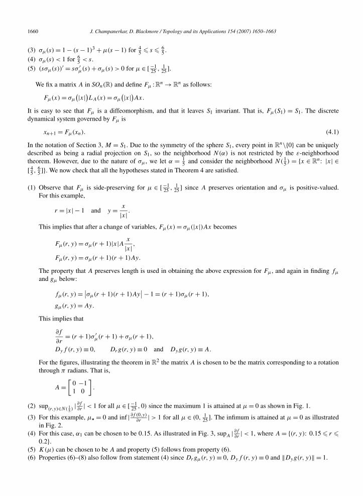
1660 J. Champanerkar, D. Blackmore / Topology and its Applications 154 (2007) 1650–1663
(3) σμ(s) = 1 − (s − 1)3 + μ(s − 1) for 45 � s � 6
5 .(4) σμ(s) < 1 for 6
5 < s.(5) (sσμ(s))′ = sσ ′
μ(s) + σμ(s) > 0 for μ ∈ [−125 , 1
25 ].
We fix a matrix A in SOn(R) and define Fμ : Rn → Rn as follows:
Fμ(x) = σμ
(|x|)LA(x) = σμ
(|x|)Ax.
It is easy to see that Fμ is a diffeomorphism, and that it leaves S1 invariant. That is, Fμ(S1) = S1. The discretedynamical system governed by Fμ is
xn+1 = Fμ(xn). (4.1)
In the notation of Section 3, M = S1. Due to the symmetry of the sphere S1, every point in Rn\{0} can be uniquely
described as being a radial projection on S1, so the neighborhood N(α) is not restricted by the ε-neighborhoodtheorem. However, due to the nature of σμ, we let α = 1
5 and consider the neighborhood N( 15 ) = {x ∈ R
n: |x| ∈[ 4
5 , 65 ]}. We now check that all the hypotheses stated in Theorem 4 are satisfied.
(1) Observe that Fμ is side-preserving for μ ∈ [−125 , 1
25 ] since A preserves orientation and σμ is positive-valued.For this example,
r = |x| − 1 and y = x
|x| .
This implies that after a change of variables, Fμ(x) = σμ(|x|)Ax becomes
Fμ(r, y) = σμ(r + 1)|x|A x
|x| ,Fμ(r, y) = σμ(r + 1)(r + 1)Ay.
The property that A preserves length is used in obtaining the above expression for Fμ, and again in finding fμ
and gμ below:
fμ(r, y) = ∣∣σμ(r + 1)(r + 1)Ay∣∣ − 1 = (r + 1)σμ(r + 1),
gμ(r, y) = Ay.
This implies that
∂f
∂r= (r + 1)σ ′
μ(r + 1) + σμ(r + 1),
Dyf (r, y) ≡ 0, Drg(r, y) ≡ 0 and Dyg(r, y) ≡ A.
For the figures, illustrating the theorem in R2 the matrix A is chosen to be the matrix corresponding to a rotation
through π radians. That is,
A =[
0 −11 0
].
(2) sup(r,y)∈N( 1
5 )| ∂f∂r
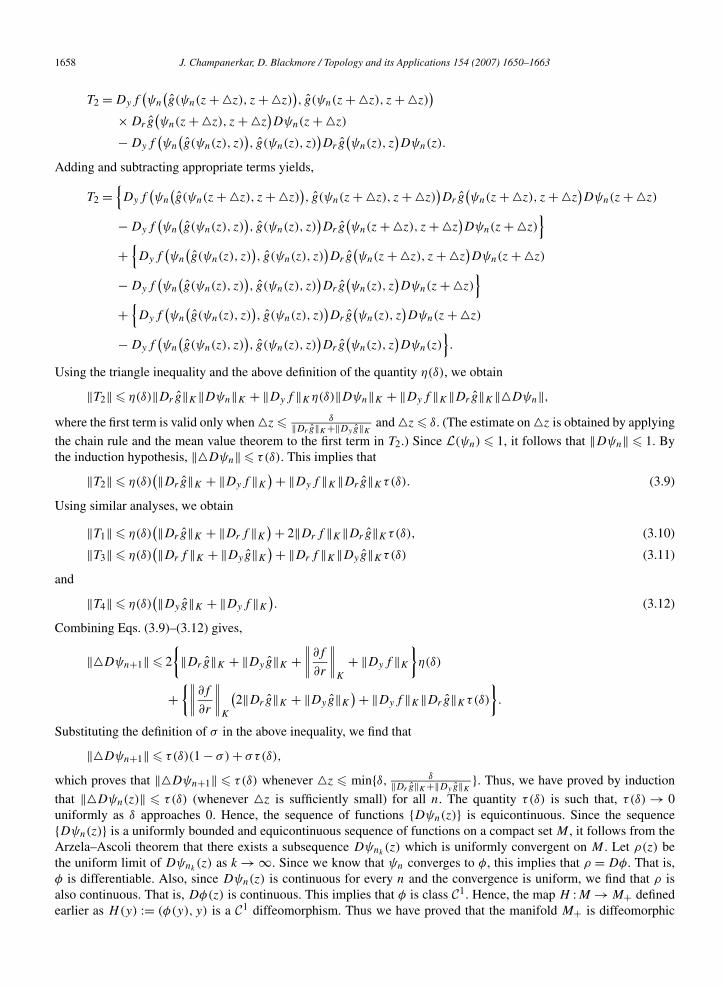
| < 1 for all μ ∈ [−125 ,0) since the maximum 1 is attained at μ = 0 as shown in Fig. 1.
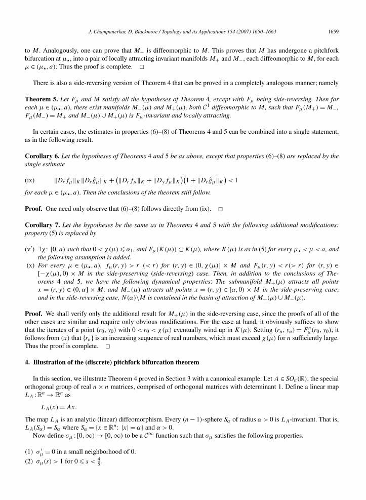
(3) For this example, μ� = 0 and inf | ∂f (0,y)∂r
| > 1 for all μ ∈ (0, 125 ]. The infimum is attained at μ = 0 as illustrated
in Fig. 2.(4) For this case, α1 can be chosen to be 0.15. As illustrated in Fig. 3, supA | ∂f
∂r| < 1, where A = {(r, y): 0.15 � r �
0.2}.(5) K(μ) can be chosen to be A and property (5) follows from property (6).(6) Properties (6)–(8) also follow from statement (4) since Drgμ(r, y) ≡ 0, Dyf (r, y) ≡ 0 and ‖Dyg(r, y)‖ = 1.
J. Champanerkar, D. Blackmore / Topology and its Applications 154 (2007) 1650–1663 1661
Fig. 1. r vs. ∂f∂r
for the canonical example for r ∈ [−0.2,0.2] as μ
increases from −125 to 0.
Fig. 2. Plot of μ vs. ∂f∂r
for the canonical example for r = 0 and
μ ∈ [0, 125 ].
Fig. 3. Plot of r vs. ∂f∂r
for the canonical example for r ∈ [−0.2,0.2]as μ increases from 0 through 1
25 .
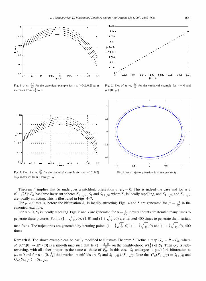
Fig. 4. Any trajectory outside S1 converges to S1.
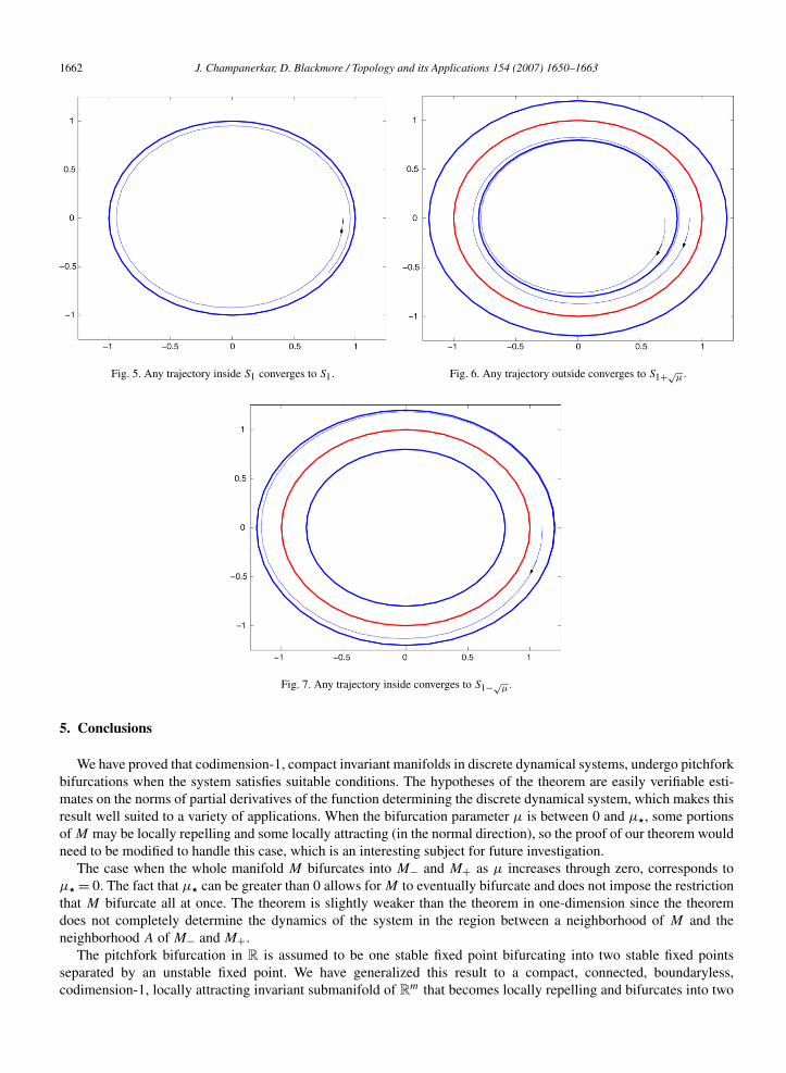
Theorem 4 implies that S1 undergoes a pitchfork bifurcation at μ� = 0. This is indeed the case and for μ ∈(0,1/25]: Fμ has three invariant spheres S1−√
μ, S1 and S1+√μ where S1 is locally repelling, and S1−√
μ and S1+√μ
are locally attracting. This is illustrated in Figs. 4–7.For μ < 0 that is, before the bifurcation S1 is locally attracting. Figs. 4 and 5 are generated for μ = −1
50 in thecanonical example.
For μ > 0, S1 is locally repelling. Figs. 6 and 7 are generated for μ = 150 . Several points are iterated many times to
generate these pictures. Points (1 −√
150 ,0), (1,0) and (1 +
√1
50 ,0) are iterated 400 times to generate the invariant
manifolds. The trajectories are generated by iterating points (1 − 12
√150 ,0), (1 − 3
2
√150 ,0) and (1 + 1
2
√150 ,0), 400
times.
Remark 8. The above example can be easily modified to illustrate Theorem 5. Define a map Gμ = R ◦ Fμ, whereR : Rm\{0} → R
m\{0} is a smooth map such that R(x) = 2−|x||x| on the neighborhood N( 1
5 ) of S1. Then Gμ is side-reversing, with all other properties the same as those of Fμ. In this case, S1 undergoes a pitchfork bifurcation atμ� = 0 and for μ ∈ (0, 1
25 ] the invariant manifolds are S1 and S1−√μ ∪ S1+√
μ. Note that Gμ(S1−√μ) = S1+√
μ andGμ(S1+√
μ) = S1−√μ.
1662 J. Champanerkar, D. Blackmore / Topology and its Applications 154 (2007) 1650–1663
Fig. 5. Any trajectory inside S1 converges to S1. Fig. 6. Any trajectory outside converges to S1+√μ.
Fig. 7. Any trajectory inside converges to S1−√μ.
5. Conclusions
We have proved that codimension-1, compact invariant manifolds in discrete dynamical systems, undergo pitchforkbifurcations when the system satisfies suitable conditions. The hypotheses of the theorem are easily verifiable esti-mates on the norms of partial derivatives of the function determining the discrete dynamical system, which makes thisresult well suited to a variety of applications. When the bifurcation parameter μ is between 0 and μ�, some portionsof M may be locally repelling and some locally attracting (in the normal direction), so the proof of our theorem wouldneed to be modified to handle this case, which is an interesting subject for future investigation.
The case when the whole manifold M bifurcates into M− and M+ as μ increases through zero, corresponds toμ� = 0. The fact that μ� can be greater than 0 allows for M to eventually bifurcate and does not impose the restrictionthat M bifurcate all at once. The theorem is slightly weaker than the theorem in one-dimension since the theoremdoes not completely determine the dynamics of the system in the region between a neighborhood of M and theneighborhood A of M− and M+.
The pitchfork bifurcation in R is assumed to be one stable fixed point bifurcating into two stable fixed pointsseparated by an unstable fixed point. We have generalized this result to a compact, connected, boundaryless,codimension-1, locally attracting invariant submanifold of R
m that becomes locally repelling and bifurcates into two
J. Champanerkar, D. Blackmore / Topology and its Applications 154 (2007) 1650–1663 1663
locally attracting diffeomorphic copies of itself separated by the locally repelling manifold. The techniques we haveused here should enable us to obtain new results on higher dimensional versions of other types of bifurcations such asHopf and saddle-node Hopf bifurcations (see, e.g., [15]). We plan to investigate these and related generalizations inthe future.
Acknowledgements
Part of this paper was taken from the dissertation of the first author submitted to the Faculty of the New JerseyInstitute of Technology in partial fulfillment of the requirements for the degree of Doctor of Philosophy (MathematicalSciences), 2004. The first author wishes to thank the members of her dissertation committee, and especially LeeMosher for his careful reading of the technical details and many helpful suggestions.
References
[1] D. Aronson, G. Chory, G. Hall, R. McGehee, Bifurcations from an invariant circle for two-parameter families of maps of the plane: A com-puter-assisted study, Commun. Math. Phys. 83 (1982) 303–354.
[2] D. Blackmore, J. Champanerkar, C. Wang, A generalized Poincaré–Birkhoff theorem with applications to coaxial vortex ring motion, DiscreteContin. Dyn. Syst. Ser. B 5 (2005) 15–33.
[3] D. Blackmore, J. Chen, J. Perez, M. Savescu, Dynamical properties of discrete Lotka–Volterra equations, Chaos Solitons Fractals 12 (13)(2001) 2553–2568.
[4] H. Broer, G. Huitema, F. Takens, B. Braaksma, Unfoldings and Bifurcations of Quasi-periodic Tori, in: Mem. Amer. Math. Soc., vol. 83,AMS, Providence, RI, 1990, p. 421.
[5] H. Broer, G. Huitema, M. Sevryuk, Quasi-Periodic Motions in Families of Dynamical Systems, Berlin, Springer-Verlag, 1996.[6] H. Broer, H. Osinga, G. Vegter, Algorithms for computing normally hyperbolic invariant manifolds, ZAMP 48 (1997) 480–524.[7] A. Chenciner, Bifurcations de points fixes elliptiques I: Courbes invariantes, Publ. Math. 61 (1985) 67–127.[8] A. Chenciner, Bifurcations de points fixes elliptiques II: Orbites périodique et ensembles de Cantor invariants, Invent. Math. 80 (1985) 81–106.[9] A. Chenciner, Bifurcations de points fixes elliptiques III: Orbites périodique de ‘petites’ périodes et élimination résonnante des couples de
courbes invariantes, Inst. Hautes Études Sci. Publ. Math. 66 (1988) 5–91.[10] P. Glendinning, Non-smooth pitchfork bifurcations, Discrete Contin. Dyn. Syst. Ser. B 4 (2) (2004) 457–464.[11] V. Guillemin, A. Pollack, Differential Topology, Prentice-Hall Inc., Englewood Cliffs, NJ, 1974.[12] P. Hartman, Ordinary Differential Equations, vol. 38, Society for Industrial and Applied Mathematics (SIAM), Philadelphia, PA, 2002.[13] M.W. Hirsch, C.C. Pugh, M. Shub, Invariant Manifolds, Lecture Notes in Mathematics, vol. 583, Springer-Verlag, Berlin, 1977.[14] M. Iwasaki, Y. Nakamura, On the convergence of a solution of the discrete Lotka–Volterra system, Inverse Problems 18 (6) (2002) 1569–1578.[15] B. Krauskopf, B. Oldeman, A planar model system for the saddle-node Hopf bifurcation with global reinjection, Nonlinearity 17 (4) (2004)
1119–1151.[16] B. Krauskopf, H. Osinga, Computing geodesic level sets on global (un)stable manifolds of vector fields, SIAM J. Applied Dynamical Sys-
tems 2 (4) (2003) 546–569.[17] Y. Kuznetsov, Elements of Bifurcation Theory, third ed., Springer-Verlag, New York, 2004.[18] H. Osinga, J. Wiersig, P. Glendinning, U. Feudel, Multistability and nonsmooth bifurcations in the quasiperiodically forced circle map,
Internat. J. Bifur. Chaos Appl. Sci. Engrg. 11 (12) (2001) 3085–3105.[19] L. Perko, Differential Equations and Dynamical Systems, Texts in Applied Mathematics, vol. 7, Springer-Verlag, New York, 2001.[20] S.N. Rasband, Chaotic Dynamics of Nonlinear Systems, John Wiley & Sons Inc. (A Wiley-Interscience Publication), New York, 1990.[21] M. Shub, Global Stability of Dynamical Systems, Springer-Verlag, New York, 1987.[22] R. Sturman, Scaling of intermittent behaviour of a strange nonchaotic attractor, Phys. Lett. A 259 (5) (1999) 355–365.[23] S. Wiggins, Introduction to Applied Nonlinear Dynamical Systems and Chaos, Texts in Applied Mathematics, vol. 2, Springer-Verlag, New
York, 1990.