physics, mathematics and modelingweb.engr.uky.edu/~acfd/lctr-notes634.pdf · introductory lectures...
TRANSCRIPT
INTRODUCTORY
LECTURES on TURBULENCEPhysics, Mathematics and Modeling
J. M. McDonough
Departments of Mechanical Engineering and Mathematics
University of Kentucky
c©2004, 2007

Contents
1 Fundamental Considerations 11.1 Why Study Turbulence? . . . . . . . . . . . . . . . . . . . . . . . . . . . . . . . . . . . . . . 11.2 Some Descriptions of Turbulence . . . . . . . . . . . . . . . . . . . . . . . . . . . . . . . . . 11.3 A Brief History of Turbulence . . . . . . . . . . . . . . . . . . . . . . . . . . . . . . . . . . . 6
1.3.1 General overview . . . . . . . . . . . . . . . . . . . . . . . . . . . . . . . . . . . . . . 61.3.2 Three eras of turbulence studies . . . . . . . . . . . . . . . . . . . . . . . . . . . . . 10
1.4 Definitions, Mathematical Tools, Basic Concepts . . . . . . . . . . . . . . . . . . . . . . . . 111.4.1 Definitions . . . . . . . . . . . . . . . . . . . . . . . . . . . . . . . . . . . . . . . . . 111.4.2 Mathematical tools . . . . . . . . . . . . . . . . . . . . . . . . . . . . . . . . . . . . . 271.4.3 Further basic concepts . . . . . . . . . . . . . . . . . . . . . . . . . . . . . . . . . . . 37
1.5 Summary . . . . . . . . . . . . . . . . . . . . . . . . . . . . . . . . . . . . . . . . . . . . . . 57
2 Statistical Analysis and Modeling of Turbulence 592.1 The Reynolds-Averaged Navier–Stokes Equations . . . . . . . . . . . . . . . . . . . . . . . . 59
2.1.1 Derivation of the RANS equations . . . . . . . . . . . . . . . . . . . . . . . . . . . . 602.1.2 Time-dependent RANS equations . . . . . . . . . . . . . . . . . . . . . . . . . . . . . 632.1.3 Importance of vorticity and vortex stretching to turbulence . . . . . . . . . . . . . . 652.1.4 Some general problems with RANS formulations . . . . . . . . . . . . . . . . . . . . 682.1.5 Reynolds-averaged Navier–Stokes Models . . . . . . . . . . . . . . . . . . . . . . . . 78
2.2 The Kolmogorov Theory of Turbulence . . . . . . . . . . . . . . . . . . . . . . . . . . . . . . 972.2.1 Kolmogorov’s “universality” assumptions . . . . . . . . . . . . . . . . . . . . . . . . 972.2.2 Hypotheses employed by Frisch [80] . . . . . . . . . . . . . . . . . . . . . . . . . . . 982.2.3 Principal results of the K41 theory . . . . . . . . . . . . . . . . . . . . . . . . . . . . 99
2.3 Summary . . . . . . . . . . . . . . . . . . . . . . . . . . . . . . . . . . . . . . . . . . . . . . 104
3 Large-Eddy Simulation and Multi-Scale Methods 1073.1 Large-Eddy Simulation . . . . . . . . . . . . . . . . . . . . . . . . . . . . . . . . . . . . . . . 107
3.1.1 Comparison of DNS, LES and RANS methods . . . . . . . . . . . . . . . . . . . . . 1083.1.2 The LES decomposition . . . . . . . . . . . . . . . . . . . . . . . . . . . . . . . . . . 1103.1.3 Derivation of the LES filtered equations . . . . . . . . . . . . . . . . . . . . . . . . . 1113.1.4 Subgrid-scale models for LES . . . . . . . . . . . . . . . . . . . . . . . . . . . . . . . 1143.1.5 Summary of basic LES methods . . . . . . . . . . . . . . . . . . . . . . . . . . . . . 120
3.2 Dynamical Systems and Multi-Scale Methods . . . . . . . . . . . . . . . . . . . . . . . . . . 1213.2.1 Some basic concepts and tools from dynamical systems theory . . . . . . . . . . . . 1213.2.2 The Navier–Stokes equations as a dynamical system . . . . . . . . . . . . . . . . . . 1323.2.3 Multi-scale methods and alternative approaches to LES . . . . . . . . . . . . . . . . 1343.2.4 Summary of dynamical systems/multi-scale methods . . . . . . . . . . . . . . . . . . 161
3.3 Summary . . . . . . . . . . . . . . . . . . . . . . . . . . . . . . . . . . . . . . . . . . . . . . 162
References 163
i

ii CONTENTS
List of Figures
1.1 da Vinci sketch of turbulent flow. . . . . . . . . . . . . . . . . . . . . . . . . . . . . . . . . . 2
1.2 The Reynolds experiment; (a) laminar flow, (b) early transitional (but still laminar) flow,and (c) turbulence. . . . . . . . . . . . . . . . . . . . . . . . . . . . . . . . . . . . . . . . . . 3
1.3 Movements in the study of turbulence, as described by Chapman and Tobak [1]. . . . . . . 10
1.4 Plots of parts of Reynolds decomposition. . . . . . . . . . . . . . . . . . . . . . . . . . . . . 34
1.5 Turbulence energy wavenumber spectrum. . . . . . . . . . . . . . . . . . . . . . . . . . . . . 48
1.6 Low-pass and high-pass filtered parts of a signal. . . . . . . . . . . . . . . . . . . . . . . . . 49
1.7 Comparison of laminar and turbulent velocity profiles in a duct; (a) laminar, and (b) turbulent. 55
1.8 Law of the wall. . . . . . . . . . . . . . . . . . . . . . . . . . . . . . . . . . . . . . . . . . . . 56
2.1 Multiple time scales for construction of time-dependent RANS equations. . . . . . . . . . . 64
2.2 Loss of information due to averaging; (a) the complete signal, and (b) the time-averagedsignal. . . . . . . . . . . . . . . . . . . . . . . . . . . . . . . . . . . . . . . . . . . . . . . . . 69
2.3 Comparison of various k–ε models for flow over a rib of square cross section. . . . . . . . . . 93
2.4 Drag coefficient vs. Re for flow over a circular cylinder, from experimental data referencedin Tritton [127]. . . . . . . . . . . . . . . . . . . . . . . . . . . . . . . . . . . . . . . . . . . . 100
3.1 Energy spectrum showing cut-off wavenumbers for filtered (kc) and test-filtered (k′c) quantities.115
3.2 Energy spectrum depicting scale similarity. . . . . . . . . . . . . . . . . . . . . . . . . . . . 120
3.3 Time series of a steady solution to an ODE dynamical system. . . . . . . . . . . . . . . . . 122
3.4 Phase portrait of steady attractor. . . . . . . . . . . . . . . . . . . . . . . . . . . . . . . . . 122
3.5 Bifurcation (transition) to convection in Rayleigh–Benard problem; (a) conduction, and (b)convection. . . . . . . . . . . . . . . . . . . . . . . . . . . . . . . . . . . . . . . . . . . . . . 123
3.6 Qualitative bifurcation diagram for Rayleigh–Benard convection. . . . . . . . . . . . . . . . 124
3.7 Time series of (a) periodic and (b) subharmonic solutions to an ODE dynamical system. . . 125
3.8 Comparison of phase portraits of (a) periodic, and (b) subharmonic attractors. . . . . . . . 125
3.9 Subharmonic bifurcation sequence (a) periodic, (b) subharmonic and (c) second subharmonic.126
3.10 Construction of the “1/3” Cantor set. . . . . . . . . . . . . . . . . . . . . . . . . . . . . . . 128
3.11 Geometric representation of construction of a strange attractor. . . . . . . . . . . . . . . . . 129
3.12 Demonstration of scale similarity in Henon map. . . . . . . . . . . . . . . . . . . . . . . . . 131
3.13 (a) Sensitivity to initial conditions in the PMNS equation DDS, and (b) corresponding phaseportrait. . . . . . . . . . . . . . . . . . . . . . . . . . . . . . . . . . . . . . . . . . . . . . . . 132
3.14 Example multi-scale gridding. . . . . . . . . . . . . . . . . . . . . . . . . . . . . . . . . . . . 136
3.15 Example multi-scale gridding. . . . . . . . . . . . . . . . . . . . . . . . . . . . . . . . . . . . 138
3.16 Grid point locations used for second-order structure function averaging in the 3-D uniform-grid case. . . . . . . . . . . . . . . . . . . . . . . . . . . . . . . . . . . . . . . . . . . . . . . 143
3.17 Physical model employed for synthetic-velocity LES of swirling, buoyant plume in an enclosure.144
3.20 Left side is sequence of experimental time series from [58]; right side presents correspondingcomputational time series from the PMNS equation DDS. . . . . . . . . . . . . . . . . . . . 149
iii
iv LIST OF FIGURES
3.21 PMNS plus thermal energy equation βT vs. αT bifurcation diagrams; (a) horizontal velocity,(b) vertical velocity, and (c) temperature. . . . . . . . . . . . . . . . . . . . . . . . . . . . . 150
3.22 Comparison of PMNS plus thermal convection DDS with DNS. . . . . . . . . . . . . . . . . 1513.23 Comparison of PMNS plus thermal convection equations with high-Ra data of Cioni et al.
[191]. . . . . . . . . . . . . . . . . . . . . . . . . . . . . . . . . . . . . . . . . . . . . . . . . . 1523.24 Regime map displaying possible types of time series from the PMNS equation. . . . . . . . 1533.25 Third-order structure function of PMNS time series for homogeneous, isotropic bifurcation
parameters. . . . . . . . . . . . . . . . . . . . . . . . . . . . . . . . . . . . . . . . . . . . . . 1533.26 Second-, fourth- and sixth-order structure functions from PMNS time series for homoge-
neous, isotropic bifurcation parameters. . . . . . . . . . . . . . . . . . . . . . . . . . . . . . 1543.27 PMNS equation 1-D energy spectrum. . . . . . . . . . . . . . . . . . . . . . . . . . . . . . . 155
Chapter 1
Fundamental Considerations
In this chapter we first consider turbulence from a somewhat heuristic viewpoint, in particular discussing theimportance of turbulence as a physical phenomenon and describing the main features of turbulent flow thatare easily recognized. We follow this with an historical overview of the study of turbulence, beginning withits recognition as a distinct phenomenon by da Vinci and jumping to the works of Boussinesq and Reynoldsin the 19th Century, continuing through important 20th Century work of Prandtl, Taylor, Kolmogorov andmany others, and ending with discussion of an interesting paper by Chapman and Tobak [1] from thelate 20th Century. We then provide a final section in which we begin our formal study of turbulence byintroducing a wide range of definitions and important tools and terminology needed for the remainder ofour studies.
1.1 Why Study Turbulence?
The understanding of turbulent behavior in flowing fluids is one of the most intriguing, frustrating—and important—problems in all of classical physics. It is a fact that most fluid flows are turbulent, andat the same time fluids occur, and in many cases represent the dominant physics, on all macroscopicscales throughout the known universe—from the interior of biological cells, to circulatory and respiratorysystems of living creatures, to countless technological devices and household appliances of modern society,to geophysical and astrophysical phenomena including planetary interiors, oceans and atmospheres andstellar physics, and finally to galactic and even supergalactic scales. (It has recently been proposed thatturbulence during the very earliest times following the Big Bang is responsible for the present form ofthe Universe.) And, despite the widespread occurrence of fluid flow, and the ubiquity of turbulence, the“problem of turbulence” remains to this day the last unsolved problem of classical mathematical physics.
The problem of turbulence has been studied by many of the greatest physicists and engineers of the 19th
and 20th Centuries, and yet we do not understand in complete detail how or why turbulence occurs, norcan we predict turbulent behavior with any degree of reliability, even in very simple (from an engineeringperspective) flow situations. Thus, study of turbulence is motivated both by its inherent intellectualchallenge and by the practical utility of a thorough understanding of its nature.
1.2 Some Descriptions of Turbulence
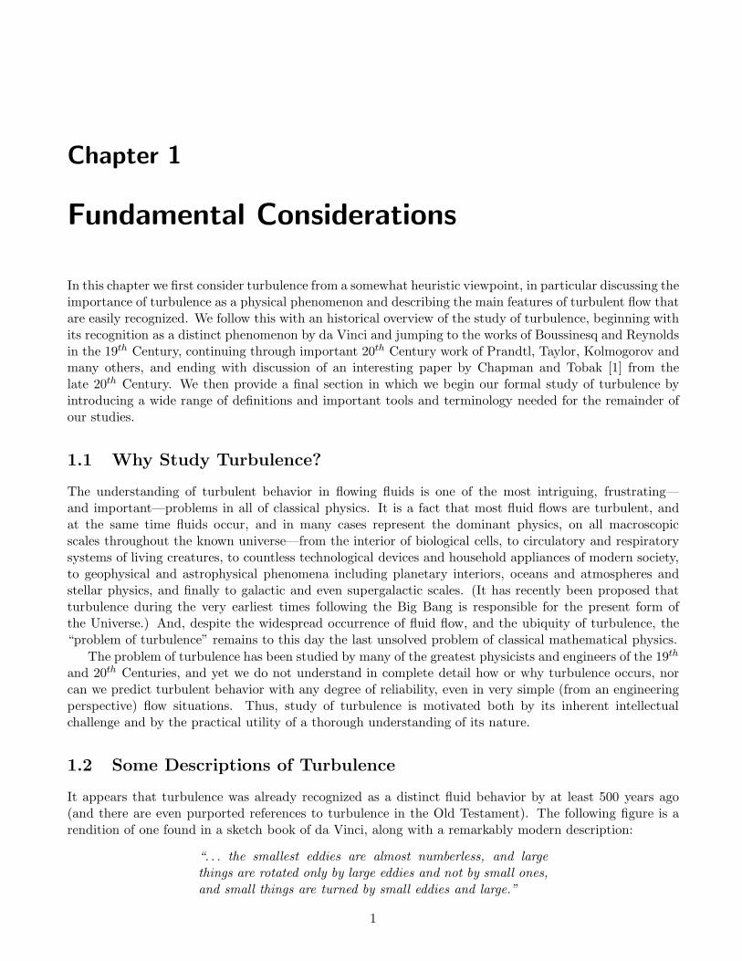
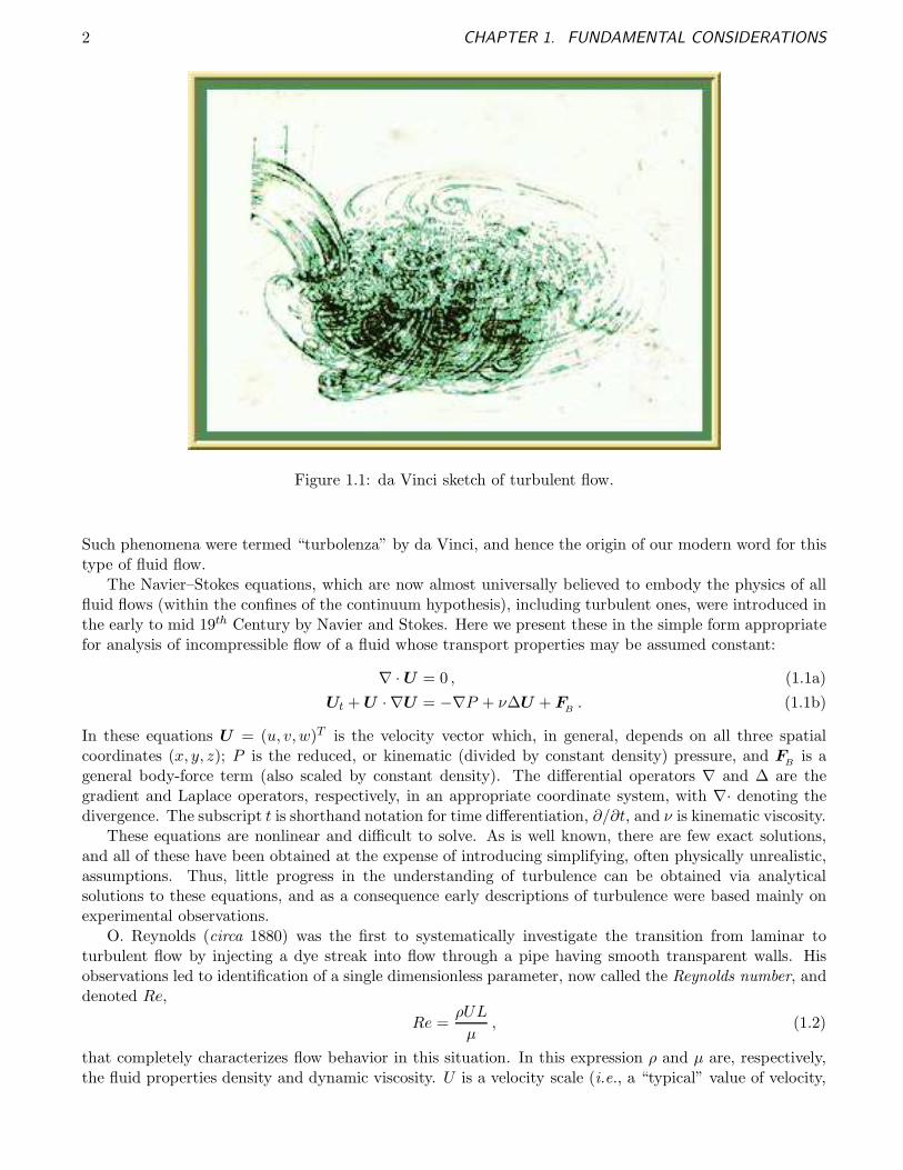
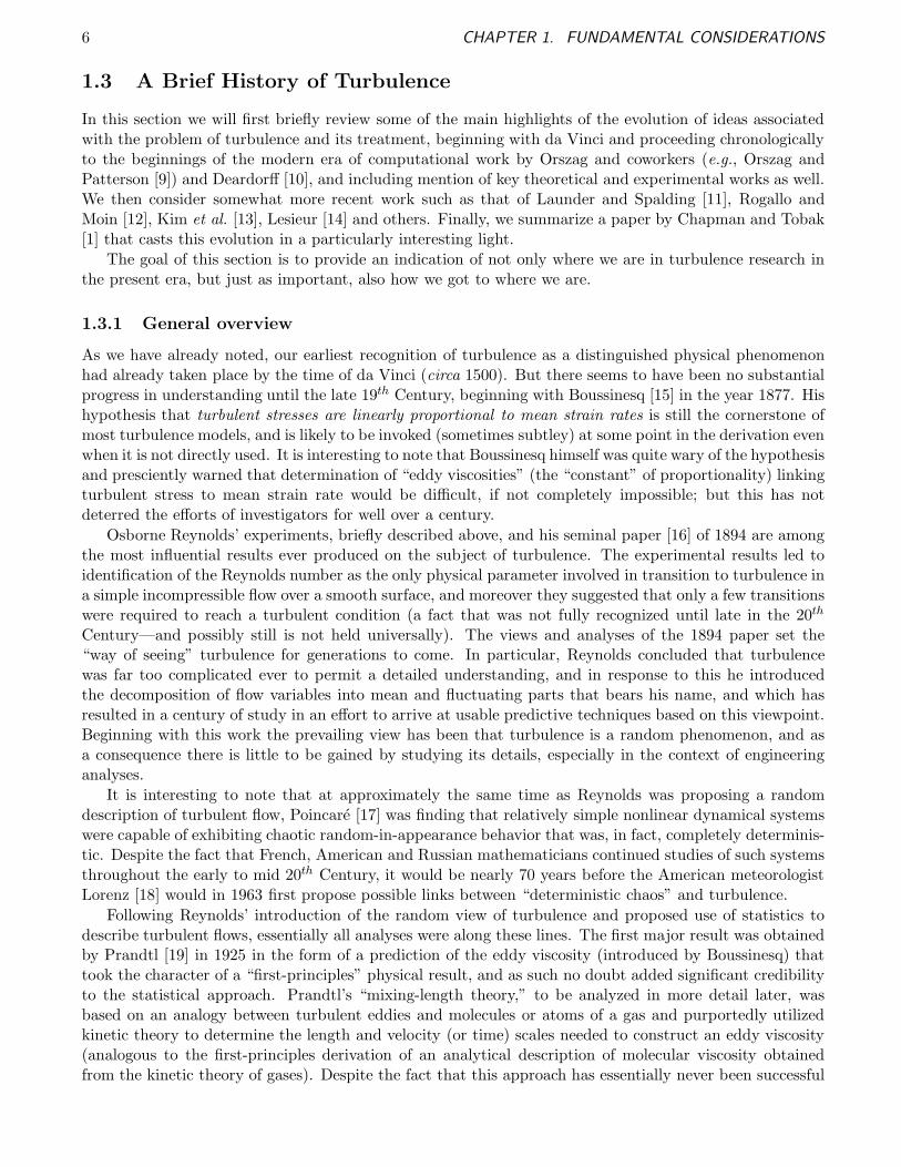
It appears that turbulence was already recognized as a distinct fluid behavior by at least 500 years ago(and there are even purported references to turbulence in the Old Testament). The following figure is arendition of one found in a sketch book of da Vinci, along with a remarkably modern description:
“. . . the smallest eddies are almost numberless, and largethings are rotated only by large eddies and not by small ones,and small things are turned by small eddies and large.”
1
2 CHAPTER 1. FUNDAMENTAL CONSIDERATIONS
Figure 1.1: da Vinci sketch of turbulent flow.
Such phenomena were termed “turbolenza” by da Vinci, and hence the origin of our modern word for thistype of fluid flow.
The Navier–Stokes equations, which are now almost universally believed to embody the physics of allfluid flows (within the confines of the continuum hypothesis), including turbulent ones, were introduced inthe early to mid 19th Century by Navier and Stokes. Here we present these in the simple form appropriatefor analysis of incompressible flow of a fluid whose transport properties may be assumed constant:
∇ · U = 0 , (1.1a)
Ut + U · ∇U = −∇P + ν∆U + FB
. (1.1b)
In these equations U = (u, v,w)T is the velocity vector which, in general, depends on all three spatialcoordinates (x, y, z); P is the reduced, or kinematic (divided by constant density) pressure, and F
Bis a
general body-force term (also scaled by constant density). The differential operators ∇ and ∆ are thegradient and Laplace operators, respectively, in an appropriate coordinate system, with ∇· denoting thedivergence. The subscript t is shorthand notation for time differentiation, ∂/∂t, and ν is kinematic viscosity.
These equations are nonlinear and difficult to solve. As is well known, there are few exact solutions,and all of these have been obtained at the expense of introducing simplifying, often physically unrealistic,assumptions. Thus, little progress in the understanding of turbulence can be obtained via analyticalsolutions to these equations, and as a consequence early descriptions of turbulence were based mainly onexperimental observations.
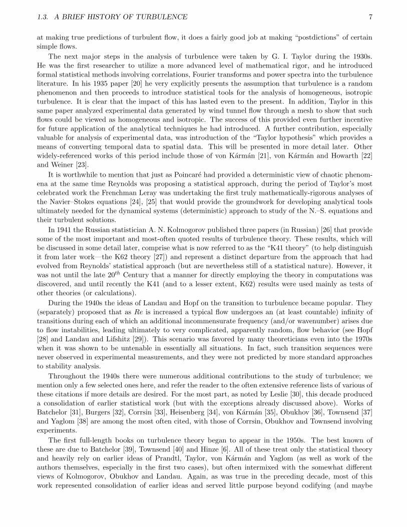
O. Reynolds (circa 1880) was the first to systematically investigate the transition from laminar toturbulent flow by injecting a dye streak into flow through a pipe having smooth transparent walls. Hisobservations led to identification of a single dimensionless parameter, now called the Reynolds number, anddenoted Re,
Re =ρUL
µ, (1.2)
that completely characterizes flow behavior in this situation. In this expression ρ and µ are, respectively,the fluid properties density and dynamic viscosity. U is a velocity scale (i.e., a “typical” value of velocity,
1.2. SOME DESCRIPTIONS OF TURBULENCE 3
say, the average), and L is a typical length scale, e.g., the radius of a pipe through which fluid is flowing.We recall that Re expresses the relative importance of inertial and viscous forces. (The reader may wishto provide a first-principles demonstration of this as a review exercise.)
It is worth noting here that Eqs. (1.1b) can be rescaled and written in terms of Re as follows:
Ut + U · ∇U = −∇P +1
Re∆U + FB , (1.3)
where now pressure will have been scaled by twice the dynamic pressure, 12ρU2, and FB is a dimensionless
body force, often termed the Grashof number in mathematical treatments (see, e.g., Constantin and Foias[2]), but which is more closely related to a Froude number under the present scaling. One can see from(1.3) that in the absence of body forces Re is the only free parameter in the N.–S. equations; hence, settingits value prescibes the solution.
glass pipe
(a)
dye streak
(b)
(c)
instantaneousturbulent streamline
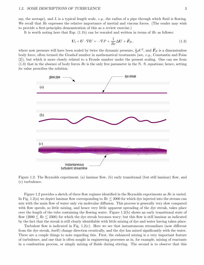
Figure 1.2: The Reynolds experiment; (a) laminar flow, (b) early transitional (but still laminar) flow, and(c) turbulence.
Figure 1.2 provides a sketch of three flow regimes identified in the Reynolds experiments as Re is varied.In Fig. 1.2(a) we depict laminar flow corresponding to Re . 2000 for which dye injected into the stream canmix with the main flow of water only via molecular diffusion. This process is generally very slow comparedwith flow speeds, so little mixing, and hence very little apparent spreading of the dye streak, takes placeover the length of the tube containing the flowing water. Figure 1.2(b) shows an early transitional state offlow (2000 . Re . 2300) for which the dye streak becomes wavy; but this flow is still laminar as indicatedby the fact that the streak is still clearly identifiable with little mixing of dye and water having taken place.
Turbulent flow is indicated in Fig. 1.2(c). Here we see that instantaneous streamlines (now differentfrom the dye streak, itself) change direction erratically, and the dye has mixed significantly with the water.There are a couple things to note regarding this. First, the enhanced mixing is a very important featureof turbulence, and one that is often sought in engineering processes as in, for example, mixing of reactantsin a combustion process, or simply mixing of fluids during stirring. The second is to observe that this
4 CHAPTER 1. FUNDAMENTAL CONSIDERATIONS
mixing ultimately leads to the same end result as molecular diffusion, but on a much faster time scale.Thus, turbulence is often said to “enhance diffusion,” and this viewpoint leads to a particular approach tomodeling as we will see later.
But we should recognize that although the final result of turbulent mixing is the same as that of diffusivemixing, the physical mechanisms are very different. In fact, turbulence arises when molecular diffusioneffects are actually quite small compared with those of macroscopic transport. Here we should recallthe form of Eqs. (1.1b) and note that the second term on the left-hand side corresponds to macroscopictransport (of momentum). These are the “convective” or “advective” terms of the N.–S. equations. Thesecond term on the right-hand side represents molecular diffusion of momentum, as should be clear fromthe fact that its coefficient is a physical transport property (viscosity, in this case) of the fluid and does notdepend on the flow situation (provided we neglect thermal effects), and the differential operator is secondorder. Clearly, if ν is small we should expect advective, nonlinear behavior to be dominant, and this is thecase in a turbulent flow. In contrast to this, if ν is relatively large molecular diffusion will be dominant,and the flow will be laminar. If we recall that ν = µ/ρ, we see that the nonlinear, macroscopic transportcase corresponding to turbulence occurs when the Reynolds number is large.
It is often claimed that there is no good definition of turbulence (see, e.g., Tsinober [3]), and manyresearchers are inclined to forego a formal definition in favor of intuitive characterizations. One of the bestknown of these is due to Richardson [4], in 1922:
Big whorls have little whorls,which feed on their velocity;And little whorls have lesser whorls,And so on to viscosity.
This reflects the physical notion that mechanical energy injected into a fluid is generally on fairly largelength and time scales, but this energy undergoes a “cascade” whereby it is transferred to successivelysmaller scales until it is finally dissipated (converted to thermal energy) on molecular scales. This de-scription underscores a second physical phenomenon associated with turbulence (recall that the first isdiffusion): dissipation of kinetic energy. We comment that this process is also mediated by molecularviscosity, and historically utilization of this has been crucial in modeling efforts as we will outline in moredetail in the sequel.
T. von Karman [5] quotes G. I. Taylor with the following definition of turbulence:
“Turbulence is an irregular motion which in general makes itsappearance in fluids, gaseous or liquid, when they flow pastsolid surfaces or even when neighboring streams of the samefluid flow past or over one another.”
Hinze, in one of the most widely-used texts on turbulence [6], offers yet another definition:
“Turbulent fluid motion is an irregular condition of the flowin which the various quantities show a random variation withtime and space coordinates, so that statistically distinct aver-age values can be discerned.”
It is readily seen that none of these definitions offers any precise characterization of turbulent flow inthe sense of predicting, a priori, on the basis of specific flow conditions, when turbulence will or will notoccur, or what would be its extent and intensity. It seems likely that this lack of precision has at leastto some extent contributed to the inability to solve the turbulence problem: if one does not know whatturbulence is, or under what circumstances it occurs, it is rather unlikely that one can say much of anythingabout it in a quantitative sense.
Chapman and Tobak [1] have described the evolution of our understanding of turbulence in terms ofthree overlapping eras: i) statistical, ii) structural and iii) deterministic. We shall further explore thisviewpoint in the next section, but here we point out that a more precise definition of turbulence is nowpossible within the context of ideas from the deterministic era. Namely,
1.2. SOME DESCRIPTIONS OF TURBULENCE 5
“Turbulence is any chaotic solution to the 3-D Navier–Stokesequations that is sensitive to initial data and which occurs asa result of successive instabilities of laminar flows as a bifur-cation parameter is increased through a succession of values.”
While this definition is still somewhat vague, it contains specific elements that permit detailed exami-nation of flow situations relating to turbulence. In the first place, it specifies equations—the Navier–Stokesequations—whose solutions are to be associated with turbulence. By now it is widely (essentially univer-sally) accepted that the N.–S. equations may exhibit turbulent solutions, while previous definitions havefailed to explicitly acknowledge this. Second, it requires that the fluid behavior be chaotic, i.e., erratic,irregular, as required in earlier definitions, but deterministic and not random (because the N.–S. equationsare deterministic). This is in strong contrast to, especially, Hinze’s definition, but it is overwhelminglysupported by experimental data. Third, we require that turbulence be three dimensional. This is consistentwith the common classical viewpoint (see, e.g., Tennekes and Lumley [7]) where generation of turbulenceis ascribed to vortex stretching which can only occur in 3D as will be considered in more detail below. Butwe comment that chaotic solutions have been obtained from 1-D and 2-D versions of the N.–S. equations,suggesting that chaos is not necessarily turbulence, even when associated with the N.–S. equations.
The modern definition also imposes a requirement of “sensitivity to initial data” which allows one todistinguish highly irregular laminar motion (such as arises in a quasiperiodic flow regime) from actualturbulence. This is lacking in older definitions despite the fact that experimental evidence has alwayssuggested such a requirement. We also comment that this provides a direct link to modern mathematicaltheories of the N.–S. equations in the sense that sensitivity to initial conditions (SIC) is the hallmarkcharacteristic of the “strange attractor” description of turbulence first put forward by Ruelle and Takens[8].
We remark that the notion of loss of stability of the laminar flow regime(s) has both classical andmodern roots. Stability analyses in the context of, mainly, normal mode analysis has been a mainstay instudies of fluid motion for at least a century, and their connections to transition to turbulence were alreadymade in boundary layer studies. The modern contribution is to embed such approaches within bifurcationtheory, thus opening the way to use of many powerful mathematical tools of modern analysis of dynamicalsystems.
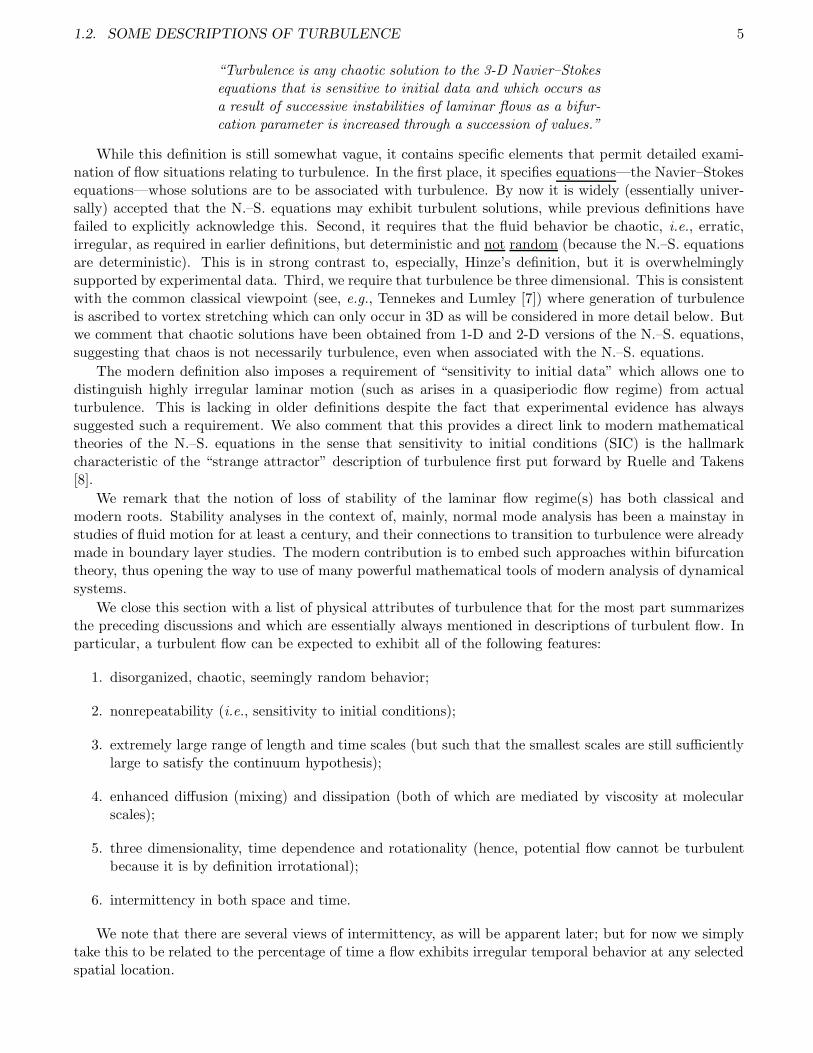
We close this section with a list of physical attributes of turbulence that for the most part summarizesthe preceding discussions and which are essentially always mentioned in descriptions of turbulent flow. Inparticular, a turbulent flow can be expected to exhibit all of the following features:
1. disorganized, chaotic, seemingly random behavior;
2. nonrepeatability (i.e., sensitivity to initial conditions);
3. extremely large range of length and time scales (but such that the smallest scales are still sufficientlylarge to satisfy the continuum hypothesis);
4. enhanced diffusion (mixing) and dissipation (both of which are mediated by viscosity at molecularscales);
5. three dimensionality, time dependence and rotationality (hence, potential flow cannot be turbulentbecause it is by definition irrotational);
6. intermittency in both space and time.
We note that there are several views of intermittency, as will be apparent later; but for now we simplytake this to be related to the percentage of time a flow exhibits irregular temporal behavior at any selectedspatial location.
6 CHAPTER 1. FUNDAMENTAL CONSIDERATIONS
1.3 A Brief History of Turbulence
In this section we will first briefly review some of the main highlights of the evolution of ideas associatedwith the problem of turbulence and its treatment, beginning with da Vinci and proceeding chronologicallyto the beginnings of the modern era of computational work by Orszag and coworkers (e.g., Orszag andPatterson [9]) and Deardorff [10], and including mention of key theoretical and experimental works as well.We then consider somewhat more recent work such as that of Launder and Spalding [11], Rogallo andMoin [12], Kim et al. [13], Lesieur [14] and others. Finally, we summarize a paper by Chapman and Tobak[1] that casts this evolution in a particularly interesting light.
The goal of this section is to provide an indication of not only where we are in turbulence research inthe present era, but just as important, also how we got to where we are.
1.3.1 General overview
As we have already noted, our earliest recognition of turbulence as a distinguished physical phenomenonhad already taken place by the time of da Vinci (circa 1500). But there seems to have been no substantialprogress in understanding until the late 19th Century, beginning with Boussinesq [15] in the year 1877. Hishypothesis that turbulent stresses are linearly proportional to mean strain rates is still the cornerstone ofmost turbulence models, and is likely to be invoked (sometimes subtley) at some point in the derivation evenwhen it is not directly used. It is interesting to note that Boussinesq himself was quite wary of the hypothesisand presciently warned that determination of “eddy viscosities” (the “constant” of proportionality) linkingturbulent stress to mean strain rate would be difficult, if not completely impossible; but this has notdeterred the efforts of investigators for well over a century.
Osborne Reynolds’ experiments, briefly described above, and his seminal paper [16] of 1894 are amongthe most influential results ever produced on the subject of turbulence. The experimental results led toidentification of the Reynolds number as the only physical parameter involved in transition to turbulence ina simple incompressible flow over a smooth surface, and moreover they suggested that only a few transitionswere required to reach a turbulent condition (a fact that was not fully recognized until late in the 20th
Century—and possibly still is not held universally). The views and analyses of the 1894 paper set the“way of seeing” turbulence for generations to come. In particular, Reynolds concluded that turbulencewas far too complicated ever to permit a detailed understanding, and in response to this he introducedthe decomposition of flow variables into mean and fluctuating parts that bears his name, and which hasresulted in a century of study in an effort to arrive at usable predictive techniques based on this viewpoint.Beginning with this work the prevailing view has been that turbulence is a random phenomenon, and asa consequence there is little to be gained by studying its details, especially in the context of engineeringanalyses.
It is interesting to note that at approximately the same time as Reynolds was proposing a randomdescription of turbulent flow, Poincare [17] was finding that relatively simple nonlinear dynamical systemswere capable of exhibiting chaotic random-in-appearance behavior that was, in fact, completely determinis-tic. Despite the fact that French, American and Russian mathematicians continued studies of such systemsthroughout the early to mid 20th Century, it would be nearly 70 years before the American meteorologistLorenz [18] would in 1963 first propose possible links between “deterministic chaos” and turbulence.
Following Reynolds’ introduction of the random view of turbulence and proposed use of statistics todescribe turbulent flows, essentially all analyses were along these lines. The first major result was obtainedby Prandtl [19] in 1925 in the form of a prediction of the eddy viscosity (introduced by Boussinesq) thattook the character of a “first-principles” physical result, and as such no doubt added significant credibilityto the statistical approach. Prandtl’s “mixing-length theory,” to be analyzed in more detail later, wasbased on an analogy between turbulent eddies and molecules or atoms of a gas and purportedly utilizedkinetic theory to determine the length and velocity (or time) scales needed to construct an eddy viscosity(analogous to the first-principles derivation of an analytical description of molecular viscosity obtainedfrom the kinetic theory of gases). Despite the fact that this approach has essentially never been successful
1.3. A BRIEF HISTORY OF TURBULENCE 7
at making true predictions of turbulent flow, it does a fairly good job at making “postdictions” of certainsimple flows.
The next major steps in the analysis of turbulence were taken by G. I. Taylor during the 1930s.He was the first researcher to utilize a more advanced level of mathematical rigor, and he introducedformal statistical methods involving correlations, Fourier transforms and power spectra into the turbulenceliterature. In his 1935 paper [20] he very explicitly presents the assumption that turbulence is a randomphenomenon and then proceeds to introduce statistical tools for the analysis of homogeneous, isotropicturbulence. It is clear that the impact of this has lasted even to the present. In addition, Taylor in thissame paper analyzed experimental data generated by wind tunnel flow through a mesh to show that suchflows could be viewed as homogeneous and isotropic. The success of this provided even further incentivefor future application of the analytical techniques he had introduced. A further contribution, especiallyvaluable for analysis of experimental data, was introduction of the “Taylor hypothesis” which provides ameans of converting temporal data to spatial data. This will be presented in more detail later. Otherwidely-referenced works of this period include those of von Karman [21], von Karman and Howarth [22]and Weiner [23].
It is worthwhile to mention that just as Poincare had provided a deterministic view of chaotic phenom-ena at the same time Reynolds was proposing a statistical approach, during the period of Taylor’s mostcelebrated work the Frenchman Leray was undertaking the first truly mathematically-rigorous analyses ofthe Navier–Stokes equations [24], [25] that would provide the groundwork for developing analytical toolsultimately needed for the dynamical systems (deterministic) approach to study of the N.–S. equations andtheir turbulent solutions.
In 1941 the Russian statistician A. N. Kolmogorov published three papers (in Russian) [26] that providesome of the most important and most-often quoted results of turbulence theory. These results, which willbe discussed in some detail later, comprise what is now referred to as the “K41 theory” (to help distinguishit from later work—the K62 theory [27]) and represent a distinct departure from the approach that hadevolved from Reynolds’ statistical approach (but are nevertheless still of a statistical nature). However, itwas not until the late 20th Century that a manner for directly employing the theory in computations wasdiscovered, and until recently the K41 (and to a lesser extent, K62) results were used mainly as tests ofother theories (or calculations).
During the 1940s the ideas of Landau and Hopf on the transition to turbulence became popular. They(separately) proposed that as Re is increased a typical flow undergoes an (at least countable) infinity oftransitions during each of which an additional incommensurate frequency (and/or wavenumber) arises dueto flow instabilities, leading ultimately to very complicated, apparently random, flow behavior (see Hopf[28] and Landau and Lifshitz [29]). This scenario was favored by many theoreticians even into the 1970swhen it was shown to be untenable in essentially all situations. In fact, such transition sequences werenever observed in experimental measurements, and they were not predicted by more standard approachesto stability analysis.
Throughout the 1940s there were numerous additional contributions to the study of turbulence; wemention only a few selected ones here, and refer the reader to the often extensive reference lists of various ofthese citations if more details are desired. For the most part, as noted by Leslie [30], this decade produceda consolidation of earlier statistical work (but with the exceptions already discussed above). Works ofBatchelor [31], Burgers [32], Corrsin [33], Heisenberg [34], von Karman [35], Obukhov [36], Townsend [37]and Yaglom [38] are among the most often cited, with those of Corrsin, Obukhov and Townsend involvingexperiments.
The first full-length books on turbulence theory began to appear in the 1950s. The best known ofthese are due to Batchelor [39], Townsend [40] and Hinze [6]. All of these treat only the statistical theoryand heavily rely on earlier ideas of Prandtl, Taylor, von Karman and Yaglom (as well as work of theauthors themselves, especially in the first two cases), but often intermixed with the somewhat differentviews of Kolmogorov, Obukhov and Landau. Again, as was true in the preceding decade, most of thiswork represented consolidation of earlier ideas and served little purpose beyond codifying (and maybe
8 CHAPTER 1. FUNDAMENTAL CONSIDERATIONS
mystifying?) these notions so as to provide an aura of infallibility that to the present has been difficult todispel. Moreover, the specific references [39], [40] and [6] presented the problem of turbulence as being sointractable that for several generations few researchers were willing to address it. But it is important tonote that experimental work during this period, and even somewhat earlier, was beginning to cast somedoubt on the consistency, and even the overall validity, of the random view of turbulence. In particular,already as early as the work of Emmons [41] it was clear that a completely random viewpoint was notreally tenable, and by the late 1950s measurement techniques were becoming sufficiently sophisticatedto consistently indicate existence of so-called “coherent structures” contradicting the random view ofturbulence, as already foreseen in a review by Dryden [42] as early as 1948.
By the beginning of the 1960s experimental instrumentation was improving considerably, although theavailable techniques were rather crude by modern standards (laser doppler velocimetry and particle imagevelocimetry were yet to be invented). But the advance that would ultimately lead to sweeping changesin the treatment of turbulence was on the horizon—the digital computer. In 1963 the MIT meteorologistE. Lorenz published a paper [18], based mainly on machine computations, that would eventually leadto a different way to view turbulence. In particular, this work presented a deterministic solution to asimple model of the N.–S. equations which was so temporally erratic that it could not (at the time) bedistinguished from random. Moreover, this solution exhibited the feature of sensitivity to initial conditions(later to be associated with a “strange attractor” in the mathematics literature), and thus essentiallynonrepeatability. Furthermore, solutions to this model contained “structures” in a sense that much laterwould be exploited by McDonough et al. [43], Mukerji et al. [44] and Yang et al. [45] and which might,at least loosely, be associated with the coherent structures being detected by experimentalists—althoughthis was not recognized in 1963. The important point to take from this is that a deterministic solutionto a model of the N.–S. equations (albeit, a very simple one) had been obtained which possessed severalnotable features of physical turbulence.
It is useful to further recognize that throughout the 1960s progress was also being made on the math-ematical understanding of the N.–S. equations, the long-term effects of which would be very significant.Such studies occurred both in the context of basic analysis (i.e., existence, uniqueness and regularity ofsolutions) as exemplified in the landmark book of Ladyzhenskaya [46] and in the field of dynamical systems,where the works of Smale [47] in the U. S. and Arnol’d [48] in the Soviet Union are representative amongmany.
At the same time a new direction was being taken in the attack on the turbulence “closure problem”—the existence of more unknowns than equations in the statistical formulations of turbulence. A numberof new techniques were introduced beginning in the late 1950s with the work of Kraichnan [49], [50] whoutilized mathematical methods from quantum field theory in the analysis of turbulence. These involve useof Fourier representations (both series and transforms), Feynman diagrams and more fundamental (thanN.-S.) equations such as the Liouville and Fokker–Planck equations, to approximate higher moments thatoccur each time an equation for any particular lower moment is constructed. We will not provide detailsof this work herein since for the most part it represents yet another “blind alley” that contributed moreto mystification of the turbulence problem than to its solution. For the interested reader, a quite detailedtreatment, written soon after much of the work was completed, can be found in the book by Leslie [30]published in 1973.
There was also significant progress in experimental studies of turbulence during the decade of the 60s.Efforts were beginning to address quite detailed technical aspects of turbulence such as decay rates ofisotropic turbulence, return to isotropy of homogeneous anisotropic turbulence, details of boundary layertransitions, transition to turbulence in pipes and ducts, effects of turbulence on scalar transport, etc. Theseinclude the works of Comte-Bellot and Corrsin [51] on return to isotropy, Tucker and Reynolds [52] oneffects of plain strain, Wygnanski and Fiedler [53] on boundary layer transition, Gibson [54] on turbulenttransport of passive scalars, and Lumley and Newman [55], also on return to isotropy.
Publication of the seminal paper by Ruelle and Takens [8] in 1971 probably best delineates the beginningof what we will often term a “modern” view of turbulence. In this work it was shown that the N.–S.
1.3. A BRIEF HISTORY OF TURBULENCE 9
equations, viewed as a dynamical system, are capable of producing chaotic solutions exhibiting sensitivity toinitial conditions (SIC) and associated with an abstract mathematical construct called a strange attractor.Furthermore, this paper also presents the sequence of transitions (bifurcations) that a flow will undergo asRe is increased to arrive at this chaotic state, namely,
steady −→ periodic −→ quasiperiodic −→ turbulent
Availability of such a specific prediction motivated much experimentation during the 1970s and 80s todetermine whether this actually occurred. It is to be emphasized that this short sequence of bifurcationsdirectly contradicts the then widely-held Landau–Hopf scenario mentioned earlier.
Indeed, by the late 1970s and early 1980s many experimental results were showing this type of sequence.(In fact, as we mentioned earlier, such short sequences were always seen, but not initially recognized.) But inaddition, other short sequences of transitions to turbulence were also confirmed in laboratory experiments.In particular, the period-doubling subharmonic sequence studied by Feigenbaum [56] as well as sequencesinvolving at least some of the intermittencies proposed by Pomeau and Manneville [57] were observedrepeatedly and consistently. It should be noted further that other transition sequences, usually involving a“phase-locking” phenomenon, were also observed, particularly in flows associated with natural convectionheat transfer (see e.g., Gollub and Benson [58]); but these were still short and in no way suggested validityof the Landau–Hopf view.
Two other aspects of turbulence experimentation in the 70s and 80s are significant. The first of thesewas detailed testing of the Kolmogorov ideas, the outcome of which was general confirmation, but notin complete detail. This general correspondence between theory and experiment, but lack of completeagreement, motivated numerous studies to explain the discrepancies, and similar work continues even tothe present. The second aspect of experimentation during this period involved increasingly more studies offlows exhibiting complex behaviors beyond the isotropic turbulence so heavily emphasized in early work.By the beginning of the 1970s (and even somewhat earlier), attention began to focus on more practical flowssuch as wall-bounded shear flows (especially boundary-layer transition), flow over and behind cylinders andspheres, jets, plumes, etc. During this period results such as those of Blackwelder and Kovasznay [59],Antonia et al. [60], Reynolds and Hussain [61] and the work of Bradshaw and coworkers (e.g., Wood andBradshaw [62]) are well known.
From the standpoint of present-day turbulence investigations probably the most important advances ofthe 1970s and 80s were the computational techniques (and the hardware on which to run them). The firstof these was large-eddy simulation (LES) as proposed by Deardorff [10] in 1970. This was rapidly followedby the first direct numerical simulation (DNS) by Orszag and Patterson [9] in 1972, and introduction ofa wide range of Reynolds-averaged Navier–Stokes (RANS) approaches also beginning around 1972 (seee.g., Launder and Spalding [11] and Launder et al. [63]). In turn, the last of these initiated an enormousmodeling effort that continues to this day (in large part because it has yet to be successful, but at thesame time most other approaches are not yet computationally feasible). We will outline much of this in alater chapter.
It was immediately clear that DNS was not feasible for practical engineering problems (and probablywill not be for at least another 10 to 20 years beyond the present), and in the 70s and 80s this was trueas well for LES. The reviews by Ferziger [64] and Reynolds [65] emphasize this. Thus, great emphasis wasplaced on the RANS approaches despite their many obvious shortcomings that we will note in the sequel.But by the beginning of the 1990s computing power was reaching a level to allow consideration of usingLES for some practical problems if they involved sufficiently simple geometry, and since then a tremendousamount of research has been devoted to this technique. Recent extensive reviews have been provided, forexample, by Lesieur and Metais [66] and Meneveau and Katz [67]. It is fairly clear that for the near futurethis is the method holding the most promise. Indeed, many new approaches are being explored, especiallyfor construction of the required subgrid-scale models. These include the dynamic models of Germano etal. [68] and Piomelli [69], and various forms of “synthetic-velocity” models such as those of Domaradzkiand coworkers (e.g., Domaradzki and Saiki [70]), Kerstein and coworkers (e.g., Echekki et al. [71]) and
10 CHAPTER 1. FUNDAMENTAL CONSIDERATIONS
McDonough and coworkers (e.g., McDonough and Yang [72]). In these lectures we will later outline thebasics of some of these approaches, but will not be able to give complete details. The interested readercan find much of this treated in detail by Sagaut [73].
1.3.2 Three eras of turbulence studies
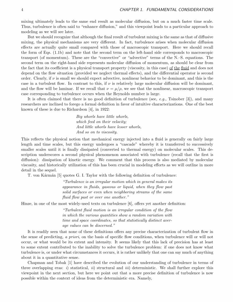
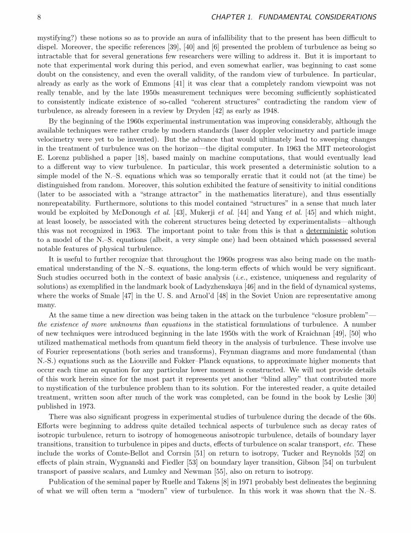
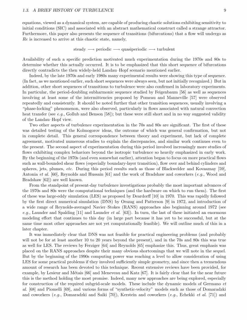
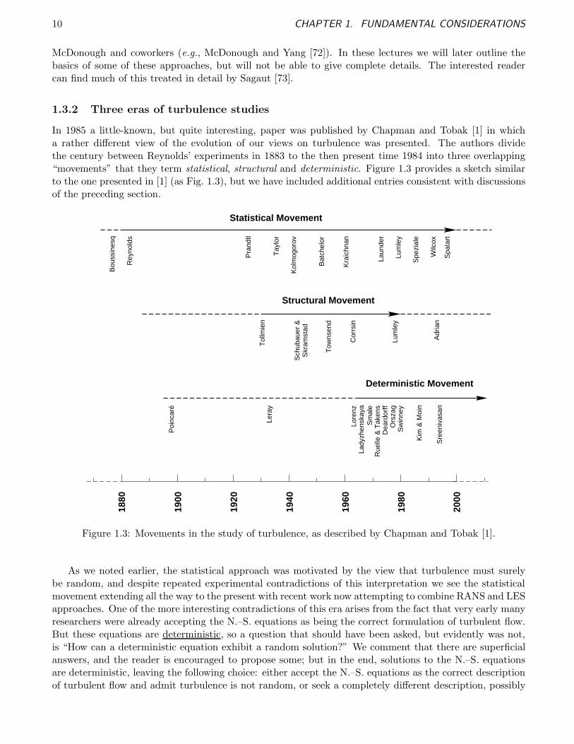
In 1985 a little-known, but quite interesting, paper was published by Chapman and Tobak [1] in whicha rather different view of the evolution of our views on turbulence was presented. The authors dividethe century between Reynolds’ experiments in 1883 to the then present time 1984 into three overlapping“movements” that they term statistical, structural and deterministic. Figure 1.3 provides a sketch similarto the one presented in [1] (as Fig. 1.3), but we have included additional entries consistent with discussionsof the preceding section.
1880
1900
1920
1940
1960
1980
2000
Statistical Movement
Bou
ssin
esq
Rey
nold
s
Pra
ndtl
Tay
lor
Sre
eniv
asan
Kol
mog
orov
Bat
chel
or
Kra
ichn
an
Laun
der
Lum
ley
Spe
zial
e
Wilc
ox
Spa
lart
Sch
ubau
er &
Skr
amst
adStructural Movement
Tol
lmie
n
Tow
nsen
d
Cor
rsin
Lum
ley
Adr
ian
Deterministic Movement
Poi
ncar
é
Lera
y
Lore
nzLa
dyzh
ensk
aya
Sm
ale
Rue
lle &
Tak
ens
Dea
rdor
ffO
rsza
gS
win
ney
Kim
& M
oin
Figure 1.3: Movements in the study of turbulence, as described by Chapman and Tobak [1].
As we noted earlier, the statistical approach was motivated by the view that turbulence must surelybe random, and despite repeated experimental contradictions of this interpretation we see the statisticalmovement extending all the way to the present with recent work now attempting to combine RANS and LESapproaches. One of the more interesting contradictions of this era arises from the fact that very early manyresearchers were already accepting the N.–S. equations as being the correct formulation of turbulent flow.But these equations are deterministic, so a question that should have been asked, but evidently was not,is “How can a deterministic equation exhibit a random solution?” We comment that there are superficialanswers, and the reader is encouraged to propose some; but in the end, solutions to the N.–S. equationsare deterministic, leaving the following choice: either accept the N.–S. equations as the correct descriptionof turbulent flow and admit turbulence is not random, or seek a completely different description, possibly
1.4. DEFINITIONS, MATHEMATICAL TOOLS, BASIC CONCEPTS 11
based on stochastic differential equations. Moreover, if we insist that turbulence is a random phenomenon,then averaging the N.–S. equations as is done in RANS approaches makes little sense—we would be startingwith the wrong equations and yet ending with equations that are not stochastic.
The structural movement is viewed by Chapman and Tobak as having begun possibly with the Schubauerand Skramstad [74] observations of Tollmien–Schlicting waves in 1948; but as we have already noted, eventhe early experiments of Reynolds indicated existence of coherent structures and short bifurcation se-quences. In any case, this movement too persists even to the present, and much research on detecting andanalyzing coherent structures in turbulent flows continues.
In [1] the result of the statistical movement is summarized as “a structureless theory having little powerof conceptualization,” and we add, also little power of prediction at least in part as a consequence of thelack of structure. By way of contrast, the same authors characterize the structural movement as havingproduced “structure without theory.” Because of the massive amounts of data that have arisen duringexperimentation it has been difficult to construct a theory, but in some respects it is not clear that thereactually is much structure either.
Chapman and Tobak show the deterministic movement beginning with the work of Lorenz [18] men-tioned earlier but also note that one could easily include studies as far back as those of Poincare [17].After describing a considerable body of research up to 1984 they conclude that while results of the de-terministic movement are encouraging, as of that date they had not yet provided a successful approachto simulating turbulent flows. (Indeed, even to the present, deterministically-based techniques are oftencriticized for this same reason. DNS is too expensive for practical simulations, and essentially none ofthe efficiently-computed modeling techniques that might be directly linked to the deterministic approachhave proven themselves.) The authors of [1] then conclude the paper by expressing the belief that futuredirections in the study of turbulence will reflect developments of the deterministic movement, but thatthey will undoubtedly incorporate some aspects of both the statistical and structural movements. Wecomment, that in a sense this is proving to be the case. Certainly, LES can be viewed as a product of thedeterministic movement in that the large energy-containing scales are directly computed (as in DNS). Onthe other hand, LES might also be seen in the light of the statistical movement because the subgrid-scale(SGS) models are usually based on a statistical approach. At the same time, there are beginning to beother approaches to SGS model construction that do, in at least an indirect way, incorporate aspects ofthe structural and deterministic movements.
1.4 Definitions, Mathematical Tools, Basic Concepts
In this final section of the chapter we begin our formal studies of turbulence. We will do this by firstintroducing a quite broad range of definitions of various terms that are widely used (and too often notdefined) in turbulence studies, many of which are by now completely taken for granted. Without thesedefinitions a beginning student can find reading even fairly elementary literature rather difficult. Wecontinue in a second subsection with a number of widely-used mathematical constructs including variousforms of averaging, decompositions of flow variables, Fourier series and transforms, etc. Then, in a finalsubsection we introduce some further basic concepts that often arise in the turbulence literature; to someextent this will provide further discussions and applications of terminology appearing in the first twosubsections.
1.4.1 Definitions
In this section we introduce many definitions and terminology to be used throughout these lectures. Werecognize that there is a disadvantage to doing this at the beginning in that nearly all of these will ofnecessity be given out of context. On the other hand, they will all appear in one place, and they will benumbered for easy later reference; thus, this subsection provides a sort of glossary of terms. The reader willrecognize that some of these will have already been used with little or no explanation in earlier sections;
12 CHAPTER 1. FUNDAMENTAL CONSIDERATIONS
so hopefully contents of this section will help to clarify some of the earlier discussions. In general, we willattempt to present ideas, rather than formulas, in the present section, and then provide further elaboration,as needed, in the remaining two subsections of the current section.
We will somewhat arbitrarily classify the terminology presented here in one of three categories, althoughit will be clear that some, if not all, of the terms given could (and sometimes will) appear in one or both ofthe remaining categories. These will be identified as: i) purely statistical, ii) dynamical systems oriented,and iii) physical and computational turbulence.
Purely Statistical
In this section we provide a few definitions of statistical terms often encountered in the study ofturbulence (especially in the classical approach) and elsewhere.
Definition 1.1 (Autocorrelation) Autocorrelation is a function that provides a measure of how well asignal “remembers” where it has been; it is an integral over time (or space) of the value of the signal at agiven time multiplied times a copy with shifted time (or space) argument.
Values of autocorrelation are usually scaled to range between −1 and +1.
Definition 1.2 (Cross correlation) Cross correlation provides a measure of how closely two signals (orfunctions) are related; it is constructed as a scaled inner product of the two functions integrated over adomain (temporal or spatial) of interest.
If two signals are identical, they have a cross correlation equal to unity, and if they everywhere have equalmagnitudes but opposite signs, their cross correlation will be −1. All other possible values lie betweenthese limits.
Definition 1.3 (Ergodicity) Ergodicity implies that time averages and ensemble averages are equivalent.
Note that this is a consequence of the definition, and not actually the definition, itself. (The formaldefinition is rather technical.) The averages mentioned here will be treated in detail in the next section.
Definition 1.4 (Flatness) Flatness requires an equation for formal definition. Here we simply note thatit represents the deviation from Gaussian in the sense that functions having large flatness values are moresharply peaked than are Gaussian distributions, and conversely.
Flatness (sometimes called “kurtosis”) is always greater than zero, and flatness of a Gaussian is exactlythree (3).
Definition 1.5 (Probability density function (pdf)) The probability density function of a random(or otherwise) variable expresses the probability of finding a particular value of the variable over the rangeof definition of the variable.
As with most of the definitions provided here, we will treat this in more detail, and with more formalmathematics, later. The simplest “picture” to remember for a pdf is a histogram scaled so that its area isunity.
Definition 1.6 (Random) A random variable, function, or number is one whose behavior at any latertime (or place) cannot be predicted by knowledge of its behavior at the present time (or place).
It is worth mentioning that the autocorrelation of a random signal decays to zero very rapidly.
Definition 1.7 (Skewness) Skewness is a measure of asymmetry of a function with respect to the origin(or elsewhere).
1.4. DEFINITIONS, MATHEMATICAL TOOLS, BASIC CONCEPTS 13
Skewness can take on both positive and negative values, and that observed in turbulence experiments isusually (but not always) negative. Just as will be the case for flatness, we will later provide a specificformula by means of which to calculate skewness.
Definition 1.8 (Stochastic) A stochastic variable is one whose autocorrelation decays to zero exponen-tially fast.
The notions of randomness and stochasticity are often used interchangeably, but this is not formally correct.Indeed, a deterministic behavior can exhibit stochasticity, but random behavior is always stochastic. Hence,random ⇒ stochastic, but not conversely. A consequence of this is that it makes perfect sense to applystatistical tools in the analysis of deterministic dynamical systems, and this is often done.
Dynamical Systems Oriented
Here we introduce numerous definitions associated with dynamical systems, per se, and also withapplied mathematics of the Navier–Stokes equations.
Definition 1.9 (Attractor) An attractor is a region in phase space to which all trajectories starting fromwithin the basin of attraction are drawn after sufficiently long time, and remain there.
Various of the terms in this definition are, themselves, undefined. This will be taken care of below. Weshould also point out that there are formal technical mathematical definitions for attractor. We will notneed that level of rigor in these lectures.
Definition 1.10 (Basin of attraction) The set of initial data whose trajectories reach the associatedattractor.
It should be mentioned that the basin of attraction is not a trivial notion. Basins can be fractal in nature,implying that changing the value of the initial point by an infinitesimal amount might result in a drasticchange in long-time behavior of the dynamical system. In particular, this is associated with the questionsof uniqueness and stability of solutions to initial value problems.
Definition 1.11 (Bifurcation) A bifurcation (usually termed, simply, a transition in the fluid dynamicsliterature) is a discontinuous qualitative change in system behavior as a (bifurcation) parameter (say, theReynolds number) moves continuously through a critical value.
There are formal mathematical definitions associated with bifurcation, and we will introduce these later,as needed.
Definition 1.12 (Cantor set) The Cantor set is a set formed by starting with the unit interval, and thendiscarding the middle third. This leaves a one-third subinterval on each end. Now we remove the middlethird from each of these, and continue this process ad infinitum.
What remains at the end of this process is a set still containing an uncountable infinity of points, butwhich has zero measure (think length). Moreover, its fractal dimension can be shown to be ∼ 0.62 . . ..
Definition 1.13 (Chaotic) Chaotic is the terminology now used to connote erratic, irregular, disorga-nized, random-in-appearance behavior that is, in fact, deterministic.
Definition 1.14 (Codimension) Codimension refers to the dimension of the space formed by the bifur-cation parameters of a dynamical system.
14 CHAPTER 1. FUNDAMENTAL CONSIDERATIONS
As with most of our definitions in this section, this is not precise, and other definitions are sometimesused. In any case, for our purposes the codimension of a dynamical system is simply its number ofbifurcation parameters. It is worthwhile to note that systems with codimension greater that two arepresently essentially impossible to treat analytically.
Definition 1.15 (Critical value) A value of a bifurcation parameter at which the qualitative behavior ofthe system changes, i.e., a “bifurcation point.”
This corresponds to the situation in which a particular solution to the equations representing a dynamicalsystem is stable for values of the bifurcation parameter that are less than the critical value, and unstablefor those that are greater. As the parameter value passes through the critical one, the original solution(which is still a solution) loses stability and is no longer observed (either physically or computationally)and is replaced with a different stable solution.
Definition 1.16 (Delay map) A delay map is a phase space construction (generally representing anattractor) obtained by plotting the value of a variable against a second, shifted-in-time (delayed), value ofthe same variable as time evolves.
We observe that delay maps are particularly valuable when only incomplete data associated with anattractor are available. In particular, there is a theorem due to Takens [75] that proves that successivetime shifts of data, to each of which is associated an embedding dimension, allows recovery of the topologyof an attractor when only a single variable (out of possibly many) is known completely. The use of thisTakens “embedding theorem” can be especially valuable in treating experimental data where only limitedmeasurements may have been taken.
Definition 1.17 (Deterministic) Deterministic implies predictable, at least for short times. Any behav-ior described by differential and/or algebraic systems possessing no random coefficients or forcings can beexpected to be deterministic.
It is important to note here that predictability may, in fact, be for only a short time. Indeed, deterministicchaos is of precisely this nature—predictable, but not for very long.
Definition 1.18 (Dynamical system) A dynamical system is a mathematical representation, via (usu-ally) differential and/or algebraic equations, of a physical (or otherwise) system evolution starting fromprescribed initial conditions.
Associated with this dynamical system will be a formal solution operator (in the form of a semigroup) thatmaps initial data to results at later times. See Frisch [80] for a precise definition.
Definition 1.19 (Embedding dimension) The embedding dimension is the dimension of a phase spacereconstructed by delays of (usually) a single time series.
An important question, associated with having only a single recording for the behavior of a multi-component dynamical system, is “How large should the embedding dimension be (that is, how many time-delayed variables must be constructed) to guarantee that the topology of the phase space representationis equivalent to that of the original dynamical system?” This is discussed in considerable detail by Takens[75].
Definition 1.20 (Feigenbaum Sequence) A Feigenbaum bifurcation sequence is one associated withperiod-doubling (subharmonic) bifurcations.
1.4. DEFINITIONS, MATHEMATICAL TOOLS, BASIC CONCEPTS 15
We remark that such sequences had been know prior to Feigenbaum’s studies, but previous work did notmatch the detail or depth of his investigations. Primarily through numerical experiments he was able toshow that quadratic maps exibit universal behaviors that can be characterized by two constant determinedby him (see [56]).
Definition 1.21 (Flow) The set of trajectories of a dynamical system generated from all possible initialconditions associated with a particular attractor.
Definition 1.22 (Fractal) An object whose measured linear scales increase with increase in precision ofthe measurements is termed fractal.
We remark that the length of the coastline of Great Britain is often cited as an example of this. Furthermore,for usual fractals as the scale on which measurements (or simply observations) is decreased, the object still“looks the same on every scale.” This is due to what is termed “self similarity.”
Definition 1.23 (Fractal dimension) A fractal dimension is a generally non-integer dimension thatin some way characterizes the structure of a fractal, and which collapses to the usual integer values ofdimension when applied to ordinary, nonfractal objects.
It is worth commenting here that there are numerous ways to compute fractal dimension, and none is par-ticularly easy to carry out. Because a non-integer dimension is considered to be one of the characterizationsof a strange attractor, much effort was expended on arriving at good computational procedures throughoutthe 1980s. However, none of these were completely successful, and other approaches to characterizing astrange attractor are now more often used.
Definition 1.24 (Hilbert space) A Hilbert space is a complete, normed, linear space equipped with aninner product that induces the norm of the space.
The notion of a Hilbert space is incredibly important in the mathematics of the N.–S. equations. In thepresent lectures, however, we will touch on this only lightly.
Definition 1.25 (Inertial manifold) An inertial manifold is a finite-dimensional manifold associatedwith the solution operator (semigroup) of a dynamical system that is (positively) invariant under the semi-group and exponentially attracts all orbits of the dynamical system.
The fact that the inertial manifold of a dynamical system is finite-dimensional implies the possibility ofbeing able to actually compute trajectories on it. If no such object exists, it would be impossible to employDNS to solve the N.–S. equations at high Re.
Definition 1.26 (Intermittency) Intermittency, in the sense of dynamical systems, is one of three phe-nomena associated with switching between nearly steady and chaotic behavior, or between periodic andchaotic behavior.
The detailed mathematical definition of intermittency requires more background than is expected of readersof the present lectures. The interested reader can consult Berge et al. [77] and Frisch [80] and referencestherein.
Definition 1.27 (Invariant sets, manifolds, tori) The term invariant can be applied to any of thesemathematical objects, and others, and refers to the property that the dynamical system (viewed as a semi-group) can map the entire, say manifold of trajectories, back to itself. Then the manifold is said to beinvariant.
16 CHAPTER 1. FUNDAMENTAL CONSIDERATIONS
It is important to note that invariance is not as strong a property as might be thought. In particular, underinvariance alone there is no guarantee that points of a manifold will be mapped back to themselves—onlythat all points of the (invariant) manifold will be mapped back to some point(s) of the manifold by thedynamical system.
Definition 1.28 (Limit cycle) A limit cycle of a dynamical system is a closed trajectory that is followedrepeatedly (cyclicly) for all time.
Definition 1.29 (Lorenz attractor) The Lorenz attractor is the attractor associated with solutions tothe Lorenz [18] equations.
The Lorenz attractor was the first strange attractor to be computed numerically, and when this was carriedout in 1963 the terminology “strange attractor” had not yet appeared in the literature. The importance ofthis attractor is that it was the first to mathematically (albeit, numerically) suggest a connection betweenturbulence and deterministic behavior simply due to the fact that the Lorenz equations comprise a verylow order Galerkin approximation to the N.–S. equations.
Definition 1.30 (Lyapunov exponent) The Lyapunov exponent of a dynamical system provides a time-averaged measure of the rate of divergence of two trajectories that were initially nearby.
We note that positive Lyapunov exponents are generally taken to be a sure sign of a strange attractor(in the case that there is an attractor), and negative ones imply decay of solution behavior to a steadystate. Because of their significance in identifying strange attractors, much effort has been devoted toaccurate, efficient computational techniques for their determination. Some theoretical details can be foundin [77], as well as in many other references, and Wolf et al. [78] provide one of the most widely-usedcomputational procedures. We comment that like fractal dimension calculations, Lyapunov exponentresults are always subject to some uncertainty, and obtaining them tends to be very computationallyintensive. As a consequence, they are not nearly as widely used today as was the case in the 1980s.
Definition 1.31 (Manifold) A manifold is a set whose points can be (at least locally) put into correspon-dence with the points of a Euclidean space of the same dimension.
There are very precise and complicated definitions of manifolds, and many types of manifolds (the interestedreader can consult Wiggins [79] for some details), but here we note that identifying manifolds with smoothsurfaces is not a bad first approximation—although it will fail in the case of a strange attractor. Also,n-dimensional Euclidean space is a manifold for any finite value of n. Thus, in the case n = 3 we havebeen living in a manifold all our lives.
Definition 1.32 (Multifractal) Multifractal refers to a fractal that has multiple fractal character in thesense that scaling to smaller and smaller scales is not self similar as it is in the case of an ordinary fractal.
Definition 1.33 (Orbit) The term orbit refers to a trajectory of a dynamical system that has reached anattractor and thenceforth continues to, in some sense circle around (orbit) the attractor.
The terms orbit and trajectory are obviously closely related, and while they are not completely equivalentthey are often used interchangeably.
Definition 1.34 (Phase lock) Phase lock is a type of periodicity that can arise after a system has reacheda quasiperiodic state (two incommensurate frequencies), and further increases in a bifurcation parameterleads to returning to a two-frequency commensurate state in which the two frequencies are integrally related,and said to be “locked.”
1.4. DEFINITIONS, MATHEMATICAL TOOLS, BASIC CONCEPTS 17
In the physics literature, this condition is often termed resonance, and in some dynamical systems contexts(particularly discrete dynamical systems) the state is called n-periodic because the power spectrum willshow n strong equally-spaced spikes starting with the lower of the two frequencies and ending with thehigher. The n − 1 highest frequencies might be viewed as harmonics of the lowest one, but this is not anaccurate interpretation because of the existence of two frequencies to begin with.
Definition 1.35 (Phase portrait) A phase portrait is a plot of two (or possibly three) components of adynamical system against one another as time evolves.
A simple case of this is the limit cycle often pictured as part of the analysis of stability of periodic solutions.It is also worth noting that the delay maps described above provide an approximation of the phase portrait.
Definition 1.36 (Phase space) Phase space is the region in which a phase portrait (or delay map) isplotted.
Definition 1.37 (PMNS equation) The PMNS equation (poor man’s Navier–Stokes equation) was thename given to a very simple discrete (algebraic) dynamical system by Frisch [80] when arguing that despiteits simplicity, it had many of the aspects of the N.–S. equations.
McDonough and Huang [81], [82] later showed that a somewhat more complicated discrete system could bederived directly from the N.–S. equations and, moreover, that this still relatively simple algebraic systemwas capable of exhibiting essentially any temporal behavior found in the N.–S. partial differential system.
Definition 1.38 (Poincare map) A Poincare map gives the location of the next passing of a trajectorythrough a Poincare section based on the current location of the trajectory.
We note that in general Poincare maps cannot be derived analytically; they must usually be constructednumerically. They provide mainly a qualitative description of overall behavior of a dynamical system;but because they are relatively simple (and easily computed), it has been suggested that they might holdpotential for use in turbulence models.
Definition 1.39 (Poincare section) A Poincare section is a slice (a plane) through the multi-dimensionaltorus containing the trajectories of a dynamical system.
It is not hard to deduce that if the trajectories behave in a chaotic fashion, their points of intersection withany Poincare section will show signs of irregularity as well.
Definition 1.40 (Pomeau–Manneville Sequence) A Pomeau–Manneville bifurcation sequence is onein which chaos arises through a route of behaviors including so-called “intermittencies.” There are at leastthree distinct types of these (see definition, above). More detailed information can be obtained from theearlier cited references, and from [57].
Definition 1.41 (Power spectral density, PSD) The power spectrum of a signal is a function thatgives the power (amplitude) of the signal (usually in decibels, dB) as a function of frequency or wavenumber.
Definition 1.42 (Quasiperiodic) A quasiperiodic signal is one containing two incommensurate (notrationally related) frequencies (or wavenumbers).
As we have indicated earlier, at least in the case of observations and theory associated with N.–S. flows,the quasiperiodic state often occurs as the second bifurcation beyond steady state.
Definition 1.43 (Recurrent) A recurrent behavior in a dynamical system characterizes the fact the thesystem will repeatedly (recurrently) return to any, and all, states of a stationary configuration with aninfinity of such occurrences.
18 CHAPTER 1. FUNDAMENTAL CONSIDERATIONS
We observe that limit cycles are the simplest examples of a recurrent regime, but stationary turbulence istypically also of this nature.
Definition 1.44 (Ruelle–Takens Sequence) The Ruelle and Takens bifurcation sequence consists ofno more than four bifurcations leading to a strange attractor, but the sequence can be as short as three bi-furcations. It typically consists of two Hopf bifurcations from steady behavior (the first to simple periodicity,and the second to quasiperiodicity), followed by a bifurcation to a strange attractor.
We remark that laboratory experiments very early identified modifications of this sequence. In particular,the studies of Gollub and Benson [58] should many different forms of phase-locked behavior; these authorsnote that the specific forms of phase lock and their embeddings within the Ruelle–Takens sequence appearto not be repeatable in laboratory experiments, i.e., they are sensitive to initial conditions.
Definition 1.45 (Self similarity) Self similarity is a property often possessed by fractals leading to astructure that looks the same on all scales.
This property leads to a particular mathematical representation, and one that must be altered in the caseof multifractality.
Definition 1.46 (Sensitivity to initial conditions) Sensitivity to initial conditions (SIC) implies thatthe behavior of a dynamical system can change drastically due to small changes in the initial data.
SIC is one of the main attributes of a strange attractor, and in the context of actual physics is the reasonweather cannot be predicted for more than a few days in advance.
Definition 1.47 (Shell model) Shell models are dynamical systems constructed so as to minimize thenumber of equations (termed “modes” because they typically are obtained via a Galerkin procedure andFourier analysis) needed to reproduce specific aspects of a physical pheneomenon.
Shell models have often been constructed to efficiently mimic behavior of the N.–S. equations, at leastlocally in Fourier space. In this case they are usually designed to reproduce certain symmetries andconservation properties of the N.–S. equations. See Bohr et al. [83] for extensive analyses.
Definition 1.48 (Stable, and unstable, manifold) A stable manifold consists of the set of points inthe trajectories of a dynamical system that approach a specific behavior (say, a fixed point) as t −→ ∞.Corresponding to this is the notion of an unstable manifold which exhibits the same behavior as t −→ −∞.
We note that this definition is lacking precision, but we will not have much specific need for it in the sequel.
Definition 1.49 (Stationary) A dynamical system can be said to exhibit stationary behavior, or station-arity, if it is recurrent and can be assigned a well-defined average with respect to time.
This, like most of our definitions, is rather imprecise and heuristic; but it contains the basic idea: stationarybehavior is, in general, time dependent—it is usually not steady—but it can be viewed as fluctuations aboutsome mean. Frisch [80] provides a precise and quite mathematically-complicated definition, while Tennekesand Lumley [7] use one even simpler than that given here. One should note that steady (time-independent)behavior implies stationarity, but not conversely.
Definition 1.50 (Strange attractor) A strange attractor is an attractor of a dynamical system (seeDef. 1.9 of this section) that can be viewed as having been constructed as the Cartesian product of a smoothmanifold and a Cantor set.
1.4. DEFINITIONS, MATHEMATICAL TOOLS, BASIC CONCEPTS 19
In particular, one might envision a simple strange attractor as being the interior of a two-torus that hashad nearly all of its points removed in a process analogous to the Cantor set construction described inDef. 1.12. A more accurate view comes from recognizing that three main geometric processes occur in thegeneration of a manifold corresponding to a strange attractor: i) shrinking in one or more directions andstretching in one or more directions, ii) rotation, and iii) folding. Indeed, it can be shown that when theseoperations are applied recursively to the flow of a dynamical system, the outcome is a multi-dimensionalversion of a Cantor set. See Alligood et al. [85] and Lanford [86] for more details.
Definition 1.51 (Strong solution) A strong solution (mainly in the context of partial differential equa-tions) is one that satisfies the equations expressed in classical form almost everywhere (a.e.) on the problemdomain of definition.
We remark that the notion of strong solution takes on many different forms, but the important aspect,as the definition implies, is that the solution is sufficiently differentiable to make sense of the differentialequation on all but a set of measure zero in the domain of the problem being considered.
Definition 1.52 (Subharmonic) Subharmonic refers to the appearance of the power spectrum corre-sponding to a signal arising from a period-doubling (or, subharmonic) bifurcation.
The power spectrum will exhibit frequencies at the half frequencies of each of the harmonics of the originalsignal (including, and especially) the fundamental. One can think of this in phase space as arising for anattractor consisting of a simple limit cycle (periodic behavior) after an increase in the bifurcation parameterchanges the dynamics so that the trajectory does not quite return to its starting point after one orbit, andrequires a second orbit to return. This doubles the period and halves the frequency.
Definition 1.53 (Trajectory) A trajectory is the point set in phase space of the path followed by adynamical system starting from a single point of initial data.
Definition 1.54 (Weak solution) A weak solution to a differential equation is one that does not havesufficient differentiability to permit substitution of the solution into the differential equation.
This notion is an extremely important one in the analysis of the N.–S. equations, and it is associatedwith integral forms of these (and other) equations that permit moving derivatives off of formally non-differentiable solutions and onto infinitely-differentiable test functions via integration by parts within alinear functional. In fact, the formal definition of such solutions does not alone admit pointwise evaluation,but practical constructions such as use of Galerkin procedures do yield solutions that can be evaluatedin the usual pointwise sense—but which, nevertheless could have no derivatives. Stakgold [87] provides agood treatment of these ideas.
Physical and Computational Turbulence
In this section we present a wide assortment of terms associated with both the physical and computa-tional aspects of turbulence.
Definition 1.55 (Backscatter) Backscatter is the name often given to the process of transferring turbu-lence kinetic energy from small scales to large ones, or equivalently, from high wavenumbers to low ones.
It is interesting to note that the early theories of turbulence did not include backscatter (despite the factthat Fourier analysis of the N.–S. equations suggests it must occur), and instead viewed transfer of energyas going only from large scales to small.
Definition 1.56 (Boussinesq hypothesis) The Boussinesq hypothesis states that small-scale turbulentstress should be linearly proportional to the mean (large-scale) strain rates.
20 CHAPTER 1. FUNDAMENTAL CONSIDERATIONS
While this idea is an appealing one, since it is somewhat analogous to Newton’s law of viscosity, there isno physical reason why it should hold, and, in fact, in almost all circumstances it does not.
Definition 1.57 (Buffer layer) The buffer layer is the region in wall-bounded flows between the viscoussublayer and the log layer.
Definitions of viscous sublayer and log layer are given below, and as might be expected, they are physicallocations in wall-bounded flows. Intuitively, one should expect that these separate regions (flow behaviors)must be “matched” both physically and mathematically to obtain a well-defined global treatment of sucha flow. The buffer layer is this matching, overlap region.
Definition 1.58 (Closure) Closure refers to finding expressions for terms that arise in averaged andfiltered versions of the N.–S. equations and for which there are no fundamental equations.
The “closure problem” is the outstanding difficulty with any RANS or LES method: there are moreunknowns than there are equations, and this leads to the need for modeling in order to produce a “closed”system of equations.
Definition 1.59 (Coherent structures) Coherent structures are not-very-well-defined behaviors in aturbulent flow, but which are identified as being easy to “see,” may or may not be of fairly large scale, andare somewhat persistent.
As can be seen, there is little about these characterizations that is precise, and this among other thingsmakes looking for coherent structures in experimental data a subjective activity. It is clear that suchstructures exist and are deterministic, but endowing them with a rigorous quantification is difficult.
Definition 1.60 (Cross stress) Cross stresses arise in the formal analysis of LES and consist of productsof resolved- and unresolved-scale quantities.
These arise in LES specifically because a filtered fluctuating quantity is not generally zero. The analogousquantities do not occur (i.e., they are identically zero) in RANS formulations.
Definition 1.61 (Deconvolution method) Deconvolution methods are techniques employed to constructsubgrid-scale models in large-eddy simulation by extracting information from the highest resolved wavenum-ber parts of a solution and using this to infer behavior of the lowest wavenumber unresolved parts.
Definition 1.62 (Defect layer) The defect layer, sometimes simply called the “outer layer,” is the regionof a turbulent boundary layer beyond the log layer (see below), and beginning approximately one-tenth theboundary layer thickness from the wall.
Definition 1.63 (DES) DES is an acronym for detached-eddy simulation. This is a fairly recent devel-opment in turbulence modeling that attempts to improve the efficiency of LES by using RANS approachesin near-wall regions where usual LES would require high resolution to achieve even moderate accuracy.
It should be noted that there are at least two fundamental difficulties with such an approach. The firstis that, as we will see in the next section, the RANS and LES decompositions of dependent variablescorrespond to very different mathematics, so trying to match their results at any particular set of pointsin a flow field is problematic. Second, and associated with this, is the need to determine where this matchshould occur. On the other hand, proponents of this approach argue that formally the equations of LESand RANS are almost identical (if we ignore the point made earlier that RANS must correspond to steadystate), and, even more, the outcome of modeling in either case is increased (numerical) dissipation.
1.4. DEFINITIONS, MATHEMATICAL TOOLS, BASIC CONCEPTS 21
Definition 1.64 (Dissipation range) The dissipation range refers to the length (or, equivalently, wavenum-ber) scales on which the dominant physical phenomenon is viscous dissipation.
The dissipation range corresponds to small length scales (correspondingly, large wavenumbers), and atsuch scales kinetic energy of fluid motion is converted to thermal energy.
Definition 1.65 (DNS) DNS stands for for the numerical procedure direct numerical simulation. Thiscorresponds to solving the Navier–Stokes equations on a digital computer using sufficient resolution tocapture all physically important scales from the largest to the dissipation scales.
It is to be emphasized that no modeling is employed for DNS; there is no closure problem. Thus, theonly problem with this approach is that current computers are not sufficiently large and fast to permit thenecessary resolution if Re is high and/or the problem possesses other physical/geometric complications.
Definition 1.66 (Eddy turnover time) Eddy turnover time is the time taken for a hypothesized turbu-lent eddy to perform one complete 360 rotation.
Definition 1.67 (Eddy viscosity) Eddy viscosity is, formally, the constant of proportionality betweenturbulent (Reynolds) stresses and mean (large-scale) strain rate, analogous to physical viscosity in Newton’slaw of viscosity.
Definition 1.68 (Energy cascade) Energy cascade refers to the transfer of kinetic energy from large,macroscopic scales of motion, where it is presumed to be input to the flow, through successively smallerscales, ending with viscous dissipation and conversion to heat (thermal energy).
The specific physical mechanism proposed for this is interaction of vortices: large vortices break into smallerones that, in turn, break into still smaller ones a la Richardson’s limerick. This view has played a majorrole in development of turbulence models from the beginning, despite the fact that it is not clear suchsuccessions of vortices even exist in many flows. The reader is referred to Tsinober [3] and Kraichnan [88]for a contrary view. We also note here that the energy cascade is often analyzed in terms of dependenceof turbulence kinetic energy on Fourier wavenumbers, and in this context each wavenumber is associatedwith a turbulent eddy size.
Definition 1.69 (Enstrophy) Enstrophy is the L2 norm (squared) of vorticity.
Definition 1.70 (Equilibrium) An equilibrium turbulent flow is one in which production of turbulencekinetic energy is precisely balanced by dissipation of this energy.
It should be noted that this has nothing, per se, to do with thermodynamic equilibrium, or with equilibriumsolutions in the sense of stability analyses.
Definition 1.71 (Friction velocity) Friction velocity is a somewhat artificial construct having dimen-sions of velocity, but defined in terms of the wall shear stress in a wall-bounded flow.
Definition 1.72 (Fully-developed turbulence) Fully-developed turbulence occurs at high Re, and insimple terms can be taken to imply that statistical quantifications of the flow do not change in the flowdirection.
See Frisch [80] for a precise definition.
Definition 1.73 (Galilean invariance) Galilean invariance implies that measured physics must be thesame in any non-accelerating frame of reference. (The term frame invariance is also used.)
22 CHAPTER 1. FUNDAMENTAL CONSIDERATIONS
The importance of this property cannot be overstated. If Galilean invariance did not hold for fluid flow(and, thus, for the N.–S. equations), experimentalists making measurements of identical flow situations atdifferent locations on Earth would record different results.
Definition 1.74 (Helicity) Helicity is the (vector) inner product of the velocity field with its vorticityfield.
We remark that this is not a widely-used concept. On the other hand, Tsinober [3] notes that it “providesa clear indication of direct coupling of large and small scales.” Information of this sort may be valuable inconstruction of advanced turbulence modeling techniques.
Definition 1.75 (Homogeneous turbulence) Homogeneous turbulence is such that statistical proper-ties do not change with spatial translation, i.e., they do not change with position.
It should be noted that it is only the turbulent, fluctuating quantities that are being considered. Inparticular, it is possible to have homogeneous turbulence in a flow field that is nonhomogeneous on largescales. Also, we observe that homogeneity is often viewed with respect to only specified (not necessarilyall) directions.
Definition 1.76 (Implicit large-eddy simulation, ILES) Implicit large-eddy simulation is a relativelynew development in LES studies and consists of solving unfiltered equations; i.e., the N.–S. equations, them-selves, are solved without recourse to any formal turbulence modeling—but on fairly coarse grids.
It is easily recognized that dissipation must be introduced in some manner for this type of approach tosucceed, and in the case of ILES this is done with highly-dissipative discretizations of nonlinear terms inthe N.–S. equations. Thus, the dissipation that would have been produced by a turbulence model in morestandard approaches is obtained directly from the numerical procedures in ILES.
Definition 1.77 (Inertial range) The inertial range, or inertial subrange, is that range of length scales(or wavenumbers) in which viscous effects are essentially negligible.
Definition 1.78 (Integral scale) The integral scale is taken to be an ∼ O(1) to O(10−1), but less thanunity, multiple of the geometric scale of a flow field.
In terms of the energy spectrum, the integral scale is often identified with the wavenumber correspondingto maximum energy. An analogous time scale can also be constructed.
Definition 1.79 (Intermittency) Intermittency (or intermittency factor) is the fraction of total flowtime during which turbulent fluctuations can be observed.
Clearly, this must be viewed locally; the intermittency factor will not be constant throughout a flow field.
Definition 1.80 (Isotropic) Isotropic turbulence exhibits statistics that are independent of rotations andreflections. When this is not the case, the turbulence is anisotropic.
The term local isotropy refers to isotropy only on small scales, identified by their (high) Fourier wavenum-bers. In addition, it should be noted that isotropy implies that statistics for each of the individual fluc-tuating velocity components and their normal direction strains are the same. In turn, because this neednot be true in a homogeneous flow, we see that isotropy is a stronger condition than homogeneity; i.e., ahomogeneous flow may be anisotropic.
1.4. DEFINITIONS, MATHEMATICAL TOOLS, BASIC CONCEPTS 23
Definition 1.81 (k−ε model) The k−ε turbulence models are a class of RANS models for which twoadditional (beyond those for mean flow quantities) partial differential equations must be solved (one forturbulence kinetic energy, k, and one for turbulence kinetic energy dissipation rate, ε) to obtain length andtime scale information needed to construct local (in space) eddy viscosities.
We observe that presently k−ε models are among the most popular for practical engineering problems.They produce results that, basically, are no worse than those obtained from more sophisticated approaches,and they are much less expensive in terms of computer run times.
Definition 1.82 (K41 theory) The K41 theory refers to results published by Kolmogorov in a series ofpapers [26] in 1941.
The K41 theory provides two specific, testable results: the 2/3 law which leads directly to the predictionof a k−5/3 decay rate in the inertial range of the energy spectrum, and the 4/5 law that is the only exact(contains no adjustable constants) result for N.–S. turbulence at high Re. See Frisch [80], and below, formore details.
Definition 1.83 (Kolmogorov scale) Kolmogorov scale is another name for dissipation scales.
These scales were predicted on the basis of dimensional analysis as part of the K41 theory.
Definition 1.84 (Kurtosis) Kurtosis is another name for the statistical quantity flatness; it is actuallyflatness−3.
Definition 1.85 (Landau–Hopf Theory) The Landau–Hopf theory was one of the earlier mathematicaltheories for turbulence where it was hypothesized that turbulence resulted from an infinite sequence ofbifurcations of solutions to the N.–S. equations in each of which a new incommensurate frequency appearedin the solution representation.
It should be noted that this view was at one time very attractive to both mathematicians and turbulencetheorists. It employed easily-understood mathematics to produce a behavior that seemed at least similarto laboratory observations. Experimentalists, however, quickly recognized that there did not appear to beinfinite sequences—but, instead, rather short bifurcation sequences—leading to onset of turbulence. Thisscenario consisting of short sequences was first proven by Ruelle and Takens [8] and was quickly confirmedby numerous experimentalist specifically investigating this issue. We comment further that the work in[8], associating turbulence with a strange attractor, almost completely invalidates the Landau–Hopf theorybecause even though the fluid motion can be extremely complicated in this view, it cannot be sensitive toinitial conditions—a well-known property of both turbulence and strange attractors.
Definition 1.86 (Large scale) Large scale refers to that part of a turbulent flow that carries most of theenergy and corresponds to length scales not extremely smaller than O(1), or correspondingly, wavenumbersthat are ∼ O(1). The small-scale part of the flow is then that part that does not have these properties; inparticular, small scales correspond to high wavenumbers.
Definition 1.87 (Law of the wall) The law of the wall is a semi-empirical expression relating velocityto distance from the wall in a turbulent wall-bounded flow.
There is also a “law of the wake.” Further detailed information on these terms can be found in mostgeneral texts on turbulent flow (e.g., Tennekes and Lumley [7]), and more details will be provided in laterlectures.
Definition 1.88 (Leonard stress) Leonard stresses arises in the analysis of subgrid-scale stresses inLES models as a product of resolved-scale velocity components times resolved-scale velocity components.
24 CHAPTER 1. FUNDAMENTAL CONSIDERATIONS
Observe that these contributions arise due to the fact that a twice-filtered quantity is different from theonce-filtered one for most filters. But it should be noted that this contribution to the SGS stresses can bedirectly computed without modeling.
Definition 1.89 (LES) LES is the acronym for large-eddy simulation.
This form of turbulence calculation lies between DNS and RANS methods, both with respect to form andcost to compute. In particular, in LES the large-scale, energy-carrying motion is directly simulated whilethe small (mainly dissipative) scales are modeled.
Definition 1.90 (Log layer) The log layer is that part of the boundary layer in a wall-bounded flow inwhich a logarithmic semi-empirical result accurately describes the variation of velocity with distance fromthe wall. It corresponds to scaled distances that are relatively far from the wall.
Definition 1.91 (MILES) MILES stands for monotonically integrated large-eddy simulation.
This is a form of LES for which no formal filtering is performed. Instead, a monotone numerical scheme,that introduces artificial viscosity, is applied to discretize the N.–S. equations. This added viscosity isclaimed to be roughly equivalent to that supplied by SGS models in usual LES.
Definition 1.92 (Mixing length) Mixing length is the distance over which a hypothesized turbulent eddyretains its identity.
There are more precise definitions of this quantity (see, e.g., Wilcox [90]) as will be discussed in the sequel.
Definition 1.93 (Moment methods) Moment methods is a generic name sometimes used in referenceto any turbulence computational approach based on RANS equations.
This terminology is widely used in the turbulent combustion literature (see, e.g., Libby [91]).
Definition 1.94 (RANS) RANS is the acronym for Reynolds-Averaged Navier–Stokes approaches toturbulence calculation.
As will be evident in later lectures, RANS approaches are essentially the opposite of DNS, namely, nearlyall scales of the solution must be modeled under a RANS formalism; only (time) mean quantities aredirectly computed.
Definition 1.95 (Realizability) Realizability is the term used to summarize physical constraints thatmust be placed on any turbulence model to avoid direct physical contradictions.
Although it is not obvious, it is possible for RANS models that include a kinetic energy prediction, forexample, to produce negative values of kinetic energy. This is, of course, nonphysical, and any model thatcan yield such a result does not satisfy realizability.
Definition 1.96 (Receptivity) Receptivity is a measure of the tendency of a boundary-layer flow to bedestabilized (starting a transition to turbulence) by freestream disturbances.
Definition 1.97 (Return to isotropy) The phrase return to isotropy is associated with the tendency,of at least the smaller scales of turbulence, to return to a state of approximately equal contributions toturbulence kinetic energy from each velocity component once any source of strain is removed.
Definition 1.98 (RNG) RNG is the acronym for renormalization group.
1.4. DEFINITIONS, MATHEMATICAL TOOLS, BASIC CONCEPTS 25
Renormalization group approaches are adapted from their original use in analysis of phase transitions andhave been intensely studied by McComb [92] and Yahot [93], among others.
Definition 1.99 (Resolved scale) Resolved scale is a name used in LES for the part of the turbulentsolution that is directly computed.
This is often referred to as the large-scale part.
Definition 1.100 (Reynolds analogy) Reynolds analogy provides a relationship between the Stantonnumber and skin friction coefficient for turbulent flows.
Note that the Stanton number is a heat, or mass, transfer coefficient. Thus, the Reynolds analogy providesa direct way to handle turbulence effects on passive scalars once effects on the flow, itself, have beendetermined.
Definition 1.101 (Reynolds stress) Reynolds stresses arise from the averaging procedure used in de-riving the RANS equations. They are the additional unknowns that create the closure problem.
Details of the derivation of the RANS equations will be given in Chap. 2 where modeling of the Reynoldsstresses will also be discussed.
Definition 1.102 (Scale separation) Scale separation implies that the largest scales in a turbulent flowdo not strongly interact with the smallest scales.
Note that the implication of this for modeling is extremely important, viz., models can be constructedindependent of the details of the large-scale flow behavior. See Tsinober [3] for refutation of such ideas.
Definition 1.103 (Scale similarity) Scale similarity is an assumption widely employed in constructionof LES subgrid-scale models, in which it is presumed that the behavior at the lowest wavenumbers of theunresolved part is “similar” to that of the highest wavenumbers of the resolved scale.
This assumption permits at least coarse predictions of behavior on the unresolved scales which may beadequate at low Re, but probably not as Re becomes large.
Definition 1.104 (Second-order closure) Second-order closure refers to a class of RANS models forwhich the second moments (the Reynolds stresses) are directly computed, usually as solutions to partialdifferential equations.
Proponents of RANS models often argue that this approach is far superior because it contains “morephysics” than do, for example, the k−ε methods. But in order to solve the differential equations forthe second moments, the third moments must be modeled; and the models for these are little more thanguesses. In particular, they contain little or no verifiable physics.
Definition 1.105 (Self preservation) Self preservation is a property occurring in flow situations forwhich the turbulence time scales are sufficiently short that as a turbulent disturbance moves downstreamwith the flow it has time to adjust to its new local environment, implying that the turbulence looks the sameat all locations provided it is properly scaled with local variables.
Definition 1.106 (Structure function) Structure functions are averages of differences between turbu-lence quantities measured at different nearby locations in the flow.
Structure functions can be defined for any integer order corresponding to the power to which differences areraised, and are a key part of the Kolmogorov K41 theory. In particular the theory predicts how structurefunctions should scale with distance between measurement points, viz., in the form of a power law.
26 CHAPTER 1. FUNDAMENTAL CONSIDERATIONS
Definition 1.107 (Subgrid-scale (SGS) model) Subgrid-scale models are used in LES to account forthe unresolved part of the solution.
By now there are many different approaches to constructing such models, some of which will be discussedlater.
Definition 1.108 (Subgrid-scale stress) Subgrid-scale stress is the turbulent stress in a LES model thatis analogous to (i.e., arises in the same way as does) Reynolds stress in RANS models.
As hinted in earlier definitions (Defs. 1.60 and 1.88), the SGS stress is more complicated than is theReynolds stress and consists of three contributions: cross stress, Leonard stress, and stress that is analogousto Reynolds stress (and is often termed Reynolds stress) but not identical to it. Despite these complications,most modern SGS stress models treat the entire stress in a single model without decomposing it and treatingdifferent components separately as was once done.
Definition 1.109 (Synthetic-velocity model) Synthetic-velocity models employ direct modeling of theSGS velocities rather than modeling the stresses.
There are several variants of this approach, and it is believed by its proponents that more physics of thesub-grid scales is captured in this way. In particular, among other things this approach permits directaccount of SGS interactions between turbulence and other physics, e.g., chemical kinetics, which is notpossible with usual LES SGS models, or with RANS models. See References [70], [71] and [72] for moreinformation on this approach.
Definition 1.110 (Taylor’s hypothesis) The Taylor’s (frozen-flow) hypothesis states that in a turbulentflow for which the magnitude of the fluctuations is not too great, it is possible to deduce spatial turbulencequantities from time series measured at a single point in the flow.
Definition 1.111 (Taylor microscale) The Taylor microscale corresponds to length scales between theintegral scale and the dissipation scale.
From this description we see that the Taylor microscale length should be of approximately the same orderof magnitude as length scales corresponding to the inertial subrange of the energy spectrum.
Definition 1.112 (Transition) Transition refers to a change from one qualitative state of flow to an-other, and in particular in the context of turbulence studies, the transitions from laminar to turbulentflow.
Use of the term transition is essentially interchangeable with bifurcation from the dynamical systems view.
Definition 1.113 (Turbulence kinetic energy) Turbulence kinetic energy is the kinetic energy calcu-lated with turbulent fluctuating velocities.
It will be clear when we discuss various forms of decomposition of flow variables that exactly what is meantby “turbulent fluctuation” will depend somewhat on the particular decomposition being considered; butin the absence of any specific mention of the decomposition, use of fluctuating velocities from a RANSdecomposition will be assumed.
Definition 1.114 (Turbulence energy dissipation rate) Turbulence energy dissipation rate is the rateat which turbulence energy is being converted to thermal energy by viscous effects on small scales.
Definition 1.115 (URANS) URANS stands for usteady Reynolds-averaged Navier–Stokes.
1.4. DEFINITIONS, MATHEMATICAL TOOLS, BASIC CONCEPTS 27
This is a currently-popular approach to obtaining time-dependent turbulent solutions rather inexpensively;but the approach is inconsistent with the mathematics of constructing the RANS equations, and as can bereasonably expected in such a case, computed results have not been reliable—even qualitatively.
Definition 1.116 (Viscous sublayer) Viscous sublayer is the name given to a very thin layer of fluidimmediately adjacent to the wall in a wall-bounded turbulent flow.
The terminology arises from the fact that the viscous terms are dominant in the N.–S. equations for theconditions of such regions. This layer is sometimes mistakenly termed the “laminar” sublayer, but as notedin [7], this is not correct because there are turbulent fluctuations within this region.
Definition 1.117 (VLES) VLES is the acronym for very large-eddy simulation.
This corresponds to a coarse-grid LES and now is viewed as being equivalent to URANS. But it will beevident when decompositions are studied in the next section that this is not really the case. Moreover,VLES has a potential for good accuracy, at least in a qualitative sense, if accurate SGS models can bedeveloped.
Definition 1.118 (Vortex stretching) Vortex stretching refers to a physical phenomenon involving de-formation of vortices, and which only occurs in three space dimensions.
Vortex stretching is often, in classical turbulence analyses, shown to directly give rise to the Reynoldsstresses (see [7]), and since it can occur only in 3-D it is often argued that there can be no 2-D turbulence.While the conclusion is correct (for other reasons), the entire notion of vortex stretching, per se, is difficultto justify simply because we do not know whether there are any vortices to be stretched at any particularlocation at a given time. On the other hand, vorticity (as a flow property) exists throughout a flow field,and analyses involving “vortex stretching” actually only make use of vorticity. See Ref. [3] for more details.
Definition 1.119 (zero-, one-, two-equation models) Zero-, one-, two-equation models refer to thenumber of partial differential equations needed (beyond the equations for mean quantities) to complete aRANS model.
Zero-equation models are strictly algebraic, one-equation models involve a single additional partial differ-ential equation (PDE), usually providing a length scale. The k−ε model described earlier in Def. 1.81 isthe most widely used two-equation model.
1.4.2 Mathematical tools
In this section we present an assortment of mathematical tools that are often used in the study of turbulence;we will use most, if not all, of these in the sequel. In some cases the discussions provided here will includefurther elaboration on definitions presented in the preceding subsection, and in particular, equations willnow usually be given. We begin with an introduction to Hilbert spaces because these provide a frameworkinto which essentially everything else we do can be cast. This will include definition and discussion ofFourier series and transforms. We next consider forms of averaging and other statistical quantities, andcontinue on with a discussion of decomposition of flow variables. Finally, we introduce the Cartesian tensornotation that is so widely used in classical treatments of turbulence.
Introduction to Hilbert Spaces
Because Hilbert spaces play a crucial role in the modern analysis of the N.–S. equations, and suchanalyses have contributed significantly to the understanding of turbulence and its simulation within thedeterministic framework, we will provide a brief, pedestrian introduction to this important area of applied
28 CHAPTER 1. FUNDAMENTAL CONSIDERATIONS
mathematics that we hope will be sufficient for the present lectures. We first recall Def. 1.24 of a Hilbertspace from the preceding section: a complete, normed, linear space equipped with an inner product thatinduces the norm of the space. We assume familiarity with the notions of norm and linearity, and proceedto a discussion of inner product. Once this is available we will consider Fourier representations of functions.Such representations are important in both analytical and computational studies of the N.–S. equations,and thus for turbulence.
Inner product. The inner product of two functions is given in the following definition.
Definition 1.120 Let u and v be elements of the Hilbert space L2(Ω), Ω ⊆ Rd , d < ∞. Then the innerproduct of u and v is defined as
〈u, v〉 ≡
∫
Ωu(x)v(x) dx . (1.4)
This provides a generalization to infinite-dimensional function spaces of the usual finite-dimensional “dot”product of two vectors, and at the same time is a special case of the scalar product defined on more generalfunction spaces.
It is clear from the definition that
〈u, u〉 =
∫
Ωu(x)u(x) dx =
∫
Ωu2(x) dx ≡ ‖u‖2
L2,
where we are taking u to be real. We see that, as required by the definition of a Hilbert space, the innerproduct induces a norm on the space. We note that any function u is in the space of functions L2(Ω),the canonical Hilbert space, if ‖u‖
L2< ∞. Furthermore, we observe that the notation being used here for
emphasis and clarity is not standard in the context of analysis of the N.–S. equations. In particular, theL2 norm is often denoted in the same way as is the absolute value function and complex modulus, viz.,| · |. We will sometimes use this notation in the sequel.
There is a well-known theorem that further relates the inner product to the L2 norm:
Theorem 1.1 (Cauchy–Schwarz) Let u, v ∈ L2(Ω). Then
〈u, v〉 ≤ ‖u‖L2‖v‖
L2. (1.5)
The proof of this theorem is elementary and can be found, for example, in Stakgold [87].With this information in hand, we are now prepared to consider Fourier series representations of
functions in L2.
Fourier series. We begin with a somewhat informal statement of the result that justifies use of Fourierseries, the Riesz representation theorem (or, in the form we present, sometimes referred to as the Riesz–Fischer theorem), and then discuss some properties of Fourier series.
Theorem 1.2 (Riesz representation) Any function f ∈ L2(Ω) , Ω ⊂ Rd , d < ∞, can be expressed inthe form of a Fourier series,
f(x) =
∞∑
k=−∞
akϕk(x) , (1.6)
with wavevectors k ≡ (k1, . . . , kd)T , and ϕk being a complete (in L2), orthonormal basis. The aks are
the Fourier coefficients.
In particular, for any f ∈ L2, the aks exist, are uniquely defined, and decay to zero sufficiently fast withincreasing |k| to guarantee convergence of the series in a particular sense.
The aks are calculated using the inner product defined above:
ak ≡
∫
Ωf(x)ϕk(x) dx , (1.7)
1.4. DEFINITIONS, MATHEMATICAL TOOLS, BASIC CONCEPTS 29
which by the Cauchy–Schwarz inequality is guaranteed to exist for f ∈ L2 and ϕk no less smooth thanrequired for inclusion in L2. Usually, the ϕks are much smoother, typically being eigenfunctions of aSturm–Liouville problem (see, e.g., [87]) such as sines and cosines, and complex exponentials. Moreover,we note that completeness of the ϕks in L2(Ω) implies that they will be sufficient to construct any functionin L2(Ω).
We comment that what we have called the Riesz representation theorem is actually a special caseof that theorem, i.e., a corollary; the complete theorem is far more general. Furthermore, we note thatconvergence of the series in Eq. (1.6) can be deduced directly from the Parseval identity which we nowstate.
Theorem 1.3 (Parseval identity) Let f ∈ L2(Ω), and let ϕk(x) be a complete orthonormal basis withrespect to L2(Ω). Then ∫
Ω|f(x)|2 dx =
∑
k
|ak|2 . (1.8)
Clearly, since f ∈ L2(Ω), the integral on the left-hand side exists, so the summation on the right-hand sideconverges, implying that the Fourier representation (1.6) converges to f in the L2 norm. That is,
∫
Ω
∣∣∣∣∣f −N∑
k
akϕk
∣∣∣∣∣
2
dx −→ 0
as N → ∞. We leave proof of this as an exercise for the reader.There are several key points to be made regarding the Fourier representation introduced here. First, we
have at no time assumed the function f to be periodic. Although it may well be that the ϕks are periodic,this does not imply that f must also be because we are requiring convergence only in L2. Obviously, afinite sum of akϕk would be periodic if this were true of the ϕks, but this does not generally hold for aninfinite sum. (It is a myth, and a badly misleading and incorrect one, that only periodic functions haveFourier series expansions.) It should also be mentioned that due to details of the Lebesgue integral, it ispossible that the series does not converge at all at (at least) a countable number of points x ∈ Ω (but thisdoes not matter in the sense of L2 convergence).
Finally, if we consider a function that also depends on time, say u(x, t), then the corresponding Fourierrepresentation is
u(x, t) =
∞∑
k=−∞
ak(t)ϕk(x) , (1.9)
with
ak(t) ≡
∫
Ωu(x, t)ϕk(x) dx . (1.10)
In particular, we note that the Fourier coefficients are now time dependent, functions and the representationEq. (1.9) is reminiscent of “separation of variables” from elementary PDE analysis (see, e.g., Berg andMcGregor [95]). Indeed, Eq. (1.9) in some sense provides both a generalization and a justification of thissimple solution technique.
Fourier transforms. Because such a large body of analysis of the N.–S. equations has beenperformed using Fourier transforms, for the sake of completeness, we briefly describe these here. Butwe note that these apply to what is often a different type of function space than present knowledgeof the N.–S. equations would suggest is appropriate (see Foias et al. [89] for more details). Thusit is doubtful that much is to be gained from an exhaustive study, and we will simply provide thedefinition and a few comments.
Definition 1.121 (Fourier transform) Let f ∈ L2(Rd). Then the Fourier transform of f is
F(f)(ω) =
∫
Rd
f(x)e−2πiω·x dx . (1.11)
30 CHAPTER 1. FUNDAMENTAL CONSIDERATIONS
There is, of course, an inverse Fourier transform defined (with appropriate normalization) anddenoted by F−1 so that
F−1(Ff(ω
)(x) = f(x) .
We remark that Fourier transforms have been widely used in the renormalization group (RNG)analyses of N.–S. turbulence by e.g., McComb [92] and Yahot and Orszag [93]. The latter of thesehas served as the starting point for the once highly-touted RNG turbulence models now available inmany commercial CFD codes. But there are fundamental flaws in the analysis presented in [93], asis well known, and results presented by Freitas [94] show that RNG turbulence models are “unstableto implementation details.” That is, two different codes of the same model can produce drasticallydifferent results when applied to the same problem. We thus do not recommend use of such anapproach to turbulence modeling.
Forms of Averaging and Filtering, and Other Statistical Quantities
Both classical (statistical) and modern (deterministic) approaches to the analysis of turbulencegenerally must employ averaging or filtering at some level. Here, we present the various possiblemethods: temporal, spatial and ensemble averaging, and spatial filtering. We then discuss variousother mathematical tools of a, mainly, statistical nature.
Time average. Let u(x, t) be an integrable function with respect to t for t → ∞ and defined forany desired x ∈ Ω ⊂ Rd , d = 1, 2, 3. Then the time average of u at the point x is defined as
u(x) ≡ limT→∞
1
T
∫ T
0
u(x, t) dt . (1.12)
We note that the lower limit of integration is arbitrary and may be shifted as needed. It is clearthat the average can no longer be a function of time, and it follows that all time derivatives of u areidentically zero. We comment that this is often (usually!) ignored in modern treatments of RANSmodeling (see below, and Def. 1.115), but without the formal limit taken in Eq. (1.12), the averageis not well defined, as emphasized, e.g., by Tennekes and Lumley [7].
Spatial average. Let Ω ⊂ Rd , d = 1, 2, 3 with u(x, t) integrable on Ω at any desired time t. Thenthe spatial average of u at time t is
u(t) ≡1
VΩ
∫
Ω
u(x, t) dx , (1.13)
where VΩ denotes the “volume” of Ω. Clearly this is merely the length of an interval when d = 1,and an area when d = 2. We remark that the “ ˜ ” notation will also be used for formal filtering(see below) which when applied spatially, as is usually done in the context of turbulence analysesassociated with LES, represents a straightforward generalization of (1.13).
Ensemble average. Letu(i)(x, t)
N
i=1be a sequence of realizations of a function u(x, t) defined
for x ∈ Ω ⊂ Rd and t ∈ [0, tf ]. Then the ensemble average of u is defined as
〈u(x, t)〉 ≡1
N
N∑
i=1
u(i)(x, t) . (1.14)
Formally one can consider taking the limit N → ∞, but this clearly imposes additional mathe-
matical difficulties and requirements on the sequenceu(i)(x, t)
N
i=1; moreover, in practice—in the
context of either experiments or numerical simulations—N would necessarily be finite. Nevertheless,
1.4. DEFINITIONS, MATHEMATICAL TOOLS, BASIC CONCEPTS 31
there still is a convergence question, namely, “How large must N be before 〈u〉 no longer changessignificantly with increasing N?” Practical experience has shown that such convergence occurs veryslowly, making use of ensemble averages difficult in either experimental or computational contexts.On the other hand, observe that an ensemble-averaged variable is still a function of both x and t,despite the averaging—an often desirable property.
We also mention that the angular-bracket notation, 〈 · 〉, will sometimes be used later to denotea generic averaging process that might be any one of the above forms.
Spatial filtering. For any function u(x, t) in a Hilbert space we define the spatially-filtered functionu(x, t) over a domain Ω as
u(x, t) ≡1
VΩ
∫
Ω
u(ξ, t)G(x|ξ) dξ , (1.15)
where G(x|ξ) is the kernel of the filter, presumed to be at least in L2(Ω). Ω and VΩ are defined asin the case of spatial averaging (corresponding to G ≡ 1), but we observe that in normal usage thefunctions employed for G decay rapidly near the boundaries of subdomains of Ω. As a consequence,in contrast to the spatially-averaged case which is usually global (at least in specific directions), thefiltered function is now local and still dependents on both x and t, just as is the case for ensembleaveraging. We note that an analogous definition holds for temporal filtering. This is seldom usedin turbulence modeling but is widely used in the context of experimental data analysis.
Autocorrelation. Here we provide more details associated with Def. 1.1. Let u(x, t) ∈ L2(0, tf)be stationary with respect to t and bounded for each x ⊂ Rd. Then we define the autocorrelationcoefficient of u at the point x to be
ca(x, τ) ≡〈u(x, t), u(x, t + τ)〉
‖u‖2L2
(1.16)
for each increment τ < tf . Clearly, by the Schwarz inequality, ca(x, τ) takes on values on theinterval [−1, 1].
We remark that it is possible to also define autocorrelation in terms of spatial variables inan analogous fashion. We leave this as an exercise for the reader. Also observe, as discussed inconsiderable detail in [7], that the autocorrelation coefficient leads to an integral time scale T definedas
T ≡
∫ ∞
0
ca(τ) dτ . (1.17)
It should be noted that the infinite upper limit in the integral is formal. The integral time scale isa measure of how long turbulent fluctuations remain correlated, and in practice is taken to be somefraction (∼ 0.5, or less) of the time to the first zero of ca. Hence, T > 0 always holds.
Cross correlation. Analogous to the above, for two stationary functions u(x, t), v(x, t) ∈ L2(0, tf)and bounded for each x ⊂ Ω, we can define the cross-correlation coefficient for any point x as
cc(x) ≡〈u(x, t), v(x, t)〉
‖u‖L2‖v‖
L2
. (1.18)
We remark that although ca and cc can be computed for any functions in the appropriate spaces,within the context of applications to turbulence analysis, they are always used for functions havingzero mean. Thus, in the preceding definitions we would replace u with u − u, for example. If wethen calculate the cross correlation without the above normalization, but instead as an average overtime, we have
u′v′ =1
tf
∫ tf
0
u′(t)v′(t) dt ,
32 CHAPTER 1. FUNDAMENTAL CONSIDERATIONS
as tf → ∞, and where, e.g., u′ = u − u as will be introduced in the next section. We will latersee that this correlation is (up to scaling for dimensional consistency) one of the components of theReynolds stress tensor arising from averaging the N.–S. equations in the process of obtaining theRANS equations.
Probability density function. The probability density function (pdf), also termed “probabilitydistribution function,” describes the frequency of occurrence of values of a given function over therange of the function, as noted in Def. 1.5. We will here denote the pdf of a function u as P (u).More precisely, P (u) is the probability that a specified value will be found between u and u + du.Since P (u) ∈ [0, 1] (because it is a probability), and the sum of all P (u) is taken to be unity, itfollows that ∫ ∞
−∞
P (u) du = 1 . (1.19)
One of the important uses of the pdf is in construction of various “moments” of turbulencequantities. In particular, if the pdf is somehow known for a variable u, then the first moment (i.e.,the average) is given by
〈u〉 =
∫ ∞
−∞
uP (u) du .
It is clear that this is just a typical “weighted” average with P (u) being the weighting function.Similarly, the second moment, termed the variance, is calculated as
σ2 =
∫ ∞
−∞
(u′)2P (u′) du′(
=(u′)2 )
with u′ as given above. Observe that u′ is used here because it is usually associated with deviationfrom the mean.
It is not hard to imagine that if all moments of a statistical variable could be constructed suchresults would constitute complete information about the variable, and we note that there are pdfmethods for modeling turbulence based on this idea (see, for example, Pope [96]) which we will nottreat in these lectures. But it should be clear from the preceding formulas that this would requireknowledge of the pdf, and hence of the variable itself.
Flatness. Flatness, also called kurtosis (but the precise definition of kurtosis is F − 3) is describedheuristically in Def. 1.4. The formula for calculating flatness of any particular quantity, say u ∈ L4,is
F (u) =〈u4〉
〈u2〉2, (1.20)
where 〈 · 〉 denotes any desired average, but in most cases is temporal. It is noted by Tennekesand Lumley [7] that values of flatness are large (compared with the value three (3) for a Gaussiandistribution) if the pdf has relatively large values in its tails, i.e., it does not go to zero as fast asGaussian as its argument approaches ±∞. This occurs when time series of the function containsignificant numbers of sharp peaks, and is related to intermittency, as discussed by Frisch [80]; inparticular, as noted in that work, a high-pass filtered function is said to be intermittent on smallscales if its flatness grows without bound with increasing filter frequency. We also note that flatnessis the fourth moment of a function divided by the square of the second moment. Hence, it can becalculated in terms of the pdf, as is done in [7].
Skewness. Skewness of a function u ∈ L3 is computed from the formula
S(u) =〈u3〉
〈u2〉3/2. (1.21)
1.4. DEFINITIONS, MATHEMATICAL TOOLS, BASIC CONCEPTS 33
As noted in Def. 1.7, this is a measure of the asymmetry of a function (with respect to its mean—usually zero in the context of turbulence studies) as indicated either by direct observation of itstime series or from the shape of its pdf. If the pdf of a function is symmetric (as is the case for aGaussian), the skewness is zero. Furthermore, if a time series exhibits more negative values thanpositive ones, skewness will be negative, and conversely.
We remark that flatness and skewness of velocity derivatives are widely studied in turbulenceanalyses.
Power spectral density. As indicated in Def. 1.41, the power spectrum provides a representationof the dependence of energy on frequency (or wavenumber), where energy should be viewed inthe generalized sense of the L2 norm of the function being considered. In particular, if we recallthe definition of L2 norm following Eq. (1.4) and consider the relationship between this norm andthe Fourier coefficients as given by Parseval’s identity, we see that the PSD can be viewed as adistribution of squared Fourier coefficients as a function of wavenumber (or frequency). This is theinterpretation used in calculating PSDs via fast Fourier transform (FFT).
Structure functions. Structure functions of order p are defined, somewhat heuristically, by
Sp(r) = 〈(u(x + r) − u(x))p〉 , (1.22)
where r is a vector pointing between two nearby locations of “measurement” of the quantity u;r is the magnitude of r, and 〈 · 〉 denotes any convenient average, but in any case performed overall samples having the same value of r. This is the form of structure function typically applied toscalar quantities. We have suppressed temporal notation, but we observe that, in general, Sp willdepend on time unless 〈 · 〉 includes temporal averaging.
For vector quantities (e.g., velocity or vorticity), both transversal and longitudinal structurefunctions can be defined. For the former of these, the distances r are taken perpendicular to thedirection of separation of measurement points, and the notation Sp⊥ is used. These transversalstructure functions are calculated as
Sp⊥(r) = 〈[(U(x + r) − U(x)) · e⊥]p〉 , (1.23)
with e⊥ a unit vector in the transversal (perpendicular) direction with respect to the direction ofU(x). The longitudinal structure function is defined in an analogous way:
Sp‖(r) =⟨[
(U(x + r) − U(x)) · e‖
]p⟩. (1.24)
We remark that it is the latter of these that is more often measured in laboratory experiments.Moreover, we again emphasize that structure functions can vary in both space and time. On theother hand, most experimental data associated with these have been at least time averaged, andsometimes averaged in space as well.
Structure functions are extremely important elements in Kolmogorov’s theory of turbulence,as we will later see. We can gain a hint of this already by noting that if u represents a velocitycomponent, and r is not too large, we would expect via Taylor expansion that
u(x + r) − u(x) ≃∂u
∂xr ,
and further, we might view this as a fluctuation representing small-scale behavior since it corre-sponds to a change in the velocity over a short distance. This, in turn, suggests that we might viewthe second-order structure function,
S2(r) =⟨(u(x + r) − u(x))2
⟩,
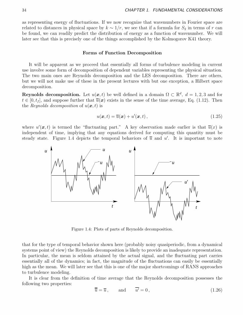
34 CHAPTER 1. FUNDAMENTAL CONSIDERATIONS
as representing energy of fluctuations. If we now recognize that wavenumbers in Fourier space arerelated to distances in physical space by k ∼ 1/r, we see that if a formula for S2 in terms of r canbe found, we can readily predict the distribution of energy as a function of wavenumber. We willlater see that this is precisely one of the things accomplished by the Kolmogorov K41 theory.
Forms of Function Decomposition
It will be apparent as we proceed that essentially all forms of turbulence modeling in currentuse involve some form of decomposition of dependent variables representing the physical situation.The two main ones are Reynolds decomposition and the LES decomposition. There are others,but we will not make use of these in the present lectures with but one exception, a Hilbert spacedecomposition.
Reynolds decomposition. Let u(x, t) be well defined in a domain Ω ⊂ Rd, d = 1, 2, 3 and fort ∈ [0, tf ], and suppose further that u(x) exists in the sense of the time average, Eq. (1.12). Thenthe Reynolds decomposition of u(x, t) is
u(x, t) = u(x) + u′(x, t) , (1.25)
where u′(x, t) is termed the “fluctuating part.” A key observation made earlier is that u(x) isindependent of time, implying that any equations derived for computing this quantity must besteady state. Figure 1.4 depicts the temporal behaviors of u and u′. It is important to note
t t
u u
u
u
u′
u
Figure 1.4: Plots of parts of Reynolds decomposition.
that for the type of temporal behavior shown here (probably noisy quasiperiodic, from a dynamicalsystems point of view) the Reynolds decomposition is likely to provide an inadequate representation.In particular, the mean is seldom attained by the actual signal, and the fluctuating part carriesessentially all of the dynamics; in fact, the magnitude of the fluctuations can easily be essentiallyhigh as the mean. We will later see that this is one of the major shortcomings of RANS approachesto turbulence modeling.
It is clear from the definition of time average that the Reynolds decomposition possesses thefollowing two properties:
u = u , and u′ = 0 , (1.26)
1.4. DEFINITIONS, MATHEMATICAL TOOLS, BASIC CONCEPTS 35
with the first of these being obvious, and the second following from the first. These will be crucialin our later derivation of the RANS equations, and the reader is encouraged to show that theseequalities hold.
LES decomposition. The LES decomposition was introduced by Deardorff [10] and was firstanalyzed in detail for the incompressible N.–S. equations by Leonard [76]. It is constructed byapplying a local spatial filter (or in the simplest case, spatial average) to all appropriate variables.It is interesting to note that the averaging originally proposed by Reynolds [16] was spatial ratherthan temporal; hence, it can be seen that Deardorff’s approach was rather close to Reynolds’ originalformulation. Despite this, current applications of Reynolds averaging employ time averaging, andLES uses a spatial filter, as we will now describe.
We will see below that the LES decomposition can be interpreted as a Hilbert space decompo-sition, so we begin by assuming u(x, t) ∈ L2(Ω) × C1(0, tf). Then we write the LES decompositionas
u(x, t) = u(x, t) + u′(x, t) . (1.27)
In this decomposition u is usually termed the large- or resolved-scale part of the solution, and u′
is called the small-scale, or subgrid-scale, or unresolved part. It is important to note that bothresolved and unresolved scales depend on both space and time, and this is a major distinctionand advantage compared with the Reynolds decomposition. In Eq. (1.27) u is formally the filteredsolution corresponding to Eq. (1.15). From this it is easily shown that, in general,
˜u 6= u , and u′ 6= 0 , (1.28)
(although there are special cases for which equalities do hold). The reader may wish to investigatethis.
This lack of equality in Eqs. (1.28) significantly complicates derivation of the usual LES formu-lations in comparison with RANS approaches and, in particular, leads to Leonard and cross stressesin addition to the usual Reynolds stress as will be seen in Chap. 3. On the other hand, once theformulation has been developed there is little additional complication, and the LES equations arequite similar to the RANS equations with one major exception: the RANS equations are formallyindependent of time, while the LES equations are valid for time-dependent calculations.
Hilbert space decomposition. The final decomposition we consider here is a mathematical onethat is closely related to the LES decomposition. It is the ability to construct such decompositionsthat is crucial to obtaining numerical approximations to solutions of the N.–S. equations. In par-ticular, because of the properties of the Hilbert space L2 we can express the Fourier representation,Eq. (1.6), as
f(x) =
N∑
|k|≥0
akϕk(x) +
∞∑
|k|=N+1
akϕk(x) . (1.29)
Each series on the right-hand side is an element of a subspace of L2, and due to orthogonality ofthe ϕks these subspaces do not intersect. Furthermore, as N → ∞, the first term on the right-handside, alone, more closely approximates f , and we view the second term as the remainder of theseries representation.
If we draw an analogy between the terms of the LES decomposition (1.27) with those in theabove expression, we expect that the large-scale part of LES will converge to a solution of the N.–S.equations as the discrete resolution of the solution procedure is increased provided the SGS modelis constructed so that the small-scale part (corresponding to the series remainder) approaches zeroin this same limit. We will later see that, indeed, this is the case, thus providing assurance thatLES is mathematically well founded. We remark that no such convergence result can be deduced
36 CHAPTER 1. FUNDAMENTAL CONSIDERATIONS
for RANS methods. In particular, it should be clear from Fig. 1.4 that u′ cannot be viewed asthe remainder of a Fourier series expansion and moreover, in light of its physical interpretation, itcannot be considered to be small, in general.
Cartesian Tensor Notation
Cartesian tensor notation provides a short-hand that is widely used in fluid dynamics, especiallyin the context of classical turbulence analyses. We will provide a brief treatment of this in thecurrent section since it will be necessary to occasionally use it later.
We begin by noting that the mathematical description of a tensor (over a vector space) is amulti-linear form (see, e.g., Bishop and Goldberg [97]), meaning that a tensor is a multi-variableconstruct that satisfies the definition of linearity in each of its variables, separately. Within thisframework we might represent a tensor as F (V1, V2, . . . , VN) with F being linear with respect toeach of the N vector spaces, Vi , i = 1, . . . , N , appearing in its argument. But Cartesian tensors aremuch less general (as the name suggests), and unlike the preceding expression which is coordinatefree, Cartesian tensors are presented in terms of Cartesian coordinates, the specific orientationand origin of which must be specified (in terms of a basis set) to completely define such a tensor.Indeed, from a purely mathematical perspective, what are often called tensors are actually a specificrepresentation of a tensor in terms of coordinates. We note that in our present context, scalars aretensors of rank zero; vectors have rank one, and matrices have rank two. The term “tensor” willthus imply rank two, i.e., a matrix, unless noted otherwise.
Cartesian tensor notation is concise because of its use of indexing and operations specificallyassociated with this indexing. For example, the velocity vector is represented as
U = (u1, u2, u3)T
(= (u, v, w)T
),
and spatial coordinates as x = (x1, x2, x3)T . Operations with Cartesian tensors involve implied
summation over repeated indices (Einstein summation); so, for example, the divergence of thevelocity field can be expressed as
∇ · U =∂ui
∂xi
≡3∑
i=1
∂ui
∂xi
=∂u1
∂x1
+∂u2
∂x2
+∂u3
∂x3
(=
∂u
∂x+
∂v
∂y+
∂w
∂z
).
We observe that the index i appears in both numerator and denominator of the tensor representation∂ui/∂xi, and so is “repeated.” But this is not the only form of repeated indices. For example, if S
denotes the strain rate tensor with elements
Sij ≡1
2
(∂ui
∂xj+
∂uj
∂xi
),
then SikSkj denotes the matrix multiplication
S S =
3∑
k=1
SikSkj ∀ i, j = 1, 2, 3.
Using these constructs permits expressing the incompressible N.–S. equations given in Eqs. (1.1)as
∂ui
∂xi= 0 , (1.30a)
∂ui
∂t+ uj
∂ui
∂xj= −
∂P
∂xi+ ν
∂2ui
∂xj∂xj, i = 1, 2, 3 . (1.30b)
1.4. DEFINITIONS, MATHEMATICAL TOOLS, BASIC CONCEPTS 37
Although this notation seems not to provide any significant advantages in expressing the N.–S.equations, themselves (and, in fact, it doesn’t), it is very effective in concisely representing theRANS equations and various quantities associated with turbulence models constructed for use withthese equations. This will be apparent in the sequel.
We end this description of Cartesian tensors by introducing two specific items that are widelyused to further collapse notation. The first is the Kronecker δ which, in the present context, is usedto represent the identity matrix:
δij ≡
1 if i = j , i, j = 1, 2, 3 ,0 otherwise .
(1.31)
The second is what is called the permutation tensor, defined as
ǫijk ≡
1 for any permutation of i, j, k = 1, 2, 3 ,−1 for non-repeating combinations of i, j, k that are not permutations ,
0 if any two indices are repeated .(1.32)
We leave as an exercise to the reader demonstration that the curl of the velocity field can be veryconcisely expressed in terms of the permutation tensor as
(∇×U)i = ǫijk∂uk
∂xj.
Finally, following Wilcox [98], we note that there is an identity relating δij and ǫijk:
ǫijkǫist = δjsδkt − δjtδks . (1.33)
Proof of this is left as an exercise.
1.4.3 Further basic concepts
In this section we consider some further, fairly general, basic ideas associated either indirectly, ordirectly, with turbulence. In the first of two subsections we treat some basic properties of theN.–S. equations since, as we will emphasize throughout these lectures, these equations are nowalmost universally accepted as providing the correct description of turbulent flows. Much of whatis presented in this subsection is extracted from Frisch [80] or from Foias et al. [89].
In a second subsection we present a number of somewhat more physically-oriented concepts that,while they are not necessarily related to any particular turbulence model, have played significantroles in setting the “way of seeing” turbulence that has contributed to the form of a number ofmodels. This information comes from a variety of sources, but mainly from [80] and [7].
Mathematical Properties of the N.–S. Equations
In this section we consider some mathematical aspects of the N.–S. equations that have hadmajor impacts on recent ideas concerning turbulence, and also some concepts that have influencedthe nature of models as well. We begin with a discussion of symmetries of the N.–S. equations asdescribed in [80], the most important of which is Galilean invariance. We follow this with a briefdiscussion of current knowledge on existence, uniqueness and regularity of N.–S. solutions, and weconclude the section by constructing the Galerkin approximation to the N.–S. equations.
Symmetries, symmetry groups. Frisch [80] notes that symmetry is a term employed by theoret-ical physicists when referring to invariance groups of a dynamical theory. (For each symmetry there
38 CHAPTER 1. FUNDAMENTAL CONSIDERATIONS
is an associated “conservation law.”) We observe that group has a precise, and somewhat abstract,mathematical meaning that we do not need to explore for the present lectures. In any case, supposeG is such a group, and suppose U is a solution to the (incompressible) N.–S. equations. If g ∈ G
and gU is also a solution to the N.–S. equations, then G is a symmetry group for these equations.We remark that the “similarity transformations” arising in boundary-layer theory provide a familiarexample of such groups.
A total of six symmetries of the N.–S. equations are discussed in [80]; but, as noted there, somedo not hold for high Re, and others do not hold for low Re. There are three that are valid symmetrygroups independent of Re (but with other restrictions) and that are of particular importance. Theseare the following:
i) space translations gspaceρ : t, r, U 7−→ t, r + ρ, U , ρ ∈ Rd d = 1, 2, 3;
ii) time translations gtimeτ : t, r, U 7−→ t + τ, r, U , τ ∈ R ;
iii) Galilean transformations gGalV : t, r, U 7−→ t, r + V t, U + V , V ∈ Rd.
In these mappings ρ, τ and V represent any bounded constant with the specified dimension. Thus,proof that space and time translations are symmetry groups of the N.–S. equations is direct, andwe leave this as an exercise for the reader.
Galilean invariance, described briefly in Def. 1.73, is one of the most important properties ofthe N.–S. equations because, as observed earlier, without it we would find it impossible to com-pare fluid experiments performed in different parts of the world. Indeed, if the N.–S. equationswere not Galilean invariant, this would be a sure sign that they could not properly describe fluidmotion. It turns out that this universal symmetry is often violated by RANS turbulence models(see, e.g., Speziale [99]), and much effort has gone into modifying such models to avoid this phys-ical discrepancy—at the expense of relative simplicity. Frisch notes that the key to proving thissymmetry is to show cancellation of terms arising from U t and U · ∇U under the transformation.We will demonstrate this here for the 1-D Burgers’ equation and leave the proof for the completeN.–S. system as an exercise.
To begin, recall that Burgers’ equation is a 1-D model equation possessing all of the same typesof terms as do the momentum equations of the N.–S. system. Thus, it can be expressed as
ut + uux = νuxx , (1.34)
where ν can be viewed as a viscosity, or the reciprocal of the Reynolds number. Now for a generaltransformation, say T , we have
T :
(xt
)−→
(ξ(x, t)τ(x, t)
)with T−1 :
(ξτ
)−→
(x(ξ, τ)t(ξ, τ)
).
Equation (1.34) is invariant under the transformation T if we can show that
uτ + uuξ = νuξξ . (1.35)
That is, the form of the equation remains the same after transformation. We leave it to the readerto demonstrate that this does not happen, in general, that is, for arbitrary general transformations.
In the specific case of the Galilean transformation we have
gGalv : ξ = x + vt , τ = t ,
and (gGal
v
)−1: x = ξ − vτ , t = τ .
1.4. DEFINITIONS, MATHEMATICAL TOOLS, BASIC CONCEPTS 39
But since the dependent variable is also transformed in this case, for invariance to hold we musthave
wτ + wwξ = νwξξ ,
with w = u + v. Thus, we must show that
(u + v)τ + (u + v)(u + v)ξ = ν(u + v)ξξ (1.36)
is the same as Eq. (1.34).We first observe that since v is a constant, the above collapses to
uτ + (u + v)uξ = νuξξ . (1.37)
Next, from properties of transformations rather generally, and the inverse function theorem inparticular, we know that
u(ξ, τ) = u(ξ(x, t), τ(x, t)) = u(x(ξ, τ), t(ξ, τ)) ,
under reasonable smoothness assumptions, which clearly hold for the Galilean transformation, itself,although possibly not for dependent variables of the differential equation(s). Hence, we have
∂u
∂τ=
∂u
∂x
∂x
∂τ+
∂u
∂t
∂t
∂τ= −v
∂u
∂x+
∂u
∂t,
and similarly,∂u
∂ξ=
∂u
∂x
∂x
∂ξ+
∂u
∂t
∂t
∂ξ=
∂u
∂x.
From this it follows that uξξ = uxx. Then Eq. (1.37) becomes
−v∂u
∂x+
∂u
∂t+ (u + v)
∂u
∂x= ν
∂2u
∂x2,
and we see that the cancellation mentioned earlier indeed occurs, completing proof of Galileaninvariance of Burgers’ equation. A quite similar proof can be applied for the N.–S. equations.
As is noted in [80], Chap. 1, with the exception of Galilean invariance the above symmetriesare broken as Re is increased. But once Re is sufficiently high to admit fully-developed turbulentbehavior, the symmetries are restored in a statistical sense provided there is no directional forcing.However, we remark that such forcing is nearly always present in actual flows, so it is only in thecase of high-Re homogeneous turbulence that symmetries, even in the statistical sense, are trulyrestored.
Existence, uniqueness, regularity of N.–S. solutions. Here we briefly describe current knowl-edge of the nature of solutions to the Navier–Stokes equations. This is particularly important be-cause these equations must be solved by numerical methods implemented on digital computers,and the nature of solutions directly influences what types of methods will be effective, and whattypes will not. We encourage the reader to consult Foias et al. [89] for a more thorough treatmentcorresponding to the present discussions. We begin by stating the main results in an informal way,without defining terms. We then proceed to, again rather informally, define terms and explainconsequences of the results.
Results for the N.–S. equations can be classified as pertaining to 2-D or to 3-D flows, and as towhether they relate to weak or strong solutions. With regard to these classifications, it is usuallysaid that essentially everything worth proving for 2-D problems has been proven. In particular,existence and uniqueness of solutions, both weak and strong, have been proven for all time beyond
40 CHAPTER 1. FUNDAMENTAL CONSIDERATIONS
any specified initial time for quite reasonable (physically) problems. In 3D, long-time existencecan be demonstrated for weak solutions, but uniqueness has not been proven for this case. On theother hand, only short-time existence has been proven for 3-D strong solutions, but it is knownthat these are unique. Especially with regard to existence of strong solutions, the constraints thatmust be imposed on the shape of the domain Ω (in particular, smoothness of ∂Ω), the boundaryand initial conditions, and especially on body-force terms and Reynolds number (∼viscosity) canbe quite stringent if solutions are to be proven to exist for any but very short times.
We recall that a weak solution is one that is not sufficiently differentiable to be substitutedinto the differential form of the equations, and instead only satisfies an integral (weak) form ofthe equations. The Galerkin approximation to be presented next is one such form. A strongsolution is one that is sufficiently smooth to satisfy the original differential equation(s) in the senseof L2. It is important to note, however, that this is not the same as a classical solution which issufficiently differentiable to permit substitution into the differential equation at all points of theproblem domain. In the case of a strong solution there can exist a nonempty set of points withinthe domain at which this cannot be done.
In summary, in 2D it can be proven that both weak and strong solutions to the N.–S. equationsexist for all time and are unique; hence, they are equivalent. In 3D, weak solutions exist for alltime, but may not be unique; and strong solutions are unique, but existence can be proven for onlyfinite times.
There are several important consequences of these results. First, since it is widely accepted thatturbulence is, indeed, three dimensional, inability to prove long-time existence of strong solutionsto the 3-D N.–S. equations might cast some doubt on acceptance of these equations as the correctrepresentation of turbulent flow. In particular, without long-time existence it is difficult to arguethat stationary solutions even exist, and analysis of these is just as important in modern theoriesas in classical ones. But it is usually felt that lack of the desired long-time existence proof reflectsmore on inadequacy of current mathematical techniques than suggests an inappropriateness of theN.–S. equations. In support of this is the general success of DNS, not only in the sense of beingable to quite accurately reproduce known turbulence results but also in terms of making predictionslater confirmed in laboratory experiments—although only for relatively low Re. (DNS has yet to beperformed for high-Re flows for reasons we have mentioned previously and which we will considerin detail below.)
But even if it should happen that one day it is proven that long-time strong solutions do notexist, this removes only uniqueness and regularity; we already know 3-D weak solutions exist for alltime. They simply are not very smooth, and they might not be unique.
Second, even in the context of strong solutions, which satisfy the N.–S. equations only in thesense of L2, i.e., ∫
Ω
(U t + U · ∇U + ∇P − ν∆U )2 dx → 0
as the number of modes in a Fourier representation (or, equivalently, the number of grid points ina finite-difference, or finite-volume, or finite-element approximation) → ∞, is the fact that higherderivatives beyond second that appear in representations of the truncation error of typical discretemethods may not exist, and thus cannot be bounded. This implies that attempting to employ high-order methods for discretization of the N.–S. equations in strong form is likely doomed to fail, at leastat high Re, unless fairly elaborate filtering is also used. On the other hand, spectral methods will notsuffer from this difficulty and are of “infinite-order” accuracy for smooth solutions. Furthermore,finite-element methods (FEMs) are oftened formulated for a weak form of the equations beingsolved, so higher-order FEMs should work satisfactorily if properly formulated.
Finally, we observe that if it turns out that only weak solutions exist for long times, and inaddition they cannot be proven to be unique, it will then become very important for experimentalists

1.4. DEFINITIONS, MATHEMATICAL TOOLS, BASIC CONCEPTS 41
to attempt to find multiple solutions arising from the same set of conditions (and there will be manysignificant difficulties with such attempts). We note that this situation is distinct from sensitivityto initial conditions which has always been observed in laboratory experiments, but, on the otherhand, could still be influenced by this phenomenon. Instead, it corresponds to a situation forwhich, in the dynamical systems sense, there exists at least two attractors for the “same” basin ofattraction. This can occur for a basin of attraction whose topology is so fractally intertwined thatextremely small changes in initial data lead to long-time behavior associated with entirely differentattractors—as opposed to simply different trajectories on the same attractor as occurs in the usualsense of SIC. Clearly, there are stability issues to be addressed here—probably via mathematicsinstead of laboratory experiments—and this might offer an approach to proving uniqueness of weaksolutions; in particular, possibly there is only a single stable one. At the same time, there seem tobe a number of published results (usually not very well supported) suggesting such a nonuniquenessproperty. Both experimental and computational studies have occasionally indicated this.
Galerkin approximation to the N.–S. solutions. For simplicity we treat the 2-D dimensionlessform of Eqs. (1.1) in the absence of body forces. We express these here as
ux + vy = 0 . (1.38a)
ut + (u2)x + (uv)y = −px +1
Re∆u , (1.38b)
vt + (uv)x + (v2)y = −py +1
Re∆v , (1.38c)
and we represent the dependent variables in Fourier series:
u(x, y, t) =∞∑
k
ak(t)ϕk(x, y) , (1.39a)
v(x, y, t) =
∞∑
k
bk(t)ϕk(x, y) , (1.39b)
p(x, y, t) =
∞∑
k
ck(t)ϕk(x, y) , (1.39c)
with k ≡ (k1, k2)T . The lower bound for components of this wavevector is typically one of −∞, 0
or 1. Also, an analogous expansion would be needed for dependent variables contained in a bodyforce if one were present.
For convenience we will assume the domain Ω is a rectangle and that the boundary conditionsused with Eqs. (1.38) are periodic. Although this is a quite restrictive situation, our main goalhere is to introduce some mathematical notions associated with the N.–S. equations when viewed inFourier space, so the overall simplicity of this arrangement is an advantage. It is important to note,however, that it is difficult to lift these conditions and retain a numerically efficient procedure; asa consequence, most computer implementations of this method are quite similar to the version wewill discuss here.
In light of the periodicity conditions it is natural to employ complex exponentials as basisfunctions; that is, we set
ϕk(x, y) = eik·x = ei(k1x+k2y) = eik1xeik2y . (1.40)
The last form on the right is often termed a “tensor product” basis because its two factors aredefined in an uncoupled way on subsets of two separate copies of R1. (Clearly, an analogous formexists for 3D.)
42 CHAPTER 1. FUNDAMENTAL CONSIDERATIONS
To begin construction of the Galerkin form of Eqs. (1.38) we start with the simplest, Eq. (1.38a),the divergence-free condition, or continuity equation. We substitute Eqs. (1.39a) and (1.39b) intothis equation and commute summation and differentiation to obtain
i∞∑
k
(k1ak + k2bk)ϕk = 0 .
Since this must hold at (almost) all points of Ω, and ϕk 6≡ 0, we must have
k1ak + k2bk = 0 ∀ k . (1.41)
Similarly, if we substitute the expansions (1.39) into the x-momentum equation (1.38b), weobtain
∂
∂t
∑
ℓ
aℓϕℓ +∂
∂x
∑
ℓ,m
aℓamϕℓϕm +∂
∂y
∑
ℓ,m
aℓbmϕℓϕm =
−∂
∂x
∑
ℓ
cℓϕℓ +1
Re
[∂2
∂x2
∑
ℓ
aℓϕℓ +∂2
∂y2
∑
ℓ
aℓϕℓ
].
Again commuting summation and differentiation yields∑
ℓ
aℓϕℓ + i∑
ℓ,m
(ℓ1 + m1)aℓamϕℓϕm + i∑
ℓ,m
(ℓ2 + m2)aℓbmϕℓϕm =
− i∑
ℓ
ℓ1cℓϕℓ −1
Re
∑
ℓ
(ℓ21 + ℓ2
2
)aℓϕℓ .
It can be seen that the solutions (the aℓs, bℓs, cℓs) to this equation can be complex, but we areonly interested in those that are real if we are considering solutions corresponding to actual physicsof fluid flow. Indeed, if we had used sine and cosine as basis functions rather than the otherwisemore convenient complex exponentials, this would not have been a concern. Furthermore, the readerwill recall that sines and cosines may be expressed in terms of complex exponentials in any case.This suggests that a means of avoiding the potentially complex solutions should be available. Infact, all that is required is setting a−k = ak, where the overbar here denotes complex conjugate,and the imaginary parts become zero (see, e.g., [89]).
This permits us to consider the preceding equation without the imaginary factors i and proceedformally. (This description is lacking some details, but it is sufficient for our purposes.) We nowuse orthonormality of ϕk and form inner products of each of these with the above equation toobtain
ak +∑
ℓ,m
A(1)kℓmaℓam +
∑
ℓ,m
B(1)kℓmaℓbm = −k1ck −
|k|2
Reak , ∀ −∞ < k < ∞ . (1.42)
In these equations the A(1)kℓms and B
(1)kℓms, sometimes termed Galerkin triple products, are defined
as, for example,
A(1)kℓm ≡ (ℓ1 + m1)
∫
Ω
ϕkϕℓϕm dx , (1.43)
where the (1) superscript denotes the x-momentum equation. Clearly, an analogous result holds forthe y-momentum equation:
bk +∑
ℓ,m
A(2)kℓmbℓam +
∑
ℓ,m
B(2)kℓmbℓbm = −k2ck −
|k|2
Rebk . (1.44)

1.4. DEFINITIONS, MATHEMATICAL TOOLS, BASIC CONCEPTS 43
We remark that this is the step (constructing the inner products) that casts the N.–S. equationsin a weak, integral form, but we should also note that the Fourier representations only guaranteeconvergence in L2 in any case; so we would not necessarily expect strong solutions, in general.
At this point we should recall that it is generally possible to eliminate pressure from the mo-mentum equations. If we view Eqs. (1.42) and (1.44) as a vector equation for the vector (ak, bk) ofFourier coefficients, we can take the dot product of this with k = (k1, k2)
T to obtain
k1ak + k2bk +∑
ℓ,m
[k1
(A
(1)kℓmaℓam + B
(1)kℓmaℓbm
)+ k2
(A
(2)kℓmbℓam + B
(2)kℓmbℓbm
)]
= −(k2
1 + k22
)ck −
|k|2
Re(k1ak + k2bk) ∀ −∞ < k < ∞ .
We observe that this merely corresponds to constructing the divergence of the N.–S. equations inFourier space.
From Eq. (1.41) we see that the first term on the left-hand side and the second on the right-handside are both identically zero, and moreover, we can solve what remains for ck in terms of only theaks and bks:
ck = −1
|k|2
∑
ℓ,m
[k1
(A
(1)kℓmaℓam + B
(1)kℓmaℓbm
)+ k2
(A
(2)kℓmbℓam + B
(2)kℓmbℓbm
)]. (1.45)
This implies, as we expected, that Eqs. (1.42) and (1.44) can be expressed in a form that is indepen-dent of the pressure. Beyond this it explicitly demonstrates the quantitative dependence of pressureon the velocity field—in Fourier space. It is interesting to note the tendency to view pressure asthe driving force that sets velocity components of the N.–S. equations, and this is to some extenttrue for externally-applied (boundary) pressures. But we see from Eq. (1.45) that internal staticpressures are set by the velocity field within the confines of the divergence-free condition—just theopposite of the usual (physical) interpretation.
It is worthwhile to examine some of the details of the Galerkin form of the N.–S. equations.We first make the obvious observation that this form comprises a system of equations for the timeevolution of the Fourier coefficients of the velocity components, and as such is a dynamical systemrecall (Def. 1.18). Furthermore, at each instant in time for which ak(t) and bk(t) are known, theFourier coefficients for pressure can be calculated directly from Eq. (1.45); and these coefficientscan be inserted into Eqs. (1.39) to obtain values of u, v and p at any point x ∈ Ω. Of course,in practice these Fourier representations can contain only a finite number N of terms, so theresults are only approximate. But at least for solutions possessing a high degree of regularity,Fourier series converge very rapidly (in fact, exponentially), so not many terms are needed toobtain accurate approximations. For the reader interested in this feature, as well as numerous otherdetails associated with these types of approximations, the monograph by Canuto et al. [100] isrecommended.
Our main purpose in presenting the Galerkin form of the N.–S. equations is to demonstrate howthis Fourier-space representation can be used to deduce qualitative mathematical (and physical)features of N.–S. flows. We consider only the x-momentum equation (1.42); but the same treat-ment applies to y-momentum, and extension to 3-D flows occurs in a natural way. We begin bytemporarily neglecting all nonlinear terms in Eq. (1.42), with ck also eliminated in light of (1.45).Then what remains is
ak = −|k|2
Reak , (1.46)
the solution of which is
ak(t) = ak(0)e−|k|2
Ret , (1.47)

44 CHAPTER 1. FUNDAMENTAL CONSIDERATIONS
where
ak(0) ≡
∫
Ω
u0(x)e−ik·x dx , (1.48)
with u0(x) denoting the x component of initial velocity.Clearly, this solution decays in time and approaches zero as t → ∞. Moreover, the rate at
which this occurs is |k|2/Re. In particular, for fixed Re higher wavenumber Fourier modes decayfaster than do lower ones. From a mathematical perspective this suggests (but does not prove)convergence of the Fourier series representation and, hence, existence of solutions of the form Eqs.(1.39). On the other hand, if |k| is fixed, then the rate of decay of ak decreases with increasing Re.Now if we recall that the right-hand side of Eq. (1.46) is precisely the Fourier-space representationof the viscous terms of Eq. (1.38b), we see that we can associate the rate of decay of ak withphysical viscous dissipation; in particular, increasing Re implies decreasing viscous dissipation, andconversely. While we will later obtain a specific formula for viscous dissipation rate, per se, inphysical space (which is not the same as the viscous terms of the N.–S. equations), it is clear thatthese terms—and only these terms—contribute to decay of solutions directly.
We now consider effects of the nonlinear terms. To do this we first drop the linear viscousdissipation term from Eq. (1.42), and we also drop the term containing ck arising from the pressuregradient in Eq. (1.38b) since, as can be seen from Eq. (1.45), this is directly related to the nonlinearterms; so nothing is lost at the qualitative level by ignoring it. Then we are left with
ak = −∑
ℓ,m
[A
(1)kℓmaℓam + B
(1)kℓmaℓbm
]. (1.49)
We first observe that when ℓ = m a quadratic term appears in the equation. It is worthwhile toconsider the effects of this alone since an analytical solution can be obtained, and this will provideat least some insight into the qualitative behavior of the nonlinear terms in general. Thus, we solvethe initial-value problem
ak = −A(1)a2k , (1.50)
with ak(0) again given by Eq. (1.48) and subscript notation for A(1)kℓm suppressed. We leave as a
simple exercise to the reader demonstration that
ak(t) =1
A(1)t + 1/ak(0).
It is clear from this that if A(1)ak(0) > 0, then |ak| → 0 as t → ∞, although only algebraically. Butif A(1) and ak(0) are of opposite signs, ak(t) → ∞ can occur in finite time. This implies a potentialfor very ill behavior (including nonexistence after only a finite time) of N.–S. solutions. In 2D itis known that this does not actually occur (which implies this simplification is not an extremelyaccurate model); but as we have already indicated, this possibility has not been eliminated in 3D—itis possible that 3-D solutions to the N.–S. equations fail to exist after a finite time.
There is a further aspect of the behavior of the terms on the right-hand side of Eq. (1.49) thatdeserves mention. It is that such nonlinearities can generate new Fourier modes not present in theoriginal representation (or in initial data for the problem). Here we consider only the first advectiveterm of the x-momentum equation, (u2)x, and recall its Fourier representation:
(u2)x =∂
∂x
N∑
ℓ,m
aℓamϕℓϕm ,
written now for only a finite number N of Fourier modes, as would be required for computerimplementation.
1.4. DEFINITIONS, MATHEMATICAL TOOLS, BASIC CONCEPTS 45
Now if the basis set ϕk is similar to complex exponentials or trigonometric functions we seethat, e.g.,
ϕℓ(x)ϕm(x) = eiℓ·xeim·x = ei(ℓ+m)·x .
Since each of ℓ and m can be as large as N , their sum is often greater than N , and the correspondingnonlinear term aℓam generates solution behaviors that cannot be resolved by the given representa-tion. We note here that this does not occur for the Galerkin procedure due to the values taken onby the Galerkin triple products, and due to the general global nature of the Fourier coefficients; butit does occur for the various Fourier collocation methods that are widely used as a more efficientalternative to the Galerkin procedure (see [100]) in the context of both DNS and LES. Moreover,it is easily argued that this must occur for finite-difference and finite-volume methods as well.
Finally, we emphasize that the actual time evolution of each of the aks is effected by combinationsof all the abovementioned behaviors, and as a consequence solutions can be very complicated—andvery difficult to simulate. In particular, it should be clear that the kth Fourier coefficient, ak, can beaffected by coefficients corresponding to wavenumbers both less than and greater than k through thenonlinear terms of the Galerkin representation (including those arising from the pressure gradient).But the specific outcomes of such interactions are strongly influenced by the dissipation induced bythe linear (viscous) terms. We recall that the degree of this is set by the combination of Reynoldsnumber and the specific wavenumber under consideration.
General (mostly) Physical Concepts from Turbulence
In this section we begin by presenting some mostly heuristic ideas concerning the nature andcauses of turbulence, relating these to the mathematical constructs of the preceding section. We thendescribe the various well-known length and time scales that occur in turbulent flows, again showinghow these are associated with the mathematics—in particular, where they reside in the energyspectrum. In connection with the relationship between length and time scales we will introduce theoften-used (especially in analysis of experimental data) Taylor hypothesis. Then we provide moredetails on homogeneous and isotropic turbulence, and we conclude the discussions with some basicanalysis of the law of the wall.
What is turbulence?—and where does it come from? In some respects, it is not clear that theanswer to either of these questions is completely known. Certainly, from a physical standpoint thereare many unresolved issues. Earlier in this chapter we gave an extensive list of characterizations ofturbulence and noted that turbulent flows always exhibit some (and maybe all) of these features;but this does not really define physical turbulence. On the other hand, we were able to at leastpropose a mathematical definition, namely, 3-D, chaotic solutions to the Navier–Stokes equationsat high Reynolds number. But this “definition” is certainly not universally accepted for reasons wewill discuss later in these lectures. So, the answer to the first question seems to yet be lacking, atleast on purely physical grounds. We remark, that part of the difficulty seems to be that there areso many possible characterizations that do not all occur in every flow situation intuitively viewedas turbulent that evidently turbulence may be more than a single phenomenon. If so, this wouldsuggest that the mathematical definition might be the best we can obtain.
Before addressing the second question we here introduce a list of misconceptions associated withturbulence. These have been extracted from a somewhat longer list provided by Tsinober [3] inAppendix D of his book.
‘Statistical’ and ‘structural’ contrapose each other.
Turbulence possesses a random (quasi)-Gaussian background.
Kolmogorov picture is structureless and quasi-Gaussian.
46 CHAPTER 1. FUNDAMENTAL CONSIDERATIONS
Large scales and small scales are decoupled.
‘Eddy viscosity’ and ‘eddy diffusivity’ explain the enhanced transfer rates of momentum, energyand passive objects.
Spatial fluxes represent ‘cascade’ in physical space.
Vorticity amplification is a result of the kinematics of turbulence.
Strain rate in turbulent flows is irrotational.
Enhanced dissipation in turbulent flows is due to vortex stretching.
Each of these has been touted as an important characterization of turbulence by numerous au-thors, but in [3] they are all shown to imply serious logical (and physical—based on experimentalobservations) flaws.
The second question can be answered somewhat more satisfactorily from a physical standpoint;and, fortunately, the answer is in accord with the mathematics of the N.–S. equations. In particular,it is well understood that turbulence only occurs in flows exhibiting fairly large velocity gradients.The simplest familiar example is pipe flow, but the descriptions we will provide work equally wellfor essentially any flow; only the mechanism for producing the velocity gradients would change.
We first observe that pipe flow is laminar until a Reynolds number of approximately 2000 isreached, whereupon transition begins. Recall that, in a pipe, the velocity satisfies the no-slipcondition at the walls and adjusts to the centerline velocity across the radius of the pipe. Hence,there is a velocity gradient that is largest at the pipe wall. Furthermore, it is easy to imaginethat if the wall of the pipe is rough the velocity gradients might be locally (but not necessarilyuniformly) higher than in the smooth-wall case; and, indeed, for pipes having extremely smoothwalls, it is possible to delay transition to turbulence until the Reynolds number is well above 50,000.Furthermore, there are no known uniform flows—either physically or mathematically—that exhibittransition.
From a purely mathematical standpoint, it is well known (and not difficult to show) that Fourierseries converge far more slowly for functions having large derivatives than for very smooth, well-behaved functions. This, in turn, implies that larger wavenumbers will still provide significantcontributions, and in the context of the Galerkin approximation to the N.–S. equations given above,this means that even higher wavenumber information will be generated spontaneously. Then, if Re islarge, such wavenumber data will not be readily damped by the viscous terms, and chaos generatedin the nonlinear terms will dominate the behavior—hence, turbulence. Conversely, if a flow hasonly small gradients, the linear viscous terms of the Fourier representation very effectively dampthe solutions, thus maintaining, or even further reducing, the small gradients.
It is important to also mention here the classical view of this interpretation as given, for example,in Tennekes and Lumley [7]. In that reference, as well as many others, the role of vorticity is stressed,in conjunction with the energy cascade described earlier in Def. 1.68. In particular, it is arguedthat energy is usually supplied to a turbulent flow through mechanisms that create large vortices.It is hypothesized (a la Richardson [4]) that these vortices, usually referred to as “eddies,” aresomehow broken into smaller ones, that themselves split into still smaller ones, and so on, untilthey are sufficiently small as to be dissipated by viscosity. We remark, however, that vorticity,the quantification of the strength of such vortices, is not actually physics—vorticity is a purelymathematical definition. Indeed, vorticity is constructed from the velocity gradients describedabove—which are physics: the amount velocity changes over a given distance. So, it is not clearthat a viewpoint expressed in terms of vorticity and eddies contributes to physical understandingeven if it happens to be correct. But in addition, careful examination of most physical flows
1.4. DEFINITIONS, MATHEMATICAL TOOLS, BASIC CONCEPTS 47
does not clearly show sequences of sizes of vortices simply breaking or splitting as suggested bythis simplistic scenario. Moreover, this view is not completely consistent with mathematics ofthe Galerkin approximation to the N.–S. equations. We noted in earlier discussions that Fouriercoefficients (think “energy”—i.e., the L2 norm) are influenced by behaviors at both higher and lowerwavenumbers; hence, energy might be transferred in either direction, at least locally, in wavenumberspace. But this is not included (permitted?) in the energy cascade description involving breakupof eddies.
Length and time scales of turbulence. One of the items in our earlier list of characterizationsof a turbulent flow at the end of Sec. 1.2 was its wide range of length and time scales. In fact, ifsuch scales did not cover wide ranges, the “turbulence problem” would have been solved long ago.In such a case, the N.–S. equations could be easily and efficiently solved on a digital computer foressentially any physical flow. But as will be evident as we proceed, it is precisely this feature ofturbulent flow that precludes use of DNS in most flow situations. Thus, it is especially importantto understand some of the details.
We begin by noting that there are, in general, four main sets of scales in a turbulent flow (theremay be more if other physical phenomena, e.g., heat transfer and/or combustion are important);these are:
i) the large scale, based on the problem domain geometry,
ii) the integral scale, which is an O(1) fraction (often taken to be ∼ 0.2) of the large scale (andtermed the “outer scale,” especially in Russian literature),
iii) the Taylor microscale which is an intermediate scale, basically corresponding to (actually,within) Kolmogorov’s inertial subrange, and
iv) the Kolmogorov (or “dissipation”) scale which is the smallest of turbulence scales (called the“inner scale” in Russian works).
Before considering details, it is worthwhile to first qualitatively compare these scales in termsof (spatial) wavenumbers (and we will later indicate that essentially the same description holds fortemporal frequencies). Figure 1.5 displays the essential details as one would deduce from analysisof experimental measurements. We note, in passing, that this figure would correspond to a quitehigh Re because the range of wavenumbers encompassed by the inertial subrange is relatively large.In particular, at low Re there is essentially no inertial range, and as Re increases the length of thisrange increases. Observe that the range of wavenumbers appearing in the large scale and integralscale is only mildly effected, if at all, by increasing Re. This should be expected because the firstof these is set by the size and shape of the flow domain, and the second is influenced by aspects ofturbulence already present at relatively low wavenumbers, and by energy input. On the other hand,the wavenumber corresponding to beginning of the dissipation scales is strongly influenced by Re,as we have already seen in our Fourier analysis of the N.–S. equations (recall Eq. (1.47)). Thus,the wavenumber range covered by the inertial scales must increase with increasing Re. (Observethat we also have already indicated in the figure the −5/3 slope in the spectrum of this range inanticipation of later results.) If we now recall that |k| ∼ 1/|r| and E(k) ∼ a2
k ∼ u2, we can alsoeasily deduce the physical-space correspondences—in particular, the highest energy is associatedwith larger scales of motion.
We now treat each of these scales in more detail, beginning with the largest. On this scale wetake the characteristic length to be L, basically the size of the physical problem domain (e.g., theradius or diameter of a pipe, or the chord length of an airfoil), and we use U (the mean, or possiblycenterline, velocity in a pipe, or the freestream velocity over an airfoil) for the characteristic velocity.
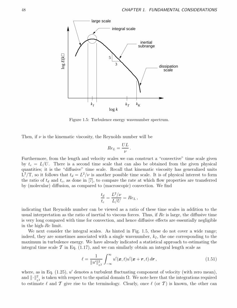
48 CHAPTER 1. FUNDAMENTAL CONSIDERATIONS
log k
log
E(k
)
kKkI kT
large scale
integral scale
inertialsubrange
dissipation scale
5
3
Figure 1.5: Turbulence energy wavenumber spectrum.
Then, if ν is the kinematic viscosity, the Reynolds number will be
ReL =UL
ν.
Furthermore, from the length and velocity scales we can construct a “convective” time scale givenby tc = L/U . There is a second time scale that can also be obtained from the given physicalquantities; it is the “diffusive” time scale. Recall that kinematic viscosity has generalized unitsL2/T, so it follows that td = L2/ν is another possible time scale. It is of physical interest to formthe ratio of td and tc, as done in [7], to compare the rate at which flow properties are transferredby (molecular) diffusion, as compared to (macroscopic) convection. We find
tdtc
=L2/ν
L/U= ReL ,
indicating that Reynolds number can be viewed as a ratio of these time scales in addition to theusual interpretation as the ratio of inertial to viscous forces. Thus, if Re is large, the diffusive timeis very long compared with time for convection, and hence diffusive effects are essentially negligiblein the high-Re limit.
We next consider the integral scales. As hinted in Fig. 1.5, these do not cover a wide range;indeed, they are sometimes associated with a single wavenumber, kI , the one corresponding to themaximum in turbulence energy. We have already indicated a statistical approach to estimating theintegral time scale T in Eq. (1.17), and we can similarly obtain an integral length scale as
ℓ =1
‖u′‖2L2
∫ ∞
−∞
u′(x, t)u′(x + r, t) dr , (1.51)
where, as in Eq. (1.25), u′ denotes a turbulent fluctuating component of velocity (with zero mean),and ‖·‖2
L2is taken with respect to the spatial domain Ω. We note here that the integrations required
to estimate ℓ and T give rise to the terminology. Clearly, once ℓ (or T ) is known, the other can
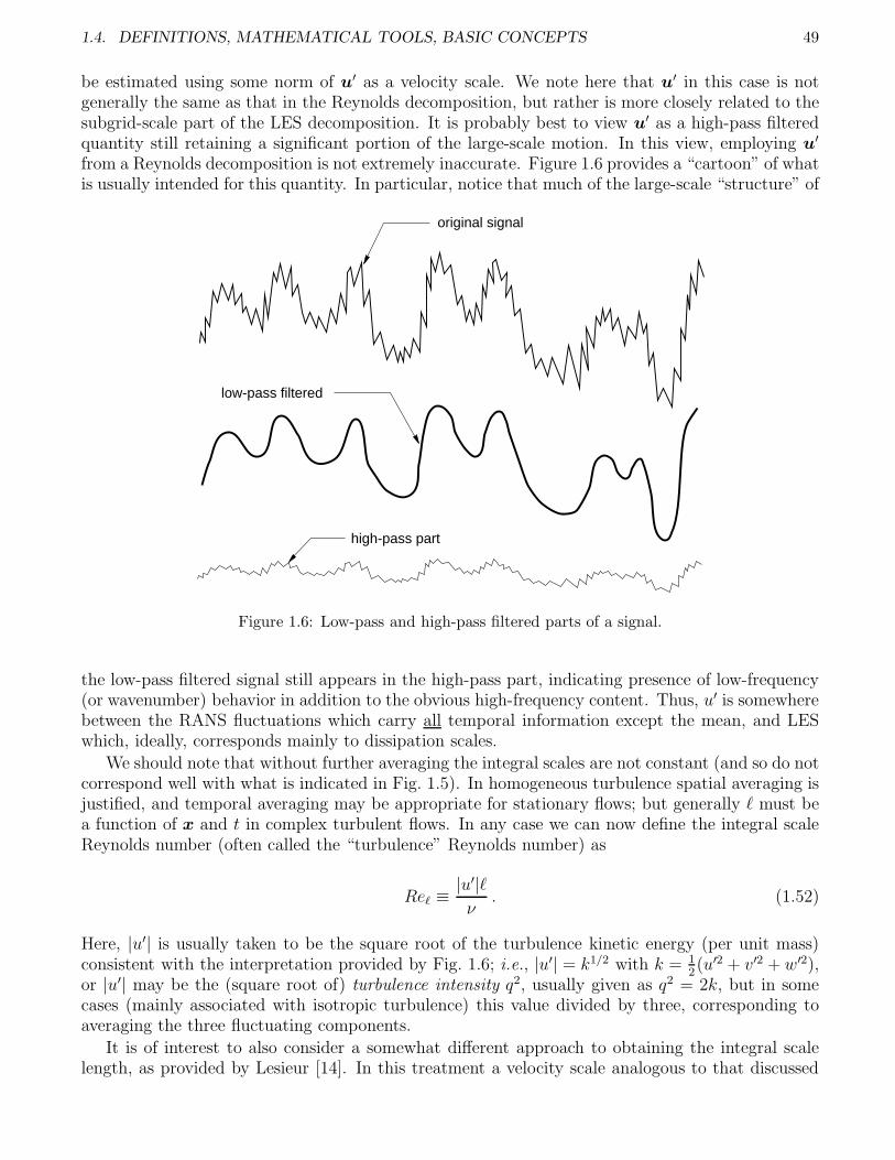
1.4. DEFINITIONS, MATHEMATICAL TOOLS, BASIC CONCEPTS 49
be estimated using some norm of u′ as a velocity scale. We note here that u′ in this case is notgenerally the same as that in the Reynolds decomposition, but rather is more closely related to thesubgrid-scale part of the LES decomposition. It is probably best to view u′ as a high-pass filteredquantity still retaining a significant portion of the large-scale motion. In this view, employing u′
from a Reynolds decomposition is not extremely inaccurate. Figure 1.6 provides a “cartoon” of whatis usually intended for this quantity. In particular, notice that much of the large-scale “structure” of
original signal
low-pass filtered
high-pass part
Figure 1.6: Low-pass and high-pass filtered parts of a signal.
the low-pass filtered signal still appears in the high-pass part, indicating presence of low-frequency(or wavenumber) behavior in addition to the obvious high-frequency content. Thus, u′ is somewherebetween the RANS fluctuations which carry all temporal information except the mean, and LESwhich, ideally, corresponds mainly to dissipation scales.
We should note that without further averaging the integral scales are not constant (and so do notcorrespond well with what is indicated in Fig. 1.5). In homogeneous turbulence spatial averaging isjustified, and temporal averaging may be appropriate for stationary flows; but generally ℓ must bea function of x and t in complex turbulent flows. In any case we can now define the integral scaleReynolds number (often called the “turbulence” Reynolds number) as
Reℓ ≡|u′|ℓ
ν. (1.52)
Here, |u′| is usually taken to be the square root of the turbulence kinetic energy (per unit mass)consistent with the interpretation provided by Fig. 1.6; i.e., |u′| = k1/2 with k = 1
2(u′2 + v′2 + w′2),
or |u′| may be the (square root of) turbulence intensity q2, usually given as q2 = 2k, but in somecases (mainly associated with isotropic turbulence) this value divided by three, corresponding toaveraging the three fluctuating components.
It is of interest to also consider a somewhat different approach to obtaining the integral scalelength, as provided by Lesieur [14]. In this treatment a velocity scale analogous to that discussed

50 CHAPTER 1. FUNDAMENTAL CONSIDERATIONS
above is used, and in conjunction with this, turbulence energy dissipation rate ε, usually given as
ε = 2ν‖S‖2 , (1.53)
is employed to construct a length scale with elements of the strain rate tensor S given earlierin the discussion of Cartesian tensors. In [14] a slightly different definition of ε is used, namely,ε = ν〈ω ·ω〉. In Eq. (1.53) ‖ · ‖ is the usual matrix two norm, and in the preceding formula ω is thevorticity vector. We note that these formulations are equivalent in the sense of norm equivalencesince both S and ω are obtained from rearrangement of ∇U into a sum of symmetric (∼S) andskew-symmetric (∼ω) parts as follows for any arbitrary portion of the velocity field.
∇U =
ux uy uz
vx vy vz
wx wy wz
=1
2
2ux uy + vx uz + wx
vx + uy 2vy vz + wy
wx + uz wy + vy 2wz
+
0 uy − vx uz − wx
vx − uy 0 vz − wy
wx − uz wy − vz 0
.
Also, we observe that the generalized units of ε must be L2/T3. Then it follows that a lengthscale can be constructed as
ℓ =|u′|3
ε. (1.54)
Clearly, this is based entirely on fluctuating velocity still containing some relatively low wavenumberbehavior, and hence, consistent with the physical interpretation of integral scale as inferred fromFig. 1.5. But we remark that if S is decomposed into mean and fluctuating components, ‖S‖ willbe dominated by the latter, implying that ε is mainly a small-scale quantity. We would expect thisbased on our earlier Fourier analysis of the N.–S. equations.
We now derive the length and time scales associated with the Taylor microscale. We begin witha definition for the Taylor microscale length provided in [14]:
λ2 =〈|u′|2〉
〈‖S‖2〉, (1.55)
where we are using the velocity scale discussed previously and are now formally indicating anaveraging process with 〈 · 〉, and again using norm of the strain rate tensor in place of norm ofvorticity since this is more often done (see [7]). Then from Eq. (1.53) (with the factor of twosuppressed, in accord with [14], we obtain the Taylor microscale length expressed as
λ =
[ν〈|u′|2〉
ε
]1/2
. (1.56)
A time scale can be obtained using this length scale and the velocity |u′|, and the Taylor microscaleReynolds number is calculated as
Reλ =|u′|λ
ν. (1.57)
We again note that the Taylor microscale length is roughly consistent with the Kolmogorov inertialsubrange scales.
We now find expressions for the smallest scales of turbulence. These were derived by Kolmogorovunder the assumption that at these scales mainly dissipation would be important, so the only two
1.4. DEFINITIONS, MATHEMATICAL TOOLS, BASIC CONCEPTS 51
physical parameters needed to describe behavior from a dimensional standpoint are viscosity νand dissipation rate ε of turbulence kinetic energy. We will see that combinations of only theseparameters lead to all three of length, time and velocity scales in the dissipation range. Again,recall that the generalized units of kinematic viscosity are L2/T, and those for energy dissipationrate are L2/T3. It follows that a length scale can be obtained by eliminating time between thesetwo sets of units. This can be done by forming the ratio of ν3 with ε, and taking the fourth root ofthe result. Thus, we obtain the Kolmogorov length scale
η =
(ν3
ε
)1/4
. (1.58)
Similarly, a Kolmogorov time scale can be constructed as the square root of the ratio of ν to ε:
τ =(ν
ε
)1/2
. (1.59)
Finally, the Kolmogorov scale velocity is just the ratio of the preceding quantities:
υ = (νε)1/4 . (1.60)
One can readily see that the Reynolds number formed from this length and velocity scale equalsunity, as might be expected on scales where viscous dissipation dominates all other phenomena.
It is of interest to compare some of these various scales. We observe that the length scales andReynolds numbers can be related as follows. First, we can compare the Kolmogorov length scale ηwith the integral scale length ℓ using Eq. (1.58) with Eq. (1.54) solved for ε to write
η ∼
(ν3
|u′|3/ℓ
)1/4
;
thenη
ℓ∼
(ν3
|u′|3ℓ3
)1/4
∼ Re−3/4ℓ ,
orℓ
η∼ Re
3/4ℓ . (1.61)
We have used the ∼ symbol in deriving this result to emphasize that both of Eqs. (1.54) and(1.58) are merely based on dimensional arguments. Nevertheless, Eq. (1.61) has very importantconsequences for computation because it implies that the dissipation scales, which must be resolvedin a DNS of the N.–S. equations, scale like the integral scale Re to the 3/4 power—and this is foronly one direction. Thus, in a 3-D problem the gridding requirements, and hence the computational
work, must scale like Re9/4ℓ for a single time step. As noted by Frisch [80] a typical time step for
numerical stability is of the order of the space step (Courant condition), implying ∼ O(Re3/4ℓ )
required time steps; so a very optimistic (under)estimate of total arithmetic for DNS is ∼Re3ℓ ; for
Re (which, recall, is somewhat larger than Reℓ) of any reasonable size this is still a very formidablecomputation even on modern parallel supercomputers.
We next compare the Taylor and Kolmogorov scales, λ and η, respectively. Again starting withEq. (1.58) we now use Eq. (1.56) with 〈|u′|2〉 replaced with |u′|2 for notational convenience to write
η ∼
(ν3λ2
ν|u′|2
)1/4
∼
(ν2λ2
|u′|2
)1/4
.
52 CHAPTER 1. FUNDAMENTAL CONSIDERATIONS
Thenη
λ∼
(ν2
λ2|u′|2
)1/4
∼ Re−1/2λ ,
orλ
η∼ Re
1/2λ . (1.62)
This shows that length scales in the inertial subrange are a factor of square root of the Taylormicroscale Reynolds number larger than those in the dissipation range. For realistic flow situationsthis tends to be much greater than an order of magnitude.
We can now use results (1.61) and (1.62) to estimate Reλ in terms of Reℓ. First, from thedefinitions of these two Reynolds numbers, Eqs. (1.57) and (1.52), respectively, we have
Reλ
Reℓ=
λ
ℓ. (1.63)
But from (1.61) and (1.62) we have
λ
ℓ∼
Re1/2λ
Re3/4ℓ
=
(λ
ℓ
)1/2
Re1/2ℓ Re
3/4ℓ =
(λ
ℓ
)1/2
Re−1/4ℓ ,
or (λ
ℓ
)1/2
∼ Re−1/4ℓ ⇒
λ
ℓ∼ Re
−1/2ℓ .
Then using Eq. (1.63) for λ/ℓ yields
Reλ ∼ Re1/2ℓ . (1.64)
Finally, again using Eq. (1.62) shows that
λ
η∼ Re
1/4ℓ ,
orη ∼ λRe
−1/4ℓ . (1.65)
Thus, we conclude that
λ ∼ ℓRe−1/2ℓ , and η ∼ λRe
−1/4ℓ , (1.66)
and substitution of the first of these into the second leads back to (1.61), as it must. Finally, notethat for large Reℓ (or ReL), we have η ≪ λ ≪ ℓ.
Taylor’s hypothesis. As noted in Def. 1.110, Taylor’s hypothesis can be employed to deducespatial information about turbulent fluctuations using time series of measurements at a singlepoint, or at a sequence of points at which measurements have not been taken simultaneously. Thepreceding discussions of length and time scales suggest that these can typically be related throughsome velocity scale, and this is what is involved when invoking Taylor’s hypothesis. In particular, asdescribed in [7], measurements of fluctuating velocities are sometimes collected by traversing a probethrough the flow field so rapidly that the nature of the turbulence does not change significantlyduring the measurement process. This permits construction of spatial derivatives of the fluctuatingquantities at an ostensibly fixed time. If the speed of traversal U of the probe is sufficiently high,then a fluctuating velocity signal u′(t) at a fixed location can be identified with fluctuations ata different location a distance x away by substituting t = x/U . This is often termed a “frozen
1.4. DEFINITIONS, MATHEMATICAL TOOLS, BASIC CONCEPTS 53
turbulence” approximation, and it is shown in Hinze [6], among other places, that |u′|/U ≪ 1 musthold for results obtained from Taylor’s hypothesis to be valid.
A somewhat more applicable description of Taylor’s hypothesis is provided by Garde [101].Assume the average flow velocity in the x direction is Uavg . Then turbulent fluctuations u′ observedat a fixed point in space can be approximately interpreted as resulting from a frozen turbulencepattern being convected through the point from elsewhere by a mean flow velocity Uavg . Thissuggests we can relate temporal and spatial derivatives of flow quantities as
∂
∂t= −Uavg
∂
∂x, (1.67)
with the negative sign arising from the fact that a measurement at the current time and spatiallocation corresponds to the frozen pattern that earlier was upstream (negative x) of the current
location. It is noted in [101] that for shear flows√
u′2 ≪ 0.45 must hold, and for isotropic,homogeneous turbulence a value on the order of 10−2 is needed for use of Taylor’s hypothesis toprovide accurate results, an implicit assumption being that Uavg ∼ O(1).
Homogeneous and/or isotropic turbulence. In Def. 1.75 we noted that homogeneous tur-bulence is such that statistics are invariant under spatial translations, and Def. 1.80 implies thatisotropic turbulence is invariant under rotations and reflections. Because rotations and reflectionscan always be constructed as combinations of translations, one might suppose that homogeneityimplies isotropy; but this is not the case. Instead, isotropy is far more restrictive than homogeneity,as we will now describe.
It is important to first note the consequences of homogeneity. The requirement that statisticalproperties remain invariant under arbitrary translations implies, for example, that u′2(x) = u′2(x+r) for any possible vector r ∈ R3 within the domain Ω of the flow field. On the other hand,
homogeneity does not imply that, e.g., u′2(x) = v′2(x), and this provides the distinction betweenhomogeneity and isotropy.
Isotropy requires invariance of statistical quantities under rotations and reflections of the co-ordinate system. Suppose for definiteness that we consider rotating the coordinates through acounter-clockwise angle of 90. Then in this new system, what had been the physical u componentof velocity will now be the v component, and conversely (up to a sign). Thus, if statistics are toremain invariant under rotations it must be that
u′2 = v′2 = w′2 (1.68)
throughout the flow field. But to enforce statistical invariance under arbitrary rotations, beyond(1.68) must be the requirement that derivatives of these quantities in the normal coordinate directionrelative to each also be invariant. This implies that
∂u′2
∂x=
∂v′2
∂y=
∂w′2
∂z(1.69)
must hold.It is thus fairly easy to see that a uniform strain in one direction on homogeneous isotropic
turbulence will destroy the isotropy, but not the homogeneity. On the other hand, few if anyphysical shear flows are uniform, nor are they typically aligned with a single coordinate direction;so generally, introduction of shear (strain) will eliminate both isotropy and homogeneity. That is,real turbulent flows are inhomogeneous and anisotropic. Nevertheless, as is argued in Batchlor [39],the simplifications that can be achieved via assuming homogeneity and isotropy are sufficient topermit some pure analysis of turbulence, and this is considered worthwhile.
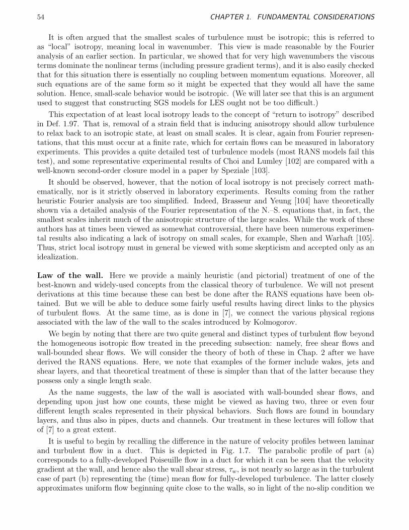
54 CHAPTER 1. FUNDAMENTAL CONSIDERATIONS
It is often argued that the smallest scales of turbulence must be isotropic; this is referred toas “local” isotropy, meaning local in wavenumber. This view is made reasonable by the Fourieranalysis of an earlier section. In particular, we showed that for very high wavenumbers the viscousterms dominate the nonlinear terms (including pressure gradient terms), and it is also easily checkedthat for this situation there is essentially no coupling between momentum equations. Moreover, allsuch equations are of the same form so it might be expected that they would all have the samesolution. Hence, small-scale behavior would be isotropic. (We will later see that this is an argumentused to suggest that constructing SGS models for LES ought not be too difficult.)
This expectation of at least local isotropy leads to the concept of “return to isotropy” describedin Def. 1.97. That is, removal of a strain field that is inducing anisotropy should allow turbulenceto relax back to an isotropic state, at least on small scales. It is clear, again from Fourier represen-tations, that this must occur at a finite rate, which for certain flows can be measured in laboratoryexperiments. This provides a quite detailed test of turbulence models (most RANS models fail thistest), and some representative experimental results of Choi and Lumley [102] are compared with awell-known second-order closure model in a paper by Speziale [103].
It should be observed, however, that the notion of local isotropy is not precisely correct math-ematically, nor is it strictly observed in laboratory experiments. Results coming from the ratherheuristic Fourier analysis are too simplified. Indeed, Brasseur and Yeung [104] have theoreticallyshown via a detailed analysis of the Fourier representation of the N.–S. equations that, in fact, thesmallest scales inherit much of the anisotropic structure of the large scales. While the work of theseauthors has at times been viewed as somewhat controversial, there have been numerous experimen-tal results also indicating a lack of isotropy on small scales, for example, Shen and Warhaft [105].Thus, strict local isotropy must in general be viewed with some skepticism and accepted only as anidealization.
Law of the wall. Here we provide a mainly heuristic (and pictorial) treatment of one of thebest-known and widely-used concepts from the classical theory of turbulence. We will not presentderivations at this time because these can best be done after the RANS equations have been ob-tained. But we will be able to deduce some fairly useful results having direct links to the physicsof turbulent flows. At the same time, as is done in [7], we connect the various physical regionsassociated with the law of the wall to the scales introduced by Kolmogorov.
We begin by noting that there are two quite general and distinct types of turbulent flow beyondthe homogeneous isotropic flow treated in the preceding subsection: namely, free shear flows andwall-bounded shear flows. We will consider the theory of both of these in Chap. 2 after we havederived the RANS equations. Here, we note that examples of the former include wakes, jets andshear layers, and that theoretical treatment of these is simpler than that of the latter because theypossess only a single length scale.
As the name suggests, the law of the wall is asociated with wall-bounded shear flows, anddepending upon just how one counts, these might be viewed as having two, three or even fourdifferent length scales represented in their physical behaviors. Such flows are found in boundarylayers, and thus also in pipes, ducts and channels. Our treatment in these lectures will follow thatof [7] to a great extent.
It is useful to begin by recalling the difference in the nature of velocity profiles between laminarand turbulent flow in a duct. This is depicted in Fig. 1.7. The parabolic profile of part (a)corresponds to a fully-developed Poiseuille flow in a duct for which it can be seen that the velocitygradient at the wall, and hence also the wall shear stress, τw, is not nearly so large as in the turbulentcase of part (b) representing the (time) mean flow for fully-developed turbulence. The latter closelyapproximates uniform flow beginning quite close to the walls, so in light of the no-slip condition we
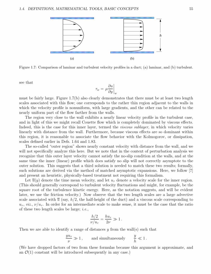
1.4. DEFINITIONS, MATHEMATICAL TOOLS, BASIC CONCEPTS 55
(b)
h
(a)
Figure 1.7: Comparison of laminar and turbulent velocity profiles in a duct; (a) laminar, and (b) turbulent.
see that
τw = µ∂u
∂y
∣∣∣∣w
must be fairly large. Figure 1.7(b) also clearly demonstrates that there must be at least two lengthscales associated with this flow; one corresponds to the rather thin region adjacent to the walls inwhich the velocity profile is nonuniform, with large gradients, and the other can be related to thenearly uniform part of the flow farther from the walls.
The region very close to the wall exhibits a nearly linear velocity profile in the turbulent case,and in light of this we might recall Couette flow which is completely dominated by viscous effects.Indeed, this is the case for this inner layer, termed the viscous sublayer, in which velocity varieslinearly with distance from the wall. Furthermore, because viscous effects are so dominant withinthis region, it is reasonable to associate the flow behavior with the Kolmogorov, or dissipation,scales defined earlier in Defs. 1.64 and 1.83.
The so-called “outer region” shows nearly constant velocity with distance from the wall, and wewill not specifically analyze this here. But we note that in the context of perturbation analysis werecognize that this outer layer velocity cannot satisfy the no-slip condition at the walls, and at thesame time the inner (linear) profile which does satisfy no slip will not correctly asymptote to theouter solution. This suggests that a third solution is needed to match these two results; formally,such solutions are derived via the method of matched asymptotic expansions. Here, we follow [7]and present an heuristic, physically-based treatment not requiring this formalism.
Let u(y) denote the time mean velocity, and let uτ denote a velocity scale for the inner region.(This should generally correspond to turbulent velocity fluctuations and might, for example, be thesquare root of the turbulence kinetic energy. Here, as the notation suggests, and will be evidentlater, we use the friction velocity.) Now observe that the two length scales are a large advectivescale associated with u (say, h/2, the half-height of the duct) and a viscous scale corresponding touτ , viz., ν/uτ . In order for an intermediate scale to make sense, it must be the case that the ratioof these two length scales be large; i.e.,
h/2
ν/uτ
=huτ
2ν≫ 1 .
Then we are able to identify a range of distances y from the wall(s) such that
yuτ
ν≫ 1 , and simultaneously
y
h≪ 1 .
(We have dropped factors of two from these formulas because this argument is approximate, andan O(1) constant will be introduced subsequently in any case.)
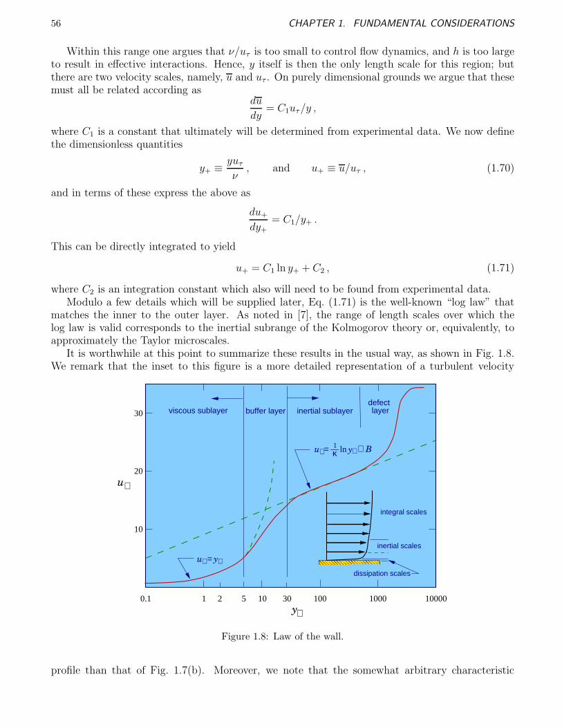
56 CHAPTER 1. FUNDAMENTAL CONSIDERATIONS
Within this range one argues that ν/uτ is too small to control flow dynamics, and h is too largeto result in effective interactions. Hence, y itself is then the only length scale for this region; butthere are two velocity scales, namely, u and uτ . On purely dimensional grounds we argue that thesemust all be related according as
du
dy= C1uτ/y ,
where C1 is a constant that ultimately will be determined from experimental data. We now definethe dimensionless quantities
y+ ≡yuτ
ν, and u+ ≡ u/uτ , (1.70)
and in terms of these express the above as
du+
dy+
= C1/y+ .
This can be directly integrated to yield
u+ = C1 ln y+ + C2 , (1.71)
where C2 is an integration constant which also will need to be found from experimental data.Modulo a few details which will be supplied later, Eq. (1.71) is the well-known “log law” that
matches the inner to the outer layer. As noted in [7], the range of length scales over which thelog law is valid corresponds to the inertial subrange of the Kolmogorov theory or, equivalently, toapproximately the Taylor microscales.
It is worthwhile at this point to summarize these results in the usual way, as shown in Fig. 1.8.We remark that the inset to this figure is a more detailed representation of a turbulent velocity
+
y+
=u+ y+
= ln B__u y+ + +1κ
defectinertial sublayer layer
u
viscous sublayer
0.1 1 52 10 30 100 1000 10000
10
30
20
integral scales
inertial scales
dissipation scales
buffer layer
Figure 1.8: Law of the wall.
profile than that of Fig. 1.7(b). Moreover, we note that the somewhat arbitrary characteristic
1.5. SUMMARY 57
turbulent velocity of the viscous sublayer is usually taken to be the friction velocity as hinted earlierand alluded to in Def. 1.71. This is defined as
uτ =
√τw
ρ. (1.72)
Furthermore, we define in the usual way corresponding to the notation of the figure. The formula inthe figure corresponding to the logarithmic part of the velocity profile contains the usual notationκ for the von Karman constant and B for the integration constant given earlier as C2. In Chap. 2we will discuss these in more detail and, in particular, supply values for them.
We observe that this figure exhibits four different length scales as we hinted earlier might bethe case. The one not previously discussed is usually termed the “buffer layer,” and it (smoothly)connects the the viscous sublayer to the inertial sublayer. As indicated on Fig. 1.8 with dashedlines these two regions match mathematically, but the match is not smooth. Moreover, neitherexperimental nor computational data show the sharp change indicated by the dashed lines. Thebuffer layer might be viewed, physically, as a small range of scales over which inertial and dissipationeffects are nearly balanced, corresponding to the range of wavenumbers in the energy spectrum justbeyond that of the inertial subrange where the decay rate is beginning to increase (recall Fig. 1.5).In addition, the terminology “defect layer” is not universally employed for the outermost (furthestfrom the walls) region. It is suggested by the viewpoint that a turbulent boundary layer might beconsidered to be a turbulent wake with a solid wall on one side. In any case, it is clear from Fig.1.8 that the log law does not hold in this part of a flow; typical length scales are of the order of theintegral scale.
Finally, we note that the importance of the law of the wall in the present era is that it providesan explicit formula for the mean turbulent velocity profile near a solid boundary. With this in handit seems not necessary to employ the fine gridding required to capture behavior on the scales of thebuffer layer and smaller, as is formally necessary in LES; in particular, one can evaluate the log lawformula and use the result as a velocity boundary condition at the outer edge of the buffer layer,or even farther from the wall if extremely coarse gridding is employed. This significantly reducesthe required amount of total arithmetic for simulating wall-bounded shear flows and is widely usedboth in RANS methods and in LES. But it is important to recall the assumption that led to thelog-law result, viz., fully-developed flow. As a consequence, the simple law of the wall describedhere is not valid for nonself-similar boundary layers, and furthermore cannot be used accuratelyin the presence of flow separation. There have, however, been numerous attempts to extend thelaw of the wall to other flow situations beginning already with Tennekes and Lumley [7], and someof these have been at least moderately successful. But treatment of these is beyond the intendedscope of these lectures, and the reader is referred to the extant literature.
1.5 Summary
In this introductory chapter we have begun by first attempting to provide some heuristic viewsof turbulence, an historical overview of its study and the progress to date, to some extent con-trasting the classical, statistical view of turbulence as a random phenomenon with the modern,deterministic viewpoint. We next included an extensive glossary of terms associated with turbu-lence, many of which will be used repeatedly as we proceed through the following lectures. Then,as further preparation for these, we presented fairly detailed discussions of numerous mathematicaland physical ideas that are of a fundamental nature and thus will be of use independent of whetherwe are considering the classical or modern view of turbulence. These included several alternativedecompositions of flow variables, Fourier analysis of the N.–S. equations, length and time scales ofturbulence, and the law of the wall.
58 CHAPTER 1. FUNDAMENTAL CONSIDERATIONS
We again emphasize that it is now almost universally accepted that the N.–S. equations arecapable of producing turbulent solutions. Moreover, such solutions obtained via DNS agree ex-ceptionally well with experimental observations within the range of Reynolds numbers currentlyaccessible by this technique. This suggests that independent of what form of modeling might be at-tempted, tests of model results and/or analysis of model structure must include direct comparisonswith the N.–S. equations and their solutions.
Chapter 2
Statistical Analysis and Modeling of
Turbulence
Statistical analyses of turbulence have been employed from the beginning, certainly already inReynolds’ 1894 paper [16], but at least implicitly in the earlier work of Boussinesq [15] in 1877. Theworks of Reynolds, Prandtl, Taylor and others emphasized the perceived randomness of turbulentflows with the implication that statistical approaches were the only possibility for analysis, andthis view was dominant during the early years of development of turbulence modeling proceduresnecessitated by averaging the nonlinear Navier–Stokes (N.–S.) equations.
In a sense, modeling began with the work of Boussinesq cited above, but in the absence of theReynolds decomposition formalism. Prandtl’s mixing length theory represents the first turbulencemodel in a more modern sense; in particular, it attempts to estimate values of eddy viscosity,introduced by Boussinesq, to close the Reynolds-averaged Navier–Stokes (RANS) equations. It issometimes claimed that Kolmogorov [106] already by 1942 had introduced the ideas underlying k−εmodels that we will treat in the sequel, and similar ideas were proposed later by Rotta [107] in 1951.But Jones and Launder [108] introduced the basic form of these models that has been studied to thepresent. In addition, Launder et al. [109] presented the form of so-called second-order, or second-moment closures, also called Reynolds stress models, that until rather recently received considerableattention.
In this chapter we begin by deriving the RANS equations, and then discuss a number of math-ematical consequences that are independent of modeling. Following this we consider some detailsof a number of specific, widely-used models including Prandtl’s mixing length, k−ε models, eddyviscosity transport and the basics of second-order closures. We then provide a section in which theKolmogorov theories are discussed. These also are statistical, but they do not rely on a Reynoldsdecomposition, and until only recently little effort had been expended in attempts to make directuse of them in modeling. We remark that this was probably at least in part due to the fact thatthis theory did not seem to provide anything of use for typical RANS approaches that, as we willsee, usually require construction of an eddy viscosity.
2.1 The Reynolds-Averaged Navier–Stokes Equations
In this section we begin by employing the Reynolds decomposition, Eq. (1.25), to derive the RANSequations. We then obtain related results for vorticity transport and examine the relationshipbetween vortex stretching and Reynolds stresses. We follow this with analyses of attempts toinclude time dependence in the RANS equations, and in particular consider a currently-popularprocedure termed unsteady RANS (URANS). We then provide a fairly detailed analysis of the
59
60 CHAPTER 2. STATISTICAL ANALYSIS AND MODELING OF TURBULENCE
inherent difficulties of RANS approaches in general, both with respect to formal mathematics, andwith respect to physics. Finally, we present descriptions and comparisons of some of the morewidely-implemented RANS procedures.
2.1.1 Derivation of the RANS equations
The starting point for this derivation is, of course, the N.–S. equations,
∇ · U = 0 , (2.1a)
Ut + U · ∇U = −∇P + ν∆U , (2.1b)
given earlier in Eqs. (1.1), and written here without the body-force term. We next recall Eq. (1.25)for the Reynolds decomposition and substitute this into the first of the above equations:
∇ · U = ∇ · (u + u′) = ∇ · u + ∇ · u′ = 0 . (2.2)
Then averaging this equation results in
∇ · u + ∇ · u′ = 0 , (2.3)
and from Eq. (1.26) we deduce that∇ · u = 0 . (2.4)
Then it follows from the far right-hand side of Eq. (2.2) that
∇ · u′ = 0 (2.5)
also holds.We remark that if the averaging performed in Eq. (2.3) had been omitted, we might conclude
that only∇ · u = −∇ · u′
is required to satisfy the divergence-free constraint of the overall velocity field. But we should recallthat the Galerkin form of the N.–S. equations implies that the divergence-free condition must holdon a mode-by-mode basis (recall Eq. (1.41)), and this would be contradicted by the above.
We next consider Eqs. (2.1b). We begin by substituting Eq. (1.25) for each entry of U , with ananalogous expression for P , to obtain
(u + u′)t + (u + u′) · ∇ (u + u′) = −∇ (p + p′) + ν∆ (u + u′) .
Now recall that u is independent of t, by definition, so the first term in this expression is identicallyzero. Then upon expansion of the dot product on the left-hand side we have
u′
t + u · ∇u + u · ∇u′ + u′ · ∇u + u′ · ∇u′ = −∇ (p + p′) + ν∆ (u + u′) .
Next, just as we did with the continuity equation, we time average the entire equation. Thisresults in
u′
t + u · ∇u + u · ∇u′ + u′ · ∇u + u′ · ∇u′ = −∇(p + p′) + ν∆(u + u′) . (2.6)
Here, we have already commuted time averaging and spatial differentiation in the linear terms onthe right-hand side. Proof of validity of this is trivial. We next commute temporal averaging anddifferentiation in the first term on the left-hand side, and use the second of Eqs. (1.26) to concludethat
u′
t =(u′
)t≡ 0 . (2.7)
2.1. THE REYNOLDS-AVERAGED NAVIER–STOKES EQUATIONS 61
We leave formal proof of validity of this, under the assumption that u′ ∈C1(R+) with respect totime as an exercise for the reader.
Using Eqs. (1.26) in the right-hand side of (2.6) and (2.7) on the left-hand side leaves
u · ∇u + u · ∇u′ + u′ · ∇u + u′ · ∇u′ = −∇p + ν∆u . (2.8)
We now consider the details of u · ∇u′. We have, by definition of the time average, that
u · ∇u′ = limT→∞
1
T
∫ T
0
u · ∇u′ dt
= u ·
[lim
T→∞
1
T
∫ T
0
∇u′ dt
]
= u · ∇
[lim
T→∞
1
T
∫ T
0
u′ dt
]
= u · ∇u′
= 0 .
The second equality follows because u is independent of t. Similarly, the third occurs because ∇,as an operator, is also independent of time, and the final equality arises from application of thesecond equation in (1.26). A similar analysis can be carried out for u′ · ∇u, with the same resultholding. Thus, Eq. (2.8) becomes
u · ∇u + u′ · ∇u′ = −∇p + ν∆u .
We next observe that by the divergence-free conditions Eqs. (2.4) and (2.5), the terms on the
left-hand side of the above can be expressed as ∇·u2 and ∇·u′2, respectively, where u2 is shorthandnotation for (u, v, w)T (u, v, w). We leave demonstration of this as an exercise. Then it easily followsthat
∇·u2 = ∇·u2 = ∇·u2 ,
and∇·u′2 = ∇·u′2 .
(Again, supplying detailed arguments is left to the reader.) As a consequence of these identities wecan now write Eq. (2.8) as
∇·u2 + ∇·u′2 = −∇p + ν∆u , (2.9)
the Reynolds-averaged Navier–Stokes equations. It is clear that this vector equation contains farmore unknowns than equations; that is, the second term on the left-hand side does not possessan equation for any of its six independent components to be described in more detail below. Thisconstitutes our first direct encounter with the so-called “turbulence closure problem” which has ledto extensive modeling efforts from the early 20th Century to the present day.
We note that there are numerous formulations for the RANS equations, with no particularnotation being completely standard. We present a few of the more common ones here. We begin
by noting that u′2 is usually called the Reynolds stress tensor although a check of dimensions willshow that it is not actually a stress; it must be multiplied by density ρ, as done consistently in [7],in order to have dimensions corresponding to the terminology. (On the other hand, since ρ ≡ const.we might set it to unity, thus obtaining implicit dimensional correctness. Moreover, because we
62 CHAPTER 2. STATISTICAL ANALYSIS AND MODELING OF TURBULENCE
typically employ kinematic viscosity, there is an implied division by ρ in any case.) The matrixrepresentation of this tensor is the following:
u′2 =
u′2 u′v′ u′w′
u′v′ v′2 v′w′
u′w′ v′w′ w′2
. (2.10)
In addition, in Cartesian tensor notation this is often denoted simply as R with components some-times denoted both by Rij and rij and expressed as
R =
u′1u
′1 u′
1u′2 u′
1u′3
u′1u
′2 u′
2u′2 u′
2u′3
u′1u
′3 u′
2u′3 u′
3u′3
. (2.11)
In this context the individual components are often also denoted τij , especially after multiplicationby ρ as described above. We will not use this notation herein as we prefer to employ this forcomponents of the complete (undecomposed) stress tensor. Finally, the functional tensor notationR(u′, u′) will sometimes be found. Note that this usually contains the divergence operator as wellas the Reynolds stress tensor to simplify the notation; that is
R(u′, u′) = ∇ ·
u′2 u′v′ u′w′
u′v′ v′2 v′w′
u′w′ v′w′ w′2
.
Thus, Eq. (2.9) might be written in any one of the following alternative (and equivalent) ways:
∇·u2 = −∇p + ν∆u − R(u′, u′) , (2.12a)
∂
∂xj
uiuj = −∂p
∂xi
+ ν∂2ui
∂xj∂xj
−∂
∂xj
u′iu
′j , i = 1, 2, 3 , (2.12b)
∂
∂xjuiuj = −
∂p
∂xi+ ν
∂2ui
∂xj∂xj−
∂Rij
∂xj, i = 1, 2, 3 , (2.12c)
or with Rij in Eq. (2.12c) replaced with either rij or τij . We will mainly employ the first two ofthese notations, or Eq. (2.9), itself, in the sequel.
Finally, as we have already noted, it is common to ignor the fact that u is independent of timeand write, e.g.,
ut + ∇·u2 = −∇p + ν∆u − R(u′, u′) , (2.13)
or in Cartesian tensor notation,
ui,t +∂
∂xj
uiuj = −∂p
∂xi
+ ν∂2ui
∂xj∂xj
−∂
∂xj
u′iu
′j , i = 1, 2, 3 . (2.14)
We will examine this in more detail in the following section.
2.1. THE REYNOLDS-AVERAGED NAVIER–STOKES EQUATIONS 63
2.1.2 Time-dependent RANS equations
In essentially all modern practical formulations of the RANS equations the time derivative term∂u/∂t is included, despite the fact that u = u(x) only is independent of time. In this section webriefly discuss two of the widely-used arguments justifying retention of this term. The first of thesecomes from an appeal to ergodicity of turbulent flows while the second is associated with time scalesactually needed to obtain reasonably accurate averages. We consider some details of each of theseand present consequences that follow from these arguments.
Appeal to Ergodicity
Recall from Def. 1.3 that the ergodic hypothesis implies “time averaging is equal to ensembleaveraging.” There are several precise statements of this, and the reader is referred to Frisch [80] formore details. Here, we first indicate how this might be employed, and then return to some of thedetails.
We first recall from Chap. 1 that the ensemble average of N realizations of a variable u(x, t),say
〈u(x, t)〉 =1
N
N∑
i=1
u(i)(x, t) ,
is formally time dependent. Consequently, we might write the ensemble-averaged N.–S. equationsas
〈U〉t + 〈U〉·∇〈U〉 = −∇〈P 〉 + ν∆〈U 〉 − R(u′, u′) , (2.15)
with the components of R now computed with ensemble averaging.This form was often employed in early analyses of turbulence (see, e.g., Batchelor [39]), but
more recently it has sometimes been used in conjunction with the ergodic hypothesis to justifythe form of the RANS equations given in Eq. (2.13). That is, if retaining the time dependence inensemble-averaged equations is valid, and ensemble averaging is equivalent to time averaging, thenit follows that
ut + u·∇u = −∇p + ν∆u − R(u′, u′)
is a valid equation to consider.There is, however, a basic flaw in this argument, and this arises from not recalling the hypotheses
required in the ergodic theorems. There are two basic ones. The first is stationarity of the flow.Bradshaw [110] comments on the importance of this in turbulent flow data. Indeed, most (butnot all) turbulent flows considered in practice are stationary. The second hypothesis is that theformal limit T → ∞ be observed in the time-averaging process just as implied by the definition.The consequence of this is that formal time dependence of the ensemble-averaged equations cannotbe used to deduce time dependence of the usual time-averaged equations, but rather preciselythe opposite must hold—solutions to the ensemble-averaged equations, themselves, are not timedependent. In fact, this can be inferred also from the discussions in [80] although it is not explicitlystated there. (But note that this does not invalidate use of ensemble averages to obtain time-dependent data. It simply negates use of the ergodic hypothesis.)
Use of Multiple Time Scales
Probably the most commonly-used justification for retaining the time-derivative operator in theRANS equations comes from arguments associated with multiple time scales. These arguments areusually rather heuristic, but Wilcox [98] provides a particularly good treatment of this, and we willfollow this, to some extent, in the present discussions.
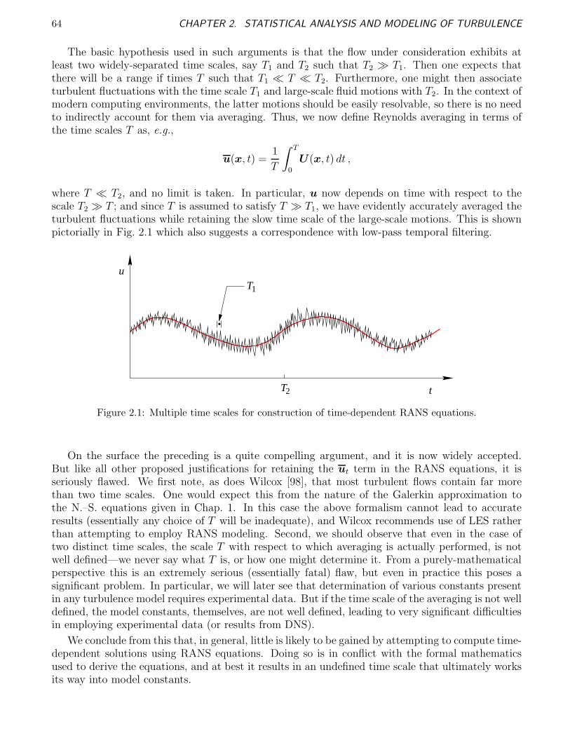
64 CHAPTER 2. STATISTICAL ANALYSIS AND MODELING OF TURBULENCE
The basic hypothesis used in such arguments is that the flow under consideration exhibits atleast two widely-separated time scales, say T1 and T2 such that T2 ≫ T1. Then one expects thatthere will be a range if times T such that T1 ≪ T ≪ T2. Furthermore, one might then associateturbulent fluctuations with the time scale T1 and large-scale fluid motions with T2. In the context ofmodern computing environments, the latter motions should be easily resolvable, so there is no needto indirectly account for them via averaging. Thus, we now define Reynolds averaging in terms ofthe time scales T as, e.g.,
u(x, t) =1
T
∫ T
0
U(x, t) dt ,
where T ≪ T2, and no limit is taken. In particular, u now depends on time with respect to thescale T2 ≫ T ; and since T is assumed to satisfy T ≫ T1, we have evidently accurately averaged theturbulent fluctuations while retaining the slow time scale of the large-scale motions. This is shownpictorially in Fig. 2.1 which also suggests a correspondence with low-pass temporal filtering.
T t
u
1T
2
.
Figure 2.1: Multiple time scales for construction of time-dependent RANS equations.
On the surface the preceding is a quite compelling argument, and it is now widely accepted.But like all other proposed justifications for retaining the ut term in the RANS equations, it isseriously flawed. We first note, as does Wilcox [98], that most turbulent flows contain far morethan two time scales. One would expect this from the nature of the Galerkin approximation tothe N.–S. equations given in Chap. 1. In this case the above formalism cannot lead to accurateresults (essentially any choice of T will be inadequate), and Wilcox recommends use of LES ratherthan attempting to employ RANS modeling. Second, we should observe that even in the case oftwo distinct time scales, the scale T with respect to which averaging is actually performed, is notwell defined—we never say what T is, or how one might determine it. From a purely-mathematicalperspective this is an extremely serious (essentially fatal) flaw, but even in practice this poses asignificant problem. In particular, we will later see that determination of various constants presentin any turbulence model requires experimental data. But if the time scale of the averaging is not welldefined, the model constants, themselves, are not well defined, leading to very significant difficultiesin employing experimental data (or results from DNS).
We conclude from this that, in general, little is likely to be gained by attempting to compute time-dependent solutions using RANS equations. Doing so is in conflict with the formal mathematicsused to derive the equations, and at best it results in an undefined time scale that ultimately worksits way into model constants.
2.1. THE REYNOLDS-AVERAGED NAVIER–STOKES EQUATIONS 65
2.1.3 Importance of vorticity and vortex stretching to turbulence
We have earlier observed that turbulence is inherently three dimensional; indeed, even in flows thatare at least nearly 2D on large scales, it is observed in laboratory experiments that small-scalefluctuations are generally three dimensional. Furthermore, it is widely argued that turbulence,itself, is intimately connected with vorticity. References as otherwise widely disparate as Tennekesand Lumley [7] and Tsinober [3] make this same claim—albeit for different reasons and backedby different supporting arguments. Tennekes and Lumley argue that turbulence must be 3D onthe basis of demonstrating a relationship between vortex stretching and production of Reynoldsstresses, and the fact that vortex stretching can only occur in 3D; hence, Reynolds stresses can onlybe generated in 3D flows. Moreover, they argue that vortex stretching is the physical mechanismleading to the hypothesized energy cascade from large to small scales. On the other hand, Tsinober[3] notes first that this cascade is not exactly what happens and second that it is in fact vortexcompression—not stretching—that would result in energy transfer to smaller scales. But in addition,he emphasizes that strain rate is equally as important as vorticity in the context of creation andmaintenance of turbulence.
In this section we first present a somewhat different view of vorticity and its importance influid flow, generally. We then outline arguments provided in [7], but balanced by those in [3] andinterpreted in light of the viewpoint given here.
What Is Vorticity, and How Important Is It—Really?
Vorticity and its study have been extremely important topics in almost any fluid dynamicscourse for the past century, and as already noted vorticity is considered to be a key ingredient ofa turbulent flow. But what, exactly, is vorticity? It certainly is not a property of the fluid; butmoreover, it is not a directly-measurable physical property of the flow. In fact, vorticity is nothingbut a mathematical definition—the curl of the velocity field:
ω ≡ ∇×U . (2.16)
Thus, mathematical vorticity is constructed from gradients of the physical flow property velocity,and these gradients are calculated from measured velocity fields, leading to a rather indirect deter-mination of vorticity. Furthermore, the same is true of strain rates, and this should be of no surprisebecause both rotation (essentially one half of the vorticity) and strain rate arise in a straightforwarddecomposition of the velocity gradient tensor (the Jacobian matrix of the velocity field) as is wellknown and is shown in Chap. 1.
What is clear from this is that the fundamental physical quantity is the set of velocity gra-dients; vorticity and strain rates are derived quantities. This is not, however, intended to implythat they are unimportant, or that they are not useful, but rather that they have possibly beenoveremphasized. Moreover, vorticity does not occur naturally in the N.–S. equations (or even intheir derivation), and while strain rate is an important element of the derivation it does not, perse, appear in the final form of the equations unless variable transport properties are considered.Thus, especially in the case of vorticity, an overemphasis of its use in deducing flow behaviors can,potentially, result in misleading notions.
Relationship between Vorticity and Reynolds Stress
Here we will closely follow the treatment found in [7] to demonstrate the connection of vorticityto Reynolds stress, and thus to turbulence in the context of a Reynolds-averaged Navier–Stokes

66 CHAPTER 2. STATISTICAL ANALYSIS AND MODELING OF TURBULENCE
interpretation. As in that reference, we begin by writing the N.–S. equations in terms of Cartesiantensor notation given in Eqs. (1.30):
∂ui
∂t+ uj
∂ui
∂xj= −
∂p
∂xi+ ν
∂2ui
∂xj∂xj, i = 1, 2, 3 . (2.17)
We now express the advective term as
uj∂ui
∂xj= uj
(∂ui
∂xj−
∂uj
∂xi
)+ uj
∂uj
∂xi
= −ǫijkujωk +∂
∂xi
(1
2ujuj
),
and substitute this into Eq. (2.17) to obtain
∂ui
∂t+
1
2
∂
∂xi(ujuj) = −
∂p
∂xi+ ǫijkujωk + ν
∂2ui
∂xj∂xj, (2.18)
We next introduce the Reynolds decompositions
ui = ui + u′i , ωi = ωi + ω′
i , p = p + p′ , i = 1, 2, 3 ,
and use these in Eq. (2.18) followed by averaging of the result to arrive at
1
2
∂
∂xi
(ujuj) = −∂p
∂xi
−1
2
∂
∂xi
(u′
ju′j
)+ ǫijk
(ujωk + u′
jω′k
)+ ν
∂2ui
∂xj∂xj
,
or1
2
∂
∂xi
(u′
ju′j
)− ǫijku′
jω′k = −
∂
∂xi
(p +
1
2ujuj
)+ ǫijkujωk + ν
∂2ui
∂xj∂xj. (2.19)
Here, we have expressed the fluctuating quantities related to Reynolds stresses in terms of meanquantities, including mean vorticity, thus emphasizing the importance of vorticity in generation ofthe Reynolds stresses.
There are, however, two serious flaws in this argument. The first is that introduction of vorticityinto the N.–S. equations as done here is contrived and artificial; it in no way reflects any actualphysics. (It was obtained by adding zero to the momentum equations.) But the second is moredamaging, for even if introduction of vorticity could be argued on physical grounds, there is nojustification for the implicit assumption that the Reynolds stresses are turbulence. In the first place,they are merely artifacts of having averaged the N.–S. equations—again, simply a mathematicaloperation; but beyond this is the fact that, formally, Reynolds stresses could be constructed for anystationary time-dependent flow, whether or not it happens to be turbulent. Finally, the Reynoldsstresses, themselves, are time-averaged quantities and hence independent of time, and beyond thisis the fact that only the normal stresses actually appear in the formulation. It is thus difficult torationalize a direct equivalence between turbulence, which is characterized as always being timedependent, and a simple velocity correlation that by definition does not depend on time.
Vortex Stretching and Turbulence
As mentioned earlier, one of the proposed mechanisms for transferring energy from large tosmall scales is via vortex stretching. The basic physical idea is that a vortex tube subjected tostrain from local velocity gradients of the surrounding flow field will be stretched, thus shrinking
2.1. THE REYNOLDS-AVERAGED NAVIER–STOKES EQUATIONS 67
its diameter. Then the energy associated with this vortex is acting at smaller length scales (andhigher wavenumbers). For the moment we will assume validity of this argument and examinethe mathematical representation of the N.–S. equations to identify terms able to generate thisbehavior. In particular, we will be seeking terms involving interactions of strain rate and vorticityin the context of the vorticity equation.
The 2-D vorticity equation. We first consider the two-dimensional case. If one begins withthe 2-D N.–S. equations and computes the curl of these, the result is the 2-D vorticity transportequation,
ωt + U · ∇ω = ν∆ω . (2.20)
Observe that in 2D only the third component of the vorticity vector is nonzero, and we denote thissimply as the scalar ω.
If we now recall that components of the strain rate are of the form, e.g.,
S12 =1
2
(∂u2
∂x1
+∂u1
∂x2
)=
1
2(vx + uy) ,
we readily see that Eq. (2.20) contains no such factors. (Recall that they do appear in the formalderivation of the N.–S. equations but disappear via the divergence-free constraint in the case ofconstant-viscosity flows even for these more fundamental equations.) From this it is concluded thatturbulence cannot be 2D. That is, there is no mechanism in 2D to cause vortex stretching in thevorticity transport equation, and hence no physics to facilitate the energy cascade.
The 3-D vorticity equation. We now provide a more detailed analysis for the 3-D case. Justas in 2D we take the curl of the momentum equations (2.1b), but in contrast to the 2-D case theresult will now be a vector. Formally, we write
∇×[U t + U ·∇U ] = −∇×∇P + ∇×∆U .
Since the curl of a gradient is identically zero (under mild smoothness conditions) as is easily checked,the first term on the right-hand side is zero, as in 2D. Furthermore, assuming some smoothness, wecommute ∇× and ∂/∂t, and ∇× and ∆. Then the above becomes
(∇×U)t + ∇× (U ·∇U) = ν∆(∇×U) ,
orωt + ∇× (U ·∇U) = ν∆ω ,
where ω ≡ (ω1, ω2, ω3)T is the 3-D vorticity vector.
We now need to consider the curl of the advective terms in more detail. We have
∇× (U ·∇U) = (∇×U)·∇U + U ·(∇×∇U)
= (∇×U)·∇U + U ·∇(∇× U)
= ω ·∇U + U ·∇ω .
Then the 3-D vorticity transport equation can be expressed as
ωt + U ·∇ω = −ω ·∇U + ν∆ω , (2.21)
which is of the same general form found for the 2-D case, Eq. (2.20), except for the term −ω ·∇U
on the right-hand side. Now recall, as we have shown in Chap. 1, that ∇U can be decomposed asthe sum of strain rate and rotation tensors. In particular, this extra term appearing in the 3-D case
68 CHAPTER 2. STATISTICAL ANALYSIS AND MODELING OF TURBULENCE
is associated with the interaction of vorticity and and the velocity gradient tensor (which containsstrain rate—but also vorticity), and is called the “vortex-stretching” term.
It is important to recognize, however, that while vorticity can be a useful tool in studying fluidflow, its overemphasis can be misleading, as we have already suggested. In the present contextthere has been a tendency to identify existence of vorticity with actual vortices, or “eddies,” andarrive at a cartoon of turbulence in which these hypothesized eddies and their behaviors are usedto explain the nature of turbulence. The cascade of turbulent energy from large to small scales isa prime example of this. In particular, we have contrived a theory of the 3-D vorticity equationthat supports such a cascade when it is now known that the simple idea of vortex stretching andsubsequent breaking into yet smaller vortices (eddies) is not an accurate picture of actual physics.Moreover, especially in wall-bounded shear flows it has been found that as much as one third of theenergy cascaded to small scales is “back scattered” up to the large scales. But in addition to this, thesimple eddy cartoon of a turbulent flow is hardly an accurate representation in any circumstance.At any given instant the fraction of the volume of a turbulent flow actually occupied by eddies canbe rather small. This, of course, does not imply that the vorticity is zero nearly everywhere butrather serves to emphasize that constructing a physical theory based on this cartoon of vorticaleddies may be ill advised. Finally, we observe that there is a logical inconsistency in attempting toview strain rate as the cause of vortex stretching. Namely, vorticity and strain rate are somewhatartificially contrived contributions to the velocity gradient tensor. Hence, they occur simultaneously,thus removing the ability of one of them the “cause” the other.
2.1.4 Some general problems with RANS formulations
In this section we discuss several specific problems that are inherent in RANS formulations inde-pendent of details of any specific model. These are: i) the time-averaging process, ii) the Reynoldsdecomposition, iii) the generic form of the RANS equations and iv) general inequality of time-averaged N.–S. solutions and RANS solutions.
Effects of Time Averaging
We will here restrict attention to time averaging since this is essentially always employed inpractical RANS formulations, and we begin by noting that averaging intrinsically results in a loss ofinformation. Indeed, this is the purpose of averaging—to strip away “non-essential” details leavingonly the core information. Figure 2.2 displays this idea in a pictorial way, and with respect tothis it is worthwhile to recall Reynolds’ [16] proposal that it would be impossible to understandturbulence in detail, and it would thus be more useful to consider only statistical properties of aturbulent flow.
There are at least two fundamental flaws with this viewpoint in the context of fluid physics. Thefirst is that in many flow situations details are, in fact, quite essential. An important example of this,which we will consider again later, is turbulent combustion: the small-scale flow field fluctuationscan interact with the chemical kinetics leading to significant changes in reaction rates, temperatureand species concentrations. These effects cannot be ignored if accurate predictions are desired.
But there is a second difficulty that arises from averaging, or from use of statistical characteri-zations in general. It is that the mapping
physics −→ statistics
is many to one. That is, the same statistics (at least at the level of only the first few moments,as considered in RANS formulations) can be generated from many different physical flows. This iseasy to imagine simply be replacing the erratic signal shown in Fig. 2.2(a) with any periodic signal
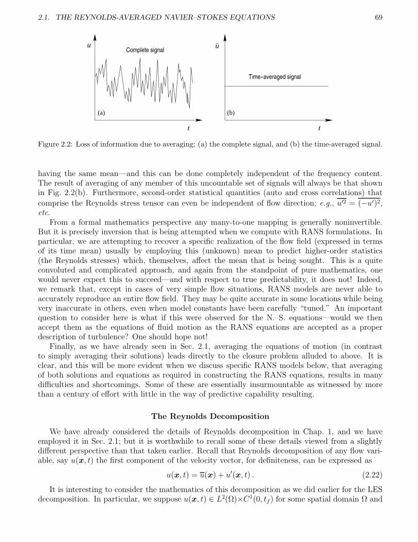
2.1. THE REYNOLDS-AVERAGED NAVIER–STOKES EQUATIONS 69
(a)
Time−averaged signal
t
uComplete signal
u
t
(b)
Figure 2.2: Loss of information due to averaging; (a) the complete signal, and (b) the time-averaged signal.
having the same mean—and this can be done completely independent of the frequency content.The result of averaging of any member of this uncountable set of signals will always be that shownin Fig. 2.2(b). Furthermore, second-order statistical quantities (auto and cross correlations) that
comprise the Reynolds stress tensor can even be independent of flow direction; e.g., u′2 = (−u′)2,etc.
From a formal mathematics perspective any many-to-one mapping is generally noninvertible.But it is precisely inversion that is being attempted when we compute with RANS formulations. Inparticular, we are attempting to recover a specific realization of the flow field (expressed in termsof its time mean) usually by employing this (unknown) mean to predict higher-order statistics(the Reynolds stresses) which, themselves, affect the mean that is being sought. This is a quiteconvoluted and complicated approach, and again from the standpoint of pure mathematics, onewould never expect this to succeed—and with respect to true predictability, it does not! Indeed,we remark that, except in cases of very simple flow situations, RANS models are never able toaccurately reproduce an entire flow field. They may be quite accurate in some locations while beingvery inaccurate in others, even when model constants have been carefully “tuned.” An importantquestion to consider here is what if this were observed for the N.–S. equations—would we thenaccept them as the equations of fluid motion as the RANS equations are accepted as a properdescription of turbulence? One should hope not!
Finally, as we have already seen in Sec. 2.1, averaging the equations of motion (in contrastto simply averaging their solutions) leads directly to the closure problem alluded to above. It isclear, and this will be more evident when we discuss specific RANS models below, that averagingof both solutions and equations as required in constructing the RANS equations, results in manydifficulties and shortcomings. Some of these are essentially insurmountable as witnessed by morethan a century of effort with little in the way of predictive capability resulting.
The Reynolds Decomposition
We have already considered the details of Reynolds decomposition in Chap. 1, and we haveemployed it in Sec. 2.1; but it is worthwhile to recall some of these details viewed from a slightlydifferent perspective than that taken earlier. Recall that Reynolds decomposition of any flow vari-able, say u(x, t) the first component of the velocity vector, for definiteness, can be expressed as
u(x, t) = u(x) + u′(x, t) . (2.22)
It is interesting to consider the mathematics of this decomposition as we did earlier for the LESdecomposition. In particular, we suppose u(x, t) ∈ L2(Ω)×C1(0, tf) for some spatial domain Ω and
70 CHAPTER 2. STATISTICAL ANALYSIS AND MODELING OF TURBULENCE
time interval (0, tf ], possibly with tf → ∞. Then, as done in Chap. 1, we can express u(x, t) as theFourier series
u(x, t) =
∞∑
|k|≥0
ak(t)ϕk(x) .
We now time average this representation:
limT→∞
1
T
∫ T
0
u(x, t) dt = limT→∞
1
T
∫ T
0
∑
k
ak(t)ϕk(x) dt
=∑
k
(lim
T→∞
1
T
∫ T
0
ak(t) dt
)ϕk
=∑
k
akϕk(x) .
It then follows from (2.22) that
u′(x, t) =∑
k
(ak(t) − ak) ϕk(x) . (2.23)
Now if we associate ak with the “dc” part of the original signal u(x, t), as would commonlybe done in signal processing analyses, we see that u′(x, t) contains all other (temporal) modes ofthe Fourier representation and, moreover, contains all spatial wavenumbers. That is, in general, u′
represents all of the solution except the zeroth temporal modes, and as a consequence we shouldexpect that it would be quite difficult to model. But, at least in principle, this is precisely whatmust be modeled in RANS formulations; that is, essentially the entire solution must be modeled!
Generic Form of RANS Equations—Absence of Interactions on Small Scales
The above implied difficulties led, from the beginning, to modeling of flow statistics (the Reynoldsstresses, e.g., u′v′) rather than flow physics (u′, v′, etc.), and this essentially precludes any possibil-ity for resolving short-time/small-length scale interactions between turbulence and other physicalphenomena. To begin with, the quantities actually modeled (e.g., u′v′) have already been averagedover a time considered long compared with time scales of the turbulent fluctuating quantities them-selves. In fact, as we have discussed earlier, for this averaging to be well defined it is necessary thatthe averaging time approach infinity. Thus, u′v′ for example, is not even time dependent. At thesame time, in typical computations the spatial scales are chosen to be small enough for resolution oflarge-scale behavior, but little more. Thus, in RANS formalisms, both spatial and temporal scaleson which interactions would occur are absent from the models.
There are numerous physical situations in which such an approach cannot succeed. We willdescribe two of these here. It is well known (see Warhaft [111] and references therein) that passivescalars tend to exhibit a greater degree of intermittency (in the sense related to flatness, as discussedby Frisch [80]) than does the turbulent flow in which they are being carried. So consider a fluctuatingtemperature θ′(x, t) at a fixed location x and its interaction with a component of fluctuating velocity,say u′(x, t). Now recall that, by definition, both θ′ and u′ have zero mean; but in the case of θ′, thefluctuations will remain close to this mean value for long periods with an ocassional brief departurethat may be of quite large magnitude. The consequence of this will be a temperature-velocitycorrelation such that u′θ′ ≪ O(1), implying that the turbulent heat fluxes have essentially no effecton the mean temperature. But in reality, the turbulent fluctuations could produce very significantlocal in space and instantaneous in time effects. RANS models are unable, in general, to reproduce
2.1. THE REYNOLDS-AVERAGED NAVIER–STOKES EQUATIONS 71
such phenomena, and in fact do not attempt to do so. Rather, the goal of RANS modeling in suchsituations is simply to produce averaged scalar fluxes whose overall effect is close to a “smearing”over time of the actual physics. This is sometimes acceptable, but often it is not.
A second example comes from combustion chemistry. It is well known that typical reaction ratescan be expressed in terms of various physical parameters by a formula of the form
k(T ) = AT n exp
(−Ea
R0T
),
where Ea is activation energy which, along with A and n, is an empirical constant; R0 is the universalgas constant, and T is (absolute) temperature (see, e.g., Williams [112]). Species production rates(needed to compute species concentrations) are obtained as the reaction rate times a product ofspecies concentrations raised to various powers—an extremely nonlinear form—and these must beaveraged in the context of the RANS formalism. We will consider details of averaging only theabove formula since, alone, it already poses extreme difficulties. It is clear that
k(T ) = AT n exp
(−Ea
R0T
)
6= ATnexp
(−Ea
R0T
)= k(T ) ,
and lack of equality is so severe that the second formula on the right simply cannot be used. Inparticular, reaction rates cannot be accurately predicted on an instantaneous basis, and this wouldbe true even if k(T ) = k(T ) because only the time-mean temperature is used in the second formula;that is, no effects of instantaneous fluctuating temperatures are included. Hence, species productionrates will be inaccurate.
Beyond this, the species transport equations have been time averaged and contain terms of theform, for example, u′c′i, where c′i represents temporal fluctuations in the ith species concentration.But this scalar flux has also been time averaged, as the notation indicates, and carries no temporalinformation. Thus, there is no instantaneous interaction between the fluctuating flow field andchemical kinetics. So it is clear that no useful details of a chemically-reacting turbulent flow can beobtained from a RANS calculation unless the overall physics is such as to remain very close to themean values of all variables at all times—which is rare in reaction chemistry, and even in this casean extreme amount of difficult modeling is necessary.
Inequality of RANS Solutions and Time-Averaged Solutions of N.–S. Equations
In this final subsection we consider what is possibly the most important question related toRANS solutions. To put this into the proper setting we first think in terms of time-averagedexperimental results. Since it is now almost universally accepted that the N.–S. equations embodyall the physics of turbulence, it is reasonable to view experimental time series as solutions (albeit,analog) to the N.–S. equations, subject, of course, to measurement errors. Hence, averaging ofany such time series yields a time-averaged solution to the N.–S. equations. Then, with respectto the RANS equations, the natural question to consider is whether solutions to these equationsequal time-averaged solutions to the N.–S. equations. Failure to demonstrate such equality wouldobviously raise serious questions regarding use of RANS formulations in general, and it is well knownthat comparisons of RANS solutions with experimental data have, from the earliest calculations tothe present, always shown more than minor discrepancies.
This fact motivated an analytical study by McDonough [113], carried out in terms of ensembleaveraging, which demonstrated that the desired equality could be obtained only if exact Reynolds
72 CHAPTER 2. STATISTICAL ANALYSIS AND MODELING OF TURBULENCE
stresses could be constructed and used in the RANS equations. In the current section we willpresent an analogous result derived in the more useful context of time averaging, and then discusssome of its consequences.
We begin by observing that from the standpoint of mathematics there are two operators toconsider in making the required comparisons. The first, and probably the more familiar one, is theaveraging operator that we have already introduced; viz., we can write the time-averaging procedurein the general form
( · ) ≡ limT→∞
1
T
∫ T
0
( · ) dt , (2.24)
with ( · ) representing any quantity of interest for which the combination of integration and limitprocesses exists. The second is a construct that often appears in modern PDE theory and is calledthe solution operator. This is simply a mapping from initial and/or boundary data for a PDE(or ODE) system to the solution of that system, evaluated at any prescribed time and/or spatiallocation. Such operators appear in many different forms (even for the same problem), and we willinitially employ the generic notation
u(x, t) = S(t)u0(x) (2.25)
used for initial-boundary value problems. But we note that little change is needed in the symbolismto accomodate steady-state boundary value problems. Here, S(t) is the solution operator beingapplied to initial data u0(x) to produce the solution u at time t and location x.
The notation provided by Eqs. (2.24) and (2.25) permits us to examine the basic question beingconsidered here in a more formal and abstract way. In particular, the question of whether solutionsto RANS equations equal time-averaged solutions to the N.–S. equations takes the form
SRANS
u0?= S
NS(t)u0 .
Thus, we are simply inquiring into the commutativity of the averaging and solution operators, butwe note that the solution operators in the above expression are identical only with respect to spacesince the one the left-hand side is independent of time. But we wish to investigate the overall effectof the combination of both operators on each side of the equation to be the same. In particular,we can formally view SRANS on the left-hand side as containing a temporal operator employed in apseudo-time integration to steady state, as would often be carried out in a numerical computation.In this context, u0 could be the same on both sides of the above equation (i.e., an initial guess),but it would not necessarily have to be if uniqueness of steady solutions could be shown. Then wecan define the commutator of these two operators (solution operator and averaging) as
[S, ( · )] ≡ SNS
u0 − SRANS
u0 , (2.26)
and if this commutator is identically zero we are guaranteed that interchanging the order of averagingand solving the equations is valid; otherwise, it is not.
We can now prove the following theorem.
Theorem 2.1 Suppose U(x, t) is a stationary solution to the Navier–Stokes equations on a domainΩ ⊆ R3, and let averaging and solution operators be defined as above. Then the RANS equations areequivalent to the time-averaged N.–S. equations if, and only if, the Reynolds stress tensor employedin the RANS equations is exact.
Proof. We express the N.–S. equations as
Ut = ν∆U −∇p − U · ∇U
2.1. THE REYNOLDS-AVERAGED NAVIER–STOKES EQUATIONS 73
with initial data U 0(x) = U(x, 0) and formally integrate in time:
U(x, t) = U(x, 0) +
∫ t
0
ν∆U −∇p − U · ∇U dτ(≡ S
NS(t)U 0
), (2.27)
where we assume p is such that the divergence-free constraint is satisfied by U . Observe that Eq.(2.27) is a specific solution operator that could be readily implemented in a numerical algorithmeven though the unknown solution appears on both sides of the equation—and, even nonlinearlyon the right-hand side.
We next rearrange the above N.–S. solution and formally average the result:
limT→∞
1
T
∫ T
0
U(x, t) − U(x, 0) dt = limT→∞
1
T
∫ T
0
∫ t
0
ν∆U −∇p − U · ∇U dτdt .
Then we observe that for each value of T occurring as the indicated limit is taken, the upper limitin the inner integration with respect to τ must be T . Thus, we express the above as
U(x) − U 0(x) = limT→∞
∫ T
0
1
T
∫ T
0
ν∆U −∇p − U · ∇U dτdt .
Now as the limit is taken, the entire integrand of the outer integral approaches the average of theN.–S. equations, but at the same time the limit on this outer integral approaches infinity. Thus,some care is required in treating this limit process. We first apply the Fubini–Tonelli theorem (see,e.g., Royden [114]) to the double integral to obtain
limT→∞
∫ T
0
1
T
∫ T
0
ν∆U −∇p − U · ∇U dτdt = limT→∞
∫ T
0
dt limT→∞
1
T
∫ T
0
ν∆U −∇p − U · ∇U dτ ,
which is valid provided the terms in the N.–S. equations are integrable (an already implicit assump-tion in constructing the solution operator). Hence,
U(x) − U 0(x)
limT→∞
∫ T
0dt
= limT→∞
1
T
∫ T
0
ν∆U −∇p − U · ∇U dτ ,
and it follows, under the assumption U is bounded, that
ν∆U −∇p − U · ∇U = 0 .
Thus,ν∆U −∇p − U · ∇U = 0 ,
and if we introduce the Reynolds decomposition we obtain, after rearrangement,
∇ · u2 = −∇p + ν∆u − R(u′, u′) , (2.28)
which is the time-averaged N.-S. equation. Here, as earlier, R(u′, u′) is the divergence of theReynolds stress tensor. We see from this that if R(u′, u′) is exact in the RANS equations (recallEq. (2.12a)), then these equations are identical to what is obtained here by time averaging the N.–S.equations; and conversely, if R(u′, u′) is not exact the identity does not hold. This completes theproof.
In the more abstract terminology introduced earlier, this shows that the commutator [S, ( · )]in Eq. (2.26) is zero if, and only if, exact Reynolds stresses are employed in the RANS equations.But we know that, in fact, we do not even have equations for the statistical correlations—other
74 CHAPTER 2. STATISTICAL ANALYSIS AND MODELING OF TURBULENCE
than their definitions—that comprise the elements of this tensor. Consequently, there is essentiallyno way in which R(u′, u′) can be exact, and we should not expect to obtain very accurate resultsfrom the RANS equations. Indeed, the only way in which R(u′, u′) could be exact is if it wereconstructed with results from a DNS, and if such results were available there would be no needfor a RANS calculation. Thus, it is important to investigate the error likely to occur when solvingRANS equations if the Reynolds stress tensor is not exact.
To do this we need to first introduce some additional notation. We now write the RANSequations in terms of the dependent variable v as
∇ · v2 = −∇pM + ν∆v − RM(v′, v′) , (2.29)
where RM and pM denote modeled Reynolds stress and the corresponding pressure field required tomaintain the divergence-free condition on v, respectively. We further define the error in a computedsolution as the difference between the time-averaged N.–S. result and the RANS result:
e(x) = u(x) − v(x) , (2.30)
and similarly for the error in the pressure,
ep(x) = p(x) − pM(x) . (2.31)
We recognize the first of these as the commutator given in Eq. (2.26) since u results from SN S
u0,and v is computed from S
RANSv0 with v0 = u0. Finally, we denote the difference in divergences of
the Reynolds stress tensor as
E(u′, v′) = R(u′, u′) − RM(v′, v′)
= ∇ ·
u′1u
′1 − v′
1v′1 u′
1u′2 − v′
1v′2 u′
1u′3 − v′
1v′3
u′1u
′2 − v′
1v′2 u′
2u′2 − v′
2v′2 u′
2u′3 − v′
2v′3
u′1u
′3 − v′
1v′3 u′
2u′3 − v′
2v′3 u′
3u′3 − v′
3v′3
. (2.32)
We can now prove the following result that provides an estimate of the error incurred by usingthe RANS equations.
Theorem 2.2 Suppose RM is the divergence of the Reynolds stress tensor corresponding to anyarbitrary RANS model, and E is the corresponding Reynolds stress error given in Eq. (2.32). Thena bound for the error e of Eq. (2.30), i.e., the commutator of averaging and solution operators, Eq.(2.26), on a domain Ω ⊆ R3 is of order O
((‖E‖ + ‖RM‖)1/2
)and satisfies
‖e‖ ∼1
2
2ν∗C2
C1+
√(ν∗
C2
C1
)2
+2
C1
(2‖E‖ + ‖RM‖
)+
(2.33)√√√√[2ν∗
C2
C1+
√(ν∗
C2
C1
)2
+2
C1
(2‖E‖ + ‖RM‖
) ]2
+2
C1‖E‖
,
where C1 and C2 are O(1) positive constants with values depending on the domain Ω, ν∗ is one halfthe usual kinematic viscosity, and ‖ · ‖ is the L2 norm.

2.1. THE REYNOLDS-AVERAGED NAVIER–STOKES EQUATIONS 75
Proof. We first obtain a differential equation for the commutator by taking the difference betweenEqs. (2.28) and (2.29). This yields
∇ · u2 −∇ · v2 = ν∆(u − v) −∇(p − pM) − (R(u′, u′) − RM(v′, v′)) ,
or in the notation introduced above,
∇ · u2 −∇ · v2 = ν∆e −∇ep − E . (2.34)
We begin by rewriting the left-hand side of (2.34) as
∇ · u2 −∇ · v2 = ∇ ·(u2 − v2
)= ∇ ·
(u + v
)(u − v
)
= ∇ ·(e + 2v
)e)
= 2e · ∇e + 2(e · ∇v + v · ∇e
).
Then, by using this along with Eqs. (2.30)–(2.32), we can express (2.34) as
e · ∇e −ν
2∆e +
1
2∇ep = −
1
2E −
(e · ∇v + v · ∇e
). (2.35)
We immediately observe that, except for the factor 1/2, the left-hand side of this equation is inprecisely the same form as occurs for the steady N.–S. equations. Thus, it is fairly easy to proveexistence of (strong) solutions (in both 2D and 3D)—although the latter may not be unique—provided the right-hand side is at least in L2(Ω) and is divergence free. The reader should consult[2] and [89] for more details, especially the former. We remark that, as noted in these references,the situation for steady N.–S. equations is not nearly so delicate as described in Chap. 1 for thetime-dependent equations. On the other hand, the right-hand side of (2.35) is not, in general,divergence free.
The simplest treatment of Eq. (2.35) is via Leray projection to remove the term correspondingto error (due indirectly to modeling) in the pressure gradient and at the same time to force theright-hand side to be divergence free. This results in
e · ∇e − ν∗∆e = −E∗ , (2.36)
where we have not introduced any specific notation to signify Leray projection. Furthermore, wehave set ν∗ = ν/2 and defined
E∗ ≡1
2E + e · ∇v + v · ∇e , (2.37)
which now can be assumed to be divergence free.It is worthwhile at this point to note that Eq. (2.36) is expressed entirely in terms of modeling
errors and the RANS solution v that results from these. At the same time, due to the similarity ofthis equation with the steady N.–S. equation we know that a solution e exists, and is in H2(Ω). Itis then clear that we can write
‖e · ∇e − ν∗∆e‖ = ‖E∗‖ ,
from which it follows that‖e · ∇e‖ − ν∗‖∆e‖ ≤ ‖E∗‖ ,
and from the Poincare inequality (see, e.g., [89]), C1‖e‖ ≤ ‖∇e‖ with C1 depending on the geometryof Ω, it follows that
C1‖e‖2 − ν∗‖∆e‖ ≤ ‖E∗‖ . (2.38)
76 CHAPTER 2. STATISTICAL ANALYSIS AND MODELING OF TURBULENCE
Now if e is sufficiently regular (e ∈ H2(Ω) is need, but this is required for e to be a strongsolution to (2.36) in any case), we can “boot strap” the Poincare inequality to obtain a Sobolevinequality (see [89])
‖∇e‖ ≤1
C‖∆e‖ ⇒ C1‖e‖ ≤ ‖∇e‖ ≤
1
C‖∆e‖ ,
and hence,
C2‖e‖ ≤ ‖∆e‖ .
But we are now unable to maintain the direction of the inequality in (2.38), so we must simplyexpress it as an order relation:
C1‖e‖2 − ν∗C2‖e‖ ∼ ‖E∗‖ .
Clearly, estimates based on this can no longer be sharp, but they should nevertheless be informative.We observe that the above expression is a quadratic in ‖e‖ with E∗ presumed known. We
rearrange this to obtain
‖e‖2 − ν∗C2
C1
‖e‖ − ‖E∗‖ ∼ 0 .
At this point we reintroduce the definition (2.37) for E∗. Then we have
‖E∗‖ =1
2‖E + e · ∇v + v · ∇e‖
≤1
2‖E‖ + ‖e‖‖∇v‖ + ‖v‖‖∇e‖
∼1
2‖E‖ + 2C1‖e‖‖v‖ ,
with the last line following from the Poincare inequality, and again leading to inability to maintaindirection of the inequality. Substitution of this expression into the above quadratic expressionresults in
‖e‖2 −
(ν∗C2
C1+ 2‖v‖
)‖e‖ −
1
2C1‖E‖ ∼ 0 , (2.39)
the solution of which is
‖e‖ ∼1
2
ν∗C2
C1
+ 2‖v‖ +
√(ν∗
C2
C1
+ 2‖v‖
)2
+2
C1
‖E‖
, (2.40)
where we have taken the larger of the two possible solutions to obtain an upper bound.To complete the proof of Theorem 2.2 we need an estimate of ‖v‖. This will be provided by the
following lemma.
Lemma 2.1 Suppose v is a solution to the steady-state RANS equation (2.29). The ‖v‖ satisfiesthe order relation
‖v‖ ∼ν∗
2
C2
C1+
√(ν∗
2
C2
C1
)2
+1
2C1‖RM‖ ,
where ‖ · ‖ is the L2 norm on Ω.
2.1. THE REYNOLDS-AVERAGED NAVIER–STOKES EQUATIONS 77
Proof (of lemma). The proof of this estimate is quite similar to that already carried out to estimate‖e‖. In particular, since (2.29) is of the same form a steady-state N.–S. equation, we know strongsolutions exist in both 2D and 3D provided, in this case, RM is divergence free. Of course, this willnot be true, so Leray projection must be applied to arrive at the form
∇ ·(v2)− ν∆v = −RM
where, as before, we have not specifically denoted the projection operator. Observe that this isnow of precisely the form (2.36), the starting point for estimating ‖e‖, but the procedure is nowsomewhat easier because ‖E∗‖ of (2.36) explicitly contained ‖v‖ (the reason the current lemma isneeded); but here RM is simply a RANS model. Thus, calculations analogous to those performedabove lead directly to the stated result, and the proof of the lemma is complete. A somewhat moreuseful form of the result given above is contained in the following:
Corollary 2.1 Suppose ‖v‖ satisfies the estimate of Lemma 2.1. Then it can be expressed as
‖v‖ ∼1
2
ν∗C2
C1+
√(ν∗
C2
C1
)2
+2
C1
(2‖E‖ + ‖RM‖
) . (2.41)
Proof (of corollary). We have the following estimates.
‖RM‖ = ‖R − E‖ = ‖E − R‖
by the definition of RM . But
‖E − R‖ < ‖E + R‖ < ‖E‖ + ‖R‖ < 2‖E‖ + ‖RM‖ .
This proves the corollary.Proof of Theorem 2.2 is now completed by substituting (2.41) into the occurences of ‖v‖ in Eq.
(2.40).There are several interesting observations to be made regarding this result. The first is that,
in some sense to leading order, the difference between time-averaged solutions and solutions totime-averaged equations scales as the square root of the error in the Reynolds stress tensor. Thatis
‖e‖ ∼ ‖E‖1/2 , (2.42)
and this at least hints at an explanation for why RANS models are able to produce at least reasonableresults in portions of many flow fields (after constants have been tuned) despite the fact that theyhave many fundamental flaws. That is, despite all the flaws, the end result is not as bad as mighthave been expected. Second, we see that effects of molecular viscosity are not likely to be animportant contribution to ‖e‖ for high-Re flows. In addition, because of the way in which thePoincare inequality was applied, it can be checked that the constants C1 and C2 become small forlarge domains Ω, and this will tend to increase ‖e‖. At the same time, it must be recognized thatEq. (2.33) is a global, order-of-magnitude estimate; it tells us little about what occurs on a point-to-point basis unless the exact turbulent solution is homogeneous on Ω, and this is also correctlyreflected in RM . Furthermore, we remark that although these results have formally been derivedfor the 3-D situation, there is nothing that intrinsically restricts them to this case. Thus, we couldexpect the relation (2.42) to hold in 2D, and even for a 1-D Burgers’ equation problem.
Finally, it is important to recognize that the result given in this theorem is completely analyticaland independent of any numerical computational technique. This implies that refining discretizationstep sizes will not, in general, decrease ‖e‖ and, in fact, could even increase it—something that isoften observed in computations. As a consequence, we see that solutions to RANS equations cannotconverge to solutions to the time-averaged Navier–Stokes equations, no matter what RANS modelis used, unless the modeling error E is identically zero.

78 CHAPTER 2. STATISTICAL ANALYSIS AND MODELING OF TURBULENCE
2.1.5 Reynolds-averaged Navier–Stokes Models
This section will be devoted to treatment of some of the best-known and most widely used of theclassical turbulence models. One might wonder, in light of the theorems of the preceding section,what is the point of considering this modeling approach at all. But it is rather clear that studiesassociated with such models have so dominated turbulence “theory” for so long that no treatmentof the subject could be complete without a fairly detailed presentation of these. Moreover, thesemodels still are very often used, especially for industrial-scale computations performed in the contextof commercial CFD software. We will in a first course, however, restrict discussions to the mostfundamental versions of these methods.
We begin with a few rather general remarks on modeling itself. From the viewpoint of mathe-matics, and probably also from that of engineering, other than turbulence, models are usually takento be simplifications of problems (or of the equations representing them) that allow analyses thatmight not otherwise be possible. Thus, we would expect that usually the equations of a modelproblem should be simpler than those of the actual complete situation being modeled. A familiarexample of this in fluid dynamics is potential flow. Here, the Navier–Stokes equations are replacedwith Laplace’s equation which often (at least formally, always) has exact solutions. But of coursewe give up the ability to predict skin friction drag with this model. If we upgrade this slightly withboundary-layer theory, then we are able to readily solve a wide range of flow problems because theequations involved are still much simpler than the full N.–S. equations. Rather generally, the goalof modeling is to replace a complicated system of equations with a much simpler one that can besolved analytically, or at worst, with minimal numerical analytic effort—and, hopefully, be able toassess, a priori, the range of validity of any such solution.
We will see, however, that this does not occur with classical (or any other) turbulence models.In fact, in all cases known to date, the model of turbulence presents equations that are morecomplicated than the N.–S. equations themselves. On the other hand, these equations are in asense “more easily solved” when viewed in the context of required computer CPU time becausetheir run times usually scale as O(Reα) with α < 3. Indeed, the methods we will consider hereinhave run times generally independent of Re, but in some cases, nevertheless, not very short as willbe obvious. Thus, turbulence models accomplish what a model should in a rather general sense.But at the same time it is usually the case that ranges of validity of such models cannot be generallypredicted.
We begin this section with presentation of some widely-used terminology associated with classi-fication of turbulence models followed by a fairly detailed treatment of the Boussinesq hypothesis.We then consider, in turn, Prandtl’s mixing-length theory, the basic k–ε model, and finally thesecond-moment closure methods.
RANS Turbulence Model Terminology
There are several different ways by means of which RANS models are classified. One of themore common is in terms of the number of additional PDEs one must solve beyond those of theNavier–Stokes equations. Thus, as described earlier in Def. 1.119, one considers zero-equation, one-equation and two-equation models, and as noted by Wilcox [98] there are also 1
2-equation models
which include a single ordinary differential equation in their formulation. But this does not exhaustthe possibilties. Indeed, the “second-moment closures,” so named because they include equations foreach of the second-moment statistical quantities comprising the Reynolds stress tensor, employ atleast five additional PDEs, and in some forms might include seven. In principle, one could constructthird- and higher-moment closures, although this is almost never done, even theoretically. In partbecause of all these various possible formulations and associated terminologies, turbulence models
2.1. THE REYNOLDS-AVERAGED NAVIER–STOKES EQUATIONS 79
are often simply called “algebraic” if they include no additional ODEs or PDEs, and otherwise theyare termed “differential.”
There is yet a different way to view modeling and, correspondingly, construct models which wehave not previously considered. It involves two-point (or, in general, multi-point) closures. All ofthe models to be considered herein will be based on statistics constructed at a single point (one-point closures). For example, u′v′ is a time average of data collected at a single point. Of course,this correlation must be constructed at every point in a computational flow field, but at each suchpoint data only from that point are used to construct u′v′. There is no particular reason to dothis (beyond its relative simplicity, of course), and indeed it can be argued that this is completelyinadequate due to the fact that turbulence involves erratic spatial fluctuations as well as temporalones; no account of the effects of these can be included in a one-point closure. Thus, one mightconsider a two-point correlation such as u′(x)v′(x + r) where x and x + r are two distinct pointswhere data might be collected. One could generalize this even further by first averaging in spaceover all points a distance r from the chosen point x, and then perform the indicated time average.We remark, however, that with the exception of structure function based sub-grid scale LES models(see Metais and Lesieur [115] and Sagaut [73]) there presently are no multi-point closure models inuse.
The Boussinesq Hypothesis
The Boussinesq hypothesis, often called the “Boussinesq approximation”—which leads to confu-sion with a completely different concept associated with natural convection—was described in Def.1.56 as a means to relate turbulent shear stress to the mean flow strain rate. (This is also termed“gradient transport,” especially in the context of passive scalars; see [91] and also [7].) Thus, forexample, we might hypothesize that
u′v′ ∼1
2
(∂u
∂y+
∂v
∂x
). (2.43)
The first question one should ask is “Why would we suppose such a relationship might be valid?”To answer this, we need only recall Newton’s law of viscosity which might be paraphrased as “shearstress is proportional to strain rate, with viscosity being the constant of proportionality.” That is,
τ = µ∂u
∂y, (2.44)
for example. But it is important to bear in mind that the physical situation is very different forthe two cases corresponding to the above respective relations. In the laminar flow case, Eq. (2.44)is an empirical relationship that is extremely well supported by experimental results. Moreover,the (dynamic) viscosity µ is a property of the fluid, and at least in the case of perfect gases, afirst-principles formula for it can be derived from the kinetic theory of gases (see, e.g., Vincenti andKruger [116]).
The turbulent flow case, which might be expressed as
−u′v′ = νT
(∂u
∂y+
∂v
∂x
), (2.45)
where νT is the turbulent eddy viscosity, is not an empirically-supported physical result—in fact, justthe opposite is true; see Chen et al. [117]. (Here, the factor 1
2from Eq. (2.43) has been absorbed into
νT , and the negative sign has been introduced on the left-hand side for reasons that will be apparent

80 CHAPTER 2. STATISTICAL ANALYSIS AND MODELING OF TURBULENCE
as we proceed.) Indeed, Boussinesq himself warned of its shortcomings, not the least of which wouldbe actually determining values of νT . Moreover, DNS results, from which all factors in Eq. (2.45)(except for νT —and actually even this by inference) can be directly computed, indicate a rather poorcorrelation between u′v′ and ∂u/∂y + ∂v/∂x, or any other similar relationship. Finally, it shouldbe observed that the Boussinesq hypothesis attempts to relate presumably small-scale statisticalbehavior characterized by the Reynolds stress to large-scale, mean (again, statistical) behavior (themean strain rates). Of course, we should recall that due to the nature of the Reynolds decomposition,u′ and v′ are not necessarily small; but independent of this, Eq. (2.45) relates statistical, and notphysical, properties of the flow.
It is thus clear that Eq. (2.45) has no basis in physics beyond a simple analogy from laminarflow, and νT cannot be a physical fluid property. Indeed, it changes with each flow, and if one takesthe view that Eq. (2.45) is nothing but a definition for νT , viz.,
νT ≡ −u′v′
1
2
(∂u
∂y+
∂v
∂x
) , (2.46)
we see that νT cannot be a constant, except for extremely simple flows. Moreover, it is also easyto see that νT should actually be a tensor if we are to employ this in 3D. This is all very differentfrom the situation for the physical viscosity ν, as should be obvious.
Wilcox [98] provides a fairly detailed discussion of the Boussinesq hypothesis, emphasizing itsshortcomings, in order to justify consideration of more sophisticated approximations to the Reynoldsstress tensor. He lists the following set of flow situations in which the Boussinesq hypothesis hasproven to be inadequate:
i) flows with sudden changes in mean strain rate,
ii) flows over curved surfaces,
iii) flow in ducts or, in general, those containing secondary fluid motions, including boundary-layerseparation,
iv) flow of rotating and/or stratified fluids,
v) three-dimensional flows.
We will not here provide an exhaustive discussion regarding exactly what goes wrong with theBoussinesq hypothesis in each of these separate situations but rather give some general commentsthat apply to several of these. The reader is referred to [98] for more details.
It should first be observed that turbulence tends to “remember” its past history, at least forshort times. This is, of course, one of the strongest arguments against randomness (but not nec-essarily against stochasticity) of turbulence, and indeed, the Taylor hypothesis would never workif turbulence did not, however briefly, remember its past. Equation (2.45) does not reflect this. Itis clear that in a flow field exhibiting mean strain rate this equation predicts nonzero turbulentstresses (which is qualitatively correct); but as soon as the strain is removed, this same relationshipinstantaneously predicts zero turbulent shear stress. This does not at all coincide with experimentalobservations, and related to something we mentioned earlier in our discussion of isotropic turbu-lence, the rate of decay of turbulent stresses is a physical observable (albeit, statistical) that can beused to calibrate turbulence models that are more sophisticated than the Boussinesq hypothesis-based models, and which are to some extent able to correctly account for this. We also remark thatthe instantaneous decay to zero of turbulent stress predicted by Eq. (2.45) violates the basic notionof causality—an effect can neither precede, nor be simultaneous with, its cause.
2.1. THE REYNOLDS-AVERAGED NAVIER–STOKES EQUATIONS 81
Somewhat as an aside, we mention that precisely this same argument (lack of causality) mightbe made against using Newton’s law of viscosity for laminar flows. Indeed, this is a valid criticism,and such use might conceivably have some influence on detailed accuracy of Stokes flow (Re → 0and hence viscously dominated). But in the case Re → ∞ as in turbulent flows, the effects ofthe viscous terms are balanced (at some point even dominated) by the nonlinear advective termswhich lead to finite-time responses. This, in turn, leads to ostensibly correct behaviors regardingthe ability of flows computed via DNS and LES to remember their past for short times, and at leastin the case of DNS such results agree extremely well with experiment even in the relatively low Reregimes currently accessible via DNS.
This very basic and fundamental flaw in the form of the Boussinesq hypothesis lies at the heartof essentially all of the items in the preceding list, influencing some more than others. But there areadditional problems with the hypothesis, and we will touch on just two of these. First, regardingfailure in three-dimensional flows, we remark that this is not as serious as might be thought because,as already mentioned, Eq. (2.46) implies that νT should actually be a tensor; and if we allow this,then use of the Boussinesq hypothesis can, at least formally, be extended to 3-D flows—moduloits more fundamental flaws, of course. Second, in association with rotating and/or stratified fluidflows, the form (2.43) is, from the start, lacking the physics of these flow situations. In principle,one might consider attempting to include this physics, and at least in a very informal way, this isoften done in the context of stratification resulting from thermal effects. In particular, a turbulentPrandtl number, PrT , is often used with the Reynolds analogy (see Def. 1.100) as the justification,to account for fluctuating turbulent fluxes (of thermal energy). Similar arguments are also used toobtain turbulent Schmidt numbers, ScT , for application in models of turbulent transport of chemicalspecies. But in the end, the basic flaws of the Boussinesq hypothesis persist, and computed resultsalways reflect this except in the simplest flow situations.
Finally, we mention a difficulty arising from the Boussinesq approximation that is of a moremathematical nature and is seldom cited (or even recognized) in the engineering literature. Tounderstand this particular shortcoming we must first recall that the source of the Reynolds stresseswas averaging the nonlinear advective terms of the N.–S. equations. But, as will be apparent inthe sequel, the Boussinesq hypothesis leads to replacing these with linear diffusive terms. Themathematical consequences of this are far reaching. To see this we should recall the balance ofnonlinear advection and linear diffusion (dissipation) exhibited in the Galerkin form of the N.–S.equations (1.44) and (1.45). Clearly, adding a diffusive term of any size (and in practice it turns outto be large) will significantly upset this balance; the resulting equations will be far more dissipative.While this may be good for numerical computation, it is bad physics, and in the context of themodern view of the N.–S. equations it is guaranteed to alter bifurcation sequences. This essentiallyprecludes any chance of predicting transition to turbulence with RANS models, and it is well knowthat this is true. Separate, ad hoc, models of transition must be implemented.
Some Specific RANS Models
In this section we will somewhat briefly treat three specific RANS turbulence models. The firstof these will be the “mixing-length” model of Prandtl [19] which, in the terminology introducedearlier, is an example of a zero-equation, or algebraic, model. We will follow this with a descriptionof the widely-used k–ε models that in some sense were already foreseen by Kolmogorov [106] andChou [118], and introduced in their present form by Jones and Launder [108] and Launder andSharma [119]. These are the so-called two-equation models. We will then present the equations cor-responding to a second-moment closure. These include partial differential equations for each of thecomponents of the Reynolds stress tensor. We finally close the section with a few remarks regardingmethods we have neglected to discuss in any detail, including some quite recent developments, and
82 CHAPTER 2. STATISTICAL ANALYSIS AND MODELING OF TURBULENCE
an overall assessment of results from RANS models. We comment at the outset that much of thematerial presented here can be found in far more detail in the book by Wilcox [98].
Mixing-length theory. As we have noted earlier, the “mixing-length theory” introduced byPrandtl [19] in 1925 was the first attempt to formally derive the turbulent eddy viscosity appearingin the Boussinesq hypothesis. Our treatment of this strongly reflects that of [98]; there is a yet moredetailed analysis to be found in Tennekes and Lumley [7] which is highly-recommended reading forthe serious student.
We begin our discussions by recalling the form of the RANS equations presented earlier in Eqs.(2.12) as
∇ · u2 = −∇p + ν∆u − R(u′, u′) ,
or now restricted to 2D:
∂u2
∂x+
∂u v
∂y= −
∂p
∂x+ ν∆u −
∂u′2
∂x−
∂u′v′
∂y, (2.47a)
∂u v
∂x+
∂v2
∂y= −
∂p
∂y+ ν∆v −
∂u′v′
∂x−
∂v′2
∂y, (2.47b)
and∂u
∂x+
∂v
∂y= 0 . (2.48)
We now observe that, for example,
ν∆u = ν
(∂2u
∂x2+
∂2u
∂y2
)=
∂
∂x
(ν∂u
∂x
)+
∂
∂y
(ν∂u
∂y
), (2.49)
thus showing the well-known relationship between the viscous terms of the N.–S. equations andNewton’s law of viscosity. But even more important for our purposes is the suggestive relationshipof the last two terms on the right-hand sides of Eqs. (2.47) to the terms on the far right-hand sideof Eq. (2.49) via the Boussinesq hypothesis. Namely, we have
−u′2 = νT∂u
∂x, −u′v′ = νT
∂u
∂y, −v′2 = νT
∂v
∂y. (2.50)
We note that within the framework of 2-D free shear flows and boundary layers, where use ofa mixing-length model has been most successful, only the second of the above relations actuallyappears in the RANS equations, so we will concentrate only on this term.
We now observe that if νT were known, we could immediately compute u′v′ (and u′2, v′2, asappropriate) because u, itself, is the solution to Eq. (2.47a), and we could express this equation as
∂u2
∂x+
∂u v
∂y= −
∂p
∂x+
∂
∂x
((ν + νT )
∂u
∂x
)+
∂
∂y
((ν + νT )
∂u
∂y
). (2.51)
Clearly, an analogous equation could be developed from Eq. (2.47b) to complete the constructionin 2D, and a similar derivation can be done for 3-D problems.
Then to complete the modeling effort and thus “close” the equations, we must determine νT —precisely what Boussinesq warned “might be very difficult, or even impossible.” It is worthwhile tofollow the line of reasoning employed by Prandtl, as is carried out by Wilcox [98], not because it iscorrect, but more because such a presentation makes it easier to highlight the fallacies. Thus, wefirst recall that the kinetic theory derivation of the molecular coefficient of viscosity µ (here replaced
2.1. THE REYNOLDS-AVERAGED NAVIER–STOKES EQUATIONS 83
by ν = µ/ρ) requires, among other things, establishing length and velocity scales associated withtransport of momentum in the gas under consideration. Indeed, we know that ν ∼ L2/T ∼ L·L/T ∼L · U where L, T and U are general length, time and velocity dimensions, respectively. Also recallthat within the framework of kinetic theory, the length scale is the mean free path between molecularcollisions (assumed to be elastic in the simplest analyses), and the velocity scale comes from anaverage over the Maxwellian distribution for a fixed volume of gas in thermodynamic equilibrium.A direct, but tedious, derivation results in a closed-form formula for µ (or ν) that agrees fairly wellwith experimental measurements, and which can be brought into very good agreement by replacingthe elastic “billiard-ball” collisions with use of more realistic molecular potential energy distributionfunctions and collision cross sections (see, e.g., Hirschfelder et al. [120]). It was Prandtl’s goal toconstruct an analogous treatment leading to νT —despite the fact that it is not a physical propertyof the fluid.
Prandtl first hypothesized that one might envision the fluid flow as consisting of collections offluid parcels moving about randomly with some characteristic speed, which here we denote as vmix
consistent with [98], and which over some characteristic length scale ℓmix they would essentiallyretain their momentum. We remark that one often encounters a similar description based onturbulent eddies (a la Richardson [4]) instead of fluid parcels, and with ℓmix corresponding to thedistance over which these eddies retain there identities.
Independent of the details of these descriptions, it is clear that the behavior of a fluid parcel (oreddy) is rather different from that of molecules of a gas; so attempting to apply anything resemblingthe formalism from the kinetic theory of gases is dubious at best. Nevertheless, we will proceed in anattempt to establish formulas for vmix and ℓmix. Prandtl [19] chose to employ dimensional analysisto find vmix, and since it is obviously desirable to express this in terms of mean flow quantities (wehave equations for these), he hypothesized that
vmix ∼ ℓmix
∣∣∣∣du
dy
∣∣∣∣ . (2.52)
Now since, again simply on dimensional grounds, we should have
νT ∼ ℓmixvmix ,
we set
νT = ℓ2mix
∣∣∣∣du
dy
∣∣∣∣ , (2.53)
where any required constants will be absorbed into ℓmix. We observe that this formulation preservesthe positivity of νT as must be done, if for no other reason than mathematical well posedness. Also,if we use the above in the Boussinesq hypothesis, we obtain an estimate of the magnitude of u′v′
component of the Reynolds stress, namely,
∣∣−u′v′∣∣ =
∣∣∣∣ℓmixdu
dy
∣∣∣∣2
. (2.54)
It is now worthwhile, again following [98], to examine the validity of the mixing-length anal-ysis. We first observe that in the turbulent flow situation there is, in general, no true analog ofthermodynamic equilibrium, and unlike the kinetic theory situation the fluid parcels are constantlychanging. Thus, on very fundamental grounds, attempting to apply anything like kinetic theorymakes essentially no sense. But beyond this (or, maybe, because of it) is the fact that we have notbeen able to obtain a formula for ℓmix. In this sense the mixing-length theory is an “incomplete”one in that a major part of the corresponding model must be determined entirely from experiment
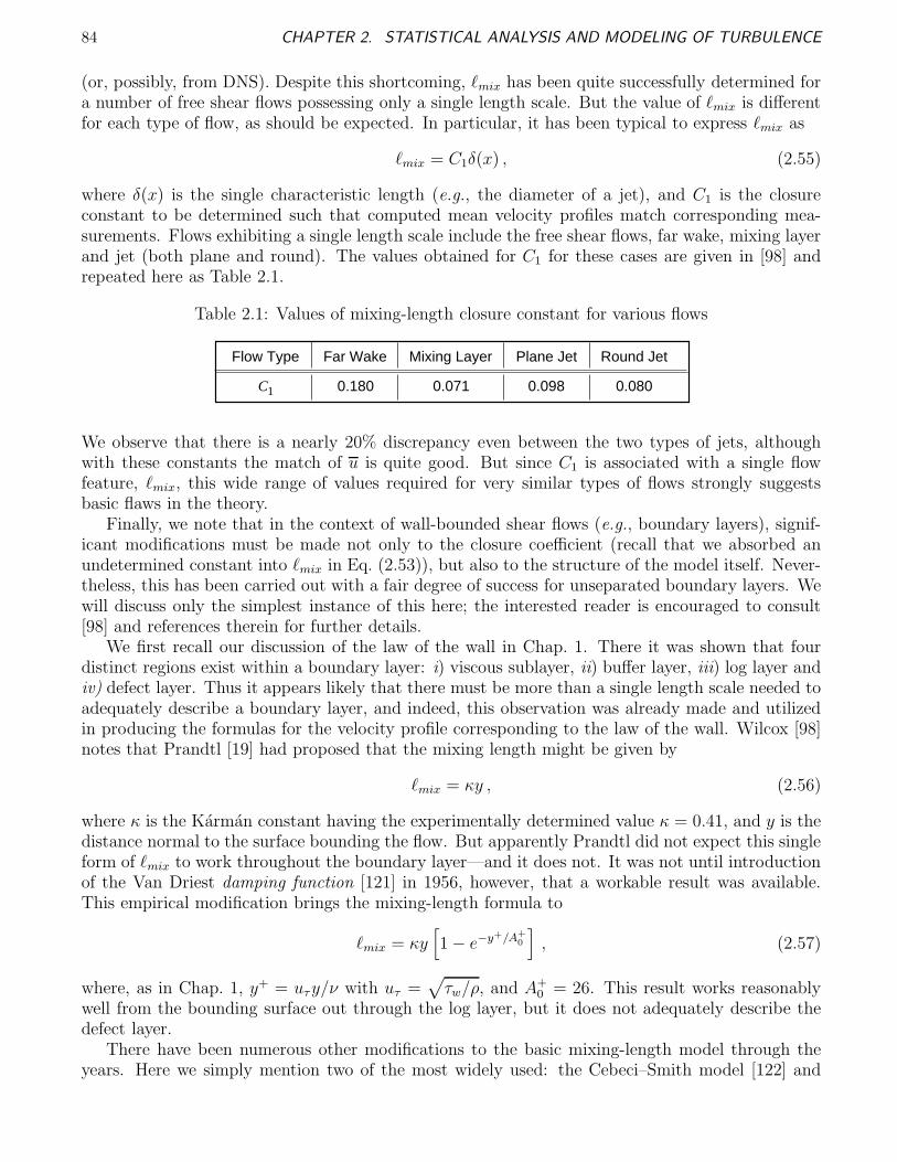
84 CHAPTER 2. STATISTICAL ANALYSIS AND MODELING OF TURBULENCE
(or, possibly, from DNS). Despite this shortcoming, ℓmix has been quite successfully determined fora number of free shear flows possessing only a single length scale. But the value of ℓmix is differentfor each type of flow, as should be expected. In particular, it has been typical to express ℓmix as
ℓmix = C1δ(x) , (2.55)
where δ(x) is the single characteristic length (e.g., the diameter of a jet), and C1 is the closureconstant to be determined such that computed mean velocity profiles match corresponding mea-surements. Flows exhibiting a single length scale include the free shear flows, far wake, mixing layerand jet (both plane and round). The values obtained for C1 for these cases are given in [98] andrepeated here as Table 2.1.
Table 2.1: Values of mixing-length closure constant for various flows
Flow Type Far Wake Mixing Layer Plane Jet Round Jet
C1 0.180 0.071 0.098 0.080
We observe that there is a nearly 20% discrepancy even between the two types of jets, althoughwith these constants the match of u is quite good. But since C1 is associated with a single flowfeature, ℓmix, this wide range of values required for very similar types of flows strongly suggestsbasic flaws in the theory.
Finally, we note that in the context of wall-bounded shear flows (e.g., boundary layers), signif-icant modifications must be made not only to the closure coefficient (recall that we absorbed anundetermined constant into ℓmix in Eq. (2.53)), but also to the structure of the model itself. Never-theless, this has been carried out with a fair degree of success for unseparated boundary layers. Wewill discuss only the simplest instance of this here; the interested reader is encouraged to consult[98] and references therein for further details.
We first recall our discussion of the law of the wall in Chap. 1. There it was shown that fourdistinct regions exist within a boundary layer: i) viscous sublayer, ii) buffer layer, iii) log layer andiv) defect layer. Thus it appears likely that there must be more than a single length scale needed toadequately describe a boundary layer, and indeed, this observation was already made and utilizedin producing the formulas for the velocity profile corresponding to the law of the wall. Wilcox [98]notes that Prandtl [19] had proposed that the mixing length might be given by
ℓmix = κy , (2.56)
where κ is the Karman constant having the experimentally determined value κ = 0.41, and y is thedistance normal to the surface bounding the flow. But apparently Prandtl did not expect this singleform of ℓmix to work throughout the boundary layer—and it does not. It was not until introductionof the Van Driest damping function [121] in 1956, however, that a workable result was available.This empirical modification brings the mixing-length formula to
ℓmix = κy[1 − e−y+/A+
0
], (2.57)
where, as in Chap. 1, y+ = uτy/ν with uτ =√
τw/ρ, and A+0 = 26. This result works reasonably
well from the bounding surface out through the log layer, but it does not adequately describe thedefect layer.
There have been numerous other modifications to the basic mixing-length model through theyears. Here we simply mention two of the most widely used: the Cebeci–Smith model [122] and
2.1. THE REYNOLDS-AVERAGED NAVIER–STOKES EQUATIONS 85
the Baldwin–Lomax model [123]. The former is valid only for 2-D calculations, and while the latteris used in 3-D, it already contains a total of six adjustable closure constants. There are a coupleitems deserving mention here. First, both the Cebeci–Smith and Baldwin–Lomax models providetreatment of the defect layer. But because the precise value of y at which this layer begins is notknown, a priori, it is necessary to construct testable “switching functions” to determine where tobegin using the appropriate formulas for the defect layer. In the case of the Cebeci–Smith model(but not for Baldwin–Lomax) this results in a formula for ℓmix that depends on velocity. In turn,this implies that νT depends on velocity, and it is easy to check that the resulting RANS equationsare no longer Galilean invariant. Proof of this is left as an exercise for the student. The reader willfind further details of these models in [98].
k–ε models. In this section we provide an introductory treatment of the widely-used k–ε models.As might be inferred from the terminology, these are two-equation models. In their basic form theyconsist of a PDE for each of turbulence kinetic energy, k, and turbulence kinetic energy dissipationrate ε. Together, these two quantities provide velocity and length scales needed to directly constructeddy viscosity at each point in a computational domain. In this sense the k–ε models can be viewedas being “closed” because unlike zero- and one-equation models (with the possible exception ofthe Spalart–Allmaras model [124], and other similar ones, for eddy viscosity) these models possesssufficient equations for constructing eddy viscosity with no direct appeal to experimental resultsneeded. We also note that k and ε are not the only variables employed in two-equation models.For example, there are also k–ℓ, k–ω and k–ω2 models, among others. The latter two of these arequite well known, but we leave it to the interested reader to seek more information on these; a goodstarting point is Wilcox [98] and references therein.
We will begin this section with a derivation of a general total kinetic energy equation for incom-pressible flow expressed in its simplest form. We follow this with an outline of the derivation forkinetic energy of the mean flow, again expressed in the simplest manner. Then, following Tennekesand Lumley [7], we present a detailed analysis of the equation for turbulence kinetic energy thatpermits us to analyze the physics represented by each term. But this is not the equation employedin practical calculations, so we next present this with a brief comparison to the theoretical form.We then very briefly treat construction of a PDE for dissipation rate and collect results to obtaina complete k–ε model. We close the section with presentation of some well-known results anddiscussion of the consequences these imply.
To obtain a general energy equation for incompressible flow we simply form the dot product ofthe N.–S. equations with the velocity vector that is their solution. Thus,
U ·(Ut + U ·∇U) = U ·(−∇p + ν∆U ) . (2.58)
A straightforward calculation shows that
∂
∂t
(1
2|U |2
)+ U ·∇
(1
2|U |2
)= −∇·(pU) + ν∆
(1
2|U |2
),
where1
2|U |2 =
1
2(u2 + v2 + w2) ≡ K , (2.59)
the total kinetic energy per unit mass. Thus, the above can be expressed as
Kt + U ·∇K = −∇·(pU) + ν∆K . (2.60)
This equation is a very general result; but at the same time, in the context of incompressible flows,it carries no new information not already found in the N.–S. equations themselves. Nevertheless,
86 CHAPTER 2. STATISTICAL ANALYSIS AND MODELING OF TURBULENCE
we will see that various manipulations of it can lead to useful insights. In this regard we stress thatin the current chapter only the Reynolds decomposition will be studied. But, in fact, essentiallyany decomposition could be used, and as will be apparent as we proceed, details of any associatedanalysis will depend on the form of decomposition employed. Thus, we emphasize that for a LESor Hilbert space decomposition, results we will obtain here would not be valid in detail.
We now introduce the Reynolds decomposition into Eq. (2.59) to obtain
K =1
2
[(u + u′)
2+ (v + v′)
2+ (w + w′)
2]
=1
2
(u2 + v2 + w2
)+
1
2
(u′2 + v′2 + w′2
)+ uu′ + vv′ + ww′
≡ k + k′ + U · U ′ . (2.61)
Finally, we note that the definition of turbulence kinetic energy is
k ≡1
2
(u′2 + v′2 + w′2
)= k′ . (2.62)
We can also construct an energy equation analogous to Eq. (2.60) for the mean flow in exactlythe same way, viz., form the dot product of the mean velocity vector with the RANS equations.This results in
u · ∇k = −∇ · (p u) + ν∆k − u · R(u′, u′) . (2.63)
There are two key observations to make in comparing Eq. (2.63) for the mean flow energy withEq. (2.60) for total energy. First, Eq. (2.63) is a steady-state equation, as it must be, while Eq.(2.60) is time dependent. Second is the appearance of terms involving the Reynolds stress tensor.Particularly the second of these will ultimately play a major role in interpretations given to termsin the equation for turbulence kinetic energy.
We should now observe that we still do not have an equation for what we actually want—theturbulence kinetic energy. Derivation of this is extremely tedious and is essentially always left as“an exercise to the reader.” Here too, we will mainly follow this approach, but we will provide a fewintermediate steps. As noted in [7], the starting point is to time average the total energy equation(2.60), and then subtract the mean flow energy equation (2.63) from this result.
Formal time averaging of (2.60) after substituting the decomposition obtained in Eq. (2.61)yields
U ·∇(k + k′) + U ·∇(U ·U ′) = −∇·(p U) + ν∆(k + k′) ,
and after considerable manipulation this can be expressed as
u·∇(k + k) + ∇·(u′k′
)= −∇(p u) −∇·
(p′u′
)+ ν∆k + ν∆k , (2.64)
where p′ is fluctuating pressure divided by density.We observe that Eq. (2.64) is now steady state, and that it is expressed in terms of both mean
and fluctuating quantities. Subtracting Eq. (2.63) from this leads to an equation for the turbulencekinetic energy:
u·∇k + ∇·(u′k′
)= −∇·
(p′u′
)+ ν∆k + u·R(u′, u′) . (2.65)
But this is not the form found in either [7] or [98], so we need to perform considerable furthermanipulations to arrive at either of these. We will not carry out the details here, but insteadmerely present the results with a brief indication of how they are obtained.
We begin by presenting the results given in each of the two references being used. From Tennekesand Lumley [7] we have
uj∂k
∂xj
= −∂
∂xj
(p′u′
j +1
2u′
iu′iu
′j − 2νu′
is′ij
)− u′
iu′j sij − 2νs′ijs
′ij . (2.66)
2.1. THE REYNOLDS-AVERAGED NAVIER–STOKES EQUATIONS 87
The sij and s′ij represent components of mean and fluctuating strain rate tensors, respectively:
sij =1
2
(∂ui
∂xj
+∂uj
∂xi
), and s′ij =
1
2
(∂u′
i
∂xj
+∂u′
j
∂xi
). (2.67)
Similarly, from Wilcox [98] we obtain
kt + uj∂k
∂xj= −u′
iu′j
∂ui
∂xj− ε +
∂
∂xj
(ν
∂k
∂xj− p′u′
j −1
2u′
iu′iu
′j
), (2.68)
with ε expressed in Cartesian tensor form as
ε = 2νs′ijs′ij . (2.69)
At first glance Eqs. (2.65), (2.66) and (2.68) all appear to be rather different; but with theexception of the time-derivative term (incorrectly) retained in (2.68), these equations are actuallyequivalent. To see this we first note the similarities and then briefly explain the apparent discrep-ancies.
We immediately recognize the term corresponding to advection of turbulence kinetic energyappearing in the left-hand side of all three equations. The only difference between (2.65) and theother two equations is the Cartesian tensor notation employed in the latter two; in particular,we have u ·∇k = uj∂k/∂xj . Similarly, the first term on the right-hand side of (2.65) equals thecorresponding term in (2.66) and the fourth term on the right-hand side of (2.68):
∇·(p′u′
)=
∂
∂xj
(p′u′
j
),
showing the equivalence of these terms. We next observe that the remaining term on the left-handside of Eq. (2.65) is easily shown to be identical to the velocity “triple correlations” appearing inthe right-hand sides of Eqs. (2.66) and (2.68). That is,
∇·(u′k′
)=
1
2
∂
∂xj
u′iu
′iu
′j .
Finally, we easily see that the diffusion terms on the right-hand sides of Eqs. (2.65) and (2.68)exactly match; namely,
ν∆k =∂
∂xj
(ν
∂k
∂xj
),
but there appears to be no corresponding term in Eq. (2.66). At the same time, there seem to be nostrain-rate terms in either of Eqs. (2.65) and (2.68) while there are three such terms in Eq. (2.66).However, using the definition of ε from Eq. (2.69), we see that the last term on the right-hand sideof (2.66) is precisely the ε term of (2.68). Finally, we observe that by making use of the propertiesof the Cartesian tensor notation it can be checked that to within a factor of two, we have
u′iu
′j sij ∼ u′
iu′j
∂ui
∂xj.
Thus, to reconcile the forms of Eqs. (2.66) and (2.68) we must account for the factor of two, andfor the lack of a term in (2.66) corresponding to diffusion of turbulence kinetic energy.
The latter of these is easily explained, and this in turn leads to resolution of the factor of two aswell as all the apparent discrepancies between Eqs. (2.65) and (2.66). In particular, if one beginsderivation of the equation for turbulence kinetic energy with the N.–S. equations expressed in terms
88 CHAPTER 2. STATISTICAL ANALYSIS AND MODELING OF TURBULENCE
of strain rate and ignores the cancellations resulting from the divergence-free condition (as is donein [7]), then one arrives at Eq. (2.66). On the other hand, if this is not done (following the approachwe have taken in the present notes), no explicit strain rate terms appear. This essentially resolvesall differences between Eq. (2.66) and Eq. (2.68).
We still need to provide arguments to show that Eqs. (2.65) and (2.66) are equivalent. The basicone has already been noted, namely, retaining strain rate in lieu of invoking incompressibility toremove most of the terms arising in this representation. But Eq. (2.65) contains a Reynolds stressterm that has not been matched with any terms in either of Eqs. (2.66) and (2.68). It is easilychecked that use of product-rule differentiation permits one to recover the terms u′
iu′j sij of (2.66)
in Eq. (2.65) (recall that R includes a divergence operator), but additional terms also arise. Similarproduct-rule differentiations in the strain rate terms (along with judicious combinations of thesewith terms from the Reynolds stress tensor) lead to the remaining terms appearing in (2.66). Asindicated in [7], these are very tedious calculations, and they will not be repeated here.
The point of this rather lengthy development is the following. The derivation we have providedfor Eq. (2.65) is fairly easy and straightforward and corresponds to a purely math-oriented approach.The form corresponding to Eq. (2.66) leads to a number of significant physical insights as we willbriefly discuss below, and Eq. (2.68) is directly related to the turbulence energy equation actuallyused in RANS models. Thus, each form has an important application, and demonstration of theirequivalence is important.
The physical interpretation of terms in Eq. (2.66), as presented in [7], can be summarized asfollows. As already mentioned, the term on the left-hand side is simply advection of turbulencekinetic energy, and the first term on the right-hand side represents pressure work due only toturbulence. The second term on the right-hand side corresponds to transport of turbulence kineticenergy by turbulent fluctuations, which is more clearly seen in the equivalent term appearing on theleft-hand side of Eq. (2.65). Tennekes and Lumley [7] describe the next term on the right-hand side,2νu′
is′ij, as “transport by viscous stresses,” but they do not make clear what is being transported.
Indeed, Eq. (2.66) is a transport equation for turbulence kinetic energy; but if the term in questionis accomplishing transport by viscous stresses, then it is clear that it is not kinetic energy that isbeing transported, but rather simply the turbulent fluctuations. In fact, from our earlier discussionsit is evident that this term is actually associated with the diffusive transport of turbulence kineticenergy which is the same as transport of viscous stresses, but is an intuitively clearer concept.
Tennekes and Lumley [7] associate the final two terms on the right-hand side of Eq. (2.66) with“two kinds of deformation work.” They term the first of these “turbulence production,” and usethe notation
P ≡ −u′iu
′j sij (2.70)
to identify it. We see from this that what is actually represented is amplification of the Reynoldsstress tensor components by the mean strain rate. We have already argued that this is equivalentto the first term on the right-hand side of Eq. (2.68), and that it arises from rearrangement of termsinvolving the Reynolds stress tensor as appears on the right-hand side of (2.65). We remark thatif true “scale separation” occurs, as is usually supposed in the context of model construction, wemust question whether the mean strain rate would actually be capable of interaction with Reynoldsstress components.
The final term on the right-hand side of Eq. (2.66) is described in [7] as the “rate at whichfluctuating viscous stresses (νs′ij) perform deformation work against the fluctuating strain rate
(s′ij).” But we have already seen that the term νs′ijs′ij is (up to a constant factor) simply the
dissipation rate of turbulence kinetic energy given in Eq. (2.69). A physical interpretation based onthe latter description seems far more intuitive, especially with regard to the purported consequences.
At this point it is worthwhile to observe, as noted in [7], that ε ≃ P often holds, at least
2.1. THE REYNOLDS-AVERAGED NAVIER–STOKES EQUATIONS 89
in an order-of-magnitude sense; that is, dissipation of turbulence kinetic energy by viscosity isapproximately equal to its production via strain rate amplification of Reynolds stress. Recall thatwe earlier, in Def. 1.70, termed this type of situation “equilibrium turbulence.” This correspondsto
−u′iu
′j sij = 2νs′ijs
′ij . (2.71)
We immediately note that the right-hand side of this expression is nonnegative, which impliesthat velocity correlations and corresponding mean strain rates would be expected to usually haveopposite signs. On the other hand, we must be careful to recognize that Eq. (2.71) does not oftenhold exactly, and as also observed in [7], it will seldom be satisfied for shear flows. If we recallthe Galerkin form of the N.–S. equations presented in Chap. 1, we see that “production” actuallyarises simply from the nonlinear terms, and dissipation is a result of only the diffusive terms.On small scales (high wavenumbers) it is indeed a “balance”—not necessarily equality—of thesethat produces the strange attractor of the dynamical system. At the same time, if equality holdsover essentially all scales (implied by mathematics of the Reynolds decomposition) as required inequilibrium turbulence, the Galerkin form of the equations of motion collapses to triviality. This allreflects the difficulties that can arise when one attempts to associate physics with quantities thatare merely statistical. Nevertheless, the authors of [7] proceed to derive the estimate
s′ijs′ij ≫ sij sij (2.72)
using Eq. (2.71). Indeed, the magnitude of the difference between these two parts of the strain ratetensor is of the order of the integral scale Reynolds number, Reℓ. Despite the rather unrealisticassumptions made in [7] in the course of obtaining the inequality (2.72) (equilibrium turbulence withsingle length and velocity scales), it is an expected result from the standpoint of our understanding ofthe mathematical nature of solutions to the N.–S. equations. We recall that a feature of turbulentsolutions is their intrinsic nonsmoothness, particularly in their high-wavenumber/high-frequencycomponents; that is, spatial derivatives on small scales can be expected to be much larger thanthose on larger scales. Since strain rates are simply combinations of spatial derivatives, inequality(2.72) is completely consistent with this.
We are now prepared to return to Eq. (2.68), the form of the turbulence kinetic energy equationemployed for computations, and indicate how it is converted to the form usually taken in k–εmodels. We begin by observing that there are three terms that must be modeled, a remainingone that will be computed from a PDE, which itself requires very significant modeling, and thenconstruction of eddy viscosity from the results of all this. These terms correspond to production,pressure work, velocity triple correlation and dissipation. Following Wilcox [98] we employ theBoussinesq hypothesis in the form
−u′iu
′j = 2νT sij −
2
3kδij (2.73)
to model the Reynolds stress factor in the production term. The second term in this expressionaccounts for the fact that the trace of the strain rate tensor is zero for an incompressible flow, andis thus necessary to provide consistency with the definition of turbulence kinetic energy k from Eq.(2.62) when i = j. We remark, however, that this results in employing normal viscous stress termsin the absence of eddy viscosity which is logically inconsistent with the Boussinesq hypothesis.Despite this, it is useful to recognize that Eq. (2.73) provides a means to calculate each term of theReynolds stress tensor once a calculation of the mean velocity has been completed. Thus, second-moment information can be retrieved even though we have not directly calculated it as we would ina second-moment closure approach. In principle, this is true for any model employing a Boussinesqhypothesis; in particular, once the mean velocity field has been obtained, if νT is available, we candirectly compute the u′
iu′js.

90 CHAPTER 2. STATISTICAL ANALYSIS AND MODELING OF TURBULENCE
We next consider approximation of the pressure work term p′u′j appearing in the right-hand
side of Eq. (2.68). To accomplish this we first observe that a slight modification of the Boussinesqhypothesis leads to an approximation of scalar turbulent fluxes analogous to the Reynolds stresscomponent fluctuations. For example, suppose we decompose temperature as T = θ + θ′. Thenthe Reynolds-averaged thermal energy equation will contain terms of the form u′
jθ′ known as scalar
fluxes, and these are approximated as (νT /σT )∂θ/∂xj where σT is the turbulent Prandtl number.So one might suppose that we could represent the pressure work term (usually called pressurediffusion in the modeling literature) as p′u′
j = νT ∂p/∂xj . But this does not work. Indeed, it is clearthat pressure does not satisfy a transport equation, so the notion of pressure diffusion is completelyfallacious. Much effort has been devoted to modeling this term, and rather complicated results havebeen obtained and used in the context of second-moment closures (see [98]). There is little physicalor mathematical justification for any of these, so we will not provide any further descriptions.
Within the confines of k–ε models a simpler approach is usually taken. This begins by alsorecognizing that we have little in the way of sound theory for modeling the velocity triple correlation.So we (arbitrarily) combine this with the pressure diffusion term and model these together as“diffusion of kinetic energy:”
−p′u′j −
1
2u′
iu′iu
′j =
νT
σk
∂k
∂xj. (2.74)
Here, σk is an additional closure constant. We emphasize that there is no physical justification foruse of Eq. (2.74). It is merely a convenience that permits us to express Eq. (2.68) as
∂k
∂t+ uj
∂k
∂xj= −u′
iu′j
∂ui
∂xj− ε +
∂
∂xj
[(ν + νT /σk)
∂k
∂xj
]. (2.75)
It is worthwhile to point out the types of terms appearing in this equation because it is commonpractice in RANS modeling to presume all turbulence quantities, physical or otherwise, satisfytransport equations of this basic form. Thus, we observe that in addition to the time-dependentterm on the left-hand side there is also advection (macroscopic transport) of kinetic energy. On theright-hand side we find production, dissipation and diffusion of kinetic energy. This is almost alwaysthe point of departure for construction of essentially all such models. The fact that there is no apriori reason to expect that many such quantities (e.g., eddy viscosity, as in the Spalart–Allmarasmodels) should satisfy a transport equation is never considered.
We have yet to construct a model for ε. We begin this by recalling the definition from Eqs. (2.67)and (2.69). Clearly, a model is needed since we do not know u′
i, and we therefore cannot computethe required derivatives. We also observe that when we present the equation for second-momentclosure in the next section we will see that within this context dissipation of turbulence kineticenergy is a second-rank tensor—a matrix:
εij = 2ν∂u′
i
∂xk
∂u′j
∂xk
.
So the first approximation we make here in our effort to model dissipation as it appears in (2.75)is the usual one; that is, dissipation is locally isotropic, meaning that small-scale (high wavenum-ber) behavior is independent of direction and satisfies required rotation and reflection propertiesdiscussed earlier. Then we express the above as
εij =2
3εδij ,
with
ε ≡ ν∂u′
i
∂xk
∂u′i
∂xk
. (2.76)

2.1. THE REYNOLDS-AVERAGED NAVIER–STOKES EQUATIONS 91
Effects of this, and modifications, have been widely studied (see [98] and references therein), andwe will not dwell on this in these lectures. We mention, however, that in the context of a Reynoldsdecomposition it is much more difficult to justify invocation of a local isotropy hypothesis thanis the case for a LES decomposition for the simple reason that the u′
i represent far more thanhigh-wavenumber behavior, in general, in the present case.
Even within the confines of local isotropy, the equation for ε is difficult to derive, and it introducesa total of six new higher-order correlations that must be modeled. These are all statistical, and asnoted by Wilcox [98], the result is not a model of physics but rather a model of the original PDE(s)associated with the tensor components εij. Nevertheless, it is widely used, and we present it here:
∂ε
∂t+ uj
∂ε
∂xj
= −Cε1ε
ku′
iu′j
∂ui
∂xj
− Cε2ε2
k+
∂
∂xj
[(ν + νT /σε)
∂ε
∂xj
].
This equation contains three new closure constants, Cε1, Cε2 and σε. But assuming values of thesecan be found, it can be seen that we now have a complete system of equations. In particular, weobserve that the required length and velocity scales needed for construction of νT now are availableat each point of a computational grid. To see this, we note that k ∼ (L/T)2, and ε ∼ L2/T3. Thus,we immediately obtain a velocity scale from k1/2, as is obvious; moreover, it is clear that k/ε ∼ T.It then follows that k3/2/ε ∼ L, and since νT ∼ L2/T, we obtain
νT = Cνk2
ε,
where Cν is a constant needed to account for the fact that this has been derived entirely viadimensional analysis. It is important to recognize that with νT given in this form the diffusionterms of the kinetic energy and dissipation equations become highly nonlinear, and while fairlyelaborate numerical techniques probably should be employed to handle this, in practice this isseldom done.
We now collect the complete set of equations comprising the “standard” k–ε RANS model.These consist of the mean flow continuity and momentum equations, with the latter containingthe eddy viscosity, the equations for turbulence kinetic energy and its dissipation rate, and thosecorresponding to the Boussinesq hypothesis and eddy viscosity in this context. Thus, we have thefollowing:
∇·u = 0 , (2.77a)
ut + u·∇u = −∇p + ∇·[(ν + νT )∇u] , (2.77b)
kt + u·∇k = P − ε + ∇·[(ν + νT /σk)∇k] , (2.77c)
εt + u·∇ε = Cε1ε
kP − Cε2
ε2
k+ ∇·[(ν + νT /σε)∇ε] , (2.77d)
with production P given by
P = −u′iu
′j
∂ui
∂xj, (2.78a)
−u′iu
′j = 2νT sij −
2
3kδij , (2.78b)
and
νT = Cνk2
ε. (2.79)
The closure constants corresponding to the so-called standard k–ε model are:
Cν = 0.09 , Cε1 = 1.44 , Cε2 = 1.92 , σk = 1.0 , σε = 1.3 . (2.80)
92 CHAPTER 2. STATISTICAL ANALYSIS AND MODELING OF TURBULENCE
It is clear that this provides a completely closed system for computing u, p, k and ε, and from(2.78b) all components of the Reynolds stress tensor.
Several remarks are in order regarding Eqs. (2.77)–(2.80). The first, and possibly most impor-tant, is that they cannot be integrated all the way to a solid boundary. Instead, the law of the wallmust be employed to provide velocity “boundary conditions” away from solid boundaries. Numer-ous physical arguments have been proposed to explain this (e.g., approximations made to obtainequations for k and ε are not strictly valid in the viscous sublayer), but the simplest follows directlyfrom the mathematics of the energy dissipation equation Eq. (2.77d). It is clear from the definitionof ε, Eq. (2.76), that ε will not generally go to zero approaching a solid boundary. At the same timewe see from Eq. (2.62) that k → 0 as a solid boundary is approached. Now the term involving P inEq. (2.77d) approaches zero near solid surfaces, but the term containing ε2/k is singular. Clearly,if we can assign Dirichlet conditions for ε on solid boundaries this formally removes the singularitysince in this case the dissipation rate equation will not be solved on the boundary. But despite this,as gridding is refined, the ε2/k term can become large at the first few grid points near the boundary,and thus difficult to handle from a computational aspect. In particular, this is often associated with“stiffness” of the numerical problem.
The simplest way to avoid this difficulty is to employ the law of the wall to permit assigningvelocity (and all other) conditions at a distance from the wall corresponding to somewhere in the loglayer. One must be somewhat careful with this, however. It is well known that turbulence kineticenergy attains its maximum fairly close to the wall (but somewhere in the log layer) for wall-boundedshear flows. Thus, if one is to have any hope of predicting this correctly it is necessary to evaluatethe log law fairly close to the wall to find the required velocity boundary condition. We also notethat the specific difficulty we have analyzed here is not present if we employ Neumann conditions onsolid walls for the dissipation rate equation. In some respects, this might be preferable in any casesince there is actually no way to accurately assign Dirichlet conditions for dissipation rate. Another,somewhat more complicated, approach is to employ the so-called “low-Re” k–ε formalisms in thevicinity of solid boundaries. Treatment of these can be found in [98] and references therein.
The second observation is that the equations for kinetic energy and dissipation rate are stronglycoupled with each other, but only weakly so with the momentum equations. This suggests thatsignificant difficulties can arise in solution procedures for the k and ε equations which are not presentfor the momentum equations alone. Moreover, little mathematical analysis has been applied tothese equations beyond the rather naıve treatment provided by Mohammadi and Pironneau [125].In particular, these equations exhibit, in addition to their stronger coupling, forms of nonlinearitynot generally encountered in transport equations raising numerous questions regarding existenceand uniqueness of their solutions, and their regularity. Even in the absence of these questions thereclearly is significant extra computer arithmetic because there are two additional nonlinear PDEs tobe solved.
In general, assignment of boundary conditions, for k and ε is difficult. We have already mentionedthe problems with ε on solid walls. But at inflows and outflows values are not known for eitherk or ε. For outflows it is common practice (although not necessarily accurate) to assume fully-developed flow and employ homogeneous Neumann conditions for both of these. But at inflows thisis not valid, and it is difficult to obtain accurate conditions, especially for ε. Indeed, both k andε are statistical, rather than physical, so it is not easy to deduce their values simply from physicalconsiderations alone.
Finally, we note that the definition of νT in terms of k and ε renders the system of equations nolonger Galilean invariant. (We leave demonstration of this as an exercise for the reader; consultationof [99] may be helpful.) As we have emphasized earlier, Galilean invariabnce is a crucial physicalproperty of solutions to the N.–S. equations, and its lose during construction of any turbulencemodel must cast strong doubts on validity of such a model.
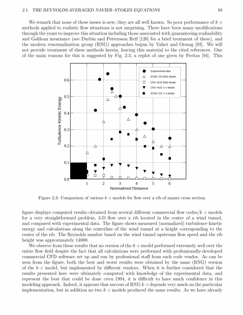
2.1. THE REYNOLDS-AVERAGED NAVIER–STOKES EQUATIONS 93
We remark that none of these issues is new; they are all well known. So poor performance of k–εmethods applied to realistic flow situations is not surprising. There have been many modificationsthrough the years to improve this situation including those associated with guaranteeing realizabilityand Galilean invariance (see Durbin and Pettersson Reif [126] for a brief treatment of these), andthe modern renormalization group (RNG) approaches begun by Yahot and Orszag [93]. We willnot provide treatment of these methods herein, leaving this material to the cited references. Oneof the main reasons for this is suggested by Fig. 2.3, a replot of one given by Freitas [94]. This
0.1
0.2
0.3
0.4
0.5
0.6
Normalized Distance
0.0651 2 3 4
Tur
bule
nce
Kin
etic
Ene
rgy
k
CFD−ACE RNG Model
STAR−CD RNG Model
Experimental data
STAR−CD Model−εk
−εCFD−ACE Model
Figure 2.3: Comparison of various k–ε models for flow over a rib of square cross section.
figure displays computed results obtained from several different commercial flow codes/k–ε modelsfor a very straightforward problem, 3-D flow over a rib located in the center of a wind tunnel,and compared with experimental data. The figure shows measured (normalized) turbulence kineticenergy and calculations along the centerline of the wind tunnel at a height corresponding to thecenter of the rib. The Reynolds number based on the wind tunnel upstream flow speed and the ribheight was approximately 14000.
We observe from these results that no version of the k–ε model performed extremely well over theentire flow field despite the fact that all calculations were performed with professionally-developedcommercial CFD software set up and run by professional staff from each code vendor. As can beseen from the figure, both the best and worst results were obtained by the same (RNG) versionof the k–ε model, but implemented by different vendors. When it is further considered that theresults presented here were ultimately computed with knowledge of the experimental data, andrepresent the best that could be done circa 1994, it is difficult to have much confidence in thismodeling approach. Indeed, it appears that success of RNG k–ε depends very much on the particularimplementation, but in addition no two k–ε models produced the same results. As we have already
94 CHAPTER 2. STATISTICAL ANALYSIS AND MODELING OF TURBULENCE
emphasized, this poor performance is not unexpected; the Boussinseq hypothesis lacks any rigorousphysical justification, and as a consequence, for anything but the simplest flows it cannot be expectedto provide adequate accuracy, almost independent of the implementation. But as we have alreadyobserved, there are further (unjustified) approximations made in the derivations of both the k andε equations, and beyond this the fundamental flaws inherent in all Reynolds-averaged approaches.
Second-moment closure (SMC) models. The poor results produced by k–ε models have longsuggested attempting use of models “containing more physics.” Recall that the Reynolds stressesarising in the RANS formulation are modeled entirely in terms of the Boussinesq hypothesis ink–ε models, and as we have already seen, reasons can be cited for probable failure of this for mostnontrivial physical flows. Launder et al. [63] first proposed use of second-moment closure (alsoknown as Reynolds stress models, RSMs) in 1975 shortly after introduction of the modern k–εmodels. Such methods provide PDEs for each component of the Reynolds stress tensor rather thandepending on the Boussinesq hypothesis. But as we will show, these equations contain so manyunclosed terms which themselves must be modeled, often in nearly arbitrary ways (including analogsof the Boussinesq hypothesis), that it is rather doubtful much has been gained. Moreover, in 3-Dcalculations typically nine PDEs must be solved, compared with four for the N.–S. equations alone,and six for k–ε models. Thus, the computational expense is extremely high, approaching that ofDNS for low-Reynolds number calculations. On the other hand, the total arithmetic required bySMCs is not strongly dependent on Re, so at least in principle these might be used effectivelyfor high-Re flow calculations not currently accessible by DNS. Indeed, commercial CFD codes arebeginning to contain SMC options.
Herein we will provide a simple derivation of the equations corresponding to typical SMCs, forthe most part following Wilcox [98] but employing somewhat different notation more consistentwith that used throughout these lectures.
The RANS equations used in conjunction with SMC models are the same as originally derived,but they are typically expressed in a form containing the temporal derivative operators. Thus, inthe context of Cartesian tensor notation these are
∂ui
∂t+ uj
∂ui
∂xj= −
∂p
∂xi+ ν
∂2ui
∂xj∂xj−
∂(u′
iu′j
)
∂xj, i = 1, 2, 3 , (2.81)
along with the divergence-free condition ∂ui/∂xi = 0.
Now let NS(Ui) denote the Navier–Stokes operator for the ith component of velocity; i.e., wehave
NS(Ui) ≡
(∂
∂t+ U ·∇ − ν∆
)Ui +
∂P
∂xi
= 0 , i = 1, 2, 3 . (2.82)
Then to derive the equation for the Reynolds stress component u′iu
′j we form
u′i NS(Uj) + u′
j NS(Ui) = 0 , i, j = 1, 2, 3 , i 6= j . (2.83)
We now carry out the indicated operations in a term-by-term fashion.
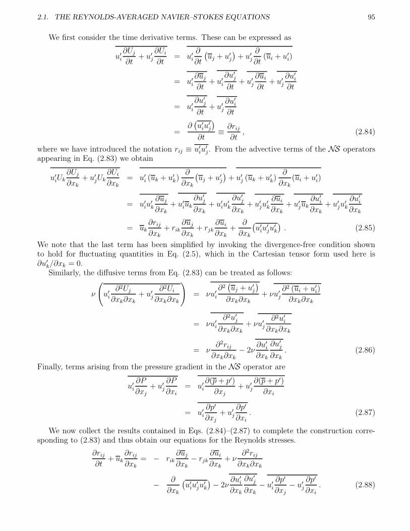
2.1. THE REYNOLDS-AVERAGED NAVIER–STOKES EQUATIONS 95
We first consider the time derivative terms. These can be expressed as
u′i
∂Uj
∂t+ u′
j
∂Ui
∂t= u′
i
∂
∂t
(uj + u′
j
)+ u′
j
∂
∂t(ui + u′
i)
= u′i
∂uj
∂t+ u′
i
∂u′j
∂t+ u′
j
∂ui
∂t+ u′
j
∂u′i
∂t
= u′i
∂u′j
∂t+ u′
j
∂u′i
∂t
=∂(u′
iu′j
)
∂t≡
∂rij
∂t, (2.84)
where we have introduced the notation rij ≡ u′iu
′j. From the advective terms of the NS operators
appearing in Eq. (2.83) we obtain
u′iUk
∂Uj
∂xk
+ u′jUk
∂Ui
∂xk
= u′i (uk + u′
k)∂
∂xk
(uj + u′
j
)+ u′
j (uk + u′k)
∂
∂xk
(ui + u′i)
= u′iu
′k
∂uj
∂xk
+ u′iuk
∂u′j
∂xk
+ u′iu
′k
∂u′j
∂xk
+ u′ju
′k
∂ui
∂xk
+ u′juk
∂u′i
∂xk
+ u′ju
′k
∂u′i
∂xk
= uk∂rij
∂xk+ rik
∂uj
∂xk+ rjk
∂ui
∂xk+
∂
∂xk
(u′
iu′ju
′k
). (2.85)
We note that the last term has been simplified by invoking the divergence-free condition shownto hold for fluctuating quantities in Eq. (2.5), which in the Cartesian tensor form used here is∂u′
k/∂xk = 0.Similarly, the diffusive terms from Eq. (2.83) can be treated as follows:
ν
(u′
i
∂2Uj
∂xk∂xk+ u′
j
∂2Ui
∂xk∂xk
)= νu′
i
∂2(uj + u′
j
)
∂xk∂xk+ νu′
j
∂2 (ui + u′i)
∂xk∂xk
= νu′i
∂2u′j
∂xk∂xk+ νu′
j
∂2u′i
∂xk∂xk
= ν∂2rij
∂xk∂xk
− 2ν∂u′
i
∂xk
∂u′j
∂xk
. (2.86)
Finally, terms arising from the pressure gradient in the NS operator are
u′i
∂P
∂xj
+ u′j
∂P
∂xi
= u′i
∂(p + p′)
∂xj
+ u′j
∂(p + p′)
∂xi
= u′i
∂p′
∂xj+ u′
j
∂p′
∂xi. (2.87)
We now collect the results contained in Eqs. (2.84)–(2.87) to complete the construction corre-sponding to (2.83) and thus obtain our equations for the Reynolds stresses.
∂rij
∂t+ uk
∂rij
∂xk= − rik
∂uj
∂xk− rjk
∂ui
∂xk+ ν
∂2rij
∂xk∂xk
−∂
∂xk
(u′
iu′ju
′k
)− 2ν
∂u′i
∂xk
∂u′j
∂xk
− u′i
∂p′
∂xj
− u′j
∂p′
∂xi
. (2.88)
96 CHAPTER 2. STATISTICAL ANALYSIS AND MODELING OF TURBULENCE
We observe that for each i, j = 1, 2, 3 the first line of this tensor equation could be directlysolved for the rijs. This comprises a system of six independent equations coupled with Eqs. (2.81)for the mean flow quantities. All of the terms in the second line, however, must be modeled in orderto accomplish this and thus close the SMC formulation.
Following [98] we first note the extent of this task. The first term in the second line of Eq. (2.88)is divergence of the velocity triple correlations u′
iu′ju
′k, which when expanded taking into account
the summation convention and the i-j, etc. symmetries results in a total of 10 independent terms.There are six further terms from expansion of the second term on line 2 of (2.88), which we recognizeas the dissipation rate tensor also defined earlier in connection with the k–ε method. Finally, thereare six more terms arising in the pressure-velocity correlations, the last terms on the second lineof (2.88). Thus, there are now a total of 22 additional unknowns. (The reader will recall thatthere were only eight such terms appearing in the k–ε formulation once the Boussinesq hypothesiswas invoked.) These are all statistical quantities with little verifiable physical relevance althoughmuch effort has been devoted to attempts to ascribe such relevance to them. (See [98] for a slightlydifferent arrangement of (2.88) which is cast in terms of such physical interpretations.) So, despitethe fact that SMCs are claimed to “contain more physics” than do k–ε models, in reality if thiswere actually true to begin with (which requires contrived interpretations to argue), any benefitsof this additional physics are likely to be lost in the modeling of these terms. In the end, what isactually accomplished is not a model containing more physics but rather one containing far moreclosure “constants” that can be adjusted at will in efforts to match observed flow field behaviors.But there is no significantly improved predictability.
Summary of RANS Modeling
We summarize the preceding discussions of RANS methods as follows. After introducing commonly-used terminology we provided a fairly detailed treatment of the Boussinesq hypothesis, emphasizingits fundamental shortcomings. The main ones of these are its lack of physical basis and the needto compute eddy viscosity (which is actually a tensor) in order to use it. We then discussed inconsiderable detail two of the main classes of RANS methods still in wide use, namely Prandtl’smixing-length theory and the k–ε models. The first of these is an algebraic model while the secondis of the two-equation type. Both of these explicitly employ the Boussinesq hypothesis to convertfluctuating (nonlinear) advective terms of the N.–S. equations to mean (linear) diffusive ones. Inaddition, the k–ε methods require completely unsubstantiated modeling of various other statisticalterms to arrive at the final forms used in computational procedures. We then presented specificresults from the extant literature that demonstrate the inadequacies of the k–ε models when appliedto nontrivial flows.
Following this we briefly described second-moment closures which were introduced specifically toinclude “more physics” in turbulence models. These approaches utilize PDEs to directly computeReynolds stress tensor components rather than relying in the Boussinesq-hypothesis model. Unfor-tunately, the process of obtaining these equations leads to a total of 22 unclosed statistical termsthat must be modeled. Most of these are sufficiently removed from actual physics that there is littleguidance in constructing their models, and the end result is that SMCs are “models of differentialequations” rather than models containing more physics. Experience with these to date has beenonly slightly better than that with k–ε models, but with an extremely increased arithmetic penalty.As a consequence, they are not widely used.
2.2. THE KOLMOGOROV THEORY OF TURBULENCE 97
2.2 The Kolmogorov Theory of Turbulence
The Kolmogorov theory of turbulence published in a series of three brief papers [26] in 1941 is one ofthe most quoted, and yet least well understood of turbulence theories. It is not well understood,atleast in part, because the original papers are difficult to read: the assumptions made are not clearlystated, and the purportedly proven results do not clearly follow from the assumptions—becausethey are highly nontrivial. On the other hand, these results have withstood the “test of time,”and in general should be viewed as correct within the confines of the assumptions made to obtainthem. The monograph by Frisch [80] and references therein provide a very good but still not easilycomprehended modern treatment and interpretation of this seminal work. In the present lectureswe will only briefly summarize Frisch’s treatment by stating main hypotheses and results, but notattempting the detailed proofs provided in [80].
We will begin by stating Kolmogorov’s “universality assumptions,” and then introduce threerelated hypotheses employed by Frisch [80] to prove the celebrated 4/5 law. We then present thethree main results provided by Kolmogorov in 1941 (known as the K41 theory), and discuss someof the consequences of these.
2.2.1 Kolmogorov’s “universality” assumptions
Before presenting specific statements of these assumptions it is worthwhile to briefly consider theoverall setting in which they were made. In particular, we should recall the general nature ofsolutions to the Navier–Stokes equations, viz., that they possess certain symmetries (discussed inChaps. 1 and 2 of [80] and in Sec. 1.4.3 of these notes) at very low Reynolds number which aresuccessively broken as Re is increased, and which are ultimately recovered in a statistical sense asRe becomes very large and the flow becomes turbulent. Within this framework Kolmogorov’s firstuniversality assumption (also called his “first similarity hypothesis”) is the following:
Kolmogorov’s first universality assumption. At very high, but not infinite, Reynolds number,all of the small-scale statistical properties are uniquely and universally determined by the lengthscale ℓ, the mean dissipation rate (per unit mass) ε and the viscosity ν.
Similarly, the second universality assumption is as follows:
Kolmogorov’s second universality assumption. In the limit of infinite Reynolds number, allsmall-scale statistical properties are uniquely and universally determined by the length scale ℓ andthe mean dissipation rate ε.
It is worthwhile at this point, before proceeding further, to clarify terminology and notation.First, it is important to note that both of these statements concern “small-scale” statistical prop-erties. Thus, we need first to indicate precisely what is meant by small scale. Indeed, this is notthe same as the fluctuating quantities in a Reynolds decomposition (although classical turbulencetheorists often equate these). In the first place, we should recall that the lowest moments of thefluctuating quantities in a Reynolds decomposition are null; for example, u′ = 0. In the presentcase we should associate small-scale quantities with the high-pass filtered part of a N.–S. solution,i.e., the high-wavenumber/high-frequency components. Thus, in the context of our Hilbert-spacedecomposition discussed earlier, the small-scale part would be, e.g.,
u′(x, t) =∑
|k|>kc
ak(t)ϕk(x) . (2.89)
Clearly, in this case we would generally expect u′ 6= 0. A slightly different, but related (essentiallyequivalent) interpretation of small scale is to associate this with length scales that are very muchsmaller than the integral scale.
98 CHAPTER 2. STATISTICAL ANALYSIS AND MODELING OF TURBULENCE
We can now compare details of Kolmogorov’s two similarity hypotheses. The first of theseconcerns finite-Re behavior and as such implies that statistics will be uniquely (and universally) setby length and dissipation scales, and viscosity. The second hypothesis, on the other hand, concernsthe Re → ∞ limit. In this case we expect ν → 0, so the universal statistical behaviors should nolonger depend on ν. We remark that it is this hypothesized universality that causes most problems(and criticisms) regarding these assumptions. It should also be mentioned that the flow propertieshomogeneity and (local) isotropy are generally regarded as being essential to applicability of theKolmogorov theory, but we see neither of these explicitly required in the similarity hypotheses. Wewill see below, however, that these will be needed in order to prove the 4/5 law.
2.2.2 Hypotheses employed by Frisch [80]
Treatment of the Kolmogorov theory provided by Frisch is the outgrowth of many careful andthorough examinations and analyses by a number of researchers during the 1980s and early 1990s,and it has culminated in a much more easily understood representation of this theory. We willprovide an abbreviated, and slightly reorganized, version of this in the present lectures. The startingpoint is the set of three hypotheses put forth by Frisch in [80]. These can be stated as follows.
Hypothesis 1. In the Re → ∞ limit, all possible symmetries of the N.–S. equations, usually brokenby the (physical) mechanisms producing turbulence, are restored in a statistical sense at small scalesand away from boundaries.
Hypothesis 2. Under the same assumptions as above, turbulent flow is self similar at small scales;i.e., it possesses a unique scaling exponent h such that
δu(x, λℓ) = λhδu(x, ℓ) , ∀ λ ∈ R+ , x ∈ R3 , (2.90)
with increments ℓ and λℓ small compared with the integral scale.
Hypothesis 3. Again, under the same assumptions as in Hypothesis 1, turbulent flow has a finite,nonvanishing mean rate of dissipation per unit mass, ε.
It is important to consider some of the details and implications of these hypotheses and, further,to compare them with Kolmogorov’s two original universality assumptions. We should first note,again, that small scales are associated with length scales very much smaller than the integral scale.As explained in [80], we can interpret small-scale homogeneity, for example (the requirement forwhich is not explicitly stated), in the context of velocity increments
δu(x, ℓ) ≡ u(x + ℓ) − u(x) , (2.91)
and in particular require that statistics of these increments be invariant under arbitrary translationsr for stationary flows. That is, e.g.,
〈δu(x + r, ℓ)〉 = 〈δu(x, ℓ)〉 ,
where 〈 · 〉 denotes any generic averaging procedure, as described in Chap. 1. A similar interpretationapplies to isotropy of velocity increments in which invariance must hold under arbitrary rotationsof ℓ and δu.
We now provide a few clarifying remarks associated with each of these hypotheses. First, taken asa whole, they are used to obtain consequences of the 2/3 law and proof of the 4/5 law. Also, we notethat they are not identical with the Kolmogorov universality assumptions. In this regard, we observe(as does Frisch, himself) that Frisch does not employ the first of the Kolmogorov assumptions; inparticular, all of the hypotheses used in [80] involve the Re → ∞ limit. Second, all three of Frisch’s
2.2. THE KOLMOGOROV THEORY OF TURBULENCE 99
hypotheses require the assumption of recovery of N.–S. symmetries in the statistical sense, whilethe Kolmogorov assumptions do not explicitly state this. It is, however, needed in the proofs ofthe Kolmogorov results, but it is not clear that Kolmogorov actually intended this simply becauseexperimental evidence of this property was not yet particularly strong at the time of his K41analyses. The final aspect of Frisch’s first hypothesis is the requirement of being “away fromboundaries.” Again, this did not explicitly appear in the Kolmogorov assumptions, and it is thefirst hint that homogeneity and or isotropy will be invoked—neither of these can be expected tohold in the vicinity of (solid) boundaries.
It is important to consider the details of Frisch’s Hypothesis 2. It proposes self similarity onsmall scales and expresses this in terms of a typical power law representation. We earlier providedan heuristic description of self similarity in Def. 1.45; here, Eq. (2.90) establishes a more concretecharacterization in terms of velocity increments. It is worth noting that this is a vector expression;but λ and h are scalars, and this is hypothesized to hold for all spatial increments ℓ and positivemultipliers λ provided these are small compared with the integral scale. We remark that this seemsbasically equivalent to small-scale homogeneity and isotropy assumptions, the latter due to thevector nature of Eq. (2.90). We also mention that this equation expresses a “pure math” versionof homogeneity of velocity increments; viz., it is precisely a statement that these are “homogeneousof degree h,” a concept often encountered in analysis of differential equations—e.g., dynamicalsystems. At the same time, the power law representation is typical of characterizations associatedwith fractal attractors of differential (and discrete) dynamical systems, and often phase portraitsof their trajectories appear the same on all scales (see, for example, Alligood et al. [85]).
Finally, Hypothesis 3 coincides with experimental observations, and it also embodies importantmathematical consequences. To understand the nature of these we again recall the definition ofdissipation rate, given originally in Eq. (1.53):
ε = 2ν‖S‖2 ,
where S is the strain rate tensor whose elements are of the form
Sij =1
2
(∂ui
∂xj+
∂uj
∂xi
), i, j = 1, 2, 3 .
Clearly, as Re → ∞ as required in all of Frisch’s hypotheses (and in Kolmogorov’s secondassumption), ν → 0. Then if ε is to remain finite, it must be the case that some (first) derivativesof U become unbounded. But we emphasize that ε is a mean dissipation rate, with the averagebeing constructed spatially in the context of Frisch’s proofs. We see from this that finite ε in theRe → ∞ limit is not at all inconsistent with modern mathematical theories of the N.–S. equations,despite the the form of the definition of ε. In particular, such theories permit unboundedness of U
on sets of zero measure, and an averaging process (which is basically integration) can ignore suchsets without affecting the value of the average. We also emphasize that ε, itself, is just a definition,and it does not naturally appear in the N.–S. equations. In particular, within the context of theGalerkin representation of the N.–S. equations provided in Eqs. (1.42)–(1.45), viscous dissipationoccurs due to linear diffusion terms of the form, e.g., |k|2ak/Re, and only from such terms. Thismerely implies that as Re → ∞ larger values of |k| must be retained in Fourier representationsof N.–S. solutions to maintain diffusive (dissipative) physical effects. Thus, finite dissipation asRe → ∞ is not inconsistent with the N.–S. equations themselves despite a possible inconsistencywith the definition of ε.
2.2.3 Principal results of the K41 theory
As mentioned earlier, there are three main results of the K41 theory, namely, the finite dissipationrate just discussed, the 2/3 law and the 4/5 law. The first two of these follow from dimensional
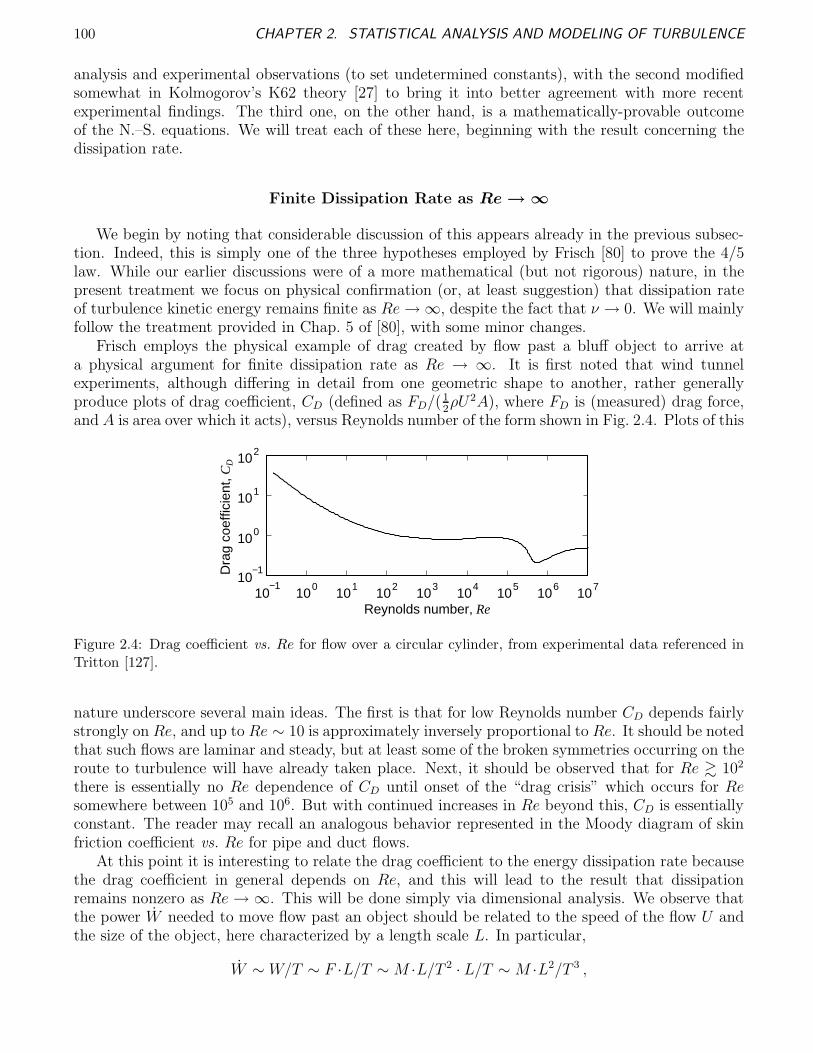
100 CHAPTER 2. STATISTICAL ANALYSIS AND MODELING OF TURBULENCE
analysis and experimental observations (to set undetermined constants), with the second modifiedsomewhat in Kolmogorov’s K62 theory [27] to bring it into better agreement with more recentexperimental findings. The third one, on the other hand, is a mathematically-provable outcomeof the N.–S. equations. We will treat each of these here, beginning with the result concerning thedissipation rate.
Finite Dissipation Rate as Re → ∞
We begin by noting that considerable discussion of this appears already in the previous subsec-tion. Indeed, this is simply one of the three hypotheses employed by Frisch [80] to prove the 4/5law. While our earlier discussions were of a more mathematical (but not rigorous) nature, in thepresent treatment we focus on physical confirmation (or, at least suggestion) that dissipation rateof turbulence kinetic energy remains finite as Re → ∞, despite the fact that ν → 0. We will mainlyfollow the treatment provided in Chap. 5 of [80], with some minor changes.
Frisch employs the physical example of drag created by flow past a bluff object to arrive ata physical argument for finite dissipation rate as Re → ∞. It is first noted that wind tunnelexperiments, although differing in detail from one geometric shape to another, rather generallyproduce plots of drag coefficient, CD (defined as FD/(1
2ρU2A), where FD is (measured) drag force,
and A is area over which it acts), versus Reynolds number of the form shown in Fig. 2.4. Plots of this
Dra
g co
effic
ient
, CD
10−1
100
101
102
10−1
100
101
102
103
104
105
106
107
Reynolds number, Re
Figure 2.4: Drag coefficient vs. Re for flow over a circular cylinder, from experimental data referenced inTritton [127].
nature underscore several main ideas. The first is that for low Reynolds number CD depends fairlystrongly on Re, and up to Re ∼ 10 is approximately inversely proportional to Re. It should be notedthat such flows are laminar and steady, but at least some of the broken symmetries occurring on theroute to turbulence will have already taken place. Next, it should be observed that for Re & 102
there is essentially no Re dependence of CD until onset of the “drag crisis” which occurs for Resomewhere between 105 and 106. But with continued increases in Re beyond this, CD is essentiallyconstant. The reader may recall an analogous behavior represented in the Moody diagram of skinfriction coefficient vs. Re for pipe and duct flows.
At this point it is interesting to relate the drag coefficient to the energy dissipation rate becausethe drag coefficient in general depends on Re, and this will lead to the result that dissipationremains nonzero as Re → ∞. This will be done simply via dimensional analysis. We observe thatthe power W needed to move flow past an object should be related to the speed of the flow U andthe size of the object, here characterized by a length scale L. In particular,
W ∼ W/T ∼ F ·L/T ∼ M ·L/T 2 · L/T ∼ M ·L2/T 3 ,
2.2. THE KOLMOGOROV THEORY OF TURBULENCE 101
where F is force; M is mass, and T is time. We observe that W has units mass times rate of viscousdissipation and also can be related to the drag coefficient as
W ∼ CDρL2U3 .
To see this, observe that by definition
CD =FD
1
2ρU2
.
At the same time
W = FD L =1
2ρU2ALCD , ⇒ W = W/T =
1
2ρU3ACD ∼ CDρL2U3 .
The dissipation rate is generally written per unit mass; in particular, we recall that ε ∼ L2/T 3.Thus, we write
ε ∼W
ρL3∼ CD
U3
L,
by equating ε to power per unit mass. Now recall from Fig. 2.4 that at high Re when a flow shouldbe turbulent, CD is independent of Re, and hence ε is independent of viscosity for Re → ∞. Thisprovides an heuristic demonstration of the following (as appears in [80]):
Finite dissipation. If, in an experiment on turbulent flow, all control parameters are held constantexcept for viscosity, which is lowered as much as possible, the energy dissipation per unit massde/dt ∼ ε behaves in a way consistent with a finite positive limit.
The 2/3 Law
We begin by stating Kolmogorov’s 2/3 law as given by Frisch [80]. We follow this with a specificformula corresponding to the statement, and finally show how the well-known k−5/3 energy spectrumfollows directly from this formula. We emphasize from the start that these are mainly empiricalresults, and the reader is encouraged to consult Chap. 5 of [80] to see specific comparisons withexperimental data. The 2/3 law can be stated as follows (Frisch [80]):
Kolmogorov’s 2/3 law. In a turbulent flow at very high Reynolds number, the mean-squarevelocity increment 〈(δu(ℓ))2〉 between two points separated by a distance ℓ behaves approximately asthe two-thirds power of the distance.
Several remarks are in order for interpretation of this result. First, we should observe that (δu)2
is a (squared) magnitude of the vector quantity δu, so one might question whether any sense canbe made of this unless the turbulence is isotropic. But it turns out that this same scaling seems tohold for individual components of velocity increments, independent of isotropy (see experimentalresults presented in Chap. 5 of [80]). Of more importance is the length ℓ. We would expectfrom hypotheses discussed in preceding subsections that ℓ should be very much smaller that theintegral scale. Indeed, the 2/3 law holds specifically in the inertial subrange of the energy spectrumcorresponding, roughly, to Taylor microscale lengths as we have previously discussed in connectionwith Fig. 1.5. Finally, the “very-high Reynolds number” aspect of the statement of this law is veryimportant. For low Re (but still high enough to be turbulent) the range of ℓ over which the 2/3law holds is very small; but as Re increases this range increases. We again remind the reader ofdiscussions associated with Fig. 1.5 where it was argued that this type of behavior is predicted, atleast qualitatively, from the Galerkin form of the N.–S. equations.
102 CHAPTER 2. STATISTICAL ANALYSIS AND MODELING OF TURBULENCE
We can now provide a formula corresponding to the 2/3 law. To do this we first recognize that〈(δu(ℓ))2〉 is actually the second-order structure function of u defined in general in Eq. (1.22). Thatis,
S2(ℓ) = 〈(δu(ℓ))2〉
= 〈(u(x + ℓ) − u(x))2〉 .
It is useful to note, as we have earlier, that in the context of velocity components S2 is clearly relatedto kinetic energy, and that in general it is associated with “energy” in the sense of L2 functions.
We next recall the meaning of the inertial subrange as given in Def. 1.77; that is, this is the rangeof scales over which viscosity is unimportant—viscous forces are dominated by inertial forces. Inparticular, this corresponds to Re sufficiently high that at low to moderate wavenumbers diffusiveeffects are completely dominated by advective effects in the N.–S. equations. We should recallthat this would correspond to Kolmogorov’s second universality assumption for which turbulencestatistics depend only on the length scale ℓ and the dissipation rate ε. Now because S2 is associatedwith kinetic energy, it must have general dimensions L2/T2. Also, we know that ε ∼ L2/T3, andwe want to find a combination of ℓ and ε that has the dimensions of energy. It is thus easily seenthat the only possible combination of these variables is
S2(ℓ) = Cε2/3ℓ2/3 , (2.92)
where C is a universal constant.There are two main consequences that can be readily deduced from the 2/3 law. The first is the
form of the turbulence kinetic energy spectrum, and a second lesser-known one is the exponent h inthe Frisch’s Hypothesis 2 regarding self similarity of N.–S. turbulence. We will treat each of thesein the following two subsections.
The k−5/3 energy spectrum. We can now use Eq. (2.92) to derive the widely-quoted Kolmogorovk−5/3 inertial-range scaling of the turbulent energy spectrum. To do this we first observe that S2
in Eq. (2.92) is expressed in physical space, and we will denote this as E as a reminder that it isenergy. Thus, we write
E = Cε2/3ℓ2/3 , (2.93)
But what is needed is a function of the wavenumber k. Clearly, we should be able to express anincremental part of E in Fourier space as dE = E(k)dk. From this it follows that the small-scaletotal (cumulative) energy corresponding to all wavenumbers higher than an arbitrary (but evidentlychosen in the inertial subrange) one k must be
E(k) =
∫ ∞
k
dE =
∫ ∞
k
E(k)dk .
It is shown in [80], under rather general circumstances, that E(k) must satisfy
E(k) ∝ k−n , 1 < n < 3 , (2.94)
and substitution of this into the integral on the right-hand side above leads to
E(k) ≃
∫ ∞
k
k−n dk
= −1
1 − nk−n+1
≃ −1
1 − nE(k)k .
2.2. THE KOLMOGOROV THEORY OF TURBULENCE 103
We remark that the estimate of E(k) given in the relation (2.94) is consistent with velocity beingat least in L2, so it is a mathematically-reasonable assertion.
Now observe that the range of n given above guarantees that
Cn ≡ −1
1 − n> 0 ,
and since k is arbitrary we can write E(k) = CnE(k)k for any k. Finally, we note that up to ascaling constant (that depends on details of basis functions chosen for a Fourier representation) wehave k = 1/ℓ, so from Eq. (2.93) we obtain
CnE(k)k = Cε2/3k−2/3 ,
and rearrangement leads to Kolmogorov’s well-known result for the inertial range energy spectrum,
E(k) = CKε2/3k−5/3 , (2.95)
where CK is the Kolmogorov constant. This constant must be determined from experimental mea-surements, and it appears not to be truly constant with observed values generally in the range fromunity to two (see, e.g., Chasnov [128]).
We remark, as noted in [80], that Kolmogorov did not actually present this result in his 1941papers. Rather, it was first given by Obukhov [129] in 1941. Furthermore, because the Russiantechnical literature was not widely available in the West until considerably later, this same resultwas independently discovered by several other researchers during the mid to late 1940s.
The scaling exponent h. There is yet another result that can be easily deduced from the 2/3 law.Recall that in Frisch’s second hypothesis it was assumed that velocity increments are self similaron small scales, and that there is a unique scaling exponent h which was not specified at that time.The 2/3 law permits us to determine the value of this exponent.
From Eq. (2.90) we haveδu(x, λℓ) = λhδu(x, ℓ) ,
which we write in terms of the second-order structure function as
S2(λℓ) = 〈(δu(x, λℓ))2〉 = Cε2/3(λℓ)2/3 .
But by (2.90) this must beλ2h〈(δu(ℓ))2〉 = Cε2/3λ2/3ℓ2/3 .
Thus, it follows that the unique scaling exponent has the value h = 1/3. We remark that while thisderivation would appear to require isotropy, Frisch [80] notes that there is an alternative derivationthat does not require this.
The 4/5 Law
The 4/5 law, although probably less quoted and possibly less directly useful than the 2/3 law,is in many respects the most important of the K41 results. This is true for two main reasons.First, it is derived directly from the N.–S. equations (albeit, with the use of a number of restrictiveassumptions), and unlike the 2/3 law it contains no adjustable constants—it is the only exact resultfor the Navier–Stokes equations at high Re. Second, and equally important, it has been validatedin numerous laboratory experiments. The 4/5 law proposes that third-order structure functions ofvelocity increments scale linearly with separation distance ℓ. More precisely, we have the following:
104 CHAPTER 2. STATISTICAL ANALYSIS AND MODELING OF TURBULENCE
Kolmogorov’s 4/5 law. In the limit of infinite Reynolds number, the third-order longitudinalstructure function of homogeneous isotropic turbulence, evaluated for increments ℓ small comparedwith the integral scale, is given in terms of the mean energy dissipation rate per unit mass as
S3‖(ℓ) = −4
5εℓ . (2.96)
Derivation of this exact result is lengthy and nontrivial, and we will not present it here. (Theinterested reader should consult Chap. 6 of [80].) We simply observe that the derivation providedin [80] requires three conditions: homogeneity, isotropy and fully-developed turbulence. We havenot previously emphasized the last of these, so we will provide a few additional remarks here. Wefirst recall from Def. 1.72 that this terminology implies high-Re turbulence in which statistics areno longer changing in the flow direction. Thus, we see that within the context of the other tworequirements, the only thing added by requiring fully-developed turbulence is the specific statementof high Re (as given in the 4/5 law). Hence, this has in part been implied by all of our precedinghypotheses and is basically subsumed by the homogeneity and isotropy requirements. The specificinformation employed by Frisch [80] to prove Eq. (2.96) is the following:
i) energy is input only on large scales;
ii) the N.–S. solutions tend to a stationary state at large times, and
iii) mean dissipation rate ε remains finite as Re → ∞.
Moreover, it is emphasized that the self similarity of Frisch’s Hypothesis 2 stated earlier is not used.With this combination of hypotheses and their consequences, it is possible to derive the followingthird-order ODE for S3 forced by ε:
(1 + ℓ
d
dℓ
)(3 + ℓ
d
dℓ
)(5 + ℓ
d
dℓ
)S3(ℓ)
6πℓ= −12ε . (2.97)
The unique, exact solution to this equation is given in Eq. (2.96) for the longitudinal case.
Higher-Order Structure Functions
Finally we note that Hypothesis 2 suggests that structure functions of arbitrary (but finite)order p should scale as
Sp(ℓ) = Cpεp/3ℓp/3 , (2.98)
where the Cps are dimensionless and independent of Re. It is clear that when p = 2 we recover the2/3 law with C2 = CK , and when p = 3 we obtain the 4/5 law with C3 = −4/5. We remark thatexperimental evidence for the validity of Eq. (2.98) for large p is not strong. It is believed that thisdiscrepancy is related to intermittency, effects of which have not been included in the K41 theory(but attempts at this were made in the K62 theory), and there is still considerable ongoing researchrelated to this. We refer the reader to [80] and references therein for more details on this importantand interesting topic.
2.3 Summary
This chapter has been devoted to statistical analysis and modeling of Navier–Stokes turbulence.We began with a fairly detailed treatment of the Reynolds-averaged Navier–Stokes equations. This
2.3. SUMMARY 105
included analysis of the Reynolds decomposition and of the RANS equations, independent of anyspecific modeling procedures. The key results of this were i) the Reynolds decomposition imposesan extremely difficult modeling task because essentially all flow details most be modeled—usingstatistical quantifications; and ii) the form of the RANS equations is such that their solutions cannever converge to time-averaged solutions to the N.–S. equations except in the case of availabilityof exact Reynolds stresses—which can be obtained only via DNS.
We next described three main widely-used classes of RANS models: i) mixing-length theory,ii) k–ε models and iii) second-moment closures. It was clear that none of these is well foundedin either physics or mathematics; so the generally poor results they produce comes as no surprise,and as a consequence they cannot be used as predictive tools. On the other hand, in the presenceof sufficient data required for detailed calibration of closure constants and validation of results,it is possible to use such models in an interpolatory fashion—of course, with caution. They aresometimes able to at least mimic observed physical trends, but they are essentially never able toaccurately reproduce entire flow fields. This, again, is a completely expected outcome—too muchinformation has been lost in the averaging process to be able to recover it by anything short ofexact statistical correlations (the Reynolds stresses).
Finally, we presented a brief treatment of the Kolmogorov K41 theory. We emphasized that thisis also a statistical treatment of the N.–S. equations, but it is intrinsically different from Reynoldsaveraging in that the (implied) decomposition of flow variables is a Hilbert-space decomposition.Furthermore, no modeling, per se, is contained in the Kolmogorov results; on the other hand, ratherrestrictive assumptions must be imposed to obtain them. There are three main results: i) finitedissipation rate as Re → ∞, ii) the 2/3 law, and iii) the 4/5 law. The first two of these are mainlyempirical but can be derived on the basis of dimensional analysis. The second of these leads totwo further results—the k−5/3 energy spectrum of the inertial subrange, and a value h = 1/3 fora universal scaling constant associated with self similarity on small scales. The last of the keyresults, the 4/5 law, is directly derivable from the N.–S. equations under the hypotheses of high-Rehomogeneous isotropic turbulence. It is exact (no adjustable constants), nontrivial and in goodagreement with experimental data. It is the only such result known up to the present time.

106 CHAPTER 2. STATISTICAL ANALYSIS AND MODELING OF TURBULENCE
Chapter 3
Large-Eddy Simulation and Multi-Scale
Methods
In the preceding chapter we provided an overview of RANS methods that demonstrated theirinability to produce solutions to the N.–S. equations. This is obviously a very serious shortcomingof any turbulence modeling procedure, and although it has certainly been recognized for a long timeby theorists, especially mathematicians, it has had little, if any, impact on engineering analyses ofturbulence. On the other hand, failures of RANS methods are so widespread that engineers havesought other techniques from the earliest that computers have been available. Large-eddy simulation(LES) was the first of these, proposed by Smagorinsky [130] in 1963 and by Deardorff [10] in 1970,and actually preceded both modern k–ε models and SMCs.
In this chapter we will present a fairly thorough overview of the main aspects of LES, particularlywith regard to subgrid-scale (SGS) models, and to a lesser extent the problem of filtering thegoverning equations. But in addition we will propose viewing LES as a subset of the much widerclass of multi-scale methods (see e.g., E and Engquist [131], and references therein) and showthat it, in a sense, represents a link between classical turbulence modeling procedures and newapproaches (such as DNS) that emphasize the dynamical systems aspects of the N.–S. equations.We will establish this link by first providing a fairly detailed treatment of LES, then presentingdetails of the dynamical systems view of the N.–S. equations, a la Ruelle and Takens [8], and finallyshowing how this relates to multi-scale methods in general and LES in particular. We will thenconclude the chapter with a somewhat altered form of LES that explicitly utilizes this dynamicalsystems viewpoint for construction of SGS models and at the same time employs multi-scale ideasto combine the large and small scales.
3.1 Large-Eddy Simulation
In Chap. 1 we briefly discussed large-eddy simulation decomposition of dependent variables andfurther described LES as a turbulence computation method lying somewhere between RANS andDNS. But these discussions were mainly qualitative; here we will provide considerably more detail.We begin with a more thorough discussion of just where LES lies on the spectrum of turbulencemodels. Following this we review material presented earlier on the LES decomposition, and wecarry out the formal procedure for applying LES to the N.–S. equations, just as we have previouslydone in the RANS case. This process will include two specific aspects of crucial importance to LES:filtering the governing equations, and construction of SGS models. It is the specific approach usedfor each of these that allows distinctions to be made amongst the various forms of LES, and we willconsider several of the currently most widely used of these.
107

108 CHAPTER 3. LARGE-EDDY SIMULATION AND MULTI-SCALE METHODS
3.1.1 Comparison of DNS, LES and RANS methods
We have already emphasized in Chap. 1 that in the context of turbulent flow simulations DNSrequires no modeling, and RANS approaches entail extensive modeling, as we have seen in Chap.2. The former simply exploits numerical analysis to construct an efficient implementation of anappropriate N.–S. solution procedure. No physical assumptions need be made beyond those alreadyembodied in the N.–S. equations themselves; but because of the extremely wide range of length andtime scales, reflected in the magnitude of the Reynolds number, it is not yet possible to performsuch calculations if Re is at all large. The reader will recall in Chap. 1 we argued that the totalrequired arithmetic scales as Re3 for DNS calculations, and this is an optimistic estimate. It is oftenpointed out that at the current rate of improvement in computing hardware, this translates to beingable to double the size of Re in a calculation only once in a five to ten year period. Clearly, this iscompletely unacceptable from a practical standpoint as is especially obvious when it is consideredthat Re∼O(104) is the current state of the art.
Until recently, the only alternatives have been RANS methods. In these required arithmetic isnearly independent of Re, and in fact many such methods work best at very high Re where scaleseparation is more likely to be a reasonable approximation. But as we have seen, no RANS approachcan be predictive due to the extensive modeling requirements; so this too is unacceptable.
The same type of analysis leading to the Re3 arithmetic requirement for DNS shows that totalarithmetic required for LES should not exceed Re2. In particular, the goal in LES is to directlysimulate only into the inertial subrange, and not all the way to the dissipation scales as must be donein DNS. At the same time we see that the LES models need represent only the high-wavenumberpart of the inertial subrange, and the dissipation scales—in sharp contrast with RANS models whichare formally required to model everything from (at least) the integral scales through the dissipationrange.
Furthermore, we know the Taylor microscales lie fairly deep within the inertial subrange, and it
was shown in Chap. 1 that ℓ/λ ∼ Re1/2ℓ , where ℓ is the integral scale length, and λ is the Taylor
microscale length. Thus, in 3D the ratio of largest to smallest scales that must be resolved is
proportional to Re3/2ℓ , and as we did in the context of DNS estimates we assume the numerical time
step sizes should satisfy a Courant condition; so the total arithmetic is ∼Re2 for LES provide SGSmodel evaluation is independent of Re, which usually is the case. Unlike the DNS case for which Re3
is actually somewhat optimistic, the Re2 estimate for LES is likely to be somewhat conservative,and one sometimes finds predictions of total arithmetic as low as Re3/2. But even the Re2 estimateis beginning to be an acceptable amount of arithmetic on modern computing machinery, and LES isnow an available option in many commercial CFD software suites intended for practical engineeringapplications.
We can summarize these comparisons as follows:
i) DNS requires no modeling, but it demands resolution from the large scales all the way throughat least the beginning of the dissipation scales. This results in total arithmetic scaling at leastas Re3, or worse.
ii) LES requires modeling of part of the inertial subrange and into the beginning of the dissipationscales. The amount of required modeling is set by the amount of resolution that can beafforded, but it is unlikely that total arithmetic will scale worse than Re2.
iii) RANS requires modeling of everything from the integral scales into the dissipation range—only mean (zeroth-mode) quantities are directly computed. As a consequence, total arithmeticis at most a weak function of Re.
3.1. LARGE-EDDY SIMULATION 109
In addition, we remark here (and we will demonstrate this in detail later) that in contrast toRANS, it can be shown that LES procedures generally converge to DNS (and thus their solutionscan be expected to converge to N.–S. solutions) as discretization step sizes (and filter widths) arerefined.
Finally, before proceeding to details, it is worthwhile to mention that just as is true for RANSmethods, there are by now many different forms of LES. We will not here attempt a detailedtreatment of all of these but instead concentrate on a few of the better-known and more widely-used approaches. The oldest, but yet still widely used, is the Smagorinsky model [130], with “model”referring to treatment of the unresolved stresses. We will later see that this approach in not verydifferent from mixing-length models used in RANS methods, and this is not surprising since earlywork with LES was actually done in the shadow of RANS theory. Like mixing-length models,the Smagorinsky model works well only for a very limited number of flow situations, and the firstattempts to correct this resulted in what are now termed “scale-similarity” models, first proposed byBardina et al. [132]. These were not successful in general, and the next “bandaid” consisted of theso-called “dynamic” models introduced by Germano et al. [68]. Both of these approaches tend to betoo little dissipative (although this can be corrected in the latter), in contrast to the Smagorinskymodel which is essentially always overly dissipative. The natural response to this conundrum was toeffectively “average” scale-similarity and more dissipative models such as Smagorinsky to produce“mixed” models. All of these methods have been constructed via the “classical” approach to LESconsisting of the following steps:
i) decompose flow variables into large- and small-scale parts, with the large-scale part purportedlydefined by a filtering process;
ii) filter the governing equations, and substitute the decomposition from part i) into the nonlinearterms to construct the unclosed terms to be modeled and obtain a system of equations forresolved-scale variables that is as close as possible to the N.–S. equations;
iii) model the unresolved stresses;
iv) solve equations for the large-scale contribution (while essentially ignoring the small-scale part).
With the exception of the last, we will treat these steps in detail in the sequel; but before doingthis we wish to emphasize that there are beginning to appear forms of LES that do not follow thisstandard formulation, and we will mention a few of these at this time and provide further detailsin the section devoted to multi-scale methods.
There are many different approaches being attempted, ranging from simply solving the governingequations with numerical methods that are strongly dissipative and thus replacing physical (actually,model) dissipation with numerical dissipation, to quite sophisticated procedures which attempt todirectly model the subgrid-scale variables. The former approaches are usually termed “implicit” LES(ILES), due to Fureby and Grinstein [133], an example of which is monotonically integrated LES(MILES), as first proposed by Boris et al. [134], while the latter comprise a wide class of methodsreviewed in some detail by Sagaut [73] and often called “synthetic velocity” approaches. Specificones of these include the linear-eddy models (LEMs) and one-dimensional turbulence (ODT) modelsof Kerstein and coworkers (see, e.g., Kerstein [135] and Echekki [71], respectively), the “estimation”models of Domaradzki and coworkers (e.g., Domaradzki and Saiki [70]) and the chaotic-map modelsof McDonough and coworkers (e.g., Hylin and McDonough [136], and the summary in [73]).
110 CHAPTER 3. LARGE-EDDY SIMULATION AND MULTI-SCALE METHODS
3.1.2 The LES decomposition
We earlier presented the LES decomposition in Eq. (1.27) for a generic scalar variable. Here, weconsider this in more detail for the velocity vector U = (u, v, w)T and begin by writing
U(x, t) = u(x, t) + u′(x, t) . (3.1)
We remind the reader of two key points associated with this form of decomposition. The first isthat ‘˜ ’ represents a spatial filter that should be considered a low-pass filter which, in principle,removes all wavenumbers in the Fourier representation of U above those supported by the chosendiscretization of the governing equations. Formally, we have
U(x, t) =
∫
Ωi
G(x|ξ) U(ξ, t) dξ ≡ u(x, t) , (3.2)
where the filter kernel G is often taken to be a Gaussian, and Ωi is a subdomain of the solutiondomain Ω such that the volume of Ωi is approximately h3 with h being the discrete step size of thenumerical approximation. We remark that there is an alternative interpretation of this. Namely, wemight instead take the domain of integration to be the entire problem solution domain Ω and thendemand that G have compact support over just a few multiples of h (in each direction). Clearly,this is equivalent to our notation. In addition, it is probably more precise to measure this supportin terms of the “filter width,” usually denoted ∆, which itself is a few multiples of h in length.
The second point, which follows from the first, is that u′(x, t) is a very different mathematicalobject from that possessing the same notation in RANS formalisms. Indeed, we see that u′ is thehigh-pass filtered part (or, remainder in the Fourier series context) of the solution U (x, t) after thelow-pass filtering of Eq. (3.2) has been applied. That is,
u′(x, t) = U(x, t) − u(x, t) , (3.3)
which formally has exactly the same appearance as the RANS result. But due to the nature of theLES decomposition the are obvious consequences of this formalism that differ from the RANS case,namely,
˜u(x, t) 6= u(x, t) and u′ (x, t) 6= 0 , (3.4)
except in the special case of a projective filter. In particular, from Eq. (3.3) we have
u′ (x, t) = U(x, t) − ˜u(x, t)
= u(x, t) − ˜u(x, t)
6= 0 ,
since in general,
˜u(x, t) =
∫
Ωi
G(x|ξ) u(ξ, t) dξ 6=
∫
Ωi
G(x|ξ) U(ξ, t) dξ = u(x, t) ,
for typical (non-projective) filter kernels. We remark that a specific exception to this is the sharp-cutoff Fourier-space filter which is projective.
As we have previously noted, the form of Eq. (3.1) is suggestive of a Hilbert-space decompositionexcept, as already indicated, the subspaces are not perfectly orthogonal. Despite this technicality,it is useful to identify (3.1) with the Fourier representation
U(x, t) =
kc∑
|k|≥0
ak(t)ϕk(x) +
∞∑
|k|=kc+1
ak(t)ϕk(x) . (3.5)

3.1. LARGE-EDDY SIMULATION 111
In this manner it is easy to provide an heuristic (but not rigorous) argument for convergence of LESsolutions to solutions to the N.–S. equations. In particular, in contrast to a RANS decompositionin which significant information may be lost in a nonrecoverable way due to the simple averagingprocedure employed, Eq. (3.5) representing LES shows that as discrete resolution is increased (kc →∞), the computed result should converge to the true function being represented (assuming, of course,that the function is at least in L2(Ω)).
3.1.3 Derivation of the LES filtered equations
In this section we will derive the filtered equations employed in the LES formalism. We begin withconservation of mass, which in the incompressible case treated here is extremely simple, and wethen proceed to the more tedious momentum equations; viz., we follow the same process introducedin treatment of the RANS equations in the preceding chapter.
The Continuity Equation
Conservation of mass, or the continuity equation, for an incompressible flow is just the divergence-free condition ∇·U = 0, or
ux + vy + wz = 0 (3.6)
in 3D. Formal application of the filter results in
ux + vy + wz = 0 .
We see that to obtain the desired form will require commutativity of the spatial filter and spatialdifferentiation. For example, the first term in the above is of the form
∫
Ωi
G(x|ξ)∂u
∂ξ(ξ, t) dξ .
It should be clear that commutativity will not hold for all possible kernels G, but the typical onesused for LES filters usually possess arguments of the form x − ξ, and they generally have (nearly)compact support on Ω. In this case it can be shown that ux = ux, etc., at least in Cartesiancoordinate systems. We leave demonstration of this for the reader. Thus, Eq. (3.6) can be replacedwith
ux + vy + wz = 0 , (3.7)
or ∇·u = 0.At this point it is worthwhile to again recall that u is a low-pass filtered quantity associated
with the first few terms of a Fourier representation of U as given in Eq. (3.5). Thus, ∇·U = ∇·uby definition. Then it follows that
0 = ∇·U = ∇·(u + u′) .
But ∇· u = 0 also holds as seen from Eq. (3.7). Hence, just as was the case for the Reynoldsdecomposition, we see that
∇·u′ = 0 . (3.8)
We again recall from our Galerkin representation of the Navier–Stokes equations in Chap. 1 thatin Fourier space this must hold on a mode-by-mode basis; but we see that even in the absence ofa projective filter the divergence-free condition must hold separately on large and small scales, andin synthetic-velocity SGS models this requirement should be explicitly enforced.
112 CHAPTER 3. LARGE-EDDY SIMULATION AND MULTI-SCALE METHODS
The Momentum Equations
From the preceding straightforward exercise in filtering the continuity equation we can easilydeduce the filtered form of the momentum equations. These can be expressed as
∂u
∂t+ ∇·
(UU
)= −∇p + ν∆u . (3.9)
Obtaining the first term on the left-hand side involves a trivial (assuming time-independent coordi-nates) commutativity of the filter with the temporal derivative, while both terms on the right-handside follow in the same way as in the continuity equation. Thus, just as was true with Reynoldsaveraging, filtering of the momentum equations leads to significant difficulty only in the nonlinearterms (provided simple filters with properties as we have been supposing here are employed). Aswill be clear as we proceed, the difficulties associated with the nonlinear terms are similar to (butmore complicated than) those arising in the RANS case, and in generalized coordinates they occurfor linear terms as well.
For the nonlinear terms we introduce the LES decomposition Eq. (3.1) and write
∇·(UU
)= ∇·
(︷ ︸(u + u′) (u + u′)
).
︷ ︸(u + u′) (u + u′) =
︷ ︸(u + u′) (u + u′)
︷ ︸(u + u′) (v + v′)
︷ ︸(u + u′) (w + w′)
︷ ︸(u + u′) (v + v′)
︷ ︸(v + v′) (v + v′)
︷ ︸(v + v′) (w + w′)
︷ ︸(u + u′) (w + w′)
︷ ︸(v + v′) (w + w′)
︷ ︸(w + w′) (w + w′)
. (3.10)
We examine one component of this tensor in detail to deduce the structure induced by decom-position and filtering. Consider
︷ ︸(u + u′) (v + v′) = ˜u v + ˜uv′ + ˜vu′ + u′v′ . (3.11)
We observe that there are three specific types of terms in this expression, and in all of the analogous
ones corresponding to the remaining components of Eq. (3.10). The first of these, ˜u v (a part ofwhat is known as the Leonard stress), would have simply been of the form u v in a Reynolds-
averaging procedure. On the other hand, despite its greater complexity, ˜u v still can be computeddirectly (without any modeling required) since we have equations for u and v.
The second pair of terms, ˜uv′ + ˜vu′ , is known as the cross stress, and this would be identicallyzero in a Reynolds-averaging formalism. In the present context, however, these terms are not onlynonzero, but they must be modeled because they contain small-scale factors.
Finally, terms of the form u′v′ are analogous to components of the Reynolds stress tensor thatoccurs in RANS procedures, and they are usually called Reynolds stresses even in the LES context.In usual treatments of LES, the terms on the right-hand side of Eq. (3.11) are expressed in Cartesiantensor notation as given here parenthetically:
Lij ≡ ˜u v − u v(= ˜ui uj − ui uj
), (Leonard stress)
Cij ≡ ˜uiu′j + ˜uiu
′j
(= ˜uiu
′j + ˜uiu
′j
), (cross stress)
Rij ≡ u′v′(= u′
iu′j
), (Reynolds stress)

3.1. LARGE-EDDY SIMULATION 113
where the origin of the second term in the Leonard stress will be made clear below.It is important to recognize that the last of these terms are fundamentally different from the
Reynolds stress components arising in RANS formalisms, despite their common name. In particularwe should recall that the individual fluctuating quantities appearing in the usual Reynolds stresstensor contain information from all but the zeroth mode of their Fourier representations (recall Eq.(2.23)), while the subgrid part of a LES representation is associated with a high-pass filtering ofthe solution, thus carrying information only from the modes above some cut-off wavenumber kc
corresponding to what can be supported by the discretization employed in treating the filtered,large-scale equations. Furthermore, it should again be observed that, for example, u′ = 0 in
RANS formulations; but u′ 6= 0 in the LES case, as we have already stressed. In short, at least
from a fundamental mathematical viewpoint we must expect that u′v′ and u′v′ are quite different,
and in particular we should not expect u′v′ = u′v′ in general, although they have been given thesame nomenclature and notation. On the other hand, due to presence of the Leonard stress, theoverall SGS stresses may not differ significantly from the corresponding Reynolds stresses of RANSapproaches aside from their time dependence.
We remark that in early treatments of SGS modeling each of the contributions listed above wasmodeled separately; since they correspond to different parts of the energy spectrum one could arguethat this should be an advantage. On the other hand, it is shown by Sagaut [73] that for typicalsimple filters (but not for all filters) the invariance properties of the N.–S. equations are preservedunder filtering, but in contrast, the individual parts of the LES decomposition do not all separatelypreserve all invariances. In particular, neither Leonard nor cross stresses are Galilean invariant, buttheir sum is; hence, the complete SGS stress is Galilean invariant. This, however, suggests that atleast from the standpoint of maintaining N.–S. invariances, it is probably best to model SGS stressas a single entity. This is now the usual practice. Beyond this is the additional fact that unlessexplicit time integrations are employed for the advective terms, an iteration process is required forconstruction of Leonard and cross stresses at each time step, although this might be incorporatedin the nonlinear iterations of an implicit scheme in any case.
We also note that more elaborate filters can result in loss of invariance of the filtered equa-tions themselves. Specific examples include those with different filter lengths in different directionsand those having variable filter lengths in any, or all, direction(s). Such difficulties suggest thatalternatives to filtering the governing equations should possibly be sought.
We now observe that the filtered momentum equations still are not yet in a useful form. Toobtain such a form we recognize that what is needed for the nonlinear term on the left-hand side ofEq. (3.9) is ∇·(uu). But we have seen that this form does not occur in the analysis of the filterednonlinear term (except in the Leonard stress where it was apparently added artificially). Thus, theonly choice for obtaining what is needed is to add and subtract this term from the left-hand sideof Eq. (3.9). Once this is done, we replace the filtered nonlinear terms on the left-hand side of Eq.(3.10) with
uu +
[︷ ︸(u + u′) (u + u′)−uu
]≡ uu + τ
SGS,
where τSGS
is notation for the LES subgrid-scale stress. We now can write Eq. (3.9) as
ut + ∇·(uu) = −∇p + ν∆u −∇·τSGS
, (3.12)
withτ
SGS,ij≡ Lij + Cij + Rij . (3.13)
This is the equation for the large- (resolved-) scale part of a LES formulation. We observe thatonly τ
SGSneeds to be modeled, and in that sense Eq. (3.12) takes on the same appearance as would a
114 CHAPTER 3. LARGE-EDDY SIMULATION AND MULTI-SCALE METHODS
time-dependent RANS method. But in viewing (3.12) in this context we emphasize that presence ofthe time-derivative term in Eq. (3.12) is rigorously correct—in contrast to the RANS case. Namely,the LES decomposition is such as to retain time dependence in both large and small scales becausetemporal averaging has been replaced with spatial filtering in the construction process. We willalso see in the next section that models of τ
SGShave, from the beginning, usually been constructed
such that τSGS
→ 0 as h → 0 (or kc → ∞), where h is a measure of discretization step sizes. Thus,it is clear that Eq. (3.12) converges to the N.–S. equations in this limit for such models, and as wehave previously noted, LES→DNS. We again emphasize that such features are not part of RANSmodeling. Indeed, the mathematical nature of the Reynolds decomposition precludes this.
Finally, we note that −∇· τSGS
is typically modeled in a way reminiscent of the Boussinesqhypothesis, so one might argue that all that is actually accomplished with it is stabilization of thenumerical algorithms being employed to solve an under-resolved discretization of Eq. (3.12)—i.e.,increased (numerical) dissipation. In fact, from a mathematical viewpoint, the only reason for fil-tering is to eliminate aliasing arising from under resolution imposed by coarse grids of practicaldiscretizations. While it should be clear that filtering U , itself, might be more appropriate in thiscontext, presence of the term −∇·τ
SGSis analogous to the artificial dissipation schemes widely em-
ployed for shock capturing in compressible flow simulations (see, e.g., Hirsch [137]). It is recognitionof this that suggests use of ILES-like procedures, but in light of this we expect such methods toperform poorly in situations for which the Boussinesq hypothesis is inadequate, and inparticular,when scale separation does not hold.
3.1.4 Subgrid-scale models for LES
As we have already suggested, there are many different forms of LES models, and we shall notattempt to treat more of than a few of the better known of these in the present lectures. In the firstsubsection we will introduce the basic Smagorinsky model [130] and discuss some of its advantagesand disadvantages. This will motivate considering two other types of models, the dynamic modelsand mixed models, in subsequent subsections.
The Smagorinsky model
The Smagorinsky model is the oldest of LES SGS models, but because of its simplicity it is stillwidely used. It is not a particularly good choice for wall-bounded shear flows, but for flows farfrom solid boundaries it can be quite adequate, especially if the large scale is well resolved with thecut-off wavenumber lying fairly deep within the inertial subrange.
This model is based on the Boussinesq hypothesis employed extensively in RANS models andtakes the form
τSGS
= −2νSGS
S , (3.14)
where S is the usual large-scale strain-rate tensor, and νSGS
is the subgrid-scale eddy viscosity. InCartesian tensor index notation this is
τSGS,ij
= −2νSGS
Sij , i, j = 1, 2, 3, i 6= j .
The eddy viscosity is calculated using a formula analogous to the mixing-length formulation ofRANS methods:
νSGS
= (CS∆)2|S| . (3.15)
Here, ∆ is the filter width (proportional to grid spacing), and CS is the Smagorinsky “constant,”typical values of which are O(10−1); these can be estimated theoretically for isotropic turbulence(see [73] and references therein).
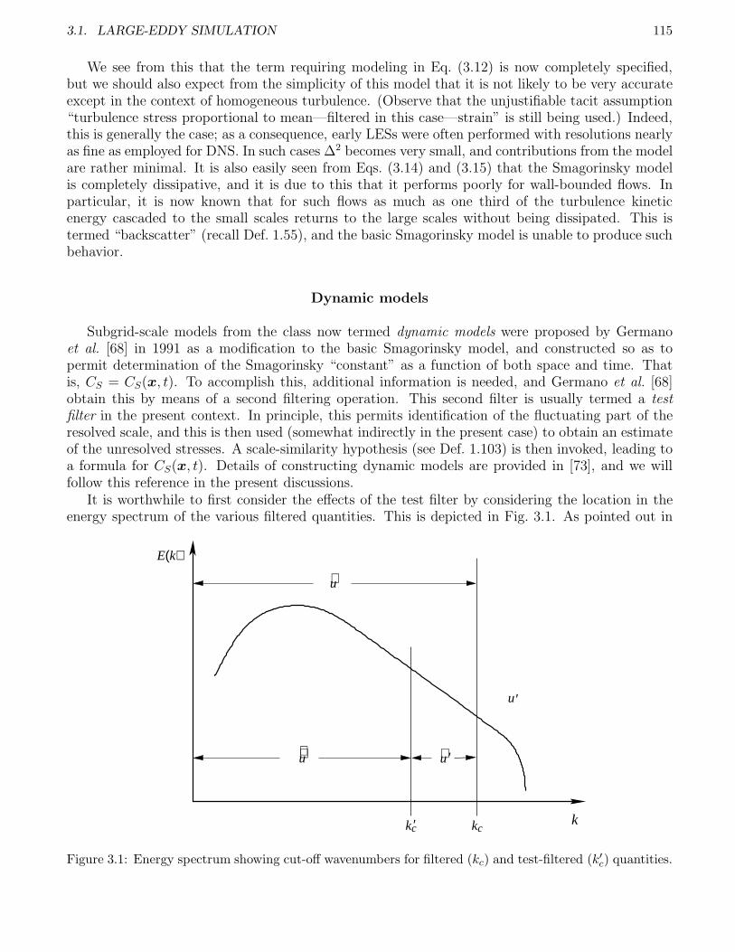
3.1. LARGE-EDDY SIMULATION 115
We see from this that the term requiring modeling in Eq. (3.12) is now completely specified,but we should also expect from the simplicity of this model that it is not likely to be very accurateexcept in the context of homogeneous turbulence. (Observe that the unjustifiable tacit assumption“turbulence stress proportional to mean—filtered in this case—strain” is still being used.) Indeed,this is generally the case; as a consequence, early LESs were often performed with resolutions nearlyas fine as employed for DNS. In such cases ∆2 becomes very small, and contributions from the modelare rather minimal. It is also easily seen from Eqs. (3.14) and (3.15) that the Smagorinsky modelis completely dissipative, and it is due to this that it performs poorly for wall-bounded flows. Inparticular, it is now known that for such flows as much as one third of the turbulence kineticenergy cascaded to the small scales returns to the large scales without being dissipated. This istermed “backscatter” (recall Def. 1.55), and the basic Smagorinsky model is unable to produce suchbehavior.
Dynamic models
Subgrid-scale models from the class now termed dynamic models were proposed by Germanoet al. [68] in 1991 as a modification to the basic Smagorinsky model, and constructed so as topermit determination of the Smagorinsky “constant” as a function of both space and time. Thatis, CS = CS(x, t). To accomplish this, additional information is needed, and Germano et al. [68]obtain this by means of a second filtering operation. This second filter is usually termed a testfilter in the present context. In principle, this permits identification of the fluctuating part of theresolved scale, and this is then used (somewhat indirectly in the present case) to obtain an estimateof the unresolved stresses. A scale-similarity hypothesis (see Def. 1.103) is then invoked, leading toa formula for CS(x, t). Details of constructing dynamic models are provided in [73], and we willfollow this reference in the present discussions.
It is worthwhile to first consider the effects of the test filter by considering the location in theenergy spectrum of the various filtered quantities. This is depicted in Fig. 3.1. As pointed out in
u∼∼
u∼
u′
u∼′
kckc′ k
E(k)
Figure 3.1: Energy spectrum showing cut-off wavenumbers for filtered (kc) and test-filtered (k′c) quantities.
116 CHAPTER 3. LARGE-EDDY SIMULATION AND MULTI-SCALE METHODS
[73] and elsewhere, it is typical for the filter width of the test filter to be double that of the basicfilter, so as indicated in the figure, the cut-off wavenumber corresponding to the test filter is lowerthan that of the original filter. This permits us to define
u′ = u − ˜u (3.16)
just as we defined u′ = U − u. Then invoking the scale-similarity hypothesis permits us to estimatestatistics of u′ (which are unknown) in terms of those of u
′ (which are known). We remark, however,that while this is what underlies the Germano et al. [68] dynamic model, the details are ratherdifferent. We outline these here, following Sagaut [73], and return to further direct application ofscale similarity in the next subsection.
The starting point for development of the dynamic model is a special case of the Germanoidentity [138], relating the Leonard stress to a similar twice-filtered tensor T and a second filteringof the usual SGS tensor. In particular, we have
Lij = Tij − τSGS,ij
, (3.17)
where analogous to Eq. (3.11) and following,
τSGS,ij
= Lij + Cij + Rij = UiUj − uiuj ,
Tij =˜UiUj − ˜ui
˜uj ,
Lij = ˜uiuj − ˜ui˜uj .
Proof of (3.17) is a direct calculation which we leave to the reader, and we omit it here. We note,however, the slightly altered form of Lij from that given earlier. This is a consequence of formallyseeking equations for the twice-filtered dependent variables.
We remark that in the context in which many of these quantities were originally introduced thetwo different filterings necessarily involved identical filters, but here the filters will be different. Inparticular, as already indicated the second, or test, filter will have filter width usually double that ofthe original filter. (Hence, the above formulas lead to nontrivial results even for projective filters.)
We next introduce the so-called deviatoric parts of the tensors τSGS,ij
and Tij , and at the sametime assume these can be modeled with analogous formulas employing the same closure constant.Then we can write
τdSGS,ij
≡ τSGS,ij
−1
3τSGS,kk
δij = CdSβij ,
T dij ≡ Tij −
1
3Tkkδij = Cd
Sαij .
We recall that τdSGS,ij
is simply τSGS,ij
with zero trace, as the Cartesian tensor operations indicate. It
should also be observed that employing the same value of CdS for both filter scales is analogous to
invoking a scale-similarity hypothesis.It should be observed that αij and βij are the SGS models with their closure constants removed.
βij = ∆2Sij|S| ,
and
αij = ∆2test˜Sij|
˜S| .
3.1. LARGE-EDDY SIMULATION 117
In the context of dynamic models the Smagorinsky model is most often, but not always, used.The reader should consult [73] to see other alternatives. We also note that with respect to theSmagorinsky model Cd
S is actually (CdS)2.
Analogous to the above relations we define the deviatoric part of the Leonard stress tensor anduse the above in the corresponding Germano identity:
Ldij ≡ Lij −
1
3Lkkδij = Cd
Sαij − CdSβij . (3.18)
Now recall that the whole point of the dynamic modeling process is to arrive at spatially andtemporally varying closure constants—Cd
S in the present case. But it is clear from Eq. (3.18) thatto proceed further we must employ the approximation
CdSβij = Cd
Sβij , (3.19)
which, as noted in [73], is equivalent to assuming CdS is constant over a subdomain corresponding
to the test filter width.One then seeks local values of Cd
S so that the error of approximation in (3.19) is minimized; thatis, we define
eij ≡ Lij −1
3Lkkδij − Cd
Sαij + CdSβij , i, j = 1, 2, 3 , (3.20)
the residual of (3.18) when (3.19) is used to replace CdSβij . It should be noted that this is a tensor
equation, implying that CdS, itself, is actually a tensor. In usual treatments of the dynamic modeling
approach, however, this is simplified by contraction with the strain-rate tensor Sij (Germano et al.[68]) or with the error itself (Lilly [139]). The former leads to difficulties at flow field locationswhere the strain rate is very small (or zero), so the latter is recommended. This is equivalent to theleast-squares problem of minimizing |e|2 with respect to Cd
S which leads to solving ∂|e|2/∂CdS = 0.
It is easily checked that the solution to this problem is
CdS =
mijLdij
mklmkl
, (3.21)
where mij = αij − βij , and we note that Einstein summation is being applied for repeated indices.As noted in [73], Cd
S given in Eq. (3.21) can exhibit two undesirable properties. First, it ispossible for Cd
S < 0 to hold, and in the context of the Smagorinsky model this implies a negativeSGS eddy viscosity. Since this is employed in the Boussinesq hypothesis, we see that the result isequivalent to a “backward heat equation”—a mathematically ill-posed formulation. But becausethis typically occurs at only a limited number of points on a computational grid it can be remediedby averaging, typically in directions in which the flow exhibits homogeneity, if such directions exist(see [73] for various options).
Moreover, proponents of dynamic models often view negative viscosities as a desirable feature(ignoring the basic bad mathematics they imply). In particular, the local (usually in both space andtime) solution instabilities resulting from ill posedness tend, in at least a qualitative way, to mimicthe backscatter that cannot be produced by the highly dissipative Smagorinsky model alone. Weshould again recall the Galerkin form of the N.–S. equations and observe that no Fourier modes aredamped, thus (from a numerical-analytic viewpoint) permitting unresolved high wavenumber effectsto alias the low-wavenumber behavior. But, of course, from a pure mathematical perspective, thisgrowth of Fourier coefficients is the hallmark of an ill-posed problem. Hence, it must be emphasizedthat despite the fact that this approach often produces approximately correct physical outcomes, itdoes so with completely incorrect mathematics. Thus, its applicability cannot be trusted in general.
118 CHAPTER 3. LARGE-EDDY SIMULATION AND MULTI-SCALE METHODS
The second difficulty with CdS as given in Eq. (3.21) is that it can become unbounded, since in
principle the denominator can be zero. But Sagaut [73] argues that this is more an implementationproblem than a theoretical one because the numerator of this expression also goes to zero at thesame time, and at the same rate, as does the denominator.
We conclude this brief treatment of dynamic models by emphasizing that in the end they arestill eddy viscosity models, and hence based on the Boussinesq hypothesis which, as we have notedearlier, has no physical basis and moreover represents poor mathematics. But in addition, for thespecific case of dynamic models, even more mathematical problems arise which by accident lead tomimicking of true physics. Thus, while dynamic models tend to reproduce physics better than dosimple Smagorinsky models—especially for wall-bounded shear flows—the underlying reasons forthis are not well founded in either mathematics or physics leaving open the question of whethersuch models, or any others based on eddy viscosity, could ever be truly predictive.
Mixed models
In general, mixed models consist of some linear combination of a strongly dissipative model, suchas the Smagorinsky model, and a scale-similarity (or other deconvolution) model. Numerous suchcombinations have been studied, and we refer the reader to [73] for an extensive treatment. Here,we will concentrate on only the simplest, the mixed Smagorinsky–Bardina model, to demonstratethe form of this class of SGS models. We will begin with a somewhat more thorough treatment ofscale similarity than that introduced earlier, and this will lead to the complete mixed model.
Scale Similarity. As already indicated in the discussion associated with Eq. (3.16), the scale-similarity hypothesis employed for constructing estimates of SGS statistics is based on extractingadditional information from the large scale by performing a second filtering. This basic notion isrelated to what is often termed deconvolution, or defiltering, and it can be performed in severaldifferent ways, as described in [73] and references therein. We will consider one of the simplerversions of this since it leads directly to the Bardina model.
Recall that Eq. (3.16) was constructed by employing two different filter widths; but, in fact,if the filter is not projective a single width is sufficient for the two (or more) different filteringsemployed in the deconvolution process. This is the approach taken by Bardina et al. [140]. In
particular, for any variable φ(x), since˜φ 6= φ, one can identify the subgrid-scale part of φ with the
difference between these two filtered quantities (by invoking the scale-similarity hypothesis:
φ′(x) ∼= φ(x) −˜φ(x) , (3.22)
as shown in Fig. 3.1. Furthermore, as indicated in [73], a higher-order approximation can beobtained as
φ′(x) ∼=
(φ −
˜φ
)+
(φ − 2
˜φ +
˜φ
)+ · · · (3.23)
for filters possessing an invertible kernel. In the Bardina model only (3.22) is used.From this we can immediately construct approximations to the cross and Reynolds stresses as
Cij∼=(ui − ˜ui
)˜uj +
(uj − ˜uj
)˜ui , (3.24)
and
Rij∼=(ui − ˜ui
)(uj − ˜uj
). (3.25)
3.1. LARGE-EDDY SIMULATION 119
We remark that the approximate equality of Eqs. (3.24) and (3.25) arises from two separate errors.The first is truncation of Eq. (3.23) while the second comes from the following. Recall, e.g., that
Cij ≡ ˜uiu′j + ˜uju′
i. But here we have replaced u′i with
ui − ui = ui−ui ≃ u′i
so that we have implicitly employed the further approximation
u′iuj ≃ u′
i˜uj .
It can be shown that the error arising from this is O(∆2), which is relatively large—nearly as largeas νSGS, and hence evidently of the same order as Cij itself.
Then recalling that the Leonard stress is given by
Lij = ˜uiuj − ui˜uj ,
and defining the scale-similarity SGS stress as
τ (s-s)SGS,ij
≡ Lij + Cij + Rij , (3.26)
we haveτ (s-s)SGS,ij
= ˜uiuj − ˜ui˜uj . (3.27)
Thus, the SGS stress has been approximated entirely in terms of the filtered resolved-scale quantities—without use of any model!
A Mixed Model. We have earlier alluded to the fact that scale-similarity models such as Eq.(3.27) are not sufficiently dissipative. Indeed, they generally produce far too much backscatterand consequently are generally numerically unstable. This can be remedied by combining themwith any of the various highly-dissipative models—artificial dissipation again! Here, we employ theSmagorinsky model treated earlier. The SGS stress tensor for this mixed model can be expressedas
τ (m)SGS,ij
−1
3τ (m)SGS,kk
δij =1
2
(−2ν
SGSSij + τ (s-s)
SGS,ij−
1
3τ (s-s)SGS,kk
δij
), (3.28)
withν
SGS= (CS∆)2|S| ,
as already given in Eq. (3.14).Several comments should be made regarding the mixed model Eq. (3.28). The first is that the
simple arithmetic averaging employed here is not always used, and probably is seldom optimal.Indeed, versions of mixed models exist that attempt to estimate the weighting “on the fly,” thatis, during the simulation. It should also be noted that mixed models have not been as effectiveas might be hoped, at least in part because the weighting to be employed for the two parts is noteasily estimated. But there is a further problem of loss of Galilean invariance (see Speziale [141])since Lij and Cij are computed separately. On the other hand, it is clear that τ (m)
SGS→ 0 as h → 0,
since this is true for νSGS
, and it is easily checked for τ (s-s)SGS
. In particular, provided the filter kernelhas compact support over the filter width, we see that ui → Ui as the filter width ∆ goes to zero.In this limit we then have
τ (s-s)SGS,ij
= ˜uiuj − ˜ui˜uj = UiUj − UiUj = 0 .
In closing this section we remark that Speziale [141] has derived conditions under which Bardina’sscale-similarity model will preserve Galilean invariance, but unfortunately overall performance of
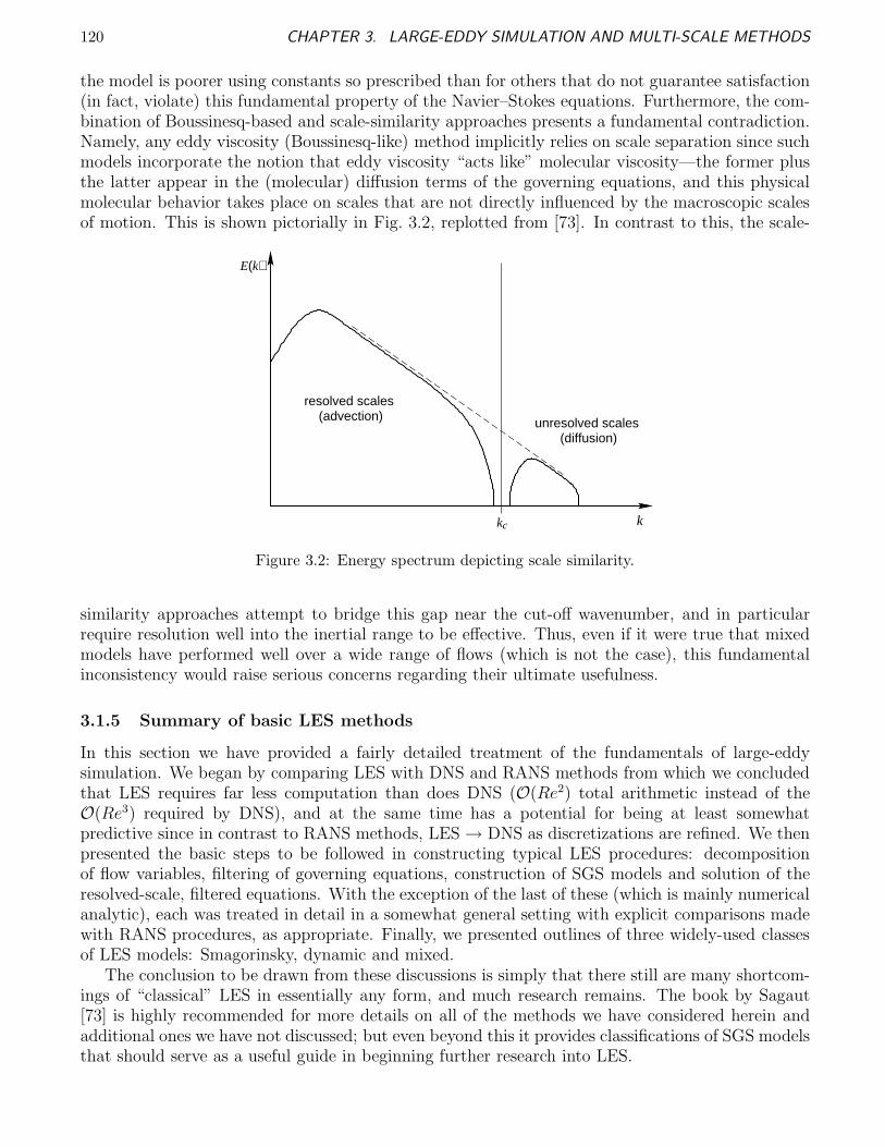
120 CHAPTER 3. LARGE-EDDY SIMULATION AND MULTI-SCALE METHODS
the model is poorer using constants so prescribed than for others that do not guarantee satisfaction(in fact, violate) this fundamental property of the Navier–Stokes equations. Furthermore, the com-bination of Boussinesq-based and scale-similarity approaches presents a fundamental contradiction.Namely, any eddy viscosity (Boussinesq-like) method implicitly relies on scale separation since suchmodels incorporate the notion that eddy viscosity “acts like” molecular viscosity—the former plusthe latter appear in the (molecular) diffusion terms of the governing equations, and this physicalmolecular behavior takes place on scales that are not directly influenced by the macroscopic scalesof motion. This is shown pictorially in Fig. 3.2, replotted from [73]. In contrast to this, the scale-
kc k
E(k)
resolved scales (advection) unresolved scales
(diffusion)
Figure 3.2: Energy spectrum depicting scale similarity.
similarity approaches attempt to bridge this gap near the cut-off wavenumber, and in particularrequire resolution well into the inertial range to be effective. Thus, even if it were true that mixedmodels have performed well over a wide range of flows (which is not the case), this fundamentalinconsistency would raise serious concerns regarding their ultimate usefulness.
3.1.5 Summary of basic LES methods
In this section we have provided a fairly detailed treatment of the fundamentals of large-eddysimulation. We began by comparing LES with DNS and RANS methods from which we concludedthat LES requires far less computation than does DNS (O(Re2) total arithmetic instead of theO(Re3) required by DNS), and at the same time has a potential for being at least somewhatpredictive since in contrast to RANS methods, LES → DNS as discretizations are refined. We thenpresented the basic steps to be followed in constructing typical LES procedures: decompositionof flow variables, filtering of governing equations, construction of SGS models and solution of theresolved-scale, filtered equations. With the exception of the last of these (which is mainly numericalanalytic), each was treated in detail in a somewhat general setting with explicit comparisons madewith RANS procedures, as appropriate. Finally, we presented outlines of three widely-used classesof LES models: Smagorinsky, dynamic and mixed.
The conclusion to be drawn from these discussions is simply that there still are many shortcom-ings of “classical” LES in essentially any form, and much research remains. The book by Sagaut[73] is highly recommended for more details on all of the methods we have considered herein andadditional ones we have not discussed; but even beyond this it provides classifications of SGS modelsthat should serve as a useful guide in beginning further research into LES.
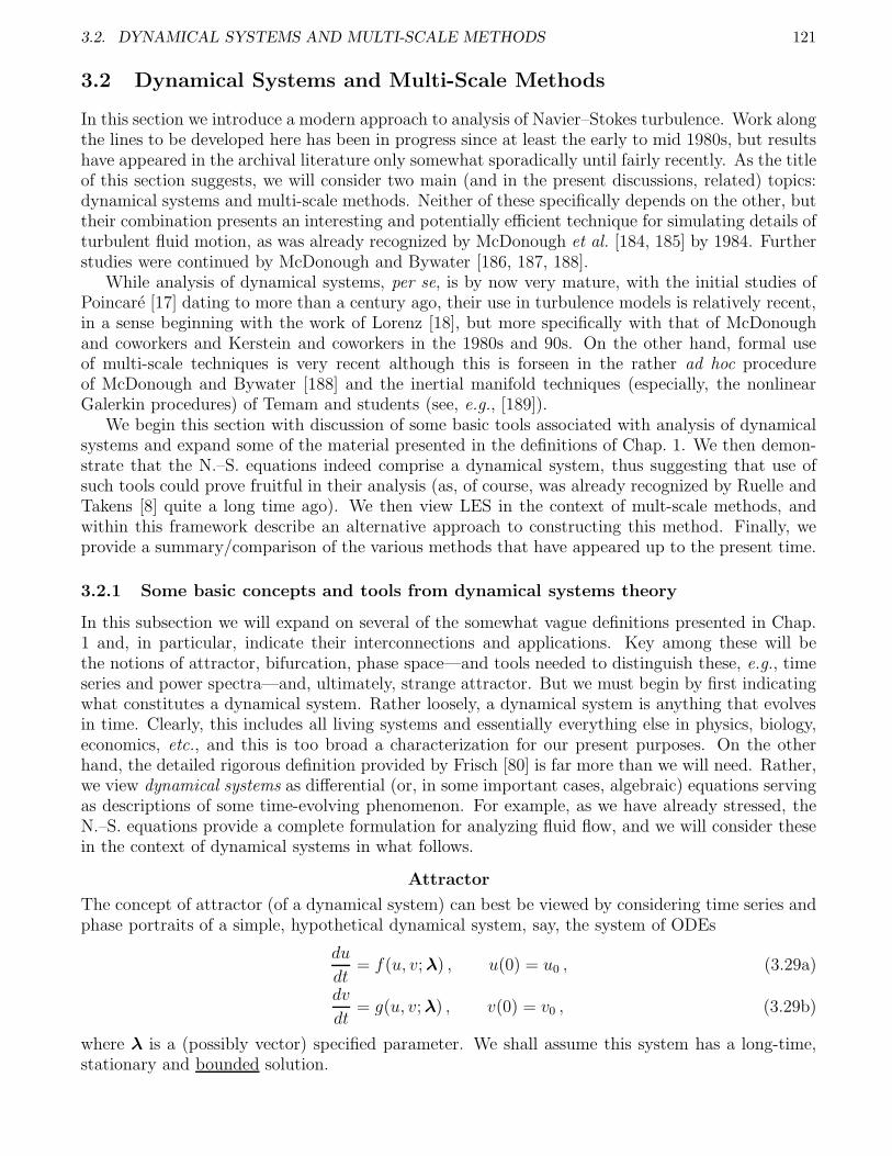
3.2. DYNAMICAL SYSTEMS AND MULTI-SCALE METHODS 121
3.2 Dynamical Systems and Multi-Scale Methods
In this section we introduce a modern approach to analysis of Navier–Stokes turbulence. Work alongthe lines to be developed here has been in progress since at least the early to mid 1980s, but resultshave appeared in the archival literature only somewhat sporadically until fairly recently. As the titleof this section suggests, we will consider two main (and in the present discussions, related) topics:dynamical systems and multi-scale methods. Neither of these specifically depends on the other, buttheir combination presents an interesting and potentially efficient technique for simulating details ofturbulent fluid motion, as was already recognized by McDonough et al. [184, 185] by 1984. Furtherstudies were continued by McDonough and Bywater [186, 187, 188].
While analysis of dynamical systems, per se, is by now very mature, with the initial studies ofPoincare [17] dating to more than a century ago, their use in turbulence models is relatively recent,in a sense beginning with the work of Lorenz [18], but more specifically with that of McDonoughand coworkers and Kerstein and coworkers in the 1980s and 90s. On the other hand, formal useof multi-scale techniques is very recent although this is forseen in the rather ad hoc procedureof McDonough and Bywater [188] and the inertial manifold techniques (especially, the nonlinearGalerkin procedures) of Temam and students (see, e.g., [189]).
We begin this section with discussion of some basic tools associated with analysis of dynamicalsystems and expand some of the material presented in the definitions of Chap. 1. We then demon-strate that the N.–S. equations indeed comprise a dynamical system, thus suggesting that use ofsuch tools could prove fruitful in their analysis (as, of course, was already recognized by Ruelle andTakens [8] quite a long time ago). We then view LES in the context of mult-scale methods, andwithin this framework describe an alternative approach to constructing this method. Finally, weprovide a summary/comparison of the various methods that have appeared up to the present time.
3.2.1 Some basic concepts and tools from dynamical systems theory
In this subsection we will expand on several of the somewhat vague definitions presented in Chap.1 and, in particular, indicate their interconnections and applications. Key among these will bethe notions of attractor, bifurcation, phase space—and tools needed to distinguish these, e.g., timeseries and power spectra—and, ultimately, strange attractor. But we must begin by first indicatingwhat constitutes a dynamical system. Rather loosely, a dynamical system is anything that evolvesin time. Clearly, this includes all living systems and essentially everything else in physics, biology,economics, etc., and this is too broad a characterization for our present purposes. On the otherhand, the detailed rigorous definition provided by Frisch [80] is far more than we will need. Rather,we view dynamical systems as differential (or, in some important cases, algebraic) equations servingas descriptions of some time-evolving phenomenon. For example, as we have already stressed, theN.–S. equations provide a complete formulation for analyzing fluid flow, and we will consider thesein the context of dynamical systems in what follows.
Attractor
The concept of attractor (of a dynamical system) can best be viewed by considering time series andphase portraits of a simple, hypothetical dynamical system, say, the system of ODEs
du
dt= f(u, v; λ) , u(0) = u0 , (3.29a)
dv
dt= g(u, v; λ) , v(0) = v0 , (3.29b)
where λ is a (possibly vector) specified parameter. We shall assume this system has a long-time,stationary and bounded solution.
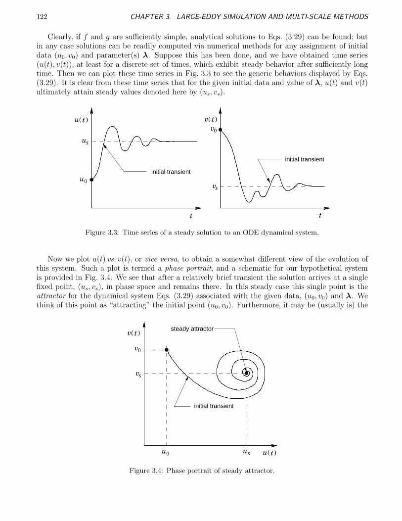
122 CHAPTER 3. LARGE-EDDY SIMULATION AND MULTI-SCALE METHODS
Clearly, if f and g are sufficiently simple, analytical solutions to Eqs. (3.29) can be found; butin any case solutions can be readily computed via numerical methods for any assignment of initialdata (u0, v0) and parameter(s) λ. Suppose this has been done, and we have obtained time series(u(t), v(t)), at least for a discrete set of times, which exhibit steady behavior after sufficiently longtime. Then we can plot these time series in Fig. 3.3 to see the generic behaviors displayed by Eqs.(3.29). It is clear from these time series that for the given initial data and value of λ, u(t) and v(t)ultimately attain steady values denoted here by (us, vs).
t( )v
0v
vs
t
initial transient
t( )u
us
u0
t
initial transient
Figure 3.3: Time series of a steady solution to an ODE dynamical system.
Now we plot u(t) vs. v(t), or vice versa, to obtain a somewhat different view of the evolution ofthis system. Such a plot is termed a phase portrait, and a schematic for our hypothetical systemis provided in Fig. 3.4. We see that after a relatively brief transient the solution arrives at a singlefixed point, (us, vs), in phase space and remains there. In this steady case this single point is theattractor for the dynamical system Eqs. (3.29) associated with the given data, (u0, v0) and λ. Wethink of this point as “attracting” the initial point (u0, v0). Furthermore, it may be (usually is) the
t( )v
0v
t( )u
vs
u0 us
steady attractor
initial transient
Figure 3.4: Phase portrait of steady attractor.
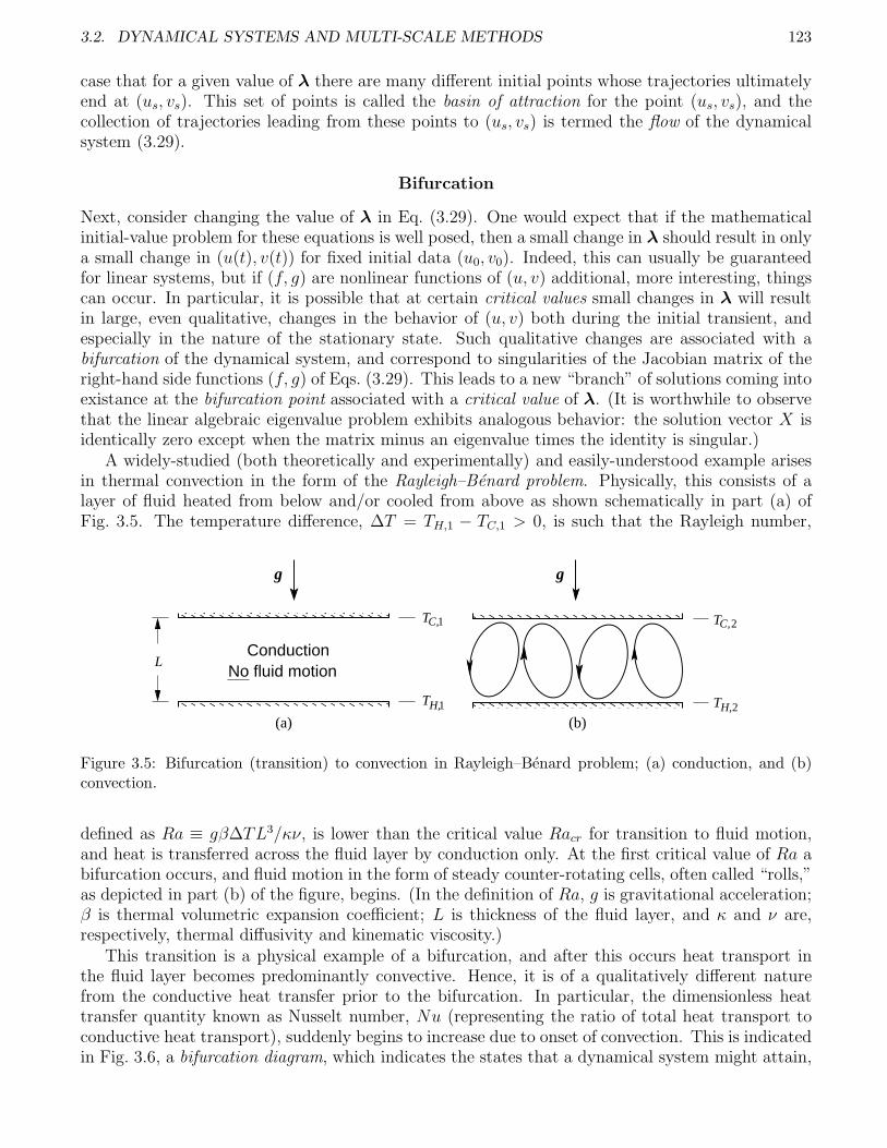
3.2. DYNAMICAL SYSTEMS AND MULTI-SCALE METHODS 123
case that for a given value of λ there are many different initial points whose trajectories ultimatelyend at (us, vs). This set of points is called the basin of attraction for the point (us, vs), and thecollection of trajectories leading from these points to (us, vs) is termed the flow of the dynamicalsystem (3.29).
Bifurcation
Next, consider changing the value of λ in Eq. (3.29). One would expect that if the mathematicalinitial-value problem for these equations is well posed, then a small change in λ should result in onlya small change in (u(t), v(t)) for fixed initial data (u0, v0). Indeed, this can usually be guaranteedfor linear systems, but if (f, g) are nonlinear functions of (u, v) additional, more interesting, thingscan occur. In particular, it is possible that at certain critical values small changes in λ will resultin large, even qualitative, changes in the behavior of (u, v) both during the initial transient, andespecially in the nature of the stationary state. Such qualitative changes are associated with abifurcation of the dynamical system, and correspond to singularities of the Jacobian matrix of theright-hand side functions (f, g) of Eqs. (3.29). This leads to a new “branch” of solutions coming intoexistance at the bifurcation point associated with a critical value of λ. (It is worthwhile to observethat the linear algebraic eigenvalue problem exhibits analogous behavior: the solution vector X isidentically zero except when the matrix minus an eigenvalue times the identity is singular.)
A widely-studied (both theoretically and experimentally) and easily-understood example arisesin thermal convection in the form of the Rayleigh–Benard problem. Physically, this consists of alayer of fluid heated from below and/or cooled from above as shown schematically in part (a) ofFig. 3.5. The temperature difference, ∆T = TH,1 − TC,1 > 0, is such that the Rayleigh number,
ConductionNo fluid motion
C,1T
H,1T
(a)
TC,2
TH,2
(b)
g g
L
Figure 3.5: Bifurcation (transition) to convection in Rayleigh–Benard problem; (a) conduction, and (b)convection.
defined as Ra ≡ gβ∆TL3/κν, is lower than the critical value Racr for transition to fluid motion,and heat is transferred across the fluid layer by conduction only. At the first critical value of Ra abifurcation occurs, and fluid motion in the form of steady counter-rotating cells, often called “rolls,”as depicted in part (b) of the figure, begins. (In the definition of Ra, g is gravitational acceleration;β is thermal volumetric expansion coefficient; L is thickness of the fluid layer, and κ and ν are,respectively, thermal diffusivity and kinematic viscosity.)
This transition is a physical example of a bifurcation, and after this occurs heat transport inthe fluid layer becomes predominantly convective. Hence, it is of a qualitatively different naturefrom the conductive heat transfer prior to the bifurcation. In particular, the dimensionless heattransfer quantity known as Nusselt number, Nu (representing the ratio of total heat transport toconductive heat transport), suddenly begins to increase due to onset of convection. This is indicatedin Fig. 3.6, a bifurcation diagram, which indicates the states that a dynamical system might attain,
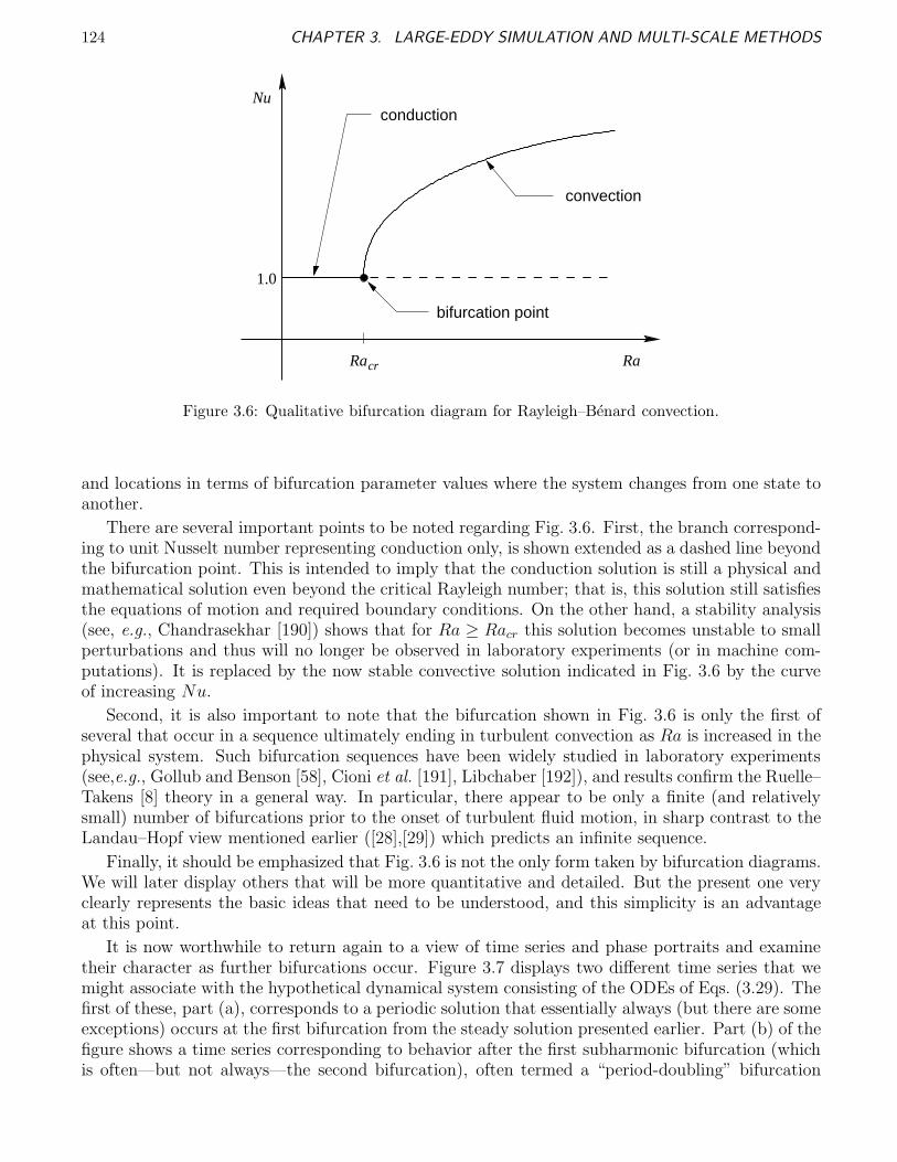
124 CHAPTER 3. LARGE-EDDY SIMULATION AND MULTI-SCALE METHODS
Racr
Nuconduction
convection
bifurcation point
1.0
Ra
Figure 3.6: Qualitative bifurcation diagram for Rayleigh–Benard convection.
and locations in terms of bifurcation parameter values where the system changes from one state toanother.
There are several important points to be noted regarding Fig. 3.6. First, the branch correspond-ing to unit Nusselt number representing conduction only, is shown extended as a dashed line beyondthe bifurcation point. This is intended to imply that the conduction solution is still a physical andmathematical solution even beyond the critical Rayleigh number; that is, this solution still satisfiesthe equations of motion and required boundary conditions. On the other hand, a stability analysis(see, e.g., Chandrasekhar [190]) shows that for Ra ≥ Racr this solution becomes unstable to smallperturbations and thus will no longer be observed in laboratory experiments (or in machine com-putations). It is replaced by the now stable convective solution indicated in Fig. 3.6 by the curveof increasing Nu.
Second, it is also important to note that the bifurcation shown in Fig. 3.6 is only the first ofseveral that occur in a sequence ultimately ending in turbulent convection as Ra is increased in thephysical system. Such bifurcation sequences have been widely studied in laboratory experiments(see,e.g., Gollub and Benson [58], Cioni et al. [191], Libchaber [192]), and results confirm the Ruelle–Takens [8] theory in a general way. In particular, there appear to be only a finite (and relativelysmall) number of bifurcations prior to the onset of turbulent fluid motion, in sharp contrast to theLandau–Hopf view mentioned earlier ([28],[29]) which predicts an infinite sequence.
Finally, it should be emphasized that Fig. 3.6 is not the only form taken by bifurcation diagrams.We will later display others that will be more quantitative and detailed. But the present one veryclearly represents the basic ideas that need to be understood, and this simplicity is an advantageat this point.
It is now worthwhile to return again to a view of time series and phase portraits and examinetheir character as further bifurcations occur. Figure 3.7 displays two different time series that wemight associate with the hypothetical dynamical system consisting of the ODEs of Eqs. (3.29). Thefirst of these, part (a), corresponds to a periodic solution that essentially always (but there are someexceptions) occurs at the first bifurcation from the steady solution presented earlier. Part (b) of thefigure shows a time series corresponding to behavior after the first subharmonic bifurcation (whichis often—but not always—the second bifurcation), often termed a “period-doubling” bifurcation
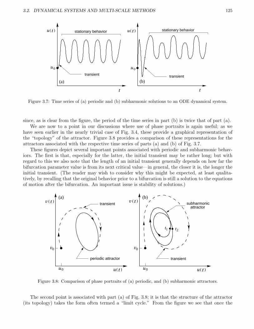
3.2. DYNAMICAL SYSTEMS AND MULTI-SCALE METHODS 125
t( )u
u0
(a)
transient
stationary behavior
t
t( )u
u0
(b)
stationary behavior
t
transient
Figure 3.7: Time series of (a) periodic and (b) subharmonic solutions to an ODE dynamical system.
since, as is clear from the figure, the period of the time series in part (b) is twice that of part (a).We are now to a point in our discussions where use of phase portraits is again useful; as we
have seen earlier in the nearly trivial case of Fig. 3.4, these provide a graphical representation ofthe “topology” of the attractor. Figure 3.8 provides a comparison of these representations for theattractors associated with the respective time series of parts (a) and (b) of Fig. 3.7.
These figures depict several important points associated with periodic and subharmonic behav-iors. The first is that, especially for the latter, the initial transient may be rather long; but withregard to this we also note that the length of an initial transient generally depends on how far thebifurcation parameter value is from its next critical value—in general, the closer it is, the longer theinitial transient. (The reader may wish to consider why this might be expected, at least qualita-tively, by recalling that the original behavior prior to a bifurcation is still a solution to the equationsof motion after the bifurcation. An important issue is stability of solutions.)
t( )u
t( )v
u0
v0
periodic attractor
transient
(a)t( )v
t( )u
v0
u0
t2t1
transient
attractorsubharmonic
(b)
Figure 3.8: Comparison of phase portraits of (a) periodic, and (b) subharmonic attractors.
The second point is associated with part (a) of Fig. 3.8; it is that the structure of the attractor(its topology) takes the form often termed a “limit cycle.” From the figure we see that once the
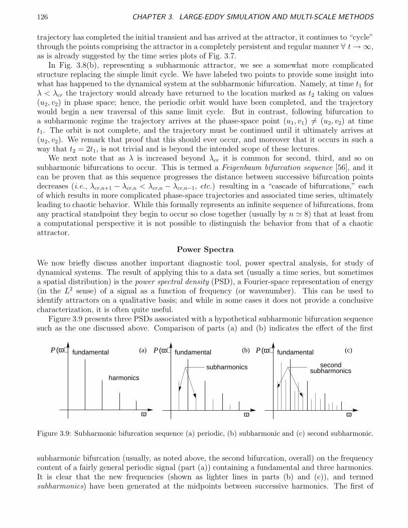
126 CHAPTER 3. LARGE-EDDY SIMULATION AND MULTI-SCALE METHODS
trajectory has completed the initial transient and has arrived at the attractor, it continues to “cycle”through the points comprising the attractor in a completely persistent and regular manner ∀ t → ∞,as is already suggested by the time series plots of Fig. 3.7.
In Fig. 3.8(b), representing a subharmonic attractor, we see a somewhat more complicatedstructure replacing the simple limit cycle. We have labeled two points to provide some insight intowhat has happened to the dynamical system at the subharmonic bifurcation. Namely, at time t1 forλ < λcr the trajectory would already have returned to the location marked as t2 taking on values(u2, v2) in phase space; hence, the periodic orbit would have been completed, and the trajectorywould begin a new traversal of this same limit cycle. But in contrast, following bifurcation toa subharmonic regime the trajectory arrives at the phase-space point (u1, v1) 6= (u2, v2) at timet1. The orbit is not complete, and the trajectory must be continued until it ultimately arrives at(u2, v2). We remark that proof that this should ever occur, and moreover that it occurs in such away that t2 = 2t1, is not trivial and is beyond the intended scope of these lectures.
We next note that as λ is increased beyond λcr it is common for second, third, and so onsubharmonic bifurcations to occur. This is termed a Feigenbaum bifurcation sequence [56], and itcan be proven that as this sequence progresses the distance between successive bifurcation pointsdecreases (i.e., λcr,n+1 − λcr,n < λcr,n − λcr,n−1, etc.) resulting in a “cascade of bifurcations,” eachof which results in more complicated phase-space trajectories and associated time series, ultimatelyleading to chaotic behavior. While this formally represents an infinite sequence of bifurcations, fromany practical standpoint they begin to occur so close together (usually by n ≃ 8) that at least froma computational perspective it is not possible to distinguish the behavior from that of a chaoticattractor.
Power Spectra
We now briefly discuss another important diagnostic tool, power spectral analysis, for study ofdynamical systems. The result of applying this to a data set (usually a time series, but sometimesa spatial distribution) is the power spectral density (PSD), a Fourier-space representation of energy(in the L2 sense) of a signal as a function of frequency (or wavenumber). This can be used toidentify attractors on a qualitative basis; and while in some cases it does not provide a conclusivecharacterization, it is often quite useful.
Figure 3.9 presents three PSDs associated with a hypothetical subharmonic bifurcation sequencesuch as the one discussed above. Comparison of parts (a) and (b) indicates the effect of the first
(ω)P
subharmonicssecond
(c)
ω
fundamental(ω)P
ω
(b)fundamental
subharmonics
(ω)P
ω
(a)fundamental
harmonics
Figure 3.9: Subharmonic bifurcation sequence (a) periodic, (b) subharmonic and (c) second subharmonic.
subharmonic bifurcation (usually, as noted above, the second bifurcation, overall) on the frequencycontent of a fairly general periodic signal (part (a)) containing a fundamental and three harmonics.It is clear that the new frequencies (shown as lighter lines in parts (b) and (c)), and termedsubharmonics) have been generated at the midpoints between successive harmonics. The first of
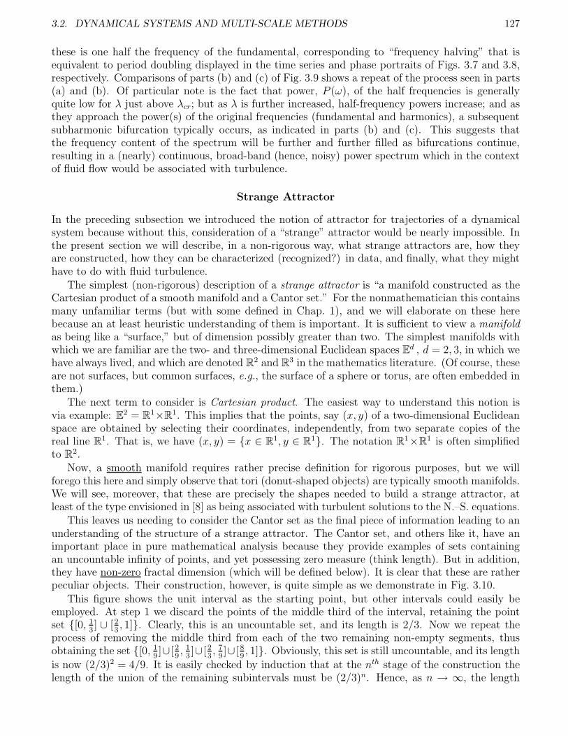
3.2. DYNAMICAL SYSTEMS AND MULTI-SCALE METHODS 127
these is one half the frequency of the fundamental, corresponding to “frequency halving” that isequivalent to period doubling displayed in the time series and phase portraits of Figs. 3.7 and 3.8,respectively. Comparisons of parts (b) and (c) of Fig. 3.9 shows a repeat of the process seen in parts(a) and (b). Of particular note is the fact that power, P (ω), of the half frequencies is generallyquite low for λ just above λcr; but as λ is further increased, half-frequency powers increase; and asthey approach the power(s) of the original frequencies (fundamental and harmonics), a subsequentsubharmonic bifurcation typically occurs, as indicated in parts (b) and (c). This suggests thatthe frequency content of the spectrum will be further and further filled as bifurcations continue,resulting in a (nearly) continuous, broad-band (hence, noisy) power spectrum which in the contextof fluid flow would be associated with turbulence.
Strange Attractor
In the preceding subsection we introduced the notion of attractor for trajectories of a dynamicalsystem because without this, consideration of a “strange” attractor would be nearly impossible. Inthe present section we will describe, in a non-rigorous way, what strange attractors are, how theyare constructed, how they can be characterized (recognized?) in data, and finally, what they mighthave to do with fluid turbulence.
The simplest (non-rigorous) description of a strange attractor is “a manifold constructed as theCartesian product of a smooth manifold and a Cantor set.” For the nonmathematician this containsmany unfamiliar terms (but with some defined in Chap. 1), and we will elaborate on these herebecause an at least heuristic understanding of them is important. It is sufficient to view a manifoldas being like a “surface,” but of dimension possibly greater than two. The simplest manifolds withwhich we are familiar are the two- and three-dimensional Euclidean spaces Ed , d = 2, 3, in which wehave always lived, and which are denoted R2 and R3 in the mathematics literature. (Of course, theseare not surfaces, but common surfaces, e.g., the surface of a sphere or torus, are often embedded inthem.)
The next term to consider is Cartesian product. The easiest way to understand this notion isvia example: E2 = R1×R1. This implies that the points, say (x, y) of a two-dimensional Euclideanspace are obtained by selecting their coordinates, independently, from two separate copies of thereal line R1. That is, we have (x, y) = x ∈ R1, y ∈ R1. The notation R1×R1 is often simplifiedto R2.
Now, a smooth manifold requires rather precise definition for rigorous purposes, but we willforego this here and simply observe that tori (donut-shaped objects) are typically smooth manifolds.We will see, moreover, that these are precisely the shapes needed to build a strange attractor, atleast of the type envisioned in [8] as being associated with turbulent solutions to the N.–S. equations.
This leaves us needing to consider the Cantor set as the final piece of information leading to anunderstanding of the structure of a strange attractor. The Cantor set, and others like it, have animportant place in pure mathematical analysis because they provide examples of sets containingan uncountable infinity of points, and yet possessing zero measure (think length). But in addition,they have non-zero fractal dimension (which will be defined below). It is clear that these are ratherpeculiar objects. Their construction, however, is quite simple as we demonstrate in Fig. 3.10.
This figure shows the unit interval as the starting point, but other intervals could easily beemployed. At step 1 we discard the points of the middle third of the interval, retaining the pointset [0, 1
3] ∪ [2
3, 1]. Clearly, this is an uncountable set, and its length is 2/3. Now we repeat the
process of removing the middle third from each of the two remaining non-empty segments, thusobtaining the set [0, 1
9]∪ [2
9, 1
3]∪ [2
3, 7
9]∪ [8
9, 1]. Obviously, this set is still uncountable, and its length
is now (2/3)2 = 4/9. It is easily checked by induction that at the nth stage of the construction thelength of the union of the remaining subintervals must be (2/3)n. Hence, as n → ∞, the length
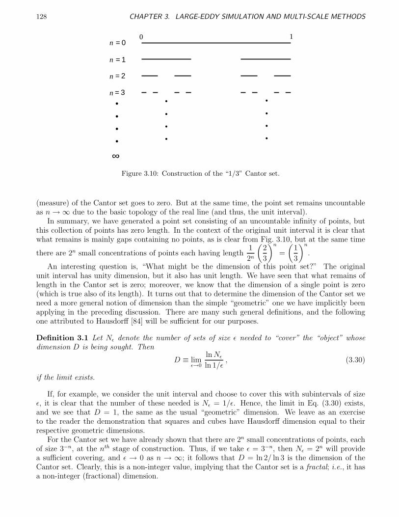
128 CHAPTER 3. LARGE-EDDY SIMULATION AND MULTI-SCALE METHODS
= 0n
= 1n
= 2n
= 3n
.
.
.
....
.....
0 1
Figure 3.10: Construction of the “1/3” Cantor set.
(measure) of the Cantor set goes to zero. But at the same time, the point set remains uncountableas n → ∞ due to the basic topology of the real line (and thus, the unit interval).
In summary, we have generated a point set consisting of an uncountable infinity of points, butthis collection of points has zero length. In the context of the original unit interval it is clear thatwhat remains is mainly gaps containing no points, as is clear from Fig. 3.10, but at the same time
there are 2n small concentrations of points each having length1
2n
(2
3
)n
=
(1
3
)n
.
An interesting question is, “What might be the dimension of this point set?” The originalunit interval has unity dimension, but it also has unit length. We have seen that what remains oflength in the Cantor set is zero; moreover, we know that the dimension of a single point is zero(which is true also of its length). It turns out that to determine the dimension of the Cantor set weneed a more general notion of dimension than the simple “geometric” one we have implicitly beenapplying in the preceding discussion. There are many such general definitions, and the followingone attributed to Hausdorff [84] will be sufficient for our purposes.
Definition 3.1 Let Nǫ denote the number of sets of size ǫ needed to “cover” the “object” whosedimension D is being sought. Then
D ≡ limǫ→0
ln Nǫ
ln 1/ǫ, (3.30)
if the limit exists.
If, for example, we consider the unit interval and choose to cover this with subintervals of sizeǫ, it is clear that the number of these needed is Nǫ = 1/ǫ. Hence, the limit in Eq. (3.30) exists,and we see that D = 1, the same as the usual “geometric” dimension. We leave as an exerciseto the reader the demonstration that squares and cubes have Hausdorff dimension equal to theirrespective geometric dimensions.
For the Cantor set we have already shown that there are 2n small concentrations of points, eachof size 3−n, at the nth stage of construction. Thus, if we take ǫ = 3−n, then Nǫ = 2n will providea sufficient covering, and ǫ → 0 as n → ∞; it follows that D = ln 2/ ln 3 is the dimension of theCantor set. Clearly, this is a non-integer value, implying that the Cantor set is a fractal; i.e., it hasa non-integer (fractional) dimension.
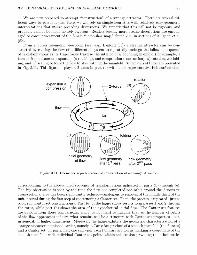
3.2. DYNAMICAL SYSTEMS AND MULTI-SCALE METHODS 129
We are now prepared to attempt “construction” of a strange attractor. There are several dif-ferent ways to go about this. Here, we will rely on simple heuristics with relatively easy geometricinterpretations that utilize preceding discussions. We remark that this will not be rigorous, andprobably cannot be made entirely rigorous. Readers seeking more precise descriptions are encour-aged to consult treatment of the Smale “horse-shoe map,” found e.g., in sections of Alligood et al.[85].
From a purely geometric viewpoint (see, e.g., Lanford [86]) a strange attractor can be con-structed by causing the flow of a differential system to repeatedly undergo the following sequenceof transformations as its trajectories traverse the interior of a bounding manifold (for example, atorus): i) simultaneous expansion (stretching), and compression (contraction), ii) rotation, iii) fold-ing, and iv) scaling to force the flow to stay withing the manifold. Schematics of these are presentedin Fig. 3.11. This figure displays a 2-torus in part (a) with some representative Poincare sections
compressionexpansion &
after 1 passstflow geometry
after 2nd passflow geometry
2−torus
flow
initial geometryof flow
rotation
(a)
(d)
(e)(b)
(c)
folding
Figure 3.11: Geometric representation of construction of a strange attractor.
corresponding to the above-noted sequence of transformations indicated in parts (b) through (e).The key observation is that by the time the flow has completed one orbit around the 2-torus itscross-sectional area has been significantly reduced—analogous to removal of the middle third of theunit interval during the first step of constructing a Cantor set. Then, the process is repeated (just asoccurs in Cantor set constructions). Part (e) of the figure shows results from passes 1 and 2 throughthe torus, while part (b) shows the area of the hypothetical initial flow. The Cantor set featuresare obvious from these comparisons, and it is not hard to imagine that as the number of orbitsof the flow approaches infinity, what remains will be a structure with Cantor set properties—but,in general, in higher dimensions. Moreover, the figure exhibits the geometric characterization of astrange attractor mentioned earlier, namely, a Cartesian product of a smooth manifold (the 2-torus)and a Cantor set. In particular, one can view each Poincare section as marking a coordinate of thesmooth manifold, with individual Cantor set points within this section providing the other entries

130 CHAPTER 3. LARGE-EDDY SIMULATION AND MULTI-SCALE METHODS
of the Cartesian product.There are a couple important items to consider with regard to this construction. First, for
continuous dynamical systems these heuristics suggest that dimension three (in phase space) is thesmallest system that can produce a strange attractor. Moreover, the fractal dimension of any suchattractor is greater than two. We remark that these are provable statements (see, e.g., [77]).
The next point to consider is what is required in a dynamical system to permit it to carry outthe required transformations. There are two key properties. The first is nonlinearity. If we recallthe Galerkin representation of the N.–S. equations of Chap. 1 where we noted that the nonlinearterms are capable of generating modes that were not present in prescribed initial data, we seethat there is an intrinsic capacity to generate complicated phase-space behaviors associated withstretching and rotation. The second property required to create a strange attractor is dissipation.Especially the expansive behaviors of the nonlinear terms must be controlled in order to producean attractor; and as was emphasized in our Galerkin procedure analyses of the N.–S. equations,this is accomplished with dissipation. In particular, in the phase-space context we can also viewdissipation as producing contraction of the flow, and scaling in general, to allow it to remain withina bounding mainfold. But in addition, it is reasonable to consider the combination of nonlinearityand dissipation as contributing to the folding process. In summary, we observe that in order fora continuous dynamical system to be able to generate a strange attractor, it must be of at leastdimension three in phase space; it must be nonlinear, and it must be dissipative.
We remark that by way of contrast, for a discrete dynamical system (algebraic map), threedimensionality is not required (but, of course, is permitted) for existence of a strange attractor.Indeed, simple 1-D quadratic maps such as the logistic map
x(m+1) = βx(m)(1 − x(m)
), 0 < β ≤ 4 , (3.31)
studied by May [193] exhibit the chaotic temporal behavior of a strange attractor. Moreover, a2-D discrete map due to Henon exhibits another property often associated with strange attractors,namely scale similarity. This can be seen in the Cantor set of Fig. 3.10; in particular, one sees thatif construction were started at the first step rather than at the zeroth one, the results would be thesame up to a rescaling of lengths, as hinted earlier; clearly, this is true ∀ n<∞. The Henon mapis generated from the algebraic system
x(m+1) = 1 − ax(m) 2 + y(m) , (3.32a)
y(m+1) = bx(m) , (3.32b)
usually computed using a = 1.4 and b = 0.3. This is presented by Henon [194] as a Poincare map ofthe Lorenz equations [18], although this is in the framework of an argument and construction thatis not especially rigorous. Figure 3.12, a phase portrait for this discrete dynamical system (DDS)(3.32), displays the scale similarity property.
We observe that as we continue to focus on finer and finer scales we see repetition of the basicstructure. This is evidence of the Cantor set-like construction, now for a concrete example. Inparticular, part (a) of Fig. 3.12 displays the usual phase portrait of the Henon attractor generatedfrom Eqs. (3.32) starting with initial data x0 = y0 = 0. This figure at first appears rather unre-markable, consisting of a few seemingly smooth curves. Moreover, a first zoom-in in a neighborhoodof [−0.1, 0.1]×[0.2, 0.3], part (b) of the figure, seems to confirm this. But a further finer-scale regioninterior to [−0.002, 0.002]×[0.268, 0.272] shown in part (c) indicates significant structure. Here wesee a sequence of bands of points arranged successively (from bottom to top) in groups consistingof a single band, two bands, and then three bands. (We remark that these bands are clearly notcontinuous curves; they contain many gaps just as do the later steps of the Cantor set.)
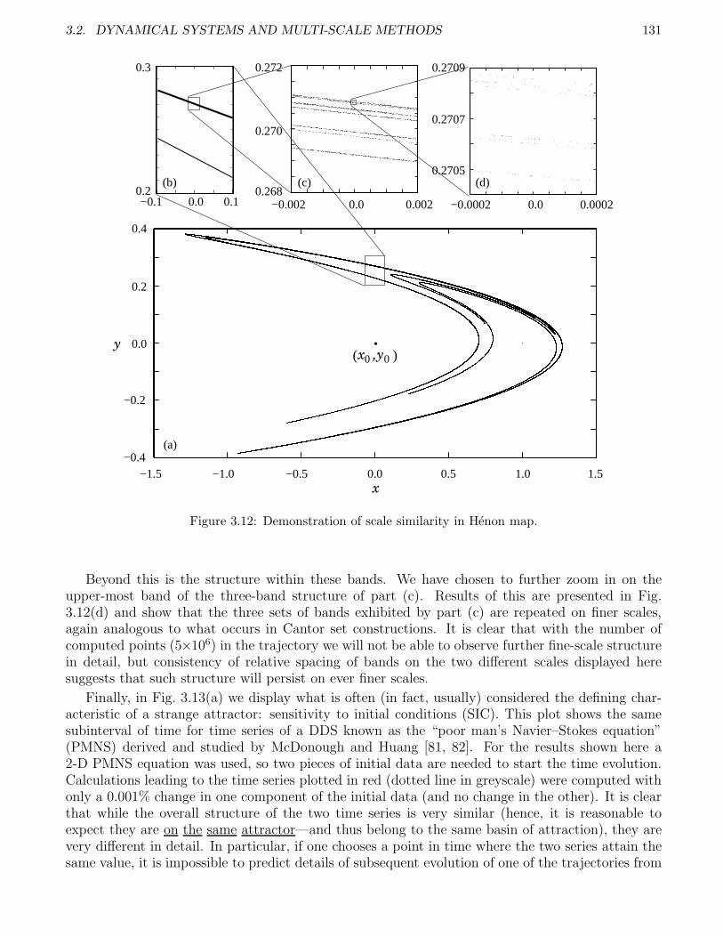
3.2. DYNAMICAL SYSTEMS AND MULTI-SCALE METHODS 131
0.10.0−0.1
0.3
0.20.0002−0.0002 0.0
0.2705
0.2707
0.2709
0.270
0.272
0.2680.0020.0−0.002
−0.5 0.0 0.5 1.0 1.5−1.5 −1.0
0.4
0.2
−0.4
−0.2
0.0y
x
.x ,y0 0( )
(c) (d)(b)
(a)
Figure 3.12: Demonstration of scale similarity in Henon map.
Beyond this is the structure within these bands. We have chosen to further zoom in on theupper-most band of the three-band structure of part (c). Results of this are presented in Fig.3.12(d) and show that the three sets of bands exhibited by part (c) are repeated on finer scales,again analogous to what occurs in Cantor set constructions. It is clear that with the number ofcomputed points (5×10⁶) in the trajectory we will not be able to observe further fine-scale structurein detail, but consistency of relative spacing of bands on the two different scales displayed heresuggests that such structure will persist on ever finer scales.
Finally, in Fig. 3.13(a) we display what is often (in fact, usually) considered the defining char-acteristic of a strange attractor: sensitivity to initial conditions (SIC). This plot shows the samesubinterval of time for time series of a DDS known as the “poor man’s Navier–Stokes equation”(PMNS) derived and studied by McDonough and Huang [81, 82]. For the results shown here a2-D PMNS equation was used, so two pieces of initial data are needed to start the time evolution.Calculations leading to the time series plotted in red (dotted line in greyscale) were computed withonly a 0.001% change in one component of the initial data (and no change in the other). It is clearthat while the overall structure of the two time series is very similar (hence, it is reasonable toexpect they are on the same attractor—and thus belong to the same basin of attraction), they arevery different in detail. In particular, if one chooses a point in time where the two series attain thesame value, it is impossible to predict details of subsequent evolution of one of the trajectories from
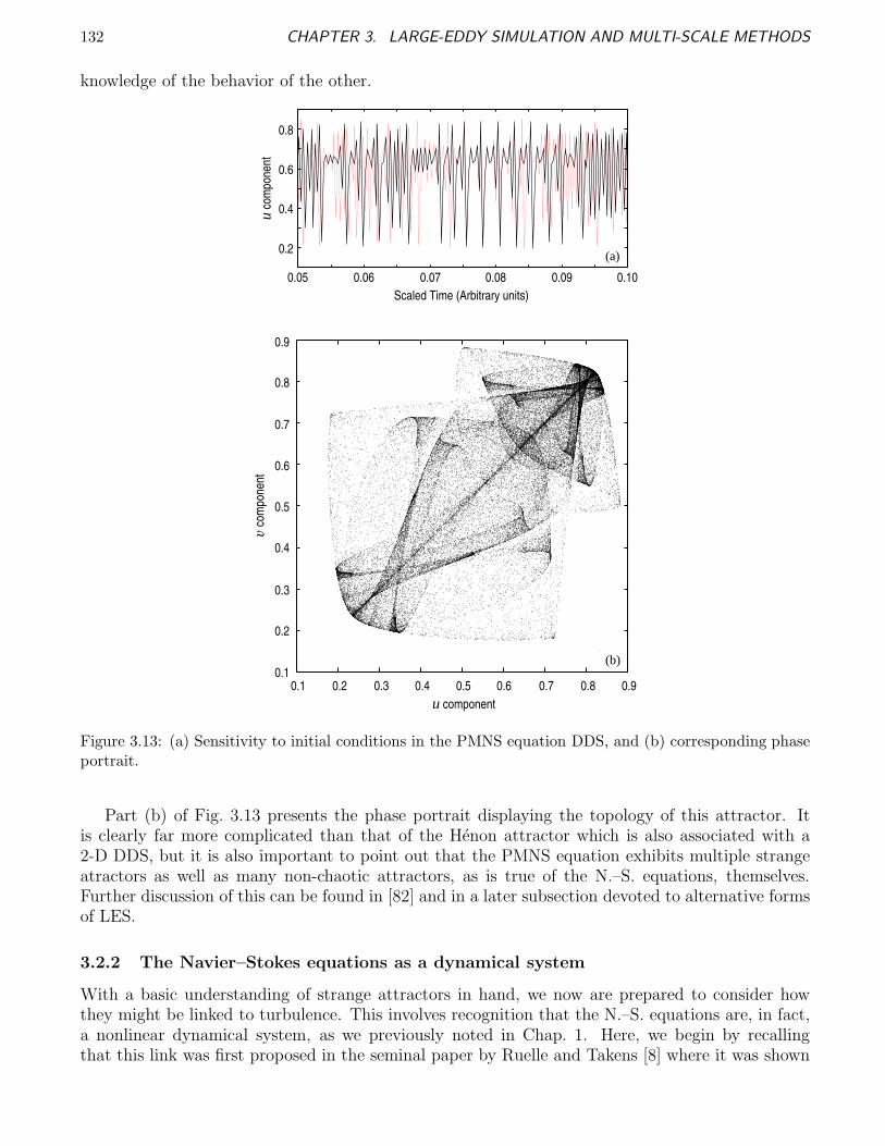
132 CHAPTER 3. LARGE-EDDY SIMULATION AND MULTI-SCALE METHODS
knowledge of the behavior of the other.
0.1
0.2
0.3
0.4
0.5
0.6
0.7
0.8
0.9
14.05 14.055 14.06 14.065 14.07 14.075 14.08 14.085 14.09 14.095 14.10.1
0.2
0.3
0.4
0.5
0.6
0.7
0.8
0.9
14.05 14.055 14.06 14.065 14.07 14.075 14.08 14.085 14.09 14.095 14.1
Scaled Time (Arbitrary units)
u co
mpo
nent
0.2
0.4
0.8
0.6
0.05 0.06 0.07 0.08 0.09 0.10
(a)
0.1
0.2
0.3
0.4
0.5
0.6
0.7
0.8
0.9
0.1 0.2 0.3 0.4 0.5 0.6 0.7 0.8 0.90.1
0.2
0.3
0.4
0.5
0.6
0.7
0.8
0.9
0.1 0.2 0.3 0.4 0.5 0.6 0.7 0.8 0.9
u component
v c
ompo
nent
(b)
(a)
(b)
Figure 3.13: (a) Sensitivity to initial conditions in the PMNS equation DDS, and (b) corresponding phaseportrait.
Part (b) of Fig. 3.13 presents the phase portrait displaying the topology of this attractor. Itis clearly far more complicated than that of the Henon attractor which is also associated with a2-D DDS, but it is also important to point out that the PMNS equation exhibits multiple strangeatractors as well as many non-chaotic attractors, as is true of the N.–S. equations, themselves.Further discussion of this can be found in [82] and in a later subsection devoted to alternative formsof LES.
3.2.2 The Navier–Stokes equations as a dynamical system
With a basic understanding of strange attractors in hand, we now are prepared to consider howthey might be linked to turbulence. This involves recognition that the N.–S. equations are, in fact,a nonlinear dynamical system, as we previously noted in Chap. 1. Here, we begin by recallingthat this link was first proposed in the seminal paper by Ruelle and Takens [8] where it was shown
3.2. DYNAMICAL SYSTEMS AND MULTI-SCALE METHODS 133
that phase-space trajectories corresponding to a flow of the N.–S. equations (viewed as a dynamicalsystem) become attracted to a topological object having properties we have just discussed. Theytermed this a “strange attractor,” and proposed that its temporally chaotic behavior should beassociated with physical turbulence. It is interesting to also note that Lorenz [18] had earliercomputed similar trajectories for a severely truncated Galerkin approximation of the N.–S. andthermal energy equations (also a dynamical system) and used sensitivity to initial conditions ofsolutions to these equations to conclude that long-range weather prediction would never be possible.We should observe, however, that while the equations due to Lorenz do exhibit a strange attractorin their solutions for certain ranges of parameter values, the bifurcation sequence leading to suchstates is different from that studied in [8].
But beyond the fact, already used in [8], that the N.–S. equations comprise a dynamical systemis the experimental observation that typically only short bifurcation sequences occur before flowbehaviors are chaotic and sensitive to initial conditions, and thus associated with physical turbu-lence. In particular, experiments with fluid flow (and other physical phenomena) have identified atleast three distinct short bifurcation sequences leading to physical chaos, and they have also beenobserved and studied analytically and computationally. These are the following (characterized byqualitative system description of the various states):
steady −→ periodic −→ subharmonic −→ chaotic ,
steady −→ periodic −→ quasiperiodic −→ chaotic ,
steady −→ periodic −→ intermittent −→ chaotic .
The first of these was studied by Feigenbaum [56] in the context of the simple algebraic map, Eq.(3.31), first studied by May [193], as noted earlier. But numerical solutions to the N.–S. equationsalso exhibit such a sequence in the context of boundary layer transition, as reported by Pulliam andVastano [195]. The second sequence is that originally proposed by Ruelle and Takens [8], and which,as noted earlier, has been observed (with some modification) in numerous laboratory experiments(e.g., those of Gollub and Benson [58]) and simulations. The final sequence given here was firststudied by Pomeau and Manneville [57] (see also [77]). We remark that in these works, and infurther studies cited therein, the authors identified three distinct types of intermittency, all of whichhave been observed in physical experiments but not yet conclusively in N.–S. equation simulations(possibly because they tend to occur at values of Re well above those currently accessible via DNS).Finally, we observe that various combinations of these sequences have been seen in both experimentsand computations, but in all cases the route to chaos consists of relatively few bifurcations.
Thus, both computations with the N.–S. equations and laboratory investigations of physicalfluid flows generally support the Ruelle and Takens view and contradict predictions of the Landau–Hopf theory which proposed that turbulence was the result of an infinite sequence of quasiperiodicbifurcations, each of which produced an additional incommensurate frequency. While any suchflow could be very complicated, as would be its power spectrum, it would lack SIC and the fractaldimension seen in modern laboratory experiments and DNS of the N.–S. equations.
While the preceding discussions appear to support the chaotic dynamics/strange attractor viewof turbulence, there are two main arguments often given against this interpretation. The first ofthese is the claim that dynamical systems produce only temporal chaos while it is well knownthat turbulence exhibits both temporal and spatial chaotic behavior. Here, we propose that thisargument is completely fallacious, arising from a lack of understanding of the N.–S. equations andthe (mathematical) nature of their solution structure. In particular, it ignores the fact that Fourierrepresentations with temporally chaotic coefficients will automatically produce spatial chaos as aconsequence of different linear combinations of these coefficients (via different values taken on by
134 CHAPTER 3. LARGE-EDDY SIMULATION AND MULTI-SCALE METHODS
basis functions) at each spatial location and effects arising from SIC associated with spatially-distributed initial data. This is clearly observed in DNS, and even in well-resolved LES. Thoseadherring to claim of no connection between dynamical systems and turbulence must forego useof (DNS of) the N.–S. equations for their argument to self consistent—and very few researchersin the modern era would be willing to do this (fortunately) after all the success experienced withsimuation via these equations.
The second criticism of the “strange attractor theory of turbulence” is more serious—especiallyfrom a practical, computational viewpoint. It is that, to date, the theory of dynamical systems(aside from use of DNS) has failed to produce any computational tools for practical simulations ofturbulence. Although there have been scattered exceptions to this (for example, the shell modelsdescribed in Bohr et al. [83]), they have for the most part represented rather anecdotal results, asopposed to well-founded, general formulations capable of wide application. We note that the one-dimensional turbulence (ODT) model of Kerstein and coworkers (see, e.g., Echekki et al. )[71]), anoutgrowth of Kerstein’s linear-eddy models (LEMs), is to some extent proving to provide fairly wideapplicability. In addition, we will in the next subsection provide details of a new modeling approachthat appears to hold significant promise, primarily because of its firm foundations in theory of theN.–S. equations.
3.2.3 Multi-scale methods and alternative approaches to LES
In this subsection we will treat two main, related, topics: i) the basics of multi-scale methods, andii) application of these techniques to an alternative formulation for LES. The first of these is acurrent topic of accelerating research in numerical analysis, and complete journals are now devotedto this area. The second is not new; but in the past, work has been sporadic and not necessarily wellfounded on a mathematical basis. Here, we will attempt to remedy this by providing a differentapproach to constructing LES procedures in considerable detail and justifying this with formalmathematics—but in the absence of rigorous proofs. As part of this, we will supply a pseudo-language algorithm presenting an outline of the steps needed to produce a computational LES codebased on this approach.
Basics of Multi-Scale Methods
The goal of multi-scale formalisms, in general, is to provide computationally-efficient techniques forsolving problems possessing a wide range of space and/or time scales. The need to do this has beenrecognized from the beginning of turbulence simulation, but in recent years it has been identified inmany other areas (e.g., laminar flow in porous media and solidification of crystals in liquid melts)giving rise to attempts to construct a general theory applicable across a broad spectrum of problemtypes (physical situations) and at the same time able to be analyzed by formal mathematicaltechniques. In the present section we provide a qualitative discussion of such methods.
To begin we should make clear precisely why computing over a wide range of scales is a “problem”in order to motivate approaches now being employed in constructing multi-scale methods. As wehave already discussed, specifically in the context of turbulent fluid flow, if a complete solutionis to be computed it is necessary to resolve all physically-relevant scales—DNS in this context.Moreover, as we have also already emphasized, the range of scales can be very large. For example,in considering prediction of lift or drag for an aircraft, the structure of turbulent ambient air containsscales ranging from at least tens of kilometers down to millimeters, and the flow containing thesescales interacts with the surface of the aircraft on scales of tens of meters down to smaller thanmillimeters. Hence, there are seven to eight orders of magnitude in the range of spatial scales neededto accurately predict lift and drag on an aircraft flying through a cumulous cloud. This is presentlynot a tractable calculation, and various approximations must be made—which, of course, motivates
3.2. DYNAMICAL SYSTEMS AND MULTI-SCALE METHODS 135
the need for computational procedures much more efficient than DNS but at the same time able tocapture much of the physics currently only accessible via DNS.
But this represents only the beginnings of the difficulties. If, for example, heat transfer and/orchemistry are important parts of the physics then, especially in the latter case, far smaller spatialscales are needed; and relevant time scales can span a range of minutes down to elementary reactiontimes of 10−8 seconds, or less. Furthermore, it is now the case that different physics, requiring diversemathematical representations, may occur in different ranges of scales. For example, at nanoscalesthe continuum hypothesis is no longer valid, and the N.–S. equations must be replaced with theBoltzmann equation.
It is clear in all such cases that a brute-force use of direct simulation will probably not befeasible for many years—some would argue, never—without radical changes in computing hardwarearchitectures, and yet analysis of such problems is becoming increasingly important. The multi-scaleformalisms now being developed represent attempts to address this issue.
There are several key ideas that are combined to produce multi-scale algorithms, in general.But not all such algorithms contain all of these, at least not explicitly. The first is to identifythe important scales needed to sufficiently represent the problem and attempt to obtain equationsrepresenting the physics on each of these. In some cases, as noted by E and Engquist [131, 196],these equations may not be known; then one of the goals of a multi-scale formalism is to bypass theneed for such unknown equations. This will not be the case for our specific purposes herein, andwe will have little more to say regarding this aspect of multi-scale procedures.
After identifying the scales (and their appropriate mathematical representations), it is thennecessary to construct efficient solution procedures on (for) each of these. As we will see, it is notusually efficient to employ the same type of algorithm on all scales; moreover, it is typical to resortto more approximation as inherent arithmetic complexity increases. In particular, models employedon the smallest scales where high resolution is most difficult are often the most approximate. Butwe remark that this can often be reasonably-well justified with both physical and mathematicalarguments.
From an algorithmic standpoint, the final aspect to consider in a multi-scale formalism is com-bining results from the various represented scales to obtain a complete solution. In [196] it ispointed out that this is a highly nontrivial mathematical problem, and much research regardingthis is in progress. Furthermore, we remark that there are numerous ways (some of them ratherobvious) in which this can be done, but it must be emphasized, as done in [196], that essentiallyany procedure brings with it questions associated with stability and consistency of the overall (nu-merical) procedure. Thus, the final aspect of any multi-scale method is its mathematical analysis;it is important to be able to prove that solutions obtained from a multi-scale algorithm converge tothose that would be obtained from a highly-accurate (fully-resolved) approach if this is appropriate.Of course, as already hinted, this is not always the case. We will not herein devote much space tosuch analyses despite their importance, as they are the subjects of current research, and instead werefer the reader to the cited literature.
Probably the oldest examples of multi-scale approaches are the homogenization and renormaliza-tion group (RNG) techniques. Aspects of these methods have motivated some of the formal analysisof modern multi-scale procedures. Moreover, as we will consider in more detail below, at least SGSmodels for LES, but possibly even RANS models, might be viewed as forms of homogenization—and some have been derived via RNG (see, e.g., [93]). The basic idea in any such approach is toalter physical transport properties to enable taking into account physics on scales that have notbeen explicitly resolved by the discretization employed for the numerical solution process. That is,homogenization provides a modeling technique that accounts for the effects of small-scale physicswithout actually representing that physics in detail, as is also true of RNG models. Recall thatthis is precisely what takes place in both RANS and LES SGS models. At the same time it

136 CHAPTER 3. LARGE-EDDY SIMULATION AND MULTI-SCALE METHODS
must be recognized that there are formal mathematical requirements and techniques associatedwith homogenization—see Marchenko and Khuslov [197] (and RNG approaches), and these are notgenerally followed during construction of RANS and SGS models.
In the present discussions we will not specifically emphasize homogenization aspects of multi-scale methods but instead provide some basic heuristics. We begin with Fig. 3.14 which depicts aportion of a coarse-resolution grid on which regions of high resolution have been indicated. This
hx
hy
Figure 3.14: Example multi-scale gridding.
type of discrete structuring would be appropriate in situations for which the coarse-grid resolutionis globally inadequate, but in which the indicated local resolution could not be supported globally.In principle, multi-scale formalisms provide techniques by means of which relatively inexpensivelocal fine-grid calculations can be combined with the also relatively inexpensive global coarse-gridresults.
In particular, in the context of the grid displayed in Fig. 3.14, the high-resolution portion, asshown, covers only about one third of the complete domain area, so even if the fine-grid calculationswere completely coupled, total arithmetic would be no more than about one-nineth that requiredon a complete high-resolution grid (in 2D—and relatively less in 3D). But these subdomains are notdirectly coupled. Hence, total arithmetic is further reduced, and, beyond this, the decoupling ofsubdomains provides an opportunity for parallelization to further improve computational efficiency.
It is clear that if the coarse- and fine-grid results can be combined correctly, it should be possibleto improve the coarse-grid solution. The basic question is “How should this be done?” Here, we willdiscuss some possible alternatives. One can envision at least two main classes of approaches to thisproblem. First, one could perform local calculations on the small, highly-resolved subdomains andcompare computed results at the embedded large-scale grid points to estimate required modificationsto large-scale transport property values. This might be viewed as a form of homogenization. Asecond possibility is more closely related to function decompositions employed in LES (and in

3.2. DYNAMICAL SYSTEMS AND MULTI-SCALE METHODS 137
RANS) and involves using fine-grid local calculations to directly enhance coarse-grid results. Ineither approach, calculations on the subdomains must be performed, and it is mainly the manner inwhich these are used that distinguishes the two techniques. We remark that mathematical analysisof these approaches is, for the most part, still lacking.
Thus, we begin with a description of these calculations. Because, as they are presented inFig. 3.14, the small-scale subdomains are completely disjoint, and as a consequence the small-scalesolution in one subdomain cannot “know” anything about the corresponding solutions in any neigh-boring domain. In physical situations dominated by diffusion one might argue that if the large-scaletime step is less than the diffusion time between coarse-grid points, then this lack of communicationis not a serious concern—at least if effects of this are somehow included in the coarse-grid calcu-lations, e.g., via alteration of transport properties (as in RNG or homogenization methods). Butif the physics of the problem under consideration is not diffusion dominated, calculations based oncompletely separated high-resolution small-scale domains will probably be inaccurate, and possiblycompletely incorrect. Hence, a general approach should attempt to provide some communicationbetween neighboring small-scale subdomains.
We can envision at least two specific situations, each arising from a different representationof the overall solution associated with the classes of techniques noted above. First, assume nodecomposition of dependent variables has been performed. In this case the purpose of the small-scale, high-resolution subdomains is to directly achieve high resolution in these local regions—in asense, a special case of adaptive mesh refinement (AMR, see, e.g., Berger and Oliger [199]). In suchcases we might interpolate the coarse-grid solution at a given time step onto the fine grids and solveon each of these using either “frozen” interpolated boundary conditions or periodicity conditions.It should be clear that gaining improved accuracy from such an approach is not entirely trivial. Ifimproved temporal resolution is also required, the fine-grid calculations would be performed withsmaller time steps than those used on the coarse grid. Furthermore, either the same, or different,governing equations might be employed on the two (or more) different scales.
Finally, when integrations on these high-resolution subdomains have been advanced to the cur-rent coarse-grid time, we must transfer the results to the coarse grid. Again, there are variousalternatives for accomplishing this. The simplest is to directly use the result computed at thecoarse-resolution grid point contained within each small-scale region as the advanced-time value.Observe that this is basically a predictor-corrector approach: predict on the coarse grid and correcton the fine grid. This, along with notions from multi-grid methods for solving linear systems, pro-vides a starting point for analyses of this form of multi-scale technique. An alternative is to averagespatially (and temporally, if appropriate) over each subdomain and apply this averaged result ateach coarse-grid point (an heuristic form of renormalization).
If a dependent-variable decomposition has been employed (as in LES), then before interpolationof coarse-grid results to the fine-grid subdomains, these large-scale computations must be high-pass filtered to obtain data for the small-scale calculations. This is a form of deconvolution thathas been widely used in LES constructions in recent years (see, e.g., Adams and Stolz [198] andreferences therein). Options for treating problem formulation and boundary conditions on the high-resolution subdomains are the same as for the previous approach. But it is important to observe thatdetails of the mathematical formulation must now be different because the fine-grid solutions nowrepresent only a portion of the overall solution. Clearly, this must also be considered in processingcomputed fine-grid results prior to their combination with coarse-grid calculations to produce acomplete solution. In particular, one must view the governing equations on each scale in light ofan appropriate projection of some over-riding formulation, and for nonlinear problems this leads toterms from all scales in the equations representing each scale; see Hylin and McDonough [136] fora treatment of this.

138 CHAPTER 3. LARGE-EDDY SIMULATION AND MULTI-SCALE METHODS
Example: 1-D Burgers’ equation To demonstrate construction of multi-scale methods we beginwith a simple Burgers’ equation problem introduced many years ago in [184]–[188]. This is givenby
Ut +(U2)
x− νUxx = F (x, t) , (x, t) ∈ (0, 1)×(0, tf ] , (3.33)
with initial dataU(x, 0) = U0(x) , x ∈ [0, 1] ,
and Dirichlet boundary conditions
U(0, t) = U(1, t) = 0 .
We might suppose that the forcing function F (x, t) in Eq. (3.33) has been constructed such that itcannot be represented on a coarse grid, and hence, this will also be true of U(x, t) if ν is sufficientlysmall. Of course, for a 1-D problem it is now nearly always the case that full resolution can beobtained, but even for 2-D problems this may not be true.
The grid to be considered is displayed in Fig. 3.15, a 1-D analogue of Fig. 3.14. For purposes of
h/10
h/100
h/10
jx = xi
−1Ni− 1 i+ 11 2 i . . . .h0 1
.
N. . . .
Figure 3.15: Example multi-scale gridding.
demonstration we have employed a large-scale grid of uniform spacing h with small-scale subdomainsof size h/5 and uniform grid spacing h/100 centered on each large-scale grid point.
With a multi-scale grid in place, we can now consider how to solve the differential equation (3.33).We have earlier described some alternatives for doing this, and here we will employ a technique inwhich the dependent variables are decomposed, a la LES, but for which equations of the same formare solved on the (in this case) two different scales. This will constitute what would be called ahomogeneous multi-scale method in the terminology employed in [131, 196]. The solution approachwill be reminiscent of the additive turbulent decompositions (ATD) introduced in [184]–[188], andfurther studied by Yang and McDonough in 2-D [200] and for the compressible N.–S. equations in1-D by McDonough and Wang [201]. Although there will be some differences in details (in partbecause there are many possible alternatives in implementing such procedures), we begin with theusual LES decomposition, expressed as
U(x, t) = u(x, t) + u∗(x, t) , (3.34)
as in the cited works. We note that U0(x) should be similarly decomposed, for example via low-passfiltering, to produce u0(x) and u∗
0(x), with the latter computed as
u∗0(x, t) = U0(x) − u(x, t) .

3.2. DYNAMICAL SYSTEMS AND MULTI-SCALE METHODS 139
We now substitute (3.34) into (3.33) to obtain
(u + u∗)t +((u + u∗)2
)x− ν(u + u∗)xx = F (x, t) + F ∗(x, t) , (3.35)
where we have also spatially low-pass filtered the forcing function F .To make use of the proposed grid structure of Fig. 3.15 we must decompose Eq. (3.35) into
separate equations to be employed on each of the coarse and fine grids. There are many alternativesfor doing this (amongst them temporal averaging of RANS methods and spatial filtering of LES),but the ATD approach of the references cited above is particularly straightforward and possessesstrong mathematical underpinnings, so we will use this here. Application of this to (3.35) resultsin
ut +(u2)
x+ (2 − β)(uu∗)x − νuxx = F (x, t) , (3.36a)
u∗t +
(u∗ 2)
x+ β(uu∗)x − νu∗
xx = F ∗(x, t) . (3.36b)
We remark that the splitting parameter β is not specified, a priori, but analysis by Brown et al.[202] of ATD applied to the 2-D N.–S. equations indicates that β = 1 is optimal for convergencerate of a Galerkin approximation in the context of the present Burgers’ equation problem. Hence,in this case the large- and small-scale equations are identical in form.
It is also worthwhile to note that the decomposition of equations contained in Eqs. (3.36) ismotivated by operator-splitting techniques such as described by Yanenko [203]. In this framework,we see that the sum of (3.36a) and (3.36b) is precisely the original undecomposed equation (3.33)when the LES decomposition of dependent variables, (3.34) is employed—despite the nonlinearterm of Burgers’ equation. Moreover, for β 6= 0 and β 6= 2, the large- and small-scale parts arecoupled through terms analogous to the cross stresses of LES SGS models, but here these terms arecomputed directly, without modeling, via the small-scale equations of the multi-scale formalism.
At this point we have produced sufficient structure to permit construction of a coarse-grainedsolution algorithm associated with the multi-scale formalism.
Algorithm 3.1 Suppose we have computed n time steps for a discretization of Eqs. (3.36) on agrid structure such as shown in Fig. 3.15. To advance the computed grid function uiN
i=1 to timelevel n + 1, perform the following calculations.
1. Solve Eq. (3.36a) on the coarse grid of spacing h using F (xi, tn+1) = F (xi, t
n+1) evaluated atthe coarse-grid points, and u∗(xi, t
n+1) = u∗(xi, tn).
2. Solve Eq. (3.36b) on each of the fine-grid subdomains of Fig. 3.15 employing interpolation ofu(xi, t
n+1) to the xj locations required on the fine grid, and with F ∗(xj , tn+1) directly evaluated
using the given function F (x, t) in conjunction with high-pass filtering. Note that if large-scaletime steps are too large to resolve the temporal behavior of F , multiple small-scale time stepswill be needed.
3. Calculate the complete solution at time level n + 1 at the coarse-grid locations only using Eq.(3.34) and the results from steps 1 and 2:
U(xi, tn+1) = u(xi, t
n+1) + u∗(xi = xj , tn+1) .
We should provide several remarks regarding this procedure. First, setting F (xi, tn+1) = F (xi, t
n+1)in the first step may result in aliasing. Hence, formal filtering of u(xi, t
n+1) may be necessary duringeach time step. (In fact, it may be desirable to filter F , itself, as suggested earlier.) Indeed, if uis badly aliased, the interpolations required to begin step 2 will be very inaccurate. Second, in
140 CHAPTER 3. LARGE-EDDY SIMULATION AND MULTI-SCALE METHODS
step 3 of the algorithm we have employed the simplest possible approximation, namely, that u∗ istaken directly from the small-scale solution at the grid point that coincides with the large-scalepoint at the large-scale time. There are numerous other alternatives. A fairly simple one wouldbe to employ a spatially-averaged value of u∗ with averaging over the whole subdomain, or oversome subset near the large-scale point of application, and do this either at the final time of thesmall-scale time stepping, or use a time-averaged value. A somewhat more sophisticated approachmight involve calculating the energy on the small-scale domain and then using a value of u∗ in step3 based on this. We note that little is presently known regarding relative merits of these variousalternatives. Finally, we comment that if the small-scale subdomain is constructed to have a sizeequal to the large-scale interval on which it is centered, then the above algorithm is, in reality, sim-ply a highly-parallelable form of DNS as studied in various of the cited references of McDonoughand coworkers. In these works, however, a different numerical procedure (Galerkin) is employed forthe small-scale calculations than for the large-scale ones (finite difference).
Synthetic-Velocity LES as a Multi-Scale Procedure
In this section we describe a relatively new form of LES and show that it can be categorized as aheterogeneous multi-scale method in the terminolgy of [131, 196]. We first observe that the term“synthetic velocity” refers to the fact that dependent variables, rather than their statistics, areexplicitly modeled on the sub-grid scales. The form of these models varies widely, as has beenalluded to above, and herein we will consider details of only one specific model, a modern versionof the chaotic-map SGS model first introduced by McDonough et al. [178] with details provided in[136] and a summary in [73].
We begin by observing that there are three main differences between synthetic-velocity LES andthe typical versions that have been considered up to the present time. These are:
i) solutions are filtered, rather than the equations of motion;
ii) SGS physical variables are modeled instead of modeling their statistics;
iii) subgrid-scale results are directly added to those from the resolved scale(s), as they should be,a la the LES decomposition.
There are numerous advantages arising from such an approach. By filtering solutions we imme-diately avoid having to model SGS stresses (statistics) and can focus attention on modeling physicalvariables. Furthermore, filtering solutions is far easier than filtering equations in the context of gen-eralized coordinates; in particular, commutation errors arising from commuting differentiation andthe filtering operator when it is applied to the differential equations are formally avoided. But wenote that even when solutions are filtered some additional errors arise, and these can be significantin generalized coordinates. On the other hand, they are more easily analyzed in this form thanin the equation-filtering approaches; moreover, this constitutes a direct numerical application ofmollification, as done theoretically in analytical studies of PDEs.
By modeling physical variables we are able to directly produce interactions of flow physics withother phenomena (e.g., interactions of turbulence with heat transfer and/or reaction chemistry) onsub-grid scales. It is essentially impossible to achieve this when employing techniques based onstatistical correlations (i.e., using SGS stresses and scalar fluxes) as in typical LES procedures. Onthe other hand, direct modeling of SGS physical variables is potentially very difficult; and use of apoor model is probably worse than applying no model at all, at least in the context of the methodsemployed herein. At the same time, there are many possible approaches to this SGS modelingproblem as will be apparent in the sequel, and one should expect to be able to find one that is bothrelatively accurate and computationally efficient.
3.2. DYNAMICAL SYSTEMS AND MULTI-SCALE METHODS 141
Finally, direct application of a physical-variable SGS model when constructing terms of an LESdecomposition also brings with it both advantages and disadvantages. On the positive side is thepotential for combining resolved-scale and modeled results in a way that does not formally demandscale separation and, in general, provides direct interaction between large-and small-scale physics.But it is this step, more so than the others, that requires a multi-scale mathematical formalism.In particular, as already noted, a poor model—and/or its incorrect implementation—could lead tovery inaccurate, possibly even inconsistent, results (as well as destabilization of numerical methodsemployed), so rigorous mathematical analyses are crucial. At the same time, however, it is preciselythis aspect of multi-scale methods that is least developed.
From the first of the ideas given above for constructing a synthetic-velocity LES procedure itis clear that the equations to be solved are simply the usual unfiltered N.–S. equations, which werepeat here for convenience:
U t + ∇·(U 2)
= −∇P + ν∆U , x ∈ Ω ⊂ Rd , d = 2, 3 (3.37a)
∇·U = 0 , (3.37b)
on a prescribed time interval (0, tf ] with appropriate boundary and initial conditions. We remarkthat these are precisely the equations employed in ILES (see, e.g., Fureby and Grinstein [133]), asmentioned earlier, where under resolution is controlled with a combination of monotone discretiza-tion of ∇·
(U 2)
and filtering of U . Thus, the approach being presented here bears some resemblenceto ILES in the latter regard.
But unlike ILES (and like ATD, treated in the preceding section), we retain the usual LESdecomposition of dependent variables in the form given for solution to the Burgers’ equation problemearlier in Eq. (3.34): viz.,
U(x, t) = u(x, t) + u∗(x, t) . (3.38)
This is formally substituted into Eqs. (3.37), as done in ATD; but instead of splitting the resultingequation(s) into large- and small-scale parts, we construct models to permit direct evaluation ofu∗(x, t) via efficient algebraic expressions that hold locally in space and time. We remark that theactual numerical procedure must be somewhat more involved, and in particular, it must include afiltering process. At each time step this is applied during calculation of u. Then u∗ is computed viaa procedure to be described below, and appeal to the LES decomposition (3.38) is made to obtainU . These basic steps comprise one time step of the discrete solution operator.
The large-scale calculations are carried out with a typical projection method, and filtering isemployed prior to the projection step (since this step involves only linear operators) to guaranteethat the filtered velocity field is divergence free (see, e.g., McDonough [204]). It is the small-scalecalculations that require considerable description, and we begin this here.
Small-Scale Calculations, General. In particular, we will develop models for constructingthe small-scale velocity field u∗ (and, in principle, any scalar quantities associated with problemphysics—except for the small-scale pressure which, for incompressible flow, will be computed in theusual way via projection in order to satisfy Eq. (3.37b) on sub-grid scales). A basic hypothesisregarding this construction is that any small-scale flow variable can be expressed as
q∗i = AiMi , i = 1, . . . , Nv , (3.39)
where q∗i is the ith one of Nv small-scale dependent variables; Ai is its amplitude (employed lo-cally in space, and during the current large-scale time step); and Mi is a chaotic map that canexhibit bifurcations leading to a strange attractor, thus producing small-scale turbulent temporalfluctuations, also locally in space and time. Equation (3.39) is a modification, first introduced byMcDonough [205], of the form of the SGS model proposed in [178].
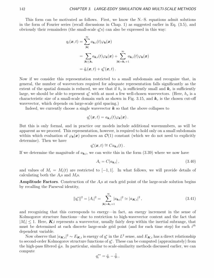
142 CHAPTER 3. LARGE-EDDY SIMULATION AND MULTI-SCALE METHODS
This form can be motivated as follows. First, we know the N.–S. equations admit solutionsin the form of Fourier series (recall discussions in Chap. 1) as suggested earlier in Eq. (3.5), andobviously their remainders (the small-scale q∗i s) can also be expressed in this way:
qi(x, t) =∞∑
|k|
ak,i(t)ϕk(x)
=∑
|k|≤kc
ak,i(t)ϕk(x) +
∞∑
|k|=kc+1
ak,i(t)ϕk(x)
= qi(x, t) + q∗i (x, t) .
Now if we consider this representation restricted to a small subdomain and recognize that, ingeneral, the number of wavevectors required for adequate representation falls significantly as theextent of the spatial domain is reduced, we see that if hs is sufficiently small and kc is sufficientlylarge, we should be able to represent q∗i with at most a few well-chosen wavevectors. (Here, hs is acharacteristic size of a small-scale domain such as shown in Fig. 3.15, and kc is the chosen cut-offwavevector, which depends on large-scale grid spacing.)
Indeed, we currently choose a single wavevector k so that the above collapses to
q∗i (x, t) = ak,i(t)ϕk(x) .
But this is only formal, and in practice our models include additional wavenumbers, as will beapparent as we proceed. This representation, however, is required to hold only on a small subdomainwithin which evaluation of ϕk(x) produces an O(1) constant (which we do not need to explicitlydetermine). Then we have
q∗i (x, t) ∼= Cak,i(t) .
If we determine the magnitude of ak,i, we can write this in the form (3.39) where we now have
Ai = C|ak,i| , (3.40)
and values of Mi = Mi(t) are restricted to [−1, 1]. In what follows, we will provide details ofcalculating both the Ais and Mis.
Amplitude Factors. Construction of the Ais at each grid point of the large-scale solution beginsby recalling the Parseval identity,
‖q∗i ‖2 = |Ai|
2 =
∞∑
|k|=kc+1
|ak,i|2 ≃ |aK,i|
2 , (3.41)
and recognizing that this corresponds to energy—in fact, an energy increment in the sense ofKolmogorov structure functions—due to restriction to high-wavevector content and the fact that|Mi| ≤ 1. Here, K,i represents a wavevector, usually fairly deep within the inertial subrange, thatmust be determined at each discrete large-scale grid point (and for each time step) for each ith
dependent variable.Now observe that |aK,i|2 ∼ EK,i is energy of q∗i in the L2 sense, and EK,i has a direct relationship
to second-order Kolmogorov structure functions of q∗i . These can be computed (approximately) fromthe high-pass filtered qis. In particular, similar to scale-similarity methods discussed earlier, we cancompute
q∗∗i = qi − ˜qi ,
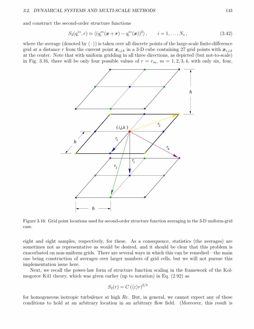
3.2. DYNAMICAL SYSTEMS AND MULTI-SCALE METHODS 143
and construct the second-order structure functions
S2(q∗∗i , r) ≃ 〈(q∗∗i (x + r) − q∗∗i (x))2〉 , i = 1, . . . , Nv , (3.42)
where the average (denoted by 〈 · 〉) is taken over all discrete points of the large-scale finite-differencegrid at a distance r from the current point xi,j,k in a 3-D cube containing 27 grid points with xi,j,k
at the center. Note that with uniform gridding in all three directions, as depicted (but not-to-scale)in Fig. 3.16, there will be only four possible values of r = rm, m = 1, 2, 3, 4, with only six, four,
i,j,k( )
r1
r4
r2
h
r3
r1
h
h
Figure 3.16: Grid point locations used for second-order structure function averaging in the 3-D uniform-gridcase.
eight and eight samples, respectively, for these. As a consequence, statistics (the averages) aresometimes not as representative as would be desired, and it should be clear that this problem isexacerbated on non-uniform grids. There are several ways in which this can be remedied—the mainone being construction of averages over larger numbers of grid cells, but we will not pursue thisimplementation issue here.
Next, we recall the power-law form of structure function scaling in the framework of the Kol-mogorov K41 theory, which was given earlier (up to notation) in Eq. (2.92) as
S2(r) = C (〈ε〉r)2/3
for homogeneous isotropic turbulence at high Re. But, in general, we cannot expect any of theseconditions to hold at an arbitrary location in an arbitrary flow field. (Moreover, this result is

144 CHAPTER 3. LARGE-EDDY SIMULATION AND MULTI-SCALE METHODS
specifically for longitudinal structure functions although it generally holds for transverse ones aswell; but Eq. (3.42) is neither of these.) On the other hand, at least locally with respect to valuesof the independent variables, most quantities in physics can be well represented by a power law.Thus, we replace the above with
S2,i(r) = C (〈ε〉r)β (3.43)
locally in space and time, and for each individual dependent variable, i = 1, . . . , Nv. Now observethat for each value of r we can compute S2,i(r) if we know 〈ε〉, and this can be obtained directlyfrom its definition, Eq. (1.53), applied to the high-pass filtered qi (a form of deconvolution [198])and averaged over the 27 grid points centered on the (i, j, k) point indicated in Fig. 3.16. Then thegeneral exponent β and the constant C in Eq. (3.43) can be found using a least-squares minimizationof the form find β and C such that
4∑
m=1
[S2,i(q
∗∗i , rm) − C (〈ε∗∗〉rm)β
]2
is a minimum, where the values of the S2,i are directly calculated from the definition, Eq. (3.42),and are averaged over the number of entries for each rm. Clearly, this minimization problem canbe expressed in terms of simple closed-form analytical formulas due to use of the power-law form.Hence, even though this computation must be done at every resolved-scale grid point, at everytime step for all dependent variables, there is only quite minimal arithmetic needed. Moreover,calculations at each grid point are independent of all others, so the process is easily parallelized.
Laboratory
Air
Air
Air
Experiment
Figure 3.17: Physical model employed for synthetic-velocity LES of swirling, buoyant plume in an enclosure.
It is worthwhile to study details of the values of β and C that arise from this formulation duringsynthetic-velocity LES calculations that employ all of the above noted aspects. McDonough andYang [72] have reported one such calculation which we summarize here. The physical problem, thedomain of which is sketched in Fig. 3.17, consisted of a turbulent, swirling buoyant plume confined
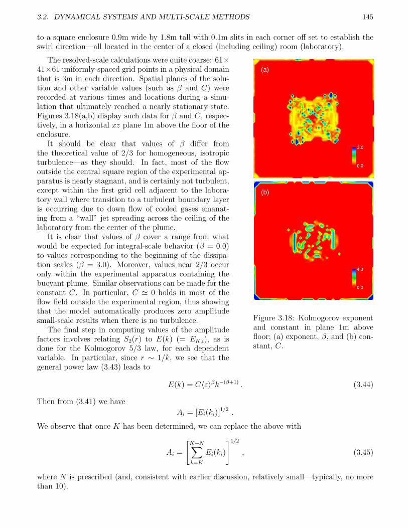
3.2. DYNAMICAL SYSTEMS AND MULTI-SCALE METHODS 145
to a square enclosure 0.9m wide by 1.8m tall with 0.1m slits in each corner off set to establish theswirl direction—all located in the center of a closed (including ceiling) room (laboratory).
3.0
0.0
0.0
4.0
(a)
(b)
Figure 3.18: Kolmogorov exponentand constant in plane 1m abovefloor; (a) exponent, β, and (b) con-stant, C.
The resolved-scale calculations were quite coarse: 61×41×61 uniformly-spaced grid points in a physical domainthat is 3m in each direction. Spatial planes of the solu-tion and other variable values (such as β and C) wererecorded at various times and locations during a simu-lation that ultimately reached a nearly stationary state.Figures 3.18(a,b) display such data for β and C, respec-tively, in a horizontal xz plane 1m above the floor of theenclosure.
It should be clear that values of β differ fromthe theoretical value of 2/3 for homogeneous, isotropicturbulence—as they should. In fact, most of the flowoutside the central square region of the experimental ap-paratus is nearly stagnant, and is certainly not turbulent,except within the first grid cell adjacent to the labora-tory wall where transition to a turbulent boundary layeris occurring due to down flow of cooled gases emanat-ing from a “wall” jet spreading across the ceiling of thelaboratory from the center of the plume.
It is clear that values of β cover a range from whatwould be expected for integral-scale behavior (β = 0.0)to values corresponding to the beginning of the dissipa-tion scales (β = 3.0). Moreover, values near 2/3 occuronly within the experimental apparatus containing thebuoyant plume. Similar observations can be made for theconstant C. In particular, C ≃ 0 holds in most of theflow field outside the experimental region, thus showingthat the model automatically produces zero amplitudesmall-scale results when there is no turbulence.
The final step in computing values of the amplitudefactors involves relating S2(r) to E(k) (= EK,i), as isdone for the Kolmogorov 5/3 law, for each dependentvariable. In particular, since r ∼ 1/k, we see that thegeneral power law (3.43) leads to
E(k) = C〈ε〉βk−(β+1) . (3.44)
Then from (3.41) we have
Ai = [Ei(ki)]1/2 .
We observe that once K has been determined, we can replace the above with
Ai =
[K+N∑
k=K
Ei(ki)
]1/2
, (3.45)
where N is prescribed (and, consistent with earlier discussion, relatively small—typically, no morethan 10).

146 CHAPTER 3. LARGE-EDDY SIMULATION AND MULTI-SCALE METHODS
Currently, we calculate K locally in both space and time by finding the Taylor microscale lengthin each resolved-scale grid cell using Eq. (1.56):
λ =
[ν〈|u′|2〉
ε
]1/2
.
Then for each separate velocity component we calculate
λi ≃
[ν〈u∗∗ 2
i 〉
〈ε〉
]1/2
, i = 1, 2, 3 , (3.46)
where u∗∗i is the high-pass filtered ith velocity component. Then the wavevector components are
1/λi, resulting in
K =
[3∑
i=1
(1
λi
)2]1/2
. (3.47)
Observe that working with individual velocity components and calculating component λis removesany need for homogeneity and/or isotropy assumptions. Our only assumption has been that thelocal in space and time physics (represented as a “general” second-order structure function) can bereasonably well approximated with a power law.
Temporal Fluctuations. Our next task is to find formulas for the Mis. We remark that inthe earliest synthetic-velocity models produced by McDonough and students, these were calculatedfrom linear combinations of logistic maps, as analyzed in detail in [136] and in Hylin [206]. Thisapproach was motivated by an epithet of Frisch [80], mentioned earlier, “poor man’s Navier–Stokesequation,” applied to a quadratic map that can be transformed to a logistic map, and also bythe success, demonstrated by Mukerji et al. [44], in fitting physical chaotic measurements to linearcombinations of logistic maps. It was, however, later discovered by the present author in analyzingresults containing heat transfer in addition to fluid flow, that this approach could not be guaranteedto work. Beyond that is the fact that it is rather ad hoc and difficult to justify, beyond the factthat it seemed to work in some specific situations.
This motivated McDonough and Huang [81] to seek a replacement for the logistic map as thesource of small-scale temporal fluctuations, especially in problems where additional physics (com-bustion chemistry and heat transfer in the cited reference) must be modeled. The approach takenwas to begin with a Galerkin representation of the N.–S. equations such as Eqs. (1.42) and (1.44)(initially in 2D) and any others needed for complete specification of problem physics. This was sim-plified to a Leray-projected form not including pressure gradient terms, and the result was writtenfor a single wavevector for each momentum equation (and other equations, as appropriate). In thecase of the 3-D N.–S. equations, the Fourier representation of, e.g., the x-momentum equation is
∑
ℓ
aℓϕℓ +∑
ℓ,m
(ℓ1 + m1)aℓamϕℓϕm +∑
ℓ,m
(ℓ2 + m2)aℓamϕℓϕm
+∑
ℓ,m
(ℓ3 + m3)aℓamϕℓϕm = −1
Re
(∑
ℓ
|ℓ|2aℓϕℓ
),
and forming the Galerkin inner product with ϕk yields
ak +∑
ℓ,m
A(1)kℓmaℓam +
∑
ℓ,m
B(1)kℓmbℓam +
∑
ℓ,m
C(1)kℓmcℓam = −
C|k|2
Reak ,

3.2. DYNAMICAL SYSTEMS AND MULTI-SCALE METHODS 147
where, for example,
A(1)kℓm ≡ (ℓ1 + m1)
∫
Ω
ϕkϕℓϕm dx .
Then restricting the above to a single wavenumber and writing the result for all three momentumequations leads to
a + A(1)a2 + B(1)ab + C(1)ac =|k|2
Rea ,
b + A(2)ab + B(2)b2 + C(2)bc =|k|2
Reb ,
c + A(3)ab + B(3)bc + C(3)c2 =|k|2
Rec .
These equations are numerically integrated using simple Euler methods (usually forward, but some-times backward for passive scalars), and the result is subjected to two transformations, one due toMcDonough and Huang [81, 82] to introduce the logistic map, and a second due to May [193] toobtain the usual logistic-map scaling of the bifurcation parameters. The result is a true “poor-man’sNavier–Stokes equation:”
a(n+1) = β1a(n)(1 − a(n)
)+ γ12a
(n)b(n) + γ13a(n)c(n) , (3.48a)
b(n+1) = β2b(n)(1 − b(n)
)+ γ21a
(n)b(n) + γ23b(n)c(n) , (3.48b)
c(n+1) = β3c(n)(1 − c(n)
)+ γ31a
(n)c(n) + γ32b(n)c(n) , (3.48c)
where the βis and γijs, i, j = 1, 2, 3, i 6= j, are bifurcation parameters.We remark that one should be concerned about the large number of bifurcation parameters
and how they might be evaluated—is this the turbulence closure problem in just another form?But one readily sees from details of the derivation of Eqs. (3.48) given in 2D in [81, 82] that allof these parameters can be directly related to physical variables which, in turn, can be calculatedfrom the high-pass filtered large-scale solution as has already been done in constructing the Ais. Inparticular, the transformations of [81, 82] and [193] show that
βi = 4
(1 −
τ |k|2
Rei
), i = 1, 2, 3 , (3.49)
where in the context of SGS models the Rei are small-scale component Reynolds numbers definedas
Rei ≡h2|∂u∗∗
i /∂xi|
ν,
with no Einstein summation and h being the discretization step size for the large-scale numericalapproximation. Also, for example,
γ21 ≡ τA(2) = τA(2)kℓm = τA
(2)kℓm ≡ (ℓ2 + m1)
∫
Ω
ϕkϕℓϕm dx . (3.50)
In Eqs. (3.49) and (3.50) τ is the small-scale time scale, obtained in dimensional form as thereciprocal strain rate norm of the high-pass filtered resolved-scale velocity. McDonough et al. [207]show that it is possible to estimate the γijs by τ∂u∗∗
j /∂xi, and there are other possible efficientapproximations. Thus, up to implementational details, we can consider the βis and γijs known ateach large-scale grid point, and for each instant of time—independent of any “adjustable constants.”
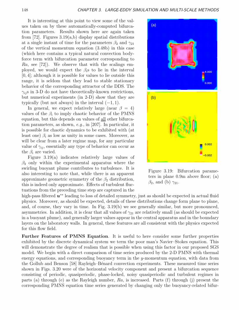
148 CHAPTER 3. LARGE-EDDY SIMULATION AND MULTI-SCALE METHODS
4.000
0.000
(a)
0.002
−0.002
(b)
Figure 3.19: Bifurcation parame-ters in plane 0.9m above floor; (a)β2, and (b) γ21.
It is interesting at this point to view some of the val-ues taken on by these automatically-computed bifurca-tion parameters. Results shown here are again takenfrom [72]. Figures 3.19(a,b) display spatial distributionsat a single instant of time for the parameters β2 and γ21
of the vertical momentum equation (3.48b) in this case(which here contains a typical natural convection body-force term with bifurcation parameter corresponding toRa, see [72]). We observe that with the scalings em-ployed, we would expect the βis to lie in the interval[0, 4]; although it is possible for values to lie outside thisrange, it is seldom that they lead to stable stationarybehavior of the corresponding attractor of the DDS. Theγijs in 3-D do not have theoretically-known restrictions,but numerical experiments (in 2-D) show that they aretypically (but not always) in the interval (−1, 1).
In general, we expect relatively large (near β = 4)values of the βi to imply chaotic behavior of the PMNSequation, but this depends on values of all other bifurca-tion parameters, as shown, e.g., in [207]. In particular, itis possible for chaotic dynamics to be exhibited with (atleast one) βi as low as unity in some cases. Moreover, aswill be clear from a later regime map, for any particularvalue of γij, essentially any type of behavior can occur asthe βi are varied.
Figure 3.19(a) indicates relatively large values ofβ2 only within the experimental apparatus where theswirling buoyant plume contributes to turbulence. It isalso interesting to note that, while there is an apparentapproximate geometric symmetry of the β2 distribution,this is indeed only approximate. Effects of turbulent fluc-tuations from the preceding time step are captured in thehigh-pass filtered u∗∗ leading to loss of detailed symmetry, just as should be expected in actual fluidphysics. Moreover, as should be expected, details of these distributions change form plane to plane,and, of course, they vary in time. In Fig. 3.19(b) we see generally similar, but more pronounced,asymmetries. In addition, it is clear that all values of γ21 are relatively small (as should be expectedin a buoyant plume), and generally larger values appear in the central apparatus and in the boundarylayers on the laboratory walls. In general, these features are all consistent with the physics expectedfor this flow field.
Further Features of PMNS Equation. It is useful to here consider some further propertiesexhibited by the discrete dynamical system we term the poor man’s Navier–Stokes equation. Thiswill demonstrate the degree of realism that is possible when using this factor in our proposed SGSmodel. We begin with a direct comparison of time series produced by the 2-D PMNS with thermalenergy equations, and corresponding buoyancy term in the y-momentum equation, with data fromthe Gollub and Benson [58] Rayleigh–Benard convection experiments. These measured time seriesshown in Figs. 3.20 were of the horizontal velocity component and present a bifurcation sequenceconsisting of periodic, quasiperiodic, phase-locked, noisy quasiperiodic and turbulent regimes inparts (a) through (e) as the Rayleigh number, Ra, is increased. Parts (f) through (j) present thecorresponding PMNS equation time series generated by changing only the buoyancy-related bifur-
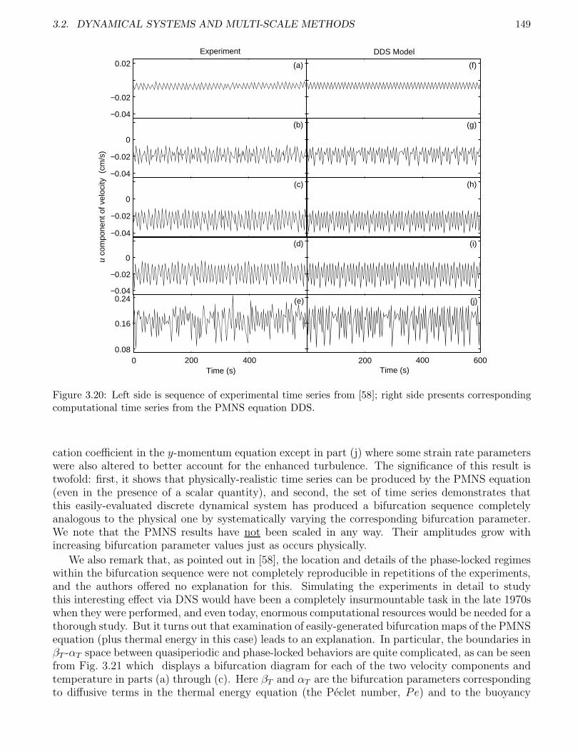
3.2. DYNAMICAL SYSTEMS AND MULTI-SCALE METHODS 149
-0.04
-0.02
0
0.02
-0.04
-0.02
0
0.02
-0.04
-0.02
0
0.02
-0.04
-0.02
0
0.02
0.08
0.16
0.24
Experiment DDS Model
600
600
0 200 400
0 200 400
0.02
0
−0.02
−0.04
0.08
0.16
0.24
200 400 600
u co
mpo
nent
of v
eloc
ity (
cm/s
)
Time (s) Time (s)400200
−0.04
−0.02
−0.04
−0.02
0
−0.04
−0.02
0
(a)
(b)
(c)
(d)
(e)
(f)
(g)
(h)
(i)
(j)
0
Figure 3.20: Left side is sequence of experimental time series from [58]; right side presents correspondingcomputational time series from the PMNS equation DDS.
cation coefficient in the y-momentum equation except in part (j) where some strain rate parameterswere also altered to better account for the enhanced turbulence. The significance of this result istwofold: first, it shows that physically-realistic time series can be produced by the PMNS equation(even in the presence of a scalar quantity), and second, the set of time series demonstrates thatthis easily-evaluated discrete dynamical system has produced a bifurcation sequence completelyanalogous to the physical one by systematically varying the corresponding bifurcation parameter.We note that the PMNS results have not been scaled in any way. Their amplitudes grow withincreasing bifurcation parameter values just as occurs physically.
We also remark that, as pointed out in [58], the location and details of the phase-locked regimeswithin the bifurcation sequence were not completely reproducible in repetitions of the experiments,and the authors offered no explanation for this. Simulating the experiments in detail to studythis interesting effect via DNS would have been a completely insurmountable task in the late 1970swhen they were performed, and even today, enormous computational resources would be needed for athorough study. But it turns out that examination of easily-generated bifurcation maps of the PMNSequation (plus thermal energy in this case) leads to an explanation. In particular, the boundaries inβT -αT space between quasiperiodic and phase-locked behaviors are quite complicated, as can be seenfrom Fig. 3.21 which displays a bifurcation diagram for each of the two velocity components andtemperature in parts (a) through (c). Here βT and αT are the bifurcation parameters correspondingto diffusive terms in the thermal energy equation (the Peclet number, Pe) and to the buoyancy
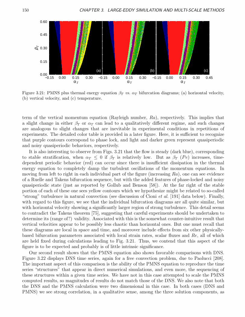
150 CHAPTER 3. LARGE-EDDY SIMULATION AND MULTI-SCALE METHODS
0.15
0.30
0.45
0.60
0.000.00 0.15 0.30 0.00 0.15 0.30 0.00 0.15 0.30−0.15 −0.15 −0.15 0.45
βT
αT
(a) (b) (c)
αT αT
Figure 3.21: PMNS plus thermal energy equation βT vs. αT bifurcation diagrams; (a) horizontal velocity,(b) vertical velocity, and (c) temperature.
term of the vertical momentum equation (Rayleigh number, Ra), respectively. This implies thata slight change in either βT or αT can lead to a qualitatively different regime, and such changesare analogous to slight changes that are inevitable in experimental conditions in repetitions ofexperiments. The detailed color table is provided in a later figure. Here, it is sufficient to recognizethat purple contours correspond to phase lock, and light and darker green represent quasiperiodicand noisy quasiperiodic behaviors, respectively.
It is also interesting to observe from Figs. 3.21 that the flow is steady (dark blue), correspondingto stable stratification, when αT ≤ 0 if βT is relatively low. But as βT (Pe) increases, time-dependent periodic behavior (red) can occur since there is insufficient dissipation in the thermalenergy equation to completely damp the turbulent oscillations of the momentum equations. Inmoving from left to right in each individual part of the figure (increasing Ra), one can see evidenceof a Ruelle and Takens bifurcation sequence, but with the added features of phase-locked and noisyquasiperiodic state (just as reported by Gollub and Benson [58]). At the far right of the stableportion of each of these one sees yellow contours which we hypothesize might be related to so-called“strong” turbulence in natural convection (see discussion of Cioni et al. [191] data below). Finally,with regard to this figure, we see that the individual bifurcation diagrams are all quite similar, butwith horizontal velocity showing a significantly larger region of strong turbulence. This detail seemsto contradict the Takens theorem [75], suggesting that careful experiments should be undertaken todetermine its (range of?) validity. Associated with this is the somewhat counter-intuitive result thatvertical velocities appear to be possibly less chaotic than horizontal ones. But one must recall thatthese diagrams are local in space and time, and moreover include effects from six other physically-based bifurcation parameters associated with local strain rates, scalar fluxes and Re, all of whichare held fixed during calculations leading to Fig. 3.21. Thus, we contend that this aspect of thefigure is to be expected and probably is of little intrinsic significance.
Our second result shows that the PMNS equation also shows favorable comparisons with DNS.Figure 3.22 displays DNS time series, again for a free convection problem, due to Paolucci [208].The important aspect of this comparison is the ability of the PMNS equation to reproduce the timeseries “structures” that appear in direct numerical simulations, and even more, the sequencing ofthese structures within a given time series. We have not in this case attempted to scale the PMNScomputed results, so magnitudes of results do not match those of the DNS. We also note that boththe DNS and the PMNS calculation were two dimensional in this case. In both cases (DNS andPMNS) we see strong correlation, in a qualitative sense, among the three solution components, as
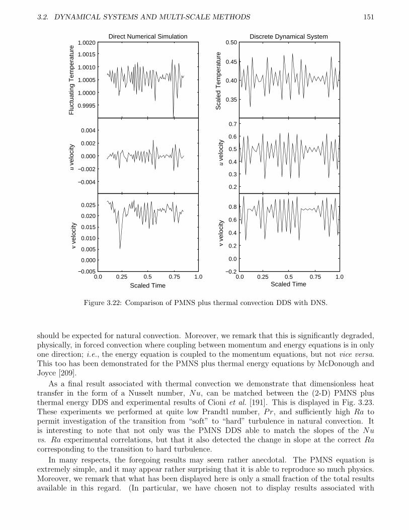
3.2. DYNAMICAL SYSTEMS AND MULTI-SCALE METHODS 151
Flu
ctua
ting
Tem
pera
ture
u ve
loci
tyv
vel
ocity
0.0 0.5 1.00.25 0.75
−0.004
−0.002
0.000
0.002
0.004
−0.005
0.025
0.000
0.005
0.010
0.015
0.020
0.9995
1.0000
1.0005
1.0010
1.0015
1.0020Direct Numerical Simulation
Scaled Time0.0 0.5 1.00.25 0.75
0.0
−0.2
0.2
0.4
0.6
0.8
0.3
0.2
0.4
0.5
0.6
0.7
0.35
0.40
0.50
0.45
Discrete Dynamical System
Scaled Time
Sca
led
Tem
pera
ture
u ve
loci
tyv
vel
ocity
Figure 3.22: Comparison of PMNS plus thermal convection DDS with DNS.
should be expected for natural convection. Moreover, we remark that this is significantly degraded,physically, in forced convection where coupling between momentum and energy equations is in onlyone direction; i.e., the energy equation is coupled to the momentum equations, but not vice versa.This too has been demonstrated for the PMNS plus thermal energy equations by McDonough andJoyce [209].
As a final result associated with thermal convection we demonstrate that dimensionless heattransfer in the form of a Nusselt number, Nu, can be matched between the (2-D) PMNS plusthermal energy DDS and experimental results of Cioni et al. [191]. This is displayed in Fig. 3.23.These experiments we performed at quite low Prandtl number, Pr, and sufficiently high Ra topermit investigation of the transition from “soft” to “hard” turbulence in natural convection. Itis interesting to note that not only was the PMNS DDS able to match the slopes of the Nuvs. Ra experimental correlations, but that it also detected the change in slope at the correct Racorresponding to the transition to hard turbulence.
In many respects, the foregoing results may seem rather anecdotal. The PMNS equation isextremely simple, and it may appear rather surprising that it is able to reproduce so much physics.Moreover, we remark that what has been displayed here is only a small fraction of the total resultsavailable in this regard. (In particular, we have chosen not to display results associated with
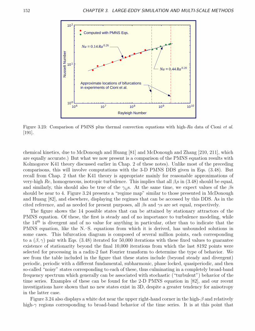
152 CHAPTER 3. LARGE-EDDY SIMULATION AND MULTI-SCALE METHODS
1
10
100
1e+06 1e+07 1e+08 1e+09 1e+10
Nu = 0.14 Ra0.26
Nu = 0.44 Ra0.20
102
101
100
106 107 108 109 1010
Rayleigh Number
Nus
selt
Num
ber
Computed with PMNS Eqs.
Approximate locations of bifurcationsin experiments of Cioni et al.
Figure 3.23: Comparison of PMNS plus thermal convection equations with high-Ra data of Cioni et al.[191].
chemical kinetics, due to McDonough and Huang [81] and McDonough and Zhang [210, 211], whichare equally accurate.) But what we now present is a comparison of the PMNS equation results withKolmogorov K41 theory discussed earlier in Chap. 2 of these notes). Unlike most of the precedingcomparisons, this will involve computations with the 3-D PMNS DDS given in Eqs. (3.48). Butrecall from Chap. 2 that the K41 theory is appropriate mainly for reasonable approximations ofvery-high Re, homogeneous, isotropic turbulence. This implies that all βis in (3.48) should be equal,and similarly, this should also be true of the γijs. At the same time, we expect values of the βsshould be near to 4. Figure 3.24 presents a “regime map” similar to those presented in McDonoughand Huang [82], and elsewhere, displaying the regimes that can be accessed by this DDS. As in thecited reference, and as needed for present purposes, all βs and γs are set equal, respectively.
The figure shows the 14 possible states that can be attained by stationary attractors of thePMNS equation. Of these, the first is steady and of no importance to turbulence modeling, whilethe 14th is divergent and of no value for anything in particular, other than to indicate that thePMNS equation, like the N.–S. equations from which it is derived, has unbounded solutions insome cases. This bifurcation diagram is composed of several million points, each correspondingto a (β, γ) pair with Eqs. (3.48) iterated for 50,000 iterations with these fixed values to guaranteeexistence of stationarity beyond the final 10,000 iterations from which the last 8192 points wereselected for processing in a radix-2 fast Fourier transform to determine the type of behavior. Wesee from the table included in the figure that these states include (beyond steady and divergent)periodic, periodic with a different fundamental, subharmonic, phase locked, quasiperiodic, and thenso-called “noisy” states corresponding to each of these, thus culminating in a completely broad-bandfrequency spectrum which generally can be associated with stochastic (“turbulent”) behavior of thetime series. Examples of these can be found for the 2-D PMNS equation in [82], and our recentinvestigations have shown that no new states exist in 3D, despite a greater tendency for anisotropyin the latter case.
Figure 3.24 also displays a white dot near the upper right-hand corner in the high-β and relativelyhigh-γ regions corresponding to broad-band behavior of the time series. It is at this point that
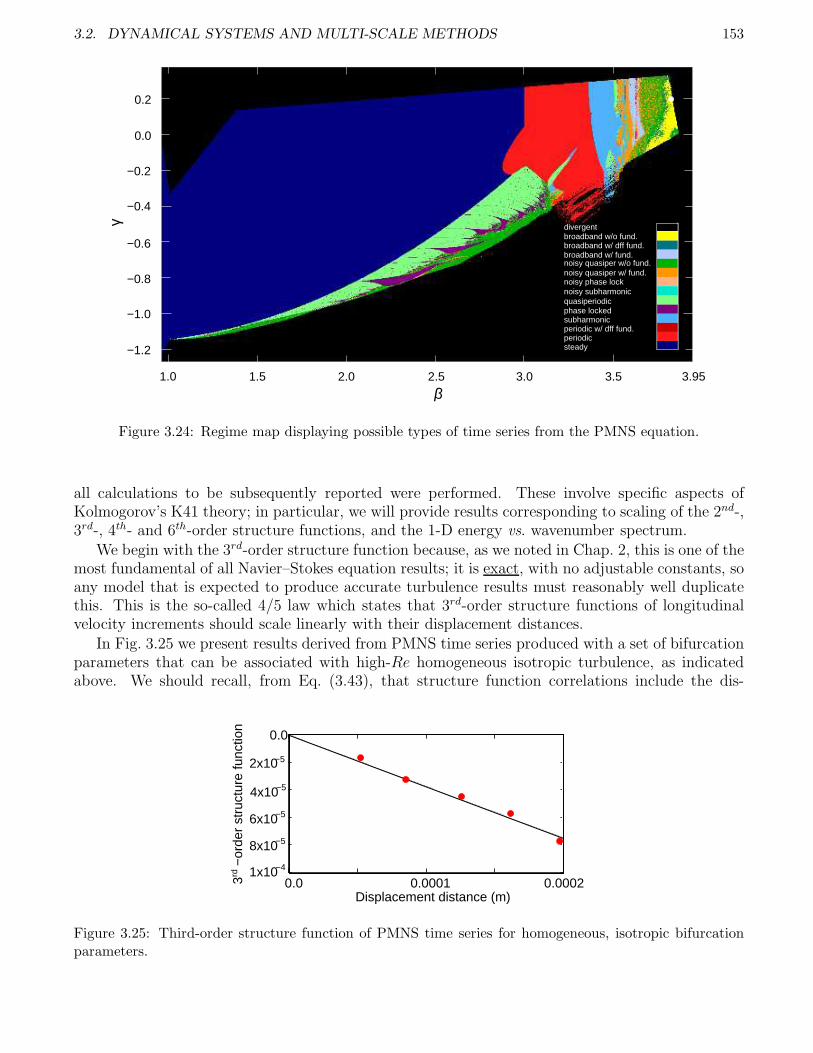
3.2. DYNAMICAL SYSTEMS AND MULTI-SCALE METHODS 153
−0.4
−0.8
−0.6
−1.0
−1.2
−0.2
0.0
0.2
2.0 2.5 3.0 3.51.5 3.951.0β
γ
steadyperiodic
divergentbroadband w/o fund.broadband w/ dff fund.
noisy quasiper w/ fund.noisy phase locknoisy subharmonicquasiperiodicphase lockedsubharmonicperiodic w/ dff fund.
broadband w/ fund.noisy quasiper w/o fund.
Figure 3.24: Regime map displaying possible types of time series from the PMNS equation.
all calculations to be subsequently reported were performed. These involve specific aspects ofKolmogorov’s K41 theory; in particular, we will provide results corresponding to scaling of the 2nd-,3rd-, 4th- and 6th-order structure functions, and the 1-D energy vs. wavenumber spectrum.
We begin with the 3rd-order structure function because, as we noted in Chap. 2, this is one of themost fundamental of all Navier–Stokes equation results; it is exact, with no adjustable constants, soany model that is expected to produce accurate turbulence results must reasonably well duplicatethis. This is the so-called 4/5 law which states that 3rd-order structure functions of longitudinalvelocity increments should scale linearly with their displacement distances.
In Fig. 3.25 we present results derived from PMNS time series produced with a set of bifurcationparameters that can be associated with high-Re homogeneous isotropic turbulence, as indicatedabove. We should recall, from Eq. (3.43), that structure function correlations include the dis-
0.0 0.0001 0.0002
6x10⁻⁵
4x10⁻⁵
2x10⁻⁵
8x10⁻⁵
1x10⁻⁴
0.0
rd 3 −
orde
r st
ruct
ure
func
tion
Displacement distance (m)
Figure 3.25: Third-order structure function of PMNS time series for homogeneous, isotropic bifurcationparameters.
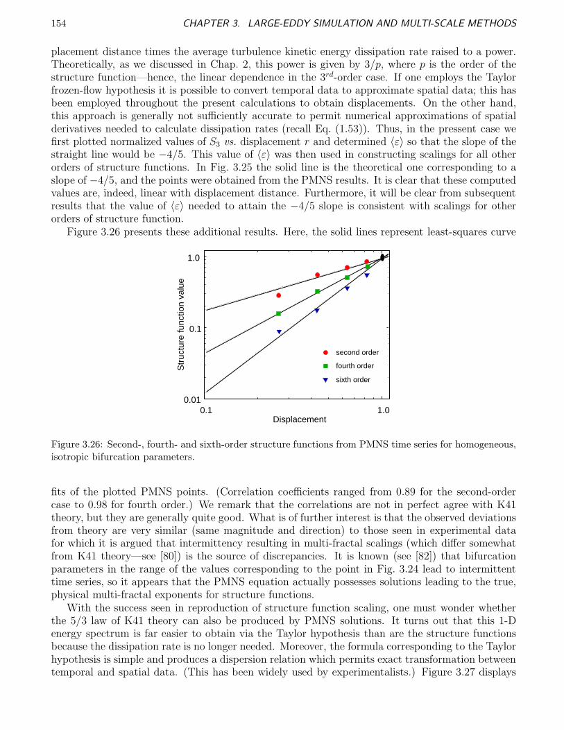
154 CHAPTER 3. LARGE-EDDY SIMULATION AND MULTI-SCALE METHODS
placement distance times the average turbulence kinetic energy dissipation rate raised to a power.Theoretically, as we discussed in Chap. 2, this power is given by 3/p, where p is the order of thestructure function—hence, the linear dependence in the 3rd-order case. If one employs the Taylorfrozen-flow hypothesis it is possible to convert temporal data to approximate spatial data; this hasbeen employed throughout the present calculations to obtain displacements. On the other hand,this approach is generally not sufficiently accurate to permit numerical approximations of spatialderivatives needed to calculate dissipation rates (recall Eq. (1.53)). Thus, in the pressent case wefirst plotted normalized values of S3 vs. displacement r and determined 〈ε〉 so that the slope of thestraight line would be −4/5. This value of 〈ε〉 was then used in constructing scalings for all otherorders of structure functions. In Fig. 3.25 the solid line is the theoretical one corresponding to aslope of −4/5, and the points were obtained from the PMNS results. It is clear that these computedvalues are, indeed, linear with displacement distance. Furthermore, it will be clear from subsequentresults that the value of 〈ε〉 needed to attain the −4/5 slope is consistent with scalings for otherorders of structure function.
Figure 3.26 presents these additional results. Here, the solid lines represent least-squares curve
1.0
0.1
0.011.00.1
Displacement
Str
uctu
re fu
nctio
n va
lue
sixth order
fourth order
second order
Figure 3.26: Second-, fourth- and sixth-order structure functions from PMNS time series for homogeneous,isotropic bifurcation parameters.
fits of the plotted PMNS points. (Correlation coefficients ranged from 0.89 for the second-ordercase to 0.98 for fourth order.) We remark that the correlations are not in perfect agree with K41theory, but they are generally quite good. What is of further interest is that the observed deviationsfrom theory are very similar (same magnitude and direction) to those seen in experimental datafor which it is argued that intermittency resulting in multi-fractal scalings (which differ somewhatfrom K41 theory—see [80]) is the source of discrepancies. It is known (see [82]) that bifurcationparameters in the range of the values corresponding to the point in Fig. 3.24 lead to intermittenttime series, so it appears that the PMNS equation actually possesses solutions leading to the true,physical multi-fractal exponents for structure functions.
With the success seen in reproduction of structure function scaling, one must wonder whetherthe 5/3 law of K41 theory can also be produced by PMNS solutions. It turns out that this 1-Denergy spectrum is far easier to obtain via the Taylor hypothesis than are the structure functionsbecause the dissipation rate is no longer needed. Moreover, the formula corresponding to the Taylorhypothesis is simple and produces a dispersion relation which permits exact transformation betweentemporal and spatial data. (This has been widely used by experimentalists.) Figure 3.27 displays

3.2. DYNAMICAL SYSTEMS AND MULTI-SCALE METHODS 155
a PMNS 1-D energy spectrum on which the k−5/3 slope is indicated. We observe that the integral
0.1 1.0 10. 100. 1000. 10000.10−8
10−6
10−4
10−2
0
100
Wavenumber
Ene
rgy
k−5/3
Figure 3.27: PMNS equation 1-D energy spectrum.
scale is apparent, with approximately two decades of inertial subrange behavior, before some decaytoward dissipation scales is seen. In particular, the PMNS equation is carrying a considerableamount of the physics associated with the full system of N.–S. equations. But, of course, from amodeling standpoint this is only local. At this point one might wonder how a model constructedfrom at most a few wavenumbers could produce results over a wavenumber range such as indicated inthe figure. The “mechanism” for this is the same as occurs in analogous treatments of experimentaltime series. Namely, the longer the time series, the larger the possible range of frequencies thatwill be produced by an FFT of the data—just and immediate consequence of the Nyquist criterionfor signal processing. But this, in turn, implies a large range of wavenumbers, a la the dispersionrelation that corresponds to the Taylor hypothesis.
PMNS Equation Viewed as Pseudodifferential Operator of Navier–Stokes Equations.The preceding results appear to be extremely favorable, and one must ask how such a relativelysimple system of algebraic maps could possibly reproduce so much of the behavior of a theoreticallyvery complicated system of partial differential equations. We will provide an answer to this questionin the present subsection.
The goal of this section is demonstration that Eqs. (3.48) comprise a mathematical object thatis closely related to a time-dependent, nonlinear pseudodifferential operator corresponding to theN.–S. equations. To do this we start with a brief review of the simplest notions associated withpseudodifferential operators; we then use these to show that the PMNS equation arises from ananalogous structure, and then discuss the significance of this result.
Definition 3.2 Let Ω ⊆ Rn and ξ ∈ Rn. Then for u ∈ C∞0 (Ω) a simple (vector) pseudodifferential
operator on Ω can be expressed as (see, e.g., Treves [212])
Pu(x) =1
(2π)n
∫eix·ξp(x, ξ)u(ξ)dξ , (3.51)
where u is the Fourier transform of u:
u(ξ) ≡
∫u(x)e−ix·ξdx .
In (3.51) p(x, ξ) is a smooth (vector) function on Ω × Rn and is called the symbol of the pseudo-differential operator P .
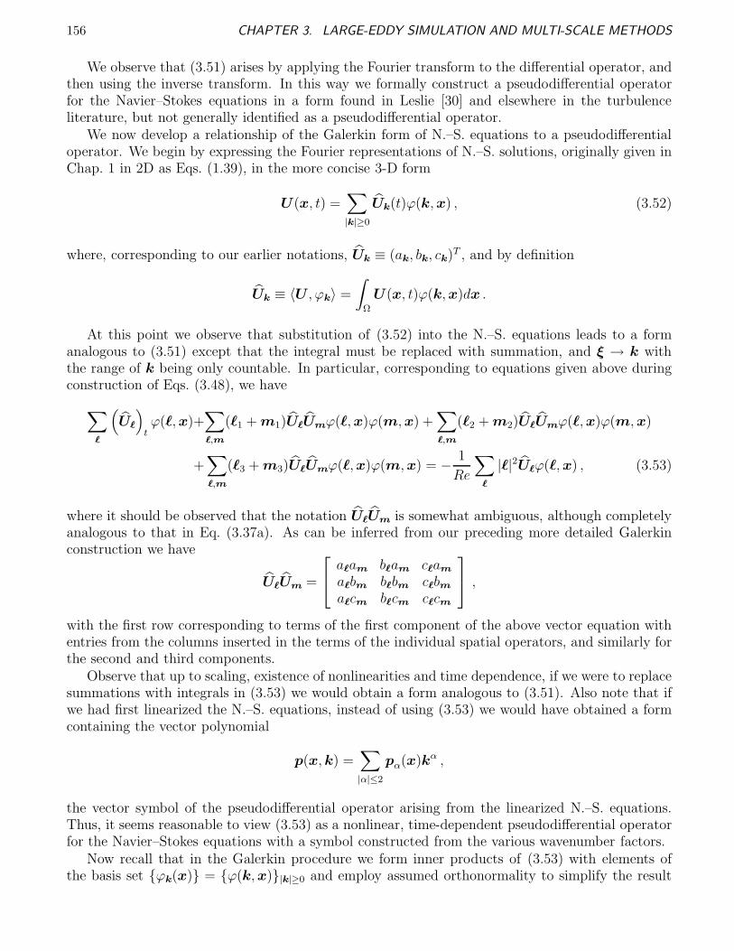
156 CHAPTER 3. LARGE-EDDY SIMULATION AND MULTI-SCALE METHODS
We observe that (3.51) arises by applying the Fourier transform to the differential operator, andthen using the inverse transform. In this way we formally construct a pseudodifferential operatorfor the Navier–Stokes equations in a form found in Leslie [30] and elsewhere in the turbulenceliterature, but not generally identified as a pseudodifferential operator.
We now develop a relationship of the Galerkin form of N.–S. equations to a pseudodifferentialoperator. We begin by expressing the Fourier representations of N.–S. solutions, originally given inChap. 1 in 2D as Eqs. (1.39), in the more concise 3-D form
U(x, t) =∑
|k|≥0
Uk(t)ϕ(k, x) , (3.52)
where, corresponding to our earlier notations, Uk ≡ (ak, bk, ck)T , and by definition
Uk ≡ 〈U , ϕk〉 =
∫
Ω
U(x, t)ϕ(k, x)dx .
At this point we observe that substitution of (3.52) into the N.–S. equations leads to a formanalogous to (3.51) except that the integral must be replaced with summation, and ξ → k withthe range of k being only countable. In particular, corresponding to equations given above duringconstruction of Eqs. (3.48), we have
∑
ℓ
(Uℓ
)tϕ(ℓ, x)+
∑
ℓ,m
(ℓ1 + m1)UℓUmϕ(ℓ, x)ϕ(m, x) +∑
ℓ,m
(ℓ2 + m2)UℓUmϕ(ℓ, x)ϕ(m, x)
+∑
ℓ,m
(ℓ3 + m3)UℓUmϕ(ℓ, x)ϕ(m, x) = −1
Re
∑
ℓ
|ℓ|2Uℓϕ(ℓ, x) , (3.53)
where it should be observed that the notation UℓUm is somewhat ambiguous, although completelyanalogous to that in Eq. (3.37a). As can be inferred from our preceding more detailed Galerkinconstruction we have
UℓUm =
aℓam bℓam cℓam
aℓbm bℓbm cℓbm
aℓcm bℓcm cℓcm
,
with the first row corresponding to terms of the first component of the above vector equation withentries from the columns inserted in the terms of the individual spatial operators, and similarly forthe second and third components.
Observe that up to scaling, existence of nonlinearities and time dependence, if we were to replacesummations with integrals in (3.53) we would obtain a form analogous to (3.51). Also note that ifwe had first linearized the N.–S. equations, instead of using (3.53) we would have obtained a formcontaining the vector polynomial
p(x, k) =∑
|α|≤2
pα(x)kα ,
the vector symbol of the pseudodifferential operator arising from the linearized N.–S. equations.Thus, it seems reasonable to view (3.53) as a nonlinear, time-dependent pseudodifferential operatorfor the Navier–Stokes equations with a symbol constructed from the various wavenumber factors.
Now recall that in the Galerkin procedure we form inner products of (3.53) with elements ofthe basis set ϕk(x) = ϕ(k, x)|k|≥0 and employ assumed orthonormality to simplify the result
3.2. DYNAMICAL SYSTEMS AND MULTI-SCALE METHODS 157
to the form
∂Uk
∂t+
|k|2
ReUk +
∑
ℓ,m
AkℓmUℓUm +∑
ℓ,m
BkℓmUℓUm +∑
ℓ,m
CkℓmUℓUm = 0 ,
k = 0, 1, . . . ,∞ .
Although this is no longer in the form (3.51) because the ϕ(k, x) have been integrated (to formAkℓm, etc.), it does represent a direct simplification of (3.53)—one that is essential if a solution
consisting of the Uk is to be obtained. Moreover, the final form of the PMNS equation (3.48) followsimmediately from this via discretization in time, as shown in the preceding subsection. Hence, itappears reasonable to view the PMNS equation as being closely related to a simple discretizationof a microlocal (because only a single wavevector is retained) pseudodifferential operator for theN.–S. equations.
The importance of the relationship between the PMNS equation and pseudodifferential opera-tors of the N.–S. equations cannot be overemphasized. For simple linear PDEs pseudodifferentialoperators provide an algebra leading to exact solutions in some cases, and at least simplified analy-sis in more complicated situations. In any case, estimating the integral operator on the right-handside of (3.51) is typically far more tractable than attempting to estimate the original differentialoperators, especially in the context of microlocal analyses employed herein and elsewhere. In thenonlinear, time-dependent case being treated here, this is true locally (in physical and/or wavenum-ber space) via microlocal analysis, and it also leads to an efficient computational tool. As we havedemonstrated in the preceding subsection, and in various of the cited references, we are already em-ploying the PMNS equation both as a part of SGS models for LES and for “curve fitting” chaotic(presumably turbulent) experimental flow data. Identification of the PMNS equation with a pseu-dodifferential operator of the N.–S. equations provides an explanation for the previous (seeminglysomewhat fortuitous) success of the curve fits (see [45]) and suggests its use should be valuable inconstructing high-fidelity SGS models for LES, as has been initiated in [72]. Moreover, in this latterapplication it provides a means to introduce mathematical rigor (via microlocal analysis) into studyof SGS models.
Application of Multi-Scale Formalism to Produce Complete Solution. During eachresolved-scale time step Eqs. (3.48) are iterated a number of times corresponding to formal in-tegration of the small-scale equations across the large-scale time step. This number is set by usinga small-scale time scale obtained as τ ≡ 1/‖S∗∗‖, as noted above. The result of this is evaluationof a discrete dynamical system directly related to the N.–S. equations, but restricted to a singlewavevector (per dependent variable), and associated with the Mis of Eq. (3.39) as
M1 = a , M2 = b , M3 = c . (3.54)
But these “velocity components” require rescaling; recall that the Mis are restricted to [−1, 1]to make sense of use of the amplitude factors, Ais. In addition, these velocity components are notdivergence free (just as is the case for velocity components computed from essentially any form of(3.37) on any scale). Thus, after calculating q∗i (x, t), i = 1, . . . , Nv, of Eq. (3.40) at all resolved-scalegrid points, we must project the portion of this solution vector corresponding to the velocity fieldonto a divergence-free subspace by first solving a (pseudo-) pressure Poisson equation,
∆p∗ =∇·u∗
∆t, (3.55)
and then projecting the velocity field in the usual way via
u∗ = u∗ − ∆t p∗x , v∗ = v∗ − ∆t p∗y , w∗ = w∗ − ∆t p∗z . (3.56)

158 CHAPTER 3. LARGE-EDDY SIMULATION AND MULTI-SCALE METHODS
These are the fluctuating (small-scale) velocity components on the large-scale grid at time leveln + 1. Furthermore, as is well known, p∗ provides a reasonable approximation to the small-scalefluctuating pressure if Re is large (despite the fact—or, maybe because of it—that p∗ is actuallya velocity potential). See McDonough [204] for more detailed discussions of projection methodsapplied to the incompressible N.–S. equations.
At this point both large- and small-scale solution compoments are available at time level n + 1,and we are now ready to consider precisely how to use the SGS quantities in the context of a formalmulti-scale procedure. We again remind the reader that LES is intrinsically a multi-scale approachdue to the basic decomposition of dependent variables:
qi(x, t) = qi(x, t) + q∗i (x, t) , i = 1, 2, . . . , Nv . (3.57)
Indeed, as should be clear from the preceding treatment, both qi and q∗i have been constructed suchthat each serves as at least a consistent approximation to the corresponding Hilbert (sub)spacequantities. Up to now this has been implicit for qi, and we here provide a basic description of thispart of the method.
We earlier noted that the synthetic-velocity approach presented here begins with a formulationnot too different from ATD; in fact, the large-scale equations are those of ATD. Thus, we formallysolve
(U + U ∗)t + ∇·((U + U ∗)2
)= −∇(P + P ∗) + ν∆(U + U ∗) , (3.58a)
∇·(U + U ∗) = 0 , (3.58b)
for U with U ∗ computed as given in the preceding analyses. The same treatment is also applied toany additional quantities related to the physics of a particular problem. Formal numerical-analyticconsistency (but not necessarily accuracy) of this approach is obvious if a consistent discretizationis applied to (3.58) because U ∗, and P ∗ → 0 as ∆t, hi → 0.
But it is well known from a numerical-analytic standpoint that consistency does not implystability (nor vice versa, of course), and it is often observed that small-scale perturbations arisingin multi-scale algorithms lead to destabilization of the underlying numerical method. Beyond thisis yet a separate and subtle issue that occurs for heterogeneous multi-scale algorithms, in general(see [196]), of which the present synthetic-velocity LES is an example. Namely, because the q∗i shave been produced with a completely separate algorithm from that leading to the qis, but at thesame time the qis are required to satisfy the same discrete equations as do the qis, it follows thattime-derivative information is needed for the q∗i s. In particular, if one considers the discrete solutionoperator
qn+1i = qn
i +
∫ tn+1
tnFi(q) dt (3.59)
for the large-scale part of the solution, and takes this to be the same as the complete solutionoperator
qn+1i = qn
i +
∫ tn+1
tnFi(q) dt ,
then since from (3.57)
qn+1i = q n+1
i + q∗n+1i ,
we see that
dq = d q + dq∗
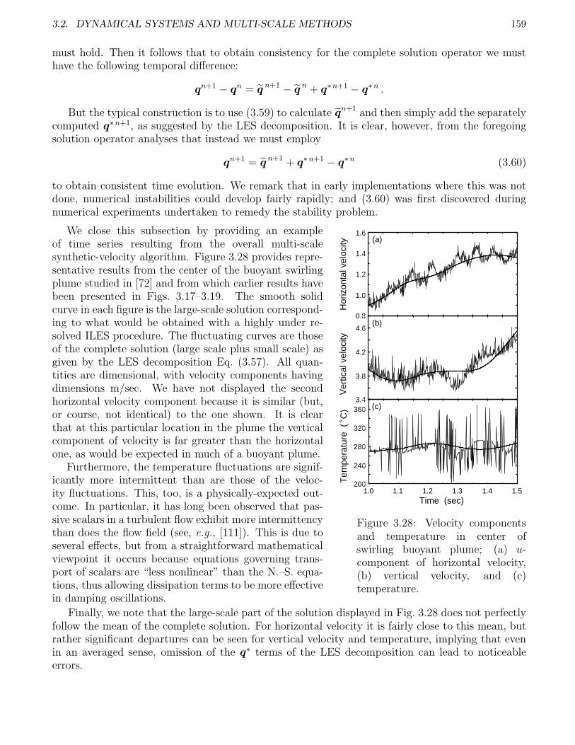
3.2. DYNAMICAL SYSTEMS AND MULTI-SCALE METHODS 159
must hold. Then it follows that to obtain consistency for the complete solution operator we musthave the following temporal difference:
qn+1 − qn = qn+1 − q
n + q∗n+1 − q∗n .
But the typical construction is to use (3.59) to calculate qn+1 and then simply add the separately
computed q∗n+1, as suggested by the LES decomposition. It is clear, however, from the foregoingsolution operator analyses that instead we must employ
qn+1 = qn+1 + q∗n+1 − q∗n (3.60)
to obtain consistent time evolution. We remark that in early implementations where this was notdone, numerical instabilities could develop fairly rapidly; and (3.60) was first discovered duringnumerical experiments undertaken to remedy the stability problem.
1.0 1.21.1 1.41.3 1.5
0.8
1.0
1.2
1.4
1.6
3.4
3.8
4.2
4.6
0.8
0.9
1
1.1
1.2
1.3
1.4
1.5
1.6
1 1.05 1.1 1.15 1.2 1.25 1.3 1.35 1.4 1.45 1.5
3.4
3.6
3.8
4
4.2
4.4
4.6
4.8
1 1.05 1.1 1.15 1.2 1.25 1.3 1.35 1.4 1.45 1.5
200
240
280
320
360
200
220
240
260
280
300
320
340
360
380
1 1.05 1.1 1.15 1.2 1.25 1.3 1.35 1.4 1.45 1.5
Time (sec)
Tem
pera
ture
( C
)°
V
ertic
al v
eloc
ityH
oriz
onta
l vel
ocity (a)
(b)
(c)
Figure 3.28: Velocity componentsand temperature in center ofswirling buoyant plume; (a) u-component of horizontal velocity,(b) vertical velocity, and (c)temperature.
We close this subsection by providing an exampleof time series resulting from the overall multi-scalesynthetic-velocity algorithm. Figure 3.28 provides repre-sentative results from the center of the buoyant swirlingplume studied in [72] and from which earlier results havebeen presented in Figs. 3.17–3.19. The smooth solidcurve in each figure is the large-scale solution correspond-ing to what would be obtained with a highly under re-solved ILES procedure. The fluctuating curves are thoseof the complete solution (large scale plus small scale) asgiven by the LES decomposition Eq. (3.57). All quan-tities are dimensional, with velocity components havingdimensions m/sec. We have not displayed the secondhorizontal velocity component because it is similar (but,or course, not identical) to the one shown. It is clearthat at this particular location in the plume the verticalcomponent of velocity is far greater than the horizontalone, as would be expected in much of a buoyant plume.
Furthermore, the temperature fluctuations are signif-icantly more intermittent than are those of the veloc-ity fluctuations. This, too, is a physically-expected out-come. In particular, it has long been observed that pas-sive scalars in a turbulent flow exhibit more intermittencythan does the flow field (see, e.g., [111]). This is due toseveral effects, but from a straightforward mathematicalviewpoint it occurs because equations governing trans-port of scalars are “less nonlinear” than the N.–S. equa-tions, thus allowing dissipation terms to be more effectivein damping oscillations.
Finally, we note that the large-scale part of the solution displayed in Fig. 3.28 does not perfectlyfollow the mean of the complete solution. For horizontal velocity it is fairly close to this mean, butrather significant departures can be seen for vertical velocity and temperature, implying that evenin an averaged sense, omission of the q∗ terms of the LES decomposition can lead to noticeableerrors.
160 CHAPTER 3. LARGE-EDDY SIMULATION AND MULTI-SCALE METHODS
Pseudo-Language Algorithm for Multi-Scale Synthetic-Velocity LES. We will end thistreatment of the multi-scale, dynamical-systems-based approach to LES by providing a coarse-grained pseudo-language algorithm from which, in principle, computer code can be written. Wenote, however, that considerable additional effort will be needed to produce a complete operationalprogram. The present algorithm represents only an outline of the overall process.
Algorithm 3.2 (Multi-Scale, Synthetic-Velocity LES). Suppose n resolved-scale time steps havebeen completed. To calculate n + 1 time-level results, perform the following steps.
1. Solve Eq. (3.58a) for Un+1
by any valid CFD method (see, e.g., McDonough [204] for various
possibilities) using values of U ∗ from the preceding time step. Note that the Un+1
velocityfield must be divergence free before proceeding to the next step.
2. Construct the SGS contribution U ∗. Note that this can be done with either the new timelevel U
n+1velocity field, or with the previous time-level result U
n. (Use of the latter permits
extensive parallelization of the overall algorithm.)
a. High-pass filter U to obtain U ∗∗.
b. Determine turbulent time scale at each large-scale grid point using τ = 1/‖S∗∗‖.
c. Calculate Taylor microscale length at each grid point via Eq. (3.46).
d. For every grid point at which τ > ∆t and λi > hi ∀ i = 1, 2, 3, set all q∗i = 0, and proceedto next grid point. Here, ∆t is the large-scale time step, and the hi are the large-scalespatial discretization step sizes.
e. Compute amplitude factors, Ai, for each solution component using Eqs. (3.43)–(3.47).
f. Evaluate bifurcation parameters of PMNS equation from Eq. (3.49) and (usually, a sur-rogate involving a difference approximation of appropriate high-pass filtered velocity com-ponents for) Eq. (3.50).
g. Set Nmax = ∆t/τ + 1, and iterate the PMNS equation for Nmax iterations. Note: Nmax
will not, in general, be the same at all grid points.
h. Obtain provisional q∗i , i = 1, . . . , Nv, from Eq. (3.39).
i. Project entire q∗i velocity field onto divergence-free subspace via Eqs. (3.55) and (3.56).
3. Employ Eq. (3.60) to obtain the complete n + 1 time-level solution.
There are several points to be made regarding this algorithm. First, an implementation is inexistence and was used to produce Figs. 3.18, 3.19 and 3.28, as already indicated. In fact, variousother turbulence problems have also been solved with this code; but it is still under development, andlittle has been published in the archival literature. Second, as noted in step 1 of the algorithm, the
time level Un+1
velocity field must be divergence free before proceeding to the rest of the algorithm(among other things, making solution algorithms of the form of SIMPLE not very appropriate).This is the only part of the algorithm devoted to mass conservation of large-scale results. Moreover,
if Un+1
used in step 2 is not divergence free, turbulence in the small scales will have been generatedwith an incorrect large-scale velocity field.
The third point specifically concerns step 2. We have indicated that either time level n or n + 1large-scale velocity fields can be used in this step. The reason for this flexibility is that we can viewthe small-scale calculations in two, nearly equivalent, ways. If we look on this as simply an explicit
time integration continuing from the preceding time step, then use of Un
is appropriate. On theother hand, we can view this overall multi-scale algorithm as a predictor-corrector method in which

3.2. DYNAMICAL SYSTEMS AND MULTI-SCALE METHODS 161
we make a rough prediction (not including high-wavenumber content) via large-scale calculations atthe beginning of a new time step, and then correct this with small-scale, high-wavenumber results.
In this context Un+1
would be preferred. It should be clear, however, that detailed results fromthese two approaches cannot be identical; but we should expect their statistics to be the same(under the assumption that the two different solutions lie on the same N.–S. attractor).
We further note that the nature of step 2.d is such as to detect under resolution in both spaceand time, and to generate small-scale solutions if this occurs in either (or both). Conversely, if∆t and the his are sufficiently small (compared with respective inertial range scales), then thecalculations correspond to DNS, and no SGS models are needed. In addition, it should be clear
from step 2.g that independent of whether U ∗∗ is based on Un
or Un+1
, we formally integrate thePMNS equation over a large-scale time step. Indeed, solutions to this equation are stored from
the preceding time step and used as initial data at the new time step. Thus, the choice of Un
or
Un+1
directly effects amplitude factors in the small-scale solution representation and bifurcationparameters in the PMNS equation, but it does not effect the small-scale integration process.
Finally, we note that step 2.i is the arithmetically expensive part of the SGS model because itrequires solution of a Poisson equation to impose mass conservation on U ∗. At the same time, thisintroduces global effects into otherwise completely local small-scale solutions (which is desirable).But, as is well know, Poisson equation solves are the expensive part of any incompressible flowsimulation, so we have essentially doubled the total arithmetic over that required for a laminar flowcalculation (on the same grid). On the other hand, total arithmetic is nearly the same for bothlarge and small scales, leading to good load balancing in a parallel computing environment. Hence,in principle, even if only two processors are available, the present algorithm can produce a turbulentsolution in essentially the same wall-clock time as needed for a laminar solution.
3.2.4 Summary of dynamical systems/multi-scale methods
In this section we first provided an elementary discussion of general aspects of dynamical systems,including such notions as attractor, bifurcation, fractal, and strange attractor; and we describedseveral of the more inportant diagnostic tools used in analyzing these objects, including use of powerspectra, phase portraits, etc. We then provided a brief, heuristic overview of multi-scale ideas andthen used these in combination with dynamical systems to develop a synthetic-velocity version oflarge-eddy simulation. The keys to this approach include filtering solutions rather than equations,directly modeling SGS physical quantities instead of their statistics, and finally, explicitly combiningresolved-scale and SGS quantities to produce the entire LES (Hilbert space) representation of flowvariables.
The portions of this analysis that are quite new are first the (formally) single-mode Fourierrepresentations of SGS quantities as a product of an amplitude and a time-dependent oscillation,and second the details by means of which each of these is calculated. Amplitudes are producedas a generalization of Kolmogorov’s K41 theory to power laws for which exponents must be de-termined based on resolved-scale results—a form of deconvolution which removes the homogeneityand isotropy assumptions of the K41 theory. Temporal fluctuations are computed from the poorman’s Navier–Stokes equation, a discrete dynamical system derived from the N.–S. equations viaa Galerkin procedure, and which represents a discretization of microlocalization of a pseudodif-ferential operator of the N.–S. equations. We demonstrated that the PMNS equation is able toreplicate both experimental and DNS results, and that it furthermore reproduces the KolmogorovK41 scalings—in fact, display possible multi-fractal effects more like K62 theory. We concluded thatthis type of SGS model shows very good promise for future development, and a pseudo-languagealgorithm was provided for its implementation.
162 CHAPTER 3. LARGE-EDDY SIMULATION AND MULTI-SCALE METHODS
3.3 Summary
This chapter dealt with modern turbulence simulation techniques of the general nature of large-eddysimulation. We presented the usual methods of LES in some detail, beginning with the basic stepsof construction—the LES decomposition, filtering of governing equations, formulating SGS models,and neglecting small-scale results—including treatment of Smagorinsky, dynamic and mixed SGSmodels. Then much more analysis was provided for a very modern synthetic-velocity approach toLES which eliminates some of the shortcomings of the more classical approaches. The key aspectsof this new approach appeal to rigorous mathematics of PDEs and include use of mollificationof large-scale solution components to control aliasing caused by the (deliberately) under-resolvedrepresentations, modeling of SGS dependent variables via extension of Kolmogorov K41 theory anddirect application of dynamical systems in the form of the poor man’s Navier–Stokes equation, andintroduction of multi-scale methods to construct the complete LES decomposition. The result of thiscombination of techniques is one of the first turbulence modeling procedures to explicitly employtheories from dynamical systems which, in the context of the Navier–Stokes equations—becausethese are a dynamical system—correctly establish the mathematical nature of the intriguing andelusive physical phenomenon known as turbulence.
References
[1] G. T. Chapman and M. Tobak. Observations, Theoretical Ideas, and Modeling of TurbulentFlows — Past, Present and Future, in Theoretical Approaches to Turbulence, Dwoyer et al.(eds), Springer-Verlag, New York, pp. 19–49, 1985.
[2] P. Constantin and C. Foias. Navier–Stokes Equations, University of Chicago Press, Chicago,1988.
[3] A. Tsinober. An Informal Introduction to Turbulence, Kluwer Academic Publishers, Dor-drecht, 2001.
[4] L. F. Richardson. Weather Prediction by Numerical Process, Cambridge University Press,1922.
[5] T. von Karman. Some remarks on the statistical theory of turbulence, Proc. 5th Int. Congr.Appl. Mech., Cambridge, MA, 347, 1938.
[6] J. O. Hinze. Turbulence, McGraw-Hill, New York, 1959.
[7] H. Tennekes and J. L. Lumley. A First Course in Turbulence. MIT Press, 1972.
[8] D. Ruelle and F. Takens. On the nature of turbulence. Comm. Math. Phys. 20, 167–192,1971.
[9] S. A. Orszag and G. S. Patterson. Numerical simulation of turbulence: statistical models andturbulence, Lecture Notes in Physics 12, 127–147, Springer-Verlag, Berlin, 1972.
[10] J. W. Deardorff. A numerical study of three-dimensional turbulent channel flow at largeReynolds numbers, J. Fluid Mech. 41, 453, 1970.
[11] B. E. Launder and D. B. Spalding. Mathematical Models of Turbulence, Academic Press,1972.
[12] R. S. Rogallo and P. Moin. Numerical simulation of turbulent flows, Annu. Rev. Fluid Mech.16, 99–137, 1984.
[13] J. Kim, P. Moin and R. Moser. Turbulence statistics in fully developed channel flow at lowReynolds number, J. Fluid Mech. 177, 133–166, 1987.
[14] M. Lesieur. Turbulence in Fluids, Second Revised Edition, Kluwer Academic Press, Dordrecht,1990.
[15] J. Boussinesq. Essai sur la theorie des eaux courantes, Mem. pres. par div. savant a l’Acad.Sci. 23, 1–680, 1877.
163
164 REFERENCES
[16] O. Reynolds. On the dynamical theory of turbulent incompressible viscous fluids and thedetermination of the criterion, Phil. Trans. R. Soc. London A 186, 123–161, 1894.
[17] H. Poincare. Les Methodes Nouvelles de la Mecanique Celeste, Vol. 1–3, Gauthier Villars,Paris, 1899.
[18] E. N. Lorenz. Deterministic nonperiodic flow. J. Atmos. Sci. 20, 130–141, 1963.
[19] L. Prandtl. Bericht uber Untersuchungen zur ausgebildeten Turbulenz, Zs. agnew. Math.Mech. 5, 136–139, 1925.
[20] G. I. Taylor. Statistical theory of turbulence, Proc. Roy. Soc. London A 151, 421–478, 1935.
[21] T. von Karman. On the statistical theory of turbulence, Proc. Nat. Acad. Sci., Wash. 23,98, 1937.
[22] T. von Karman and L. Howarth. On the statistical theory of isotropic turbulence, Proc. Roy.Soc. A, 164, 192, 1938.
[23] N. Weiner. The use of statistical theory in the study of turbulence, Proc. 5th Int. Congr.Appl. Mech., Cambridge, MA, 356, 1938.
[24] J. Leray. Etude de diverses equations integrals non lineaires et de quelques problemes quepose l’hydrodynamique. J. Math. Pures Appl. 12, 1–82, 1933.
[25] J. Leray. Essai sur les mouvemnts d’ un liquide visqueaux que limitent des parois. J. Math.Pures Appl. 13, 331–418, 1934.
[26] A. N. Kolmogorov. The local structure of turbulence in incompressible viscous fluid for verylarge Reynolds number, Dokl. Acad. Nauk. SSSR 30, 9–13, 1941; On degeneration (decay)of isotropic turbulence in an incompressible viscous liquid, Dokl. Acad. Nauk. SSSR 31, 538–540, 1941; Dissipation of energy in locally isotropic turbulence, Dokl. Acad. Nauk. SSSR 32,16–18, 1941.
[27] A. N. Kolmogorov. A refinement of previous hypotheses concerning the local structure ofturbulence in a viscous incompressible fluid at high Reynolds number, J. Fluid Mech. 13,82–85, 1962.
[28] E. Hopf. A mathematical example displaying the features of turbulence, Commun. Pure Appl.Math. 1, 303, 1948.
[29] L. D. Landau and E. M. Lifshitz. Fluid Mechanics (translated by J. B. Sykes and W. H. Reidfrom original Russian published in 1944), Pergamon Press, Oxford, 1959.
[30] D. C. Leslie. Developments in the Theory of Turbulence, Oxford University Press, Oxford,1973.
[31] G. K. Batchelor. Energy decay and self-preserving correlation functions in isotropic turbu-lence, Quart. Appl. Math. 6, 97, 1948.
[32] J. M. Burgers. A mathematical model illustrating the theory of turbulence, Adv. Appl. Mech.1, 171, 1948.
[33] S. Corrsin. An experimental verification of local isotropy, J. Aero. Sci. 16, 757, 1949.

REFERENCES 165
[34] W. Heisenberg. On the theory of statistical and isotropic turbulence, Proc. Roy. Soc. A, 195,402, 1948.
[35] T. von Karman. Progress in the statistical theory of turbulence, Proc. Nat. Acad. Sci., Wash.34, 530, 1948.
[36] A. M. Obukhov. The local structure of atmospheric turbulence, Doklady. Akad. Nauk. SSSR67, 643, 1949.
[37] A. A. Townsend. The measurement of double and triple correlation derivatives in isotropicturbulence, Proc. Camb. Phil. Soc. 43, 560, 1947.
[38] A. M. Yaglom. Homogeneous and isotropic turbulence in a viscous compressible fluid, Izv.Akad. Nauk. SSSR Ser. Geogr. i Geofiz., 12, 501, 1948.
[39] G. K. Batchelor. The Theory of Homogeneous Turbulence, Cambridge University Press, Cam-bridge, 1953.
[40] A. A. Townsend. The Structure of Turbulent Shear Flow, Cambridge University Press, Cam-bridge, 1956.
[41] H. W. Emmons. The laminar-turbulent transition in a boundary layer. Part I, J. Aero. Sci.18, 490–498, 1951.
[42] H. L. Dryden. Recent Advences in the Mechanics of Boundary Layer Flow, in Adv. Appl.Mech. 1, Academic Pressm, New York, 1–40, 1948.
[43] J. M. McDonough, S. Mukerji and S. Chung. J. Comput. Appl. Math. 1998.
[44] S. Mukerji, J. M. McDonough, M. P. Menguc, S. Manickavasagam and S. Chung. Int. J. HeatMass Trasfer 1998.
[45] T. Yang, J. M. McDonough and J. D. Jacob. Two-dimensional “poor man’s Navier–Stokesequation” model of turbulent flows, AIAA J. 41, 1690–1696, 2003.
[46] O. Ladyzhenskaya. The Mathematical Theory of Viscous Incompressible Flow, revised Englishedition (translated from the Russian by Richard A. Silverman). Gordon & Breach, New York,1963.
[47] S. Smale. Diffeomorphisms with many periodic points, in Differential and CombinatorialTopology, Princeton University Press, Princeton, 63–80, 1965.
[48] V. I. Arnol’d. Instability of dynamical systems with several degrees of freedom, Sov. Math.Dokl. 5, 581–585, 1964.
[49] R. H. Kraichnan. Irreversible statistical mechanics of incompressible hydromagnetic turbu-lence, Phys. Rev. 109, 1047, 1958.
[50] R. H. Kraichnan. The structure of isotropic turbulence at very high Reynolds number, J.Fluid Mech. 5, 497, 1959.
[51] G. Comte-Bellot and S. Corrsin. The use of contraction to improve the isotropy of grid-generated turbulence, J. Fluid Mech. 25, 657–682, 1966.
[52] H. J. Tucker and A. J. Reynolds. The distortion of turbulence by irrotational plain strain, J.Fluid Mech. 32, 657–673, 1968.
166 REFERENCES
[53] I. Wygnanski and H. E. Fiedler. J. Fluid Mech. 38, 577, 1969.
[54] C. H. Gibson. Phys. Fluids 11, 2305, 1968.
[55] J. L. Lumley and G. R. Newman. The return to isotropy of homogeneous turbulence, J. FluidMech. 82, 161–178, 1977.
[56] M. J. Feigenbaum Quantitative universality for a class of nonlinear transformations, J. Stat.Phys. 19, 25–52, 1978.
[57] Y. Pomeau and P. Manneville. Intermittent transition to turbulence in dissipative dynamicalsystems, Commun. Math. Phys. bf 74, 189–197, 1980.
[58] J. P. Gollub and S. V. Benson. Many routes to turbulenct convection, J. Fluid Mech. 100,449–470, 1980.
[59] R. F. Blackwelder and L. S. G. Kovasznay. Phys. Fluids 15, 1545, 1972.
[60] R. A. Antonia, A. Prabhu and S. E. Stephenson. J. Fluid Mech. 72, 455, 1975.
[61] W. C. Reynolds and A. K. M. F. Hussain. J. Fluid Mech. 54, 263, 1972.
[62] D. H. Wood and P. Bradshaw. J. Fluid Mech. 122, 57, 1982.
[63] B. E. Launder, G. J. Reece and W. Rodi. Progress in the development of a Reynolds stressturbulence closure, J. Fluid Mech. 68, 537–566, 1975.
[64] J. H. Ferziger. Large Eddy Simulation: Its Role in Turbulence Research, in TheoreticalApproaches to Turbulence, Dwoyer et al. (eds), Springer-Verlag, New York, pp. 51–72, 1985.
[65] W. C. Reynolds. The Potential and Limitations of Direct and Large Eddy Simulation, inWither Turbulence? Turbulence at the Crossroads, J. L. Lumley (ed.), Springer-Verlag, Berlin,pp. 313–343, 1990.
[66] M. Lesieur and O. Metais. New trends in large-eddy simulations of turbulence, Annu. Rev.Fluid Mech. 28, 45–82, 1996.
[67] C. Meneveau and J. Katz. Scale-invariance and turbulence models for large-eddy simulation,Annu. Rev. Fluid Mech. 32, 1–32, 2000.
[68] M. Germano, U. Piomelli, P. Moin and W. H. Cabot. A dynamic subgrid-scale eddy viscositymodel, Phys. Fluids A 3, 1760–1765, 1991.
[69] U. Piomelli. High Reynolds number calculations using the dynamic subgrid scale stress model,Phys. Fluids A 5, 1484–1490, 1993.
[70] J. A. Domaradzki and E. M. Saiki. A subgrid-scale model based on the estimation of unre-solved scales of turbulence, Phys. Fluids 9, 1–17, 1997.
[71] T. Echekki, A. R. Kerstein and T. D. Dreeben. Combustion and Flame 125 1083–1105, 2001.
[72] J. M. McDonough and T. Yang. A new SGS LES model applied to an internally-heated,swirling buoyant plume, presented at Fall 2003 Meeting of Western States Section CombustionSymposium, Los Angeles, Oct. 19–21, 2003.
[73] P. Sagaut. Large Eddy Simulation for Incompressible Flows, an Introduction, Springer, Berlin,2001.
REFERENCES 167
[74] G. B. Schubauer and H. K. Skramstad. Laminar Boundary-Layer Oscillations and Transitionon a Flat Plate, NACA Rep. 909, 1948.
[75] F. Takens. Detecting strange attractors in turbulence, in Dynamical Systems and Turbulence,Rand and Young (eds.), Springer Lecture Notes in Mathematics, Vol. 898, Springer-Verlag,NY, pp. 366–381, 1980.
[76] A. Leonard. Energy cascade in large-eddy simulations of turbulent fluid flows, Adv. Geophys.,C18AD, 237, 1974.
[77] P. Berge, Y. Pomeau and C. Vidal. Order within Chaos, Towards a deterministic approachto turbulence, John Wiley & Sons, NY, 1984.
[78] A. Wolf, J. B. Swift, H. L. Swinney and J. A. Vastana. Determining Lyapunov exponentsfrom a time series, Physica 16D, 285–317, 1985.
[79] S. Wiggins. Global Bifurcations and Chaos, Springer-Verlag, NY, 1988.
[80] U. Frisch. Turbulence, the Legacy of A. N. Kolmogorov, Cambridge University Press, Cam-bridge, 1995.
[81] J. M. McDonough and M. T. Huang. “A low-dimensional model of turbulence–chemicalkinetics interactions,” Paper ISSM3-E8 in Proceedings of Third Int. Symp. on Scale Modeling,Nagoya, Japan, Sept. 10–13, 2000.
[82] J. M. McDonough and M. T. Huang. A “poor man’s Navier-Stokes equation”: derivation andnumerical experiments—the 2-D case, Int. J. Numer. Meth. Fluids 44, 545–578, 2004.
[83] T. Bohr, M. H. Jensen, G. Paladin and A. Vulpiani. Dynamical Systems Approach to Turbu-lence, Cambridge University Press, Cambridge, 1998.
[84] F. Hausdorff. Dimension und ausseres mass, Math. Ann. 79, 159–179, 1919.
[85] K. T. Alligood, T. D. Sauer and J. A. Yorke. CHAOS, An Introduction to Dynamical Systems,Springer, New York, 1997.
[86] O. E. Lanford. Strange attractors and turbulence, in Hydrodynamics Instabilities and theTransition to Turbulence, Swinney and Gollub (Eds.), Springer-Verlag, Berlin, pp 7–26, 1981.
[87] I. Stakgold. Boundary Value Problems of Mathematical Physics I, II. SIAM, Philadelphia,2000. (Originally published by Macmillan Co., New York, 1967)
[88] R. H. Kraichnan. On Kolmogorov’s inertial-range theories, J. Fluid Mech. 62, 305–330, 1974.
[89] C. Foias, O. Manley, R. Rosa and R. Temam. Navier–Stokes Equations and Turbulence,Cambridge University Press, Cambridge, 2001.
[90] D. C. Wilcox. Basic Fluid Mechanics, DCW Industries, Inc., La Canada, CA, 1997.
[91] P. A. Libby. Introduction to Turbulence, Taylor & Francis, Washington, DC, 1996.
[92] W. D. McComb. The Physics of Fluid Turbulence, Oxford University Press, Oxford, 1990.
[93] V. Yahot and S. A. Orszag. Renormalization group analysis of turbulence. I. Basic theory, J.Sci. Comput. 1, 3, 1986.
168 REFERENCES
[94] C. J. Freitas. Perspective: selected benchmarks from commercial CFD codes, J. FluidsEngineering 117, 208–218, 1995.
[95] P. W. Berg and J. L. McGregor. Elementary Partial Differential Equations, Holden-Day, SanFrancisco, 1966.
[96] S. Pope. Pdf methods for turbulent reactive flows, Prog. Energy Combust. Sci. 11, 119–192,1985.
[97] R. L. Bishop and S. I. Goldberg. Tensor Analysis on Manifolds, The Macmillan Co., 1968.
[98] D. C. Wilcox. Turbulence Modeling for CFD, DCW Industries, Inc., La Canada, CA, 1993.
[99] C. G. Speziale. Turbulence modeling in non-inertial frames of reference, Theor. Comput.Fluid Dyn. 1, 3–19, 1989.
[100] C. Canuto, M. Y. Hussaini, A. Quarteroni and T. A. Tang. Spectral Methods in Fluid Dy-namics, Springer-Verlag, New York, 1988.
[101] R. J. Garde. Turbulent Flow, John Wiley & Sons, New York, 1994.
[102] K. S. Choi and J. L. Lumley. Return to isotropy of homgeneous turbulence revisited, inTurbulence and Chaotic Phenomena in Fluids, Tatsumi (ed.), North-Holland, NY, pp. 267–272, 1984.
[103] C. G. Speziale. Analytical methods for the development of Reynolds-stress closures in turbu-lence, Annu. Rev. Fluid Mech. 23, 107–157, 1991.
[104] J. G. Brasseur and P. K. Yeung. Large and small-scale coupling in homogeneous turbulence:analysis of the Navier–Stokes equations in the asymptotic limit, presented at Eighth Sympo-sium on Turbulent Shear Flows, Technical University of Munich, September 9–11, 1991.
[105] X. Shen and Z. Warhaft. The anisotropy of small-scale structure in high Reynolds number(Reλ = 1000) turbulent shear flow, Phys. Fluids 12, 2976–2989, 2000.
[106] A. N. Kolmogorov. Equations of turbulent motion of an incompressible turbulent fluid, Izv.Akad. Nauk. SSSR Ser. Phys. VI, No. 1–2, 1942.
[107] J. Rotta. Statistische Theorie Nichthomogener Turbulenz, Zeitsch fur Physik 129 and 131,1951.
[108] W. P. Jones and B. E. Launder. The prediction of laminarization with a two-equation model,Int. J. Heat Mass Transfer 15, 301–314, 1972.
[109] B. E. Launder, G. J. Reece and W. Rodi. Progress in the development of Reynolds-stressturbulence closure, J. Fluid Mech. 68, 537–566, 1975.
[110] P. Bradshaw. Turbulence, Second Edition, Springer-Verlag, Berlin, 1978.
[111] Z. Warhaft. Passive scalars in turbulent flows, Annu. Rev. Fluid Mech. 32, 203–240, 2000.
[112] F. A. Williams. Combustion Theory Second Edition, The Benjamin/Cummings Pub. Co.,Inc., Menlo Park, CA, 1985.
[113] J. M. McDonough. On Intrinsic Errors in Turbulence Models Based on Reynolds-AveragedNavier-Stokes Equations, Int. J. Fluid Mech. Res. 22, 27–55, 1995.
REFERENCES 169
[114] H. L. Royden. Real Analysis, 2nd ed. Macmillan, New York, 1971.
[115] O. Metais and M. Lesieur. Spectral large-eddy simulation of isotropic and stably stratifiedturbulence, J. Fluid Mech. 256, 157–194, 1992.
[116] W. G. Vincenti and C. H. Kruger. Introduction to Physical Gas Dynamics, John Wiley &Sons, Inc., New York, 1965.
[117] J. Chen, J. Katz, and C. Meneveau The Implication of Mismatch between Stress and Strain-Rate in Turbulence Subjected to Rapid Straining and Destraining on Dynamic LES Models,J. Fluids Eng. bf 127, 840–850, 200).
[118] P. Y. Chou. On the velocity correlations and the solution of the equations of turbulentfluctuation, Quart. Appl. Math. 3, 3, 1945.
[119] B. E. Launder and B. I. Sharma. Application of the energy dissipation model of turbulenceto the calculation of flow near a spinning disc, Letters in Heat and Mass Transfer 1, 131–138,1974.
[120] J. O. Hirschfelder, C. F. Curtiss and R. B. Bird. Molecular Theory of Gases and Liquids,John Wiley & Sons, New York, 1954.
[121] E. R. Van Driest. On turbulent flow near a wall, J. Aeronaut. Sci. 23, 1007, 1956.
[122] T. Cebeci and A. M. O. Smith. Analysis of turbulent boundary layers, Ser. in Appl. Math.& Mech., Vol. XV, Academic Press, 1974.
[123] B. S. Baldwin and H. Lomax. Thin-layer approximation and algebraic model for separatedturbulent flows, AIAA Paper 78-257, 1978.
[124] P. R. Spalart and S. R. Allmaras. A one-equation turbulence model for aerodynamic flows,AIAA Paper 92-439, 1992.
[125] B. Mohammadi and O. Pironneau. Analysis of the K-Epsilon TURBULENCE MODEL, JohnWiley & Sons, Chichester, 1994.
[126] P. A. Durbin and B. A. Pettersson Reif. Statistical Theory and Modeling for Turbulent Flows,John Wiley & Sons, Chichester, 2001.
[127] D. J. Tritton. Physical Fluid Dynamics, Van Nostrand Reinhold, New York, 1977.
[128] J. R. Chasnov. Simulation of the Kolmogorov inertial subrange using an improved subgridmodel, Phys. Fluids A 3, 188–200, 1991.
[129] A. M. Obukhov. On the distribution of energy in the spectrum of turbulent flow, Dokl. Akad.Nauk SSSR 32, 22–24, 1941; Spectral energy distribution in a turbulent flow, Izv. Akad. NaukSSSR Ser. Geogr. Geofiz. 5 453–466, 1941.
[130] J. Smagorinsky. General circulation experiments with the primitive equations. I: The basicexperiment, Month. Weath. Rev. 91, 99–165, 1963.
[131] W. E and B. Engquist. Multiscale modeling and computation, Notices AMS 50, 1062–1070,2003.
[132] J. Bardina, J. H. Ferziger and W. C. Reynolds. Improved subgrid scale models for large eddysimulation, AIAA Paper 80-1357.
170 REFERENCES
[133] C. Fureby and F. F. Grinstein. Large eddy simulation of high-Reynolds-number free andwall-bounded flows, J. Comput. Phys. 181, 68–97, 2002.
[134] J. P. Boris, F. F. Grinstein, E. S. Oran and R. L. Kolbe. New insights into large-eddysimulation, Fluid Dyn. Res. 10, 199–228, 1992.
[135] A. R. Kerstein. J. Fluid Mech. 216, 411, 1990.
[136] E. C. Hylin and J. M. McDonough. Chaotic small-scale velocity fields as prospective modelsfor unresolved turbulence in as additive decomposition of the Navier–Stokes equations, Int.J. Fluid Mech. Res. 26, 539–567, 1999.
[137] C. Hirsch. Numerical Computation of Internal and External Flows, Volume 2: Computationalmethods for inviscid and viscous flows, John Wiley & Sons, Chichester, 1990.
[138] M. Germano. Turbulence: the filtering approach, J. Fluid Mech. 238, 325–336, 1992.
[139] D. K. Lilly. A proposed modification of the Germano subgrid-scale closure method, Phys.Fluids A 4, 633–635, 1992.
[140] J. Bardina, J. H. Ferziger and W. C. Reynolds. Improved turbulence modelsbased on largeeddy simulation of homogeneous incompressible turbulent flows, Report TF-19, Thermo-sciences Division, Dept. Mechanical Engineering, Stanford University, 1983.
[141] C. G. Speziale. Galilean invariance of subgrid-scale stress models in the large-eddy simulationof turbulence, J. Fluid Mech. 156, 55–62, 1985.
[142] O. Ladyzhenskaya. A dynamical system generated by the Navier–Stokes equations. J. SovietMath. 3, 458–479, 1973.
[143] O. Ladyzhenskaya. Attractors for Semigroups and Evolution Equations, Cambridge UniversityPress, Cambridge, 1991.
[144] R. Temam. Navier–Stokes Equations: Theory and Numerical Analysis, North-Holland Pub.Co., Amsterdam, 1979. (new edition published by Amer. Math. Soc., Providence, RI, 2001)
[145] R. Temam. Navier–Stokes Equations and Nonlinear Functional Analysis, Soc. Indust. Appl.Math., Philadelphia, 1983. (2nd edition published by SIAM, 1995)
[146] R. Temam. Infinite Dimensional Dynamical Systems in Mechanics and Physics, Springer-Verlag, New York, 1988.
[147] C. R. Doering and J. D. Gibbon. Applied Analysis of the Navier–Stokes Equations, CambridgeUniversity Press, Cambridge, 1995.
[148] K. E. Gustafson Introduction to Partial Differential Equations and Hilbert Space Methods,John Wiley & Sons, New York, 1980.
[149] L. Schwartz. Theorie des Distributions I, II. Hermann, Paris, 1950, 1951.
[150] A. R. Mitchell and D. F. Griffiths. The Finite Difference Method in Partial DifferentialEquations, John Wiley & Sons, Inc., Chichester, 1980.
[151] F. Treves. Basic Linear Partial Differential Equations, Academic Press, New York, 1975.
[152] J.-P. Aubin. Applied Functional Analysis, John Wiley & Sons, New York, 1979.
REFERENCES 171
[153] J. A. Goldstein. Semigroups of Linear Operators and Applications, Oxford University Press,New York, 1985.
[154] F. G. Shuman. Numerical method in weather prediction: smoothing and filtering, Mon.Weath. Rev. 85, 357–361, 1957.
[155] P. R. Garabedian. Partial Differential Equations, John Wiley & Sons, New York, 1964.
[156] P. M. Gresho and R. L. Sani. On pressure boundary conditions for the incompressible Navier–Stokes equations, Int. J. Numer. Methods Fluids 7, 1111–1145, 1987.
[157] P. M. Gresho. Incompressible fluid dynamics: some fundamental formulation issues, Annu.Rev. Fluid Mech. 23, 413–453, 1991.
[158] H.-O. Kreiss and J. Lorenz. Initial-Boundary Value Problems and the Navier–Stokes Equa-tions, Academic Press, Boston, 1989.
[159] T. B. Gatski, C. E. Grosch and M. E. Rose. A numerical study of the two-dimensionalNavier–Stokes equations in vorticity–velocity variables, J. Comput. Phys. 48, 1–22, 1982.
[160] F. H. Harlow and J. E. Welch. Numerical calculation of time-dependent viscous incompressibleflow of fluid with free surface, Phys. Fluids 8, 2182–2189, 1965.
[161] C. W. Hirt, A. A. Amsden and J. L. Cook. An arbitrary Lagrangean-Eulerian computingmethod for all flow speeds, J. Comput. Phys. 14, 227, 1774.
[162] C. M. Rhie and W. L. Chow. Numerical study of the turbulent flow past an airfoil withtrailing edge separation, AIAA J. 11, 1525–1532, 1983.
[163] S. V. Patankar. Numerical Heat Transfer and Fluid Flow, McGraw-Hill Book Co., New York,1980.
[164] Y. Zang, R. L. Street and J. R. Koseff. A non-staggered grid, fractional step method for time-dependent incompressible Navier–Stokes equations in curvilinear coordinates, J. Comput.Phys. 114, 18–33, 1994.
[165] J. M. McDonough. Lectures in Basic Computational Numerical Analysis, available in PDFformat at the following URL: http://www.engr.uky.edu/∼egr537
[166] J. Douglas, Jr. and J. E. Gunn. A general formulation of alternating direction methods, partI. parabolic and hyperbolic problems, Numer. Math. bf 6 428–453, 1964.
[167] J. M. McDonough. Lectures in Computational Numerical Analysis of Partial DifferentialEquations, available in PDF format at the following URL: http://www.engr.uky.edu/∼me690
[168] M. D. Gunzburger. Finite Element Methods for Viscous Incompressible Flows, AcademicPress, Boston, 1989.
[169] J. Kim and P. Moin. Application of a fractional step method to incompressible Navier–Stokesequations, J. Comput. Phys. 59, 308–323, 1985.
[170] D. Tafti. Alternate formulations for the pressure equation Laplacian on a collocated grid forsolving the unsteady incompressible Navier–Stokes equations, J. Comput. Phys. 116, 143–153,1995.
172 REFERENCES
[171] C. A. J. Fletcher. Computational Techniques for Fluid Dynamics, Volume II, Springer-Verlag,Berlin, 1988.
[172] R. E. Mickens. Difference Equations, Van Nostrand Rheinhold Co., New York, 1987.
[173] G. de Vahl Davis and G. D. Mallinson. An evaluation of upwind and central differenceapproximations by a study of recirculating flow, Computers and Fluids 4, 29–43, 1976.
[174] D. B. Spalding. A novel finite-difference formulation for differential expressions involving bothfirst and second derivatives, Int. J. Num. Methods Eng. 4, 551, 1972.
[175] W. Shyy. A study of finite difference approximations to steady-state convection-dominatedflow problems, J. Comput. Phys. 57, 415–438, 1985.
[176] T. Yang and J. M. McDonough. Solution filtering technique for solving Burgers’ equation,accepted for special issue of Discrete and Continuous Dynamical Systems, 2003.
[177] J. M. McDonough and T. Yang. Solution filtering technique for solving turbulence problems,to be submitted to J. Comput. Phys., 2003.
[178] J. M. McDonough, Y. Yang and E. C. Hylin. Modeling Time-dependent turbulent flow overa backward-facing step via additive turbulent decomposition and chaotic algebraic maps,presented at First Asian Computational Fluid Dynamics Conference, Hong Kong, Jan. 16–19,1995.
[179] J. M. McDonough, V. E. Garzon and D. Schulte. Effect of film-cooling hole location onturbulator heat transfer enhancement in turbine blade internal air-cooling circuits,” presentedat ASME TURBO EXPO 99, Indianapolis, IN, June 7–10, 1999.
[180] J. M. McDonough, T. Yang and M. Sheetz. Parallelization of a modern CFD incompressibleturbulent flow code, to be presented at Parallel CFD 2003, Moscow, May 13–15, 2003.
[181] W. F. Ames. Numerical Methods for Partial Differential Equations Second Edition, AcademicPress, New York, 1977.
[182] R. Shapiro. Smoothing, filtering and boundary effects, Rev. Geophys. and Space Phys. 8,359–387, 1970.
[183] A. Majda, J. McDonough, and S. Osher. The Fourier method for nonsmooth initial data,Math. Comput. 32, 1041–1081, 1978.
[184] J. M. McDonough, R. J. Bywater and J. C. Buell. An Investigation of Strange AttractorTheory and Small-Scale Turbulence, AIAA Paper # AIAA-84-1674, presented at AIAA 17th
Fluid Dynamics, Plasma Dynamics, and Lasers Conference, Snowmass, CO, June 25–27,1984.
[185] J. M. McDonough, J. C. Buell and R. J. Bywater. A Comparison of Routes to a StrangeAttractor in One-Dimensional Local Models of Turbulent Free and Forced Convection, ASMEPaper # 84-WA/HT-16, presented at ASME Winter Annual Meeting, New Orleans, LA, Dec.9–14, 1984.
[186] J. M. McDonough and R. J. Bywater. Effects of local large-scale parameters on the small-scalechaotic solutions to Burgers’ equation, AIAA Paper 85-1653, presented at AIAA 18th FluidDynamics, Plasmadynamics and Lasers Conference, Cincinnati, OH, July 16–18, 1985.
REFERENCES 173
[187] J. M. McDonough and R. J. Bywater. Large-scale effects on local small-scale chaotic solutionsto Burgers’ equation, AIAA J. 24, 1924–1930, 1986.
[188] J. M. McDonough and R. J. Bywater. Turbulent solutions from an unaveraged, additivedecomposition of Burgers’ equation, presented at ASME Fluids Engineering Conference, SanDiego, CA, July 9–12, 1989 and contained in the proceeding volume Forum on TurbulentFlows—1989, Bower and Morris (Eds.), American Society of Mechanical Engineers, NewYork, 1989.
[189] M. Marion and R. Temam. Nonlinear Galerkin Methods, SIAM J. Numer. Anal. 26, 1139–1157, 1989.
[190] S. Chandrasekhar. Hydrodynamic and Hydromagnetic Stability, Dover Publications, Inc., NewYork, 1981.
[191] S. Cioni, S. Ciliberto and J. Sommeria. Strongly turbulent Rayleigh–Benard convection inmercury: comparison with results at moderate Prandtl number, J. Fluid Mech. 335, 111–141,1997.
[192] A. Libchaber. From Chaos to Turbulence in Benard Convection, Proc. Roy. Soc. London,Series A 413, No. 1844, Dynamical Chaos, 63–69, 1987.
[193] R. M. May. Simple mathematical models with very complicated dynamics, Nature 261,149–157, 1976.
[194] M. Henon. A two-dimensional mapping with a strange attractor, Commun. Math. Phys. 50,69–77, 1976.
[195] T. H. Pulliam and J. A. Vastano. J. Comput. Phys. 105, 133–149, 1993.
[196] W. E and B. Engquist. The heterogeous multiscale methods, Comm. Math. Sci. 1, 87–132,2003.
[197] V. A. Marchenko and E. Ya. Khruslov. Homogenization of Partial Differential Equations,Springer, 2006.
[198] N. A. Adams and S. Stolz. Deconvolution methods in subgrid-scale approximations in LES,in Modern Simulation Strategies for Turbulent Flow, B. J. Geurts, (Ed.), R. T. Edwards, Inc.,pp 21–44, 2001.
[199] M. J. Berger and J. Oliger. J. Comp. Phys. 53, 484–512, 1984.
[200] Y. Yang and J. M. McDonough. Bifurcation studies of Navier-Stokes equations via additiveturbulent decomposition, presented at ASME Winter Annual Meeting, Anaheim, CA, Nov.8–13, 1992.
[201] J. M. McDonough and D. Wang. Parallelization of algorithms based on additive decompositionof the Navier-Stokes equations, presented at Parallel CFD ’94, Kyoto, Japan, May 16–19,1994.
[202] R. Brown, P. Perry and Z. Shen. The Additive Turbulent Decomposition for the Two-Dimensional Incompressible Navier-Stokes Equations: Convergence Theorems and Error Es-timates, SIAM Appl. Math. 59, 139–155, 1999.
[203] N. N. Yanenko. The Method of Fractional Steps, Springer-Verlag, Berlin, 1971.
174 REFERENCES
[204] J. M. McDonough. Lectures in Computational Fluid Dyamics of Incompressible Flow: Math-ematics, Physics and Algorithms, available at http://www.engr.uky.edu/∼acfd, 2007.
[205] J. M. McDonough. A ‘synthetic scalar’ subgrid-scale model for large-eddy simulation ofturbulent combustion, Proc. 2002 Spring Tech. Mtg. Central States Sec., Combust. Inst.,Knoxville, TN, April 7–9, 2002.
[206] E. C. Hylin. Doctoral Dissertation in Mechanical Engineering, University of Kentucky, Lex-ington, 1997.
[207] J. M. McDonough, S. A. Bible and J. Scoville, Response to Strain Rate in a Discrete Dynam-ical System Model of the High-Wavenumber Navier–Stokes Equation, Journal of TurbulenceJOT4, Dec. 2003.
[208] S. Paolucci. Direct numerical simulation of two-dimensional turbulent natural convection inan enclosed cavity, J. Fluid Mech. 215, 229–262, 1990.
[209] J. M. McDonough and D. Joyce. A discrete dynamical system subgrid-scale model of turbulentconvection, AIAA Thermophysics and Heat Transfer Meeting and Exhibit, St. Louis, MO, June24–27, 2002.
[210] J. M. McDonough and Sha Zhang. LES subgrid-scale models of turbulence-chemical kineticsinteractions based on discrete dynamical systems, AIAA Fluid Dynamics Conference andExhibit, St. Louis, MO, June 24–27, 2002.
[211] J. M. McDonough and Sha Zhang. Discrete dynamical systems models of turbulence-chemicalkinetics interactions, Intersociety Energy Conversion Engineering Conference, Washington,DC, July 28–31, 2002.
[212] F. Treves. Introduction to Pseudodifferential and Fourier Integral Operators, Vol. 1 Pseudod-ifferential Operators, Plenum Press, New York, 1980.