physics 6c lab experiment 7...

Physics 6C Lab | Experiment 7

Radioactivity

APPARATUS

• Computer and interface

• Geiger-Muller detector

• Co and Sr sources

• Source and detector holder

• One in lab: neutron source with bars and silver foil

INTRODUCTION

In this experiment, you will use weak radioactive sources with a radiation counting tube interfacedwith the computer to study radioactive decay as a function of time.

RADIATION SAFETY

California State Law requires that a permanent exposure record be filed for all persons who handleradioactive material. Therefore, everyone enrolled in the lab must be registered by the courseinstructor with the University Environmental Health and Safety Office. Your TA will pass out theradioactive sources for this experiment only after you print your name on the Physics LaboratoryClass Roster. You are responsible for the safe return of the sources at the end of the laboratoryperiod. Failure to comply with safety rules or failure to return the sources will result in expulsionfrom the course and a grade of F.

It is a University of California rule that pregnant women are not permitted to participate in theradioactivity experiment or to be in the lab room where these experiments are performed. If youthink you may be pregnant, discuss it privately with your TA. He or she is authorized to excuseyou completely from this experiment.

Radioactive materials are potentially dangerous to your health and should always be handled withgreat caution. It is a prudent practice to wash your hands thoroughly after this experiment isfinished.

THEORY

Radioactivity was discovered by Henry Becquerel in 1896. Becquerel found that compounds ofuranium would expose a photographic film, even in total darkness. Marie Curie took up theresearch topic, coined the term radioactivity, and determined that this effect was independent of thechemical compound in which the radioactive element was found and independent of any pressuresor temperatures that could be produced. In other words, radioactivity was somehow an internalproperty of the element itself. Marie Curie later isolated the previously unknown elements poloniumand radium, and won two Nobel prizes for her work, the first of which was shared with Becquerel

1


and her husband Pierre Curie. She and other researchers soon established that the energies peratom emitted by radioactive decay were millions of times larger than chemical energies, and thattransmutation of the elements was involved.

Early researchers discovered that radiation from natural radioactive elements came in three types:(1) alpha (α) rays, which traveled in a curved path similar to positively charged particles in amagnetic field; (2) beta (β) rays, which traveled in a curved path similar to negatively chargedparticles in a magnetic field; and (3) gamma (γ) rays, which traveled in a straight line in a magneticfield and were therefore neutral. Today we know that alpha “rays” are helium nuclei, beta “rays”are high-energy electrons, and gamma “rays” are high-energy photons (particles of light). Certainisotopes of radioactive elements emit positive electrons called positrons or β+ particles.

As an example, α particles are emitted in the decay of natural uranium:

92U238 → 90Th234 + 2He4. (1)

(The 2He4 nucleus is the α particle.) With the emission of β particles, a neutron changes into aproton (or vice versa) :

6C14 → 7N

14 + e− + ? (2)

(The e- is the β particle. We will discuss the ? below.) Gamma rays are emitted when an excitedstate of a nucleus makes a transition to a lower level, in the same way that an atom emits a photonof ordinary light when it is deexcited. Excited states of nuclei are denoted by an asterisk (∗):

28Ni∗60 → 28Ni60 + 2γ. (3)

The unique characteristics of α, β, and γ particles are responsible for differences in the ways thatthese particles lose energy when passing through matter. For example, shown below are the typicalranges of 8 million electron-volt (8 MeV) particles in aluminum:

Range in meters: α = 0.00006β = 0.02γ = 0.2. (4)

The description of β decay given above is actually somewhat incomplete and must be expandedin the context of the range of β particles in matter. While α and γ particles are found to havedefinite energies (dependent only on the emitter), β particles emitted by a single nuclide can haveany energy between zero and some definite maximum value. Careful examination of this fact in thecontext of a definite decay scheme, such as Eq. 2, led scientists to conclude that β decay violatesthe three basic conservation laws of energy, momentum, and angular momentum. Enrico Ferminoted in 1934 that if an additional neutral particle were emitted in β decay, the three conservationlaws would remain intact. Such neutral particles have actually been found and are called neutrinos.Thus, the correct description for the decay in Eq. 2 is

6C14 → 7N

14 + e− + ν, (5)

where ν is the neutrino emitted in β decay.

2


HALF LIFE

Radioactive substances are unstable. They transmute from one isotope to another by the processof radioactive decay until they reach a stable isotope. The number of nuclei ∆n that decay in thesubsequent time interval ∆t is proportional to the number of non-decayed nuclei n(t) present andto the time interval ∆t. Thus, we can write

∆n = −n(t)λ∆t. (6)

The minus sign accounts for the fact that n(t) decreases with time, and λ is a proportionality factorcalled the decay constant. Eq. 6 leads to

dn/dt = −n(t)λ, (7)

which can be integrated to

n(t) = n0e−λt, (8)

where n0 is the number of nuclei at t = 0.

We define the half-life t1/2 as the time required for half of the parent nuclei to decay. Then

n/n0 = 1/2 = e−λt1/2 . (9)

Taking the natural logarithm of Eq. 9 leads to

ln(1/2) = −λt1/2, (10)

or

t1/2 = (ln 2)/λ. (11)

Since it is easy to obtain λ from the slope of the exponential, Eq. 11 can be used to determinehalf-lives.

In this experiment, we will be measuring the half-lives of two silver isotopes. The radioactive silveris prepared in the lab by irradiating silver foil with neutrons. A strong neutron source is containedin a heavy shielded tank operated by the radiation safety officer. Inside the tank is a mixture ofplutonium and beryllium. The radioactive plutonium emits α particles which react with berylliumaccording to the scheme

4Be9 + 2He4 → 6C12 + n. (12)

Natural silver consists of the two isotopes 47Ag107 and 47Ag109. The neutrons react with themaccording to these schemes:

47Ag107 + n → 47Ag108 (13)

47Ag109 + n → 47Ag110. (14)

3


Some of the silver is produced in an excited state, and both isotopes decay via β and γ emission,but with very different half-lives. The decay schemes for the isotopes are as follows:

47Ag108 → 48Cd108 + e− + ν short half-life (seconds) (15)

47Ag∗108 → 48Cd108 + e+ + ν greater than 5-year half-life (16)

47Ag110 → 48Cd110 + e− + ν short half-life (seconds) (17)

47Ag∗110 → 48Cd110 + e− + ν 253-day half-life. (18)

In each case where an isotope of cadmium (Cd) is produced by β decay, the nucleus is formedhighly excited. The nuclei are stabilized by subsequent γ emission, where the half-life is very muchshorter than a microsecond. Hence, the decay rates of the radioactive silver isotopes to the stableisotopes of cadmium are completely governed by β decay.

As you can see from the decay schemes above, there are actually two different ways each isotope ofsilver can undergo β decay. One method, corresponding to the long half-life, is relatively improbable.The other method, however, occurs quite often and implies a relatively short half-life (of the orderof minutes). In this part of the experiment, you will determine the short half-lives of the radioactivesilver isotopes.

The proportion of two short-lived cadmium isotopes present in your specimens after irradiationdepends on the probability of process 13 compared with process 14, and also on the relative con-centrations of the two silver isotopes in the sample. Rather than determining the concentrationof each isotope separately and studying its decay, we will utilize a simple and useful technique forhalf-life determinations that depends only on an accurate measurement of the variation of countrate with time.

In half-life measurements (which we will perform below), Eq. 8 gives the number of parent radioac-tive material left after a time t:

n(t) = n0e−λt, (8)

where λ is related to the half-life. A common goal is to determine the slope λ of the exponential.Exponential relationships such as these are common in scientific work, so we would like a rapidway of obtaining the slope and checking the fit. If we plot them on ordinary graph paper, then theslope would be the curve of the exponential. A curve-fitting program could fit an exponential tothe experimental curve and determine the value of the slope, but it would still be difficult to seeat a glance how good the fit is.

Instead, we will plot these relationships on a special kind of graph: a semilog graph. In a semiloggraph, the exponential relationship becomes a straight line. The y-axis is the logarithm of thedependent variable, and the x-axis is the independent variable treated in the normal linear manner.Taking the natural logarithm of Eq. 8, we find

lnn(t) = lnn0 − λt. (19)

Note that the logarithm of the dependent variable (n(t) in this case) now satisfies a linear relation,and can therefore be plotted as a straight line on a semilog graph. In addition, the slope of thesemilog graph is equal to the coefficient −λ of the exponential.

4


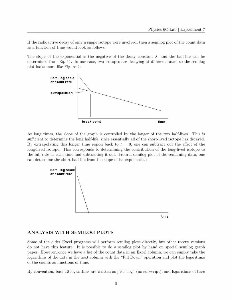
If the radioactive decay of only a single isotope were involved, then a semilog plot of the count dataas a function of time would look as follows:

The slope of the exponential is the negative of the decay constant λ, and the half-life can bedetermined from Eq. 11. In our case, two isotopes are decaying at different rates, so the semilogplot looks more like Figure 2:

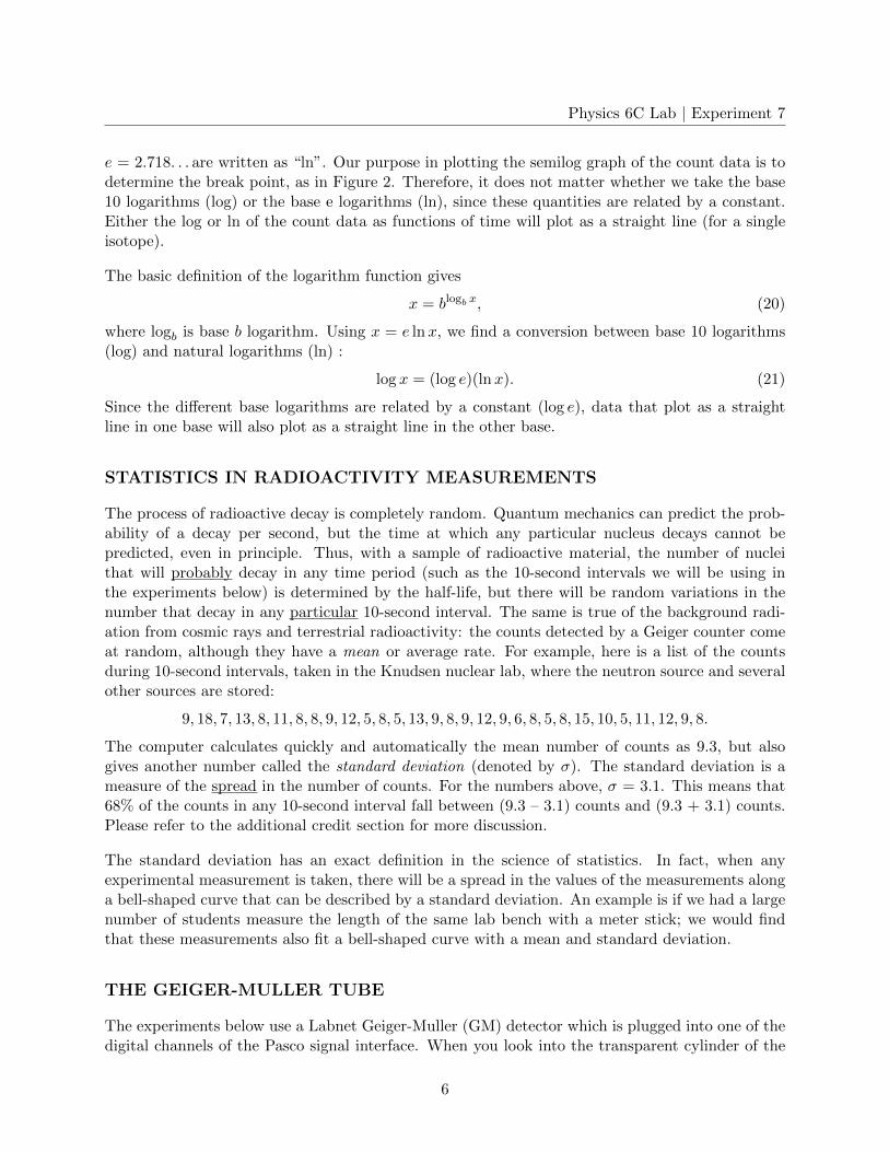
At long times, the slope of the graph is controlled by the longer of the two half-lives. This issufficient to determine the long half-life, since essentially all of the short-lived isotope has decayed.By extrapolating this longer time region back to t = 0, one can subtract out the effect of thelong-lived isotope. This corresponds to determining the contribution of the long-lived isotope tothe full rate at each time and subtracting it out. From a semilog plot of the remaining data, onecan determine the short half-life from the slope of its exponential:

ANALYSIS WITH SEMILOG PLOTS

Some of the older Excel programs will perform semilog plots directly, but other recent versionsdo not have this feature. It is possible to do a semilog plot by hand on special semilog graphpaper. However, once we have a list of the count data in an Excel column, we can simply take thelogarithms of the data in the next column with the “Fill Down” operation and plot the logarithmsof the counts as functions of time.

By convention, base 10 logarithms are written as just “log” (no subscript), and logarithms of base

5


e = 2.718. . . are written as “ln”. Our purpose in plotting the semilog graph of the count data is todetermine the break point, as in Figure 2. Therefore, it does not matter whether we take the base10 logarithms (log) or the base e logarithms (ln), since these quantities are related by a constant.Either the log or ln of the count data as functions of time will plot as a straight line (for a singleisotope).

The basic definition of the logarithm function gives

x = blogb x, (20)

where logb is base b logarithm. Using x = e lnx, we find a conversion between base 10 logarithms(log) and natural logarithms (ln) :

log x = (log e)(lnx). (21)

Since the different base logarithms are related by a constant (log e), data that plot as a straightline in one base will also plot as a straight line in the other base.

STATISTICS IN RADIOACTIVITY MEASUREMENTS

The process of radioactive decay is completely random. Quantum mechanics can predict the prob-ability of a decay per second, but the time at which any particular nucleus decays cannot bepredicted, even in principle. Thus, with a sample of radioactive material, the number of nucleithat will probably decay in any time period (such as the 10-second intervals we will be using inthe experiments below) is determined by the half-life, but there will be random variations in thenumber that decay in any particular 10-second interval. The same is true of the background radi-ation from cosmic rays and terrestrial radioactivity: the counts detected by a Geiger counter comeat random, although they have a mean or average rate. For example, here is a list of the countsduring 10-second intervals, taken in the Knudsen nuclear lab, where the neutron source and severalother sources are stored:

9, 18, 7, 13, 8, 11, 8, 8, 9, 12, 5, 8, 5, 13, 9, 8, 9, 12, 9, 6, 8, 5, 8, 15, 10, 5, 11, 12, 9, 8.

The computer calculates quickly and automatically the mean number of counts as 9.3, but alsogives another number called the standard deviation (denoted by σ). The standard deviation is ameasure of the spread in the number of counts. For the numbers above, σ = 3.1. This means that68% of the counts in any 10-second interval fall between (9.3 – 3.1) counts and (9.3 + 3.1) counts.Please refer to the additional credit section for more discussion.

The standard deviation has an exact definition in the science of statistics. In fact, when anyexperimental measurement is taken, there will be a spread in the values of the measurements alonga bell-shaped curve that can be described by a standard deviation. An example is if we had a largenumber of students measure the length of the same lab bench with a meter stick; we would findthat these measurements also fit a bell-shaped curve with a mean and standard deviation.

THE GEIGER-MULLER TUBE

The experiments below use a Labnet Geiger-Muller (GM) detector which is plugged into one of thedigital channels of the Pasco signal interface. When you look into the transparent cylinder of the

6


detector, the actual GM tube is the copper cylinder at the bottom end, which appears similar to alarge bullet cartridge. The rest of the electronics inside the transparent tube consists of the powersupply for the GM tube which operates at 300 – 400 V DC, and the digital interface that amplifiesthe GM pulses and converts them to digital pulses accepted by the signal interface box.

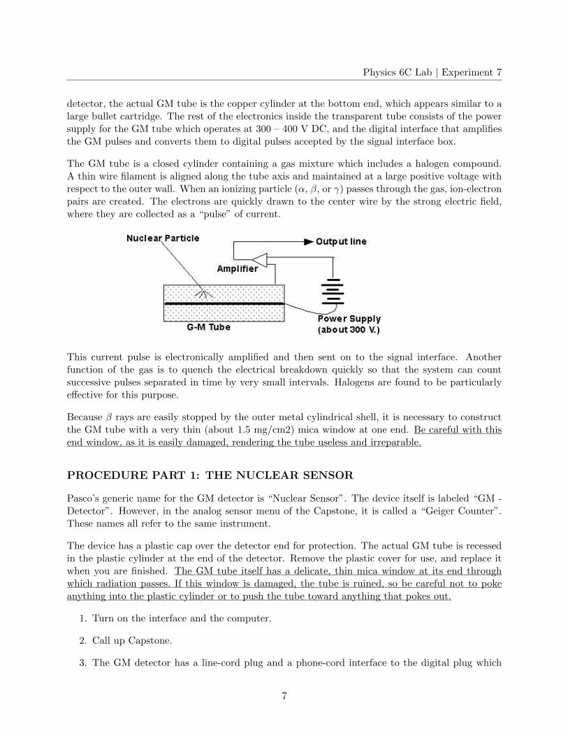
The GM tube is a closed cylinder containing a gas mixture which includes a halogen compound.A thin wire filament is aligned along the tube axis and maintained at a large positive voltage withrespect to the outer wall. When an ionizing particle (α, β, or γ) passes through the gas, ion-electronpairs are created. The electrons are quickly drawn to the center wire by the strong electric field,where they are collected as a “pulse” of current.

This current pulse is electronically amplified and then sent on to the signal interface. Anotherfunction of the gas is to quench the electrical breakdown quickly so that the system can countsuccessive pulses separated in time by very small intervals. Halogens are found to be particularlyeffective for this purpose.

Because β rays are easily stopped by the outer metal cylindrical shell, it is necessary to constructthe GM tube with a very thin (about 1.5 mg/cm2) mica window at one end. Be careful with thisend window, as it is easily damaged, rendering the tube useless and irreparable.

PROCEDURE PART 1: THE NUCLEAR SENSOR

Pasco’s generic name for the GM detector is “Nuclear Sensor”. The device itself is labeled “GM -Detector”. However, in the analog sensor menu of the Capstone, it is called a “Geiger Counter”.These names all refer to the same instrument.

The device has a plastic cap over the detector end for protection. The actual GM tube is recessedin the plastic cylinder at the end of the detector. Remove the plastic cover for use, and replace itwhen you are finished. The GM tube itself has a delicate, thin mica window at its end throughwhich radiation passes. If this window is damaged, the tube is ruined, so be careful not to pokeanything into the plastic cylinder or to push the tube toward anything that pokes out.

1. Turn on the interface and the computer.

2. Call up Capstone.

3. The GM detector has a line-cord plug and a phone-cord interface to the digital plug which

7


goes into the signal interface. When the line cord of the GM detector is plugged in, a neonbulb inside lights up, indicating that the instrument has power. The other neon bulb flashesintermittently as each count is detected. This happens whether or not you are recording ormonitoring and even if there are no radioactive materials nearby, because the tube detectsstray cosmic rays and terrestrial radioactivity that are always present.

4. Choose the “Table & Graph” option in Capstone. Under “Hardware Setup”, click on Channel1 of the interface and select “Geiger Counter”. At the bottom of the screen, change the sampletime to 10 seconds. This will give you one measurement every 10 seconds of recording time.Click on the y-axis of the graph and select “Geiger Counts (counts/sample)”. Click on “SelectMeasurement” in your table and choose “Geiger Counts (counts/sample)”. If your watch hasa continuously illuminated night dial, it may contain a small amount of radioactive material.Check the watch with the detector if you wish, and take it off and move it some distanceaway if you find that it is radioactive.

5. Move all radioactive materials at least one meter from the detector and take a backgroundcount by clicking “Record” and counting for 100 – 120 seconds. Then click “Stop”. Yourtable should now have approximately 10 entries for the count every 10 seconds.

6. When you click the∑

symbol on the table, the computer will calculate the mean count andstandard deviation below (along with the minimum and maximum count). Record the meanbackground count and its standard deviation. Your count will be higher than “normal” ifyour lab station is close to the neutron source used in the half-life measurement below.

Background count (mean) =

Standard deviation =

PROCEDURE PART 2: HALF-LIFE MEASUREMENTS

(The instructions for Excel are abbreviated, as it is assumed that you are familiar with the opera-tions.)

1. Check that you are counting for 10-second intervals. Prepare your computer to start takingcount data on the next mouse click by setting the mouse arrow on the “Record” button.

2. When you are ready, the radiation safety officer will hand you a rod with the activated silverfoil on the end. As quickly as possible, but still being careful, place the rod in the holder withthe silver close to the GM counter, and click to start recording. Stop after approximately 10minutes.

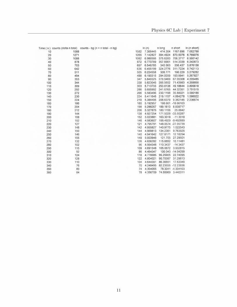
3. Copy the silver count data from your table into a column of a new Excel worksheet.

4. Subtract out the background count in the next column of the worksheet.

5. Use the “Fill Series” operation to fill the next column of the worksheet with the time of thecenter of the 10-second intervals (i.e., 5, 15, 25, etc.), up to 10 minutes.

8


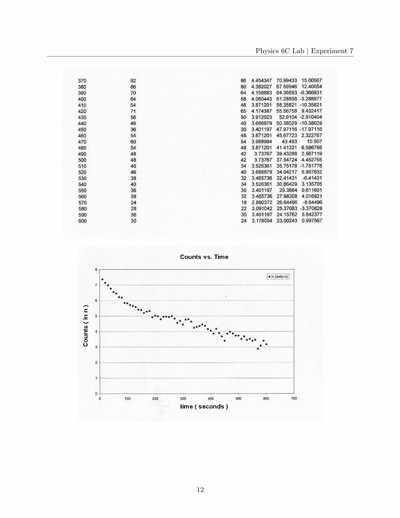
6. Use the “Fill Down” operation to take the logs or lns of the count data (it doesn’t matterwhich) in the next column.

7. Chart the logs of the data as functions of time. (Select and chart the last two columns.) Thissemilog chart should look something like Figure 2: a straight line of steeper slope breakingto a line of shallower slope, corresponding to the two half-lives involved. The data at largetimes is likely to look ragged due to fluctuations in the statistics. We now wish to extractthe two half-lives.

8. Locate the break point in time where the slope changes at about 150 seconds.

Break point =

9. Back in Excel, select and chart only count data after the break point. (Chart the actualdata, not their logs.) Select the data points on the chart, and use the trendline operationto fit an exponential curve. Check the box for “Equation on Chart” to obtain the slope ofthe exponential. From this slope, extract the longer half-life using Eq. 11, and record thishalf-life below.

Longer half-life =

10. To obtain the shorter half-life, start a new column in Excel, and subtract from the background-corrected data, the data for the longer half-life using the equation that you obtained in step10. (Your entry before “Fill Down” will look something like ”= C4 - 609*exp(-0.0035*B4)”.)

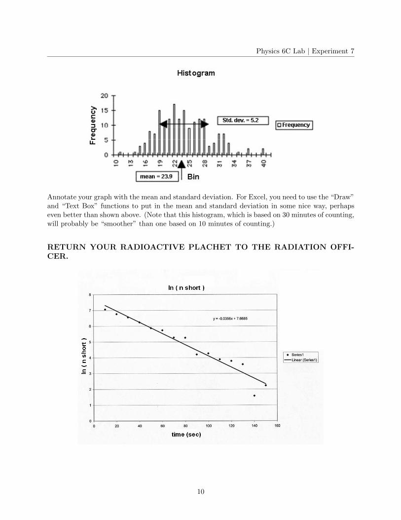
11. Chart the resulting data, and extract the shorter half-life as before with the trendline opera-tion.

Shorter half-life =

12. Rearrange your Excel tables and charts neatly on one or two sheets.

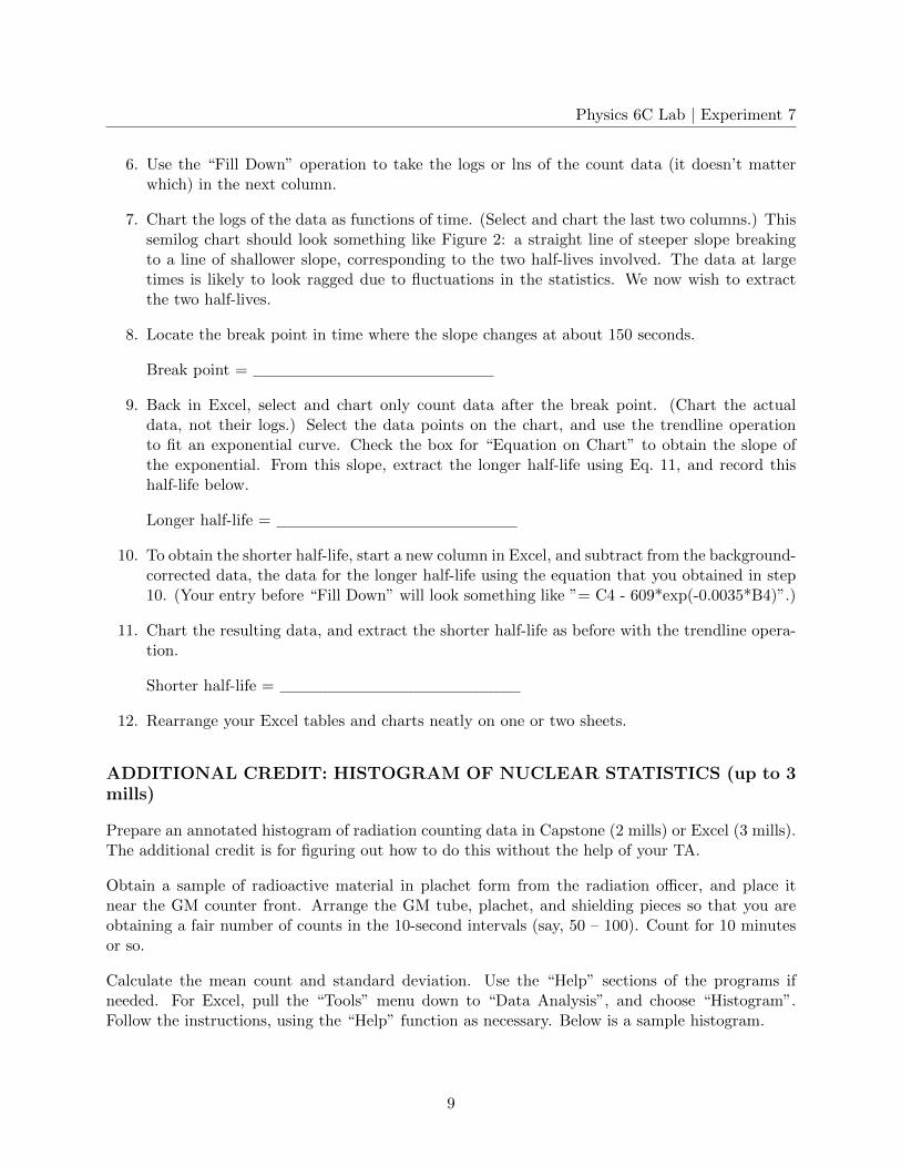
ADDITIONAL CREDIT: HISTOGRAM OF NUCLEAR STATISTICS (up to 3mills)

Prepare an annotated histogram of radiation counting data in Capstone (2 mills) or Excel (3 mills).The additional credit is for figuring out how to do this without the help of your TA.

Obtain a sample of radioactive material in plachet form from the radiation officer, and place itnear the GM counter front. Arrange the GM tube, plachet, and shielding pieces so that you areobtaining a fair number of counts in the 10-second intervals (say, 50 – 100). Count for 10 minutesor so.

Calculate the mean count and standard deviation. Use the “Help” sections of the programs ifneeded. For Excel, pull the “Tools” menu down to “Data Analysis”, and choose “Histogram”.Follow the instructions, using the “Help” function as necessary. Below is a sample histogram.

9


Annotate your graph with the mean and standard deviation. For Excel, you need to use the “Draw”and “Text Box” functions to put in the mean and standard deviation in some nice way, perhapseven better than shown above. (Note that this histogram, which is based on 30 minutes of counting,will probably be “smoother” than one based on 10 minutes of counting.)

RETURN YOUR RADIOACTIVE PLACHET TO THE RADIATION OFFI-CER.

10


11


12

physics 6c lab experiment 7...

Documents