PHY111: General Physics I

Laboratory Manual

Student’s Edition

Spelman College Fall 2007

2

Table of Contents General Information.........................................................................................................................3 Introduction..........................................................................................................................3 General Policies ...................................................................................................................4 Format of Lab Report...........................................................................................................7 Uncertainty and Errors.........................................................................................................8 Graphing ............................................................................................................................12 Computer Spreadsheet ………………………………………………………………….. 14 Experiment #1: Introduction to Procedures and Measurements...................................................15 Experiment #2: Free-Fall Motion and Projectiles.........................................................................17 Experiment #3: Vectors ................................................................................................................19 Experiment #4: Kinematics...........................................................................................................21 Experiment #5: Newton's Second Law.........................................................................................23 Experiment #6: Forces--Springs and Buoyancy ...........................................................................26 Experiment #7: Prosthetic Arm ....................................................................................................29 Experiment #8: Work and Energy ................................................................................................31 Experiment #9: Work and Thermal Energy..................................................................................33 Experiment #10: Thermal Energy and Phase Changes.................................................................35 Experiment #11: Momentum, Collisions, and Mass.....................................................................37 Experiment #12: Design of an Experiment...................................................................................39

3

General Information Introduction Controlled experiments form the basis for our belief in the physics theories that you find in your textbooks. Ultimately, experiments and observations provide a final test that any theory must pass to be accepted by scientists. The experiments in this course use relatively simple equipment and deal with well-established physics. By performing these experiments, however, you will learn how physicists apply the scientific process by measuring physical quantities (such as distance and time) and by discovering mathematical relations between these quantities. Most importantly, you will learn to develop ideas about how the physical world behaves and to plan, carry out, and analyze experiments to test those ideas. You should not treat this manual as a cookbook, but rather as a guidebook. In some cases, you may decide to modify the given procedure (within the limitations of available equipment). In other cases, you may go beyond the given procedure. In a few cases, you must create your own procedure from scratch. In any case, you should understand the purpose of the procedure and how the procedure fulfills that purpose.

4

General Policies Safety You must conduct yourself in a safe manner at all times in the laboratory. Exercise caution in everything that you do. Report injuries, no matter how minor, immediately to the instructor. Examples of safe conduct are listed below:

• Do not lift heavy equipment without assistance. • Do not reach for supplies on high shelves without the use of a stepstool and

assistance. • Handle all equipment with care; make sure that you understand the proper use and

limitations of all equipment. When in doubt, ask the instructor. • Do not allow laser light to go into your eyes. Do not position a laser so that its

light may go directly or reflect into someone’s eyes. • Be aware of a first-aid kit and fire extinguisher during the first lab period.

Consult your instructor if you cannot locate these. • Do not put anything in your mouth or use your mouth to handle anything. • Dispose of materials properly, including chemicals and radioactive materials.

Your instructor will inform you about disposal or handling procedures, if necessary.

This list is not complete, but you should get the idea that safety is a serious issue and you must conduct yourself accordingly. Your instructor will review safety features of the laboratory and other safety issues with the class during the first period. Computers During the lab period, do not use the computers for work not related to the lab. If you do so, then your grade may be affected (see policy on grading). However, you may use the computers outside of class with the permission of the instructor, lab coordinator, or other authorized physics department personnel. Use your Spelman student login to access the computers. If you do not have a user id and password, speak with the instructor. Please logout when you are finished with the computer; do not shut down the computer. Do not save anything on the computer, since it will be automatically erased within one day. Save your work on a flash drive instead. Do not change any computer settings or download anything, even if you know that it is safe.

5

Grading Remember that you must pass the laboratory portion of the course (60% or greater) to receive a passing grade for the course, even if you score 100% in other components of the course. You will not receive a separate lab grade; your course grade will include your laboratory work. Group Leader 100 points per session Lab participation 25 points per session Lab reports 100 points each The instructor will assign a group leader each week and it will rotate among the group members. The group leader will be graded on the following responsibilities: 1) whether the work is distributed among group members fairly and efficiently, and everyone is actively engaged; and 2) whether the work is done properly with scientific merit. In addition, only the group leader will be allowed to communicate with the instructor concerning the lab activities. However, the instructor may interact with any group member. The group leader will evaluate each group member so that the instructor can assign lab participation points. Your grade is computed by dividing your total earned points by the total possible points. If you get less than 60% on the lab grade, you will receive a grade of F for the entire course, regardless of your exam grades. The lab grade counts 20% of the course grade; consult your syllabus. Required Materials You must bring a scientific calculator, a ruler, and a protractor to lab. Preparation You should come prepared to the laboratory session by reading the lab manual ahead of time. Note all questions and areas of confusion which can be brought up in group discussions in the lab. You should also review any appropriate sections of the textbook. Your preparation should also include coming to lab with all accessories (calculator, rules, notebook, protractor, writing utensil, etc.). If you are the group leader for that week, you should have a preliminary plan of the work and be ready to discuss the work with the instructor and group members. Absences and Tardiness

6

If you arrive late for lab, your lab participation grade will be reduced. If you are more than 15 minutes late or miss lab, you will not be allowed to join your group or make-up the lab unless you have made previous arrangements with your instructor or you have a legitimate excuse as determined by the instructor. Without previous arrangements or a legitimate excuse, you will receive a zero for that week’s lab. If you are late or miss any make-up session, you will not be allowed to make-up the lab and will receive a grade of zero for that lab. Academic Honesty You should work together with your lab partners in taking and analyzing data, and you will find that discussing the experiment with your partners helps you to understand the results. However, you should record your own data, and the lab reports that you turn in must be your own work in your own words. You cannot copy or paraphrase your partner's reports. Please refer to the section on Academic Dishonesty in the college's student handbook. Lab Reports The grade on the lab reports will constitute the bulk of your lab grade. The format of the lab report is summarized below. Your instructor may only require certain parts of the lab report for a particular week or may require a complete lab report. Before you leave lab, you must record your data and obtain the instructor's signature on your data sheet. This sheet must be included in your report, so you should record your data neatly in lab. If you have time remaining in lab, you should work on your graphs and calculations. You should not leave early unless you have finished your report. Lab reports are due one week after you perform the experiment at the beginning of the lab period. You will be deducted 20% per school day or part of a school day for late lab report. Therefore, you should start working on your reports early in the week; this allows you time to seek help if you are having trouble. Writing Style Your lab reports should be clearly written and easy to follow. Use complete sentences and coherent paragraphs. Points may be taken off for poor writing. If you are having trouble, please see the instructor or go to the Writing Center for help.

7

Format of Lab Report Basic Information

• Title of experiment • Your name and the names of your lab partners • Date of experiment • Purpose of experiment

Data

• Summary of procedure – only include procedure not detailed in lab manual or if you make changes in the procedure

• Original data neatly recorded as measured, including units • Tables often provide a good format for recording data; see below for a sample data

table • Estimated uncertainties of measurements (random error) • Possible sources of error, particularly systematic error

Calculations and Results

• Sample calculation for each type of calculation Include the formula used, then put sample numbers into the formula and

show the calculation Include units in sample; convert units as needed

• Collection of results of calculations (possibly in a table) • Estimation of uncertainties • Graphs

Discussion and Conclusions

• Summarize results, focusing on the stated purpose of the lab • Discuss the consistency of your results with previous or accepted results, or with

theory • Discuss the significance of your result • Suggest improvements to the experiment, particularly to reduce sources of error

(random or systematic) • Answer any questions in the manual

Each sub-section above will be assigned points each week for a total of 100 points. The number of points per sub-section may change from week to week.

8

Uncertainty and Errors No experiment is perfect. Certainly, you should perform your experiments carefully and use good equipment. When you make a measurement, however, you should consider the possible sources of error in that measurement. When you report the measurement, you must also report an estimate of the error of that measurement. Random Errors, Precision, and Uncertainty If you measure the length of a room twice, you will probably find that the two measurements differ. This results from limits on the precision of measurements. A more precise measurement is one that, when repeated, tends to yield nearly the same number. Two factors limit the precision of measurements. First, when you measure the length of the room, you might not place the meter stick exactly the same way each time. This introduces random error into the measurement. Second, the markings on a meter stick are separated by one millimeter. If the end of the room lies between two markings, you must estimate the length between the markings. This type of random error is inherent in any measuring device. In both of these cases, the measurement has a random error that limits the precision. Suppose that you measure the motion of a car, using a stopwatch to keep track of time and looking at marks on the road to determine the position of the car every 10 seconds. Suppose that the marks are 20 m apart. Then, you could accurately see whether the position is 20 m rather than 40 m, but you could not accurately see whether the position is 25 m rather than 27 m. You can, however, estimate the position as 25 m and state the uncertainty of your measurement. If you are confident that the position is between 20 m and 30 m, then the uncertainty is 5 m on either side of 25 m. Thus, you would record the measurement as 25 m ± 5 m. The uncertainty of 5 m represents your estimate of the random error. Note that, in recording a measurement, the last digit is estimated; always estimate one digit past the digits that you can determine exactly. In other words, the last digit that you write down is the first uncertain digit. For most instruments in this course, you must gauge the amount of uncertainty yourself. A good rule of thumb is that the uncertainty is one-half of the smallest division on the scale. In our example, this gives an uncertainty of 10 m. In some cases, you may judge that your uncertainty is larger or smaller. In our example, for instance, you probably can actually judge the position to within 5 m rather than within 10 m. If you are reading an electrical meter, you would record a larger uncertainty if the numbers are fluctuating than if the numbers are steady. In any case, your data must include the uncertainty of all measurements and justification for the numbers that you record for uncertainty. Also, you should note the possible sources of random error. Finally, in your discussion and conclusion you should suggest ways of reducing or eliminating those sources of error.

9

Averages and Deviations You can minimize the effect of random errors by making several independent measurements and averaging those measurements. Then, the random errors will cancel out during the averaging. For instance, suppose you made several measurements of the time for a ball to fall from your dorm window to the ground: Trial Time (s); ±0.05 s 1 2.15 2 2.25 3 2.35

Averages s s

s = + +

= .2.15 2.25 2.35

32.25

Because the times are different for the different trials, you cannot have perfect confidence in the average. To calculate the uncertainty of the average, you can calculate how much each measurement differed from the average (deviation), then average the absolute values of the deviation. Trial Time (s) Absolute Value of Deviation 1 2.15 2.15 s − 2.25 s = 0.10 s 2 2.25 2.25 s − 2.25 s = 0.0 s 3 2.35 2.35 s − 2.25 s = 0.10 s

Average deviation = 010 0 00 010

3. . .s s s+ +

= 0.07 s.

The average deviation is bigger than the uncertainty in the individual data points, so the deviation controls the uncertainty. You then report your result as 2.25 s ± 0.07 s. Consistency When you compare your results with other results or to a theory, you must consider your uncertainty. For example, suppose you measure the mass of a ball as 1.55 ± 0.05 kg. That is, you believe that the mass is between 1.50 kg and 1.60 kg. If another student measures the mass as 1.50±0.05 kg (that is, between 1.45 kg and 1.55 kg), then the range of her measurement overlaps with the range of your measurement. Therefore, her result is consistent with your result. If her measurement is 1.10±0.05 kg, however, then her range does not overlap with your range, and so her result is not consistent with your result.

10

Combining Uncertainties Sometimes, you will make calculations involving two or more measurements that have uncertainty. For example, suppose that you have calculated a speed as

with an uncertainty of 5 m in distance and 1 s in time. Then, the largest speed consistent with your data would be (55 m)/(4 s) = 14 m/s, and the uncertainty would be 4 m/s. You should make sure that you understand why the numbers 55 m and 4 s were used in this example. (Remember that you want to find the largest speed consistent with your data.) Systematic Errors and Accuracy Suppose that your stopwatch runs slow. Then, all of your measured times would be too small by some constant factor. In other words, your measurements would have a systematic error. As another example, suppose that you have a properly-running stopwatch, but you started it one second too late at the beginning. Then, all time measurements would be one second too small, producing a type of systematic error known as zero error. Even if your measurements have very small random error, the systematic error would reduce the accuracy of your measurements. You cannot reduce systematic errors by repeated measurements and averaging. You can, however, eliminate systematic errors through use of carefully calibrated equipment and proper procedure. For instance, you could check your stopwatch against an atomic clock. In practice, you may not have the opportunity to fully calibrate your equipment in this class. As you take data, however, you should take note of possible sources of systematic error (include in your report in the Data section). If you can measure the systematic error, then you can make corrections during your calculations. For instance, if your stopwatch consistently started running 0.1 s after you pushed the button, you could add 0.1 s to your times when you do your calculations. Do not, however, make these corrections before you record your measured times; record the data as the stopwatch actually reads, then make the corrections later.

speed distancetime

ms

m s = = = / ,505

10

11

Graphing You will often measure one quantity while varying another quantity. In a moving car example, you can measure position as time change. In the lab, you could record these data in a table. Physics does not consist, however, simply of data tables; physicists try to find mathematical relationships between measured quantities. To find an equation for how position depends on time, you could plot position versus time in a graph. Then, you could tell whether position is proportional to time (straight line) or whether the relationship is more complicated (curve). Physically, your graph would tell you whether the car was moving at constant speed or accelerating. The graph below is for position versus time. In this case, the position was measured at specific times. Generally, the variable that you set or control appears on the horizontal axis, while the variable that you measure appears on the vertical axis. Had you measured the times at which the car crossed specific positions, then you would graph time versus position.

position = 30.445 time + 172.66

0

500

1000

1500

2000

2500

3000

0 20 40 60 80 100

time (s)

posi

tion

(m)

Analysis of Straight Lines If your data fall on a straight line, then you should calculate the slope of that line. The line is drawn as close to the data points as possible. Usually, the slope is an interesting physical quantity. In the sample graph, the slope is labeled as displacement divided by time, or labeled as the velocity of the car. To calculate the slope of a straight line, choose two points on the line and mark them. Do not simply use two of your data points to calculate the slope, since then you would throw

12

away the rest of your data. For the sample graph, the slope is calculated using the points (5 s, 325 m) and (60 s, 2000 m):

Since the data points do not all lie on the line, you cannot be certain about the slope. To compute the uncertainty of the slope, draw two lines parallel to the best line and two other lines perpendicular to it. A box drawn should contain about two-thirds of the data points. Then, the diagonals of the box represent the second-best lines to describe the data. Calculate their slopes; then, one-half of the difference between these second-best slopes is the uncertainty in the slope:

In this case, you would quote your result as 30 m/s ± 10 m/s. (Actually, it would be best to write this in scientific notation, with one digit.) Analysis of Curves Sometimes, your data points will not lie on a straight line. Usually, you will then try to draw another graph that does have a straight line. For instance, if you see the curve drawn to the side (which looks like a square-root function), then you might try to draw a graph of y2 versus x. If the new graph is a straight line, then you can conclude that the original graph is described by a square-root function. Using the slope of the new graph, you can determine the precise mathematical relation between x and y. Another analytical method is to graph changes in measured quantities. For instance, instead of graphing position as shown, you could graph the change in position during each time interval. You can often use a hypothesis as a guide in analyzing data. If you believe that the car in the sample graph has cruise control, then you might suspect that speed is constant and that the change in position is the same for all time intervals. This line of reasoning would suggest that you calculate the change in position.

.sm4.30

s5s60m325m2000

timeof changeposition of change =

- = −

12

(34.1m / s - 14.3m / s) = 9.9 m / s .

x

y

13

Computer Spreadsheets You can use Excel to help you make graphs and fit lines to data points. See the

document Excel Instructions for Physics Lab. This document contains the features of Excel that is relevant to this course. They include writing a formula for calculations and graphing.

14

Experiment #1: Introduction to Procedure and Measurements

Goals The goals are more than the “purpose of the experiment”, which indicates a scientific reason for the experiment. For instance, the purpose of this experiment involves a geometric quantity which relates to the nature of space. The goals, however, also include skills that you should learn and attitudes that you should develop while doing the experiment. In this experiment, the goals include recording data with uncertainty, calculating averages and deviations, and propagating uncertainty. Background In Euclidean geometry, the ratio of the circumference of a circle to its diameter is shown to be a constant, π. According to modern theories about the structure of space, Euclidean geometry might not describe the universe on a large scale. Then, the ratio of circumference to diameter would not be π. If you measure two quantities, their relationship may be determined by plotting one against the other. If a straight line that passes through the origin describes the data, then the ratio of the quantities is a constant given by the slope. You must read the General Information section of the lab manual before this lab session. Your lab instructor will not lecture you on this material, but you will use it during the experiment. Exercise Use 5 circular objects and plot the circumference versus the diameter. Measure these quantities several times so that you can estimate the random uncertainty by the average deviation. Indicate the uncertainty on the plot by using error bars. Discuss with your group to determine the best way to measure the circumference. Use a vernier caliper to measure the diameter for small enough objects. Your instructor will tell you how to use this instrument. Record all possible sources of random uncertainty. If the data indicates that the relationship of circumference to diameter can be described by a straight line, use Excel to determine the equation of the best-fit straight line to the data, along with uncertainties on the slope and intercept. See instructions on how to do this in the document Excel Instructions for Physics Lab located on the physics web page. Report For this experiment, you will turn in a paragraph on the scientific purpose(s) of the experiment, data organized clearly in table(s), sample calculations, your graph, a table of results with uncertainty, and a discussion. Your discussion must include your conclusion in regards to your scientific purpose(s), how you arrived at your conclusions based on your data and results, an interpretation of the results based on your expectations, and comments on ways to improve the experiment if you were able to repeat it.

15

Somewhere in your report you must address the following questions: 1) What is the relationship between circumference and diameter? 2) Is a straight line a good fit to the data points? Explain. (The words “error bars”

should occur in your explanation.) 3) Does the value of the slope make sense? the intercept? 4) Based on the results from your experiment, what do you predict the diameter of the

earth to be (along with uncertainty) from the know circumference of 24,902 miles? 5) Is Euclidean geometry valid for the objects used in the experiment? Your report will be graded as follows:

• Data (complete, proper instrumental uncertainties, clear and organized; include a description of your technique to measure circumference) - 30 points

• Data Analysis/Results (proper calculations, graph, and fitting procedure; uncertainty in slope and intercept; proper reporting of uncertainty as average deviation or instrumental uncertainty) – 40 points

• Scientific Purpose/Results/Discussion/Questions (scientific purpose, results, experiment, conclusions are all appropriately connected and stated; reasonable statement about improving experiment; answers to questions accurate and complete) – 30 points

16

Experiment #2: Free-Fall Motion and Projectiles

Goals This experiment will help you discern the relationship between position and velocity, as well as the relationship between velocity and acceleration. You will also examine how these relationships apply to free-fall in one dimension and in two dimensions. In addition, you will learn to use a computer spreadsheet to analyze and graph your data. This will be a two-week experiment. If you are not familiar with computer spreadsheets, you should do your first spreadsheet analysis in lab. See Excel Instructions for Physics Lab. Background According to the ancient Greeks, objects fall at different speeds depending on their masses. Galileo's experiments, however, showed that objects fall with constant acceleration, independent of mass, if air resistance does not play a significant role. The instantaneous velocity at time t1 can be estimated as the average velocity between times t1 and t2, provided that the time interval is small. Exercise Use a webcam to record a video of a free-falling object after it is thrown straight up and until it comes down. See the document Webcam Instructions for Physics Lab. Import your video into Logger Pro and obtain data for the y-position of the object versus time (ignore x, even though the software gives both x and y). See the document Lab Pro and Logger Pro. Save the data as a text file and import it into Excel. Use Excel to graph the y-position of the ball versus time. See the document Excel Instructions for Physics Lab. In the Discussion section of your report, you should comment on your graph: What does it say about the motion of the ball? Estimate the uncertainties in the position coordinates and the time (you estimate uncertainties when you do not repeat the measurements, rather that using average deviation as in the previous experiment). In your report, you should explain how you came up with your uncertainty estimates. Your data points probably did not fall on a straight line. What quantity could you calculate that would give a straight line when plotted versus time? After you reach a consensus in your group, discuss your choice with your instructor. In the Discussion section of your report, you should justify your choice and explain the physical meaning of the calculated quantity. Since the new graph requires some calculations, remember to show a sample calculation in your report (including units). Propagate the uncertainties on the position and time to the uncertainty on the calculated value using the max/min method (see the introductory material in the manual). You can use Excel to perform the actual calculations. Make the new graph (including error bars) and draw a straight line through the points. (If the points do not fall on a straight line, then you need to make a different graph.) Use Excel to fit a straight line to the data and to calculate the slope. Use Excel to also determine the uncertainties in the slope and intercept. In your Discussion, discuss whether your results agree with Galileo or not. Also discuss possible sources of

17

error, particularly systematic error, and ways of dealing with those errors if you did the experiment again. Repeat the above for a different object thrown as a projectile in two-dimensions. In this case, perform the measurements and data analysis on both x and y coordinates. Make sure that your video captures the range of the horizontal motion. Report Your report will consist of a statement about the purpose(s) of the experiment, data, data analysis, and a discussion. The data must include graphs of the position versus time for both the one- and two-dimensional motions, along with uncertainties (note that in reporting data as a graph, you only report the data points and error bars; you do not connect the data points). The data analysis consists of calculating and graphing the quantity (along with uncertainty) that will generate a straight line and obtaining the equation of the straight line with uncertainties in the slope and intercept – do the data analysis separately for both the one- and two- dimensional motions. Your discussion should include all the points mentioned in the Exercise section, as well as an interpretation of the slopes and intercepts. In addition, include in your discussion a comparison of the one- and two-dimensional motions; mention all similarities and differences. The grading is as follows: Data (complete, clear, proper graph) – 20 points; data analysis/results – 40 points; purpose/results/discussion – 40 points.

18

Experiment #3: Vectors

Goals The main goal is to better acquaint you with vectors. In particular, you will determine whether force is a vector quantity, by investigating how forces add. You will, therefore, also practice vector addition. Finally, you will continue to learn about comparing numbers and about uncertainty. Background We may define a vector quantity as any quantity that adds in the same way that displacements add, and a scalar quantity as any quantity that adds like ordinary numbers. If a physical quantity is a vector, then we may represent it on paper as a displacement arrow with a particular length and direction. There must be some scale that converts from the length on the paper to the magnitude of the vector, and there must be a particular coordinate system for measuring angle. Alternatively, we may represent a vector in terms of its components along the x and y directions. To add vectors pictorially, draw the first vector with the appropriate length (according to the scale) and direction. Then, draw the second vector with its tail located at the tip of the first vector. The second vector must have the correct direction relative to the coordinate system, not relative to the first vector. Continue this process with all vectors. The sum is then drawn from the tail of the first vector to the tip of the final vector. The sum will have uncertainty, based on your ability to measure its length and direction. A force table is a metal disk with angles marked on the edge. Strings are attached to a ring at the center of the table. The strings run over pulleys attached at the edge (at a particular angle), with weights on the ends of the strings. Therefore, one may apply controlled forces at chosen directions, acting on the central ring. If the forces add to zero, then the ring will not move; this condition is known as equilibrium. Exercise Discuss with your group and make up the magnitudes and directions of two forces; the magnitudes should be between 100 and 200 units and the directions should be chosen so that they are not perpendicular to each other. You will now proceed to add these forces using three different methods. First, as a group, use the force table to determine the sum of the two chosen forces. The magnitudes of the forces are represented by the masses attached to the strings (not entirely correct since the mass and the force due to the weight of the mass are not the same, but since they are proportional on earth, we will ignore the difference for this experiment). Set up strings on the force table for the two made-up forces at the appropriate directions. Hang masses to represent the magnitudes of the forces. Experimentally find the third force necessary for the ring to be in equilibrium; determine both magnitude and direction of the third force. To estimate uncertainty on the magnitude and direction of the third force, find the range of angle and of mass that will keep the ring

19

in equilibrium. You can do this by establishing equilibrium, then making small changes until equilibrium is lost. The largest change that maintains equilibrium is an estimate of your uncertainty. Since the three forces add to zero, then the sum of your original two forces is the negative of the experimentally found third force. You should now have the magnitude and direction of the sum of your original forces with uncertainties. The second method is to add the made-up forces using arrows drawn to scale; do this individually. Choose a scale and a coordinate system so that the arrows representing these forces will fit on the paper. Representing these forces pictorially, find the magnitude and direction of the sum of your original two forces. The uncertainties may be estimated from the uncertainty in reading the ruler (converted using the scale) and protractor. You may add a little to the estimated uncertainties to account for small errors in drawing the arrows. You should now have the sum of your original forces a second time, along with uncertainties in the magnitude and direction. Use vector components as a third method of finding the sum of your original two made-up forces; do this individually. Use trigonometric and algebraic equations to find the components of the sum. Then, determine the magnitude and direction of the sum. This is a purely mathematical method, so there is no uncertainty in the result. Report Your report must consist of force table data and sum of the original two forces with uncertainties in the magnitude and direction, your pictorial addition with stated scale and the result of the sum with uncertainties, the component addition, discussion, and answer to questions below. Each part is worth 20 points. The discussion must include a comparison of the results of the three methods and appropriate conclusions about the vector nature of forces. It must also include a discussion about agreement or disagreement of the results of the three methods. Questions: 1. Classify each of the three methods as experimental or theoretical, and explain the

reason(s) for your classification. 2. How do today’s activities exhibit the scientific process? 3. Design an activity to test whether velocity is a vector quantity.

20

Experiment #4: Kinematics

Goals This experiment will help you discern the relationship between position and velocity, as well as the relationship between velocity and acceleration. You will also learn to use an ultrasonic motion detector that is interfaced to a computer to analyze motion in one dimension. Finally, you will study motion on an inclined low-friction plane. Background In this experiment, you will use a motion detector interfaced to a computer to study motion. On the Physics Department webpage, click on Lab Manuals --> Logger Pro and Lab Pro to find instructions on the use of the Lab Pro interface box, the motion detector, and the Logger Pro software. Set up and become familiar with the equipment before proceeding to the exercise. You should also become familiar with selecting a portion of a graph produced by Logger Pro and fitting it to a straight line (if applicable) in Logger Pro. Exercise Velocity Set up the software for plots of position and velocity. Pushing the cart by hand, achieve a constant positive velocity. Describe how you moved the cart (for instance, towards or away from the detector, with a steady or a changing push). Discuss the relation between the position plot and the velocity plot. Repeat these steps, but now achieve a constant negative velocity. Acceleration/Inclined Plane Set up the software for plots of position, velocity, and acceleration. Incline the track slightly. Without running the software, push the cart uphill and let it roll back. In your group, make predictions of what the position, velocity, and acceleration plots would look like. Also predict how the plots would change if you pushed the cart harder at the beginning. Test your predictions. By selecting and fitting the correct portion of the velocity plot, determine the acceleration of the cart. Also determine the angle of the incline; you must come up with your own method of getting the angle along with its uncertainty. Describe this method in your report. Repeat for several different angles. In Excel, graph the absolute value of the acceleration versus angle. Include error bars in your graph according to your uncertainties. If this is a straight line, use Excel and determine the equation of the line, along with the uncertainties in the slope and intercept. If the graph of acceleration is not a straight line, print out the graph and sketch a smooth curve by hand to fit the data points. Use the equation of the straight line or extrapolate your hand-drawn curve to determine the acceleration if the track were vertical; determine an uncertainty on the predicted vertical acceleration.

21

Report Write a report similar to the previous reports. You will be graded on a clear and organized presentation of your data, your data analysis, and discussion; include a description of your method in determining the angle of the incline. The discussion will consist of a logical connection among your purpose, data, data analysis, and conclusion; and a correct interpretation and analysis of your experiment. In addition, answer the following:

• What angle would you need if you were designing an amusement park ride that gave you a speed of 60 miles/hr in 8 seconds starting from rest? Use your experimental results.

• Compare your vertical acceleration with an appropriate accepted value. Discuss any discrepancy.

22

Experiment #5: Newton's Second Law

Goals You will examine the validity of Newton's second law. Through this, you will gain further experience in the use of free-body diagrams and the use of a motion detector interfaced to a computer. Also, you will learn to identify and account for systematic error in an experiment.

Background Consider a level track with a cart pulled by a string that has a hanging mass attached to it (see Figure 1). Neglecting air resistance, there are 4 forces acting on the cart. What are they? Since the cart only moves on the level track (called the x-axis), there is only an x-acceleration. What does this say about the forces that are acting perpendicular to the track?

In this experiment, you can control the hanging mass and the mass of the cart. You can also measure the cart’s acceleration. However, the frictional force cannot be directly measured. The frictional force can be considered an unwanted systematic effect on the experiment. How can you account for it? The frictional force can be accounted for by taking measurements when the cart is moving towards the pulley and by taking measurements when the cart is moving away from the pulley. The frictional force will have opposite directions in these cases. Therefore, by “averaging” the measurements, the frictional force can be neutralized. The procedure will be described below. In general, scientists must create clever procedures and data analyses to account for systematic effects in experiments. Exercise To test Newton’s second law (or any law), you will have to determine whether the predictions of the law agree with experimental results. Activity 1 deals with the prediction of Newton’s second law for this system. Activity 1 – Prediction Consider the cart moving in the direction of the pulley, a draw free-body diagrams (FBD) for the cart as well as the hanging mass. Apply Newton’s second law separately to the cart and to the hanging mass to generate a set of equations. Manipulate these equations to derive the following equation

( ) RCHH ammfgm +=− ,

Figure 1. Basic set-up.

Motion Detector

mcart

mhang

23

where mH is the hanging mass, mC is the mass of the cart and its contents, f is the magnitude of the frictional force, and aR is the magnitude of the acceleration in the direction of the pulley – the subscript R symbolizes movement to the right as would be the case if the set-up were as shown in Figure 1. Now consider the cart moving opposite away from the pulley. Draw FBDs for the cart and the hanging mass. Apply Newton’s second law separately to the cart and hanging mass to generate a set of equations. Manipulate these equations to derive the following

( ) LCHH ammfgm +=+ ,

where aL symbolizes the acceleration, which may be different from when the cart was moving towards the pulley. As you can see in these equations, the frictional force comes in with opposite signs, so that these equations may be added to get a prediction in terms of quantities that can be measured. The prediction is

HC

HLR

mmgmaa

+=

+2

.

Activity 2 – Testing the Prediction You must first set up the apparatus. Allow the hanging mass to fall as far as possible before hitting the floor. Also make sure that the motion detector can "see" the cart for the full range of its motion. You may want to attach an index card to the front of the cart and to tilt the motion detector upwards slightly. Take the time to set everything up carefully and to ensure that the motion detector measures position correctly, since otherwise your results will be meaningless. Perform one trial of the experiment. Push the cart opposite away from the pulley and let it roll back. Switch to a plot of velocity versus time. Identify the portion of the plot for the motion in the direction away from the pulley and for the motion in the direction towards the pulley. You will now fit each part of the plot (separately) to a straight line to determine the acceleration of the cart during that part. To select the relevant portion of the plot, hold the left mouse button down while dragging the cursor over that portion, then release the button. The selected portion will be highlighted in black/grey. To fit the portion of the plot to a straight line, choose Analyze, then Linear Fit. Finally, to get the statistics on the fit, hold down the right mouse button, then select Analyze followed by Fit Results. Find the acceleration for each part. Check with your instructor to make sure that you are analyzing the data correctly. Once you know how to take the data and determine the accelerations, you will now test the prediction of Newton’s laws. Collect data by fixing the mass of the cart and varying

24

the hanging mass. Also collect data by fixing the hanging mass and varying the mass of the cart (place objects of known mass inside the cart). Report Your report will consist of the data and data analyses required to determine if your results agree with the prediction of Newton’s laws. Agreement may be determined by plotting both the theoretical and experimental values of (aR + aL)/2 versus mH and mC (4 plots in all – two experimental and two theoretical). Leave the experimental plot as disconnected points and connect the theoretical points without displaying the actual points. Draw error bars on the experimental points according to the uncertainty on the values of the accelerations as determined from Logger Pro. In the report, answer the following questions:

• From your data, determine which of the two accelerations has a greater magnitude. What is a qualitative explanation for this?

• What are typical values for each of the forces involved in this experiment?

25

Experiment #6: Forces - Springs and Buoyancy

Goals Do not read in your textbook about springs and buoyancy. This experiment does not assume that you know the properties of those forces before doing the experiment. You will begin learning to make a hypothesis and plan an experiment to test it. In particular, you will experimentally determine the properties of the spring force and the buoyant force. This will include calibrating a spring to measure forces. You will also gain practice using free-body diagrams to analyze equilibrium situations. Finally, you will continue to learn to use a vernier caliper. Background Many forces in nature act like the force exerted by a stretched or compressed spring. Examples range from the forces between atoms in a solid to the elastic force in the walls of a blood vessel. Also, a calibrated spring can measure other forces. For instance, a spring scale can measure the gravitational force acting on you (your weight). As part of this experiment, you will investigate the spring force and produce a calibration curve for a particular spring. The calibration curve will let you use the spring to measure other forces. An object in a liquid experiences an upward buoyant force arising from the increase of pressure with depth. This buoyant force depends on various properties of the object and the liquid. In this experiment, you will explore one of the factors that could affect the buoyant force acting on objects in a liquid. These factors include the density of the object, the density of the liquid, and the volume of the portion of the object that is actually submerged. Exercise Part 1: Spring Force and Calibration of Spring In the first part of the experiment, you will study the spring force and set up the spring so that it can be used as an instrument to measure other forces. Suppose an object of mass m hangs from a spring at rest. Draw a free-body diagram an apply Newton’s laws to determine the spring force in terms of m. If more mass is added, then the spring force will change and the spring will stretch further. Therefore, the spring force depends on the length of the spring (including the stretch). Once you establish a curve that represents the spring force as a function of length, then you can use it to measure other forces by measuring the length of the spring. This curve is called a calibration curve. Perform an experiment to measure the spring force as a function of length, and to establish a calibration curve. Use a lab stand where you can attach rods and clamps to set up a spring with a meter stick next to it. Determine the spring force from the amount of the mass that is hanging at rest using your above application of Newton’s laws. Your

26

instructor will let you know a safe maximum mass to hang on the spring that is given to you so that the spring is not deformed. If the data for the calibration curve seems to fit a straight line, use Excel to determine the equation of the line along with the uncertainties in the slope and intercept. If the data is best fit by a curve, then print out the data points on a graph and draw a smooth curve through the data points. Remember to include error bars on the data points. As practice in using your calibration curve to measure forces, pull on your spring and hold it. Make an appropriate measurement and use your calibration curve to determine the amount of your force on the spring. Part 2: Buoyant Force To understand how to determine the buoyant force, draw two free-body diagrams: one for an object hanging at rest from a spring in air (already done in Part 1), and one for the same object hanging at rest from a spring while the object is underwater. Apply Newton’s laws to derive an equation for the buoyant force in terms of the spring force in air and the spring force while underwater. Do a practice run to determine the buoyant force for an object in water. You must use your calibration curve to determine the spring forces while the object is in the air and while the object is under water. The instructor will now assign you one of the following three experiments: the dependence of buoyant force on the density of the object, the dependence of the buoyant force on the density of the liquid, or the dependence of the buoyant force on the submerged volume of the object. Groups Assigned to Object Density First perform a qualitative experiment by hanging various balls by hand in air and in water. The balls must not float on the water; because they must submerge completely, do not use wood or cork. Within your group, agree on a hypothesis--how does the buoyant force appear to depend on density? Your hypothesis should be a mathematical relationship; for instance, your hypothesis might be that the buoyant force depends on the square of the density. Perform an experiment to measure the buoyant force as a function of object density to test your hypothesis. Include a procedure for determining the density of the balls, along with uncertainty. Groups Assigned to Liquid Density First perform a qualitative experiment by hanging a ball by hand in air and in various liquids. In addition to water, your instructor will provide other liquids. The balls must not float on the liquids; because they must submerge completely, do not use wood or cork. Within your group, agree on a hypothesis--how does the buoyant force appear to depend on liquid density? Your hypothesis should be a mathematical relationship; for instance, your hypothesis might be that the buoyant force depends on the square of the liquid density.

27

Perform an experiment to measure the buoyant force as a function of liquid density to test your hypothesis. Include a procedure for determining the density of the liquids, along with uncertainty. Groups Assigned to Submerged Volume First perform a qualitative experiment by holding an aluminum rod and gradually lowering it into water by hand. Within your group, agree on a hypothesis--how does the buoyant force appear to depend on the volume of the portion of the rod that is actually underwater? Your hypothesis should be a mathematical relation; for instance, your hypothesis might be that the buoyant force depends on the square root of the submerged volume. Plan a procedure to test your hypothesis, using your spring and its calibration curve to measure force. Include a procedure for determining the volume of the portion of the rod that is submerged (try drawing a diagram), along with uncertainty. All Groups Perform your experiment and analyze your data. Remember to include numerical estimates of your measurement uncertainty, discussion of possible sources of experimental error, and propagation of uncertainty. Also include a graph of the buoyant force versus density or submerged volume, and find the mathematical relation between the two (this may involve further graphs - see Analysis of Curves, in the General Information section). In your discussion, state whether the data support your hypothesis, giving experimental evidence for your conclusion. Suggest improvements to your experimental procedure. Check the introductory lab information to make sure that you have all required parts of the lab report. Suppose that you had neglected to check the zero reading on the vernier caliper. Explain why the error would be systematic rather than random. Report You will turn in a complete report for this experiment.

28

Experiment 7 – Prosthetic Arm Goals The main goal of this experiment is to begin the design of a prosthetic arm. You will create a model and apply the laws of physics in order to understand certain features of the model. The understanding of these features will give you some of the information you need to design the prosthetic arm. You will learn about modeling and the application of physics. For the purposes of this activity, you may view yourself as a working professional. Background Part of the work of a scientist is to create models which may lead to deeper understanding. The word model in science has a broader meaning than just to build a small scale replica. The meaning could include the creation of an analogous system to represent the system of interest. For example, gases can be modeled as small, solid balls that are non-interacting except when they collide. Another example is the Bohr’s model of an atom as a small object moving in circular orbits around another small stationary object that is attracting it. These models are not exact representations of the systems of interest, but they are simpler systems where we can apply the laws of physics to study them. If we apply the laws of physics to the models and predict behavior that is experimentally correct, then we will have a deeper understanding of the origins of the experimental results. Exercise In order to design a prosthetic arm, you must be able to understand the forces that will act on the prosthetic arm. The ranges of these forces will influence the type of materials and cost. Although the functions of the prosthetic arm are many, discuss with your group and decide on the study of only one function where the prosthetic arm is in equilibrium. Proceed to do the following:

• Design a physical model of the prosthetic arm. You may look up information on a real arm and the muscles involved in performing the function you have chosen.

• Your instructor will show you available equipment which may be used to make a system on which you may do experiments.

• Carry out an experiment to determine the magnitude of the force at the elbow joint (the experimental representation) as you vary some parameter while the prosthetic arm carries out the function you have chosen. You probably will not be able to measure the force at the elbow joint directly. Apply the laws of physics to determine this force in terms of other measurable quantities. The force at the elbow joint can be calculated from these measurable quantities.

• Analyze the data to determine information that will inform the design of the real prosthetic arm.

• Discuss with your group more complex design of a prosthetic arm and what new experiments would have to be done, including motion of the prosthetic arm.

29

You will have two or three weeks to complete this work. The lab may be available outside of regular class time; see the instructor or lab coordinator to make arrangements. Report Turn in one report per group. You will be graded on clarity, logic, correct application of physics principles and definitions, reasonable design, estimates and explanations, completeness, and the reader’s ease of understanding your writing (written to an audience of your peers). Each person must also turn in (separate from the report) an assessment of the other group members’ work – did they do their fair share, were they late to the lab or outside meetings, what were their contributions, etc.

30

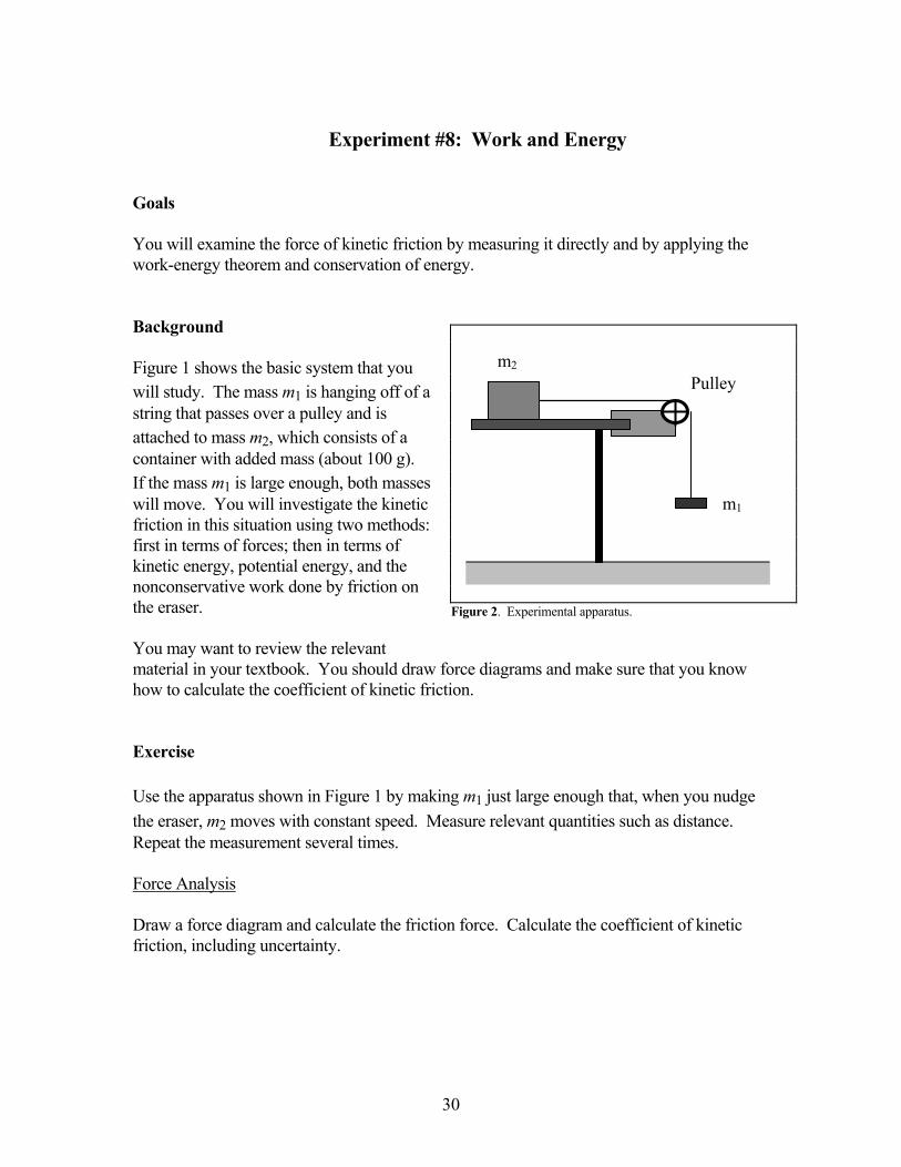
Experiment #8: Work and Energy Goals You will examine the force of kinetic friction by measuring it directly and by applying the work-energy theorem and conservation of energy. Background Figure 1 shows the basic system that you will study. The mass m1 is hanging off of a string that passes over a pulley and is attached to mass m2, which consists of a container with added mass (about 100 g). If the mass m1 is large enough, both masses will move. You will investigate the kinetic friction in this situation using two methods: first in terms of forces; then in terms of kinetic energy, potential energy, and the nonconservative work done by friction on the eraser. You may want to review the relevant material in your textbook. You should draw force diagrams and make sure that you know how to calculate the coefficient of kinetic friction. Exercise Use the apparatus shown in Figure 1 by making m1 just large enough that, when you nudge the eraser, m2 moves with constant speed. Measure relevant quantities such as distance. Repeat the measurement several times. Force Analysis Draw a force diagram and calculate the friction force. Calculate the coefficient of kinetic friction, including uncertainty.

Figure 2. Experimental apparatus.

Pulley m2

m1

31

Energy Analysis Calculate the change in mechanical energy. Use the work-energy theorem to calculate the friction force. Calculate the coefficient of kinetic friction, including uncertainty. Compare the values for the friction coefficient found in the two parts of this experiment: Are they consistent within your calculated deviations? Report You will turn in your analysis, discussion, and conclusions.

32

Experiment #9: Work and Thermal Energy Goals You will examine conservation of energy and the transformation of energy from one form to another. You will also determine the specific heat of lead. Background If an object does not change phase, then the change in its thermal energy (or internal energy), ∆E, depends directly on the change in its temperature, ∆T:

where m is mass and c is specific heat. According to conservation of energy, therefore, if an object falls a total height of h and all of its mechanical energy is converted to thermal energy of the object, then

You will use Equation 2 to determine the specific heat of lead. Note that equation 2 assumes that thermal energy is not lost to the environment. Exercise Caution: If ingested, lead is bad for you, but it is not absorbed through the skin. Avoid

spilling the shot. If you handle the lead, wash your hands afterwards. Please don't eat the apparatus.

Tape over the inside holes in the rubber stoppers. You will do a total of three trials; for each trial, use about one-third of the lead. Measure the mass and initial temperature of the shot. Pour the shot into the tube and close the tube up with the stoppers. Turn the tube over so that the shot falls the length of the tube without sliding down the side of the tube; turn the tube quickly, make sure that it is vertical, and ensure that all of the shot has reached the bottom before you turn the tube again. Repeat until the shot has fallen at least 200 times. Using a paper funnel, carefully and quickly pour the shot back into a cup and measure its final temperature. Measure the length of the tube. Repeat the experiment for a total of three trials. Record all pertinent data. Compute the specific heat for each trial. Combine the trials and compute the average and average deviation of the specific heat. Compare your results with the accepted value.

∆ ∆E = mc T , (1)

mgh = mc T .∆ (2)

33

In your discussion, explain why the heat loss to the surroundings produces a systematic error that makes your measured final temperatures smaller than they would be without the heat loss. Also explain why that would make your calculated specific heat systematically too large. Identify other sources of systematic error in the experiment, and state whether each source would make your calculated specific heat too small or too large. Suggest a procedure to measure, minimize, or eliminate each source of systematic error. Question To minimize the systematic error produced by heat loss, you could start with lead shot cooled below room temperature by 5°C, then drop the shot in the tube until its temperature is 5°C above room temperature. Explain why this procedure would help reduce the error. Report You will turn in a summary of your results, a discussion, and a conclusion. Also answer the question given above.

34

Experiment #10: Thermal Energy and Phase Changes Goals You will continue to examine the conservation of energy and the transformation of energy from one form into another. You will also determine the latent heat of fusion of ice. Finally, you will learn how you can minimize systematic error through your experimental procedure. Background Adding thermal energy to a system can increase its temperature or change its phase. For instance, when you add thermal energy to ice, it warms up to 0°C, changes to water at 0°C, then continues increasing temperature. As the ice melts, thermal energy from the surroundings converts to potential energy of the water molecules as the bonds between molecules weaken. In this experiment, you will melt ice in warm water and apply conservation of energy to determine the latent heat of fusion of ice. You should review the relevant sections of your text. The system will consist of water, ice, and an aluminum cup and stirrer. The main source of systematic error in this experiment is the thermal energy exchange between the system and the room. To compensate for this, you will start with water that is warmer than room temperature and end with water that is cooler than room temperature. Then, the thermal energy flowing out of the system when the water is warmer than room temperature will tend to cancel out the thermal energy flowing into the system when the water is cooler than room temperature. Exercise Measure room temperature. Weigh the dry calorimeter inner cup and stirrer. Add about 200 g of warm water (temperature about 5°C above room temperature) and weigh again. Assemble the calorimeter and insert the thermometer. Stir the water gently. Obtain about 30 g to 40 g of ice and dry it off. Place the ice in the calorimeter. Continue stirring and taking temperature readings until the temperature reaches its lowest point. Remove the calorimeter cup and weigh it again. Repeat the experiment. Apply conservation of energy to the system consisting of the calorimeter cup and stirrer, the original water, and the ice, treating the heat of fusion of ice as unknown. The energy equation will include the ice, the original water, the melted ice, and the calorimeter. Solve

35

for the heat of fusion of ice in terms of the temperature changes that you have measured; assume that the ice starts at 0°C. The specific heat of water is 4186 J/(kg×°C) and that of aluminum is 900 J/(kg×°C). Calculate the heat of fusion for each trial. Calculate the average and average deviation of your values for the heat of fusion of ice. Discuss the consistency of your result with the accepted value. Include all other required material in your report. Questions 1. Why was it necessary to wipe the ice dry before putting it into the calorimeter cup? How

would your results be affected if you did not? 2. From your temperature readings before you added the ice and your readings after the

water reached its lowest temperature, did the thermal energy exchange with the room indeed cancel out? Explain your answer. If the answer is "no", discuss the effects on your results; be as specific as possible.

Report You will turn in a full report. Include answers to the questions given above.

36

Experiment #11: Momentum, Collisions, and Mass Goals In this experiment, you will learn to use a photogate and a computer to measure the speed of a moving object. You will also study various types of collisions between rolling carts. You will apply conservation of momentum to determine mass ratios, and you will test the validity of conservation of mechanical energy. The experiment emphasizes developing and understanding the reasons for your procedure. Background Use of Photogates A photogate consists of a light emitter pointed at a light detector. When the space between the emitter and detector is empty, light hits the detector. When the space is blocked, light does not hit the detector. The electrical state of the detector depends on whether light hits it, allowing an electronic circuit to tell whether something is blocking the photogate. The photogate can be used to measure time intervals. Exercise To help you measure time accurately, you will use photogates connected to a computer through the Universal Lab Interface (ULI). See the document Lab Pro and Logger Pro. Run the timing program. Try blocking and unblocking the photogate and observing the program's output until you understand how to use a photogate to measure the length of time that the photogate is blocked. Then, use the one photogate to determine the speed of a single cart. Now, convince your instructor that you know how to acquire and interpret your data. Perfectly Inelastic Collisions Place the carts on the track so that, when they collide, the Velcro will make them stick together. Start with one cart ("target") stationary and the other cart ("projectile") moving. The target should have extra mass, but the projectile should not have extra mass. Only the projectile should have a card on it.

Connect a second photogate to the lab interface. Set up the photogates so that one measures the speed before the collision while the other measures the speed after the

37

collision. Try to position the photogates so that friction will have minimal effect on your results. Test conservation of momentum. Test conservation of mechanical energy. Elastic Collisions Orient the carts so that that the magnets in them make them bounce without actually hitting. Start with neither cart having extra mass and one cart stationary. Both carts must now have cards on them. Test conservation of momentum (remember that momentum is a vector). Test conservation of mechanical energy. Report You will turn in your data (including your procedure) and your analysis.

38

Experiment #12: Design of an Experiment Goals You will design and carry out an experiment. Exercise Choose a topic relating to this course. The topic should be specific enough for a short experiment. Form a hypothesis or pick some quantity to measure. Design, perform, and analyze an experiment to test that hypothesis or measure that quantity. Your experiment should be controlled and reproducible. Discuss sources of error in your experiment, and comment on how you could improve your experiment. Possible Topics Friction (focus on some particular aspect) Conservation of angular momentum (apparatus available) Bounciness of balls Conservation of momentum in collisions Height of a cloud Pressure and fluid velocity (for example, a squirt gun) Heat conduction Thermal radiation and temperature change Speed of sound Oscillation of a spring Report You will turn in a full report for this experiment.