, , ,Phone: 301-8236212, Fax: 301-8238249, 8226204

Abstract

The ready availability of credit on easy terms has proved to be instrumental in stimulating

agricultural investments until the 1970's. After that period, there was a marked slow-down ininvestment activity, a trend that characterised the entire Greek economy. This is primarily due tothe fact that since then credit had been increasingly tight.

The aim of this paper is, on the one hand, to quantify Greek farmers' investment behaviourboth at the aggregate level and by broad type of investment and, on the other hand, their demandfor loans to finance this investment. Thus, a simultaneous equations econometric model was usedto describe the demand for credit and investment by Greek farmers. In particular, credit needs foragricultural investment were estimated using a combination of a partial adjustment model and theadaptive expectations model. Farmers' investment behaviour was examined by employing asynthesized traditional model for aggregate and three types of investment. The rationalexpectations model is alternatively used. The traditional model was estimated by the 2SLS methodand the rational expectations model by the generalized method of moments. Then, the empiricalresults derived from the rational expectations model are compared with those obtained from theapplication of the traditional model. Finally, the main findings are summarized and some policyimplications are drawn.

An earlier version of this paper was presented at the International Conference on : "EconomicIntegration and Public Policy: NAFTA, The EC and Beyond" Toronto, Canada, May 26-28,1996

1.Introduction.*

The aim of this paper is to quantify, on the one hand, Greek farmer's investment behaviour

both at the aggregate level and by broad type of investment, and on the other hand, their demand

for loans to finance this investment. Such a quantitative approach to these two closely interrelated

issues should provide valuable guidelines in any attempt to formulate efficient credit policies for

institutional lenders to the farming sector.

A simultaneous equations econometric model was used to describe the demand for credit

and investment by Greek farmers. In particular, credit needs for agricultural investment were

estimated using a combination of a partial adjustment model and the adaptive expectations model.

Farmers' investment behaviour was investigated by employing a synthesized traditional model for

both aggregate and three individual types of investment.

Since the classical econometric model of adaptive expectations and partial adjustment

have been criticised, mainly for their inadequate theoretical basis, the rational expectations model

is alternatively used. Then, the empirical results derived from the rational expectations model are

compared with those obtained from the application of the classical model.

The paper has seven sections. In the second section, the developments with regard to

* I am indedebted to A. Andrikopoulos and P. Grevenites for their comments. Many thanks arealso due to E. Vasilatos for computational assistance.

application of the classical model. Finally, the main findings are summarized and some policy

implications are drawn.

2. Credit and capital formation policy in Greek agriculture

Between 1950 and 1992, total gross fixed asset formation in Greek agriculture increased in

real terms at an average annual rate of 2.6%. The year-on-year rates of increase were

considerably higher during the period up to 1973. After that year, there was a marked slow-down

in investment activity, which accelerated again in the eighties, with the exception of 1977 and

1985. This phenomenon has also characterised the entire Greek economy (Baltas and Sakellis,

1988). Here, too, we observe more-or-less the same trend in private investment, despite the

financial support provided to the agricultural sector by FEOGA since 1981.

In the same period, the shares of agricultural gross value added in GDP and of agricultural

investment in total investment gradually declined, with minor yearly fluctuations, from 33% and

10% in 1950 to 15% and 6% in 1990 respectively, reflecting the farming sector's decreasing

weight in the overall economy as the industrialisation process got under way. When we break total

agricultural investment into its private and public components, we observe a fairly steady

relationship on 1:2 in favour of private investment, except for a few years in the early sixties and in

the late eighties (Diagram 1), when the private and public components of agricultural investment

were almost equal.

Private fixed asset formation in agriculture is broken down in official statistical sources into

the following types of investment: (i) non-residential buildings, (ii) machinery and equipment and

(iii) other constructions and works. The bulk of private investment -around half or more-went to

1973 and then, showing a declining trend, more-or-less stabilized at considerably lower levels. As

for public agricultural investment, by far the largest share, around nine tenths or more, was

channelled to fixed assets other than machinery and equipment and, predominantly, to land

improvements, which alone typically took up to three fifths or more of the total.

Turning now to the financing of private investment activity in the farming sector, the first

thing to note is that until very recently the exclusive institutional lender to agriculture had been the

state-owned Agricultural Bank of Greece (ABG). As a result, bank financing of the primary sector's

investment is no other than the amount of medium and long-term credit extended by the ABG.

Throughout the post-war period and up to the early eighties, an easy credit policy was adopted

towards the farming sector. The main tools were a low interest rates regime (many of which were

subsidised), longer pay-off periods, etc. The rationale for this treatment is twofold: first, the

recognition, given the overwhelmingly family character of Greek agriculture, of owner-occupiers'

limited scope for self-finance; second, the provision of a strong incentive for the sector's

modernization and structural improvement.

Since 1984, credit has been increasingly tight, because of the liberalization of the banking

system following Greece's entry to the E.C. (Diagram 3). Controls imposed on the size of

agricultural credit and its allocation among various crops started to relax and were eventually

removed. The final stage in this development was the conversion of the ABG from a state-owned,

specialized institutional lender to a "normal" bank with the legal status of societe anonyme, whose

sole shareholder, however, is the Greek State.

Throughout the period under discussion, ABG loans covered about 50% of private farm

investment. In fact, ABG finance has followed the same trend as that of private farm investment.

Thus, ABG loans as a percentage of private farm investment increased from 39% in 1958 to 71%

agriculture showed relative stability in relation to the rapid and frequent fluctuations of the inflation

rate (Diagram 5). In fact, the adjustment of interest rates to changes of inflation occurred at

considerably lower levels and with a time lag, except in the 1957-63 and 1987-92 subperiods. The

recent developments in interest rates and their adjustment to levels equal to or even higher than

inflation rates are a major factor in the drop in the demand for loanable funds by farmers (Diagram

5).

Regarding the share of ABG loans by type of investment, we notice that in the case of

"non-residential buildings"1 these ranged from 70 to 90 percent, while for "machinery and other

equipment" ABG's share fluctuated between 14 and 86 percent. Lastly, bank lending for "other

constructions and works" covered 40 percent of realised investment of this type, the major part of

which was granted at subsidised interest rates until the late 1970's (Baltas, 1980).

3. The econometric model

In order to describe the interrelationship between financing and capital formation at the

aggregate level and by type of investment, a simultaneous equations econometric model was

employed comprising two behavioural equations: investment finance and private investment

expenditure.

1 For a few years the share of ABG loans in investment on "non-residential buildings" exceeded100 percent. This can be attributed to the fact that some investment projects might have beenrealized first and financed by the ABG later when the required credits had become available.

of investment *t( )I 2 and of the nominal interest rate t( )r 3 :

* *t t t0 1 2 t = + + + a a a uM I r 4 (1)

It is further assumed that the farmer gradually adjusts the actual level of financing to the desired

level, depending on progress made in carrying out the investment projects and the availability of

finance by the ABG. The rate of adjustment of actual financing towards a new equilibrium position

depends on the difference between the current desired level of financing and the past actual level,

as well as on the speed of adjustment of the desired level to the actual one:*

t t-1 t t-1 t - = ( - ) + 0 < vM M M Mλ λ 5 (2)

Equation (2) indicates the way by which the actual level of financing adjusts towards its long-run

equilibrium. The coefficient of adjustment (λ) represents the proportion of the adjustment towards

equilibrium which occurs in a given time period. The adaption of investment towards the desirable

level takes place according to the adaptive expectations model which postulates that the expected

investment is adjusted in each time period by a proportion of the difference between the current

period's actual investment t( )I 6 and its previous period expected

investment.

* * *t t-1 t t-1 t - = ( - ) + 0 < 1wI I I Iµ µ ≤ 7 (3)

Equation (3) can be written:*t t t(1 - L + L) = + wI Iµ µ 8, (4)

where L is the lag operator. Therefore equation (2) becomes*t t t = (1 - L + L) + vM Mλ λ 9 (5)

Substituting equation (4) and (5) into (1) and re-arranging terms we obtain:

t t t-1 t-2 t t-10 1 2 3 4 5 t = + + + + + + b b b b b bM I M M r r ε 10, (6)

will be immediate and full (Alogoskoufis and Baltas, 1991, p.83). The reduced form simplifies to

t t t-1 t0 1 2 3 t = + + + + b b b bM I M r′ ′ ′ ′ ′ε 12, (7)

where0 0 1 1 2 3 2

4 3 t t t t

= , = , = 1- , = , b a b a b b a = , = ( + ) + . b a u w v

′ ′ ′

′ ′

λ λ λ λλ λε

13

Assuming that equations (1), (4) and (5) have been expressed in log-linear form3, we can

obtain the investment finance equation in a double-log formulation.

t t t-1 t-2 t0 1 2 3 4 tlog = + log + log + log + log + c c c c c eM I M M r 14 (8)

In the case where µ=1, the double-log formulation is converted into:

t t t-1 to 1 2 3 tlog = + log + log + log + c c c c eM I M r′ ′ ′ ′ ′ 15. (9)

3.2Private investment expenditure

The traditional approach to modelling investment behaviour requires assumptions about

both the adjustment process and the desired level of capital. Various theories about the

adjustment process have been proposed. First, Koyck suggested a geometric distributed lag

2 Coefficients λ and µ enter asymmetrically in equation (6) and hence it is impossible toestimate them separately.

3 In the double-log form it is assumed: first, that the desired level of financing is a log-linearfunction of the desired level of investment; second, that the adjustment of financing is proportionalto the percentage difference between actual investment in the previous year and desiredinvestment in the current year; and, third, that the rate of growth of desired investment is anexponential function of the ratio of actual investment in the current period to desired investment inthe previous period. These assumptions refer to the expected values of logarithms.

The specification of desired capital has been based on four major theories. Clark's

approach (1917), known as capacity utilization, assumed that desired capital is proportional to

output because a firm's incentive to invest will increase with the output produced by capital. In

agriculture, Girao, Tomek and Maint (1974) found that the change in output between periods is

more appropriate to capture the demand for investment.

Third, Tinbergen (1938) proposed an alternative theory in which investment depends on

the level of expected future profits. Higher profitability increases future expectations - which in turn

stimulate current investment - and may also ease any constraints on the supply of funds to finance

expansion.

Part of the rationale for using expected profitability involves the importance of internal

liquidity. According to Campbell (1958), this "residual funds" hypothesis is relevant to agriculture

because the sector is comprised mostly of family-based production units. Capital formation is

achieved through the direct efforts of individual members and lower profitability or fewer available

internal funds may prevent attainment of the desired capital stock level much more readily than in

an industrial firm which has greater access to outside capital.

Jorgenson (1971), based on neoclassical theory, developed a model in which owners

maximize the present value of their equity under conditions of perfect competition. The optimal

capital stock is found by equating the marginal value product to its cost. Jorgenson and Siebert

(1968) were the first to incorporate the influence of tax structures in the cost of capital.

The traditional investment models have been criticised because they have been based on

ad hoc specifications for the adjustment process and desired capital level. More recent models

have cast the firm in a dynamic optimization framework in order to derive its investment behaviour

equation. Examples are found in Berndt, Buss and Waverman (1978) and subsequently in

behaviour with respect to aggregate and three distinct types of investment. The independent

theories were integrated into a single, unified approach, where desired capital *t( )K 17 is a

function of capacity utilization, tY∆ 18 (accelerator), the

expected revenues (profits), tY 19, the nominal interest rate,

tr 20, and public investment in the agricultural sector tG 21. Since

there is no unanimous agreement in applied economics on the

measurement of expected revenue and no data is available on the

latter, alternative variables are used: gross agricultural income

with a time lag of n years t-nY 22 or an implicit price deflator of

agricultural income with a time lag of n years, t-n.P 23

*t t t-n t-n t0 1 2 2 3 4 t = + + or + + d d d d d d GK Y Y P r′∆ 24. (10)

This equation for desired capital was substituted into Chenery's (1952) flexible accelerator model.*

t t t-1 t-1t = - = ( - )I K K KKλ 25 (11)

The resulting investment equation is

t t t-n t-n t t-10 1 2 2 3 4 t = + + or + + - .d d d d d d GI Y Y P r K′λ λ ∆ λ λ λ λ λ 26 (12)

Following Gardner and Sheldon (1975) and Waugh (1977a,b), the speed of adjustment is

then modeled as a linear function of available internal and external funds4 relative to desired

investment,t t2 3

1 *t t-1

+ Y = + - K K

λ λ Μλ λ 27, (13)

where 1 2 , λ λ 28 and 3λ 29 are constants to be determined. Completing

4 It is important to mention that, in the Greek case, bank financing covered 40 to 60% of privatefarm investment throughout the period.

ho=λ1 do; h1=λ1 d1; h2=λ1 d2+λ2; h3=λ1d2'+λ2; h4=λ1 d3; h5=λ1; h6=λ1d5; h7=λ3.

In a log-linear form, the investment model is

o 1 t 2 3 t-nt t-n = + log + or log logI logYh h Y h h P′ ′ ′∆′ 33

4 5 6 -1 7 ttt+ + log + log + log logr Gh h h h M′ ′ ′ ′τΚ 34. (15)

Parameters d2 and λ2 cannot be determined because the number of unknown is greater than the

number of equations.

4.The rational expectations model

The adaptive expectations and partial adjustment models have been criticised mainly for

their inadequate theoretical basis and the statistical estimation problems arising when the ordinary

least squares method is used5. The dynamic element in these models is introduced without a

formal theory but on the simple ad hoc assumption that in each period, if we are dealing without

discrete time, a fraction of the difference between the current period and the long-run equilibrium

is eliminated. The criticism also refers to the underpininning adjustment and expectations

mechanism in which these are expressed in terms of a geometric lag of past observations.

However, it is claimed that to impose this structure on the data is unacceptable from the point of

view of both economic theory and time series analysis because it is assumed that the expected

values of past observations follow a moving average procedure in their first differences, i.e ARIMA

5 See Baltas (1987), p.196.

yields, we can make use of a simplified model of rational expectations which consists of two

behavioural equations. We assume that farmers are rational in the sense, that they respond to the

various signals given out by the economic environment and formulate their own expectations

about their agricultural income taking into consideration developments in the CAP, credit policy,

etc.

The investment finance equation is given by*

t t t-1 t-2 t t-1o 1 2 3 4 5 t

1 2 3 5

= + + + + + + b b b b b b uM I M M r r> 0; > 0; < 0; > 0,b b b b

35 (16)

and the private investment expenditure equation is given by*

t o 1 t 2 t-n 3 t-n 4 t 5 6 t-1 7 tt t

1 2 3 4 5 6 7

= + + or + + + + + G vI h h Y h Y h P h r h h K h M> 0; > 0; > 0; > 0; > 0; < 0; > 0h h h h h h h

∆36(17)

where * *t t t-1 t t t-1 = E( / ) and = ( / )I I T M M T 37 are the farmers' current

expectations about investment expenditure and investment finance

respectively (E is the mathematical expectation and T denotes the

information set upon which expectations depend) and ut, vt are random

disturbances with zero means and a diagonal variance-covariance matrix.2

t u 12

2t 21 v

0 u _ N , 0 v

σ σ

σ σ 38 (18)

Solving equations (16) and (17) for the two endogenous variables Mt and It (having first

imposed the rational expectations hypothesis for It* = E(It/Tt-1) and Mt* = E(Mt/Tt-1)), we obtain the

following reduced form equations:

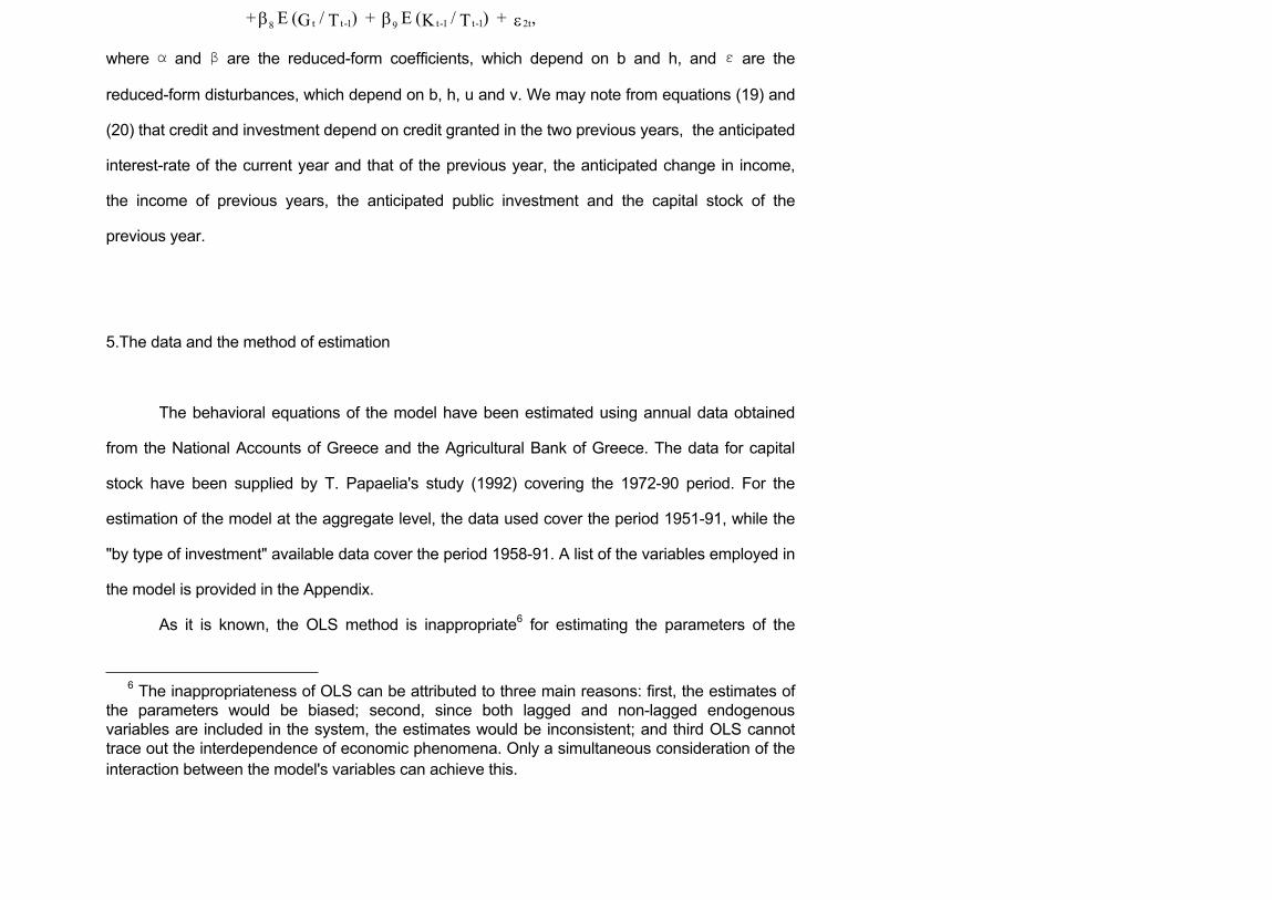
t-1 t-1 tt8 9 + E ( / ) + E ( / G T Kβ β -1 2t) + ,T ε

where α and β are the reduced-form coefficients, which depend on b and h, and ε are the

reduced-form disturbances, which depend on b, h, u and v. We may note from equations (19) and

(20) that credit and investment depend on credit granted in the two previous years, the anticipated

interest-rate of the current year and that of the previous year, the anticipated change in income,

the income of previous years, the anticipated public investment and the capital stock of the

previous year.

5.The data and the method of estimation

The behavioral equations of the model have been estimated using annual data obtained

from the National Accounts of Greece and the Agricultural Bank of Greece. The data for capital

stock have been supplied by T. Papaelia's study (1992) covering the 1972-90 period. For the

estimation of the model at the aggregate level, the data used cover the period 1951-91, while the

"by type of investment" available data cover the period 1958-91. A list of the variables employed in

the model is provided in the Appendix.

As it is known, the OLS method is inappropriate6 for estimating the parameters of the

6 The inappropriateness of OLS can be attributed to three main reasons: first, the estimates ofthe parameters would be biased; second, since both lagged and non-lagged endogenousvariables are included in the system, the estimates would be inconsistent; and third OLS cannottrace out the interdependence of economic phenomena. Only a simultaneous consideration of theinteraction between the model's variables can achieve this.

6. Empirical results

The use of the rational expectations model in our attempt to explain the interrelationship

between financing and capital formation in Greek agriculture does not always provide clearly

superior results to those obtained by the classical econometric model of adaptive expectations and

partial adjustment (see Tables 1 and 2). This will be made evident below when we consider

investment financing and capital formation at the aggregate level and by type of investment in

which the limited explanatory capacity is a feature of all rational expectations models employed in

our analysis.

In the case of the credit function for aggregate private investments (Table 1) we can see

that capital formation is the major explanatory variable while credit extended in the previous year

and the rate of interest only slightly affect the level of credit in the current period. As to the

insignificant influence exerted on the level of borrowing by the amount of credit supplied in the

previous year, this should be attributed to the fact that agricultural investment, and especially on-

farm investment, tends to be smaller scale and to have a shorter gestation period than that

undertaken in the other economic sectors. Similar results we reobtained in our previous study

(Baltas, 1983). Second, it should be noticed that the interest rate elasticity value is very low (-

0.07). This can be attributed to the credit rationing that prevailed over most of the period, which

made credit supply given for many farmers.

Turning now to the aggregate investment function, the decisive variable was medium - and

long - term credit (cf. Baltas, 1983). This is true for both econometric models. Farmers' decisions

buildings" we can notice that the two models are almost identical (Tables 1 and 2). Thus, the

speed of adjustment is the same for both credit and investment (µ=λ=0.9), which means that,

given its small scale, this type of investment is more or less completed within a single-year. With

regard to the investment equation, the empirical results reveal that credit is the decisive factor in

this case as well, whilst farmers' decisions to invest are influenced by the interest rate.

Next, we have the two functions relating to investments in "machinery and other

equipment". The results under the rational expectations model were not substantially different from

those under the classical econometric model. From the first equation, it is clear that the demand

for loans is related to the level of investment and to the interest rate. The partial adjustment

coefficient is λ= 0.99 and that of the adaptive expectations one is µ=1 . In other words, credit

adjustment takes place within a little over one year while the rate of investment adjustment is even

faster. This is explained by the ready availability of credit that has provided a strong incentive for

the mechanization of Greek agriculture for many years.

Coming now to investment in "machinery and other equipment", we notice that this is

heavily influenced by the level of agricultural income in the previous year implying a high elasticity

value (3). As for the capital stock, it does have the anticipated sign and seems to play a negative

role on farmers' decision to mechanize their production given the high degree of mechanization of

the farming sector in recent years and the sector's structural weakness (small and multi-

fragmented farms). In contrast to our previous study, the amount of credit fails the statistical

significance test in the classical model, although it passes the test in the rational expectations

model.

Finally, in the case of investment in "other constructions and works" a comparison of the

estimates arrived at under the two approaches reveals that the rational expectations model of the

Indeed, in the classical econometric model the level of investment in "other constructions and

works" is satisfactorily explained by the relevant amount of credit provided, by the level of farm

income in the two previous years and by the interest rate. The statistical significance of public

investment is explained by the fact that this variable is being overwhelmingly devoted to major

land improvement and irrigation schemes and its infrastructural character is a precondition for

undertaking on-farm investment.

In the classical econometric model of the credit equation, it is worth noting the strong

influence exerted by the medium -and long-term loan variable lagged by two years, in contrast to

what we found in the previous two types of investment. The obvious reason for this divergence is

that because this category of investment mainly refers to on-farm land improvement and irrigation

projects and to tree and vineyard planting, a longer gestation period is necessary.

7. Concluding remarks and policy implications

Having compared the empirical results obtained by the classical econometric model with

those obtained by the rational expectations model, it is evident, on the basis of economic criteria,

that one cannot be in favour of the latter approach. On the contrary, in two cases results were less

satisfactory (aggregate private investment and other constructions and works). In the case of

machinery and other equipment a slight improvement was observed while remained the same in

non-residential buildings.

Overall, the empirical analysis shows that capital formation is the major explanatory

variable of the demand for credit followed in some cases by the credit extended in the previous

1980's.

o 1 2 = -5.833, = 1.633, = - 0.059, = = 1a a a λ µ

t t-2 t t

t

2

(b) = - 2.569 + 0.682 - 0.183 0.270 logRI logRY logr logG

(1.356) (3.034) (2.117) (2.714)

+ 0.232 logRM

(2.262)

N = 37, = 0.930, DW = 2.0R 1 2ˆ ˆ64, = 0.479, = - 0.400 R R (2.825) (2.333)

42

Rational Expectations Model

t t t-1 t

2

o

(a) log = -5.373 + 1.548log + 0.034log - 0.069logrRM RI RM (5.698)(11.039) (0.479) (1.118)

N = 35, = 0.846, DW = 1.497 R

= - 5.562, a 1 2 = 1.602, = - 0.071, = 1, = 0.966a a µ λ

43

t t-2 tt

2

(b) log = -3.048 + 0.672log - 0.153 + 0.592loglogrRI RY RM (3.335) (5.201) (2.401) (7.878)

N = 35, = 0.841, DW = 1.472 R

44

7 Figures in parentheses denote t-statistics. The values 1R̂ Error! Main Document

Only. and 2R̂ Error! Main Document Only. express the first- andsecond- order autoregressive coefficients. The values a0, a1, a2, µ and λshow the estimates of the parameters of equations (1), (2) and (3).

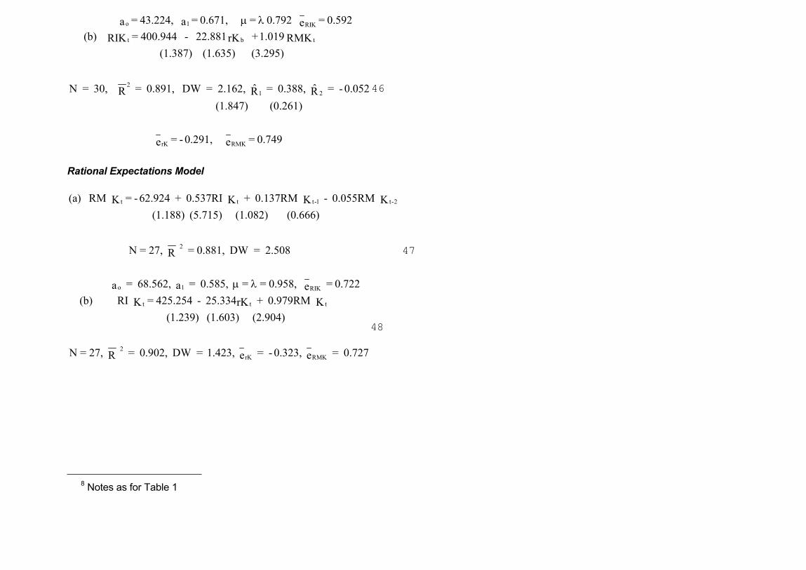
o 1 RIK

= 43.224, = 0.671, = 0.792 = 0.592a a eµ λ

t b t

21 2

(b) = 400.944 - 22.881 + 1.019 RIK rK RMK (1.387) (1.635) (3.295)

ˆ ˆN = 30, = 0.891, DW = 2.162, = 0.388, = - 0.052R R R

rK RMK

(1.847) (0.261)

= - 0.291, = 0.749e e

46

Rational Expectations Model

t t t-1 t-2

2

o 1

(a) RM = - 62.924 + 0.537RI + 0.137RM - 0.055RM K K K K (1.188) (5.715) (1.082) (0.666)

N = 27, = 0.881, DW = 2.508 R

= 68.562, = 0.58a a RIK5, = = 0.958, = 0.722eµ λ

47

t t t

2rK RMK

(b) RI = 425.254 - 25.334 + 0.979RM K rK K (1.239) (1.603) (2.904)

N = 27, = 0.902, DW = 1.423, = - 0.323, = 0.727e eR

48

8 Notes as for Table 1

o 1 2

RIM rM

= 683.826, = 0.313, = - 42.625, = 1 = 0.965 a a a

= 0.808, = - 0.610e e

µ λ

t t-1 t-1 t

21

(b) = - 2985.915 + 60.798 - 0.118 + 0.498 RIM RPY MK RMM (1.078) (2.270) (1.467) (0.860)

ˆ N = 17, = 0.424, DW = 2.165, = 0.004,R R

-1 -1 RMMRPY MK

(0.019)

= -3.267, = -1.158, = 0.186e e e

50

Rational Expectations Model

t t t-1 t

2

o 1 2

(a) RM = -361.772 + 0.412RI + 0.009RM - 36.529M M M rM (0.960) (3.251) (0.047) (2.588)

N = 17, = 0.675, DW = 1.589 R

= 365.057, = 0.416, a a

RIM rM

= -36.861, = 1, = 0.991, a

= 1.127, = - 0.547e e

µ λ51

9 Notes as for Table 1

tt t-2 t

t

(b) = - 0.786 + 0.516 - 0.047 + 0.225 logRIL logRY logGrL (0.444)(2.905) (4.624) (1.964)

+ 0.153 logRML

(2.208)

21 2

ˆ ˆN = 30, = 0.863, DW = 2.473, = 0.021, = - 0.688 R R R (0.136) (4.401)

54

Rational Expectations Model

t t t-2

2

(a) log RM = -3.538 + 1.181log RI + 0.239log RM L L L (2.153)(3.786) (1.421)

N = 27, = 0.665, DW = 1.959 R

55

t t tt-2 t

2

(b) log RI = -5.392 + 0.936 - 0.069 + 0.468 + 0.099logRM logRY logGL rL L (2.153)(1.376) (2.431) (1.932) (0.456)

N = 27, = 0.764, DW = 1.867 R

56

10 Notes as for Table 1

Endogenous variablesRM:Medium-and long-term loans for agricultural private investment deflated by the implicit price

index of agricultural private investment, P,(1970=100).RI:Agricultural private investment at constant 1970 prices.RMK:Medium-and long-term loans for agricultural private investment in non-residential buildings

deflated by the implicit price index of agricultural private investment in non-residential buildings, PK, (1970=100).

RIK:Agricultural private investment in non-residential buildings at constant 1970 prices.RMM:Medium-and long-term loans for agricultural private investment in machinery and other

equipment deflated by the implicit price index of agricultural private investment inmachinery and other equipment, PM, (1970 = 100).

RIM:Agricultural private investment in machinery and other equipment at constant 1970 prices.RML:Medium-and long-term loans for agricultural private investment in other constructions and

work deflated by the implicit price index of agricultural private investment in otherconstructions and works, PC, (1970 = 100).

RIL:Agricultural private investment in other constructions and works at constant 1970 prices.

Predetermined variablesRM-i:Real medium- and long-term loans for agricultural private investment lagged i years (i=1,2).RMK-i:Real medium - and long-term loans for agricultural private investment in non-residential

buildings lagged i years (i=1,2).RMM-i:Real medium- and long-term loans for agricultural private investment in machinery and

other equipment lagged i years (i = 1,2).RML-i:Real medium- and long-term loans for agricultural private investment in other constructions

and works lagged i years (i = 1,2).∆Y:Changes in gross agricultural income at constant 1970 prices.RY-n:Gross agricultural income lagged n years at constant 1970 prices.RPY-n:Implicit price index of agricultural income deflated by the implicit price index of gross

domestic product (1970=100).r:Nominal interest rate paid for medium - and long-term loans for agricultural private investment.

KK-1:Agricultural private capital stock in non-residential buildings lagged one year at constant 1970prices.

MK-1:Agricultural private capital stock in machinery and other equipment lagged one year atconstant 1970 prices.

LK-1:Agricultural private capital stock in other constructions and works lagged one year at constant1970 prices.

Baltas, N. (1987), Supply Response for Greek Cereals , European Review of AgriculturalEconomics, 14:195-220.

Baltas, N. (1983), "Modelling Credit and Private Investment in Greek Agriculture", EuropeanReview of Agricultural Economics, 10:389-402.

Baltas, N. (1980), "An Empirical Investigation of the Production and Trade of Greek Peaches",Oxford Agrarian Studies, 9:89-114.

Berndt, E., M. Fuss and L. Waverman (1978), Dynamic Models of the Industrial Demand forEnergy, Electric Power Research Institute, Palo Alto CA.

Box, G.E.P. and Jenkins, G.M. (1970).Time Series Analysis, Forecasting and Control, Holden-Day, San Francisco.

Cambell, K.O. (1958) "Some Reflections on Agricultural Investment", Australian Journal ofAgricultural Economics, 2: 93-103.

Cherery, H.B. (1952) "Overcapacity and the Acceleration Principle", Econometrica, 20:1-28.Clark, J.M. (1917), "Business Accelerations and the Law of Demand: A Technical Factor in

Economic Cycles", Journal of Political Economy, 25:217-35.Gardner, R., and R. Sheldon (1975), "Financial Conditions and the Time Path of Equipment

Expenditures", Revue of Economics and Statistics, 57:164-70.Girao, J.A., W.G. Tomek, and T.D. Mount (1974), "The Effect of Income Instability on Farmers'

Consumption and Investment", Revue of Economics and Statistics, 56:141-50.Hansen, L.P. and K.J. Singleton (1982), "Generalized Instrumental Variables Estimators of

Nonlinear Rational Expectations Models", Econometrica, 50:1269-86.Jorgenson, D.W. (1971), "Economic Studies of Investment Behavior: A Survey", Journal of

Economics Literature, 49:1111-47.Jorgenson, D.W. and C.D. Siebert (1968), "A Comparison of Alternative Theories of Corporate

Investment Behavior", American Economic Revue, 58:681-712.LeBlank, M. and J. Hrubovcak (1985), "The Effects of Interest Rates on Agricultural Machinery

Investment", Agricultural Economic Research, 37:12-22.LeBlank, M. and J. Hrubovcak (1986), "The Effects of Tax Policy on Aggregate Agricultural

Investment", American Journal of Agricultural Economics, 68:767-77.Narayana, N.S.S. and Shah, M.M. (1984), "Farm Supply Response in Kenya: Acreage Allocation

Econometrica, 48(1):49-73.Waugh, D.J.(1977), "The Determinants and Time Pattern of Investment Expenditures in the

Australian Sheep Industry", Quarterly Revue of Agricultural Economics, 30:150-161.Waugh, D.J. (1977), "The Determinants of Investment in Australian Agriculture - A Survey of

Issues" Quarterly Revue of Agricultural Economics, 30:133-49.Weersink, A.J. and Tauer, L.W. (1989), "Comparative Analysis of Investment Models for New York

Dairy Farms", American Journal of Agricultural Economics, 71:136-145.