phase-shifting interferometry based on induced vibrationseprints.ucm.es/22321/1/quirogaja15.pdf ·...

Phase-shifting interferometry based on induced vibrations

J. Vargas,1,*

J. Antonio. Quiroga,2 A. Álvarez-Herrero

1,

and T. Belenguer1

1 Laboratorio de Instrumentación Espacial, Instituto Nacional de Técnica Aeroespacial, Carretera de Ajalvir Km. 4, 28850, Torrejón de Ardoz (Madrid), Spain

2 Optics Department, Universidad Complutense de Madrid, Facultad de CC. Físicas, Ciudad Universitaria s/n, 28040 Madrid, Spain

*[email protected]

Abstract: The presence of uncontrolled mechanical vibrations is typically the main precision-limiting factor of a phase-shifting interferometer. We present a method that instead of trying to insolate vibrations; it takes advantage of their presence to produce the different phase-steps. The method is based on spatial and time domain processing techniques to compute first the different unknown phase-steps and then reconstruct the phase from these tilt-shifted interferograms. In order to compensate the camera movement, it is needed to perform an affine registration process between the different interferograms. Simulated and experimental results demonstrate the effectiveness of the proposed technique without the use of any phase-shifter device.

©2011 Optical Society of America

OCIS codes: (050.5080) Phase shift; (120.3180) Interferometry; (120.5050) Phase measurement.

References and links

1. K. Creath, ―Phase-shifting interferometry techniques,‖ Prog. Opt. 26, 350–393 (1988). 2. D. Malacara, M. Servín, and Z. Malacara, Interferogram analysis for optical testing, (Marcel Dekker, Inc, 1998) 3. K. A. Goldberg, and J. Bokor, ―Fourier-transform method of phase-shift determination,‖ Appl. Opt. 40(17),

2886–2894 (2001). 4. Z. Wang, and B. Han, ―Advanced iterative algorithm for phase extraction of randomly phase-shifted

interferograms,‖ Opt. Lett. 29(14), 1671–1673 (2004). 5. M. Chen, H. Guo, and C. Wei, ―Algorithm immune to tilt phase-shifting error for phase-shifting interferometers,‖

Appl. Opt. 39(22), 3894–3898 (2000). 6. A. Dobroiu, D. Apostol, V. Nascov, and V. Damian, ―Tilt-compensating algorithm for phase-shift

interferometry,‖ Appl. Opt. 41(13), 2435–2439 (2002). 7. J. Xu, Q. Xu, and L. Chai, ―Tilt-shift determination and compensation in phase-shifting interferometry,‖ J. Opt.

A, Pure Appl. Opt. 10(7), 075011 (2008). 8. Z. Ge, and M. Takeda, ―Self-reference method for phase-shift interferometry,‖ Proc. SPIE 4416, 152–157 (2001). 9. G. Rodriguez-Zurita, N. I. Toto-Arellano, C. Meneses-Fabian, and J. F. Vázquez-Castillo, ―One-shot phase-

shifting interferometry: five, seven, and nine interferograms,‖ Opt. Lett. 33(23), 2788–2790 (2008). 10. R. Hartley, and A. Zisserman, Multiple View Geometry in Computer Vision, (Cambridge University Press, 2004). 11. C. Harris, and M. J. Stephens, ―A combined corner and edge detector,‖ in Alvey Vision Conference, pp. 147–152

(1988). 12. J. C. Wyant, and K. Creath, ―Basic Wavefront Aberation Theory of Optical Metrology,‖ in Applied Optics and

Optical Engineering, Vol. XI, Chapter 1, Academic Press (1992).

1. Introduction

Among wave-front reconstruction techniques based on automated interferogram analysis methods, the Temporal Phase-shifting Interferometry technique (TPI) is accepted as the most precise and accurate one [1]. The theoretical high accuracy of this technique is limited by many sources of error [2] as all errors related with the phase-shift fidelity, including the phase-shifter performance and measurement environment instabilities. The precision and accuracy lost in TPI caused by vibrations limit the application range of these techniques to a very controlled and stable laboratory environment. If the presence of these mechanical

#128619 - $15.00 USD Received 18 May 2010; revised 2 Aug 2010; accepted 4 Aug 2010; published 5 Jan 2011(C) 2011 OSA 17 January 2011 / Vol. 19, No. 2 / OPTICS EXPRESS 584

environment instabilities is low, phase-shifting calibration procedures or self-calibration algorithms can be used to accurately reconstruct the unknown phase [3,4]. These methods assume that the phase-steps are constant for all pixels in one interferogram but typically different between interferograms. If the phase-shifter introduces non-uniform phase-shift steps along the aperture, this assumption is not longer valid and appears a tilt-shift error [5–8]. This situation usually appears when the phase-shifter —typically a PZT device— has orientation errors during the shift. A scheme of this situation is shown in Fig. 1 where a phase-shifter device it is shown in three different positions. If the phase-shifter has orientation errors during its movement the phase-shifting will be corrupted by a tilt-shift error that will be different for each interferogram.

Fig. 1. Scheme of a PZT Phase-Shifter device with tilt-shift error

Several methods have been proposed to eliminate the tilt-shift error. In Ref [5]. an algorithm immune to both translational and tilt-shift errors is presented. In this case, the principle of the algorithm is to use a first order Taylor series expansion of the phase-shifting errors instead of the original nonlinear phase-error equations; then by iteration the phase-shift plane is determined. In Ref [6], it is presented a phase-shifting demodulating method based on dividing the interferograms into small regions, where the phase-shifting can be considered approximately constant; a self-calibrating approach is applied in each block. In [7] a combined spatial and temporal demodulating method is presented. First, a spatial demodulation is performed by a FFT based method. Second, the previously calculated phases are subtracted with respect to the first one, in order to obtain the different tilt-shift errors with respect to the first phase. Finally, by a least-square iterative minimization process the true phase map and the different tilt errors are determined. In Ref [8]. a self-reference method is proposed for phase-shifting interferometry when translation and tilt errors exist. Another strategy to deal with this kind of problems can be using a one-shot phase-shifting interferometry method [9]. This approach allows recovering at the same time different interferograms at the camera detector. The main drawbacks of this method are that, on one hand it is necessary to share the camera detector between N interferograms and therefore the spatial resolution of the measured phase will be decreased. On the other hand, this method requires a matching procedure between the different interferograms that can be problematic in some cases

The mentioned methods [5–8] are not directly applicable in the case of a measuring system with severe mechanical vibrations. The method presented in Ref [5]. is based on a first order Taylor approximation of the tilt-shift errors so it is assumed that these tilt-shift errors are small compared with the problem phase. In [6] it is needed to establish beforehand the size of the processing block. If the phase-shifting error is large compared with the problem phase, the size of processing blocks must be very small and therefore the result of the iterative self-


calibration algorithm can be not trustful. In presence of severe vibrations, a new problematic that appears and that cannot be solved with any of the methods exposed above [3–8] is the phase-error introduced by the movement of the camera. Note that if these vibrations introduce a camera movement the corresponding interferogram pixels will not match. In this case, the camera oscillation introduces a set of unknown affine transformations between interferograms in temporal phase-shifting. In typical mechanical stabilized temporal phase-shifting interferometry these affine transformations can be neglected, but this is not the case if severe vibrations are presented. An example where it is interesting to obtain interferometric data but it is impossible using the typical temporal phase-shifting methods is inside a thermal-vacuum chamber. The use of interferometry inside these chambers is important because it permits to obtain optical quality measures of optical components at different ranges of temperature and pressure that for example, it is necessary in space applications.

In this paper, we present a method that instead of trying to insolate vibrations; it takes advantage of their presence to produce the different phase-shifts. The method is based on spatial and temporal demodulation and can be divided in three steps. First, a set of interferograms are acquired in different times. A spatial fringe demodulation process by a Fourier transform method is achieved over each interferogram. Second, using the initial estimation of the phase, the different tilt-shifts and affine transformations are obtained. Finally, using the previously computed affine transformations, the different interferograms are referred to a unique camera frame and then a general demodulation technique based on a least-squares iterative minimization process is performed using the previously computed tilt-shifts. Note that using a temporal sequence of N interferograms to obtain the modulating phase by a TPI technique is more accurate that obtaining the phase from a single interferogram by the Fourier transform method. On one hand, the TPI method reduces errors in phase calculations when noisy interferograms are involved [2]. Additionally, the Fourier method suffers from border effects that introduce additional errors in the recovered phase. Our method makes possible to obtain interferometric measurements in very hostile environments as thermal-vacuum chambers, where severe shock vibrations with a typical frequency of 0.5 Hz and induced displacements in the range of millimeters appear caused by the cryogenic pump. Additionally, the proposed method also permits to acquire interferometric measures without the need of any phase-shifter device.

2. Proposed method

The proposed method is divided in three steps. First, it is determined the tilt-shift in each interferogram. Second, it is obtained the affine transformations between interferograms and finally, the phase is computed by a general temporal demodulation method based on the least-squares method.

2.1 Tilt-shift determination by the Fourier transform method

For the sake of clarify; we first assume that we have a mechanically stabilized interferometer in which the phase-shifts are introduced by a PZT device. In this case, the intensity at camera

pixel ,x y of the nth

interferogram can be represented as,

0, , , cos ,n nI x y A x y B x y x y d (1)

where, nI is the theoretical intensity of the nth interferogram, ,A x y is the background

intensity, ,B x y is the modulation of fringe pattern, nd is the phase-shift introduced by the

PZT device and 0 ,x y is the phase distribution under test. If the PZT device

interferometer has orientations errors during the shift, the expression (1) has to be extended to,

0, , , cos ,t

n n n n nI x y A x y B x y x y a x b y c d (2)


where, na and

nb are the spatial carrier frequency at x and y directions and nc denotes the

additional piston value introduced by the tilt-shift. In the case of an interferometer submitted to severe vibrations, it is possible to perform phase-shifting measurements without any phase-shifter device. In this case, expression (2) is rewritten taking into account the camera oscillation to,

0, , , , cos ,n n n n n n n n n n n n n n nI x y t A x y B x y x y a t x b t y c t (3)

with

T T

, , 1 ( ) , , 1n n nx y M t x y (4)

where, , ,n n n nI x y t denotes the theoretical intensity at camera pixel ,n nx y and time nt ,

and ( )nM t is a 3 × 3 affine transformation matrix which coefficients are time-dependent and

that models the camera movement [10].

In order to obtain the objective phase0 , first a Fourier based spatial demodulation

method is performed over the different interferograms obtained along time. Using this method it is obtained,

0, ,n n n n n n n n n nx y x y a t x b t y c t (5)

As can be seen from Eq [5], the different phases ,n n nx y have a tilt aberration that is time

dependent. In order to subtract these tilt aberrations, a plane fit is performed for each phase

,n n nx y . A new phase is obtained by the difference between the different fitted planes and

phases ,n n nx y as,

0 , , ,n n n n n n n nx y x y P x y (6)

where, ,n n nP x y corresponds to the different tilt-shifts obtained from the plane fits,

0 0 0,n n n n n n n nP x y a t a x b t b y c t c (7)

Note that 0 ,n nx y in expression (6) is different than 0 ,n nx y in expression (5); this is

because 0 ,n nx y has no tilt-aberrations because suppression of coefficients0a ,

0b 0c that

are constants for all phases ,n n nx y . Observe that this is not an inconvenient because

typically the tilt aberrations don’t introduce any relevant information in a measured phase distribution.

2.2 Affine registration between interferograms

Once that the tilt-shifts, ,n n nP x y have been obtained, it is necessary to perform an affine

registration process to refer the different interferograms to a unique camera reference frame. The proposed process consists of determining a set of common control points in the computed

phases 0 ,n nx y . The control points are determined binarizing the local orientation of

0 ,n nx y . The local orientation is obtained from the normalized gradient operator,

00

0

n

, and it is defined as

0

0

0

n

n

y

x

, where 0n

k with k equal to x or y,

denotes the x or y component of n respectively. The binarization process is obtained


assigning the pixels with positive local orientation a value equal to true and to negative pixels a value equal to false. In the binarized map, the critical points —points where the gradient of

0 vanishes— appear as corner points, that can be detected with sub-pixel accuracy by a

Harris corner detector [11]. Figure 2(a) and 2(b) show images of a phase example and of the same phase transformed by an affine transformation respectively. The applied affine

transformation corresponds to a translation of 5 and 12 pixels in the x and y axis respectively, a rotation of 0.5 rad and a scale change of 1.2 and 0.98 pixels in the x and y axis respectively. In Figs. 2(c) and 2(d) it is shown the corresponding binarized maps of Figs. 2(a) and 2(b) respectively and the detected critical points by the corner detector. These points are shown as red rectangles. Finally, in Figs. 2(e) and 2(f) are shown the phases with the detected control points.

Fig. 2. (a) phase example, (b) phase example transformed by an affine transformation

corresponding to a translation of 5 and 12 pixels, a rotation of 0.5 rad and a scale change of 1.2 and 0.98 pixels in the x and y axis respectively, (c) corresponding binarized map of (a), (d) corresponding binarized map of (b), (e) phase example with the detected control points, (f) phase example transformed with the detected control points

Once that the corresponding control points have been detected, the affine transformation

matrix nM between the n

th interferogram and the first one (used as reference) can be

obtained by at least three control-point correspondences [8]. These matrixes nM are refined

by a non-linear iterative process minimizing the absolute difference between the fist


interferogram and the affine rectificated nth interferogram using the Levenberg and Marquardt algorithm. Note that if is not possible to detect three control points, always is possible to

obtain the affine transformation nM by a non-linear iterative minimization process. In this

case, the initial guess for the affine transformation consist in a translation of 0 pixel in both axis, a rotation of 0 rad and a scale factor of 1 pixel in both axis. This starring guess is then refined by a Levenberg and Marquardt iterative minimizing algorithm. Finally, by these obtained affine transformations, the corrected interferograms and tilt-shifts are computed by,

0ˆ, , , , cos , ,n n nI x y t A x y B x y x y P x y

(8)

with,

0 0 0,n n n nP x y a t a x b t b y c t c (9)

2.3 General temporal demodulation

After , ,n nI x y t and ,nP x y have been determined, the phase distribution 0

ˆ ,x y can be

obtained by a least squares method. Expression (8) can be rewritten as,

0 1 2, , cos , sin ,n n n nI x y t P x y P x y (10)

where, 0 ( , )A x y , 1 0

ˆ( , )cos ,B x y x y and 2 0

ˆ( , )sin ,B x y x y . If we

denote the measured intensity distribution as , ,n nI x y t , the sum of squared differences

between the theoretical and measured intensity distributions is given by,

2

n n

n

S I I (11)

The unknown parameters0 ,

1 and 2 can be determining minimizing S using the least-

squares criterion that imposes 0

0,S

1

0S

and

2

0S

; this give us a linear system

as,

A b (12)

where, T

0 1, 2, and

n

n

n

nn

n

n

n

nn

n

n

n

n

n

n

n

n

yxPyxPyxPyxP

yxPyxPyxPyxP

yxPyxPN

A

),sin),sin),cos),sin

),sin),cos),cos),cos

),sin),cos

2

2

(13)

and,

cos ,

sin ,

n

n

n n

n

n n

n

I

b I P x y

I P x y

(14)


with N the total number of interferograms. From expressions (13) and (14) we finally have,

1·A b (15)

and,

1 20

1

ˆ tan

(16)

3. Simulations

In order to compare the results obtained by the proposed method, a computer simulation have been carried out to shown the effectiveness of the method. In our simulation, the actual phase

map 0ˆ ,x y is characterized by the following Zernike coefficients in the Wyant notation

[12], 4 1Z ,

5 0.8Z , 6 1.2Z ,

10 0.4Z , 12 0.5Z ,

13 1.1Z , with pv (peak to

valley) of 5.3 rad and rms (root mean square) of 0.7 rad. The background is

2 2, 140exp 9A x y x y

, and the modulation amplitude is

2 2, 110exp 7B x y x y

, where 1 1x and 1 1y . Additionally, it has been

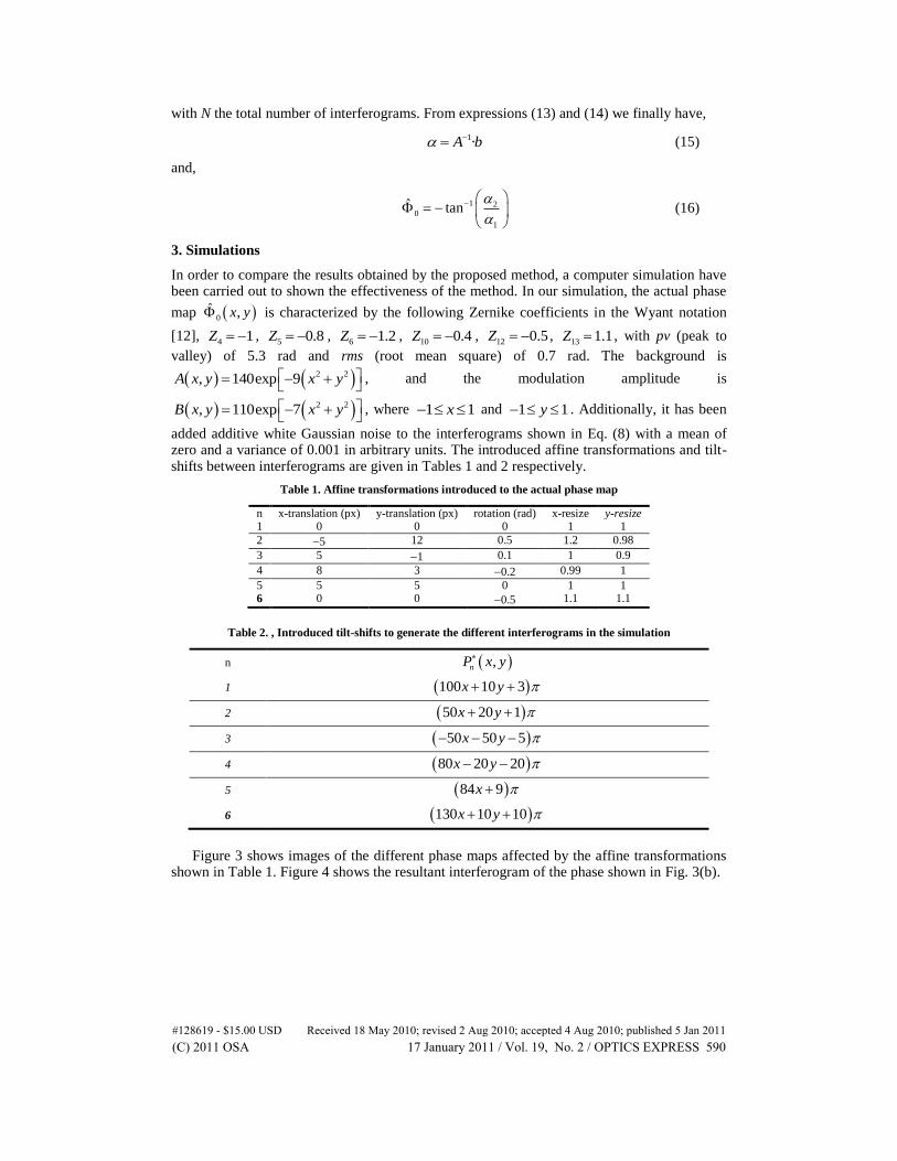
added additive white Gaussian noise to the interferograms shown in Eq. (8) with a mean of zero and a variance of 0.001 in arbitrary units. The introduced affine transformations and tilt-shifts between interferograms are given in Tables 1 and 2 respectively.

Table 1. Affine transformations introduced to the actual phase map

n x-translation (px) y-translation (px) rotation (rad) x-resize y-resize 1 0 0 0 1 1

2 5 12 0.5 1.2 0.98

3 5 1 0.1 1 0.9

4 8 3 0.2 0.99 1

5 5 5 0 1 1 6 0 0 0.5 1.1 1.1

Table 2. , Introduced tilt-shifts to generate the different interferograms in the simulation

n ,nP x y

1 100 10 3x y

2 50 20 1x y

3 50 50 5x y

4 80 20 20x y

5 84 9x

6 130 10 10x y

Figure 3 shows images of the different phase maps affected by the affine transformations shown in Table 1. Figure 4 shows the resultant interferogram of the phase shown in Fig. 3(b).


Fig. 3. Phase map described in the simulation section affected by the affine transformations shown in Table 1

Fig. 4. Resultant interferogram of the phase shown in Fig. 2(b)


In Fig. 5, it is shown the different phases 0 ,n nx y recovered using the Fourier

transform demodulation method and the obtained control points. With these control points the affine transformations between the first interferogram and the rest of them are computed.

Fig. 5. Different phases 0 ,n nx y shown in Fig. 2, recovered using the Fourier transform

demodulation method with the detected control points

In Fig. 6 it is shown the difference between the phases after affine registration process

0 ,x y and the phase corresponding to the first interferogram that is used as reference. As

can be seen from Figs. 6(a), (b), (c), (d) and (e) the affine registration process works correctly and the differences come from the typical ripple artifacts. The rms (root mean square error) of

the difference between the phases after affine rectification 0 ,x y and the phase

corresponding to the first interferogram is shown in Table 3. In Table 3 it is also shown the relative error (err) of the different affine rectificated phases obtained from the division between the computed rms, shown in Table 3, and the pv of the actual phase map that is 5.3 rad. As can be seen from Table 3, the mean of the rms and relative errors are 0.096 rad and 0.28% respectively. After determining the different affine transformations, the different interferograms and tilt-shifts are affine registered with respect to the first one.


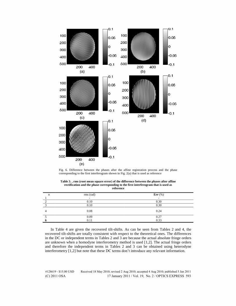
Fig. 6. Difference between the phases after the affine registration process and the phase corresponding to the first interferogram shown in Fig. 2(a) that is used as reference

Table 3. , rms (root mean square error) of the difference between the phases after affine rectification and the phase corresponding to the first interferogram that is used as

reference

n rms (rad) Err (%) 1 - -

2 0.10 0.30

3 0.10 0.30

4 0.08 0.24

5 0.09 0.27 6 0.11 0.33

In Table 4 are given the recovered tilt-shifts. As can be seen from Tables 2 and 4, the recovered tilt-shifts are totally consistent with respect to the theoretical ones. The differences in the DC or independent terms in Tables 2 and 3 are because the actual absolute fringe orders are unknown when a homodyne interferometry method is used [1,2]. The actual fringe orders and therefore the independent terms in Tables 2 and 3 can be obtained using heterodyne interferometry [1,2] but note that these DC terms don’t introduce any relevant information.


Table 4. , Recovered tilt-shifts in the simulation

n ,nP x y

1 100 10 32x y

2 50 20.1 20.7x y

3 50.2 49.5 29.2x y

4 80.1 19.7 17.7x y

5 84.2 0.27 24.7x y

6 129.7 9.2 40x y

Finally, in Fig. 7 it is shown the recovered phase 0 ,x y after the general temporal

demodulation method and in Fig. 8 it is shown the difference between the recovered phase and the theoretical phase. The rms (root mean square error) of the difference between both phases is of about 0.054 rad. As can be seen from Table 3, the rms values obtained from the Fourier transform demodulating method are in all cases larger than the rms error recovered from the temporal demodulation method and using all interferograms.

Fig. 7. Recovered phase 0 ,x y after the general temporal demodulation method


Fig. 8. Difference between the recovered phase and the theoretical phase

4. Experimental results

For further verification of the performance of the proposed algorithm, we have applied it to experimental interferograms. We have used a Mach-Zehnder interferometer where the phase-shifts are introduced by induced vibrations without the need of any phase-shifter device. With this interferometer and using the proposed method we have characterized a high quality λ/100 glass plate. On the other hand the test plate has been also measured by using a commercial Zygo GPI Fizeau phase-shifting interferometer with a vibration-isolating platform. Images of the results obtained by the Zygo and Mach-Zenhder interferometers are shown in Figs. 9 and 10 respectively. As can be seen from Figs. 9 and 10, the general shape of the phase is similar in both cases.

Fig. 9. Results obtained by the Zygo GPI interferometer for the λ/100 high quality glass plate

The obtained rms (root mean square) and pv (peak to valley) of the wave-front error measured by the Zygo interferometer using a four step phase-shifting algorithm and with the Mach-Zenhder interferometer using the proposed method with ten interferograms is shown in Table 5.


Fig. 10. Result obtained by the Mach-Zenhder interferometer using the proposed method for the λ/100 high quality glass plate

Table 5. , rms (root mean square) and pv (peak to valley) of the wave-front error measured by the Zygo interferometer and with the Mach-Zenhder interferometer for the

λ/100 high quality glass plate

rms (waves) pv (waves)

Zygo 0.010 0.068

Mach-Zenhder 0.0091 0.042

As can be seen from Table 5, the results obtained with both instruments are very similar. The difference in the rms measurement is of about 0.0009 waves. On the other hand, the difference in the pv measurement is 0.026 waves.

5. Conclusions

We have proposed an interferometric method that is capable to obtain accurate measures when severe vibrations are present, that it is the case when it is desired to perform an object interferometric characterization inside a thermal-vacuum chamber, for example. The method doesn’t need any phase-shifter device and it takes advantage of these vibrations to produce the different phase-steps that are used to demodulate the phase. The proposed method is based on spatial and time domain processing techniques to compute first the different unknown phase-shifts and then reconstruct the phase from these tilt-shifted interferograms. In order to compensate the camera movement, it is needed to perform an affine registration process between the different interferograms. Simulated results and experiments demonstrate the effectiveness of the proposed method. This method can be used in a very hostile environment as thermo-vacuum chambers to obtain accurate interferometric tests. On the other hand costly phase-shifting devices are not longer required for steady-state measures.


phase-shifting interferometry based on induced vibrationseprints.ucm.es/22321/1/quirogaja15.pdf ·...

Documents