pervaporation using graphene oxide membranesetheses.whiterose.ac.uk/12282/1/pervaporation using...

1

Pervaporation Using Graphene

Oxide Membranes

by

Mindaugas Paulauskas

Submitted in accordance with the requirements for the degree of

Doctor of Philosophy

The University of Leeds

School of Chemistry

December 2015

2

Intellectual Property and Publication Statement

The candidate confirms that the work submitted is his own, except where work which

has formed part of jointly-authored publications has been included. The contribution of

the candidate and the other authors to this work has been explicitly indicated below.

The candidate confirms that appropriate credit has been given within the thesis where

reference has been made to the work of other.

Chapter 4 of this thesis contain theory and results presented by the author at the “2nd

Fluid Flow, Heat and Mass Transfer” conference in Canada 2015.

This copy has been supplied on the understanding that it is copyright material and that

no quotation from the thesis may be published without proper acknowledgement.

2015, The University of Leeds, Mindaugas Paulauskas.

The right of Mindaugas Paulauskas to be identified as Author of this work has been

asserted by him in accordance with the Copyright, Designs and Patents Act 1988.

3

Acknowledgements

This is thesis is one of the main outcomes of my 4 years integrated MSc and Ph.D.

research activities at the University of Leeds in the Institute of the Process Research

and Development (IPRD). During my studies a number of institutions and people have

contributed to my research and I would like to take this opportunity to acknowledge all

their good will. I would especially like to thank:

Professor Frans Muller for giving this great opportunity to join his group and for

sharing his scientific insights during my studies.

Professor Simon Biggs and Dr Charlotte Willans for being my co-supervisor

and making a large contribution for my professional development

Professor Andrew Livingston for agreeing to be my external examiner and

discussing my research.

Professor Peter Heggs for agreeing to be my internal examiner.

The Engineering and Physical Science Research Council (EPSRC) for the

research funding.

Special thanks to everyone working in the IPRD laboratories for their

continuous support and valuable advice.

Croda for giving me an opportunity to do an industrial placement at their

process research site in the Rawcliffe Bridge.

Dr James Birbeck and Dr Richard Cawthorne for overseeing my research in

industry

Dr Rahul Raveendran-Nair for helping to start this research project

Everyone at the Rawcliffe Bridge site working in the R&D laboratories for their

continuous scientific enthusiasm and inspiration.

Mr Stuart Micklethwaite for training me on SEM imaging techniques.

Dr Algy Kazlauciunas for the TGA and DSC work.

Matthew Broadbent for his excellent mechanical engineering work.

MEng student Isadora Rodrigues for a valuable addition to my research work.

Michael Chapman, James McManus, James Coleman and Dr Peter Baldwin for

the thesis proof reading.

Emmanuel Kimuli, Simukai Mashanga, Aminul Hoque, James Coleman, Arjun

Kandola, and Mohammed Ali for their support, advice and friendship throughout

my undergraduate, MSc and Ph.D. studies.

Jana Kautenburger for her unwavering support and good advice at the time of

need.

4

My friends at home Domas Belenavicius, Vaidas Belenavicius, Audrius

Mazonas and Rokas Sidlauskas for their warm welcome during my trips to

Lithuania.

My family Robertas Paulauskas, Loreta Paulauskiene, Ugne Paulauskaite,

Liudas Rudys and Irena Rudiene for their unwavering support throughout my

undergraduate, MSc and Ph.D. studies.

5

“Lack of comfort means we are on the threshold of new insights.”

Lawrence M. Krauss (1954, American Theoretical Physicist and Cosmologist)

http://www.goodreads.com/author/show/1410.Lawrence_M_Krauss

6

Abstract

Pervaporation is a perspective fluid separation technology. Membranes are widely

recognised for their energy and capital cost savings. Currently, most of the research is

focused on developing new membrane material that are stable in a wide range of

temperatures in a presence of organic solvents. This research is focused on a graphene

oxide, a novel and highly selective membrane material. Graphene oxide has attracted a

lot of academic research attention. Many researchers have demonstrated selective water

removal using this material, however moving forward the data lack the scope and depth

of understanding of the material performance at different process conditions and fluid

systems.

Previous research has not addressed graphene oxide stability and performance in a wide

range of conditions which are crucial for assessing the material’s potential as a water

selective membrane material for industrial applications. The purpose of this work is to

investigate graphene oxide membrane pervaporation permeation flux and selectivity

using common aqueous organic solvent solutions. Three industrial case studies are also

investigated to determine whether the material is ready to be applied on a larger scale

and has a potential to replace distillation. Previous research has also missed graphene

oxide low price advantage, which stems from the cheap starting materials. This has been

brought up and discussed in the final results chapter of the thesis.

The key outcome of this research is a demonstration of the graphene oxide

pervaporation flux drop at elevated temperatures and the behaviour deviation from the

solution-diffusion model. The membrane has also been rapidly fouled when exposed to

aqueous peptide solutions. This research brings a large amount of experimental and

analytical data, which points in a direction of the research avenues to be pursued in order

to improve graphene oxide as a selective membrane material.

7

Table of Contents

1 Introduction ......................................................................................................... 25

1.1 Research Strategy and Motivation ................................................................ 27

1.2 Membrane Materials ..................................................................................... 30

1.2.1 Polymeric Membrane ............................................................................. 31

1.2.2 Inorganic membranes ............................................................................ 34

1.2.3 Mixed matrix and hybrid materials ......................................................... 36

1.3 Industrial use of pervaporation ...................................................................... 39

1.4 G.O. a selective membrane material ............................................................. 42

1.4.1 Membrane manufacturing ...................................................................... 45

1.4.2 Brodie’s Method ..................................................................................... 46

1.4.3 Hummers Method .................................................................................. 46

1.4.4 Improved Hummers method .................................................................. 46

1.4.5 Coating .................................................................................................. 47

1.5 G.O. Membranes Selective Water Separations............................................. 48

1.5.1 Polymer supported and free standing G.O. membranes ........................ 48

1.5.2 Ceramic Supported Graphene Oxide ..................................................... 55

1.6 Summary of Pervaporation Membranes ........................................................ 56

2 Pervaporation Modelling ..................................................................................... 58

2.1 Pore-flow model ............................................................................................ 59

2.2 Solution-diffusion model ............................................................................... 64

2.3 Concentration polarisation ............................................................................ 68

8

2.3.1 Liquid and membrane layer concentration polarization .......................... 72

2.3.2 Desorption of water at the membrane/support interface and diffusion

through the porous support ................................................................................. 75

2.3.3 Transport through the vapour boundary layer ........................................ 76

2.3.4 Combined mass transfer model ............................................................. 76

3 Methods and Materials ........................................................................................ 78

3.1 Membrane Coating ....................................................................................... 78

3.2 Pervaporation Cell ........................................................................................ 79

3.3 General Procedure ....................................................................................... 82

3.4 Liquid side mass transfer coefficient study .................................................... 87

3.5 Water/Organic and Organic/Organic separations .......................................... 87

3.6 Peptide dewatering ....................................................................................... 89

3.7 Esterification ................................................................................................. 90

3.8 Material characterisation ............................................................................... 90

3.8.1 FT-IR ..................................................................................................... 90

3.8.2 Thermal Properties ................................................................................ 91

3.8.3 SEM and EDX ....................................................................................... 91

3.8.4 Contact Angle ........................................................................................ 91

3.9 Water Analysis .............................................................................................. 92

3.9.1 Karl Fischer analysis ............................................................................. 92

3.9.2 GC analysis ........................................................................................... 92

3.9.3 Refractometer ........................................................................................ 92

4 Organic Solvent Dehydration .............................................................................. 93

9

4.1 Experimental setup validation ....................................................................... 93

4.2 G.O. membrane long term performance ....................................................... 98

4.3 Visual analysis .............................................................................................. 99

4.4 Thermal degradation................................................................................... 101

4.5 XRD analysis .............................................................................................. 103

4.6 FT-IR analysis ............................................................................................ 105

4.7 Solution-diffusion model validation .............................................................. 108

4.7.1 Temperature effects ............................................................................ 108

4.7.2 Membrane thickness ........................................................................... 111

4.7.3 Water concentration effects ................................................................. 112

4.8 Summary .................................................................................................... 114

5 Industrial Case Studies ..................................................................................... 115

5.1 Organic/Organic Separation ....................................................................... 115

5.2 Esterification ............................................................................................... 117

5.3 Peptides ..................................................................................................... 126

5.3.1 Peptide 1 Hydrolysate.......................................................................... 126



6 Process Modelling and Economics .................................................................... 138

6.1 Process ...................................................................................................... 139

6.2 Simulation method ...................................................................................... 140

6.3 Energy Consumption Modelling-Distillation ................................................. 143

10

7 Pervaporation separation of Water/IPA mixtures ............................................... 147

7.1 Process ...................................................................................................... 147

7.2 Simulation methodology and process energy requirement .......................... 148

7.3 Economic assessment ................................................................................ 151

7.4 Pervaporation and distillation energy consumption ..................................... 151

7.5 Membrane surface area requirements and cost .......................................... 152

8 Conclusions and Future Research .................................................................... 159

8.1 Conclusions ................................................................................................ 159

8.2 Future Research ......................................................................................... 161

9 Appendix ........................................................................................................... 163

9.1 Appendix A Experimental Data ................................................................... 163

9.2 Appendix B Detailed Distillation Process Information .................................. 174

9.3 Appendix C Detailed Pervaporation Cell Drawings ..................................... 175

9.4 Appendix D Standard Operating Procedure ................................................ 178

10 Reference ......................................................................................................... 182

11

List of Figures

Figure 1 - Membrane classification based on the nominal pore sizes (Membrane

technology and applications) ...................................................................................... 26

Figure 2 – Research Progress Flow Chart .................................................................. 29

Figure 3-Precursors used for the HybSi membrane .................................................... 36

Figure 4 – a) Conventional ethyl acetate production, b) membrane assisted ethyl acetate

production ................................................................................................................... 41

Figure 5 - Membrane reactor ...................................................................................... 42

Figure 6 –Variation of the Left-Klinowski G.O. model [57] ........................................... 43

Figure 7 – Simplistic representation of a G.O. membrane stacking and potential water

entrance points[3] ....................................................................................................... 44

Figure 8 – Overview of the G.O. membrane production process ................................. 45

Figure 9 – Typical three piece vacuum filter ................................................................ 47

Figure 10 – Permeation experiments a) gas experiment setup b) water experiment

setup[1] ....................................................................................................................... 49

Figure 11 – Dip coating procedure. ............................................................................. 54

Figure 12-Aqueous ethanol mixture dehydration using different membranes .............. 57

Figure 13-Pore-flow model a) depiction of the core concepts, b) schematic representation

of the model.[2, 77] ..................................................................................................... 60

Figure 14 – Pore-flow model predictions of permeate water mole fraction[77] ............ 64

Figure 15 – Schematics of the solution diffusion concepts[2] ...................................... 65

Figure 16 – Detailed resistance in series model .......................................................... 69

Figure 17 - Concentration polarization [83] ................................................................. 72

12

Figure 18-Concentration Polarization with respect to 𝑁 value[91] ............................... 75

Figure 19 Pervaporation cell computer design ............................................................ 80

Figure 20 – Pervaporation cell disassembled view ...................................................... 81

Figure 21 – Detailed pervaporation process drawing .................................................. 85

Figure 22 – Laboratory pervaporation setup ............................................................... 86

Figure 23-Pervaporation flux change with respect to the change in agitation, water/IPA

(30 / 70wt%), 50°C, 2.1μm. ......................................................................................... 94

Figure 24- Mass transfer resistance (%) change with respect to the change in membrane

thickness, water/IPA (30 / 70wt%), 50°C, 2.1 – 0.01μm .............................................. 97

Figure 25-Membrane stability over 7 day period, water/IPA (20 / 80wt%), 80°C, 2.1μm.

................................................................................................................................... 98

Figure 26-Membrane stability over 7 day period (percent permeation flux values),

water/IPA (20 / 80wt%), 80°C, 2.1μm. ........................................................................ 99

Figure 27-DSC scan in a 0-500°C temperature range at a 5°C per minute heating rate

................................................................................................................................. 101

Figure 28-TGA scan in a 0-500°C temperature range at a 5°C per minute heating rate

................................................................................................................................. 101

Figure 29-XRD patterns of i) Graphite, ii) PVDF, iii) New Membrane, and iv) G.O.

membrane tested in a 7 day pervaporation process. ................................................. 104

Figure 30-XRD patterns of i) Graphite, ii) PVDF, and iii) G.O. Membrane (1 µm) ...... 104

Figure 31- FT-IR of G.O. ........................................................................................... 105

Figure 32-FT-IR of i) G.O, ii) Used Membrane, iii) New Membrane, and iv) PVDF .... 106

Figure 33-FT-IR spectra of i) G.O., ii) Soaked Membrane, and iii) Used Membrane . 107

13

Figure 34 – Water contact angle on the a) fresh G.O. membrane, and b) used G.O.

membrane ................................................................................................................ 107

Figure 35-Pervaporation flux of water/IPA (30 / 70wt%) solution at 50, 60, and 70°C,

2.1μm membrane ..................................................................................................... 109

Figure 36-Pervaporation of water/ethanol (30 / 70wt%) solution at 50, 60, 70, 80°C, 2.1

µm membrane .......................................................................................................... 110

Figure 37-Pervaporation of water/THF (30 / 70wt%) solution at 50, 60, 70°C, 1.0 µm

membrane ................................................................................................................ 110

Figure 38-Pervaporation of water/IPA (30 / 70wt%) vs inverted membrane thickness

(0.56, 1 and 2.1μm), 50 and 60°C ............................................................................. 111

Figure 39-Pervaporation flux with respect to the water concentration, water/IPA (1 –

100wt%), 50°C, 2.1μm membrane ............................................................................ 112

Figure 40-Pervaporation flux vs mole fraction corrected driving force, water/IPA (1 –

100wt%), 50°C, 2.1μm membrane ............................................................................ 113

Figure 41-Membrane Comparison ............................................................................ 114

Figure 42-Pervaporation flux of MeOH/n-Hexane (5 – 55wt%), 60°C, 2.1μm membrane

................................................................................................................................. 116

Figure 43-Pervaporation assisted esterification reaction setup ................................. 118

Figure 44-Effects of selective water removal on esterification reaction conversion, 100°C,

2.1μm membrane ..................................................................................................... 120

Figure 45-Pervaporation flux and permeate purity vs time, 100°C, 2.1μm membrane

................................................................................................................................. 120

Figure 46-Pervaporation flux change vs water wt% in the reaction mixture, 100°C, 2.1μm

membrane ................................................................................................................ 121

14

Figure 47-Energy dispersive X-ray spectroscopy characterisation of the G.O. membrane

exposed to an esterification reaction ......................................................................... 123

Figure 48-FT-IR spectrum of used (esterification reaction, 100°C, 2.1μm membrane) and

fresh G.O. membrane ............................................................................................... 124

Figure 49 - Water contact angle on the a) fresh G.O. membrane, and b) used G.O.

membrane in an esterification reaction ..................................................................... 125

Figure 50-Pervaporation of aqueous Peptide 1 Hydrolysate (2 – 8wt% solids) at 80°C,

2.1 µm membrane .................................................................................................... 128

Figure 51-Pervaporation of aqueous Peptide 2 Hydrolysate (5wt% solids) at 80°C, 2.1

µm membrane .......................................................................................................... 129

Figure 52-Pervaporation of aqueous Peptide 3 (2wt% solids) solution at 70°C, 2.1 µm

membrane ................................................................................................................ 130

Figure 53-SEM images of membranes used in i) Peptide 1 hydrolysate, ii) Peptide 3, and

iii) Peptide 2 peptide dewatering processes .............................................................. 133

Figure 54-EDX spectrum of a membrane used in a Peptide 1 peptide dewatering process

................................................................................................................................. 134


................................................................................................................................. 135


(scan1) ..................................................................................................................... 136

Figure 57 – Water contact angles of a) Unused membrane, b) Peptide 3 peptide exposed

membrane, and c) Peptide 2 peptide exposed membrane ........................................ 137

Figure 58 - x-y diagram of IPA and water[125] .......................................................... 139

Figure 59-Conventional extractive distillation ............................................................ 140

Figure 60 – Mass flow balance on a single stage ...................................................... 141

15

Figure 61-Extractive distillation of the IPA ................................................................. 144

Figure 62 - Composition profiles in the extractive column ......................................... 145

Figure 63 - Composition profiles in the entrainer recovery column ............................ 146

Figure 64 – Pervaporation energy requirement simulation ........................................ 150

Figure 65 – Pervaporation module surface area estimation program ........................ 154

Figure 66 –Simulated pervaporation cell model[141] ................................................ 155

Figure 67-Single block of a simulated pervaporation cell[141]................................... 155

Figure 68-Required membrane surface area vs different degrees of dryness for 1000

kg/h 30wt% water in IPA using 2.1 µm G.O. membrane at 70°C ............................... 157

Figure 69-Pervaporation cell process side drawing ................................................... 175

Figure 70 – Pervaporation cell process side drawing ................................................ 175

Figure 71 - Pervaporation cell membrane saddle drawing ........................................ 176

Figure 72 - Pervaporation cell membrane saddle drawing ........................................ 176

Figure 73-Porous stainless steel support drawing ..................................................... 177

Figure 74 –Stainless steel support drawing ............................................................... 177

16

List of Tables

Table 1 –Dehydration of alcohols using polymeric membranes [23, 30, 31] ................ 33

Table 2-Dehydration of alcohols using inorganic membranes ..................................... 35

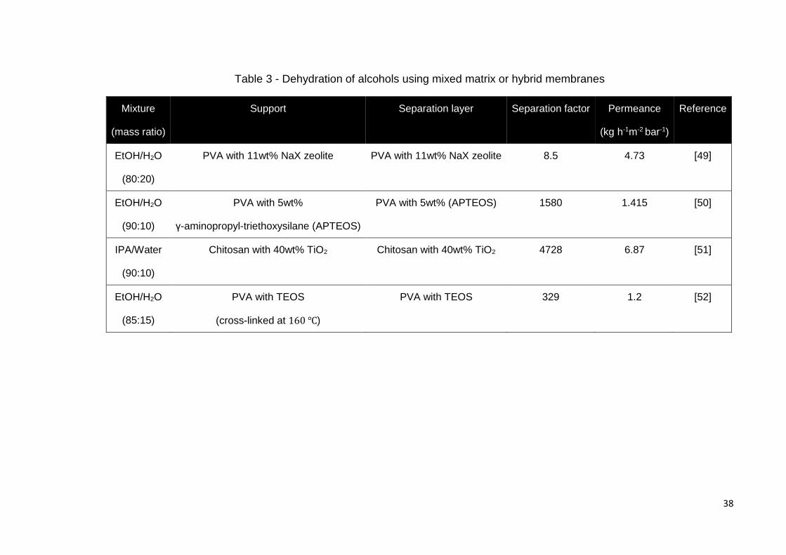
Table 3 - Dehydration of alcohols using mixed matrix or hybrid membranes ............... 38

Table 4-Summary of fluid permeation experiments at room temperature [1] ............... 50

Table 5-Water permeation through G.O. (PTFE support) ............................................ 50

Table 6-Water permeation through G.O. (hydrophilic support) [16] ............................. 51

Table 7-Organic compound dehydration using G.O. membrane. ................................ 53

Table 8-EtOH dehydration using G.O. membrane at a room temperature.[17] ............ 54

Table 9-EtOH dehydration using G.O. membrane at 77°C.[15] ................................... 55

Table 10-DMC dehydration using G.O. membrane.[75] .............................................. 56

Table 11-Antoine constants for water in the temperature range 273-303 K [84] .......... 68

Table 12-Vapour transport in porous media ................................................................ 76

Table 13-Pervaporation cell component list ................................................................ 81

Table 14-Energy required to evaporate 2.69g of water over 60min of operation ......... 83

Table 15-Heat transfer rate from hot oil bath the pervaporation cell ............................ 83

Table 16-Summary of the heat requirements in a pervaporation process ................... 84

Table 17-Summary of the Water/Organic and Organic/Organic separations ............... 88

Table 18-Materials used in the research ..................................................................... 88

Table 19-Materials used in the peptide dewatering process ........................................ 89

Table 20-Summary of the peptide dewatering experiments ........................................ 89

Table 21- Mass transfer coefficients, water/IPA (30 / 70wt%), 50°C, 2.1μm. ............... 96

17

Table 22 - Visual G.O. Characterisation .................................................................... 100

Table 23-MeOH pervaporation flux and permeate purity and different temperatures 116

Table 24-Visual G.O. membrane characterisation ..................................................... 122

Table 25-Estimates of membrane areas required to replace current evaporator process

................................................................................................................................. 126

Table 26-Unused G.O. membrane SEM images ....................................................... 131

Table 27-Selected case study design specifications ................................................. 138

Table 28-NRTL Parameters from Aspen Plus Properties Database .......................... 142

Table 29-Energy consumption of azeotropic distillation process ............................... 146

Table 30-Energy consumption of a membrane separation process ........................... 151

Table 31-Pervaporation and distillation energy requirements .................................... 152

Table 32-Lab scale costs of the G.O. membrane production .................................... 158

Table 33-Raw material prices used in the G.O. synthesis ......................................... 158

Table 34-Water/IPA (20wt%/80wt%) 7 day dewatering study, 80°C, 2.1 µm membrane

................................................................................................................................. 163

Table 35-Water/IPA (30wt% / 70wt%) varying temperature (50-70°C) study, 2.1 µm

membrane ................................................................................................................ 164

Table 36-Water / EtOH (30wt% / 70wt%) varying temperature (50-80°C) study, 2.1 µm

membrane ................................................................................................................ 165

Table 37-Water / THF (30wt% / 70wt%) varying temperature (50-70°C) study, 1 µm

membrane ................................................................................................................ 165

Table 38-Water/IPA (30-5wt%) permeation study, 2.1µm, 50°C ............................... 166

Table 39-Water/IPA (12.5-8wt%) permeation study, 2.1µm, 50°C ............................. 166

18

Table 40-Water/IPA (5-4wt%, and 1wt%) permeation study, 2.1µm, 50°C ................ 167

Table 41-Water/IPA (30 / 70wt%) Liquid side mass transfer coefficient study1, 2.1µm,

50°C ......................................................................................................................... 167


50°C ......................................................................................................................... 167


50°C ......................................................................................................................... 168

Table 44-MeOH / n-Hexane pervaporation study, 2.1µm .......................................... 169

Table 45-IPA and carboxylic acid esterification study1, 100°C, 2.1µm, 03.02.2015 .. 170



Table 48-Peptide 2 peptide dewatering study (5wt% solids), 80°C, 2.1µm ................ 172

Table 49-Peptide 1 peptide dewatering study (2-8wt% solids), 80°C, 2.1µm ............ 172

Table 50-Peptide 3 peptide dewatering study (2wt% solids), 70°C, 2.1µm, 07.01.2015

................................................................................................................................. 173

19

Abbreviations

Abbreviation Meaning

CRC Scheme Carbon Reduction Commitment Energy

Efficiency Scheme

BTSE Bis(triethoxysilyl)ethane

DSC Differential Scanning Calorimetry

DMF Dimethylformamide

DMSO Dimethyl sulfoxide

DMC Dimethyl carbonate

EDX Energy Dispersive X-ray

EtOH Ethanol

FT-IR Fourier Transform Infrared

GC Gas Chromatography

G.O. Graphene Oxide

GE Gelatin

IPA 2-propanol

MTES Methyltriethoxysilane

MeOH Methanol

NRTL Non-Random Two Liquid (model)

NMP N-Methyl-2-pyrrolidone

PI Process Intensification

PTFE Polytetrafluoroethylene

PVA Polyvinyl alcohol

PVDF Polyvinylidene fluoride

RPM Rotations per Minute

SEM Scanning Electron Microscopy

TEOS Tetraethyl orthosilicate

THF Tetrahydrofuran

TGA Thermogravimetric Analysis

20

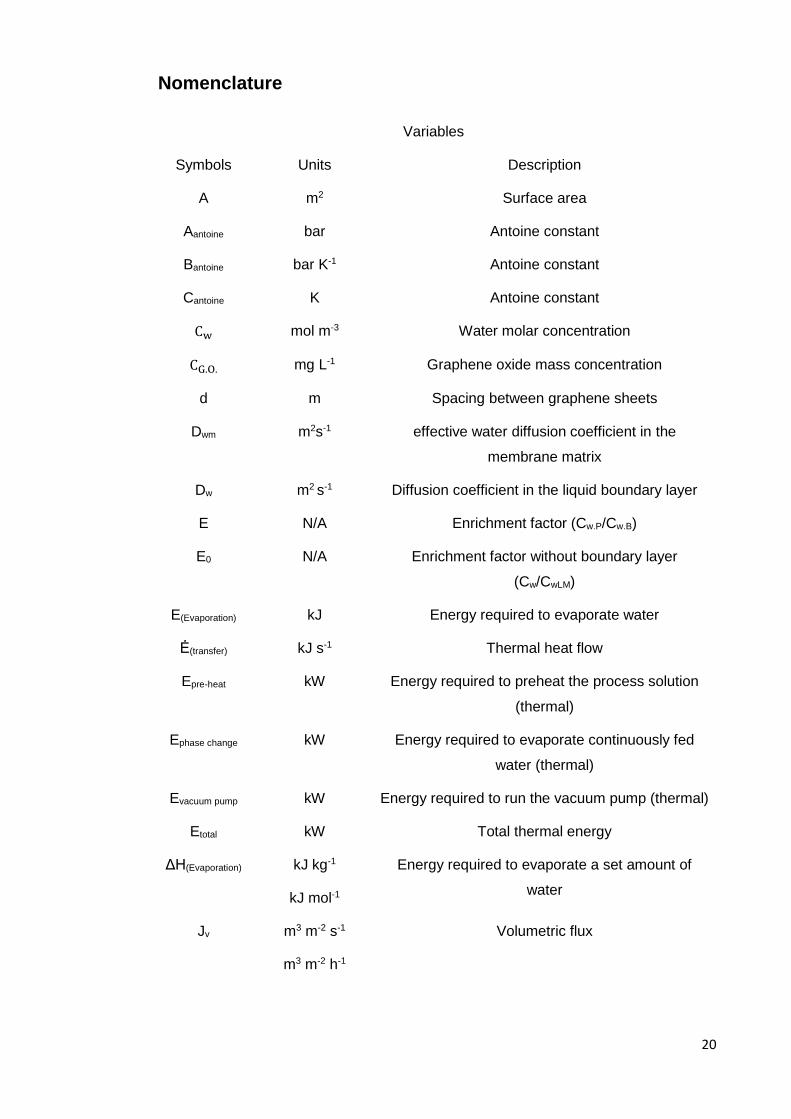
Nomenclature

Variables

Symbols Units Description

A m2 Surface area

Aantoine bar Antoine constant

Bantoine bar K-1 Antoine constant

Cantoine K Antoine constant

Cw mol m-3 Water molar concentration

CG.O. mg L-1 Graphene oxide mass concentration

d m Spacing between graphene sheets

Dwm m2s-1 effective water diffusion coefficient in the

membrane matrix

Dw m2 s-1 Diffusion coefficient in the liquid boundary layer

E N/A Enrichment factor (Cw.P/Cw.B)

E0 N/A Enrichment factor without boundary layer

(Cw/CwLM)

E(Evaporation) kJ Energy required to evaporate water

Ė(transfer) kJ s-1 Thermal heat flow

Epre-heat kW Energy required to preheat the process solution

(thermal)

Ephase change kW Energy required to evaporate continuously fed

water (thermal)

Evacuum pump kW Energy required to run the vacuum pump (thermal)

Etotal kW Total thermal energy

ΔH(Evaporation) kJ kg-1

kJ mol-1

Energy required to evaporate a set amount of

water

Jv m3 m-2 s-1

m3 m-2 h-1

Volumetric flux

21

J kg m-2 s-1

kg m-2 h-1

Mass flux

km kg m2 s-1 bar-1

mol m2 s-1 bar-1

Pressure normalised membrane mass transfer

coefficient

k´m m s-1 Pressure normalised membrane mass transfer

coefficient

kL.P.G.O. kg m m2 s-1 bar-

1

Pressure and membrane thickness normalised

mass transfer coefficient

kM.P. kg m-2 s-1 bar-1

kg m-2 h-1 bar-1

Pressure normalised membrane mass transfer

coefficient

k’H mol m-3 bar-1 Product of the weight of the membrane / volume of

adsorbed gas molecules and Henry’s constant

k`ov m s-1 Overall mass transfer coefficient

k´LM m s-1 Liquid/membrane mass transfer coefficient

KSL N/A Liquid side partition coefficient

𝜌𝑤,𝑀𝐿 = 𝐾𝑆𝐿𝜌𝑤,𝐿𝑀

(can also be used with molar concentrations)

KSG mol bar-1m-3

kg bar-1m-3

Membrane side partition coefficient

𝜌𝑤,𝑀𝑆 = 𝐾𝑆𝐺𝑃𝑤.𝑝

K N/A Adjustable parameter

k´L m s-1 Liquid mass transfer coefficient

m kg, g, mg Mass of the collected permeate sample

Mi kg mol-1 Molecular weight of the component

Nt m-2 Total number of pores per effective area

nf mol s-1 Overall mole flow velocity

npermeate mol s-1 Permeate mole flow velocity

Patmospheric bar Atmospheric pressure

Ppermeate bar Permeate pressure

22

Pprocess bar Process pressure

P* bar Saturated water vapour pressure

P bar Pressure drop

P1 bar Pressure at the start of the pore

P2 bar Pressure at the end of the pore

PW.L bar is the partial vapour pressure of water in

equilibrium with the feed liquid

Pw.P bar Water vapour partial pressure in the permeate

Qliquid mol m-2 s-1 Molar liquid flux

Qvapour mol m-2 s-1 Vapour molar flux

Qsurface mol m-2 s-1 Vapour molar flux across the surface of the pore

Qw.vapour mol m-2 s-1 Water vapour molar flux

Qorg.vapour mol m-2 s-1 Organic compound vapour molar flux

QTotal mol m-2 s-1 Total molar flux

R bar m3 K-1 mol-1 Ideal gas constant, 8.31445*10-5

Rtotal s m-1 Total mass transport resistance

Rliquid s m-1 Liquid phase mass transfer resistance

Rmembrane s m-1 Membrane mass transfer resistance

Rsupport s m-1 Membrane support mass transfer resistance

r m Mean pore diameter

Tperm K Permeate temperature

t s, min, h Time, units of time are noted in calculations

ta m Thickness of the adsorbed gas layer onto a

membrane

T K Temperature

U(Overall) kW m-2K-1 Overall heat transfer coefficient, Assumed

u m s-1 Liquid velocity

VG.O. L Volume of the graphene oxide solution

23

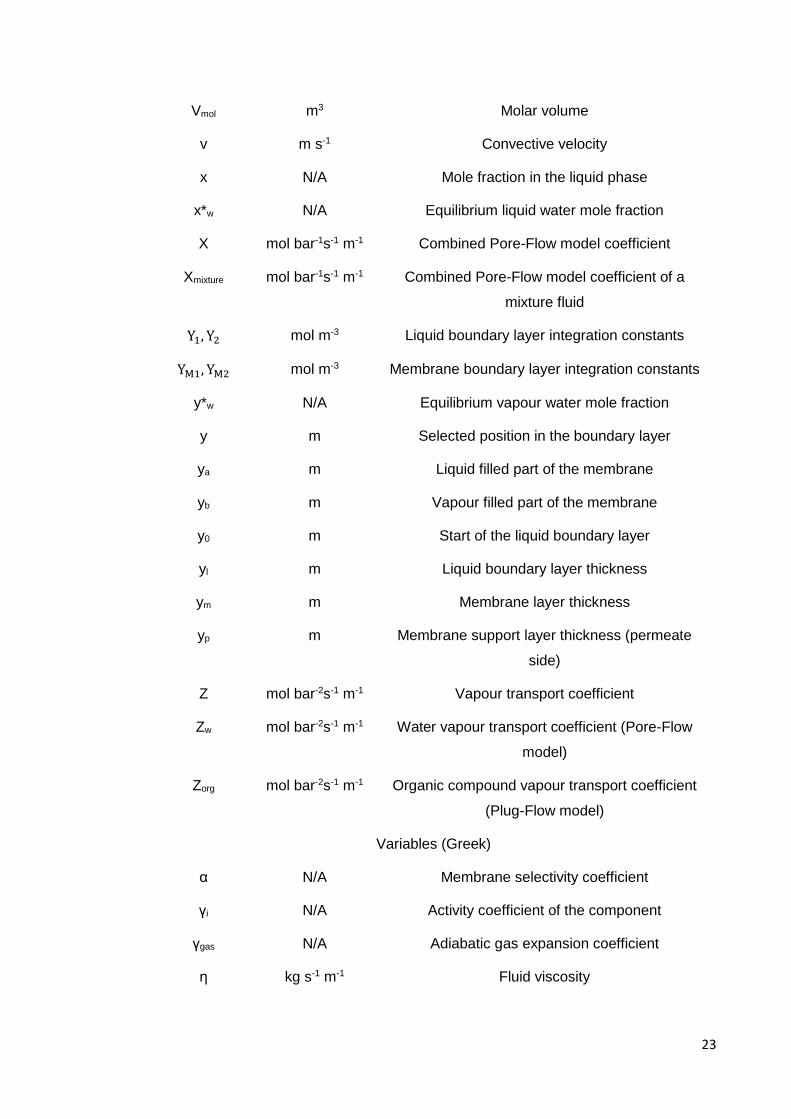
Vmol m3 Molar volume

v m s-1 Convective velocity

x N/A Mole fraction in the liquid phase

x*w N/A Equilibrium liquid water mole fraction

X mol bar-1s-1 m-1 Combined Pore-Flow model coefficient

Xmixture mol bar-1s-1 m-1 Combined Pore-Flow model coefficient of a

mixture fluid

Y1, Y2 mol m-3 Liquid boundary layer integration constants

YM1, YM2 mol m-3 Membrane boundary layer integration constants

y*w N/A Equilibrium vapour water mole fraction

y m Selected position in the boundary layer

ya m Liquid filled part of the membrane

yb m Vapour filled part of the membrane

y0 m Start of the liquid boundary layer

yl m Liquid boundary layer thickness

ym m Membrane layer thickness

yp m Membrane support layer thickness (permeate

side)

Z mol bar-2s-1 m-1 Vapour transport coefficient

Zw mol bar-2s-1 m-1 Water vapour transport coefficient (Pore-Flow

model)

Zorg mol bar-2s-1 m-1 Organic compound vapour transport coefficient

(Plug-Flow model)

Variables (Greek)

α N/A Membrane selectivity coefficient

γi N/A Activity coefficient of the component

γgas N/A Adiabatic gas expansion coefficient

η kg s-1 m-1 Fluid viscosity

24

ηG kg s-1 m-1 Adsorbed gas onto a surface viscosity

ηvac N/A Vacuum pump efficiency

Θ ° X-ray angle

λ N/A Auxiliary function coefficient

λl m Wavelength

μ J mol-1 Chemical potential

ρ kg m-3 Liquid density

ρ𝑤L kg m-3 Water mass concentration in the liquid

χ N/A Membrane tortuosity

Variables (Superscripts)

G Gas

L Liquid

Variables (subscripts)

B Bulk

i Component “i”

P Permeate

SM Support/membrane interface

ML Membrane/liquid interface

LM Liquid/membrane interface

MS Membrane/support interface

W water

Org Organic component

Dimensionless groups and their definitions

NKN σS

dp Knudsen number

Pe Jv yl

Dw

Peclet number

25

1 Introduction

An increase in the global temperature and dwindling fossil fuels over the last several

decades have led to the introduction of a new government legislation to combat the

depletion of these valuable resources.[4] In the UK, the “Carbon Reduction Commitment

Energy Efficiency Scheme” also known as the “CRC Scheme” was designed to improve

energy efficiency in large public and private sector organisations. The main target of the

scheme is to achieve 80% reduction in UK carbon emissions by 2050.[5] This has fuelled

engineering research to focus on the development of more sustainable chemical

processes.

Process intensification (PI) is a common strategy used in the chemical manufacturing

industry to reduce energy usage.[6] One of the aims of PI is to increase the efficiency

and competitiveness of a process. Another aim is to create a faster and more

environmentally friendly processing variant by implementing or designing new

technology.[7] Membrane driven separation processes match the target criteria set out

by the PI principles and have been shown to result in significant energy and capital cost

savings when compared to their counterpart chemical process unit operations.[7, 8] The

advantages of membrane separations made legislator bodies recognise it as the best

available technology (BAT).[9] The main applications of membrane processes typically

involve separation of: gas mixtures, oil/water treatment, separation of organic/organic

and organic/water mixtures.[10]

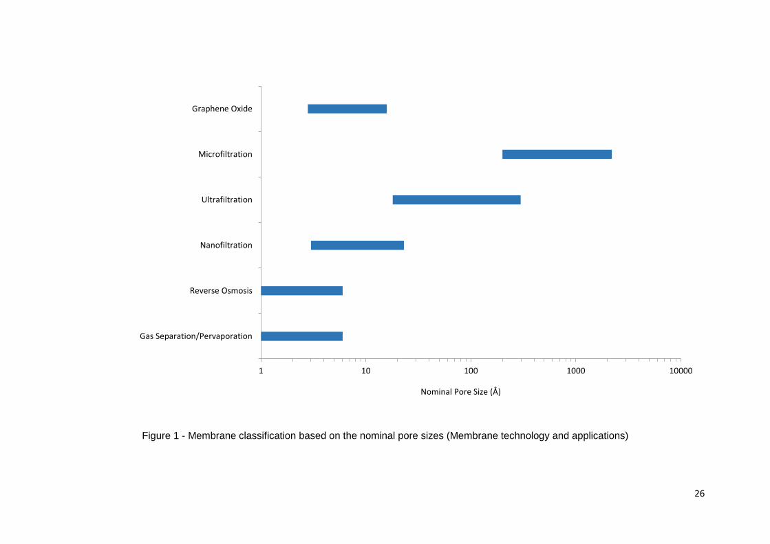
Membranes are categorised based on their nominal pore sizes. Classification of common

membrane groupings is shown in Figure 1. Microfiltration, ultrafiltration and reverse

osmosis membrane processes are well established with many different applications.

Membranes in these categories are provided by multiple experienced companies.[11]

Microfiltration separates small colloidal particles and bacteria within a range of

0.1-10 µm in diameter. Ultrafiltration pore size is tailored to separate dissolved

macromolecules such as proteins. Reverse osmosis is mainly focused on desalination

of brackish water.[12] Pervaporation/Gas separation is the most recent membrane

separation category. Numerous plants are being installed worldwide, the market size is

expanding and process innovations are being made.[11] Pervaporation is considered as

the main technology which has potential to replace azeotropic distillation process.[11,

13] Currently, pervaporation research is focused on novel membrane materials, which

exhibit high permeate selectivity and high permeate fluxes.[14]

26

Figure 1 - Membrane classification based on the nominal pore sizes (Membrane technology and applications)

1 10 100 1000 10000

Gas Separation/Pervaporation

Reverse Osmosis

Nanofiltration

Ultrafiltration

Microfiltration

Graphene Oxide

Nominal Pore Size (Å)

27

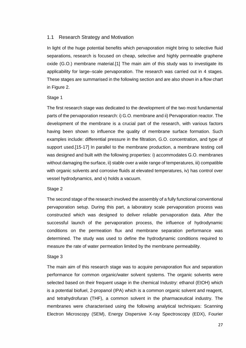
1.1 Research Strategy and Motivation

In light of the huge potential benefits which pervaporation might bring to selective fluid

separations, research is focused on cheap, selective and highly permeable graphene

oxide (G.O.) membrane material.[1] The main aim of this study was to investigate its

applicability for large–scale pervaporation. The research was carried out in 4 stages.

These stages are summarised in the following section and are also shown in a flow chart

in Figure 2.

Stage 1

The first research stage was dedicated to the development of the two most fundamental

parts of the pervaporation research: i) G.O. membrane and ii) Pervaporation reactor. The

development of the membrane is a crucial part of the research, with various factors

having been shown to influence the quality of membrane surface formation. Such

examples include: differential pressure in the filtration, G.O. concentration, and type of

support used.[15-17] In parallel to the membrane production, a membrane testing cell

was designed and built with the following properties: i) accommodates G.O. membranes

without damaging the surface, ii) stable over a wide range of temperatures, iii) compatible

with organic solvents and corrosive fluids at elevated temperatures, iv) has control over

vessel hydrodynamics, and v) holds a vacuum.

Stage 2

The second stage of the research involved the assembly of a fully functional conventional

pervaporation setup. During this part, a laboratory scale pervaporation process was

constructed which was designed to deliver reliable pervaporation data. After the

successful launch of the pervaporation process, the influence of hydrodynamic

conditions on the permeation flux and membrane separation performance was

determined. The study was used to define the hydrodynamic conditions required to

measure the rate of water permeation limited by the membrane permeability.

Stage 3

The main aim of this research stage was to acquire pervaporation flux and separation

performance for common organic/water solvent systems. The organic solvents were

selected based on their frequent usage in the chemical Industry: ethanol (EtOH) which

is a potential biofuel, 2-propanol (IPA) which is a common organic solvent and reagent,

and tetrahydrofuran (THF), a common solvent in the pharmaceutical industry. The

membranes were characterised using the following analytical techniques: Scanning

Electron Microscopy (SEM), Energy Dispersive X-ray Spectroscopy (EDX), Fourier

28

Transform Infrared (FT-IR), Differential Scanning Calorimetry (DSC), Thermal

Gravimetric Analysis (TGA), X–ray Diffraction (XRD), and surface contact angle

measurements.

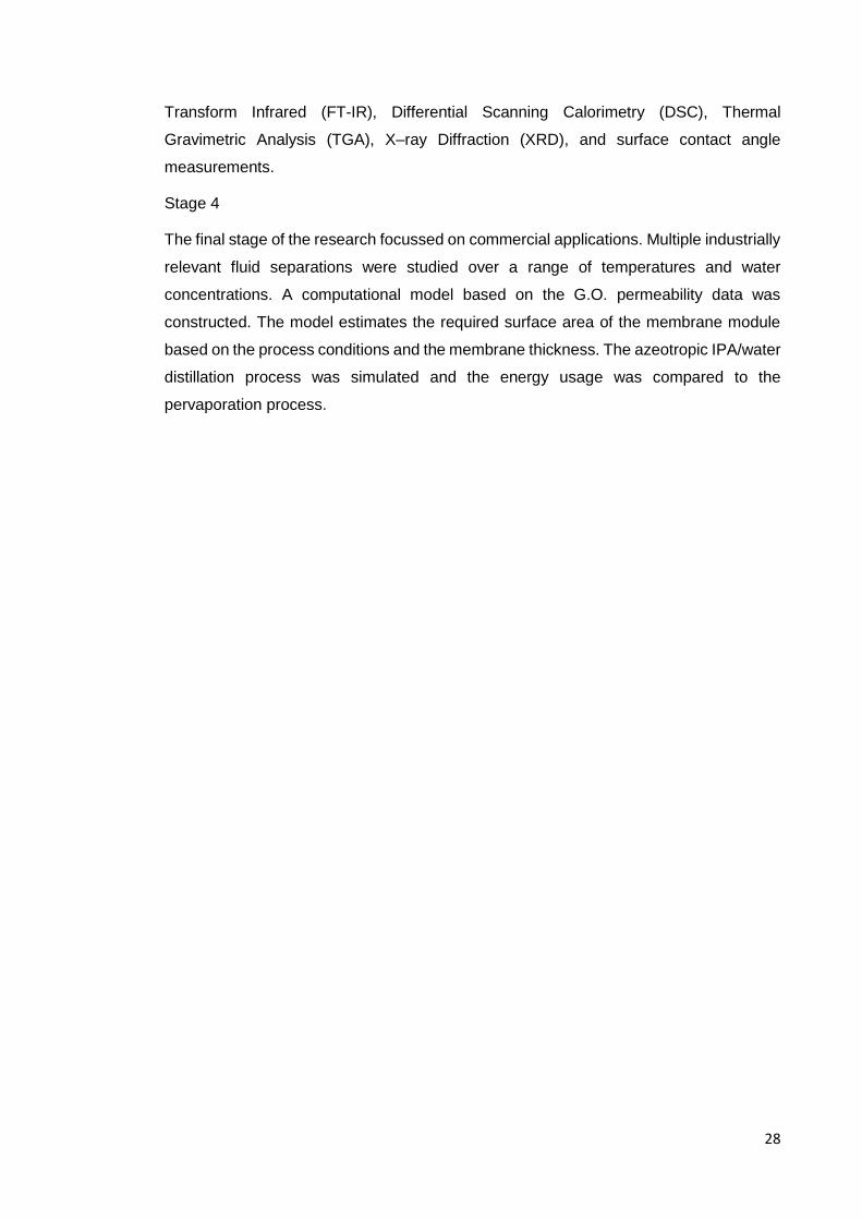
Stage 4

The final stage of the research focussed on commercial applications. Multiple industrially

relevant fluid separations were studied over a range of temperatures and water

concentrations. A computational model based on the G.O. permeability data was

constructed. The model estimates the required surface area of the membrane module

based on the process conditions and the membrane thickness. The azeotropic IPA/water

distillation process was simulated and the energy usage was compared to the

pervaporation process.

29

Pervaporation Cell

Design

Membrane

Production

Pervaporation

Process Design

Pervaporation Test

Validation

Model Solution Tests

Membrane

Characterisation

Industrial Case

Studies

Membrane

Characterisation

Research Progress

Stage

1 2 3 4

Figure 2 – Research Progress Flow Chart

30

1.2 Membrane Materials

Currently, research is concentrated on membrane development with the aim of improving

(i) material's resistance to various solvents (THF, N-methyl-2-pyrrolidone (NMP)), ii)

material's resistance to acid, (iii) mechanical strength, (iv) pervaporation flux and (v)

separation selectivity.[14, 18, 19] To objectively compare membrane performance in the

literature review several key concepts have to be defined. Typically, pervaporation data

is presented in a form of flux, which is a product of a pervaporation constant and a driving

force, .Equation 1. In the pervaporation flux equation the pressure on the process side

is usually low and the term is frequently ignored. While flux provides very useful

membrane performance information it can be misleading when comparing different

membrane performance at different temperatures and water compositions.[20]

Membrane permeability is a component mass/mole flux normalised with respect to the

membrane thickness and the driving force Equation 2. This factors out the influence of

the different water concentrations, temperatures and membrane thicknesses among

different tests and is one of the best ways to compare different selective materials. If the

membrane thickness is not known component mass/mole permeance is calculated,

which is a component flux normalised with respect to the driving force Equation 3. These

expressions accounts for different water concentrations and pervaporation

temperatures. Membrane selectivity is another important parameter to be considered. It

is defined as a ratio of the component permeances Equation 4.

𝑄𝑣𝑎𝑝𝑜𝑢𝑟 = 𝑘𝑚(𝑃𝑤.𝐿 − 𝑃𝑤.𝑃) Equation 1

Qvapour 𝑦𝑚

(𝑃𝑤.𝐿 − 𝑃𝑤.𝑃)= 𝐷𝑤𝑚

𝐾𝑠𝐺 = Permeability

Equation 2

Qw.vapour

(𝑃𝑤.𝐿 − 𝑃𝑤.𝑃)=

𝐷𝑤𝑚𝐾𝑠.𝑚𝑜𝑙

𝐺

𝑦𝑚= Permeance

Equation 3

𝛼 =Permeance (water)

Permeance (organic)

Equation 4

Where, Qvapour is vapour molar flux (mol m-2 s-1), km is pressure normalised membrane

mass transfer coefficient (mol m2 s-1 bar-1), ym is membrane thickness (m) and Dwm is

effective water diffusion coefficient in the membrane matrix (m2 s-1) Ks.molG is gas sorption

coefficient (mol bar-1m-3), PW.L is the partial vapour pressure of water in equilibrium with

the feed liquid (bar), Pw.P is the permeate water vapour pressure (bar).

The membrane chemical resistance is usually determined by exposing the membrane to

chemical environments expected in an industrial operation. This is followed by a careful

31

examination of the surface disintegration, pervaporation flux and selectivity change. The

mechanical strength of a membrane is frequently tested by measuring the material

stiffness and tensile strength.[21]

1.2.1 Polymeric Membrane

The first polymeric membrane use in pervaporation can be traced back to the early 20th

century. It was discovered that distilled alcohol placed in a cellophane bag and left in air

turned into absolute alcohol.[22]

Since then, many different polymeric membranes with high selectivity for water have

come into existence. One of the most common commercial membranes is made out of

polyacrylonitrile coated with a layer of cross-linked poly(vinyl) alcohol which is applied in

alcohol dehydrations.[18] High water fluxes have also been demonstrated by

membranes composed of cellulose, Nafion, and grafts of poly(vinyl pyrrolidone) on teflon

and polyacrylonitrile.[23]

Polymers are known to be mechanically weak compared to inorganic materials[24] which

limits their application range. Strength can be improved by cross-linking the structure

with various additives or blending several different polymers. Alternatively, the

membrane can be thermally treated to increase the level of crystallinity in the polymer

matrix.[23, 25] Unfortunately, the increase in structural integrity usually leads to a

decrease in water permeation flux and an increase in membrane brittleness, thus both

cross–linking and thermal treatment should be controlled.[23]

Yang et.al. (2000) have prepared a blend of cellulose and alginate, which was cross-

linked by Ca2+. The membrane demonstrated an increase in tensile strength while

preserving water permeation flux and selectivity.[26] Xianshe et al. studied sericin/PVA

blend membranes cross–linked by dimethylolurea. As expected, cross–linked

membranes had high water selectivity and were able to concentrate 8.5wt% water in the

process solution to 94wt% in the permeate. These membranes were compared to a

blend of sericin and PVA without a cross–linking agent, which were only thermally

annealed at 120°C for 30 minutes. Thermally annealed membranes demonstrated lower

performance in terms of water selectivity and were able to increase water concentration

from 6wt% in the feed to 82wt% in the permeate.[27]

A major drawback in polymeric membranes is poor resistance to different organic

solvents at elevated temperatures.[28] Livingston, et al. have investigated polyimide

membrane stability in organic solvents and demonstrated that the polyimide without

cross-linking agent dissolved in NMP, dimethylformamide (DMF) and dimethyl sulfoxide

(DMSO). The polymer was successfully redesigned with cross-linking agents to

32

withstand the organic solvents.[29] Typical polymeric membrane pervaporation rates are

shown in Table 1.

33

Table 1 –Dehydration of alcohols using polymeric membranes [23, 30, 31]

Mixture (mass

ratio)

Support Separation layer Cross-linker

or modification

Separation factor Permeance

(kg m-2 h-1 bar -1)

Reference

EtOH/H2O

(50/50)

PVA PVA Amic acid 100 3.5 [32]

EtOH/H2O

(90/10)

Chitosan Chitosan H2SO4 1791 5.15 [33]

EtOH/H2O

(80/20)

PVA PVA Fumaric acid 211 2.32 [34]

EtOH/H2O

(90:10)

Nylon-4 Nylon-4 N/A 4.5 249 [35]

EtOH/H2O

(90:10)

Sodium alginate

(Na-Alg)/PVA

Na-Alg/PVA N/A 30,000 2.12 [36]

IPA/H2O (90:10) PVA/chitosan

20:80

PVA/chitosan

20:80

Glutaraldehyde and

thermal cross-link

9,000,000 8.59 [31]

34

1.2.2 Inorganic membranes

Inorganic membranes are typically made from silica (SiO2) and (α,γ)-alumina (Al2O3).[14]

The construction of such a membrane usually consists of two parts: the support and the

separating layer. The support is made out of a single plate, hollow-fibre or honeycomb

structure ceramics, and the separating layer can be composed of porous or dense

structure made out of single phase or composite ceramics. The pore sizes are split into

several categories: microporous (<2nm), mesoporous (2-50nm) or macroporous

(>50nm), which are selected based on the application.[37, 38]

Studies show that ceramics are thermally stable materials with melting points of over

1000°C and are can operate in any organic solvent over a wide pH range.[14, 30]

Furthermore, it is demonstrated that an inorganic membrane permeation flux increases

with temperature while retaining inherent material high selectivity for water.[30, 39]

Interest in using inorganic membranes has recently increased, due to the

commercialisation of the narrow pore size distribution ceramic membranes.[30] It is

thought that the advantages of longer lifetime and higher temperature tolerance brought

about by the inorganic materials can compensate for their higher module costs compared

to their polymeric counterparts on an industrial scale.[40] Table 2 shows typical

membranes used in alcohol dehydrations.

35

Table 2-Dehydration of alcohols using inorganic membranes

Mixture

(mass ratio)

Support Separation layer Separation factor Permeance

(kg h-1m-2 bar-1)

Reference

EtOH/H2O

(91:9)

γ-Alumina Silica 50 2.71 [41]

IPA/H2O

(90:10)

α-Alumina Silica/zircoinium

10 mol%

300 4.84 [42]

EtOH/H2O

(95:5)

α-Alumina Al2O3:SiO2:Na2O:H2O 1:2:2:120, zeolite NaA 16,0000 10.48 [43]

EtOH/H2O

(95:5)

Mullite, Al2O3,

cristobalite

NaA Zeolite >5000 10.21 [44]

36

1.2.3 Mixed matrix and hybrid materials

Mixed matrix membranes contain an inorganic compound, which is locked into a polymer

matrix. Typically, an inorganic material improves the mechanical properties of the

membrane and diminishes the free volume in the polymer matrix through which

molecules may diffuse. Usually, mixed matrix membranes are made from polyvinyl

alcohol (PVA) doped with inorganic material (clay, zeolite, tetraethyl orthosilicate

(TEOS)).[14]

Hasegawa et al. (2010) investigated zeolite membrane stability in the presence of the

sulphuric acid and found that even slightly acidic conditions destroyed membrane

separation ability.[45] Currently, the lowest pH level of ≈ 2 can be tolerated by the

commercial HybSi membrane.[46] A list of permeation fluxes and selectivities of mixed

matrix and hybrid material membranes is shown in Table 3. Private communications with

industry have drawn attention that the pH tolerance and mechanical properties of current

membranes are not good enough for large-scale membrane processes in the field of

speciality chemicals and further improvements in these areas have to be made.

Hybrid materials are made by crosslinking organic fragments with inorganic materials

into one uniform matrix. For example, HybSi membranes hybrid nature lies in the fact

that each silicon atom is connected not only to oxygen, as in the regular silica material,

but also to an organic fragment. The organic part functions as a bridge between other

silica atoms.[47] The stable structure given by the hybrid material allows the membrane

to withstand various organic solvents without swelling or losing selectivity.[48]

Recently, hybrid membranes composed of methyltriethoxysilane (MTES) and

bis(triethoxysilyl)ethane (BTESE) were commercialised by Pervatech BV.[46] Precursors

used to make the HybSi membrane selective layer are shown in Figure 3.

Figure 3-Precursors used for the HybSi membrane

Van Veen etal. have demonstrated HybSi membrane performance, in the presence of

3% water and 97% n-butanol, in over 1000 days of operation at 150°C.[46] The

membrane retained the selectivity over the whole experimental period, and stability

37

during the shutdown and start-up operations also remained constant. The membrane

was stable in aqueous nitric acid solutions down to pH 2.3.

38

Table 3 - Dehydration of alcohols using mixed matrix or hybrid membranes

Mixture

(mass ratio)

Support Separation layer Separation factor Permeance

(kg h-1m-2 bar-1)

Reference

EtOH/H2O

(80:20)

PVA with 11wt% NaX zeolite PVA with 11wt% NaX zeolite 8.5 4.73 [49]

EtOH/H2O

(90:10)

PVA with 5wt%

γ-aminopropyl-triethoxysilane (APTEOS)

PVA with 5wt% (APTEOS) 1580 1.415 [50]

IPA/Water

(90:10)

Chitosan with 40wt% TiO2 Chitosan with 40wt% TiO2 4728 6.87 [51]

EtOH/H2O

(85:15)

PVA with TEOS

(cross-linked at 160 ℃)

PVA with TEOS 329 1.2 [52]

39

1.3 Industrial use of pervaporation

Pervaporation process scale–up has many challenges. Problems mainly arise from the

distribution of physical variables: pressure, temperature and fluid flow.[11] In addition,

the quantity of the process solution increases dramatically, which impacts on process

safety, size of equipment used and the time required to carry out an experiment or

industrial operation. A conventional pervaporation process scale–up procedure can be

subdivided into the following steps[53]:

1. Define the fluid system of interest

2. Set economic targets

3. Identify the membrane capable of separating the components

4. Demonstrate the separation on a small scale

5. Conduct a pilot–plant study

6. Demonstrate long term performance

7. Design large scale pervaporation unit based on the collected information

8. Build a commercial system

The first large–scale pervaporation process using tubular NaA zeolite membranes was

built in 1999. The plant consisted of 16 pervaporation modules; each module composed

of 125 tubes with 12 mm outside diameter and 80 cm in length, resulting in a total surface

area of ≈ 60 m2. The process was designed to deliver i) EtOH, ii) IPA, and ii) MeOH

solvents with less than 0.2wt% water in the final solution. The industrial operation was

set to operate at 120°C with 10wt% water in the initial process solution. [54]

Process trials were run at ≈ 600 L h-1 flow rate using 10wt% water in IPA. The large-scale

results were very similar to the design specifications apart from the permeate water

concentration. It was estimated that the average water content in the permeate will be

≈78wt%. The large–scale membrane operation delivered an average of 70wt% water on

the permeate side; this indicates a significant loss of alcohol to the permeate side, which

will impact on the process economics. This also indicates a need to develop a more

selective membranes at low water concentration.[54]

Esters have a wide range of applications such as coatings, adhesives, perfumes and

plasticizers.[55] Due to high demand, the production is carried out on a multi-ton scale

worldwide. Esterification reaction conversion is limited by a chemical equilibrium. In

industry, reaction equilibrium is usually shifted towards product formation by adding an

excess reactant or continuously removing one of the reaction products from the

solution.[56]

40

Waldburger and Fritz have compared the production of ethyl acetate between the

conventional and a membrane-assisted process. The traditional process contained one

reaction distillation column, two azeotropic distillation columns, several condenser-

mixers and a settler

Figure 4 (a).[56] The continuous membrane assisted esterification unit consisted of three

pilot plant scale loop tube membrane reactors

Figure 4 (b).

41

Mixer

Condenser CondenserCondenser

Mixer

Esterification

Column

Distillation

ColumnDistillation

ColumnSettler

Ethanol

Acetic Acid

Sulphuric Acid

Premixed Solution

Water,

Sulphuric Acid

Water

Ethyl Acetate

C.W C.WC.W C.W C.W C.W

a)

Feed pump

Condenser 01 Condenser 02

Water

Acetic Acid

Product

W(e)=0.96

Recycle:

Ethanol

Ethyl Acetate

Product pump

Leak Air

Feed

Equilibrium Solution

W(water)=0.12

W(ethanol)=0.13

W(substrate)=0.17

W(ethyl

acetate)=0.58

Me

mb

ran

e r

ea

cto

r 0

1

Me

mb

ran

e r

ea

cto

r 0

2

Me

mb

ran

e r

ea

cto

r 0

3

b)

Figure 4 – a) Conventional ethyl acetate production, b) membrane assisted ethyl acetate

production

42

The membrane reactor was constructed as a concentric set of tubes welded together

Figure 5. A polyvinyl alcohol membrane was used to selectively remove water from the

process liquid. Heterogeneous ion exchange polymer catalyst was placed between the

membrane and the heating jacket. The yield of ethyl acetate was optimised by changing

the following variables: flow rate, temperature and permeate pressure. The reaction yield

at the optimum conditions increased from the equilibrium conversion of 71% to

98.7%.[56]

The group also compared the economic aspects of these two processes, with the

simulation based data showing that the pervaporation assisted esterification using

polyvinyl alcohol membranes, with an assumed lifetime of one year, can offer an energy

input reduction reaching 75% and cuts in capital investment and operating costs as high

as 50%.

Waldburger and Fritz have identified several other reactions which may benefit from this

technology: ethers, enamines, Schiff bases, acetals, ketals, alcoholates, enzyme

catalysed reactions and separation of racemates by stereoselective esterification.[56]

1.4 G.O. a selective membrane material

G.O. is a modern water selective membrane material. On a fundamental level, it is a

mono-layer-thick and two-dimensional nanomaterial; the exact chemical structure of

G.O. has been debated for decades. The debate has mostly focused on the types and

distribution of the functional groups anchored to the basal plane.[57] In recent years, a

generic model has been proposed by Lerf–Klinowski, which has been widely accepted

Permeate

Retentate

Membrane

Catalyst

Heating Jacket

Feed

Figure 5 - Membrane reactor

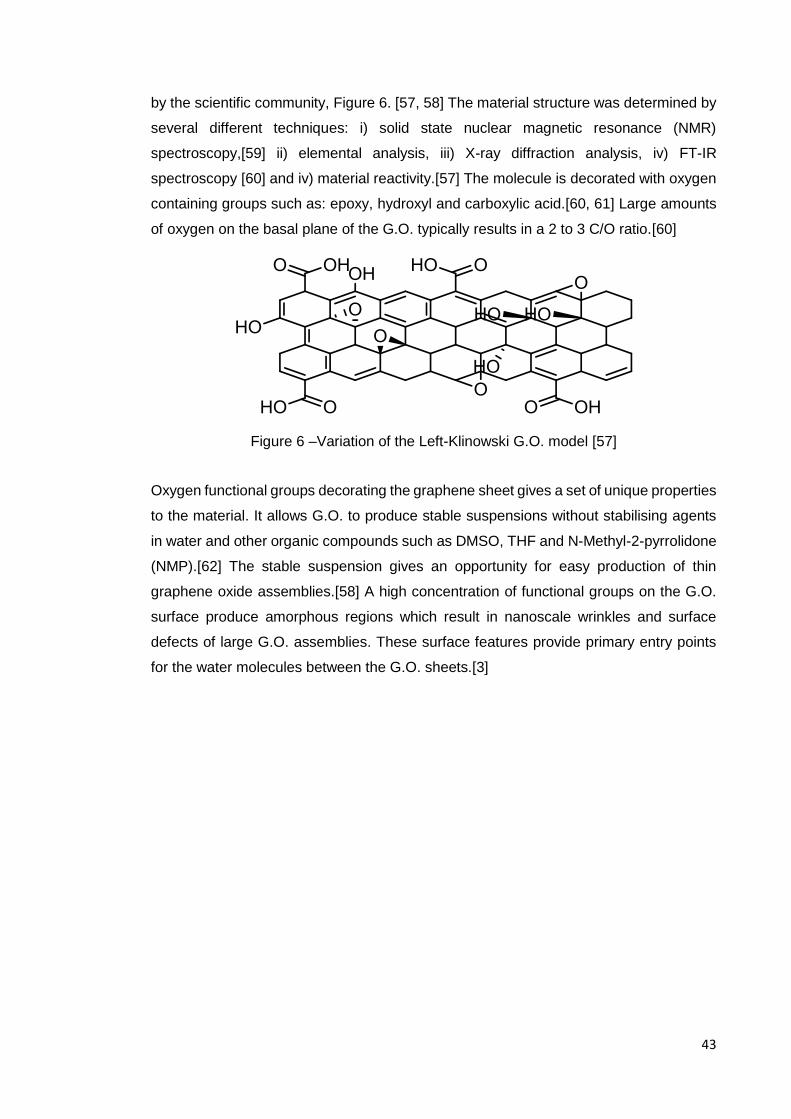
43

by the scientific community, Figure 6. [57, 58] The material structure was determined by

several different techniques: i) solid state nuclear magnetic resonance (NMR)

spectroscopy,[59] ii) elemental analysis, iii) X-ray diffraction analysis, iv) FT-IR

spectroscopy [60] and iv) material reactivity.[57] The molecule is decorated with oxygen

containing groups such as: epoxy, hydroxyl and carboxylic acid.[60, 61] Large amounts

of oxygen on the basal plane of the G.O. typically results in a 2 to 3 C/O ratio.[60]

Figure 6 –Variation of the Left-Klinowski G.O. model [57]

Oxygen functional groups decorating the graphene sheet gives a set of unique properties

to the material. It allows G.O. to produce stable suspensions without stabilising agents

in water and other organic compounds such as DMSO, THF and N-Methyl-2-pyrrolidone

(NMP).[62] The stable suspension gives an opportunity for easy production of thin

graphene oxide assemblies.[58] A high concentration of functional groups on the G.O.

surface produce amorphous regions which result in nanoscale wrinkles and surface

defects of large G.O. assemblies. These surface features provide primary entry points

for the water molecules between the G.O. sheets.[3]

44

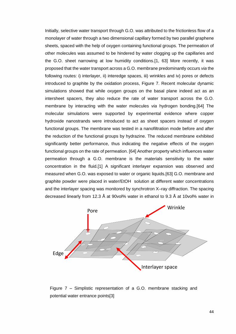
Initially, selective water transport through G.O. was attributed to the frictionless flow of a

monolayer of water through a two dimensional capillary formed by two parallel graphene

sheets, spaced with the help of oxygen containing functional groups. The permeation of

other molecules was assumed to be hindered by water clogging up the capillaries and

the G.O. sheet narrowing at low humidity conditions.[1, 63] More recently, it was

proposed that the water transport across a G.O. membrane predominantly occurs via the

following routes: i) interlayer, ii) interedge spaces, iii) wrinkles and iv) pores or defects

introduced to graphite by the oxidation process, Figure 7. Recent molecular dynamic

simulations showed that while oxygen groups on the basal plane indeed act as an

intersheet spacers, they also reduce the rate of water transport across the G.O.

membrane by interacting with the water molecules via hydrogen bonding.[64] The

molecular simulations were supported by experimental evidence where copper

hydroxide nanostrands were introduced to act as sheet spacers instead of oxygen

functional groups. The membrane was tested in a nanofiltration mode before and after

the reduction of the functional groups by hydrazine. The reduced membrane exhibited

significantly better performance, thus indicating the negative effects of the oxygen

functional groups on the rate of permeation. [64] Another property which influences water

permeation through a G.O. membrane is the materials sensitivity to the water

concentration in the fluid.[1] A significant interlayer expansion was observed and

measured when G.O. was exposed to water or organic liquids.[63] G.O. membrane and

graphite powder were placed in water/EtOH solution at different water concentrations

and the interlayer spacing was monitored by synchrotron X–ray diffraction. The spacing

decreased linearly from 12.3 Å at 90vol% water in ethanol to 9.3 Å at 10vol% water in

Wrinkle

Edge

Pore

Interlayer space

Figure 7 – Simplistic representation of a G.O. membrane stacking and

potential water entrance points[3]

45

ethanol. Interestingly, at 100vol% ethanol, the interlayer spacing increases to 10 Å. The

change in interlayer expansion/contraction was attributed to the varying number of water

monolayers intercalating G.O. material at different concentrations. This could explain the

varying rate of water permeation with respect to the relative humidity studied

previously.[1, 63]

To get a complete in depth model of water permeation through a G.O. membrane is very

challenging. The main issue stems from the aforementioned lack of understanding of the

exact G.O. chemical structure. Furthermore, a full permeation model should take into

account the physical microstructure of the material such as: sheet size, layer-by-layer

stacking, pores and wrinkles of the surface, which are difficult to define and vary among

membranes.[3]

1.4.1 Membrane manufacturing

An overview of the individual steps necessary for the production of G.O. membranes is

provided below and shown in the Figure 8. Typically, graphite powder is oxidised using

Hummer’s method [57], followed by exfoliation of the graphite powder using sonication

in deionised water. The suspension can then be coated on a wide range of ceramic or

polymeric supports by spray, spin, or filtration coating techniques.[1, 16, 58, 65] The

resulting film is water selective graphene oxide membrane.

Oxidation

Ultrasonication

Coating

H2O

Flexible Membrane

Spin

Spray

Filtration

Graphite Graphite Oxide

Suspended

Graphene

Oxide

Brodie’s Method

Hummer’s Method

Improved Hummer’s

Method

Figure 8 – Overview of the G.O. membrane production process

46

1.4.2 Brodie’s Method

The first graphene oxide was produced in 1859 by a British scientist while he was

investigating the structure of graphite. [66] One of the reactions involved adding “potash

chlorate”, potassium chlorate (KClO3), to a slurry of graphite and nitric acid. The success

of the oxidation was determined by measuring the product weight increase after the

reaction and separation. After 5 consecutive oxidation repeats the weight had stopped

increasing and the graphite was deemed to be fully oxidised. The graphite oxide was

able to disperse in deionised water and alkaline solutions, but did not dissolve in

acids.[66]

1.4.3 Hummers Method

In 1957, Brodie’s method was improved by S. Hummer and E. Offeman. The

concentrated nitric acid was replaced by sulphuric acid and the oxidising agent,

potassium chlorate, was replaced by potassium permanganate (KMnO4). [67] The exact

mechanism of the oxidation is still not clear, however it is postulated that the oxidative

species, dimanganese heptoxide 1, Scheme 1, intercalates between graphite plates and

oxidises the basal plane of the graphene.

Scheme 1-Dimanganese heptoxide formation[57]

Dimanganese heptoxide is a more reactive form of the potassium permanganate, which

is known to explode if heated above 55°C or in contact with organic materials. Therefore,

the process temperature has to be strictly monitored during the oxidation.[57, 67] The

resulting graphite oxide exfoliates in water very well with the help of a sonic bath.[1, 61]

1.4.4 Improved Hummers method

A recent explosion in graphite research has also led to improvements in G.O. synthesis.

Improved methods are based on the previously described Hummer’s method.[68, 69]

The main improvement involves excluding sodium nitrate (NaNO3) [69] and introducing

phosphoric acid into the mixture.[68] The exclusion of NaNO3 eliminated the production

of toxic gases without loss of the oxidation in terms of functionality and overall yield.[69]

47

1.4.5 Coating

The coating procedure is a crucial part of the membrane manufacturing process. Initial

G.O. membrane research conducted at the University of Manchester used spin and

spray coating techniques on a heated 25 µm copper foil to produce a uniform G.O.

membrane layer. Later, the copper foil was chemically etched away to expose a free

standing G.O. layer for experimentation.[1]

By far the most common coating procedure is vacuum filtration, with this technique being

used by a large number of researchers for G.O. membrane preparation Figure 9.[16] The

method involves a three-piece vacuum filter. The G.O. suspension is loaded in the top

part of the apparatus and is allowed to pass through a support. The filtration differential

pressure is usually kept at approximately 1 atm.

G.O. solution in a container

G.O. membrane Perforated

metal or plastic disc

Water

Vacuum

Figure 9 – Typical three piece vacuum filter

48

1.5 G.O. Membranes Selective Water Separations

The first recorded graphite oxide use as a water selective membrane was published in a

patent in 1969. The graphite oxide was prepared using Hummers method, but not

exfoliated by sonication. Instead graphite oxide was used it its particle form to produce

a thin film on cellulose paper. The thin graphite oxide layer was then coated with a

cyanoethylated polyvinyl alcohol polymer and post process baking at 150°C for 30 min.

The resulting 5 µm membrane was tested in a reverse osmosis laboratory apparatus at

≈ 69bar trans- membrane pressure using 3.5wt% NaCl solution. The membrane

selectivity was low with 72% of salt going through the membrane. After 24h operation a

sample was taken and an average pervaporation flux was estimated as 1.1 L h-1m-2.[70]

1.5.1 Polymer supported and free standing G.O. membranes

In 2012, Nair et al. exfoliated graphite oxide in water and produced graphene oxide

suspension. The suspension was then used to produce a graphite oxide thin film on a

copper metal surface. The copper was chemically etched away, which exposed a

freestanding membrane. The membrane was used in vapour permeation tests of various

liquids and gases at a room temperature.

Initial tests were conducted on a submicrometer thick G.O. membrane at room

temperature using helium and hydrogen gas. The experimental setup is shown in Figure

10 a). Helium permeation was studied using a mass spectrometer. The permeation

experiments showed no detectable loss of helium, thus the rate of permeation was

assumed to be lower than the accuracy of the mass-spectrometer, which resulted in an

estimated rate of permeation of 3.6*10-8 kg h-1m-2bar-1. A 12 µm thick polyethylene

terephthalate film was used as a reference barrier. The leakage rate resulted in 3*10-5

kg h-1m-2bar-1 the rate of permeation, which was ≈ 833.3 times higher. Similar results

were found using hydrogen gas with no meaningful rate of permeation measured;

although it has to be noted that the accuracy of detection was three orders of magnitude

lower.[1]

49

To test liquid vapour rate of permeation the experimental setup was changed, Figure 10

b). The vapour permeation was measured by recording the weight loss of the vessel

placed on a computerised balance. A vessel covered with a 1 µm thick G.O. film did not

show any weight loss after several days for hexane, acetone, decane, propanol and

interestingly ethanol; with a detection limit of 1 mg. However, a large weight loss was

observed when the container was filled with water. The rate of water loss through the

G.O. membrane was the same as the weight loss without a membrane, under the same

experimental conditions. A summary of the liquid and gas fluid rates of permeation is

shown in Table 4.[1]

Liquid Mixture

Computerised Balance

Glove Box

b)

He/H2

Leak Detector

Pump

a)

Figure 10 – Permeation experiments a) gas experiment setup b) water

experiment setup[1]

50

Table 4-Summary of fluid permeation experiments at room temperature [1]

Membrane Fluid Rate of permeation

<1 µm Helium 3.6*10-8 kg h-1m-2bar-1

<1 µm Hydrogen 3.6*10-5 kg h-1m-2bar-1

1 µm Water 0.48 kg h-1m-2

Open apparatus Water 0.54 kg h-1m-2

1 µm Hexane N/A

1 µm EtOH N/A

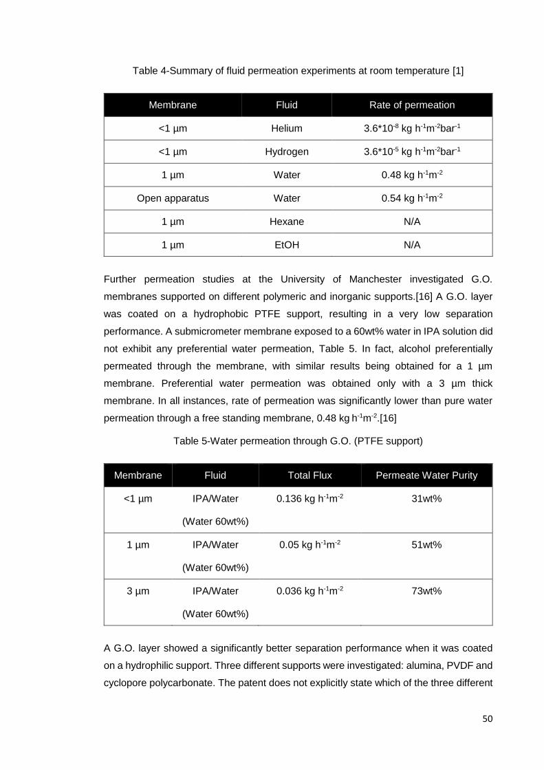
Further permeation studies at the University of Manchester investigated G.O.

membranes supported on different polymeric and inorganic supports.[16] A G.O. layer

was coated on a hydrophobic PTFE support, resulting in a very low separation

performance. A submicrometer membrane exposed to a 60wt% water in IPA solution did

not exhibit any preferential water permeation, Table 5. In fact, alcohol preferentially

permeated through the membrane, with similar results being obtained for a 1 µm

membrane. Preferential water permeation was obtained only with a 3 µm thick

membrane. In all instances, rate of permeation was significantly lower than pure water

permeation through a free standing membrane, 0.48 kg h-1m-2.[16]

Table 5-Water permeation through G.O. (PTFE support)

Membrane Fluid Total Flux Permeate Water Purity

<1 µm IPA/Water

(Water 60wt%)

0.136 kg h-1m-2 31wt%

1 µm IPA/Water

(Water 60wt%)

0.05 kg h-1m-2 51wt%

3 µm IPA/Water

(Water 60wt%)

0.036 kg h-1m-2 73wt%

A G.O. layer showed a significantly better separation performance when it was coated

on a hydrophilic support. Three different supports were investigated: alumina, PVDF and

cyclopore polycarbonate. The patent does not explicitly state which of the three different

51

materials were used as a support for the tabulated pervaporation results, Table 6. The

selectivity of the membranes was significantly better and water enrichment in the

permeate was obtained with micrometre thick membranes.[16]

Table 6-Water permeation through G.O. (hydrophilic support) [16]


<1 µm IPA/Water

(Water 60wt%)

0.042 kg h-1m-2 52wt%

1 µm IPA/Water

(Water 60wt%)

0.038 kg h-1m-2 78wt%

5 µm IPA/Water

(Water 60wt%)

0.027 kg h-1m-2 66wt%

52

It is important to note that all experiments were conducted at room temperature in a

vapour permeation mode. The membrane testing apparatus limited the ability to examine

a wider scope of temperatures. Furthermore, no agitation was present at the surface of

the membrane, which is known to negatively influence the rate of permeation and

membrane selectivity.[11]

T. Yeh et al. investigated a multi-layered G.O. membrane performance in a pervaporation

mode; liquid in contact with a membrane. Membranes were tested using permeation cell

manufactured by Sulzer Chemtech.[71, 72]

The G.O. layer was coated on a thin film nanofibrous composite support. The support

was composed of the following three parts:

1. Cellulose-an ultrafine nanofibrous top layer (in direct contact with G.O.)

2. Polyacrylonitrile-an electro spun nanofibrous middle layer

3. Polyethylene terephthalate-nonwoven microfibrous support

An ultrafine cellulose was able to hold a flaw-free G.O. layer over a wide range of

thicknesses, 97-618 nm. As a model test solution, 20wt% water in EtOH at 70°C was

selected for the study. The highest permeation flux of water, 2.2 kg h-1m-2, was obtained

using 97nm G.O. layer. The permeate purity was slightly lower, 98.7wt%, when

compared to the thicker, ≈ 620 nm, membrane which resulted in a 99.0wt% permeate

purity. The higher permeate quality produced by a thicker membrane came at the

expense of a significantly lower rate of permeation,0.9 kg h-1m-2, Table 7 Entry 1 and

2.[71]

Liu R et al. studied selective water permeation using a number of different aqueous

alcohol mixtures.[73] The G.O. was coated on a PTFE polymeric support and the

selective fluid separation was tested by placing the membrane into a three-piece filter.

The bottom part of the filter was connected to a vacuum pump while the top part was

loaded with the liquid of interest at room temperature.[73] In all instances, 5 µm thick

membranes were used. It is important to note that the permeation fluxes were expressed

as a function of water vapour pressure and a membrane thickness in the original

publication.[73] The results shown in the Table 7 Entry 3 and 4 were converted to a form

comparable with the results in the previous and the remainder of the document.

The permeation rate measured was considerably higher than that reported in the

previous research at room temperature with higher water content and thinner or

comparable thickness membranes Table 5 and Table 6. The selectivity of the

membranes was also better than the membranes tested at the University of

Manchester.[16] The separation magnitude and the permeation fluxes were closer to the

53

G.O. membranes tested in a pervaporation cell at higher temperatures Table 7 Entry 1

and 2.

Table 7-Organic compound dehydration using G.O. membrane.

Entry Membrane Fluid Total Flux Permeate Water

Purity

Reference

1 0.093 µm EtOH/Water

(Water 20wt%)

2.2 kg h-1m-2 98.4wt% [71]

2 0.62 µm EtOH/Water

(Water 20wt%)

0.9 kg h-1m-2 99wt% [71]

3 5 µm EtOH/Water

(Water 25wt%)

1.23 kg h-1m-2 ≈ 80wt% [73]

4 5 µm IPA/Water

(Water 25wt%)

1.44 kg h-1m-2 ≈ 90wt% [73]

Tang. Y. P. et al. studied membrane fabrication pressure influence on separation

performance. All membranes were assembled and tested in a dead end pressurised

system.[74] The pervaporation rig was set up to provide rapid agitation above the

membrane surface, which allowed minimisation of the concentration polarization, which

may have been present in the previous pervaporation tests. All tests were performed at

room temperature using mainly 2 µm thick G.O. selective layer. Aqueous ethanol solution

was selected as a test fluid.[17]

It was found that membrane permeation flux and selectivity were sensitive to the

membrane assembly pressure, Table 8. The highest permeate purity, 98wt%, water, was

recorded for a membrane assembled under 5 bar pressure. However, the same

membrane also exhibited the lowest permeation flux, 0.26 kg h-1m-2. Interestingly, a much

higher permeation flux, 0.34 kg h-1m-2, was measured using a membrane assembled

under 20 bar pressure. This came at the cost of a significantly reduced permeate quality,

which dropped to 89.8wt%. It was postulated that the highest membrane coating

pressure produced rapid G.O. deposition leading to multiple surface flaws, thus resulting

in a lower permeate purity.[17]

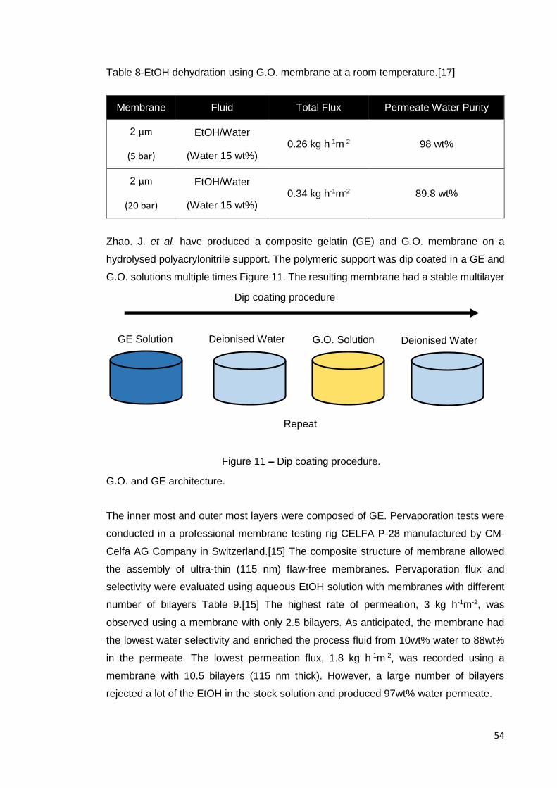
54

Table 8-EtOH dehydration using G.O. membrane at a room temperature.[17]


2 µm

(5 bar)

EtOH/Water

(Water 15 wt%) 0.26 kg h-1m-2 98 wt%

2 µm

(20 bar)

EtOH/Water

(Water 15 wt%) 0.34 kg h-1m-2 89.8 wt%

Zhao. J. et al. have produced a composite gelatin (GE) and G.O. membrane on a

hydrolysed polyacrylonitrile support. The polymeric support was dip coated in a GE and

G.O. solutions multiple times Figure 11. The resulting membrane had a stable multilayer

G.O. and GE architecture.

The inner most and outer most layers were composed of GE. Pervaporation tests were

conducted in a professional membrane testing rig CELFA P-28 manufactured by CM-

Celfa AG Company in Switzerland.[15] The composite structure of membrane allowed

the assembly of ultra-thin (115 nm) flaw-free membranes. Pervaporation flux and

selectivity were evaluated using aqueous EtOH solution with membranes with different

number of bilayers Table 9.[15] The highest rate of permeation, 3 kg h-1m-2, was

observed using a membrane with only 2.5 bilayers. As anticipated, the membrane had

the lowest water selectivity and enriched the process fluid from 10wt% water to 88wt%

in the permeate. The lowest permeation flux, 1.8 kg h-1m-2, was recorded using a

membrane with 10.5 bilayers (115 nm thick). However, a large number of bilayers

rejected a lot of the EtOH in the stock solution and produced 97wt% water permeate.

Dip coating procedure

GE Solution Deionised Water G.O. Solution Deionised Water

Repeat

Figure 11 – Dip coating procedure.

55

Table 9-EtOH dehydration using G.O. membrane at 77°C.[15]


2.5

(bilayers)

EtOH/Water

(Water 10 wt%)

3 kg h-1m-2 88 wt%

4.5

(bilayers)

EtOH/Water

(Water 10 wt%)

2.4 kg h-1m-2 92 wt%

6.5

(bilayers)

EtOH/Water

(Water 10 wt%)

2.2 kg h-1m-2 93 wt%

8.5

(bilayers)

EtOH/Water

(Water 10 wt%)

2 kg h-1m-2 95 wt%

10.5

(bilayers)

EtOH/Water

(Water 10 wt%)

1.8 kg h-1m-2 97 wt%

1.5.2 Ceramic Supported Graphene Oxide

Huang. K. et al. have coated a ceramic hollow fibre membrane with G.O. by vacuum

suction. The ceramic tube coated with G.O. was tested by submerging it into a vessel

filled with 97.4-99wt% dimethyl carbonate (DMC) and water solution at 25-40°C. Several

selected results are shown in Table 10. An extraordinary fast water permeation, 1.1 kg

h-1m-2, was observed at only 2wt% in DMC at 25°C. To the best of our knowledge, this is

the best-recorded rate of permeation for a room temperature operation at 2wt%.

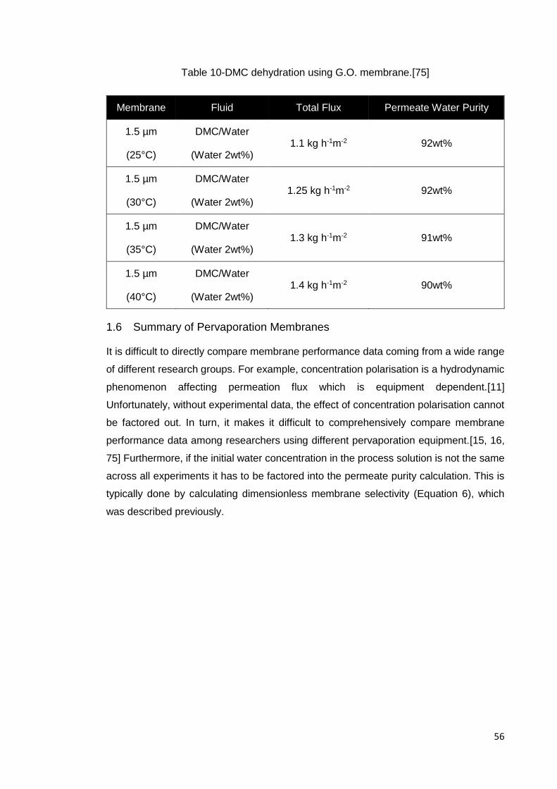
56

Table 10-DMC dehydration using G.O. membrane.[75]


1.5 µm

(25°C)

DMC/Water

(Water 2wt%) 1.1 kg h-1m-2 92wt%

1.5 µm

(30°C)

DMC/Water

(Water 2wt%) 1.25 kg h-1m-2 92wt%

1.5 µm

(35°C)

DMC/Water


1.5 µm

(40°C)

DMC/Water


1.6 Summary of Pervaporation Membranes

It is difficult to directly compare membrane performance data coming from a wide range

of different research groups. For example, concentration polarisation is a hydrodynamic

phenomenon affecting permeation flux which is equipment dependent.[11]

Unfortunately, without experimental data, the effect of concentration polarisation cannot

be factored out. In turn, it makes it difficult to comprehensively compare membrane

performance data among researchers using different pervaporation equipment.[15, 16,

75] Furthermore, if the initial water concentration in the process solution is not the same

across all experiments it has to be factored into the permeate purity calculation. This is

typically done by calculating dimensionless membrane selectivity (Equation 6), which

was described previously.

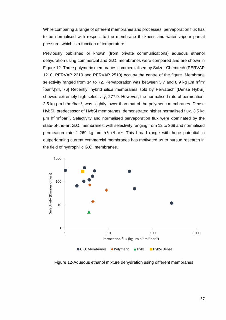
57

While comparing a range of different membranes and processes, pervaporation flux has

to be normalised with respect to the membrane thickness and water vapour partial

pressure, which is a function of temperature.

Previously published or known (from private communications) aqueous ethanol

dehydration using commercial and G.O. membranes were compared and are shown in

Figure 12. Three polymeric membranes commercialised by Sulzer Chemtech (PERVAP

1210, PERVAP 2210 and PERVAP 2510) occupy the centre of the figure. Membrane

selectivity ranged from 14 to 72. Pervaporation was between 3.7 and 8.9 kg µm h-1m-

2bar-1.[34, 76] Recently, hybrid silica membranes sold by Pervatech (Dense HybSi)

showed extremely high selectivity, 277.9. However, the normalised rate of permeation,

2.5 kg µm h-1m-2bar-1, was slightly lower than that of the polymeric membranes. Dense

HybSi, predecessor of HybSi membranes, demonstrated higher normalised flux, 3.5 kg

µm h-1m-2bar-1. Selectivity and normalised pervaporation flux were dominated by the

state-of-the-art G.O. membranes, with selectivity ranging from 12 to 369 and normalised

permeation rate 1-269 kg µm h-1m-2bar-1. This broad range with huge potential in

outperforming current commercial membranes has motivated us to pursue research in

the field of hydrophilic G.O. membranes.

Figure 12-Aqueous ethanol mixture dehydration using different membranes

1

10

100

1000

1 10 100 1000

Sele

ctiv

ity

(Dim

nes

ion

less

)

Permeation flux (kg µm h-1 m-2 bar-1)

G.O. Membranes Polymeric Hybsi HybSi Dense

58

2 Pervaporation Modelling

To understand and predict pervaporation technology feasibility on a large scale it is

essential to be able to model the process computationally. To do so, it is crucial to

understand principles of water transport through dense membranes. This chapter will

focus on the pervaporation mathematical modelling a process analysis. Predominantly,

two different models have been applied for pervaporation modelling i) the pore-flow

model, and ii) the solution-diffusion model. The pore-flow model is discussed briefly in

this chapter by proving the main concept of the model and the governing equations. The

solution-diffusion model is analysed in detail and is used in the further chapters for the

pervaporation through G.O. membranes modelling. The model was also used to create

a pervaporation simulation tool, which estimates the required membrane area for a

desired water/organic compound separation problem.

59

2.1 Pore-flow model

One of the main models, pore-flow model, is based on the following assumptions: i) part

of the pore is initially filled with liquid where liquid phase diffusion takes place, ii) liquid

changes into vapour inside the pore, iii) the permeant is transported through the vapour

filled portion of the pore to the permeate side.[77]

The main difference between the pore-flow model and the solution-diffusion model is the

pressure gradient inside the membrane Figure 13 a). In the pore-flow model, the

pressure drop (P) across the membrane produces a change in the chemical potential

(µ), which results in the separation driving force. The solvent activity (ɣiCw) remains

unchanged throughout the membrane. In the solution–diffusion model, the pressure

remains the same in the membrane and the concentration change produces a chemical

potential gradient.

The pore-flow model assumes that there is a number of straight cylinder shaped pores

of a length y penetrating the selective membrane layer from the process to the permeate

side at isothermal conditions.[77] Figure 13 b) shows a schematic representation of the

pore-flow model. The pore is partially filled with the permeating liquid without any

separation. The distance of the penetration is denoted as a ya. In the liquid filled section

the permeant flows by liquid phase transport. The liquid section is followed by a vapour

section with a length yb. In this section, the permeant flows by vapour phase transport.

The evaporation of the permeant takes place at the interface of a liquid-vapour boundary

in the pore of the membrane. These assumptions allow pervaporation to be modelled as

a combination of the liquid phase and vapour phase transport in series. [78]

60

Figure 13-Pore-flow model a) depiction of the core concepts, b) schematic

representation of the model.[2, 77]

𝑦𝑚

Membrane

P*

𝑦𝑎 yb

Permeate (vapour) Process fluid (liquid)

P1

xw,1

yw,*

P2

xw,*

yw,2

Chemical potential, µi

Pressure, P

Solvent activity, γiC

i

High pressure

solution

Membrane Low pressure

vapour

a)

b)

61

The mass transport of a single component in the liquid phase is described by Darcy’s

Law shown in Equation 5 and Equation 6.

𝑄𝑙𝑖𝑞𝑢𝑖𝑑 =𝑋

𝑦𝑎(𝑃1 − 𝑃∗)

Equation 5

𝑋 =𝜋𝑟4𝜌𝑁𝑡

8𝜂𝐿𝑀𝑖

Equation 6

Where, Qliquid is molar liquid flux (mol m-2s-1), X is combined pore-flow model coefficient

(mol bar-1s-1 m-1), r is the mean pore diameter (m),ρ is the fluid density (kg m-3),Nt is the

total number of pores per effective membrane area (m-2),ηL is viscosity of the fluid (kg m-

1 s-1), and Mi the molecular weight of the component (kg mol-1). The driving force in the

liquid filled region is expressed as a pressure difference between the liquid, P1 (bar), and

saturated vapour pressure in the pore, P* (bar).

For the vapour transport in the pore, several other assumptions are made. The pore is

assumed to be so small that vapour adsorbed onto the surface of the pore occupies

almost the entire space. This assumption means that all vapour transport is conducted

via the surface flow mechanism, a gas flow model originally defined and applied by

Gilliland.[77, 79]

This assumption of the vapour flow sets an upper pore size limit, 1-10-1-9 m, where this

model is valid. If the pore is large enough to accommodate Knudsen flow the model

becomes inapplicable. Also, the validity of Henry’s law is assumed. Based on the

assumptions of the vapour phase transport the molar flux can be calculated using

Equation 7 and Equation 8.

𝑄𝑉𝑎𝑝𝑜𝑢𝑟 = 𝑄𝑆𝑢𝑟𝑓𝑎𝑐𝑒 =𝑍

𝑦𝑏

((𝑃∗)2 − (𝑃2)2) Equation 7

𝑍 =𝜋(2𝑟𝑡𝑎 − 𝑡𝑎

2)2𝑡𝑎𝑁𝑡

8𝑟

𝑅𝑇

𝜂𝐺

(𝑘𝐻′ )2

Equation 8

Where, QVapour is vapour molar flux (mol m-2s-1),ta Is the thickness of the adsorbed

monolayer of the gas (m),R is the ideal gas constant (m3 bar K-1mol-1),T is temperature

(K),ηG is viscosity (kg m-1 s-1), and k’H is the product of the weight of the

membrane/volume of adsorbed gas molecules and Henry’s constant (mol m-3bar-1). The

vapour phase driving force is a square pressure difference between saturated vapour

pressure and the permeate pressure respectively.

The combination of the liquid flow, Equation 5, and vapour flow, Equation 7, leads to the

total molar flux expression Equation 9

62

𝑄𝑡𝑜𝑡𝑎𝑙 =𝑋

𝑦(𝑃1 − 𝑃∗) +

𝑍

𝑦((𝑃∗)2 − (𝑃2)2)

Equation 9

There are several variations of the Equation 9 that are important to note. Equation 9 is

valid only when P2 < P*. If the pressure of the permeate side is greater than the saturated

liquid vapour pressure,P2 ≥ P* the entire pore fills up with a liquid permeate. In this

instance the permeation equation can be reduced to the liquid phase transport resistance

(Equation 10).

𝑄𝑡𝑜𝑡𝑎𝑙 =𝑋

𝑦𝑎(𝑃1 − 𝑃2)

Equation 10

For a binary mixture the equation has to be changed to include individual rates of

permeation. A binary pair liquid phase, for instance water and organic component,

transport rate remains the same (Equation 11).

𝑄𝑙𝑖𝑞𝑢𝑖𝑑 =𝑍𝑚𝑖𝑥𝑡𝑢𝑟𝑒

𝑦𝑎(𝑃1 − 𝑃∗)

Equation 11

However the rate of vapour transport model has to be changed to reflect different rates

of permeation of each component, Equation 12 and Equation 13.

𝑄𝑤,𝑉𝑎𝑝𝑜𝑢𝑟 =𝑍𝑤

𝑦𝑏

((𝑃𝑤∗)2 − (𝑃𝑤,2)

2)

Equation 12

𝑄𝑜𝑟𝑔,𝑉𝑎𝑝𝑜𝑢𝑟 =𝑍𝑜𝑟𝑔

𝑦𝑏((𝑃𝑂𝑟𝑔

∗ )2

− (𝑃𝑂𝑟𝑔,2)2

) Equation 13

A total molar permeate flux is then expressed by a combination of the Equation 11,

Equation 12 and Equation 13, which yields Equation 14.

𝑄𝑇𝑜𝑡𝑎𝑙 =𝑋𝑚𝑖𝑥𝑡𝑢𝑟𝑒

𝑦𝑎

(𝑃1 − 𝑃∗) +𝑍𝑤

𝑦𝑏((𝑃𝑊

∗ )2 − (𝑃𝑊,2)2

) +𝑍𝑜𝑟𝑔

𝑦𝑏((𝑃𝑂𝑟𝑔

∗ )2

− (𝑃𝑂𝑟𝑔,2)2

)

Equation 14

According to the pore-flow model, the membrane separation power stems from the

different rates of adsorbed layer permeation. The permeate purity, vapour mole fraction,

can be calculated by estimating the rate of permeation ratio (Equation 15). The

expression requires partial vapour pressure of both components, which are usually

known for a typical binary system. To calculate individual component enrichment in the

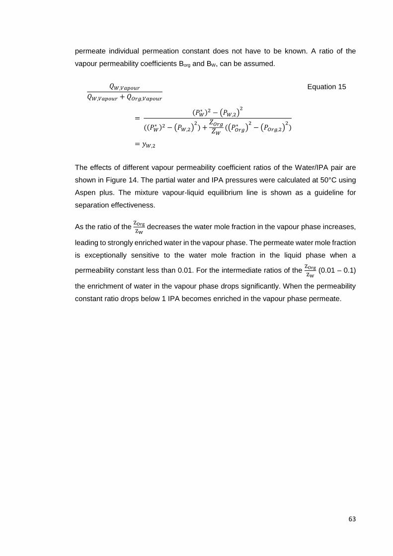
63

permeate individual permeation constant does not have to be known. A ratio of the

vapour permeability coefficients Borg and BW, can be assumed.

𝑄𝑊,𝑉𝑎𝑝𝑜𝑢𝑟

𝑄𝑊,𝑉𝑎𝑝𝑜𝑢𝑟 + 𝑄𝑂𝑟𝑔,𝑉𝑎𝑝𝑜𝑢𝑟

= (𝑃𝑊

∗ )2 − (𝑃𝑊,2)2

((𝑃𝑊∗ )2 − (𝑃𝑊,2)

2) +

𝑍𝑂𝑟𝑔

𝑍𝑊((𝑃𝑂𝑟𝑔

∗ )2

− (𝑃𝑂𝑟𝑔,2)2

)

= 𝑦𝑊,2

Equation 15

The effects of different vapour permeability coefficient ratios of the Water/IPA pair are

shown in Figure 14. The partial water and IPA pressures were calculated at 50°C using

Aspen plus. The mixture vapour-liquid equilibrium line is shown as a guideline for

separation effectiveness.

As the ratio of the ZOrg

ZW decreases the water mole fraction in the vapour phase increases,

leading to strongly enriched water in the vapour phase. The permeate water mole fraction

is exceptionally sensitive to the water mole fraction in the liquid phase when a

permeability constant less than 0.01. For the intermediate ratios of the ZOrg

ZW (0.01 – 0.1)

the enrichment of water in the vapour phase drops significantly. When the permeability

constant ratio drops below 1 IPA becomes enriched in the vapour phase permeate.

64

Figure 14 – Pore-flow model predictions of permeate water mole fraction[77]

The pore-flow model is valid for membranes with small pores in the range of 1-10 – 1.5-9

m.[77] G.O. falls in this range by having an approximate pore size of 3.49-10 m and an

intersheet spacing of 6.89-10 m, thus pore-flow model should be applicable.[80] For a

more detailed pore-flow model derivation the reader is referred to the original

publication.[81]

2.2 Solution-diffusion model

Currently, solution-diffusion is the main model used to explain the pervaporation

process.[18] The model is based on the assumption that the permeating species

dissolves in the membrane material and then diffuses through the thickness of the

membrane.[2] The rate of permeation is based on the concentration gradient, which is

mathematically related to the chemical potential. The selectivity of a membrane is the

result of different partitioning coefficients of the compounds into the membrane matrix. A

simplified image of the main concepts behind the solution-diffusion model are shown in

Figure 15. The solution-diffusion model assumes that a pressure applied across a dense

membrane is distributed everywhere evenly and is constant across the thickness of the

membrane. In this model, the driving force is expressed as a concentration gradient

within the membrane, which is linked to the chemical potential and in turn can be

mathematically expressed as a partial pressure of the permeating component. [2]

0

0.1

0.2

0.3

0.4

0.5

0.6

0.7

0.8

0.9

1

0 0.1 0.2 0.3 0.4 0.5 0.6 0.7 0.8 0.9 1

Wat

er

per

mea

te m

old

e fr

acti

on

, yw

ater

Water mole fraction in the process liquid, xwater

Ratio = 0.1 Ratio = 1 VLERatio = 0.01 Ratio = 0.001 Ratio = 1045°

65

The mass flux through a dense membrane is expressed by Fick’s law, Equation 16:

𝐽 = −𝐷𝑤

𝑑𝜌𝑤

𝑑𝑦𝑚

Equation 16

Where, J is the mass flux of the permeating species (kg m-2s-1), Dw is the diffusion

coefficient (m2s-1), and δm is the thickness of the membrane (m).

𝜌𝑤 = 𝐶𝑤𝑀𝑤𝑥𝑤 Equation 17

The ρw is mass concentration (kg m-3),Cw is molar concentration (mol m-3),Mw is the

molecular weight (g mol-1), and xw is the mole fraction (mol mol-1).

Upon integration over the thickness of the membrane Equation 16 leads to Equation 18.

𝐽 =𝐷𝑤(𝜌𝑤,𝑀𝐿 − 𝜌𝑤,𝑀𝑆)

𝑦𝑚

Equation 18

The Equation 18 is a fundamental expression relating mass concentration on the process

side next to the membrane surface (ρw,ML) and the permeate leaving the membrane and

entering the support layer (ρw,MS) to the pervaporation flux (J) with respect to the

membrane thickness (ym).

The general expression, Equation 18, is derived from the chemical potential differential

Equation 19. The expression links the change of the chemical potential to the mole

fraction and pressure changes.

Chemical potential, µi

Pressure, P

Solvent activity, γiC

i

High pressure

solution

Membrane Low pressure

vapour

Figure 15 – Schematics of the solution diffusion concepts[2]

𝑦𝑙 𝑦𝑚 𝑦

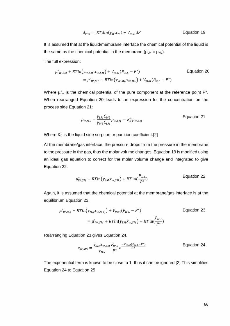
66

𝑑𝜇𝑊 = 𝑅𝑇𝑑𝑙𝑛(𝛾𝑊𝑥𝑊) + 𝑉𝑚𝑜𝑙𝑑𝑃 Equation 19

It is assumed that at the liquid/membrane interface the chemical potential of the liquid is

the same as the chemical potential in the membrane (µLM = µML).

The full expression:

𝜇˚𝑊,𝐿𝑀 + 𝑅𝑇𝑙𝑛(𝛾𝑤,𝐿𝑀 𝑥𝑤,𝐿𝑀) + 𝑉𝑚𝑜𝑙(𝑃𝑤.𝐿 − 𝑃∗)

= 𝜇˚𝑊,𝑀𝐿 + 𝑅𝑇𝑙𝑛(𝛾𝑊,𝑀𝐿𝑥𝑤,𝑀𝐿) + 𝑉𝑚𝑜𝑙(𝑃𝑤.𝐿 − 𝑃∗)

Equation 20

Where µ°w is the chemical potential of the pure component at the reference point P*.

When rearranged Equation 20 leads to an expression for the concentration on the

process side Equation 21:

𝜌𝑤,𝑀𝐿 =𝛾𝐿𝑀𝐶𝑀𝐿

𝛾𝑀𝐿𝐶𝐿𝑀𝜌𝑤,𝐿𝑀 = 𝐾𝑆

𝐿𝜌𝑤,𝐿𝑀 Equation 21

Where KSL is the liquid side sorption or partition coefficient.[2]

At the membrane/gas interface, the pressure drops from the pressure in the membrane

to the pressure in the gas, thus the molar volume changes. Equation 19 is modified using

an ideal gas equation to correct for the molar volume change and integrated to give

Equation 22.

𝜇𝑊.𝑆𝑀∘ + 𝑅𝑇𝑙𝑛(𝛾𝑆𝑀𝑥𝑤,𝑆𝑀) + 𝑅𝑇 ln (

𝑃𝑤.𝐿

𝑃∗)

Equation 22

Again, it is assumed that the chemical potential at the membrane/gas interface is at the

equilibrium Equation 23.

𝜇˚𝑊,𝑀𝑆 + 𝑅𝑇𝑙𝑛(𝛾𝑀𝑆𝑥𝑤,𝑀𝑆)) + 𝑉𝑚𝑜𝑙(𝑃𝑤.𝐿 − 𝑃∗)

= 𝜇˚𝑊,𝑆𝑀 + 𝑅𝑇𝑙𝑛(𝛾𝑆𝑀𝑥𝑤,𝑆𝑀) + 𝑅𝑇 ln(𝑃𝑤.𝐿

𝑃∗)

Equation 23

Rearranging Equation 23 gives Equation 24.

𝑥𝑤,𝑀𝑆 =𝛾𝑆𝑀𝑥𝑤,𝑆𝑀

𝛾𝑀𝑆

𝑃𝑤.𝐿

𝑃∗𝑒

−𝑉𝑚𝑜𝑙(𝑃𝑤.𝐿−𝑃∗)𝑅𝑇

Equation 24

The exponential term is known to be close to 1, thus it can be ignored.[2] This simplifies

Equation 24 to Equation 25

67

𝑥𝑤,𝑀𝑆 =𝛾𝑆𝑀𝑥𝑤,𝑆𝑀

𝛾𝑀𝑆

𝑃𝑤.𝐿

𝑃∗

Equation 25

The product of the xw,γSM Pw.L can be replaced by a partial pressure term on the permeate

side Pp and simplified to Equation 26

𝜌𝑤,𝑀𝑆 = 𝑀𝑤𝐶𝑤,𝑀𝑆

𝛾𝑆𝑀

𝛾𝑀𝑆𝑃∗𝑃𝑤.𝑝 = 𝐾𝑆

𝐺𝑃𝑤.𝑝 Equation 26

Where KSG = Mw CwMS γSM γ-1

MS P*-1 is the gas phase sorption coefficient.

The concentration change across the membrane is now fully defined. The driving force

gradient in Fick’s law, Equation 18, can now be replaced to derive the membrane flux

Equation 27.

𝐽 =𝐷𝑤(𝐾𝑆

𝐿𝜌𝑤,𝐿𝑀 − 𝐾𝑆𝐺𝑃𝑤.𝑝)

𝑦𝑚

Equation 27

However, Equation 21 contains the liquid sorption coefficient while Equation 26 has gas

sorption coefficient. The interconversion of these coefficients is handled by considering

a hypothetical vapour-liquid equilibrium Equation 28. [82]

𝜇𝑊∘ + 𝑅𝑇𝑙𝑛(𝛾𝐿𝑥𝑤

𝐿 ) + 𝑉𝑚𝑜𝑙(𝑃𝑤.𝐿 − 𝑃∗)

= 𝜇𝑊∘ + 𝑅𝑇𝑙𝑛(𝛾𝐺𝑥𝑤

𝐺 ) + 𝑅𝑇 ln(𝑃𝑤.𝐿

𝑃∗)

Equation 28

Using the same rearrangement as in Equation 23, Equation 24, Equation 25 and

Equation 26 the vapour liquid equilibrium become Equation 29.

𝜌𝑤𝐿 = 𝑀𝑤𝐶𝑤

𝛾𝐺

𝛾𝐿𝑃∗𝑃𝑤.𝐿 =

𝐾𝑆𝐺

𝐾𝑆𝐿 𝑃 𝑤.𝐿

Equation 29

Where PW.L is the partial vapour pressure of water in equilibrium with the feed liquid. It is

worth noting that the term Mw Cw γG γ-1(L) P-1(*) is also known as Henry’s law coefficient,

H.

Combining, Fick’s law, Equation 27 and Equation 29, results in a pressure normalised

pervaporation flux Equation 30.

68

𝐽 =𝐷𝑤𝐾𝑆

𝐺(𝑃 𝑤.𝐿 − 𝑃𝑃)

𝑦𝑚= 𝑘𝑀.𝑃(𝑃 𝑤.𝐿 − 𝑃𝑤.𝑃)

Equation 30

Where kM.P (g m-2bar-1s-1) is a pressure normalised pervaporation coefficient. By selecting

a partial vapour pressure as a driving force, the normalized permeability coefficient

becomes kM.P = kL.P.GO/ym, where kL.P.GO is the permeability constant (g m bar-1m-2s-1) and

δm is membrane thickness (m). The change in the feed composition and the temperature

is reflected by the change in partial vapour pressure.[71, 83]

The process liquid was considered as non-ideal solution. The vapour pressure was

calculated using Equation 31. The water activity coefficient was calculated using Aspen

Plus software.

𝑃𝑤.𝐿 = 𝑃𝑤∗𝑥𝑤 𝛾𝑤 Equation 31

The saturated vapour pressure of pure component was calculated using the Antoine

Equation 32

log10 𝑃∗ = A𝑎𝑛𝑡𝑜𝑖𝑛𝑒 − 𝐵𝑎𝑛𝑡𝑜𝑖𝑛𝑒

𝐶𝑎𝑛𝑡𝑜𝑖𝑛𝑒 + 𝑇

Equation 32

Where A, B and C are material constants (Table 11) and T (K) is temperature.

Table 11-Antoine constants for water in the temperature range 273-303 K [84]

Parameter Value

Aantoine (bar) 5.40

Bantoine (bar K-1) 1838.68

Cantoine (K) -31.74

2.3 Concentration polarisation

The main membrane performance criteria are permeation flux and selectivity. A rate of

the permeating species through a membrane is affected by a number of different

parameters and is assumed to be a function of the following steps: i) mass transport

through the liquid boundary layer, ii) preferential sorption of the permeating species into

a membrane matrix, iii) diffusion through the membrane layer, iv) desorption from the

membrane, v) vapour transport through the porous support layer, and vi) mass transport

through a vapour boundary layer. A detailed concentration distribution in a pervaporation

operation is shown in Figure 16

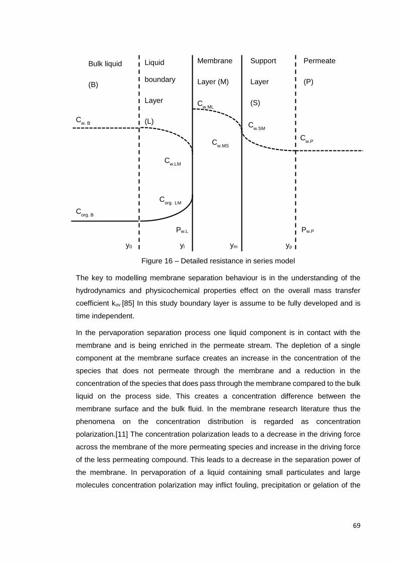
69

The key to modelling membrane separation behaviour is in the understanding of the

hydrodynamics and physicochemical properties effect on the overall mass transfer

coefficient kov [85] In this study boundary layer is assume to be fully developed and is

time independent.

In the pervaporation separation process one liquid component is in contact with the

membrane and is being enriched in the permeate stream. The depletion of a single

component at the membrane surface creates an increase in the concentration of the

species that does not permeate through the membrane and a reduction in the

concentration of the species that does pass through the membrane compared to the bulk

liquid on the process side. This creates a concentration difference between the

membrane surface and the bulk fluid. In the membrane research literature thus the

phenomena on the concentration distribution is regarded as concentration

polarization.[11] The concentration polarization leads to a decrease in the driving force

across the membrane of the more permeating species and increase in the driving force

of the less permeating compound. This leads to a decrease in the separation power of

the membrane. In pervaporation of a liquid containing small particulates and large

molecules concentration polarization may inflict fouling, precipitation or gelation of the

Corg. B

Cw. B

Cw.LM

Corg.

LM

Cw.ML

Cw.MS

Cw.SM

Cw.P

Bulk liquid

(B)

Liquid

boundary

Layer

(L)

Membrane

Layer (M)

Support

Layer

(S)

Permeate

(P)

Figure 16 – Detailed resistance in series model

Pw.P Pw.L

y0 yl ym yp

70

rejected compound on the membrane surface. This in turn, results in a slower permeation

flux and a decrease in the membrane selectivity.[86, 87]

The concentration polarization process can be analysed mathematically. In the liquid

boundary layer the water flux, JvCw,P, is equal to the convective flux, JvCw, and diffusive

flux,-Dw(dCw/dδl). This leads to a mass balance expression, Equation 33.[88]

𝐽𝑣𝐶𝑤 − 𝐷𝑊

𝑑𝐶𝑤

𝑑𝑦𝑙= 𝐽𝑣𝐶𝑤,𝑃

Equation 33

Equation 33 can be integrated across the liquid boundary layer to give Equation 34

known as concentration polarization equation.

𝐶𝑤,𝐿𝑀 − 𝐶𝑤,𝑃

𝐶𝑤,𝐵 − 𝐶𝑤,𝑃= exp(𝐽𝑣𝑦𝑙/𝐷𝑊)

Equation 34

Where Cw,LM is the concentration of water at the membrane surface, Cw,P is the

concentration of water in the permeate and Cw,B is water concentration in the bulk

solution; Jv is volumetric permeation flux (m3 m-2s-1), yl is liquid boundary layer film

thickness (m) and DW is the diffusion coefficient (m2 s-1). An alternative form of the

concentration polarization equation replaces concentration terms with enrichment factors

E defined as Cw.P/Cw.B and E0, an enrichment present without liquid boundary layer,

defined as Cw.P/Cw.LM, also called an intrinsic enrichment factor.[88] The concentration

polarization expression is then rewritten as Equation 35.

1𝐸0

− 1

1𝐸 − 1

= exp(𝐽𝑣𝑦𝑙/𝐷𝑊)

Equation 35

In the pervaporation process, the enrichment factor is larger than unity. This implies that

minor component in the solution is being depleted at the membrane surface and is

selectively permeating to another side. The ratio of the concentration of the permeating

species at the membrane surface and the bulk solution Cw.LM/Cw.B is called polarization

modulus. When concentration polarization modulus is 1 there is no concentration

polarization present. If the modulus deviates from unity, its effect on the pervaporation

flux and selectivity becomes important. Rearrangement of the Equation 34 and Equation

35 leads to Equation 36.

71

𝐶𝑤.𝐿𝑀

𝐶𝑤.𝐵=

𝑒(

𝐽𝑣𝑦𝑙𝐷𝑊

)

1 + 𝐸0(𝑒(

𝐽𝑣𝑦𝑙𝐷𝑊

)− 1)

Equation 36

𝑃𝑒 = 𝐽𝑣𝑦𝑙

𝐷𝑤

Equation 37

Equation 36 shows factors involved in the concentration polarization: i) boundary layer

thickness (𝑦𝑙), volumetric pervaporation flux (Jv), and diffusion coefficient Dw. A change

in any of these variables will affect the concentration polarization. The expression can

be simplified by introducing Peclet number in the exponential term, Equation 37.

The easiest way to control the concentration polarization is to change the liquid boundary

layer thickness. As the liquid boundary layer thickness, yl, decreases the polarisation

modulus decreases exponentially, Equation 36. The liquid boundary can be decreased

by increasing turbulent mixing at the membrane surface. In the membrane module

design the increase in the turbulence is achieved via an increase in the fluid velocity.

Other techniques involve placing a membrane spacer to promote mixing or pulsing the

feed solution. [89, 90]

The concentration polarization is also linked to the membrane selectivity. If the

membrane is completely unselective, E0 = 1, the concentration at the membrane surface

and the components passing through the membrane does not change. In turn,

concentration polarization layer is not generated.

The balance between the convective and diffusive transport in the liquid boundary is

characterised by Jvyl/Dw. This term is a ratio of the convective transport, Jv, and diffusive

transport, yl/Dw, and is commonly referred as the Peclet (Pe) number in the research

literature.[83] By varying the Peclet number and an enrichment factor for a hypothetical

membrane separation process a degree of concentration polarization can be calculated.

The extent of the concentration polarization for a given Pe number and an intrinsic

enrichment factor is shown in Figure 17. As expected, in a process where liquid boundary

layer is thicker or diffusion is lower the concentration polarization is larger. In addition,

an increase in the total permeate flux depletes more permeating species at the

membrane surface faster, thus it can also contribute towards the increase of the

concentration polarization. At high Pe numbers >10 the concentration polarization

reaches its maximum (1/E0) value.

72

Figure 17 - Concentration polarization [83]

2.3.1 Liquid and membrane layer concentration polarization

A general solution of the mass transfer through a liquid boundary layer and a membrane

can be expressed by two second order differential mass balance equations Equation 38,

Equation 39.

Where v is convective velocity (m s-1). After integration of Equation 38, Equation 39 the

concentration distribution in the liquid and membrane boundary layers respectively is

then given by Equation 41 and Equation 45.

To solve 2nd order linear homogenous differential Equation 38 it was assumed that the

solution was proportional to exponential function, Equation 40.

𝐶𝑤 = 𝑒𝜆𝑦 Equation 40

Using the exponential function assumption differential mass transport equations were

solved as follows:

𝑣𝑑

𝑑𝑦𝑙(𝑒𝜆𝑦) − 𝐷𝑤

𝑑2

𝑑𝑦𝑙2 (𝑒𝜆𝑦) = 0

1.00E-05

1.00E-04

1.00E-03

1.00E-02

1.00E-01

1.00E+00

1.00E-06 1.00E-05 1.00E-04 1.00E-03 1.00E-02 1.00E-01 1.00E+00 1.00E+01

Cw

.sm

/Cw

.B

Peclet number (Pe)

E0 = 1 E0 = 10 E0 = 100 E0 = 1000 E0 = 10000 E0 = 100000

𝑣𝑑𝐶𝑤

𝑑𝑦𝑙− 𝐷𝑤

𝑑2𝐶𝑤

𝑑𝑦𝑙2 = 0 0 ≤ 𝑦 ≤ 𝑦𝑙

Equation 38

𝐷𝑤.𝑚

𝑑2𝐶𝑤.𝑀

𝑑𝑦𝑚2 = 0 𝑦𝑙 ≤ 𝑦 ≤ 𝑦𝑙 + 𝑦𝑀

Equation 39

73

The differential terms are then evaluated:

𝑑

𝑑𝑦𝑙(𝑒𝜆𝑦) = 𝜆𝑒𝜆𝑦 and

𝑑2

𝑑𝑦𝑙2 (𝑒𝜆𝑦) = 𝜆2𝑒𝜆𝑦

The unknown function parameter, 𝜆, is then expressed found.

𝑣𝜆𝑒𝜆𝑦 − 𝐷𝑤𝜆2𝑒𝜆𝑦 = 0

𝑒𝜆𝑦(𝑣𝜆 − 𝐷𝑤𝜆2) = 0

𝜆 = 0 or 𝜆 =𝑣

𝐷𝑤

Once the unknown parameter, 𝜆, is expressed full concentration expression can be

written, .

𝐶𝑤.𝐵 = 𝑌1 e𝑣𝑦𝐷𝑤 + 𝑌2 0 ≤ 𝑦 ≤ 𝑦𝑙

Equation 41

Equation 42 describes mass transport in the membrane layer.

𝐷𝑤.𝑚

𝑑2𝐶𝑤.𝑀

𝑑𝑦𝑚2 = 0 𝑦𝑙 ≤ 𝑦 ≤ 𝑦𝑙 + 𝑦𝑀

Equation 42

If the concentration is assumed to be proportional to an exponential function, Equation

43.

𝐶𝑤.𝑀 = 𝑒𝜆𝑦 Equation 43

The mass transport equation has only single answer to the variable

𝐷𝑤.𝑚𝜆2𝑒𝜆𝑦 = 0

𝜆2 = 0

The general solution to a differential equation with a repeated root is, Equation 44.

𝐶𝑤.𝑀 = 𝑌𝑀1𝑦𝑒𝜆𝑦 + 𝑌𝑀2𝑒𝜆𝑦 Equation 44

The final form of the developed Equation 42 is then Equation 45.

𝐶𝑤.𝑀 = 𝑌𝑀1𝑦 + 𝑌𝑀2 𝑦𝑙 ≤ 𝑦 ≤ 𝑦𝑙 + 𝑦𝑀 Equation 45

Where Y1 and Y2 are general solution constants of the liquid boundary layer and YM1 and

YM2 are general solution constants of the membrane layer. To solve the equations,

boundary conditions have to be applied, which lead to Equation 46, Equation 47,

Equation 48 and Equation 49.[91]

𝑌1 + 𝑌2 = 𝐶𝑎𝑞.𝐵 at 𝑦 = 0 Equation 46

𝑣 ∗ 𝑌2 = −𝐷𝑀 ∗ 𝑌𝑀1 at 𝑦 = 𝑦𝑙 Equation 47

74

These equations can be rearranged to give a water flux through the liquid and membrane

layers with respect to a Pe number Equation 50.[11]

𝑄 = 𝑘´𝐿𝑀 ∗ (𝐶𝑤.𝐵𝑒𝑃𝑒 −𝐶𝑤.𝑀𝑆

𝐾𝑆𝐿 )

Equation 50

Where

1

𝑘´𝐿𝑀=

1

𝑘´𝐿 ∗ 𝑃𝑒𝑒𝑃𝑒 − 1

+1

𝑘´𝑀𝐾𝑆𝐿

Equation 51

Equation 51 relates overall (liquid boundary layer and the membrane) mass transfer

coefficient to Pe number and the selective component sorption into the membrane

matrix.[91] The significance of this expression is the relationship between the Pe number

and the combined mass transfer coefficient, kLM.

The concentration polarization, Cw,LM/Cw,B, for a pervaporation process modelled using

liquid and membrane transport phenomena is shown in Equation 52.

𝐶𝑤.𝐿𝑀

𝐶𝑤.𝐵=

𝑁𝑒𝑃𝑒 + (𝑒𝑃𝑒 − 1)𝐶𝑤,𝑃/(𝐶𝑤,𝐵𝐾𝑆𝐿)

𝑒𝑃𝑒 − 1 + 𝑁

Equation 52

Where,

𝑁 = 𝑘´𝑙𝑃𝑒

𝑘´𝑚𝐾𝑆𝐿 =

𝐽𝑣

𝑘´𝑚𝐾𝑆𝐿

Equation 53

The difference between concentration polarization expression Equation 36 and Equation

52 is the intrinsic enrichment factor. In the Equation 36 the intrinsic enrichment factor

has to be assumed, while Equation 52 does not require the intrinsic enrichment factor,

which generally is not known. [91] The permeate concentration on the vacuum side is

often also not known. However, relatively low pressure, < 5mbar, is usually applied,

which makes permeate water concentration tend to decrease close to zero value.

The concentration polarization with respect to changing Pe number and assumed N

value is shown in Figure 18. The polarization decreases with the decrease in the Pe

number. A decrease in the N value leads to an increase in polarization, which means

that an increase in the membrane permeability or an increase in the Henry coefficient

(permeating component solubility in the membrane matrix) creates a more polarized

boundary layer.

𝐾𝑆𝐿(𝑌1 exp 𝑃𝑒 + 𝑌2) = 𝑌𝑀1 ∗ 𝛿𝑀 + 𝑌𝑀2 at 𝑦 = 𝑦𝑙 Equation 48

𝑌𝑀1(𝑦 + 𝑦𝑀) + 𝑌𝑀2 = 𝐶𝑀𝑆 at 𝑦 = 𝑦 + 𝑦 Equation 49

75

Figure 18-Concentration Polarization with respect to 𝑁 value[91]

Typically, Pe is in a range of 10-3-10-4 [83], which leads to expression Equation 54.

1

𝑘´𝐿𝑀≈

1

𝑘´𝐿+

1

𝑘´𝑀

Equation 54

2.3.2 Desorption of water at the membrane/support interface and diffusion through

the porous support

Once water passes the semi-permeable membrane the pressure drops to a vacuum level

≈ 5mbar. The permeate molecules evaporate from the membrane/support interface and

proceed to diffuse through a support layer. In the research literature, this step is

considered as fast and does not produce a significant amount of mass transfer

resistance. [92]

In small capillaries gasses can travel one of three ways which is determined by the

Knudsen number Equation 55.[93]

𝑁𝑘𝑛 =𝑦𝑝

𝑟

Equation 55

Three different mass transport mechanistic models are summarised in the

Table 12

76

Table 12-Vapour transport in porous media

Knudsen number Mechanism of flux

𝑁𝑘𝑛 > 10 Knudsen flow

0.01 < 𝑁𝑘𝑛 < 10 Transient flow

𝑁𝑘𝑛 ≤ 0.01 Viscous flow

In this study the support layer has ≈ 0.2µm nominal pore size and is 125µm thick. It is

hard to estimate the tortuosity of the channels to predict a mean free path. However, it

is anticipated that Nkn will be much greater than 10. Therefore, the water vapour transport

mechanism should follow the Knudsen flow model Equation 56.

𝐽 =2

3∗

𝑑𝑝 ∗ 휀

𝑦𝑝 ∗ 𝜒∗ (

8 ∗ 𝑅 ∗ 𝑇

𝜋 ∗ 𝑀)

12

∗𝑀

𝑅 ∗ 𝑇∗ (𝑃𝑤.𝑆𝑀 − 𝑃𝑤.𝑃)

Equation 56

2.3.3 Transport through the vapour boundary layer

The vacuum side is typically set at ≈ 5mbar this leads to an assumption that as soon as

vapour leaves the membrane support it is taken away and thus presents no mass

transport resistance. Typically, this assumption is made by researchers when studying

pervaporation using high vacuum.[92, 94] However, this is not the case when nitrogen

swept gas is applied to remove the permeate vapour.[94]

2.3.4 Combined mass transfer model

Overall pervaporation mass transfer resistance can be considered as a sum of all

resistances in series. By combining Equation 57, Equation 58 and Equation 59 an overall

mass transfer coefficient is derived Equation 60.

𝑅𝐿𝑖𝑞𝑢𝑖𝑑 =1

𝑘´𝐿 ∗ 𝑃𝑒𝑒𝑃𝑒 − 1

Equation 57

𝑅𝑀𝑒𝑚𝑏𝑟𝑎𝑛𝑒 = 𝑘`𝑀 Equation 58

𝑅𝑆𝑢𝑝𝑝𝑜𝑟𝑡 =1

23 ∗

𝑑𝑝 ∗ 휀𝛿𝑠 ∗ 𝜒

∗ (8 ∗ 𝑅 ∗ 𝑇

𝜋 ∗ 𝑀 )

12

∗𝑀

𝑅 ∗ 𝑇

Equation 59

1

𝑅𝑡𝑜𝑡𝑎𝑙=

1

𝑅𝐿𝑖𝑞𝑢𝑖𝑑 + 𝑅𝑀𝑒𝑚𝑏𝑟𝑎𝑛𝑒 + 𝑅𝑆𝑢𝑝𝑝𝑜𝑟𝑡

Equation 60

Using resistance in series model pervaporation flux is then expressed as a product of

the total resistance and the difference of the permeating species concentration.

77

𝐽 =1

𝑅𝐿𝑖𝑞𝑢𝑖𝑑 + 𝑅𝑀𝑒𝑚𝑏𝑟𝑎𝑛𝑒 + 𝑅𝑆𝑢𝑝𝑝𝑜𝑟𝑡∗ 𝐾𝑆

𝐺 ∗ (𝑃𝑤.𝐵 − 𝑃𝑤.𝑃) Equation 61

Equation 61 is a rigorous membrane model mainly because it encapsulates every

parameter involved in the pervaporation phenomena. Furthermore, each resistance can

be changed individually if any of the membrane parameters change. For in depth variable

examination reader is referred to the original publication.[92]

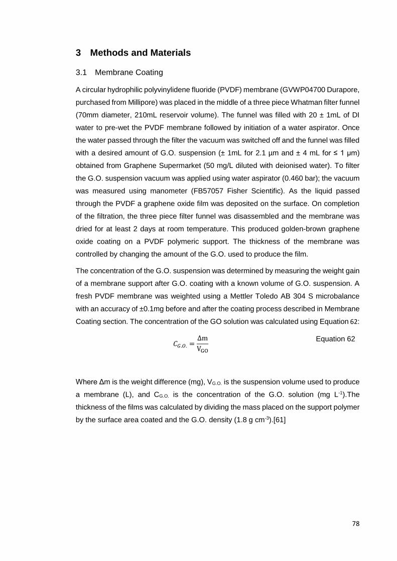
78

3 Methods and Materials

3.1 Membrane Coating

A circular hydrophilic polyvinylidene fluoride (PVDF) membrane (GVWP04700 Durapore,

purchased from Millipore) was placed in the middle of a three piece Whatman filter funnel

(70mm diameter, 210mL reservoir volume). The funnel was filled with 20 ± 1mL of DI

water to pre-wet the PVDF membrane followed by initiation of a water aspirator. Once

the water passed through the filter the vacuum was switched off and the funnel was filled

with a desired amount of G.O. suspension (± 1mL for 2.1 µm and ± 4 mL for ≤ 1 µm)

obtained from Graphene Supermarket (50 mg/L diluted with deionised water). To filter

the G.O. suspension vacuum was applied using water aspirator (0.460 bar); the vacuum

was measured using manometer (FB57057 Fisher Scientific). As the liquid passed

through the PVDF a graphene oxide film was deposited on the surface. On completion

of the filtration, the three piece filter funnel was disassembled and the membrane was

dried for at least 2 days at room temperature. This produced golden-brown graphene

oxide coating on a PVDF polymeric support. The thickness of the membrane was

controlled by changing the amount of the G.O. used to produce the film.

The concentration of the G.O. suspension was determined by measuring the weight gain

of a membrane support after G.O. coating with a known volume of G.O. suspension. A

fresh PVDF membrane was weighted using a Mettler Toledo AB 304 S microbalance

with an accuracy of ±0.1mg before and after the coating process described in Membrane

Coating section. The concentration of the GO solution was calculated using Equation 62:

𝐶𝐺.𝑂. =∆m

VGO

Equation 62

Where Δm is the weight difference (mg), VG.O. is the suspension volume used to produce

a membrane (L), and CG.O. is the concentration of the G.O. solution (mg L-1).The

thickness of the films was calculated by dividing the mass placed on the support polymer

by the surface area coated and the G.O. density (1.8 g cm-3).[61]

79

3.2 Pervaporation Cell

In-house built pervaporation cell (Figure 19 and Figure 20) consists of two chambers,

permeate (1) and process (7), separated by a membrane (5). The process side is fitted

with two 1/16’’ tubes which serve as inlet and outlet. The membrane saddle disk (6) was

designed to accommodate a G.O. membrane and a 1.5 mm thick rubber O-ring (5),

porous stainless steel disk (4) and a perforated stainless steel support (3). Upon

assembly all parts sit at the same height as the top of the membrane saddle disk.

Stainless steel support is then gently compressed by O-rings located in a compression

disk (2). The main core is sandwiched by permeate side (1) and compressed using

screws. The part breakdown is shown in Figure 20. A detailed set of pervaporation cell

drawings is shown in Appendix C.

80

Figure 19 Pervaporation cell computer design

9cm

3cm

0.4cm

0.29cm

5.1cm

9cm

1.2cm

3cm

0.30cm

8.1

9cm

81

Table 13-Pervaporation cell component list

Notation Description

1 Permeate side

2 Compression disk

3 Stainless steel support

4 Porous stainless steel disk

5 G.O. membrane

6 Membrane saddle

7 Process side

1

2 3

4 5

6

7

Figure 20 – Pervaporation cell disassembled view

82

It is important to mention that G.O. membranes are brittle and apparatus must be

assembled with extreme care. Sizeable applied force deviations around the membrane

produce cracks on the periphery. The quality of the membrane surface and the seal

around can be quickly checked by applying vacuum on the permeate side. If a vacuum

cannot be produced the membrane in use most likely has a crack inflicted by an over

tightening the pervaporation cell.

3.3 General Procedure

The pervaporation setup diagram used in all experiments is shown in Figure 21, an

image of a laboratory pervaporation setup is shown in Figure 22. The experimental setup

was composed: i) a conical flask (250 mL) which was used as a feed tank (T1) ii) a pump

P1, (Knauer Smartline two piston pump) to circulate the fluid through the cell, iii) a back

pressure regulator BPR (2.8-5.2 bar) was used to keep the system from boiling, (iv) in-

house developed agitated stainless steel pervaporation cell PERVAP (74 mL, 9.1 cm2

active membrane surface area). Agitation in the cell was provided by a magnetic stirrer

bar rotating at 900 rpm and iv) the permeate side was connected to two cold traps TRAP1

and TRAP2 which were set up in parallel allowing two separate vacuum lines to be open

independently, which ensured continuous operation. Liquid nitrogen was used as a

cooling liquid for the permeate condensation (-195°C). The vacuum side pressure was

set at <5 mbar at all times using vacuum pump P2, (EDWARDS RV3).

A conical flask, T1, was filled with the desired amount and composition solution ±2 mL

followed by an initiation of vacuum on a permeate side using EDWARDS RV3 vacuum

pump, P2. Once < 5mbar pressure was reached on the vacuum side of the pervaporation

cell the process fluid pump (P1) was used to fill the process side with the solution of

interest at 15 mL min-1. Fully assembled pervaporation cell was then placed in a hot oil

or water bath set at an experimental temperature. This was followed by approximately 1

hour of pre-equilibrium stage, allowing pervaporation cell to reach process temperature

and pervaporation flux gain steady state. Thereafter, samples were taken every 1-3

hours and water content was determined using the analytical equipment described in the

3.9 section. A detailed description of standard operating procedures (SOP) can be found

in Appendix D.

83

The rate of permeation was measured using the following expression Equation 63.

J =m

A ∆t Equation 63

Where, J is the permeation flux (kg h-1 m-2), A is membrane surface area (m2), and Δt is

a time of pervaporation (h). It is important to note that the pervaporation time interval did

not affect the mass concentration on the process side to a meaningful extent, thus the

concentration can be assumed to be constant unless stated otherwise.

Pervaporation temperature is one of the several critical parameters in a dehydration

process. To keep pervaporation cell isothermal heat transfer has to be adequate to

provide energy for water evaporation. This is investigated by considering a THF

dehydration study at 70 °C, which resulted in one of the highest permeation fluxes in this

pervaporation research.

Table 14-Energy required to evaporate 2.69g of water over 60min of operation

Notation Value

E(Evaporation) (kJ) N/A

ΔH(Evaporation) (kJ kg-1) 2206

m (kg) 0.00269

E(Evaporation) = m ΔH(Evaporation) Equation

64

Table 15-Heat transfer rate from hot oil bath the pervaporation cell

Notation Value

Ė(transfer) (kJ s-1) N/A

U(Overall) (kW m-2K-1), Assumed 0.2

A (m2) 0.0069

ΔT (K), Assumed 2

Ė(transfer) = U(Overall)A(Area)ΔT Equation 65

84

Table 16-Summary of the heat requirements in a pervaporation process

Notation Value

E(Evaporation) (kJ) 5.93

Ė(transfer) (kJ s-1) 0.0028

t (min) 35

A facile calculation of heat transfer shows that for 60min pervaporation operation 35min

are required to provide all the necessary energy to maintain isothermal conditions. Thus,

the transfer rate was deemed to be sufficient.

85

T1 Stock solution

Heater stirrer plate

Heater bath filled with oil

Assembled pervaporation cell with magnetic stirrer bar

Trap 1

Trap 2

Co

nd

ensers

placed

in a

liqu

id N

2

Vacuum

5 mbar

Recycle line

Permeate line

Process liquid

line

TI

Thermocouple

V1

V2

BPR

Back pressure regulator

Liquid pump

P

Vacuum pump

Pervap

P1

Figure 21 – Detailed pervaporation process drawing

86

Pump

Stock Solution

Heater Stirrer Plate

Hot Oil Bath

Temperature

Monitoring

Pervaporation Cell

Three Way Valve 1

Three Way Valve 2

Condenser 1 Condenser 2

Vacuum Line

Liquid Nitrogen Dewar

Figure 22 – Laboratory pervaporation setup

87

3.4 Liquid side mass transfer coefficient study

In the liquid mass transfer coefficient study a general procedure was followed to preload

65 g (65 ± 1 mL) of deionised water and 150 g (190.8 ± 1 mL) IPA resulting in a 30 wt%

water/IPA solution. The temperature was set at 50°C for all experiments. The rate of

agitation (digitally displayed on the heater stirrer plate) was varied between 0 to 900 rpm.

Permeation was measured using three separate membranes. At least 3 samples at each

degree of agitation were taken.

3.5 Water/Organic and Organic/Organic separations

All separation studies of the Water/Organic and Organic/Organic components were

conducted using the general procedure. The following organic solvents were used in this

study: IPA (>99.5wt%, Fischer Scientific), EtOH (HPLC grade, ≥99.8wt%, Sigma

Aldrich), THF (>99.5wt%, Fischer Scientific), MeOH (HPLC grade, ≥99.9wt%, VWR

International), n-Hexane (95wt%, Fischer Scientific). Selected organic solvent and water

were loaded into a conical flask (250 mL) to make up the desired composition mixture

with a total volume of 250 mL. Summary of the experimental conditions investigated is

shown in Table 17. Multiple membranes were used to determine pervaporation

performance at every set of conditions. The supplier and the grade of the chemicals used

is summarised in Table 18.

88

Table 17-Summary of the Water/Organic and Organic/Organic separations

Entry Estimated

membrane (µm)

Component1

(wt%)

Component2 (wt%) Temperature

(°C)

1 0.56-2.1 Water (0-100) IPA (0-100) 50-80

2 1-2.1 Water (30) EtOH (70) 50-80

3 1-2.1 Water (30) THF (70) 50-80

4 2.1 Water (10-30) MeOH (70-90) 60

5 2.1 MeOH (10-60) n-Hexane (40-90) 60-80

Table 18-Materials used in the research

Material Grade Source

Water N/A Deionised

IPA >99.5wt% Fischer Scientific

EtOH ≥99.8wt% Sigma Aldrich

THF >99.5wt% Fischer Scientific

MeOH ≥99.9wt% VWR International

n-Hexane 95wt% Fischer Scientific

89

3.6 Peptide dewatering

Peptide dewatering study was conducted following the general pervaporation procedure.

In this series of experiments 100 ±1 mL of the selected peptide type and concentration

was loaded into a 100 ±1 mL measuring cylinder. During pervaporation process the

reduction in the solution volume was compensated by adding DI water amount matching

that of the permeate.

In experiments where peptide solution had to be pre-concentrated water was removed

using a Heidolph rotary evaporator. The concentrated solution was then used in a

pervaporation experiment as described above. Summary of the materials used is shown

in Table 19, pervaporation experimental condition are summarised in Table 20.

Table 19-Materials used in the peptide dewatering process

Material Initial concentration

Solids in water (wt%)

Source

Peptide 1 2-8 Industrial Product

Peptide 2 5 Industrial Product

Peptide 3 2 Industrial Product

Table 20-Summary of the peptide dewatering experiments

Peptide

Concentration

(wt%)

Temperature

(°C)

Peptide 3 (pH = 5.5) 2 70

Peptide 1 (pH = 4) 2 80

Peptide 2 (pH = 9.8) 5 80

90

3.7 Esterification

A 2.1 µm G.O. membrane was prepared as described in the Membrane Coating section.

The membrane was placed in a pervaporation cell followed by a full assembly of the

apparatus. A vacuum pump (EDWARDS RV3) was initiated, which produced <5 mbar

pressure on a permeate side. Air leakage through the membrane was tested by

measuring the pressure (FB57057 Fisher Scientific manometer) on the process side 10-

20 min after the initiation of the vacuum pump.

The stock solution vessel was loaded with a 194.96 ± 2 mL (0.719 mol) of long chain

carboxylic acid (Croda Product) and 55 ± 1 mL (0.7919 mol) of IPA at room temperature.

The liquid was thoroughly mixed followed by addition of 2.05 ± 0.01 g of p-toluenesulfonic

acid catalyst. When catalyst was completely dissolved in the reaction mixture the liquid

was loaded into a pervaporation cell at room temperature using two piston pumps

(Knauer Smartline). Once the liquid was circulating the pervaporation cell was placed in

a pre-heated (100°C) hot oil bath with agitation set at 1200 rpm; the stock solution was

placed on a stirrer plate set at 300 rpm without heating.

The reaction was analysed by taking 1 ±0.03 mL of stock solution using 0.5-5 mL

Eppendorf pipette. The drawn reaction mixture was immediately placed in a 30 mL room

temperature IPA loaded with phenolphthalein indicator. The reaction mixture was titrated

dropwise with a 0.1 M NaOH aqueous solution and the amount of titrant required to

induce a colour change was recorded. The analysis was conducted at the start of every

experiment and every hour afterwards.

3.8 Material characterisation

3.8.1 FT-IR

Surface functional groups were determined using an Alpha Bruker spectrometer

(Platinum ATR). Prior to the use of the spectrometer the scanning window was

thoroughly cleaned with dichloromethane. A sample was placed on an ATR window and

clamped down. At least three runs at different membrane locations were taken with each

spectra composed of 16 scans which were averaged. Between every sample

measurement the equipment was cleaned and background was rescanned.

In preparation of the ATR all membranes were washed with DI water and IPA.

Membranes were allowed to dry for at least 4 days at room temperature unless stated

otherwise.

91

A G.O. only sample was prepared by removing water with a rotary evaporator from highly

concentrated G.O. solution (5 g L-1, 0.5-5 µm flake size, 79 wt% Carbon, 21 wt% Oxygen,

>60% single sheets) purchased from Graphene-Supermarket.

3.8.2 Thermal Properties

Thermal properties were studied using DSC (TA instruments Q20) and TGA (TA

instruments, Q50). The samples were weighted using Mettler Toledo (AB304-s)

microbalance (±1mg). Both analyses were conducted at a 5°C min-1 heating rate.

3.8.3 SEM and EDX

Visual analysis of the G.O. membrane was performed using SEM (Hitachi SU8230

coupled with Oxford instruments Aztec EDX). A small piece of used G.O. membrane was

ascertained by cracking the membrane in a liquid nitrogen. The collected samples were

placed on a number of SEM holder plates. One side of the sample was covered by a

carbon glue connecting the surface of the membrane to the metal support of the SEM

holder. All membranes were kept in a desiccator (30 mbar) for at least 4 days prior to

imaging to remove all of the residual solvents.

3.8.4 Contact Angle

Prior to analysis membrane surface was cleaned using DI water and IPA. Clean

membranes were allowed to dry for at least 4 days prior to the contact angle

measurements. In its natural state used G.O. membranes were slightly bent, this was

rectified by gluing the bottom of the G.O. membrane surface (PVDF) onto a glass slide

using double sided tape. Once the measurement device was calibrated a glass slide with

a G.O. membrane was placed on a sample stage and at least 5 drops of DI water were

placed on a surface for the measurements using Cam 200 KSV tensiometer.

92

3.9 Water Analysis

3.9.1 Karl Fischer analysis

Karl Fischer (Mettler Toledo, DL38) was coupled with Hydranal 5 titrant and Hydranal

solvent (Fluka analytical). The apparatus had 5 mL burette capable of analysing water

content in a range of 1-100 wt%. Prior to analysis the equipment was calibrated using

100 mg of DI water or 1 mL of Hydranal Water Standard 10 (1 wt% water in an organic

solvent). The calibration samples and permeate samples were weighted using Mettler

Toledo (AB304-s) microbalance (±1mg). Every sample was analysed at least three times

and the average was tabulated as a water concentration.

3.9.2 GC analysis

Gas chromatographer (HP6890 Series) was used to determine the concentration of the

organic component. The analytical equipment was equipped with a HP 5 column, 30 m

length, 0.32 mm diameter, and 0.25 µm film thickness. Sample (1 µL at 1:100 split). The

sample was injected at 250°C followed by a hold at 40°C for 5 minutes, the temperature

was then raised by 50°C min-1 to 200°C and held for 1 min.

Prior to the analysis of the permeate samples a calibration curve was prepared.

Permeate sample organic component response area was then compared against the

calibration curve and the amount of the organic compound was ascertained. From this

result water concentration in the permeate was calculated.

3.9.3 Refractometer

Water concentration in the permeate was also measured using refractive index using a

refractometer (Bellingham and Stanley). Several drops of the permeate were placed on

the refractometer glass which then clamped with a metal lid at room temperature. The

concentration was determined by measuring the deviation of the refractive index from

the 1.3333 value.

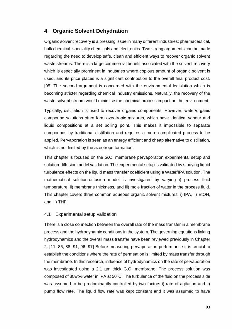
93

4 Organic Solvent Dehydration

Organic solvent recovery is a pressing issue in many different industries: pharmaceutical,

bulk chemical, speciality chemicals and electronics. Two strong arguments can be made

regarding the need to develop safe, clean and efficient ways to recover organic solvent

waste streams. There is a large commercial benefit associated with the solvent recovery

which is especially prominent in industries where copious amount of organic solvent is

used, and its price places is a significant contribution to the overall final product cost.

[95] The second argument is concerned with the environmental legislation which is

becoming stricter regarding chemical industry emissions. Naturally, the recovery of the

waste solvent stream would minimise the chemical process impact on the environment.

Typically, distillation is used to recover organic components. However, water/organic

compound solutions often form azeotropic mixtures, which have identical vapour and

liquid compositions at a set boiling point. This makes it impossible to separate

compounds by traditional distillation and requires a more complicated process to be

applied. Pervaporation is seen as an energy efficient and cheap alternative to distillation,

which is not limited by the azeotrope formation.

This chapter is focused on the G.O. membrane pervaporation experimental setup and

solution-diffusion model validation. The experimental setup is validated by studying liquid

turbulence effects on the liquid mass transfer coefficient using a Water/IPA solution. The

mathematical solution-diffusion model is investigated by varying i) process fluid

temperature, ii) membrane thickness, and iii) mole fraction of water in the process fluid.

This chapter covers three common aqueous organic solvent mixtures: i) IPA, ii) EtOH,

and iii) THF.

4.1 Experimental setup validation

There is a close connection between the overall rate of the mass transfer in a membrane

process and the hydrodynamic conditions in the system. The governing equations linking

hydrodynamics and the overall mass transfer have been reviewed previously in Chapter

2. [11, 86, 88, 91, 96, 97] Before measuring pervaporation performance it is crucial to

establish the conditions where the rate of permeation is limited by mass transfer through

the membrane. In this research, influence of hydrodynamics on the rate of pervaporation

was investigated using a 2.1 µm thick G.O. membrane. The process solution was

composed of 30wt% water in IPA at 50°C. The turbulence of the fluid on the process side

was assumed to be predominantly controlled by two factors i) rate of agitation and ii)

pump flow rate. The liquid flow rate was kept constant and it was assumed to have

94

negligible effects on the total fluid turbulence in the presence of agitation. Furthermore,

the liquid concentration was kept constant by replenishing the depleted water in the

process solution by adding fresh DI water. It was assumed that the pervaporation was

not heat transfer limited as the amount of water permeating was small (1 – 2g) and the

operation time was between 1 – 2 hours.

To study the effects of turbulence on the permeation the rate of agitation was altered.

The rate of permeation was plotted as a function of agitation as shown in Figure 23. The

rate of permeation gradually increased from an average value of 0.16 kg h-1 m-2 to 0.73

kg h-1 m-2 while increasing the RPM from 0 to 550 respectively. The increase was

associated with the shifting rate of mass transfer limiting step. At a low rate of agitation,

the rate of pervaporation was dominated by the liquid side mass transfer coefficient. As

the rate of agitation was increased the liquid side mass transfer boundary layer shrank.

[95] At higher rates of agitation (>550 RPM) the rate of permeation has gained a steady

value of ≅ 0.74 kg h-1 m-2. This marked a region where the rate of permeation was limited

by the membrane mass transfer coefficient, an inherent property of the material. It is

impossible to completely eliminate the liquid side mass transfer coefficient and even in

completely turbulent conditions a laminar sub layer exists. [95] However, in the region of

high agitation (>550 RPM) it was assumed that the liquid mass transfer coefficient

becomes insignificant. The resistance of the porous support layer was also assumed to

be insignificant.

Figure 23-Pervaporation flux change with respect to the change in agitation, water/IPA

(30 / 70wt%), 50°C, 2.1μm.

0

10

20

30

40

50

60

70

80

90

100

0

0.1

0.2

0.3

0.4

0.5

0.6

0.7

0.8

0.9

1

0 200 400 600 800 1000

Per

mea

te P

uri

ty (

wt%

)

Flu

x (k

g h

-1m

-2)

Rotations per minute (RPM)

Permeation Flux Permeate Purity

Membrane and liquid mass

transfer controlled region

Membrane controlled mass

transfer region

95

To calculate individual mass transfer coefficients of the pervaporation process, several

assumptions are made: high agitation region (>550 rpm) is controlled by the membrane

mass transfer, thus the liquid boundary layer resistance becomes irrelevant and cannot

be separately determined. This assumption simplifies previously shown resistance in

series model to Equation 66

𝐽 =1

𝑅𝑀𝑒𝑚𝑏𝑟𝑎𝑛𝑒𝐾𝑠

𝐺(𝑃𝑤.𝐿 − 𝑃𝑤.𝑃) = 𝑘𝑚.𝑝(𝑃𝑤.𝐿 − 𝑃𝑤.𝑃) Equation 66

𝑘𝑚.𝑝 = 𝐷𝑤𝑚

𝐾𝑠𝐺

𝑦𝑚

Equation 67

Where, km.p is membrane mass transfer coefficient (kg bar-1s-1m-2),ym is membrane

thickness (m) and Dwm is effective water diffusion coefficient in the membrane matrix (m2

s-1) KSG is gas sorption coefficient (kg bar-1m-3).

To determine conventional mass transfer coefficient, the water vapour partial pressure

term is replaced by mass concentration as a driving force. The expression is then further

simplified by ignoring the water concentration on the permeate side resulting in a final

expression Equation 68. The simplified expression was then used to calculate membrane

mass transfer resistance.

𝐽 =𝐷𝑤𝑚

𝐾𝑠𝐿

𝑦𝑚ρw,LM

L = 𝑘`𝑚ρw,LML

Equation 68

Where, KsL is liquid partition coefficient (dimensionless), 𝑘`𝑚 is membrane mass transfer

coefficient (m s-1), and ρw,LM is water concentration in the bulk solution (kg m-3). For the

ease of calculation, the liquid partition coefficient from here onwards is combined with

the mass transfer coefficient.

At the lower rates of agitation (<550 rpm) the liquid boundary layer becomes a large part

of the overall resistance and thus can no longer be ignored. The pervaporation flux

96

equation then has to be extended to include liquid boundary layer resistance Equation

69.

𝐽 =1

1𝑘`𝑙

+𝑦𝑚

𝐷𝑤𝑚

ρw,LM =1

1𝑘`𝑙

+1

𝑘`𝑚

ρw,LML = 𝑘𝑜𝑣ρw,LM

L Equation 69

When the overall and the membrane mass transfer coefficients are known the liquid

boundary layer mass transfer coefficient can be calculated using

𝑘`𝑙 =𝑘`𝑜𝑣𝑘`𝑚

𝑘`𝑚 − 𝑘`𝑜𝑣

Equation 70

Water mass transport coefficients in the liquid and membrane layers were calculated

from experimental data and are shown in Table 21. It is interesting to note that the initial

research has pointed out that G.O. membrane held no resistance to water diffusion.[1]

Unfortunately, this was only an interpretation of limited pervaporation experimental data.

The water mass transfer coefficient in the membrane matrix at 50°C is of a typical

magnitude found in pervaporation processes. Water diffusion in the liquid boundary layer

was also of a similar value found in the previous diffusion research.[98] The distribution

of the mass transfer coefficients show a very strong influence of a water boundary layer

resistance when no agitation is present.as the agitation is increased the liquid boundary

layer mass transfer coefficient increases from 2.21*10-7 m s-1 to 2.75*10-5 m s-1and

presents only 3% resistance to the overall mass transfer in a pervaporation operation.

Table 21- Mass transfer coefficients, water/IPA (30 / 70wt%), 50°C, 2.1μm.

Agitation

(rpm)

Flux

(kg h-1m-2)

k`ov x10-7

(m s-1)

k`m x10-7

(m s-1)

Resistance

(%)

k`l x10-7

(m s-1)

Resistance

(%)

0 0.16 1.74 8.24 21.14 2.21 78.86

250 0.43 4.67 8.24 56.68 10.78 43.32

500 0.73 8.00 8.24 97.09 274.6 2.91

97

It is frequently suggested that it is important to continue making ever thinner

pervaporation membranes.[15, 17, 58, 99] However, the liquid boundary layer mass

transfer limitation is often not considered at the membrane design stage. Assuming the

liquid boundary layer mass transfer coefficient stays constant and the membrane mass

transfer coefficient reduces linearly with a decrease in the membrane thickness. It is

possible to calculate how thin the G.O. membrane can be until the liquid boundary layer

resistance starts dominating the mass transfer process. The membrane mass transfer

resistance contribution to the overall mass transfer process at different membrane

thicknesses is shown in Figure 24. A hypothetical pervaporation process is dominated

by the membrane mass transfer from 2.1 to 1µm membrane thickness. At a smaller

membrane thicknesses liquid boundary layer resistance has a significant contribution.

Up to date, the thinnest G.O. membrane tested in a commercial pervaporation unit had

0.097µm thick selective layer.[100] If the membrane would be used in this experiment

the liquid boundary layer resistance contribute 39% of the total resistance.

Figure 24- Mass transfer resistance (%) change with respect to the change in membrane

thickness, water/IPA (30 / 70wt%), 50°C, 2.1 – 0.01μm

0

5

10

15

20

25

0

20

40

60

80

100

0 0.5 1 1.5 2 2.5

Flu

x (k

g h

-1m

-2)

G.O

. mem

bra

ne

resi

stan

ce (

%)

Membrane thickness (µm)

Membrane Resistance Pervaporation Flux

98

An empirical methodology used to validate the performance of pervaporation equipment

is well known.[11] However, the transferability of the liquid side mass transfer coefficient

expression is very limited. A similar curve at identical conditions will be obtained only in

a similar geometry and size pervaporation cell. A significantly different pervaporation cell

design, would require a repeat of all experiments to determine a new membrane limited

mass transfer zone.

4.2 G.O. membrane long term performance

The stability of the G.O. membrane was investigated by exposing a 2.1 µm thick G.O.

membrane to a 20wt% water in IPA solution at 80°C for 40 hours. The entire study was

subdivided into a 7-day consecutive pervaporation experiments. The average and

measured values of the permeation flux and permeation purity are shown in Figure 25.

The measured pervaporation flux values were scattered probably due to the temperature

fluctuations and sample extraction error; thus, the permeation rates were averaged. The

declining trend became apparent. During the entire course of the study permeation flux

has declined from an average value of 1.28 to 0.82 kg h-1 m-2, which corresponds to a

loss of 36 % of permeation rate, Figure 26. The permeate purity produced an inclining

trend and remained very high in the region of 95.2-99.0 wt%.

Figure 25-Membrane stability over 7 day period, water/IPA (20 / 80wt%), 80°C, 2.1μm.

90

91

92

93

94

95

96

97

98

99

100

0

0.2

0.4

0.6

0.8

1

1.2

1.4

0 4 8 12 16 20 24 28 32 36 40 44

Per

mea

te P

uri

ty (

wt%

)

Flu

x (k

g h

-1m

-2)

Time (h)

Permeation Flux Permeation Flux (Average) Permeate Purity

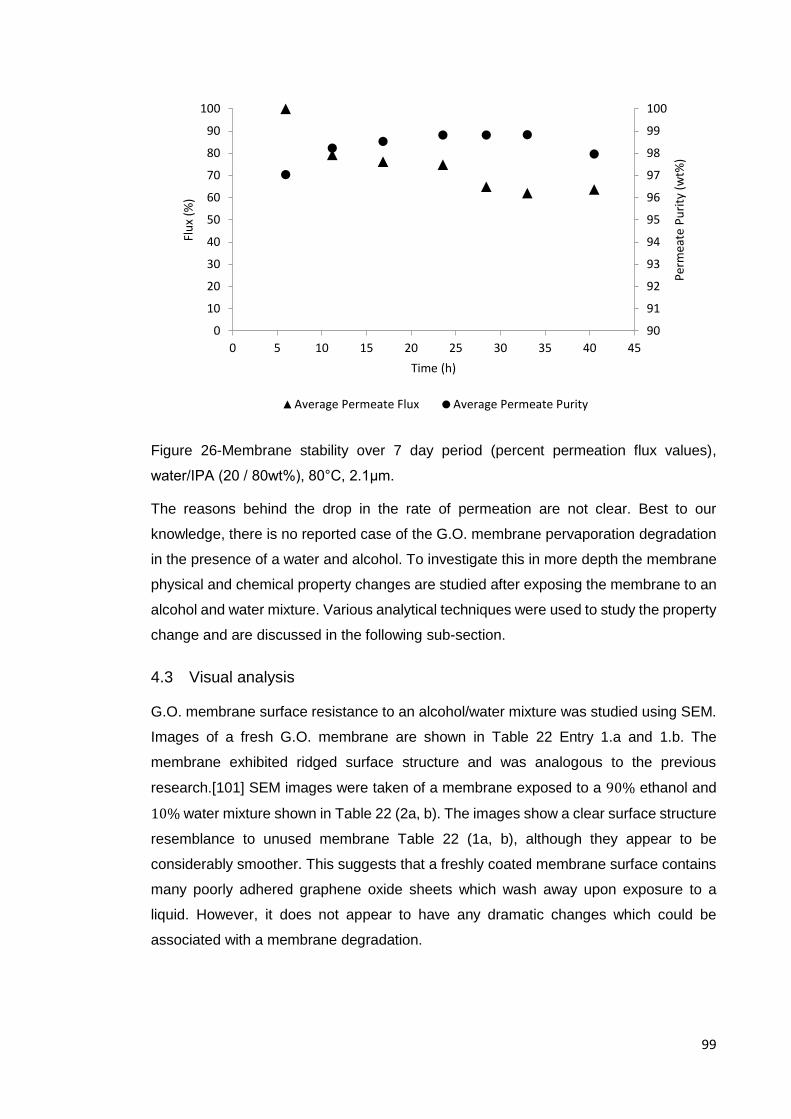
99

Figure 26-Membrane stability over 7 day period (percent permeation flux values),

water/IPA (20 / 80wt%), 80°C, 2.1μm.

The reasons behind the drop in the rate of permeation are not clear. Best to our

knowledge, there is no reported case of the G.O. membrane pervaporation degradation

in the presence of a water and alcohol. To investigate this in more depth the membrane

physical and chemical property changes are studied after exposing the membrane to an

alcohol and water mixture. Various analytical techniques were used to study the property

change and are discussed in the following sub-section.

4.3 Visual analysis

G.O. membrane surface resistance to an alcohol/water mixture was studied using SEM.

Images of a fresh G.O. membrane are shown in Table 22 Entry 1.a and 1.b. The

membrane exhibited ridged surface structure and was analogous to the previous

research.[101] SEM images were taken of a membrane exposed to a 90% ethanol and

10% water mixture shown in Table 22 (2a, b). The images show a clear surface structure

resemblance to unused membrane Table 22 (1a, b), although they appear to be

considerably smoother. This suggests that a freshly coated membrane surface contains

many poorly adhered graphene oxide sheets which wash away upon exposure to a

liquid. However, it does not appear to have any dramatic changes which could be

associated with a membrane degradation.

90

91

92

93

94

95

96

97

98

99

100

0

10

20

30

40

50

60

70

80

90

100

0 5 10 15 20 25 30 35 40 45

Per

mea

te P

uri

ty (

wt%

)

Flu

x (%

)

Time (h)

Average Permeate Flux Average Permeate Purity

100

Table 22 - Visual G.O. Characterisation

Experiment

Reference.

Conditions and

comments

SEM image

1.a Fresh membrane

(0.21 𝑚𝑔/𝑐𝑚2)

magnified 500 times.

1.b Fresh membrane

(0.21 𝑚𝑔/𝑐𝑚2)

magnified 5000 times.

2a A G.O. membrane

exposed to ethanol

water mixture for

several hours in a

pervaporation cell.

Note sharp looking

ridges smoothed out.

Magnified 500 times

2.b A G.O. membrane

exposed to ethanol

water mixture for

several hours in a

pervaporation cell.

Magnified 5000 times

101

4.4 Thermal degradation

Thermal stability of the G.O. is of paramount importance for reliable a membrane

pervaporation performance at elevated temperatures. Naturally, it is desirable to have a

membrane material that is stable over a wide temperature range since typically

pervaporation operations are carried out below 100°C. Thermal stability of the material

was studied using TA instruments DSC (Q20) and TA instruments TGA (Q50).

Figure 27-DSC scan in a 0-500°C temperature range at a 5°C per minute heating rate

Figure 28-TGA scan in a 0-500°C temperature range at a 5°C per minute heating rate

-5

0

5

10

15

0 100 200 300 400 500

Hea

t Fl

ow

Exo

Up

(m

W)

Temperature (°C)

0.4

0.5

0.6

0.7

0.8

0.9

1

0 100 200 300 400 500

Sam

ple

(w

t%)

Temperature (°C)

102

There was approximately 17% mass loss in a 50 – 160°C temperature range with an

endothermic energy peak at 109°C. This mass loss was assigned to the loss of adsorbed

water and a small loss of 𝐶 − 𝑂𝐻 groups. This temperature region is also known to be

favourable for a 𝐶 = 𝑂 group formation in a multi-layered G.O.[102, 103]

An exothermic event in the 160-250°C temperature range resulted in a ≈27% mass with

the event peaking at ≈197°C. This was allocated to a pyrolysis of labile groups resulting

in a 𝐶𝑂 and 𝐶𝑂2 release. The temperature region is known to be favourable for the

formation of 𝐶 = 𝑂, 𝐶 − 𝑂 and a loss of the epoxide, 𝐶 − 𝑂𝐻, and 𝐶𝑂𝑂𝐻 groups.[103]

The remainder of the TGA profile had a much shallower gradient trending downwards.

This was associated with a gradual loss of the following functional groups, 𝐶 −

𝑂, 𝐶𝑂𝑂𝐻, 𝐶 − 𝑂𝐻, and 𝐶 = 𝑂 tightly packed in a G.O. lattice. DCS and TGA profiles were

consistent with previous research reported in the literature. [102, 104-106] [103]

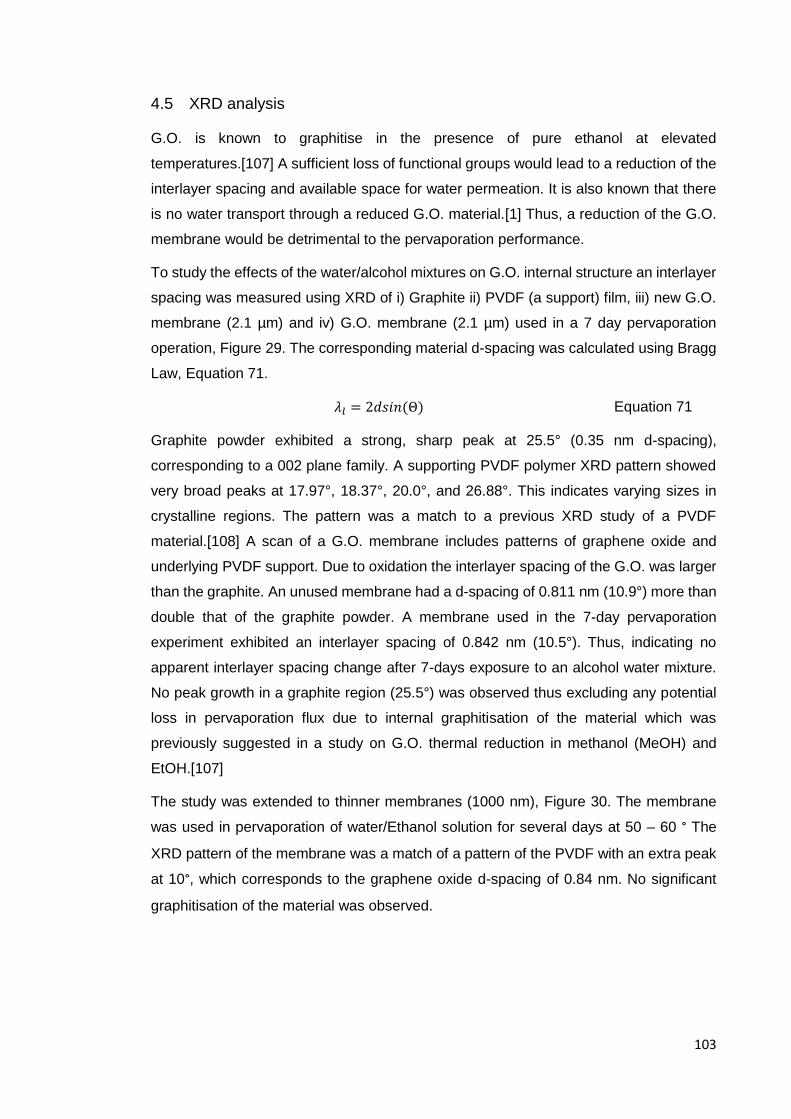
103

4.5 XRD analysis

G.O. is known to graphitise in the presence of pure ethanol at elevated

temperatures.[107] A sufficient loss of functional groups would lead to a reduction of the

interlayer spacing and available space for water permeation. It is also known that there

is no water transport through a reduced G.O. material.[1] Thus, a reduction of the G.O.

membrane would be detrimental to the pervaporation performance.

To study the effects of the water/alcohol mixtures on G.O. internal structure an interlayer

spacing was measured using XRD of i) Graphite ii) PVDF (a support) film, iii) new G.O.

membrane (2.1 µm) and iv) G.O. membrane (2.1 µm) used in a 7 day pervaporation

operation, Figure 29. The corresponding material d-spacing was calculated using Bragg

Law, Equation 71.

𝜆𝑙 = 2𝑑𝑠𝑖𝑛(Θ) Equation 71

Graphite powder exhibited a strong, sharp peak at 25.5° (0.35 nm d-spacing),

corresponding to a 002 plane family. A supporting PVDF polymer XRD pattern showed

very broad peaks at 17.97°, 18.37°, 20.0°, and 26.88°. This indicates varying sizes in

crystalline regions. The pattern was a match to a previous XRD study of a PVDF

material.[108] A scan of a G.O. membrane includes patterns of graphene oxide and

underlying PVDF support. Due to oxidation the interlayer spacing of the G.O. was larger

than the graphite. An unused membrane had a d-spacing of 0.811 nm (10.9°) more than

double that of the graphite powder. A membrane used in the 7-day pervaporation

experiment exhibited an interlayer spacing of 0.842 nm (10.5°). Thus, indicating no

apparent interlayer spacing change after 7-days exposure to an alcohol water mixture.

No peak growth in a graphite region (25.5°) was observed thus excluding any potential

loss in pervaporation flux due to internal graphitisation of the material which was

previously suggested in a study on G.O. thermal reduction in methanol (MeOH) and

EtOH.[107]

The study was extended to thinner membranes (1000 nm), Figure 30. The membrane

was used in pervaporation of water/Ethanol solution for several days at 50 – 60 ° The

XRD pattern of the membrane was a match of a pattern of the PVDF with an extra peak

at 10°, which corresponds to the graphene oxide d-spacing of 0.84 nm. No significant

graphitisation of the material was observed.

104

Figure 29-XRD patterns of i) Graphite, ii) PVDF, iii) New Membrane, and iv) G.O. membrane tested in a 7 day pervaporation process.

Figure 30-XRD patterns of i) Graphite, ii) PVDF, and iii) G.O. Membrane (1 µm)

5 10 15 20 25 30 35 40

Am

plit

ute

(n

orm

alis

ed t

o 1

co

un

ts)

2Θ

Gaphite PVDF New Membrane IPA Test

5 10 15 20 25 30 35 40Am

plit

ute

(n

orm

alis

ed t

o 1

co

un

ts)

2Θ (deg)

Graphite PVDF Membrane (1000 nm)

105

4.6 FT-IR analysis

Numerous authors have studied graphene oxide using IR spectroscopy.[60, 68, 109,

110] Historically, there has been some debate over the peak assignments. The reason

of disagreement is the presence of a very broad peak in a 2800 − 3800 cm-1 range due

to adsorbed water, which in turn can conceal or partially block other peaks.[60]

In this study, G.O., functional groups were investigated using Bruker Alpha ATR-IR

spectrometer, Figure 31. The peak at 2800 – 3800 cm-1 was assigned to a hydroxyl group

stretching and intercalated water molecules.[110] The nature of such a broad peak can

be explained by hydroxyl groups attached to the carbon basal plane in different forms,

such as tertiary and secondary alcohols, enols, phenols and carboxylic groups.[110]

There is a small, shoulder like, peak at 1713 cm-1. This was assigned to the carbonyl

groups present in ketones and carboxylic acids located at the edge of the basal

plane.[68] The peak at 1625 cm-1 originates from un-oxidised aromatic regions in the

structure. The peak at 1218 cm-1 was assigned to the 𝐶 − 𝑂 − 𝐶. The fingerprint region

was composed of 𝐶 − 𝐶 and 𝐶 − 𝑂 bonds. [111]

Figure 31- FT-IR of G.O.

FT-IR was used to investigate the surface changes of the membrane used in an

IPA/Water pervaporation operation for 7 consecutive days. Membrane functional group

changes were assessed against i) G.O. film, ii) new membrane, and ii) PVDF polymeric

support shown in Figure 32. The landscape of the PVDF and G.O. film spectra was a

match to the previous literature data.[110, 112] The spectrum of the new G.O. membrane

was almost a complete match to an unsupported G.O. film. Minute peak differences were

0

0.1

0.2

0.3

0.4

0.5

0.6

0.7

0.8

0.9

1

40080012001600200024002800320036004000

Ab

sorb

ance

(A

.U,)

Wavelength (cm-1)

G.O.

C-O-C

1046 cm-1

C=C

1623 cm-1

O-H

C=O

1723 cm-1

106

observed in the fingerprint region (400 – 900 cm-1), which are most likely resulting from

an underlying PVDF polymeric support. There were no other major differences between

the G.O. film and new G.O. membrane IR spectra. A set of three distinct peaks (2950

cm-1, 2919 cm-1 and 2845 cm-1) was observed in the used membrane FT-IR scan. Peaks

in this region result from C-H stretches (2950-3000 cm-1). The exact same location of the

peaks is present in the IPA spectrum, suggesting that the IPA is present on or in the

membrane. It is not entirely clear whether IPA has permanently bonded to the G.O.

surface or just small amounts of the compound intercalated between the G.O. sheets.

Figure 32-FT-IR of i) G.O, ii) Used Membrane, iii) New Membrane, and iv) PVDF

To rule out the possibility of the additional peaks being an artefact of the intercalated

solvent into the G.O. matrix a fresh membrane was soaked in the IPA solution for 24

hours and dried in a vacuum oven for 9 days at 40°C. FT-IR spectrum of the i) soaked

membrane, ii) fresh membrane, and iii) used membrane is shown in Figure 33. There

were significant changes in the fingerprint region among all of the spectra. No IPA peaks

were observed in the soaked membrane FT-IR scan. This supports the argument that

the IPA has permanently attached to the G.O. surface during pervaporation operation.

40080012001600200024002800320036004000

Ab

sorp

tio

n (

A.U

.)

G.O. Used Membrane New Membrane PVDF

107

Figure 33-FT-IR spectra of i) G.O., ii) Soaked Membrane, and iii) Used Membrane

Membrane surface hydrophilicity affects water partitioning into the membrane matrix,

permanent bonding of the IPA to the surface of the G.O. can change the hydrophilicity

and in turn negatively affect water partitioning. A water droplet contact angle

measurement is an easy and fast way to assess the surface hydrophilicity.[97] If a water

droplet has a contact angle smaller than 90° the surface is said to be hydrophilic (high

wettability), the opposite is true if the

surface contact angle is less than 90°.

Images of a water droplet on a fresh G.O.

membrane and the membrane used in the

7 days dewatering process are shown in

Figure 34 a) and b) respectively. Oxygen

groups on the graphene surface have been

known to introduce a hydrophilic property

to the material. The contact angle of water

on the fresh G.O. surface was 65.88° and

65.63°, confirming the hydrophilic nature of

the surface. The contact angle of a water

droplet on the used membrane surface has significantly increased to 87.14° and 87.47°.

This suggests a large surface chemistry change has taken place during the

pervaporation operation, which has significantly reduced G.O. membrane hydrophilicity.

In light of G.O. material surface chemistry instability at elevated temperatures the

40080012001600200024002800320036004000

Ab

sorp

tio

n (

A.U

.)

Wavelength (cm-1)

G.O. Soaked Membrane Used Membrane

Figure 34 – Water contact angle on the a) fresh G.O. membrane, and b) used G.O. membrane

87.14° 87.47°

65.88° 65.63°

a)

b)

108

increase in the contact angle is most likely the results of the IPA reaction at the

membrane surface and previously reported material thermal degradation. The reduction

in the surface wettability would explain the drop in the rate of permeation over time. As

the membrane becomes less hydrophilic water finds it harder to wet the surface and

intercalate between the G.O. sheets.

4.7 Solution-diffusion model validation

It is accepted that the solution-diffusion model describes pervaporation process,

Equation 72. In this model the transport of the permeating species is a product of the

permeability coefficient and partial pressure difference across the membrane. To get a

detailed view of the membrane material performance, typically pervaporation flux change

with respect to the change in process parameters is studied.

𝐽 =𝐷𝑤𝑚

𝐾𝑠𝐺

𝑦𝐺𝑂𝑥 𝛾10𝐴−

𝐵𝐶+𝑇

Equation 72

From Equation 72, it is apparent that the change in the rate of pervaporation can be

altered in three ways: i) varying temperature of the operation, ii) changing membrane

thickness and iii) varying the mole fraction of water in the process solution. In typical

membrane permeation performance studies pervaporation flux change with respect to

the change in temperature and mole fraction is reported. [15, 71, 73, 100] In this work

the influence of all three variables on the rate of permeation are studied.

4.7.1 Temperature effects

The feed temperature is a crucial variable in a pervaporation process as it influences

both separation quality and flux. To gain an insight into G.O. membrane performance

with respect to the temperature change, three common binary solvent systems were

tested: i) 30wt% Water/IPA, ii) 30wt% Water/EtOH, and iii) 30wt% Water/THF.

Water/IPA solution was tested using a 2.1 µm thick membrane in a temperature range

of 50 – 70 “C. The pervaporation flux through a G.O. membrane was first plotted against

the water vapour partial pressure, Figure 35. The permeate flux increased linearly with

the driving force whilst maintaining the purity of water on the permeate side at high levels;

between 97.9 and 99.5 wt%. In all experiments the observed permeate quality was

considered to be very pure and is of comparable purity with other research or commercial

membranes.[76, 113] The variations in water purity did not follow any trend and were

most likely caused by a variation in the membrane quality.

109

Figure 35-Pervaporation flux of water/IPA (30 / 70wt%) solution at 50, 60, and 70°C,

2.1μm membrane

A binary pair of Water/EtOH was studied in a 50 – 80°C temperature range. As

anticipated the permeation flux rose linearly with increase in partial pressure and was in

agreement with the solution-diffusion model, Figure 36. The permeation flux was

significantly lower when compared to the Water/IPA system. The permeate purity (95.0-

95.7 wt%) was also slightly lower than the Water/IPA binary pair. This was attributed to

the smaller molecular kinetic diameter of the ethanol molecule leading to an easier

intercalation into the G.O. structure and faster permeation rates of the organic species.

A Water/THF solution was investigated in a 50 – 70°C temperature range using a thinner,

1 µm membrane. The permeation flux trend was in agreement with the solution-diffusion

model and increased linearly with increase in partial pressure. As expected, the rate of

permeation was significantly higher due to the thinner membrane. The permeate purity

remained high in the entire temperature envelope at 97.6 – 99.1 wt% water. A perfect

compound separation was anticipated and the presence of the THF in the permeate was

surprising. The permeation was attributed to the imperfections in the membrane surface.

0

10

20

30

40

50

60

70

80

90

100

0

0.2

0.4

0.6

0.8

1

1.2

1.4

1.6

0 0.05 0.1 0.15 0.2 0.25 0.3

Per

mea

te P

uri

ty (

wt%

)

Flu

x (k

g h

-1m

-2)

Partial Pressure (bar)

Pervaporation Flux Permeate Purity

110

Figure 36-Pervaporation of water/ethanol (30 / 70wt%) solution at 50, 60, 70, 80°C, 2.1 µm membrane

Figure 37-Pervaporation of water/THF (30 / 70wt%) solution at 50, 60, 70°C, 1.0 µm membrane

0

10

20

30

40

50

60

70

80

90

100

0

0.2

0.4

0.6

0.8

1

1.2

1.4

1.6

0 0.05 0.1 0.15 0.2 0.25 0.3 0.35 0.4

Per

mea

te P

uri

ty (

wt%

)

Flu

x (k

g h

-1m

-2)



0

10

20

30

40

50

60

70

80

90

100

0

0.5

1

1.5

2

2.5

3

3.5

0 0.05 0.1 0.15 0.2 0.25 0.3

Per

mea

te P

uri

ty (

wt%

)

Flu

x (k

g h

-1m

-2)



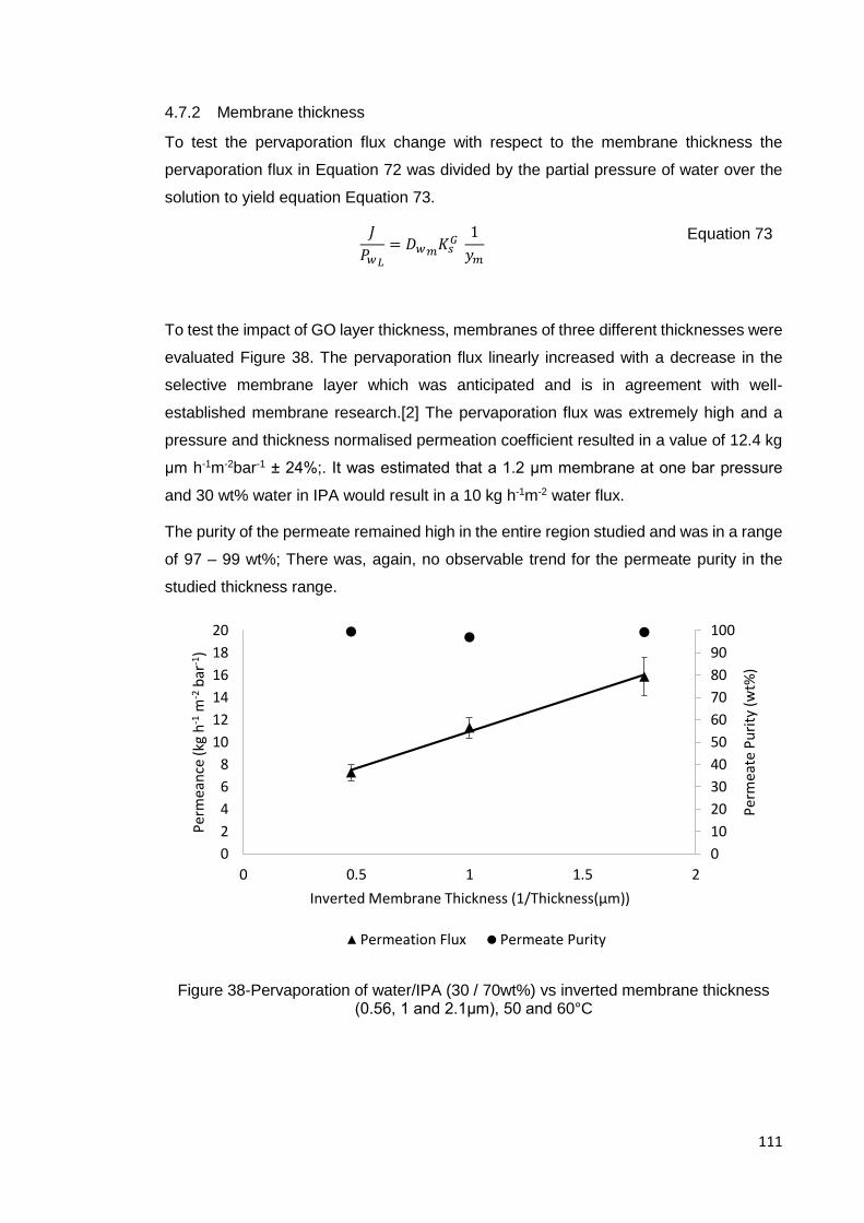
111

4.7.2 Membrane thickness

To test the pervaporation flux change with respect to the membrane thickness the

pervaporation flux in Equation 72 was divided by the partial pressure of water over the

solution to yield equation Equation 73.

𝐽

𝑃𝑤𝐿

= 𝐷𝑤𝑚𝐾𝑠

𝐺 1

𝑦𝑚

Equation 73

To test the impact of GO layer thickness, membranes of three different thicknesses were

evaluated Figure 38. The pervaporation flux linearly increased with a decrease in the

selective membrane layer which was anticipated and is in agreement with well-

established membrane research.[2] The pervaporation flux was extremely high and a

pressure and thickness normalised permeation coefficient resulted in a value of 12.4 kg

μm h-1m-2bar-1 ± 24%;. It was estimated that a 1.2 μm membrane at one bar pressure

and 30 wt% water in IPA would result in a 10 kg h-1m-2 water flux.

The purity of the permeate remained high in the entire region studied and was in a range

of 97 – 99 wt%; There was, again, no observable trend for the permeate purity in the

studied thickness range.

Figure 38-Pervaporation of water/IPA (30 / 70wt%) vs inverted membrane thickness (0.56, 1 and 2.1μm), 50 and 60°C

0

10

20

30

40

50

60

70

80

90

100

0

2

4

6

8

10

12

14

16

18

20

0 0.5 1 1.5 2

Per

mea

te P

uri

ty (

wt%

)

Per

mea

nce

(kg

h-1

m-2

bar

-1)

Inverted Membrane Thickness (1/Thickness(µm))


112

4.7.3 Water concentration effects

In light of the membrane degradation (showed in the earlier work), demonstrated by

pervaporation of 20wt% water in IPA, a lower pervaporation temperature was selected

to study long term water concentration influence on the membrane. In this instance 1-

100 wt% water in IPA at 50°C was selected as a model solution. The entire study was

split into several segments i) 1 wt% experiment, ii) 4-5 wt% experiment, iii) 8-12.5 wt%,

iv) 5-30 wt%, and v) 100 wt%. Graphically, this was plotted as a pervaporation flux versus

partial water vapour pressure, Figure 39. Interestingly, the pervaporation flux change

exhibited a curved trend line. If the solution-diffusion model is applicable to the graphene

oxide material the pervaporation flux had to be linear with respect to the change in water

vapour partial pressure, Equation 66 Equation 72. The curved change in the rate of

permeation suggests a change in the permeation constant value in the solution-diffusion

model.

Figure 39-Pervaporation flux with respect to the water concentration, water/IPA (1 – 100wt%), 50°C, 2.1μm membrane

Research at the University of Manchester showed that relative humidity affects the rate

of vapour permeation.[1] At 100% relative humidity the rate of permeation matched that

of an open apparatus. This was followed by a rapid exponential reduction in the rate of

permeation as the relative humidity was decreased.[1] Talyzin et al. has carried out an

in depth study of graphene oxide film and powder interlayer spacing change in

water/alcohol solutions.[63] The interlayer spacing has dramatically increased from 0.95

nm at 10 vol% water in EtOH to 1.2 nm at 100 vol% water. In their supporting information,

0

10

20

30

40

50

60

70

80

90

100

0

0.2

0.4

0.6

0.8

1

1.2

1.4

1.6

0 0.02 0.04 0.06 0.08 0.1 0.12P

erm

eate

Pu

rity

(w

t%)

Flu

x (k

g h

-1m

-2)

Water Partial Pressure (bar)

1 wt% 4 - 5 wt% 8 - 12.5 wt% 5 - 100wt% Permeate Purity

113

researchers suggested that the level of hydration of graphene oxide is closely related to

the water concentration in the solution.[63] If the number of intercalated water layers is

directly related to the water concentration this should effect the permeation constant.

Thus, it was reasoned that the change in the permeation constant has to be associated

with the graphene oxide material interlayer spacing variation with respect to the water

content in the process solution

If water concentration has an influence on the permeability coefficient it can be factored

in by introducing an extra term in the model, Equation 74.

𝐽 = 𝑘𝑚.𝑝𝑥(𝑃 𝑊.𝐿 − 𝑃𝑊.𝑃) Equation 74

Where the additional term, 𝑥, is a mole fraction of water in the process solution. The

experimental data used in the Figure 39 was reused to graphically represent Equation

74, shown in Equation 47.

Mole fraction corrected solution-diffusion model flux gained a linear trend line with

respect to the product of the mole fraction and partial water vapour pressure in the bulk

liquid. A linear declining gradient indicates that the permeation constant remains the

same in a range of water concentrations and this model is a better representation of the

water permeation through the G.O. membranes.

Figure 40-Pervaporation flux vs mole fraction corrected driving force, water/IPA (1 – 100wt%), 50°C, 2.1μm membrane

y = 10.715xR² = 0.9946

0

10

20

30

40

50

60

70

80

90

100

0

0.2

0.4

0.6

0.8

1

1.2

1.4

0 0.02 0.04 0.06 0.08 0.1 0.12 0.14

Per

mea

te P

uri

ty (

wt%

)

Per

mea

ttio

n (k

g h

-1m

-2)

Water Partial Pressure and mole fraction product (bar)


114

4.8 Summary

The work in this chapter is concluded by comparing various state-of-the-art polymer,

G.O. and commercial membranes, Figure 41. While G.O. membranes in this work

showed significantly smaller selectivity coefficient they were very competitive in terms of

the membrane thickness and temperature normalised pervaporation flux compared to

the bulk of prior G.O. membranes. G.O. membranes in this work also outperformed

polymeric and HybSi membranes in terms of pressure and membrane thickness

normalised pervaporation flux and provided comparable magnitude separation

performance. However, having in mind that polymeric and ceramic membranes had a

significantly larger amounts of investment in their R&D, it is not unreasonable to postulate

that G.O. membranes could offer significantly better permeation rates and affinity

towards water if further material development would take place.

Figure 41-Membrane Comparison

1

10

100

1000

1 10 100 1000

Sele

ctiv

ity

(Dim

nes

ion

less

)

Permeability (kg µm h-1 m-2 bar-1)

G.O. Membranes Polymeric Hybsi HybSi Dense This Work

115

5 Industrial Case Studies

5.1 Organic/Organic Separation

Compound separation using large-scale column chromatography is a well-established

and versatile process.[114] The separation can be used to remove impurities from

naturally occurring compound mixtures. Final products are clear, odourless high purity

compounds used in the pharmaceutical and personal care industry.

This case study focuses on a waste solvent treatment from a chromatographic process

where two high added value personal care products are manufactured. The process was

composed of three stages: i) apolar wash, ii) polar and apolar mixture wash, and iii) polar

and a polar wash. In the first stage a high added value product is produced at a moderate

yield on a large scale. The second stage of the process extracts the remaining non-polar

compounds and a large portion of polar products. The third step is focused on the polar

compounds.

Recently, there has been an interest in increasing profitability of an existing

chromatographic separation by improving the following aspects:

1. Process yield

2. Product quality

3. Minimising waste

A potential route to minimising waste would be a solvent recovery. G.O. membranes are

very selective water barriers. In this case study there is a need to separate MeOH which

has very similar kinetic molecular diameter and has been shown in prior art to selectively

permeate through G.O. membranes.[115]

MeOH/n-Hexane mixtures are not fully miscible and undisturbed phase separates. Thus,

the solvent mixture was stirred in the pervaporation cell and the stock solution vessel in

order to ascertain a homogeneous concentration mixture.

The permeation flux of MeOH and permeate purity are shown in Figure 42. As

anticipated, the permeation flux has increased with an increase in the MeOH

concentration in the process solution. Despite a clear inclining trend, a linear relationship

between the wt% MeOH in the process liquid and permeation flux could not be

established. The variance in the collected data was attributed to the biphasic nature of

the solution and component sensitivity to the temperature changes. The permeate purity

has remained high in the entire study region with only minute amounts (0.8-7 wt%) of n-

Hexane passing the membrane barrier.

116

Figure 42-Pervaporation flux of MeOH/n-Hexane (5 – 55wt%), 60°C, 2.1μm membrane

Permeation flux at 10 wt% MeOH and 60-80°C was studied, Table 23. The rate of MeOH

pervaporation varied approximately ±17% at 60 and 70°C. The variation in the rate of

permeation was again attributed to the temperature fluctuations and the biphasic nature

of the solution. The permeate purity remained high in the entire temperature range

studied. A decline in the quality of the permeate was observed as the temperature was

increased. The highest purity (99.2 ±0.05 wt%) was found at the lowest temperature

(Entry 1) and the lowest permeate purity (93 wt%) was found at the highest temperature

(Entry 3).

Table 23-MeOH pervaporation flux and permeate purity and different temperatures

Entry MeOH

(wt%)

Temperature

(°C)

Permeation flux

(kg h-1 m-2)

Permeate purity

(wt%)

1 10 60 0.22 (±0.12) 99.2 (±0.05)

2 10 70 0.25 (±0.17) 95.7 (±2.4)

3 10 80 0.15 (N/A) 93 (N/A)

0

10

20

30

40

50

60

70

80

90

100

0

0.1

0.2

0.3

0.4

0.5

0.6

0 10 20 30 40 50 60

Per

mea

te (

MeO

H)

Pu

rity

(w

t%)

Flu

x (

kg h

-1m

-2)

MeOH (wt%) in the stock solution


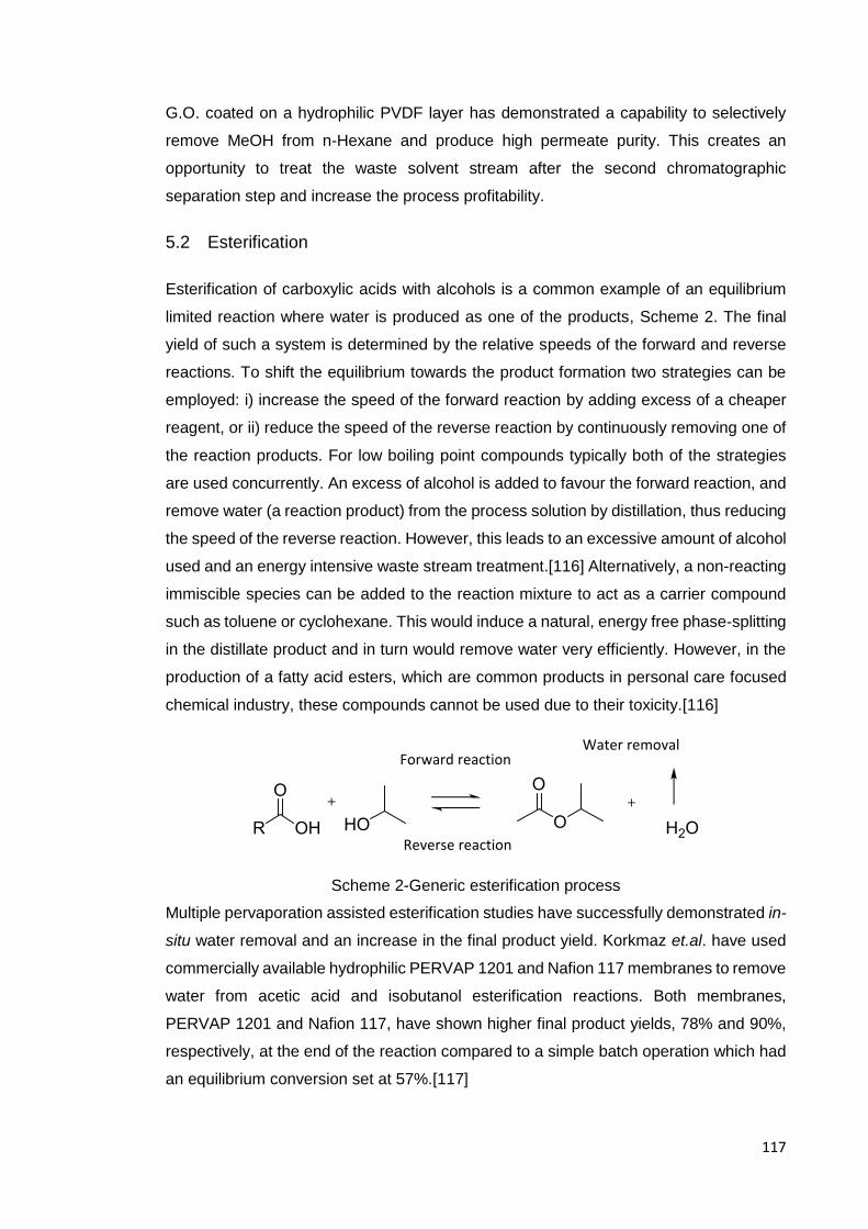
117

G.O. coated on a hydrophilic PVDF layer has demonstrated a capability to selectively

remove MeOH from n-Hexane and produce high permeate purity. This creates an

opportunity to treat the waste solvent stream after the second chromatographic

separation step and increase the process profitability.

5.2 Esterification

Esterification of carboxylic acids with alcohols is a common example of an equilibrium

limited reaction where water is produced as one of the products, Scheme 2. The final

yield of such a system is determined by the relative speeds of the forward and reverse

reactions. To shift the equilibrium towards the product formation two strategies can be

employed: i) increase the speed of the forward reaction by adding excess of a cheaper

reagent, or ii) reduce the speed of the reverse reaction by continuously removing one of

the reaction products. For low boiling point compounds typically both of the strategies

are used concurrently. An excess of alcohol is added to favour the forward reaction, and

remove water (a reaction product) from the process solution by distillation, thus reducing

the speed of the reverse reaction. However, this leads to an excessive amount of alcohol

used and an energy intensive waste stream treatment.[116] Alternatively, a non-reacting

immiscible species can be added to the reaction mixture to act as a carrier compound

such as toluene or cyclohexane. This would induce a natural, energy free phase-splitting

in the distillate product and in turn would remove water very efficiently. However, in the

production of a fatty acid esters, which are common products in personal care focused

chemical industry, these compounds cannot be used due to their toxicity.[116]

Scheme 2-Generic esterification process

Multiple pervaporation assisted esterification studies have successfully demonstrated in-

situ water removal and an increase in the final product yield. Korkmaz et.al. have used

commercially available hydrophilic PERVAP 1201 and Nafion 117 membranes to remove

water from acetic acid and isobutanol esterification reactions. Both membranes,

PERVAP 1201 and Nafion 117, have shown higher final product yields, 78% and 90%,

respectively, at the end of the reaction compared to a simple batch operation which had

an equilibrium conversion set at 57%.[117]

118

Despite the numerous successful pervaporation studies, the use of the membrane

technology where reaction and product removal is combined is limited due to several

drawbacks. A major polymeric membrane shortcoming is their resistance to organic

solvents at elevated temperatures.[29] Inorganic pervaporation membranes cannot

tolerate acidic conditions, for example zeolite membranes immediately denature even at

mild acidic conditions.[45] To circumvent the material degradation by esterification

mixture inorganic membranes can be used in a vapour permeation mode.[116]

To the best of our knowledge, G.O. membranes have not been used before for a

selective water removal from an esterification reaction mixture. It was anticipated that

the G.O. membrane will be able to tolerate acidic conditions without a loss in

performance. The only pervaporation system limitation was imposed by a hydrophilic

PVDF polymeric support, which has limited the range process temperature.

It is important to note that due to the experimental setup, shown in a simplistic view in

Figure 43, the rate of conversion is not comparable with a simple batch operation. The

stock solution was recirculated between the stock solution vessel where it was

maintained at a room temperature, and a pervaporation cell, where the reaction was

taking place.

Pervaporation Cell

StorageVessel

Pump

Vacuum LIne

Figure 43-Pervaporation assisted esterification reaction setup

The esterification reaction was conducted using a pervaporation setup with and without

a G.O. membrane. In the study without the selective water removal the G.O. membrane

was replaced by an impermeable PTFE disk.

The effects of a G.O. membrane on an esterification conversion are shown in Figure 44.

An esterification reaction at 100°C without a selective water removal has reached 58%

conversion after 16 hours. The selective water removal from the reaction mixture has

increased the conversion to 77% within the same time frame. The experiment was then

Reaction Zone

No

reaction

119

repeated without replacing the membrane in the pervaporation cell. Interestingly, the

conversion after 16 hours was only 69%. In both cases, the first run and the repeat, water

removal from the reaction mixture has increased the conversion. A cumulative

permeation flux and the permeate purity time plot are shown in Figure 45. The permeate

purity remained high at 99wt% water value throughout the first 21 hours of

experimentation. This shows that the G.O. membrane was capable of separating water

from the esterification reaction with high selectivity. The value dropped to 85 wt% water

in the permeate in the last two samples. This is most likely a result of a perished rubber

seal between the membrane and the permeation cell, which resulted in a minute leak

and could be avoided by selecting a seal which is more compatible with the reaction

products.

The permeate flux could not be maintained at a stable value, Figure 45. Initially, a high

0.65 kg h-1 m-2 water flux was measured. This was followed by a large decrease to 0.18

kg h-1 m-2 permeation rate, which has linearly declined for the remainder of the

experimental time to 0.043 kg h-1 m-2.

Pervaporation flux change with respect to the theoretical water wt% in the process

solution is shown in Figure 46. There was no obvious correlation between pervaporation

flux and water concentration in the process solution. The highest permeation rate was

observed at 1.6wt% water in the reaction mixture which was the lowest water wt% in the

entire study. An increase in the water concentration in the process solution did not

increase the permeation rate, leading to a conclusion that the permeation flux was

strongly affected by other factors such as membrane degradation at elevated

temperatures.

120

Figure 44-Effects of selective water removal on esterification reaction conversion, 100°C, 2.1μm membrane

Figure 45-Pervaporation flux and permeate purity vs time, 100°C, 2.1μm membrane

0

10

20

30

40

50

60

70

80

90

100

0 2 4 6 8 10 12 14 16 18

Co

nve

rsio

n (

%)

Time (h)

Esterification membrane (1st run) Esterification membrane (2nd run)

Esterification without membrane

0

10

20

30

40

50

60

70

80

90

100

0

0.1

0.2

0.3

0.4

0.5

0.6

0.7

0 5 10 15 20 25 30 35

Time (h)

Per

mea

te W

ater

(w

t%)

Flu

x (k

g h

-1 m

-2)


Run 1 Run 2

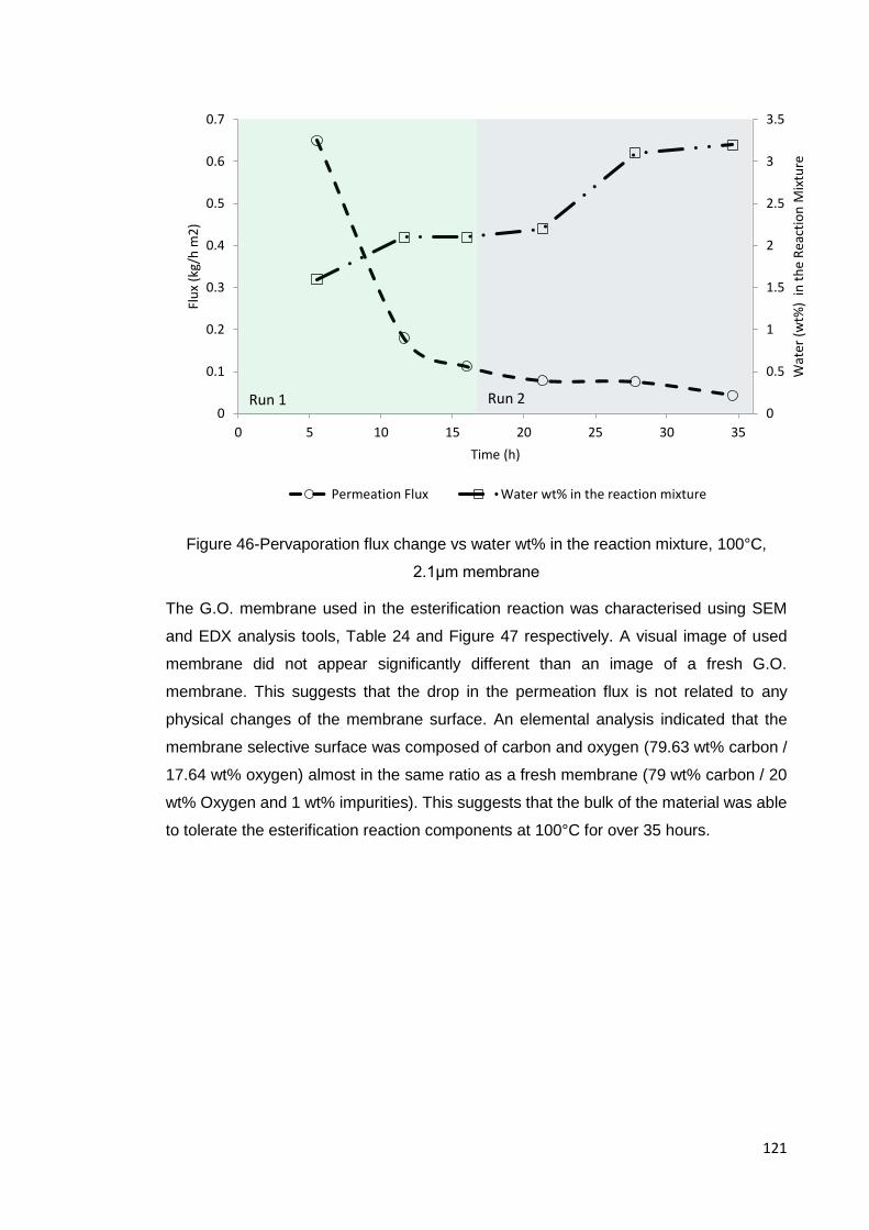
121

Figure 46-Pervaporation flux change vs water wt% in the reaction mixture, 100°C,

2.1μm membrane

The G.O. membrane used in the esterification reaction was characterised using SEM

and EDX analysis tools, Table 24 and Figure 47 respectively. A visual image of used

membrane did not appear significantly different than an image of a fresh G.O.

membrane. This suggests that the drop in the permeation flux is not related to any

physical changes of the membrane surface. An elemental analysis indicated that the

membrane selective surface was composed of carbon and oxygen (79.63 wt% carbon /

17.64 wt% oxygen) almost in the same ratio as a fresh membrane (79 wt% carbon / 20

wt% Oxygen and 1 wt% impurities). This suggests that the bulk of the material was able

to tolerate the esterification reaction components at 100°C for over 35 hours.

0

0.5

1

1.5

2

2.5

3

3.5

0

0.1

0.2

0.3

0.4

0.5

0.6

0.7

0 5 10 15 20 25 30 35

Wat

er (

wt%

) in

th

e R

eact

ion

Mix

ture

Flu

x (k

g/h

m2

)

Time (h)

Permeation Flux Water wt% in the reaction mixture

Run 1 Run 2

122

Table 24-Visual G.O. membrane characterisation

Experiment Conditions and

comments

SEM image

Fatty carboxylic

acid and IPA

esterification at

100°C

Used

membrane, 2 µm

zoom.

N/A Fresh

membrane, 1 µm

zoom.

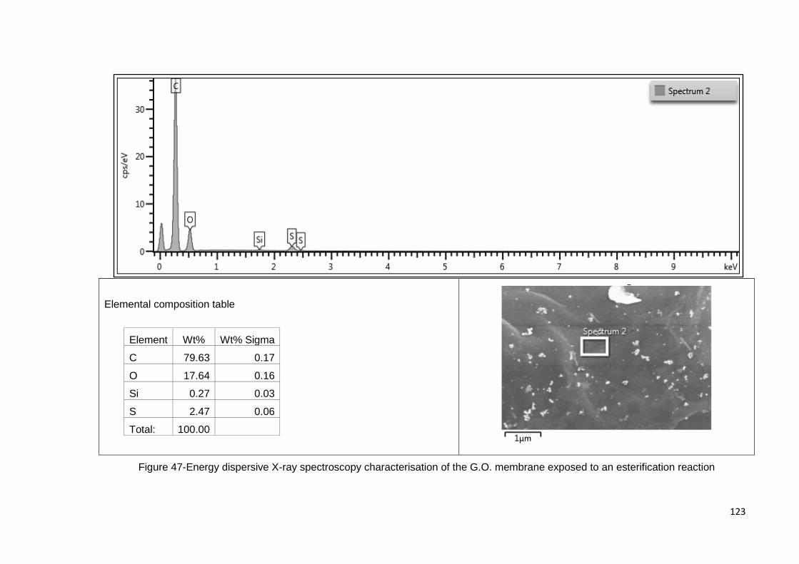
123

Elemental composition table

Element Wt% Wt% Sigma

C 79.63 0.17

O 17.64 0.16

Si 0.27 0.03

S 2.47 0.06

Total: 100.00

Figure 47-Energy dispersive X-ray spectroscopy characterisation of the G.O. membrane exposed to an esterification reaction

124

The change in the G.O. membrane surface chemistry was investigated using FT-IR,

Figure 48. A large double headed peak appeared at 2919 and 2854 cm-1, which was

attributed to an alkane (-CH3 and -CH2-) symmetric and antisymmetric stretching. The

peak may originate from either surface bonded carboxylic acid or IPA. Interestingly,

similar surface chemistry change was observed in the water/IPA dewatering chapter

“Organic Solvent Dehydration”. The fingerprint region had a significantly different

landscape than an unused membrane or G.O. used in the IPA dewatering study. The

emergence of new peaks in the fingerprint region is likely to be a result of the thermal

decomposition of the G.O. at elevated temperatures[103] and permanently bonded

esterification reaction compounds. To date it is not known whether it is possible to avoid

the surface chemical change and retain the permeate flux and the membrane selectivity.

Figure 48-FT-IR spectrum of used (esterification reaction, 100°C, 2.1μm membrane) and fresh G.O. membrane

5001000150020002500300035004000

No

rmal

ised

ab

sorp

tio

n (

A.U

.)

Wavelength (cm-1)

Fresh Membrane Used Membrane

125

To complement the FT-IR study, water contact angle measurements were made, Figure

49. A water drop contact angles has significantly increased from approximately 66° (fresh

G.O. membrane) to 83° (used G.O. membrane). The increased contact angle shows a

decrease in the material hydrophilicity which is known to negatively impact the water

permeation flux and membrane selectivity.[118] The issue could be addressed by

modifying the material surface chemistry and attaching more stable functional groups.

Figure 49 - Water contact angle on the a) fresh G.O. membrane, and b) used G.O.

membrane in an esterification reaction

b) a )

66.0° 65.2° 83.0° 83.5°

126

5.3 Peptides

A membrane separation process is an attractive water removal technique, not only for

challenging azeotropic mixtures, but also for highly aqueous protein solutions. Large

scale dewatering is typically conducted via distillation. However, large molecular species

such as peptides or proteins can degrade at high temperatures. This severely limits the

rate of water removal in a distillation process and makes equipment underutilised. A

membrane process can remove large quantities of water under mild conditions and a

relatively small floor footprint due to its compact module design.[85]

An incorporation of a G.O. sheets into a polymeric membrane matrix has previously

shown a good water separation rate and a decreased membrane surface fouling[119],

which is especially prominent in a peptide separation processes.[120] In this case study,

2.1 µm G.O. membranes were used in a water removal operation from highly aqueous

peptide solutions.

The current peptide dewatering process uses vacuum distillation to evaporate

approximately 10,000 kg water at 80°C. One operation takes 6-10 h, which translates to

the following rate of water removal 1000-1666 kg/h. The variation in the rate of water

removal is attributed to the following two factors: i) initial solids content, and ii) a variation

in the steam temperature.

To improve industrial peptide dewatering process several key factors were identified:

i) Processing time reduction

ii) Lower processing temperature

iii) Improved quality of the product

Initial DI (deionised) water pervaporation tests at a 70°C and 90°C resulted in a 5.43 and

9.8 kg h-1 m-2 flux respectively. Pervaporation flux at 80°C was estimated using prior data

to be approximately 8 kg h-1 m2. This approximation allows for a facile required

membrane surface area calculation to remove 10000 kg in 6-10 h, Table 25.

Table 25-Estimates of membrane areas required to replace current evaporator process

Operation Time (h) Area (m2) at 70°C Area (m2) at 80°C

6 307 208

10 184 125

5.3.1 Peptide 1 Hydrolysate

Pervaporation of an aqueous Peptide 1 hydrolysate solution was conducted at 80°C and

2-8wt% solids in water content over a course of several days, resulting in a total

experiment time of ≈34 h. The purpose of this study was to investigate the pervaporation

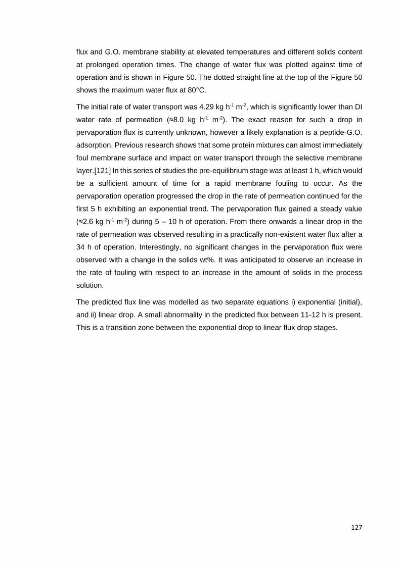
127

flux and G.O. membrane stability at elevated temperatures and different solids content

at prolonged operation times. The change of water flux was plotted against time of

operation and is shown in Figure 50. The dotted straight line at the top of the Figure 50

shows the maximum water flux at 80°C.

The initial rate of water transport was 4.29 kg h-1 m-2, which is significantly lower than DI

water rate of permeation (≈8.0 kg h-1 m-2). The exact reason for such a drop in

pervaporation flux is currently unknown, however a likely explanation is a peptide-G.O.

adsorption. Previous research shows that some protein mixtures can almost immediately

foul membrane surface and impact on water transport through the selective membrane

layer.[121] In this series of studies the pre-equilibrium stage was at least 1 h, which would

be a sufficient amount of time for a rapid membrane fouling to occur. As the

pervaporation operation progressed the drop in the rate of permeation continued for the

first 5 h exhibiting an exponential trend. The pervaporation flux gained a steady value

(≈2.6 kg h-1 m-2) during 5 – 10 h of operation. From there onwards a linear drop in the

rate of permeation was observed resulting in a practically non-existent water flux after a

34 h of operation. Interestingly, no significant changes in the pervaporation flux were

observed with a change in the solids wt%. It was anticipated to observe an increase in

the rate of fouling with respect to an increase in the amount of solids in the process

solution.

The predicted flux line was modelled as two separate equations i) exponential (initial),

and ii) linear drop. A small abnormality in the predicted flux between 11-12 h is present.

This is a transition zone between the exponential drop to linear flux drop stages.

128

Figure 50-Pervaporation of aqueous Peptide 1 Hydrolysate (2 – 8wt% solids) at 80°C, 2.1 µm membrane

For an extremely dilute system containing only 2wt% solids it was anticipated to achieve

DI water rate of permeation. It is important to note that the model fitted flux at 0 h does

not match pure water pervaporation rate. This may be a result of i) inaccurate

interpolation of DI water data, or ii) immediate interaction between peptides and G.O.

surface. It is also important to note that the initial pervaporation data is lost due to pre-

equilibration stage, which was ≥ 1 h.

Two new sets of required surface areas were estimated at initial flux and a semi steady-

state flux as 233 – 389 m2 and 385 – 641 m2 respectively.


The Peptide 2 peptide solution dewatering was conducted at 80°C over a period of 26 h.

The rate of water permeation was plotted against time of operation and is shown in Figure

51. The dotted straight line (8 kg h-1 m-2) shows the maximum rate of permeation at 80°C

interpolated from previous DI water permeation data. The initial rate of permeation was

found to be 5.2 kg h-1 m-2. At a similar time of operation Peptide 1 peptide had almost 1

kg h-1 m-2 lower flux than Peptide 2 peptide solution. It is not known whether this is a

result of different pH or structure/molecular weight of the peptides present in the solution.

The semi steady-state rate of permeation at 3.6 kg h-1 m-2 was reached after 2 hours of

0

1

2

3

4

5

6

7

8

9

0 5 10 15 20 25 30 35

Flu

x (k

g h

-1m

-2)

Time (h)

Experimental Predicted DI Water

4.29 kg h-1 m-2, 233 – 389 m2

2.6 kg h-1 m-2, 385 – 641 m2

2wt% solids in water



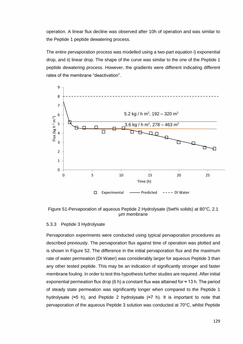
129

operation. A linear flux decline was observed after 10h of operation and was similar to

the Peptide 1 peptide dewatering process.

The entire pervaporation process was modelled using a two-part equation i) exponential

drop, and ii) linear drop. The shape of the curve was similar to the one of the Peptide 1

peptide dewatering process. However, the gradients were different indicating different

rates of the membrane “deactivation”.

Figure 51-Pervaporation of aqueous Peptide 2 Hydrolysate (5wt% solids) at 80°C, 2.1 µm membrane


Pervaporation experiments were conducted using typical pervaporation procedures as

described previously. The pervaporation flux against time of operation was plotted and

is shown in Figure 52. The difference in the initial pervaporation flux and the maximum

rate of water permeation (DI Water) was considerably larger for aqueous Peptide 3 than

any other tested peptide. This may be an indication of significantly stronger and faster

membrane fouling. In order to test this hypothesis further studies are required. After initial

exponential permeation flux drop (6 h) a constant flux was attained for ≈ 13 h. The period

of steady state permeation was significantly longer when compared to the Peptide 1

hydrolysate (≈5 h), and Peptide 2 hydrolysate (≈7 h). It is important to note that

pervaporation of the aqueous Peptide 3 solution was conducted at 70°C, whilst Peptide

0

1

2

3

4

5

6

7

8

9

0 5 10 15 20 25

Flu

x (k

g h

-1m

-2)

TIme (h)

Experimental Predicted DI Water

3.6 kg / h m2, 278 – 463 m2

5.2 kg / h m2, 192 – 320 m2

130

1 and Peptide 2 hydrolysates were dewatered at 80°C. It is known that the process

temperature affects the membrane fouling rate.[121]

Figure 52-Pervaporation of aqueous Peptide 3 (2wt% solids) solution at 70°C, 2.1 µm

membrane

0

1

2

3

4

5

6

0 2 4 6 8 10 12 14 16 18 20

Flu

x (k

g h

-1m

-2)

Time (h)

Pervaporation Flux Predicted DI Water

1.1 kg h-1m-2 909 – 1515m2

0.52 kg h-1m-2 1923 – 3205m2

131

Membranes from the i) Peptide 1, ii) Peptide 2 and iii) Peptide 3 dewatering experiments

were analysed using SEM and EDX. To draw an objective comparison between used

and fresh membrane surface morphologies an unused membrane image is shown in

Table 26. The unused membrane SEM image had a typical surface structure of a G.O.

membrane and was a match to the previous research data.[109]

Table 26-Unused G.O. membrane SEM images

Experiment Conditions

and

comments

SEM image

N/A Fresh

membrane,

10 µm zoom.

N/A Fresh

membrane, 1

µm zoom.

132

SEM images of the membranes used in the peptide dewatering processes and are

shown in Figure 53. All three membranes exhibited different surface morphologies

compared to an unused membrane shown in Table 26. The characteristic coarse

structure G.O. surface has completely disappeared. Surfaces of the membranes used in

dewatering Peptide 1 and Peptide 3 peptides were relatively smooth at a 100 µm scale.

The membrane used in the Peptide 2 dewatering process did not share the same surface

morphology at a 100 µm scale.

Upon a closer investigation,2 µm zoom, membrane exposed to the Peptide 1 peptide still

had a relatively smooth surface and was clearly fouled with the peptide. Membranes

exposed to Peptide 3 and Peptide 2 peptides at 2 µm scale had similar surface

appearance. The highlighted regions were attributed to a peptide presence at the

periphery of the G.O. sheets, which could result from a physisorption or chemisorption

process between the G.O. sheet and a peptide functional groups. Interestingly, in the

image of the membrane exposed to the Peptide 2 peptide a subsurface of the G.O.

membrane can be seen. This would imply that the peptide has bonded to several layers

of the G.O. membrane. Physically hindered access between the membrane sheets would

inhibit water intercalation into the membrane matrix and negatively impact on the rate of

water permeation.

EDX spectroscopy was performed on all of the membranes. The analysis showed a

presence of various elements on the surface of the membranes confirming the presence

of the peptides. Initially, it was thought that the graphene oxide was chemically altered

at elevated temperatures, which has been observed to occur in an alkaline and highly

acidic media,[115, 122] and could lead to a drop in a pervaporation flux. In case of the

chemical reduction a high increase in the carbon/oxygen ratio was anticipated from an

initial 4/1 to 12/1.[115] All of the membranes have retained high oxygen content ranging

from C/O 3.42, Figure 56, to 4.58, Figure 54. A high amount, 7.67 wt%, of chloride was

found on the surface of a membrane exposed to the Peptide 3 peptide. A minute amounts

of chloride (0.22) was also found on the membrane surface used in the Peptide 2 peptide

dewatering process. Previous research has highlighted that chloride can permanently

bond to the surface via SN2 reaction mechanism.[115] Due to peak overlap it was not

possible to tabulate accurate amounts of nitrogen present on the membrane surface.

Only a small area scan, Figure 56, showed a significant amount of nitrogen, 9.11 wt%,

present on the surface; a key element in all of the peptides.

133

Figure 53-SEM images of membranes used in i) Peptide 1 hydrolysate, ii) Peptide 3, and iii) Peptide 2 peptide dewatering processes

Peptide 1 (700 Da), pH = 4 Peptide 3 (1200 Da), pH =5.5 Peptide 2 (2000 Da), pH = 9.9

100 µm zoom 100 µm zoom 100 µm zoom

2 µm zoom 2 µm zoom 2 µm zoom

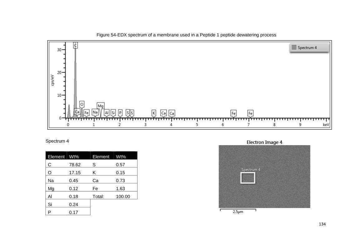
134


Spectrum 4

Element Wt% Element Wt%

C 78.62 S 0.57

O 17.15 K 0.15

Na 0.45 Ca 0.73

Mg 0.12 Fe 1.63

Al 0.18 Total: 100.00

Si 0.24

P 0.17

135


Spectrum 5


C 67.19 Cl 7.67

O 17.26 Ca 2.53

Na 0.36 Total: 100.00

Mg 0.12

Al 0.15

Si 4.42

S 0.29

136

Figure 56-EDX spectrum of a membrane used in a Peptide 2 peptide dewatering process (scan1)

Spectrum 6


C 62.29 S 0.75

N 9.11 Cl 0.22

O 18.22 Ca 3.72

Na 3.81 Total: 100.00

Mg 0.90

Al 0.39

Si 0.22

P 0.37

137

To complement SEM visual analysis and EDX, surface hydrophilicity was tested by

measuring water droplet contact angle. Images of the water contact angles are shown in

Figure 57. Membranes exposed to the peptide dewatering process exhibited larger contact

angles leading to a reduced membrane surface hydrophilicity. It is not known whether the

change in the contact angle was a result of adhered peptides to the surface or there has

been G.O. membrane degradation.

All three peptides demonstrated very similar rate of permeation trend lines. The process was

separated into three segments: i) high initial flux and exponential decay, ii) constant rate of

permeation, and iii) linear drop in the rate of pervaporation. SEM and EDX analysis

confirmed peptide presence on the surface of the membrane, however, it is not clear whether

there was any preferential fouling by any certain fraction of the peptides in the solution.

Furthermore, the surface water contact angle has changed and the membranes became

less hydrophilic after exposure to an alkaline and acidic aqueous peptide solutions.

Currently, it is not clear if it is possible to regenerate the membrane surface or has it been

permanently altered.

Peptides and proteins are known to accumulate on a surface of a membrane and produce

a fouling layer over time. It is difficult to determine whether there is a specific set of

compounds responsible for the loss of the rate of water permeation. An in depth review has

been previously published covering various aspects contributing to the surface fouling and

analysis methods used to investigate cake layer.[120] In this instance, more experimentation

is required to determine the exact nature of the membrane deactivation.

Figure 57 – Water contact angles of a) Unused membrane, b) Peptide 3 peptide exposed membrane, and c) Peptide 2 peptide exposed membrane

a) b) c)

138

6 Process Modelling and Economics

The purpose of this chapter is to evaluate the economic benefits of a pervaporation process

using G.O. membranes. Dewatering of an aqueous IPA solution was selected as a case

study. Membrane process, modelled by an in-house developed code and Aspen Plus, is

compared to an azeotropic distillation, modelled by Aspen Plus, in terms of their energy

consumption. Furthermore, G.O. membrane capability to dehydrate aqueous IPA solution

to a various degrees of water content are discussed. The design specifications of the

selected case study are summarised in Table 27.

Table 27-Selected case study design specifications

Components Flow (kg h-1) Temperature

(°C)

Pressure

(bar)

Product Purity

(wt%)

Recovery

(%)

IPA 700 25 1.01 95 99

Water 300 25 1.01 >99 ≅87.8

IPA is a bulk chemical used in many different industries with the total annual production of

550,000 tons in 1992 in Europe.[123] It is mainly encountered as a solvent in paint and

plastic manufacturing.[123] The compound can also be used as a reactant in the production

of mono-isopropyl amine and isopropyl acetate.[124] Frequently, the IPA waste stream

contains water and it is desired to recycle the organic solvent. [123] A water rich IPA waste

stream forms a minimum boiling point (80.4°C) azeotropic mixture (87.7 wt%, IPA, 1.01 bar),

Figure 58. As mentioned before, this mixture cannot be separated by a conventional

distillation and an azeotropic distillation has to be used. The process is typically very energy

intensive and expensive to run.[8]Pervaporation is seen as an energy saving alternative and

is frequently implemented on a large scale.[123]

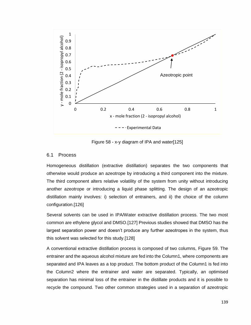
139

Figure 58 - x-y diagram of IPA and water[125]

6.1 Process

Homogeneous distillation (extractive distillation) separates the two components that

otherwise would produce an azeotrope by introducing a third component into the mixture.

The third component alters relative volatility of the system from unity without introducing

another azeotrope or introducing a liquid phase splitting. The design of an azeotropic

distillation mainly involves: i) selection of entrainers, and ii) the choice of the column

configuration.[126]

Several solvents can be used in IPA/Water extractive distillation process. The two most

common are ethylene glycol and DMSO.[127] Previous studies showed that DMSO has the

largest separation power and doesn’t produce any further azeotropes in the system, thus

this solvent was selected for this study.[128]

A conventional extractive distillation process is composed of two columns, Figure 59. The

entrainer and the aqueous alcohol mixture are fed into the Column1, where components are

separated and IPA leaves as a top product. The bottom product of the Column1 is fed into

the Column2 where the entrainer and water are separated. Typically, an optimised

separation has minimal loss of the entrainer in the distillate products and it is possible to

recycle the compound. Two other common strategies used in a separation of azeotropic

0

0.1

0.2

0.3

0.4

0.5

0.6

0.7

0.8

0.9

1

0 0.2 0.4 0.6 0.8 1

y -

mo

le f

ract

ion

(2

-is

op

rop

yl a

lco

ho

l)

x - mole fraction (2 - isopropyl alcohol)

Experimental Data

Azeotropic point

140

mixtures are: pressure swing distillation or heterogeneous azeotropic distillation. Some

mixtures shift their azeotropic point when the pressure is changed, this can be used to

separate the mixtures into its constituents. Heterogeneous azeotropic distillation introduces

a third component which is not miscible with the mixture. This results in a natural phase split

and removal of relatively high purity products.[123, 127, 129, 130]

Column1 Column2

Water

Condenser1 Condenser2

IPA/Water

Reboiler2Reboiler1

Entrainer

Entrainer Recycle

IPA

Figure 59-Conventional extractive distillation

6.2 Simulation method

Aspen Plus has 4 simulation methodologies for solving separation problems. The choice of

the correct model is dictated by the complexity of the process. One of the common models

is “SEP2”, which is a general-purpose unit operation. It does not include the number of trays

or a reflux ratio, therefore it is used just as a general screening tool. Another general

distillation model is DSTWU. It uses Gilliland’s (required reflux ratio for a specified number

of stages), Winn’s (minimum number of stages) and Underwood’s (minimum reflux ratio)

methods to calculate the number of stages and reflux ratios. Named shortcuts assume: i)

constant molar overflow, and ii) constant relative volatility. However, due to the complexity

of the extractive distillation, shortcut methods cannot be used to simulate the process.[131]

141

In this work a more rigorous model, RadFrac, is used, which can simulate a number of trays,

random packing and structured packing in the column. This model is applicable to: i)

conventional distillation, ii) absorption, and ii) extractive or azeotropic distillation. In this work

it was assumed that equilibrium is reached at each stage, thus columns were set in

equilibrium mode. Alternatively, Murphree or vaporisation efficiencies can be specified to

solve this distillation problem.

The RadFrac model solves a number of simultaneous equations: phase equilibrium

(Equation 75), component mass balance (Equation 76), total mass balance (Equation 77),

and enthalpy balance (Equation 78). The mass flow balance is shown graphically in Figure

60. Initially the model either guesses temperature, pressure, liquid and vapour compositions

and their corresponding flow rates or uses user provided values.

𝑦𝑖,𝑛 − 𝑘𝑖,𝑛 𝑋𝑖,𝑛 = 0 Equation 75

−𝑙𝑖,𝑛−1 + 𝑙𝑖,𝑛 + 𝑣𝑖,𝑛 − 𝑣𝑖,𝑛+1 − 𝑓𝑖,𝑛 = 0 Equation 76

−𝐿 𝑛−1 + 𝐿 𝑛 + 𝑉𝑛 − 𝑉𝑛+1 − 𝐹𝑛 = 0 Equation 77

−𝐻 𝑛−1 𝐿 𝐿 𝑛−1 + 𝐻 𝑛

𝐿 𝐿 𝑛 + 𝐻 𝑛𝑉 𝑉 𝑛 − 𝐻 𝑛+1

𝑉 𝑉𝑛+1 − 𝐹 𝑛𝐻 𝑛𝐹 − 𝑄𝑛 = 0 Equation 78

Stage, n

Mass Flow Balance

Fn

(feed) Qn

(heat added)

Ln-1

(liquid leaving stage n)

Ln

(liquid entering stage n)

Vn

(vapour entering stage n)

Vn+1

(vapour leaving stage n)

Figure 60 – Mass flow balance on a single stage

142

A Non-ideal algorithm was used to converge RadFrac column with a standard initialization

technique, which is tailored to model a non-ideal mixture. The vapour phase was modelled

as an ideal gas while a non-ideal liquid phase activity coefficient was calculated using the

NRTL model. The NRTL model and parameters are shown in Equation 79, Equation 80 and

Table 28.

Table 28-NRTL Parameters from Aspen Plus Properties Database

Parameter Binary Pair

Component i WATER WATER IPA

Component j IPA DMSO DMSO

AIJ 6.8284 -1.2449 0

AJI -1.3115 1.7524 0

BIJ -1483.4573 586.801 115.2787

BJI 426.3978 -1130.2155 -25.0123

CIJ 0.3 0.3 0.3

ln(𝛾𝑖) =∑ 𝑥𝑗𝜏𝑗𝑖𝐺𝑗𝑖𝑗

∑ 𝑥𝑘𝐺𝑘𝑖𝑘+ ∑

𝑥𝑗𝐺𝑖𝑗

∑ 𝑥𝑘𝐺𝑘𝑗𝑘(𝜏𝑖𝑗 −

∑ 𝑥𝑚𝜏𝑚𝐺𝑚𝑗𝑚

∑ 𝑥𝑘𝐺𝑘𝑗𝑘)

𝑗

Equation 79

Where

𝐺𝑖𝑗 = exp(−𝛼𝑖𝑗𝜏𝑖𝑗) , 𝜏𝑖𝑗 = 𝛼𝑖𝑗 +𝑏𝑖𝑗

𝑇, 𝛼𝑖𝑗 = 𝑐𝑖𝑗, 𝜏𝑖𝑖 = 0, 𝐺𝑖𝑖 = 1

Equation 80

143

A homogeneous extractive distillation of Water/IPA solution using DMSO as an entrainer

was optimised for the re-boiler duty by varying the following parameters: i) DMSO flow rate,

ii) total number of stages iii) feed stage of IPA/Water, and iv) feed stage of DMSO. Optimal

conditions were found using typical optimisation strategy [127]:

1. Guess initial DMSO feed flow rate

2. Guess a total number of plates

3. Guess fresh feed and DMSO feed stages in the column (DMSO below the IPA/Water

feed)

4. Set the distillate flow rate (based on the process specifications)

5. Change DMSO flow rate and re-boiler duty until design specifications are met

6. Lower feed stages to a minimum

7. Change DMSO and IPA/Water feed stages

8. Repeat step 5

The extractive distillation process has two columns, which makes it computationally

intensive to optimise all variables at the same time. Thus an extractive column was optimised

first, because it was more important to reach the desired dewatered alcohol purity than the

quality of the water waste stream.

6.3 Energy Consumption Modelling-Distillation

An optimised azeotropic distillation process is shown in Figure 61. The first column was

composed of 20 theoretical stages (including condenser and re-boiler). Preheated

Water/IPA solution was fed into the extractive column above stage 16 and the entrainer was

fed above stage 3. The column section between the Water/IPA feed and the entrainer feed

is called an extraction zone. The purpose of this section is to strip out water by lowering the

relative volatility of the water using DMSO. The water then leaves the column as a bottom

product. The top part of the column (above DMSO feed) contains mainly IPA and a minute

amount of water. This component mixture does not form an azeotrope, thus the light

component (IPA) is separated from the high boiling point DMSO and leaves as a top product.

The optimised entrainer recovery column was composed of 10 theoretical stages (including

re-boiler and condenser). The distillate product was almost pure (99.99wt%) water and a

small amount of DMSO (0.01 wt%); the bottom product of the column high purity DMSO,

which was suitable for a recycle

144

Figure 61-Extractive distillation of the IPA

COL2COL1

HE2

HE1

BOTTPRO1

DIST02

BOTTPRO2

FEEDIN2

DMSOIN2

DIST01

FEEDIN1

HWIN2

HWOUT2

DMSOIN1

BPRD2OUT

1000 kg/h

300 kg/h H2O (30 wt%)

700 kg/h IPA (70 wt%)

289.22 kg/h

DMSO (100 wt%)

Duty: 48.82 kW

Duty: 340.00 kW Duty: 218.81 kW

NT=20

NFEEDin2

=3

NDMSOIN2

=16

Duty: 239.743 kW Duty: 239.74 kW

736.72 kg/h

36.7 kg/h H2O (5.0 wt%)

700 kg/h IPA (95.0 wt%) 0.017 kg/h DMSO (minute)

263.32 kg/h 263.3 H

2O (99.99 wt%)

0.02 kg/h DMSO (0.01 wt%)

289.21 kg/h

DMSO (99.99 wt%)

NT=10

NBOTTPRO1

=7

T=190.7 °C

T=100.0 °C

T=108.4 °C

T=70 °C

T=70 °C

T=25 °C

T=25 °C

T=152 °C

T=80.7 °C

145

Liquid composition profiles of the extractive column are shown in Figure 62. The goal of the

DMSO (change relative volatility in the extractive column) was achieved and the majority of

the water was retained in the extraction section. The distillate product was composed of

95wt% IPA and 5wt% water with minute amounts of DMSO; this was deemed to be

acceptable. The stripping section, between the plates 16 and 20, had a rapidly diminishing

amount of IPA. As the lightest component IPA evaporated and was returned to the extractive

part of the column. The bottom product was composed of 52.34wt% DMSO and 47.65wt%

water. The amount of IPA leaving as a bottom product was negligible, thus the overall

recovery of the compound was greater than 99.99 wt%.

Figure 62 - Composition profiles in the extractive column

The purpose of the second column was to recover the entrainer (DMSO) and produce high

purity water as the distillate. The composition profile of the recovery column is shown in

Figure 63. Very high purity water, 99.99wt%, was obtained as a distillate and only 0.006 wt%

DMSO was lost through the top product of the recovery column. The bottom product of the

recovery column resulted in a high 99.99wt% DMSO purity. The recovered entrainer can

then be reused as a feed stream to the extractive column (not shown in Figure 61).

0

0.1

0.2

0.3

0.4

0.5

0.6

0.7

0.8

0.9

1

1 2 3 4 5 6 7 8 9 10 11 12 13 14 15 16 17 18 19 20

Liq

uid

Mas

s Fr

acti

on

Stage (condenser = 1, reboiler = 20)

IPA Water DMSO

Bottom

Section

Extractive Section

Top S

ection

DMSO Feed

Water/IPA Feed

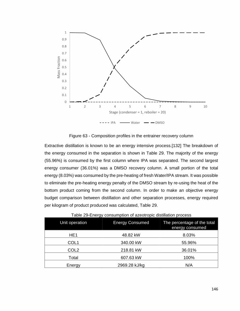
146

Figure 63 - Composition profiles in the entrainer recovery column

Extractive distillation is known to be an energy intensive process.[132] The breakdown of

the energy consumed in the separation is shown in Table 29. The majority of the energy

(55.96%) is consumed by the first column where IPA was separated. The second largest

energy consumer (36.01%) was a DMSO recovery column. A small portion of the total

energy (8.03%) was consumed by the pre-heating of fresh Water/IPA stream. It was possible

to eliminate the pre-heating energy penalty of the DMSO stream by re-using the heat of the

bottom product coming from the second column. In order to make an objective energy

budget comparison between distillation and other separation processes, energy required

per kilogram of product produced was calculated, Table 29.

Table 29-Energy consumption of azeotropic distillation process

Unit operation Energy Consumed The percentage of the total energy consumed

HE1 48.82 kW 8.03%

COL1 340.00 kW 55.96%

COL2 218.81 kW 36.01%

Total 607.63 kW 100%

Energy 2969.28 kJ/kg N/A

0

0.1

0.2

0.3

0.4

0.5

0.6

0.7

0.8

0.9

1

1 2 3 4 5 6 7 8 9 10

Mas

s Fr

acti

on

Stage (condenser = 1, reboiler = 20)

IPA Water DMSO

147

7 Pervaporation separation of Water/IPA mixtures

7.1 Process

Membrane process modelling can be split into three distinct parts which serve different

purposes: i) membrane scale-parameter estimation, ii) unit scale-mass and heat transfer in

the module assessment, and iii) large scale-process economics study of the whole

operation.[8, 133, 134]

Membrane scale modelling has a rich history and many different theories have been

proposed over time. An in-depth review of multiple available models has been published

recently.[135] The difficulty in applying these models arise from the lack of their applicability

for different solute, solvent and membrane material systems. Recently, seven different

membrane separation models have been compared with each other in terms of their fit to

the experimental data. It was shown that solution-diffusion based models gave a better fit to

a permeation data collected from a flexible-chain glassy membranes whereas the pore-flow

model gave a better fit to the data obtained from a glassy membranes with a rigid structure.

[136] A simulation of a membrane separation process requires the selection of an

appropriate permeation model and some experimental effort to support the model selection.

At a modular scale it is assumed that the correct model for the permeation has been

selected. The simulation focus shifts towards the fluid dynamics and mass transfer

properties in the membrane module.[136] On this scale, the concentration polarisation and

temperature gradients become important, and If not appropriately addressed, the

performance of the process can be significantly impeded.

To address the issue of the concentration polarisation several experimental strategies have

been developed.[85] One of the methods makes use of the concentration polarisation

expression, Equation 81. The model relies on a correlation between the liquid boundary

layer thickness and process fluid velocity, Equation 82.

ln (1 −1

𝐸) = ln (1 −

1

𝐸0) −

𝐽𝑣𝑦𝑙

𝐷𝑤

Equation 81

𝐷𝑤

𝑦𝑙= 𝐾𝑢𝑛

Equation 82

The model parameters are determined by a linear regression of Equation 81, which gives

an intrinsic enrichment factor, E0, as a function of the fluid velocity.[85] Thereafter, the ratio

148

of the E/E0 is calculated, which gives the magnitude of the concentration polarisation in the

membrane equipment.

Heat transfer effects are typically accounted by considering dimensionless group

correlations and heat balance equations.[94] These concepts link fluid velocity and

temperature to the permeation flux profile in the membrane module.

Liquid mass transfer coefficient is typically determined by varying liquid flowrate on the

process side followed by a parameter fitting to a pervaporation equation. This method is

commonly used among membrane researchers.[94] Another option, is to apply

dimensionless mass transfer coefficient correlations however, this works only when mass

transfer correlations for a given membrane configuration are available.[137] Alternatively,

mass transfer coefficients can be studied by varying the membrane thickness while the

process liquid flowrate is kept constant. This methodology allows separating the liquid and

membrane mass transfer coefficients. It has to be noted that in order for this method to work

membrane has to present a significant part of the overall resistance.[83]

If membrane material is close to commercialisation at this scale the type of the membrane

module should be selected. There are several different options to choose from: spiral wound,

plate and frame, and tubular. The design of the membrane module is mainly determined by

several factors such as: i) cost of the process, ii) fouling control, ii) pressure drop, iii) the

desired operation pressure, and iv) material compatibility.[11]

Large-scale modelling is focused on the capital and operating costs of the pervaporation

alone or in a combination with other chemical engineering processes. Lipnizki has produced

a review article covering a large number of pervaporation case studies.[134] Typically, the

results of large scale pervaporation modelling show significantly reduced operating costs

and smaller capital investment.[8, 134]

7.2 Simulation methodology and process energy requirement

There is no “ready to use” pervaporation model in the Aspen Plus simulation package. To

circumvent this issue and calculate pervaporation energy consumption a model separation

was set-up, Figure 64. The model was split into three parts: i) pre-heating of the process

fluid, ii) separation of the components, and iii) evaporation of the water rich stream

(permeate). A heat exchanger (HE1) was used to pre-heat the process stream from 25°C to

the pervaporation temperature (70°C) which was then fed into the separator (SEP).

Separation in this unit is based on user defined split values for each component, coupled to

149

a rigorous flash calculation to determine the energy required for the separation. It is usually

used as a simplified representation of a distillation process when separation is achieved or

the column is known but the details of the process are not important. In this block, the top

product was set to match the design specifications and leave the process in the liquid phase,

while the bottom product (water rich stream) was flashed into vapour, imitating the phase

change in a pervaporation process.

Overall energy requirements were calculated using Equation 83.

𝐸𝑝𝑟𝑒−ℎ𝑒𝑎𝑡 + 𝐸𝑝ℎ𝑎𝑠𝑒 𝑐ℎ𝑎𝑛𝑔𝑒 + 𝐸𝑣𝑎𝑐𝑢𝑢𝑚 𝑝𝑢𝑚𝑝 = 𝐸𝑡𝑜𝑡𝑎𝑙 Equation 83

Where Epre-heat is energy of the pre-heater (kW), Ephase change, the energy associated with the

phase change of the permeate (kW), Evacuum pump is energy calculation required to run vacuum

pump. The pre-heater and the phase change energy requirements were estimated by Aspen

Plus. The vacuum pump electric power was calculated using Equation 84.[138]

𝐸𝑣𝑎𝑐𝑢𝑢𝑚 𝑝𝑢𝑚𝑝 = 𝑛𝑝𝑒𝑟𝑚𝑒𝑎𝑡𝑒𝑅𝑇𝑝𝑒𝑟𝑚

1

𝜂𝑣𝑎𝑐

𝛾𝑔𝑎𝑠

𝛾𝑔𝑎𝑠 − 1((

𝑃𝑎𝑡𝑚𝑜𝑝ℎ𝑒𝑟𝑖𝑐

𝑃𝑝𝑒𝑟𝑚𝑒𝑎𝑡𝑒)

𝛾𝑔𝑎𝑠−1

𝛾𝑔𝑎𝑠

− 1)

Equation 84

Where Evacuum pump is electric energy required to run the vacuum pump (W), npermeate is a molar

flow of permeate (mol s-1), R is the ideal gas constant (J mol-1 K-1), T is permeate temperature

(K), 𝜂 is the vacuum pump efficiency, γgas is an adiabatic expansion coefficient, Patmospheric is

atmospheric pressure (bar), and Ppermeate is the permeate side pressure, which was set at 30

mbar. The vacuum pump efficiency was calculated using Equation 85.[139]

𝜂 = 0.1058 ln (𝑃𝑝𝑒𝑟𝑚𝑒𝑎𝑡𝑒

𝑃𝑝𝑟𝑜𝑐𝑒𝑠𝑠) + 0.8746

Equation 85

Where Pprocess is water vapour pressure on the process side (bar). The electric power was

then converted to thermal energy using the following conversion 1 kW electric = 2 kW

thermal.

Energy savings provided by the membrane separation were calculated using Equation 86

100 − 𝐸𝑛𝑒𝑟𝑔𝑦(𝑃𝑒𝑟𝑣𝑎𝑝𝑜𝑟𝑎𝑡𝑖𝑜𝑛)

𝐸𝑛𝑒𝑟𝑔𝑦(𝐷𝑖𝑠𝑡𝑖𝑙𝑙𝑎𝑡𝑖𝑜𝑛)∗ 100

Equation 86

150

HE1

SEP

FEED1

IPA

WATER

FEED2

HIN

HOUT

Hot Water Inlet

1000 kg/h

300 kg/h H2O (30 wt%)

700 kg/h IPA (70 wt%)

Hot Water Outlet

736.7 kg/h (Liquid) 36.7 kg/h H

2O (5 wt%)

700 kg/h IPA (95 wt%)

263.3 kg/h (Vapour) 263.3 kg/h H

2O (100.00 wt%)

Duty: 25.5 kW Duty: 178.35 kW

Total Duty: 175.49 kW Energy of Permeation = 862.41 kJ/kg

Figure 64 – Pervaporation energy requirement simulation

T = 25 °C

T = 70 °C

T = 70 °C

T = 70 °C

151

The overall energy requirements of the pervaporation process are shown in Table 30. The

energy required for the evaporation of the permeate stream has dwarfed the pre-heater

energy requirements. Interestingly, the heat required (thermal equivalent) to maintain

vacuum (30 mbar) on the permeate side was almost as high as the energy required for the

evaporation. This makes maintaining vacuum an important consideration when designing

pervaporation process and a trade-off between the vacuum pump operating cost and the

reduced permeation flux should be carefully assessed. A similar energy penalty in a

pervaporation research was found previously while studying acetic acid dewatering process.

[8]

Table 30-Energy consumption of a membrane separation process

Unit operation Energy Consumed (thermal)

The percentage of the total energy consumed

HE1 25.5 kW 6.87%

SEP 178.35 kW 48.05%

Vacuum pump 167.31 kW 45.08%

Total 371.16 kW 100%

Energy 1813.73 kJ/kg N/A

7.3 Economic assessment

7.4 Pervaporation and distillation energy consumption

A combined pervaporation and distillation energy budget data is shown in Table 31. In this

study pervaporation process was able to provide a 39% reduction in the energy

consumption, which is a significant portion of the variable operating cost. The energy

requirements could further be reduced for both processes by adding heat integration

solutions. Naturally, this is only a facile comparison between the two processes and a more

in depth process capital and operating cost analysis is required, which is out of the scope of

this study. However, this finding was in agreement with a previous extensive review of the

pervaporation use in industrial applications where the membrane process was shown to

bring economic benefits in terms of capital and operating costs.[134]

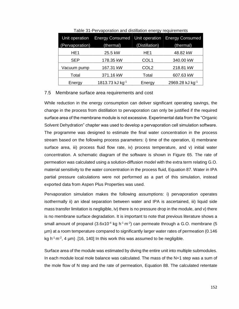
152

Table 31-Pervaporation and distillation energy requirements

Unit operation

(Pervaporation)

Energy Consumed

(thermal)

Unit operation

(Distillation)

Energy Consumed

(thermal)

HE1 25.5 kW HE1 48.82 kW

SEP 178.35 kW COL1 340.00 kW

Vacuum pump 167.31 kW COL2 218.81 kW

Total 371.16 kW Total 607.63 kW

Energy 1813.73 kJ kg-1 Energy 2969.28 kJ kg-1

7.5 Membrane surface area requirements and cost

While reduction in the energy consumption can deliver significant operating savings, the

change in the process from distillation to pervaporation can only be justified if the required

surface area of the membrane module is not excessive. Experimental data from the “Organic

Solvent Dehydration” chapter was used to develop a pervaporation cell simulation software.

The programme was designed to estimate the final water concentration in the process

stream based on the following process parameters: i) time of the operation, ii) membrane

surface area, iii) process fluid flow rate, iv) process temperature, and v) initial water

concentration. A schematic diagram of the software is shown in Figure 65. The rate of

permeation was calculated using a solution-diffusion model with the extra term relating G.O.

material sensitivity to the water concentration in the process fluid, Equation 87. Water in IPA

partial pressure calculations were not performed as a part of this simulation, instead

exported data from Aspen Plus Properties was used.

Pervaporation simulation makes the following assumptions: i) pervaporation operates

isothermally ii) an ideal separation between water and IPA is ascertained, iii) liquid side

mass transfer limitation is negligible, iv) there is no pressure drop in the module, and v) there

is no membrane surface degradation. It is important to note that previous literature shows a

small amount of propanol (3.6x10-4 kg h-1 m-2) can permeate through a G.O. membrane (5

µm) at a room temperature compared to significantly larger water rates of permeation (0.146

kg h-1 m-2, 4 µm) .[16, 140] In this work this was assumed to be negligible.

Surface area of the module was estimated by diving the entire unit into multiple submodules.

In each module local mole balance was calculated. The mass of the N+1 step was a sum of

the mole flow of N step and the rate of permeation, Equation 88. The calculated retentate

153

was then fed into the consecutive module until the number of user input steps was reached,

Equation 89. A schematic view of the theoretical model is shown in Figure 66 and Figure 67.

𝐽 = 𝑘𝑀.𝑃𝑥(𝑃 𝑊.𝐿 − 𝑃𝑊.𝑃) Equation 87

𝑛𝑓,𝑁+1 = 𝑛𝑓,𝑁 +𝑄𝑙𝑖𝑞𝑢𝑖𝑑 ∗ 𝐴

𝑀

Equation 88

𝑛𝑓,𝑁−1 = 𝑛𝑓,𝑁 , 𝑁 = 1, 2, 3, … … 𝑁 Equation 89

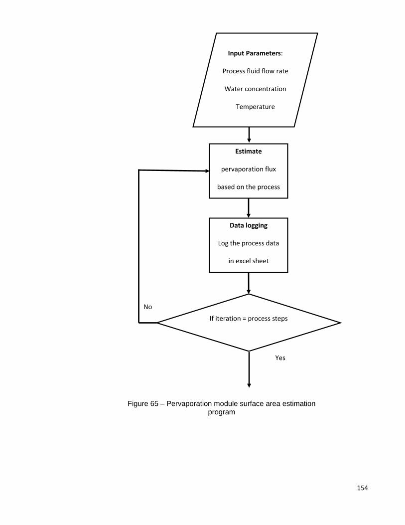
154

Input Parameters:

Process fluid flow rate

Water concentration

Temperature

Estimate

pervaporation flux

based on the process

Data logging

Log the process data

in excel sheet

If iteration = process steps

Yes

No

Figure 65 – Pervaporation module surface area estimation program

155

Figure 66 –Simulated pervaporation cell model[141]

Figure 67-Single block of a simulated pervaporation cell[141]

30 mbar

Stage N

Jwater, mol

N Jwater, mol

1 Jwater, mol

2

Stage 2 Stage 1 Process side

Permeate side

Direction of flow

Feed Retentate

Stage constants:

- Temperature - Pressure

Vacuum = 30 mbar

Single Element

(nf,N

)

nf,N-1

nf,N+1

Jwater, mol

156

The capital cost of a membrane module primarily depends on the total surface area

required. Several researchers have previously shown that a stand-alone membrane

process may require an excessively high surface area which creates large capital

expenditure and hinders the membrane process competitiveness.

An in-house built code was used to estimate the required membrane surface to

dehydrate 1000 kg/h of 30wt% water in IPA to a various degrees of dryness. A

pervaporation process using 2.1 µm G.O. membrane at 70°C was selected as this set of

conditions had robust set of data. The required surface area change with respect to the

final IPA concentration in the process solution is shown in Figure 68. There was a linear

increase in the total membrane required surface area up to 97wt%. In order to achieve

smaller amounts of water in the process solution the required surface area grows

exponentially. This was the result of a decrease in the driving force across the membrane

due to small water mole fraction on the retentate side. The effect is especially prominent

when G.O. membranes are used, because of its mole fraction square relationship to the

rate of permeation. However, this is not an unusual pervaporation membrane behaviour

and has been demonstrated in a previous research.[132] Despite the exponential growth

of the required surface, the feasibility of the process will be ultimately determined by the

capital cost of the membrane module.

In this case study the design specification of 5 wt% water in IPA could be achieved with

380 m2 membrane module. This is considered to be a small membrane operation. To the

extent of our knowledge the largest pervaporation operation to date has 3000 m2

membrane area.[8]

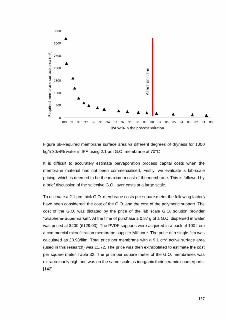
157

Figure 68-Required membrane surface area vs different degrees of dryness for 1000

kg/h 30wt% water in IPA using 2.1 µm G.O. membrane at 70°C

It is difficult to accurately estimate pervaporation process capital costs when the

membrane material has not been commercialised. Firstly, we evaluate a lab-scale

pricing, which is deemed to be the maximum cost of the membrane. This is followed by

a brief discussion of the selective G.O. layer costs at a large scale.

To estimate a 2.1 µm thick G.O. membrane costs per square meter the following factors

have been considered: the cost of the G.O. and the cost of the polymeric support. The

cost of the G.O. was dictated by the price of the lab scale G.O. solution provider

“Graphene-Supermarket”. At the time of purchase a 0.87 g of a G.O. dispersed in water

was priced at $200 (£129.03). The PVDF supports were acquired in a pack of 100 from

a commercial microfiltration membrane supplier Millipore. The price of a single film was

calculated as £0.98/film. Total price per membrane with a 9.1 cm2 active surface area

(used in this research) was £1.72. The price was then extrapolated to estimate the cost

per square meter, Table 32. The price per square meter of the G.O. membranes was

extraordinarily high and was on the same scale as inorganic their ceramic counterparts.

[142]

0

500

1000

1500

2000

2500

3000

3500

8081828384858687888990919293949596979899100

Req

uir

ed m

emb

ran

e su

rfac

e ar

ea (

m2)

IPA wt% in the process solution

Aze

otr

opic

lin

e

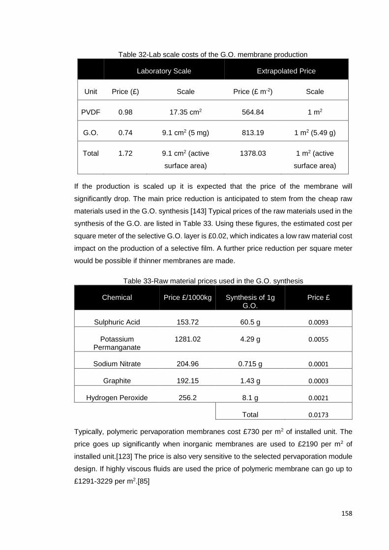
158

If the production is scaled up it is expected that the price of the membrane will

significantly drop. The main price reduction is anticipated to stem from the cheap raw

materials used in the G.O. synthesis [143] Typical prices of the raw materials used in the

synthesis of the G.O. are listed in Table 33. Using these figures, the estimated cost per

square meter of the selective G.O. layer is £0.02, which indicates a low raw material cost

impact on the production of a selective film. A further price reduction per square meter

would be possible if thinner membranes are made.

Table 33-Raw material prices used in the G.O. synthesis

Chemical Price £/1000kg Synthesis of 1g G.O.

Price £

Sulphuric Acid 153.72 60.5 g 0.0093

Potassium Permanganate

1281.02 4.29 g 0.0055

Sodium Nitrate 204.96 0.715 g 0.0001

Graphite 192.15 1.43 g 0.0003

Hydrogen Peroxide 256.2 8.1 g 0.0021

Total 0.0173

Typically, polymeric pervaporation membranes cost £730 per m2 of installed unit. The

price goes up significantly when inorganic membranes are used to £2190 per m2 of

installed unit.[123] The price is also very sensitive to the selected pervaporation module

design. If highly viscous fluids are used the price of polymeric membrane can go up to

£1291-3229 per m2.[85]

Table 32-Lab scale costs of the G.O. membrane production

Laboratory Scale Extrapolated Price

Unit Price (£) Scale Price (£ m-2) Scale

PVDF 0.98 17.35 cm2 564.84 1 m2

G.O. 0.74 9.1 cm2 (5 mg) 813.19 1 m2 (5.49 g)

Total 1.72 9.1 cm2 (active

surface area)

1378.03 1 m2 (active

surface area)

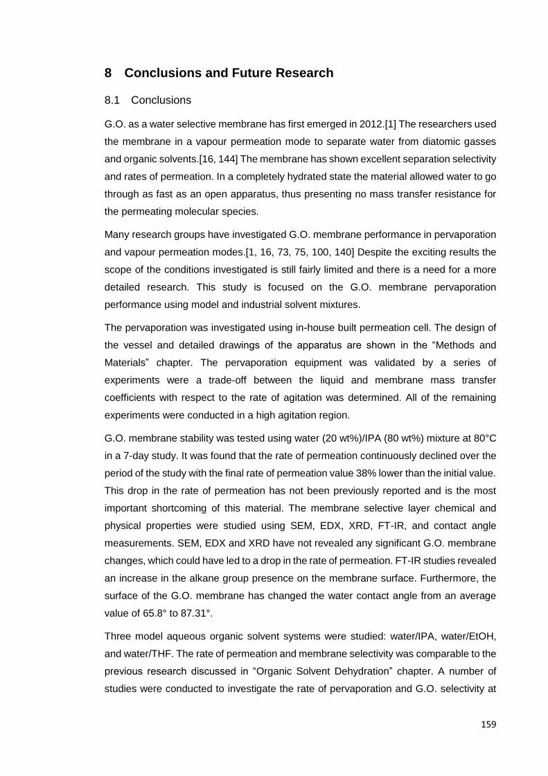
159

8 Conclusions and Future Research

8.1 Conclusions

G.O. as a water selective membrane has first emerged in 2012.[1] The researchers used

the membrane in a vapour permeation mode to separate water from diatomic gasses

and organic solvents.[16, 144] The membrane has shown excellent separation selectivity

and rates of permeation. In a completely hydrated state the material allowed water to go

through as fast as an open apparatus, thus presenting no mass transfer resistance for

the permeating molecular species.

Many research groups have investigated G.O. membrane performance in pervaporation

and vapour permeation modes.[1, 16, 73, 75, 100, 140] Despite the exciting results the

scope of the conditions investigated is still fairly limited and there is a need for a more

detailed research. This study is focused on the G.O. membrane pervaporation

performance using model and industrial solvent mixtures.

The pervaporation was investigated using in-house built permeation cell. The design of

the vessel and detailed drawings of the apparatus are shown in the “Methods and

Materials” chapter. The pervaporation equipment was validated by a series of

experiments were a trade-off between the liquid and membrane mass transfer

coefficients with respect to the rate of agitation was determined. All of the remaining

experiments were conducted in a high agitation region.

G.O. membrane stability was tested using water (20 wt%)/IPA (80 wt%) mixture at 80°C

in a 7-day study. It was found that the rate of permeation continuously declined over the

period of the study with the final rate of permeation value 38% lower than the initial value.

This drop in the rate of permeation has not been previously reported and is the most

important shortcoming of this material. The membrane selective layer chemical and

physical properties were studied using SEM, EDX, XRD, FT-IR, and contact angle

measurements. SEM, EDX and XRD have not revealed any significant G.O. membrane

changes, which could have led to a drop in the rate of permeation. FT-IR studies revealed

an increase in the alkane group presence on the membrane surface. Furthermore, the

surface of the G.O. membrane has changed the water contact angle from an average

value of 65.8° to 87.31°.

Three model aqueous organic solvent systems were studied: water/IPA, water/EtOH,

and water/THF. The rate of permeation and membrane selectivity was comparable to the

previous research discussed in “Organic Solvent Dehydration” chapter. A number of

studies were conducted to investigate the rate of pervaporation and G.O. selectivity at

160

low water concentrations in the process solution. A deviation from a linear Solution-

Diffusion model was found, which has not been reported previously. Interestingly, the

rate of permeation becomes linear if an additional term of the water mole fraction is

introduced. It is theorised that the non-linear relationship between rate of permeation and

partial water vapour pressure originates from a well-documented G.O. material solvation

by liquids such as water, EtOH and MeOH.[63] Overall, the G.O. membranes showed

excellent results in the water separation from organic liquids and had a similar

performance to the state-of-the-art and commercial pervaporation membranes,

“Industrial Case Studies”.

G.O. membrane potential in industrial applications was tested in the following case

studies: i) MeOH/n-Hexane separation, ii) dewatering of aqueous peptides, and iii) water

removal from an esterification of fatty carboxylic acid with IPA reaction mixture.

MeOH solvent separation was successful and the resulting permeate purity varied

between 93-99.2 wt%. This offers an opportunity to selectively separate polar and non-

polar solvent after second chromatographic separation step and improve the process by

reducing the solvent waste.

Esterification of fatty carboxylic acid and IPA was used to test in-situ water removal from

a reaction media. Initial experimentation showed a 19% increase in the yield compared

to a reaction without a selective water removal. A repeat of the study without replacing

the G.O. membrane resulted in a smaller 11% yield increase in the same time-frame.

The membrane was examined using SEM and EDX analytical techniques, which have

not shown any significant membrane changes compared to an unused G.O. membrane.

Membrane surface chemistry change was investigated using FT-IR. A set of peaks

emerged in the alkane C-H stretch region (2850-3000 cm-1). Contact angle

measurements showed a reduction in the surface hydrophilicity and an average contact

angle increase from 65.6° to 83.3°.

A high water permeation flux was demonstrated in peptide dewatering studies. Despite

good initial results G.O. membranes were prone to the peptide fouling and permeation

flux reduction. The presence of the surface foulants was confirmed by SEM and EDX.

Water contact angle measurements showed a reduction in the surface hydrophilicity.

Currently, it is not clear whether the membrane surface fouling is reversible or

irreversible. To elucidate whether permeation flux recovery is possible further research

is required.

Pervaporation data from organic solvent dewatering studies was used to create a

program which estimates the required surface area for a given water/IPA separation.

161

In addition, Aspen Plus was used to simulate pervaporation and extractive distillation of

water/IPA mixture and estimate the required energy for the separation. To make an

objective comparison between the process energy requirements to produce 1 kg of 95

wt% IPA was calculated. The extractive distillation process required 2.97 MJ kg-1 of IPA

produced while pervaporation process required 1.81 MJ kg-1. Pervaporation process

resulted in a 39% energy reduction, which would directly translate into operating cost

savings. Interestingly, vacuum pump energy consumption was a significant part of the

overall energy needs and contributed 45.08% to the overall IPA dewatering energy

budget. The energy requirements of the vacuum pump would be significantly smaller if

a lower vacuum is applied on the permeate side. However, this would result in a larger

membrane surface area requirement. It was estimated that 1000 kg h-1 30wt% water in

IPA mixture could be dehydrated to 95wt% IPA using 380 m 2 membrane module at 70°C.

Furthermore, it was found that due to G.O. material solvation by water the membrane

surface area requirements start growing exponentially once there was less than 3wt%

water in the process solution. This point marks a milestone beyond which alternative

membrane materials would hold an upper hand in terms of rate of permeation. While

G.O. membranes are less competitive at low water concentrations in the process solution

and have exponential growth of the required membrane area this can be potentially offset

by a cheap manufacturing costs. The raw materials used in the synthesis of the G.O. are

cheap bulk chemicals, which lead to incredibly low selective surface manufacturing costs

(0.02 £ m-1).

8.2 Future Research

The most important future research avenue is the reduction in the permeate flux at

elevated temperatures. A multi-layered G.O. membrane is known to have a minimal

functional group change up to 100°C. [103] XRD, SEM, and EDX studies have indicated

little to no change in the bulk of the material and physical appearance of the membrane.

Thus, the loss in activity has to be associated with the surface functional groups. The

issue has to be addressed before any further developments. A number of research

publications and several review papers have been published on the G.O. functional

group alteration.[57, 80, 145] This should serve as a prime source of information for a

stable G.O. membrane surface chemistry research.

G.O. material production

There have been individual attempts to demonstrate how various factors such as: i)

exfoliation, ii) parent graphite, and iii) oxidation methods, affects the final structure of the

G.O. material. [144, 146, 147] Furthermore, it has been demonstrated that the graphite

162

oxidation reaction can affect the solvation of the final product in powder and membrane

form.[63] Despite numerous individual research papers there is no published study which

relates previously discussed processing steps to the membrane selectivity of the rate of

permeation. Due to the size distribution of the parent graphite and non- homogeneously

distributed functional groups it is suggested to employ design of experiments to establish

the relationships between the membrane performance and its production route. This is

a large potential research area which can offer development of a more permeable and

selective G.O. based membrane.

G.O. selective layer is mechanically too fragile to be applied as a standalone membrane.

The issue is circumvented by preparing anisotropic membranes where the G.O. layer is

coated on a highly porous support. In this study G.O. was coated on a 70% porous

hydrophilic PVDF membrane. Many other supports have been used.[1, 16, 75, 100] Most

of them have been polymer based, which has given the flexible nature to the final

product. Initial research papers have also indicated a pervaporation rate and selectivity

difference among the G.O. membranes coated on different supports.[16] The reasons

behind the varying performance have not been elucidated. Thus, there is still room for a

more comprehensive study, which would bridge the gap between the nature of the

support and the selective layer performance. Perhaps the most impressive water rates

of permeation through G.O. membranes were demonstrated by a G.O. layer on a

ceramic support.[75] The G.O. membrane production on ceramic supports has not been

actively pursued and given the excellent results acquired in the prior publication this

could be a highly rewarding field of research.

Moving forward the membrane process should be scaled-up and tested. While research

in this body of work can serve as an excellent representation of a lab scale membrane

performance it does not capture the challenges of a large scale pervaporation process.

The most important issues to be addressed on a large scale G.O. membrane

manufacturing will be the coating technique. Several options are available: i) spin-

coating, ii) spray-coating, and iii) filtration-coating. It is not know which of these methods

can deliver the most uniform selective layer and minimal amount of defects. In this study

the thinnest membrane made had a 564 nm thick selective layer, which is larger than a

typical commercial membrane thickness.[85] To the best of our knowledge the thinnest

G.O. membrane had 97 nm thick selective layer which was coated on a thin film

nanocomposite support.[100] A significant amount of effort should be focused on making

the G.O. membranes thinner as this would significantly increase the rate of permeation.

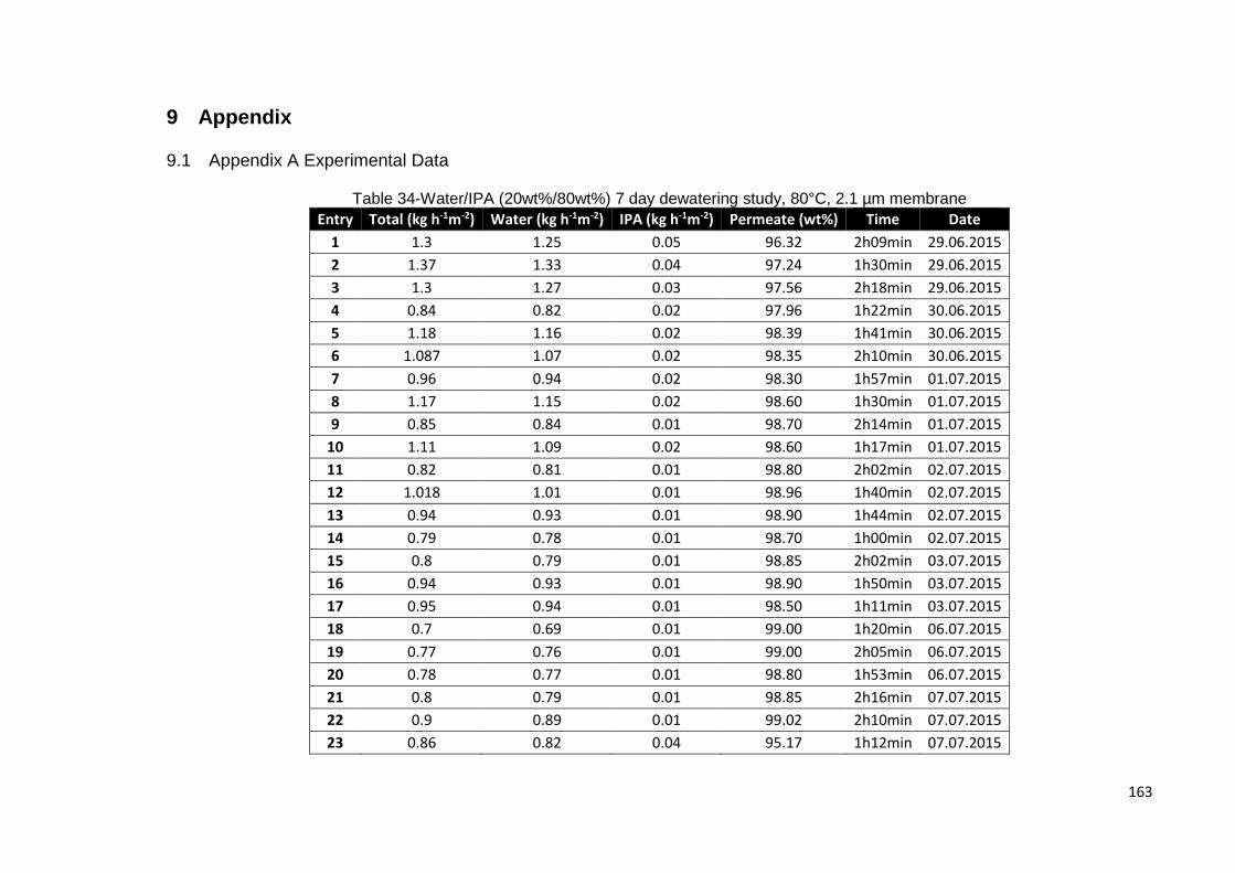
163

9 Appendix

9.1 Appendix A Experimental Data

Table 34-Water/IPA (20wt%/80wt%) 7 day dewatering study, 80°C, 2.1 µm membrane

Entry Total (kg h-1m-2) Water (kg h-1m-2) IPA (kg h-1m-2) Permeate (wt%) Time Date

1 1.3 1.25 0.05 96.32 2h09min 29.06.2015

2 1.37 1.33 0.04 97.24 1h30min 29.06.2015

3 1.3 1.27 0.03 97.56 2h18min 29.06.2015

4 0.84 0.82 0.02 97.96 1h22min 30.06.2015

5 1.18 1.16 0.02 98.39 1h41min 30.06.2015

6 1.087 1.07 0.02 98.35 2h10min 30.06.2015

7 0.96 0.94 0.02 98.30 1h57min 01.07.2015

8 1.17 1.15 0.02 98.60 1h30min 01.07.2015

9 0.85 0.84 0.01 98.70 2h14min 01.07.2015

10 1.11 1.09 0.02 98.60 1h17min 01.07.2015

11 0.82 0.81 0.01 98.80 2h02min 02.07.2015

12 1.018 1.01 0.01 98.96 1h40min 02.07.2015

13 0.94 0.93 0.01 98.90 1h44min 02.07.2015

14 0.79 0.78 0.01 98.70 1h00min 02.07.2015

15 0.8 0.79 0.01 98.85 2h02min 03.07.2015

16 0.94 0.93 0.01 98.90 1h50min 03.07.2015

17 0.95 0.94 0.01 98.50 1h11min 03.07.2015

18 0.7 0.69 0.01 99.00 1h20min 06.07.2015

19 0.77 0.76 0.01 99.00 2h05min 06.07.2015

20 0.78 0.77 0.01 98.80 1h53min 06.07.2015

21 0.8 0.79 0.01 98.85 2h16min 07.07.2015

22 0.9 0.89 0.01 99.02 2h10min 07.07.2015

23 0.86 0.82 0.04 95.17 1h12min 07.07.2015

164

Table 35-Water/IPA (30wt% / 70wt%) varying temperature (50-70°C) study, 2.1 µm membrane

Entry Temperature (°C) Total (kg h-1m-2) Water (kg h-1m-2) IPA (kg h-1m-2) Permeate (wt%) Date

1

70

1.39 1.36 0.03 97.60 26022014

2 1.48 1.44 0.03 97.70 26022014

3 1.40 1.37 0.03 97.60 26022014

4 1.42 1.39 0.03 98.20 26022014

5 1.33 1.29 0.04 97.20 26022014

6 1.49 1.47 0.02 98.80 26022014

7

60

0.91 0.91 0.00 99.99 15022014

8 0.85 0.85 0.00 99.99 15022014

9 1.04 1.03 0.00 99.99 15022014

10 1.00 1.00 0.00 99.99 15022014

11 0.94 0.94 0.00 99.99 15022014

12

50

0.58 0.58 0.00 99.99 17022014

13 0.76 0.76 0.00 99.99 17022014

14 0.60 0.59 0.00 99.99 17022014

15 0.76 0.76 0.00 99.99 17022014

16 0.80 0.79 0.01 99.30 18022014

17 0.90 0.90 0.00 99.99 18022014

18 0.86 0.86 0.00 99.99 18022015

19 0.51 0.51 0.00 99.99 18022015

20 0.67 0.67 0.01 99.00 18022015

21 0.61 0.59 0.01 98.00 18022015

22 0.69 0.68 0.01 99.13 18022015

23 0.84 0.83 0.01 99.15 18022015

24 0.77 0.76 0.01 99.20 18022015

165

Table 36-Water / EtOH (30wt% / 70wt%) varying temperature (50-80°C) study, 2.1 µm membrane


1

70

1.00 0.95 0.05 95.34 10.06.2015

2 1.03 0.98 0.05 95.46 10.06.2015

3 1.03 0.97 0.06 94.35 10.06.2015

4 50

0.40 0.38 0.02 95.03 15.06.2015

5 0.36 0.35 0.02 95.60 15.06.2015

6

80

1.21 1.16 0.05 95.64 15.06.2015

7 1.28 1.22 0.06 95.40 16.06.2015

8 1.13 1.08 0.05 96.01 16.06.2015

9 60

0.53 0.51 0.02 95.69 17.06.2015

10 0.54 0.51 0.02 95.65 17.06.2015

Table 37-Water / THF (30wt% / 70wt%) varying temperature (50-70°C) study, 1 µm membrane


1 60 1.61 1.573614 0.036386 97.74 09.04.2014

2 1.86 1.80606 0.05394 97.1 09.04.2014

3 1.83 1.78608 0.04392 97.6 09.04.2014

4 1.82 1.77996 0.04004 97.8 09.04.2014

5 50 1.12 1.1088 0.0112 99 09.04.2014

6 0.98 0.96138 0.01862 98.1 09.04.2014

7 1 0.992 0.008 99.2 09.04.2014

8 0.9 0.8928 0.0072 99.2 09.04.2014

9 70 2.96 2.92744 0.03256 98.9 09.04.2014

10 2.72 2.69552 0.02448 99.1 09.04.2014

11 2.9 2.8797 0.0203 99.3 09.04.2014

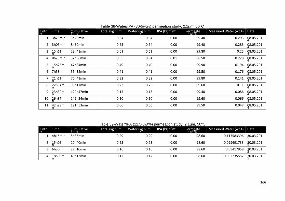
166

Table 38-Water/IPA (30-5wt%) permeation study, 2.1µm, 50°C

Entry

Time Cumulative Time

Total (kg h-1m-2)

Water (kg h-1m-2)

IPA (kg h-1m-2)

Permeate (wt%)

Measured Water (wt%) Date

1 3h23min 5h25min 0.64 0.64 0.00 99.40 0.293 08.05.2014

2 3h05min 8h30min 0.65 0.64 0.00 99.40 0.283 08.05.2014

3 15h11min

23h41min 0.61 0.61 0.00 99.80 0.25 08.05.2014

4 8h25min 32h06min 0.55 0.54 0.01 98.50 0.228 08.05.2014

5 15h25min

47h34min 0.49 0.49 0.00 99.90 0.194 08.05.2014

6 7h58min 55h32min 0.41 0.41 0.00 99.50 0.176 08.05.2014

7 21h11min

76h43min 0.32 0.32 0.00 99.80 0.141 08.05.2014

8 22h34min

99h17min 0.23 0.23 0.00 99.60 0.11 08.05.2014

9 23h30min

122h47min 0.15 0.15 0.00 99.40 0.086 08.05.2014

10 26h37min

149h24min 0.10 0.10 0.00 99.60 0.066 08.05.2014

11 42h29min

191h53min 0.06 0.05 0.00 99.50 0.047 08.05.2014

Table 39-Water/IPA (12.5-8wt%) permeation study, 2.1µm, 50°C

Entry


Total (kg h-1m-2)

Water (kg h-1m-2)

IPA (kg h-1m-2)

Permeate (wt%)


1 4h15min 5h35min 0.29 0.29 0.00 98.60 0.117583396 30.03.2015

2 15h05min

20h40min 0.23 0.23 0.00 98.60 0.099691733 30.03.2015

3 6h30min 27h10min 0.16 0.16 0.00 98.60 0.09417958 30.03.2015

4 18h03min

45h13min 0.12 0.12 0.00 98.60 0.082235557 30.03.2015

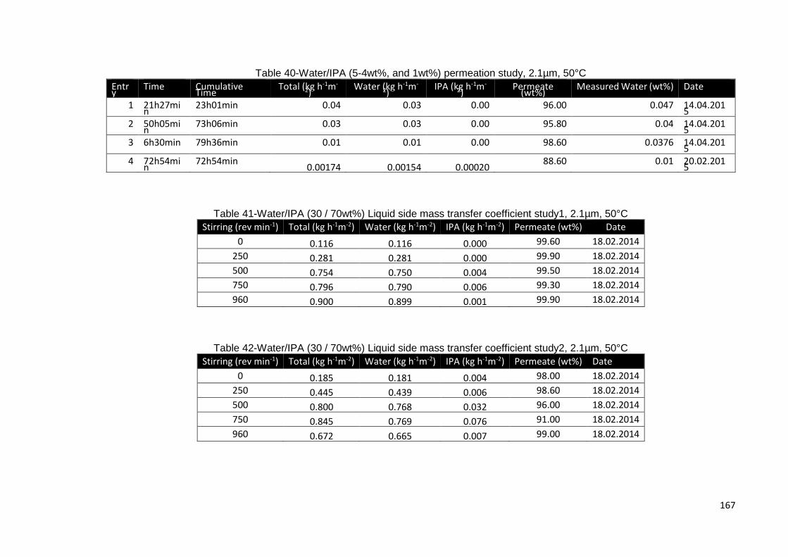
167

Table 40-Water/IPA (5-4wt%, and 1wt%) permeation study, 2.1µm, 50°C

Entry


Total (kg h-1m-2)

Water (kg h-1m-2)

IPA (kg h-1m-2)

Permeate (wt%)


1 21h27min

23h01min 0.04 0.03 0.00 96.00 0.047 14.04.2015

2 50h05min

73h06min 0.03 0.03 0.00 95.80 0.04 14.04.2015

3 6h30min 79h36min 0.01 0.01 0.00 98.60 0.0376 14.04.2015

4 72h54min

72h54min 0.00174 0.00154 0.00020

88.60 0.01 20.02.2015

Table 41-Water/IPA (30 / 70wt%) Liquid side mass transfer coefficient study1, 2.1µm, 50°C

Stirring (rev min-1) Total (kg h-1m-2) Water (kg h-1m-2) IPA (kg h-1m-2) Permeate (wt%) Date

0 0.116 0.116 0.000 99.60 18.02.2014

250 0.281 0.281 0.000 99.90 18.02.2014

500 0.754 0.750 0.004 99.50 18.02.2014

750 0.796 0.790 0.006 99.30 18.02.2014

960 0.900 0.899 0.001 99.90 18.02.2014



0 0.185 0.181 0.004 98.00 18.02.2014

250 0.445 0.439 0.006 98.60 18.02.2014

500 0.800 0.768 0.032 96.00 18.02.2014

750 0.845 0.769 0.076 91.00 18.02.2014

960 0.672 0.665 0.007 99.00 18.02.2014

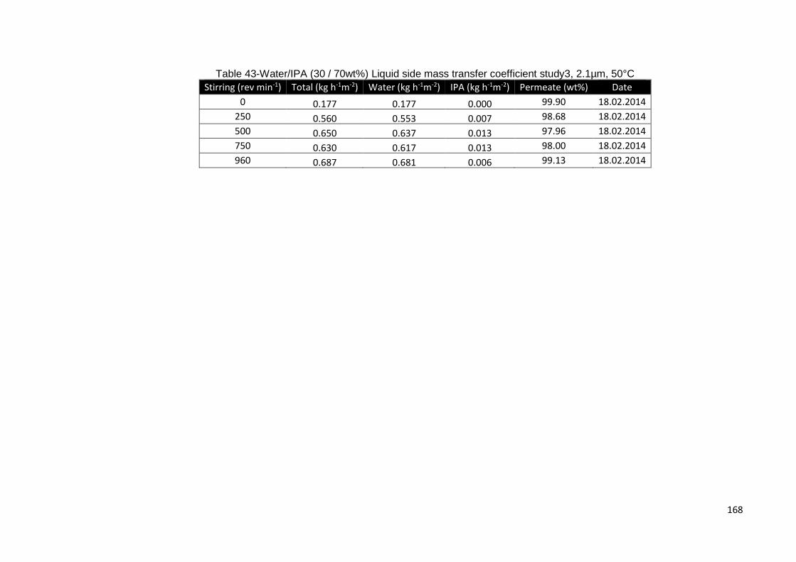
168



0 0.177 0.177 0.000 99.90 18.02.2014

250 0.560 0.553 0.007 98.68 18.02.2014

500 0.650 0.637 0.013 97.96 18.02.2014

750 0.630 0.617 0.013 98.00 18.02.2014

960 0.687 0.681 0.006 99.13 18.02.2014

169

Table 44-MeOH / n-Hexane pervaporation study, 2.1µm

Entry

MeOH (wt%)

n-Hexane (wt%)

Temperature (°C)

Total (kg h-1m-2)

MeOH (kg h-1m-2)

n-Hexane (kg h-1m-2)

Permeate (wt%)

Date

1 55 45

60

0.370 0.367 0.003 99.26 24.09.201

4

2 15 85

0.274 0.274 0.000 99.83 25.09.201

4

3 10 90

0.220 0.218 0.002 99.2 02.10.201

4

4 55 45

0.560 0.559 0.001 99.8 02.02.201

5

5 10 90

0.150 0.149 0.001 99.1 17.02.201

5

6 4 96 0.084 0.082 0.002 98.2 18.02.205

7 60 40

0.330 0.327 0.003 99 19.02.201

5

8 10 90

0.118 0.117 0.001 99.2 11.05.201

5

9 10 90

0.400 0.397 0.003 99.2 11.05.201

5

10 10 90

70

0.144 0.135 0.009 94 20.02.201

5

11 10 90

0.090 0.084 0.006 93 24.02.201

5

12 10 90

0.095 0.089 0.006 94 25.02.201

5

13 10 90

1.000 1.000 0.000 100 11.05.201

5

14 10 90

0.700 0.698 0.002 99.78 11.05.201

5

15 10 90

0.480 0.476 0.004 99.2 11.05.201

5

16 10 90

0.310 0.302 0.008 97.45 11.05.201

5

17 10 90

0.400 0.387 0.013 96.7 11.05.201

5

18 45 55

0.500 0.500 0.000 99.9 13.05.201

5

19 45 55

0.530 0.526 0.004 99.2 13.05.201

5

20 10 90 80 0.150 0.140 0.011

93 23.02.2015

170

Table 45-IPA and carboxylic acid esterification study1, 100°C, 2.1µm, 03.02.2015

Entry Sampling Time Cumulative Time Acid Value Conversion

1 0h00min 0h00min 4.87 0.00

2 1h13min 1h13min 4.23 13.14

3 2h23min 2h23min 3.53 27.52

4 3h37min 3h37min 2.83 41.89

5 5h30min 5h30min 2.17 55.44

6 1h32min 7h02min 1.75 64.07

7 2h30min 8h00min 1.62 66.74

8 3h53min 9h23min 1.5 69.20

9 5h22min 10h52min 1.38 71.66

10 6h06min 11h36min 1.33 72.69

11 1h29min 13h05min 1.24 74.54

12 2h35min 14h11min 1.22 74.95

13 4h23min 15h59min 1.16 76.18



1 0h00min 0h00min 4.9 0.00

2 1h20min 1h20min 4.27 12.86

3 2h31min 2h31min 3.51 28.37

4 3h33min 3h33min 3.08 37.14

5 5h18min 5h18min 2.64 46.12

6 1h43min 7h43min 2.1 57.14

7 3h00min 8h00min 1.86 62.04

8 4h41min 9h59min 1.71 65.10

9 6h30min 11h48min 1.68 65.71

10 1h51min 13h39min 1.56 68.16

11 4h16min 16h4min 1.5 69.39

12 5h46min 17h34min 1.43 70.82

13 6h48min 18h36min 1.49 69.59

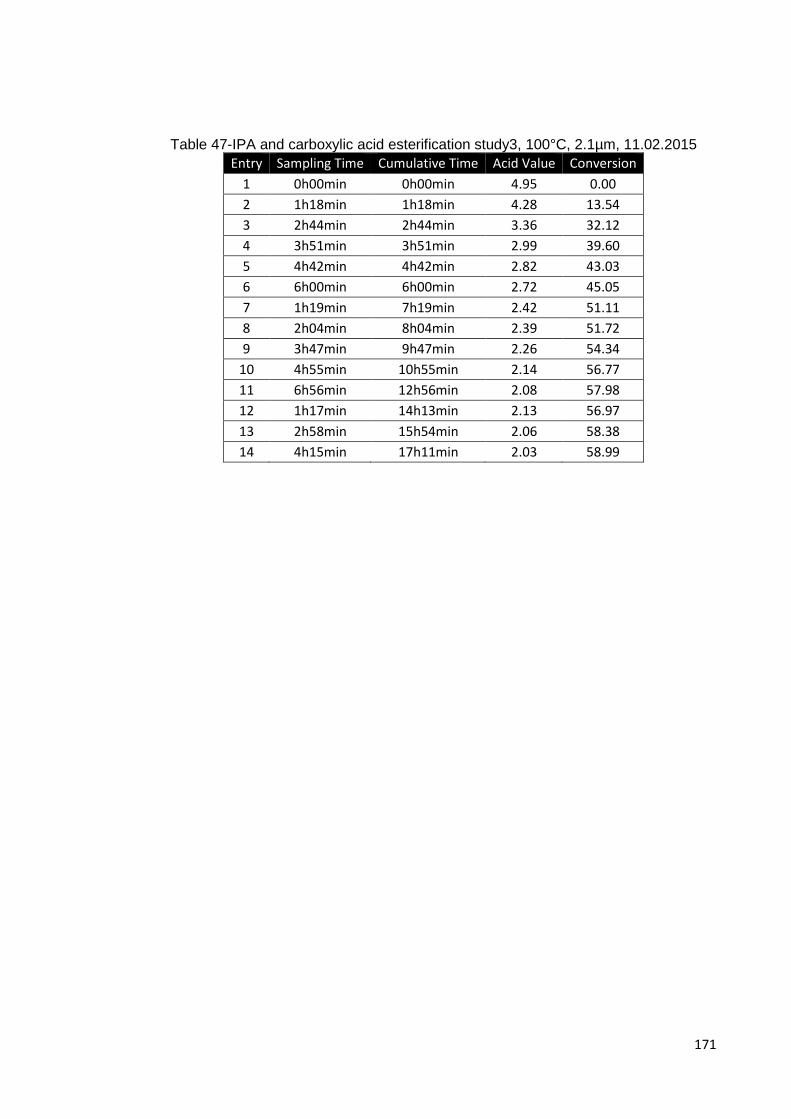
171



1 0h00min 0h00min 4.95 0.00

2 1h18min 1h18min 4.28 13.54

3 2h44min 2h44min 3.36 32.12

4 3h51min 3h51min 2.99 39.60

5 4h42min 4h42min 2.82 43.03

6 6h00min 6h00min 2.72 45.05

7 1h19min 7h19min 2.42 51.11

8 2h04min 8h04min 2.39 51.72

9 3h47min 9h47min 2.26 54.34

10 4h55min 10h55min 2.14 56.77

11 6h56min 12h56min 2.08 57.98

12 1h17min 14h13min 2.13 56.97

13 2h58min 15h54min 2.06 58.38

14 4h15min 17h11min 2.03 58.99

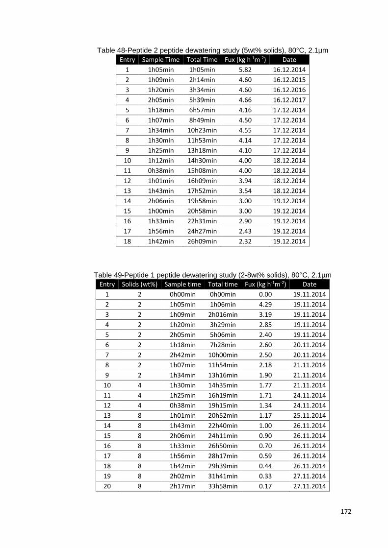
172

Table 48-Peptide 2 peptide dewatering study (5wt% solids), 80°C, 2.1µm

Entry Sample Time Total Time Fux (kg h-1m-2) Date

1 1h05min 1h05min 5.82 16.12.2014

2 1h09min 2h14min 4.60 16.12.2015

3 1h20min 3h34min 4.60 16.12.2016

4 2h05min 5h39min 4.66 16.12.2017

5 1h18min 6h57min 4.16 17.12.2014

6 1h07min 8h49min 4.50 17.12.2014

7 1h34min 10h23min 4.55 17.12.2014

8 1h30min 11h53min 4.14 17.12.2014

9 1h25min 13h18min 4.10 17.12.2014

10 1h12min 14h30min 4.00 18.12.2014

11 0h38min 15h08min 4.00 18.12.2014

12 1h01min 16h09min 3.94 18.12.2014

13 1h43min 17h52min 3.54 18.12.2014

14 2h06min 19h58min 3.00 19.12.2014

15 1h00min 20h58min 3.00 19.12.2014

16 1h33min 22h31min 2.90 19.12.2014

17 1h56min 24h27min 2.43 19.12.2014

18 1h42min 26h09min 2.32 19.12.2014

Table 49-Peptide 1 peptide dewatering study (2-8wt% solids), 80°C, 2.1µm

Entry Solids (wt%) Sample time Total time Fux (kg h-1m-2) Date

1 2 0h00min 0h00min 0.00 19.11.2014

2 2 1h05min 1h06min 4.29 19.11.2014

3 2 1h09min 2h016min 3.19 19.11.2014

4 2 1h20min 3h29min 2.85 19.11.2014

5 2 2h05min 5h06min 2.40 19.11.2014

6 2 1h18min 7h28min 2.60 20.11.2014

7 2 2h42min 10h00min 2.50 20.11.2014

8 2 1h07min 11h54min 2.18 21.11.2014

9 2 1h34min 13h16min 1.90 21.11.2014

10 4 1h30min 14h35min 1.77 21.11.2014

11 4 1h25min 16h19min 1.71 24.11.2014

12 4 0h38min 19h15min 1.34 24.11.2014

13 8 1h01min 20h52min 1.17 25.11.2014

14 8 1h43min 22h40min 1.00 26.11.2014

15 8 2h06min 24h11min 0.90 26.11.2014

16 8 1h33min 26h50min 0.70 26.11.2014

17 8 1h56min 28h17min 0.59 26.11.2014

18 8 1h42min 29h39min 0.44 26.11.2014

19 8 2h02min 31h41min 0.33 27.11.2014

20 8 2h17min 33h58min 0.17 27.11.2014

173

Table 50-Peptide 3 peptide dewatering study (2wt% solids), 70°C, 2.1µm, 07.01.2015

Entry Sample time Total time Fux (kg h-1m-2)

1 0h00min 0h00min 0

2 1h21min 1h21min 1.04

3 1h23min 2h44min 0.83

4 2h09min 4h53min 0.76

5 1h05min 5h58min 0.68

6 2h07min 7h20min 0.52

7 2h15min 9h27min 0.74

8 3h15min 12h42min 0.59

9 1h05min 13h47min 0.52

10 2h13min 16h01min 0.62

11 0h51min 16h52min 0.52

12 2h51min 18h52min 0.61

174

9.2 Appendix B Detailed Distillation Process Information

Column 1 Total number of stages 20 (including condenser and reboiler) IPA/Water Feed stage 16

IPA/Water Feed Flowrate (kg/h) 1000 IPA/Water Feed Composition (wt%) 70 (IPA) , 30 (H2O)

DMSO Feed Stage 3 DMSOP Feed Flowrate (kg/h) 289.4

Distillate Flowrate (kg/h) 736.84 Distillate Composition (wt%) 94.99 (IPA), 4.97 (H2O), 0.03 (DMSO)

Bottom Product Flowrate (kg/h) 552.56 Bottom Product Composition (wt%) 52.34 (DMSO), 47.65 (H2O), 0.00 (IPA)

Molar Reflux Ratio 1.088 Reboiler Duty 340.00kW

Condenser Duty -322.6 kW C1HE1

Inlet Hot (°C) 190.7 Outlet Hot (°C) 152.5 Inlet Cold (°C) 25

Outlet Cold (°C) 72 Heat Recovered (kW) 7.1

C1HE2 Inlet Hot (K) 200

Outlet Hot (K) 108.245 Inlet Cold (K) 25

Outlet Cold (K) 72 Heat Recovered (kW) 48.82

Column 2 Total number of stages 10 (including condenser and reboiler)

Feed stage 4 Feed Flowrate (kg/h) 552.56

Feed Composition (wt%) 52.34 (DMSO), 47.65 (H2O), 0.00 (IPA) Distillate Flowrate (kg/h) 263.32

Distillate Composition (wt%) 99.99 (H2O), 0.01 (DMSO) Bottom Product Flowrate (kg/h) 289.21

Bottom Product Composition (wt%) 99.99 (DMSO), 0.01 (H2O) Molar Reflux Ratio 0.3205 Reboiler Duty (kW) 218.80

Condenser Duty (kW) - 239.74

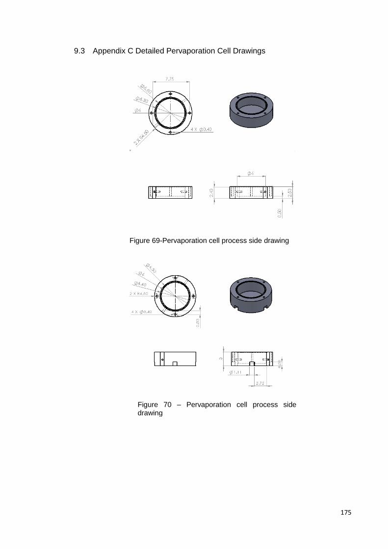
175

9.3 Appendix C Detailed Pervaporation Cell Drawings

Figure 69-Pervaporation cell process side drawing

Figure 70 – Pervaporation cell process side drawing

176

Figure 71 - Pervaporation cell membrane saddle drawing

Figure 72 - Pervaporation cell membrane saddle drawing

177

Figure 73-Porous stainless steel support drawing

Figure 74 –Stainless steel support drawing

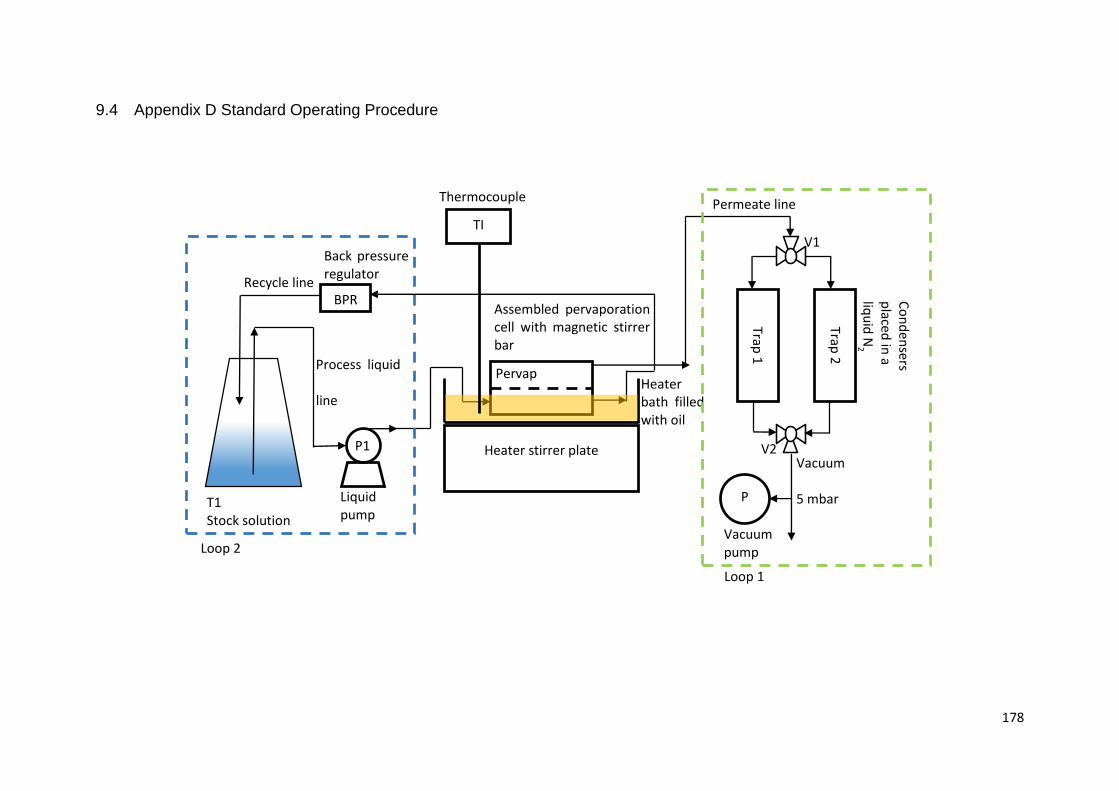
178

9.4 Appendix D Standard Operating Procedure

T1 Stock solution

Heater stirrer plate

Heater bath filled with oil

Assembled pervaporation cell with magnetic stirrer bar

Trap 1

Trap 2

Co

nd

ensers

placed

in a

liqu

id N

2

Vacuum

5 mbar

Recycle line

Permeate line

Process liquid

line

TI

Thermocouple

V1

V2

BPR

Back pressure regulator

Liquid pump

P

Vacuum pump

Pervap

P1

Loop 2

Loop 1

179

Start up

Loop 1

1. Ensure that valve 1 (V1) and valve 2 (V2) are completely closed.

2. Turn on the vacuum pump (P2), and wait until the operating line is under

vacuum

3. Open the desired operating line using a three way valve (valve 2); wait until the

line is under vacuum.

4. Initiate the remainder of the line by operating a three way valve (valve 1); wait

until the line is under vacuum. At this stage the desired operating line is under

vacuum conditions

5. Proceed to the “Loop 2”

180

Loop 2

1. Close pervaporation cell’s outlet and inlet. Wait for 10 minutes and measure the

pressure inside the pervaporation cell’s process side. A significant drop in

pressure indicates either a flaw on a membrane surface or incorrectly fitted

membrane. Resolve the pressure drop before proceeding further.

2. Load the conical flask (T1) with desired amount and composition liquid

3. Switch on the pump (P1) and fill the pervaporation cell

4. Place the pervaporation cell in a hot oil bath located on a heater stirrer plate.

5. Initiate stirring on a heater stirrer plate

6. Lower the cold finger connected to a vacuum line into a liquid nitrogen dewar

Sampling

1. Isolate the cold finger submerged into a liquid nitrogen using V1 and V2. Lift it

out of the drawer

2. Initiate vacuum on the parallel line by operating V1 and V2. Wait until the

pressure gauge indicates that the line is under vacuum.

3. Lower the cold finger into the liquid nitrogen dewar

4. Wait until the sample is in a liquid phase in the cold finger and then extract it

using a syringe and a needle

5. Weight and analyse the sample

Shutdown

1. Close both three way valves (V 1 and V 2)

2. Ensure both cold fingers are lifted up and are not in contact with the liquid

nitrogen

3. Stop the vacuum pump (P2)

4. Stop the liquid pump (P1)

5. Lift the pervaporation cell out of the oil bath and drain the liquid from the inside

6. Ensure all electrical appliances are switched off

181

Notes

1. The direction of the arrow on a three way valve indicates the direction of the

flow.

2. When the arrow is not pointing to either of the sides the valve is in its closed

position

3. Ensure pump has upper and lower pressure cut off limits set

4. The back pressure regulator rating must not be lower than the lowest pressure

limit or higher than the highest pressure limit. If these conditions are not met

pump will not operate

5. Check both cold fingers for any chips and cracks before operating the

apparatus

182

10 Reference

1. Nair, R.R., et al., Unimpeded Permeation of Water Through Helium-Leak–Tight Graphene-Based Membranes. Science, 2012. 335(6067): p. 442-444.

2. Wijmans, J.G. and R.W. Baker, The solution-diffusion model: a review. J. Membr. Sci., 1995. 107: p. 1-21.

3. Wei, N., X. Peng, and Z. Xu, Understanding Water Permeation in Graphene Oxide Membranes. ACS Applied Materials & Interfaces, 2014. 6(8): p. 5877-5883.

4. Höök, M. and X. Tang, Depletion of fossil fuels and anthropogenic climate change—A review. Energy Policy, 2013. 52(0): p. 797-809.

5. Durbin, J., A 'whole building' path to climate control. Health Estate, 2010. 64: p. 71-3.

6. Babi, D.K., et al., Sustainable process synthesis–intensification. Computers & Chemical Engineering, (0).

7. Van Gerven, T. and A. Stankiewicz, Structure, Energy, Synergy, Time—The Fundamentals of Process Intensification. Industrial & Engineering Chemistry Research, 2009. 48(5): p. 2465-2474.

8. Servel, C., et al., Improved Energy Efficiency of a Hybrid Pervaporation/Distillation Process for Acetic Acid Production: Identification of Target Membrane Performances by Simulation. Industrial & Engineering Chemistry Research, 2014.

9. Commissions, E., Membrane technologies for water applications, in Highlights from a selection of European research projects. 2010.

10. Diban, N., et al., Membrane Reactors for in Situ Water Removal: A Review of Applications. Industrial & Engineering Chemistry Research, 2013. 52(31): p. 10342-10354.

11. Baker, R.W., Membrane Technology and Applications. 2012: Wiley.

12. Joo, S.H. and B. Tansel, Novel technologies for reverse osmosis concentrate treatment: A review. Journal of Environmental Management, 2015. 150: p. 322-335.

13. Mahdi, T., et al., State-of-the-Art Technologies for Separation of Azeotropic Mixtures. Separation & Purification Reviews, 2014. 44(4): p. 308-330.

14. Chapman, P.D., et al., Membranes for the dehydration of solvents by pervaporation. Journal of Membrane Science, 2008. 318(1–2): p. 5-37.

15. Zhao, J., et al., Fabricating graphene oxide-based ultrathin hybrid membrane for pervaporation dehydration via layer-by-layer self-assembly driven by multiple interactions. Journal of Membrane Science, 2015. 487(Copyright (C) 2015 American Chemical Society (ACS). All Rights Reserved.): p. 162-172.

16. Nair, R., P. Budd, and A. Geim, Separation of water using a membrane. 2014, Google Patents.

17. Tang, Y.P., D.R. Paul, and T.S. Chung, Free-standing graphene oxide thin films assembled by a pressurized ultrafiltration method for dehydration of ethanol. Journal of Membrane Science, 2014. 458(0): p. 199-208.

18. Shao, P. and R.Y.M. Huang, Polymeric membrane pervaporation. Journal of Membrane Science, 2007. 287(2): p. 162-179.

183

19. Smitha, B., et al., Separation of organic–organic mixtures by pervaporation—a review. Journal of Membrane Science, 2004. 241(1): p. 1-21.

20. Guo, W.F., T.-S. Chung, and T. Matsuura, Pervaporation study on the dehydration of aqueous butanol solutions: a comparison of flux vs. permeance, separation factor vs. selectivity. Journal of Membrane Science, 2004. 245(1–2): p. 199-210.

21. Kanti, P., et al., Dehydration of ethanol through blend membranes of chitosan and sodium alginate by pervaporation. Separation and Purification Technology, 2004. 40(3): p. 259-266.

22. Sander, U. and P. Soukup, Design and operation of a pervaporation plant for ethanol dehydration. J. Membr. Sci., 1988. 36(Copyright (C) 2012 American Chemical Society (ACS). All Rights Reserved.): p. 463-75.

23. Bolto, B., M. Hoang, and Z. Xie, A review of membrane selection for the dehydration of aqueous ethanol by pervaporation. Chem. Eng. Process., 2011. 50: p. 227-235.

24. Zhang, L., et al., Ion exchange membranes blended by cellulose cuoxam with alginate. Journal of Membrane Science, 1997. 124(2): p. 195-201.

25. Yeom, C.K. and K.H. Lee, Vapor permeation of ethanol-water mixtures using sodium alginate membranes with crosslinking gradient structure. Journal of Membrane Science, 1997. 135(2): p. 225-235.

26. Yang, G., et al., Effects of Ca2+ bridge cross-linking on structure and pervaporation of cellulose/alginate blend membranes. Journal of Membrane Science, 2000. 175(1): p. 53-60.

27. Gimenes, M.L., L. Liu, and X. Feng, Sericin/poly(vinyl alcohol) blend membranes for pervaporation separation of ethanol/water mixtures. Journal of Membrane Science, 2007. 295(1–2): p. 71-79.

28. Am, E.D.J. and Editor, Chemical Engineering In The Pharmaceutical Industry: R & D To Manufacturing. 2011: John Wiley & Sons, Inc. 887 pp.

29. See Toh, Y.H., F.W. Lim, and A.G. Livingston, Polymeric membranes for nanofiltration in polar aprotic solvents. Journal of Membrane Science, 2007. 301(1–2): p. 3-10.

30. Verkerk, A.W., et al., Properties of high flux ceramic pervaporation membranes for dehydration of alcohol/water mixtures. Separation and Purification Technology, 2001. 22–23(0): p. 689-695.

31. Svang-Ariyaskul, A., et al., Blended chitosan and polyvinyl alcohol membranes for the pervaporation dehydration of isopropanol. Journal of Membrane Science, 2006. 280(1–2): p. 815-823.

32. Huang, R.Y.M. and Editor, Membrane Science and Technology Series, 1: Pervaporation Membrane Separation Processes. 1991: Elsevier. 549 pp.

33. Ge, J., et al., The effect of structure on pervaporation of chitosan membrane. Journal of Membrane Science, 2000. 165(1): p. 75-81.

34. Huang, Z., et al., Pervaporation study of aqueous ethanol solution through zeolite-incorporated multilayer poly(vinyl alcohol) membranes: Effect of zeolites. Journal of Membrane Science, 2006. 276(1–2): p. 260-271.

35. Lee, K.-R., R.-Y. Chen, and J.-Y. Lai, Plasma deposition of vinyl acetate onto Nylon-4 membrane for pervaporation and evapomeation separation of aqueous alcohol mixtures. Journal of Membrane Science, 1992. 75(1–2): p. 171-180.

184

36. Yeom, C.K. and K.H. Lee, Characterization of sodium alginate and poly(vinyl alcohol) blend membranes in pervaporation separation. Journal of Applied Polymer Science, 1998. 67(5): p. 949-959.

37. Bettens, B., et al., Transport of Pure Components in Pervaporation through a Microporous Silica Membrane. The Journal of Physical Chemistry B, 2005. 109(11): p. 5216-5222.

38. Yu, J., et al., Method for producing hollow molecular sieve fiber having microporous-mesoporous-macroporous structure by coaxial spinning. 2008, Jilin University, Peop. Rep. China . p. 20pp.

39. Verkerk, A.W., et al., Description of dehydration performance of amorphous silica pervaporation membranes. Journal of Membrane Science, 2001. 193(2): p. 227-238.

40. Sommer, S. and T. Melin, Influence of operation parameters on the separation of mixtures by pervaporation and vapor permeation with inorganic membranes. Part 1: Dehydration of solvents. Chemical Engineering Science, 2005. 60(16): p. 4509-4523.

41. van Gemert, R.W. and F. Petrus Cuperus, Newly developed ceramic membranes for dehydration and separation of organic mixtures by pervaporation. Journal of Membrane Science, 1995. 105(3): p. 287-291.

42. Sekulić, J., et al., Microporous silica and doped silica membrane for alcohol dehydration by pervaporation. Desalination, 2002. 148(1–3): p. 19-23.

43. Okamoto, K.-i., H. Kita, and K. Horii, Zeolite NaA Membrane: Preparation, Single-Gas Permeation, and Pervaporation and Vapor Permeation of Water/Organic Liquid Mixtures. Industrial & Engineering Chemistry Research, 2000. 40(1): p. 163-175.

44. Kondo, M., et al., Tubular-type pervaporation module with zeolite NaA membrane. Journal of Membrane Science, 1997. 133(1): p. 133-141.

45. Hasegawa, Y., et al., Influence of acid on the permeation properties of NaA-type zeolite membranes. Journal of Membrane Science, 2010. 349(1–2): p. 189-194.

46. van Veen, H.M., et al., Pushing membrane stability boundaries with HybSi® pervaporation membranes. Journal of Membrane Science, 2011. 380(1–2): p. 124-131.

47. Agirre, I., et al., Acetalization reaction of ethanol with butyraldehyde coupled with pervaporation. Semi-batch pervaporation studies and resistance of HybSi® membranes to catalyst impacts. Journal of Membrane Science, 2011. 371(1–2): p. 179-188.

48. Liu, G., et al., Polymer/Ceramic Composite Membranes and Their Application in Pervaporation Process. Chin. J. Chem. Eng., 2012. 20(1): p. 62-70.

49. Gao, Z., Y. Yue, and W. Li, Application of zeolite-filled pervaporation membrane. Zeolites, 1996. 16(1): p. 70-74.

50. Zhang, Q.G., et al., Dehydration of Isopropanol by Novel Poly(vinyl alcohol)−Silicone Hybrid Membranes. Industrial & Engineering Chemistry Research, 2007. 46(3): p. 913-920.

51. Kariduraganavar, M.Y., et al., Organic−Inorganic Hybrid Membranes: Solving the Trade-off Phenomenon Between Permeation Flux and Selectivity in Pervaporation. Industrial & Engineering Chemistry Research, 2009. 48(8): p. 4002-4013.

185

52. Uragami, T., et al., Structure and Permeation Characteristics of an Aqueous Ethanol Solution of Organic−Inorganic Hybrid Membranes Composed of Poly(vinyl alcohol) and Tetraethoxysilane. Macromolecules, 2002. 35(24): p. 9156-9163.

53. White, L.S., Development of large-scale applications in organic solvent nanofiltration and pervaporation for chemical and refining processes. Journal of Membrane Science, 2006. 286(1–2): p. 26-35.

54. Morigami, Y., et al., The first large-scale pervaporation plant using tubular-type module with zeolite NaA membrane. Separation and Purification Technology, 2001. 25(1–3): p. 251-260.

55. Hasanoglu, A., et al., The esterification of acetic acid with ethanol in a pervaporation membrane reactor. Desalination, 2009. 245: p. 662-669.

56. Waldburger, R.M. and F. Widmer, Membrane reactors in chemical production processes and the application to the pervaporation-assisted esterification. Chemical Engineering & Technology, 1996. 19(2): p. 117-126.

57. Dreyer, D.R., et al., The chemistry of graphene oxide. Chemical Society Reviews, 2010. 39(1): p. 228-240.

58. Huang, H., Y. Ying, and X. Peng, Graphene oxide nanosheet: an emerging star material for novel separation membranes. Journal of Materials Chemistry A, 2014. 2(34): p. 13772-13782.

59. He, H., et al., Solid-State NMR Studies of the Structure of Graphite Oxide. The Journal of Physical Chemistry, 1996. 100(51): p. 19954-19958.

60. Szabó, T., et al., Evolution of Surface Functional Groups in a Series of Progressively Oxidized Graphite Oxides. Chemistry of Materials, 2006. 18(11): p. 2740-2749.

61. Dikin, D.A., et al., Preparation and characterization of graphene oxide paper. Nature, 2007. 448(7152): p. 457-460.

62. Paredes, J.I., et al., Graphene Oxide Dispersions in Organic Solvents. Langmuir, 2008. 24(19): p. 10560-10564.

63. Talyzin, A.V., et al., The structure of graphene oxide membranes in liquid water, ethanol and water-ethanol mixtures. Nanoscale, 2014. 6(1): p. 272-281.

64. Huang, H., et al., Ultrafast viscous water flow through nanostrand-channelled graphene oxide membranes. Nat Commun, 2013. 4.

65. Dong, Z., et al., High performance ceramic hollow fiber supported PDMS composite pervaporation membrane for bio-butanol recovery. Journal of Membrane Science, 2014. 450(0): p. 38-47.

66. Brodie, B.C., On the Atomic Weight of Graphite. Philosophical Transactions of the Royal Society of London, 1859. 149: p. 249-259.

67. Hummers, W.S. and R.E. Offeman, Preparation of Graphitic Oxide. Journal of the American Chemical Society, 1958. 80(6): p. 1339-1339.

68. Marcano, D.C., et al., Improved Synthesis of Graphene Oxide. ACS Nano, 2010. 4(8): p. 4806-4814.

69. Chen, J., et al., An improved Hummers method for eco-friendly synthesis of graphene oxide. Carbon, 2013. 64(0): p. 225-229.

70. Berg, D. and L.C. Flowers, Graphitic oxide memberane for desalinating water. 1969, Google Patents.

186

71. Yeh, T.-M., et al. High flux ethanol dehydration using multilayered graphene oxide membranes. 2013. American Chemical Society.

72. Yeh, T.-M., et al., Polymeric nanofibrous composite membranes for energy efficient ethanol dehydration. J. Renewable Sustainable Energy, 2012. 4: p. 041406/1-041406/9.

73. Liu, R., et al., Graphene oxide membrane for liquid phase organic molecular separation. Carbon, 2014. 77(0): p. 933-938.

74. Tang, Y., et al., Development of flat-sheet membranes for C1–C4 alcohols dehydration via pervaporation from sulfonated polyphenylsulfone (sPPSU). Journal of Membrane Science, 2012. 415–416(0): p. 686-695.

75. Huang, K., et al., A Graphene Oxide Membrane with Highly Selective Molecular Separation of Aqueous Organic Solution. Angewandte Chemie International Edition, 2014. 53(27): p. 6929-6932.

76. Qiao, X., et al., Dehydration of isopropanol and its comparison with dehydration of butanol isomers from thermodynamic and molecular aspects. Journal of Membrane Science, 2005. 252(1–2): p. 37-49.

77. Okada, T. and T. Matsuura, A new transport model for pervaporation. Journal of Membrane Science, 1991. 59(2): p. 133-149.

78. Sukitpaneenit, P., T.-S. Chung, and L.Y. Jiang, Modified pore-flow model for pervaporation mass transport in PVDF hollow fiber membranes for ethanol–water separation. Journal of Membrane Science, 2010. 362(1–2): p. 393-406.

79. Gilliland, E.R., R.F. Baddour, and J.L. Russell, Rates of flow through microporous solids. AIChE Journal, 1958. 4(1): p. 90-96.

80. Jia, Z. and Y. Wang, Covalently crosslinked graphene oxide membranes by esterification reactions for ions separation. Journal of Materials Chemistry A, 2015. 3(8): p. 4405-4412.

81. Okada, T., M. Yoshikawa, and T. Matsuura, A study on the pervaporation of ethanol/water mixtures on the basis of pore flow model. Journal of Membrane Science, 1991. 59(2): p. 151-168.

82. Wijmans, J.G. and R.W. Baker, A simple predictive treatment of the permeation process in pervaporation. Journal of Membrane Science, 1993. 79(1): p. 101-113.

83. Wijmans, J.G., et al., The role of boundary layers in the removal of volatile organic compounds from water by pervaporation. J. Membr. Sci., 1996. 109: p. 135-46.

84. Bridgeman, O.C. and E.W. Aldrich, Vapor Pressure Tables for Water. Journal of Heat Transfer, 1964. 86(2): p. 279-286.

85. Baker, R., Membrane Technology and Applications, 2nd Edition. 2004: John Wiley & Sons. 568 pp.

86. Feng, X. and R.Y.M. Huang, Concentration polarization in pervaporation separation processes. Journal of Membrane Science, 1994. 92(3): p. 201-208.

87. Bhattacharya, S. and S.-T. Hwang, Concentration polarization, separation factor, and Peclet number in membrane processes. Journal of Membrane Science, 1997. 132(1): p. 73-90.

88. Nagy, E. and E. Kulcsar, The effect of the concentration polarization and the membrane layer mass transport on membrane separation. Desalin. Water Treat., 2010. 14: p. 220-226.

187

89. Jaffrin, M.Y., B.B. Gupta, and P. Paullier, Energy saving pulsatile mode cross flow filtration. Journal of Membrane Science, 1994. 86(3): p. 281-290.

90. Da Costa, A.R., A.G. Fane, and D.E. Wiley, Spacer characterization and pressure drop modelling in spacer-filled channels for ultrafiltration. Journal of Membrane Science, 1994. 87(1–2): p. 79-98.

91. Nagy, E., Coupled effect of the membrane properties and concentration polarization in pervaporation: unified mass transport model. Separation and Purification Technology, 2010. 73: p. 194-201.

92. Jiraratananon, R., A. Chanachai, and R.Y.M. Huang, Pervaporation dehydration of ethanol–water mixtures with chitosan/hydroxyethylcellulose (CS/HEC) composite membranes: II. Analysis of mass transport. Journal of Membrane Science, 2002. 199(1–2): p. 211-222.

93. Schofield, R.W., A.G. Fane, and C.J.D. Fell, Gas and vapour transport through microporous membranes. I. Knudsen-Poiseuille transition. Journal of Membrane Science, 1990. 53(1–2): p. 159-171.

94. Noworyta, A., M. Kubasiewicz-Ponitka, and A. Koziol, Mass and heat transport resistance in pervaporation process. Desalination and Water Treatment, 2011. 26(1-3): p. 226-235.

95. Cavanagh, E.J., M.J. Savelski, and C.S. Slater, Optimization of environmental impact reduction and economic feasibility of solvent waste recovery using a new software tool. Chemical Engineering Research and Design, 2014. 92(10): p. 1942-1954.

96. Baker, R.W., et al., The effect of concentration polarization on the separation of volatile organic compounds from water by pervaporation. Journal of Membrane Science, 1997. 137(1–2): p. 159-172.

97. Taherian, F., et al., What Is the Contact Angle of Water on Graphene? Langmuir, 2013. 29(5): p. 1457-1465.

98. Hao, L. and D.G. Leaist, Binary Mutual Diffusion Coefficients of Aqueous Alcohols. Methanol to 1-Heptanol. Journal of Chemical and Engineering Data, 1996. 41(2): p. 210-213.

99. Li, H., et al., Ultrathin, Molecular-Sieving Graphene Oxide Membranes for Selective Hydrogen Separation. Science, 2013. 342(6154): p. 95-98.

100. Yeh, T.-M., et al., High Flux Ethanol Dehydration using Nanofibrous Membranes Containing Graphene Oxide Barrier Layer. Journal of Materials Chemistry A, 2013.

101. Bayer, T., et al., Characterization of a graphene oxide membrane fuel cell. Journal of Power Sources, 2014. 272: p. 239-247.

102. Shen, J., et al., Fast and Facile Preparation of Graphene Oxide and Reduced Graphene Oxide Nanoplatelets. Chem. Mater., 2009. 21: p. 3514-3520.

103. Acik, M., et al., The role of oxygen during thermal reduction of graphene oxide studied by infrared absorption spectroscopy. The Journal of Physical Chemistry C, 2011. 115(40): p. 19761-19781.

104. Bian, J., et al., Processing and assessment of high-performance poly(butylene terephthalate) nanocomposites reinforced with microwave exfoliated graphite oxide nanosheets. Eur. Polym. J., 2013. 49: p. 1406-1423.

188

105. Kumarasinghe, A.R., et al., Self-Assembled Multilayer Graphene Oxide Membrane and Carbon Nanotubes Synthesized Using a Rare Form of Natural Graphite. J. Phys. Chem. C, 2013. 117: p. 9507-9519.

106. Jeong, H.-K., et al., Thermal stability of graphite oxide. Chem. Phys. Lett., 2009. 470: p. 255-258.

107. Gong, C., et al., Graphitization of Graphene Oxide with Ethanol during Thermal Reduction. The Journal of Physical Chemistry C, 2012. 116(18): p. 9969-9979.

108. Wang, A.-X., et al., Preparation and characterization of novel spica-like hierarchical vaterite calcium carbonate and a hydrophilic poly(vinylidene fluoride)/calcium carbonate composite membrane. CrystEngComm, 2014. 16(24): p. 5198-5205.

109. Rattana, et al., Preparation and characterization of graphene oxide nanosheets. Procedia Engineering, 2012. 32(0): p. 759-764.

110. Szabó, T., et al., Enhanced acidity and pH-dependent surface charge characterization of successively oxidized graphite oxides. Carbon, 2006. 44(3): p. 537-545.

111. Zuo, P.-P., et al., Fabrication of biocompatible and mechanically reinforced graphene oxide-chitosan nanocomposite films. Chemistry Central Journal, 2013. 7(1): p. 39.

112. Deshmukh, K. and G.M. Joshi, Novel nanocomposites of graphene oxide reinforced poly (3,4-ethylenedioxythiophene)-block-poly (ethylene glycol) and polyvinylidene fluoride for embedded capacitor applications. RSC Advances, 2014. 4(71): p. 37954-37963.

113. Han, Y.-J., et al., Hydrophilic chitosan-modified polybenzoimidazole membranes for pervaporation dehydration of isopropanol aqueous solutions. Journal of Membrane Science, 2014. 463(0): p. 17-23.

114. Ganetsos, G. and P.E. Barker, Large-scale chromatography in industrial processing. Journal of Chemical Technology & Biotechnology, 1991. 50(1): p. 101-108.

115. Pei, S., et al., Direct reduction of graphene oxide films into highly conductive and flexible graphene films by hydrohalic acids. Carbon, 2010. 48(15): p. 4466-4474.

116. Peng, X., et al., Zeolite membrane-assisted preparation of high fatty esters. Separation and Purification Technology, 2012. 89: p. 84-90.

117. Korkmaz, S., Y. Salt, and S. Dincer, Esterification of Acetic Acid and Isobutanol in a Pervaporation Membrane Reactor Using Different Membranes. Ind. Eng. Chem. Res., 2011. 50: p. 11657-11666.

118. Paradis, G.G., et al., From hydrophilic to hydrophobic HybSi® membranes: A change of affinity and applicability. Journal of Membrane Science, 2013. 428: p. 157-162.

119. Zinadini, S., et al., Preparation of a novel antifouling mixed matrix PES membrane by embedding graphene oxide nanoplates. Journal of Membrane Science, 2014. 453: p. 292-301.

120. Chan, R. and V. Chen, Characterization of protein fouling on membranes: opportunities and challenges. Journal of Membrane Science, 2004. 242(1–2): p. 169-188.

189

121. Makardij, A., X.D. Chen, and M.M. Farid, Microfiltration and Ultrafiltration of Milk: Some Aspects of Fouling and Cleaning. Food and Bioproducts Processing, 1999. 77(2): p. 107-113.

122. Fan, X., et al., Deoxygenation of exfoliated graphite oxide under alkaline conditions: a green route to graphene preparation. Advanced Materials, 2008. 20(23): p. 4490-4493.

123. Sommer, S. and T. Melin, Design and Optimization of Hybrid Separation Processes for the Dehydration of 2-Propanol and Other Organics. Industrial & Engineering Chemistry Research, 2004. 43(17): p. 5248-5259.

124. Rodriguez, N.R. and M.C. Kroon, Isopropanol dehydration via extractive distillation using low transition temperature mixtures as entrainers. The Journal of Chemical Thermodynamics, 2015. 85: p. 216-221.

125. Brunjes, A.S. and M.J.P. Bogart, Vapor-Liquid Equilibria for Commercially Important Systems of Organic Solvents: The Binary Systems Ethanol-n-Butanol, Acetone-Water and Isopropanol-Water. Industrial & Engineering Chemistry, 1943. 35(2): p. 255-260.

126. Rodríguez-Donis, I., V. Gerbaud, and X. Joulia, Entrainer Selection Rules for the Separation of Azeotropic and Close-Boiling-Temperature Mixtures by Homogeneous Batch Distillation Process. Industrial & Engineering Chemistry Research, 2001. 40(12): p. 2729-2741.

127. Arifin, S. and I.L. Chien, Design and Control of an Isopropyl Alcohol Dehydration Process via Extractive Distillation Using Dimethyl Sulfoxide as an Entrainer. Industrial & Engineering Chemistry Research, 2008. 47(3): p. 790-803.

128. Gmehling, J. and C. Möllmann, Synthesis of Distillation Processes Using Thermodynamic Models and the Dortmund Data Bank. Industrial & Engineering Chemistry Research, 1998. 37(8): p. 3112-3123.

129. Chien, I.L., K.-L. Zeng, and H.-Y. Chao, Design and Control of a Complete Heterogeneous Azeotropic Distillation Column System. Industrial & Engineering Chemistry Research, 2004. 43(9): p. 2160-2174.

130. Arifin, S. and I.L. Chien, Combined Preconcentrator/Recovery Column Design for Isopropyl Alcohol Dehydration Process. Industrial & Engineering Chemistry Research, 2007. 46(8): p. 2535-2543.

131. Fien, G.-J.A.F. and Y.A. Liu, Heuristic Synthesis and Shortcut Design of Separation Processes Using Residue Curve Maps: A Review. Industrial & Engineering Chemistry Research, 1994. 33(11): p. 2505-2522.

132. Huang, Y., R.W. Baker, and L.M. Vane, Low-Energy Distillation-Membrane Separation Process. Industrial & Engineering Chemistry Research, 2010. 49(8): p. 3760-3768.

133. Peshev, D. and A.G. Livingston, OSN Designer, a tool for predicting organic solvent nanofiltration technology performance using Aspen One, MATLAB and CAPE OPEN. Chemical Engineering Science, 2013. 104: p. 975-987.

134. Lipnizki, F., R.W. Field, and P.-K. Ten, Pervaporation-based hybrid process: a review of process design, applications and economics. Journal of Membrane Science, 1999. 153(2): p. 183-210.

135. Marchetti, P., et al., Molecular Separation with Organic Solvent Nanofiltration: A Critical Review. Chemical Reviews, 2014. 114(21): p. 10735-10806.

190

136. Marchetti, P. and A.G. Livingston, Predictive membrane transport models for Organic Solvent Nanofiltration: How complex do we need to be? Journal of Membrane Science, 2015. 476: p. 530-553.

137. Hickey, P.J. and C.H. Gooding, Mass transfer in spiral wound pervaporation modules. Journal of Membrane Science, 1994. 92(1): p. 59-74.

138. Belaissaoui, B., D. Willson, and E. Favre, Membrane gas separations and post-combustion carbon dioxide capture: Parametric sensitivity and process integration strategies. Chemical Engineering Journal, 2012. 211–212: p. 122-132.

139. Matsumiya, N., et al., Evaluation of energy consumption for separation of CO2 in flue gas by hollow fiber facilitated transport membrane module with permeation of amine solution. Separation and Purification Technology, 2005. 46(1–2): p. 26-32.

140. Joshi, R.K., et al., Precise and Ultrafast Molecular Sieving Through Graphene Oxide Membranes. Science, 2014. 343(6172): p. 752-754.

141. Cséfalvay, E., et al., Experimental data based modelling and simulation of isopropanol dehydration by pervaporation. Desalination, 2008. 229(1–3): p. 94-108.

142. Verweij, H., Inorganic membranes. Current Opinion in Chemical Engineering, 2012. 1(2): p. 156-162.

143. Frankberg, E.J., et al., Measuring Synthesis Yield in Graphene Oxide Synthesis by Modified Hummers Method. Fullerenes, Nanotubes and Carbon Nanostructures, 2014. 23(9): p. 755-759.

144. Botas, C., et al., The effect of the parent graphite on the structure of graphene oxide. Carbon, 2012. 50(1): p. 275-282.

145. Sun, X., et al., Grafting of graphene oxide with poly(sodium 4-styrenesulfonate) by atom transfer radical polymerization. Materials Chemistry and Physics, 2013. 138(2–3): p. 434-439.

146. Zhang, L., et al., Size-controlled synthesis of graphene oxide sheets on a large scale using chemical exfoliation. Carbon, 2009. 47(14): p. 3365-3368.

147. Li, Y., et al., The effect of the ultrasonication pre-treatment of graphene oxide (GO) on the mechanical properties of GO/polyvinyl alcohol composites. Carbon, 2013. 55: p. 321-327.

pervaporation using graphene oxide membranesetheses.whiterose.ac.uk/12282/1/pervaporation using...

Documents