Performance evaluation of the Agilent 1290 Infinity 2D-LC Solution for comprehensive two-dimensional liquid chromatography

Technical Overview

Abstract

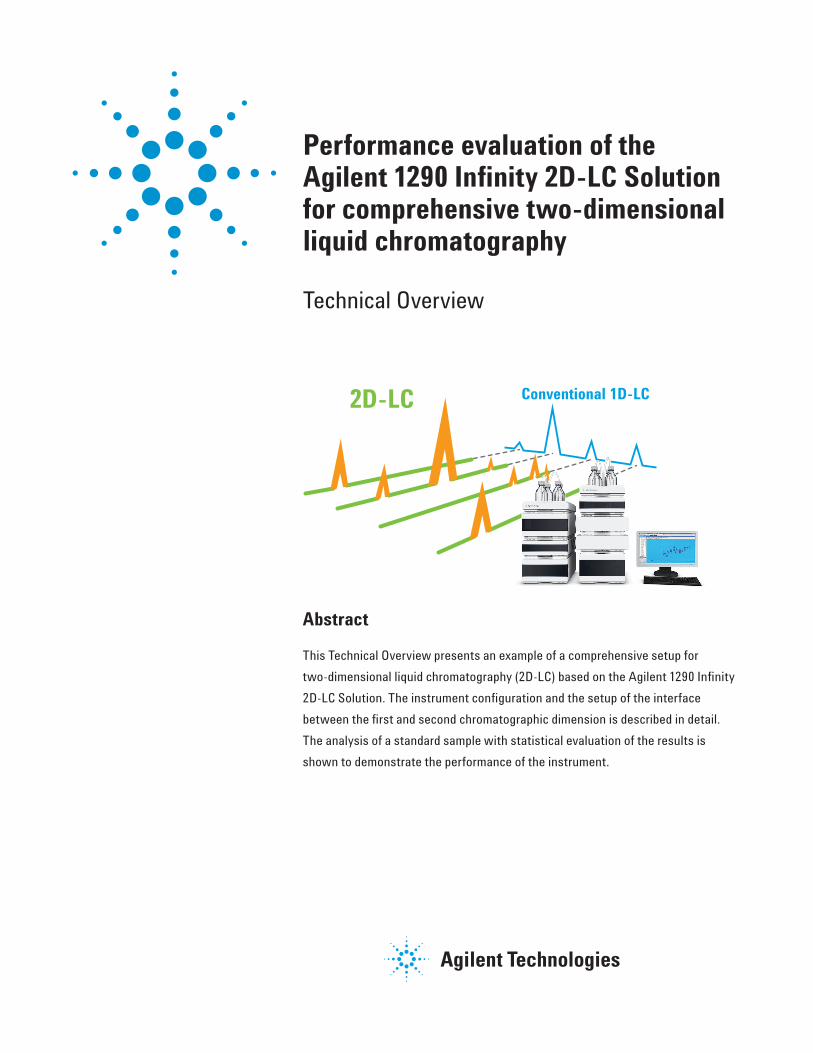
This Technical Overview presents an example of a comprehensive setup for

two‑dimensional liquid chromatography (2D‑LC) based on the Agilent 1290 Infinity

2D‑LC Solution. The instrument configuration and the setup of the interface

between the first and second chromatographic dimension is described in detail.

The analysis of a standard sample with statistical evaluation of the results is

shown to demonstrate the performance of the instrument.

2D-LC Conventional 1D-LC

2

Introduction

The separation of complex samples can be improved by deploying a comprehen‑sive two‑dimensional liquid chroma‑tography (LCxLC) system. In an LCxLC system, typically two pumps and two columns are used and fractions from the separation on the first column (first dimension) are continuously trans‑ferred to a second column (second dimension). This transfer is done by filling two loops alternately controlled by valve switching.

The advantage of LCxLC separation compared to a standard LC separation is the increased peak capacity due to the multiplicative behavior of the peak capacities of the first and second dimension1. This is an idealistic model that is only valid if completely orthogo‑nal separation mechanisms are used for the separation on the columns in the first and second dimension2. This state can be approximated for separa‑tions such as ion exchange in the first and reversed phase separation in the second dimension. In reality, similar selectivities like different reversed phase selectivities are used. In this case, the peak capacity is decreased and can be explained as an accessible triangular area of the two‑dimensional chromatogram used for the separation3. This can be optimized by designing complex gradients for the separation in the second dimension to increase the accessible area used for separation and herewith increasing peak capacity.

To achieve best separation perfor‑mance, a complex gradient was designed for the second dimension by a specialized software tool.

Experimental

EquipmentThe Agilent 1290 Infinity 2D‑LC Solution used for the performance evaluation comprised the following modules:

• Two Agilent 1290 Infinity Pumps (G4220A)

• Agilent 1290 Infinity Autosampler (G4226A) with thermostat (G1330)

• Agilent 1290 Infinity Thermostatted Column Compartment (G1316B) with 2‑position/4‑port duo valve (G4236A) for 2D‑LC

• Agilent 1290 Infinity Diode Array Detector (G4212A) with 60‑mm Agilent Max‑Light flow cell (G4212‑60007)

In this configuration, the first and second dimension pumps are identical. Typically, the second dimension pump must be an Agilent 1290 Infinity pump to deliver fast gradients to the second dimension column. The first dimension pump is flexible and could also be an Agilent 1260/1290 Infinity Quaternary Pump, an Agilent 1260 Infinity Binary Pump or an Agilent 1260 Infinity Capillary Pump.

Software• Agilent OpenLAB CDS ChemStation

Edition, version C.01.03 with 2D‑LC add‑on software

• LCxLC Software for 2D‑LC data analysis from GC Image LLC, Lincoln, NE, USA

ColumnsFirst dimension: Agilent ZORBAX RRHD

Eclipse Plus C18, 150 × 2.1 mm, 1.8 µm

Second dimension: Agilent ZORBAX RRHD

Eclipse Plus Phenyl Hexyl, 50 × 3.0 mm, 1.8 µm

Method

First dimension pumpSolvent A: Acetonitrile +

0.1% formic acid

Solvent B: Water + 0.1% formic acid

Flow rate: 0.1 mL/min

Gradient: 5% B at 0 min 95% B at 30 min 95% B at 40 min

Stop time: 40 min

Post time: 15 min

3

Second dimension pumpSolvent A: Methanol +

0.1% formic acid

Solvent B: Water + 0.1% formic acid

Flow rate: 3 mL/min

Initial gradient: 5% B at 0 min

15% B at 0.5 min 5% B at 0.51 min 5% B at 0.65 min

Gradient modulation: 5% B at 0 min to

50% B at 30 min

15% B at 0.5 min to 95% B at 30 min

5% B at 0.51 min to 50% B at 30 min

5% B at 0.65 min to 50% B at 30 min

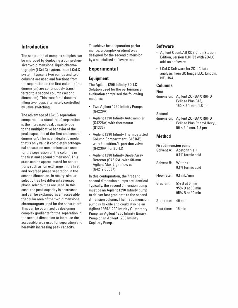
The final second dimension gradient is shown in Figure 1. The user interface for setup of the second dimension gradient is shown and explained in Figure 2.

Figure 1 2D-LC Gradient profile.1st dimension Gradient (red): 0 min 5% B–30 min 95% B, 40 min–95% B. Stop time: 40 min. Post time: 15 min. 2nd dimension Gradient (blue): Initial Gradient: 0 min–5% B, 0.5 min–15% B, 0.51 min–5% B, 0.65 min–5% B. Gradient Modulation: 0 min 5% B to 30 min 50% B, 0.5 min 15% B to 30 min 95% B, 0.51 min 5% to 30 min 50% B, 0.65 min 5% B to 30 min 50% B.

Figure 2 Window for the set-up of the second dimension gradient in a 2D-LC separation.A) Nested table for the set-up of the 2D-LC gradient and gradient shift.B) Table for the set-up of time, and peak-based triggering events to start 2D-LC separation. C) Graphic display of the 2D-LC gradient according to the set-up in the 2D-LC gradient table A and B. The gradient can be changed by drag and drop of the points of the curve in this graphical interface. The changed values are written back to the gradient table.D) Graphical display of a single gradient snip in the second dimension which is repeated by the modulation rate and shifted as given in the gradient table.E) Calculations which help to set-up the 2D-LC separation experiment from currently used LC parameters.

4

Thermostatted column compartment

• First dimension column at left side at 25 °C.

• Second dimension column at right side at 60 °C.

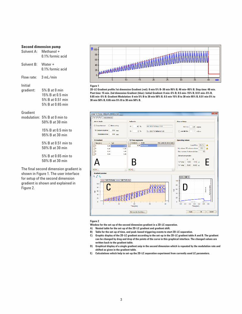
• Two 80 µL loops are connected to the 2‑position/4‑port duo valve and are located at the left side. The valve is switched automatically after each second dimension modulation cycle. The complete plumbing is shown in Figure 3. In this case, the loops are used in a countercurrent manner (the loops are filled and eluted from different sides).

Autosampler• Injection volume: 5 µL

• Sample temperature: 8 °C

• Needle wash: 6 s in methanol

Diode array detector• Wavelength: 260/4 nm,

Ref. 360/16 nm

• Slit: 4 nm

• Data rate: 80 Hz

• Flow cell: 60 mm Max‑Light flow cell

ChemicalsAll solvents used were LC grade. Acetonitrile and methanol were pur‑chased from Merck, Germany. Fresh ultrapure water was obtained from a Milli‑Q Integral system equipped with a 0.22 µm membrane point‑of‑use cartridge (Millipak).

1D-Pump Autosampler

2D-Detector

1D-Column

2D-Column

Waste

Loop_1

Loop_2

12

2D-Pump

Waste

Loop_1

Loop_2

12

1D-Pump Autosampler

2D-Pump 2D-Detector2D-Column

1D-Column

Figure 3 2D-LC with 2-position/4-port duo valve interface configuration, green arrow (&) Fill-direction, red arrow (&) Analyze-direction, (LCxLC, countercurrent).

RRLC Checkout Sample containing ace‑tophenone, propiophenone, butyrophe‑none, valerophenone, hexanophenone, heptanophenone, octanophenone, benzophenone and acetanilide was purchased from Agilent Technologies (p/n 5188‑6529). Gradient Evaluation Mix containing uracil, phenol, methyl paraben, ethyl paraben, propyl paraben, butyl paraben, and heptyl paraben was purchased from Sigma‑Aldrich (catalog no. 48271). Reversed Phase Test Mix containing uracil, phenol, N,N‑Dimethyl‑m‑toluamide and toluene was purchased from Sigma‑Aldrich (catalog no. 47641‑U). Sulfamethazine (Stock solution: 100 µg/mL, catalog no. S6256) and 2‑hydroxy quinoline (Stock solution: 100 µg/mL; catalog no. 270873) were purchased from Sigma‑Aldrich.

SampleThe standards were mixed to a 2D‑LC test sample as following:

• RRLC Checkout Sample: 100 µL

• Gradient Evaluation Mix: 800 µL

• Reversed Phase Test Mix: 200 µL

• Sulfamethazine: 100 µL

• 2‑hydroxy quinoline: 100 µL

5

Results and discussion

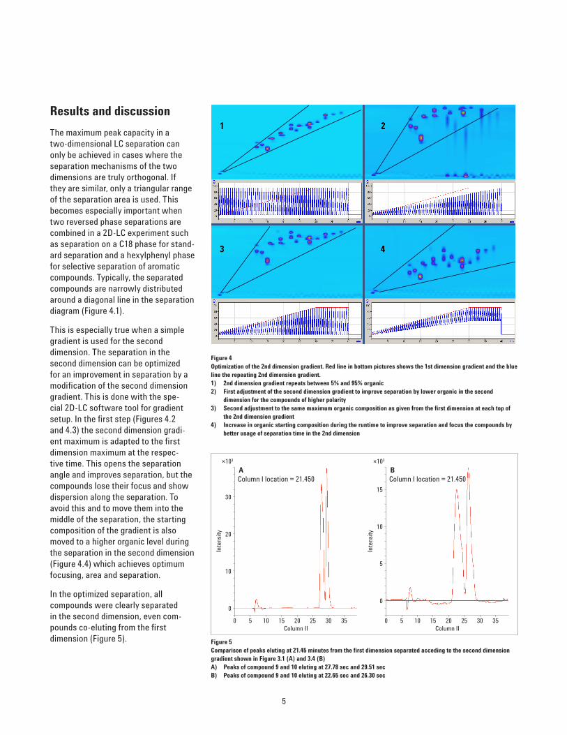
The maximum peak capacity in a two‑dimensional LC separation can only be achieved in cases where the separation mechanisms of the two dimensions are truly orthogonal. If they are similar, only a triangular range of the separation area is used. This becomes especially important when two reversed phase separations are combined in a 2D‑LC experiment such as separation on a C18 phase for stand‑ard separation and a hexylphenyl phase for selective separation of aromatic compounds. Typically, the separated compounds are narrowly distributed around a diagonal line in the separation diagram (Figure 4.1).

This is especially true when a simple gradient is used for the second dimension. The separation in the second dimension can be optimized for an improvement in separation by a modification of the second dimension gradient. This is done with the spe‑cial 2D‑LC software tool for gradient setup. In the first step (Figures 4.2 and 4.3) the second dimension gradi‑ent maximum is adapted to the first dimension maximum at the respec‑tive time. This opens the separation angle and improves separation, but the compounds lose their focus and show dispersion along the separation. To avoid this and to move them into the middle of the separation, the starting composition of the gradient is also moved to a higher organic level during the separation in the second dimension (Figure 4.4) which achieves optimum focusing, area and separation.

In the optimized separation, all compounds were clearly separated in the second dimension, even com‑pounds co‑eluting from the first dimension (Figure 5).

Figure 4 Optimization of the 2nd dimension gradient. Red line in bottom pictures shows the 1st dimension gradient and the blueline the repeating 2nd dimension gradient.1) 2nd dimension gradient repeats between 5% and 95% organic 2) First adjustment of the second dimension gradient to improve separation by lower organic in the second dimension for the compounds of higher polarity 3) Second adjustment to the same maximum organic composition as given from the first dimension at each top of the 2nd dimension gradient 4) Increase in organic starting composition during the runtime to improve separation and focus the compounds by better usage of separation time in the 2nd dimension

Figure 5 Comparison of peaks eluting at 21.45 minutes from the first dimension separated acceding to the second dimension gradient shown in Figure 3.1 (A) and 3.4 (B)A) Peaks of compound 9 and 10 eluting at 27.78 sec and 29.51 secB) Peaks of compound 9 and 10 eluting at 22.65 sec and 26.30 sec

×103

30

20

10

0

0 5 10 15 20Column II

Inte

nsity

25 30 35

Column I location = 21.450A

×103

15

10

5

0

0 5 10 15 20Column II

Inte

nsity

25 30 35

Column I location = 21.450B

6

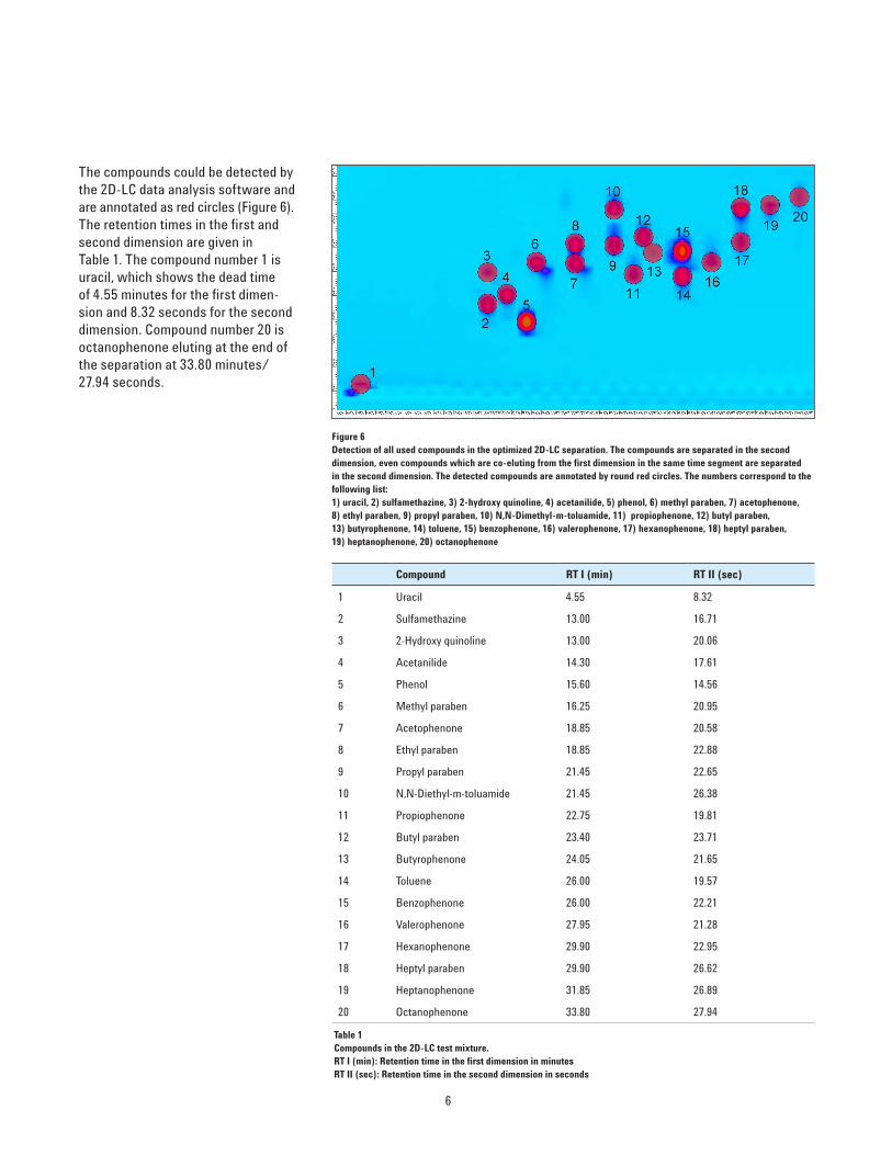
The compounds could be detected by the 2D‑LC data analysis software and are annotated as red circles (Figure 6). The retention times in the first and second dimension are given in Table 1. The compound number 1 is uracil, which shows the dead time of 4.55 minutes for the first dimen‑sion and 8.32 seconds for the second dimension. Compound number 20 is octanophenone eluting at the end of the separation at 33.80 minutes/ 27.94 seconds.

Figure 6 Detection of all used compounds in the optimized 2D-LC separation. The compounds are separated in the second dimension, even compounds which are co-eluting from the first dimension in the same time segment are separated in the second dimension. The detected compounds are annotated by round red circles. The numbers correspond to the following list: 1) uracil, 2) sulfamethazine, 3) 2-hydroxy quinoline, 4) acetanilide, 5) phenol, 6) methyl paraben, 7) acetophenone, 8) ethyl paraben, 9) propyl paraben, 10) N,N-Dimethyl-m-toluamide, 11) propiophenone, 12) butyl paraben, 13) butyrophenone, 14) toluene, 15) benzophenone, 16) valerophenone, 17) hexanophenone, 18) heptyl paraben, 19) heptanophenone, 20) octanophenone

Compound RT I (min) RT II (sec)

1 Uracil 4.55 8.32

2 Sulfamethazine 13.00 16.71

3 2‑Hydroxy quinoline 13.00 20.06

4 Acetanilide 14.30 17.61

5 Phenol 15.60 14.56

6 Methyl paraben 16.25 20.95

7 Acetophenone 18.85 20.58

8 Ethyl paraben 18.85 22.88

9 Propyl paraben 21.45 22.65

10 N,N‑Diethyl‑m‑toluamide 21.45 26.38

11 Propiophenone 22.75 19.81

12 Butyl paraben 23.40 23.71

13 Butyrophenone 24.05 21.65

14 Toluene 26.00 19.57

15 Benzophenone 26.00 22.21

16 Valerophenone 27.95 21.28

17 Hexanophenone 29.90 22.95

18 Heptyl paraben 29.90 26.62

19 Heptanophenone 31.85 26.89

20 Octanophenone 33.80 27.94

Table 1 Compounds in the 2D-LC test mixture.RT I (min): Retention time in the first dimension in minutesRT II (sec): Retention time in the second dimension in seconds

7

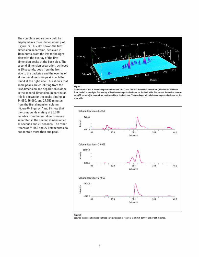
The complete separation could be displayed in a three‑dimensional plot (Figure 7). This plot shows the first dimension separation, achieved in 40 minutes, from the left to the right side with the overlay of the first dimension peaks at the back side. The second dimension separation, achieved in 39 seconds, goes from the front side to the backside and the overlay of all second dimension peaks could be found at the right side. This shows that some peaks are co‑eluting from the first dimension and separation is done in the second dimension. In particular, this is shown for the peaks eluting at 24.050, 26.000, and 27.950 minutes from the first dimension column (Figure 8). Figures 7 and 8 show that the compounds eluting at 26.000 minutes from the first dimension are separated in the second dimension at 19 seconds and 22 seconds. The other traces at 24.050 and 27.950 minutes do not contain more than one peak.

Figure 7 3-dimensional plot of sample separation from the 2D-LC run. The first dimension separation (40 minutes) is shown from the left to the right. The overlay of 1st dimension peaks is shown on the back side. The second dimension separa-tion (39 seconds) is shown from the front side to the backside. The overlay of all 2nd dimension peaks is shown on the right side.

0.0 10.0 20.0 30.0 40.0Column ll

4267.6

_657.1

Inte

nsit

y

0.0 10.0 20.0 30.0 40.0

Column ll

96897.7

_1516.6

Inte

nsit

y

0.0 10.0 20.0 30.0 40.0

Column ll

17904.6

_775.0

Inte

nsit

y

Column location = 24.050

Column location = 26.000

Column location = 27.950

Figure 8 View on the second dimension trace chromatogram in Figure 7 at 24.050, 26.000, and 27.950 minutes.

www.agilent.com/chem/2D-LC

© Agilent Technologies, Inc., 2012Published in USA, April 1, 2012Publication Number 5991‑0138EN

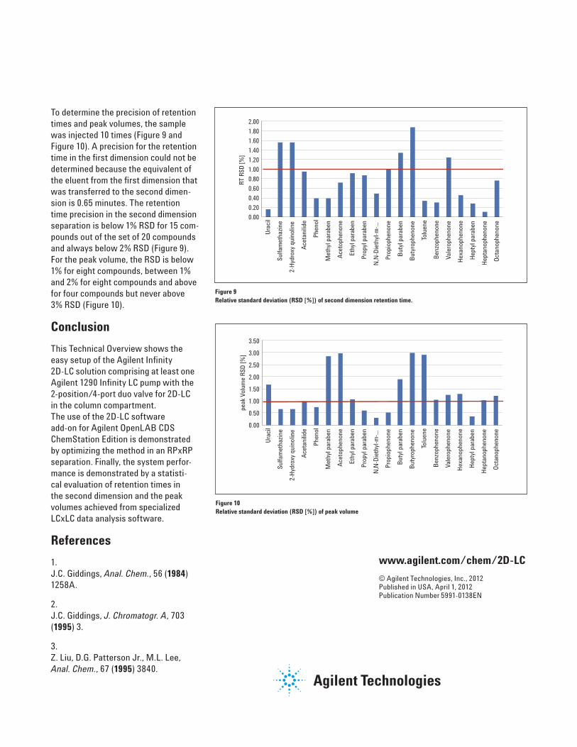
To determine the precision of retention times and peak volumes, the sample was injected 10 times (Figure 9 and Figure 10). A precision for the retention time in the first dimension could not be determined because the equivalent of the eluent from the first dimension that was transferred to the second dimen‑sion is 0.65 minutes. The retention time precision in the second dimension separation is below 1% RSD for 15 com‑pounds out of the set of 20 compounds and always below 2% RSD (Figure 9). For the peak volume, the RSD is below 1% for eight compounds, between 1% and 2% for eight compounds and above for four compounds but never above 3% RSD (Figure 10).

Conclusion

This Technical Overview shows the easy setup of the Agilent Infinity 2D‑LC solution comprising at least one Agilent 1290 Infinity LC pump with the 2‑position/4‑port duo valve for 2D‑LC in the column compartment. The use of the 2D‑LC software add‑on for Agilent OpenLAB CDS ChemStation Edition is demonstrated by optimizing the method in an RPxRP separation. Finally, the system perfor‑mance is demonstrated by a statisti‑cal evaluation of retention times in the second dimension and the peak volumes achieved from specialized LCxLC data analysis software.

References

1. J.C. Giddings, Anal. Chem., 56 (1984) 1258A.

2. J.C. Giddings, J. Chromatogr. A, 703 (1995) 3.

3. Z. Liu, D.G. Patterson Jr., M.L. Lee, Anal. Chem., 67 (1995) 3840.

0.00

0.20

0.40

0.60

0.80

1.00

1.20

1.40

1.60

1.80

2.00

Ura

cil

Sulfa

met

hazi

ne

2-H

ydro

xy q

uino

line

Ace

tani

lide

Phen

ol

Met

hyl p

arab

en

Ace

toph

enon

e

Ethy

l par

aben

Prop

yl p

arab

en

N,N

-Die

thyl

-m-..

.

Prop

ioph

enon

e

But

yl p

arab

en

But

yrop

heno

ne

Tolu

ene

Ben

zoph

enon

e

Vale

roph

enon

e

Hex

anop

heno

ne

Hep

tyl p

arab

en

Hep

tano

phen

one

Oct

anop

heno

ne

RT

RSD

[%]

Figure 9 Relative standard deviation (RSD [%]) of second dimension retention time.

0.00

0.50

1.00

1.50

2.00

2.50

3.00

3.50

peak

Vol

ume

RSD

[%]

Ura

cil

Sulfa

met

hazi

ne

2-H

ydro

xy q

uino

line

Ace

tani

lide

Phen

ol

Met

hyl p

arab

en

Ace

toph

enon

e

Ethy

l par

aben

Prop

yl p

arab

en

N,N

-Die

thyl

-m-..

.

Prop

ioph

enon

e

But

yl p

arab

en

But

yrop

heno

ne

Tolu

ene

Ben

zoph

enon

e

Vale

roph

enon

e

Hex

anop

heno

ne

Hep

tyl p

arab

en

Hep

tano

phen

one

Oct

anop

heno

neFigure 10 Relative standard deviation (RSD [%]) of peak volume