strong particle dispersion by weakly dissipative … particle dispersion by weakly dissipative...

Strong particle dispersion by weaklydissipative random internal wavesOliver Bühler1,†, Nicolas Grisouard1,2 and Miranda Holmes-Cerfon1

1Center for Atmosphere Ocean Science at the Courant Institute of Mathematical Sciences, New YorkUniversity, New York, NY 10012, USA2Department of Environmental Earth System Science, Stanford University, CA 94305, USA

(Received 22 December 2012; revised 25 January 2013; accepted 30 January 2013)

Simple stochastic models and direct nonlinear numerical simulations of three-dimensional internal waves are combined in order to understand the strong horizontalparticle dispersion at second-order in wave amplitude that arises when small-amplitudeinternal waves are exposed to weak dissipation. This is contrasted with the well-knownresults for perfectly inviscid internal waves, in which such dispersion arises only atfourth-order in wave amplitude.

Key words: geophysical and geological flows, mixing and dispersion, waves inrotating fluids

1. Introduction

We report on a somewhat surprising numerical result and on its tentative theoreticalexplanation in connection with our previous studies of particle dispersion by randomwaves in Buhler & Holmes-Cerfon (2009) and Holmes-Cerfon, Buhler & Ferrari(2011). . These studies addressed the fundamental question of how non-breaking small-amplitude gravity waves can contribute to the irreversible quasi-horizontal spreadingof particles along stratification surfaces at very small scales, all with an eye towardsapplications in oceanography. In common with previous studies of similar questions(e.g. Herterich & Hasselmann 1982; Sanderson & Okubo 1988; Weichman & Glazman2000; Balk, Falkovich & Stepanov 2004; Balk 2006), we modelled the linear wavefield as a stationary random process with a power spectrum that is strictly zero atzero frequency, which implies that the linear velocity field cannot by itself give rise toany diffusion in the sense of Taylor (1921) (see § 2 below). The physical motivationfor this assumption was that the frequency of inertia–gravity waves is bounded frombelow by the Coriolis parameter f , which provides a natural non-zero frequency cut-offeverywhere away from the equator.

† Email address for correspondence: [email protected]

J. Fluid Mech. (2013), vol. 719, R4 c© Cambridge University Press 2013 719 R4-1doi:10.1017/jfm.2013.71

mailto:[email protected]

O. Bühler, N. Grisouard and M. Holmes-Cerfon

This implied that particle diffusion could arise only via advection by the wave-induced Lagrangian-mean flow at second-order in wave amplitude. Specifically, if interms of the non-dimensional wave amplitude a� 1 the usual wave energy E0 andthe wave-induced Lagrangian-mean flow are O(a2), then the leading-order diffusivityD, which is quadratic in the advecting velocity, satisfies D = O(a4), i.e. D ∝ E2

0. Ourimplicit presumption was that this result, which was derived assuming unforced andinviscid random waves, would continue to hold approximately for waves that aremaintained in a prescribed stationary state by the combination of weak forcing anddamping, provided only that the damping rate α, say, is reasonably small compared tothe frequencies of the waves.

However, recent direct nonlinear numerical simulations of internal waves in thethree-dimensional rotating Boussinesq system (detailed below in § 4) instead robustlyproduced values for D that were in fact proportional to E0, and not to E2

0 as predictedby theory. This held even for quite weak wave damping and forcing (e.g. the dampingrate is only 2 % of the wave frequency in the typical case displayed in figure 3below). Notably, for small wave amplitude a� 1 the numerically observed O(a2)

particle diffusion was therefore much stronger than the O(a4) diffusivity predicted bythe inviscid theory.

Our subsequent attempt at understanding this surprising result is based on thesequence of simple stochastic models for forced–dissipative waves enumerated in § 3.These simple models allow detailed investigations into the interplay between dampingand diffusion and they show clearly that adding damping is a singular perturbationto the previous inviscid theory: any fixed non-zero amount of damping leads to adiffusivity D that is proportional to the wave energy E0 = O(a2) rather than O(a4)

in the limit of small wave amplitude a� 1. In hindsight this result is perhaps lesssurprising, because the lack of particle diffusion at O(a2) in the inviscid theory reliedcrucially on the exquisite reversibility of linear particle displacements, which is lostif any non-zero amount of damping is introduced. This is the physical basis for thesingular perturbation that we observed, i.e. the dramatic change from weak, O(a4)

particle diffusion to strong, O(a2) particle diffusion induced by the introduction ofweak dissipation.

The paper is organized as follows. The kinematics of Taylor diffusivity aresummarized in § 2 and the simple stochastic models are discussed in § 3. Thenumerical simulations are detailed and compared to predictions from the simplemodels in § 4, which includes an explicit scaling law for D in § 4.3. Concludingcomments are offered in § 5.

2. Kinematics of Taylor diffusivity

The diffusivity of Taylor (1921) as a measure of particle dispersion is the simplestquantity that is relevant to understanding the spreading of passive tracers within a fluidbody. The basic theory applies to the time-evolution of a Cartesian particle coordinateX(t) defined as

dX(t)

dt= u(t), X(0)= 0, ⇒ X(t)=

∫ t

0u(s) ds. (2.1)

Here u(t) is the corresponding Cartesian component of the velocity field, which isclearly the Lagrangian velocity field following the fluid particle. We will assumethroughout that u(t) is a stationary zero-mean random function with covariance

719 R4-2

Strong particle dispersion by weakly dissipative random internal waves

function

C(s)= C(−s)= E[u(t)u(t + s)] such that12

ddt

E[X2] =∫ t

0C(s) ds. (2.2)

Here E denotes probabilistic expectation. Assuming this integral converges as t→∞,this yields the definition of the diffusivity D, i.e.

D=∫ ∞

0C(s) ds= 1

2C(0) such that E[X2] ∼ 2Dt for large t. (2.3)

The second form for D uses the power spectrum C(ω) defined via the Fouriertransform

C(ω)=∫ +∞−∞

e−iωsC(s) ds and C(s)= 12π

∫ +∞−∞

e+iωsC(ω) dω. (2.4)

Finally, if we define the Lagrangian auto-correlation time scale as

τ =∫ ∞

0

C(s)

C(0)ds= 1

2C(0)C(0)

= D

E[u2] then D= E[u2] τ. (2.5)

At fixed E[u2] the diffusivity D is simply proportional to τ .

3. Simple stochastic models for forced–dissipative velocity fields

We consider three simple, exactly solvable linear stochastic differentialequation (SDE) models for the forced–dissipative evolution of a wave-like Lagrangianvelocity field u. Common to these models is that there is a one-parameter family ofpossible combinations of forcing and dissipation parameters that maintain the samevariance E[u2], but change the time scale τ and therefore the diffusivity D. This is thekey step in order to understand the direct numerical simulations of forced–dissipativewaves that follow in § 4. The three models are gradually increasing in complexity andrelevance, and the third model, which encompasses the other two in suitable limits,provides the best theoretical guidance for understanding the full internal wave problem.

3.1. Ornstein–Uhlenbeck processThe Ornstein–Uhlenbeck (OU) process for u(t) is defined by the SDE

du

dt+ αu= βξ with E[ξ ] = 0 and E[ξ(t1)ξ(t2)] = δ(t1 − t2). (3.1)

Here the constant parameters α > 0 and β quantify the damping rate and forcingstrength, respectively. Strictly speaking, the white-noise forcing ξ(t) is not a functionbut a distribution, and it merely serves as a convenient shorthand for the increment ofthe Wiener process dW = ξ dt that necessarily appears in the general theory of SDEs(e.g. Gardiner 1997). This is sufficient for the simple additive noise examples we arestudying here, but would have to be reconsidered in the case of multiplicative noise,where β depends on u. The OU process has a stationary distribution with (see theAppendix)

C(ω)= β2

ω2 + α2and C(s)= β2

2αe−α|s|. (3.2)

719 R4-3


The variance is E[u2] = C(0)= β2/2α and hence for the OU process constant varianceof u implies the one-parameter family β2 ∝ α. It then follows from (2.3) and (2.5) that

Ornstein–Uhlenbeck: D= β2

2α2=(β2

2α

)1α⇒ τ = 1

α. (3.3)

This illustrates the well-known fact that the OU auto-correlation time scale τ is equalto the damping time scale 1/α. In particular, as the damping rate goes to zero thediffusivity at fixed variance goes to infinity.

As a model for forced–dissipative linear waves the OU process neatly illustrates thegeneral point that D is not fixed, but depends on the modelling choice for the dampingrate α. However, the absence of any intrinsic wave dynamics in the evolution equationfor u(t) rather limits the direct utility of the OU process for the problem at hand. Thetwo following models improve on this point.

3.2. Linear harmonic oscillatorThe linear harmonic oscillator (LHO) is defined by the second-order equation

d2u

dt2+ α du

dt+ ω2

0u= βω0ξ, (3.4)

where the new parameter ω0 > 0 is the natural frequency of the undamped oscillatorand β measures the white-noise forcing strength as before (the factor ω0 has beeninserted to keep the units of β the same as in (3.1)). Damped oscillatory motion occursfor values of α below the threshold α = 2ω0. The case of weak damping, in whichα � ω0, is perhaps the most relevant in practice, but we can actually calculate allour results here without restriction on the size of α. In particular, we obtain (see theAppendix)

C(ω)= β2ω20

(ω2 − ω20)

2+α2ω2and D= β2

2ω20

. (3.5)

Remarkably, the diffusivity is independent of α in this expression. However, what isrelevant for us here is the diffusivity at fixed variance of u, and for this we need thecovariance function, which for α < 2ω0 is

C(s)= β2

2αe−α|s|/2

{cos (γ s)+ α

2γsin (γ |s|)

}with γ =

√∣∣∣∣ω20 −

α2

4

∣∣∣∣. (3.6)

In the complementary case α > 2ω0 the functions (cos, sin) are replaced by(cosh, sinh), respectively. Either way the variance is again E[u2] = C(0) = β2/2α andwe obtain

Linear harmonic oscillator: D= β2

2ω20

=(β2

2α

)α

ω20

⇒ τ = α

ω20

. (3.7)

This remarkable formula shows that at fixed ω0 and E[u2] the diffusivity isproportional to the damping rate α and accordingly goes to zero as α→ 0. Thislimit is consistent with the earlier argument that a freely evolving linear wave withnon-zero frequency (i.e. ω0 > 0) has D = 0. However, we also see that any amountof damping, no matter how small, breaks this condition and delivers a non-zero Daccording to (3.7).

719 R4-4


Now, as a model for a linear wave velocity u the LHO improves on the OU processby introducing a natural wave frequency ω0. Still, in a fluid-dynamical model onewould add random forcing in the equation for du/dt, whereas in the LHO equation theforcing acts on d2u/dt2 instead. This leads us to the third model.

3.3. Inertial oscillationsThe third model is based on the inertial oscillations of a horizontally homogeneoussingle fluid layer relative to a state of rest in a rotating frame of reference withCoriolis parameter f , say. The horizontal velocity vector u = (u, v) and the governingSDEs are

du

dt+ αu− fv = βξ1 and

dvdt+ αv + fu= βξ2. (3.8)

Here ξ1(t) and ξ2(t) are independent versions of white noise. In the stationary regimeu and v are identically distributed and for their common power spectrum and auto-correlation function we obtain (see the Appendix)

C(ω)= 12

(β2

(ω + f )2+α2+ β2

(ω − f )2+α2

)and C(s)= β2

2αcos(fs)e−α|s|. (3.9)

Comparing (3.9) with (3.2) it is clear that this is the natural generalization of the OUprocess to the case of a natural wave frequency f . Once more the variance of u isβ2/2α and the diffusivity is

Inertial oscillations: D= 12

β2

f 2 + α2=(β2

2α

)α

f 2 + α2⇒ τ = α

f 2 + α2. (3.10)

The time scale of this process interpolates between the former two: for small α itapproximates the LHO with τ ∝ α whilst for large α it approximates the OU processwith τ ∝ 1/α. As will be shown below, this is essentially what we observe for theTaylor diffusivity in direct numerical simulations of wave-induced particle dispersiondue to forced–dissipative internal gravity waves.

4. Direct numerical simulations

We describe direct numerical simulations of small-amplitude internal waves using afully nonlinear three-dimensional numerical model for the rotating Boussinesq systemwith linear damping and white-noise wave forcing in time.

4.1. Numerical set-upWe use a modification of the pseudo-spectral model of Winters, MacKinnon & Mills(2004), which solves

ut + (u ·∇)u+ f z× u+∇P− bz=+D6u− αquq + F, (4.1a)

bt + (u ·∇)b+ N2w=+D6b− αqbq, and ∇ · u= 0. (4.1b)

Here u = (u, v,w) is the velocity vector, f = 10−4 s−1 is the Coriolis parameter, z isthe vertical unit vector, P is the scaled pressure fluctuation, b is the buoyancy, andN = 10−3 s−1 is the constant buoyancy frequency. The dissipation operator D6 is

D6 =+(ν6H (∂

2x + ∂2

y )3+ν6z∂

6z

), (4.2)

719 R4-5


where ν6H and ν6z are horizontal and vertical dissipation coefficients. The additionaldamping related to αq is discussed below (4.6). Our numerical domain is atriply periodic rectangular box with horizontally square cross-section of side lengthL = 1 km and vertical height H = δL = 100 m, so the aspect ratio δ = f /N = 1/10.The numerical grid is flattened in the vertical and the domain is discretized withn= 96 points in all three directions. We choose ν6z = δ6ν6H .

All fields X are expanded into discrete Fourier series of the form

X(x, y, z, t)=∑k,l,m

Xklm(t) exp[i (kx+ ly+ mz)], (4.3)

where (k, l, δm) can take values from the discrete sets {−n/2+ 1, . . . , n/2} × 2π/L.The reality condition X∗−(klm) = Xklm is enforced numerically by evolving the fields fork > 0 only and then extending the results to k < 0 by complex conjugation.

The wave forcing F based on white noise in time is designed to have no effect onthe linear potential vorticity (PV) of the system, which is q = z · (∇ × u) + f bz/N2.Otherwise the forcing would produce an unwanted balanced, PV-controlled flow at thesame order as the waves, which would dominate the particle advection. This requiresthat z · (∇ × F) = 0, and we also find it convenient to enforce ∇ · F = 0 becauseany divergent part of F is absorbed by the pressure gradient. In spectral space this isachieved by

Fklm(t)= 1kHK

−km−lmk2

H

ξ(t) and F∗−(klm)(t)= Fklm(t), (4.4)

where K =√

k2H + m2. Here ξ = ξR + iξI is a complex normal random variable

(independent from time step to time step) with independent real and imaginary parts ξR

and ξI such that at each numerical time step with step size 1t

E[ξR,I

]= 0, E [ξRξI]= 0 and E[ξ 2

R,I

]= 2αkHmEklm/1t. (4.5)

Here αkHm = ν6Hk6H + ν6zm6, 1t = 100 s the numerical time step and Eklm is a spectral

energy density that is related to the expected energy by

E0 = 12

E[

u2 + v2 + w2 + b2

N2

]=∑k,l,m

Eklm. (4.6)

For time stepping a third-order Adams–Bashforth (AB3) scheme is used for all termsexcept the random force, which is instead advanced using forward Euler. To minimizealiasing whilst maintaining numerical accuracy, 1/9 of the wavenumbers are truncatedfollowing Patterson & Orszag (1971).

There is one important caveat that we need to mention. Although F as defined doesnot project onto the linear PV, in the presence of internal waves it does project on theexact nonlinear PV defined by Q=∇(N2z+b) ·(∇×u+ f z) via the O(a2) forcing term∇b · (∇ × F), which will produce an unwanted balanced flow at O(a2). Although thisis much smaller than the O(a) waves, this nearly steady balanced flow can still leadto significant particle advection and hence we have found it necessary to continuouslydamp the balanced flow. To this end we diagnose at each time step the linear balanced

719 R4-6


–0.2 –0.1 0 0.1 0.2

100

10000z

(m)

y (m)x (m)

500

0

500

1000

1

0

–1

m (

m–1

)

l (m–1) k (m–1)

2

–2

0.20.2

–0.2 –0.2

00

6

5

4

3

2

1

(× 104)(a) (b)

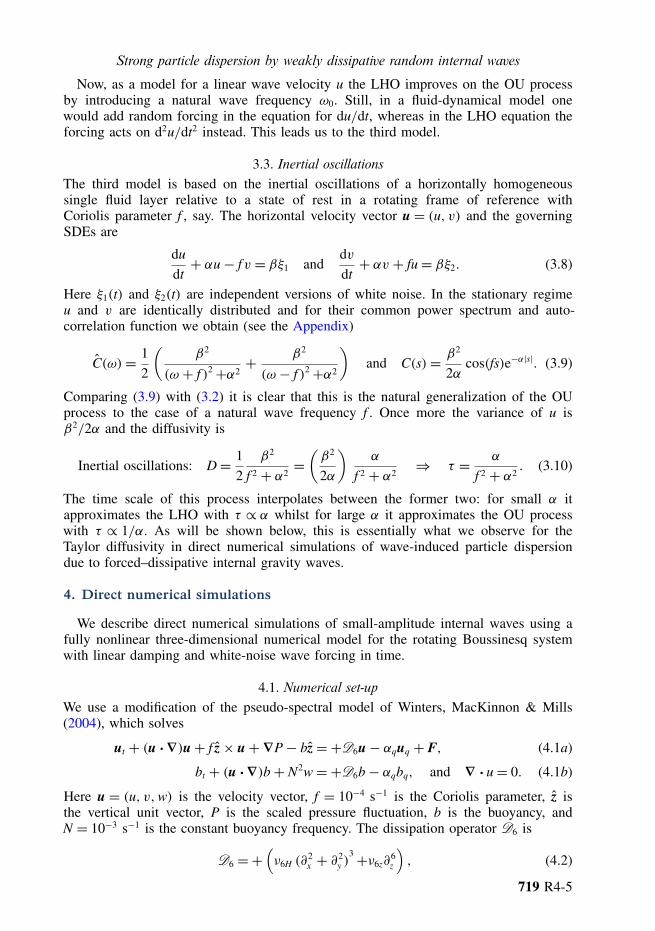
FIGURE 1. Snapshots of the scaled horizontal divergence (ux + vy)/f = −wz/f for E0 =2 × 10−9 m2 s−2 and α0/ω0 = 2.4 × 10−3 in (a) physical space and (b) spectral space (theabsolute value of the Fourier transform is shown). The non-dimensional wave amplitude is∼10 % in this example.

flow (uq, bq) from the instantaneous q via a quasi-geostrophic stream function ψ , i.e.

ψxx + ψyy + f 2

N2ψzz = q and uq =−ψy, vq = ψx, wq = 0, bq = fψz. (4.7)

This linear balanced flow is then damped with decay rate αq = 1/250 s−1.

4.2. Results for particle dispersion and diffusivity D

All numerical experiments are executed using the same functional form of the waveenergy spectrum localized at a central frequency ω0 and a scaled wavenumber Ks0 via

Eklm = (E0/nF)× 1−1ω/26ω−ω06+1ω/2 × 1−1Ks/26Ks−Ks06+1Ks/2. (4.8)

Here nF is the number of modes for which Eklm 6= 0, the indicator function 1X is unityif X is true and zero otherwise and

Ks(kH,m)= L√

k2H + δ2m2

πnand ω(kH,m)=

√k2

HN2 + m2f 2

K(4.9)

are the scaled total wavenumber and the positive inertia–gravity wave frequency,respectively. We use ω0/f = 2.06, 1ω/f = 2.01, Ks0 = 0.56 and 1Ks = 0.08. Hencethe central wave has horizontal and vertical wavelengths of ∼43 and 8 m, respectively,and its frequency is near-inertial, which makes the simple model § 3.3 relevant withω0 replacing f . Figure 1 shows snapshots of the wave field in both physical andspectral space, where the signature of the forcing in spectral space is clearly seen. Thedamping rate αkHm does not vary much over the range of excited wavenumbers in (4.8)and we will simply denote its average over these wavenumbers by α0.

We seed the fluid with 64 Lagrangian particles in a regular 4 × 4 × 4 pattern (seefigure 2). To maximize the distance between particles, a rudimentary staggering of

719 R4-7


1000

1000

500

0

500

1000

x (m)x (m)y (m)

y (m)

z (m

)

39.5

9493

9291 94

9698

100

(a) (b)

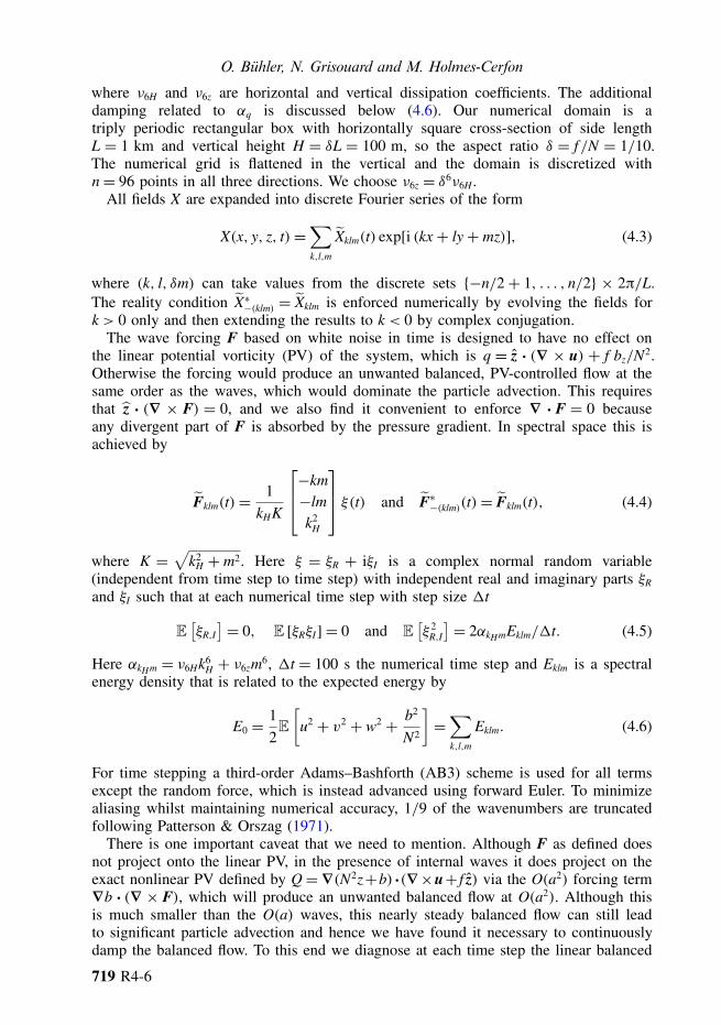
FIGURE 2. Three-dimensional view of the particle trajectories in the example from figure 1.(a) All particle trajectories, enlarged 10 times for clarity. Particles are colour-coded as a functionof their initial altitude: darker means lower. (b) A single particle trajectory in actual size withcolour indicating time from t = 0 (dark) to t = 600 days (light). The trajectory is dominated byinertial circles superimposed on a weak random walk.

t (days)

(a)

R2

(m2 )

50

100

150

200

0 100 200 300 400 500t (days)

(b)

50

100

150

200

0 100 200 300 400 500

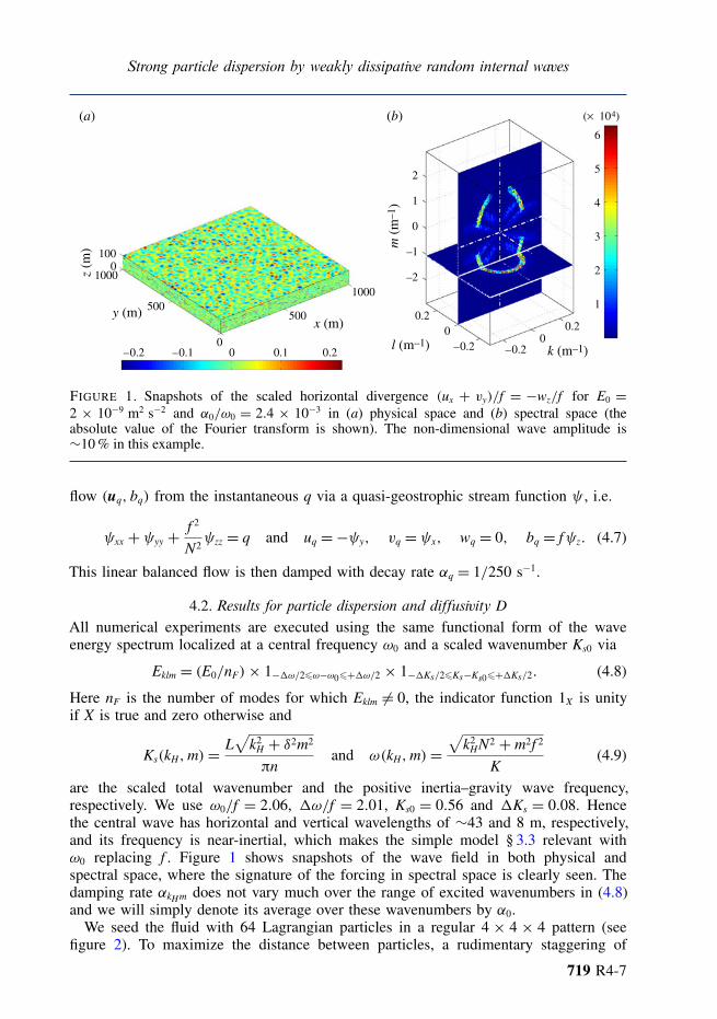
FIGURE 3. Statistics on particle displacements for α0/ω0 = 2.0×10−2 and (a) E0 = 10−9 m2 s−2

and (b) E0 = 5 × 10−10 m2 s−2. Shading: area centred around the median position where 50 %of the particles are found. Black line: estimated R2, which equals 4Dt under Taylor diffusion. Acomparison shows very clearly that the slope 4D∝ E0.

the initial horizontal positions across the vertical direction is implemented. Finally,contrary to what is described in Winters et al. (2004), the velocity at each particleposition is interpolated from the Eulerian velocities at the neighbouring grid points,without communication between processors in parallel configurations, and an AB3scheme is used to advect the particles.

We assume that the particles are experiencing horizontal Taylor diffusion if

R2 = E[R2

i

]= 4Dt, where Ri =√(xi − x0i)

2+ (yi − y0i)2 (4.10)

is the horizontal displacement of the ith particle. The expectation is estimated by anaverage over all particles and over eleven independent runs. Figure 3 shows R2 as afunction of time in two cases with weak damping, indicating that R2 is proportional totime and also that D∝ E0 = O(a2) instead of the inviscid prediction D∝ E2

0 = O(a4).

4.3. A diffusivity scaling law for very weak dampingLetting α0/ω0 → 0 at fixed amplitude a presumably recovers the O(a4) diffusivityof the inviscid theory. Now, for very weak damping with α0/ω0 comparableto O(a2) we expect this inviscid O(a4) diffusivity to be comparable to theforced–dissipative O(a2) diffusivity. In this regime we may use the theoretical

719 R4-8


Linear regression

(× 1010) (× 10–6)

2

4

6

8

10

0 1000 2000 3000 4000

0.5

1.0

1.5

0 400

0.5

1.0

1.5

2.0

2.5

0 1 2 3 4 5

(a) (b)

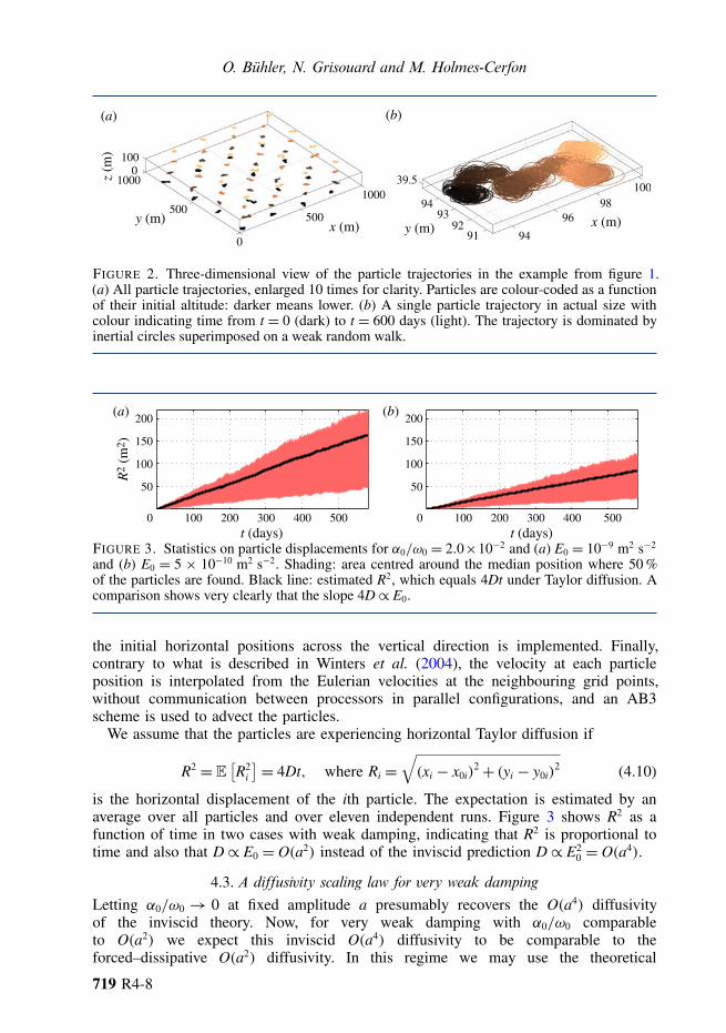
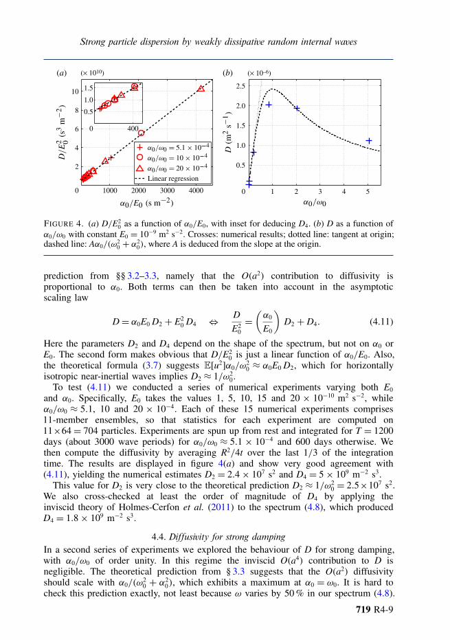
FIGURE 4. (a) D/E20 as a function of α0/E0, with inset for deducing D4. (b) D as a function of

α0/ω0 with constant E0 = 10−9 m2 s−2. Crosses: numerical results; dotted line: tangent at origin;dashed line: Aα0/(ω

20 + α2

0), where A is deduced from the slope at the origin.

prediction from §§ 3.2–3.3, namely that the O(a2) contribution to diffusivity isproportional to α0. Both terms can then be taken into account in the asymptoticscaling law

D= α0E0 D2 + E20 D4 ⇔ D

E20

=(α0

E0

)D2 + D4. (4.11)

Here the parameters D2 and D4 depend on the shape of the spectrum, but not on α0 orE0. The second form makes obvious that D/E2

0 is just a linear function of α0/E0. Also,the theoretical formula (3.7) suggests E[u2]α0/ω

20 ≈ α0E0 D2, which for horizontally

isotropic near-inertial waves implies D2 ≈ 1/ω20.

To test (4.11) we conducted a series of numerical experiments varying both E0

and α0. Specifically, E0 takes the values 1, 5, 10, 15 and 20 × 10−10 m2 s−2, whileα0/ω0 ≈ 5.1, 10 and 20 × 10−4. Each of these 15 numerical experiments comprises11-member ensembles, so that statistics for each experiment are computed on11×64= 704 particles. Experiments are spun up from rest and integrated for T = 1200days (about 3000 wave periods) for α0/ω0 ≈ 5.1 × 10−4 and 600 days otherwise. Wethen compute the diffusivity by averaging R2/4t over the last 1/3 of the integrationtime. The results are displayed in figure 4(a) and show very good agreement with(4.11), yielding the numerical estimates D2 = 2.4× 107 s2 and D4 = 5× 109 m−2 s3.

This value for D2 is very close to the theoretical prediction D2 ≈ 1/ω20 = 2.5×107 s2.

We also cross-checked at least the order of magnitude of D4 by applying theinviscid theory of Holmes-Cerfon et al. (2011) to the spectrum (4.8), which producedD4 = 1.8× 109 m−2 s3.

4.4. Diffusivity for strong dampingIn a second series of experiments we explored the behaviour of D for strong damping,with α0/ω0 of order unity. In this regime the inviscid O(a4) contribution to D isnegligible. The theoretical prediction from § 3.3 suggests that the O(a2) diffusivityshould scale with α0/(ω

20 + α2

0), which exhibits a maximum at α0 = ω0. It is hard tocheck this prediction exactly, not least because ω varies by 50 % in our spectrum (4.8).

719 R4-9


Still, investigating this by a series of 600 day runs in which E0 is kept constant at10−9 m2 s−2 whilst α0/ω0 is varied from 5.1 × 10−4 to 5.1 led to the encouragingresults shown in figure 4(b).

5. Concluding comments

Our direct numerical wave simulations turned out to be compatible with the simplestochastic model based on (2.5) and (3.10) for the O(a2) horizontal diffusivity due tointernal waves with frequency ω0 and damping rate α0:

D= E[u2] τ = E[u2] α0

ω20 + α2

0

. (5.1)

For weak damping the relevant auto-correlation time scale is τ = α0/ω20. Of course,

a practical application of simple stochastic models such as (5.1) first requires anunderstanding of the real wave damping mechanisms, which are rarely linear and mayinvolve wave breaking, and also a justification of the forcing model based on whitenoise in time. This is never an easy task in macroscopic fluid dynamics. Still, we planto consider these ideas for the internal wave spectrum in the ocean, where estimatesfor the highly intermittent decay rate range from a few days to several months (e.g.Munk 1981).

There is another physical shortcoming of our simple model, namely that once weallow for realistic wave dissipation we must also allow for the concomitant generationof PV that inevitably arises at O(a2) in momentum-conserving physical systems (e.g,Buhler 2000). In our numerical model the PV was strongly damped by design, sothis process was eliminated. We hope to address in the near future the interestingfundamental problem of particle dispersion due to a self-consistent ensemble of weaklydissipative waves together with their concomitant wave-induced balanced flows.

Acknowledgements

We thank K. Winters for his kind assistance with the numerical model. Financialsupport for O.B. and N.G. under the United States National Science Foundation grantsDMS-1009213 and OCE-1024180 is gratefully acknowledged.

Appendix. Derivation of power spectra in § 3

By definition, the power spectrum C(ω) of a real-valued stationary zero-meanrandom process u(t) is the Fourier transform of C(s) = E[u(t)u(t + s)] with respectto the time lag s. Using (2.4) this can be written in terms of the distributional Fouriertransform u(ω)= u∗(−ω) as

C(ω)= 12π

∫ +∞−∞

ei(ω−ω′)t E[u(ω)u∗(ω′)] dω′ = 12π

∫ +∞−∞

E[u(ω)u∗(ω′)] dω′. (A 1)

The second form uses E[u(ω)u∗(ω′)] = 0 if ω 6= ω′. The distribution u(ω) is easilyexpressed in terms of the distribution ξ (ω) = ξ ∗(−ω) by taking the Fourier transformof the governing SDE; it is this step that ensures that u follows the invariant measureof the SDE. For example, for the OU process this yields u = βξ/(iω + α). Evaluating(A 1) is then straightforward after noting the spectral equivalent of the second of (3.1):

E[ξ(t1)ξ(t2)] = δ(t1 − t2) ⇔ E[ξ (ω)ξ ∗(ω′)] = 2π δ(ω − ω′). (A 2)

719 R4-10


This immediately yields C(ω) and hence the corresponding functions C(s) in§§ 3.1–3.2.

The two-variable case in § 3.3 is best analysed using the complex variable z= u+ ivsuch that (3.8) become the complex SDE dz/dt+ αz+ ifz= β(ξ1+ iξ2). The equivalentof (A 1) for the transform Q(ω) of the complex auto-correlation function

Q(s)= E[z∗(t)z(t + s)] is then Q(ω)= 12π

∫ +∞−∞

E[z(ω)z∗(ω′)] dω′. (A 3)

Using E[ξi(ω)ξ∗j (ω

′)] = 2π δijδ(ω − ω′) this is evaluated as

Q(ω)= 2β2

(ω + f )2+α2and Q(s)= β

2

αe−ifse−α|s|. (A 4)

Note that Q∗(−s)= Q(s). From (A 3) it then follows that

Q(s)= E[u(t)u(t + s)] + E[v(t)v(t + s)] + i (E[u(t)v(t + s)] − E[u(t)v(t − s)]) (A 5)

after using stationarity for the final term. In the present case u(t) and v(t) areidentically distributed (though not independent) and therefore

C(s)= E[u(t)u(t + s)] = 12

Re Q(s)= β2

2αcos(fs)e−α|s|. (A 6)

Analogously, E[u(t)v(t + s)] = Im Q(s)/2 = −(β2/2α) sin(fs)e−α|s|. Finally, (A 6)implies C(ω)= (Q(ω)+ Q∗(−ω))/4, so with real Q(ω) one can also note the shortcutsD= Q(0)/4, E[u2] = Q(0)/2, and τ = Q(0)/2Q(0).

References

BALK, A. M. 2006 Wave turbulent diffusion due to the Doppler shift. J. Stat. Mech. P08018.BALK, A. M., FALKOVICH, G. & STEPANOV, M. G. 2004 Growth of density inhomogeneities in a

flow of wave turbulence. Phys. Rev. Lett. 92, 244504.BUHLER, O. 2000 On the vorticity transport due to dissipating or breaking waves in shallow-water

flow. J. Fluid Mech. 407, 235–263.BUHLER, O. & HOLMES-CERFON, M. 2009 Particle dispersion by random waves in rotating shallow

water. J. Fluid Mech. 638, 5–26.GARDINER, C. W. 1997 Handbook of Stochastic Methods. Springer.HERTERICH, K. & HASSELMANN, K. 1982 The horizontal diffusion of tracers by surface waves.

J. Phys. Oceanogr. 12, 704–712.HOLMES-CERFON, M., BUHLER, O. & FERRARI, R. 2011 Particle dispersion by random waves in

the rotating Boussinesq system. J. Fluid Mech. 670, 150–175.MUNK, W. 1981 Internal waves and small-scale processes. In Evolution of Phys. Oceanography (ed.

B. Warren & C. Wunsch). pp. 264–291. MIT Press.PATTERSON, G. S. & ORSZAG, S. A. 1971 Spectral calculations of isotropic turbulence: efficient

removal of aliasing interactions. Phys. Fluids 14 (11), 2538–2541.SANDERSON, B. G. & OKUBO, A. 1988 Diffusion by internal waves. J. Geophys. Res. 93,

3570–3582.TAYLOR, G. I. 1921 Diffusion by continuous movements. Proc. Lond. Math. Soc. 20, 196–212.WEICHMAN, P. & GLAZMAN, R. 2000 Passive scalar transport by travelling wave fields. J. Fluid

Mech. 420, 147–200.WINTERS, K. B., MACKINNON, J. A. & MILLS, B. 2004 A spectral model for process studies of

rotating, density-stratified flows. J. Atmos. Ocean. Technol. 21 (1), 69–94.

719 R4-11

strong particle dispersion by weakly dissipative … particle dispersion by weakly dissipative...

Documents