modelling and simulation of stepup and stepdown … and simulation of stepup and stepdown...

Modelling and Simulation of Step-Up and

Step-Down Transformers

MARIUS-CONSTANTIN POPESCU1 NIKOS MASTORAKIS

2

1Faculty of Electromechanical and Environmental Engineering, University of Craiova

ROMANIA 2Technical University of Sofia

BULGARIA

[email protected] [email protected]

Abstract: The current and power (active and reactive parts) at the terminals of the step-down

transformer are positive if the transit is in line busbar to charge. The study of the dynamic behavior of

the system developed in the later, will use numerical simulations and the calculation of eigen values.

Key-Words: Step-up and step-down transformers, Power model and current.

1 Introduction The initial state of the system will be a steady one.

For this, we must give the value of state variables

of system and also the interface variables between

different blocks of the model. The value of some of

these variables can be chosen arbitrarily (within the

limits of validity of models), the value of others

may be inferred from the first through the use of

relationships between variables in steady state. The

definition of an initial state is to choose a set of

variables of the system so we can assign a value

independently and that the set of all other variables

in the system can be inferred. We will describe later

in this section the overall system initialization, that

is to say the choice of independent variables and

calculating the interface variable models of areas

and lines. Initialization within each component

models will be presented at the same time as the

description thereof. In steady state, the frequency is

the same everywhere in the system. We assume

here that the initial state, this frequency is the

nominal frequency. We take as a basic option that

the active production and voltage generators are

given, and also the active and reactive power of the

charges for voltage and nominal frequency. In this

context, in general, the active power balance is not

checked. Therefore, the active production of one of

the generators will not be fixed (node beam). In this

node, a reference phase is chosen. Compared to the

conventional approach to charge flow, it is

necessary to make the following remarks [1],[3],[7]

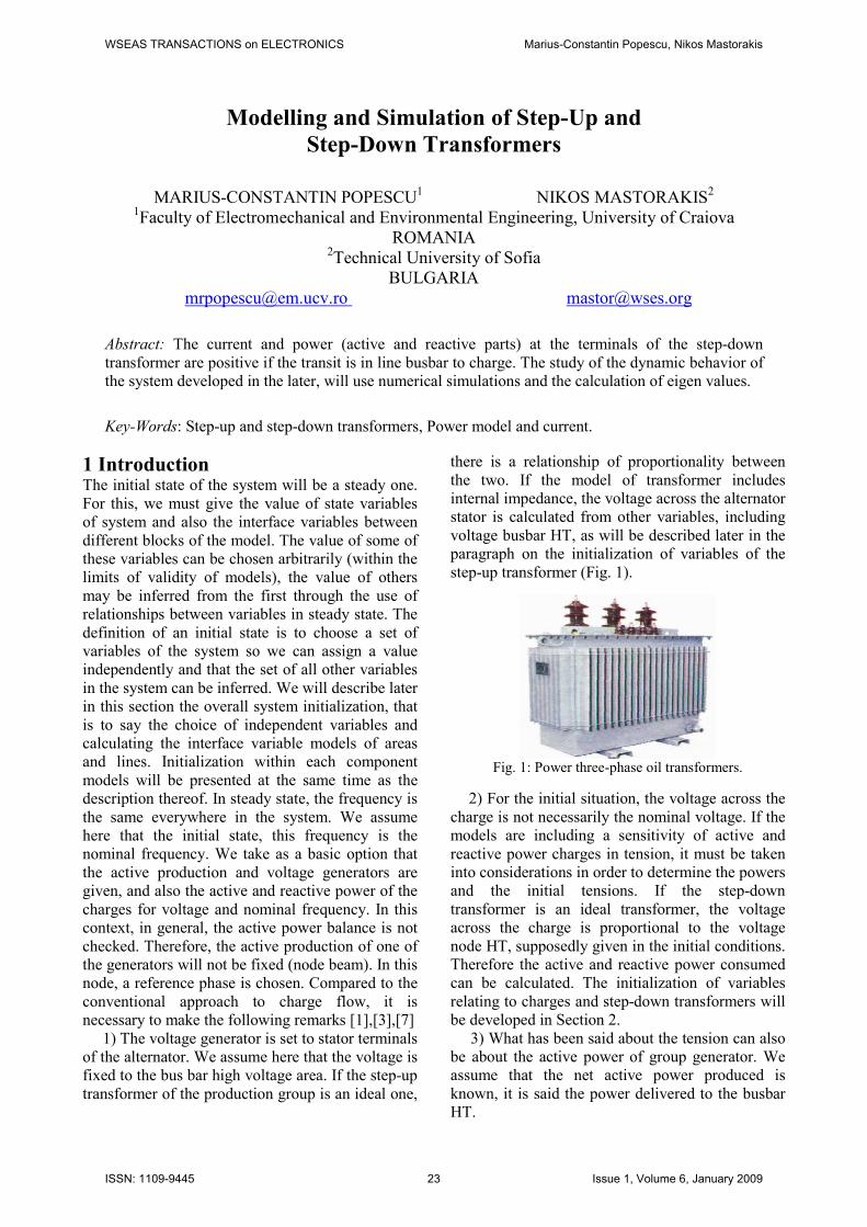
1) The voltage generator is set to stator terminals

of the alternator. We assume here that the voltage is

fixed to the bus bar high voltage area. If the step-up

transformer of the production group is an ideal one,

there is a relationship of proportionality between

the two. If the model of transformer includes

internal impedance, the voltage across the alternator

stator is calculated from other variables, including

voltage busbar HT, as will be described later in the

paragraph on the initialization of variables of the

step-up transformer (Fig. 1).

Fig. 1: Power three-phase oil transformers.

2) For the initial situation, the voltage across the

charge is not necessarily the nominal voltage. If the

models are including a sensitivity of active and

reactive power charges in tension, it must be taken

into considerations in order to determine the powers

and the initial tensions. If the step-down

transformer is an ideal transformer, the voltage

across the charge is proportional to the voltage

node HT, supposedly given in the initial conditions.

Therefore the active and reactive power consumed

can be calculated. The initialization of variables

relating to charges and step-down transformers will

be developed in Section 2.

3) What has been said about the tension can also

be about the active power of group generator. We

assume that the net active power produced is

known, it is said the power delivered to the busbar

HT.

WSEAS TRANSACTIONS on ELECTRONICS Marius-Constantin Popescu, Nikos Mastorakis

ISSN: 1109-9445 23 Issue 1, Volume 6, January 2009

2 Basic Model of a Transformer

without Losses As part of the study presented here, we can

reasonably suppose that the magnetizing current of

the transformers and the losses by Joule effect in

the windings have a negligible influence [11], [16].

Therefore, the model of the transformer is reduced

to a series reactance X and an ideal transformer of

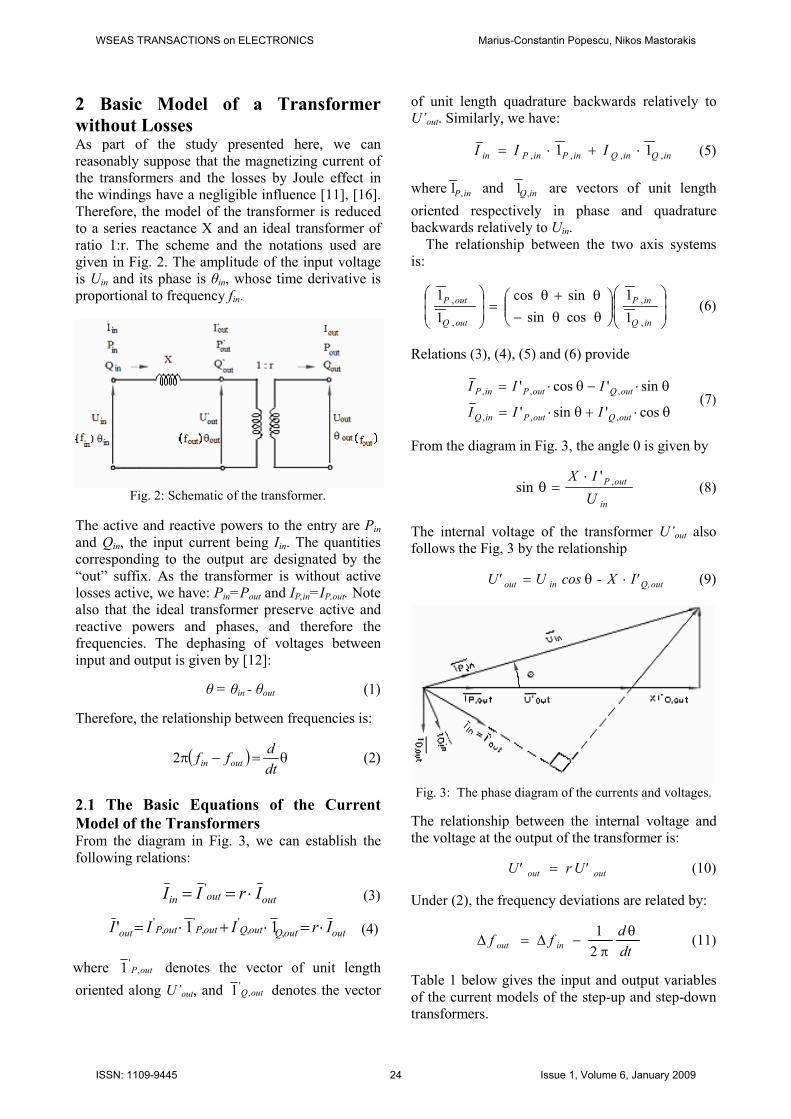
ratio 1:r. The scheme and the notations used are

given in Fig. 2. The amplitude of the input voltage

is Uin and its phase is θin, whose time derivative is

proportional to frequency fin.

Fig. 2: Schematic of the transformer.

The active and reactive powers to the entry are Pin

and Qin, the input current being Iin. The quantities

corresponding to the output are designated by the

“out” suffix. As the transformer is without active

losses active, we have: Pin=Pout and IP,in=IP,out. Note

also that the ideal transformer preserve active and

reactive powers and phases, and therefore the

frequencies. The dephasing of voltages between

input and output is given by [12]:

θ = θin - θout (1)

Therefore, the relationship between frequencies is:

( ) θ=−πdt

dff outin2 (2)

2.1 The Basic Equations of the Current

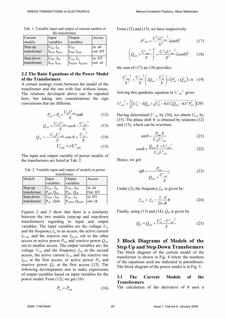
Model of the Transformers From the diagram in Fig. 3, we can establish the

following relations:

outoutin IrII ⋅== ' (3)

outoutQoutQoutPoutPout IrIII ⋅=⋅+⋅= ,,'

,'

,' 11' (4)

where outP,'

1 denotes the vector of unit length

oriented along U’out, and outQ,'1 denotes the vector

of unit length quadrature backwards relatively to

U’out. Similarly, we have:

inQinQinPinPin III ,,,, 11 ⋅+⋅= (5)

where inP,1 and inQ,1 are vectors of unit length

oriented respectively in phase and quadrature

backwards relatively to Uin.

The relationship between the two axis systems

is:

θθ−

θ+θ=

inQ

inP

outQ

outP

,

,

,

,

1

1

cossin

sincos

1

1 (6)

Relations (3), (4), (5) and (6) provide

θ⋅+θ⋅=

θ⋅−θ⋅=

cos'sin'

sin'cos'

,,,

,,,

outQoutPinQ

outQoutPinP

III

III (7)

From the diagram in Fig. 3, the angle 0 is given by

in

outP

U

IX ,'sin

⋅=θ (8)

The internal voltage of the transformer U’out also

follows the Fig, 3 by the relationship

outQ, inout I'X-cosUU' ⋅θ= (9)

Fig. 3: The phase diagram of the currents and voltages.

The relationship between the internal voltage and

the voltage at the output of the transformer is:

outout U'rU' = (10)

Under (2), the frequency deviations are related by:

dt

dff inout

θπ

−∆=∆2

1 (11)

Table 1 below gives the input and output variables

of the current models of the step-up and step-down

transformers.



Tab. 1: Variable input and output of current models of

the transformer.

Current

models

Input

variables

Output

variables

Access

Step-up

transformer

Ualt, falt

IPnet, IQnet

UHT

IPalt, IQalt

in: alt

out: HT

Step-down

transformer

UHT, fHT

IPch, IQch

Uch, fch

IPchHT, IQchHT

in: HT

out: ch

2.2 The Basic Equations of the Power Model

of the Transformers A certain analogy exists between the model of the

transformer and the one with line without losses.

The relations developed above can be repeated

here, but taking into considerations the sign

conventions that are different.

θ== sin'

X

UUPP outin

inout (12)

X

U

X

UUQ outoutin

out

2'

cos'

−θ= (13)

X

U

X

UUQ inoutin

in

2

cos'

+θ−= (14)

outout rUU '= (15)

The input and output variable of power models of

the transformers are listed in Tab. 2.

Tab. 2: Variable input and output of models in power

transformer.

Models Input

variables

Output

variables

Access

Step-up

transformer

Ualt , falt

Pnet, Qnet

UHT , fHT

Palt , Qalt

in: alt

Out: HT

Step-down

transformer

UHT , fHT

Pch , Qch

Uch , fch

PchHT, QchHT

in: HT

out: ch

Figures 2 and 3 show that there is a similarity

between the two models (step-up and step-down

transformers) regarding to input and output

variables. The input variables are the voltage Uin

and the frequency fin to an access, the active current

IP,out, and the reactive one IQ,out, out to the other

access or active power Pout and reactive power Qout

out to another access. The output variables are: the

voltage Uout and the frequency fout at the second

access, the active current IP,in and the reactive one

IQ,in at the first access, or active power Pin and

reactive power Qin at the first access [13]. The

following developments aim to make expressions

of output variables based on input variables for the

power model. From (12), we get (16)

outin PP = (16)

From (12) and (13), we have respectively:

( )22

222 sin

'θ=

X

UUP outin

out (17)

( )22

222

2

cos''

θ=

+

X

UU

X

UQ outinout

out (18)

the sum of (17) an (18) provides:

( ) 02'' 22

22

2

4

=++

−+ outout

inout

outout QPX

UQ

X

U

X

U (19)

Solving this quadratic equation in U`out2 gives

−−+−= 222222

442

1' outoutininoutinout PXQXUUXQUU (20)

Having determined U`out by (20), we obtain Uout by

(15). The phase shift θ is obtained by relations (12)

and (13), which can be rewritten:

outin

out

UU

XP

'sin =θ (21)

outin

outout

UU

UXQ

'

'cos

2+=θ (22)

Hence, we get:

X

UQ

Ptg

outout

out

2'

+

=θ (23)

Under (2), the frequency fout is given by:

θπ

−=dt

dff inout

2

1 (24)

Finally, using (13) and (14), Qin is given by

X

UUQQ outin

outin

22 '−+= (25)

3 Block Diagrams of Models of the

Step-Up and Step-Down Transformers The block diagram of the current model of the

transformer is shown in Fig. 4 where the numbers

of the equations used are indicated in parentheses.

The block diagram of the power model is in Fig. 5.

3.1 The Current Models of the

Transformers The calculation of the derivative of θ uses a



differentiator filtered to reduce the high frequency

of the output signal and thus prevent numerical

oscillations. The time constant δT is about 0.005s.

The filtered differentiator can also introduce the

initial value of phase shift depending on other

initialization values of the model. The input

quantities of step-up transformer (IPnet, IQnet) and the

output voltage UHT will be expressed in physical

quantities. The internal quantities of the model of

step-up transformer (U’HT, I

’Pnet, I

’Qnet), the output

quantities (IPalt, IQalt) and the input (Ualt) are

expressed in per unit. For the model of step-up

transformer, the transformation ratio of tensions rU

is therefore the nominal secondary voltage UTe,nom

of the transformer (in kV), the nominal primary

voltage worth 1 pu. This ratio rU provides the UHT

voltage in kV according to the internal voltage U’HT

in per unit. In practice, UTe,nom is slightly higher

than the rated voltage UHT,nom of the busbars. For

the step-up transformer the unity change factor of

the currents rI is introduced to pass input quantities,

expressed in physical units, to internal quantities

expressed in per unit. This ratio rI is UTe,nom/Snom.

We assume that the nominal power of the generator

is equal to the one of the step-up transformer:

Salt,nom=STe,nom=Snom. The input quantities of the

step-down transformer (IPch, IQhc, UHT, etc.) are

expressed in physical quantities. The quantities of

the internal model of the step-down down

transformer (IPch, IQhc, UHT, etc.) and the quantities

of output (IPchHT, IQchHT, Uch) are also expressed in

physical quantities. For the model of step-down

transformer, the transformation ratio rU is therefore

ra in physical quantities; this produces the voltage

U’ch in kV according to the internal voltage U

’ch in

kV. The ratio rI is also ra in this case.

Fig. 4: Current model of the transformer.

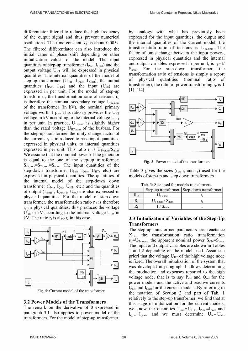
3.2 Power Models of the Transformers The remark on the derivative of θ expressed in

paragraph 3.1 also applies to power model of the

transformers. For the model of step-up transformer,

by analogy with what has previously been

expressed for the input quantities, the output and

the internal quantities of the current model, the

transformation ratio of tensions is UTe,nom. The

factor of units change between the input powers,

expressed in physical quantities and the internal

and output variables expressed in per unit, is rP=1/

Snom. For the step-down transformer, the

transformation ratio of tensions is simply a report

of physical quantities (nominal ratio of

transformer), the ratio of power transforming rP is 1

[1], [14].

Fig. 5: Power model of the transformer.

Table 3 gives the sizes (rU, rI and rP) used for the

models of step-up and step down transformers.

Tab. 3: Size used for models transformers.

Step-up transformer Step-down transformer

RU UTe,nom ra

RI UTe,nom / Snom ra

RP 1 / Snom 1

3.3 Initialization of Variables of the Step-Up

Transformers The step-up transformer parameters are: reactance

XTe, the transformation ratio transformation

rU=UTe,nom, the apparent nominal power SnTe=Snom.

The input and output variables are shown in Tables

1 and 2 depending on the model used. Assume a

priori that the voltage UHT of the high voltage node

is fixed. The overall initialization of the system that

was developed in paragraph 1 allows determining

the production and expenses reported to the high

voltage node, that is to say Pnet and Qnet for the

power models and the active and reactive currents

IPnet and IQnet for the current models. By referring to

the notation of Section 2 and part of Tab. 1

relatively to the step-up transformer, we find that at

this stage of initialization for the current models,

we know the quantities Uout ≡UHT, IP,out≡IPnet and

IQ,out≡IQnet, and we must determine Uin ≡Ualt,



IP,in ≡ IP,alt, IQ,in=IQ,alt and the angle θ , noted eθ in the

case of step-up transformer [5].

From (10), Fig. 4 and Tables 1 and 3, we get

U

HTHT

r

UU =' , netPInetP IrI ,,' = and netQInetQ IrI ,,' = . From

(8) and (9) we can then determine Uin≡Ualt and the

internal angle eθ of the transformer by:

( ) ( )2,

2

, ''' netPTenetQTeHTalt IXIXUU ++=

=θ

alt

netPTe

U

IX ,'arcsin

The currents IP,in≡IPalt and IQ,in≡IQalt are obtained by

relations (7). Similarly, referring to the portion of

Tab. 2 relatively to the step-up transformer, it

appears that, for power models, we know the

quantities Uout≡UHT, Pout≡Pnet and Qout≡Qnet, and we

must determine Uin≡Ualt, Pin≡Palt, Qin≡Palt and the

angle 0e. Relation (16) determines Palt (Pin≡Pout),

and we get U’HT ≡Uout from (15) and the angle eθ is

obtained from equation (23). Knowing Palt, U’HT and

θe we determine Ualt≡Uin from equation (13). Hence

the expression (14) calculates Qin, that is to say the

reactive production Qalt of the alternator [3], [11].

3.4 Initialization of Variables of Charges

and Step-Down Transformers Regarding the initialization of variable charges and

step-down transformers, different approaches are

possible depending on the perspective adopted and

the quantities that are initially binded. For each

approach considered here, the nominal voltage

charge Uch,nom is assumed known. Tables 4 (current

models) and 5 (power models) below summarize

the four approaches we have considered (for current

and power models) based on data and quantities to

be determined. The fact that there are several

approaches shows that in the model structures,

there are several degrees of freedom. For the

approaches 1 and 4, the values of currents or power

charges are given, while for approaches 2 and 3

they are the nominal quantities (at nominal voltage)

that are given. The approaches 1 and 4 are therefore

used in calculating charge flow. For approach 1, the

quantities are given to busbar HT, while for the

approach 4, they are the terminals of the charge. In

this study, for calculations, we have used the

approach 4, which is closest to the methods used in

practice for charge flow calculations [4].

Tab. 4: Approximations of the models.

Given Quantities to

determine

Approximation

1

UHT , IPchHT IQchHT U ch, IPch, IQch, IPch,nom IQch,nom θa

Approximation

2

U c h , IPch,nom , IQch, nom U HT, IPch, IQch ,IPchHT

IQchHT , θa

Approximation

3

UHT, IPch,nom , IQch, nom U ch IPch, IQch IPchHT

IQchHT θa

Approximation

4

UHT , IPch, IQch U ch, IPch,nom, IQch,nom IPchHT , IQchHT, θa

The step-down transformer parameters are: the

reactance XTa, the transformation ratio ra, the

apparant power SnTa=Snom.

Tab. 5: Approximations of the models.

Given Quantities to determine

Approximation

1 UH T , PchHT, IQchHT Uch Pch, Qch Pch,nom

Qch,nom , θa

Approximation

2 Pch , Pch,nom ,

Qch,nom

UH T , Pch , Qch

PchHT , QchHT

θa

Approximation

3 UH T , Pch,nom,

Qch,nom

Uch , Pch , Qch

PchHT QchHT, θa

Approximation

4

UH T , Pch , Qch Uch Pch,nom, Qch,nom,

PchHT ,QchHT , θa

3.4.1 Current models 1

st approache: Starting from the high voltage

node (HV), we give a priori the voltage UH T and

the active current IP c h H T and reactive current

IQ c h H T . Using the notation of Table 1, we therefore

know UHT, IPchHT and IQ c h H T . The problem is to

determine Uch, IQch and the angle θ, noted θa in the

case of step-down transformer. The sum of the

equations squares from the (7) allows to write:

2222

'' QchPchQchHTPchHT IIII +=+ (26)

Similarly, the sum of the equations squares from

the relations (8) and (9) gives:

( ) ( )222''' PchTaQchTachHT IXIXUU ++= (27)

From these last two relations, (26) and (27), we get

I’Pch and I

’Qch and we calculate the currents IPch and

IQCh dividing these values by ra. The angle θa is

given by (8) and the voltage Uch is derived from (9)

and (10). We have also obtained the active and

reactive current, IPch and IQch, of the charge and its

operating voltage Uch. With the characteristic

equations of the charges written here, given that the

initial frequency is the nominal frequency f0:

α

=

nomch

chnomPchPch

U

UII

,

, (28)



β

=

nomch

chnomQchQch

U

UII

,

, (29)

we calculate the values IPch,nom and IQch,nom of the

charge at the nominal voltage

2nd

approache: starting from the charge, we are

given a priori the quantities IPch,nom, IQch,nom and Uch

of the charge. In this case, the active and reactive

currents IPch and IQch of the load are calculated using

relations (28) and (29). We know then Uout≡Uch,

IP,out≡IPch and IQ,out≡IQch, and we determine Uin≡UHT,

θa, IP,in≡IPchH T and IQ,in≡IQchH T in the same manner

as the description of the current models. This gives

UHT, IPchHT and IQchHT.

3rd

approache: we are given a priori the

nominal values IPch,nom, IQch,nom of the load, and we

assume the tension UHT of the node HT as known

(achieved in practice by setting production groups).

This approach requires the simultaneous

initialization of the step-down transformer and the

charge. It remains to be determined Uch, θa, IPchHT,

IQchHT, IpCh and IQch. Using the notation of Tab. 1,

relations (10), (28) and (29) are written [4]:

U i n ≡U H T

α

=

nomch

chnomPchPch

U

UII

,

, (30)

β

=

nomch

chnomQchQch

U

UII

,

, (31)

β

=

nomch

chnomQchQch

U

UII

,

, (32)

U c h =raU’c h

Substituting the previous expressions of I P,out≡IPch

and IQ,out≡IQch in equation (27) yields:

0'''

'2''

2

2

,

,2

2

,

,2

,

,2

=−

+

⋅⋅+

⋅⋅⋅⋅+

βα

β

HT

nomch

chnomPch

nomch

chnomPch

aTa

nomch

chnomQchaTachch

UU

raUI

U

raUI

rXU

raUIrXUU

(32)

We obtain an equation with one unknown

(U’ch≡U’out) whose exponents for various terms in

the equation are: 2, 1+β, 2α , 2β and 0. The

equation (32) has no general analytical solution.

Carrying out an iterative calculation, it is possible

to solve it. However, this equation is readily soluble

in many practical cases:

For α=0 (charge at active power constant). If

β=0, equation (32) becomes a quadratic equation in

U`out, which is easily soluble. If β=1, equation (32)

is also a quadratic equation in U`out, so readily

soluble. If β=2, there is a fourth degree equation

whose analytical solution is expressed not so

simple. If β = 3, the equation is of degree six.

For α =1 or α =2 (charge at constant active

current (=1) or constant impedance (α =2)). If β=0,

the equation (32) is a quadratic equation in U`ch for

a charge at constant active current (=1). By cons,

for a charge at constant impedance (=2), the

equation (32) is an equation of fourth degree in U`ch


simple. If β=1, it remains either a quadratic

equation in U`ch (α =1), or a quadratic equation in

U`2ch (α =2) which are both readily soluble. If β=2,

we get an equation of fourth degree in U`ch whose

analytical solution is expressed not so simple. If

β=3, we can be reducing to a cubic equation in

U`2ch. Table 6 summarizes the situations where the

resolution of equation (32) is easy (sign *).

Tab. 6: The situations where the resolution of equation

(32) is easy.

β

α

0 1 2

0 * *

1 * * *

2

Having determined U'ch≡U'out, we obtain the output

voltage Uout≡Uch by (15). The characteristic

equations of charges (28) and (29) allow to

calculate IP,out≡IPch and lQ,out≡IQch. Hence, we

determine successively the internal angle θa of the

step-down transformer by (8), and the current IP,in ≡

IPchHT and IQ,in≡IQchHT by (7).

4th approache: we start from the charge, for

which we fix the active and reactive currents IPc h

and IQ c h and the nominal voltage Uch,nom and we

assume as known the tension UHT of the node HT.

As the third approach, it also requires the

initialization of both the step-down transformer and

charge. We know here Uin≡UHT and it remains to

determine Uch, θa, IPchHT, I QchHT, IPch,nom and IQ c h ,nom.

From relation (27), taking into consideration the

relation (10) and the fact that the currents I 'P c h and

I 'Q c h respectively represent the products of IPc h

and IQ c h and with the transformation ratio ra, we

get:

( )22

2

PchaTaQchaTa

a

chHT IrXIrX

r

UU +

+= (33)



This quadratic equation in U 2ch provides the tension

of the charges Uch≡Uout. The currents I'Pch and I'Qch

are obtained from IPc h , IQ c h and ra. The angle θa is

given by (8), the currents IPchHT≡IP,in and IQchHT≡IQ,in

are given by relations (7). We finally calculate the

currents IPch,nom and IQch,nom by relations (28) and

(29).

3.4.2 Power Models 1

st approache: starting from the high voltage

node (HT), we are given a priori tension UHT and

the active and reactive powers PchHT and QchHT.

Using the notation of Tab. 2, we therefore know

Uin≡UHT, Pin≡PPchHT and Qin≡QchHT. We have to

determine Uout≡Uch, Pout≡Pch and Qout≡Qch and the

internal angle θa. Relation (12) allows us to

calculate the power Pch≡Pout≡Pin≡PPchHT. By making

the sum of the squares of relations (12) and (14) we

obtain:

2

222

22 '

Ta

chHT

Ta

HTchHTchHT

X

UU

X

UQP

⋅=

−+

This allows us to calculate U'ch=U'out. The relation

(15) provides then Uch=Uout. Relation (12) gives the

internal angle θa and the reactive power Qch=Qout is

determined from the relation (13). This resulted in

the active and reactive powers Pch and Qch of the

charge and also it’s operating voltage Uch. With the

charges characteristics equations (20) and (21) that

are written here, given that the initial frequency is

the nominal frequency f0 :

α

=

nomch

chnomchch

U

UPP

,

, (34)

β

=

nomch

chnomchch

U

UQQ

,

, (35)

We calculate the values Pch,nom and Qch,nom of the

charge at the nominal voltage.

2nd

approache: we start from the charge and we

are given a priori the quantities Pch,nom, Qch,nom

and Uch of the charge. In this case, the active and

reactive powers of the charge Pch and Qch are

calculated using relations (34) and (35). We have to

determine Uout≡Uch, Pout≡Pch and Qout≡Qch we get

Uin≡UHT, Pin≡PPchHT in the same is calculated the

same way as the description on the power models

(section 3.2).

3rd

approache: we are given a priori the nominal

values Pch,nom and Qch,nom of the charge and we

assume the tension UHT of the node HT as known

(achieved in practice by setting production groups).

This approach requires the simultaneous

initialization of the step-down transformer and the

charge. It remains to be determined Uch, θa, PchHT,

QchHT, Pch and Qch. Using the notation of Tab. 1,

relations (15), (34) and (35) are written:

α

=

nomch

chnomchch

U

UPP

,

, (36)

β

=

nomch

chnomchch

U

UQQ

,

, (37)

chach UrU '=

Given Uin≡UHT, and replacing the previous

expressions of Pout≡Pch and Qout≡Qch in equation

(19) we have:

0''

'2

''

2

,

0,2

2

,

,2

2

,

,

2

2

4

=

⋅⋅+

⋅⋅

+

−

⋅⋅⋅+

βα

β

nomch

chach

nomch

chanomch

Ta

HT

nomch

chanomch

Ta

ch

Ta

ch

U

UrQ

U

UrP

X

U

U

UrQ

X

U

X

U

(38)

We obtain an equation with one unknown (U’out≡

U’

c h ) whose exponents for various terms in the

equation are: 4, 2+β, 2, 2 and 2β. Equation (38) has

no general analytical solution. In carrying out an

iterative calculation, it is possible to solve it.

However, this equation is readily soluble in many

practical cases [5]:

For α =0 (charge at constant active power). If

β =0, equation (38) becomes a quadratic equation

in U’ch2 which is easily soluble. If β =1, we have a

fourth degree equation whose analytical solution is

expressed not so simple. If β =2, equation (38) is

also a quadratic equation in U’ch2

therefore easily

soluble. If β =3, we are dealing with an equation

of six degree.

For α =1 or α =2 (charge at constant active

current (α =1) or constant impedance (α =2)). If

β =0, the equation (38) is a quadratic equation in

U’ch2. If β =1, we divide equation (38) by U’ch

2 and

we get a quadratic equation in U’ch. If β =2, we

divide equation (38) by U’ch2 and obtain an

equation of first degree in U’ch2 that solves easily. If

β =3, it can be reduced to a fourth degree equation


simple. Table 7 below summarizes the situations

where the resolution of equation (38) is easy (sign

*).



Tab.7: The situations where the resolution of equation

(38) is easy.

β

α

0 1 2

0 * * *

1 * *

2 * * *

Having determined U`out we obtain the output voltage

Uout≡Uch by (15). The characteristic equations of charges

(36) and (37) allow the calculation of Pout≡Pch and

Qout≡Qch. Hence, we successively determine the angle θa

by (23), Qch≡QchH T by (14) Pin and Pin≡Pc h H T≡Pout by

(12).

4th approache: we start from the charge, for

which we fixe the active and reactive powers Pch

and Qch (assuming the voltage Uch,nom known), and

we assume the tension UHT of the node HT as

known. Knowing Pout≡Pch and Qout≡Qch and also

Uin≡UHT the relation (20) determines U'out≡U'ch and

the relation (15) gives Uout≡Uch. The angle θa of the

step-down transformer is given by (23), QchH T≡Qin is

calculated from (25) and PchH T≡Pin≡Pout is given by (12).

Finally, the relations (36) and (37) allow the calculation of

Pch,nom and Qch,nom.

4 Ideal Transformers The ideal transformer shown schematically in

Figures 6 and 7 corresponds to that of paragraph 2

where the reactance X is zero. This model retains

the active and reactive powers, and also the

frequency and phase. The voltage output (Uout) is

equal to the input voltage (Uin) multiplied by the

transformation ratio (r). The ratio of output current

and input current is the inverse transformation ratio

(1/r).

4.1 Current Model of the Ideal Transformer The input quantities of the current model of the

ideal step-up transformer are the active and reactive

currents IPnet (kA) and IQnet (kA), the voltage Ualt

(p.u.) and the frequency deviation ∆falt (Hz). To

express the output quantities, active and reactive

current IPnet (kA) and IQnet (kA), in quantities per

unit, we must introduce the conversion factor

rI=UTe,nom /Snom between currents. The relationship

between the voltages is rU=UTe,nom. The current

model of ideal step-down transformer has for the

inputs the active and reactive current réactif IPch

(kA) and IQch (kA), voltage UHT (kV) and frequency

deviation ∆fHT (Hz). The output quantities are

IPchHT=ra× IPch, IQch=ra× IQch, Uch=ra×UHT and

∆fch=∆fHT. For step-down transformer, we have

rI=ra and rU=ra. Fig. 6 and Tab. 3 summarize these

results [6].

Fig. 6: Current model of the ideal transformer.

4.2 Power Model of the Ideal Transformer The power model of the step-up transformer has for

inputs the active and reactive powers Pnet (MW) and

Qnet (Mvar), the voltage Ualt (p.u.) and the

frequency deviation ∆falt (Hz). For obtaining the

active and reactive powers Palt and Qalt in quantities

per unit to the exit, we must introduce the

conversion factor rP=1/Snom. The relationship

between the voltages is rU=UTe,non. As the power

model of ideal step-down transformer has entries

for the active and reactive power Pch (MW) et Qch

(Mvar), UHT voltage (kV) and frequency deviation

∆fHT (Hz), the output quantities are PchHT=Pch,

QchHT=Qch, Uch=ra×UHT and ∆fch=∆fHT. For the step-

down transformer, we have rU=ra a n d r P = l . Fig. 7

and Tab. 3 summarize these results.

Fig. 7: Power model of the ideal transformer.

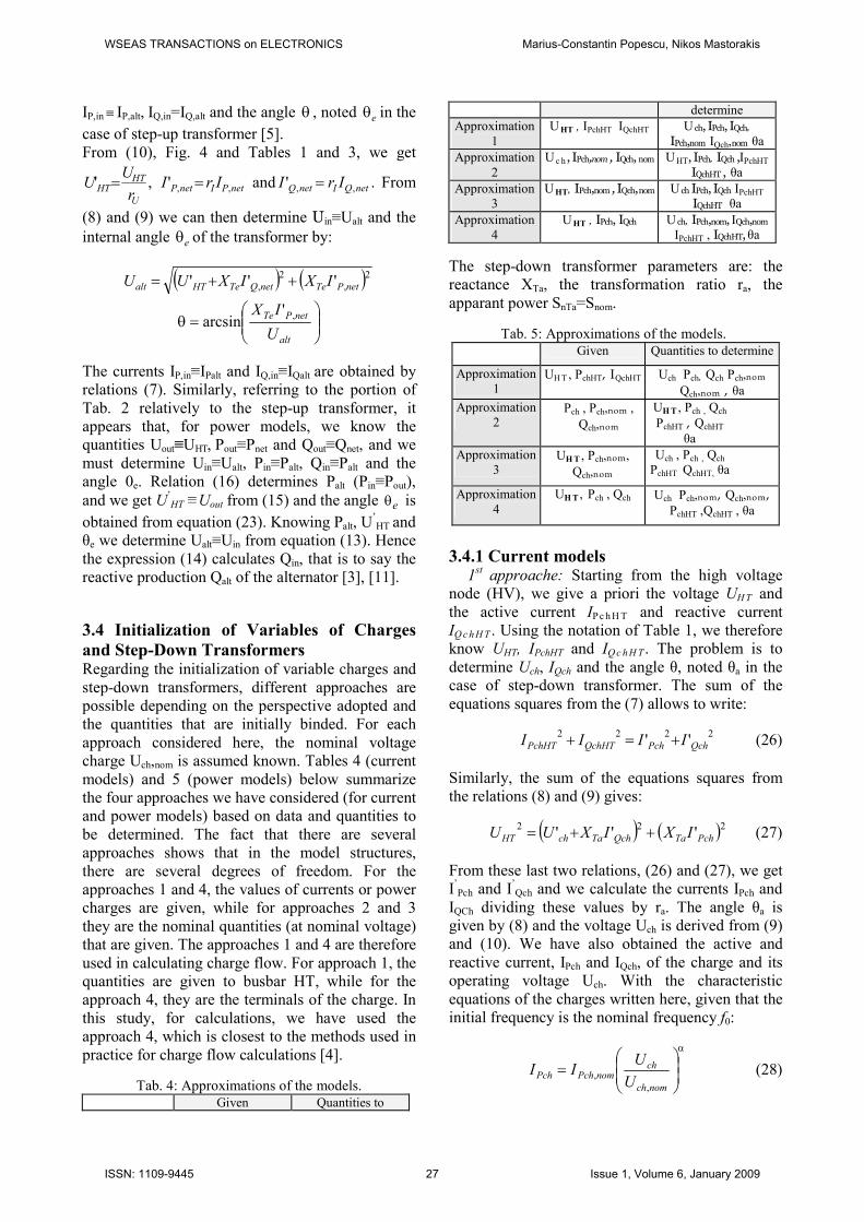
5 Simulations This demonstration illustrates the use of the linear

transformer to simulate a three-winding distribution

transformer rated 75 kVA - 14400/120/120 V (Fig.

8). The transformer primary is connected to a high

voltage source (14,400 V rms). Two identical

inductive loads (20 kW -10 kvar) are connected to

the two secondaries. A third capacitive load (30 kW

-20 kvar) is fed at 240 V. Initially, the circuit

breaker in series with Load 2 is closed, so that the

system is balanced [17]. Open the powergui block



to obtain the initial voltage and current phasors in

steady state [8], [10].

Fig. 8: Transformer model in Simulink.

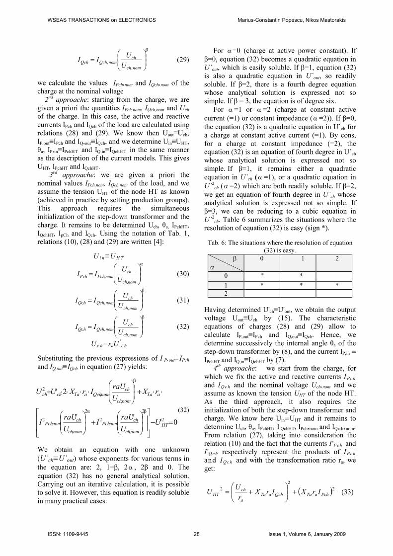
Fig. 9: Linear transformer by Simulink.

As loads are balanced the neutral current is

practically zero. Furthermore, as the inductive

reactive power of Load 1 and Load 2 (2× 10 kvar)

is compensated by the capacitive reactive power of

Load 3 (20 kvar), the primary current is almost in

phase with voltage. The small phase shift (-2.8 deg)

is due to the reactive power associated with

transformer reactive losses. Open the two scopes

and start the simulation. The following observations

can be made: when the circuit breaker opens, a

current starts to flow in the neutral as a result of the

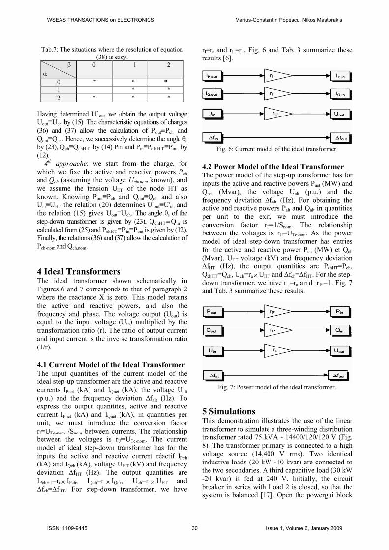
load unbalance. The active power computed from

the primary voltage and current is measured by a

Simulink block which can be found in the

Extras/Measurement library. When the breaker

opens, the active power decreases from 70 kW to

50 kW.

Fig. 10: Parameters transformer.

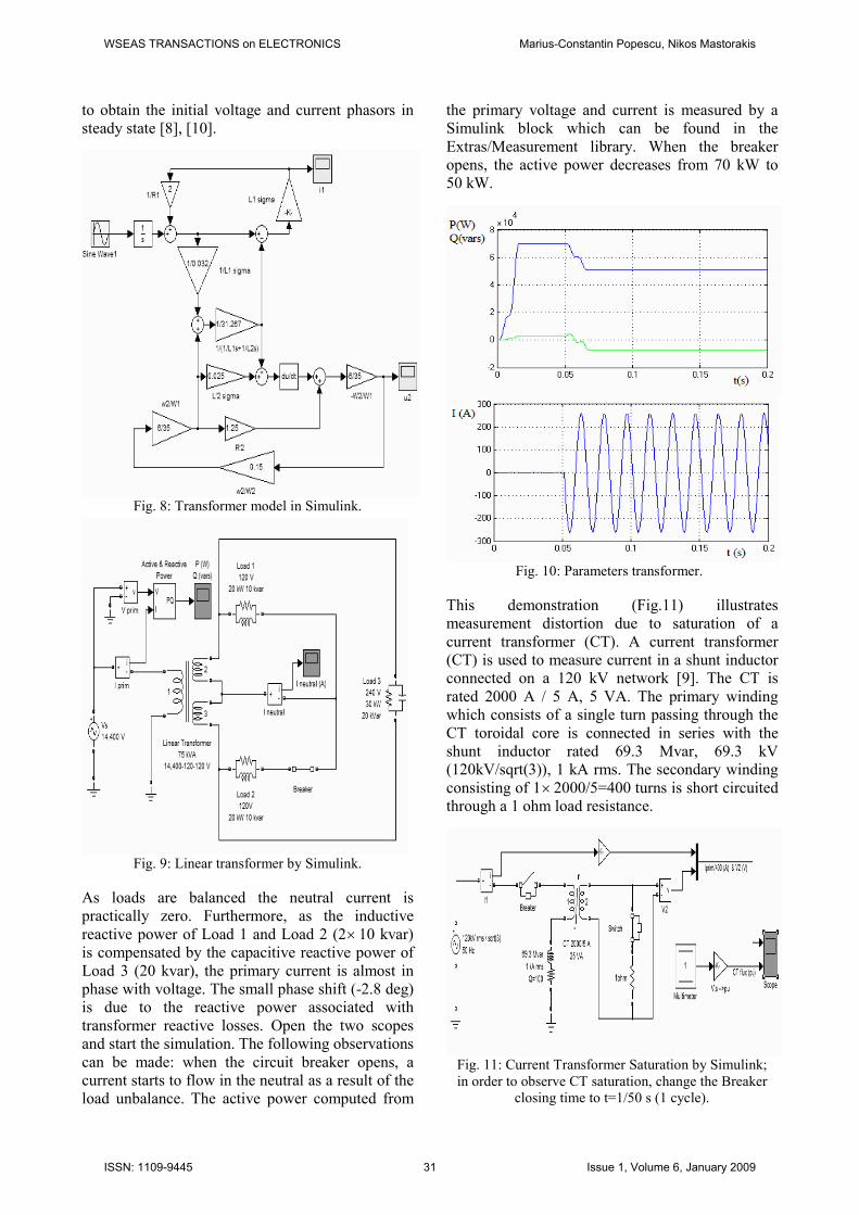
This demonstration (Fig.11) illustrates

measurement distortion due to saturation of a

current transformer (CT). A current transformer

(CT) is used to measure current in a shunt inductor

connected on a 120 kV network [9]. The CT is

rated 2000 A / 5 A, 5 VA. The primary winding

which consists of a single turn passing through the

CT toroidal core is connected in series with the

shunt inductor rated 69.3 Mvar, 69.3 kV

(120kV/sqrt(3)), 1 kA rms. The secondary winding

consisting of 1× 2000/5=400 turns is short circuited

through a 1 ohm load resistance.

Fig. 11: Current Transformer Saturation by Simulink;

in order to observe CT saturation, change the Breaker

closing time to t=1/50 s (1 cycle).



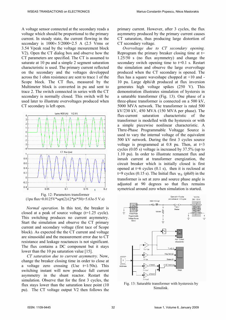
A voltage sensor connected at the secondary reads a

voltage which should be proportional to the primary

current. In steady state, the current flowing in the

secondary is 1000× 5/2000=2.5 A (2.5 Vrms or

3.54 Vpeak read by the voltage mesurement block

V2). Open the CT dialog box and observe how the

CT parameters are specified. The CT is assumed to

saturate at 10 pu and a simple 2 segment saturation

characteristic is used. The primary current reflected

on the secondary and the voltages developped

across the 1 ohm resistance are sent to trace 1 of the

Scope block. The CT flux, measured by the

Multimeter block is converted in pu and sent to

trace 2. The switch connected in series with the CT

secondary is normally closed. This switch will be

used later to illustrate overvoltages produced when

CT secondary is left open.

Fig. 12: Parameters transformer

(1pu flux=0.0125V*sqrt(2)/(2*pi*50)=5.63e-5 V.s)

Normal operation. In this test, the breaker is

closed at a peak of source voltage (t=1.25 cycle).

This switching produces no current asymmetry.

Start the simulation and observe the CT primary

current and secondary voltage (first tace of Scope

block). As expected the the CT current and voltage

are sinusoidal and the measurement error due to CT

resistance and leakage reactances is not significant.

The flux contains a DC component but it stays

lower than the 10 pu saturation value [15].

CT saturation due to current asymmetry. Now,

change the breaker closing time in order to close at

a voltage zero crossing (Use t=1/50s). This

switching instant will now produce full current

asymmetry in the shunt reactor. Restart the

simulation. Observe that for the first 3 cycles, the

flux stays lower than the saturation knee point (10

pu). The CT voltage output V2 then follows the

primary current. However, after 3 cycles, the flux

asymmetry produced by the primary current causes

CT saturation, thus producing large distortion of

CT secondary voltage.

Overvoltage due to CT secondary opening.

Reprogram the primary breaker closing time at t=

1.25/50 s (no flux asymmetry) and change the

secondary switch opening time to t=0.1 s. Restart

the simulation and observe the large overvoltage

produced when the CT secondary is opened. The

flux has a square waveshape chopped at +10 and -

10 pu. Large dphi/dt produced at flux inversion

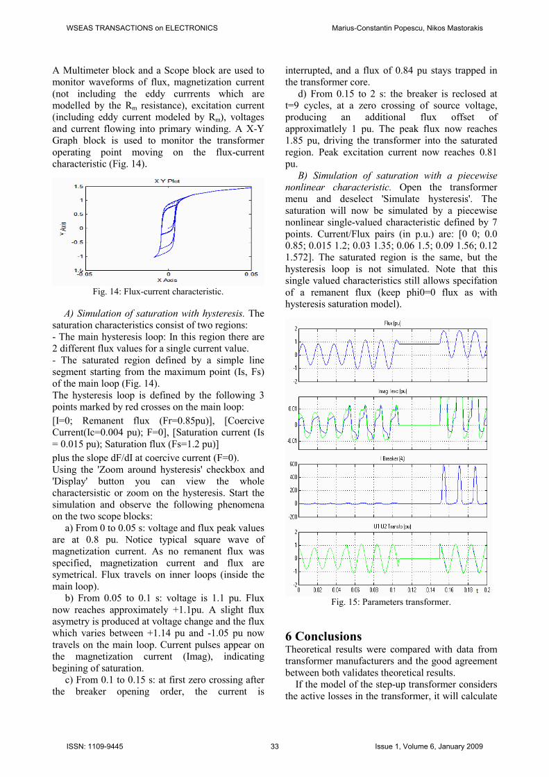
generates high voltage spikes (250 V). This

demonstration illustrates simulation of hystersis in

a saturable transformer (Fig. 13). One phase of a

three-phase transformer is connected on a 500 kV,

5000 MVA network. The transformer is rated 500

kV/230 kV, 450 MVA (150 MVA per phase). The

flux-current saturation characteristic of the

transformer is modelled with the hysteresis or with

a simple piecewise nonlinear characteristic. A

Thrre-Phase Programmable Voltagge Source is

used to vary the internal voltage of the equivalent

500 kV network. During the first 3 cycles source

voltage is programmed at 0.8 pu. Then, at t=3

cycles (0.05 s) voltage is increased by 37.5% (up to

1.10 pu). In order to illustrate remanent flux and

inrush current at transformer energization, the

circuit breaker which is initially closed is first

opened at t=6 cycles (0.1 s), then it is reclosed at

t=9 cycles (0.15 s). The Initial flux 0ψ (phi0) in the

transformer is set at zero and source phase angle is

adjusted at 90 degrees so that flux remains

symetrical around zero when simulation is started.

Fig. 13: Saturable transformer with hysteresis by

Simulink.



A Multimeter block and a Scope block are used to

monitor waveforms of flux, magnetization current

(not including the eddy currrents which are

modelled by the Rm resistance), excitation current

(including eddy current modeled by Rm), voltages

and current flowing into primary winding. A X-Y

Graph block is used to monitor the transformer

operating point moving on the flux-current

characteristic (Fig. 14).

Fig. 14: Flux-current characteristic.

A) Simulation of saturation with hysteresis. The

saturation characteristics consist of two regions:

- The main hysteresis loop: In this region there are

2 different flux values for a single current value.

- The saturated region defined by a simple line

segment starting from the maximum point (Is, Fs)

of the main loop (Fig. 14).

The hysteresis loop is defined by the following 3

points marked by red crosses on the main loop:

[I=0; Remanent flux (Fr=0.85pu)], [Coercive

Current(Ic=0.004 pu); F=0], [Saturation current (Is

= 0.015 pu); Saturation flux (Fs=1.2 pu)]

plus the slope dF/dI at coercive current (F=0).

Using the 'Zoom around hysteresis' checkbox and

'Display' button you can view the whole

charactersistic or zoom on the hysteresis. Start the

simulation and observe the following phenomena

on the two scope blocks:

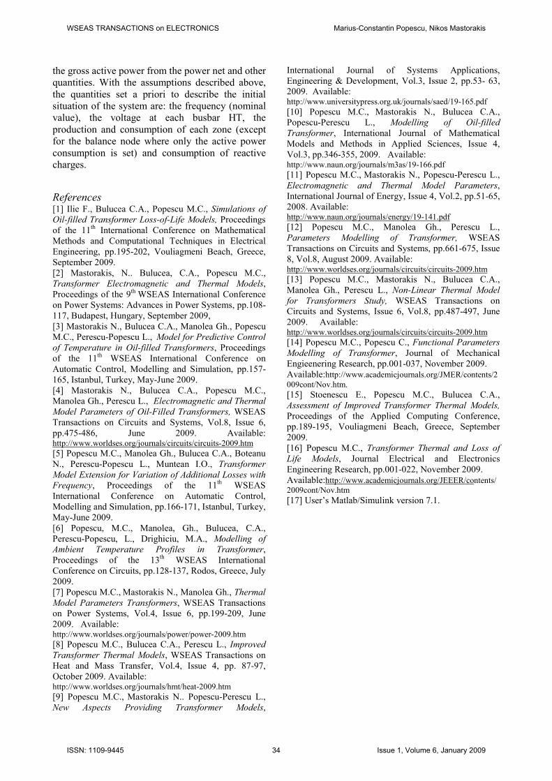
a) From 0 to 0.05 s: voltage and flux peak values

are at 0.8 pu. Notice typical square wave of

magnetization current. As no remanent flux was

specified, magnetization current and flux are

symetrical. Flux travels on inner loops (inside the

main loop).

b) From 0.05 to 0.1 s: voltage is 1.1 pu. Flux

now reaches approximately +1.1pu. A slight flux

asymetry is produced at voltage change and the flux

which varies between +1.14 pu and -1.05 pu now

travels on the main loop. Current pulses appear on

the magnetization current (Imag), indicating

begining of saturation.

c) From 0.1 to 0.15 s: at first zero crossing after

the breaker opening order, the current is

interrupted, and a flux of 0.84 pu stays trapped in

the transformer core.

d) From 0.15 to 2 s: the breaker is reclosed at

t=9 cycles, at a zero crossing of source voltage,

producing an additional flux offset of

approximatlely 1 pu. The peak flux now reaches

1.85 pu, driving the transformer into the saturated

region. Peak excitation current now reaches 0.81

pu.

B) Simulation of saturation with a piecewise

nonlinear characteristic. Open the transformer

menu and deselect 'Simulate hysteresis'. The

saturation will now be simulated by a piecewise

nonlinear single-valued characteristic defined by 7

points. Current/Flux pairs (in p.u.) are: [0 0; 0.0

0.85; 0.015 1.2; 0.03 1.35; 0.06 1.5; 0.09 1.56; 0.12

1.572]. The saturated region is the same, but the

hysteresis loop is not simulated. Note that this

single valued characteristics still allows specifation

of a remanent flux (keep phi0=0 flux as with

hysteresis saturation model).

Fig. 15: Parameters transformer.

6 Conclusions Theoretical results were compared with data from

transformer manufacturers and the good agreement

between both validates theoretical results.

If the model of the step-up transformer considers

the active losses in the transformer, it will calculate



the gross active power from the power net and other

quantities. With the assumptions described above,

the quantities set a priori to describe the initial

situation of the system are: the frequency (nominal

value), the voltage at each busbar HT, the

production and consumption of each zone (except

for the balance node where only the active power

consumption is set) and consumption of reactive

charges.

References [1] Ilie F., Bulucea C.A., Popescu M.C., Simulations of

Oil-filled Transformer Loss-of-Life Models, Proceedings

of the 11th

International Conference on Mathematical

Methods and Computational Techniques in Electrical

Engineering, pp.195-202, Vouliagmeni Beach, Greece,

September 2009.

[2] Mastorakis, N.. Bulucea, C.A., Popescu M.C.,

Transformer Electromagnetic and Thermal Models,

Proceedings of the 9th

WSEAS International Conference

on Power Systems: Advances in Power Systems, pp.108-

117, Budapest, Hungary, September 2009,

[3] Mastorakis N., Bulucea C.A., Manolea Gh., Popescu

M.C., Perescu-Popescu L., Model for Predictive Control

of Temperature in Oil-filled Transformers, Proceedings

of the 11th

WSEAS International Conference on

Automatic Control, Modelling and Simulation, pp.157-

165, Istanbul, Turkey, May-June 2009.

[4] Mastorakis N., Bulucea C.A., Popescu M.C.,

Manolea Gh., Perescu L., Electromagnetic and Thermal

Model Parameters of Oil-Filled Transformers, WSEAS

Transactions on Circuits and Systems, Vol.8, Issue 6,

pp.475-486, June 2009. Available: http://www.worldses.org/journals/circuits/circuits-2009.htm [5] Popescu M.C., Manolea Gh., Bulucea C.A., Boteanu

N., Perescu-Popescu L., Muntean I.O., Transformer

Model Extension for Variation of Additional Losses with

Frequency, Proceedings of the 11th

WSEAS

International Conference on Automatic Control,

Modelling and Simulation, pp.166-171, Istanbul, Turkey,

May-June 2009.

[6] Popescu, M.C., Manolea, Gh., Bulucea, C.A.,

Perescu-Popescu, L., Drighiciu, M.A., Modelling of

Ambient Temperature Profiles in Transformer,

Proceedings of the 13th

WSEAS International

Conference on Circuits, pp.128-137, Rodos, Greece, July

2009.

[7] Popescu M.C., Mastorakis N., Manolea Gh., Thermal

Model Parameters Transformers, WSEAS Transactions

on Power Systems, Vol.4, Issue 6, pp.199-209, June

2009. Available: http://www.worldses.org/journals/power/power-2009.htm

[8] Popescu M.C., Bulucea C.A., Perescu L., Improved

Transformer Thermal Models, WSEAS Transactions on

Heat and Mass Transfer, Vol.4, Issue 4, pp. 87-97,

October 2009. Available: http://www.worldses.org/journals/hmt/heat-2009.htm

[9] Popescu M.C., Mastorakis N.. Popescu-Perescu L.,

New Aspects Providing Transformer Models,

International Journal of Systems Applications,

Engineering & Development, Vol.3, Issue 2, pp.53- 63,

2009. Available: http://www.universitypress.org.uk/journals/saed/19-165.pdf

[10] Popescu M.C.,

Mastorakis N., Bulucea C.A.,

Popescu-Perescu L., Modelling of Oil-filled

Transformer, International Journal of Mathematical

Models and Methods in Applied Sciences, Issue 4,

Vol.3, pp.346-355, 2009. Available: http://www.naun.org/journals/m3as/19-166.pdf

[11] Popescu M.C., Mastorakis N., Popescu-Perescu L.,

Electromagnetic and Thermal Model Parameters,

International Journal of Energy, Issue 4, Vol.2, pp.51-65,

2008. Available: http://www.naun.org/journals/energy/19-141.pdf

[12] Popescu M.C., Manolea Gh., Perescu L.,

Parameters Modelling of Transformer, WSEAS

Transactions on Circuits and Systems, pp.661-675, Issue

8, Vol.8, August 2009. Available: http://www.worldses.org/journals/circuits/circuits-2009.htm

[13] Popescu M.C., Mastorakis N., Bulucea C.A.,

Manolea Gh., Perescu L., Non-Linear Thermal Model

for Transformers Study, WSEAS Transactions on

Circuits and Systems, Issue 6, Vol.8, pp.487-497, June

2009. Available: http://www.worldses.org/journals/circuits/circuits-2009.htm [14] Popescu M.C., Popescu C., Functional Parameters

Modelling of Transformer, Journal of Mechanical

Engieenering Research, pp.001-037, November 2009.

Available:http://www.academicjournals.org/JMER/contents/2

009cont/Nov.htm. [15] Stoenescu E., Popescu M.C., Bulucea C.A.,

Assessment of Improved Transformer Thermal Models,

Proceedings of the Applied Computing Conference,

pp.189-195, Vouliagmeni Beach, Greece, September

2009.

[16] Popescu M.C., Transformer Thermal and Loss of

Life Models, Journal Electrical and Electronics

Engineering Research, pp.001-022, November 2009.

Available:http://www.academicjournals.org/JEEER/contents/

2009cont/Nov.htm [17] User’s Matlab/Simulink version 7.1.



modelling and simulation of stepup and stepdown … and simulation of stepup and stepdown...

Documents