lab 7: raster data analysis - density surfaces lab series gst 102: spatial analysis lab 7: raster...

QGIS LAB SERIESGST 102: Spatial Analysis

Lab 7: Raster Data Analysis - Density Surfaces

Objective – Learn Density Analysis Methods

Document Version: 2014-07-11 (Beta)

ContentsIntroduction.............................................................................................................2Objective: Learn the Basics of Terrain Analysis.....................................................2How Best to Use Video Walk Through with this Lab..............................................2

QGIS LAB SERIES - Lab 8 – Raster Data Analysis - Density Surfaces

Introduction

In this lab the students will learn about performing point density analysis. Density analysis can be used to show areas where there is a high occurrence of data. The lab will cover converting between vector and raster data.

This lab includes the following tasks:

Task 1 Point DensityTask 2 Raster to Vector Conversion Task 3 Vector to Raster Conversion

Objective: Learn the Basics of Terrain Analysis

The objective of this lab is to learn about the density analysis methods and look at the conversion between the raster and vector data models.

How Best to Use Video Walk Through with this Lab

To aid in your completion of this lab, each lab task has an associated video that demonstrates how to complete the task. The intent of these videos is to help you move forward if you become stuck on a step in a task, or you wish to visually see every step required to complete the tasks.

We recommend that you do not watch the videos before you attempt the tasks. The reasoning for this is that while you are learning the software and searching for buttons, menus, etc…, you will better remember where these items are and, perhaps, discover other features along the way. With that being said, please use the videos in the way that will best facilitate your learning and successful completion of this lab.

Task 1 Point Density

Point density analysis can be used to show where there is a concentration of data points. In this task, you will be using a core QGIS plugin called Heatmap, which generates point density surfaces.

Radius (aka neighborhood) – With the Heatmap tool you can define the search radius. The tool will use this distance when searching for neighboring points. A given pixel will receive higher values when more points are found within that search radius, and lower values when fewer points are found. Therefore, you can get very different results by changing the radius value.

1. The data for this lab is located on the lab machine at: C:\GST102\Lab 8\Data.

2. Open QGIS Desktop 2.4.0.

8/30/14 Copyright © 2013 NISGTC of 17


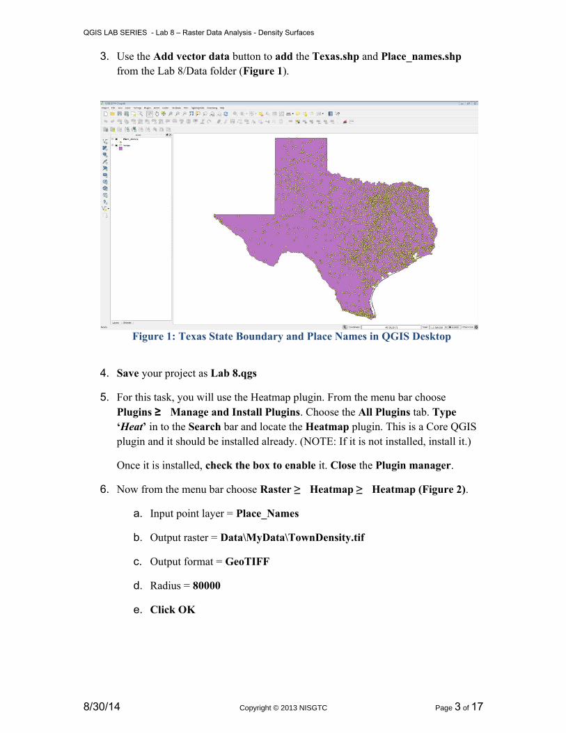
3. Use the Add vector data button to add the Texas.shp and Place_names.shp from the Lab 8/Data folder (Figure 1).

Figure 1: Texas State Boundary and Place Names in QGIS Desktop

4. Save your project as Lab 8.qgs

5. For this task, you will use the Heatmap plugin. From the menu bar choose Plugins Manage and Install Plugins. Choose the All Plugins tab. Type ‘Heat’ in to the Search bar and locate the Heatmap plugin. This is a Core QGIS plugin and it should be installed already. (NOTE: If it is not installed, install it.)

Once it is installed, check the box to enable it. Close the Plugin manager.

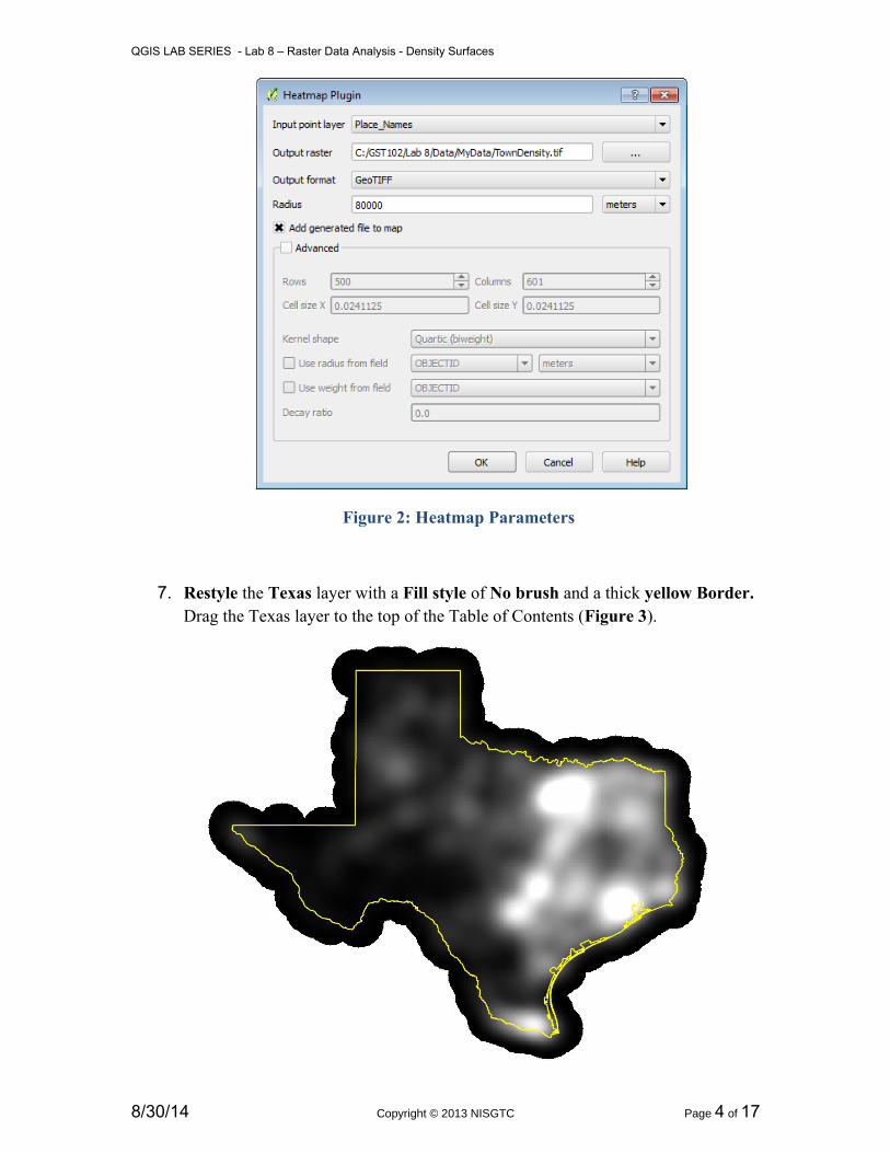
6. Now from the menu bar choose Raster Heatmap Heatmap (Figure 2).

a. Input point layer = Place_Names

b. Output raster = Data\MyData\TownDensity.tif

c. Output format = GeoTIFF

d. Radius = 80000

e. Click OK



Figure 2: Heatmap Parameters

7. Restyle the Texas layer with a Fill style of No brush and a thick yellow Border. Drag the Texas layer to the top of the Table of Contents (Figure 3).



Figure 3: Heatmap from Place Names

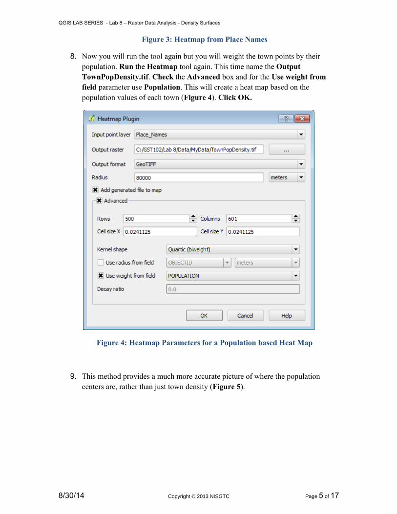
8. Now you will run the tool again but you will weight the town points by their population. Run the Heatmap tool again. This time name the Output TownPopDensity.tif. Check the Advanced box and for the Use weight from field parameter use Population. This will create a heat map based on the population values of each town (Figure 4). Click OK.

Figure 4: Heatmap Parameters for a Population based Heat Map

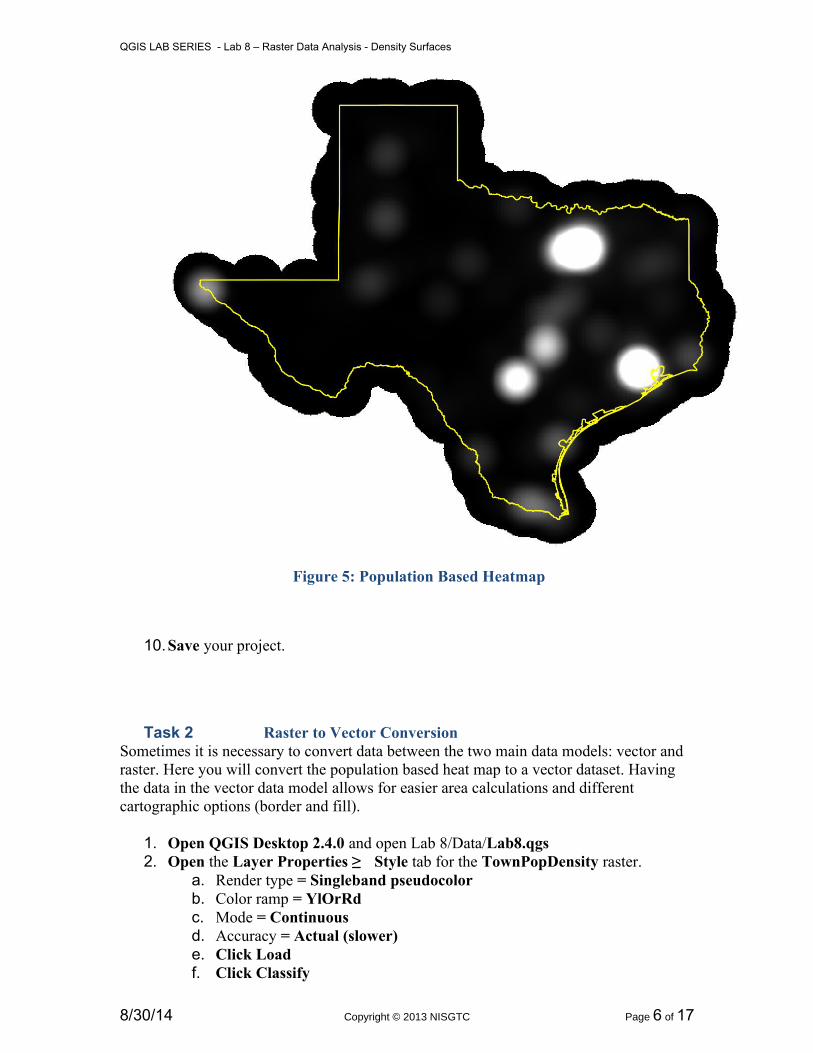
9. This method provides a much more accurate picture of where the population centers are, rather than just town density (Figure 5).



Figure 5: Population Based Heatmap

10.Save your project.

Task 2 Raster to Vector ConversionSometimes it is necessary to convert data between the two main data models: vector and raster. Here you will convert the population based heat map to a vector dataset. Having the data in the vector data model allows for easier area calculations and different cartographic options (border and fill).

1. Open QGIS Desktop 2.4.0 and open Lab 8/Data/Lab8.qgs2. Open the Layer Properties Style tab for the TownPopDensity raster.

a. Render type = Singleband pseudocolorb. Color ramp = YlOrRdc. Mode = Continuousd. Accuracy = Actual (slower)e. Click Loadf. Click Classify



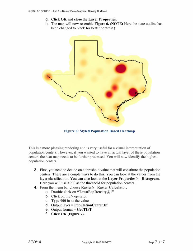
g. Click OK and close the Layer Properties.h. The map will now resemble Figure 6. (NOTE: Here the state outline has

been changed to black for better contrast.)

Figure 6: Styled Population Based Heatmap

This is a more pleasing rendering and is very useful for a visual interpretation of population centers. However, if you wanted to have an actual layer of these population centers the heat map needs to be further processed. You will now identify the highest population centers.

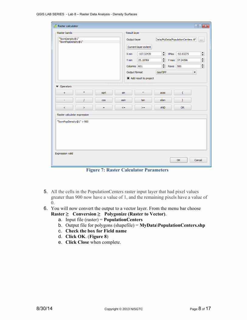
3. First, you need to decide on a threshold value that will constitute the population centers. There are a couple ways to do this. You can look at the values from the layer classification. You can also look at the Layer Properties Histogram. Here you will use >900 as the threshold for population centers.

4. From the menu bar choose Raster Raster Calculator.a. Double click on “TownPopDensity@1”b. Click on the > operatorc. Type 900 in as the valued. Output layer = PopulationCenter.tife. Output format = GeoTIFFf. Click OK (Figure 7).



Figure 7: Raster Calculator Parameters

5. All the cells in the PopulationCenters raster input layer that had pixel values greater than 900 now have a value of 1, and the remaining pixels have a value of 0.

6. You will now convert the output to a vector layer. From the menu bar choose Raster Conversion Polygonize (Raster to Vector).

a. Input file (raster) = PopulationCentersb. Output file for polygons (shapefile) = MyData\PopulationCenters.shpc. Check the box for Field named. Click OK. (Figure 8)e. Click Close when complete.



Figure 8: Raster to Vector Conversion Parameters

7. When the processing is complete, make sure the new polygon layer is above the raster layer in the Table of Contents so that it is visible.

Since the output represents all the pixels in the raster you need to eliminate the non-population center polygons from this layer. To do this you will put the layer into Edit mode, select those polygons with a value of 0 and delete them.

8. Right click on the layer and choose Toggle editing from the context menu.9. Now open the attribute table for the layer. Click the Select features using an

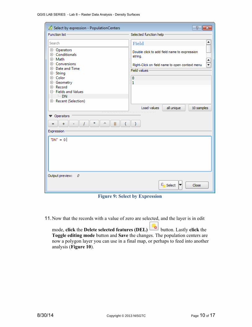
expression button .10.Expand Field and Values. Double click on DN to place it in the Expression

window. Click the = operator. Now click the all unique button and double click on the 0 value to place it in the expression. (Figure 9) Click Select. Click Close.



Figure 9: Select by Expression

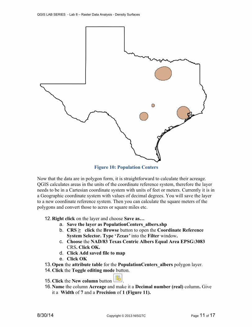
11.Now that the records with a value of zero are selected, and the layer is in edit

mode, click the Delete selected features (DEL) button. Lastly click the Toggle editing mode button and Save the changes. The population centers are now a polygon layer you can use in a final map, or perhaps to feed into another analysis (Figure 10).



Figure 10: Population Centers

Now that the data are in polygon form, it is straightforward to calculate their acreage. QGIS calculates areas in the units of the coordinate reference system, therefore the layer needs to be in a Cartesian coordinate system with units of feet or meters. Currently it is ina Geographic coordinate system with values of decimal degrees. You will save the layer to a new coordinate reference system. Then you can calculate the square meters of the polygons and convert those to acres or square miles etc.

12.Right click on the layer and choose Save as…a. Save the layer as PopulationCenters_albers.shpb. CRS click the Browse button to open the Coordinate Reference

System Selector. Type ‘Texas’ into the Filter window.c. Choose the NAD/83 Texas Centric Albers Equal Area EPSG:3083

CRS. Click OK.d. Click Add saved file to mape. Click OK

13.Open the attribute table for the PopulationCenters_albers polygon layer.14.Click the Toggle editing mode button.

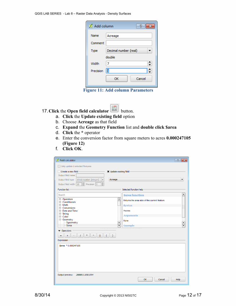
15.Click the New column button .16.Name the column Acreage and make it a Decimal number (real) column. Give

it a Width of 7 and a Precision of 1 (Figure 11).



Figure 11: Add column Parameters

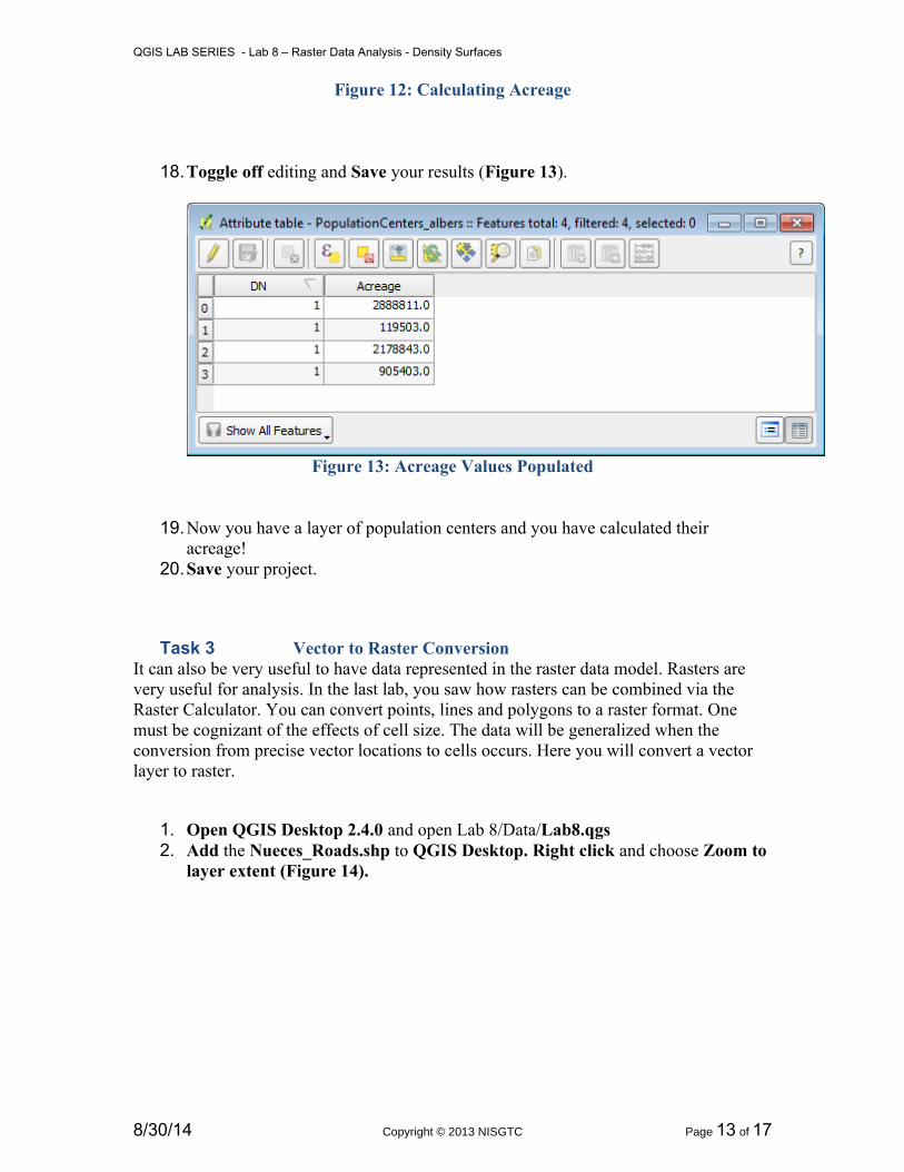
17.Click the Open field calculator button.a. Click the Update existing field optionb. Choose Acreage as that fieldc. Expand the Geometry Function list and double click $aread. Click the * operatore. Enter the conversion factor from square meters to acres 0.000247105

(Figure 12)f. Click OK.



Figure 12: Calculating Acreage

18.Toggle off editing and Save your results (Figure 13).

Figure 13: Acreage Values Populated

19.Now you have a layer of population centers and you have calculated their acreage!

20.Save your project.

Task 3 Vector to Raster ConversionIt can also be very useful to have data represented in the raster data model. Rasters are very useful for analysis. In the last lab, you saw how rasters can be combined via the Raster Calculator. You can convert points, lines and polygons to a raster format. One must be cognizant of the effects of cell size. The data will be generalized when the conversion from precise vector locations to cells occurs. Here you will convert a vector layer to raster.

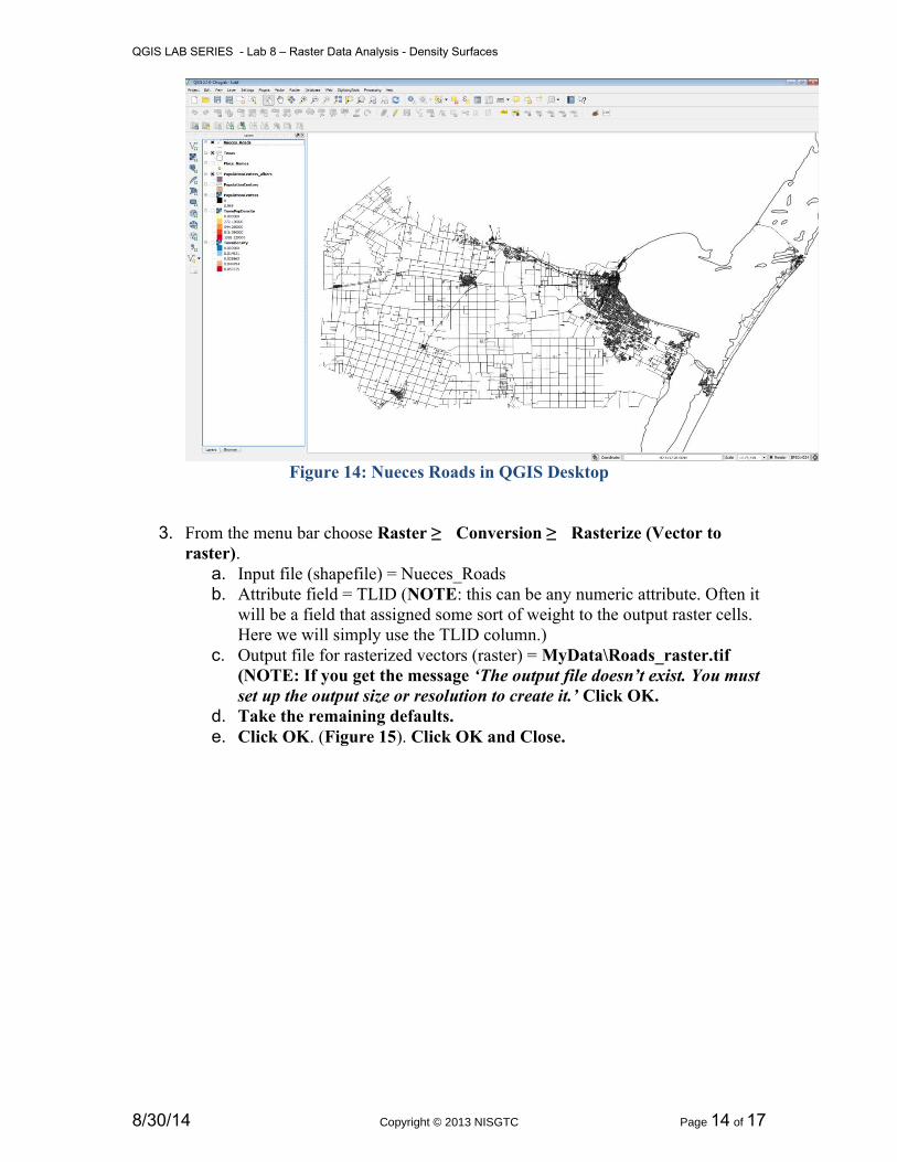
1. Open QGIS Desktop 2.4.0 and open Lab 8/Data/Lab8.qgs2. Add the Nueces_Roads.shp to QGIS Desktop. Right click and choose Zoom to

layer extent (Figure 14).



Figure 14: Nueces Roads in QGIS Desktop

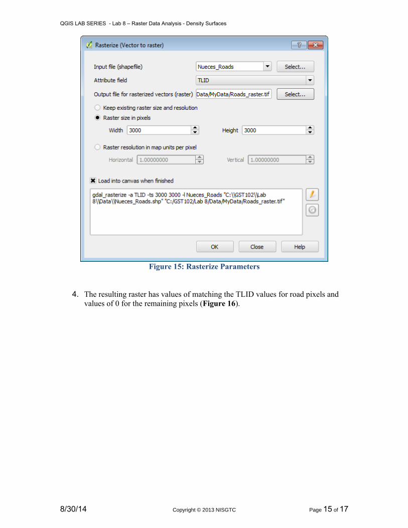
3. From the menu bar choose Raster Conversion Rasterize (Vector to raster).

a. Input file (shapefile) = Nueces_Roadsb. Attribute field = TLID (NOTE: this can be any numeric attribute. Often it

will be a field that assigned some sort of weight to the output raster cells. Here we will simply use the TLID column.)

c. Output file for rasterized vectors (raster) = MyData\Roads_raster.tif (NOTE: If you get the message ‘The output file doesn’t exist. You must set up the output size or resolution to create it.’ Click OK.

d. Take the remaining defaults.e. Click OK. (Figure 15). Click OK and Close.



Figure 15: Rasterize Parameters

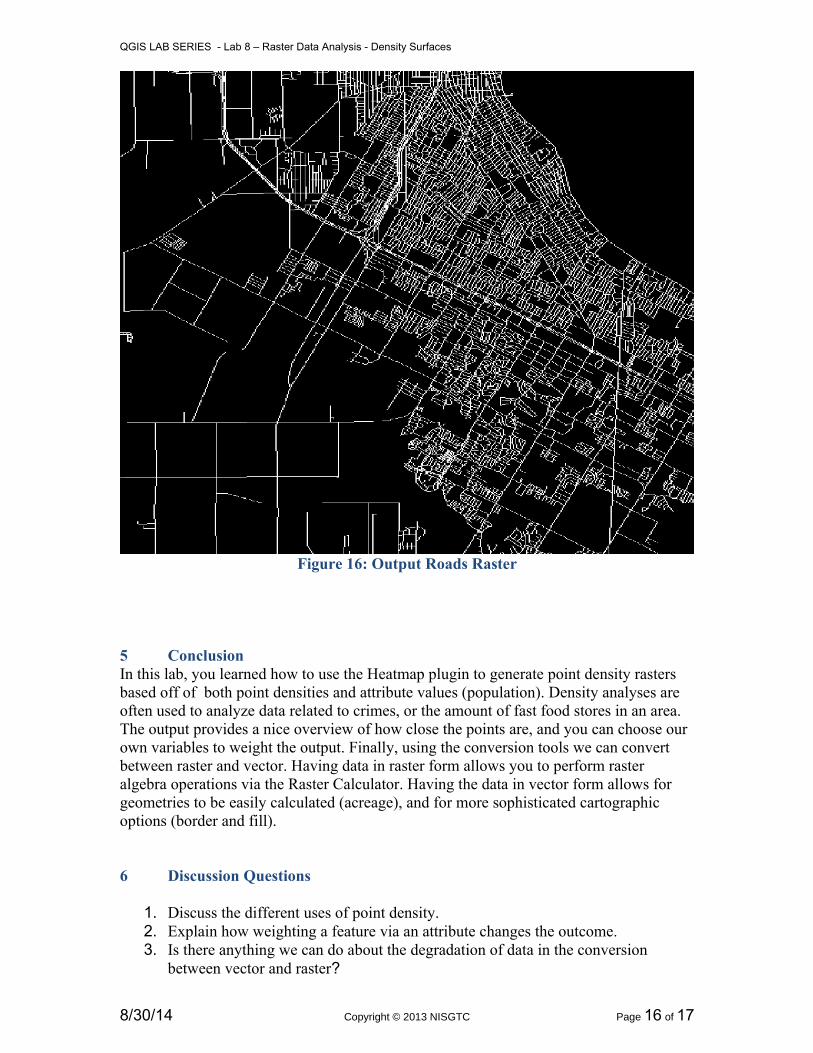
4. The resulting raster has values of matching the TLID values for road pixels and values of 0 for the remaining pixels (Figure 16).



Figure 16: Output Roads Raster

5 ConclusionIn this lab, you learned how to use the Heatmap plugin to generate point density rasters based off of both point densities and attribute values (population). Density analyses are often used to analyze data related to crimes, or the amount of fast food stores in an area. The output provides a nice overview of how close the points are, and you can choose our own variables to weight the output. Finally, using the conversion tools we can convert between raster and vector. Having data in raster form allows you to perform raster algebra operations via the Raster Calculator. Having the data in vector form allows for geometries to be easily calculated (acreage), and for more sophisticated cartographic options (border and fill).

6 Discussion Questions

1. Discuss the different uses of point density.2. Explain how weighting a feature via an attribute changes the outcome.3. Is there anything we can do about the degradation of data in the conversion

between vector and raster?



7 Challenge Assignment

In the Lab8/Data/Challenge folder there is a shapefile containing crime data for Surrey inthe United Kingdom. There is a column for crime type (Crime_type). Use this field togenerate two heatmaps: one for ‘Violent Crimes’ and one for ‘Drugs’. You will have toselect records corresponding to each crime type, and save the selected features to a newshapefile for each. The heatmaps will be generated against the resulting shapefiles.


lab 7: raster data analysis - density surfaces lab series gst 102: spatial analysis lab 7: raster...

Documents