Published in Image Processing On Line on 2015–12–26.Submitted on 2015–04–13, accepted on 2015–08–13.ISSN 2105–1232 c© 2015 IPOL & the authors CC–BY–NC–SAThis article is available online with supplementary materials,software, datasets and online demo athttp://dx.doi.org/10.5201/ipol.2015.136

2015/06/16

v0.5.1

IPOL

article

class

Variational Framework for Non-Local Inpainting

Vadim Fedorov 1, Gabriele Facciolo 2, Pablo Arias 2

1 DTIC, Universitat Pompeu Fabra, Spain (vadim.fedorov@upf.edu)2 CMLA, ENS-Cachan, France (facciolo, pablo.arias@cmla.ens-cachan.fr)

Abstract

Image inpainting aims to obtain a visually plausible image interpolation in a region of the imagein which data is missing due to damage or occlusion. Usually, the only available informationis the portion of the image outside the inpainting domain. Besides its numerous applications,the inpainting problem is of theoretical interest since its analysis involves an understanding ofthe self-similarity present in natural images. In this work, we present a detailed descriptionand implementation of three exemplar-based inpainting methods derived from the variationalframework introduced by Arias et al.

Source Code

The implementation written in C++ for this algorithm is available in the IPOL web page of thisarticle1. Compilation and usage instructions are included in the README.md file of the archive.

Keywords: image inpainting; variational methods; exemplar-based; nonlocal methods

1 Introduction

Image inpainting, also known as image completion, disocclusion or object removal, aims to obtain avisually plausible image interpolation in a region of the image in which data is missing due to damageor occlusion. Usually, to solve this problem, the only available data is the image outside the regionto be inpainted. Inpainting has become a standard tool in digital photography for image retouchingand video post-production. Besides its numerous applications, the problem is of theoretical interestsince its analysis involves an understanding of the self-similarity present in natural images.

1.1 Context: Geometric and Texture Inpainting

Most inpainting methods found in the literature can be classified into two groups: geometry- andtexture-oriented depending on how they characterize the redundancy of the image.

1http://dx.doi.org/10.5201/ipol.2015.136

Vadim Fedorov , Gabriele Facciolo , Pablo Arias , Variational Framework for Non-Local Inpainting, Image Processing On Line, 5 (2015),pp. 362–386. http://dx.doi.org/10.5201/ipol.2015.136

Variational Framework for Non-Local Inpainting

Geometry-oriented methods. In this class of methods images are usually modeled as functionswith some degree of smoothness, expressed for instance in terms of the curvature of the level linesor the total variation of the image. This smoothness assumption is exploited to interpolate theinpainting domain by continuing the geometric structures of the image (its level lines, or its edges),usually by means of a partial differential equation (PDE). Such PDEs can be derived from variationalprinciples [31, 5, 14, 15, 20, 30], or inspired by phenomenological modeling [8, 11, 41]. These methodsshow good performance in propagating smooth level lines or gradients, but fail in the presence oftexture. They are often referred to as structure or cartoon inpainting.

The geometry-oriented methods are said to be local in the sense that among all the data availablefrom the image, they only use the information at the boundary of the inpainting domain.

Texture-oriented methods. Texture-oriented inpainting was born as an application of texturesynthesis [19, 25]. Its recent development was triggered in part by the works of Efros and Leung [19],and Wei and Levoy [42] using non-parametric sampling techniques. In these works texture is modeledas a two dimensional probabilistic graphical model, in which the value of each pixel is conditioned byits neighborhood. These approaches rely directly on a sample of the desired texture to perform thesynthesis. The value of each synthesized pixel x is copied from the center of a patch in the sampleimage, chosen to match the available portion of the patch centered at x.

This strategy has been extensively used for inpainting [9, 10, 16, 18, 19, 35]. As opposed togeometry-oriented inpainting, these so-called exemplar-based approaches are non-local. That is, todetermine the value at x, the whole image may be traversed in the search for a matching patch. Thusthe problem of exemplar-based inpainting can be stated [17] as that of finding a correspondence map

ϕ : O → Oc, which assigns to each point x in the inpainting domain O (a subset of the image domainΩ ⊂ R

2) a corresponding point ϕ(x) ∈ Oc := Ω \ O where the image is known (see Figure 1). Theunknown part of the image is then synthesized using the map ϕ.

Early exemplar-based approaches to image inpainting [19, 42] use greedy procedures for computingthe correspondence map. Their results are very sensitive to the order in which the pixels are processed[16, 35, 23]. To address this issue Demanet et al. [17] proposed to model the inpainting problem asan energy minimization in which the unknown is the correspondence map itself

E(ϕ) =∫

O

∫

Ωp

|u(ϕ(x+ h))− u(ϕ(x) + h)|2dhdx, (1)

where u : Oc → R is the known part of the image, and Ωp is the patch domain (a neighborhood ofthe origin 0 ∈ R

2). The unknown part of the image is then computed as u(x) = u(ϕ(x)), x ∈ O.Thus ϕ should map a pixel x and its neighborhood in such a way that the resulting patch is close tothe one centered at ϕ(x). The energy (1) is highly non-convex and no effective way to minimize it isknown [3]. Hence, other authors have proposed simpler optimization problems for determining suchcorrespondence map.

For instance, in [27] the correspondence map estimation is formulated as a probabilistic inferenceon a graphical model defined on a coarse image lattice. A message passing algorithm could then beapplied to compute a correspondence map on this coarse grid. Other authors [38, 29] propose tominimize the energy (1) for the smallest possible patch domain Ωp: the center of the patch plus itsfour immediate neighbors in the discrete image rectangular lattice. The minimization is seen as agraph labeling problem on the lattice, where the labels are a discrete set of shifts t (or equivalently,the positions on the known portion of the image). In this case, the energy (1) corresponds to apairwise Markov Random Field and is minimized using graph cuts.

Another approach [26, 43, 28] is to treat the unknown image as an auxiliary variable. The

363

Vadim Fedorov , Gabriele Facciolo , Pablo Arias

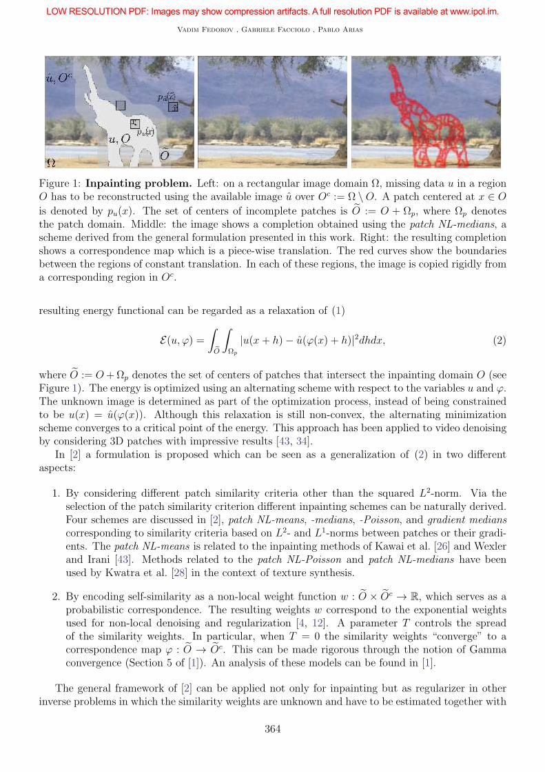
Figure 1: Inpainting problem. Left: on a rectangular image domain Ω, missing data u in a regionO has to be reconstructed using the available image u over Oc := Ω \O. A patch centered at x ∈ O

is denoted by pu(x). The set of centers of incomplete patches is O := O + Ωp, where Ωp denotesthe patch domain. Middle: the image shows a completion obtained using the patch NL-medians, ascheme derived from the general formulation presented in this work. Right: the resulting completionshows a correspondence map which is a piece-wise translation. The red curves show the boundariesbetween the regions of constant translation. In each of these regions, the image is copied rigidly froma corresponding region in Oc.

resulting energy functional can be regarded as a relaxation of (1)

E(u, ϕ) =∫

O

∫

Ωp

|u(x+ h)− u(ϕ(x) + h)|2dhdx, (2)

where O := O+Ωp denotes the set of centers of patches that intersect the inpainting domain O (seeFigure 1). The energy is optimized using an alternating scheme with respect to the variables u and ϕ.The unknown image is determined as part of the optimization process, instead of being constrainedto be u(x) = u(ϕ(x)). Although this relaxation is still non-convex, the alternating minimizationscheme converges to a critical point of the energy. This approach has been applied to video denoisingby considering 3D patches with impressive results [43, 34].

In [2] a formulation is proposed which can be seen as a generalization of (2) in two differentaspects:

1. By considering different patch similarity criteria other than the squared L2-norm. Via theselection of the patch similarity criterion different inpainting schemes can be naturally derived.Four schemes are discussed in [2], patch NL-means, -medians, -Poisson, and gradient medians

corresponding to similarity criteria based on L2- and L1-norms between patches or their gradi-ents. The patch NL-means is related to the inpainting methods of Kawai et al. [26] and Wexlerand Irani [43]. Methods related to the patch NL-Poisson and patch NL-medians have beenused by Kwatra et al. [28] in the context of texture synthesis.

2. By encoding self-similarity as a non-local weight function w : O × Oc → R, which serves as aprobabilistic correspondence. The resulting weights w correspond to the exponential weightsused for non-local denoising and regularization [4, 12]. A parameter T controls the spreadof the similarity weights. In particular, when T = 0 the similarity weights “converge” to acorrespondence map ϕ : O → Oc. This can be made rigorous through the notion of Gammaconvergence (Section 5 of [1]). An analysis of these models can be found in [1].

The general framework of [2] can be applied not only for inpainting but as regularizer in otherinverse problems in which the similarity weights are unknown and have to be estimated together with

364

Variational Framework for Non-Local Inpainting

the image ([21], [37], [36]). For the inpainting application it is best suited to take T = 0, becauseT > 0 implicates also denoising within the inpainting domain. Therefore, in this work we focus onthe case T = 0.

The inpainting is performed by an iterative minimization process, alternating between imageand correspondence map updates. This iterative process tends to generate a sort of patchwork ofsegments copied from the known portion of the image. An example is shown in Figure 1. Thetransition between copied segments takes place at a narrow band along the boundary between them.The four inpainting schemes differ in the way this transition is done (and in the partition found).Methods based on the L2-norm perform a smooth blending, whereas those based on the L1-normfavor sharper transitions.

In particular, patch NL-Poisson and patch NL-gradient medians combine the exemplar-basedinterpolation with PDE-based diffusion schemes. This results in a smoother continuation of theinformation across the boundary and inside the inpainting domain, and in a better propagation ofstructures. Furthermore, the inclusion of gradients in the patch similarity criterion allows to handleadditive brightness changes.

1.2 Contributions

This publication describes the implementation of the inpainting framework [2] for the case T = 0,providing a detailed description and C++ source code for three of the inpainting schemes derivedfrom it: patch NL-means, patch NL-medians and patch NL-Poisson. The code was designed so thatother inpainting schemes, derived from the same framework with different patch similarity criteria,can be easily added (such as the patch NL-gradient medians).

Although the code is written with more emphasis on readability than on performance, for thecomputation of the correspondence map we use a parallel version of the PatchMatch Algorithm [6],an efficient algorithm to approximate optimal correspondences.

After introducing the notation in the next subsection, in Section 2 we introduce the continuousvariational framework [2] and the inpainting energies derived from it. Section 3 focuses on the discretemultiscale minimization of these energies. The efficient computation of the patch correspondencesis done using the PatchMatch Algorithm [6], which is described in Section 3.3. Section 4 presentssome experiments and Section 2.3 some extensions of the framework. The organization of the codeis commented in Appendix A.

1.3 Notation

Images are denoted as functions u : Ω → R, where Ω denotes the image domain, a rectangle in R2.

We commonly refer to points in Ω as pixels and denote them by x, x, z, z. Positions inside the patchare denoted as y. A patch of u centered at x is denoted by pu(x) := pu(x, ·) : Ωp → R, where Ωp isa rectangle centered at 0. The patch is defined by pu(x, y) := u(x + y), with y ∈ Ωp. Let O ⊂ Ω bethe hole or inpainting domain, and Oc = Ω \ O. We assume that O is an open set with Lipschitzboundary. We still denote by u : Oc → R the known part of the image u: u := u|Oc .

We denote by Ω the set of centers of patches contained in the image domain, i.e. Ω = x ∈ Ω :

x + Ωp ⊆ Ω. As was defined in the Introduction, we take O as the set of centers of patches that

intersect the hole, i.e. O := O + Ωp = x ∈ Ω : (x + Ωp) ∩ O 6= ∅. For a simplified presentation,

we assume that O ⊆ Ω, i.e. every pixel in O is the center of a patch contained in Ω. We denoteOc = Ω \ O. Thus, patches pu(y) centered at points y ∈ Oc are contained in Oc (see Figure 1).Further notation will be introduced in the text.

365

Vadim Fedorov , Gabriele Facciolo , Pablo Arias

2 Variational Framework

Let us briefly review the inpainting framework proposed in [2] (we will focus here on the particularcase when T → 0, please refer to [2] for a more general presentation).

The image inpainting problem is posed as the minimization of the following energy

EE(u, ϕ) =∫

O

E(pu(x)− pu(ϕ(x)))dx, (3)

where E is a patch error function which measures patch similarity. Similarly to Equation (2), thisenergy forces every patch inside the inpainting domain O to be similar to some patch in Oc. Differentchoices of E yield different methods.

2.1 The Patch Error Function E

We consider [2] patch error functions E : Ωp → R+ defined either as the weighted sum of pixel errors

E(pu(x) − pu(x)) := g ∗ e(u(x + ·) − u(x + ·)) =

∫

Ωp

g(h)e(u(x + h) − u(x + h))dh,

where e : R→ R+, or gradient errors

E(pu(x) − pu(x)) := g ∗ e(∇u(x + ·) − ∇u(x + ·)) =

∫

Ωp

g(h)e(∇u(x + h) − ∇u(x + h))dh.

where e : R2 → R+. Here, g : R2 → R

+ denotes a suitable intra-patch kernel function, a nonne-

gative function such that∫g(h) dh = 1. For example the Gaussian weights g(h) = 1

Zexp (−‖h‖2

2a2),

with standard deviation a and normalization factor Z. We will consider three concrete patch errorfunctions.

Patch non-local means. In this case we use e(r) = |r|2 and the patch error function is a weightedsquared L2-norm that we denote by

E2(pu(x)− pu(x)) = ‖pu(x)− pu(x)‖2g,2 = g ∗ |u(x+ ·)− u(x+ ·)|2. (4)

Patch non-local medians. If we set e(r) = |r| then the patch error function results in a weightedL1-norm

E1(pu(x)− pu(x)) = ‖pu(x)− pu(x)‖g,1 = g ∗ |u(x+ ·)− u(x+ ·)|. (5)

Patch non-local Poisson. Taking a pixel error e( · ) that is a convex combination (with parameterλ ∈ [0, 1)) of intensity and gradient errors results in the following patch error function:

Eλ,2(pu(x)− pu(x)) = λ‖pu(x)− pu(x)‖2g,2 + (1− λ)‖pu(x)− pu(x)‖2g,2,∇ =

g ∗(λ|u(x+ ·)− u(x+ ·)|2 + (1− λ)|∇u(x+ ·)−∇u(x+ ·)|2

). (6)

Note that if we set λ = 1 we get E2.By plugging each of these patch error functions in the energy EE we get different inpainting

functionals. As it will be discussed below, the patch error function determines not only the similaritycriterion but also the image synthesis, thus it is a key element in the framework.

Additional patch error functions could be considered. For example in [2] the L1 norm betweenpatches of the gradient is also considered.

366

Variational Framework for Non-Local Inpainting

2.2 Minimization of the Energies

The objective EE in (3) is non-convex, and we can only compute a local minimum. To that aim, weuse an alternating minimization algorithm. At each iteration, two optimization steps are solved: theconstrained minimization of EE with respect to ϕ while keeping u fixed; and the minimization of EEwith respect to u with ϕ fixed. This procedure is detailed next and summarized in Algorithm 1.

Algorithm 1: Alternate minimization of EE(u, ϕ).input : Initial condition u0(x) with x ∈ O, tolerance τ > 0output: Inpainted image uk+1, offset map ϕk

repeat

ϕk ← argminϕEE(uk, ϕ). //§ 2.2.1: Correspondence update

uk+1 ←

argminu EE(u, ϕk) //§ 2.2.2: Image update: (11), (12), or (19)

subject to uk+1(x) = u(x), ∀x ∈ Oc

until ‖uk+1 − uk‖ < τ

2.2.1 Correspondence Update Step

When u is fixed, the minimization with respect to ϕ can be done independently for each x ∈ O. Thisamounts to determine the location in Oc of the most similar patch to pu(x), which is said to be thenearest neighbor of pu(x):

ϕ(x) ∈ argminx∈Oc

E(pu(x)− pu(x)). (7)

In Section 3.3 we describe an efficient way to compute the nearest neighbor for all the pixels in Owithout using an exhaustive search.

2.2.2 Image Update Step

Before moving to the derivation of the image update step for the different error functions: (4), (5),and (6), let us remark that with the change of variables z := x + h, z := x + h, the energy (3) canbe expressed as an accumulation of pixel errors

EE(u) =∫

O

∫

Ωp

g(h)e(u(x+ h)− u(ϕ(x) + h))dhdx =

∫

O

∫

Oc

m(z, z)e(u(z)− u(z))dzdz + C, (8)

where C is a constant term, and the pixel influence weights m : O ×Oc → R+ is defined as

m(z, z) =

∫

Ωp

g(h)χO(z − h)δϕ(z−h)(z − h)dh =

∫

Ωp

g(h)χO(z − h)δϕ(z−h)+h(z)dh. (9)

The characteristic function χO(x) (1 inside O and 0 otherwise) zeroes out the terms for which z − h

falls out of O, where ϕ is not defined.For each pair of pixels (z, z) ∈ O × Oc, m(z, z) weights the effective contribution of the pixel

error between u(z) and u(z) in the total value of the energy. The quantity m(z, z) is determined byintegrating the correspondences between all patches that overlap z and those that overlap z in thesame relative position (shown in Figure 2).

Let us also introduce the following notation, for z ∈ O:

k(z) :=

∫

Oc

m(z, z)dz, (10)

367

Vadim Fedorov , Gabriele Facciolo , Pablo Arias

Figure 2: Patch non-local inpainting. The value at z ∈ O is computed using contributions fromall the patches that overlap it, i.e. those centered at x ∈ O such that z = x + h with h ∈ Ωp. Theinfluence function m(z, z) accounts for the contributions from patches centered at z − h to z − h.

Since g is normalized, we have that k(z) = 1 for all z ∈ O. Thus, m(z, ·) can be interpreted as aprobability density function. Later on, we will consider confidence weights for which k(z) 6= 1. Forthis reason we will keep the notation k(z) in the following derivations.

Patch non-local means. Taking the weighted squared L2-norm ‖pu(x)−pu(x)‖2g,2 as a patch errorfunction (4), the energy (8) becomes quadratic on u. Thus its minimum for a fixed correspondenceϕ can be computed explicitly as a non-local average of the known pixels:

u(z) =1

k(z)

∫

Oc

m(z, z)u(z)dz, (11)

for z ∈ O. By expanding m we note that each patch overlapping z contributes a value for the currentpixel z

u(z) =1

k(z)

∫

Ωp

g(h)u(ϕ(z − h) + h)dh.

Patch non-local medians. Considering the L1-norm patch error function (5), corresponds totaking e(x) = |x| in (8). The Euler equation for u can be formally written as

[δuEE(u)](z) =∫

Oc

sign[u(z)− u(z)]m(z, z)dz ∋ 0. (12)

This expression is multivalued, since sign(r) := r/|r| if |r| > 0 and sign(r) ∈ [−1, 1] if r = 0. Itssolution u(z) for every z ∈ O is obtained as a weighted median of the pixels of the complement Oc,with weights m(z, · ).

Both schemes presented so far perform inpainting by transferring (averages or medians) knowngray levels into the inpainting domain. As we will see next, using a patch error function based onthe gradient of the image yields a method that transfers gradients and computes the resulting imageas the solution of a PDE. This results in better continuation properties of the solution, in particularat the boundary of the inpainting domain.

Patch non-local Poisson. The patch NL-Poisson combines weighted L2-norms of intensity (5)and gradients (6). The resulting energy is

Eλ,2(u) =∫

O

∫

Oc

m(z, z)[(1− λ)|∇u(z)−∇u(z)|2 + λ(u(z)− u(z))2]dzdz. (13)

368

Variational Framework for Non-Local Inpainting

Note that (13) can be rewritten as

Eλ,2(u) ∝∫

O

k(z)|∇u(z)− v(z)|2dz + λ

1− λ

∫

O

k(z)(u(z)− f(z))2dz + C, (14)

where C is a constant term,

f(z) :=1

k(z)

∫

Oc

m(z, z)u(z)dz (15)

is the solution of the patch NL-means image update step, and the field v : O → RN is given by

v(z) :=1

k(z)

∫

Oc

m(z, z)∇u(z)dz. (16)

This energy balances two terms. The first one imposes the gradients of u to be close (in the L2

sense) to a guiding vector field v computed as a non-local weighted average of the image gradientsin the known portion of the image. The second term corresponds to a quadratic attachment to thesolution of the patch NL-means image update.

In this case the Euler-Lagrange equation w.r.t. u is the screened Poisson equation

div[k(z)∇u(z)] − λ

(1− λ)k(z)u(z) =

div[k(z)v(z)] − λ

(1− λ)k(z)f(z), z ∈ O,

u(z) = u(z), z ∈ ∂O \ ∂Ω,∇u(z) · nΩ(z) = 0, z ∈ ∂O ∩ ∂Ω.

(17)

Here nΩ(z) ∈ RN denotes the outgoing normal to Ω, for z ∈ ∂Ω. The problem is linear and in a

discrete setting it can be solved for instance with a conjugate gradient algorithm.When λ = 0 the attachment to f vanishes and only gradients are transfered to the inpainting

domain, the resulting PDE is a Poisson equation. In this case, the patch similarity (that determinesm) is computed based solely on the gradients. However, the gradient is usually not a good featurefor measuring the patch similarity, and it is convenient to consider also the gray level/color data.Typically we will set λ 6 0.1, in this way some intensity information is included in the computationof the correspondences, without departing too much from the Poisson equation.

2.3 Extension: Decoupling Image and Correspondence Update Steps

In the variational setting, the image synthesis and the correspondence update are coupled througha unique patch error function E. One can envision a broader family of (non-variational) methodsin which different patch comparison criterions can be chosen independently for the correspondenceupdate step and for the image update step. If we denote by Eu and Eϕ the patch error functions forimage update and the correspondence update respectively, we have the following algorithm (Algo-rithm 2).

This is useful in practice for gradient-based methods. Gradient-based methods produce smoothinterpolations and enforce the continuity of the image at the boundary of the inpainting domain,which are generally desirable features. For this to be done variationally the correspondences ϕ have tobe computed using patches of the gradient, which in most cases do not provide a reliable measure ofpatch similarity. For this reason for patch NL-Poisson we define the patch error function as a convexcombination between a gradient patch error function and the squared L2-norm of intensities (thepatch error function of patch NL-means). In this way, by controlling the coefficient λ of the convex

369

Vadim Fedorov , Gabriele Facciolo , Pablo Arias

Algorithm 2: Alternate minimization of EEuand EEϕ

.

Initialization: choose u0 with ‖u0‖∞ ≤ ‖u‖∞.for k ∈ N do

ϕk+1 ← argminϕEEϕ

(uk, ϕ);

uk+1 ← argminuEEu

(u, ϕk+1);

combination we can take the image values into account for the computation of the correspondences,and at the same time, to synthesize the image with a diffusion PDE.

However, in many cases, one cannot find a value of λ which balances a gradient-based blending ofthe image and at the same time produces reliable correspondences. For such cases it is useful to extendgradient-based methods by considering two mixture coefficients: λϕ ∈ [0, 1] for the correspondencesupdate step and λu ∈ [0, 1] controlling the image synthesis. This allows to combine the benefits ofintensity- and gradient-based methods into a single algorithm.

3 Implementation

In this section we describe the main implementation aspects of the schemes presented in the previoussection. Section 3.2 details the implementation of the different image update steps. Section 3.3 isdevoted to the update of the correspondence map (or nearest neighbor field), for what we use thePatchMatch Algorithm [6], which permits to efficiently compute an approximate nearest neighborfield. Finally, in Section 3.4 we describe a multiscale scheme, necessary to avoid bad local minima.

3.1 Discrete Setting and Notation

Throughout this section we consider discrete images defined over a rectangular bounded domain Ω :=0, . . . , N2 and corresponding discrete versions of the inpainting domain O and its complement Oc.To avoid a cumbersome notation, we slightly modify it in this section (for instance some argumentsof functions will be denoted as subindices). The discrete energy reads

EE(u, ϕ) =∑

x∈O

E(pu(x)− pu(ϕ(x))). (18)

Patches are now functions defined on a discrete domain Ωp. The patch error function E is definedas the weighted sum of pixel errors

E(pu(x)− pu(x)) =∑

h∈Ωp

ghe(ux+h − ux+h),

where e : R→ R+, or gradient errors

E(pu(x)− pu(x)) =∑

h∈Ωp

ghe(∇ux+h −∇uy+h),

where e : R2 → R+. Here, g : Z2 → R

+ denotes the intra-patch kernel function, which is nonnegative,with support Ωp and

∑h∈Z2 gh = 1.

We need to define the discrete version of the gradient and divergence operators. We will use thenotation [A→ B] = f : A→ B, the set of functions from A to B.

370

Variational Framework for Non-Local Inpainting

We define ∇ : [Ω→ R]→ [Ω→ R2] as

∇u1i,j :=

0 if i = N ,ui+1,j − ui,j if i < N ,

and similarly for the component ∇u2i,j. The notation z = (i, j) refers to locations on the image. Let

us also define a divergence operator ∇· : [Ω→ R2]→ [Ω→ R],

∇ · pi,j :=

p1i,j if i = 0,−p1i−1,j if i = N ,p1i,j − p1i−1,j otherwise,

+

p2i,j if j = 0,−p2i,j−1 if j = N ,p2i,j − p2i,j−1 otherwise.

These operators incorporate Neumann boundary conditions on the boundary of Ω, and are dualoperators, i.e. denoting 〈·, ·〉 the usual scalar products in [Ω→ R] and [Ω→ R

2], 〈∇u, p〉 = −〈u,∇·p〉,for all u ∈ [Ω→ R], p ∈ [Ω→ R

2].

3.2 Image Update Step

For the computation of the image update step, we will rewrite the energy using the pixel influenceweights m : Oe ×Oc

e → R+

mzz =∑

h∈Ωp

ghδϕ(z−h)(z − h)χO(z − h).

Correspondingly we also define the normalization factor kz :=∑

z∈Oc mzz.

Patch NL-means and patch NL-Poisson. The discrete version of the patch NL-Poisson energyis given by

Eλ,2(u) =∑

z∈Oe

∑

z∈Oce

mzz[(1− λ)|∇uz −∇uz|2 + λ(uz − uz)2].

The energy is quadratic in u and can be minimized by solving the following linear equation:

(1− λ)∇ · [kz∇uz]− λkzuz = (1− λ)∇ · [kzvz]− λkzfz, z ∈ Oe,u(z) = u(z), z ∈ Oe \O,

(19)

where we have defined

fz :=1

kz

∑

z∈Oce

mzzuz and vz :=1

kz

∑

z∈Oce

mzz∇uz.

Equation (19) can be solved efficiently with a conjugate gradient Algorithm [40].When λ = 1, we recover the NL-means case and the solution can be computed directly as uz = fz.

Patch NL-medians. The discrete version of the patch NL-medians energy is given by

E1(u) =∑

z∈O

∑

z∈Oc

mzz|uz − uz|.

This problem can be solved for each z independently, and its solution is given by a weighted median(with weights mzz) of the known values uz. To compute the weighted median the values uz are firstsorted, then the vector is traversed while accumulating the weights, the median corresponds to theelement for which the accumulator attains half of the total weight.

371

Vadim Fedorov , Gabriele Facciolo , Pablo Arias

Algorithm 3: PatchMatch

input : image u, inpainting domain O, target image u, I iterationsoutput: offset field θ // can be converted to correspondences: ϕx = x+ θx

θ ←− Randomly initialize the entire offset map

(xn), n = 1, . . . , |O| ←− Raster ordering of the pixels in O

for iter = 0, . . . , I − 1 do

for n = 0, . . . , |O| − 1 do

// Offset propagation

if (iter mod 2) = 0 then

x = (i, j)←− xn

T←− θi,j , θi,j−1 , θi−1,j // candidate offsets for raster (up and left)

else

x = (i, j)←− x|O|−n

T←− θi,j , θi,j+1 , θi+1,j // candidate offsets for inverse raster (down and right)

θx ←− argmint∈T

E(pu(x)− pu(x+ t)) // keep the offset yielding the minimum error

// Random search

S←− Generate set of random offsets around θx // according to (21)

θx ←− argmint∈θx∪ S

E(pu(x)− pu(x+ t))

3.3 PatchMatch for Computing the Nearest Neighbor Field

The updating of correspondences is the most time consuming step in the minimization of the in-painting energies (Algorithm 1). A brute force search for correspondences requires O(|O||Oc||Ωp|)operations. In this section we describe (see Algorithm 3) the PatchMatch algorithm [6], which effi-ciently finds an approximate solution to this problem. Following [6], let us express the correspondencemap as offsets θx = ϕx − x ∈ Z

2. We need to solve the following problem:

θx ∈ argmint∈Z2 :x+t∈Oc

e

E(pu(x)− pu(x+ t)), for all x ∈ Oe. (20)

Although the patch error does not have to be a metric, we refer to pu(x+ θx) as the nearest patch or

nearest neighbor of pu(x), and to the offset map θ : O → Oc as the nearest neighbor field (NNF).

The search for the nearest neighbor is performed simultaneously over all the points in O basedon the following heuristic: since query patches overlap, the offset θx of a good match at x is likely tobe a good match for points close to x.

PatchMatch is an iterative algorithm which starts from a random initialization, when each pixelx in the extended inpainting domain O is associated with a candidate correspondence ϕx ∈ Oc

following a uniform distribution over Oc. The corresponding offset is then θx = ϕx − x. After theinitialization, each iteration goes through all pixels in O and performs two operations at each pixel:offsets propagation and random search. In odd iterations, pixels are traversed in raster order (fromleft to right, top to bottom), while in even iterations the inverse ordering is used.

372

Variational Framework for Non-Local Inpainting

Figure 3: Steps of the PatchMatch algorithm: a) assign offsets at random; b) check left and topneighbors of the blue patch for the better offset (suppose iteration is odd); c) search for the betteroffsets at random in sequentially decreasing windows.

Offsets propagation. Let us consider an odd iteration, when pixels are traversed in raster order.At the pixel x = (i, j), the offsets of its left and top neighbors are tested as candidate offsets forx. Among θi,j, θi−1,j and θi,j−1, the offset yielding the least patch error is kept as candidate. Notethat the left and top neighbors have already been visited in the propagation scan. In a backwardpropagation step the pixels are traversed in the inverse order. Correspondingly, when visiting a pixel,we consider the offsets from its right and bottom neighbors.

Random search. The result of the propagation is refined with a random search that samples aset of candidate offsets for the pixel x. The patch error of each one of these candidate offsets iscompared with the current offset θx, and the one with minimum error is kept. Each sample ti ∈ Z

2,i = 0, 1, . . . is drawn from a uniform distribution in a square neighborhood centered at the currentoffset, i.e.

ti ∼ U([−αiNmax, αiNmax]

2) + θx. (21)

Here Nmax is the maximum image dimension and α = 1/2. Each sample is taken from a smallerwindow until the sampling window becomes smaller that 3 × 3 pixels. This ensures that offsetsclose to the current candidate are more densely sampled. Taking Nmax as the largest image dimen-sion guarantees that all the image can be sampled with non-zero probability, which guarantees theasymptotic convergence of the algorithm to the true NNF.

The computational cost of one PatchMatch iteration (random search and propagation) isO(|Ωp||O|),whereas the memory requirements are of O(|O|). For most applications, a few iterations are oftensufficient. See [6] and [7] for more details about the PatchMatch algorithm and some generalizations,and see [1] for an analysis of its convergence rate.

3.3.1 Parallelization of PatchMatch

Parallelization might be used to further accelerate the nearest neighbor field estimation with Patch-Match. In [6] it was proposed to implement PatchMatch on a GPU using the jump flood algorithmof [39] to accelerate the propagation step. Here, we focus on the parallelization for CPU consideringseveral options.

373

Vadim Fedorov , Gabriele Facciolo , Pablo Arias

Algorithm 4: PatchMatch parallelization with decoupling

. . .for iter = 0, . . . , I − 1 do

// Offset propagation (raster or inverse raster order)

for n = 0, . . . , |O| − 1 do

Propagate at pixel n . . .

// Random search. The following loop is parallel

parallel for n = 0, . . . , |O| − 1 do

Random search at pixel n . . .

Note in Algorithm 3 that at a given pixel the propagation step is immediately followed by therandom search. The loops cannot be parallelized naively because the propagation is sequential: itdepends on the preceding neighbors according to the propagation order. One approach would be todecouple the propagation and search steps as in Algorithm 4: the propagation is done first for allpixels and then the random search is performed on all pixels. In this way, all data dependencies areleft in the propagation step and the search step can be easily parallelized. However, such decouplingslows down the propagation of good random offsets, therefore it affects the convergence speed (thatis, to attain a similar result, Algorithm 4 may require more iterations than Algorithm 3).

A slightly different approach to parallelization considers the pixels diagonal-by-diagonal (goingfrom the top-right to the bottom-left corner of the image) instead of the usual row-by-row. Inthis way, during the propagation step (on odd iterations), each pixel depends only on its top andleft neighbors (or bottom and right neighbors on even iterations). This means, that pixels in thesame diagonal are independent during both propagation and search steps, hence can be processedin parallel. This algorithm yields exactly the same result as Algorithm 3. However, since it violatesthe data locality principle, in practice it has a poor performance because of the reduced efficiency ofdata caching in the CPUs.

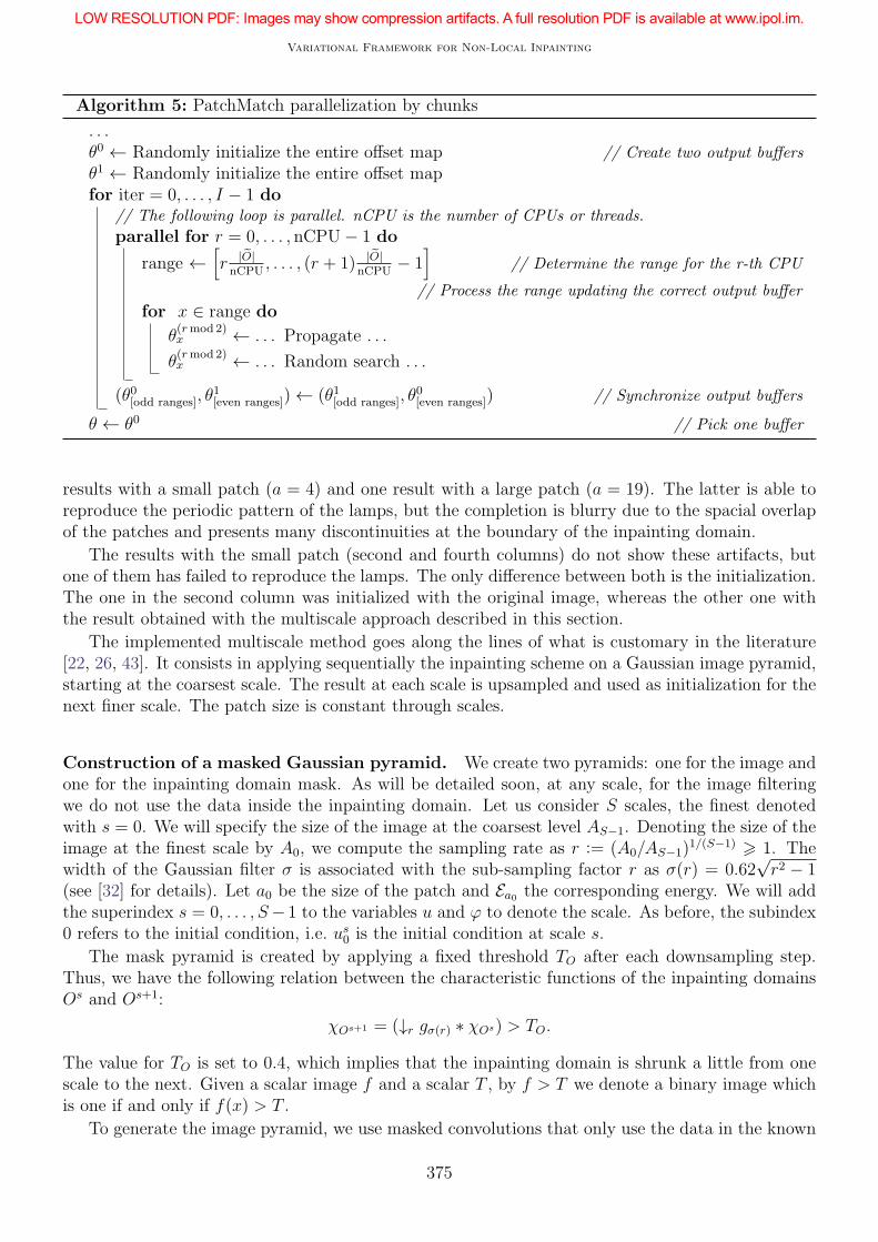
In this work we implement a parallelization scheme, mentioned in [7]. Assuming that P CPUsare available, we split the inpainting domain in chunks of equal sizes. In each iteration propagationand random search are performed independently for each chunk on a separate processor, as detailedin Algorithm 5. Each chunk consists of |O|/P pixels of the inpainting domain. In a row-by-rowrepresentation of an image each processor gets some adjacent rows. In this way, within a single iter-ation, a good offset cannot be propagated across chunks. To allow propagation across the boundaryof a chunk we use two separate buffers for odd and even chunks and after each iteration we copythe boundary rows from one buffer to another. As a drawback, this scheme affects the convergencespeed due to the limited propagation, however, to our knowledge this effect is negligible.

3.4 Multiscale Scheme

As in many state of the art exemplar-based inpainting methods (e.g. [26, 27, 43]), we incorporate amultiscale scheme. As noted in [24] and, as the example of Figure 4 suggests, inpainting is inherentlya multiscale problem: images have structures of different sizes, ranging from large objects (as thelamps and their periodic distribution on the image) to fine scale textures (like the characters) andedges. The multiscale scheme responds to the fact that several patch sizes are needed to reproduceall these structures properly.

In Figure 4, we show completions obtained with patch NL-means using different patch sizes.We used a Gaussian intra-patch weight kernel g with standard deviation a. The figure shows two

374

Variational Framework for Non-Local Inpainting

Algorithm 5: PatchMatch parallelization by chunks

. . .θ0 ← Randomly initialize the entire offset map // Create two output buffers

θ1 ← Randomly initialize the entire offset mapfor iter = 0, . . . , I − 1 do

// The following loop is parallel. nCPU is the number of CPUs or threads.

parallel for r = 0, . . . , nCPU− 1 do

range ←[r |O|nCPU

, . . . , (r + 1) |O|nCPU

− 1]

// Determine the range for the r-th CPU

// Process the range updating the correct output buffer

for x ∈ range do

θ(rmod 2)x ← . . . Propagate . . .

θ(rmod 2)x ← . . . Random search . . .

(θ0[odd ranges], θ1[even ranges])← (θ1[odd ranges], θ

0[even ranges]) // Synchronize output buffers

θ ← θ0 // Pick one buffer

results with a small patch (a = 4) and one result with a large patch (a = 19). The latter is able toreproduce the periodic pattern of the lamps, but the completion is blurry due to the spacial overlapof the patches and presents many discontinuities at the boundary of the inpainting domain.

The results with the small patch (second and fourth columns) do not show these artifacts, butone of them has failed to reproduce the lamps. The only difference between both is the initialization.The one in the second column was initialized with the original image, whereas the other one withthe result obtained with the multiscale approach described in this section.

The implemented multiscale method goes along the lines of what is customary in the literature[22, 26, 43]. It consists in applying sequentially the inpainting scheme on a Gaussian image pyramid,starting at the coarsest scale. The result at each scale is upsampled and used as initialization for thenext finer scale. The patch size is constant through scales.

Construction of a masked Gaussian pyramid. We create two pyramids: one for the image andone for the inpainting domain mask. As will be detailed soon, at any scale, for the image filteringwe do not use the data inside the inpainting domain. Let us consider S scales, the finest denotedwith s = 0. We will specify the size of the image at the coarsest level AS−1. Denoting the size of theimage at the finest scale by A0, we compute the sampling rate as r := (A0/AS−1)

1/(S−1) > 1. Thewidth of the Gaussian filter σ is associated with the sub-sampling factor r as σ(r) = 0.62

√r2 − 1

(see [32] for details). Let a0 be the size of the patch and Ea0 the corresponding energy. We will addthe superindex s = 0, . . . , S− 1 to the variables u and ϕ to denote the scale. As before, the subindex0 refers to the initial condition, i.e. us

0 is the initial condition at scale s.

The mask pyramid is created by applying a fixed threshold TO after each downsampling step.Thus, we have the following relation between the characteristic functions of the inpainting domainsOs and Os+1:

χOs+1 = (↓r gσ(r) ∗ χOs) > TO.

The value for TO is set to 0.4, which implies that the inpainting domain is shrunk a little from onescale to the next. Given a scalar image f and a scalar T , by f > T we denote a binary image whichis one if and only if f(x) > T .

To generate the image pyramid, we use masked convolutions that only use the data in the known

375

Vadim Fedorov , Gabriele Facciolo , Pablo Arias

Figure 4: Single scale vs. multiscale. Left column: inpainting domain and initial condition. Forthe rest of the columns, from left to right: single scale inpainting with a 9 × 9 patch with a = 4;single scale inpainting with a 43 × 43 patch with a = 19; multiscale inpainting with three scales,corresponding to patch sizes of 9× 9 with a = 4, 21× 21 with a = 9, and 43× 43 with a = 19. Allresults have been computed with the patch NL-means scheme. The bottom row shows the boundariesbetween copy regions superimposed over the energy density image.

part of the image. At scale s, we have that

us+10 =↓r masked-convolution(gσ(r), (O

s)c; us),

The masked convolution operator, is defined for images g and f and a region A, as

masked-convolution(g, A; f)(x) =

∑h∈Z2 g(x− h)χA(h)f(h)∑

h∈Z2 g(x− h)χA(h)=

g ∗ (χAf)(x)

g ∗ χA(x).

In other words, the image at scale s is multiplied by the mask of known data before the convolutionwith the smoothing kernel. Afterwards a normalization is applied to each pixel.

Joint image and NNF upscaling. When going from scale s+ 1 to s we need to upsample boththe correspondence map and the inpainted image. We proceed as in [43]. The coarse correspondencesϕs+1 are first interpolated to the finer image size, yielding ↑r ϕs+1. For this we use nearest neighborinterpolation. These interpolated correspondences are then scaled by r, yielding ϕs

0 = r · ↑r ϕs+1.The image is upsampled by solving an image update step at the finer scale, using the upsampledcorrespondences: us

0 = minu Ea0(u, ϕs0). More conventional upsampling schemes by local interpolation

(such as bilinear or splines) introduce a bias towards low-frequency non-textured regions. Thisexemplar-based upsampling avoids such bias.

Notice that keeping the patch size constant while filtering and reducing the image can be seenas the sequential minimization of a series of inpainting energies with varying patch size given byas = (1/rs)a0, s = 0, . . . , S − 1, over a corresponding series of filtered images. In the coarsestscale S − 1, a larger portion of the inpainting domain is covered by partially known patches. Thismakes the inpainting task easier and less dependent on the initialization. The energy at this scaleshould have fewer local minima. The dependency of the minimization process on the initial conditionensures that each single scale solution remains close to the coarse scale initialization. The multiscalealgorithm exploits this dependency to obtain an image u0 which is approximately self-similar for allscales (or equivalently, for all patch sizes).

Figure 4 shows a comparison between single and multiscale results with the patch NL-meansscheme. The multiscale result shows the benefits of large and small patch sizes. The missing lamps

376

Variational Framework for Non-Local Inpainting

Algorithm 6: Multiscale inpainting scheme

input : known image u0, inpainting domain O, patch size a0, number of scales S, size ofcoarsest scale AS−1

output: inpainted image us and offset map ϕs at each scale

r ← (size(u0)/AS−1)1/(S−1) // size factor

Oss=0,...,S−1 ← Compute pyramid of domains (S scales, factor r) from Ous

0s=0,...,S−1 ← Initialize pyramid of images (S scales, factor r) from u0 and O

for s = S − 2, . . . , 0 do

if s = S − 1 then

us0 ← Initialize inpainting domain with average value of u0 in Oc

else

ϕs0 ← r · (↑r ϕs+1) // upsample using nearest neighbor interpolation and scale by r

us0 ← argminu Ea0(u, ϕs

0) // solve image update (§3.2)s.t. u(x) = us

0(x), ∀x 6∈ Os

(us, ϕs)← argmin(u,ϕ) Ea0(u, ϕ) // call to Algorithm 1

s.t. u(x) = us0(x), ∀x 6∈ Os,

with initial condition us0 in Os

have been completed with the correct shape and spacing by the coarser stages, and the fine details areoverall much less blurry. Also, there are almost no discontinuities at the boundary of O. The bottomrow shows the copy regions. The single scale results show a coarse partition for the large patch (thecopying is more rigid), and one with many small regions for the smaller patch. The multiscale NNFshows an intermediate partition, with some large regions inside of the hole and smaller ones aroundits boundary. The inpainting at the finer scales works by refining the coarse partition obtained atcoarser scales.

3.5 Confidence Mask

For large inpainting domains, it is useful to introduce a mask κ : Ω→ (0, 1] which assigns a confidencevalue to each pixel, depending on the certainty of its information (see also [16, 27]). This helps inguiding the flow of information from the boundary towards the interior of the hole, eliminating somelocal minima and reducing the effect of the initial condition. The resulting energy takes the form

EE(u, ϕ) =∑

x∈O

κ(x)E(pu(x)− pu(ϕ(x))). (22)

The effect of κ on the image update step can be seen on the pixel influence weights m

mzz =∑

h∈Ωp

ghκ(z − h)δϕ(z−h)(z − h)χO(z − h).

Thus, the contribution of the patch pu(z − y) to the evidence function is now weighted by its confi-dence. Patches with higher confidence will have a stronger influence.

377

Vadim Fedorov , Gabriele Facciolo , Pablo Arias

For the experiments shown in this paper, the confidence mask was set to

κ(x) =

(1− c0) exp

(−d(x,∂O)

tc

)+ c0 if x ∈ O,

1 if x ∈ Oc,

which shows an exponential decay w.r.t. the distance to the boundary inside the inpainting domaind(·, ∂O). Here tc > 0 is the decay time and c0 > 0 determines the asymptotic value reached far awayfrom the boundary. Setting tc = 0 results in a constant confidence mask.

3.6 Color Images

Energies for color images are obtained by defining a patch error function for color patches as the sumof the error functions of the three scalar components

E(pu(x)− pu(x)) =3∑

i=1

E(pui(x)− pui

(x)),

where u : Ω → R3 is the color image, and ui (with i = 1, 2, 3) are its components (analogously for

gradient-based errors). Given the correspondences, each channel is updated using the scheme forscalar images. All channels are updated using the same correspondences.

4 Experiments and Parameter Selection

In this section we demonstrate the proposed schemes on real inpainting problems and compare themwith four representative state of the art methods. The images used were obtained from [27] andfrom the inpainting benchmark proposed by [26], available at http://yokoya.naist.jp/research/inpainting/.

4.1 Experimental Setting

We consider three inpainting methods, variations of our proposed framework, namely patch NL-means, -medians and -Poisson. In all cases we use the multiscale approach and the CIELab colorspace.

Some representative results are shown in Figure 5. Obtaining good results requires fixing thefollowing parameters (see Table 1 for the concrete values used in the experiments):

Patch size. We used square patches with constant intra-patch weights (g = 1/|Ωp|). Gaussian-weighted patches require a larger support, reducing the available exemplars.

Multiscale parameters. The multiscale scheme has two parameters: the size of the coarsest imageAS−1 and the number of scales S. The former is the most critical one. We specify AS−1 as apercentage of the original size. The default value is set according to [34, 33], where it is notedthat the size of the inpainting domain in the coarsest scale should be smaller than twice thepatch size. In our implementation, the default value for AS−1 is

AS−1 =1.5 · patch size

maxx∈O d(x,Oc).

This default value can be overridden by the user. A reasonable initial guess for the number ofscales S can be such that the subsampling rate r = (A0/AS−1)

1/(S−1) ≈ 21/3 ≈ 1/0.8 as in [43].

378

Variational Framework for Non-Local Inpainting

Matsuri Mailboxes Baseball SofaM Md P M Md P M Md P M Md P

S 10 10 11 7 7 7 6 6 6 8 6 8AS−1,(%) 15 10 10 30 50 30 30 30 30 20 50 20patch size 7 7 7 9 11 9 9 9 7 11 11 7

tc 5 3 5 5 3 4 5 5 5 5 5 3λ – – 0.01 – – 0.05 – – 0.01 – – 0.01

Table 1: Parameters for the results on the images in Figures 4 and 5.

Confidence mask. The confidence mask has two parameters, the asymptotic value c0 and the decaytime tc. For all experiments we fix c0 = 0.1.

Initialization. To initialize the inpainting domain in the coarsest scale, we used a (local) Poissoninterpolation by solving ∆u(x) = 0 with Dirichlet boundary conditions.

Mixing coefficient. For the patch NL-Poisson scheme the mixing coefficient λ should be specifiedas well. Recall that lower values of λ give a higher weight to the gradient component of theenergy. This is appropriate for structured images with strong edges.

For the sake of comparison we also include results obtained using four representative methodsfrom the state of the art. Two of them compute a coarse correspondence map, the PatchWorks (PW)method [35] and the approach of [27] (KT). The first one is greedy and the latter is iterative. Seamsbetween blocks are eliminated a posteriori, using for instance a Poisson blending. The other twomethods compute a dense correspondence map: Resynthetizer (R) [23] (greedy) and the approachof [26] (KSY) (iterative). The latter is similar to the patch NL-means, with two improvements:locality of the nearest neighbor search and a correction that accounts for multiplicative brightnesschanges.

The results from KT were published in [27] and those from KSY can be found in [26] and arealso available at http://yokoya.naist.jp/research/inpainting/. The Resynthetizer algorithm isimplemented as a plug-in for the GIMP image editing software2. Our implementation of PatchWorkswas written by Geoffrey Scoutheeten and was kindly made available to us by Simon Masnou. It doesnot include the blending post-processing step, so all seams are visible. We refer the reader to [35]and [13] for results obtained using this efficient technique with blending.

The three inpainting schemes presented here differ in the way the patches are blended. Methodsbased on the L2-norm perform a smooth blending, whereas those based on the L1-norm favor sharpertransitions.

It is notorious that patch NL-medians performs better at reproducing fine textures (Figure 5b).The results of the L2 methods are smoothed by the spatial averaging of overlapping patches. Onthe other hand, patch NL-medians creates sharp discontinuities when different copy regions meet(Figure 5c). These discontinuities are very noticeable and in these cases some smoothing is desirable.Also patch NL-medians generally requires the use of larger patches, particularly for structured images.

Patch NL-Poisson combines the exemplar-based interpolation with PDE-based diffusion schemes.This results in a smoother continuation of the information across the boundary and inside the in-painting domain, and in a better propagation of structures (Figures 5c and 5a). Furthermore, theinclusion of gradients in the patch similarity criterion allows to handle additive brightness changes.

2GIMP: GNU Image Manipulation Program. S. Kimball, P. Mattis and the GIMP Dev. Team. http://www.gimp.org/. Version 2.6.8 released on December 2009.

379

Vadim Fedorov , Gabriele Facciolo , Pablo Arias

(a) Example with periodic textures (Mailboxes)

(b) Example with random textures (Baseball)

(c) Example with structures (Sofa)

Figure 5: Results on periodic, textured, and structured images. PW: PatchWorks [35], R:Resynthesizer [23] ,KT: method of [27], and KSY: Kawai et al. [26]. M, Md and P stand for patchNL-means, -medians and -Poisson.

380

Variational Framework for Non-Local Inpainting

This is not the case for intensity-based methods (patch NL-means and NL-medians), which produceabrupt transitions at the boundary of the hole and between copy regions (Figures 5a and 5c).

A Organization of the Code

In this section we briefly describe the architecture of the code. The provided implementation iswritten in C++ and is object oriented, so the algorithm is encapsulated in a number of classes,which can be divided into data structures, algorithms, and utilities. The code was designed to bemodular so that these new schemes can be added easily: only the patch similarity criterion and thecorresponding image update step need to be implemented.

Although the code is written with more emphasis on readability than on performance, for thecomputation of the correspondence map we implemented a parallel version of PatchMatch [6].

A.1 Data Structures

These classes were designed to store the data:

Shape: container for a 2D rectangular shape (width and height).

Image: container for an image with some defined pixel type.

Mask: container for a binary mask. Mask differs from image in that it provides methods to iterateover the region represented by the mask.

A.2 Algorithms

These are the main classes that encapsulate the logic of the inpainting algorithms:

ImageInpainting: the main class implementing the image inpainting method. It should be param-eterized by the PatchMatch class and a class derived from AImageUpdating.

PatchMatch: implementation of the Patch-Match algorithm. It should be parameterized by a classderived from APatchDistance.

APatchDistance: abstract base class for different patch distances. We have implemented thefollowing patch distances, derived from APatchDistance:

L2NormPatchDistance: implementation of the L2-Norm patch distance.

L1NormPatchDistance: implementation of the L1-Norm patch distance.

L2CombinedPatchDistance: implementation of the L2-Norm patch distance which takesinto account intensity differences and gradient differences. The relative importance of theintensity term over the gradient term is controlled by the ‘lambda’ parameter.

AImageUpdating: abstract base class for different image updating methods. We have implementedthe following image update methods, derived from AImageUpdating:

PatchNonLocalPoisson: implementation of the Non-Local Poisson image updating scheme.

PatchNonLocalMeans: implementation of the Non-Local Means image updating scheme.

PatchNonLocalMedians: implementation of the Non-Local Medians image updating scheme.

Abstract APatchDistance and AImageUpdating classes with their corresponding derived classesallow to easily configure the algorithm to apply any desired approach (NL-means, NL-Poisson, etc.).The following example shows how they are used.

381

Vadim Fedorov , Gabriele Facciolo , Pablo Arias

A.2.1 Usage Example

Setup Image inpainting algorithm.

// setup patchmatch

Shape patch size = Shape(patch_side , patch_side );

APatchDistance *patch distance = new L2CombinedPatchDistance(lambda ,

patch size, patch_sigma );

PatchMatch *patch match = new PatchMatch(patch distance,

patch_match_iterations , random_shots_limit , -1);

// setup image update

AImageUpdating *image updating = new PatchNonLocalPoisson(patch size, patch_sigma ,

lambda , conj_grad_tol , conj_grad_iter );

// create inpainting object

ImageInpainting image inpainting = ImageInpainting(inpainting_iterations ,

tolerance ,

scales_amount ,

subsampling_rate ,

confidence_decay_time ,

confidence_asymptotic_value ,

initialization_type ); // enum

image inpainting.set weights updating(patch match);

image inpainting.set image updating(image updating);

Call the algorithm.

// image of type Image , and mask of type Mask

Image<float > output = image inpainting.process(input , mask);

The implementation can be extended to new inpainting schemes corresponding to different patchsimilarity criteria. To do so, one needs to implement only the image update class and the patchdistance class.

Acknowledgment

Work partly founded by the Centre National d’Etudes Spatiales (CNES, MISS Project), BPIFranceand Rgion Ile de France, in the framework of the FUI 18 Plein Phare project, the European ResearchCouncil (advanced grant Twelve Labours 246961), and the Office of Naval research (ONR grantN00014-14-1-0023).

Image Credits

The Berkeley Segmentation Dataset and Benchmark3

The Berkeley Segmentation Dataset and Benchmark 3

The Berkeley Segmentation Dataset and Benchmark 4

Norihiko Kawai [26], Evaluation for Image Inpainting image No. 0575

3http://www.eecs.berkeley.edu/Research/Projects/CS/vision/grouping/segbench/5http://yokoya.naist.jp/research/inpainting/

382

Variational Framework for Non-Local Inpainting

Norihiko Kawai [26], Evaluation for Image Inpainting image No. 0785

References

[1] P. Arias, V. Caselles, and G. Facciolo, Analysis of a variational framework for exemplar-

based image inpainting, Multiscale Modeling & Simulation, 10 (2012), pp. 473–514. http:

//dx.doi.org/10.1137/110848281.

[2] P. Arias, G. Facciolo, V. Caselles, and G. Sapiro, A variational framework for

exemplar-based image inpainting, International Journal of Computer Vision, 93 (2011), pp. 319–347. http://dx.doi.org/10.1007/s11263-010-0418-7.

[3] J.-F. Aujol, S. Ladjal, and S. Masnou, Exemplar-based inpainting from a variational

point of view, SIAM Journal of Mathematical Analysis, 42 (2010), pp. 1246–1285. http://dx.doi.org/10.1137/080743883.

[4] S. P. Awate and R. T. Whitaker, Unsupervised, information-theoretic, adaptive image

filtering for image restoration, IEEE Transactions on Pattern Analysis and Machine Intelligence,28 (2006), pp. 364–376. http://dx.doi.org/10.1109/TPAMI.2006.64.

[5] C. Ballester, M. Bertalmıo, V. Caselles, G. Sapiro, and J. Verdera, Filling-in by

joint interpolation of vector fields and gray levels, IEEE Transactions on Image Processing, 10(2001), pp. 1200–1211. http://dx.doi.org/10.1109/83.935036.

[6] C. Barnes, E. Shechtman, A. Finkelstein, and D. B. Goldman, PatchMatch: a ran-

domized correspondence algorithm for structural image editing, in Proceedings of SIGGRAPH,New York, NY, USA, 2009, ACM, pp. 1–11. http://dx.doi.org/10.1145/1531326.1531330.

[7] C. Barnes, E. Shechtman, D. B. Goldman, and A. Finkelstein, The generalized

PatchMatch correspondence algorithm, in European Conference on Computer Vision, 2010.http://dx.doi.org/10.1007/978-3-642-15558-1_3.

[8] M. Bertalmıo, G. Sapiro, V. Caselles, and C. Ballester, Image inpainting, in Pro-ceedings of SIGGRAPH, New York, NY, USA, 2000, ACM. http://dx.doi.org/10.1145/

344779.344972.

[9] M. Bertalmıo, L. Vese, G. Sapiro, and S. J. Osher, Simultaneous structure and texture

inpainting, IEEE Transactions on Image Processing, 12 (2003), pp. 882–889. http://dx.doi.

org/10.1109/TIP.2003.815261.

[10] R. Bornard, E. Lecan, L. Laborelli, and J.-H. Chenot, Missing data correction in

still images and image sequences, in Proceedings ACM International Conference on Multimedia,2002. http://dx.doi.org/10.1145/641007.641084.

[11] F. Bornemann and T. Marz, Fast image inpainting based on coherence transport, Journalof Mathematical Imaging and Vision, 28 (2007), pp. 259–278. http://dx.doi.org/10.1007/

s10851-007-0017-6.

[12] A. Buades, B. Coll, and J.-M. Morel, A non local algorithm for image denoising, inProceedings of the IEEE Conference on Computer Vision and Pattern Recognition, vol. 2, 2005,pp. 60–65. http://dx.doi.org/10.1109/CVPR.2005.38.

383

Vadim Fedorov , Gabriele Facciolo , Pablo Arias

[13] F. Cao, Y. Gousseau, S. Masnou, and P. Perez, Geometrically guided exemplar-based

inpainting, SIAM Journal on Imaging Sciences, 4 (2011), pp. 1143–1179. http://dx.doi.org/10.1137/110823572.

[14] T. Chan, S. H. Kang, and J. H. Shen, Euler’s elastica and curvature based inpaintings,SIAM Journal of Applied Mathematics, 63 (2002), pp. 564–592. http://dx.doi.org/10.1137/S0036139901390088.

[15] T. Chan and J. H. Shen, Mathematical models for local nontexture inpaintings, SIAMJournal of Applied Mathematics, 62 (2001), pp. 1019–1043. http://dx.doi.org/10.1137/

S0036139900368844.

[16] A. Criminisi, P. Perez, and K. Toyama, Region filling and object removal by exemplar-

based inpainting, IEEE Transactions on Image Processing, 13 (2004), pp. 1200–1212. http:

//dx.doi.org/10.1109/TIP.2004.833105.

[17] L. Demanet, B. Song, and T. Chan, Image inpainting by correspondence maps: a de-

terministic approach, Applied and Computational Mathematics, 1100 (2003), pp. 217–250.http://math.stanford.edu/~laurent/papers/demanet_song_chan.pdf.

[18] I. Drori, D. Cohen-Or, and H. Yeshurun, Fragment-based image completion, ACM Trans-actions on Graphics. Special issue: Proceedings of ACM SIGGRAPH, 22 (2003), pp. 303–312.http://dx.doi.org/10.1145/1201775.882267.

[19] A. A. Efros and T. K. Leung, Texture synthesis by non-parametric sampling, in Proceedingsof the IEEE Internatonal Conference in Computer Vision, September 1999, pp. 1033–1038.http://dx.doi.org/10.1109/ICCV.1999.790383.

[20] S. Esedoglu and J. H. Shen, Digital image inpainting by the Mumford-Shah-Euler image

model, European Journal of Applied Mathematics, 13 (2002), pp. 353–370. http://dx.doi.

org/10.1017/S0956792502004904.

[21] G. Facciolo, P. Arias, V. Caselles, and G. Sapiro, Exemplar-based interpolation of

sparsely sampled images, in EMMCVPR, Lecture Notes in Computer Science, Springer BerlinHeidelberg, 2009, pp. 331–344. http://dx.doi.org/10.1007/978-3-642-03641-5_25.

[22] C.-W. Fang and J.-J. J. Lien, Rapid image completion system using multiresolution patch-

based directional and nondirectional approaches, IEEE Transactions on Image Processing, 18(2009), pp. 2769–2779. http://dx.doi.org/10.1109/TIP.2009.2027635.

[23] P. Harrison, Texture tools., PhD thesis, Monash University, 2005. http://www.logarithmic.net/pfh-files/thesis/dissertation.pdf.

[24] M. Holtzman-Gazit and I. Yavneh, A scale-consistent approach to image completion, In-ternational Journal on Multiscale Computational Engineering, 6 (2008), pp. 617–628. http:

//dx.doi.org/10.1615/IntJMultCompEng.v6.i6.80.

[25] H. Igehy and L. Pereira, Image replacement through texture synthesis, in Proceedings ofthe IEEE International Conference on Image Processing, October 1997. http://dx.doi.org/

10.1109/ICIP.1997.632049.

384

Variational Framework for Non-Local Inpainting

[26] N. Kawai, T. Sato, and N. Yokoya, Image inpainting considering brightness change

and spatial locality of textures and its evaluation, in Advances in Image and Video Tech-nology, Springer Berlin Heidelberg, 2009, pp. 271–282. http://dx.doi.org/10.1007/

978-3-540-92957-4_24.

[27] N. Komodakis and G. Tziritas, Image completion using efficient belief propagation via

priority scheduling and dynamic pruning, IEEE Transactions on Image Processing, 16 (2007),pp. 2649–2661. http://dx.doi.org/10.1109/TIP.2007.906269.

[28] V. Kwatra, I. Essa, A. Bobick, and N. Kwatra, Texture optimization for example-based

synthesis, ACM Transactions on Graphics, 24 (2005), pp. 795–802. http://dx.doi.org/10.

1145/1186822.1073263.

[29] Y. Liu and V. Caselles, Exemplar-based image inpainting using multiscale graph cuts, IEEETransactions on Image Processing, 22 (2013), pp. 1699–1711. http://dx.doi.org/10.1109/

TIP.2012.2218828.

[30] S. Masnou, Disocclusion: a variational approach using level lines, IEEE Transactions on ImageProcessing, 11 (2002), pp. 68–76. http://dx.doi.org/10.1109/83.982815.

[31] S. Masnou and J.-M. Morel, Level lines based disocclusion, in Proceedings of IEEE In-ternational Conference on Image Processing, 1998. http://dx.doi.org/10.1109/ICIP.1998.999016.

[32] J.-M. Morel and G. Yu, On the consistency of the SIFT Method, Preprint, CMLA, 26 (2008).http://www.ipol.im/pub/art/2011/my-asift/SIFTconsistency.pdf.

[33] A. Newson, On video completion: line scratch detection in films and video inpainting of

complex scenes, PhD thesis, Telecom ParisTech, 2014. https://tel.archives-ouvertes.fr/tel-01136253/.

[34] A. Newson, A. Almansa, M. Fradet, Y. Gousseau, and P. Perez, Video inpainting of

complex scenes, SIAM Journal on Imaging Sciences, 7 (2014), pp. 1993–2019. http://dx.doi.org/10.1137/140954933.

[35] P. Perez, M. Gangnet, and A. Blake, PatchWorks: Example-based region tiling for image

editing, tech. report, Microsoft Research, 2004. http://research.microsoft.com/apps/pubs/default.aspx?id=70036.

[36] G. Peyre, Manifold models for signals and images, Computer Vision and Image Understanding,113 (2009), pp. 249–260. http://dx.doi.org/10.1016/j.cviu.2008.09.003.

[37] G. Peyre, S. Bougleux, and L. D. Cohen, Non-local regularization of inverse problems,Inverse Problems and Imaging, 5 (2011), pp. 511–530. http://dx.doi.org/10.3934/ipi.

2011.5.511.

[38] Y. Pritch, E. Kav-Venaki, and S. Peleg, Shift-map image editing, in Proceedings ofthe 12th International Conference in Computer Vision, Kyoto, Sept 2009, pp. 151–158. http:

//dx.doi.org/10.1109/ICCV.2009.5459159.

[39] G. Rong and T.-S. Tan, Jump flooding in GPU with applications to Voronoi diagram and

distance transform, in Proceedings of the 2006 Symposium on Interactive 3D Graphics andGames, I3D ’06, New York, NY, USA, 2006, ACM, pp. 109–116. http://doi.acm.org/10.

1145/1111411.1111431.

385

Vadim Fedorov , Gabriele Facciolo , Pablo Arias

[40] J.R. Shewchuk, An introduction to the conjugate gradient method without the agonizing

pain, tech. report, Pittsburgh, PA, USA, 1994. http://www.cs.cmu.edu/~quake-papers/

painless-conjugate-gradient.pdf.

[41] D. Tschumperle and R. Deriche, Vector-valued image regularization with PDE’s: a com-

mon framework for different applications, IEEE Transactions on Pattern Analysis and MachineIntelligence, 27 (2005). http://dx.doi.org/10.1109/CVPR.2003.1211415.

[42] L.-Y. Wei and M. Levoy, Fast texture synthesis using tree-structured vector quantization, inProceedings of the SIGGRAPH, New York, NY, USA, 2000, ACM. http://dx.doi.org/10.

1145/344779.345009.

[43] Y. Wexler, E. Shechtman, and M. Irani, Space-time completion of video, IEEE Transac-tions on Pattern Analysis and Machine Intelligence, 29 (2007), pp. 463–476. http://dx.doi.

org/10.1109/TPAMI.2007.60.

386