pdf - arxiv.org e-print archive · • constraints on the support of the o.m.’s translate easily...
TRANSCRIPT
arX
iv:m
ath/
0703
377v
1 [
mat
h.O
C]
13
Mar
200
7
NONLINEAR OPTIMAL CONTROL VIA OCCUPATION
MEASURES AND LMI-RELAXATIONS
JEAN B. LASSERRE, DIDIER HENRION, CHRISTOPHE PRIEUR,
AND EMMANUEL TRELAT
Abstract. We consider the class of nonlinear optimal control problems (OCP)with polynomial data, i.e., the differential equation, state and control con-straints and cost are all described by polynomials, and more generally forOCPs with smooth data. In addition, state constraints as well as state and/oraction constraints are allowed. We provide a simple hierarchy of LMI (lin-ear matrix inequality)-relaxations whose optimal values form a nondecreasingsequence of lower bounds on the optimal value. Under some convexity assump-tions, the sequence converges to the optimal value of the OCP. Preliminaryresults show that good approximations are obtained with few moments.
1. INTRODUCTION
Solving a general nonlinear optimal control problem (OCP) is a difficult chal-lenge, despite powerful theoretical tools are available, e.g. the maximum principleand Hamilton-Jacobi-Bellman (HJB) optimality equation. The problem is evenmore difficult in the presence of state and/or control constraints. State constraintsare particularly difficult to handle, and the interested reader is referred to Capuzzo-Dolcetta and Lions [7] and Soner [39] for a detailed account of HJB theory in thecase of state constraints. There exist many numerical methods to compute the so-lution of a given optimal control problem; for instance, multiple shooting techniqueswhich solve two-point boundary value problems as described, e.g., in [40, 34], ordirect methods, as, e.g., in [41, 12, 13], which use, among others, descent or gradient-like algorithms. To deal with optimal control problems with state constraints, someadapted versions of the maximum principle have been developed (see [25, 32], andsee [14] for a survey of this theory), but happen to be very hard to implement ingeneral.
On the other hand, the OCP can be written as an infinite-dimensional linearprogram (LP) over two spaces of measures. This is called the weak formulation ofthe OCP in Vinter [44] (stated in the more general context of differential inclusions).The two unknown measures are the state-action occupation measure (o.m.) up tothe final time T , and the state o.m. at time T . The optimal value of the resultingLP always provides a lower bound on the optimal value of the OCP, and undersome convexity assumptions, both values coincide; see Vinter [44] and Hernandez-Hernandez et al. [23] as well.
Date: August 14, 2016.1991 Mathematics Subject Classification. 90C22, 93C10, 28A99.Key words and phrases. Nonlinear control; Optimal control; Semidefinite Programming; Mea-
sures; Moments.
1
2JEAN B. LASSERRE, DIDIER HENRION, CHRISTOPHE PRIEUR, AND EMMANUEL TRELAT
The dual of the original infinite dimensional LP has an interpretation in terms of”subsolutions” of related HJB-like optimality conditions, as for the unconstrainedcase. The only difference with the unconstrained case is the underlying functionspace involved, which directly incorporate the state constraints. Namely, the func-tions are only defined on the state constraint set .
An interesting feature of this LP approach with o.m.’s is that state constraints,as well as state and/or action constraints are all easy to handle; indeed they simplytranslate into constraints on the supports of the unknown o.m.’s. It thus providesan alternative to the use of maximum principles with state constraints. However,although this LP approach is valid for any OCP, solving the corresponding (infinite-dimensional) LP is difficult in general; however, general LP approximation schemesbased on grids have been proposed in e.g. Hernandez and Lasserre [21].
This LP approach has also been used in the context of discrete-time Markovcontrol processes, and is dual to Bellman’s optimality principle. For more details theinterested reader is referred to Borkar [4], Hernandez-Lerma and Lasserre [18, 19, 22]and many references therein. For some continuous-time stochastic control problems(e.g., modeled by diffusions) and optimal stopping problems, the LP approach hasalso been used with success to prove existence of stationary optimal policies; see forinstance Cho and Stockbridge [8], Helmes and Stockbridge [15], Helmes et al. [16],Kurtz and Stockbridge [27], and also Fleming and Vermes [11]. In some of theseworks, the moment approach is also used to approximate the resulting infinite-dimensional LP.
Contribution. In this paper, we consider the particular class of nonlinearOCP’s with state and/or control constraints, for which all data describing the prob-lem (dynamics, state and control constraints) are polynomials. The approach alsoextends to the case of problems with smooth data and compact sets, because poly-nomials are dense in the space of functions considered; this point of view is detailedin §4. In this restricted polynomial framework, the LP approach has interesting ad-ditional features that can be exploited for effective numerical computation. Indeed,what makes this LP approach attractive is that for the class of OCPs considered:
• Only the moments of the o.m.’s appear in the LP formulation, so that wealready end up with countably many variables, a significant progress.
• Constraints on the support of the o.m.’s translate easily into either LP or SDP(Semi Definite Programming) necessary constraints on their moments. Even more,for (semi-algebraic) compact supports, relatively recent powerful results from realalgebraic geometry make these constraints also sufficient.
• When truncating to finitely many moments, the resulting LP or SDP’s aresolvable and their optimal values form a monotone nondecreasing sequence (indexedby the number of moments considered) of lower bounds on the optimal value of theLP (and thus of the OCP).
Therefore, based on the above observations, we propose an approximation of theoptimal value of the OCP via solving a hierarchy of SDPs (or linear matrix inequal-ities, LMIs)that provides a monotone nondecreasing sequence of lower bounds onthe optimal value of the weak LP formulation of the OCP. In adddition, under somecompactness assumption of the state and control constraint sets, the sequence oflower bounds is shown to converge to the optimal value of the LP, and thus theoptimal value of the OCP when the former and latter are equal.

OPTIMAL CONTROL AND LMI-RELAXATIONS 3
As such, it could be seen as a complement to the above shooting or direct meth-ods, and when the sequence of lower bounds converges to the optimal value, a testof their efficiency. Finally this approach can also be used to provide a certificate ofunfeasibility. Indeed, if in the hierarchy of LMI-relaxations of the minimum timeOCP, one is infeasible then the OCP itself is infeasible. It turns out that some-times this certificate is provided at an early stage in the hierarchy, i.e. with veryfew moments. This is illustrated on two simple examples.
In a pioneering paper, Dawson [10] had suggested the use of moments in the LPapproach with o.m.’s, but results on the K-moment problem by Schmudgen [38] andPutinar [37] were either not available at that time. Later, Helmes and Stockbridge[15] and Helmes, Rohl and Stockbridge [16] have used LP moment conditions forcomputing some exit time moments in some diffusion model, whereas for the samemodels, Lasserre and Prieto-Rumeau [29] have shown that SDP moment conditionsare superior in terms of precision and number of moments to consider; in [30],they have extended the moment approach for options pricing problems in somemathematical finance models. More recently, Lasserre, Prieur and Henrion [31]have used the o.m. approach for minimum time OCP without state constraint.Preliminary experimental results on Brockett’s integrator example, and the doubleintegrator show fast convergence with few moments.
2. Occupation measures and the LP approach
2.1. Definition of the optimal control problem. Let n and m be nonzerointegers. Consider on R
n the control system
(2.1) x(t) = f(t, x(t), u(t)),
where f : [0, +∞)×Rn×R
m −→ Rn is smooth, and where the controls are bounded
measurable functions, defined on intervals [0, T (u)] of R+, and taking their values
in a compact subset U of Rm. Let x0 ∈ R
n, and let X and K be compact subsetsof R
n. For T > 0, a control u is said admissible on [0, T ] whenever the solution x(·)of (2.1), such that x(0) = x0, is well defined on [0, T ], and satisfies
(2.2) (x(t), u(t)) ∈ X × U a.e. on [0, T ],
and
(2.3) x(T ) ∈ K.
Denote by UT the set of admissible controls on [0, T ].For u ∈ UT , the cost of the associated trajectory x(·) is defined by
(2.4) J(0, T, x0,u) =
∫ T
0
h(t, x(t), u(t))dt + H(x(T )),
where h : [0, +∞)× Rn × R
m −→ R and H : Rn → R are smooth functions.
Consider the optimal control problem of determining a trajectory solution of(2.1, starting from x(0) = x0, satisfying the state and control constraints (2.2), theterminal constraint (2.3), and minimizing the cost (2.4). The final time T may befixed or not.
If the final time T is fixed, we set
(2.5) J∗(0, T, x0) := infu∈UT
J(0, T, x0,u),

4JEAN B. LASSERRE, DIDIER HENRION, CHRISTOPHE PRIEUR, AND EMMANUEL TRELAT
and if T is free, we set
(2.6) J∗(0, x0) := infT>0, u∈UT
J(0, T, x0,u),
Note that a particular OCP is the minimal time problem from x0 to K, by lettingh ≡ 1, H ≡ 0. In this particular case, the minimal time is the first hitting time ofthe set K.
It is possible to associate a stochastic or deterministic OCP with an abstractinfinite dimensional linear programming (LP) problem P together with its dualP∗ (see for instance Hernandez-lerma and Lasserre [18] for discrete-time Markovcontrol problems, and Vinter [44], Hernandez et al. [23] for deterministic optimalcontrol problems, as well as many references therein). We next describe this LPapproach in the present context.
2.2. Notations and definitions. For a topological space X , let M(X ) be theBanach space of finite signed Borel measures on X , equipped with the norm oftotal variation, and denote by M(X )+ its positive cone, that is, the space of finitemeasures on X . Let C(X ) be the Banach space of bounded continuous functions onX , equipped with the sup-norm. Notice that when X is compact Hausdorff, thenM(X ) ≃ C(X )∗, i.e., M(X ) is the topological dual of C(X ).
Let Σ := [0, T ]×X, S := Σ×U, and let C1(Σ) be the Banach space of functionsϕ ∈ C(Σ) that are continuously differentiable. For ease of exposition we use thesame notation g (resp. h) for a polynomial g ∈ R[t, x] (resp. h ∈ R[x]) and itsrestriction to the compact set Σ (resp. K).
Next, with u ∈ U, let A : C1(Σ) → C(S) be the mapping
(2.7) ϕ 7→ Aϕ(t, x, u) :=∂ϕ
∂t(t, x) + 〈f(t, x, u),∇xϕ(t, x)〉.
Notice that ∂ϕ/∂t + 〈∇xϕ, f〉 ∈ C(S) for every ϕ ∈ C1(Σ), because both X and U
are compact, and f is understood as its restriction to S.Next, let L : C1(Σ) → C(S) × C(K) be the linear mapping
(2.8) ϕ 7→ Lϕ := (−Aϕ, ϕT ),
where ϕT (x) := ϕ(T, x), for all x ∈ X. Obviously, L is continuous with respect tothe strong topologies of C1(Σ) and C(S) × C(K).
Both (C(S),M(S)) and (C(K),M(K)) form a dual pair of vector spaces, withduality brackets
〈h, µ〉 =
∫
h dµ, ∀ (h, µ) ∈ C(S) ×M(S),
and
〈g, ν〉 =
∫
g dν, ∀ (g, ν) ∈ C(K) ×M(K)
.Let L∗ : M(S) × M(K) → C1(Σ)∗ be the adjoint mapping of L, defined by
(2.9) 〈(µ, ν),Lϕ〉 = 〈L∗(µ, ν), ϕ〉,
for all ((µ, ν), ϕ) ∈ M(S) × M(K) × C1(Σ).
Remark 2.1. (i) The mapping L∗ is continuous with respect to the weak topolo-gies σ(M(S) ×M(K), C(S) × C(K)), and σ(C1(Σ)∗, C1(Σ)).

OPTIMAL CONTROL AND LMI-RELAXATIONS 5
(ii) Since the mapping L is continuous in the strong sense, it is also continu-ous with respect to the weak topologies σ(C1(Σ), C1(Σ)∗) and σ(C(S) ×C(K),M(S) ×M(K)).
(iii) In the case of a free terminal time T ≤ T0, it suffices to redefine L :C1(Σ) → C(S) × C([0, T0] × K) by Lϕ := (−Aϕ, ϕ). The operator L∗ :M(S)×M([0, T0]×K) → C1(Σ)∗ is still defined by (2.9), for all ((µ, ν), ϕ) ∈M(S) × M([0, T0] × K) × C1(Σ).
For time-homogeneous free terminal time problems, one only needs func-tions ϕ of x only, and so Σ = S = X×U and L : C1(Σ) → C(S) × C(K).
2.3. Occupation measures and primal LP formulation. Let T > 0, and letu = u(t), 0 ≤ t < T be a control such that the solution of (2.1), with x(0) = x0,is well defined on [0, T ]. Define the probability measure νu on R
n, and the measureµu on [0, T ]× R
n × Rm, by
νu(D) := ID [x(T )], D ∈ Bn,(2.10)
µu(A × B × C) :=
∫
[0,T ]∩A
IB×C [(x(t), u(t))] dt,(2.11)
for all rectangles (A×B ×C), with (A, B, C) ∈ A×Bn ×Bm, and where Bn (resp.Bm) denotes the usual Borel σ-algebra associated with R
n (resp. Rm), and A the
Borel σ-algebra of [0, T ], and IB(•) the indicator function of the set B.The measure µu is called the occupation measure of the state-action (determin-
istic) process (t, x(t), u(t)) up to time T , whereas νu is the occupation measure ofthe state x(T ) at time T .
Remark 2.2. If the control u is admissible on [0, T ], i.e., if the trajectory x(·)satisfies the constraints (2.2) and (2.3), then νu is a probability measure supportedon K (i.e. νu ∈ M(K)+), and µu is supported on [0, T ]×X×U (i.e. µu ∈ M(S)+).In particular, T = µu(S).
Conversely, if the support of µu is contained in S = [0, T ] × X × U and ifµu(S) = T , then (x(t), u(t)) ∈ X × U for almost every t ∈ [0, T ]. Indeed, with(2.11),
T =
∫ T
0
IX×U [(x(s), u(s))] ds
⇒ IX×U [(x(s), u(s))] = 1 a.e. in [0, T ],
and hence (x(t), u(t)) ∈ X×U, for almost every t ∈ [0, T ]. If moreover the supportof νu is contained in K, then x(T ) ∈ K. Therefore, u is an admissible control on[0, T ].
Then, observe that the optimization criterion (2.5) now writes
J(0, T, x0,u) =
∫
K
H dνu +
∫
S
h dµu = 〈(µu, νu), (h, H)〉,
and one infers from (2.1), (2.2) and (2.3) that
(2.12)
∫
K
gT dνu − g(0, x0) =
∫
S
(
∂g
∂t+ 〈∇xg, f〉
)
dµu,
for every g ∈ C1(Σ) (where gT (x) ≡ g(T, x) for every x ∈ K), or equivalently, inview of (2.8) and (2.9),
〈g,L∗(µu, νu)〉 = 〈g, δ(0,x0)〉, ∀g ∈ C1(Σ).
6JEAN B. LASSERRE, DIDIER HENRION, CHRISTOPHE PRIEUR, AND EMMANUEL TRELAT
This in turn implies thatL∗(µu, νu) = δ(0,x0).
Therefore, consider the infinite-dimensional linear program P
(2.13) P : inf(µ,ν)∈∆
〈(µ, ν), (h, H)〉 | L∗(µ, ν) = δ(0,x0)
(where ∆ := M(S)+ ×M(K)+). Denote by inf P its optimal value and minP isthe infimum is attained, in which case P is said to be solvable. The problem P issaid feasible if there exists (µ, ν) ∈ ∆ such that L∗(µ, ν) = δ(0,x0).
Note that P is feasible whenever there exists an admissible control.The linear program P is a rephrasing of the OCP (2.1)–(2.5) in terms of the
occupation measures of its trajectories (t, x(t), u(t)). Its dual LP reads
(2.14) P∗ : supϕ∈C1(Σ)
〈δ(0,x0), ϕ〉 | Lϕ ≤ (h, H)
where
Lϕ ≤ (h, H) ⇔
Aϕ(t, x, u) + h(t, x, u) ≥ 0 ∀(t, x, u) ∈ S
ϕ(T, x) ≤ H(x) ∀x ∈ K.
Denote by supP∗ its optimal value and maxP∗ is the supremum is attained, i.e. ifP∗ is solvable.
Discrete-time stochastic analogues of the linear programs P and P∗ are alsodescribed in Hernandez-Lerma and Lasserre [18, 19] for discrete time Markov controlproblems. Similarly see Cho and Stockbridge [8], Kurtz and Stockbridge [27], andHelmes and Stcokbridge [16] for some continuous-time stochastic problems.
Theorem 2.3. If P is feasible, then:
(i) P is solvable, i.e., inf P = minP ≤ J(0, T, x0).(ii) There is no duality gap, i.e., supP∗ = minP.(iii) If moreover, for every (t, x) ∈ Σ, the set f(t, x,U) ⊂ R
n is convex, and thefunction
v 7→ gt,x(v) := infu∈U
h(t, x, u) : v = f(t, x, u)
is convex, then the OCP (2.1)–(2.5) has an optimal solution and
supP∗ = inf P = minP = J∗(0, T, x0).
For a proof see §5.4. Theorem 2.3(iii) is due to Vinter [44].
3. Semidefinite programming relaxations of P
The linear program P is infinite dimensional, and thus, not tractable as itstands. Therefore, we next present a relaxation scheme that provides a sequence ofsemidefinite programming, or linear matrix inequality relaxations (in short, LMI-relaxations) Qr, each with finitely many constraints and variables.
Let R[x] = [x1, . . . xn] (resp. R[t, x, u] = R[t, x1, . . . xn, u1, . . . , um]) denote theset of polynomial functions of the variable x (resp., of the variables t, x, u).
Assume that X and K (resp., U) are compact semi-algebraic subsets of Rn (resp.
of Rm), of the form
X := x ∈ Rn | vj(x) ≥ 0, j ∈ J,(3.1)
K := x ∈ Rn | θj(x) ≥ 0, j ∈ JT ,(3.2)
U := u ∈ Rm | wj(u) ≥ 0, j ∈ W,(3.3)

OPTIMAL CONTROL AND LMI-RELAXATIONS 7
for some finite index sets JT , J and W , where vj , θj and wj are polynomial func-tions. Define
(3.4) d(X,K,U) := maxj∈J1, l∈J, k∈W
(deg θj , deg vl, deg wk).
To highlight the main ideas, in this section we assume that f , h and H arepolynomial functions, that is, h ∈ R[t, x, u], H ∈ R[x], and f : [0, +∞)×R
n×Rm →
Rn is polynomial, i.e., every component of f satisfies fk ∈ R[t, x, u], for k = 1, . . . , n.
3.1. The underlying idea. Observe the following important facts.The restriction of R[t, x] to Σ belongs to C1(Σ). Therefore,
L∗(µ, ν) = δ(0,x0) ⇔ 〈g,L∗(µ, ν)〉 = g(0, x0), ∀g ∈ R[t, x],
because Σ being compact, polynomial functions are dense in C1(Σ) for the sup-norm. Indeed, on a compact set, one may simultaneously approximate a functionand its (continuous) partial derivatives by a polynomial and its derivatives, uni-formly (see [24] pp. 65-66). Hence, the linear program P can be written
P :
inf(µ,ν)∈∆
〈(µ, ν), (h, H)〉
s.t. 〈g,L∗(µ, ν)〉 = g(0, x0), ∀g ∈ R[t, x],
or, equivalently, by linearity,
(3.5) P :
inf(µ,ν)∈∆
〈(µ, ν), (h, H)〉
s.t. 〈Lg, (µ, ν)〉 = g(0, x0), ∀ g = (tp xα); (p, α) ∈ N × Nn.
The constraints of P,
(3.6) 〈Lg, (µ, ν)〉 = g(0, x0), ∀ g = (tp xα); (p, α) ∈ N × Nn,
define countably many linear equality constraints linking the moments of µ and ν,because if g is polynomial then so are ∂g/∂t and ∂g/∂xk, for every k, and 〈∇xg, f〉.And so, Lg is polynomial.
The functions h, H being also polynomial, the cost 〈(µ, ν), (h, H)〉 of the OCP(2.1)–(2.5) is also a linear combination of the moments of µ and ν.
Therefore, the linear program P in (3.5) can be formulated as a LP with count-ably many variables (the moments of µ and ν), and countably many linear equalityconstraints. However, it remains to express the fact that the variables should bemoments of some measures µ and ν, with support contained in S and K respectively.
At this stage, one will make some (weak) additional assumptions on the poly-nomials that define the compact semi-algebraic sets X,K and U. Under suchassumptions, one may then invoke recent results of real algebraic geometry on therepresentation of polynomials positive on a compact set, and get necessary andsufficient conditions on the variables of P to be indeed moments of two measuresµ and ν, with appropriate support. We will use Putinar’s Positivstellensatz [37]described in the next section, which yields SDP constraints on the variables.
One might also use other representation results like e.g. Krivine [26] and Vasilescu[43], and obtain linear constraints on the variables (as opposed to SDP constraints).This is the approach taken in e.g. Helmes et al. [16]. However, a comparison of theuse of LP-constraints versus SDP constraints on a related problem [29] has dictatedour choice of the former.
8JEAN B. LASSERRE, DIDIER HENRION, CHRISTOPHE PRIEUR, AND EMMANUEL TRELAT
Finally, if g in (3.6) runs only over all monomials of degree less than r, one thenobtains a corresponding relaxation Qr of P, which is now a finite-dimensional SDPthat one may solve with public software packages. At last, one lets r → ∞.
3.2. Notations, definitions and auxiliary results. For a multi-index α =(α1, . . . , αn) ∈ N
n, and for x = (x1, . . . , xn) ∈ Rn, denote xα := xα1
1 · · ·xαnn . Con-
sider the canonical basis xαα∈Nn (resp., tpxαuβp∈N,α∈Nn,β∈Nm) of R[x] (resp.,of R[t, x, u]).
Given two sequences y = yαα∈Nn and z = zγγ∈N×Nn×Nm of real numbers,define the linear functional Ly : R[x] → R by
H(:=∑
α∈Nn
Hαxα) 7→ Ly(H) :=∑
α∈Nn
Hαyα,
and similarly, define the linear functional Lz : R[t, x, u] → R by
h 7→ Lz(h) :=∑
γ∈N×Nn×Nm
hγ zγ =∑
p∈N,α∈Nn,β∈Nm
hpαβ zpαβ,
where h(t, x, u) =∑
p∈N,α∈Nn,β∈Nm hpαβ tpxαuβ.
Note that, for a given measure ν (resp., µ) on R (resp., on R ×Rn ×R
m), thereholds, for every H ∈ R[x] (resp., for every h ∈ R[t, x, u]),
〈ν, H〉 =
∫
R
Hdν =
∫
R
∑
Hαxαdν =∑
Hαyα = Ly(H),
where the real numbers yα =∫
xαdν are the moments of the measure ν (resp.,〈µ, h〉 = Lz(h), where z is the sequence of moments of the measure µ).
Definition 3.1. For a given sequence z = zγγ∈N×Nn×Nm of real numbers, themoment matrix Mr(z) of order r associated with z, has its rows and columnsindexed in the canonical basis tpxαuβ, and is defined by
(3.7) Mr(z)(γ, β) = zγ+β, γ, β ∈ N × Nn × N
m, |γ|, |β| ≤ r,
where |γ| :=∑
j γj . The moment matrix Mr(y) of order r associated with a given
sequence y = yαα∈Nn , has its rows and columns indexed in the canonical basisxα, and is defined in a similar fashion.
Note that, if z has a representing measure µ, i.e., if z is the sequence of momentsof the measure µ on R×R
n ×Rm, then Lz(h) =
∫
hdµ, for every h ∈ R[t, x, u], andif h denotes the vector of coefficients of h ∈ R[t, x, u] of degree less than r, then
〈h, Mr(z)h〉 = Lz(h2) =
∫
h2 dµ ≥ 0.
This implies that Mr(z) is symmetric nonnegative (denoted Mr(z) 0), for everyr. The same holds for Mr(y).
Conversely, not every sequence y that satisfies Mr(y) 0 for every r, has arepresenting measure. However, several sufficient conditions exist, and in particularthe following one, due to Berg [3].
Proposition 3.2. If y = yαα∈Nn satisfies |yα| ≤ 1 for every α ∈ Nn, and
Mr(y) 0 for every integer r, then y has a representing measure on Rn, with
support contained in the unit ball [−1, 1]n.
We next present another sufficient condition which is crucial in the proof of ourmain result.
OPTIMAL CONTROL AND LMI-RELAXATIONS 9
Definition 3.3. For a given polynomial θ ∈ R[t, x, u], written
θ(t, x, u) =∑
δ=(p,α,β)
θδ tpxαuβ ,
define the localizing matrix Mr(θ z) associated with z, θ, and with rows and columnsalso indexed in the canonical basis of R[t, x, u], by
(3.8) Mr(θ z)(γ, β) =∑
δ
θδ zδ+γ+β γ, β ∈ N × Nn × N
m, |γ|, |β| ≤ r.
The localizing matrix Mr(θ y) associated with a given sequence y = yαα∈Nn isdefined similarly.
Note that, if z has a representing measure µ on R × Rn × R
m with supportcontained in the level set (t, x, u) : θ(t, x, u) ≥ 0, and if h ∈ R[t, x, u] has degreeless than r, then
〈h, Mr(θ, z)h〉 = Lz(θ h2) =
∫
θh2 dµ ≥ 0.
Hence, Mr(θ z) 0, for every r.Let Σ2 ⊂ R[x] be the convex cone generated in R[x] by all squares of polynomials,
and let Ω ⊂ Rn be the compact basic semi-algebraic set defined by
(3.9) Ω := x ∈ Rn | gj(x) ≥ 0, j = 1, . . . , m
for some family gjmj=1 ⊂ R[x].
Definition 3.4. The set Ω ⊂ Rn defined by (3.9) satisfies Putinar’s condition if
there exists u ∈ R[x] such that u = u0 +∑m
j=1 ujgj for some family ujmj=0 ⊂ Σ2,
and the level set x ∈ Rn | u(x) ≥ 0 is compact.
Putinar’s condition is satisfied if e.g. the level set x : gk(x) ≥ 0 is compactfor some k, or if all the gj’s are linear, in which case Ω is a polytope. In addition,if one knows some M such that ‖x‖ ≤ M whenever x ∈ Ω, then it suffices to addthe redundant quadratic constraint M2 −‖x‖2 ≥ 0 in the definition (3.9) of Ω, andPutinar’s condition is satisfied (take u := M2 − ‖x‖2).
Theorem 3.5 (Putinar’s Positivstellensatz [37]). Assume that the set Ω defined by(3.9) satisfies Putinar’s condition.
(a) If f ∈ R[x] and f > 0 on Ω, then
(3.10) f = f0 +
m∑
j=1
fj gj,
for some family fjmj=0 ⊂ Σ2.
(b) Let y = yαα∈Nn be a sequence of real numbers. If
(3.11) Mr(y) 0 ; Mr(gj y) 0, j = 1, . . . , m; ∀ r = 0, 1, . . .
then y has a representing measure with support contained in Ω.

10JEAN B. LASSERRE, DIDIER HENRION, CHRISTOPHE PRIEUR, AND EMMANUEL TRELAT
3.3. LMI-relaxations of P. Consider the linear program P defined by (3.5).Since the semi-algebraic sets X,K and U defined respectively by (3.1), (3.2)
and (3.3) are compact, with no loss of generality, we assume (up to a scaling of thevariables x, u and t) that T = 1, X,K ⊆ [−1, 1]n and U ⊆ [−1, 1]m.
Next, given a sequence z = zγ indexed in the basis of R[t, x, u] denote z(t),z(x) and z(u) its marginals with respect to the variables t, x and u, respectively.These sequences are indexed in the canonical basis of R[t], R[x] and R[u] repectively.For instance, writing γ = (k, α, β) ∈ N × N
n × Nn,
z(t) = zk,0,0k∈N; z(x) = z0,α,0α∈Nn ; z(u) = z0,0,ββ∈Nm .
Let r0 be an integer such that 2r0 ≥ max (deg f, deg h, deg H, 2d(X,K,U)),where d(X,K,U) is defined by (3.4). For every r ≥ r0, consider the LMI-relaxation
(3.12) Qr :
infy,z
Lz(h) + Ly(H)
Mr(y), Mr(z) 0Mr−deg θj
(θj y) 0, j ∈ J1
Mr−deg vj(vj z(x)) 0, j ∈ J
Mr−deg wk(wk z(u)) 0, k ∈ W
Mr−1(t(1 − t) z(t)) 0Ly(g1) − Lz(∂g/∂t + 〈∇xg, f〉) = g(0, x0), ∀g = (tpxα)with p + |α| − 1 + deg f ≤ 2r
,
whose optimal value is denoted by inf Qr.
OCP with free terminal time. For the OCP (2.6), i.e., with free terminal timeT ≤ T0, we need adapt the notation because T is now a variable. As already men-tioned in Remark 2.1(iii), the measure ν in the infinite dimensional linear programP defined in (2.13), is now supported in [0, T0]×K (and [0, 1]×K after re-scaling)instead of K previously. Hence, the sequence y associated with ν is now indexed inthe basis tpxα of R[t, x] instead of xα previously. Therefore, given y = ykαindexed in that basis, let y(t) and y(x) be the subsequences of y defined by:
y(t) := yk0k, k ∈ N; ; y(x) = y0α, α ∈ Nn.
Then again (after rescaling), the LMI-relaxation Qr now reads
(3.13) Qr :
infy,z
Lz(h) + Ly(H)
Mr(y), Mr(z) 0Mr−r(θj)(θj y) 0, j ∈ J1
Mr−r(vj)(vj z(x)) 0, j ∈ JMr−r(wk)(wk z(u)) 0, k ∈ WMr−1(t(1 − t) y(t)) 0Mr−1(t(1 − t) z(t)) 0Ly(g) − Lz(∂g/∂t + 〈∇xg, f〉) = g(0, x0), ∀g = (tpxα)with p + |α| − 1 + deg f ≤ 2r
.
The particular case of minimal time problem is obtained with h ≡ 1, H ≡ 0.For time-homogeneous problems, i.e., when h and f do not depend on t, one may
take µ (resp. ν) supported on X × U (resp. K), which simplifies the associatedLMI-relaxation (3.13).
The main result is the following.
OPTIMAL CONTROL AND LMI-RELAXATIONS 11
Theorem 3.6. Let X,K ⊂ [−1, 1]n, and U ⊂ [−1, 1]m be compact basic semi-algebraic-sets respectively defined by (3.1), (3.2) and (3.3). Assume that X,Kand U satisfy Putinar’s condition (see Definition (3.4)), and let Qr be the LMI-relaxation defined in (3.12). Then,
(i) inf Qr ↑ minP as r → ∞;(ii) if moreover, for every (t, x) ∈ Σ, the set f(t, x,U) ⊂ R
n is convex, and thefunction
v 7→ gt,x(v) := infu∈U
h(t, x, u) | v = f(t, x, u)
is convex, then inf Qr ↑ minP = J∗(0, T, x0), as r → ∞.
The proof of this result is postponed to the Appendix in Section §5.5.
3.4. The dual Q∗r. We describe the dual of the LMI-relaxation Qr which is also
a semidefinite program, denoted Q∗r , and relate Q∗
r with the dual P∗ of P, definedin (2.14).
Let s(r) be the cardinal of the set Vr := (k, α) ∈ N × Nn | k + |α| ≤ r − r0,
and given λ ∈ Rs(r), let Λr ∈ R[t, x] be the polynomial
(t, x) 7→ Λr(t, x) :=∑
(k,α)∈Vr
λkα tkxα.
Consider the semidefinite program:
(3.14) Q∗r :
supq0,qx
j,qy
k,l0,lj ,Λr
Λr(0, x0),
h + AΛr = q0 t(1 − t) +∑
k∈W quk wk +
∑
j∈J qxj vj ,
H − Λr(1, .) = l0 +∑
j∈J1lj θj,
q0 ∈ R[t], quk ∈ R[u], qx
j ∈ R[x], lj ∈ R[x]
q0, qxj , qu
k , l0, lj s.o.s. (sums of squares polynomials), anddeg ljθj , deg qx
j vj , deg qukwk, deg q0 ≤ 2r − 2; deg l0 ≤ 2r.
.
The LMI Q∗r is a reinforcement of P∗ in the following sense:
• the unknown function ϕ ∈ C1(Σ) is now replaced with a polynomial Λr ∈R[t, x] of degree less than 2r;
• the constraint −Aϕ ≤ h for (t, x, u) ∈ S, is now replaced with the constrainth + AΛr ≥ 0 on S and the polynomial h + AΛr ≥ 0 which is nonnegativeon S, has Putinar’s representation q0 t(1 − t) +
∑
k∈W quk wk +
∑
j∈J qxj vj ;
• the constraint ϕ1 ≤ H for x ∈ K, is replaced with the constraint H −Λr(1, .) ≥ 0 on K, and the polynomial H − Λr(1, .) which is nonnegativeon K, has Putinar’s representation l0 +
∑
j∈J1lj θj .
Assume that Q∗r is solvable. A natural question is to know whether or not we
can use an optimal solution
q0, qxj , qy
k , l0, lj , Λr

12JEAN B. LASSERRE, DIDIER HENRION, CHRISTOPHE PRIEUR, AND EMMANUEL TRELAT
of Q∗r to obtain some information on an optimal solution of P. The most natural
idea is to look for the zero set in S of the polynomial
(t, x, u) 7→ q0 t(1 − t) +∑
k∈W
qukwk +
∑
j∈J
qxj vj .
Indeed, under the assumptions of Theorem 3.6, if supQ∗r = inf Qr, then Λr(0, x0) ≈
inf Qr ≈ minP = supP∗, and so, the polynomial Λr ∈ R[t, x] seems to be a goodcandidate to approximate a nearly optimal solution ϕ ∈ C1(Σ) of P∗.
Next, as Q∗r is an approximation of a weak formulation of the HJB optimality
equation, one may hope that the zero set in S of the polynomial h + AΛr providessome good information on the possible states x∗(t) and controls u∗(t) at time t inan optimal solution of the OCP (2.1)–(2.5).
That is, fixing an arbitrary t0 ∈ [0, 1], one may solve the equation∑
k∈W
quk (u)wk(u) +
∑
j∈J
qxj (x) vj(x) = −q0 t0(1 − t0),
and look for solutions (x, u) ∈ X× U.All these issues deserve further investigation beyond the scope of the present
paper. However, at least in the minimum time problem for the (state and controlconstrained) double integrator example considered in §5.1, we already have somenumerical support for the above claims.
3.5. Certificates of non controllability. For minimum time OCPs, i.e., withfree terminal time T and instantaneous cost h ≡ 1, and H ≡ 0, the LMI-relaxationsQr defined in (3.13) may provide certificates of non controllability.
Indeed, if for a given initial state x0 ∈ X, some LMI-relaxation Qr in the hierar-chy has no feasible solution, then the initial state x0 cannot be steered to the originin finite time. In other words, inf Qr = +∞ provides a certificate of uncontrolla-bility of the initial state x0. It turns out that sometimes such certificates can beprovided at cheap cost, i.e., with LMI-relaxations of low order r. This is illustratedon the Zermelo problem in §5.3.
Moreover, one may also consider controllability in given finite time T , that is,consider the LMI-relaxations as defined in (3.12) with T fixed, and H ≡ 0, h ≡ 1.Again, if for a given initial state x0 ∈ X, the LMI-relaxation Qr has no feasiblesolution, the initial state x0 cannot be steered to the origin in less than T units oftime. And so, inf Qr = +∞ also provides a certificate of uncontrollability of theinitial state x0.
4. Generalization to smooth optimal control problems
In the previous section, we assumed, to highlight the main ideas, that f , h andH were polynomials. In this section, we generalize Theorem 3.6, and simply assumethat f , h and H are smooth. Consider the linear program P defined in the previoussection
P :
inf(µ,ν)∈∆
〈(µ, ν), (h, H)〉
s.t. 〈g,L∗(µ, ν)〉 = g(0, x0), ∀g ∈ R[t, x].
Since the sets X, K and U, defined previously, are compact, it follows from [9](see also [24, pp. 65-66]) that f (resp. h, resp. H) is the limit in C1(S) (resp. C1(S),resp. C1(K)) of a sequence of polynomials fp (resp. hp, resp. Hp) of degree p, asp → +∞.

OPTIMAL CONTROL AND LMI-RELAXATIONS 13
Hence, for every integer p, consider the linear program Pp
Pp :
inf(µ,ν)∈∆
〈(µ, ν), (hp, Hp)〉
s.t. 〈g,L∗p(µ, ν)〉 = g(0, x0), ∀g ∈ R[t, x],
the smooth analogue of P, where the linear mapping Lp : C1(Σ) → C(S) × C(K)is defined by
Lpϕ := (−Apϕ, ϕT ),
and where Ap : C1(Σ) → C(S) is defined by
Apϕ(t, x, u) :=∂ϕ
∂t(t, x) + 〈fp(t, x, u),∇xϕ(t, x)〉.
For every integer r ≥ max(p/2, d(X,K,U)), let Qr,p denote the LMI-relaxation(3.12) associated with the linear program Pp.
Recall that from Theorem 3.6, if K, X and U satisfy Putinar’s condition, theninf Qr,p ↑ minPp as r → +∞;
The next result, generalizing Theorem 3.6, shows that it is possible to let p tendto +∞. For convenience, set
vr,p = inf Qr,p, vp = minPp, v = minP.
Theorem 4.1. Let X,K ⊂ [−1, 1]n, and U ⊂ [−1, 1]m be compact semi-algebraic-sets respectively defined by (3.1), (3.2) and (3.3). Assume that X,K and U satisfyPutinar’s condition (see Definition (3.4)). Then,
(i) v = limp→+∞
limr→+∞2r>p
vr,p = limp→+∞
supr>p/2
vr,p ≤ J∗(0, T, x0).
(ii) Moreover if for every (t, x) ∈ Σ, the set f(t, x,U) ⊂ Rn is convex, and the
function
v 7→ gt,x(v) := infu∈U
h(t, x, u) | v = f(t, x, u)
is convex, then v = J∗(0, T, x0).
The proof of this result is in the Appendix, Section §5.6.From the numerical point of view, depending on the functions f , h, H , the
degree of the polynomials of the approximate OCP Pp may be required to be large,and hence the hierarchy of LMI-relaxations (Qr) in (3.12) might not be efficientlyimplementable, at least in view of the performances of public SDP solvers availableat present.
Remark 4.2. The previous construction extends to smooth optimal control problemson Riemannian manifolds, as follows. Let M and N be smooth Riemannian mani-folds. Consider on M the control system (2.1), where f : [0, +∞)×M ×N −→ TMis smooth, and where the controls are bounded measurable functions, defined onintervals [0, T (u)] of R
+, and taking their values in a compact subset U of N . Letx0 ∈ M , and let X and K be compact subsets of M . Admissible controls are de-fined as previously. For an admissible control u on [0, T ], the cost of the associatedtrajectory x(·) is defined by (2.4), where where h : [0, +∞) × M × N −→ R andH : M → R are smooth functions.
According to Nash embedding Theorem [33], there exist an integer n (resp. m)such that M (resp. N) is smoothly isometrically embedded in R
n (resp. Rm). In
this context, all previous results apply.

14JEAN B. LASSERRE, DIDIER HENRION, CHRISTOPHE PRIEUR, AND EMMANUEL TRELAT
This remark is important for the applicability of the method described in thisarticle. Indeed, many practical control problems (in particular, in mechanics) areexpressed on manifolds, and since the optimal control problem investigated here isglobal, they cannot be expressed in general as control systems in R
n (in a globalchart).
5. Illustrative examples
We consider here the minimal time OCP, that is, we aim to approximate theminimal time to steer a given initial condition to the origin. We have tested theabove methodology on two test OCPs, the double and Brockett integrators, forwhich the associated optimal value T ∗ can be calculated exactly. The numericalexamples in this section were processed with our Matlab package GloptiPoly 3 1.
5.1. The double integrator. Consider the double integrator system in R2
(5.1)x1(t) = x2(t),x2(t) = u(t),
where x = (x1, x2) is the state and the control u = u(t) ∈ U , satisfies the constraint|u(t)| ≤ 1, for all t ≥ 0. In addition, the state is constrained to satisfy x2(t) ≥ −1,for all t. In this time-homogeneous case, and with the notation of Section 2, wehave X = x ∈ R
2 : x2 ≥ −1, K = (0, 0), and U = [−1, 1].
Remark 5.1. The theorem obviously extends, up to scaling, to the case of arbitrarycompact subsets X,K ⊂ R
n and U ⊂ [−1, 1]m.
Observe that X is not compact and so the convergence result of Theorem 3.6may not hold. In fact, we may impose the additional constraint ‖x(t)‖∞ ≤ M forsome large M (and modify X accordingly), because for initial states x0 with ‖x0‖∞relatively small with respect to M , the optimal trajectory remains in X. How-ever, in the numerical experiments, we have not enforced an additional constraint.We have maintained the original constraint x2 ≥ −1 in the localizing constraintMr−r(vj)(vjz(x)) 0, with x 7→ vj(x) = x2 + 1.
5.1.1. Exact computation. For this very simple system, one is able to computeexactly the optimal minimum time. Denoting T (x) the minimal time to reach theorigin from x = (x1, x2), we have:
If x1 ≥ 1−x22/2 and x2 ≥ −1 then T (x) = x2
2/2+x1 +x2 +1. If −x22/2 signx2 ≤
x1 ≤ 1 − x22/2 and x2 ≥ −1 then T (x) = 2
√
x22/2 + x1 + x2. If x1 < −x2
2/2 signx2
and x2 ≥ −1 then T (x) = 2√
x22/2 − x1 − x2.
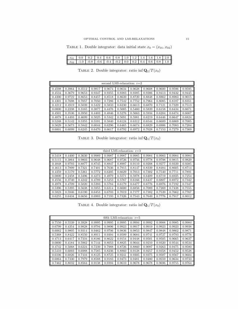
5.1.2. Numerical approximation. Table 1 displays the values of the initial statex0 ∈ X, and denoting inf Qr(x0) the optimal value of the LMI-relaxation (3.13) forthe minimum time OCP (5.1) with initial state x0, Tables 2, 3, and 4 display thenumerical values of the ratii inf Qr(x0)/T (x0) for r = 2, 3 and 5 respectively.
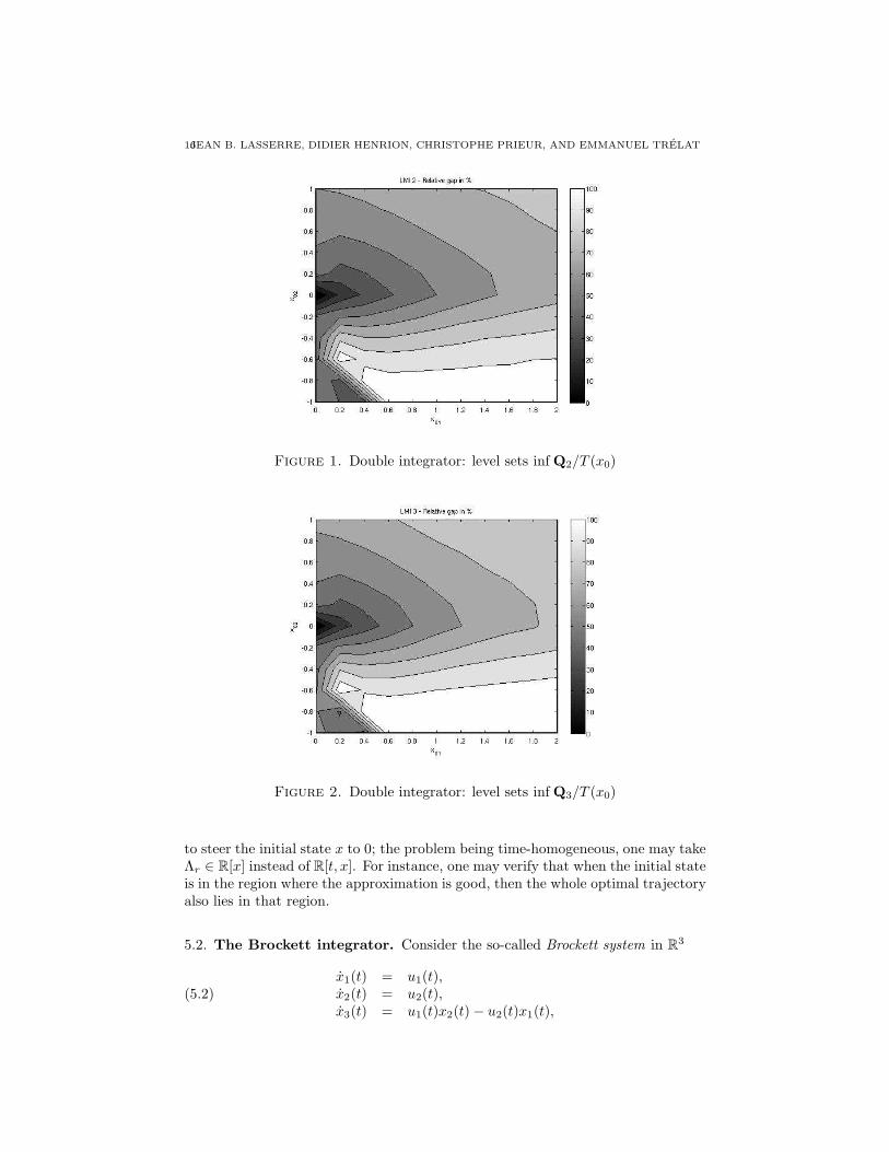
In Figures 1, 2, and 3 one displays the level sets of the ratii inf Qr/T (x0) forr = 2, 3 and 5 respectively. The closer to white the color, the closer to 1 the ratioinf Qr/T (x0).
Finally, for this double integrator example we have plotted in Figure 4 the levelsets of the function Λ5(x) − T (x) where T (x) is the known optimal minimum time
1 GloptiPoly 3 can be downloaded at www.laas.fr/∼henrion/software
OPTIMAL CONTROL AND LMI-RELAXATIONS 15
Table 1. Double integrator: data initial state x0 = (x01, x02)
x01 0.0 0.2 0.4 0.6 0.8 1.0 1.2 1.4 1.6 1.8 2.0
x02 -1.0 -0.8 -0.6 -0.4 -0.2 0.0 0.2 0.4 0.6 0.8 1.0
Table 2. Double integrator: ratio inf Q2/T (x0)
second LMI-relaxation: r=2
0.4598 0.3964 0.3512 0.9817 0.9674 0.9634 0.9628 0.9608 0.9600 0.9596 0.9595
0.4534 0.3679 0.9653 0.9347 0.9355 0.9383 0.9385 0.9386 0.9413 0.9432 0.9445
0.4390 0.9722 0.8653 0.8457 0.8518 0.8639 0.8720 0.8848 0.8862 0.8983 0.9015
0.4301 0.7698 0.7057 0.7050 0.7286 0.7542 0.7752 0.7964 0.8085 0.8187 0.8351
0.4212 0.4919 0.5039 0.5422 0.5833 0.6230 0.6613 0.6870 0.7121 0.7329 0.7513
0.0000 0.2238 0.3165 0.3877 0.4476 0.5005 0.5460 0.5839 0.6158 0.6434 0.6671
0.4501 0.3536 0.3950 0.4403 0.4846 0.5276 0.5663 0.5934 0.6204 0.6474 0.6667
0.4878 0.4493 0.4699 0.5025 0.5342 0.5691 0.5981 0.6219 0.6446 0.6647 0.6824
0.5248 0.5142 0.5355 0.5591 0.5840 0.6124 0.6312 0.6544 0.6689 0.6869 0.7005
0.5629 0.5673 0.5842 0.6044 0.6296 0.6465 0.6674 0.6829 0.6906 0.7083 0.7204
0.6001 0.6099 0.6245 0.6470 0.6617 0.6792 0.6972 0.7028 0.7153 0.7279 0.7369
Table 3. Double integrator: ratio inf Q3/T (x0)
third LMI-relaxation: r=3
0.5418 0.4400 0.3630 0.9989 0.9987 0.9987 0.9985 0.9984 0.9983 0.9984 0.9984
0.5115 0.3864 0.9803 0.9648 0.9687 0.9726 0.9756 0.9778 0.9798 0.9815 0.9829
0.4848 0.9793 0.8877 0.8745 0.8847 0.8997 0.9110 0.9208 0.9277 0.9339 0.9385
0.4613 0.7899 0.7321 0.7401 0.7636 0.7915 0.8147 0.8339 0.8484 0.8605 0.8714
0.4359 0.5179 0.5361 0.5772 0.6205 0.6629 0.7013 0.7302 0.7540 0.7711 0.7891
0.0000 0.2458 0.3496 0.4273 0.4979 0.5571 0.5978 0.6409 0.6719 0.6925 0.7254
0.4556 0.3740 0.4242 0.4789 0.5253 0.5767 0.6166 0.6437 0.6807 0.6972 0.7342
0.4978 0.4709 0.5020 0.5393 0.5784 0.6179 0.6477 0.6776 0.6976 0.7192 0.7347
0.5396 0.5395 0.5638 0.5955 0.6314 0.6600 0.6856 0.7089 0.7269 0.7438 0.7555
0.5823 0.5946 0.6190 0.6453 0.6703 0.7019 0.7177 0.7382 0.7539 0.7662 0.7767
0.6255 0.6434 0.6656 0.6903 0.7193 0.7326 0.7543 0.7649 0.7776 0.7917 0.8012
Table 4. Double integrator: ratio inf Q5/T (x0)
fifth LMI-relaxation: r=5
0.7550 0.5539 0.3928 0.9995 0.9995 0.9995 0.9994 0.9992 0.9988 0.9985 0.9984
0.6799 0.4354 0.9828 0.9794 0.9896 0.9923 0.9917 0.9919 0.9923 0.9923 0.9938
0.6062 0.9805 0.9314 0.9462 0.9706 0.9836 0.9853 0.9847 0.9848 0.9862 0.9871
0.5368 0.8422 0.8550 0.8911 0.9394 0.9599 0.9684 0.9741 0.9727 0.9793 0.9776
0.4713 0.6417 0.7334 0.8186 0.8622 0.9154 0.9448 0.9501 0.9505 0.9665 0.9637
0.0000 0.4184 0.5962 0.7144 0.8053 0.8825 0.9044 0.9210 0.9320 0.9544 0.9534
0.4742 0.5068 0.6224 0.7239 0.7988 0.8726 0.8860 0.9097 0.9263 0.9475 0.9580
0.5410 0.6003 0.6988 0.7585 0.8236 0.8860 0.9128 0.9257 0.9358 0.9452 0.9528
0.6106 0.6826 0.7416 0.8125 0.8725 0.9241 0.9305 0.9375 0.9507 0.9567 0.9604
0.6864 0.7330 0.7979 0.8588 0.9183 0.9473 0.9481 0.9480 0.9559 0.9634 0.9733
0.7462 0.8032 0.8564 0.9138 0.9394 0.9610 0.9678 0.9678 0.9696 0.9755 0.9764
16JEAN B. LASSERRE, DIDIER HENRION, CHRISTOPHE PRIEUR, AND EMMANUEL TRELAT
Figure 1. Double integrator: level sets inf Q2/T (x0)
Figure 2. Double integrator: level sets inf Q3/T (x0)
to steer the initial state x to 0; the problem being time-homogeneous, one may takeΛr ∈ R[x] instead of R[t, x]. For instance, one may verify that when the initial stateis in the region where the approximation is good, then the whole optimal trajectoryalso lies in that region.
5.2. The Brockett integrator. Consider the so-called Brockett system in R3
(5.2)x1(t) = u1(t),x2(t) = u2(t),x3(t) = u1(t)x2(t) − u2(t)x1(t),
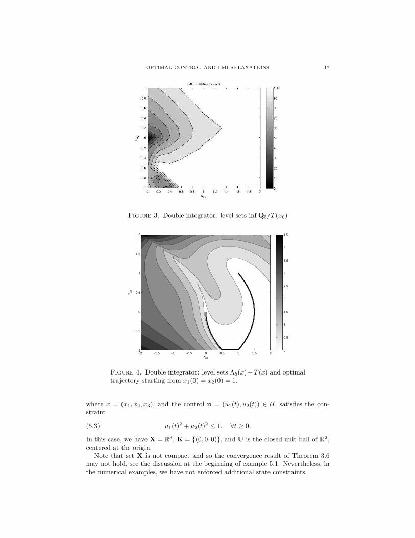
OPTIMAL CONTROL AND LMI-RELAXATIONS 17
Figure 3. Double integrator: level sets inf Q5/T (x0)
x01
x 02
−2 −1.5 −1 −0.5 0 0.5 1 1.5 2−1
−0.5
0
0.5
1
1.5
2
0
0.5
1
1.5
2
2.5
3
3.5
4
4.5
Figure 4. Double integrator: level sets Λ5(x)−T (x) and optimaltrajectory starting from x1(0) = x2(0) = 1.
where x = (x1, x2, x3), and the control u = (u1(t), u2(t)) ∈ U , satisfies the con-straint
(5.3) u1(t)2 + u2(t)
2 ≤ 1, ∀t ≥ 0.
In this case, we have X = R3, K = (0, 0, 0), and U is the closed unit ball of R
2,centered at the origin.
Note that set X is not compact and so the convergence result of Theorem 3.6may not hold, see the discussion at the beginning of example 5.1. Nevertheless, inthe numerical examples, we have not enforced additional state constraints.

18JEAN B. LASSERRE, DIDIER HENRION, CHRISTOPHE PRIEUR, AND EMMANUEL TRELAT
5.2.1. Exact computation. Let T (x) be the minimum time needed to steer an initialcondition x ∈ R
3 to the origin. We recall the following result of [2] (in fact givenfor equivalent (reachability) OCP of steering the origin to a given point x).
Proposition 5.2. Consider the minimum time OCP for the system (5.2) withcontrol constraint (5.3). The minimum time T (x) needed to steer the origin to apoint x = (x1, x2, x3) ∈ R
3 is given by
(5.4) T (x1, x2, x3) =θ√
x21 + x2
2 + 2|x3|√
θ + sin2 θ − sin θ cos θ,
where θ = θ(x1, x2, x3) is the unique solution in [0, π) of
(5.5)θ − sin θ cos θ
sin2 θ(x2
1 + x22) = 2|x3|.
Moreover, the function T is continuous on R3, and is analytic outside the line
x1 = x2 = 0.
Remark 5.3. Along the line x1 = x2 = 0, one has
T (0, 0, x3) =√
2π|x3|.
The singular set of the function T , i.e. the set where T is not C1, is the line x1 =x2 = 0 in R
3. More precisely, the gradients ∂T/∂xi, i = 1, 2, are discontinuous atevery point (0, 0, x3), x3 6= 0. For the interested reader, the level sets (x1, x2, x3) ∈R
3 | T (x1, x2, x3) = r, with r > 0, are displayed, e.g., in Prieur and Trelat [36].
5.2.2. Numerical approximation. Recall that the convergence result of Theorem3.6 is guaranteed for X compact only. However, in the present case X = R
3 is notcompact. One possibility is to take for X a large ball of R
3 centered at the originbecause for initial states x0 with norm ‖x0‖ relatively small, the optimal trajectoryremains in X. However, in the numerical experiments presented below, we havechosen to maintain X = R
3, that is, the LMI-relaxation Qr does not include anylocalizing constraint Mr−r(vj)(vj z(x)) 0 on the moment sequence z(x).
Recall that inf Qr ↑ minP as r increases, i.e., the more moments we consider,the closer to the exact value we get.
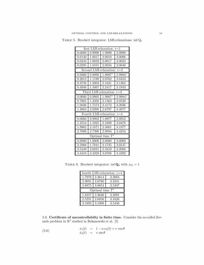
In Table 5 we have displayed the optimal values inf Qr for 16 different values ofthe initial state x(0) = x0, in fact, all 16 combinations of x01 = 0, x02 = 0, 1, 2, 3,and x03 = 0, 1, 2, 3. So, the entry (2, 3) of Table 5 for the second LMI-relaxationis inf Q2 for the initial condition x0 = (0, 1, 2). At some (few) places in the table,the ∗ indicates that the SDP solver encountered some numerical problems, whichexplains why one finds a lower bound inf Qr−1 slightly higher than inf Qr, whenpractically equal to the exact value T ∗.
Notice that the upper triangular part (i.e., when both first coordinates x02, x03
of the initial condition are away from zero) displays very good approximations withlow order moments. In addition, the further the coordinates from zero, the best.
For another set of initial conditions x01 = 1 and x0i = 1, 2, 3 Table 6 displaysthe results obtained at the LMI-relaxation Q4.
The regularity property of the minimal-time function seems to be an importanttopic of further investigation.
OPTIMAL CONTROL AND LMI-RELAXATIONS 19
Table 5. Brockett integrator: LMI-relaxations: inf Qr
first LMI-relaxation: r=10.0000 0.9999 1.9999 2.99990.0140 1.0017 2.0010 3.00060.0243 1.0032 2.0017 3.00240.0295 1.0101 2.0034 3.0040
Second LMI-relaxation: r=2
0.0000 0.9998 1.9997∗ 2.9994∗
0.2012 1.1199 2.0762 3.04530.3738 1.2003 2.1631 3.13040.4946 1.3467 2.2417 3.1943
Third LMI-relaxation: r=3
0.0000 0.9995 1.9987∗ 2.9984∗
0.7665 1.3350 2.1563 3.05301.0826 1.7574 2.4172 3.20361.3804 2.0398 2.6797 3.4077
Fourth LMI-relaxation: r=4
0.0000 0.9992 1.9977 2.99521.2554 1.5925 2.1699 3.04781.9962 2.1871 2.5601 3.19772.7006 2.7390 2.9894 3.4254
Optimal time T ∗
0.0000 1.0000 2.0000 3.00002.5066 1.7841 2.1735 3.05473.5449 2.6831 2.5819 3.20884.3416 3.4328 3.0708 3.4392
Table 6. Brockett integrator: inf Q4 with x01 = 1
fourth LMI-relaxation: r=41.7979 2.3614 3.20042.3691 2.6780 3.33412.8875 3.0654 3.5337
Optimal time T ∗
1.8257 2.3636 3.20912.5231 2.6856 3.34263.1895 3.1008 3.5456
5.3. Certificate of uncontrollabilty in finite time. Consider the so-called Zer-melo problem in R
2 studied in Bokanowski et al. [5]
(5.6)x1(t) = 1 − a x2(t) + v cos θx2(t) = v sin θ

20JEAN B. LASSERRE, DIDIER HENRION, CHRISTOPHE PRIEUR, AND EMMANUEL TRELAT
Figure 5. Zermelo problem: uncontrollable states with Q1
with a = 0.1. The state x is constrained to remain in the set X := [−6, 2]×[−2, 2] ⊂R
2, and we also have the control constraints 0 ≤ v ≤ 0.44, as well as θ ∈ [0, 2π].The target K to reach from an initial state x0 is the ball B(0, ρ) with ρ := 0.44.
With the change of variable u1 = v cos θ, u2 = v sin θ, and U := u : u21 + u2
2 ≤ρ2, this problem is formulated as a minimum time OCP with associated hierarchyof LMI-relaxations (Qr) defined in (3.13). Therefore, if an LMI-relaxation Qr atsome stage r of the hierarchy is infeasible then the OCP itself is infeasible, i.e., theinitial state x0 cannot be steered to the target K while the trajectory remains inX.
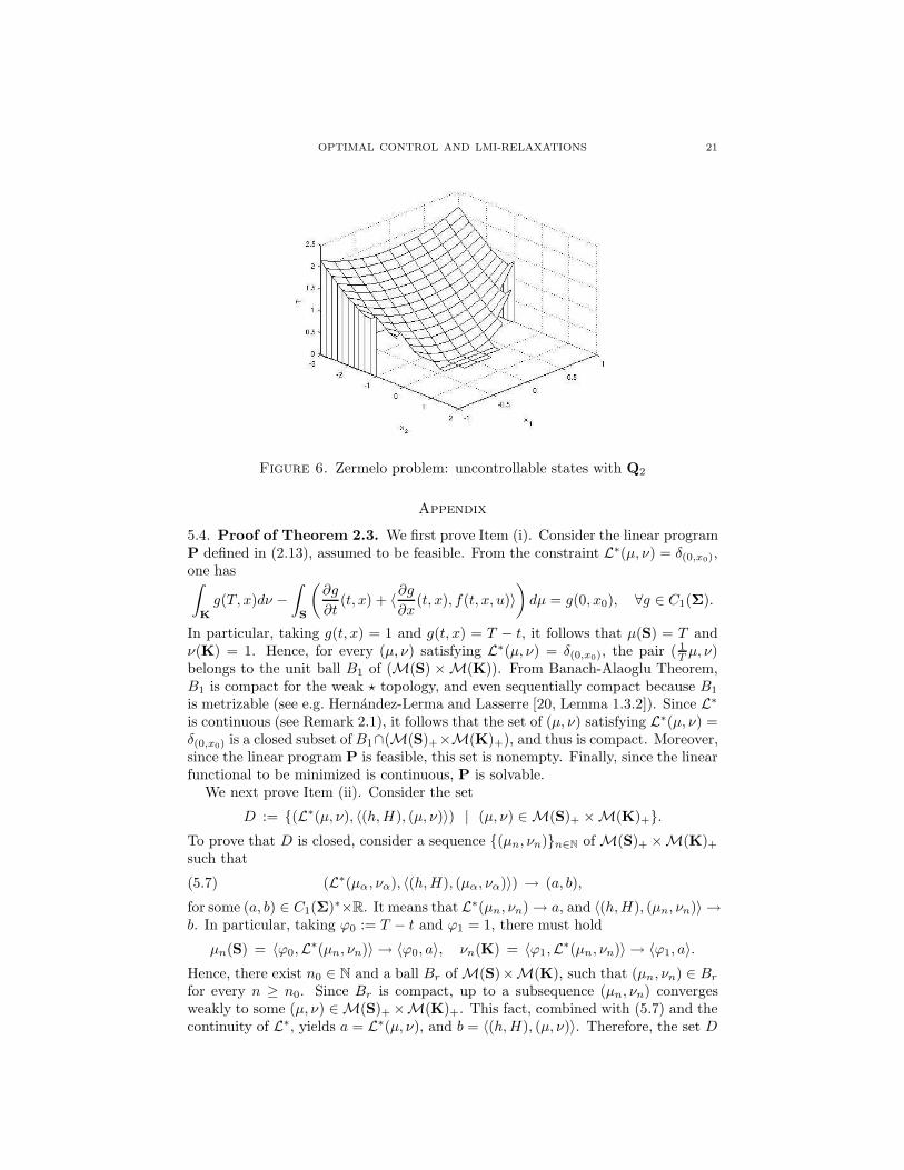
Figures 5 and 6 display the uncontrollable initial states x0 ∈ X found withthe infeasibility of the LMI-relaxations Q1 and Q2 respectively. With Q1, i.e.by using only second moments, we already have a very good approximation ofthe controllable set displayed in [5], and Q2 brings only a small additional set ofuncontrollable states.
OPTIMAL CONTROL AND LMI-RELAXATIONS 21
Figure 6. Zermelo problem: uncontrollable states with Q2
Appendix
5.4. Proof of Theorem 2.3. We first prove Item (i). Consider the linear programP defined in (2.13), assumed to be feasible. From the constraint L∗(µ, ν) = δ(0,x0),one has∫
K
g(T, x)dν −
∫
S
(
∂g
∂t(t, x) + 〈
∂g
∂x(t, x), f(t, x, u)〉
)
dµ = g(0, x0), ∀g ∈ C1(Σ).
In particular, taking g(t, x) = 1 and g(t, x) = T − t, it follows that µ(S) = T andν(K) = 1. Hence, for every (µ, ν) satisfying L∗(µ, ν) = δ(0,x0), the pair ( 1
T µ, ν)belongs to the unit ball B1 of (M(S) ×M(K)). From Banach-Alaoglu Theorem,B1 is compact for the weak ⋆ topology, and even sequentially compact because B1
is metrizable (see e.g. Hernandez-Lerma and Lasserre [20, Lemma 1.3.2]). Since L∗
is continuous (see Remark 2.1), it follows that the set of (µ, ν) satisfying L∗(µ, ν) =δ(0,x0) is a closed subset of B1∩(M(S)+×M(K)+), and thus is compact. Moreover,since the linear program P is feasible, this set is nonempty. Finally, since the linearfunctional to be minimized is continuous, P is solvable.
We next prove Item (ii). Consider the set
D := (L∗(µ, ν), 〈(h, H), (µ, ν)〉) | (µ, ν) ∈ M(S)+ ×M(K)+.
To prove that D is closed, consider a sequence (µn, νn)n∈N of M(S)+ ×M(K)+such that
(5.7) (L∗(µα, να), 〈(h, H), (µα, να)〉) → (a, b),
for some (a, b) ∈ C1(Σ)∗×R. It means that L∗(µn, νn) → a, and 〈(h, H), (µn, νn)〉 →b. In particular, taking ϕ0 := T − t and ϕ1 = 1, there must hold
µn(S) = 〈ϕ0,L∗(µn, νn)〉 → 〈ϕ0, a〉, νn(K) = 〈ϕ1,L
∗(µn, νn)〉 → 〈ϕ1, a〉.
Hence, there exist n0 ∈ N and a ball Br of M(S)×M(K), such that (µn, νn) ∈ Br
for every n ≥ n0. Since Br is compact, up to a subsequence (µn, νn) convergesweakly to some (µ, ν) ∈ M(S)+ ×M(K)+. This fact, combined with (5.7) and thecontinuity of L∗, yields a = L∗(µ, ν), and b = 〈(h, H), (µ, ν)〉. Therefore, the set D

22JEAN B. LASSERRE, DIDIER HENRION, CHRISTOPHE PRIEUR, AND EMMANUEL TRELAT
is closed.
From Anderson and Nash [1, Theorems 3.10 and 3.22], it follows that there isno duality gap between P and P∗, and hence, with (i), supP∗ = minP.
Item (iii) follows from Vinter [44, Theorems 2.1 and 2.3], applied to the mappings
F (t, x) := f(t, x, U) , l(t, x, v) := infu∈U
h(t, x, u) | v = f(t, x, u) ,
for (t, x) ∈ R × Rn.
5.5. Proof of Theorem 3.6. First of all, observe that Qr has a feasible solution.Indeed, it suffices to consider the sequences y and z consisting of the moments (upto order 2r) of the occupations measures νu and µu associated with an admissiblecontrol u ∈ U of the OCP (2.1)-(2.5).
Next, observe that, for every couple (y, z) satisfying all constraints of Qr, theremust holds y0 = 1 and z0 = 1. Indeed, it suffices to choose g(t, x) = 1 andg(t, x) = 1 − t (or t) in the constraint
Ly(g1) − Lz(∂g/∂t + 〈∇xg, f〉) = g(0, x0).
We next prove that, for r sufficiently large, one has |z(x)α| ≤ 1, |z(u)β| ≤ 1,|z(t)k| ≤ 1, for every k, and |yα| ≤ 1. We only provide the details of the proof forz(x), the arguments being similar for z(u), z(t) and y.
Let Σ2 ⊂ R[x] be the space of sums of squares (s.o.s.) polynomials, and letQ ⊂ R[x] be the quadratic modulus generated by the polynomials vj ∈ R[x] thatdefine X, i.e.,
Q := σ ∈ R[x] | σ = σ0 +∑
j∈J
σj vj with σj ∈ Σ2, ∀ j ∈ 0 ∪ J.
In addition, let Q(t) ⊂ Q be the set of elements σ of Q which have a representationσ0+
∑
j∈J σj vj for some s.o.s. family σj ⊂ Σ2 with deg σ0 ≤ 2t and deg σjvj ≤ 2tfor every j ∈ J .
Let r ∈ N be fixed. Since X ⊂ [−1, 1]n, there holds 1 ± xα > 0 on X, for everyα ∈ N
n with |α| ≤ 2r. Therefore, since X satisfies Putinar’ condition (see Definition3.4), the polynomial x 7→ 1 ± xα belongs to Q (see Putinar [37]). Moreover, thereexists l(r) such that x 7→ 1 ± xα ∈ Q(l(r)) for every |α| ≤ 2r. Of course, x 7→1 ± xα ∈ Q(l) for every |α| ≤ 2r, whenever l ≥ l(r).
For every feasible solution z of Ql(r) one has
|z(x)α| = | Lz(xα) | ≤ z0 = 1, |α| ≤ 2r.
This follows from z0 = 1, Ml(r)(z) 0 and Ml(r)−r(vj)(vj z(x)) 0, which implies
z0 ± z(x)α = Lz(1 ± xα) = Lz(σ0) +
m∑
j=1
Lz(x)(σj vj) ≥ 0.
With similar arguments, one redefines l(r) so that, for every couple (y, z) satisfyingthe contraints of Ql(r), one has
0 ≤ zk(t) ≤ 1 and |z(x)α|, |z(u)β|, |yα| ≤ 1, ∀ k, |α|, |β| ≤ 2r.
From this, and with l(r) := 2l(r), we immediately deduce that |zγ | ≤ 1 whenever|γ| ≤ 2r. In particular, Ly(H) + Lz(h) ≥ −
∑
β |Hβ | −∑
γ |hγ |, which proves thatinf Ql(r) > −∞, and so inf Qr > −∞ for r sufficiently large.

OPTIMAL CONTROL AND LMI-RELAXATIONS 23
Let ρ := inf P = minP (by Theorem 2.3), let r ≥ l(r0), and let (zr, yr) be a nearlyoptimal solution of Qr with value
(5.8) inf Qr ≤ Lzr(h) + Lyr(H) ≤ inf Qr +1
r
(
≤ ρ +1
r
)
.
Complete the finite vectors yr and zr with zeros to make them infinite sequences.Since for arbitrary s ∈ N one has |yr
α|, |zrγ | ≤ 1 whenever |α|, |γ| ≤ 2s, provided r
is sufficiently large, by a standard diagonal argument, there exists a subsequencerk and two infinite sequences y and z, with |yα| ≤ 1 and |zγ | ≤ 1, for all α, γ,and such that
(5.9) limk→∞
yrkα = yα ∀α ∈ N
n; limk→∞
zrkγ = zγ ∀γ ∈ N × N
n × Nm.
Next, let r be fixed arbitrarily. Observe that Mrk(yrk) 0 implies Mr(y
rk) 0whenever rk ≥ r, and similarly, Mr(z
rk) 0. Therefore, from (5.9) and Mr(yrk)
0, we deduce that Mr(y) 0, and similarly Mr(z) 0. Since this holds forarbitrary r, and |yα|, |zγ | ≤ 1 for all α, γ, one infers from Proposition 3.2 that yand z are moment sequences of two measures ν and µ with support contained in[−1, 1]n and [0, 1]× [−1, 1]n× [−1, 1]m respectively. In addition, from the equalitiesyrk
0 = 1 and zrk
0 = 1 for every k, it follows that ν and µ are probability measureson [−1, 1]n, and [0, 1]× [−1, 1]n × [−1, 1]m.
Next, let (t, α) ∈ N × Nn be fixed, arbitrarily. From
Lyrk (g1) − g(0, x0) − Lzrk (∂g/∂t + 〈∇xg, f〉) = 0, with g = (tpxα),
and the convergence (5.9), we obtain
Ly(g1) − g(0, x0) − Lz(∂g/∂t + 〈∇xg, f〉) = 0, with g = (tpxα),
that is, 〈Lg, (µ, ν)〉 = 〈g, δ(0,x0)〉. Since (t, α) ∈ N × Nn is arbitrary, we have
〈g,L∗(µ, ν)〉 = 〈L g, (µ, ν)〉 = 〈g, δ(0,x0)〉 ∀ g ∈ R[t, x],
which implies that L∗(µ, ν) = δ(0,x0).Let z(x), z(u) and z(t) denote the moment vectors of the marginals of µ with
respect to the variables x ∈ Rn, u ∈ R
m and t ∈ R, respectively, i.e.,
z(x)α =
∫
xα µ(d(t, x, u)) ∀α ∈ Nn, z(u)β =
∫
uβ µ(d(t, x, u)) ∀β ∈ Nm,
and z(t)k =∫
tk µ(d(t, x, u)) for every k ∈ N.With r fixed arbitrarily, and using again (5.9), we also have Mr(θjy) 0 for
every j ∈ JT , and
Mr(vj z(x)) 0 ∀ j ∈ J, Mr(wk z(u)) 0 ∀k ∈ W, Mr(t(1 − t) z(t)) 0.
Since X, K and U satisfy Putinar’s condition (see Definition 3.4), from Theorem3.5 (Putinar’s Positivstellensatz), y is the moment sequence of a probability measureν supported on K ⊂ [−1, 1]n. Similarly, z(x) is the moment sequence of a measureµx supported on X ⊂ [−1, 1]n, z(u) is the moment sequence of a measure µu
supported on U ⊂ [−1, 1]m, and z(t) is the moment sequence of a measure µt
supported on [0, 1]. Since measures on compact sets are moment determinate,it follows that µx, µu, and µt are the marginals of µ with respect to x, u and trespectively. Therefore, µ has its support contained in S, and from L∗(µ, ν) = δ(0,x0)
it follows that (µ, ν) satisfies all constraints of the problem P.

24JEAN B. LASSERRE, DIDIER HENRION, CHRISTOPHE PRIEUR, AND EMMANUEL TRELAT
Moreover, one has
limk→∞
inf Qrk= lim
k→∞Lzrk (h) + Lyrk (H) (by (5.8))
= Lz(h) + Ly(H) (by (5.9))
=
∫
h dµ +
∫
H dν ≤ ρ = minP.
Hence, (µ, ν) is an optimal solution of P, and minQr ↑ minP (the sequence ismonotone nondecreasing). Item (i) is proved.
Item (ii) follows from Theorem 2.3 (iii).
5.6. Proof of Theorem 4.1. It suffices to prove that vp → v as p → +∞. Forevery integer p, vp = minPp is attained for a couple of measures (µp, νp). As in theproof of Theorem 2.3, the sequence (µp, νp)p∈N is bounded in M(S)+ ×M(K)+,and hence, up to a subsequence, it converges to an element (µ, ν) of this space forthe weak ⋆ topology.
On the one hand, by definition, L∗p(µp, νp) = δ(0,x0) for every p. On the other,
L∗p tends strongly to L∗, and so L∗(µ, ν) = δ(0,x0). Moreover, since (hp, Hp) tends
strongly to (h, H) in C1(S) × C1(K), one has
vp = 〈(µp, νp), (hp, Hp)〉 −→ 〈(µ, ν), (h, H)〉,
and so v ≤ 〈(µ, ν), (h, H)〉. We next prove that v = 〈(µ, ν), (h, H)〉.Since (µp, νp) is an optimal solution of Pp,
〈(µp, νp), (hp, Hp)〉 ≤ 〈(µ, ν), (hp, Hp), ∀(µ, ν) | L∗p(µ, ν) = δ(0,x0).
Hence, passing to the limit,
〈(µ, ν), (h, H)〉 ≤ 〈(µ, ν), (h, H), ∀(µ, ν) | L∗(µ, ν) = δ(0,x0),
and so, (µ, ν) is an optimal solution of P, i.e., v = 〈(µ, ν), (h, H)〉.
Acknowledgments
The research of Didier Henrion was partly supported by Project No. 102/06/0652of the Grant Agency of the Czech Republic and Research Program No. MSM6840770038of the Ministry of Education of the Czech Republic.
References
[1] E.J. Anderson, P. Nash. Linear Programming in Infinite-Dimensional Spaces. John Wiley,Chichester, UK, 1987.
[2] R. Beals, B. Gaveau, P.C. Greiner. Hamilton-Jacobi theory and the heat kernel on Heisenberggroups. J. Math. Pures Appl. 79 (2000), 633–689.
[3] C. Berg. The multidimensional moment problem and semigroups. Proc. Symp. Appl. Math.
37 (1987), 110–124.[4] V. Borkar. Convex analytic methods in Markov decision processes. In: Hanbook of Markov
Decision Processes. E.A. Feinberg and A. Shwartz, Eds. Kluwer Academic Publishers, 2002,377–408.
[5] O. Bokanowski, S. Martin, R. Munos, H. Zidani. An anti-diffusive scheme for viability prob-lems. Submitted.
[6] R.W. Brockett. Asymptotic stability and feedback stabilization. In: Differential geometric
control theory. R.W. Brockett, R.S. Millman and H.J. Sussmann, Eds. Birkhauser, Boston,1983, pp. 181–191.
[7] I. Capuzzo-Dolcetta, P.L. Lions. Hamilton-Jacobi equations with state constraints. Trans.
Amer. Math. Soc. 318 (1990), 643–683.

OPTIMAL CONTROL AND LMI-RELAXATIONS 25
[8] Cho, Moon Jung, R.H. Stockbridge. Linear programming formulation for optimal stoppingproblems. SIAM J. Control Optim. 40 (2002), 1965–1982.
[9] C. Coatmelec. Approximation et interpolation des fonctions differentiables de plusieurs vari-ables. Annales Scientifiques de l’Ecole Normale Superieure, 3eme serie, 83, 4 (1966), 271–341.
[10] D.A. Dawson. Qualitative behavior of geostochastic systems. Stoch. Proc. Appl. 10 (1980),1–31.
[11] W.H. Fleming, D. Vermes. Convex duality approach to the optimal control of diffusions.SIAM J. Control Optim. 27 (1989), 1136–1155.
[12] R. Fletcher. Practical methods of optimization. Vol. 1. Unconstrained optimization. JohnWiley & Sons, Ltd., Chichester, 1980.
[13] P.E. Gill, W. Murray, M.H. Wright. Practical optimization. Academic Press, Inc., London-New York, 1981.
[14] R.F. Hartl, S.P. Sethi, R.G. Vickson. A survey of the maximum principles for optimal controlproblems with state constraints. SIAM Rev. 37 (1995), 181–218.
[15] K. Helmes, R.H. Stockbridge. Numerical comparison of controls and verification of optimalityfor stochastic control problems. J. Optim. Theory Appl. 106 (2000), 107–127
[16] K. Helmes, S. Rohl, R.H. Stockbridge. Computing moments of the exit time distribution forMarkov processes by linear programming. Oper. Res. 49 (2001), 516–530.
[17] D. Henrion, J.B. Lasserre. Solving nonconvex optimization problems. IEEE Control Systems
Magazine 24, 2004, pp. 72–83.[18] O. Hernandez-Lerma, J.B. Lasserre. Discrete-Time Markov Control Processes: Basic Opti-
mality Criteria. Springer Verlag, New York, 1996.[19] O. Hernandez-Lerma, J.B. Lasserre. Further Topics in Discrete-Time Markov Control Pro-
cesses. Springer Verlag, New York, 1999.[20] O. Hernandez-Lerma, J.B. Lasserre. Markov Chains and Invariant Probabilities. Birkhauser
Verlag, Basel, 2003.[21] O. Hernandez-Lerma, J.B. Lasserre. Approximation schemes for infinite linear programs,
SIAM J. Optim. 8, 1998, pp. 973–988.[22] O. Hernandez-Lerma, J.B. Lasserre. The linear programming approach, In: Hanbook of
Markov Decision Processes. E.A. Feinberg and A. Shwartz, Eds. Kluwer Academic Pub-lishers, 2002, pp. 377–408.
[23] D. Hernandez-Hernandez, O. Hernandez-Lerma, M. Taksar. The linear programming ap-proach to deterministic optimal control problems. Appl. Math. 24, 1996, pp. 17–33.
[24] M.W. Hirsch. Differential topology. Graduate Texts in Mathematics 33, Springer-Verlag,1976.
[25] D. Jacobson, M. Lele, J. L. Speyer. New necessary conditions of optimality for control prob-lems with state-variable inequality constraints. J. Math. Analysis Appl. 35 (1971) 255–284.
[26] J.L. Krivine. Anneaux preordonnes. J. Anal. Math. 12 (1964), 307–326.[27] T.G. Kurtz, R.H. Stockbridge. Existence of Markov controls and characterization of optimal
Markov controls. SIAM J. Control Optim. 36 (1998), 609–653.[28] J.B. Lasserre. Global optimization with polynomials and the problem of moments. SIAM J.
Optim. 11, 2001, pp. 796–817.[29] J.B. Lasserre, T. Prieto-Rumeau. SDP vs. LP relaxations for the moment approach in some
performance evaluation problems. Stoch. Models 20 (2004), 439–456.[30] J.B. Lasserre, T. Prieto-Rumeau, M. Zervos. Pricing a class of exotic options via moments
and SDP relaxations. Math. Finance 16 (2006), 469–494.[31] J.B. Lasserre, C. Prieur, D. Henrion. Nonlinear optimal control: Numerical approximations
via moments and LMI relaxations. Proc. 44th IEEE Conference on Decision and Control,Sevilla, Spain, December 2005, pp. 1648–1653.
[32] H. Maurer. On optimal control problems with bounded state variables and control appearinglinearly. SIAM J. Cont. Optim. 15 3 (1977) 345–362.
[33] J. Nash. The imbedding problem for Riemannian manifolds. Ann. Math. 63 (1956), 20–63.[34] H.J. Pesch. A practical guide to the solution of real-life optimal control problems. Control
Cybernet. 23, 1-2 (1994), 7–60.[35] L.S. Pontryagin, V.G. Boltyanskij, R.V. Gamkrelidze, E.F. Mishchenko. The Mathematical
Theory of Optimal Processes John Wiley & Sons, New York, 1962..[36] C. Prieur, E. Trelat. Robust optimal stabilization of the Brockett integrator via a hybrid
feedback. Math. Control Signals Systems 17, 3 (2005), 201–216.

26JEAN B. LASSERRE, DIDIER HENRION, CHRISTOPHE PRIEUR, AND EMMANUEL TRELAT
[37] M. Putinar. Positive polynomials on compact semi-algebraic sets. Ind. Univ. Math. J. 42,1993, pp. 969–984.
[38] K. Schmudgen. The K-moment problem for compact semi-algebraic sets. Math. Ann. 289
(1991), 203–206.[39] M.H. Soner. Optimal control with state-space constraints. SIAM J. Control Optim. 24 (1986),
552–561.[40] J. Stoer, R. Bulirsch. Introduction to Numerical Analysis. Third Edition, Springer-Verlag,
New York, 2002.[41] O. von Stryk, R. Bulirsch. Direct and indirect methods for trajectory optimization. Ann.
Oper. Res. 37, 1992, pp. 357–373.[42] E. Trelat. Controle optimal: theorie et applications. Vuibert, Paris, 2005. (in french)[43] F.-H. Vasilescu. Spectral measures and moment problems. Spectral Theory and Its Applica-
tions, Theta 2003, 173–215.[44] R. Vinter. Convex duality and nonlinear optimal control. SIAM J. Control Optim. 31, 2
(1993), 518–538.
LAAS-CNRS and Institute of Mathematics, University of Toulouse, France.
E-mail address: [email protected]
LAAS-CNRS, University of Toulouse, France and Czech Technical University in
Prague, Czech Republic.
E-mail address: [email protected]
LAAS-CNRS, University of Toulouse, France.
E-mail address: [email protected]
University of Orleans, France
E-mail address: [email protected]