Payment Contracts and Trade Financein Export Relationships

Christian Fischer∗

First draft: September 2016This version: July 2017

Preliminary version. Comments welcome.

Abstract. I examine the use of payment contracts in export partnerships whenthe importer’s payment moral is uncertain and there is a time gap between theproduction and sale of traded goods. In the absence of bank finance I find thatby deciding upon the payment format the exporter is challenged with a trade-offbetween maximizing the profits from the current transaction and making use ofscreening opportunities that differ between format types. Such screening can helpto attain information about the reliability of importers which is crucial to developefficient and intensive export relationships. Trade credit insurance can catalyzeexport growth and transaction profitability but its positive impact is limited to theinitial phase of export relationships.

Keywords: relational contracts, firm-level exports, trade finance, trade dynamics,contract enforcement

JEL-class.: L14, F10, F23, F34

∗Department of Economics, University of Bayreuth, Germany. Email:christian.fischer@uni-bayreuth.de.

The author thanks Fabrice Defever, Peter Egger, Paul Heidhues, Hans-Theo Normann,Jens Suedekum and seminar audiences in Dusseldorf and Gottingen for helpful comments andsuggestions. All errors are my responsibility.

1

1 Introduction

Shipping goods internationally is risky and takes time. Incomplete cross-border con-

tract enforcement exposes trading partners to an omnipresent risk of expropriation

(Thomas and Worrall 1994). At the same time, shipping and finally selling goods

abroad is time-consuming which challenges firms with a decision of how to finance

the working capital necessary for their export transactions. Taken together, these

aspects point at the importance of selecting an appropriate payment contract such

that risks and costs of exporting goods are managed optimally.1

Which trade-offs do trade partners face in their decision on the optimal payment

contract? Existing studies show that the (relative) costs of capital of exporter

and importer as well as the (relative) quality of contracting institutions in their

respective countries are crucial. When bank finance is considered the efficiency of

the relevant banking market also matters (see Schmidt-Eisenlohr 2013). Most of the

available literature frames firms’ payment contract choice in a static context, i.e. as a

situation where exporters and importers transact only once. However, a substantial

share of businesses worldwide interact with their export partners on a repeated basis

suggesting that the mechanics of payment contract selection in the dynamic context

of business relationships deserve more study.2 It is well-known from a literature on

incomplete relational contracts that repeated interaction can allow for self-enforcing

agreements between firms that can substitute for well-functioning legal institutions

(see e.g. Baker et al. 2002). As a consequence, existing static models on payment

contract choice may fundamentally mispredict the effective costs of financing trade

and therefore also the role of external bank or insurer finance that can help to

facilitate export activities.

In this paper I develop a repeated-game model of payment contract choice that

provides highly tractable predictions on the optimal sequence of payment contracts

in export relationships. At the same time it is general enough to cover any quality

of contracting institutions and applies to a wide range of refinancing costs and

demand characteristics that firms may face. The model shows that, when choosing

the payment contract type, the exporter faces a trade-off between maximizing the

payoffs from the current transaction and making use of the screening opportunities

1To finance the time gap between production and sale of traded goods the following categories ofpayment contracts exist: open account (exporter finance), cash in advance (importer finance) anddifferent types of bank-intermediated finance. For a comprehensive overview of payment methodsin international trade, see ITA (2007).

2There exists plenty of evidence that international business transactions frequently involve long-term collaboration. See e.g. Egan and Mody (1992), Rauch and Watson (2003), Besedes (2008)and Defever et al. (2016).

2

that differ inherently between format types. Such screening can help to attain

information about the reliability of importers which is crucial to develop efficient

and intensive export relationships.

Section 2 introduces the model. It considers an exporter (he) who sells a product

through an importer (she) abroad. The importer’s type is her private information

and acts as a measure of her costs of capital. In every period, the exporter proposes

a contract to his importer specifying an export quantity and a payment contract for

the current period. This contract can only be enforced with a certain probability that

depends on the quality of the contracting institutions of the participants’ countries.

The question of how to finance trade is relevant in the model because goods shipped

abroad can only be sold in the destination market in the subsequent period.

Section 3 then contrasts cash in advance and open account as diametrically op-

posed payment contract forms. I derive equilibria that study each of these payment

types in isolation and that highlight the fundamental differences between the con-

tracts. Most importantly, I show that while under cash in advance exporters can

offer a contract to importers that perfectly picks out reliable types, any open account

contract necessarily involves pooling of importers.

With this finding at hand, in section 4 the exporter can freely choose between

these two payment contracts leading to the trade-off between information acquisi-

tion and payoff maximization sketched above. As a corollary, the result allows to

give sharp predictions on the optimal sequence of payment contracts within an ex-

port relationship. Most importantly, this sequence depends on the distribution of

importer types and the quality of contracting institutions, among other factors.

Sections 5 introduces bank finance into the model and shows how the availability

of a trade credit insurance affects and augments the selection of payment contracts

in the dynamic context. Such an insurance can help to speed up export growth as

it can substitute for weak legal institutions. However, the benefits of such payment

guarantees are only temporary because in later periods an importer’s reputation for

reliability may make costly insurance redundant. Section 6 concludes.

This paper is relates to several lines of literature. A first strand studies pay-

ment contract selection and trade finance in international trade. Schmidt-Eisenlohr

(2013) was first to study the optimal choice between payment contracts in a strategic

environment, however his analysis is constrained to a static setting. Antras and Fo-

ley (2015) characterize the exporter’s payment contract choice with a similar setup.

Their analysis is motivated by stylized, empirical facts emerging from one specific

export industry in the United States. They also offer a dynamic version of the model

that gives predictions on how firms decide between cash in advance and open ac-

3

count payment contracts in the course of their export relationships. However, their

analysis cannot account for the fact that the two types of payment contracts allow

for very different learning possibilities about the importer’s reliability. Furthermore,

while their paper does not consider the role of bank finance in the dynamic context,

my model incorporates this possibility in the exporter’s choice set.

The role of banks and insurance firms in international trade finance has been the

subject of several studies. For the case of export credit insurances that I consider

in my model, most of the existing work has an empirical focus. Van der Veer (2015)

uses panel data from private trade credit insurers from 1992 to 2006 to show a pos-

itive effect of the existence of such insurances on exports. Auboin and Engemann

(2014) use data on the subsequent period of the financial crisis to demonstrate that

this positive effect remained stable over this time frame, i.e. it did not vary be-

tween crisis and non-crisis periods. Felbermayr and Yalcin (2013) study the effect

of export credit guarantees on exports in Germany and find qualitatively compara-

ble effects. These consistent findings are very much in line with Proposition 5 of

this paper where I show that the exporter can benefit from insuring transactions

to certain export destinations. Additionally, the result predicts that this positive

effect might be particularly driven by early transactions within export relationships.

Beyond export credit insurances, there exist several other types of bank-mediated

payment contracts. It is frequently documented, that letters of credit and documen-

tary collections are of particular importance and Schmidt-Eisenlohr and Niepmann

(2016) provide an insightful empirical study on the usage of these contract forms.

Olsen (2015) studies in a general equilibrium framework how banks’ reputation for

payment can be a valuable substitute for the trading partners’ own reputations and

weak legal institutions.3

Furthermore, the paper is related to a literature on learning and export dynam-

ics in trade relationships. Araujo et al. (2016) study how contract enforcement and

export experience shape firm export dynamics when information about importers

is incomplete. The learning mechanics on the importer type under the open ac-

count contract in my model are inspired by their setup, however the authors do not

use it to study questions related to trade finance. It is due to this learning that

exporters increase export volumes over time, a pattern that the authors confirm

empirically using a panel of Belgian exporters. Aeberhardt et al. (2014) provide

comparable results for French exporters. Building on Araujo et al. (2016), Monarch

and Schmidt-Eisenlohr (2016) document that there exists substantial heterogeneity

3A survey of this literature in the broader context of corporate finance in international tradecan be found in Foley and Manova (2015).

4

in how export-relationships mature in different countries. This is consistent with my

model as it predicts that country- and/or industry-specific characteristics (through

the quality of legal institutions and the type distribution of importers) matter for

the selection of payment contracts.

Finally, my model is related to a literature on self-enforcing relational contracts

with incomplete information and adverse selection that were first studied by Levin

(2003). More specifically, it adds to a growing literature on non-stationary relational

contracts with adverse selection, in which contractual terms vary with the length

of relationships. While in my paper learning about the importer induces switching

between different payment contracts, previous work has studied non-stationarities

in other contexts. Chassang (2010) studies how agents with conflicting interests

can develop successful cooperation when details about cooperation are not common

knowledge. Halac (2012) studies optimal relational contracts when the value of a

principal-agent relationship is not commonly known and, also, how information rev-

elation affects the dynamics of the relationship. Yang (2013) studies firm-internal

wage dynamics when worker types are private information. Board and Meyer-ter

Vehn (2015) analyze labor markets in which firms motivate their workers through

relational contracts and study the effects of on-the-job search on employment con-

tracts. Moreover, Defever et al. (2016) study buyer-supplier relationships in which

learning about the quality of a supplier can cause switches in the contractual nature

of these relationships.

2 The Model

The model builds on Araujo et al. (2016) and extends their setting to study the

dynamic selection of payment contracts. It considers the problem of an exporter

from country Home that markets a product in a foreign market (Foreign). The

exporter cannot access foreign consumers directly and needs to contract with an

importer in order to make products available to consumers. In Foreign, there is

a continuum of agents with the ability to internally distribute goods produced by

the exporter. Each exporter is a monopolist and has constant marginal costs c

for the production of his output. The revenue from selling q units of the product

in Foreign generates revenue R, which we assume to be a strictly increasing and

concave function of q, i.e.

R = R(q), with R′(q) > 0, R′′(q) < 0, and R(0) = 0. (1)

5

Whether the concavity of the revenue function stems from technology, preferences

or market structure is not important for the analysis below. The revenue is realized

by the importer.

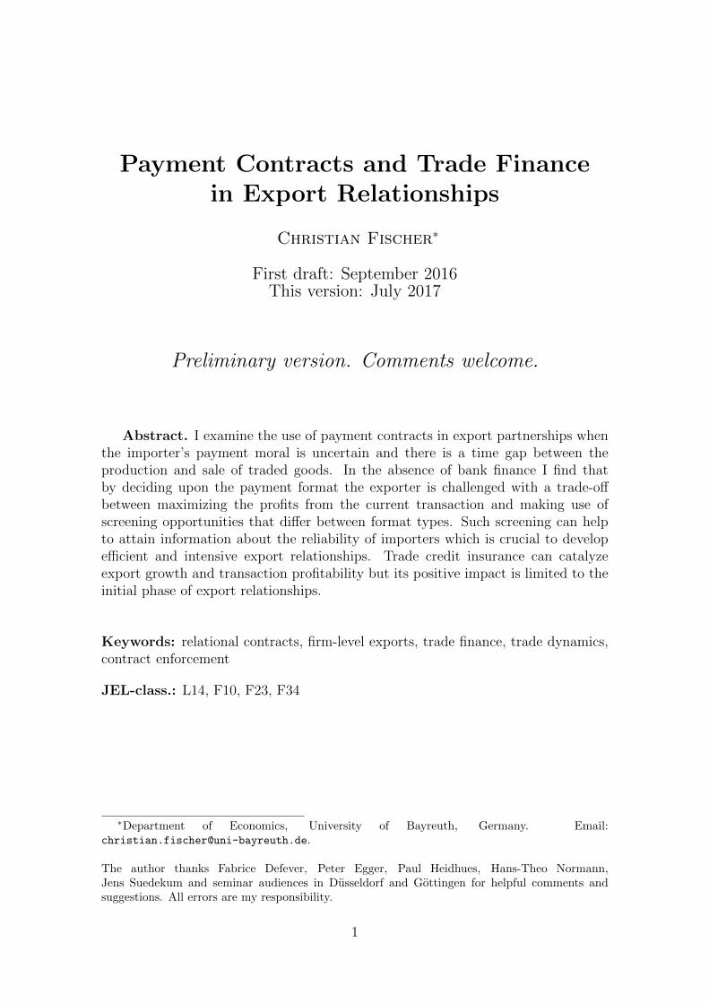
We model the export relationship as a repeated game, where in every period

t = 0, 1, 2, ... an export transaction is performed. The exporter can engage in only

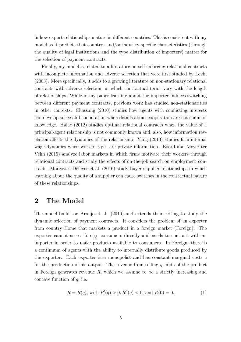
one partnership at the same time. Figure 1 gives an intuitive summary of the stage

game. In every period t, the exporter first decides whether to start a relationship

with a new importer or to keep his previous one. He then proposes a contract to his

importer specifying export volume, a payment from importer to exporter and the

point in time when this payment is made. Depending on the agreed payment timing,

the exporter will receive the transfer either before he ships out his goods (Cash in

Advance, Ft = CIA) or after the importer sells them in Foreign (Open Account,

Ft = OA). The timing of the transfer is directly payoff relevant because shipping

the goods from Home to Foreign takes time. We model this aspect by assuming that

the goods can be sold in Foreign only at the beginning of the subsequent period t+1.

Matching Contracting Shipment Sale

Payment

t t + 1

Ft = CIA Ft = OA

Figure 1: Payment contract determines the stage game timing

As the game shifts from one period to the next players discount their expected

payoffs, potentially at different rates. Such an asymmetry may be interpreted as

interest rates and thus costs of capital that differ between Home and Foreign, but

may also be the result of other institutional differences. Formally, we denote the

exporter’s discount factor as δE ∈ (0, 1). In order that payment contract selection is

non-trivial we assume two types of importers that the exporting firm may encounter.

Her type is the importer’s private information. A share θ of importers is myopic

with discount factor δM = 0, i.e. these importers only give positive value to payoffs

that are realized in the current period. The remaining 1 − θ importers are patient

with discount factor δI ∈ (0, 1). Absent additional information, the exporter holds

the prior belief θ0 = θ that a randomly chosen importer is myopic.

The quality of the contracting institutions in Home and Foreign come into the

model through an exogenous country-specific probability that a contract is enforced

when firms do not want to fulfill it voluntarily, a concept originating from Schmidt-

Eisenlohr (2013). More specifically, in every period of the game a spot contract Ct

6

specified below can be enforced in country Foreign (Home) with the i.i.d. probability

λ (λ∗). In the model, λ is the probability that the importer is forced make the agreed-

upon payment to the exporter for the period t transaction while λ∗ is the probability

that the exporter is being forced to produce and ship abroad the agreed-upon volume

of exports.

In the following a formal representation of the stage game that introduces further

notation and assumptions:

Stage game.

1. Revenue realization. The qt−1 units shipped in the previous period arrive

in Foreign. The importer generates revenue R(qt−1).

2. Payment (if Ft−1 = OA). The importer decides whether to transfer Tt−1 =

βR(qt−1), 0 < β < 1, to the exporter. He (costlessly) finds an opportunity to

only pay a transfer Tt−1 = γR(qt−1), 0 ≤ γ < β, with probability 1− λ. Upon

contract non-compliance the match is permanently dissolved.

3. Matching decision. Whenever unmatched, the exporter starts a new part-

nership. Otherwise, the exporter chooses whether to stick to the current im-

porter or to re-match with a new partner.

4. Contracting.

• The exporter proposes a one-period spot contract Ct = qt, Ft, Tt to the

importer. The contract specifies the units qt of the exporter’s product to

be sold by the importer, and a trade finance arrangement Ft for period t,

where Ft ∈ F = CIA,OA. The choice of Ft determines the timing of

the transfer payment Tt = βR(qt) from the importer to the exporter that

is a fraction of the revenue. We make the restriction to spot contracts to

reduce the screening possibilities in the model to a tractable minimum.

• The importer decides whether to accept or reject the contract. Upon

rejection, the match is permanently dissolved and a new match is formed

in the following period.

5. Payment (if Ft = CIA). The importer decides whether to transfer Tt to the

exporter. Upon non-payment the match is permanently dissolved.

6. Production and Shipment. The exporter decides whether to produce and

ship qt units of his goods to the importer as specified in the contract. He

(costlessly) finds an opportunity to deviate from the contracted terms with

7

probability 1 − λ∗. Upon non-shipment of the agreed quantity the match is

permanently dissolved.

3 The nature of payment contracts

Before discussing how a payment contract is selected in the presence of several

alternatives and how this choice varies over time, this section studies each of the

two alternatives in isolation. We explore for every payment format separately, how

information about the importer is revealed and how the export intensity changes

over time. The payment type selection in the dynamic context of the model is

discussed in the subsequent section.

In the following, we derive equilibria for both cases, CIA and OA, that are highly

comparable but highlight important differences resulting from the nature of the two

payment contracts.

3.1 Cash in advance

In this section we study the case where the exporter is restricted to cash in advance,

i.e. Ft = CIA for all t. Consider the following strategy profile that we will show to

be part of a sequential equilibrium of the repeated game.4

CIA strategy profile.

• Exporter strategy: The exporter forms a new partnership whenever un-

matched. He terminates an existing partnership if and only if the importer

defaults on the contract. The exporter proposes a contract Ct that maximizes

his current period expected payoffs.

• Importer strategy: A myopic importer will reject any CIA contract. A

patient importer never defaults from the proposed contract.

The importers’ participation constraints for period t are:

(δi − β)R(qt) ≥ 0, where i = M, I. (PCAi )

The constraints state, that tomorrow’s revenue R(qt) attained by the sale of today’s

exports qt must be larger than the the share β of revenue that the importer has to

transfer to the exporter before shipping. Because the goods arrive in Foreign only

4For adverse selection scenarios as we study them here, sequential equilibrium is the relevantnotion of equilibrium, see Mailath and Samuelson (2006), pp. 158–159.

8

in the following period revenue has to be discounted. Observe that because δM = 0,

(PCAM) cannot be fulfilled for any β ∈ (0, 1). Hence the myopic importer will never

accept any CIA contract. The exporter will therefore offer a separating contract to

the patient importer and set β to extract all rents from her.

With this in mind, suppose that we are in the initial period k = 0 of a newly

matched export relationship. At the contracting stage, the exporter will set the

export quantity q0 and a transfer payment T0 that maximizes his spot payoffs subject

to the participation constraint of the patient importer:

maxq0

(1− θ0)(βR(q0)− cq0) s.t. (δI − β)R(q0) ≥ 0.

The exporter chooses the exported quantity q0 such that it maximizes his share

of the revenue βR(q0) minus the costs of production, and subject to (PCAI ). The

payoff is weighted by the probability of facing a patient importer 1− θ0 since non-

participation of the myopic type leads to zero payoffs. The exporter sets βA = δI to

make the patient importer indifferent between accepting and rejecting the contract

and to receive the maximally feasible share of the revenue. This simplifies the

maximization problem to:

maxq0

(1− θ0)(δIR(q0)− cq0).

The producer’s optimal export quantity under cash in advance, QA, is determined

by the related first-order condition (FOC):

R′(q0) =c

δI.

Once an initial CIA export transaction is successful the exporter knows for sure

that he is matched with a patient type. We can write the belief that the importer

is myopic given k previous successful transactions under cash in advance as:

θAk =

θ0 if k = 0,

0 if k > 0.

Because the FOC for the initial transaction is already belief-independent it fol-

lows that QA is the same for every cash in advance transaction. The expected payoffs

in the initial period of a CIA relationship thus are:

πA0 ≡ πA(θA0 ) = (1− θ0)(δIR(QA)− cQA).

9

In any subsequent transaction the exporter expects to receive the following payoffs:

πA ≡ πA(θAk = 0) = δIR(QA)− cQA. (2)

Because the production and shipment decision is made after the transfer payment

under a CIA contract, we need to ensure that the exporter does not have an incentive

to deviate and not ship out his goods as agreed upon. The following Lemma gives

a simple condition that rules out any such deviation.

Lemma 1. For every θ0 ∈ ( cQA

πA, 1) there exists a unique δE = cQA

θ0πAsuch that the

exporter never deviates at the Production and Shipment stage if and only if δE ≥ δE.

Proof. See Appendix

Lemma 1 shows that if the mass of myopic types in the population of potential

importers is not too small, it is always optimal for sufficiently patient exporters

(those with δE ≥ δE) to ship the contracted goods to the importer who paid for them

beforehand. If however the mass of myopic types is too small breach of contract by

the exporter cannot be avoided because he finds it too likely to draw again a patient

type in the following period where, again, he could cash the transfer, refrain from

shipping and re-match.

The following Proposition summarizes our findings on the cash in advance equi-

librium.

Proposition 1. Suppose only cash in advance payments are possible. The ex-

porter starts a partnership whenever he finds a match, maintains the partnership as

long as he does not observe a default, and exports QA in each period k in which the

partnership is active. A myopic importer never participates under cash in advance.

A patient importer never defaults and never terminates a partnership. This strategy

profile together with the belief updating rule θAk is a sequential equilibrium.

There are several points noteworthy about the equilibrium. First, a cash in

advance contract is very demanding with respect to the financial capabilities of the

importer. This aspect is stressed in our model by the fact that impatient importers

are fully myopic which precludes them from accepting the contract. Therefore any

CIA contract in the present model is a separating contract that perfectly screens

out patient importers. As a consequence, learning about the importer’s type under

CIA is immediate. After the initial period of interaction, the exporter knows with

certainty the type of his current match.

10

Certainly, assuming full myopia of the impatient type is a strong assumption

and immediate separation of types the extreme consequence. However, the result

is very illustrative when contrasted with the screening mechanism available under

open account introduced in the following section.

3.2 Open account

We now study the case where the exporter is restricted to open account contracts,

i.e. Ft = OA for all t. Essentially, this version of our model is a stripped-down

variant of the setup by Araujo et al. (2016). Consider the following strategy profile

that we will show to be part of a sequential equilibrium of the repeated game.

OA strategy profile.

• Exporter strategy: The exporter forms a new partnership whenever un-

matched. He terminates an existing partnership if and only if the importer

defaults on the contract. The exporter proposes a contract Ct that maximizes

his current period expected payoffs.

• Importer strategy: Both, myopic and patient importer accept the OA con-

tract. While the patient importer never defaults, the myopic importer will

default whenever she finds the opportunity to do so.

With this strategy in mind we can write the participation constraints of the two

types as:

(1− β)R(qt) ≥ 0, (PCΩI )

(1− λβ)R(qt) ≥ 0, (PCΩM)

where (PCΩI ) is the participation constraint of the patient importer and (PCΩ

M) that

of the myopic importer, respectively. While it is possible to construct a separating

contract that picks up only patient importers under CIA, this is not possible for OA.

Myopic importers only make a transfer when exporters can enforce their contract

(which happens with probability λ). This makes their PC more lenient. Because

0 < β < 1, it follows that every feasible OA transaction involves pooling of importer

types. Besides, discounting does not affect the importer’s participation decision

since revenue realization and payment for a period t contract are both made in t+1.

Suppose for the moment that importers behave as prescribed by the strategy

profile and consider belief formation. In the initial period of a partnership, k = 0,

the exporter believes that he is matched with a myopic type with probability θ0 = θ.

11

According to the strategy profile patient agents never deviate and myopic types

always want to deviate but in every period this is only possible if contracts cannot

be enforced. This happens with probability 1− λ. Hence, if no deviation occurs in

the course of the first k transactions, the belief of facing a myopic type in period k

is updated by Bayes’ rule as follows:

θΩk =

θλk

1− θ(1− λk).

The probability of payment in the initial period can be written as Λ0 = 1−θ0 +λθ0.

More generally, the probability of payment in period k is Λk = 1−θ(1−λk+1)

1−θ(1−λk).

Observe that in order to make the patient importer behave as described by the

strategy profile, it is not enough to merely consider her participation constraint as

we did in the CIA case. Under open account, she must be granted a payoff such

that she does not seize the revenue realized by her instead of making the transfer

payment. We denote the maximal share of revenue that the importer is able to seize

by 1−γ, where 0 ≤ γ < β is the exogenous revenue share that the exporter can still

claim under any importer deviation.We can formulate the following Lemma:

Lemma 2. There exists a unique δI = β−γ1−γ such that the importer never deviates

at the Payment stage of any period of an export relationship if and only if δI ≥ δI .

Equivalently, a patient importer will never deviate from the contract if and only if

β ≤ δI + γ(1− δI) ≡ βΩ. (ICΩI )

Proof. See Appendix

The Lemma states, that as long as the share of revenue that has to be transfered

to the exporter is below the threshold level βΩ, the patient importer has no incen-

tive to deviate from the accepted contract. Obviously, payment is never incentive

compatible for a myopic importer who will refrain from transferring βΩ whenever

possible.

Let us now turn to the exporter’s maximization problem. In any period k of the

export relationship he chooses qk to maximize:

maxqk

δEΛkβR(qk)− cqk s.t. β ≤ βΩ.

While the exporter has to bear the costs of production cqk already today, he will

receive the expected transfer ΛkβR(qk) only in the following period which is therefore

12

discounted by δE. The exporter wants to extract the maximum possible transfer from

the importer and he will set β such that (ICΩI ) binds with equality, i.e. β = βΩ. The

unconstrained maximization problem of the exporter for transaction k of an export

relationship thus is:

maxqk

δEΛkβΩR(qk)− cqk

The FOC to this problem can be written as:

R′(qk) =c

δEΛkβΩ,

implying that the producer’s optimal export quantity under OA, QΩk , depends on

his belief θk and is increasing in k (since the probability of payment Λk is increasing

in k). We can write the expected exporter payoff from an open account transaction

in period k of the export relationship as:

πΩk ≡ πΩ(θΩ

k ) = δEΛkβΩR(QΩ

k )− cQΩk .

Observe that with the export relationship growing mature, the probability of pay-

ment Λk converges to one. The exported quantity therefore also converges to a limit

value that we denote by QΩ. We denote the payoffs that the exporter receives at

this limit as:

πΩ ≡ πΩ(θΩk = 0) = δEβ

ΩR(QΩ)− cQΩ. (3)

The following Proposition summarizes our findings on the open account equilibrium.

Proposition 2. Suppose only open account payments are possible. The exporter

starts a partnership whenever he finds a match, maintains the partnership as long

as he does not observe a default, and exports QΩk in the k-th period of any active

partnership. A myopic importer deviates from the contract whenever she has the

opportunity. A patient importer never defaults. Both types never terminate a part-

nership. This strategy profile together with the belief updating rule θΩk is a sequential

equilibrium.

3.3 Comparing the payment contract equilibria

There are several noteworthy differences between export relationships with CIA and

OA payment contracts. First, while learning about the importer’s type under CIA is

immediate (see updating rule θAk ) information acquisition under OA is only gradual

(see θΩk ). The reason is that while the exporter can design the CIA contract to only

13

attract patient importers, OA necessarily involves pooling which makes it necessary

for patient importers to build up a reputation for reliability.

Second, since under CIA there is no risk involved in any transaction for the ex-

porter (since payment is made before production) he will export the ex-post optimal

quantity QA starting with the very first transaction. In contrast, under OA the ex-

port decision is risky because payment takes place after production. Additionally,

since the exporter can only use pooling contracts the optimal export quantity QΩk is

adjusted by the importer’s reputation of being a patient type and therefore increases

gradually over time (up to QΩ, for k →∞).

The first two points together imply the following for the exporter’s expected

payoff. Given that he is matched to a patient type, under CIA the payoff will after

the initial period immediately jump from πA0 to the maximum πA. Under OA, it

will starting from πΩ0 increase gradually in the course of the relationship up to the

maximum πΩ.

4 Dynamic selection of payment contracts

In this section we relax the restriction to one specific payment contract and allow

the exporter to freely choose in every period k of the export relationship whether

to employ CIA or OA. At the Contracting stage of every period t the exporter

thus decides on an element Ft ∈ F = CIA,OA. Essentially, we explore how the

exporter decides between the CIA and OA equilibrium derived in Propositions 1

and 2 and how this choice varies over time, as beliefs about the matched importer

evolve.

For both payment formats the expected exporter stage game payoff is highest

with all uncertainty about the importer’s patience being resolved, i.e. when the

exporter is certain to be facing a patient type. This is the case when θAk = 0

and θΩk = 0, respectively. Comparison of the related payoffs in equations (2) and

(3) suggests that πΩ ≥ πA whenever βΩδE ≥ δI , and πΩ ≤ πA otherwise. In

the main text, we focus on the scenario where under complete information OA is

more profitable than CIA, i.e. the case where βΩδE > δI . We thus capture the

scenario where δE > δI , i.e. the exporter has relatively low costs of capital while

the importer faces relatively high costs of capital. From a modeling perspective,

this case is particularly interesting because while OA is not learning-optimal for the

exporter it gives him the largest long-run payoffs. In the Appendix, we also briefly

discuss the reverse situation.

14

4.1 Main result

The comparison of the two payment contracts in section 3.3 hints at the latent trade-

off in the design of the dynamically optimal series of spot contracts between acquiring

information about the importer and using the payment contract that promises the

largest spot payoff. In this section we study how the exporter should optimally

design the series of spot export contracts, i.e. how he should over time select between

the two possible payment contracts in the form of the two equilibria derived in

Propositions 1 and 2. To keep the analysis tractable, we assume that the exporter

has to decide for one specific payment contract and cannot propose a whole menu

of contracts to the importer.

In order to understand payment contract selection it is important to observe

that i) open account is maximizing the exporter’s payoff under full information, i.e.

πΩ > πA, ii) for each payment contract the exporter’s payoff is maximal under full

information, and iii) learning the importer’s type under CIA is immediate. The

three points together imply that if a CIA transaction is successfully conducted any

further transaction with this importer will be on OA and involve export quantity

QΩ and exporter payoffs πΩ.

With this in mind, let us assume that the importer’s type has not yet been

learned, i.e. OA has been played up to period k of the relationship. In choosing

the transaction’s payment contract the exporter has to decide whether he wants to

learn the true type of the importer today (through switching to CIA for the current

transaction) or whether to continue with the OA format, at least until the following

period k+1 in which he can reconsider. Formally, the exporter will conduct the kth

transaction through open account if and only if

πΩk + δEπ

A(θΩk+1) +

δ2E

1− δEπΩ ≥ πA(θΩ

k ) +δE

1− δEπΩ, (4)

where πA(θΩk ) and πA(θΩ

k+1) denote the exporter’s expected payoffs under CIA for

beliefs θΩk and θΩ

k+1, respectively, that are derived from the open account updating

rule. Using this expression we obtain the following Proposition.

Proposition 3. Suppose that δE >δIβΩ , i.e. OA is payoff-maximal with perfect

information about the importer’s type. Also suppose that θ0 ≥ cQA

δEπA ≡ θ0, i.e.

Lemma 1 holds. Consider the kth transaction in an export relationship. The exporter

will conduct this transaction through Open Account if and only if

πΩk − πA(θΩ

k ) ≥ δE[πΩ − πA(θΩ

k+1)]

(5)

15

and ask for Cash in Advance otherwise.

The inequality in (5) is obtained from rearranging (4) and provides a necessary

and sufficient condition whether any transaction of an export relationship is con-

ducted through either CIA or OA. Intuitively, it states that OA will be chosen for

the current transaction if today’s payoff gain from choosing OA instead of CIA is

larger than tomorrow’s payoff gain from OA when using the more screening-efficient

CIA contract today. Note, that expression (5) is always fulfilled when the importer’s

type has been revealed in the past, e.g. when a CIA has been conducted. I provide

a more extensive discussion of the result in the following subsection.

4.2 Discussion

The results up to now are formulated fairly generally and to make their discussion

illustrative we make an additional but unrestrictive assumption for the revenue

function. We let R(q) = q1−α

1−α , where the parameter α, with 0 < α < 1, determines

the concavity level of the revenue function. Note that this function captures all the

properties that we had assumed in (1) and is general enough to capture arbitrary

levels of concavity. This functional form allows us to obtain simple expressions for

many of the previously derived results. Importantly for the discussion of Proposition

3, πΩk = Λ

′ 1αk π

Ω and πΩ =(δEβ

Ω

δI

) 1απA. With Λ′k = 1 − θ′k(1 − λ) we denote the

probability of payment for some belief θ′k. The expressions allow us to rewrite (5)

as:

I(θ′k, λ, δI , δE, α, γ) ≡ Λ′1αk − δE +

(δI

δEβΩ

) 1α (δE − Λ′k)(1− θ′k)

Λ′k≥ 0, (6)

which determines whether the kth transaction of an export relationship is conducted

via OA (if I > 0) or via CIA (if I < 0). Observe that in I(·) the variables λ, δI , δE,

α and γ are all constants for a given export relationship. Within a relationship the

value of I(·) only changes with the belief θ′k of facing a myopic importer. This belief

can be characterized as:

θ′k =

θΩk if I > 0 for all previous transactions, or when k = 0,

0 if I < 0 in some previous transaction.(7)

Note also, that the expression for the minimal initial belief of facing a myopic type

from Lemma 1 that is necessary for equilibrium existence simplifies to θ0 = 1−αδEα

.

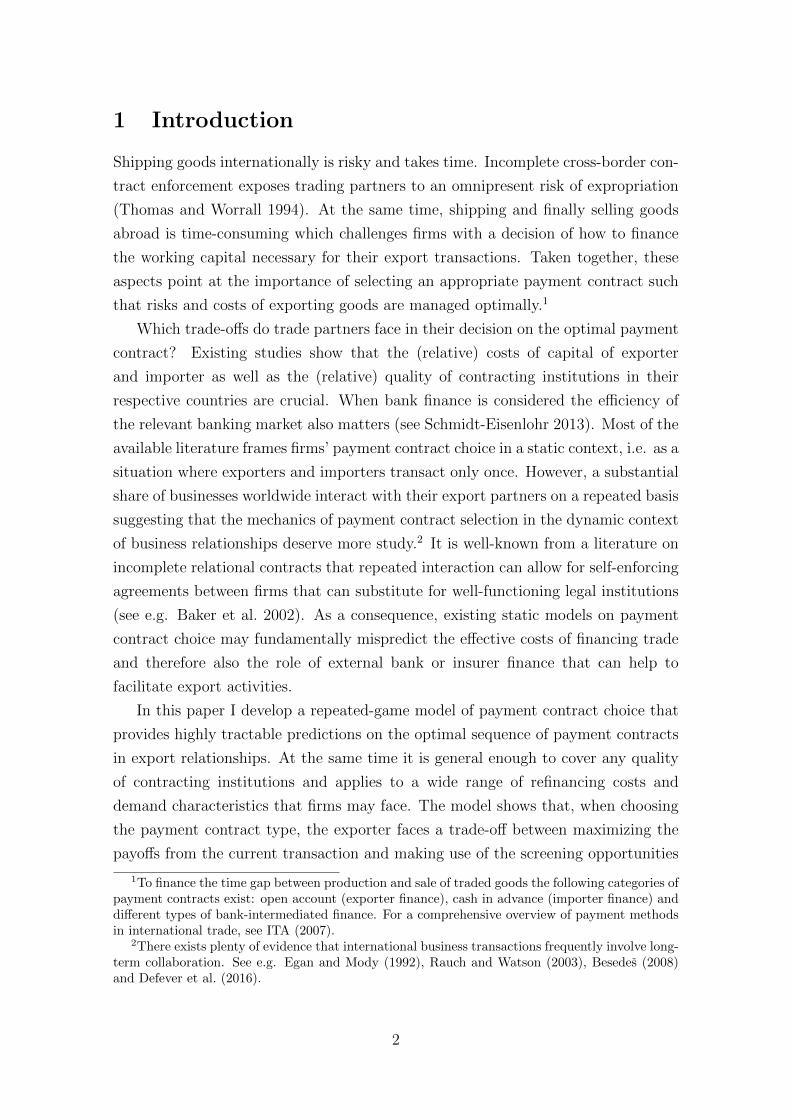
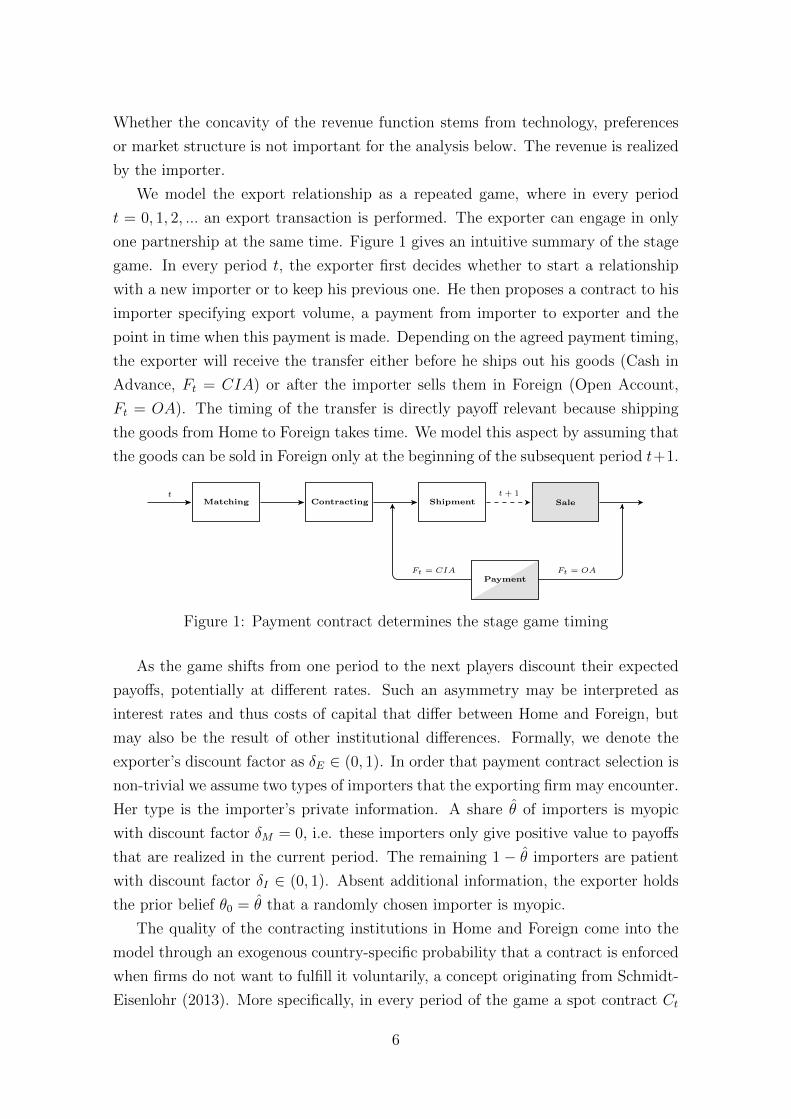
The predictions of Proposition 3 in the form of expressions (6) and (7) are best

explained by making use of their graphical representations in Figure 2. The sub-

figures (a) and (b) show for all possible combinations of initial belief θ0 and contract

16

enforceability in Foreign λ which payment contract will be used in the initial and

(conditional on continuation) in the subsequent period of the export relationship,

respectively.

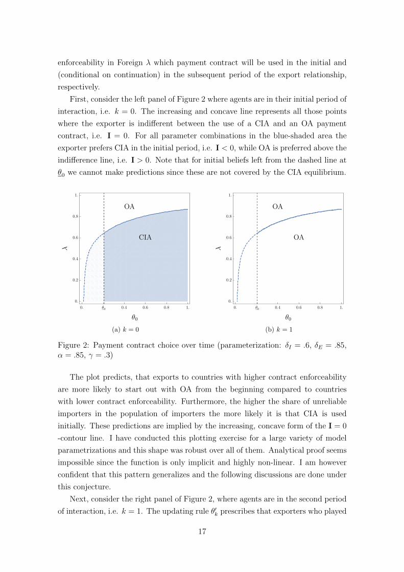
First, consider the left panel of Figure 2 where agents are in their initial period of

interaction, i.e. k = 0. The increasing and concave line represents all those points

where the exporter is indifferent between the use of a CIA and an OA payment

contract, i.e. I = 0. For all parameter combinations in the blue-shaded area the

exporter prefers CIA in the initial period, i.e. I < 0, while OA is preferred above the

indifference line, i.e. I > 0. Note that for initial beliefs left from the dashed line at

θ0 we cannot make predictions since these are not covered by the CIA equilibrium.

(a) k = 0 (b) k = 1

Figure 2: Payment contract choice over time (parameterization: δI = .6, δE = .85,α = .85, γ = .3)

The plot predicts, that exports to countries with higher contract enforceability

are more likely to start out with OA from the beginning compared to countries

with lower contract enforceability. Furthermore, the higher the share of unreliable

importers in the population of importers the more likely it is that CIA is used

initially. These predictions are implied by the increasing, concave form of the I = 0

-contour line. I have conducted this plotting exercise for a large variety of model

parametrizations and this shape was robust over all of them. Analytical proof seems

impossible since the function is only implicit and highly non-linear. I am however

confident that this pattern generalizes and the following discussions are done under

this conjecture.

Next, consider the right panel of Figure 2, where agents are in the second period

of interaction, i.e. k = 1. The updating rule θ′k prescribes that exporters who played

17

CIA initially are, given continuation, sure in k = 1 to be facing a patient type and

choose OA because under full information πΩ > πA. In addition, because of the

concave and increasing shape of the payment contract indifference line all exporters

who played OA already in the initial period continue playing OA. This is because

their belief is updated to θ′1 = θΩ1 which represents a horizontal shift to the left in

the Figure.

In sum, Proposition 3 predicts that if the exporter faces lower costs of capital

than the importer CIA contracts can act as a useful tool in the initial phase of

export relationships. This is particularly pronounced so when the quality of legal

institutions in the destination country is low and the probability of facing unreliable

importers is high. Once an importer has build up a reputation for being reliable OA

contracts will be used across all destination markets. In the following section, we

will study how this result is enriched when exporters have the possibility to ensure

the payment in their open account transactions.

5 Trade credit insurance

With a trade credit insurance (CI) the exporter can rule out the risk of importer

non-payment in an open account transaction. For its service, the insurer charges

a per-transaction fee that we denote by Fk. We assume a perfectly competitive

insurance market and that the fee can be separated into a fixed and a variable

component. It is given by

Fk = m+ δE(1− ΛCIk )Tk, (8)

where the fixed (and time-invariant) component m covers setup and monitoring costs

that the bank incurs for insuring the transaction. The second addend represents the

variable component that depends on the size of the insured transfer in period k, Tk,

which is weighted by the probability of nonpayment 1 − ΛCIk , where ΛCI

k denotes

the probability of payment in the kth period under insurance.5 Finally, because

potential payment default occurs only in t+ 1 the variable component is discounted

by one period.6

Because the insurer has a vital interest that the importer does not default it will

5The formalization of the insurance fee is inspired by Schmidt-Eisenlohr and Niepmann (2016),in particular by their model of the letter of credit contract. However, they do not study thiscontract in a dynamic setting.

6For the discounting we use the exporter’s discount factor. It would be more appropriate to usethe insurer’s own time preference rate here. Because this difference is not of central importancefor the study of the exporter’s insurance decision we abstract from this complicating detail here.

18

engage in importer screening itself before granting a credit insurance.7 We model

this aspect by assuming that starting an export relationship with a trade credit

insurance decreases the proportion of myopic types in the population to θCI = φθ,

where φ ∈ (0, 1) is an inverse measure of the insurer’s ability to screen out myopic

types.

The remainder of the section is structured as follows. In section 5.1 we study

export relationships when the exporter can only choose insured open account as

payment contract. The results bear much resemblance with the open account case

in section 3.2. In part 5.2 we then study how trade credit insurance interacts with

the non-intermediated payment contracts. It thus complements the analysis from

section 4. Finally, in section 5.3 we conduct comparative static exercises.

5.1 Insured payment contracts in isolation

We now study the export relationship when restricted to credit insured payment

contracts. In order to achieve comparability of results we derive an equilibrium that

is based on the same strategy profile as in the open account scenario in section 3.2.

The participation constraints of the importers are the same as in the open ac-

count scenario. Also, the payment incentive constraint for the patient importer is

the same as under open account. The exporter therefore asks the the importer to

transfer the revenue share Tk = βΩR(qk). The exporter thus maximizes in period t:

maxqt

δEβΩR(qt)− cqt − Ft, (9)

which by plugging in Ft can be rewritten as

maxqt

δEΛCIk βΩR(qt)− cqt −m. (10)

Observe that even though the CI eliminates the risk of non-payment the probability

of payment ΛCIk still indirectly affects the exporter’s maximization problem through

the LC-fee. This can be nicely seen when rewriting (9) to (10). For the calculation

of ΛCIk the same mechanics as for the calculation of Λk under open account apply.

However, as described above the exporter beliefs to initially face a myopic type

with smaller probability θCI and the belief of facing a myopic type in period k is

7This assumption is endorsed by the fact that credit insurers such as Euler Hermes and AIGadvertise their insurance services with their expertise in monitoring the reliability of transactioncounterparts.

19

determined via Bayes’ rule as:

θCIk =θCIλk

1− θCI(1− λk).

Consequently, the probability of payment in the kth relationship period under CI is

ΛCIk = 1−θCI(1−λk+1)

1−θCI(1−λk). With this in mind we can solve the maximization problem in

(10). The FOC is:

R′(qt) =c

δEΛCIk βΩ

,

and we denote the resulting, optimal export quantity as QCIk . The payoff in a CI

relationship in the kth transaction then is

πCIk ≡ πCI(θCIk ) = δEΛCIk βΩR(QCI

k )− cQCIk −m. (11)

The following Proposition summarizes our findings on the letter of credit equilib-

rium.

Proposition 4. Suppose only credit insured open account payment contracts are

possible. The exporter starts a partnership whenever he finds a match, maintains

the partnership as long as he does not observe a default, and exports QCIk in the

k-th period of any active partnership. A myopic importer deviates from the contract

whenever she has the opportunity. A patient importer never defaults. Both types

never terminate a partnership. This strategy profile together with the belief updating

rule θCIk is a sequential equilibrium.

When all uncertainty about the importer’s type is resolved, equation (11) can

be written as

πCI ≡ πCI(θCIk = 0) = δEβΩR(QΩ)− cQΩ −m = πΩ −m

which shows that πΩ > πCI . This gives the following Corollary.

Corollary 1. Under complete information, insured open account payment con-

tracts are strictly dominated by non-insured open account contracts.

The corollary hints at a result that we will derive in the following when studying

the interaction of credit insurances with the other contract forms: Once the exporter

attains enough information about the importer’s type it will be better for him to

conduct his transactions through open account instead of insuring it.

20

5.2 When to employ trade credit insurance

In this section, we study the payment contract decision when the choice set now also

includes the possibility to insure the OA transaction. We denote the extended choice

set by F+ ≡ CIA,OA,CI. Because of the independence axiom from expected

utility theory we can analyze the payment contract decision in two separate cases:

i) We study under which conditions CI is preferred to OA (and vice versa) given

that OA is preferred to CIA, i.e. expression (5) holds. ii) We study under which

conditions CI is preferred to CIA (and vice versa) given that CIA is preferred to

OA, i.e. expression (5) does not hold.

First, consider case i) and let us determine under which conditions we will choose

CI instead of OA. The respective belief updating rules θCIk and θΩk are very similar.

Their only difference is that the prior probability of being matched with a myopic

type under CI is downsized by the factor φ. Note that we can write the belief under

OA for period k + 1 as θΩk+1 =

θΩk λ

1−θΩk (1−λ)

and that this is an increasing and strictly

convex function of θΩk . As a consequence, given (5), the incentives to employ a credit

insured contract are always largest in the initial period of interaction because the

exporter’s learning effect through the screening activity of the insurer is largest.

Hence, whenever CI is employed instead of OA it will for sure be employed in the

initial transaction. Note also, that since the learning about the importer through

insurer screening is permanent, the exporter will not employ CI for more than the

initial period.8 Consequently, the exporter decides for a credit insurance in an export

relationship if and only if the payoffs from using a CI in the initial period and OA

forever after are larger than the payoffs obtained from using OA in every period.

Formally,

πCI0 +∞∑k=1

δkπΩ(θCIk ) >∞∑k=0

δkπΩ(θΩk ).

This expression can be rearranged to:

∞∑k=0

δk[πΩ(θCIk )− πΩ(θΩ

k )]> m, (12)

which intuitively means that CI is employed (and only so in the initial period) if the

continued benefits from importer screening through the insurer are larger than the

fixed costs of the one-period insurance contract m.

Next, consider case ii) and let us determine under which conditions we will choose

CI instead of CIA. The problem simplifies by recognizing that after one period of

8This is implied by our assumption of only two types of importers and that their type is constant.

21

CI it is dominated by OA. In addition, switching from CIA to CI is never profitable

because the exporter will have complete knowledge of the importer type after the

first CIA transaction (which leads to OA by Corollary 1). Hence, if the exporter

uses CI in the present scenario he will do it only in the initial transaction. CI is

preferred to CIA in the initial period if and only if:

πCI0 + δEπA(θCI1 ) +

δ2E

1− δEπΩ ≥ πA(θΩ

0 ) +δE

1− δEπΩ.

The equation can be simplified to:

πCI0 − πA(θΩ0 ) > δE

[πΩ − πA(θCI1 )

](13)

The following Proposition gives a complete summary for every period and beliefs in

the export relationship which payment contract will be used:

Proposition 5. An exporter will consider to conduct a transaction through credit

insurance only if in the initial period of an export relationship. This transaction will

be conducted with CI if and only if either of the following is true:

a) (5) holds and (12) holds, or

b) (5) does not hold and (13) holds.

All later periods of the export relationship are captured entirely through expression

(5).

Because it is more illustrative, in analogy to section 4.2, we conduct the discus-

sion of the results for the case of a parameterized revenue function. The following

Corollary restates the differences in Proposition 5 when using the revenue function

from before.

Corollary 2. Suppose that R(q) = q1−α

1−α . Then the exporter conducts the initial

transaction with CI if and only if either of the following is true:

a) I > 0 holds and J ≡∑∞

k=0 δk[(ΛCI

k )1α − (Λk)

1α

]− κ > 0, or

b) I < 0 and K ≡ (ΛCI0 )

1α − δE − κ +

(δI

δEβΩ

) 1α [δE(1− θCI1 )− (1− θΩ

0 )]> 0

holds.9

9Without loss of generality we define and use m ≡ κπΩ, κ > 0, since πΩ = (δEβΩ)

1α c

α−1α

α1−α is

a constant.

22

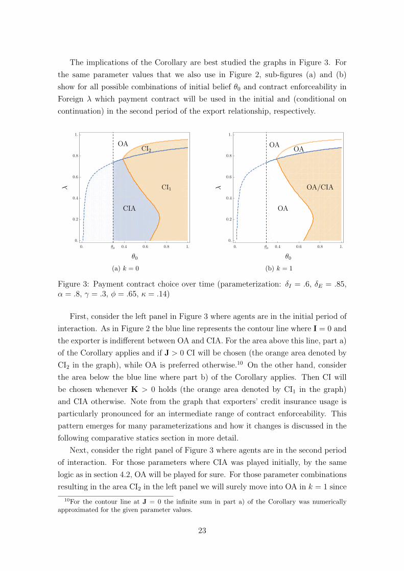
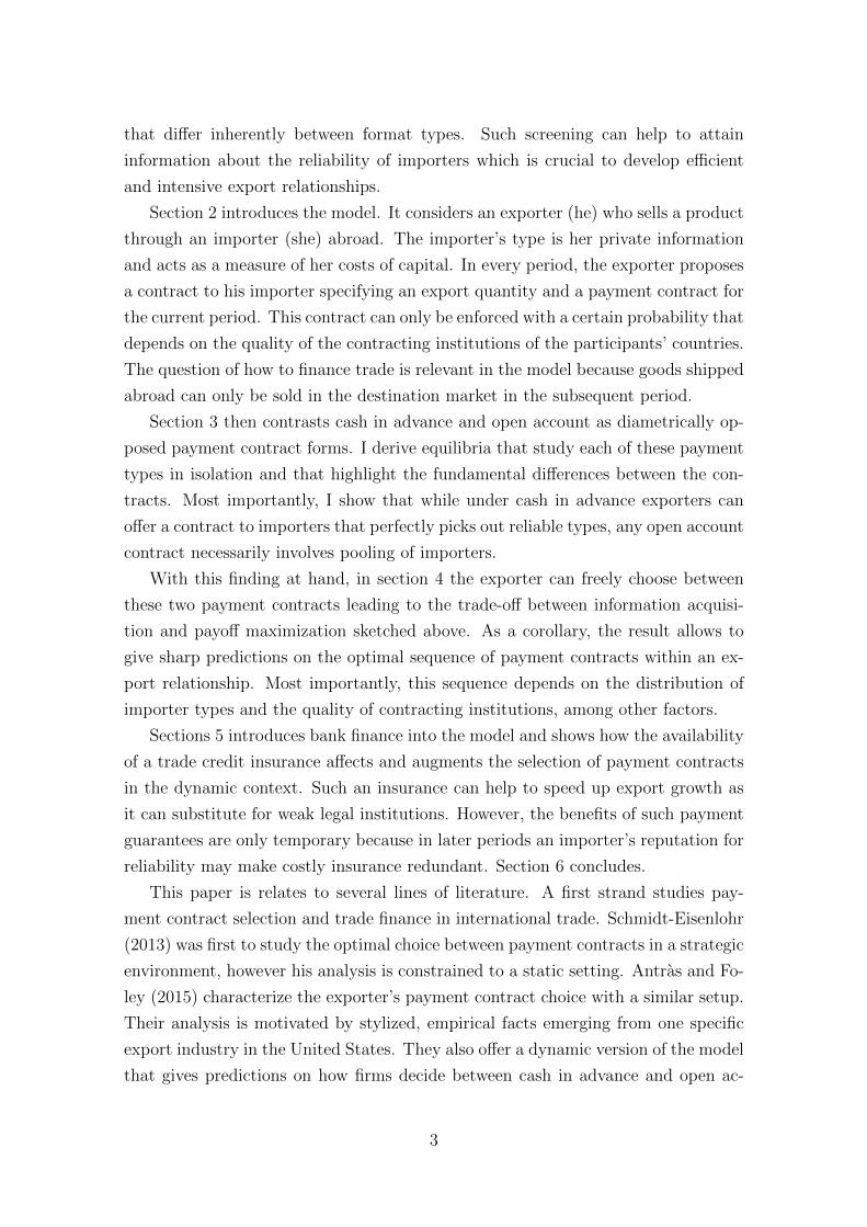
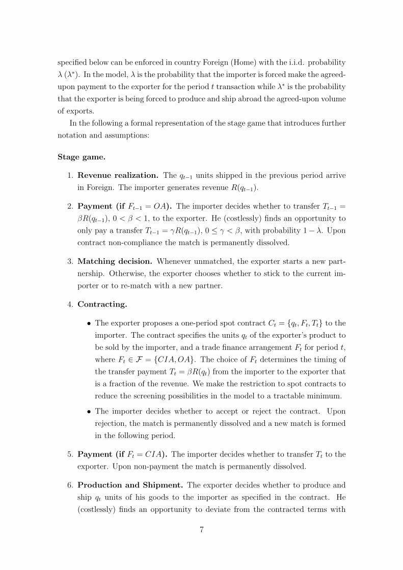
The implications of the Corollary are best studied the graphs in Figure 3. For

the same parameter values that we also use in Figure 2, sub-figures (a) and (b)

show for all possible combinations of initial belief θ0 and contract enforceability in

Foreign λ which payment contract will be used in the initial and (conditional on

continuation) in the second period of the export relationship, respectively.

(a) k = 0 (b) k = 1

Figure 3: Payment contract choice over time (parameterization: δI = .6, δE = .85,α = .8, γ = .3, φ = .65, κ = .14)

First, consider the left panel in Figure 3 where agents are in the initial period of

interaction. As in Figure 2 the blue line represents the contour line where I = 0 and

the exporter is indifferent between OA and CIA. For the area above this line, part a)

of the Corollary applies and if J > 0 CI will be chosen (the orange area denoted by

CI2 in the graph), while OA is preferred otherwise.10 On the other hand, consider

the area below the blue line where part b) of the Corollary applies. Then CI will

be chosen whenever K > 0 holds (the orange area denoted by CI1 in the graph)

and CIA otherwise. Note from the graph that exporters’ credit insurance usage is

particularly pronounced for an intermediate range of contract enforceability. This

pattern emerges for many parameterizations and how it changes is discussed in the

following comparative statics section in more detail.

Next, consider the right panel of Figure 3 where agents are in the second period

of interaction. For those parameters where CIA was played initially, by the same

logic as in section 4.2, OA will be played for sure. For those parameter combinations

resulting in the area CI2 in the left panel we will surely move into OA in k = 1 since

10For the contour line at J = 0 the infinite sum in part a) of the Corollary was numericallyapproximated for the given parameter values.

23

for the previously discussed reasons no further value can be attained from continuing

to insure the transaction. The behavior of exporters starting a relationship in area

CI1 is more intricate. Surely, they will not engage in CI anymore for the same reasons

as in the first case. However, depending on the belief θCI1 , they might either conduct

the transaction through OA or CIA. If OA is employed the exporter will continue

to use OA for any subsequent period since the (I = 0)-contour line is increasing and

concave. If CIA is used then the exporter will switch to OA from k = 2 onwards.

Generally, we can conclude that for any combination of parameters a transaction

will be conducted via open account for k ≥ 2.

To sum up, Proposition 5 predicts that trade credit insurances can act as a

valuable tool in the initial phase of export relationships when the importer’s ex-

pected reliability is low. The graphs in Figure 3 (as well as the robustness-checks in

the following subsection) suggest that the usage of credit insurances is particularly

pronounced for intermediate qualities of contracting institutions. An intuitive ra-

tionalization for this pattern is that credit insurance is particularly attractive when,

on the one side, insurance is not too expensive. It could be too costly because of

the high risk of expropriation at low values of λ. On the other side, its value is po-

tentially marginalized when facing strong legal institutions at high λ. Empirically,

this pattern finds traction through the results by Schmidt-Eisenlohr and Niepmann

(2016) who report for the U.S. that letter of credit insurances matter most for ex-

ports to countries with intermediate levels of risk.11 The analysis shows that while

exporters can initially benefit from the insurer’s screening abilities once importers

have build up a reputation for reliability, behavior will converge towards OA that

in the medium- and long-run yields the largest flow payoffs.

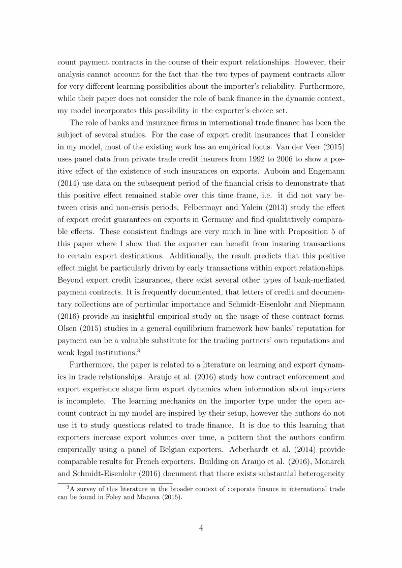
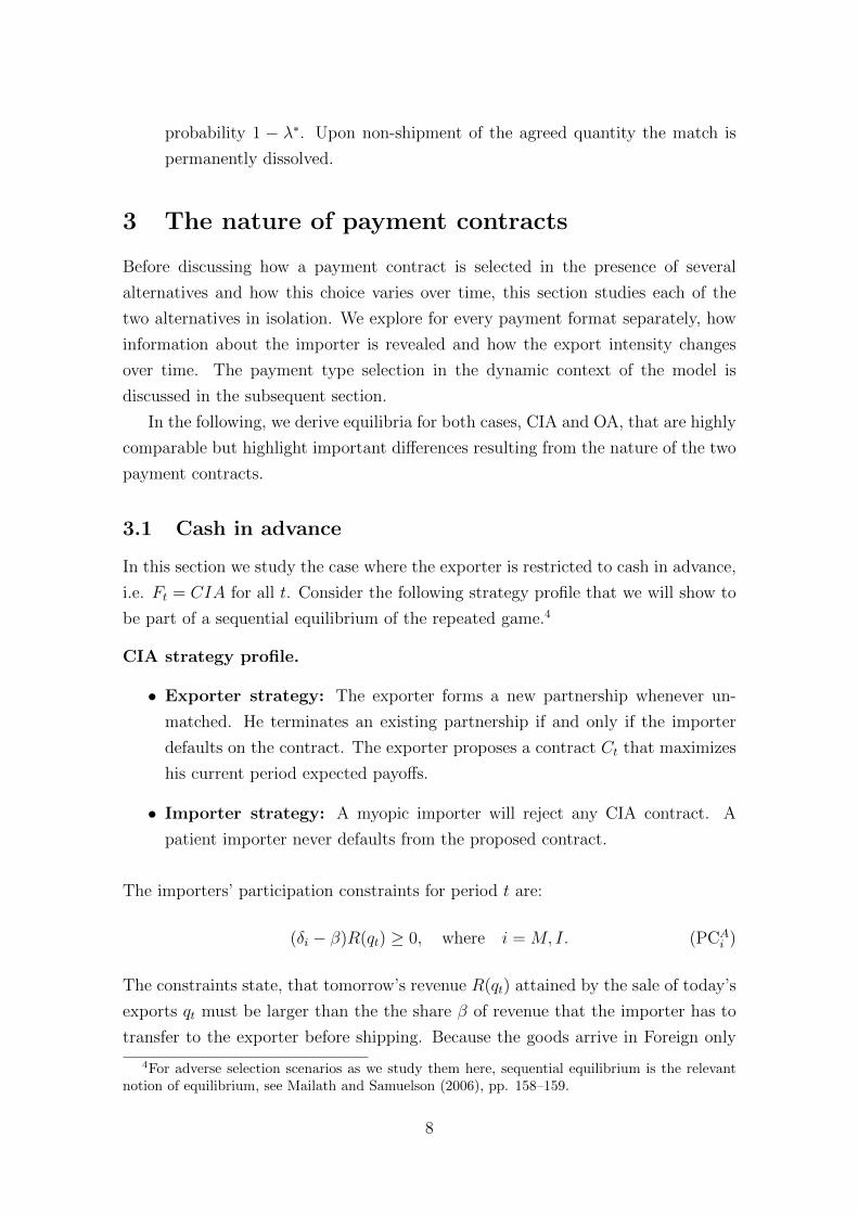
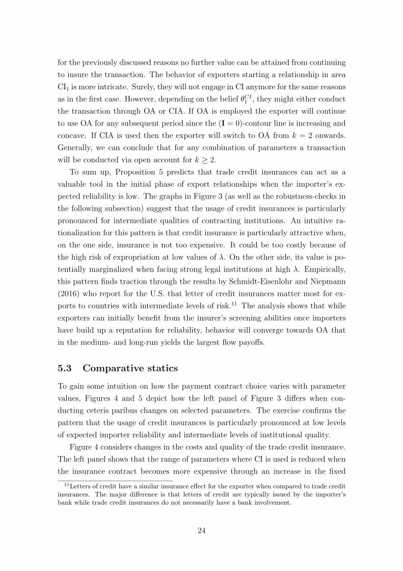
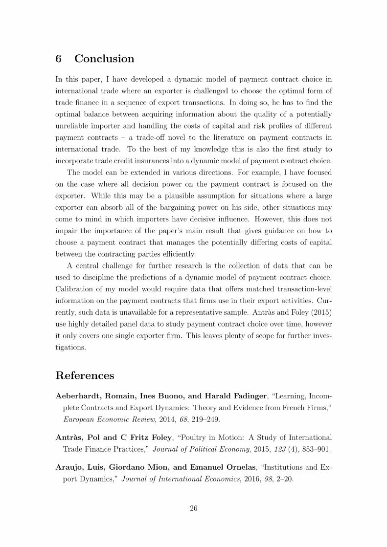
5.3 Comparative statics

To gain some intuition on how the payment contract choice varies with parameter

values, Figures 4 and 5 depict how the left panel of Figure 3 differs when con-

ducting ceteris paribus changes on selected parameters. The exercise confirms the

pattern that the usage of credit insurances is particularly pronounced at low levels

of expected importer reliability and intermediate levels of institutional quality.

Figure 4 considers changes in the costs and quality of the trade credit insurance.

The left panel shows that the range of parameters where CI is used is reduced when

the insurance contract becomes more expensive through an increase in the fixed

11Letters of credit have a similar insurance effect for the exporter when compared to trade creditinsurances. The major difference is that letters of credit are typically issued by the importer’sbank while trade credit insurances do not necessarily have a bank involvement.

24

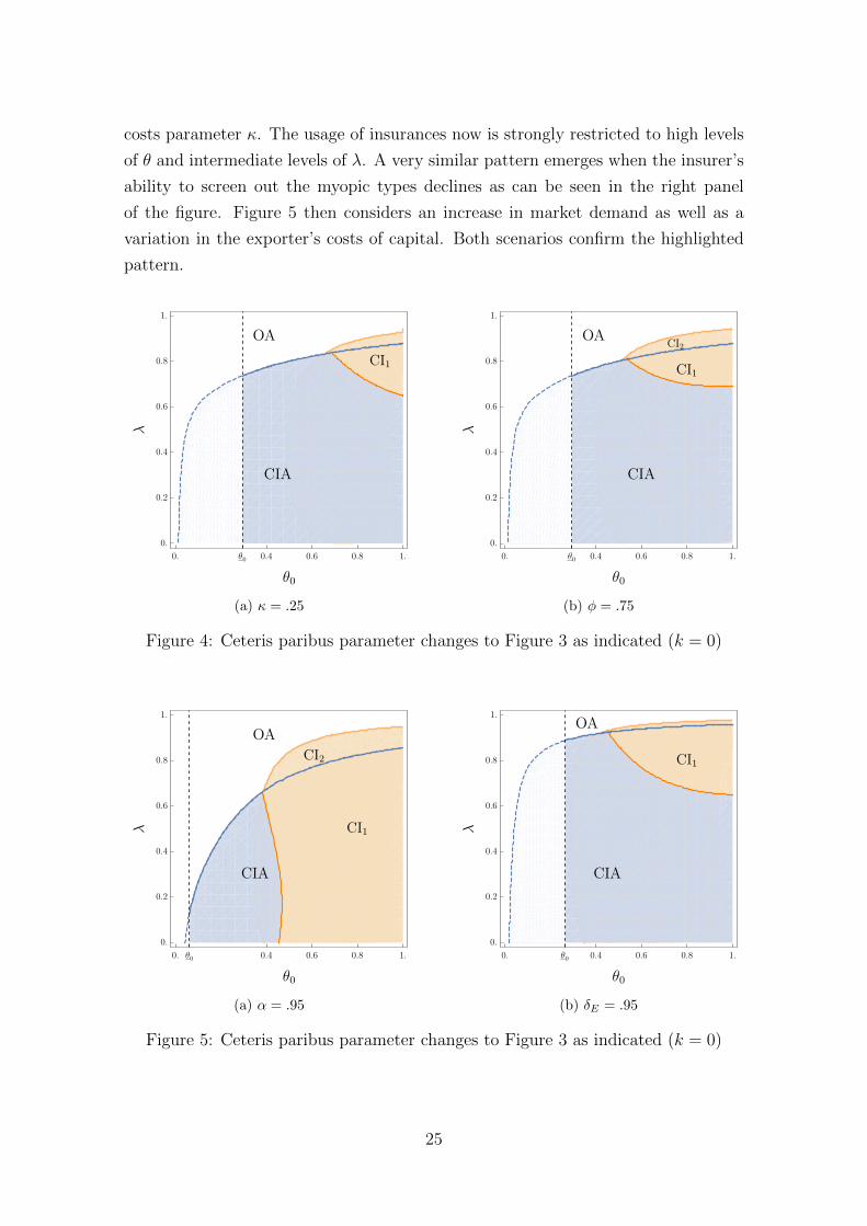
costs parameter κ. The usage of insurances now is strongly restricted to high levels

of θ and intermediate levels of λ. A very similar pattern emerges when the insurer’s

ability to screen out the myopic types declines as can be seen in the right panel

of the figure. Figure 5 then considers an increase in market demand as well as a

variation in the exporter’s costs of capital. Both scenarios confirm the highlighted

pattern.

(a) κ = .25 (b) φ = .75

Figure 4: Ceteris paribus parameter changes to Figure 3 as indicated (k = 0)

(a) α = .95 (b) δE = .95

Figure 5: Ceteris paribus parameter changes to Figure 3 as indicated (k = 0)

25

6 Conclusion

In this paper, I have developed a dynamic model of payment contract choice in

international trade where an exporter is challenged to choose the optimal form of

trade finance in a sequence of export transactions. In doing so, he has to find the

optimal balance between acquiring information about the quality of a potentially

unreliable importer and handling the costs of capital and risk profiles of different

payment contracts – a trade-off novel to the literature on payment contracts in

international trade. To the best of my knowledge this is also the first study to

incorporate trade credit insurances into a dynamic model of payment contract choice.

The model can be extended in various directions. For example, I have focused

on the case where all decision power on the payment contract is focused on the

exporter. While this may be a plausible assumption for situations where a large

exporter can absorb all of the bargaining power on his side, other situations may

come to mind in which importers have decisive influence. However, this does not

impair the importance of the paper’s main result that gives guidance on how to

choose a payment contract that manages the potentially differing costs of capital

between the contracting parties efficiently.

A central challenge for further research is the collection of data that can be

used to discipline the predictions of a dynamic model of payment contract choice.

Calibration of my model would require data that offers matched transaction-level

information on the payment contracts that firms use in their export activities. Cur-

rently, such data is unavailable for a representative sample. Antras and Foley (2015)

use highly detailed panel data to study payment contract choice over time, however

it only covers one single exporter firm. This leaves plenty of scope for further inves-

tigations.

References

Aeberhardt, Romain, Ines Buono, and Harald Fadinger, “Learning, Incom-

plete Contracts and Export Dynamics: Theory and Evidence from French Firms,”

European Economic Review, 2014, 68, 219–249.

Antras, Pol and C Fritz Foley, “Poultry in Motion: A Study of International

Trade Finance Practices,” Journal of Political Economy, 2015, 123 (4), 853–901.

Araujo, Luis, Giordano Mion, and Emanuel Ornelas, “Institutions and Ex-

port Dynamics,” Journal of International Economics, 2016, 98, 2–20.

26

Auboin, Marc and Martina Engemann, “Testing the Trade Credit and Trade

Link: Evidence from Data on Export Credit Insurance,” Review of World Eco-

nomics, 2014, 150 (4), 715–743.

Baker, George, Robert Gibbons, and Kevin J Murphy, “Relational Con-

tracts and the Theory of the Firm,” The Quarterly Journal of Economics, 2002,

117 (1), 39–84.

Besedes, Tibor, “A Search Cost Perspective on Formation and Duration of Trade,”

Review of International Economics, 2008, 16 (5), 835–849.

Board, Simon and Moritz Meyer ter Vehn, “Relational Contracts in Compet-

itive Labour Markets,” The Review of Economic Studies, 2015, 82 (2), 490–534.

Chassang, Sylvain, “Building Routines: Learning, Cooperation, and the Dynam-

ics of Incomplete Relational Contracts,” American Economic Review, 2010, 100

(1), 448–465.

Defever, Fabrice, Christian Fischer, and Jens Suedekum, “Relational Con-

tracts and Supplier Turnover in the Global Economy,” Journal of International

Economics, 2016, forthcoming.

der Veer, Koen JM Van, “The Private Export Credit Insurance Effect on Trade,”

Journal of Risk and Insurance, 2015, 82 (3), 601–624.

Egan, Mary Lou and Ashoka Mody, “Buyer-Seller Links in Export Develop-

ment,” World Development, 1992, 20 (3), 321–334.

Felbermayr, Gabriel J and Erdal Yalcin, “Export Credit Guarantees and Ex-

port Performance: An Empirical Analysis for Germany,” The World Economy,

2013, 36 (8), 967–999.

Foley, C Fritz and Kalina Manova, “International Trade, Multinational Activ-

ity, and Corporate Finance,” Annual Review of Economics, 2015, 7 (1), 119–146.

Halac, Marina, “Relational Contracts and the Value of Relationships,” American

Economic Review, 2012, 102 (2), 750–779.

ITA, “Trade Finance Guide: A Quick Reference for Exporters,” U.S. Department

of Commerce: International Trade Administration 2007.

Levin, Jonathan, “Relational Incentive Contracts,” American Economic Review,

2003, 93 (3), 835–857.

27

Mailath, George J and Larry Samuelson, Repeated Games and Reputations:

Long-Run Relationships, Oxford University Press, 2006.

Monarch, Ryan and Tim Schmidt-Eisenlohr, “Learning and the Value of Trade

Relationships,” Working Paper 2016.

Olsen, Morten, “How Firms Overcome Weak International Contract Enforcement:

Repeated Interaction, Collective Punishment, and Trade Finance,” Working Pa-

per 2015.

Rauch, James E and Joel Watson, “Starting Small in an Unfamiliar Environ-

ment,” International Journal of Industrial Organization, 2003, 21 (7), 1021–1042.

Schmidt-Eisenlohr, Tim, “Towards a Theory of Trade Finance,” Journal of In-

ternational Economics, 2013, 91 (1), 96–112.

and Friederike Niepmann, “International Trade, Risk and the Role of Banks,”

Working Paper 2016.

Thomas, Jonathan and Tim Worrall, “Foreign Direct Investment and the Risk

of Expropriation,” The Review of Economic Studies, 1994, 61 (1), 81–108.

Yang, Huanxing, “Nonstationary Relational Contracts with Adverse Selection,”

International Economic Review, 2013, 54 (2), 525–547.

APPENDIX

Proof of Lemma 1

At the Production and Shipment stage of any period k of any export relationship

the exporter will not deviate from the contract if and only if:

−cQA+δE

1− δEπA ≥ (1−λ∗)

(δEπ

A0 +

δ2E

1− δEπA)

+λ∗(−cQA +

δE1− δE

πA)

(14)

Equation (14) states that making the effort to produce the contracted output plus

the future payoff from continuing the current export relationship (where the exporter

can be sure to interact with a patient type) must result in a higher payoff than devi-

ating by not producing and shipping the agreed quantity QA. Note that deviation is

28

possible only if contracts cannot be enforced which happens with probability 1−λ∗.Simplification of (14) gives:

δE ≥cQA

θ0πA≡ δE (15)

Observe that the equilibrium does exist if and only if δE < 1. Consequently, a

necessary and sufficient condition for existence is θ0 >cQA

πA.

Observe that the proof holds for every relationship period and not only for k =

0 because deviation implies re-matching. This is the case, because the importer

anticipates to again not receive the goods in the following transaction with again

leads to a loss for her. It is therefore better for her to terminate the relationship.

Hence, the exporter must re-match.

Proof of Lemma 2

At the Payment stage of any period t + 1 it is incentive compatible for the patient

importer to transfer the contracted share β of the revenue R(qt) if and only if:

−βR(qt)+(1−β)∞∑

k=t+1

δk−tI R(qk) ≥ λ

(−βR(qt) + (1− β)

∞∑k=t+1

δk−tI R(qk)

)−(1−λ)γR(qt)

Simplifying gives:

(1− β)∞∑

k=t+1

δk−tI R(qk) ≥ (β − γ)R(qt) (16)

Note, that Λk → 1 for k →∞ which implies that the optimal export quantity QΩk

under open account and therefore revenue R(QΩk ) are increasing with relationship

duration k. This observation allows us to derive a simple expression for the incentive

compatible transfer share β from (16). Observe that the deviation incentive is largest

in the limit (for relationship length k → ∞) and denote the associated export

quantity by QΩ. We can rewrite the IC-constraint to:

t→∞ : (1− β)δI

1− δIR(QΩ) ≥ (β − γ)R(QΩ) ⇔ β ≤ δI + γ(1− δI) (ICΩ

I )

If (ICΩI ) holds, the patient importer will never deviate from the contract no matter

how large the exported volume under open account.

29

When the importer is more patient than the exporter

Noting that CIA now leads to larger flow payoffs than OA under full information

we can derive by steps analogue to the main text a result equivalent to Proposition

3 but which now covers the case when δI > δEβΩ. This yields:

Proposition 3’. Suppose that δI > δEβΩ. Consider the kth transaction in an

export relationship. The exporter will conduct this transaction through Open Account

if and only if

πΩk − πA(θΩ

k ) ≥ δE[πA − πA(θΩ

k+1)]

(17)

and ask for Cash in Advance otherwise.

The result gives the following behavioral predictions. Suppose that parameters

are such that the initial transaction of the export relationship is conducted through

CIA, i.e. expression (17) does not hold. Then any subsequent transaction with the

same importer will be conducted through CIA as well since πA > πΩ. Therefore

no switching between contracts occurs. On the other side, suppose that OA is

played initially which can be the case when πΩ0 > πA0 (and additionally, (17) holds).

However, because πA > πΩ it must be the case that in some k behavior will switches

to CIA and then stays there forever.

30