Patrolling Public Schools:The Impact of Funding for School Police on Student

Discipline and Long-term Education Outcomes

Emily K. Weisburst∗

October 2018

AbstractAs police officers have become increasingly common in U.S. public schools, their role

in school discipline has often expanded. While there is growing public debate aboutthe consequences of police presence in schools, there is scant evidence of the impactof police on student discipline and academic outcomes. This paper provides the firstquasi-experimental estimate of funding for school police on student outcomes, leveragingvariation in federal Community Oriented Policing Services (COPS) grants. Exploitingdetailed data on over 2.5 million students in Texas, I find that federal grants for policein schools increase middle school discipline rates by six percent. Further, I find thatlow-income students and Black and Hispanic students experience the largest increasesin discipline. I also find that exposure to a three-year federal grant for school police isassociated with a 2.5 percent decrease in high school graduation rates and a four percentdecrease in college enrollment rates.

JEL Classification: H76, J24, I28, K42Keywords: School Discipline, School Resource Officers, Police, Community Oriented Policing Services(COPS)

The views in this study are the result of independent research and do not necessarily reflect the viewsof the Texas Education Research Center, the Texas Education Agency, the Texas Higher EducationCoordinating Board or the Texas Workforce Commission. This project was supported by a NationalAcademy of Education Spencer Dissertation Fellowship grant.

∗Luskin School of Public Affairs, Department of Public Policy, University of California, Los Angeles. Con-tact: weisburst@ucla.edu. I am grateful to Professors Sandra Black, Jason Abrevaya, Leigh Linden, BeckyPettit, Steve Trejo, Marika Cabral, Rich Murphy, and Mike Geruso, as well as the seminar participants atthe University of Texas at Austin for their helpful comments and feedback. The views in this study arethe result of independent research and do not necessarily reflect the views of the Texas Education ResearchCenter, the Texas Education Agency, the Texas Higher Education Coordinating Board or the Texas Work-force Commission. This research was supported by a National Academy of Education Spencer DissertationFellowship.

1

1 INTRODUCTION

Police are an active presence in U.S. public schools. In 2014, 43 percent of all public schools

had security staff at school at least once a week, affecting over 70 percent of students across

the country (Zhang et al., 2016). While estimates vary, government surveys suggest that there

are at least 20,000 police officers working in schools (James and McCallion, 2013). In the

wake of recent high-profile school shooting incidents, there are new plans to escalate police

presence in public schools at the local and national level (e.g. DOJ, 2018; Perano and Ellis,

2018).

School Resource Officers (SROs) serve a number of roles, including protecting campuses

from outside threats and educating students about safety and the law. However, SROs

can also fill another role: They can engage in daily school discipline issues and administer

punishments for student behavior. Despite the fact that reported crimes against students have

decreased in recent decades, suspensions and expulsions have become more commonplace,

increasing by nearly 200 percent between 2000 and 2014, and affecting Hispanic and Black

students at 1.5 to over three times the rate of White students (DeVoe et al., 2003; OCR, 2014;

Zhang et al., 2016).

As police have become a fixture in public schools, policy-makers, educators, and re-

searchers are debating the merits of this approach to school discipline. Proponents of school

police advocate that SROs are critical to establishing safe school environments and serve as

educators, counselors, and positive role models for students (Canady et al., 2012).1 Crit-

ics of school police argue that SROs can instead create a heavy-handed disciplinary culture

1These roles are referred to as the Triad model of SRO responsibility, as educators, informal counselors,and law enforcement officers. This model advises against SRO involvement in routine school discipline matters(Canady et al., 2012).

2

that adversely affects learning and may further disadvantage poor and minority students in

low-performing schools (Balko, 2018).

Using data on over 2.5 million public-school students in Texas, I find that federal

funding for school police increases disciplinary rates for middle school students by six percent

but does not change high school disciplinary rates. I also examine second-order effects on

long-term educational outcomes and find suggestive evidence that exposure to a three-year

federal grant for school police decreases high school graduation rates by approximately 2.5

percent and college enrollment rates by four percent.

I find that the impact of police funding differs across student race and socioeconomic

status. While all student race and income groups display significant increases in disciplinary

actions, the effects are largest for low-income students and Black and Hispanic students.

These results are consistent with work that finds that school disciplinary policies have a

disparate impact on poor students and minority students. The results imply that the effects

of expansions in school police may be most pronounced for marginalized student groups.

2 LITERATURE REVIEW

School discipline policy has the potential to have real impacts on academic success and ed-

ucational attainment. Safety is a prerequisite to learning, and policies that increase school

safety and deter dangerous or disruptive behavior may have a positive effect on student aca-

demic success. A small number of survey studies find that students have relatively positive

perceptions of SROs and believe they increase school safety (e.g. Raymond, 2010; Brown and

Benedict, 2005). Likewise, bullying and aggressive behavior can inflict serious psychological

3

harm on student victims and SROs may be capable of reducing in-school bullying (Ttofi and

Farrington, 2011; Wilson and Lipsey, 2007).

Alternatively, disciplinary actions may stigmatize disciplined students and decrease

their attachment to school, negatively affecting their performance (Steinberg and Lacoe, 2017;

Wald and Losen, 2003; Mendez, 2003). Studies in economics have found that juvenile arrests

and juvenile detention decrease the probability of completing high school and increase the

probability of future arrests (Aizer and Doyle, 2015; Kirk and Sampson, 2011; Hjalmarsson,

2008). The economic literature on juvenile behavioral responses to criminal sanctions has

also found that juveniles may be less deterred by changes in punishment severity (Lee and

McCrary, 2009) and may be more negatively impacted by the experience of sanctions (Aizer

and Doyle, 2015; Bayer et al., 2009). By extension, school discipline, citations, arrests, or

referrals to juvenile detention may lead to future involvement with the criminal justice system,

in a process often termed the "school-to-prison pipeline" (Wald and Losen, 2003). Further,

if students obtain a criminal record for offenses in school, they may face future barriers to

employment (Pager et al., 2009).2

Through these channels, school police can positively or negatively impact the educa-

tional attainment of the students that they interact with, potentially affecting their human

capital development, labor market attachment, and earnings later in life (Hanushek and

Welch, 2006). This is the first study to estimate the impact of funding for school police on

student disciplinary and education outcomes using quasi-experimental quantitative methods.

There is a large qualitative and ethnographic literature that documents the growth of

harsh school sanctions policies and their disparate impact on low-income minority students2Juveniles with criminal records can also face restricted eligibility for federal grants and loans for college,

increasing the barriers to enrollment (Lovenheim and Owens, 2014).

4

(e.g. Nolan, 2011; Kupchik, 2010; Devine, 1996). This work has found that administrators’

and teachers’ roles in school discipline and classroom management are increasingly outsourced

to SROs, and that SROs not only utilize their ability to arrest students for criminal offenses,

but frequently participate in school discipline matters such as code of conduct violations

(Kupchik, 2010).

However, literature reviews and meta-analysis studies note the lack of quantitative

empirical evidence evaluating the impact of school police (Steinberg and Lacoe, 2017; James

and McCallion, 2013; Fisher and Hennessy, 2016; Addington, 2009; Brown, 2006; Finn and

McDevitt, 2005). Studies in this space have often been limited by small samples or consider

simple observational pre-post or cross-sectional comparisons between schools.3

A recent paper by Owens (2017) is a notable exception; it examines the impact of

changes in police hiring on arrests in and out of school for students of different ages using

national data at the police department and county-level. Similar to the current study, Owens

(2017) estimates her model using quasi-experimental variation in federal Community Oriented

Police Services (COPS) grant funding for school police. She finds that expansions in school

police increase property and violent arrests for children younger than high school age on school

grounds and increase drug arrests for high school aged juveniles off of school grounds. Owens

(2017) finding of increases in in-school arrest rates for younger students is consistent with

the finding in this study that funding for school police increases middle school disciplinary

actions. I build upon Owens’ work by exploring the academic ramifications of school police

using detailed student-level data. I am able to examine the impact of grants for school police

3An example of descriptive research in this area is Na and Gottfredson (2011), which uses a survey of 470schools and a difference-in-differences design, and finds that schools that increase policing report an increasein non-serious violent crimes.

5

on student disciplinary actions, high school graduation and college enrollment, as well as how

these effects vary for students in different demographic groups.

Studying the impact of school police presence on students has proved difficult for a

number of reasons. First, appropriate data is hard to obtain. While schools follow a mandate

to track aggregate disciplinary outcomes, detailed student-level data sets are not widely avail-

able. More importantly, information on the number of police employed in particular school

districts is not uniformly tracked because SROs are typically employed by a third-party police

department rather than directly by a school district. Beyond data constraints, the assignment

of police officers to particular schools and districts is designed by school administrators, city

officials, and law enforcement leaders and is non-random. School districts with higher rates

of students in poverty, higher minority populations, higher levels of disciplinary actions, and

lower graduation rates typically have a larger police presence (Kupchik and Ward, 2014).

Given these selected characteristics, cross-sectional comparisons between school districts that

have police and those that do not will be biased. However, even when researchers examine

changes in police presence in a particular school district, the timing of investments in police

may also be a function of changes in discipline and student behavior Owens (2017).4 If school

districts choose to hire police when they experience an increase in negative student behaviors,

then not only is discipline a function of policing but policing is also a function of discipline.

In this setting, simple longitudinal or panel data analysis will be biased by simultaneity.

I use information on federal COPS grants to fund police in public schools to address

these measurement obstacles. I measure the impact of these grants on a range of student

4Literature in economics and criminology has shown the importance of accounting for simultaneity inpolice presence and crime rates (Nagin, 2013). A growing body of economics research using quasi-experimentalmethods that finds that increasing police presence reduces crime rates in the general population (e.g. DeAngeloand Hansen, 2014; Draca et al., 2011; Lin, 2009; Klick and Tabarrok, 2005; Di Tella and Schargrodsky, 2004).

6

outcomes, using variation across years within school districts, rather than cross-sectional

variation across school districts. Within a given district, I compare disciplinary outcomes for

students enrolled in years when the district receives federal grant funding to students enrolled

in years without this funding. I also adapt this model to consider secondary effects on high

school graduation and college enrollment, by examining the impact of differences in exposure

to grants across student cohorts within school districts.

Critically, I also account for non-random school district decisions to seek funding for

police in particular years by including grant application timing as a direct control in the

model.5 This strategy complements and builds on Owens (2017), whose paper uses variation

in the size of grant awards for school police but does not control for school district grant

application decisions.

3 INSTITUTIONAL CONTEXT

3.1 Federal COPS Grants for School Police

The COPS office at the Department of Justice (DOJ) was originally established to fund the

hiring of new police officers as part of the Violent Crime Control Act of 1994. In 1998, the

COPS office extended its grant programs to include funding for schools, with the launch of

pilot programs to fund SRO hiring and partnerships between police departments, schools,

and other community organizations.

Political interest school police escalated after the high-profile Columbine school shoot-

5The empirical approach in this study is closely related to work on the impact of COPS hiring grantsfor traditional police departments on municipal crime rates (Weisburst, 2017). Likewise, this paper is alsorelated to the larger literature on the impact of COPS grants on crime (Evans and Owens, 2007; GAO, 2005;Zhao et al., 2002).

7

ing in 1999. Prior to 1999, school police were primarily confined to large urban districts

(Addington, 2009; Brown, 2006).6 Early school police programs were linked to policies of

"zero-tolerance" toward student misconduct in the 1980s and 1990s.7 Over the past two

decades, new SRO programs have been founded while pre-existing SRO programs have grown;

today, there are at least 20,000 SROs nationwide and over 70 percent of students attend

schools with security staff on campus at least once a week (Zhang et al., 2016; James and Mc-

Callion, 2013). Policy-makers have invested in school police with the aims of both preventing

tragic school shootings and generally improving safety in public schools.

Since Columbine, political support for COPS school grants has fluctuated. Federal

appropriations for COPS school grants declined in the mid-2000s as part of a broader reduc-

tion in COPS funding by the Bush Administration, which had concerns about the overall

effectiveness of the grants (Evans and Owens, 2007). During the Obama Administration,

officials became increasingly concerned about the active role many SROs play in disciplining

students, the large disparity in school discipline by student race, and the fact that student

interactions with SROs may have repercussions for student involvement in the criminal justice

system later in life. Given these concerns, COPS funding levels for school police declined in

2009. In 2014 and 2016, the Departments of Education and Justice released new guidance

and resources for SRO programs, defining a narrow role for school police that excludes in-

volvement in routine discipline and highlights the importance of disciplinary systems that do

6A sampling of the earliest records of police operating in public schools are Los Angeles, CA (1948),Indianapolis, CA (1939), and Flint, MI (early 1950s). The National Association of School Resource Officers(NASRO) was established in 1991, also prior to the expansion of school police that was spurred by theColumbine shooting (Brown, 2006).

7"Zero-tolerance" policies refer to laws or school policies that require predetermined consequences forspecific student offenses, without considering mitigating circumstances or context for an offense incident.Recent work by Curran (2016) examines state "zero-tolerance" statutes and finds that these polices modestlyincrease overall suspension rates and have larger impacts on Black students.

8

not discriminate against groups of students (Steinberg and Lacoe, 2017; EOP, 2016). In a

reversal of this approach, the Trump Administration has considered revoking this guidance

and has introduced plans to increase funding for COPS school grants (DOJ, 2018; Camera,

2017).

During the sample period of this paper, 1999 to 2008, there were three broad groups

of federal grants available for use in schools. This paper focuses on the impact of the largest

program, COPS in Schools (CIS), which provided up to $125,000 in hiring funds per SRO

over a period of three years. Approximately three-quarters of all COPS funding for school

security has been granted through CIS. The COPS office has also funded additional grants for

school security that are broader and more flexible in scope, Secure Our Schools (SOS) grants,

school-based partnerships (SBP), the Safe Schools Initiative (SSI), as well as other program

grants for school district police departments. I focus on the CIS program because of its size

and articulated goal to increase police officer presence in public schools. While CIS grants

are the primary focus of the paper, I include controls for other COPS school grant programs

in the empirical model.8

The application process for CIS grants is narrative-based. Each applicant is asked to

describe safety problems facing their school district and their proposed approach to remedying

these problems, denote any community partnerships that support the grant proposal, and

state their request for assistance. Review of these applications is based on the subjective

judgements of individuals at the COPS office. It is likely that grant awardees were not

randomly selected among school districts in each grant solicitation period. Because of this,

8SOS grants funded security technology, security assessments, and training for school police. SBP focusedon building community partnerships with law enforcement agencies for particular security projects. SSIprovided flexible funding for school/community safety, though no SSI grants have been distributed in Texas.

9

the research design in this paper does not rely on cross-sectional variation in grant receipt

across school districts, but rather focuses on within school district variation, comparing years

with federal CIS funding to years that are not funded for the same school district. The model

also controls for school district decisions to apply for CIS funding, which vary over time, and

could be a function of changing approaches to student discipline in school districts.

3.2 School Resource Officers and School Discipline in Texas

The setting for this study is the state of Texas. With 5.2 million students enrolled, Texas

public schools have over 10 percent of the U.S. student population and represent the second

largest state school system after California (NEA, 2016). The student body in Texas is

diverse, with Black and Hispanic students representing over half of the student population

(see Table 1). Though this paper is restricted to a single state, the size and diversity of the

setting make the findings informative for other contexts.

In the sample used in this study, 49 percent of Texas public-school students were

suspended or expelled between the 7th and 12th grade. Recent reports by the organization

Texas Appleseed have found that over 275,000 misdemeanor tickets are issued to students

for truancy and other misconduct each year, and minority students are disproportionately

disciplined relative toWhite students (Fabelo et al., 2011; Fowler et al., 2010; Fowler, 2010). In

recent years, these reports have prompted new Texas legislation limiting issuance of citations

for misbehavior in school and mandating increased training for SROs (Texas, 2013, 2015). It

is difficult to know if school discipline patterns in Texas are representative of the rest of the

country, because of a lack of comprehensive data in other states.

Texas has embraced the use of SROs in schools. Larger public-school districts often

10

have designated police departments that only operate in their school districts. A typical police

patrol ratio in a large school district is two officers per high school, one officer per middle

school, and rotating patrol in elementary schools. In addition to school patrol, several school

districts in Texas have specialized police units, including K-9 teams, gang suppression units,

crisis response teams, traffic safety, and incident reporting hotlines.9 The size and budget of

these police departments varies; in 2007, Houston ISD Police employed 289 staff at a cost of

$55 per student, while Edgewood ISD employed 31 staff at a cost of $145 per student, and

San Angelo ISD had a staff of 44 at a cost of $16 per student (Fowler et al., 2010).10

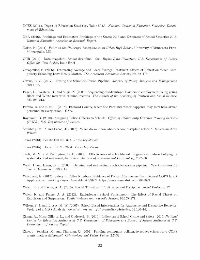
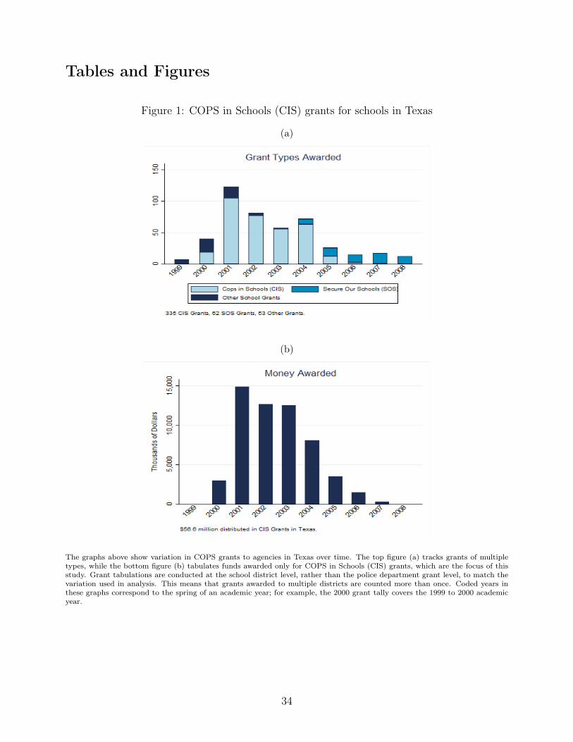
Figure 1 (a) shows that the majority of COPS school grants in Texas have been

distributed through the CIS program, with the objective of hiring of SROs in schools. Ap-

proximately seven percent of total federal CIS funds were distributed to Texas in this period.

The majority of grants were distributed between 2000 and 2004, with funding peaking at

≈ $15 million dollars in 2001.11 The bottom panel of Figure 1 shows that COPS grants for

school police have been consistently competitive, with grant applications outstripping grant

acceptances in each year of the program.

4 EMPIRICAL MODEL AND DATA SOURCES

The empirical model uses panel data to measure the impact of receiving a CIS grant within

school districts over time. I include school district fixed effects to account for unobserved

9These characterizations of school district police departments come from web searches of police depart-ments in Texas.

10Texas Appleseed included this information for a handful of districts in their 2010 report (Fowler et al.,2010). Data for Houston ISD and San Angelo ISD is from the 2006 to 2007 school year, while data forEdgewood ISD is from the 2007 to 2008 school year.

11Throughout this paper, years refer to the academic calendar indexed by the spring semester. For example,grant statistics for 2000 cover the 1999 to 2000 academic year.

11

differences across school districts that are constant over time. In addition, I control for the

non-random timing of school district decisions to apply for grants, which may be a function

of changes in disciplinary culture and student behavior within a district.

The empirical model is as follows:

Disciplineigdt = β1mAcceptdt ∗MiddleSchoolgt + β1hAcceptdt ∗HighSchoolgt+β2mApplydt ∗MiddleSchoolgt + β2hApplydt ∗HighSchoolgt+bmOtherGrantsdt + bhOtherGrantsdt

+πXigdt + δt + γg + φd + εigdt

LongtermOutcomeidt+k = α1AcceptExposuredt + α2ApplyExposuredt

+aOtherGrantsdt + π̃Xidt + δ̃t + φ̃d + νidt

where, i indexes students, g indexes grade, d indexes school district, and t indexes year.

Xigdt is a vector of covariates that includes district-grade enrollment and student race (Black,

Hispanic, White, or other race), gender, and whether the individual is classified as limited

English proficiency (LEP), Special Education, gifted and talented, or economically disadvan-

taged. δt are year fixed effects, which capture aggregate time trends in student outcomes

for all school districts. γg are grade-level fixed effects, which capture average differences in

disciplinary actions across grades.

The primary outcome in the analysis is whether a student received a disciplinary action

in a given year. This model uses student-year data for students in the 7th to 12th grade

between 1999 and 2008. In the long-term outcome model, I focus on student cohorts enrolled

in the 7th grade from 1999 to 2006 and measure high school graduation and college enrollment

within 8 years (by age 20). This approach allows me to measure high school graduation for a

broad base of 7th grade students and avoid issues of student attrition that may occur in later

grades. The student-level data was obtained through the Texas Education Research Center

12

(ERC), a research platform that combines databases on kindergarten through 12th grade

public-school students from the Texas Education Agency (TEA) and post-secondary students

in Texas higher education institutions from the Texas Higher Education Coordinating Board

(THECB).

The critical variables in the short-term model are Acceptdt and Applydt, which refer

to CIS grants. These variables are constructed to match the 3 year duration of CIS grant

projects. The variable Applydt is an indicator variable for whether a school district applied

for funding in year t, t−1, or t−2, allowing this variable to be set to 1 for the period in which

funding would be distributed if an application was accepted. Likewise, the variable Acceptdt

is an indicator for the duration of the grant project period if an application was accepted.12

For example, a school district police department that applies for and receives a CIS grant in

2000 would have Applydt and Acceptdt set to 1 during the period 2000 to 2002; while if the

grant application is denied, the Applydt variable would be set to 1 and the Acceptdt variable

would be set to 0 for this period.13 The variables OtherGrantsdt control for other school

grant programs administered from the COPS office, such as SOS grants. These controls are

comparably defined to the Acceptdt and Applydt variables.

The grant application and acceptance data used in this paper was obtained through

a Freedom of Information Act (FOIA) request to the COPS DOJ Office. I selected grants

based on whether the program type was focused on school police or if the applicant had their

12In practice, school districts do not directly apply for COPS funding. Grantees are commonly municipalpolice departments, independent school district police departments, or other entities. In some cases, grantapplications corresponded to a geographic area that covered more than one school district. In these instances,I manually matched grants to school districts using maps and web sources.

13The start time of a grant is indexed to the current academic year if a grant project (or application)starts between September and March, and is indexed to the following academic year if a project starts inApril through August. Throughout this project, academic years are denoted as the year of the spring semester.

13

primary jurisdiction within public schools (e.g. school district police departments).

I consider grant variables separately depending on whether the student is in middle

school (7th and 8th grade) or high school (9th through 12th grade), entering these variables

as interactions with grade type. I add this structure because in most districts students are

physically separated in different school buildings across these grades and SROs likely have

different capabilities and approaches to interacting with students in middle school and high

school. New SRO programs typically begin operating in high schools and then expand to

middle schools (and elementary schools) as they grow in size and scope. This pattern of

growth means that high schools are more likely to already have an SRO presence before

they receive a grant treatment. In addition to differences in treatment across middle and

high schools, students have developmental differences across these grades as well, which may

impact the way that they respond to increased SRO presence.

For the long-term outcome model, the estimation approach considers future outcomes

for cohorts of 7th graders. Here, the grant variables are defined in terms of years of exposure,

as the number of years within a grant application or acceptance period. Exposure is calculated

as a rate within the six years an "on-time" student would take to graduate high school between

the 7th and 12th grades. For example, consider a grant that is transferred to a school district

in the year 2000. A student beginning 7th grade in 2000 would be exposed to three accepted

grant years and have a value of 12for AcceptExposuredt and ApplyExposuredt. The exposure

values depend on the year that a student enters the 7th grade; in the above case, a student

in the 2001 7th grade cohort would be exposed to two years of a grant and have a calculated

exposure of 13between the 7th and 12th grades. OtherGrantsdt controls are also defined in

terms of exposure in the long-term model.

14

In this framework, Applydt illustrates changes in student outcomes when school dis-

tricts want to increase their police presence but do not receive grant funding. These variables

capture the effect of security initiatives a district could adopt on their own during years when

they are interested in federal funding for SROs. Acceptdt represents the impact of changes

in grant funding for school police conditional on the choice to apply for a grant. School

districts can alternate between grant acceptance states over time, switching between having

an accepted grant, a rejected grant, or no application.

The last important feature of the model are school district fixed effects, φd, which

control for unobserved differences across school districts that are constant over time.14 These

controls may reflect differences in district funding structures, approaches to discipline, and

cultures, each of which are determinants of student outcomes but are unobservable in the

data. After including school district fixed effects, the model uses variation across acceptance

years, rejected years, and years with no application within the same school district. The

specification is comparable to a difference-in-differences model with an additional control for

unobservable characteristics associated with the timing of application decisions (Appendix

Figure A1 depicts this comparison).15 The resulting identifying assumption is that conditional

on the decision to apply for a federal grant for school police, the timing of grant proposal

acceptance is not a function of changes in student outcomes within a school district.16

14Students are assigned to the school district they are enrolled in during the 7th grade, rendering theoutput of the model "intent-to-treat" estimates. This assignment procedure assumes that students do notalter their school district in response to school police presence prior to entering the 7th grade, an assumptionthat is reasonable given that levels of student discipline are low in kindergarten through 6th grades.

15All appendices referenced in the text are available at the end of this article as it appears inJPAM online. Go to the publisher’s website and use the search engine to locate the article athttp://www3.interscience.wiley.com/cgibin/jhome/34787

16While grant variables are defined as exposure rates in the long-term model, a similar identifying assump-tion holds because the timing of acceptances within districts determines the total number of years of grantexposure for school district cohorts.

15

The likelihood that a particular district wins a grant in one application year versus

another application year is a function of the availability of federal funds. The number of

possible grants that can be funded in each year varies with federal interest in the grant

programs, and this is a key driver of the probability that a grant application is accepted for

a particular district in a specific year (Figure 1, (c)).

A limitation of the model is that I am unable to observe the actual employment levels

of police in school districts. School districts do not directly employ police, instead they

are contracted through a third-party police department. Because I do not observe police

employment, the empirical approach does not use COPS grant variation as an instrument

for police presence; instead, I estimate the reduced form, or total, impact of receiving a CIS

grant on student outcomes.17 In the results section, I provide evidence that grants result in

increases in police presence by estimating impacts of the grants on school district security

spending. I also estimate increases in police hiring using a sub-sample of districts using data

from the Federal Bureau of Investigation (FBI).

A second concern is that grant funding may be used for other purposes, or affect other

aspects of a recipient’s spending that might also impact student outcomes. This project

focuses on CIS grants that are intended to be used to expand SRO hiring in public schools.

However, it is possible that some of the funds could be used for other security or other school

purposes, and this is a limitation of the study. This concern is mitigated by two factors. First,

the organizations that actually apply for COPS funding are third-party police departments,

and this organizational separation may make it more difficult for grant funds to be spent on

17Weisburst (2017) estimates a similar model using COPS grant acceptances as an instrument for policeemployment in municipal districts and to determine the impact of police force expansions on local crime rates.This two-stage model is possible because municipal police departments report employment to the FBI eachyear.

16

school initiatives that are not related to security. Second, while the focus of the model is

the effect of grants designated for police hiring, the specification also includes controls for

other school grants administered by the COPS office. The application controls for other grant

types partially account for interest in investing in alternate security aims, such as security

equipment and technology.

5 RESULTS

5.1 Summary Statistics

Table 1 provides a summary of the student data used in this project. The left panel describes

the short-term sample, covering over 16 million student-years between 1999 and 2008 for

students in the 7th through 12th grades. The right panel summarizes the long-term sample

of 2.5 million students in cohorts entering the 7th grade between 1999 and 2006.18 The

demographic characteristics across these two samples are similar.

The student sample is diverse; student observations are ≈ 40 percent White, 40 percent

Hispanic, 15 percent Black, and five percent other race, of which over 90 percent are Asian.

Half of the sample is categorized as economically disadvantaged, or low-income, a designation

that is derived from whether a student receives a free or reduced price lunch at school.19

26 percent of students receive disciplinary actions each year. Over the long term, 70

percent of 7th grade cohorts graduate from a public high school in Texas, and 47 percent

18The number of districts differs in the two samples due to district consolidation and reorganization in theperiod.

19This variable can also indicate low-income status using other definitions. These are annual income ator below the federal poverty line; eligibility for Aid to Families with Dependent Children or other publicassistance programs (includes WIC program participants); and eligibility for benefits under the Food StampAct of 1977 or the Health and Humans Services (HHS) Poverty Guidelines.

17

enroll in college within 8 years of enrolling in the 7th grade.

CIS grants affect a large portion of student-years in the data, with 42 percent of

observations corresponding to a grant application year and 25 percent of observations cor-

responding to a grant acceptance year (Table 1). These statistics imply a student-weighted

grant acceptance rate of 60 percent.

Over the time frame of the study, there were 771 CIS grant applications and 335

acceptances (Table 2).20 Awarded grants designated funding for three SROs per school district

on average, with total funds of $324,000 per school district (weighted by student-years). 80

percent of students attended school districts that applied for a grant during the sample

period, and 70 percent of students attended school districts that received a grant in the

sample period.21

5.2 Baseline Results

A necessary condition for interpreting the impact of CIS grants as a consequence of changes

to school security is that the grants significantly altered security resources. Table 3 measures

the relationship between CIS grants and security spending recorded by school districts, with

column (4) corresponding to the fully specified model. Panel (A) shows that the ratio of

security spending to total school district spending increases by approximately seven percent

when a school district has a CIS grant, from an average of 0.2 percent of total spending.22

20These counts are calculated to reflect counts of new grant-years by school districts. The summarystatistics in the table are weighted by student population, but the grant observations are at the school districtlevel.

21When grant characteristics are not weighted by student observations, 36 percent of districts applied fora grant during the sample period, 22 percent of districts were ever accepted for a grant, and 28 percent ofdistricts were ever rejected for a grant. These numbers are lower than the weighted characteristics becauselarger school districts were more likely to apply for and receive COPS funding.

22Throughout this paper, percentage effects are calculated relative to the outcome mean for the entiresample period, rather than a "pre-treatment" period because districts may be treated multiple times within

18

While not significant, Panel (B) shows that this corresponds to a point estimate increase of

$183,000 in security spending per year. This increase in spending is within range of one third

of the average three-year grant award of $324,000, suggesting that CIS grant funds were used

for school security rather than another purpose. While most districts regularly report having

some security expense, Panel (C) shows that school districts are one percent more likely to

report this expenditure when they are receiving a CIS grant, an outcome that could be related

to grant compliance.

These positive estimates show that school districts devote more resources to security

when covered by a federal grant. In practice, grants are typically administered to third-party

police departments rather than directly to schools and school district security budgets may

incompletely capture changes in grant spending. This institutional dynamic is likely to add

measurement error to the security spending outcome variables and may decrease precision in

these models.

Unfortunately, I cannot observe the impact of grant funding on SRO employment using

the Texas ERC data. However, I am able to examine police hiring impacts using data on a

sub-sample of Texas police departments from the FBI, in an analysis that is comparable to

Owens (2017). Appendix Table A1 shows that CIS grant acceptance results in up to a six

percent increase in the number of total police per 10,000 residents, and a 40 to 90 percent

increase in the number of SROs per 10,000 residents. While these estimates are derived from

small samples, they provide evidence that CIS grants are associated with increases in police

hiring.23

Table 4 shows the impact of grants for school police on student discipline. Panel (A)

the sample period.23For details on the estimation, refer to Appendix Table A1.

19

does not find a significant impact of grant funding on discipline when the effect is aggregated

across grades. However, grant receipt strongly increases disciplinary actions among middle

school students when the treatment is interacted with school type in Panel (B). Grant receipt

increases disciplinary actions among middle school students by six percent per year and does

not change rates of disciplinary actions for high school students. Table 5 shows that this in-

crease is driven by disciplinary actions for low-level offenses or conduct code violations, rather

than serious offenses. Appendix Table A2 provides evidence that out-of-school suspensions

are the most common sanction for these low level offenses.

The middle school discipline effect could be related to expansion of SROs from high

schools to middle schools with the assistance of grant funding. Though I cannot observe

how school districts allocate SROs across school types, the middle school treatment effect

is consistent with Owens (2017), who finds that CIS grants result in increases in arrests of

students 14 or younger on school grounds.

Students enrolled in schools with CIS grants also have lower high school graduation and

college enrollment rates. Police presence may create an adversarial school culture and alter

the experience of attending school. Likewise, additional disciplinary actions could stigmatize

disciplined students and reduce student confidence. Through these channels, school police

have the potential to reduce student attachment to school and student educational aspirations.

These channels could impact the likelihood of graduating high school or enrolling in college.24

24Throughout this project, I consider ultimate college enrollment outcomes for 7th grade cohorts that arenot conditional on high school graduation. I do this to estimate the primary policy relevant effect of changesin college enrollment for all students in attendance. This means that part of the college enrollment effect isdriven by students who do not complete high school and therefore cannot enroll in college. In fact, when thesample is restricted to students that ultimately graduate from high school, the percentage change in collegeenrollment is approximately half of the effect in the unconditional sample. These results are omitted due tospace constraints but are available on request.

20

Table 6 shows that the effect of exposure to one three-year CIS grant is associated

with a decline in the probability of graduating high school by 2.5 percent or 1.7 percentage

points.25 There is also a negative association between grant receipt and student college

enrollment rates, driven by a decline in two-year college enrollment. Exposure to one three

years CIS grant reduces the likelihood of ultimately enrolling in college by four percent and

the likelihood of enrolling in a four-year college by seven percent.

The estimates imply that a 10 percent increase in a school district’s security expense

ratio is associated with a 8.6 percent increase in middle school discipline per year, and 3.6

percent decline in high school graduation (for students exposed to a three year grant).

Each column in Tables 3, 4, 5 and 6 successively adds controls, with column (4) cor-

responding to the fully specified model. Adding student covariates to the model in columns

(2) and (4) does not substantively alter the estimates (across these tables). Adding appli-

cation controls to columns (3) and (4) in these tables accounts for time varying unobserved

characteristics associated with school district interest in grant funding. The application con-

trols are not always significant, but they do alter the "Accept" coefficient magnitude. These

coefficients imply that when districts choose to apply for funding they are less likely to have

a security budget and have higher high school graduation and college enrollment rates. The

preferred specification adjusts for changes in student outcomes that are associated with school

district decisions to apply for funding.

25The coefficient in the table corresponds to full grant exposure for six possible years between 7th and12th grade (or the equivalent of two grants). A single grant is two-year long and corresponds to half of theregression coefficient.

21

5.3 Robustness Tests of the Baseline Model

In this section, I conduct several robustness tests of the baseline model. First, I test the

validity of the identification assumption, that conditional on grant application decisions, the

timing of CIS grant acceptance is not a function of changes in student outcomes within a

school district. Figure 2 interacts the accept variables with year indicators before and after

treatment, to examine how treatment is related to changes in disciplinary outcomes over

time.26

These graphs show that the timing of CIS grant acceptance is unrelated to pre-

treatment changes in student disciplinary actions for middle school and high school students.

In the post-treatment years, disciplinary actions increase for middle school students but are

unchanged for high school students.

In contrast to the discipline outcome which varies by year, high school graduation

and college enrollment are cumulative outcomes that are observed only once per student. In

Figure 3, I consider how the impacts on long-term outcomes change with increased exposure to

grants. The figures show that students with more years of exposure to grants are increasingly

less likely to graduate from high school or enroll in college.

Next, I conduct a series of placebo tests that artificially vary the timing of treatment

to provide evidence that the results are not spurious. The purpose of this exercise is to

26Due to computational constraints, these graphs use data collapsed to the district-grade-year level thatis weighted by the number of students within these cells. The specification used for this event study isadapted from the primary model to accommodate the fact that districts may have multiple grant treatmentsat different points in time. These graphs are created by duplicating the data for each possible treatmentyear and stacking these data sets to form a "pseudo panel." For example, the 2003 sub-panel considers newapplications in 2003 and plots acceptance coefficients in the years prior to and following 2003, while alsoseparately controlling for potential concurrent treatments in years other than 2003 (such as a new grant in2001). In each year panel, the designated treatment year is considered over time, and treatments in adjacentyears are included as additional model controls.

22

benchmark the actual model result to regressions in which we do not expect to find a grant

treatment effect. In each test, I randomly assign "Accept" treatments to districts that have

applied for a grant in a given year, maintaining the overall acceptance rate for that year in

the sample. I replicate this procedure 1,000 times and plot the distribution of estimates in

Appendix Figure A2. The placebo distributions validate the actual estimates: The model

estimate for the impact of grant receipt is outside of the 95 percent confidence interval for

the increase in middle school discipline.

I extend this analysis to a test of the high school graduation and college enrollment

effects in Appendix Figure A3. Here, I randomize the fraction of years a student is exposed

to grant funding for each 7th grade district-cohort year such that this fraction is less than

the "Apply Exposure" fraction and the overall acceptance exposure matches the rate in the

data. Using this test, I find that the model estimates for high school graduation and college

enrollment are also outside the 95 percent confidence interval in the placebo distributions.

In Appendix Tables A3 and A4, I display a series of additional robustness checks. One

concern with the baseline model is that school districts that apply for or are accepted for

grants may be markedly different from districts that do not apply for grants. In the baseline

model, I include school district fixed effects to account for differences across these district

types that are constant over time. However, the time trends across districts with different

grant participation may differ. To test the importance of this concern, I first restrict the

sample to school districts that ever applied for a grant (specification 2), were ever accepted

for a grant (specification 3), or were both rejected and accepted for a grant (specification 4) to

allow the time trend and covariate coefficients to be estimated within group. In specification

(5), I include the full sample but interact year effects with four grant history groups, namely

23

those that never applied, were only accepted, were only rejected, or were both accepted and

rejected. Lastly in (6), I allow year effects to be separately estimated for districts that applied

for grants in different years. The estimates are comparable across each of these specifications.

A second concern is that school districts that are located in different parts of the state

or serve student populations of different sizes may have different trends in discipline and

long-term academic outcomes. I separately estimate year effects for 20 geographic regions in

Texas in specification (7), and 9 student enrollment size groups in specification (8). Again,

the estimates in these specifications are similar to the results of the baseline model.

School campuses within school districts may vary substantially in terms of student

characteristics, disciplinary policy, and other resources. In this paper, I focus on differences

in outcomes within school districts because I observe policy changes at the school district level.

In specification (9), I substitute school district fixed effects with school campus fixed effects

to address heterogeneity across schools within districts. This change does not substantively

alter the results.

A key component of this paper is considering how funding for police impacts students in

different race and income groups. Students in these different demographic groups likely have

different trends in discipline, high school graduation and college enrollment. Likewise, school

districts may have different approaches to discipline or have varying educational performance

across these student groups. In specifications (10) and (11), I explicitly allow the year fixed

effects and district fixed effects to vary by student race and income groups. Including these

additional controls does not alter the total coefficient on grant receipt. In the Treatment

Heterogeneity Section (Section 5.4) below, I utilize flexible models that allow year and district

fixed effects to vary by student race and income (comparable to specification 11).

24

A potential mechanism for the high school findings could be that students who are

most likely to be disciplined drop out of school when funding for police officers increases. I

test the importance of student attrition in explaining the findings by restricting the sample

to students who remain in school through the 10th grade or higher in specification (12). I

find consistent estimates for discipline in these samples, suggesting that student attrition is

a minor contributor to the findings.

In several of the analyses in this paper, I use data that is collapsed to the district-

level and weighted by student enrollment cells. As a sense check of this procedure, I include

estimates using collapsed data weighted by the number of students in each cell in (13).27

I include additional grade level robustness checks for the discipline outcome in Ap-

pendix Table A3. Specifications (14) and (15) show that the effects are robust to including

grade by year fixed effects and grade by district fixed effects. Lastly, the analysis in this

project is restricted to students in the 7th through 12th grade because students in this age

range have higher rates of discipline than younger students. I estimate the impact of CIS

grants for school police on students in the 1st through 6th grades in specification (16). I find

no effect of the grants on students in these grades, likely because both discipline rates and

police presence are low for these students.

5.4 Treatment Heterogeneity

In Tables 7 and 8, I consider treatment effects for different student demographic groups,

split by race and socioeconomic status, using the economic disadvantage indicator. I con-

27Proportional weights equal to hundreds of students are applied in the collapsed sample. The sample sizesin the weighted collapsed data set and the unweighted baseline differ due to rounding.

25

sider differences by race because of the large disciplinary gaps that have been documented

by researchers, policymakers, and advocates. Similarly, I consider student poverty because

poorer students also experience higher rates of discipline and are less likely to graduate from

high school.28 In each of the models in this section, I include flexible controls that allow time

trends and district fixed effects to vary by student race and income groups.29 Each model

interacts the main treatment effects with each student race and income group.

The demographic pattern of grant treatment effects on discipline is striking. Nearly

all groups of middle school students experience significant increases in discipline, but the

effects are strongest for low-income students and Black and Hispanic students. These effects

correspond to a five percent increase in discipline for low-income White students and an seven

percent increase in discipline for low-income Black and Hispanic students. For students that

are not low-income, Black students experience a ten percent increase in discipline, followed by

a six percent increase for Hispanic students and a four percent increase for White students.

The estimates imply that when school districts expand resources for school police, low-income

and minority students are disciplined more intensively.

The post-estimation tests at the bottom of Table 7 show that the treatment effects for

low-income students are not statistically different from one another across race. Further, the

treatment effects for both Black and Hispanic students are not statistically different from one

another across income groups (within race). As in the aggregated model, none of the groups

28I have also considered models that additionally interact the treatment effect with student gender. I donot find significant differences in treatment effects on discipline across gender and within race and incomegroups. In the long-term analysis there is some evidence that high school graduation effects are stronger formen and college enrollment effects are stronger for women. The results are omitted due to space constraintsbut available on request.

29These controls are not included in the baseline models above. The baseline models are robust to inclusionof these controls (see specifications 10 and 11 of Tables A3 and A4 above.

26

experiences significant changes in high school discipline.

The group mean column shows that there are also large baseline gaps in discipline by

race and socioeconomic class. Relative to White students that are not low-income, low-income

Black students are up to three times as likely to have a disciplinary action, while low-income

Hispanic and White students are two times as likely to have a disciplinary action. Likewise,

Black and Hispanic students that are not low-income are two times and one and a half times

more likely to have a disciplinary action.

Table 8 considers how treatment effects for high school graduation and college en-

rollment differ by student demographic group. The analysis shows significant decreases in

high school graduation for Hispanic and White students and significant decreases in college

enrollment for low-income Black, Hispanic and White students. However, I cannot reject

the null hypothesis that all treatment effects are equal for either outcome. These models do

not provide strong evidence that the declines in high school graduation or college enrollment

are concentrated in a particular student group. While somewhat less precise, the effects are

broadly consistent with estimated declines in middle school discipline that are experienced

by all student groups in Table 7. As in the discipline outcome, the group mean column in

this table shows that low-income students and minority students are less likely to graduate

high school (0.7 to 0.9 times) and enroll in college (0.5-0.9 times).

It is not surprising that funding for police in public schools differentially impacts stu-

dents with different demographic characteristics. Prior work has shown that school districts

with higher enrollment of non-White students are more likely to have "zero-tolerance" manda-

tory expulsion policies for certain offenses (Curran, 2017), that much of the racial disparity

in discipline exists across schools (Anderson and Ritter, 2017), and that school districts with

27

higher enrollment of Black students utilize more punitive discipline responses (Welch and

Payne, 2010, 2012). These studies are consistent with the findings in this project. The

observed patterns support a priori concerns that SROs disproportionately disadvantage low-

income students and Black and Hispanic students. Overall, the demographic analysis implies

that a student’s experience with school discipline at an early age has potential ramifications

for high school graduation and college enrollment. Negative school discipline experiences

could shape the way that students are perceived by teachers, school administrators, and

peers, and may also affect a student’s confidence and attachment to school.

6 CONCLUSION

The widespread use of police officers in public schools is a relatively recent development.

While school police programs have gained popularity as a policy to protect students against

rare but tragic school shooting events, in practice, these officers are often actively involved in

the enforcement of school discipline.

When school police officers are involved in the daily lives of students, they have the

capability to alter student behavior, disciplinary consequences, attachment to school, and

educational attainment. Though the potential consequences of school police interventions are

large, there have been few evaluations of their efficacy.

This study provides the first estimate of the impact of funding for school police on

student discipline and educational attainment using quasi-experimental methods. Using vari-

ation in federal COPS grants for school police, I measure the effect of receiving an increase in

funding on students, conditional on school district decisions to apply for this funding. This

28

strategy addresses biases related to both the non-random assignment of police to particular

school districts and the non-random timing of investments in police within school districts.

Using detailed data on over 2.5 million public-school students in the state of Texas,

I find that grants for school police increase disciplinary actions for middle school students.

Over the long-term, exposure to federal funding for school police is associated with small but

significant declines in high school graduation rates and college enrollment.

The results vary across student demographic groups. I find that expansions in grant

funding have the largest effects on low-income students and Black and Hispanic students.

This finding is consistent with prior work that finds that these marginalized student groups

are most vulnerable to school discipline sanctions. This disparate policy impact is concerning

and has implications for potential reforms to school policing and school discipline.

The large sample in the study, covering all students in public school in a populous and

diverse state, means the results are likely informative for other contexts. While the analysis

is limited by the fact that I cannot directly observe police employment in schools, the grant

transfers I examine approximate practical policies. Policymakers are often limited in their

capacity to monitor the implementation of regulations or subsidies; instead they are more

likely to administer funds for articulated goals, similar to the grant program that is the focus

of this study. This paper finds a negative average impact of grant transfers for school police

on student outcomes.

On the whole, the results suggest that SROs have the potential to negatively affect

students, through both increasing student discipline involvement and reducing student educa-

tional attainment. The literature on economic returns to schooling has shown that attending

an additional year of high school can raise individual earnings by approximately 10 percent

29

per year (Oreopoulos, 2006). Drawing on these findings, I conduct a back-of-the-envelope

calculation of costs of this policy. I consider only costs from the decline in high school grad-

uation and assume this decline results from only one less year of schooling for each student

that did not graduate. To be conservative, I assume baseline annual earnings of affected

students of $20,000 with a five percent earnings reduction per year, a discount rate of 20

percent, and a working career of 30 years.30 The resulting loss in earnings is $105 million

dollars for affected students, leading to an aggregate policy cost of $162 million including

the value of grant transfers. This calculation is illustrative: It does not include emotional or

psychological costs of school discipline, the value of increased safety or perceptions of safety,

benefits for subgroups of students who may be positively affected, costs of more than a sin-

gle year decrease in schooling, or costs related to reductions in college enrollment. Despite

these limitations, this exercise highlights the fact that the results in this study raise serious

questions about the value of future investments in school police.

More research is needed to understand how the utilization of public-school police com-

pares to alternative approaches to school discipline, including positive behavioral interventions

and supports and changes to disciplinary codes (Steinberg and Lacoe, 2017). Future work

should evaluate best practices in school discipline as well as the cost-effectiveness of different

disciplinary approaches.

30These values are purposefully conservative and likely provide an underestimate of costs. Median earningsfor individuals with less than a high school diploma ranged from $22,000 to $27,000 between 1995 and 2015,in 2015 dollars (NCES, 2016). Additionally, working careers often exceed 40 years, and discount rates areoften assumed to be less than 20 percent in net-present-value calculations. This calculation is based on thetreatment exposure rates in the sample, the estimated effect sizes for high school graduation. I estimate costsfrom students affected in the long-term sample, or the 8 cohorts of students enrolled in 7th grade from 1999to 2006.

30

ReferencesAddington, L. (2009). Cops and Cameras: Public School Security as a Policy Response to Columnbine.

American Behavioral Scientist, 52:1426–1446.

Aizer, A. and Doyle, J. (2015). Juvenile Incarceration, Human Capital, and Future Crime: Evidence fromRandomly Assigned Judges. The Quarterly Journal of Economics, 130:759–804.

Anderson, K. and Ritter, G. (2017). Disparate use of exclusionary discipline: Evidence on inequities in schooldiscipline from a u.s. state. Education Policy Analysis Archives, 25:1–36.

Balko, R. (2018). Putting more cops in schools won’t make schools safer, and it will likely inflict a lot ofharm. The Washington Post.

Bayer, P., Hjalmarsson, R., and Pozen, D. (2009). Building Criminal Capital behind Bars: Peer Effects inJuvenile Corrections. The Quarterly Journal of Economics, 124:105–147.

Brown, B. (2006). Understanding and assessing school police officers: A conceptual and methodologicalcomment. Journal of Criminal Justice, 34:591–604.

Brown, B. and Benedict, W. R. (2005). Classroom cops, what do the students think? A case study in studentperceptions of school police and security officers conducted in an Hispanic community. InternationalJournal of Police Science & Management, 7:264–285.

Camera, L. (2017). Civil Rights Spat Takes Center Stage in Education. U.S. News & World Report.

Canady, M., James, B., and Nease, J. (2012). To Protect and Educate: The School Resource Officer and thePrevention of Violence in Schools. National Association of School Resource Officers (NASRO).

Curran, C. (2016). Estimating the Effect of State Zero Tolerance Laws on Exclusionary Discipline, RacialDiscipline Gaps, and Student Behavior. Educational Evaluation and Policy Analysis, 20:1–22.

Curran, C. (2017). The Law, Policy, and Portrayal of Zero Tolerance School Discipline: Examining Prevalenceand Characteristics Across Levels of Governance and School Districts. Educational Policy, 32:1–39.

DeAngelo, G. and Hansen, B. (2014). Life and death in the fast lane: Police enforcement and traffic fatalities.American Economic Journal: Economic Policy, 6:231–257.

Devine, J. (1996). Maximum Security: The Culture of Violence in Inner-City Schools. The University ofChicago Press, Chicago, IL.

DeVoe, J., Peter, K., Kaufman, P., Ruddy, S., Miller, A., Planty, M., Snyder, T., and Rand, M. (2003).Indicators of School Crime and Safety: 2003. National Center for Education Statistics at U.S. Departmentof Education and Bureau of Justice Statistics at U.S. Department of Justice Report.

Di Tella, R. and Schargrodsky, E. (2004). Do police reduce crime? estimates using the allocation of policeforces after a terrorist attack. American Economic Review, 94:115–133.

DOJ (2018). Attorney General Sessions Announces New Actions To Improve School Safety And Better EnforceExisting Gun Laws. Office of Public Affairs at the Department of Justice.

Draca, M., Machin, S., and Witt, R. (2011). Panic on the streets of London: Police, crime, and the July 2005terror attacks. American Economic Review, 101:2157–2181.

EOP (2016). Report: The Continuing Need to Rethink Discipline. Executive Office of the President Report.

Evans, W. N. and Owens, E. G. (2007). COPS and crime. Journal of Public Economics, 91:181–201.

31

Fabelo, T., Thompson, M., Plotkin, M., Carmichael, D., Marchbanks, M., and Booth, E. (2011). BreakingSchools’ Rules: A Statewide Study of How School Discipline Relates to Students’ Success and JuvenileJustice Involvement. Justice Center at The Council of State Governments and Public Policy ResearchInstitute.

Finn, P. and McDevitt, J. (2005). National assessment of school resource officer programs. National Instituteof Justice Research Report.

Fisher, B. and Hennessy, E. (2016). School Resource Officers and Exclusionary Discipline in U.S. High Schools:A Systemic Review and Meta-analysis. Adolescent Research Review, 1:217–233.

Fowler, D. (2010). Fact Sheet: The Texas School-to-Prison Pipeline. Technical report, Texas Appleseed.

Fowler, D., Lightsey, R., Monger, J., and Aseltine, E. (2010). Texas’ School-to-Prison Pipeline: Ticketing,Arrest & Use of Force in Schools, How the Myth of the “Blackboard Jungle” Reshaped School DisciplinaryPolicy. Texas Appleseed Report.

GAO (2005). Community policing grants: COPS grants were a modest contributor to declines in crime inthe 1990s. Government Accountability Office, GAO-06-104.

Hanushek, E. A. and Welch, F., editors (2006). Handbook of the Economics of Education, volume 1. ElsevierScience and Technology, Amsterdam, Netherlands.

Hjalmarsson, R. (2008). Criminal justice involvement and high school completion. Journal of Urban Eco-nomics, 63:613–630.

James, N. and McCallion, G. (2013). School Resource Officers: Law Enforcement Officers in Public Schools.Congressional Research Service Report to Congress.

Kirk, D. and Sampson, R. (2011). Crime and the Production of Safe Schools. In Duncan, G. and Murnane,R., editors, Whither Opportunity? Rising Inequality, Schools, and Children’s Life Chances. Russell SageFoundation, New York, NY.

Klick, J. and Tabarrok, A. (2005). Using terror alert levels to estimate the effect of police on crime. Journalof Law and Economics, 48:267–279.

Kupchik, A. (2010). Homeroom Security: School Discipline in an Age of Fear. New York University Press,New York, NY.

Kupchik, A. and Ward, G. (2014). Race, Poverty, and Exclusionary School Security: An Empirical Analysisof U.S. Elementary, Middle, and High Schools. Youth Violence and Juvenile Justice, 12:332–354.

Lee, D. and McCrary, J. (2009). The deterrence effect of prison: Dynamic theory and evidence. PrincetonUniversity, Department of Economics, Working Paper 1168.

Lin, M.-J. (2009). More police, less crime: Evidence from U.S. state data. International Review of Law andEconomics, 29:73–80.

Lovenheim, M. and Owens, E. G. (2014). Does federal financial aid affect college enrollment? Evidence fromdrug offenders and the Higher Education Act of 1998. Journal of Urban Economics, 81:1–13.

Mendez, L. M. R. (2003). Predictors of suspension and negative school outcomes: A longitudinal investigation.New Directions for Youth Development, Fall:17–33.

Na, C. and Gottfredson, D. (2011). Police Officers in Schools: Effects on School Crime and the Processing ofOffending Behaviors. Justice Quarterly, pages 1–32.

Nagin, D. S. (2013). Deterrence in the Twenty-First Century. Crime and Justice, 42:199–263.

32

NCES (2016). Digest of Education Statistics, Table 502.3. National Center of Education Statistics, Depart-ment of Education.

NEA (2016). Rankings and Estimates: Rankings of the States 2015 and Estimates of School Statistics 2016.National Education Association Research Report.

Nolan, K. (2011). Police in the Hallways: Discipline in an Urban High School. University of Minnesota Press,Minneapolis, MN.

OCR (2014). Data snapshot: School discipline. Civil Rights Data Collection, U.S. Department of JusticeOffice for Civil Rights, Issue Brief 1.

Oreopoulos, P. (2006). Estimating Average and Local Average Treatment Effects of Education When Com-pulsory Schooling Laws Really Matter. The American Economic Review, 96:152–175.

Owens, E. G. (2017). Testing the School-to-Prison Pipeline. Journal of Policy Analysis and Management,36:11–37.

Pager, D., Western, B., and Sugie, N. (2009). Sequencing disadvantage: Barriers to employment facing youngBlack and White men with criminal records. The Annals of the Academy of Political and Social Science,623:195–213.

Perano, U. and Ellis, R. (2018). Broward County, where the Parkland attack happend, may soon have armedpersonnel in every school. CNN.

Raymond, B. (2010). Assigning Police Officers to Schools. Office of COmmunity Oriented Policing Services(COPS), U.S. Department of Justice.

Steinberg, M. P. and Lacoe, J. (2017). What do we know about school discipline reform? Education Next,Winter.

Texas (2013). Senate Bill No. 393. Texas Legislature.

Texas (2015). House Bill No. 2684. Texas Legislature.

Ttofi, M. M. and Farrington, D. P. (2011). Effectiveness of school-based programs to reduce bullying: asystematic and meta-analytic review. Journal of Experimental Criminology, 7:27–56.

Wald, J. and Losen, D. J. (2003). Defining and redirecting a school-to-prison pipeline. New Directions forYouth Development, 99:9–15.

Weisburst, E. (2017). Safety in Police Numbers: Evidence of Police Effectiveness from Federal COPS GrantApplications. Working Paper. Available at SSRN: https://ssrn.com/abstract=2845099.

Welch, K. and Payne, A. A. (2010). Racial Threat and Punitive School Discipline. Social Problems, 57.

Welch, K. and Payne, A. A. (2012). Exclusionary School Punishment: The Effect of Racial Threat onExpulsion and Suspension. Youth Violence and Juvenile Justice, 10:155–171.

Wilson, S. J. and Lipsey, M. W. (2007). School-Based Interventions for Aggressive and Disruptive Behavior:Update of a Meta-Analysis. American Journal of Preventative Medecine, 33:130–143.

Zhang, A., Musu-Gillette, L., and Oudekerk, B. (2016). Indicators of School Crime and Safety: 2015. NationalCenter for Education Statistics at U.S. Department of Education and Bureau of Justice Statistics at U.S.Department of Justice Report.

Zhao, J., Scheider, M., and Thurman, Q. (2002). Funding community policing to reduce crime: Have COPSgrants made a difference? Criminology and Public Policy, 2:7–32.

33

Tables and Figures

Figure 1: COPS in Schools (CIS) grants for schools in Texas

(a)

(b)

The graphs above show variation in COPS grants to agencies in Texas over time. The top figure (a) tracks grants of multipletypes, while the bottom figure (b) tabulates funds awarded only for COPS in Schools (CIS) grants, which are the focus of thisstudy. Grant tabulations are conducted at the school district level, rather than the police department grant level, to match thevariation used in analysis. This means that grants awarded to multiple districts are counted more than once. Coded years inthese graphs correspond to the spring of an academic year; for example, the 2000 grant tally covers the 1999 to 2000 academicyear.

34

Figure 1: CIS grants for schools in Texas

(c)

(d)

The graphs above show variation in COPS grants to agencies in Texas over time. The top figure (c) tracks new applications andacceptances of COPS in Schools (CIS) grants, while the bottom figure (d) tabulates duration years of an accepted CIS grant orintended CIS application. An "Acceptance-Year" refers to a year in the three year awarded grant period. An "Application-Year"refers to a year when either a grant was awarded or a grant would have been awarded, if rejected. Grant tabulations are conductedat the school district level, rather than the police department grant level, to match the variation used in analysis. This meansthat grants awarded to multiple districts are counted more than once. Coded years in these graphs correspond to the spring ofan academic year; for example, the 2000 grant tally covers the 1999 to 2000 academic year.

35

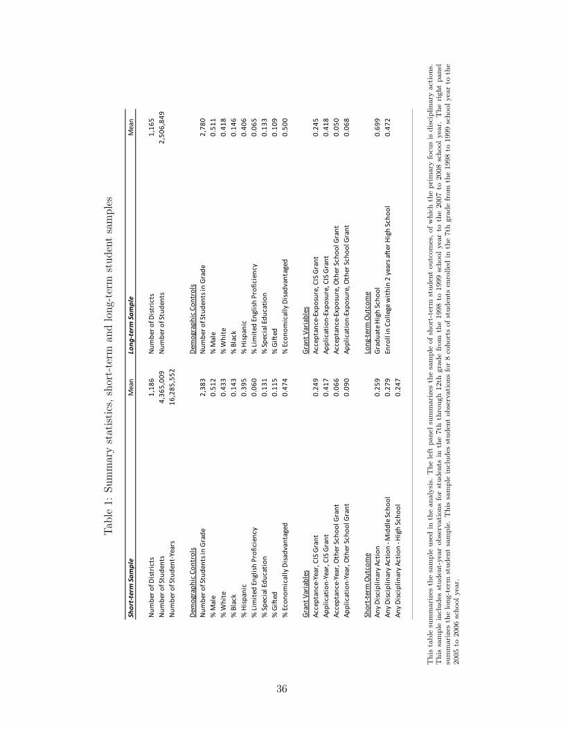
Table1:

Summarystatistics,s

hort-term

andlong

-term

stud

entsamples

Shor

t-ter

m Sa

mpl

eM

ea

nLo

ng-te

rm Sa

mpl

eM

ea

n

Nu

mb

er

of

Dis

tric

ts1

,18

6N

um

be

r o

f D

istr

icts

1,1

65

Nu

mb

er

of

Stu

de

nts

4,3

65

,00

9N

um

be

r o

f S

tud

en

ts2

,50

6,8

49

Nu

mb

er

of

Stu

de

nt-

Ye

ars

16

,28

5,5

52

De

mo

gra

ph

ic C

on

tro

lsD

em

og

rap

hic

Co

ntr

ols

Nu

mb

er

of

Stu

de

nts

in

Gra

de

2,3

83

Nu

mb

er

of

Stu

de

nts

in

Gra

de

2,7

80

% M

ale

0.5

12

% M

ale

0.5

11

% W

hit

e0

.43

3%

Wh

ite

0.4

18

% B

lac

k0

.14

3%

Bla

ck

0.1

46

% H

isp

an

ic0

.39

5%

His

pa

nic

0.4

06

% L

imit

ed

En

gli

sh P

rofi

cie

nc

y0

.06

0%

Lim

ite

d E

ng

lish

Pro

fic

ien

cy

0.0

65

% S

pe

cia

l E

du

ca

tio

n0

.13

1%

Sp

ec

ial

Ed

uc

ati

on

0.1

33

% G

ifte

d0

.11

5%

Gif

ted

0.1

09

% E

co

no

mic

all

y D

isa

dv

an

tag

ed

0.4

74

% E

co

no

mic

all

y D

isa

dv

an

tag

ed

0.5

00

Gra

nt

Va

ria

ble

sG

ran

t V

ari

ab

les

Ac

ce

pta

nc

e-Y

ea

r, C

IS G

ran

t0

.24

9A

cc

ep

tan

ce

-Ex

po

sure

, C

IS G

ran

t0

.24

5

Ap

pli

ca

tio

n-Y

ea

r, C

IS G

ran

t0

.41

7A

pp

lic

ati

on

-Ex

po

sure

, C

IS G

ran

t0

.41

8

Ac

ce

pta

nc

e-Y

ea

r, O

the

r S

ch

oo

l G

ran

t0

.06

6A

cc

ep

tan

ce

-Ex

po

sure

, O

the

r S

ch

oo

l G

ran

t0

.05

0

Ap

pli

ca

tio

n-Y

ea

r, O

the

r S

ch

oo

l G

ran

t0

.09

0A

pp

lic

ati

on

-Ex

po

sure

, O

the

r S

ch

oo

l G

ran

t0

.06

8

Sh

ort

-te

rm O

utc

om

eL

on

g-t

erm

Ou

tco

me

An

y D

isc

ipli

na

ry A

cti

on

0.2

59

Gra

du

ate

Hig

h S

ch

oo

l0

.69

9

An

y D

isc

ipli

na

ry A

cti

on

- M

idd

le S

ch

oo

l0

.27

9E

nro

ll i

n C

oll

eg

e w

ith

in 2

ye

ars

aft

er

Hig

h S

ch

oo

l0

.47

2

An

y D

isc

ipli

na

ry A

cti

on

- H

igh

Sc

ho

ol

0.2

47

Thistablesummarizes

thesampleused

inthean

alysis.The

left

panelsum

marizes

thesampleof

short-term

stud

entou

tcom

es,o

fwhich

theprim

aryfocusisdisciplin

aryaction

s.Thissampleinclud

esstud

ent-year

observations

forstud

ents

inthe7ththroug

h12th

grad

efrom

the1998

to1999

scho

olyear

tothe2007

to20

08scho

olyear.The

righ

tpa

nel

summarizes

thelong

-term

stud

entsample.

Thissampleinclud

esstud

entob

servations

for8coho

rtsof

stud

ents

enrolle

din

the7thgrad

efrom

the1998

to1999

scho

olyear

tothe

2005

to2006

scho

olyear.

36

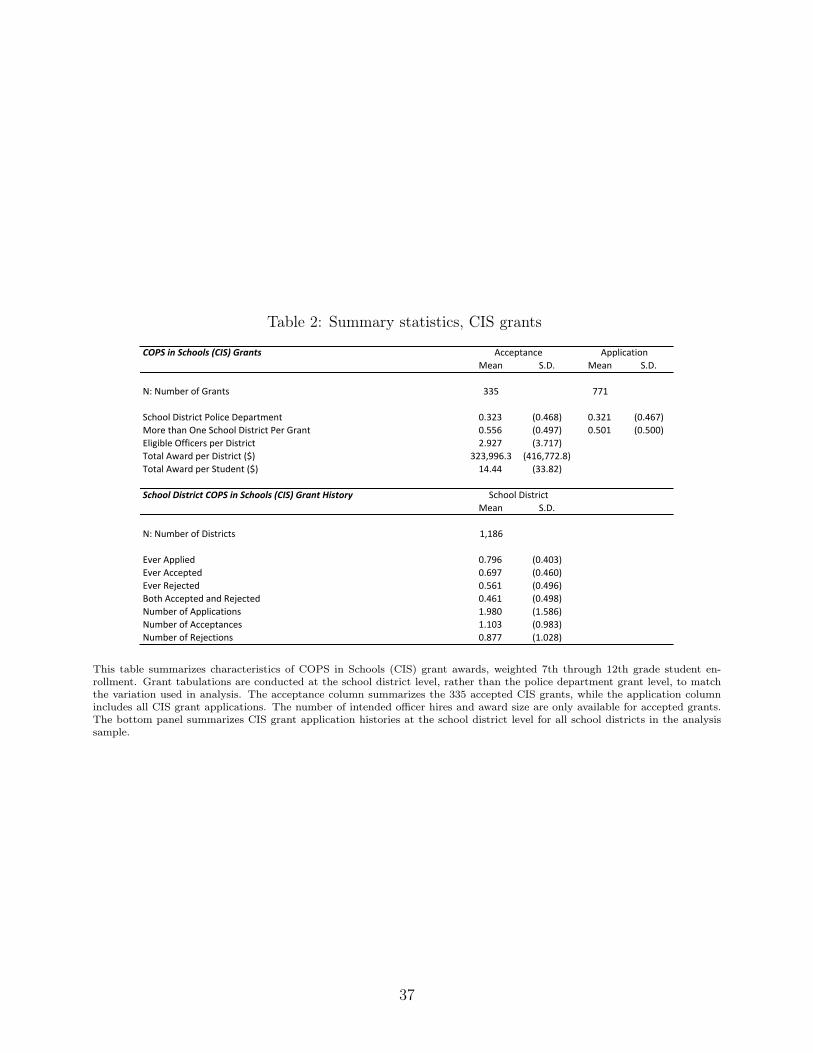
Table 2: Summary statistics, CIS grants

COPS%in%Schools%(CIS)%GrantsMean S.D. Mean S.D.

N:*Number*of*Grants 335 771

School*District*Police*Department 0.323 (0.468) 0.321 (0.467)More*than*One*School*District*Per*Grant 0.556 (0.497) 0.501 (0.500)Eligible*Officers*per*District 2.927 (3.717)Total*Award*per*District*($) 323,996.3 (416,772.8)Total*Award*per*Student*($) 14.44 (33.82)

School%District%COPS%in%Schools%(CIS)%Grant%HistoryMean S.D.

N:*Number*of*Districts 1,186

Ever*Applied 0.796 (0.403)Ever*Accepted 0.697 (0.460)Ever*Rejected* 0.561 (0.496)Both*Accepted*and*Rejected 0.461 (0.498)Number*of*Applications 1.980 (1.586)Number*of*Acceptances 1.103 (0.983)Number*of*Rejections 0.877 (1.028)

Acceptance Application

School*District

This table summarizes characteristics of COPS in Schools (CIS) grant awards, weighted 7th through 12th grade student en-rollment. Grant tabulations are conducted at the school district level, rather than the police department grant level, to matchthe variation used in analysis. The acceptance column summarizes the 335 accepted CIS grants, while the application columnincludes all CIS grant applications. The number of intended officer hires and award size are only available for accepted grants.The bottom panel summarizes CIS grant application histories at the school district level for all school districts in the analysissample.

37

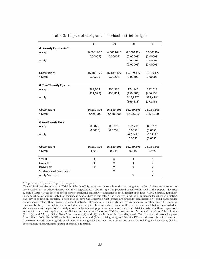
Table 3: Impact of CIS grants on school district budgets

(1) (2) (3) (4)A. Security Expense RatioAccept 0.000164* 0.000164* 0.000139+ 0.000139+

(0.00007) (0.00007) (0.00008) (0.00008)Apply 0.00003 0.00003

(0.00005) (0.00005)

Observations 16,189,127 16,189,127 16,189,127 16,189,127Y Mean 0.00206 0.00206 0.00206 0.00206

B. Total Security ExpenseAccept 389,938 393,960 174,141 182,617

(431,929) (430,811) (456,886) (456,938)Apply 346,837* 339,428*

(169,688) (172,756)

Observations 16,189,506 16,189,506 16,189,506 16,189,506Y Mean 2,428,000 2,428,000 2,428,000 2,428,000

C. Has Security FundAccept 0.0028 0.0026 0.0121* 0.0117*

(0.0035) (0.0034) (0.0052) (0.0051)Apply -0.0141* -0.0138*

(0.0055) (0.0055)

Observations 16,189,506 16,189,506 16,189,506 16,189,506Y Mean 0.945 0.945 0.945 0.945

Year FE X X X XGrade FE X X X XDistrict FE X X X XStudent-Level Covariates X XApply Controls X X

*** p<0.001, ** p<0.01, * p<0.05, + p<0.1This table shows the impact of COPS in Schools (CIS) grant awards on school district budget variables. Robust standard errorsare clustered at the school district level in all regressions. Column (4) is the preferred specification used in this paper. "SecurityExpense Ratio" is the ratio of school district spending on security functions to total district spending. "Total Security Expense"is the total dollar amount listed for security in school district budgets. "Has Security Fund" is an indicator for whether a districthad any spending on security. These models have the limitation that grants are typically administered to third-party policedepartments, rather than directly to school districts. Because of this institutional feature, changes in school security spendingmay not be fully recorded in the school district budget. Outcomes above vary at the district-year-level but are estimated instudent-year-level regressions to weight results by student population characteristics; the district clusters in these regressionsaccount for outcome duplication. Additional grant controls for other COPS school grants ("Accept Other Grant" in columns(1) to (4) and "Apply Other Grant" in columns (2) and (4)) are included but not displayed. Year FE are indicators for yearsfrom 1999 to 2008, Grade FE are indicators for grade-level (7th to 12th grade), and District FE are indicators for school district.Covariates include district grade enrollment, student gender and race, and student status as Limited English Proficiency (LEP),economically disadvantaged, gifted or special education.

38

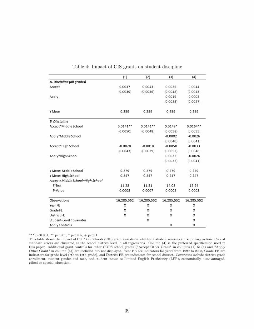
Table 4: Impact of CIS grants on student discipline

(1) (2) (3) (4)A. Discipline (all grades)Accept 0.0037 0.0043 0.0026 0.0044

(0.0039) (0.0036) (0.0048) (0.0043)Apply 0.0019 0.0002

(0.0028) (0.0027)

Y Mean 0.259 0.259 0.259 0.259

B. DisciplineAccept*Middle School 0.0141** 0.0141** 0.0148* 0.0164**

(0.0050) (0.0048) (0.0058) (0.0055)Apply*Middle School -0.0002 -0.0026

(0.0040) (0.0041)Accept*High School -0.0028 -0.0018 -0.0050 -0.0033

(0.0043) (0.0039) (0.0052) (0.0048)Apply*High School 0.0032 -0.0026

(0.0032) (0.0041)

Y Mean: Middle School 0.279 0.279 0.279 0.279Y Mean: High School 0.247 0.247 0.247 0.247Accept: Middle School=High School F-Test 11.28 11.51 14.05 12.94 P-Value 0.0008 0.0007 0.0002 0.0003

Observations 16,285,552 16,285,552 16,285,552 16,285,552Year FE X X X XGrade FE X X X XDistrict FE X X X XStudent-Level Covariates X XApply Controls X X

*** p<0.001, ** p<0.01, * p<0.05, + p<0.1This table shows the impact of COPS in Schools (CIS) grant awards on whether a student receives a disciplinary action. Robuststandard errors are clustered at the school district level in all regressions. Column (4) is the preferred specification used inthis paper. Additional grant controls for other COPS school grants ("Accept Other Grant" in columns (1) to (4) and "ApplyOther Grant" in column (4)) are included but not displayed. Year FE are indicators for years from 1999 to 2008, Grade FE areindicators for grade-level (7th to 12th grade), and District FE are indicators for school district. Covariates include district gradeenrollment, student gender and race, and student status as Limited English Proficiency (LEP), economically disadvantaged,gifted or special education.

39

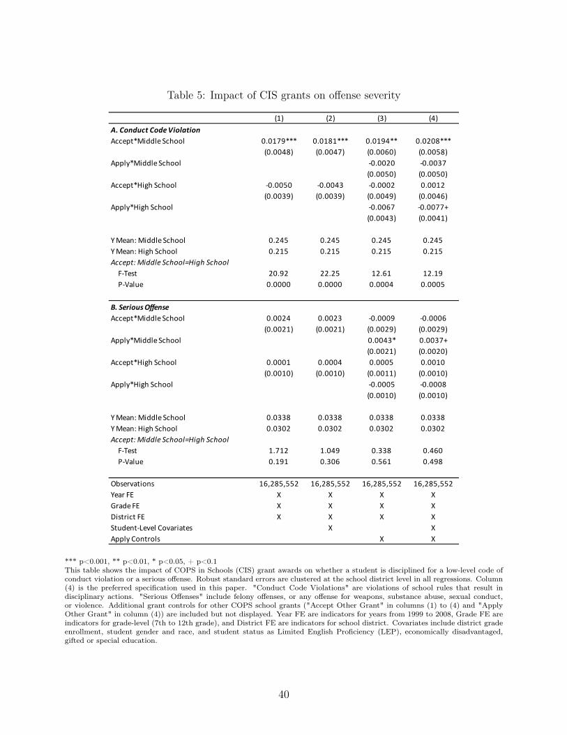
Table 5: Impact of CIS grants on offense severity

(1) (2) (3) (4)

A. Conduct Code ViolationAccept*Middle School 0.0179*** 0.0181*** 0.0194** 0.0208***

(0.0048) (0.0047) (0.0060) (0.0058)

Apply*Middle School -0.0020 -0.0037

(0.0050) (0.0050)

Accept*High School -0.0050 -0.0043 -0.0002 0.0012

(0.0039) (0.0039) (0.0049) (0.0046)

Apply*High School -0.0067 -0.0077+

(0.0043) (0.0041)

Y Mean: Middle School 0.245 0.245 0.245 0.245

Y Mean: High School 0.215 0.215 0.215 0.215

Accept: Middle School=High School F-Test 20.92 22.25 12.61 12.19

P-Value 0.0000 0.0000 0.0004 0.0005

B. Serious OffenseAccept*Middle School 0.0024 0.0023 -0.0009 -0.0006

(0.0021) (0.0021) (0.0029) (0.0029)

Apply*Middle School 0.0043* 0.0037+

(0.0021) (0.0020)

Accept*High School 0.0001 0.0004 0.0005 0.0010

(0.0010) (0.0010) (0.0011) (0.0010)

Apply*High School -0.0005 -0.0008

(0.0010) (0.0010)

Y Mean: Middle School 0.0338 0.0338 0.0338 0.0338

Y Mean: High School 0.0302 0.0302 0.0302 0.0302

Accept: Middle School=High School F-Test 1.712 1.049 0.338 0.460

P-Value 0.191 0.306 0.561 0.498

Observations 16,285,552 16,285,552 16,285,552 16,285,552

Year FE X X X X

Grade FE X X X X

District FE X X X X

Student-Level Covariates X X

Apply Controls X X

*** p<0.001, ** p<0.01, * p<0.05, + p<0.1This table shows the impact of COPS in Schools (CIS) grant awards on whether a student is disciplined for a low-level code ofconduct violation or a serious offense. Robust standard errors are clustered at the school district level in all regressions. Column(4) is the preferred specification used in this paper. "Conduct Code Violations" are violations of school rules that result indisciplinary actions. "Serious Offenses" include felony offenses, or any offense for weapons, substance abuse, sexual conduct,or violence. Additional grant controls for other COPS school grants ("Accept Other Grant" in columns (1) to (4) and "ApplyOther Grant" in column (4)) are included but not displayed. Year FE are indicators for years from 1999 to 2008, Grade FE areindicators for grade-level (7th to 12th grade), and District FE are indicators for school district. Covariates include district gradeenrollment, student gender and race, and student status as Limited English Proficiency (LEP), economically disadvantaged,gifted or special education.

40

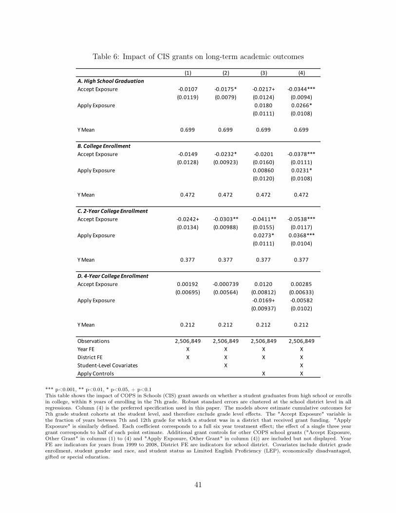
Table 6: Impact of CIS grants on long-term academic outcomes

(1) (2) (3) (4)A. High School GraduationAccept Exposure -0.0107 -0.0175* -0.0217+ -0.0344***

(0.0119) (0.0079) (0.0124) (0.0094)Apply Exposure 0.0180 0.0266*

(0.0111) (0.0108)

Y Mean 0.699 0.699 0.699 0.699

B. College EnrollmentAccept Exposure -0.0149 -0.0232* -0.0201 -0.0378***

(0.0128) (0.00923) (0.0160) (0.0111)Apply Exposure 0.00860 0.0231*

(0.0120) (0.0108)

Y Mean 0.472 0.472 0.472 0.472

C. 2-Year College EnrollmentAccept Exposure -0.0242+ -0.0303** -0.0411** -0.0538***

(0.0134) (0.00988) (0.0155) (0.0117)Apply Exposure 0.0273* 0.0368***

(0.0111) (0.0104)

Y Mean 0.377 0.377 0.377 0.377

D. 4-Year College EnrollmentAccept Exposure 0.00192 -0.000739 0.0120 0.00285

(0.00695) (0.00564) (0.00812) (0.00633)Apply Exposure -0.0169+ -0.00582

(0.00937) (0.0102)

Y Mean 0.212 0.212 0.212 0.212

Observations 2,506,849 2,506,849 2,506,849 2,506,849Year FE X X X XDistrict FE X X X XStudent-Level Covariates X XApply Controls X X

*** p<0.001, ** p<0.01, * p<0.05, + p<0.1This table shows the impact of COPS in Schools (CIS) grant awards on whether a student graduates from high school or enrollsin college, within 8 years of enrolling in the 7th grade. Robust standard errors are clustered at the school district level in allregressions. Column (4) is the preferred specification used in this paper. The models above estimate cumulative outcomes for7th grade student cohorts at the student level, and therefore exclude grade level effects. The "Accept Exposure" variable isthe fraction of years between 7th and 12th grade for which a student was in a district that received grant funding. "ApplyExposure" is similarly defined. Each coefficient corresponds to a full six year treatment effect; the effect of a single three yeargrant corresponds to half of each point estimate. Additional grant controls for other COPS school grants ("Accept Exposure,Other Grant" in columns (1) to (4) and "Apply Exposure, Other Grant" in column (4)) are included but not displayed. YearFE are indicators for years from 1999 to 2008, District FE are indicators for school district. Covariates include district gradeenrollment, student gender and race, and student status as Limited English Proficiency (LEP), economically disadvantaged,gifted or special education.

41

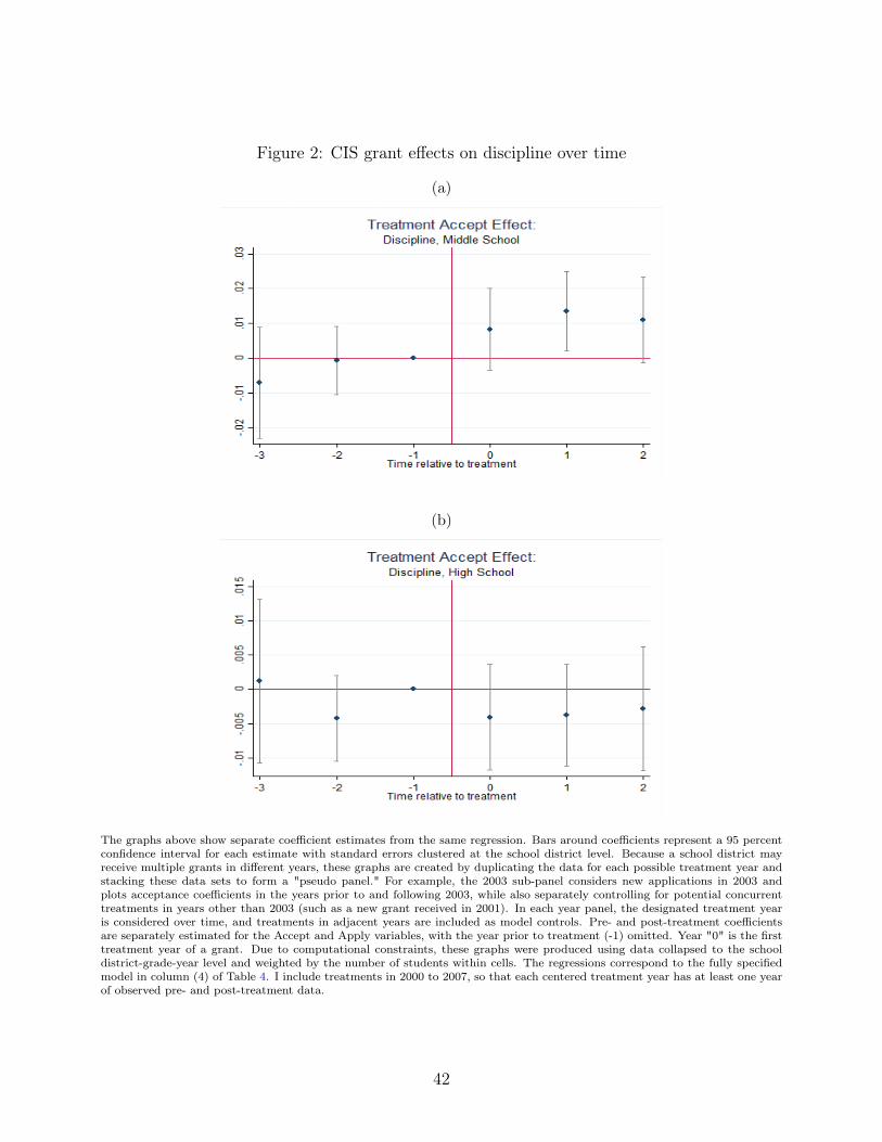
Figure 2: CIS grant effects on discipline over time

(a)

(b)

The graphs above show separate coefficient estimates from the same regression. Bars around coefficients represent a 95 percentconfidence interval for each estimate with standard errors clustered at the school district level. Because a school district mayreceive multiple grants in different years, these graphs are created by duplicating the data for each possible treatment year andstacking these data sets to form a "pseudo panel." For example, the 2003 sub-panel considers new applications in 2003 andplots acceptance coefficients in the years prior to and following 2003, while also separately controlling for potential concurrenttreatments in years other than 2003 (such as a new grant received in 2001). In each year panel, the designated treatment yearis considered over time, and treatments in adjacent years are included as model controls. Pre- and post-treatment coefficientsare separately estimated for the Accept and Apply variables, with the year prior to treatment (-1) omitted. Year "0" is the firsttreatment year of a grant. Due to computational constraints, these graphs were produced using data collapsed to the schooldistrict-grade-year level and weighted by the number of students within cells. The regressions correspond to the fully specifiedmodel in column (4) of Table 4. I include treatments in 2000 to 2007, so that each centered treatment year has at least one yearof observed pre- and post-treatment data.

42

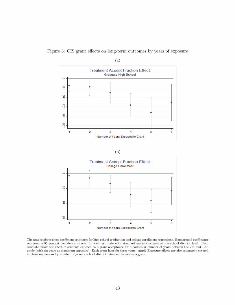
Figure 3: CIS grant effects on long-term outcomes by years of exposure

(a)

(b)

The graphs above show coefficient estimates for high school graduation and college enrollment regressions. Bars around coefficientsrepresent a 95 percent confidence interval for each estimate with standard errors clustered at the school district level. Eachestimate shows the effect of students exposed to a grant acceptance for a particular number of years between the 7th and 12thgrade (with six years as maximum exposure). Each grant lasts for three years. Apply Exposure effects are also separately enteredin these regressions by number of years a school district intended to receive a grant.

43

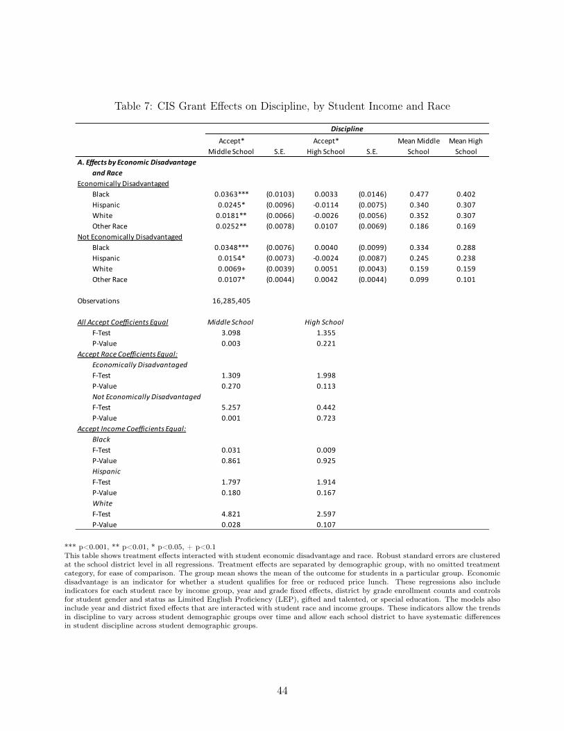
Table 7: CIS Grant Effects on Discipline, by Student Income and Race

Accept*Middle School S.E.

Accept*High School S.E.

Mean Middle School

Mean High School

A. Effects by Economic Disadvantageand Race

Economically DisadvantagedBlack 0.0363*** (0.0103) 0.0033 (0.0146) 0.477 0.402Hispanic 0.0245* (0.0096) -0.0114 (0.0075) 0.340 0.307White 0.0181** (0.0066) -0.0026 (0.0056) 0.352 0.307Other Race 0.0252** (0.0078) 0.0107 (0.0069) 0.186 0.169

Not Economically DisadvantagedBlack 0.0348*** (0.0076) 0.0040 (0.0099) 0.334 0.288Hispanic 0.0154* (0.0073) -0.0024 (0.0087) 0.245 0.238White 0.0069+ (0.0039) 0.0051 (0.0043) 0.159 0.159Other Race 0.0107* (0.0044) 0.0042 (0.0044) 0.099 0.101

Observations 16,285,405

All Accept Coefficients Equal Middle School High SchoolF-Test 3.098 1.355P-Value 0.003 0.221

Accept Race Coefficients Equal:Economically DisadvantagedF-Test 1.309 1.998P-Value 0.270 0.113Not Economically DisadvantagedF-Test 5.257 0.442P-Value 0.001 0.723

Accept Income Coefficients Equal:BlackF-Test 0.031 0.009P-Value 0.861 0.925HispanicF-Test 1.797 1.914P-Value 0.180 0.167WhiteF-Test 4.821 2.597P-Value 0.028 0.107

Discipline

*** p<0.001, ** p<0.01, * p<0.05, + p<0.1This table shows treatment effects interacted with student economic disadvantage and race. Robust standard errors are clusteredat the school district level in all regressions. Treatment effects are separated by demographic group, with no omitted treatmentcategory, for ease of comparison. The group mean shows the mean of the outcome for students in a particular group. Economicdisadvantage is an indicator for whether a student qualifies for free or reduced price lunch. These regressions also includeindicators for each student race by income group, year and grade fixed effects, district by grade enrollment counts and controlsfor student gender and status as Limited English Proficiency (LEP), gifted and talented, or special education. The models alsoinclude year and district fixed effects that are interacted with student race and income groups. These indicators allow the trendsin discipline to vary across student demographic groups over time and allow each school district to have systematic differencesin student discipline across student demographic groups.

44

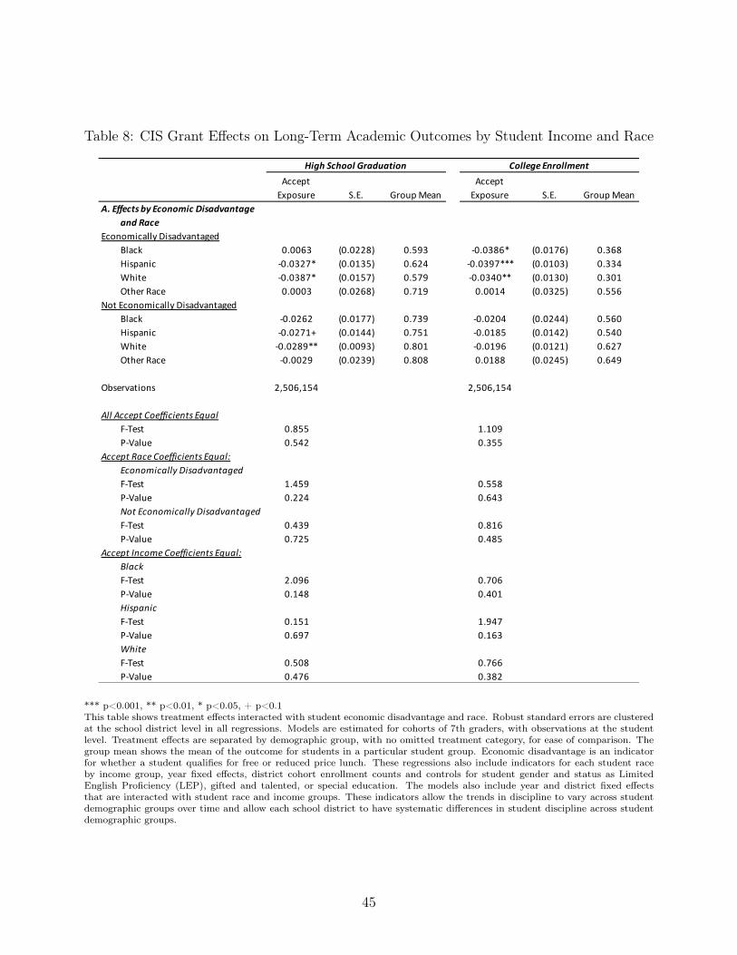
Table 8: CIS Grant Effects on Long-Term Academic Outcomes by Student Income and Race

Accept Exposure S.E. Group Mean

Accept Exposure S.E. Group Mean

A. Effects by Economic Disadvantageand Race

Economically DisadvantagedBlack 0.0063 (0.0228) 0.593 -0.0386* (0.0176) 0.368Hispanic -0.0327* (0.0135) 0.624 -0.0397*** (0.0103) 0.334White -0.0387* (0.0157) 0.579 -0.0340** (0.0130) 0.301Other Race 0.0003 (0.0268) 0.719 0.0014 (0.0325) 0.556

Not Economically DisadvantagedBlack -0.0262 (0.0177) 0.739 -0.0204 (0.0244) 0.560Hispanic -0.0271+ (0.0144) 0.751 -0.0185 (0.0142) 0.540White -0.0289** (0.0093) 0.801 -0.0196 (0.0121) 0.627Other Race -0.0029 (0.0239) 0.808 0.0188 (0.0245) 0.649

Observations 2,506,154 2,506,154

All Accept Coefficients EqualF-Test 0.855 1.109P-Value 0.542 0.355

Accept Race Coefficients Equal:Economically DisadvantagedF-Test 1.459 0.558P-Value 0.224 0.643Not Economically DisadvantagedF-Test 0.439 0.816P-Value 0.725 0.485

Accept Income Coefficients Equal:BlackF-Test 2.096 0.706P-Value 0.148 0.401HispanicF-Test 0.151 1.947P-Value 0.697 0.163WhiteF-Test 0.508 0.766P-Value 0.476 0.382

High School Graduation College Enrollment

*** p<0.001, ** p<0.01, * p<0.05, + p<0.1This table shows treatment effects interacted with student economic disadvantage and race. Robust standard errors are clusteredat the school district level in all regressions. Models are estimated for cohorts of 7th graders, with observations at the studentlevel. Treatment effects are separated by demographic group, with no omitted treatment category, for ease of comparison. Thegroup mean shows the mean of the outcome for students in a particular student group. Economic disadvantage is an indicatorfor whether a student qualifies for free or reduced price lunch. These regressions also include indicators for each student raceby income group, year fixed effects, district cohort enrollment counts and controls for student gender and status as LimitedEnglish Proficiency (LEP), gifted and talented, or special education. The models also include year and district fixed effectsthat are interacted with student race and income groups. These indicators allow the trends in discipline to vary across studentdemographic groups over time and allow each school district to have systematic differences in student discipline across studentdemographic groups.

45

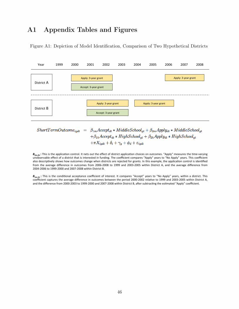
A1 Appendix Tables and Figures

Figure A1: Depiction of Model Identification, Comparison of Two Hypothetical Districts

District  A  

Year   1999   2002  2000   2001   2003   2004   2005   2006   2007   2008  

District  B  

Apply:  3-­‐year  grant  

Accept:  3-­‐year  grant  

Apply:  3-­‐year  grant  

Apply:  3-­‐year  grant  

Accept:  3-­‐year  grant  

Apply:  3-­‐year  grant  

Β2m,2h  :  This  is  the  applica@on  control.  It  nets  out  the  effect  of  district  applica@on  choices  on  outcomes.  “Apply”  measures  the  @me-­‐varying  unobservable  effect  of  a  district  that  is  interested  in  funding.  The  coefficient  compares  “Apply”  years  to  “No  Apply”  years.  This  coefficient  also  descrip@vely  shows  how  outcomes  change  when  districts  are  rejected  for  grants.  In  this  example,  the  applica@on  control  is  iden@fied  from   the   average   difference   in   outcomes   from   2006-­‐2008   to   1999   and   2003-­‐2005   within   District   A,   and   the   average   difference   from  2004-­‐2006  to  1999-­‐2000  and  2007-­‐2008  within  District  B.    Β1m,1h   :  This   is   the   condi@onal   acceptance   coefficient  of   interest.   It   compares   “Accept”   years   to   “No  Apply”   years,  within   a  district.   This  coefficient  captures  the  average  difference  in  outcomes  between  the  period  2000-­‐2002  rela@ve  to  1999  and  2003-­‐2005  within  District  A,  and  the  difference  from  2000-­‐2003  to  1999-­‐2000  and  2007-­‐2008  within  District  B,  aTer  subtrac@ng  the  es@mated  “Apply”  coefficient.        

46

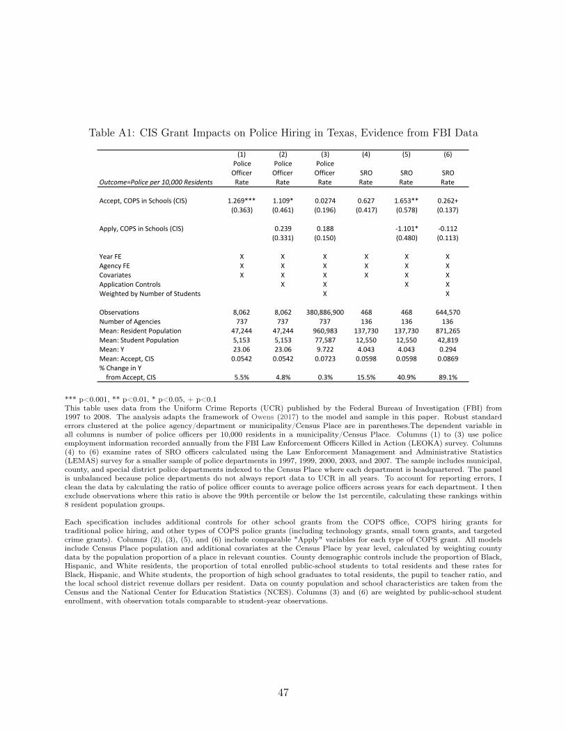
Table A1: CIS Grant Impacts on Police Hiring in Texas, Evidence from FBI Data

(1) (2) (3) (4) (5) (6)

Outcome=Police,per,10,000,Residents

Police/Officer/Rate

Police/Officer/Rate

Police/Officer/Rate

SRO/Rate

SRO/Rate

SRO/Rate

Accept,/COPS/in/Schools/(CIS) 1.269*** 1.109* 0.0274 0.627 1.653** 0.262+(0.363) (0.461) (0.196) (0.417) (0.578) (0.137)

Apply,/COPS/in/Schools/(CIS) 0.239 0.188 G1.101* G0.112(0.331) (0.150) (0.480) (0.113)

Year/FE X X X X X XAgency/FE X X X X X XCovariates X X X X X XApplication/Controls X X X XWeighted/by/Number/of/Students X X

Observations 8,062 8,062 380,886,900 468 468 644,570Number/of/Agencies 737 737 737 136 136 136Mean:/Resident/Population 47,244 47,244 960,983 137,730 137,730 871,265Mean:/Student/Population 5,153 5,153 77,587 12,550 12,550 42,819Mean:/Y 23.06 23.06 9.722 4.043 4.043 0.294Mean:/Accept,/CIS 0.0542 0.0542 0.0723 0.0598 0.0598 0.0869%/Change/in/Y/////from/Accept,/CIS 5.5% 4.8% 0.3% 15.5% 40.9% 89.1%

*** p<0.001, ** p<0.01, * p<0.05, + p<0.1This table uses data from the Uniform Crime Reports (UCR) published by the Federal Bureau of Investigation (FBI) from1997 to 2008. The analysis adapts the framework of Owens (2017) to the model and sample in this paper. Robust standarderrors clustered at the police agency/department or municipality/Census Place are in parentheses.The dependent variable inall columns is number of police officers per 10,000 residents in a municipality/Census Place. Columns (1) to (3) use policeemployment information recorded annually from the FBI Law Enforcement Officers Killed in Action (LEOKA) survey. Columns(4) to (6) examine rates of SRO officers calculated using the Law Enforcement Management and Administrative Statistics(LEMAS) survey for a smaller sample of police departments in 1997, 1999, 2000, 2003, and 2007. The sample includes municipal,county, and special district police departments indexed to the Census Place where each department is headquartered. The panelis unbalanced because police departments do not always report data to UCR in all years. To account for reporting errors, Iclean the data by calculating the ratio of police officer counts to average police officers across years for each department. I thenexclude observations where this ratio is above the 99th percentile or below the 1st percentile, calculating these rankings within8 resident population groups.

Each specification includes additional controls for other school grants from the COPS office, COPS hiring grants fortraditional police hiring, and other types of COPS police grants (including technology grants, small town grants, and targetedcrime grants). Columns (2), (3), (5), and (6) include comparable "Apply" variables for each type of COPS grant. All modelsinclude Census Place population and additional covariates at the Census Place by year level, calculated by weighting countydata by the population proportion of a place in relevant counties. County demographic controls include the proportion of Black,Hispanic, and White residents, the proportion of total enrolled public-school students to total residents and these rates forBlack, Hispanic, and White students, the proportion of high school graduates to total residents, the pupil to teacher ratio, andthe local school district revenue dollars per resident. Data on county population and school characteristics are taken from theCensus and the National Center for Education Statistics (NCES). Columns (3) and (6) are weighted by public-school studentenrollment, with observation totals comparable to student-year observations.

47

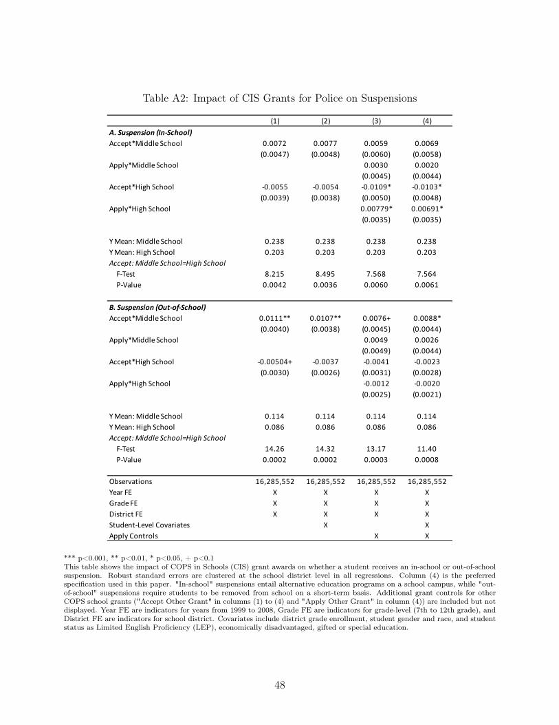
Table A2: Impact of CIS Grants for Police on Suspensions

(1) (2) (3) (4)

A. Suspension (In-School)Accept*Middle School 0.0072 0.0077 0.0059 0.0069

(0.0047) (0.0048) (0.0060) (0.0058)

Apply*Middle School 0.0030 0.0020

(0.0045) (0.0044)

Accept*High School -0.0055 -0.0054 -0.0109* -0.0103*

(0.0039) (0.0038) (0.0050) (0.0048)

Apply*High School 0.00779* 0.00691*

(0.0035) (0.0035)

Y Mean: Middle School 0.238 0.238 0.238 0.238

Y Mean: High School 0.203 0.203 0.203 0.203

Accept: Middle School=High School F-Test 8.215 8.495 7.568 7.564

P-Value 0.0042 0.0036 0.0060 0.0061

B. Suspension (Out-of-School)Accept*Middle School 0.0111** 0.0107** 0.0076+ 0.0088*

(0.0040) (0.0038) (0.0045) (0.0044)

Apply*Middle School 0.0049 0.0026

(0.0049) (0.0044)

Accept*High School -0.00504+ -0.0037 -0.0041 -0.0023

(0.0030) (0.0026) (0.0031) (0.0028)

Apply*High School -0.0012 -0.0020

(0.0025) (0.0021)

Y Mean: Middle School 0.114 0.114 0.114 0.114

Y Mean: High School 0.086 0.086 0.086 0.086

Accept: Middle School=High School F-Test 14.26 14.32 13.17 11.40

P-Value 0.0002 0.0002 0.0003 0.0008

Observations 16,285,552 16,285,552 16,285,552 16,285,552

Year FE X X X X

Grade FE X X X X

District FE X X X X

Student-Level Covariates X X

Apply Controls X X

*** p<0.001, ** p<0.01, * p<0.05, + p<0.1This table shows the impact of COPS in Schools (CIS) grant awards on whether a student receives an in-school or out-of-schoolsuspension. Robust standard errors are clustered at the school district level in all regressions. Column (4) is the preferredspecification used in this paper. "In-school" suspensions entail alternative education programs on a school campus, while "out-of-school" suspensions require students to be removed from school on a short-term basis. Additional grant controls for otherCOPS school grants ("Accept Other Grant" in columns (1) to (4) and "Apply Other Grant" in column (4)) are included but notdisplayed. Year FE are indicators for years from 1999 to 2008, Grade FE are indicators for grade-level (7th to 12th grade), andDistrict FE are indicators for school district. Covariates include district grade enrollment, student gender and race, and studentstatus as Limited English Proficiency (LEP), economically disadvantaged, gifted or special education.

48

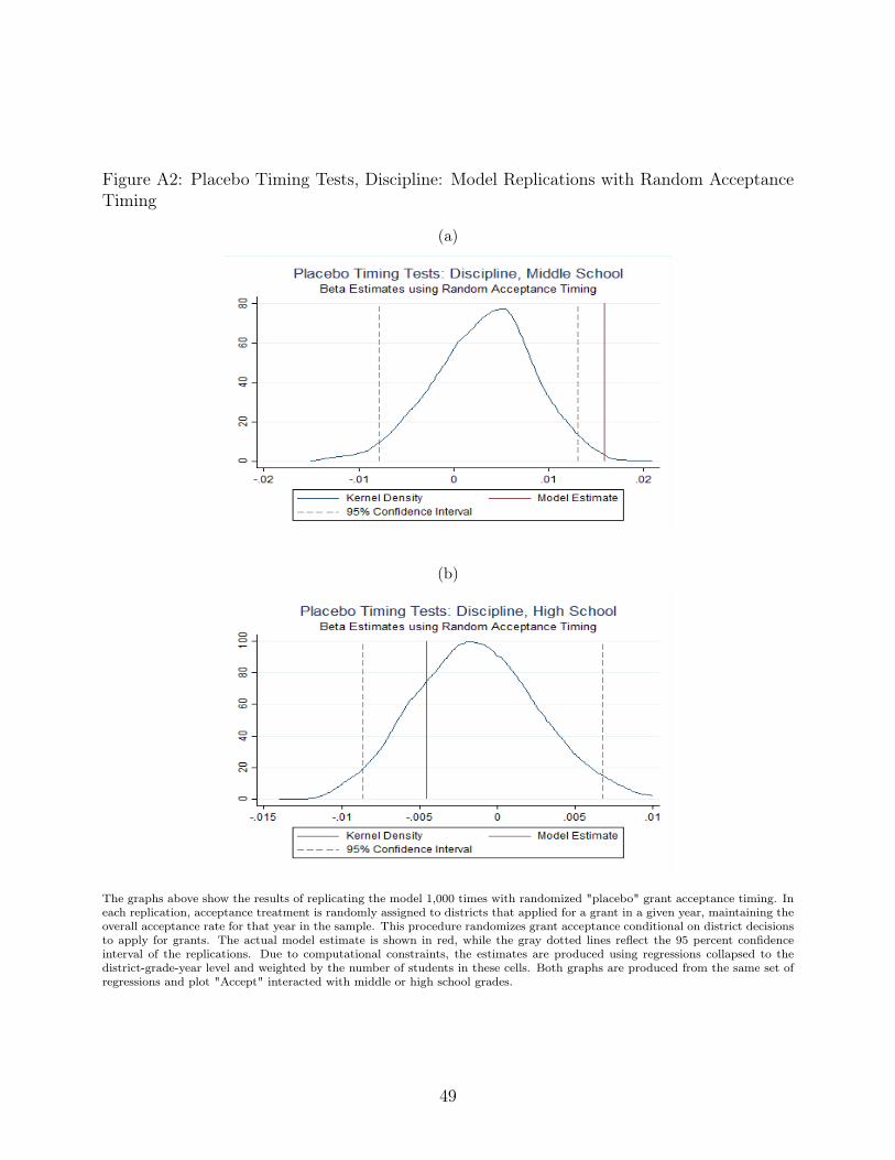
Figure A2: Placebo Timing Tests, Discipline: Model Replications with Random AcceptanceTiming

(a)

(b)

The graphs above show the results of replicating the model 1,000 times with randomized "placebo" grant acceptance timing. Ineach replication, acceptance treatment is randomly assigned to districts that applied for a grant in a given year, maintaining theoverall acceptance rate for that year in the sample. This procedure randomizes grant acceptance conditional on district decisionsto apply for grants. The actual model estimate is shown in red, while the gray dotted lines reflect the 95 percent confidenceinterval of the replications. Due to computational constraints, the estimates are produced using regressions collapsed to thedistrict-grade-year level and weighted by the number of students in these cells. Both graphs are produced from the same set ofregressions and plot "Accept" interacted with middle or high school grades.

49

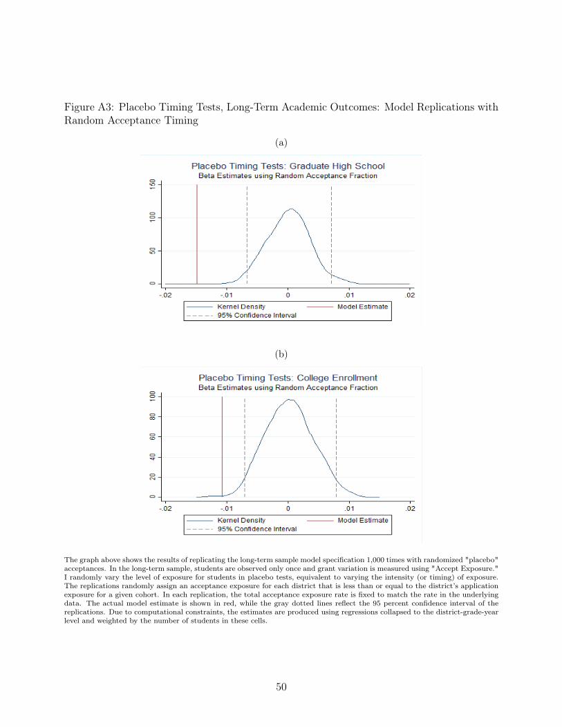
Figure A3: Placebo Timing Tests, Long-Term Academic Outcomes: Model Replications withRandom Acceptance Timing

(a)

(b)

The graph above shows the results of replicating the long-term sample model specification 1,000 times with randomized "placebo"acceptances. In the long-term sample, students are observed only once and grant variation is measured using "Accept Exposure."I randomly vary the level of exposure for students in placebo tests, equivalent to varying the intensity (or timing) of exposure.The replications randomly assign an acceptance exposure for each district that is less than or equal to the district’s applicationexposure for a given cohort. In each replication, the total acceptance exposure rate is fixed to match the rate in the underlyingdata. The actual model estimate is shown in red, while the gray dotted lines reflect the 95 percent confidence interval of thereplications. Due to computational constraints, the estimates are produced using regressions collapsed to the district-grade-yearlevel and weighted by the number of students in these cells.

50

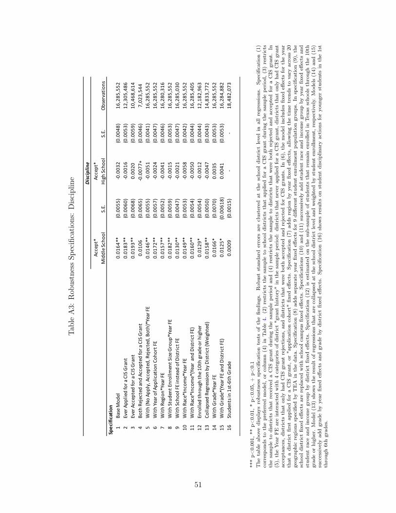
TableA3:

Rob

ustnessSp

ecification

s:Discipline

Acce

pt*

Mid

dle

Scho

olS.

E.Ac

cept

*H

igh

Scho

olS.

E.O

bser

vati

ons

Specificatio

n1

Base

Mod

el0.

0164

**(0

.005

5)-0

.003

2(0

.004

8)16

,285

,552

2Ev

er A

pplie

d fo

r a C

IS G

rant

0.01

83**

(0.0

060)

-0.0

016

(0.0

053)

12,3

05,4

863

Ever

Acc

epte

d fo

r a C

IS G

rant

0.01

93**

(0.0

068)

0.00

20(0

.005

9)10

,468

,614

4Bo

th R

ejec

ted

and

Acce

pted

for a

CIS

Gra

nt0.

0106

(0.0

065)

-0.0

077+

(0.0

046)

7,02

3,54

45

Wit

h (N

o Ap

ply,

Acc

epte

d, R

ejec

ted,

Bot

h)*Y

ear F

E0.

0146

**(0

.005

5)-0

.005

1(0

.004

1)16

,285

,552

6W

ith

Year

of A

pplic

atio

n Co

hort

FE

0.01

72**

(0.0

057)

-0.0

024

(0.0

047)

16,2

85,5

527

Wit

h Re

gion

*Yea

r FE

0.01

57**

(0.0

052)

-0.0

041

(0.0

046)

16,2

80,3

168

Wit

h St

uden

t Enr

ollm

ent S

ize

Gro

up*Y

ear F

E0.

0182

**(0

.005

9)-0

.001

5(0

.005

3)16

,285

,552

9W

ith

Scho

ol F

E in

stea

d of

Dis

tric

t FE

0.01

30**

(0.0

047)

-0.0

021

(0.0

047)

16,2

85,0

3010

Wit

h Ra

ce*I

ncom

e*Ye

ar F

E0.

0149

**(0

.005

3)-0

.005

8(0

.004

2)16

,285

,552

11W

ith

Race

*Inc

ome*

(Yea

r an

d D

istr

ict F

E)0.

0160

**(0

.005

4)-0

.005

0(0

.004

4)16

,285

,405

12En

rolle

d th

roug

h th

e 10

th g

rade

or h

ighe

r0.

0129

*(0

.005

4)-0

.001

2(0

.004

4)12

,182

,963

13Co

llaps

ed R

egre

ssio

n by

Dis

tric

t (W

eigh

ted)

0.01

58**

(0.0

050)

-0.0

047

(0.0

043)

14,8

33,7

7214

Wit

h G

rade

*Yea

r FE

0.01

66*

(0.0

070)

0.00

35(0

.005

3)16

,285

,552

15W

ith

Gra

de*(

Year

FE

and

Dis

tric

t FE)

0.01

25*

(0.0

0618

)0.

0041

(0.0

053)

16,2

84,8

8216

Stud

ents

in 1

st-6

th G

rade

0.00

09(0

.001

5)-

-18

,482

,073

Disciplin

e

***p<

0.001,

**p<

0.01,*p<

0.05,+

p<0.1

The

tableab

ovedisplays

robu

stness

specification

testsof

thefin

ding

s.Rob

uststan

dard

errors

areclusteredat

thescho

oldistrict

levelin

allregression

s.Sp

ecification

(1)

correspo

ndsto

thepreferredmod

el,or

column(4)in

Tab

le4.

(2)restrictsthesampleto

scho

oldistrictsthat

appliedforaCIS

gran

tdu

ring

thesamplepe

riod

,(3)restricts

thesampleto

districtsthat

received

aCIS

gran

tdu

ring

thesamplepe

riod

and(4)restrictsthesampleto

districtsthat

werebo

threjected

andaccepted

foraCIS

gran

t.In

(5),

theYearFE

areinteracted

with4catego

ries

ofdistrict

"grant

history"

inthesamplepe

riod

:districtsthat

neverap

pliedforaCIS

gran

t,districtsthat

only

hadCIS

gran

tacceptan

ces,

districtsthat

only

hadCIS

gran

trejections,an

ddistrictsthat

werebo

thaccepted

andrejected

forCIS

gran

ts.In

(6),

themod

elinclud

esfix

edeff

ects

fortheyear

that

adistrict

first

appliedforaCIS

gran

t,or

"app

licationcoho

rt"fix

edeff

ects.Sp

ecification

(7)ad

dsregion

byyear

fixed

effects,allowingthetimetrends

tovary

across

20geograph

icregion

sspecified

byTEA

intheda

ta.Sp

ecification

(8)ad

dssepa

rate

year

fixed

effects

for9diffe

rent

stud

enten

rollm

entpo

pulation

grou

ps.In

specification

(9),

the

scho

oldistrict

fixed

effects

arereplaced

withscho

olcampu

sfix

edeff

ects.Sp

ecification

s(10)

and(11)

successively

addstud

entrace

andincomegrou

pby

year

fixed

effects

and

stud

entrace

andincomegrou

pby

district

fixed

effects.Sp

ecification

(12)

isestimated

onthesub-sampleof

stud

ents

that

remainenrolle

din

Texas

scho

olsthroug

hthe10th

grad

eor

high

er.Mod

el(13)

show

stheresultof

regression

sthat

arecolla

psed

atthescho

oldistrict

levelan

dweigh

tedby

stud

entenrollm

ent,respectively.Mod

els(14)

and(15)

successively

addgrad

eby

year

fixed

effects

andgrad

eby

district

fixed

effects.Sp

ecification

(16)

show

sresultson

stud

entdisciplin

aryaction

sforyoun

gerstud

ents

inthe1st

throug

h6thgrad

es.

51

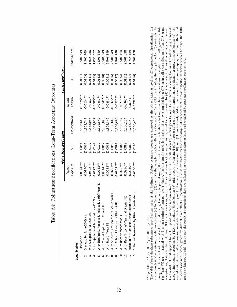
TableA4:

Rob

ustnessSp

ecification

s:Lo

ng-Term

Academic

Outcomes

Acce

pt

Expo

sure

S.E.

Obse

rvat

ions

Acce

pt

Expo

sure

S.E.

Obse

rvat

ions

Specificatio

n1

Base

Mod

el-0

.034

4***

(0.0

094)

2,50

6,84

9-0

.037

8***

(0.0

111)

2,50

6,84

92

Ever

App

lied

for a

CIS

Gra

nt-0

.027

6**

(0.0

097)

1,90

2,74

9-0

.029

4**

(0.0

109)

1,90

2,74

93

Ever

Acc

epte

d fo

r a C

IS G

rant

-0.0

392*

**(0

.011

7)1,

625,

058

-0.0

387*

*(0

.013

1)1,

625,

058

4Bo

th R

ejec

ted

and

Acce

pted

for a

CIS

Gra

nt-0

.067

2***

(0.0

147)

1,09

1,09

7-0

.058

0***

(0.0

155)

1,09

1,09

75

With

(No

Appl

y, A

ccep

ted,

Rej

ecte

d, B

oth)

*Yea

r FE

-0.0

382*

*(0

.013

2)2,

506,

849

-0.0

381*

*(0

.013

2)2,

506,

849

6W

ith Ye

ar o

f App

licat

ion

Coho

rt FE

-0.0

344*

**(0

.009

2)2,

506,

849

-0.0

341*

**(0

.009

8)2,

506,

849

7W

ith R

egio

n*Ye

ar FE

-0.0

282*

*(0

.008

8)2,

506,

849

-0.0

251*

*(0

.008

1)2,

506,

849

8W

ith St

uden

t Enr

ollm

ent S

ize G

roup

*Yea

r FE

-0.0

253*

*(0

.009

6)2,

506,

849

-0.0

365*

**(0

.010

6)2,

506,

849

9W

ith Sc

hool

FE in

stea

d of

Dist

rict F

E-0

.034

8***

(0.0

096)

2,50

6,63

0-0

.028

2**

(0.0

087)

2,50

6,84

910

With

Rac

e*In

com

e*Ye

ar FE

-0.0

252*

*(0

.008

8)2,

506,

154

-0.0

275*

*(0

.008

4)2,

506,

154

11W

ith R

ace*

Inco

me*

(Yea

r an

d Di

stric

t FE)

-0.0

256*

*(0

.008

9)2,

506,

154

-0.0

362*

*(0

.011

1)2,

506,

630

12En

rolle

d th

roug

h th

e 10t

h gr

ade o

r hig

her

-0.0

239*

*(0

.008

9)1,

755,

159

-0.0

185+

(0.0

112)

1,75

5,15

913

Colla

psed

Reg

ress

ion

by D

istric

t (W

eigh

ted)

-0.0

356*

**(0

.010

0)2,

506,

498

-0.0

392*

**(0

.011

6)2,

506,

498

High

Scho

ol G

radu

atio

nCo

llege

Enro

llmen

t

***p<

0.001,

**p<

0.01,*p<

0.05,+

p<0.1

The

tableab

ovedisplays

robu

stness

specification

testsof

thefin

ding

s.Rob

uststan

dard

errors

areclusteredat

thescho

oldistrict

levelin

allregression

s.Sp

ecification

(1)

correspo

ndsto

thepreferredmod

el,or

column(4)in

Tab

le4.

(2)restrictsthesampleto

scho

oldistrictsthat

appliedforaCIS

gran

tdu

ring

thesamplepe

riod

,(3)restrictsthe

sampleto

districtsthat

received

aCIS

gran

tdu

ring

thesamplepe

riod

and(4)restrictsthesampleto

districtsthat

werebo

threjected

andaccepted

foraCIS

gran

t.In

(5),

theYearFE

areinteracted

withfour

categories

ofdistrict

"grant

history"

inthesamplepe

riod

:districtsthat

neverap

pliedforaCIS

gran

t,districtsthat

only

hadCIS

gran

tacceptan

ces,

districtsthat

only

hadCIS

gran

trejections,an

ddistrictsthat

werebo

thaccepted

andrejected

forCIS

gran

ts.In

(6),

themod

elinclud

esfix

edeff

ects

fortheyear

that

adistrict

first

appliedforaCIS

gran

t,or

"app

licationcoho

rt"fix

edeff

ects.Sp

ecification

(7)ad

dsregion

byyear

fixed

effects,allowingthetimetrends

tovary

across

20geograph

icregion

sspecified

byTEA

intheda

ta.Sp

ecification

(8)ad

dssepa

rate

year

fixed

effects

for9diffe

rent

stud

enten

rollm

entpo

pulation

grou

ps.In

specification

(9),

the

scho

oldistrict

fixed

effects

arereplaced

withscho

olcampu

sfix

edeff

ects.Sp

ecification

s(10)

and(11)

successively

addstud

entrace

andincomegrou

pby

year

fixed

effects

and

stud

entrace

andincomegrou

pby

district

fixed

effects.Sp

ecification

(12)

isestimated

onthesub-sampleof

stud

ents

that

remainenrolle

din

Texas

scho

olsthroug

hthe10th

grad

eor

high

er.Mod

el(13)

show

stheresultof

regression

sthat

arecolla

psed

atthescho

oldistrict

levelan

dweigh

tedby

stud

entenrollm

ent,respectively.

52