Conformal Gravity

Patric Hölscher

Faculty of Physics, Bielefeld Universitypatric.hoelscher@physik.uni-bielefeld.de

Master Thesis in Theoretical Physics

September 2015

Supervisor and Referee: Prof. Dr. Dominik SchwarzSecond Supervisor: Dr. Daniel Boriero

Statutory DeclarationI declare that I have authored this thesis independently, that I have not usedother than the declared sources/resources, and that I have explicitly markedall material which has been quoted either literally or by content from the usedsources.

Contents1 Motivation 1

2 Introduction to Conformal Weyl Gravity 32.1 General Relativity . . . . . . . . . . . . . . . . . . . . . . . . . 32.2 Modifications of General Relativity . . . . . . . . . . . . . . . . 5

3 The Dark Matter Problem 93.1 Derivation and Solution of the Bach Equations . . . . . . . . . . 93.2 Newtonian Limit . . . . . . . . . . . . . . . . . . . . . . . . . . 12

3.2.1 Problem with Cavendish-type experiments . . . . . . . . 133.2.2 Circumvention of the Cavendish-type Problem . . . . . . 15

3.3 Galaxy Rotation Curves . . . . . . . . . . . . . . . . . . . . . . 173.3.1 Universality in the Data . . . . . . . . . . . . . . . . . . 213.3.2 Fit with a Linear Potential Term . . . . . . . . . . . . . 22

4 Quantization 27

5 Mass Generation 325.1 The Energy-Momentum Tensor of Test Particles and Perfect

Fluids . . . . . . . . . . . . . . . . . . . . . . . . . . . . . . . . 325.2 Dynamical Mass Generation . . . . . . . . . . . . . . . . . . . . 335.3 Comparison with a Kinematic Fermion Mass Theory . . . . . . 37

6 Cosmology in Conformal Gravity 396.1 The wrong Sign of the linear Potential Term . . . . . . . . . . . 43

7 Wave Equation and its Solution 447.1 Linearization of the Bach Equation . . . . . . . . . . . . . . . . 457.2 Inhomogeneous Wave Equation . . . . . . . . . . . . . . . . . . 46

8 Summary and Outlook 51

A Appendix 56

1 MotivationDespite the great success of General Relativity in describing the physics ofthe Solar System and the dynamics of the Universe in total, there are stillsome puzzles left. When Albert Einstein introduced his theory of GeneralRelativity in 1915 there were no measurements, which tested gravity on scalesfar beyond the distances of the Solar System. Therefore, as General Relativitywas able to solve several problems like the gravitational bending of light or theprecession of the perihelion of Mercury, it was quite natural to accept it as thestandard theory for gravity. But nowadays there is data from far more distantobjects, like other galaxies or galaxy clusters. On these distance scales therearise several problems. For example the measurement of rotational velocitiesof stars or gas in galaxies differs very strongly from the expectation. Thus, itis only possible to fit this behavior by invoking some unknown Dark Matter,which interacts with the baryonic matter only via gravity or via the weak force,but not electromagnetically or strongly.

Another issue is the cosmological constant problem. Since the measure-ments of Edwin Hubble in 1929 we know that the Universe is not static as itwas first assumed by Einstein, but as we know today it expands accelerated.Since all types of matter known so far are attracting each other via gravity,there has to be some kind of matter or energy that pushes matter apart. Thissubstance is called Dark Energy and its nature is unknown today, too. Itwould be appealing to identify this unknown Dark Energy with the zero-pointenergy of the matter fields of the Standard Model. But the calculated zero-point energy density of the Standard Model and the measured value, differ by120 orders of magnitude. One could solve this problem simply by fine-tuningthe comological constant, but this seems to be ridiculously unlikely.

Strongly coupled to this is the problem of combining gravity and quantummechanics at high energies. This means that treating the gravitational field asa quantum field exposes that General Relativity is non-powercounting renor-malizable. Therefore, it is not a reliable theory in the regime of high energies.

Hence, it is quite reasonable to ask whether instead of unknown matter orenergy that cures all the problems of General Relativity, it is the theory ofgravity itself, which has to be modified in such a way that there are modi-fications on big distance scales, but the behavior on Solar System scales iskept.

There are several approaches to modify gravity, like gravitational scalarfields, extra spatial dimensions, higher-order derivatives in the action or non-Christoffel connections, but non of them totally convincing.

In this thesis, we want to investigate an approach by Philip D. Mannheim[1, 2, 3], which belongs to the category of higher-order derivatives in the action.It is called “Conformal (Weyl) Gravity”. This theory is able to tackle thementioned problems of Dark Matter, Dark Energy and quantum gravity andthus it is worth investigating this theory in more detail.

We start with a presentation of the general idea of this theory in chapter2. In chapter 3 we deal with the Dark Matter problem and its solution in

1

Conformal Gravity. After that in chapter 4 we have a brief look at the quant-ization mechanism of the theory and how it deals with the zero-point energyproblem. In chapter 5, it is investigated, how the matter particles acquire massvia a dynamical Higgs mechanism. This mass generation mechanism is used inchapter 6 to study conformal cosmology. In chapter 7 we present an approachto study classical gravitational waves of gravitational bounded systems likebinary systems of stars and black holes in Conformal Gravity. The first stepsof solving the fourth-order wave equation are shown. The next step will bethe calculation of the radiated power for such a system. But this is still workin progress. In the end we give an outlook of open problems and further workthat has to be done.

2

2 Introduction to Conformal Weyl GravityThis chapter is an introduction to the theory of Conformal Gravity. We startwith the general formalism of General Relativity and introduce importantquantities and conventions. After that we investigate, what changes in theformalism of Conformal Gravity and address some general problems and diffi-culties that may be solved within Conformal Gravity. This introduction followsmainly two publications by Mannheim et. al. [1, 2].

2.1 General RelativityLet us first investigate which properties of GR make it so successful to describethe Solar System phenomenology. We know that Einstein wanted to generalizehis theory of Special Relativity to a theory that does not only work for constantmoving observers, but which is also compatible with accelerated observers.Furthermore, it was necessary to bring Newtonian Gravity, which was thestandard theory of gravity before the invention of General Relatrivity, in linewith the principle of relativity. The solution to both problems is given by atheory which is generally coordinate invariant and involves a metric gµν whichcan be identified with the gravitational field.

Thus, we introduce several important quantities that are necessary for aformalism of a metric theory. We adopt the sign conventions for the metric(−+ ++), the Riemann tensor and the energy-momentum tensor from [1]. Inaddition, we set c = ~ = 1.

The Christoffel symbols

Γµνσ = 12g

µρ (∂νgρσ + ∂σgνρ − ∂ρgνσ) (1)

are central objects in metric-based theories. They appear in the geodesic equa-tion which is the equation of motion for test particles in flat or curved space-time. The geodesic equation reads, after choosing some coordinate systemxµ (τ) and an affine parameter τ , as follows

d2xµ

dτ 2 + Γµρσdxρ

dτ

dxσ

dτ= 0. (2)

Moreover, there are tensors which carry the information about the curvatureof space-time and are made up of the Christoffel symbols.The components of the Riemann tensor are given by

Rλµνκ =

∂Γλµν∂xκ

+ ΓλκηΓηµν −∂Γλµκ∂xν

− ΓλνηΓηµκ. (3)

One can show that if and only if this tensor is zero, the space-time we aredealing with is flat. In that case, eq. (2) reduces to Newtonian’s second lawof motion describing a free particle.

By invoking the static, spherically symmetric Schwarzschild metric

ds2 = −B (r) dt2 + A (r) dr2 + r2dθ2 + r2 sin2 (θ) dφ2, (4)

3

whereB (r) = A−1 (r) = 1− 2β

r, β = MG, (5)

this theory predicts for example the bending of light in such a geometry. Mrepresents the mass of a spherically symmetric object and G is the gravitationalcoupling constant. This behavior was confirmed by the observation of ArthurEddington in 1919 (up to the accuracy of the experiment). Since then thevalidity of the above description of nature was established.

By this line of reasoning it is very likely that a valuable theory of gravityhas to be a covariant metric theory.

Up to now, we did not specify the equation of motion for the gravitationalpotential. We only defined, what the solutions on Solar System distances looklike. Therefore, let us turn to the equation of motion for the metric. This canbe derived by a functional variation of an action for the Universe with respectto the metric gµν

IUNIV = IEH + IΛ + IM = − 116πG

d4x√−g (Rα

α − 2Λ) + IM , (6)

where IEH is the Einstein-Hilbert action, IM the the matter part and IΛ theaction for the cosmological constant. The cosmological constant will be invest-igated in chapter 4, 5 and 6.

The equations of motion for the metric are called the Einstein equationsand are given by the following expression(

Rµν − 12g

µνRαα

)− Λgµν = −8πGT µνM , (7)

where Rµν = gλνRλµνκ and Rα

α = gαµRµα are the Ricci tensor and the Ricciscalar, respectively. Λ is the cosmological constant. The determinant of themetric is represented by g = det (gµν). T µνM is the energy-momentum tensor ofthe matter field sector. It is defined in the following way

T µνM = 2√−g

δIMδgµν

. (8)

In vacuum we have T µνM = 0. This means that the Ricci tensor has to vanishand one finds that the solution to the Einstein equations exterior to a static,spherically symmetric source is the Schwarzschild solution (4) and (5).

It is commonly believed that a viable modification of gravity has to repro-duce these Einstein equations in some limit or approximation. But as pointedout by Mannheim [1, 2] this is definitely not true. What a theory, which modi-fies gravity, really has to recover is the Solar System phenomenology to a levelof accuracy that is required by the available data. This is because the range,where Newton’s law is well established, runs from the millimeter scale up to1015 cm, which is roughly the scale of the Solar System diameter. This meansthat a viable modification of gravity only has to reproduce the Schwarzschildsolution for the exterior region of a static, spherically symmetric source. Ofcourse, it also has to pass all the other test of General Relativity, like the

4

Mercury procession or to describe the evolution of the Universe so that it fitsthe current data. On top of that, there are measurements of the Hulse-Taylorbinary pulsar (see chapter 7), which seems to have a shrinking orbital radius.A viable theory of gravity has to give an explanation for that. Therefore, someof these aspects are considered in this thesis.

2.2 Modifications of General RelativityIn this Chapter we introduce the “Conformal Weyl Gravity”, which is still a co-ordinate invariant metric theory, but the Einstein-Hilbert action is substitutedby a conformally invariant action

IUNIV = IW + IM = −αgd4x (−g)1/2CλµνκC

λµνκ + IM

= −αgd4x (−g)1/2

[RλµνκR

λµνκ − 2RµνRµν + 13 (Rαα)2

]+ IM , (9)

where αg is a dimensionless coupling constant and

Cλµνκ = Rλµνκ + 16R

αα [gλνgµκ − gλκgµν ] (10)

−12 [gλνRµκ − gλκRµν − gµνRλκ + gµκRλν ]

is the Weyl conformal tensor. It has the remarkable property that it is invariantunder local stretching of the metric, which are called the Weyl transformation

gµν (x)→ Ω2 (x) gµν (x) , (11)

Cλµνκ (x) → Cλ

µνκ (x) , (12)CλµνκCλµνκ → Ω−4CλµνκCλµνκ. (13)

Note that a Weyl transformation on the metric is not the same thing as a usualconformal coordinate transformation

x → x′ (14)gµν → Ω2 (x′) gµν (x′) . (15)

Although the transformation laws look quite the same, their meaning is totallydifferent. Conformal coordinate transformations are just special coordinatetransformation, which does not change the physical scale. In covariant theor-ies, physics is invariant under general coordinate transformations. In contrast,Weyl transformation are stretchings of the metric and therefore they changethe physical scale. It cannot be associated with a general coordinate trans-formation, because it does not leave physical distances invariant.

Furthermore, the Weyl tensor is the traceless part of the Riemann tensor

gµκCλµνκ = 0. (16)

5

Now by using the Gauß-Bonnet theorem (Lanczos lagrangian)

LL = (−g)1/2[RλµνκR

λµνκ − 4RµνRµν + (Rαα)2], (17)

which is a total derivative, we can rewrite the action in eq. (9) in the followingway (see [2, 5])

IUNIV = IW + IM = −2αgd4x (−g)1/2

[RµκR

µκ − 13 (Rα

α)2]

+ IM . (18)

In Conformal Gravity the analog to the Einstein equations is called the Bachequations. It can be derived by a functional variation of the Weyl action IWwith respect to the metric

1√−g

δIWδgµν

≡ −2αgW µν . (19)

Then by varying the matter term IM we can add an energy-momentum tensorfor the matter field sector

4αgW µν = 4αg[2Cµλνκ

;λ;κ − CµλνκRλκ

]= 4αg

[W µν

(2) −13W

µν(1)

]= T µνM , (20)

where

W µν(1) = 2gµν (Rα

α);β;β − 2 (Rα

α);µ;ν − 2RααR

µν + 12g

µν (Rαα)2 (21)

and

W µν(2) = 1

2gµν (Rα

α);β;β +Rµν;β

;β −Rµβ;ν

;β −Rνβ;µ

;β − 2RµβRνβ + 1

2gµνRαβR

αβ.

(22)We have to mention here that the rank-two gravitational tensor W µν inheritsthe properties to be traceless and covariantly conserved from the Weyl tensor.

Thus, one can see that this theory of gravity is able to reproduce a vacuumsolution Rµν = 0 as in General Relativity. Further, it is possible that W µν

vanishes not because of Rµν = 0, but by the cancellation of the different terms.Therefore, in Conformal Gravity there are also non-Schwarzschild solutions tothe static, spherically symmetric geometry, see eq. (37).

Let us stop here for a moment and think about what this means. In prin-ciple, the requirement to the action to be a coordinate scalar does forbid youto add higher order terms to the Einstein-Hilbert action to modify gravity.Usually one can choose these terms to be negligible on Solar System distancescales and thus the derived equations of motion would reduce to the Einsteinequations. Remarkable about conformal gravity is that the conformal invari-ance principle leads to the unique action in eq. (9). For this it is forbiddento add a cosmological constant term −

d4x (−g)1/2 2Λ, where Λ is the cos-

mological constant [1, 2, 6], since the transformation (−g)1/2 → (−g′)1/2 =Ω4 (x) (−g)1/2. Furthermore, it terms like

(CλµνκC

λµνκ)2

are also excluded.Hence, by demanding the conformal symmetry one found a mechanism to

6

overcome the degeneracy in the gravitational action and the somehow wellmotivated, but still arbitrary choice of the Einstein-Hilbert action.

On top of that, Conformal Gravity addresses all the difficulties whichappear in standard gravity, when one extrapolates the Einstein equationswithout a cosmological constant term beyond its weak classical non-Solar Sys-tem limit. By extrapolation to scales of galaxies or galaxy clusters one ends upwith the Dark Matter problem, see chapter 3. The cosmological constant orDark Energy problem (chapter 6) appears by dealing with cosmological scales.Moreover, if one goes to the limit of strong classical gravity one runs into thesingularity problem [1, 2].

Actually, the cosmological constant and zero-point problem are related toeach other. In trying to find a theory of quantum gravity one recognizes thatit is not clear if standard gravity is renormalizable and therefore the zero-pointenergy of gravity seems to have an infinite or at least very huge value. Thisdoes not mean that the value is really infinite, but it indicates that the clas-sical theory of General Relativity is not valid in the quantum regime anymore.Additionally, when one quantizes the matter field particle physics part, thereappear infinite zero-point terms. Moreover, for every quantum field theory weare able to make educated guesses of the magnitude of its zero-point energy.Generally, one assumes that there were several phase transitions during theevolution of the Universe. A phase transition means that above a certain tem-perature of the Universe a symmetry is unbroken and below it is broken. Forthe Weinberg-Salam electroweak theory the SU (2) × U (1) symmetry breaksat a temperature of about ∼ 100 GeV. By this symmetry breaking the zero-point energy contribution to the cosmological constant readjust, because thereis a potential energy difference between these phases. Therefore, one naturallyexpects a contribution to the net cosmological constant of

ρEWΛ ∼ (100 GeV)4 . (23)

Besides that, ones assumes a chiral symmetry breaking at a temperature of∼ 0.3 GeV which gives a zero-point energy contribution of

ρQCDΛ ∼ (0.3 GeV)4 . (24)

Moreover, it is usually assumed that ordinary quantum field theory fails at thePlanck scale, because quantum effects of gravity become strong. Thus, thisgives a contribution of

ρPlanckΛ ∼(1018 GeV

)4. (25)

Furthermore, due to redshift measurements of supernovae type 1a one re-cognizes that the Universe is in a state of accelerated expansion. That meansthat one needs something that drives this expansion. Thus, there has to besome matter that is repulsive rather than attractive. Hence, standard cosmo-logy has to assume that the composition of the Universe has to be roughly70% Dark Energy, 25% Dark Matter and just 5% baryonic matter, where theDark Matter and the Dark Energy are still unknown today. This Dark Energyis associated with a non-zero cosmological constant in eq. (7). By doing so,

7

standard cosmology is really successful, since it encounters all crucial cosmo-logical events like the big bang nucleosynthesis, the anisotropy of the cosmicmicrowave background and the strong lensing effect.

The net cosmological constant is given by a sum of the “bare” cosmologicalconstant Λ and the zero-point energy contributions of the various fields. Thezero-point energies of the fields contribute to the accelerated expansion, be-cause after a renormalization that makes their magnitudes finite they providethe correct equation of state pvac = −ρvac for a repulsive contribution. Actu-ally, it is not clear, whether the cosmological constant is really a constant ormaybe slightly time dependent. But a time-independent cosmological constantis in good agreement with the data. By the measurement of the acceleratedexpansion of the Universe one finds a value for the observed energy density∣∣∣ρ(obs)

Λ

∣∣∣ ≤ (10−12 GeV)4, (26)

which is much smaller than the contributions from the particle physics matterfields. This is the well-known discrepancy of 120 orders of magnitude. Onecould solve this problem by assigning the “bare” cosmological constant a fine-tuned value such that the net cosmological constant yields the observed valuein eq. (26). Nevertheless, one still tries to find a solution to this problem. Fora detailed discussion of this issue, see [7].

As will be outlined in this work all the above problems or equivocalities canbe solved by the Weyl invariance principle. We will investigate these issues indetail in chapter 4 and 6.

8

3 The Dark Matter ProblemThis chapter deals with one of the biggest problems in standard gravity, namelythe Dark Matter problem. We start to explain the Dark Matter problem inNewtonian gravity and after that we show how one can tackle this problem inConformal Gravity.

The Dark Matter problem is the discrepancy between the expected andmeasured value of the rotational velocities of stars or hydrogen gas in galaxies.Hydrogen gas is distributed out to much further distances than the most stars.So it delivers data for the outer region of spiral galaxies and enables us to studythe rotation curves to much further distances.

As we will see in this chapter, one would expect that the rotational ve-locities of these objects, which are far away from the galactic center, fall asr−1/2 with the distance. This behavior is called the “Keplerian fall-off”. But incontrast, all measurements show that the rotational velocities of outer objectsdo not decline, but become nearly constant, regardless of the distance from thecenter of the galaxy. In the following we will study the theoretical expectationand the discrepancy in detail.

But before doing so, let us mention that in chapter 4 it will be outlined thatthe Bach equations (20) are a priori purely quantum mechanical equations,opposed to the Einstein equations in General Relativity, which are treatedclassically. But Mannheim states in [1] that quite analogously to QuantumElectrodynamics it is possible to use these non-classical equations in a classicallimit, i.e. we use matrix elements of the Bach equations with an indefinitehigh number of gravitational quanta. Therefore, we can treat the equationscompletely classical and can apply them to classically phenomena like theinterior dynamics of galaxies.

3.1 Derivation and Solution of the Bach EquationsTo investigate the rotation curves of galaxies we have to find the solutions of theBach equations for a static, spherically symmetric source in Conformal Gravity.This is necessary, since as mentioned in section 2.2, there are additional non-Schwarzschild solutions.

The most general static, spherically symmetric line element is given by (see[1, 2, 6])

ds2 = −b (ρ) dt2 + a (ρ) dρ2 + ρ2dΩ2, (27)where dΩ2 = dθ2 + sin2 (θ) dφ2 is the infinitesimal surface element in sphericalcoordinates. By means of a general coordinate transformation

ρ (r) = p (r)⇒ dρ (r) = p′ (r) dr, B (r) = r2b (r)p2 (r) , A (r) = r2a (r) p′2 (r)

p2 (r)(28)

(the prime denotes the derivative with respect to r) we can rewrite the the lineelement in the following way

ds2 = p2 (r)r2

[−B (r) dt2 + A (r) dr2 + r2dΩ2

]. (29)

9

Now we choose

− 1p (r) =

r

const.

dr′1

r′2 (a (r′) b (r′))1/2 (30)

and from that we findp′2 (r) = p4 (r)

r4a (r) b (r) . (31)

Inserting this in A (r) and B (r) in eq. (29) yields

ds2 = p2 (r)r2

[−B (r) dt2 +B−1 (r) dr2 + r2dΩ

](32)

just by replacing the two general functions b (ρ) and a (ρ) in eq. (27) by twodifferent, but still general functions p (r) and B (r) in eq. (32). The resultingline element is now conformal to a line element with the property g00 = −g−1

rr .Thus, if we choose the prefactor p2(r)

r2 in eq. (32) to be the conformal factorΩ2 (x) of a Weyl transformation as in eq. (11), then both rank two tensorsW µν and T µν transform as follows

W µν → Ω−6 (x)W µν , (33)T µν → Ω−6 (x)T µν . (34)

As required the theory is invariant under a Weyl transformation. Therefore,it is enough to evaluate eq. (20) in the subsequent line element

ds2 = −B (r) dt2 +B−1 (r) dr2 + r2dΩ (35)

without the conformal factor. Here we notice that all dynamics are includedin this metric. Thereby, the conformal symmetry reduces the number of inde-pendent metric coefficients, although we are dealing with a theory of higherderivatives.

The tensor W µν has only one independent component, because all othercomponents are related to it by the tracelessness and the covariant conservationof W µν

[W 0

0 +W rr + 2W θ

θ = 0,(B′

2B −1r

)(W 0

0 −W rr)−

(ddr− 4

r

)W r

r = 0].

In consequence, let us just analyze W rr. By inserting (35) into the Bachequations (20) we find

W rr

B (r) = B′B′′′

6 −B′′2

12 −BB′′′ −B′B′′

3r −BB′′ +B′2

3r2 + 2BB′3r3 −

B2

3r4 + 13r4 . (36)

First let us investigate a solution for an observer outside the static, spheric-ally symmetric source of radius R, i.e. the source is embedded in a region withT µν (r > R) = 0. The complete vacuum solution can be found, after severalsubstitutions and integrations (see [8]), by W rr = 0. It is given by

B (r > R) = 1− β (2− 3βγ)r

− 3βγ + γr − kr2. (37)

The parameters γ, β and k are integration constants. Here we recognize astandard Newtonian 1

r-term, but additionally a term which is linear in r and a

10

term which is proportional to r2. Let us mention here that in the limit of SolarSystem distances r and by assigning appropriate values to γ and β, we canreproduce the standard Schwarzschild solution. We will discuss this in detailbelow, see 3.2 and 3.3.

To obtain the non-vacuum solution it is useful to calculate the component

W 00 = −B′′′′

3 + B′′2

12B −B′′′B′

6B −B′′′

r−B

′′B′

3rB + B′′

3r2 + B′2

3r2B− 2B′

3r3 −1

3r4B+ B

3r4 . (38)

Now we can combine eq. (36) and (38) to yield

3B (r)

(W 0

0 −W rr

)= B′′′′ + 4B′′′ (r)

r= (rB)′′′′

r= ∇4B (r) (39)

= 34αgB (r)

(T 0

0 − T rr)≡ f (r) ,

where ∇ is the radial part of the gradient in spherical coordinates.This form of the coefficient (37) of the static, spherically symmetric line

element is also present in some linearized limits of fourth-order theories, buthere it is an exact result. We also note that in GR there is no such compactform of the Einstein equations. It does not reduce to a second-order Laplacian.Only in the Newtonian limit in linearized theory such a simple form can beachieved. However, this very simple form of eq. (39) in Conformal Gravity canbe obtained only in the case of a static, spherically symmetric source. Already,when one considers a non-static, spherically symmetric case the equations arefar more complicated, cf. [9].

We recognize eq. (39) to be a fourth-order Poisson equation. For a perfectfluid T 0

0− T rr reduces to − (ε− p). Therefore, for slowly moving sources, likein the case of dust (p ≈ 0), this quantity is just the negative energy density−ε = −ρ, where ρ is the mass density.

The solution to this fourth-order Poisson equation can be found by themethods of Green’s function. Thus, we yield (see [6])

B (~r) = − 18π

d3~r′f (r′)

∣∣∣~r − ~r′∣∣∣ (40)

= − 112r

dr′f (r′) r′

[|r′ + r|3 − |r′ − r|3

], (41)

where the second equality is due to the angular integration. We can evaluatethe absolute value functions by separating between an exterior and interiorsolution

B (r > R) = −r2

R

0dr′r′2f (r′)− 1

6r

R

0dr′r′4f (r′) + ω − kr2, (42)

B (r < R) = −r2

r

0dr′r′2f (r′)− 1

6r

r

0dr′r′4f (r′) (43)

−12

R

r

dr′r′3f (r′)− r2

6

R

r

dr′r′f (r′) + ω − kr2.

11

One has to match the solutions of (37), (42) and (43) at r = R. Thus, we find

1− β (2− 3βγ)R

− 3βγ + γR− kR2 = −R2

R

0dr′r′2f (r′) (44)

− 16R

R

0dr′r′4f (r′) +Bhom.

Now we can identify γ = −12

R0 dr′r′2f (r′) and β (2− 3βγ) = 1

6

R0 dr′r′4f (r′)

as the second and fourth gravitational source density moment. And from thegeneral homogeneous solution, which has the formBhom = α1+α2

1r+α3r+α4r

2,we only have to keep a ω−kr2 term to fulfil the boundary condition. Therefore,we are able to reproduce eq. (37) in the r > R region. Up to now, (42) and(43) are exact solutions and no approximation has been done so far.

In [10] Mannheim argues that because the term ∇4 (r2) vanishes every-where, it corresponds to T µν (r) = 0 for all r. Therefore, the term −kr2 is justa trivial vacuum solution and does not couple to the matter source. Hence,in the following Mannheim does not take this term into account. In subsec-tion 3.3.2 we will see that once we allow for matter in the r > R region, i.e.T µν (r > R) 6= 0, a quadratic term in r can be generated.

3.2 Newtonian LimitIn this paragraph we want to analyze the Newtonian limit of the theory ofConformal Gravity and furthermore we compare it to the Newtonian theory.That it makes the same predictions on sub-Solar System scales is not trivial,since there is a problem with the Cavendish-type experiments [11]. And toyield the correct behavior for the gravitational potential, we have to changethe structure of the gravitational sources from point-like to extended sources.Additionally, we will see that Conformal Gravity passes the Solar System testsof General Relativity [12].

In Newtonian Gravity one uses the second-order Poisson equation∇2φ (r) = g (r) with its solution

φ (r) = −1r

r

0dr′r′2g

(r′)− ∞r

dr′r′g(r′),dφ (r)dr

= 1r2

r

0dr′r′2g

(r′), (45)

where φ (r) is the gravitational potential. The second equation of (45) is thegravitational force with the familiar 1

r2 -term for static, spherically symmetricsources. It also shows that it does not matter whether the spherically sym-metric source g (r) is a delta function or extended to yield a Newtonian term.Even though a delta function is indeed sufficient to produce a Newtonian term,there is no experiment yet, which proves that the microscopical gravitationalsource has to be a delta function. Furthermore, as long as there is only ameasurement of a test particle in the exterior region r > R, it is not possibleto reconstruct g (r). On top of that, in this equation we can see the local char-acter of Newtonian gravity, since even if there is some material in the regionr′ > r, there is no contribution to the gravitational force from this material.This behavior is called the “shell theorem”.

12

Although this behavior appears to be natural for us, it does not hold in alltheories. Therefore, by defining B (r) = 1 + 2φ (r) and h (r) = f (r) /2 we canidentify the gravitational potential of Conformal Gravity in the fourth-orderPoisson equation

∇4φ (r) = h (r) . (46)The general solution to this equation is given analogously to eq. (43) by

φ (r) = −r2

r

0dr′r′2h

(r′)− 1

6r

r

0dr′r′4h

(r′)

(47)

−12

∞r

dr′r′3h(r′)− r2

6

∞r

dr′r′h(r′),

dφ (r)dr

= −12

r

0dr′r′2h

(r′)

+ 16r2

r

0dr′r′4h

(r′)− r

3

∞r

dr′r′h(r′). (48)

Here we see that the gravitational force in eq. (48) consists of the familiarNewtonian 1/r2-term (although the second-order Laplacian is not present inthis theory), but additionally there is a constant term and a term which yieldsa contribution from the rest of the Universe that is proportional to r. Thefact that the integral in the third term incorporates contributions from regionsr′ > r shows that Conformal Gravity is an intrinsically non-local theory. Asa consequence, a test particle in the orbit of a galaxy is also able to samplethe global field due to the rest of the Universe. We will analyze this term ingreater detail below.

Moreover, this is actually not the only choice of a Poisson equation, whichproduces a Newtonian term. In fact, it is possible to choose a Poisson equationof the form ∇6φ (~r) = k (~r), which yields a solution of the form 1/r + r + r3.Hence, for every higher even derivative we get an additional term which is ahigher power of r. All these terms of higher power in r are negligible for smalldistances. So in principle, all these Poisson equations are possible candidatesfor a theory of gravity, since they reproduce the Solar System phenomenology.

Note here that the Newtonian term appears as the short distance limit(r 1/γ) of the theory. The leading term is the large distance contributionof the −

∣∣∣~r − ~r′∣∣∣ /8π Green’s function of the ∇4-operator. The Newtonian termis an additional piece that is left over. Thus, it is not surprising that it isrelated to the internal structure of the gravitational source. This behaviorexhibits a strong contrast to the usual treatment of fourth-order theories, sincegenerally one tries to reduce the fourth-order equation to those of Einsteingravity on bigger distance scales, but in Conformal Gravity it explicitly differsfrom Einstein gravity on large scales.

3.2.1 Problem with Cavendish-type experiments

The Cavendish-type experiments are experiments to measure the gravitationalattraction between masses at small distances and to determine Newton’s con-stantG = (6, 674± 0, 001) × 10−11kg m/s2 [13]. Therefore, let us have a look at asimplified apparatus used by Cavendish in 1798. The experiment consisted of

13

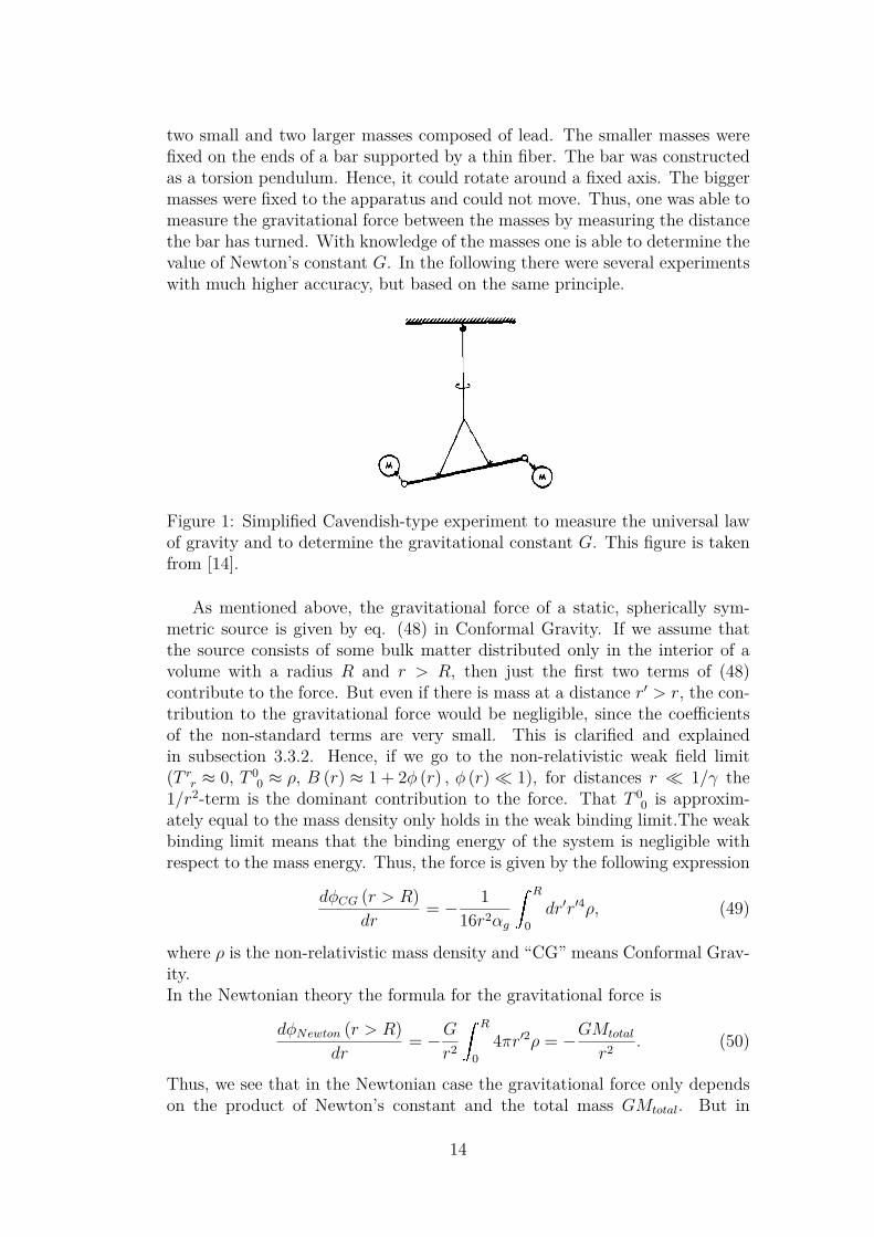
two small and two larger masses composed of lead. The smaller masses werefixed on the ends of a bar supported by a thin fiber. The bar was constructedas a torsion pendulum. Hence, it could rotate around a fixed axis. The biggermasses were fixed to the apparatus and could not move. Thus, one was able tomeasure the gravitational force between the masses by measuring the distancethe bar has turned. With knowledge of the masses one is able to determine thevalue of Newton’s constant G. In the following there were several experimentswith much higher accuracy, but based on the same principle.

Figure 1: Simplified Cavendish-type experiment to measure the universal lawof gravity and to determine the gravitational constant G. This figure is takenfrom [14].

As mentioned above, the gravitational force of a static, spherically sym-metric source is given by eq. (48) in Conformal Gravity. If we assume thatthe source consists of some bulk matter distributed only in the interior of avolume with a radius R and r > R, then just the first two terms of (48)contribute to the force. But even if there is mass at a distance r′ > r, the con-tribution to the gravitational force would be negligible, since the coefficientsof the non-standard terms are very small. This is clarified and explainedin subsection 3.3.2. Hence, if we go to the non-relativistic weak field limit(T rr ≈ 0, T 0

0 ≈ ρ, B (r) ≈ 1 + 2φ (r) , φ (r) 1), for distances r 1/γ the1/r2-term is the dominant contribution to the force. That T 0

0 is approxim-ately equal to the mass density only holds in the weak binding limit.The weakbinding limit means that the binding energy of the system is negligible withrespect to the mass energy. Thus, the force is given by the following expression

dφCG (r > R)dr

= − 116r2αg

R

0dr′r′4ρ, (49)

where ρ is the non-relativistic mass density and “CG” means Conformal Grav-ity.In the Newtonian theory the formula for the gravitational force is

dφNewton (r > R)dr

= −Gr2

R

04πr′2ρ = −GMtotal

r2 . (50)

Thus, we see that in the Newtonian case the gravitational force only dependson the product of Newton’s constant and the total mass GMtotal. But in

14

Conformal Gravity there is a so-called fourth-moment of the mass density ineq. (49). This means that the gravitational force does not only depend on thetotal mass Mtotal, but also on the matter distribution.

Therefore, it has been predicted there to be a problem [11], because in prin-ciple it should be possible to rule Conformal Gravity out by these Cavendish-type experiments. To see this, consider two homogeneous, spherically symmet-ric objects with the same total mass, but different mass densities. In NewtonianGravity the gravitational attraction should be the same, no matter which ob-ject is measured. But in Conformal Gravity the result should be different fordifferent mass distributions. For example if the radius of the first object is twotimes bigger than the radius of the second one, then the gravitational force ofthe first one will be four times bigger than the second one.

3.2.2 Circumvention of the Cavendish-type Problem

In this subsection we present the solution to the problem raised in 3.2.1 de-veloped by Mannheim and Kazanas [1, 11].

Experiments in the exterior region of some bulk matter yield that in theweak binding limit the coefficient of the gravitational force grows with thenumber of sources. Hence, the gravitational force of a macroscopic object isan extensive function of its microscopic constituents. Thus, it is sufficientto choose the mass density as the gravitational source. Hence, in the weakbinding limit it is sufficient to just sum over the potentials of the individualnuclei of the bulk matter

φ =N∑i=1

1∣∣∣~r − ~r′i∣∣∣ (51)

in Newtonian Gravity. To achieve this we can choose

g (r < R) =N∑i=1

mGδ (r − ri)

r2 (52)

in eq. (45). This choice of a point-like source is sufficient to yield a potential

φ = −NmGr

, (53)

but, in fact, it is not mandatory to choose a point-like potential to yield a1r-term.Let us make an important remark here. Although we always talk about

an interior solution for the regime r < R, this is not really an interior solu-tion in the sense of microscopic sources. It is just the interior of some bulkmaterial in a volume with the radius R. The gravitational potential of the mi-croscopic sources (protons, neutrons or atoms) itself is unknown and does nothave to be point-like. Everything we know is that the gravitational potentialpossesses a 1/r-behavior and that it grows linearly with the number density inthe weak binding limit. Therefore, every source, which yields these properties,is sufficient to be used as the gravitational source.

15

Although the Poisson equation also holds in the interior of the fundamentalmicroscopic source, there is no experimental data, since gravity is not thedominating force in this regime. Therefore, we are just insensitive to theinterior of the microscopic sources in the weak gravity and weak binding limit.Of course, in the interior of nuclei the explicit structure of the gravitationalsources would be important and one has to take into account the two-bodystrong coupling nuclear forces between the protons. Here the weak bindinglimit would not be an accurate approximation, because the fourth-momentintegral would not be proportional to the number density anymore. The sameholds for compact macroscopic objects like neutron stars. For these sources itis not sufficient to assume the weak binding approximation and it is necessaryto apply the complete equations (47) and (48). But actually also in standardgravity the strong binding limit is not tractable, since there is no reliable dataof this regime yet.

Now with this argumentation, in Conformal Gravity we are free to choosea microscopic source which is extended in space and has the following form

h (r < R) = −γN∑i=1

δ (r − ri)r2 − 3β

2

N∑i=1

[∇2 − r2

12∇4] [δ (r − ri)

r2

]. (54)

This source is positive definite and by explicit calculation one recognizes thatthe first term of eq. (54) only couples to the second-moment integral of eq.(47) or (48), whereas the second term just couples to the fourth-moment in-tegral. Therefore, the two coupling constants γ and β are indeed independentparameters. By explicit calculation we find β (2− 3βγ) = β and γ = γ. Byinserting this potential in eq. (47) we yield

φ (r > R) = −Nβr

+ Nγr

2 . (55)

The meaning of this special source is that one chooses a specific interior dis-tribution of the microscopic energy distribution to reproduce the Newtonian1/r-term and a term which is linear in r. Therefore, Mannheim was able tocircumvent the problem regarding the Cavendish-type experiments. But let usmention that actually it is not clear if this gravitational source is a physicalsource that represents the interior of protons. It just shows that, in principle,you can find sources that are adequate to circumvent the Cavendish-type prob-lem.

A remarkable fact is that within the theory of Conformal Gravity it ispossible to make predictions about the microscopic structure of a macroscopicsource by macroscopic measurements. This can be seen by assuming that theenergy density h is not like in eq. (54), but continuous. In consequence, thegravitational potential is given by

φ (r > R) = −NhR5

30r −NhR3r

6 . (56)

Thus, the ratio of the two contributions is proportional to R2, whereas thetwo parts of the gravitational potential in eq. (55), where we used (54) as the

16

gravitational source, are independent of each other. Therefore, if ConformalGravity appears to be the correct theory, one is able to state that the interiorof a macroscopic source is not continuous but rather discrete. For the stellarpotential (55) the ratio of the parameters is of the order

(β/γ

)1/2∼ 1023 cm,

which can be seen in 3.3 in eq. (90). So in the continuous case(β/γ

)1/2would

be of the order of the radius of a star, which is much smaller than 1023 cm.

3.3 Galaxy Rotation CurvesAs mentioned above, the additional term in the gravitational potential (47),which grows linearly with the distance, may be the reason for the fact that therotational velocities of stars in galaxies do not undergo the so-called Keplerianfall-off. To get an impression of the problem with the velocities of objects rotat-ing around a galaxy, let us make an estimate in the Newtonian limit of GeneralRelativity. A simplified calculation for a test particle in a static, sphericallysymmetric potential of a point mass M , where we equate the gravitationalforce and the centripetal force yields

vrot =√GM

r. (57)

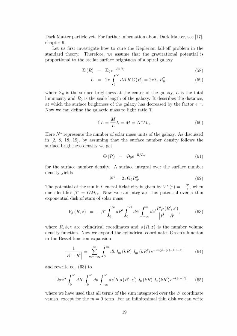
Here vrot is the rotational velocity of the particle. Hence, we notice that therotational velocity decreases like r−1/2 with growing distance. This expectedbehavior can be seen in fig. 2. The figure shows the measured data points forthe galaxy NGC 3198 and the theoretical curves for the Newtonian (dashed)and linear (dotted) potential. The sum of these contributions is depicted bythe solid line. It is quite obvious that there is a large discrepancy between themeasured data and the expected Keplerian fall-off for large distances. The ve-locities in the outer region seem to be systematically larger than the Keplerianexpectation, thus the curve just flattens on larger distances.

17

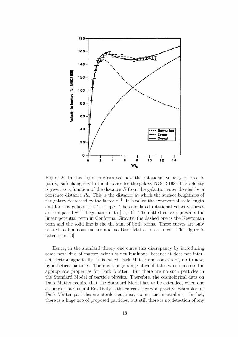
Figure 2: In this figure one can see how the rotational velocity of objects(stars, gas) changes with the distance for the galaxy NGC 3198. The velocityis given as a function of the distance R from the galactic center divided by areference distance R0. This is the distance at which the surface brightness ofthe galaxy decreased by the factor e−1. It is called the exponential scale lengthand for this galaxy it is 2.72 kpc. The calculated rotational velocity curvesare compared with Begeman’s data [15, 16]. The dotted curve represents thelinear potential term in Conformal Gravity, the dashed one is the Newtonianterm and the solid line is the the sum of both terms. These curves are onlyrelated to luminous matter and no Dark Matter is assumed. This figure istaken from [6]

Hence, in the standard theory one cures this discrepancy by introducingsome new kind of matter, which is not luminous, because it does not inter-act electromagnetically. It is called Dark Matter and consists of, up to now,hypothetical particles. There is a huge range of candidates which possess theappropriate properties for Dark Matter. But there are no such particles inthe Standard Model of particle physics. Therefore, the cosmological data onDark Matter require that the Standard Model has to be extended, when oneassumes that General Relativity is the correct theory of gravity. Examples forDark Matter particles are sterile neutrinos, axions and neutralinos. In fact,there is a huge zoo of proposed particles, but still there is no detection of any

18

Dark Matter particle yet. For further information about Dark Matter, see [17],chapter 9.

Let us first investigate how to cure the Keplerian fall-off problem in thestandard theory. Therefore, we assume that the gravitational potential isproportional to the stellar surface brightness of a spiral galaxy

Σ (R) = Σ0 e−R/R0 (58)

L = 2π ∞

0dRRΣ (R) = 2πΣ0R

20, (59)

where Σ0 is the surface brightness at the center of the galaxy, L is the totalluminosity and R0 is the scale length of the galaxy. It describes the distance,at which the surface brightness of the galaxy has decreased by the factor e−1.Now we can define the galactic mass to light ratio Υ

ΥL = M

LL = M = N∗M. (60)

Here N∗ represents the number of solar mass units of the galaxy. As discussedin [2, 8, 18, 19], by assuming that the surface number density follows thesurface brightness density we get

Θ (R) = Θ0e−R/R0 (61)

for the surface number density. A surface integral over the surface numberdensity yields

N∗ = 2πΘ0R20. (62)

The potential of the sun in General Relativity is given by V ∗ (r) = −β∗

r, when

one identifies β∗ = GM. Now we can integrate this potential over a thinexponential disk of stars of solar mass

Vβ (R, z) = −β∗ ∞

0dR′

2π

0dφ′

∞−∞

dz′R′ρ (R′, z′)∣∣∣~R− ~R′

∣∣∣ , (63)

where R, φ, z are cylindrical coordinates and ρ (R, z) is the number volumedensity function. Now we expand the cylindrical coordinates Green’s functionin the Bessel function expansion

1∣∣∣~R− ~R′∣∣∣ =

∞∑m=−∞

∞0

dkJm (kR) Jm (kR′) e−im(φ−φ′)−k|z−z′| (64)

and rewrite eq. (63) to

−2πβ∗ ∞

0dR′

∞0

dk

∞−∞

dz′R′ρ (R′, z′) J0 (kR) J0 (kR′) e−k|z−z′|, (65)

where we have used that all terms of the sum integrated over the φ′ coordinatevanish, except for the m = 0 term. For an infinitesimal thin disk we can write

19

ρ (R′, z′) = Θ (R′) δ (z′). Inserting this number volume density in eq. (65)yields

Vβ (R) = −2πβ∗ ∞

0dk

∞0

dR′R′Θ (R′) J0 (kR) J0 (kR′) (66)

in the z = 0 plane. We use the following identities for Bessel functions ∞

0dRRJ0 (kR) e−αR = α

(α2 + k2)3/2 , (67) ∞

0dk

J0 (kR)(α2 + k2)3/2 = R

2α

[I0

(Rα

2

)K1

(Rα

2

)− I1

(Rα

2

)K0

(Rα

2

)](68)

and by choosing α = 1/R0 we find

Vβ (R) = −πβ∗Θ0R[I0

(R

2R0

)K1

(R

2R0

)− I1

(R

2R0

)K0

(R

2R0

)]. (69)

Then by using further the Bessel function relations

I ′0 (x) = I1 (x) , I ′1 (x) = I0 (x)− I1 (x)x

, K ′0 (x) = −K1 (x) , (70)

K ′1 (x) = −K0 (x)− K1 (x)x

and differentiating eq. (69) one finds

V ′β (R) = N∗β∗R

2R30

[I0

(R

2R0

)K0

(R

2R0

)− I1

(R

2R0

)K1

(R

2R0

)]. (71)

Now for a test particle moving on a circular orbit around a massive body wecan use the Virial theorem

v2 = RV ′. (72)Here v represents the rotational velocity of the particle and V is the potentialof the central mass. By combining (71) and (72) we get the rotational velocityof the luminous matter

v2lum = RV ′β (R) = N∗β∗R2

2R30

[I0

(R

2R0

)K0

(R

2R0

)− I1

(R

2R0

)K1

(R

2R0

)]. (73)

In the R R0 limit this expression simplifies to

v2lum →

N∗β∗

2R

(1 + 9R2

02R2

)→ N∗β∗

2R . (74)

In fig. 2 we see that there is an initial increase of the rotational velocityfrom R = 0 to R ≈ 3R0 for the Newtonian term and after that it steadily falls.This behavior is represented by eq. (73) and this result fits nicely with oursimplified calculation, cf. (57), where we assumed that the galaxy is a pointmass.

For a more accurate calculation one has to take into account that thegalactic disk has a finite thickness and that the HI gas has its own surface

20

brightness. Furthermore, some galaxies have a central bulge. This more de-tailed calculation is given in [2, 19].

As one can see in fig. 2 the luminous matter fits the data in the innerregion quite well, but in the outer region it yields much to low values forrotational velocities. To cure this discrepancy one can assume that there issome additional non-luminous matter distribution. Conventionally, one takesthe spherical Dark Matter distribution σ (r) to be an isothermal Newtoniansphere in hydrostatic equilibrium

σ (r) = σ0

(r2 + r20) , (75)

where r0 denotes the radius of an inner core to prevent the distribution fromdiverging at r = 0. The integration of the Newtonian potential over this DarkMatter distribution results in a rotational velocity of the following form [2]

vdark = 4πβ∗σ0

[1− r0

Rarctan

(R

r0

)], (76)

vdarkRr0→ 4πβ∗σ0. (77)

This yields an asymptotically flat curve, but nonetheless a simple addition ofvlum and vdark does not fit the observed rotation curves automatically. HereMannheim claims [2] that one has to adjust the two free parameters σ0 andr0 for every galaxy. But this seems to be natural, since each galaxy has adifferent mass, merger history and age. Therefore, the galaxies are in differentphases of their evolution. Nevertheless one has to fine-tune the Dark Matterdistribution to solve the problem of the galactic rotation curves.

3.3.1 Universality in the Data

In [19] it is pointed out that the data of rotational velocities of galaxies exhibita universality. In this section we want to present this universal behavior of therotational velocities and in section 3.3.2 we show how this universality matchesto Conformal Gravity.

One can separate the measured galaxies in three categories. The first aregalaxies of low luminosity, for which the rotational velocity generally still raisesat the last data points. For intermediate to high luminosity galaxies the velo-city seems to be flat and those for highest luminosity galaxies to be (slightly)falling. In [20] Mannheim investigated a subset of 11 galaxies for which therange of luminosity differs by a factor of about 1000, see tab. 1 in the Appendix.From fig. 6 in the Appendix the lack of flatness for the first four diagrams ofgalactic rotation curves is quite obvious, but it is commonly assumed that alsothese rotational velocities will flatten for larger distances. Further, there isone special feature for the galaxy DDO 154, for which the curve turns overand falls after some distance. The reason for this could be that this galaxy isthe most gas dominated of the sample and random gas pressure could make alarge contribution to the velocities in the turn over region. However, in [18]

21

Mannheim states that this fall of the rotation curve is not apparent in themore recent THINGS survey of the galaxy.

Mannheim points out that it could be more instructive to investigate thevelocity discrepancy rather than the total velocity, i.e. to look at the excess ofthe actual velocity over the Newtonian contribution. This discrepancy clearlyraises with the distance for the last detected data points, as can be seen infig. 2.

Furthermore, for the flat rotation curve galaxies there is a regularity in themagnitude of the luminosity. One finds a phenomenological relation betweenthe luminosity and the rotational velocity to the power of four. This relationis called the Tully-Fisher law [21]

L ∝ v4. (78)

This means that if one knows the rotational velocity of a galaxy one can predictthe Luminosity of that galaxy. Thus, by measuring the apparent brightnessone can calculate the distance of the galaxy.

Another universality is given by the fact that the brighter spiral galaxiesseem to have a common central surface brightness ΣF

0 . Freeman [22] was thefirst, who recognized this. But this common central surface brightness doesnot hold for all galaxies of lower luminosity.

In consequence, it is interesting to investigate a universality which is presentfor all three categories of galaxies. From tab. 1 we see that the quantity(v2

c2R

)tot, which represents the centripetal acceleration at the last data point,

varies just by a factor of 5. After subtracting the Newtonian contribution thequantity

(v2

c2R

)net

even only varies by a factor of 4, although the luminosityof the galaxies varies by a factor of 1000. Besides that, we recognize that therotational velocity slightly increases with increasing mass.

Note that the last measured data point of the galaxy is only fixed bythe instrumental limit and not by any dynamics of the galaxy. Therefore,it is completely arbitrary. The range of the distances of the last detectedpoints runs roughly from 8 kpc to 40 kpc. Thus, because

(v2

c2R

)net

is roughlyconstant this immediately leads to the suggestion that v2 grows universally andlinearly with R. This means that the rotational velocity is not permitted todepend strongly on any galaxy specific quantity like N∗. This seems to be veryspeculative, since Mannheim just pics a small number of galaxies out of thepresumably ∼ 1011 galaxies in the observable Universe. However, Conformalgravity is able to account for this hypothetically universal behavior. This isexplained in subsection 3.3.2.

3.3.2 Fit with a Linear Potential Term

As we have pointed out before, the introduction of Dark Matter is not the onlypossibility to cure the problem with the mass discrepancy for galactic rotationcurves. Mordehai Milgrom [22] suggested a theory in 1983 called “ModifiedNewtonian Dynamics” (MOND), which modifies Newton’s second law for smallaccelerations. Therefore, in the regime of small accelerations Newton’s second

22

law behaves like F = ma2

a0and this yields a constant rotation velocity for the

stars in the outer region of a galaxy.Besides that, Conformal Gravity provides a simple, but still viable solution

to the fact that the rotation curves do not follow the expected Keplerian fall-off, but mostly flatten or just slightly increase in the outer region.

Remember eq. (73), which gives the rotational velocity just for luminousmatter. We will repeat the same calculation, but now with an additional termlinear in R [2, 18, 19]. The potential produced by the sun changes to

V ∗CG (R) = −β∗

R+ γ∗R

2 , (79)

Hence, we are able to generalize the formalism to calculate the rotationalvelocity of stars in Conformal Gravity. Therefore, we set

∣∣∣~r − ~r′∣∣∣ = (~r−~r′)2

|~r−~r′| andby using the second term of eq. (79) we immediately find

Vγ (R, z) = γ∗

2

∞0

dR′ 2π

0dφ′

∞−∞

dz′R′ρ (R′, z′) (80)

×(R2 +R′2 − 2RR′ cos (φ′) + (z − z′)2

)1/2

= πγ∗ ∞

0dk

∞0

dR′ ∞−∞

dz′R′ρ (R′, z′)

×[(R2 +R′2 + (z − z′)2

)J0 (kR) J0 (kR′)− 2RR′J1 (kR) J1 (kR′)

]e−k|z−z

′|

Again, for an infinitesimally thin disk at z = 0 we find

Vγ (R) = πγ∗ ∞

0dk

∞0

dR′R′Θ(R′)

(81)

×[(R2 +R′2

)J0 (kR) J0

(kR′

)− 2RR′J1 (kR) J1

(kR′

)].

With eq. (67) and eq. (68) and the relation∞

0 dR′R′2J1 (kR′) e−αR = 3αk(α2+k2)5/2

we can write

Vγ (R) = πγ∗Θ0RR20

[I0

(R

2R0

)K1

(R

2R0

)− I1

(R

2R0

)K0

(R

2R0

)](82)

+πγ∗Θ0R

2R0

2

[I0

(R

2R0

)K0

(R

2R0

)− I1

(R

2R0

)K1

(R

2R0

)]and the by differentiation with respect to R and using eq. (70) we find

RV ′γ (R) = N∗γ∗R2

2R0I1

(R

2R0

)K1

(R

2R0

). (83)

Combining this with eq. (73) the local contribution of the luminous matterreads

v2lum = N∗β∗R2

2R30

[I0

(R

2R0

)K0

(R

2R0

)− I1

(R

2R0

)K1

(R

2R0

)](84)

+N∗γ∗R2

2R0I1

(R

2R0

)K1

(R

2R0

)

23

and in the limit for large R we get

v2lum

RR0→ N∗β∗

R+ N∗γ∗R

2 . (85)

We recognize that we produced two terms, which contribute to the rotationalvelocity that depend on the number of stars N∗. Hence, these contributionsdepend on the galaxy itself.

Now let us think about a major difference between Newtonian Gravity andConformal Gravity. In Newtonian Gravity it is very familiar to us that justthe matter interior of the volume given by a ball with the radius r of theobservers position contributes to the gravitational potential. The rest of theUniverse does not contribute. But this behavior is only valid for sphericallysymmetric 1

r-potentials, thus it does not hold in Conformal Gravity anymore.

As we mentioned before in 3.2, by this reason Newtonian Gravity is simply alocal theory, whereas Conformal Gravity is a global theory. And, indeed, thereare contributions to the rotational velocity from the rest of the Universe, i.e.contributions that are universal and do not depend on the morphology, size,luminosity or mass of the galaxy, just as was pointed out in 3.3.1.

Hence, as the Universe consists of a homogeneous and isotropic backgroundand large scale inhomogeneities like galaxy clusters and superclusters we havetwo global contributions to the rotational velocity.

For the background part of the Universe we usually assume a Robertson-Walker (RW) geometry

ds2 = −dt2 + a2 (τ)(1 + Kρ2

4

)2

(dρ2 + ρ2dΩ2

). (86)

This is a Robertson-Walker line element in isotropic coordinates. It is homo-geneous and isotropic and thus conformal to a flat geometry. Hence, after aappropriate coordinate transformation it is also a solution to the static, spher-ically symmetric equation (39). The Weyl tensor (10) and W µν (19) vanish inthis geometry. Consequently, also the matter energy-momentum tensor T µνMin eq. (20) has to vanish. Therefore, the background does not contribute tothe inhomogeneous Bach equation (39). But there is a contribution to thehomogeneous equation ∇4B (r) = 0, when W µν vanishes non-trivially. Hence,this forces T µν to vanish non-trivially, i.e. by a positive contribution of thematter sources and a negative contribution of the gravitational part. This isindeed possible if the 3-curvature K is negative. In chapter 6 we will see thatthis is feasible in Conformal Gravity. Thus, in the following we want to lookat this term in detail.

The cosmological Hubble flow is the motion of astronomical objects due tothe expansion of the Universe. It is described in comoving coordinates whichare given by eq. (86). But the galactic rotational velocities are measured ina coordinate system which is fixed to the center of the galaxy, i.e. the galaxyis at rest. Therefore, we have to find the transformation between these two

24

coordinate systems. Explicitly it is given by

r = ρ(1− γ0r

4

)2 , τ =dtR (t) . (87)

Therefore, the RW line element changes in the following way

Ω2 (τ, ρ)

−dτ2 + R2 (τ)[1− γ2

0ρ2

16

]2(dρ2 + ρ2dΩ2)

(88)

=

(1+ γ0ρ

41− γ0ρ

4

)2

R2 (τ)

−dτ2 + R2 (τ)[1− γ2

0ρ2

16

]2(dρ2 + ρ2dΩ2)

= − (1 + γ0r) dt2 + dr2

(1 + γ0r)+ r2dΩ2,

where Ω2 (τ, ρ) = 1R2(τ)

(1+ γ0ρ

41− γ0ρ

4

)2is the conformal factor, but dΩ2 is the angular

part of the line element of the spherical coordinates. Thus, after a conformaltransformation a RW geometry written in a static coordinate system is equival-ent to a static line element with a universal linear term γ0r. Since the spatial3-curvature of these coordinates K = −γ2

04 is negative, γ0 has to be real. This is

necessary for the γ0R2 term to be able to serve as a potential. Hence, in analogy

to the calculation for the linear term of eq. (79) and because the rotationalvelocities are non-relativistic we can simply add this contribution to eq. (85)and yield

v2 RR0→ v2lum + γ0R

2 = N∗β∗

R+ N∗γ∗R

2 + γ0R

2 . (89)

With this formula the data of 11 galaxies were fitted [20]. The first two termsare galaxy dependent, because they contain N∗. But the third term is univer-sal and linear. This is the term, as Mannheim argues, which represents theuniversality we explained in 3.3.1. It is totally luminosity independent andtherefore on a very different footing than the other two terms. The fit yieldsfor the parameters [1]

β∗ = 1.48× 105cm, γ∗ = 5.42× 10−41cm−1, γ0 = 3.06× 10−30cm−1. (90)

Here one also gets a quantitative answer to the question whether the SolarSystem is influenced by this linear modifications to the rotational velocities.We recognize that the parameter γ∗ is small and therefore N∗γ∗ ∼ 10−30 cm−1

is still a very small quantity. Only on the length scales of galaxies (R ∼ 10 kpc)the linear contributions become of the order of the Newtonian contribution.Thus, on Solar System distances (R 10 kpc) the linear term is negligible.

Additionally the value for γ0 indicates that it is of cosmological magnitude,since it is of the order of magnitude of the inverse Hubble radius. So if thetheory turns out to be correct, then it also provides a possibility to measurethe spatial 3-curvature of the Universe. On top of that, in Conformal Gravitythere is only one free parameter per galaxy, namely the optical disk mass to

25

light ratio Υ or equivalently the total amount of stars or gas in the galaxy,N∗, in solar mass units. Hence, no fine-tuning of parameters is necessary inConformal Gravity.

Now let us turn to the mentioned universality in the data. The localcontribution N∗γ∗

2 varies enormously with the luminosity, i.e with N∗. Butstill the global contribution dominates

(v2

c2R

)net

and it only slightly dependson the galactic mass or luminosity. Except for the largest galaxies, for whichN∗ is of the order of the critical mass Ncrit = 5, 65 × 1010. Here the localcontribution is of the order of the global one, see Appendix tab. 1.

With this theory we are also able to explain, why the low luminosity galax-ies do not flatten. For these galaxies N∗ is much lower than Ncrit and alsoΣ0 is so low that the global γ0-term immediately wins against the local con-tributions and the rotation curves raise from the beginning. For the largestgalaxies where N∗ is greater than Ncrit the local contribution is temporarilylarger than the global contribution, but after that it slightly falls and in theend the linear contribution wins, see tab. 1, NGC 2841. Note that the data ofthis galaxy goes to much larger distances.

As mentioned above, there is still another contribution from the rest of theUniverse. In [19, 24] Mannheim states that inhomogeneities contribute to ther2-term in eq. (48). These inhomogeneities are typically clusters and super-clusters of galaxies. Their distance scale ranges from 1 Mpc up to about 100Mpc. Mannheim argues that the integral of the r2-term is constant, if we as-sume that the integral is evaluated between fixed endpoints. And furthermore,Mannheim assumes that the lower integration limit begins at some rcluster thatis larger than the radius of the galaxy and independent of it. Therefore, onscales r < rcluster and by introducing the constant κ = 1

3

∞rclust

dr′r′h (r′) onefinds the following approximate formula in the weak gravity and asymptoticlimit

v2TOT

RR0→ N∗β∗

R+ N∗γ∗R

2 + γ0R

2 − κR2. (91)

It is important to mention here that such a form can be achieved by startingwith a metric term B (r) = −κr2. This term has the de Sitter-like form, butit can’t be associated with a de Sitter geometry, because the inhomogeneitiesare not distributed maximally 4-symmetrically. Anyway, a test particle wouldbe influenced by that r2-term and therefore the result is the same as if it hadbeen embedded in a de Sitter geometry. But this whole argumentation is atleast questionable, because there is no spherical symmetry on these distancescales.

At the time when eq. (89) was fitted to the set of 11 galaxies the datadid not go to so far distances. Therefore, the fits of the galactic rotationcurves without the r2-term were perfectly in line with the data. But in thefollowing, when there was data available to further distances, it seems thatthe rotation curves were not raising anymore, but staying more or less flat,see fig. 7. Hence, only with the additional r2-term one was able to repro-duce this feature of the rotation curves. With a new data set of 111 galaxies21 galaxies were found, in which the expectation of eq. (89) totally overruns

26

the data points for large distances [10, 19]. Consequently, these 21 galax-ies were fitted with the repulsive term −κR2. By doing so the value of theparameter κ = 9, 54 × 10−54 cm−2 ≈ (100 Mpc)−2 was fixed and flat galacticrotation curves for larger distances could be reproduced. The fitting of theother 90 galaxies was unaffected by this new term, see [19, 24]. Because thequadratic term eventually will dominate, eq. (91) will become negative atsome distance. But v2

TOT cannot be negative. Therefore, beyond the distanceR ∼ (N∗γ∗ − γ0) /2κ ∼ 100 kpc for N∗ = γ0/γ

∗ = 5, 56×1010 there cannot beany bound circular orbits. By this fact, a galaxy terminates naturally at thisdistance scale.

Despite this effective fitting mechanism for galactic rotation curves, stillthere are at least three arguments for the existence of Dark Matter. These arethe cosmic growth of structures (see chapter 7 in [25]), Dark Matter in galaxyclusters measured by strong lensing and the Bullet clusters [26]. It seems thatthese indications for Dark Matter are hard to explain for Conformal Gravity.Nevertheless, Conformal Gravity does not completely exclude the existence ofDark Matter. It is still possible to have some kind of Dark Matter in ConformalGravity, which could lead to a solution to these issues.

In this chapter we applied the macroscopic equations of the theory of Con-formal Gravity to solve the Dark Matter problem. Now in the next chapterwe want to turn to the microscopic side of the theory to investigate the zeropoint energy problem and the quantization of gravity.

4 QuantizationThis chapter deals with the quantization in the theory of Conformal Gravity.We will mainly follow the discussion in [1, 3, 27, 28].

The reason to seek a viable theory of quantum gravity is that there aresituations in the Universe where gravity and quantum effects are equally im-portant. For example such a situation was the beginning of the Universe. Weactually think, in the standard Big Bang models, that the Universe began in aspace-time singularity. This means there was a boundary of space-time. Theenergy density of the Universe was very large and the matter was so stronglycompressed that quantum-mechanical effects should play a significant role. An-other example are Black Holes, which also represent a space-time singularity.The crucial point is that the standard theory of gravity, namely General Re-lativity, does not include the laws of quantum mechanics and is treated purelyclassical. It is commonly assumed that the Einstein equations break downwhen quantum effects become important. So to describe the above mentionedsituations, one has to come up with a theory of quantum gravity.

There are several approaches to quantum gravity like String Theory orLoop Quantum Gravity, but there is no consensus of which of these theories,if any, is the correct theory for describing quantum gravitational effects, yet.

Thus, let us see how Conformal Gravity treats this problem. The actionof Conformal Gravity is scale-free on the fundamental level. This means thatinitially there are no length or mass scales in the theory. How mass is produced

27

in the theory of Conformal Gravity is the topic of chapter 5 and in this chapterwe will focus on how the zero-point problem and the problem with the cosmo-logical constant can be cured in Conformal Gravity. So since there is no lengthscale, we can state that on this fundamental level the only allowed geometryfor macroscopic Conformal Gravity is the flat Minkowski space. Mannheimargues this in [1] as follows. If there are no length scales, there is nothing todefine curvature, because one always has to compare curvature to a certainlength. So if we take W µν to be a classical function, eq. (37) is an exteriorvacuum solution to W µν = 0, but there is no reason for taking the dimen-sionful parameters β, γ or k to be non-zero. Therefore, we will see that therehas to be some symmetry breaking in order to yield a solution which has lesssymmetry than the differential equation itself. Now, if all of that symmetrybreaking is produced quantum-mechanically, then in the classical case space-time has to be flat. Thus, mass in the Schwarzschild solution that is producedquantum-mechanically generates also curvature by a quantum-mechanical pro-cess. Explicitly, the commutation relations produce the length scales in thetheory. This can be seen by the fact that a commutation relation of the form[

φ (~x, t) , π(~x′, t

)]= i~δ3

(~x− ~x′

)(92)

produces a delta function, which is a non-linear relation and is thus not scale-invariant. φ (~x, t) denotes some quantum field and π (~x, t) is its momentumconjugate.

When one quantizes General Relativity usually one expands the metricin a power series of the gravitational coupling constant G, but in ConformalGravity one has to expand the metric in a power series of Planck’s constant~, because by the above argumentation quantum mechanics is an indicator forthe deviation from flat space-time. Nevertheless, one cannot use the standardcanonical quantization mechanism. The reason for this is that the gravita-tional field is the space-time metric gµν itself. So for the matter fields one candefine an energy-momentum tensor T µνM by varying the matter action IM withrespect to the metric. Besides that, one yields the field equations for a matterfield φ, when one varies the matter action with respect to the associated field.Furthermore, the field equations are constrained by the stationarity conditionof the Hamilton’s principle. This says that one yields the field equation whenthe deviation of the action with respect to the field is zero, i.e. δIM

δφ= 0. Then

the field equation is constrained, but the matter energy-momentum tensoris not. Now for gravity the situation is different. For the field equation ofgravity we also have to vary with respect to the metric, since the metric isthe gravitational field. But as there is the constraint for the field equationfrom δIGRAV

δgµν= 0, then also the energy-momentum tensor is constrained, i.e.

δIGRAVδgµν

≡ T µνGRAV = 0. So in the absence of a coupling between matter andgravity, gravity is still coupled to itself. This does not result in a problem aslong as we treat gravity purely classical. But when one wants to quantize grav-ity one gets into trouble. To clarify this, consider the Einstein equations (7).To be an operator identity both sides have to be either classical or quantummechanical. On the one hand gravity is not well defined quantum mechanic-

28

ally, because radiative corrections are possibly not renormalizable, but on theother hand the matter side consists of quantum fields. Therefore, one assumesa semi-classical form of the Einstein equations

18πGG

µνCL = −〈Q|T µνM |Q〉 , (93)

where GµνCL =

(Rµν − 1

2gµνRα

α

)CL

denotes the classical Einstein tensor and〈Q|T µνM |Q〉 is a c-number matrix element in the quantum state |Q〉. So basic-ally one replaces the matter energy-momentum tensor T µνM by its expectationvalue. But still the expectation value contains products of fields at the samepoint. Thus, its matrix elements are not finite and one has to subtract theinfinities by hand. In the standard theory it is not clear why this is correct,because actually gravity couples to the full energy-momentum tensor and notjust to energy differences. So conventionally, one uses the following form ofthe Einstein equations

18πGG

µνCL = − (〈Q|T µνM |Q〉 − 〈Ω|T

µνM |Ω〉DIV ) = −〈Q|T µνM |Q〉FIN . (94)

|Ω〉 denotes the matter field vacuum state. So for example to describe a blackbody like the cosmic microwave background one uses an ensemble average overan appropriate set of positive-energy Fock space states. These are eigenstatesto the Hamilton operator

∑ω(a†(~k)a(~k)

+ 12

)(95)

and one simply neglects the ∑ω/2 zero-point contributions.So now that we have an idea of the problems with quantum gravity in

General Relativity, we continue with Conformal Gravity and its solution tothese problems. As we have explained above, it is not possible to quantizegravity alone. Therefore, if we impose stationarity not just on T µνGRAV alone,but on the energy-momentum tensor of the whole Universe

T µνUNIV = T µνGRAV + T µνM = 0, (96)

we can cancel the zero-point energy contributions consistently. This is becauseConformal Gravity is renormalizable, since the gravitational coupling constantαg in (9) is dimensionless. In contrast, for General Relativity it is unclear ifit could be a finite theory. When gravity is quantized it is now possible tohave a non-zero T µνGRAV , because it is coupled to the matter energy-momentumtensor T µνM . But to achieve this cancellation of the vacuum contributions, thecommutation relations must have a form that depends on the commutationrelations of the matter fields. Therefore, gravity is quantized through thecoupling to matter and additionally, the gravitational commutation relationsare also fixed by the coupling to matter.

In Conformal Gravity we can use a boson-fermion cancellation. In [1]Mannheim assumes assumes that this cancellation takes place due to the fact

29

that bosons and fermions contribute with different signs to the vacuum energy.Thus, since gravitational quanta are bosonic one can achieve a cancellationbetween the gravitational and the matter field parts. For such a cancella-tion one needs three things: a symmetry, fermions in the matter field sectorand a theory which is renormalizable. All of these conditions are fulfilled inConformal Gravity and hence, in the following it will be explained how thecancellation takes place.

The following expansion of (96) follows the argumentation in [1]. Alreadyin flat space-time there are zero-point and cosmological constant contributions,and since gravity is absent in flat space-time it cannot be responsible for it.Thus, the way to solve this problem is to put gravity on an equal footing withthe matter field sector. This is done by the fact that the Bach equations arepurely quantum mechanical equations what means that gravity and the matterfield sector are treated only microscopically. So as was pointed out above, weexpand the metric in a power series of ~. The lowest order quantum-mechanicalcontribution to T µνM is a zero-point contribution of order ~. Thus, to cancelthis contribution also the lowest order of the gravitational part has to be ~.Since the zero-point contribution is due to products of fields at the same point,the order ~ contribution to the gravitational vacuum part has to consist of aproduct of two gravitational fields. Hence, it is given by varying the part of thegravitational action in eq. (9), which is second-order in the metric perturbationhµν with |hµν | 1,

IW (2) = −αg2

d4x hµν hµν , (97)

i.e. by−4αgW µν (2) ≡ T µνGRAV . (98)

One can evaluate T µνM in flat background, because it is already of order ~and a non-flat metric gµν would produce a matter energy-momentum tensorof higher order in ~. So an energy-momentum tensor in flat background willgenerate curvature of order ~. This means that the ~2 term in T µνM is curvaturedependent, because it contains the non-flat metric. Additionally, the zero-pointcancellation in eq. (96) will occur to all orders in ~. Hence, one can decomposethe gravitational and matter contribution into finite and divergent parts, whichlead to

(T µνGRAV )DIV + (T µνM )DIV = 0, (99)

and(T µνGRAV )FIN + (T µνM )FIN = 0. (100)

So there is no need for a renormalization of the individual terms, since theterms regulate each other and thus their sum is finite. In consequence, weare allowed to work with eq. (100) alone, because all infinities have beenremoved. This has a decisive consequence for the gravitational fluctuationshµν in Conformal Gravity. Since W µν (2) is of order ~ and contains products

30

of two gravitational fields, the gravitational field has to be of order ~1/2. Thismeans that the Bach equations to lowest order read

−4αgW µν (1) = 0, (101)

since W µν (1) is of order ~1/2, but the lowest order of T µνM is of order ~. Hence,this provides Conformal Gravity with a wave equation, which is strictly ho-mogeneous. This is totally different to standard gravity, where one expands ina power-series of the gravitational coupling constant G. There the first-ordergravitational fluctuation is produced by a first-order matter source. Eq. (101)does not permit hµν to be non-zero, but because of the second-order equation

−4αgW µν (2) + T µνM = 0 (102)

the fluctuation has to be non-trivial.Lastly, let us note that the operator identity 〈Ω|T µνGRAV |Ω〉+〈Ω|T

µνM |Ω〉 = 0

does not only hold for the matter vacuum state |Ω〉, but also after symmetrybreaking in some spontaneously broken vacuum |ΩM〉

〈ΩM |T µνGRAV |ΩM〉+ 〈ΩM |T µνM |ΩM〉 = 0. (103)

This means that in the case of mass generation and an induced cosmologicalconstant, all the various zero-point contributions have to readjust in such a waythat the cancellation still occurs after the spontaneous symmetry breaking.Thus, Mannheim states in [1, 2, 3] that one has to treat the cosmologicalconstant in conjunction with the zero-point energies. Hence, this providesa possibility to solve the cosmological constant problem, because there is aconstraint for the cosmological constant by this requirement as we we will seein chapter 5 and 6.

The explicit cancellation of these zero-point contributions and the cosmo-logical constant is done in [1, 3].

31

5 Mass GenerationThis chapter deals with the generation of mass in Conformal Gravity. Initiallythere is no bare mass term on the level of the matter action IM . The reasonfor this is that a mass term would introduce a mass scale to the theory, but aconformal invariant theory is not permitted to have a mass scale on the levelof the action. This can also be seen by the fact that an energy-momentumtensor, which results from a conformal invariant action, has to be tracelessand such a mass term would destroy the traceless property of the energy-momentum tensor. Mathematically this means that the action would not beinvariant under a conformal transformation (11). But since we know fromexperiment that Standard Model particles indeed have a mass, we have to finda mechanism which is responsible for the particle physics matter to acquiresome mass. That one is not allowed to start with a mass term on the levelof the action is not a problem, since even in the Standard Model of particlephysics masses are produced via the Higgs mechanism. The discussion in thischapter follows [1] and chapter 3 in [2].

5.1 The Energy-Momentum Tensor of Test Particles andPerfect Fluids

At the time when General Relativity was introduced there was no QuantumField Theory established. The matter fields were assumed to consist of hard“billiard balls” like purely mechanical kinematic particles, which are providedwith energy and momentum. However, today it is clear from the StandardModel of particle physics (SU (3)×SU (2)×U (1) theory of strong, weak andelectromagnetic interactions) that matter as the source of gravity has to betreated as fields and no longer as hard “billiard balls”. But the kinematicalenergy-momentum tensor is still used as the source of gravity, because it leadsto geodesic motion, which is well confirmed by experiment. This is a short-coming we will overcome below in this chapter and we will justify, why it issufficient to work with the energy-momentum tensor of test particles or perfectfluids.

So let us start with the energy-momentum tensor for test particles whichis given by

2√−g

δITδgµν

= T µν = m√−g

dτδ4 (x− y (τ)) dy

µ

dτ

dyν

dτ, (104)

Now by using the covariant energy-momentum conservation T µν;ν = 0 onerecovers the geodesic equation (2).

For the energy-momentum tensor of the form of a perfect fluid

T µνF luid = [(ρ+ p)uµuν + gµνp] , (105)

where ρ is the relativistic mass density and p is the pressure. uµ is the fourvelocity, which obeys uµuµ = −1 with our sign convention for the metric.

32

The covariant conservation for a perfect fluid can be written in the followingform

[(ρ+ p)uµuν + gµνp];ν = [(ρ+ p)uν ];ν uµ + (ρ+ p)uµ;νuν + p;µ = 0. (106)

The semicolon represents a covariant derivation, whereas the comma denotesa partial derivative. With uµuµ;ν = 0 and by multiplying eq. (106) with uµ wecan conclude

− [(ρ+ p)uν ];ν + p;µuµ = − (ρ+ p)uµ;νuνuµ = 0. (107)

So if we insert eq. (107) in eq. (106) we find

(ρ+ p)uµ;νuν + p;ν [gµν + uµuν ] = 0. (108)

Now by dividing eq. (108) by (ρ+ p) and rewriting the covariant derivativewe yield

D2xµ

Dτ 2 = − [gµν + uµuν ] p;ν

(ρ+ p) . (109)

Here we see that we reproduce the geodesic equation when the right-handside of (109) is negligible. E.g. this situation is achieved for non-interacting,pressureless dust.

It is obvious now why one naturally assumes that the sources of gravityshould be described by test particles or a perfect fluid, because both lead togeodesic motion.

Nevertheless, it is still possible to add a term T µνextra to the energy-momentumtensor, which is covariantly conserved independently. Thus, it would notchange the equation of motion (109). Therefore, one can add a termT µνextra = Gµν to the total energy-momentum tensor, because the Einstein tensoris covariantly conserved on its own and non-existent in flat space-time. Be-sides that, the same holds for the metric tensor, which is covariantly conserved,∇µg

µν = 0, too. Hence, we can include a term gµνΛ, where Λ is a constant,leaving eq. (109) unaffected. Such a term would lead to an unobservable shiftin the zero of energy in flat space-time.

In conclusion we can say that the energy-momentum tensor of a perfectfluid is sufficient to yield geodesic motion, but it is not at all necessary. Wewill show this in more detail in the next section 5.2 and use this in chapter 6to cure the cosmological constant problem.

5.2 Dynamical Mass GenerationNow, let us investigate why it is sufficient to work with test particles andperfect fluids, although we know that the matter part consists of fields ratherthan particles.

Therefore, we analyze the structure of the energy-momentum tensor forelementary particles whose masses are produced dynamically, i.e. they acquiremass by spontaneous symmetry breaking.

33

We consider a massless spin one-half matter field fermion ψ (x), which getsits mass via a real spin-zero Higgs scalar boson field S (x). So we start withan action which does not contain any kinematic mass scale. Furthermore, tomaintain the tracelessness of the energy-momentum tensor, the scalar field iscoupled conformally to the curvature. Hence, we can write down a curved-space matter action

IM = −d4x√−g

[S,µS,µ

2 −S2Rµµ

12 + λS4 + iψγµ (x) [∂µ + Γµ (x)]ψ − hSψψ], (110)

where h and λ are dimensionless coupling constants and Γµ (x) is the fer-mion spin connection. This action IM is the most general action, whichis not only local coordinate invariant, but also invariant under local Weyltransformations of the form S (x) → e−α(x)S (x), ψ (x) → e−3α(x)/2ψ (x) andgµν (x)→ e2α(x)gµν (x). A crucial difference between test particles and fields isthat for fields the geodesic motion is not achievable just by the covariant en-ergy conservation. Rather we have to use some equation of motion for the fielditself. This means that there is additional dynamical information contained inthe equation of motion of the matter fields. Therefore, by varying eq. (110)with respect to S (x) and ψ (x) we find the field equations

S,µ;µ + 16SR

µµ − 4λS3 + hψψ = 0, (111)

iγµ (x) [∂µ + Γµ (x)]ψ − hSψ = 0. (112)The energy-momentum tensor can be obtained by variation of eq. (110) withrespect to the metric

TMµν = iψγµ (x) [∂ν + Γν (x)]ψ + 2S,µS,ν3 − gµνS

,αS,α6 − SS,µ;ν

3 +gµνSS

,α;α

3 (113)

−16S

2[Rµν −

12gµνR

αα

]− gµν

[λS4 + iψγα (x) [∂α + Γα (x)]ψ − hSψψ

].

Now, we multiply eq. (112) with ψ and eq. (111) with gαβS and isolate the−4gαβλS4 term to bring the energy-momentum tensor in the following form

TMµν = iψγµ (x) [∂ν + Γν (x)]ψ + 2S,µS,ν3 − gµνS

,αS,α6 − SS,µ,ν

3 (114)

+gµνSS

,α,α

12 − 16S

2[Rµν −

14gµνR

αα

]− gµνhSψψ

4 .

One can explicitly calculate the tracelessness(T µM µ = 0

)and the covariant

conservation(T µνM ;ν = 0

)of this energy-momentum tensor by employing the

field equations of motion again. Therefore, we see that the structure of thisenergy momentum tensor is extremely different from that of a Newtonian testparticle.

Now that we have found the correct energy-momentum tensor, we intro-duce a mass for the particles by spontaneous symmetry breaking. This happensquite analogously to the Higgs mechanism, but there is one decisive difference.Namely, there is no non-conformal invariant tachyonic Higgs mass term −µS2

34

in the energy-momentum tensor. Nevertheless, we recognize the Ricci scalarterm in the matter action (110). This term can play the role of the negativeHiggs mass term and it provides a minimum of the scalar field potential awayfrom the origin at some value S0. In [29] Mannheim argues that the Higgsfield S (x) would acquire a space-time dependent vacuum expectation value,but after a conformal transformation of the form S (x) → Ω−1 (x)S (x) it ispossible to make the scalar field constant, i.e. S (x) = S0. So the fermionacquires the dynamical induced mass m = hS0. Hence, conformal symmetryis broken by the space-time geometry, i.e. the curvature, itself. However, thisseems to be questionable, because Mannheim does no present this conformaltransformation explicitly. Furthermore, he states that a conformal transform-ation which is needed to bring the metric to the form of eq. (35) is generallynot the same like the one that makes the Higgs field constant. Thus, one hasto work with a space-time dependent Higgs field S (x). But Mannheim statesthat one is still able to reproduce the Solar System phenomenology withinthe experimental bounds, although one cannot exactly reproduce the geodesicequation (see [29]).

Nevertheless, let us do the calculation in this specific gauge for the sake ofsimplicity and to see how the mass generation mechanism works in principlein Conformal Gravity. So after choosing the scalar field to be constant thematter field energy-momentum tensor in the form of eq. (113) simplifies to

TMµν = iψγµ (x) [∂ν + Γν (x)]ψ − S20

6

[Rµν −

12gµνR

αα

]− gµνλS4

0 (115)

= iψγµ (x) [∂ν + Γν (x)]ψ − S20

6

[Rµν −

Rαα

2 gµν

]− hS0ψψ

4 gµν (116)

= T kinµν + Tµν (S0) .

Here we have subdivided the energy-momentum tensor in two parts. Thefirst part is the kinematic fermionic part T kinµν . Tµν (S0) describes the Higgsfield and its coupling to the curvature, i.e. especially the back reaction ofthe Higgs field to the space-time geometry. The flat space-time limit of thisenergy-momentum tensor reads

TMµν = iψγµ∂νψ −14ηµνhS0ψψ (117)

and for the fermionic field equation we get

iγµ∂µψ − hS0ψ = 0. (118)

Furthermore, let us make another remark to eq. (115). As we havesaid before, the energy-momentum conservation holds for the whole energy-momentum tensor, but additionally, it also holds for both parts of eq. (115)independently. This can be seen immediately by exploiting the property ofthe Einstein tensor

(Gµν

;ν = 0)and the metric tensor gµν;µ = 0 for the Tµν (S0)

part. Therefore, also the T kinµν part has to be conserved. This is the crucialpoint now. In principle, it would be possible that the fermionic part and the

35

Higgs field part interchange some energy, but by this independent energy con-servation of both pieces, we see that this, indeed, does not happen. This isquiet remarkable, since neither of the fermionic or Higgs field part is tracelessjust by itself, but only their sum.

Thus, we notice that as far as we just invoke the fermionic part of thetheory and the conformal gauge S (x) = S0, we are able to reproduce thesame equations as if we just had started with a purely kinematic fermionicfield with a non-conformal invariant mechanical mass term. This means thatthe covariant energy conservation of T kinµν leads to the same geodesic motion ofparticles on average in a gravitational field, where the T kinµν part is taken to bethe entire gravitational source.

Eq. (118) for the flat space-time limit describes a free fermion with massm = hS0. Hence, it has one-particle plane wave eigenstates |k〉 of the fourmomentum kµ =

(Ek, ~k

), where Ek = (k2 +m2)1/2. Let us choose a spin up

Dirac spinor with positive energy propagating in the z-direction. This yieldsthe following matrix elements for the energy-momentum tensor

d3xTMµν =

Ek 0 0 −k0 0 0 00 0 0 0−k 0 0 k2

Ek

+

− m2

4Ek 0 0 00 m2

4Ek 0 00 0 m2

4Ek 00 0 0 m2

4Ek

(119)

and the trace d3xT µM µ =

[−Ek + k2

Ek+ m2

Ek

]= 0. (120)

The first matrix in (119) corresponds to the fermionic part and is given by〈k|

d3xT kin00 |k〉 = Ek and 〈k|

d3xT kin33 |k〉 = k2

Ek. But besides that, it con-

tains a part from the spontaneous symmetry breaking, i.e. a dynamic part〈k|

d3xT00 (S0) |k〉 = − m2

4Ek, 〈k|

d3xTjj (S0) |k〉 = m2

4Ekfor j = 1, 2, 3. In

total we get 〈k|d3xTM00 |k〉 = Ek − m2

4Ek and 〈k|d3xT iM i |k〉 = k2

Ek+ 3m2

4Ek =−〈k|

d3xT 0

M 0 |k〉. Here we sum over i. One recognizes that the energy ofthe one particle state is decreased by the contribution due to the Higgs field− m2

4Ek, but the pressure is increased by m2

4Ek. These vacuum contributions ap-

pear, when the mass is induced dynamically. They are responsible for thetracelessness of the energy-momentum tensor.

This energy-momentum tensor does not have the form of a perfect fluid yet.Therefore, Mannheim argues in [2, 29] that we need to average incoherentlyover the directions of ~k, i.e. take a plane wave moving in every spatial direction(positive and negative direction), which all have the same

∣∣∣~k∣∣∣ = k and Ek.Adding up their individual contributions to the energy-momentum tensor T µν

36

yields d3xT kin00 = 6Ek, (121)

d3xT kin11 =

d3xT kin22 =

d3xT kin33 = 2k2

Ek, (122)

d3xT µkin µ = −6m2

Ek. (123)

This energy-momentum tensor has exactly the form of a perfect fluidTMµν = (ρ+ p)uµuν + pηµν + Ληµν , (124)

when we identify ρ = 6EkV, p = 2k2

EkVand Λ = 3m2

2V Ek, where V is a 3-volume.

The traceless property of TMµν is guaranteed by3p− ρ+ 4Λ = 0. (125)

In fact, we mentioned this before, but as it is so important, let us restatehere again that this is an explicit example, where we added to a kinematicenergy-momentum tensor an additional tensor, which is conserved covariantlyitself. So the covariant conservation of the total TMµν is not affected by this.Another very important point here is that the tracelessness condition (125)constrains Λ to exactly the value of ρ−3p

4 . We will use this property later,when we discuss the problem of Dark Energy in chapter 6.

The whole procedure generalizes to curved space straightforwardly due tothe fact that the field equation for the fermions (112) has the same form as theflat space-time equation (118), one just has to add a term for the fermion spinconnection Γµ (x). Moreover, in the energy-momentum tensor there appearsan additional term, which represents the back reaction of the Higgs field to thegeometry, but this term does not influence the fermionic part at all. This meansthat in the conformal gauge S (x) = S0 we recover the standard kinematicallymassive perfect fluid conservation condition (108) and for a static, sphericallysymmetric fluid in hydrostatic equilibrium we find

∂p

∂r+ (ρ+ p) ∂

∂rln (−g00)1/2 = 0, (126)

which reduces to the standard Euler equation in the weak gravity limit.Note that actually it is mandatory to work with wave packages rather than

with plane waves. But for simplicity one can do the calculations with planewaves, since when it works for a plane wave, then it also works for a wavepackage.

5.3 Comparison with a Kinematic Fermion Mass The-ory

To complete the mechanism of dynamical mass generation let us compare itwith a kinematic fermion mass theory. The action is given by

IM = −d4x (−g)1/2

[iψγµ (x) [∂µ + Γµ (x)]ψ −mψψ

]. (127)

37

Hence, the equation of motion in the flat space-time limit reads

iγµ∂µψ −mψ = 0 (128)

and the flat space-time energy-momentum tensor has the following form

Tµν = iψγµ∂νψ. (129)

The trace of (129) is non-zero and given by

T µµ = mψψ. (130)

The same incoherent averaging over plane waves (or wave packages) yields

Tµν = (ρ+ p)uµuν + pηµν , ρ = 6EkV

, p = 2k2

V Ek. (131)

But opposed to Conformal Gravity, here the tracelessness condition does nothold and hence we have T µµ = 3p− ρ 6= 0. So by noticing that both eq. (124)and eq. (131) lead to geodesic motion, we can conclude that the equivalenceprinciple, in fact, does not require to use eq. (104) or (105) as the gravitationalsource. The crucial difference between both energy-momentum tensors is thateq. (124) does not just contain the fermionic part, but there is also some en-ergy in the Higgs field. In flat space-time, where only energy differences areobservable, this Higgs field energy can be neglected in the Standard Model,because it ignores gravity anyway. Thus, the neglect of this Higgs field energydoes not lead to any problems. But for gravitational interactions the situ-ation is totally different. Here the energy-momentum tensor couples directlyto the curvature of space-time. Hence, the zero of energy is observable. So inconclusion we can say that the form of the geodesic equation is not sensitiveto the Higgs mechanism, but the gravitational field does couple to the Higgsenergy. Therefore, there is an indirect effect as can be seen in the Einsteinequations (7) for standard gravity. These equations fix the background geo-metry in which the test particles move. So for example this means that themotion of a planet around a star is not sensitive to how the planet got its mass(when we treat the planet as a test particle), but it could depend on how thestar got its mass. The reason for this is that in eq. (42) and (43) the integralof the 1/r- term depends on the details of the energy-momentum tensor of thegravitational source.

Another issue, which is raised here, is that the right-hand side of eq. (7)is conformal invariant and traceless as long as one accepts that the energy-momentum tensor consists of fields. But the left-hand side is not conformalinvariant and traceless. Hence, in standard gravity it is quite natural to usethe energy-momentum tensor of eq. (105) as it fits to the left-hand side of eq.(7). But as we have seen that for geodesic motion it is not necessary to usethe Einstein equations, one could look at it the other way round and let thesymmetry of the matter fields imply the structure of the gravitational side. Bythis reasoning Mannheim argues in [29] that it would make sense to replace theEinstein equations by a conformally invariant theory, for example ConformalGravity.

38

6 Cosmology in Conformal GravityThis chapter is the direct continuation of the last chapter, where we showedhow mass can be generated in a conformal invariant theory by a dynamicalHiggs mechanism. Now we want to apply the energy-momentum tensor (115)to cosmology. But first, let us say a few words on the need for a differenttype of cosmology. As mentioned above, there is one of the biggest problemsin physics today, namely the cosmological constant problem. Therefore, let ushave a look on the Friedmann equation

a2 (t) + k = a2 (t) (ΩM (t) + ΩΛ (t)) , (132)

where ΩM (t) = 8πGρM (t)3H2(t) and ΩΛ (t) = 8πGΛ

3H2(t) are the time-dependent dens-ity parameters for matter and Dark Energy. Here the spatial 3-curvaturek = −1, 0, 1 corresponds to an open, flat or closed Universe. The Friedmannequation can be derived by inserting the isotropic Robertson-Walker line ele-ment

ds2 = −dt2 + a2 (t)[

dr2

1− kr2 + r2dΩ2]

(133)

into the Einstein equations (7). A fit to the current high redshift supernovaeHubble plot data indicates that the Universe is in a phase of acceleration ratherthan deceleration. Moreover, the Dark Energy density parameter ΩΛ (t0),where t0 is the age of the Universe, has to be of the order of 1. In detailit has to be in the range

(12 ,

32

), see fig. 4.6 in [17]. This means it has to be of

the same order as the normal matter contribution. Therefore, one has to find amechanism which quenches this contribution from its very large particle phys-ics expectation by about 120 orders of magnitude. Even if such a mechanismwere to be found, this raises another problem. The so-called cosmic coincidenceproblem for the standard model of cosmology. Because of the ratio ΩΛ

ΩM ∝ a3

the initial conditions of a Universe with an initial big bang singularity, wherea (t = 0) was extremely large, these two parameters had to be fine-tuned to anenormously accuracy. Given these problems, Mannheim suggests in [2] thatthere could be something wrong with the whole standard picture.

Furthermore, it is actually not clear that it is the particle physics partthat has to be changed (there are some possible solutions like a slowly varyingscalar field serving as Dark Energy or additional spatial dimensions). It ispossible that the large value of Λ coming from particle physics is correct andthe gravitational side has to be changed. But nevertheless, we have to say thatit is still possible that the values of the cosmological constant and the zero-point contributions are just as predicted in the standard picture. Then all ofthem have to cancel in such a way that they result exactly in the measuredvalue.

In this chapter we present within the theory of Conformal Gravity a possib-ility to cure these problems by not trying to quench the cosmological constantΛ itself, but its contribution to the gravitational effect.

39

The decisive point for conformal cosmology is that the Weyl tensor in (10),and hence also W µν (see eq. (20)), vanishes in such a geometry. Note thatyou can always perform a coordinate transformation on eq. (133) such thatyou end up with a conformally flat metric, i.e. it can be written in the form ofa Minkowski metric. Any conformal transformation we need later on, wouldnot destroy this flatness. Therefore, the Bach-equations (20) for conformalcosmology read

T µνM = 0. (134)Hence, by inserting the energy-momentum tensor (115) in this equation oneyields

16S

20

[Rµν − 1

2gµνRαα

]= T kinµν − gµνλS4

0 , (135)

where T kinµν = (ρM + pM)uµuν + pMgµν is the energy-momentum tensor of aperfect fluid. Here we recognize the standard form of a cosmological evolutionequation, namely the form of the Einstein equations (7) with an additionalterm on the right-hand side

− 18πGeff

[Rµν − 1

2gµνRαα

]= T kinµν − gµνλS4

0 , (136)

but with an effective gravitational constant

Geff = − 34πS2

0. (137)

So we see that the gravitational coupling constant has a negative value andhence it is repulsive rather than attractive as in standard cosmology. Moreover,it becomes smaller with a larger Higgs field S0. Thus, let us define the con-formal analogs of the standard density parameters ΩM and ΩΛ as

ΩM (t) = 8πGeffρM (t)3H2 (t) , (138)

ΩΛ (t) = 8πGeffΛ3H2 (t) , (139)

where Λ = λS40 is the cosmological constant. The matter density is given by

ρM = Aan

with A being a constant and 3 ≤ n ≤ 4 for the matter and radiationdomination era. In consequence, by inserting the Robertson-Walker metric(133) into eq. (136) this yields

a2 (t) + k = a2 (t)(ΩM (t) + ΩΛ (t)

), (140)

where ΩM (t)+ΩΛ (t)+Ωk (t) = 1. The curvature density parameter is definedas Ωk (t) = − k

a2 . The calculation is precisely analog to the derivation of thestandard Friedmann equation (see [17], chapter 3) and thus eq. (140) is theconformal analog to the Friedmann equation of standard cosmology. The onlydifference is the replacement of Newton’s Constant G by the the effectivecoupling constant Geff . That the form of the equation is the same as in

40

standard cosmology is already clear from the fact that the conformal invarianceforces the matter field action to be of second order. Therefore, in a geometrywhere the left-hand side of the Bach equations vanishes the resulting equationof motion has to be of second order, too. This means that there cannot be apreference due to cosmology for General Relativity or Conformal Gravity ona basis of simplicity, since both are as simple as the other one.

Furthermore, let us define the conformal analog to the deceleration para-meter

q (t) ≡ a (t)a (t)H2 (t) = 1

2

(1 + 3pM

ρM

)ΩM (t)− ΩΛ (t) . (141)

The crucial point for solving the cosmological constant problem is that the ef-fective coupling constantGeff decreases with a larger Higgs field S0. Therefore,a larger contribution from the particle physics vacuum energy does not leadto a larger gravitational contribution. This means that in Conformal Gravitythe ΩΛ (t) quenches itself to a smaller contribution to the cosmic evolution,opposed to standard cosmology, where the ΩΛ has a fixed value, since G hasa preassigned value. Hence, in Conformal Gravity a huge Λ from the particlephysics side does not lead to a discrepancy of 120 orders of magnitude like instandard cosmology.

Let us comment on an issue the reader maybe already has recognized.Namely, that the theory of Conformal Gravity possesses two different grav-itational coupling constants. In chapter 3 we developed the solution for thestatic, spherically symmetric source of the inhomogeneous Bach eq. (20). Thissolution is controlled by the parameter β in (35) and (37), which is determinedby the conformal coupling constant αg. In geometries where the Weyl tensorvanishes, the solution is independent of the β or αg parameter. Therefore, Geff

is totally independent of the local G = βM. Hence, we see that an attractive

local G can coexist with a global repulsive Geff in the same theory.In [30] it is shown that the curvature parameter k has to take a negative

value, because otherwise there would be no non-trivial solution to the equationT µνkin = 0, which holds above the temperature TEW , where the electroweaksymmetry breaking happens and S0 is zero. In consequence of this, Ωk (t0) hasa positive value. Furthermore, Λ has to be negative, too (see [2]), because it isinduced in the electroweak or Planck scale phase transition and therefore thefree energy is lowered. Hence, ΩΛ (t0) is a positive quantity, whereas ΩM (t0)is negative. So in Conformal Gravity the signs of all parameters are fixed andin [2] one finds the following solutions to eq. (140)

a2 (t) = −k (β − 1)2α −

kβ sinh2(α1/2t

)α

, (142)

where α = −2λS20=

8πGeffΛ3 , β =

(1− 16Aλ

k2

)1/2. The solution to the conformal

density parameter for Dark Energy in the limit t 0 is given by

ΩΛ (t 0) = tanh2(α1/2t

). (143)

Hence, it has to lie between zero and one. Thus, no matter how big Λmight be, ΩΛ (t0) is automatically bounded from above. In (142) we see that

41

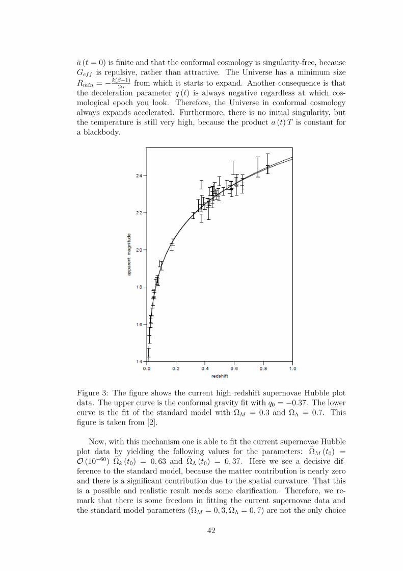
a (t = 0) is finite and that the conformal cosmology is singularity-free, becauseGeff is repulsive, rather than attractive. The Universe has a minimum sizeRmin = −k(β−1)

2α from which it starts to expand. Another consequence is thatthe deceleration parameter q (t) is always negative regardless at which cos-mological epoch you look. Therefore, the Universe in conformal cosmologyalways expands accelerated. Furthermore, there is no initial singularity, butthe temperature is still very high, because the product a (t)T is constant fora blackbody.

Figure 3: The figure shows the current high redshift supernovae Hubble plotdata. The upper curve is the conformal gravity fit with q0 = −0.37. The lowercurve is the fit of the standard model with ΩM = 0.3 and ΩΛ = 0.7. Thisfigure is taken from [2].

Now, with this mechanism one is able to fit the current supernovae Hubbleplot data by yielding the following values for the parameters: ΩM (t0) =O (10−60) Ωk (t0) = 0, 63 and ΩΛ (t0) = 0, 37. Here we see a decisive dif-ference to the standard model, because the matter contribution is nearly zeroand there is a significant contribution due to the spatial curvature. That thisis a possible and realistic result needs some clarification. Therefore, we re-mark that there is some freedom in fitting the current supernovae data andthe standard model parameters (ΩM = 0, 3,ΩΛ = 0, 7) are not the only choice

42

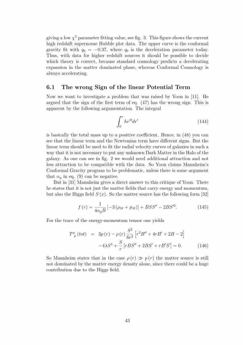
giving a low χ2 parameter fitting value, see fig. 3. This figure shows the currenthigh redshift supernovae Hubble plot data. The upper curve is the conformalgravity fit with q0 = −0.37, where q0 is the deceleration parameter today.Thus, with data for higher redshift sources it should be possible to decidewhich theory is correct, because standard cosmology predicts a deceleratingexpansion in the matter dominated phase, whereas Conformal Cosmology isalways accelerating.

6.1 The wrong Sign of the linear Potential TermNow we want to investigate a problem that was raised by Yoon in [11]. Heargued that the sign of the first term of eq. (47) has the wrong sign. This isapparent by the following argumentation. The integral

r

0hr′2dr′ (144)

is basically the total mass up to a positive coefficient. Hence, in (48) you cansee that the linear term and the Newtonian term have different signs. But thelinear term should be used to fit the radial velocity curves of galaxies in such away that it is not necessary to put any unknown Dark Matter in the Halo of thegalaxy. As one can see in fig. 2 we would need additional attraction and notless attraction to be compatible with the data. So Yoon claims Mannheim’sConformal Gravity program to be problematic, unless there is some argumentthat αg in eq. (9) can be negative.

But in [31] Mannheim gives a direct answer to this critique of Yoon. Therehe states that it is not just the matter fields that carry energy and momentum,but also the Higgs field S (x). So the matter source has the following form [32]

f (r) = 14αgB

[−3 (ρM + pM)] +BSS ′′ − 2BS ′2. (145)

For the trace of the energy-momentum tensor one yields

T µµ (tot) = 3p (r)− ρ (r) S2

6r2

[r2B′′ + 4rB′ + 2B − 2

]−4λS4 + S

r[rBS ′′ + 2BS ′ + rB′S ′] = 0. (146)

So Mannheim states that in the case ρ (r) p (r) the matter source is stillnot dominated by the matter energy density alone, since there could be a hugecontribution due to the Higgs field.

43

7 Wave Equation and its SolutionIn this thesis we presented several problems of the theory of General Relativ-ity and how Conformal Gravity may be able to solve these problems. Buta viable theory of gravity has to achieve more than the presented problemsabout Dark Matter, Dark Energy and Quantum Gravity. In subsection 2.1 wealready mentioned the measurements of binary systems like the Hulse-Taylorbinary. It was discovered by Russell Alan Hulse and Joseph Hooton Taylorof the University of Massachusetts Amherst. It is a gravitational bound sys-tem composed of the pulsar (PSR B1913+16) and another neutron star (PSRJ1915+1606) orbiting around a common center of mass. By their observationsHulse and Taylor have shown that the orbit of the binary system is contracting.This could possibly be the result of energy emission of the system. GeneralRelativity predicts such a energy emission due to gravitational waves. In fig. 4one can see the observed decay of the periastron (data points) and the predic-tion of General Relativity. This prediction seems to be perfectly in line withthe observation.

Figure 4: Orbital decay of PSR B1913+16. The data points show the observeddecay of the periastron in time. The solid line is the prediction of GeneralRelativity. This figure is taken from [33].

Thus, also Conformal Gravity has to contain a mechanism that explainsthe contraction of the orbit of the binary system. Therefore, in this chapterwe want to present the first steps to analyze classical gravitational waves andthe radiated power of such a system in Conformal Gravity.

44

7.1 Linearization of the Bach EquationTo analyze classical gravitational waves in Conformal Gravity one can proceedquite analogously to the mechanism in General Relativity.

Therefore, we can expand the metric around flat space-time

gµν = ηµν + hµν (147)

with |hµν | 1. hµν is called the metric perturbation which represents thegravitational wave. Now we have to insert (147) in the Bach equations (20)and keep just the terms linear in hµν . Hence, we give a list of linearizedquantities here,

Rµνρσ = 1

2(∂ν∂ρh

µσ + ∂µ∂σhνρ − ∂µ∂ρhνσ − ∂ν∂σhµρ

), (148)

Rµν = 12(∂ρ∂µh

ρν −hµν − ∂µ∂νh+ ∂ν∂ρh

ρµ

), (149)

R = ∂µ∂νhµν −h, (150)

with h = ηµνhµν denoting the trace of the metric perturbation. By insertingthis linearized quantities we yield the following expressions

13W

(1)µν = 2

3ηµν∂ρ∂σ hρσ − 2

3ηµν h−23∂µ∂ν∂ρ∂σh

ρσ + 23∂µ∂ν h,(151)

W (2)µν = 1

2ηµν∂ρ∂σ hρσ − 1

2ηµν h−12 hµν + 1

2∂µ∂ν h (152)

−∂µ∂ν∂σ∂ρhρσ + 12∂

ν∂σ hσµ + 1

2∂µ∂σ h

σν .

Finally, this gives

Wµν = W (2)µν −

13W

(1)µν = −1

6ηµν∂ρ∂σ hρσ + 1

6ηµν h−13∂µ∂ν∂ρ∂σh

ρσ (153)

−16∂µ∂ν h−

12 hµν + 1

2∂ν∂ρ hρµ + 1

2∂µ∂ρ hρν .

Now we introduce a new quantity which is the analog to the trace reversedmetric perturbation in the standard theory: hµν = hµν − 1

4ηµνh. By rewritingeq. (20) in terms of hµν we yield

14αg

Tµν = −16ηµν∂ρ∂σ h

ρσ − 13∂µ∂ν∂ρ∂σh

ρσ − 12∂µ∂ρ h

ρν (154)

−12 hµν + 1

2 ∂ν∂ρhρµ + 1

2∂µ∂ρ hρν .

Here we can see that only the traceless part hµν of the metric perturbationcontributes to the wave equation. As hµν is a symmetric tensor and traceless ithas only 9 degrees of freedom. Further, by choosing the Lorenz gauge ∂ν hµν = 0we are left with only five degrees of freedom. The result is a fourth-order waveequation

−12 hµν = 1

4αgTµν . (155)

45

In the vacuum case we see that the equation basically consists of the 2-operator applied to the metric perturbation hµν . So the solutions to the second-order wave equation

hµν = Cµνe±i(~k~x−ωt) (156)

trivially satisfy eq. (155), with ω = ±∣∣∣~k∣∣∣ and Cµνkµ = 0, Cµ

µ = 0.But a fourth-order equation has additional solutions. These solutions are

of the following typeCµν (n · x) e±i(~k~x−ωt), (157)

where n is a unit vector that obeys nµnµ = −1. This seems to be a problem,because this solution grows linearly in time, which could lead to energy conser-vation being violated. But although the vacuum solution in Conformal Gravityshows a quite different behavior this does not automatically lead to rule outthe theory of Conformal Gravity. So first let us have a look at gravitationalwaves in General Relativity.

The sources which lead to gravitational waves are far away from our grav-itational wave observatories. We know that gravitational waves decrease withthe distance to the source like r−1. But as spatial diameter of the detectorson earth are relatively small the amplitude of the wave does not change sig-nificantly over this distance. Therefore, we can approximate the gravitationalwaves as a plane wave hµνplane (x) = Cµνeikx in General Relativity.

In Conformal Gravity the vacuum solution actually grows in time or space.But this does not mean that this behavior has to be observable, since it isnot a priori clear that these modes are actually excited by any source thatradiates gravitational waves. Furthermore, even if the radiated waves werereally growing in time or space, it is still not clear that we are able to observethis, since it could be a coordinate artefact. Thus, it could be possible that bychoosing appropriate coordinates these growing solutions do not appear.

Another point is that a wave has to be produced at some specific pointof space-time and only after being excited the wave can start to grow. Butour detectors will always measure the same amplitude of the gravitationalwave. A possibility to measure differences to the standard gravitational wavesis to measure gravitational waves of systems which radiate gravitational waveswith the same amplitude, but with different distances to the earth or to by asequence of detectors along the path of the wave.

Consequently, to learn more about the behavior of gravitational waves inConformal Gravity we study the inhomogeneous wave equation in the nextsection.

7.2 Inhomogeneous Wave EquationIn this paragraph we want to investigate the solution to the inhomogeneouswave equation (155).

Of course the solutions to the inhomogeneous second-order wave equationare solutions to the inhomogeneous fourth-order wave equation. Thus, thestandard gravitational wave solutions are also present in Conformal Gravity.

46

But again we can find additional solutions. Let us make a simplified calcu-lation to get a basic understanding of the form of these additional solutions.Hence, we apply the d’Alembert operator to a radial propagating wave whichis constant in amplitude

ei(t−r) =(−∂2

t + ∂2r + 2

r∂r

)ei(t−r) = −2i

rei(t−r). (158)

The result is a radially propagating wave with an amplitude that decreases liker−1. So we know that this is a solution to the second-order Poisson equation.Thus, we can apply the d’Alembert operator to eq. (158) and we see thata constant spherical wave is a solution to the fourth-order Poisson equation.Let us note here that this is the solution to a very specific energy-momentumtensor T µνM and it is not clear whether this represents a physical system or not.

Now we continue with the general solution to (155) by making use of themethod of Green’s function. Let us write

hµν (x) = − 12αg

d4x′G (x− x′)Tµν (x′) , (159)

where x is the position 4-vector. The defining equation for the Green’s functionis

G (t− t′, ~x− ~x′) = δ (t− t′) δ (~x− ~x′) , (160)where we can set t′ = ~x′ = 0. We can reintroduce arbitrary t′, ~x′ in the endwithout loss of generality. We start with a Fourier transformation on the lefthand side of eq. (160) and apply the squared d’Alembert operator to theintegrand

1

(2π)4

dωd3ke(−i(ωt−~k~x))G

(ω,~k

)= δ (t) δ (~x) ,(161)

1(2π)4

dωd3k

(ω4 + ~k4 − 2ω2~k2

)e(−i(ωt−~k~x))G

(ω,~k

)= δ (t) δ (~x) .(162)

From (162) we can read off the Fourier transformation of the Green’s function

G(ω,~k

)= 1ω4 + ~k4 − 2ω2~k2

. (163)

Thus, we have to solve the following integral

G (t, ~x) = 1(2π)4

dωd3k

e(−i(ωt−~k~x))

ω4 + ~k4 − 2ω2~k2. (164)

At first let us execute the angular integration in spherical coordinates. Thisyields

G (t, ~x) = 2(2π)3 |~x|

∞−∞

dω

∞0

dkk sin (k |~x|)

ω4 + ~k4 − 2ω2~k2e(−iωt). (165)

47

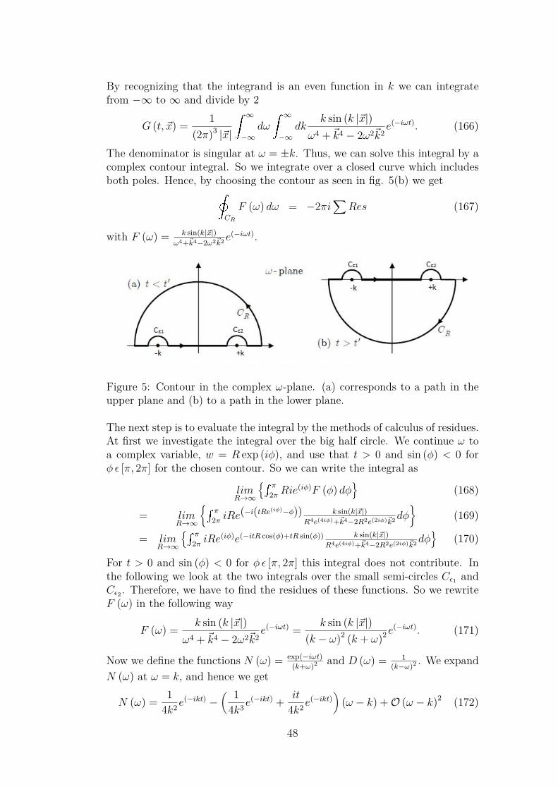
By recognizing that the integrand is an even function in k we can integratefrom −∞ to ∞ and divide by 2

G (t, ~x) = 1(2π)3 |~x|

∞−∞

dω

∞−∞

dkk sin (k |~x|)

ω4 + ~k4 − 2ω2~k2e(−iωt). (166)

The denominator is singular at ω = ±k. Thus, we can solve this integral by acomplex contour integral. So we integrate over a closed curve which includesboth poles. Hence, by choosing the contour as seen in fig. 5(b) we get

CR

F (ω) dω = −2πi∑

Res (167)

with F (ω) = k sin(k|~x|)ω4+~k4−2ω2~k2 e

(−iωt).

Figure 5: Contour in the complex ω-plane. (a) corresponds to a path in theupper plane and (b) to a path in the lower plane.

The next step is to evaluate the integral by the methods of calculus of residues.At first we investigate the integral over the big half circle. We continue ω toa complex variable, w = R exp (iφ), and use that t > 0 and sin (φ) < 0 forφ ε [π, 2π] for the chosen contour. So we can write the integral as

limR→∞

π2π Rie

(iφ)F (φ) dφ

(168)

= limR→∞

π2π iRe

(−i(tRe(iφ)−φ)) k sin(k|~x|)R4e(4iφ)+~k4−2R2e(2iφ)~k2dφ

(169)

= limR→∞

π2π iRe

(iφ)e(−itR cos(φ)+tR sin(φ)) k sin(k|~x|)R4e(4iφ)+~k4−2R2e(2iφ)~k2dφ

(170)

For t > 0 and sin (φ) < 0 for φ ε [π, 2π] this integral does not contribute. Inthe following we look at the two integrals over the small semi-circles Cε1 andCε2 . Therefore, we have to find the residues of these functions. So we rewriteF (ω) in the following way

F (ω) = k sin (k |~x|)ω4 + ~k4 − 2ω2~k2

e(−iωt) = k sin (k |~x|)(k − ω)2 (k + ω)2 e

(−iωt). (171)

Now we define the functions N (ω) = exp(−iωt)(k+ω)2 and D (ω) = 1

(k−ω)2 . We expandN (ω) at ω = k, and hence we get

N (ω) = 14k2 e

(−ikt) −( 1

4k3 e(−ikt) + it

4k2 e(−ikt)

)(ω − k) +O (ω − k)2 (172)

48

and

N (ω)D (ω) =e(−ikt)

4k2 −(e(−ikt)

4k3 + ite(−ikt)

4k2

)(ω − k) +O (ω − k)2

(ω − k)2 (173)

So the residuum is

Res+k =( 1

4k3 e(−ikt) + it

4k2 e(−ikt)

)= e(−ikt) (1 + ikt)

4k3 . (174)

In analogy to this calculation we get

Res−k = e(ikt) (−1 + ikt)4k3 . (175)

If we combine the remaining integrals, they give a Cauchy principal valueintegral. So this is the integral we want to evaluate

limR→∞

R

−RdωF (ω) = −1

2πie(ikt) (−1 + ikt) sin (k |~x|)

k2 (176)

+e(−ikt) (1 + ikt) sin (k |~x|)k2

Θ (t) .

Then we insert this result in (166) and get the following remaining integral

G (t, ~x) = Θ (t)32π2 |~x|

∞−∞

dk

(1− ikt)

k2

[e(ik(t+|~x|)) − e(ik(t−|~x|))

](177)

−(1 + ikt)k2

[e(−ik(t−|~x|)) − e(−ik(t+|~x|))

].

The next step is to execute the k-integral. Therefore, we bring the integral inthe following form and notice that this integral is non-singular

G (t, ~x) = Θ (t)16π2 |~x|

∞−∞

dk1k2 [− cos (k (|~x| − t)) + kt sin (k (|~x| − t)) (178)

+ cos (k (|~x|+ t)) + kt sin (k (|~x|+ t))] .

This can be integrated and yields

G (t, ~x) = −Θ (t)16π

(|~x| (|t− |~x|| − |t+ |~x||) + t (|t− |~x||+ |t+ |~x||))t2 − ~x2 . (179)

Now this equation can be solved for the cases t > |~x|, t < |~x|, t = |~x|. In thefirst case we get

G (t, ~x) = − 18πΘ (t− t′) Θ

[(t− t′)−

∣∣∣~x− ~x′∣∣∣] . (180)

49

In the second case the whole term gives just zero. The limit t→ |~x| does notexist, because the limits from the left and the right do not coincide. Thus,after reintroducing t→ t− t′ and |~x| →

∣∣∣~x− ~x′∣∣∣, we get for the Green function

G (t− t′, ~x− ~x′) = − 18πΘ (t− t′) Θ

[(t− t′)−

∣∣∣~x− ~x′∣∣∣] . (181)

Now we can insert the Green function into eq. (159) and yield

hµν (x) = 116παg

d4x′Θ (t− t′) Θ

[(t− t′)−

∣∣∣~x− ~x′∣∣∣]Tµν (x′) . (182)

It is quite remarkable that there is a constant Green’s function for thepast light cone and everywhere else it is zero. One would intuitively expectthat there has to be some retardation in the solution in order to have a wavesolution, which travels at the speed of light. Furthermore, it seems that therecould be a problem with the energy conservation too, because the wave doesnot decrease with growing distance. But in Conformal Gravity one does nothave the same energy-momentum tensor as in General Relativity. Hence, tounderstand more about these issues one has to investigate the energy contentof such a wave and how it couples to matter.

50

8 Summary and OutlookIn this thesis we presented an overview of the theory of Conformal Gravity.In chapter 2 we started with the fundamental principles of the standard form-alism for gravity given by General Relativity. Thus, we figured out whichproperties of General Relativity are necessary for a viable theory gravity andshould be kept. Taking this into account we introduced Conformal Gravitywith its underlying Weyl symmetry. We found the equation of motion for thegravitational field, the Bach equations, which replace the well-known Einsteinequations. After that we turned to the Dark Matter problem in chapter 3.General Relativity has to invoke some kind of unknown Dark Matter to makecorrect predictions about the velocities of stars and gas in galactic rotationcurves. Conformal Gravity can solve this problem without Dark Matter. Anadditional attractive term in the non-relativistic weak field limit makes DarkMatter redundant. In chapter 4 we turned to the microscopic description ofConformal Gravity. We pointed out that Conformal Gravity and especiallythe Bach equations have to be treated quantum-mechanically on a funda-mental level. Additionally, we had a brief look on how the gravitational fieldis quantized in Conformal Gravity and how this could solve the zero-pointenergy problem that occurs in the standard formalism. Remarkable aboutConformal Gravity is that the gravitational field is not quantized by its own,but by the coupling to the particle matter fields. Another important issue isthe generation of masses in chapter 5. In principle mass terms are forbidden onthe level of the lagrange density and thus, quite analogously to the StandardModel of particle physics, masses have to be generated by dynamical Higgsmechanism. Chapter 6 gives a short introduction to the non-perturbative cos-mology in Conformal Gravity. Here we saw that one ends up with the sameform for the evolution equation for the Universe, the Friedmann equation,but quite remarkably the gravitational coupling constant acts repulsive ratherthan attractive. Nevertheless, with conformal cosmology one is able to fit thecurrent high redshift supernovae Hubble plot data. In chapter 7 we dealt withclassical gravitational waves in Conformal Gravity. Here we calculated theGreen’s function for the wave equation in Conformal Gravity to first order inperturbation theory. Noteworthy, the modes we have found do not show theusual properties of waves like a decreasing amplitude with a growing distance.Furthermore, these modes do not necessarily travel with the speed of light.

By this summary we see that Conformal Gravity tackles the main prob-lems of the standard theory of gravity and possibly is able to solve them. Butstill there are several concerns. One of the biggest concerns was that usuallytheories of higher than second order derivatives are believed to consist ghosts.That means that there are states of negative energy or negative norm. Thus,Conformal Gravity was supposed to be a non-unitary theory. But in sev-eral publications [3, 34, 35] Mannheim and Bender showed that a hermitianHamilton operator is sufficient to have real eigenstates, but in fact also PT -symmetric Hamilton operators yield real eigenstates. In consequence, theywere able to show that the evolution of quantum states in Conformal Gravity

51

is unitary.But still there are a lot of open questions and tasks in proving that Con-

formal Gravity is a viable theory of gravity. As was already mentioned inchapter 3 it is not clear that Conformal Gravity is able to explain phenomenalike the Bullet cluster or the gravitational lensing of galaxy clusters. Especially,it could be important to include the cosmological −κR term in (91). Besidesthat, one has to investigate whether Conformal Gravity is able to describethe anisotropies of the cosmic microwave background as exact as the standardtheory of cosmology. Furthermore, there is not very much progress in devel-oping the theory of cosmological perturbations δM and structure growth, yet.A priori in Conformal Gravity it seems that it is quite hard to explain howcosmological inhomogeneities can grow up to the non-linear regime of δM ∼ 1fast enough without any Dark Matter. First steps towards addressing theseproblems are given in [36, 37].

Extraordinarily, conformal cosmology provides a test for Conformal Grav-ity by redshift measurements above z ∼ 1. If these measurements find adecelerating expansion of the Universe, this immediately falsifies the theory ofConformal Gravity, because in Conformal Gravity the Universe is acceleratingin all epochs.

Lastly, also the decreasing orbits of binary pulsars bears data to test Con-formal Gravity. In chapter 7 we presented first steps for calculating gravita-tional waves in Conformal Gravity. Although this is still work in progress, onerecognizes that these gravitational waves have a different structure comparedto them in General Relativity. Therefore, the next step is to investigate theradiated energy by these waves to see whether energy conservation is violatedor not. On top of that, the Advanced Ligo experiment announced to be ableto measure gravitational waves radiated by binary systems in the near future.Thus, it would be possible to decide which theory provides the correct formfor gravitational waves.

As a conclusion we can say that Conformal Gravity holds some remarkableproperties. It is able to explain several striking problems of theoretical physicsin an excellent way. But nevertheless, Conformal Gravity has some weaknessesthat have to be investigated in more detail. And furthermore, there is a hugebunch of unsolved tasks, especially for cosmology. To sum up, one can statethat it is indeed reasonable as well necessary to put further investigation inthe theory of Conformal Gravity as long as there is no detection of any kindof Dark Matter and Dark Energy which would solve the problems of GeneralRelativity.

52

References[1] P.D. Mannheim, Making the Case for Conformal Gravity, ArXiv:

1101.2186v2 [hep-th], 2011

[2] P.D. Mannheim, Alternatives to Dark Matter and Dark Energy, Prog.Part. Nucl. Phys. 56 (2) 340, 2006

[3] P.D. Mannheim, Comprehensive solution to the cosmological constant,zero-point, and quantum gravity problems, arXiv:0909.0212v5 [hep-th],2010

[4] C.W. Misner, K.S. Thorne, J.A. Wheeler, Gravitation, W. H. Freemanand Company, San Francico, 1973

[5] C. Lanczos, A remarkable property of the Riemann-Christoffel tensor infour dimensions, Anns. Math., Vol. 39, No. 4, 842, 1938

[6] P.D. Mannheim, D. Kazanas, Newtonian limit of Conformal Gravity andthe lack of necessity of the second order poisson equation, Gen. Rel. Grav.,Vol. 26, No. 4, 1994

[7] S.M. Carroll, The cosmological constant, arXiv:0004075v2 [astro-ph], 2000

[8] P.D. Mannheim, D. Kazanas, Exact vacuum solution to Conformal WeylGravity and galactic rotation curves, Astrophys. J., 342, 635, 1988

[9] D. Kazanas, P.D. Mannheim, General structure of the equations of motionin Conformal Weyl Gravity, Astrophys. 76:431-453, 1991

[10] P.D. Mannheim, J.G. O’Brien, Impact of a global quadratic potential ongalactic rotation curves, Phys. Rev. Lett. 106 121101, 2011

[11] Y. Yoon, Problems with Mannheim’s conformal gravity program, Phys.Rev. D 88, 027504, 2013

[12] C.M. Will, The Confrontation between General Relativity and Experi-ment, Living Rev. Relativity, 9, 3, 2006

[13] P.J. Mohr, B.N. Taylor, D.B. Newell, CODATA recommended values ofthe fundamental physical constants: 2010, Rev. of mod. Phys., 84, 2012

[14] Richard P. Feynman, The Feynman Lectures on Physics, Mainly Mech-anics, Radiation and Heat (Volume 1), Addison-Wesley Publishing Com-pany, sixth printing, Reading, Massachusetts, 1977

[15] K.G. Begeman, Ph. D. Dissertation, Rijksuniversiteit Groningen, 1987

[16] K.G. Begeman, H I rotation curves of spiral galaxies. I - NGC 3198,Astronomy and Astrophysics, 223, 47, 1989

53

[17] D. S. Gorbunov, V.A. Rubakov, Introduction to the theory of the earlyuniverse, Hot Big Bang Theory, World Scientific Publishing Co. Pte. Ltd.,Singapore, 2011

[18] P.D. Mannheim, Linear Potentials and Galactic Rotation Curves - Form-alism, ArXiv: 9307004v1 astro-ph, 1993

[19] P.D. Mannheim, J.G. O’Brien, Fitting galactic rotation curves with con-formal gravity and a global quadratic potential, arXiv:1011.3495v4 astro-ph.CO, 2012

[20] P.D. Mannheim, Are galactic rotation curves really flat?, Astrophys. J.479, 659, 1996

[21] R.B. Tully, J.R. Fisher, A new method of determining distances to galax-ies, A&A, 54, 661, 1977

[22] K.C. Freeman, On the Disks of Spiral and S0 Galaxies, Astrophys. J.,160, 1970

[23] M. Milgrom, Dynamics with a non-standard inertia-acceleration relation:an alternative to dark matter, Ann. Phys. 229, 384-415, 1994

[24] P.D. Mannheim, J.G. O’Brien, Galactic rotation curves in conformal grav-ity, ArXiv: 1211.0188v1 [astro-ph.CO], 2012

[25] D. S. Gorbunov, V.A. Rubakov, Introduction to the theory of the earlyuniverse, Cosmological Perturbations and inflationary theory, World Sci-entific Publishing Co. Pte. Ltd., Singapore, 2011

[26] D. Clowe, M. Bradac, A. H. Gonzalez, M. Markevitch, S. W. Randall, C.Jones and D. Zaritsky, A direct empirical proof of the existence of DarkMatter, Astrophys. J. 648, L109, [arXiv:astro-ph/0608407], 2006

[27] P.D. Mannheim, Intrinsically quantum-mechanical gravity and the cos-mological constant problem, arXiv:1005.5108v4 [hep-th], 2011

[28] P.D. Mannheim, Living without Supersymmetry - the conformal altern-ative and a dynamical Higgs boson, arXiv:1506.01399v2 [hep-ph], 2015

[29] P.D. Mannheim, Dynamical mass and geodesic motion, Gen. Rel. Grav.,Vol. 25, 7, 1993

[30] P.D. Mannheim, Conformal Gravity and the Flatness Problem, Astro-phys. 391:429-432, 1992

[31] P.D. Mannheim, Critique of ’Problem’s with Mannheim’s conformal grav-ity program’ by Yoon, arXiv:1506.02479.v1 [gr-qc], 2015

[32] P.D. Mannheim, Schwarzschild limit of conformal gravity in the presenceof macroscopic scalar field, arXiv:0703037v1 [gr-qc], 2007

54

[33] J.M. Weisberg, J.H. Taylor, Relativistic Binary Pulsar B1913+16: ThirtyYears of Observations and Analysis, arXiv:0407149.v1 [astro-ph], 2004

[34] C.M. Bender, P.D. Mannheim, Exactly solvable PT-symmetric Hamilto-nian having no Hermitian counterpart, phys. rev. D 78, 025022, 2008

[35] P.D. Mannheim, PT symmetry as a necessary and sufficient condition forunitary time evolution, arXiv:0912.2635.v3 [hep-th], 2012

[36] P.D. Mannheim, Cosmological perturbations in conformal gravity,arXiv:1109.4119 [gr-qc], 2012

[37] P. Mezgolits, D. Grumiller, Cosmological perturbations in a conformalgravity based model, 2015

55

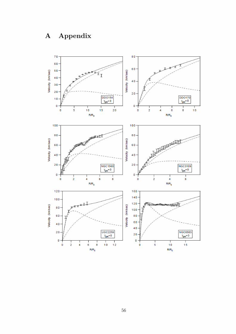
A Appendix

56

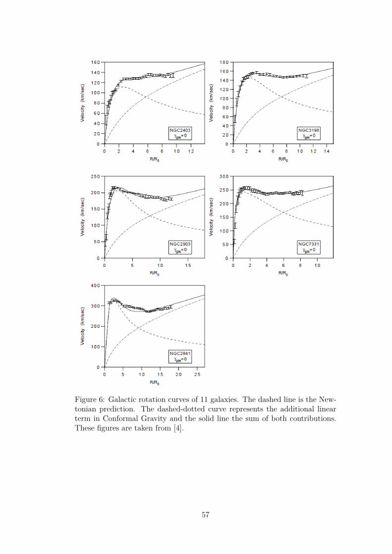
Figure 6: Galactic rotation curves of 11 galaxies. The dashed line is the New-tonian prediction. The dashed-dotted curve represents the additional linearterm in Conformal Gravity and the solid line the sum of both contributions.These figures are taken from [4].

57

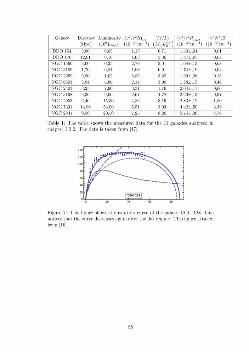
Galaxy Distance(Mpc)

Luminosity(109LB

) (v2/c2R

)tot(

10−30cm−1) (M/L)(ML

−1B

) (v2/c2R

)net(

10−30cm−1) γ∗N∗/2(10−30cm−1)

DDO 154 3,80 0,05 1,15 0,71 1,49±,04 0,01DDO 170 12,01 0,16 1,63 5,36 1,47±,07 0,04NGC 1560 3,00 0,35 2,70 2,01 1,68±,13 0,08NGC 3109 1,70 0,81 1,98 0,01 1,74±,19 0,03UGC 2259 9,80 1,02 3,85 3,62 1,99±,26 0,15NGC 6503 5,94 4,80 2,14 3,00 1,58±,15 0,46NGC 2403 3,25 7,90 3,31 1,76 2,04±,17 0,66NGC 3198 9,36 9,00 2,67 4,78 2,23±,13 0,97NGC 2903 6,40 15,30 4,86 3,15 2,83±,19 1,80NGC 7331 14,90 54,00 5,51 3,03 4,42±,50 3,39NGC 2841 9,50 20,50 7,25 8,26 5,75±,30 4,76

Table 1: The table shows the measured data for the 11 galaxies analyzed inchapter 3.3.2. The data is taken from [17].

Figure 7: This figure shows the rotation curve of the galaxy UGC 128. Onenotices that the curve decreases again after the flat regime. This figure is takenfrom [16].

58