path planning for unmanned underwater vehicle in … · the optimal path is converted to desirable...

1054

Abstract In this research, generation of a short and smooth path in three-dimen-sional space with obstacles for guiding an Unmanned Underwater Vehi-cle (UUV) without collision is investigated. This is done by utilizing spline technique, in which the spline control points positions are deter-mined by Imperialist Competitive Algorithm (ICA) in three-dimensional space such that the shortest possible path from the starting point to the target point without colliding with obstacles is achieved. Furthermore, for guiding the UUV in the generated path, an Interval Type-2 Fuzzy Logic Controller (IT2FLC), the coefficients of which are optimized by considering an objective function that includes quadratic terms of the input forces and state error of the system, is used. Selecting such objec-tive function reduces the control error and also the force applied to the UUV, which consequently leads to reduction of energy consumption. Therefore, by using a special method, desired signals of UUV state are obtained from generated three-dimensional optimal path such that tracking these signals by the controller leads to the tracking of this path by UUV. In this paper, the dynamical model of the UUV, entitled as “mUUV-WJ-1”, is derived and its hydrodynamic coefficients are calcu-lated by CFD in order to be used in the simulations. For simulation by the method presented in this study, three environments with different obstacles are intended in order to check the performance of the IT2FLC controller in generating optimal paths for guiding the UUV. In this ar-ticle, in addition to ICA, Particle Swarm Optimization (PSO) and Arti-ficial Bee Colony (ABC) are also used for generation of the paths and the results are compared with each other. The results show the appro-priate performance of ICA rather than ABC and PSO. Moreover, to evaluate the performance of the IT2FLC, optimal Type-1 Fuzzy Logic Controller (T1FLC) and Proportional Integrator Differentiator (PID) controller are designed and applied to the UUV and compared with each other. The simulation results show the superiority of the IT2FLC than the other two controllers. Keywords Path Planning; Spline; ICA; Optimal IT2FLC; UUV; Nelder-Mead algorithm.

Path Planning for Unmanned Underwater Vehicle in 3D Space with Obstacles Using Spline-Imperialist Competitive Algorithm and Optimal Interval Type-2 Fuzzy Logic Controller

Ehsan Zakeri a *

Said Farahat b

Seyed Alireza Moezi c

Amin Zare d

a Young Researchers and Elite Club, Shiraz Branch, Islamic Azad University, Shiraz, Iran; [email protected]. b Department of Mechanical Engineering, University of Sistan and Baluchestan, Zahedan, Iran; [email protected]. c Young Researchers and Elite Club, Shiraz Branch, Islamic Azad University, Shiraz, Iran; [email protected]. d Young Researchers and Elite Club, Shiraz Branch, Islamic Azad University, Shiraz, Iran; [email protected]. * Corresponding Author http://dx.doi.org/10.1590/1679-78252029

Received 08.04.2015 In revised form 13.02.2016 Accepted 19.02.2016 Available online 27.02.2016

E. Zakeri et al. / Path Planning for Unmanned Underwater Vehicle in 3D Space with Obstacles Using Spline-Imperialist... 1055

Latin American Journal of Solids and Structures 13 (2016) 1054-1085

1 INTRODUCTION

The Unmanned Underwater Vehicles (UUVs) have many components that generally include mechani-cal, automatic controllers design and optimal path planning sections. Generating the optimal path is one of the main issues of UUVs and has attracted many researchers and scientists and lots of researches have been done on it. In this field, an algorithm for path planning based on fuzzy logic for Autonomous Underwater Vehicles (AUVs) in unknown three-dimensional space is provided by Liu et al. (2012). In this algorithm, the problem of three-dimensional path planning is decomposed to two independent plan-ning problems in horizontal and vertical planes. In this way, avoiding collision with obstacles and finding the target in each plane takes place individually. In another study, in order to generate the UUV path in the horizontal plane, a new method based on quad tree and modified ant colony optimization algo-rithm, in which the horizontal plane is modeled using quad tree, was proposed by Guang-Lei and He-Ming (2012). An autonomous method for path planning of a UUV of six degrees of freedom (DOF) was proposed by Poppinga et al. (2011) based on Rapidly-exploring Random Trees (RRT) and probabilistic roadmap method. Path planning for AUV in a dynamic environment by using fuzzy control-Particle Swarm Optimization (PSO) was provided by Zhu et al. (2011) in which the fuzzy controller was devel-oped to create a collision-free path from the starting point to the target point. PSO was utilized to obtain the parameters of fuzzy controller. A multi-objective path planning was presented for vehicles by Ahmed and Deb (2013), in which the length, safety and smoothness of the path were the objectives of the optimization. Furthermore, the non-dominant sorting method of elitist genetic algorithm was used for optimization. In another research, Mashadi and Majidi (2014) have proposed the global optimal path planning of an autonomous vehicle for overtaking a moving obstacle, by performing a double lane-change maneuver after detecting it in a proper distance ahead. Ali et al. (2015) has proposed a method to prevent the underwater robots from colliding with obstacles. In this method, they used type-2 fuzzy and ontology-based semantic knowledge for simulation, identifying obstacles and avoiding collisions. They also presented a simulator software for the use of other researchers in order to prevent collisions with obstacles, which reduced the cost and lack of need for practical tests. An important issue that any UUV should benefit from in its way passing from starting point to target point is avoiding obstacles and also planning a short path to the target. In this study, this is considered as the goal in generating the path. Moreover, smoothness of the generated path is another feature considered in this method. Therefore, in order to generate a path from the starting point to the target point in 3D space, at first some points are selected in 3D space in a given interval, then the starting and target points are consid-ered as the first and last points of the set of points on the path, respectively, and finally a curve is passed through these points by using the spline method. The position of these points should be selected in such a way that the final generated path does not collide with the obstacles in the environment. As in this case, the problem is converted to a constrained optimization problem.

In this study, in order to ensure accomplishing the answer, selection of spline control points is performed by using Imperialist Competitive Algorithm (ICA) (Atashpaz-Gargari and Lucas, 2007). This algorithm, which was spired by the competition of colonizing countries on the other colonial countries, doesn’t trap in local minima regarding its multiple search for the optimal answers, and due to this point it is used as a powerful tool for solving optimization problems in engineering problems (Hosseini-Moghari, 2015; Masoumi, 2015).

1056 E. Zakeri et al. / Path Planning for Unmanned Underwater Vehicle in 3D Space with Obstacles Using Spline-Imperialist...


After generating the optimal path, an appropriate controller is needed to guide the unmanned vehicle on the path. Selecting a suitable controller is of utmost importance, due to the remote control nature of unmanned vehicles (Zakeri et al., 2015; Zare et al., 2014) or robots (Zakeri et al., 2012; Zakeri et al., 2013; Zakeri et al 2014; Moezi et al., 2014). So far, researchers have presented different control methods for UUVs, including, control of a high-speed underwater robot using H∞ controller

(Zhang et al., 2015) or control of an underwater robot using dynamic sliding mode controller (Xu et al., 2015). Among various controllers, the fuzzy controller, due to its nonlinear structure and also no need of the dynamic model of the system in its design, has been used a lot (Moezi et al., 2014; Moezi et al. 2016) therefore, it has been used in much researches for controlling underwater vehicles, includ-ing, control of six DOF of an ROV or depth control of submarine robot using fuzzy controller (Ishaque, et al., 2010; Nag et al., 2013).

According to mentioned points, in this research, the optimal Interval Type-2 Fuzzy Logic Con-troller (IT2FLC) is considered in order to guide the UUV in the optimal path, because it is more robust against uncertainties, compared to Type-1 Fuzzy Logic Controller (T1FLC), due to the exist-ence of uncertainties in its Membership Functions (MFs) (Wu and Wan, 2006). In addition, since this controller has more parameters, a better choice is achieved in optimization; in other words, it is more flexible (Fayek, 2014). To optimize the parameters of this controller, Simplex Nelder-Mead optimiza-tion method has been used, due to its reasonable speed and accuracy (Nelder and Mead, 1965). In addition, as far as we know, optimzal IT2FLC hasn’t been applied on a UUV and not studied com-paratively yet. This could be due to the fact that this controller is new; because using IT2FLC as a controller has been popular during the past decade (Mendel, 2009). Therefore, utilizing this controller in this study can be a test of its performance on such systems.

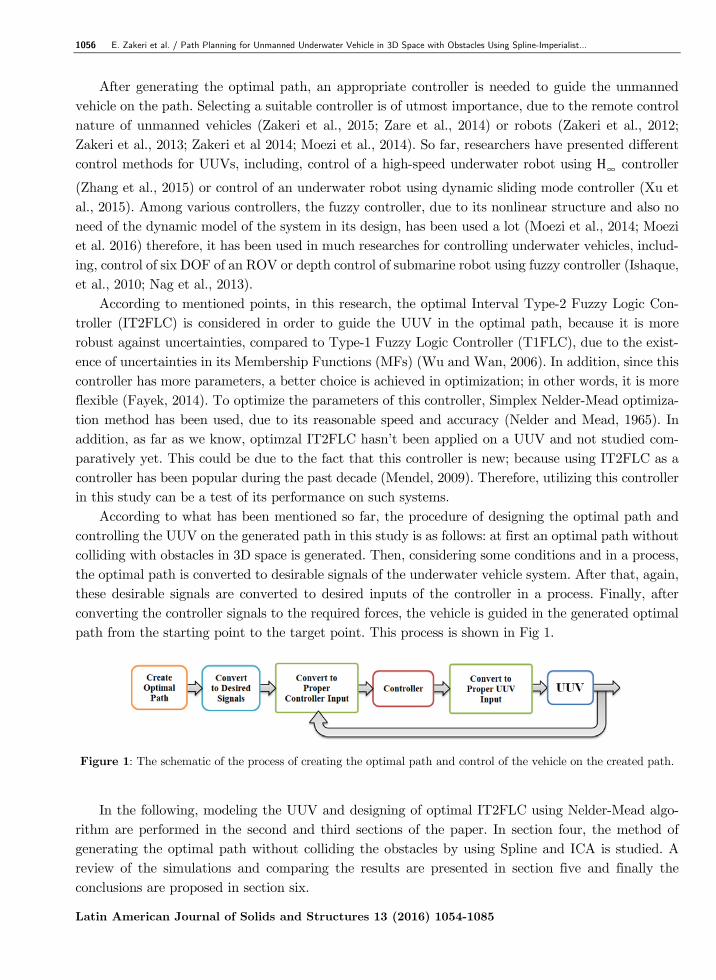
According to what has been mentioned so far, the procedure of designing the optimal path and controlling the UUV on the generated path in this study is as follows: at first an optimal path without colliding with obstacles in 3D space is generated. Then, considering some conditions and in a process, the optimal path is converted to desirable signals of the underwater vehicle system. After that, again, these desirable signals are converted to desired inputs of the controller in a process. Finally, after converting the controller signals to the required forces, the vehicle is guided in the generated optimal path from the starting point to the target point. This process is shown in Fig 1.

Figure 1: The schematic of the process of creating the optimal path and control of the vehicle on the created path.

In the following, modeling the UUV and designing of optimal IT2FLC using Nelder-Mead algo-

rithm are performed in the second and third sections of the paper. In section four, the method of generating the optimal path without colliding the obstacles by using Spline and ICA is studied. A review of the simulations and comparing the results are presented in section five and finally the conclusions are proposed in section six.



2 MODELING THE 6-DOF UUV

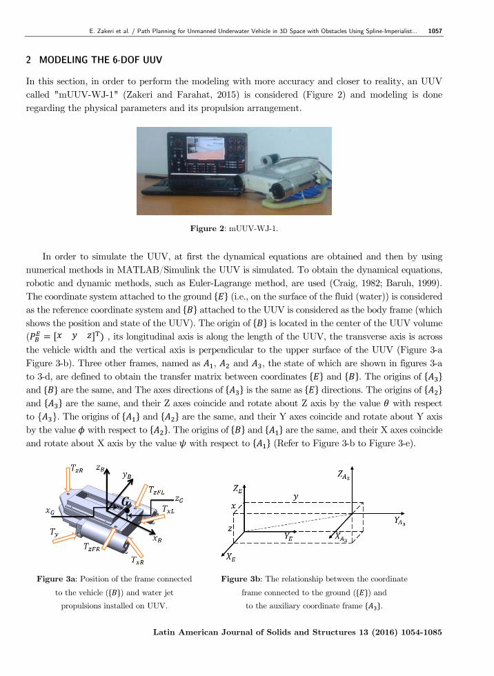
In this section, in order to perform the modeling with more accuracy and closer to reality, an UUV called "mUUV-WJ-1" (Zakeri and Farahat, 2015) is considered (Figure 2) and modeling is done regarding the physical parameters and its propulsion arrangement.

Figure 2: mUUV-WJ-1.

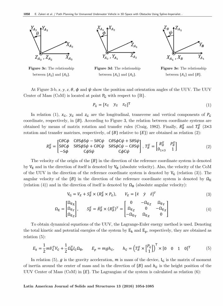
In order to simulate the UUV, at first the dynamical equations are obtained and then by using numerical methods in MATLAB/Simulink the UUV is simulated. To obtain the dynamical equations, robotic and dynamic methods, such as Euler-Lagrange method, are used (Craig, 1982; Baruh, 1999). The coordinate system attached to the ground (i.e., on the surface of the fluid (water)) is considered as the reference coordinate system and attached to the UUV is considered as the body frame (which shows the position and state of the UUV). The origin of is located in the center of the UUV volume ( , its longitudinal axis is along the length of the UUV, the transverse axis is across the vehicle width and the vertical axis is perpendicular to the upper surface of the UUV (Figure 3-a Figure 3-b). Three other frames, named as , and , the state of which are shown in figures 3-a to 3-d, are defined to obtain the transfer matrix between coordinates and . The origins of and are the same, and The axes directions of is the same as directions. The origins of and are the same, and their Z axes coincide and rotate about Z axis by the value with respect to { }. The origins of and are the same, and their Y axes coincide and rotate about Y axis by the value with respect to . The origins of and are the same, and their X axes coincide and rotate about X axis by the value with respect to (Refer to Figure 3-b to Figure 3-e).

Figure 3a: Position of the frame connected

to the vehicle ( ) and water jet

propulsions installed on UUV.

Figure 3b: The relationship between the coordinate

frame connected to the ground ( ) and

to the auxiliary coordinate frame .



Figure 3c: The relationship

between and .

Figure 3d: The relationship

between and .

Figure 3e: The relationship

between and .

At Figure 3-b, , , , , and show the position and orientation angles of the UUV. The UUV

Center of Mass (CoM) is located at point P with respect to {B}.

(1)

In relation (1), , and are the longitudinal, transverse and vertical components of coordinate, respectively, in . According to Figure 3, the relation between coordinate systems are obtained by means of matrix rotation and transfer rules (Craig, 1982). Finally, and (3 3 rotation and transfer matrixes, respectively, of relative to ) are obtained as relation (2):

C C C S S S C C S C S SS C S S S C C S S C C SS C S C C

, 0 1

(2)

The velocity of the origin of the in the direction of the reference coordinate system is denoted by V and in the direction of itself is denoted by V (absolute velocity). Also, the velocity of the CoM of the UUV in the direction of the reference coordinate system is denoted by V (relation (3)). The angular velocity of the in the direction of the reference coordinate system is denoted by Ω (relation (4)) and in the direction of itself is denoted by Ω (absolute angular velocity):

V , (3)

Ω

ΩΩΩ

,

0 Ω ΩΩ 0 ΩΩ Ω 0

(4)

To obtain dynamical equations of the UUV, the Lagrange-Euler energy method is used. Denoting the total kinetic and potential energies of the system by E and E , respectively, they are obtained as

relation (5):

12

12Ω Ω , ,

10 0 1 0 (5)

In relation (5), is the gravity acceleration, is mass of the device, I is the matrix of moment of inertia around the center of mass and in the direction of and is the height position of the UUV Center of Mass (CoM) in . The Lagrangian of the system is calculated as relation (6):



, , , (6)

In the relation (6), is the lagrangian of the system, is a vector of generalized coordinate and is a vector of generalized forces, which are obtained by calculating the virtual works of the hydro-

dynamic and propulsive forces and torques. In the following, the procedure of obtaining the general-ized forces ( ) is explained. External forces acting on the UUV, ignoring the gravity, include (In-zartsev, 2008):

Forces due to propulsion (system input). Hydrodynamic forces exerted on the vehicle. Archimedean force due to the weight of the displaced fluid.

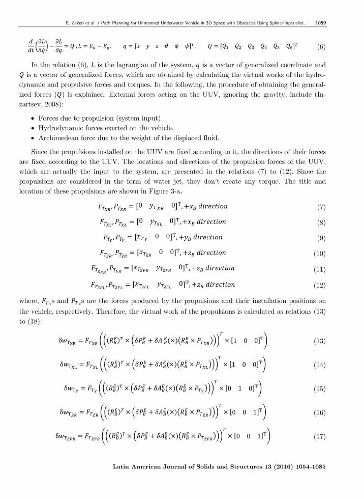
Since the propulsions installed on the UUV are fixed according to it, the directions of their forces are fixed according to the UUV. The locations and directions of the propulsion forces of the UUV, which are actually the input to the system, are presented in the relations (7) to (12). Since the propulsions are considered in the form of water jet, they don’t create any torque. The title and location of these propulsions are shown in Figure 3-a.

, 0 0 , (7)

, 0 0 , (8)

, 0 0 , (9)

, 0 0 , (10)

, 0 , (11)

, 0 , (12)

where, ∗s and ∗s are the forces produced by the propulsions and their installation positions on

the vehicle, respectively. Therefore, the virtual work of the propulsions is calculated as relations (13) to (18):

δ 1 0 0 (13)

δ 1 0 0 (14)

δ 0 1 0 (15)

δ 0 0 1 (16)

δ 0 0 1 (17)



δ 0 0 1 (18)

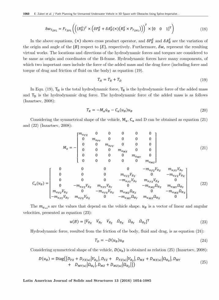
In the above equations, shows cross product operator, and and are the variation of the origin and angle of the respect to , respectively. Furthermore, ∗ represent the resulting virtual works. The locations and directions of the hydrodynamic forces and torques are considered to be same as origin and coordinates of the B-frame. Hydrodynamic forces have many components, of which two important ones include the force of the added mass and the drag force (including force and torque of drag and friction of fluid on the body) as equation (19).

(19)

In Equ. (19), T is the total hydrodynamic force, T is the hydrodynamic force of the added mass and T is the hydrodynamic drag force. The hydrodynamic force of the added mass is as follows (Inzartsev, 2008):

(20)

Considering the symmetrical shape of the vehicle, M , C and D can be obtained as equation (21) and (22) (Inzartsev, 2008):

0 0 0 0 00 0 0 0 00 0 0 0 00 0 0 0 00 0 0 0 00 0 0 0 0

(21)

0 0 0 00 0 0 00 0 0 00 0 Ω Ω

0 Ω 0 Ω0 Ω Ω 0

(22)

The ∗∗s are the values that depend on the vehicle shape. is a vector of linear and angular

velocities, presented as equation (23):

(23)

Hydrodynamic force, resulted from the friction of the body, fluid and drag, is as equation (24):

(24)

Considering symmetrical shape of the vehicle, is obtained as relation (25) (Inzartsev, 2008):

Diag | | , | | , | | Ω ,

| | Ω , | | Ω (25)



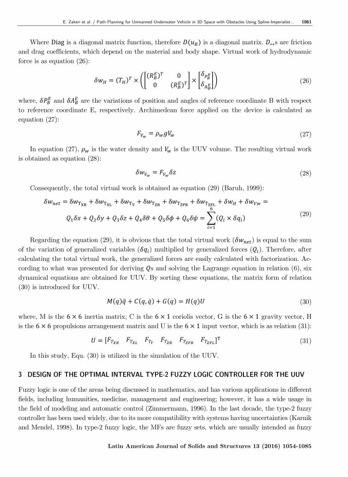
Where Diag is a diagonal matrix function, therefore is a diagonal matrix. ∗∗s are friction and drag coefficients, which depend on the material and body shape. Virtual work of hydrodynamic force is as equation (26):

00

(26)

where, and are the variations of position and angles of reference coordinate B with respect to reference coordinate E, respectively. Archimedean force applied on the device is calculated as equation (27):

(27)

In equation (27), is the water density and is the UUV volume. The resulting virtual work is obtained as equation (28):

(28)

Consequently, the total virtual work is obtained as equation (29) (Baruh, 1999):

δ δ δ δ δ δ

(29)

Regarding the equation (29), it is obvious that the total virtual work ( ) is equal to the sum of the variation of generalized variables ( ) multiplied by generalized forces ( ). Therefore, after calculating the total virtual work, the generalized forces are easily calculated with factorization. Ac-cording to what was presented for deriving s and solving the Lagrange equation in relation (6), six dynamical equations are obtained for UUV. By sorting these equations, the matrix form of relation (30) is introduced for UUV.

, (30)

where, M is the 6 6 inertia matrix, C is the 6 1 coriolis vector, G is the 6 1 gravity vector, H is the 6 6 propulsions arrangement matrix and U is the 6 1 input vector, which is as relation (31):

(31)

In this study, Equ. (30) is utilized in the simulation of the UUV. 3 DESIGN OF THE OPTIMAL INTERVAL TYPE-2 FUZZY LOGIC CONTROLLER FOR THE UUV

Fuzzy logic is one of the areas being discussed in mathematics, and has various applications in different fields, including humanities, medicine, management and engineering; however, it has a wide usage in the field of modeling and automatic control (Zimmermann, 1996). In the last decade, the type-2 fuzzy controller has been used widely, due to its more compatibility with systems having uncertainties (Karnik and Mendel, 1998). In type-2 fuzzy logic, the MFs are fuzzy sets, which are usually intended as fuzzy



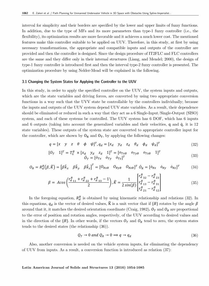
interval for simplicity and their borders are specified by the lower and upper limits of fuzzy functions. In addition, due to the type of MFs and its more parameters than type-1 fuzzy controller (i.e., the flexibility), its optimization results are more favorable and it achieves a much lower cost. The mentioned features make this controller suitable to be applied on UUV. Therefore, in this study, at first by using necessary transformations, the appropriate and compatible inputs and outputs of the controller are provided and then the controller is designed. Since the design procedure of IT2FLC and FLC controllers are the same and they differ only in their internal structures (Liang, and Mendel; 2000), the design of type-1 fuzzy controller is introduced first and then the interval type-2 fuzzy controller is presented. The optimization procedure by using Nelder-Mead will be explained in the following. 3.1 Changing the System States for Applying the Controller to the UUV

In this study, in order to apply the specified controller on the UUV, the system inputs and outputs, which are the state variables and driving forces, are converted by using two appropriate conversion functions in a way such that the UVV state be controllable by the controllers individually; because the inputs and outputs of the UUV system depend UUV state variables. As a result, their dependence should be eliminated or reduced in such a way that they act as a 6 Single-Input/Single-Output (SISO) system, and each of these systems be controlled. The UUV system has 6 DOF, which has 6 inputs and 6 outputs (taking into account the generalized variables and their velocities, q and q, it is 12 state variables). These outputs of the system state are converted to appropriate controller input for the controller, which are shown by O and O , by applying the following changes:

, (32)

1 1 1 (33)

, (34)

1

2,

12

(35)

In the foregoing equation, is obtained by using kinematic relationship and relations (32). In this equations, is the vector of desired values, K is a unit vector that if rotates by the angle around that it, it matches the desired orientation coordinate (Craig, 1982). and are proportional to the error of position and rotation angles, respectively, of the UUV according to desired values and in the direction of the . In other words, if the vectors and tend to zero, the system states tends to the desired states (the relationship (36)).

→ 0 → 0 ⟹ → (36)

Also, another conversion is needed on the vehicle system inputs, for eliminating the dependency of UUV from inputs. As a result, a conversion function is introduced as relation (37):



1 1 00 0 10 0 0

0 0 00 0 01

0 0 00 0 01 1 0

0 1 110 0 0

, (37)

In equation (37), is considered in order to avoid the interaction of the forces and torques and is defined as follows:

12

12

(38)

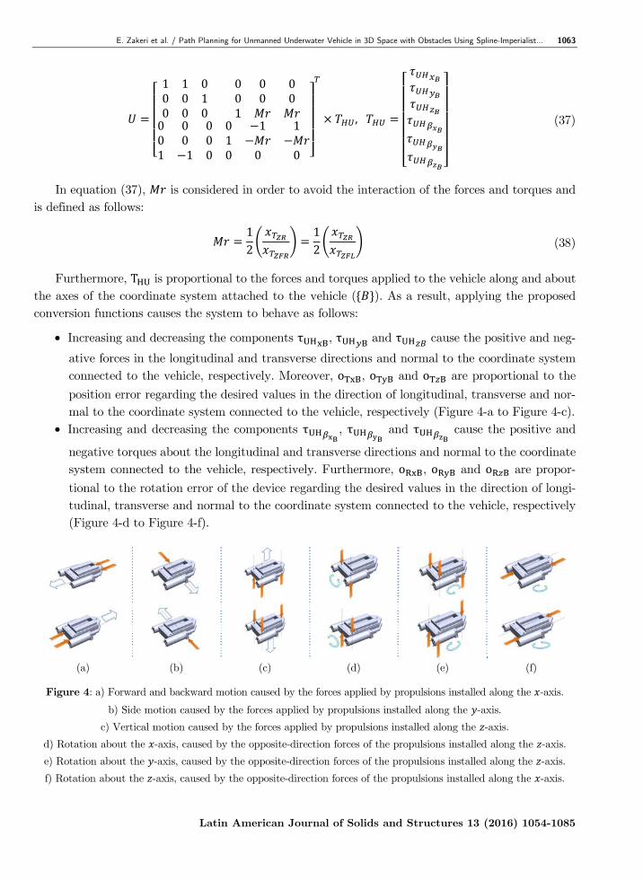
Furthermore, T is proportional to the forces and torques applied to the vehicle along and about the axes of the coordinate system attached to the vehicle ( ). As a result, applying the proposed conversion functions causes the system to behave as follows:

Increasing and decreasing the components τ , τ and τ cause the positive and neg-

ative forces in the longitudinal and transverse directions and normal to the coordinate system connected to the vehicle, respectively. Moreover, o , o and o are proportional to the

position error regarding the desired values in the direction of longitudinal, transverse and nor-mal to the coordinate system connected to the vehicle, respectively (Figure 4-a to Figure 4-c).

Increasing and decreasing the components τ , τ and τ cause the positive and

negative torques about the longitudinal and transverse directions and normal to the coordinate system connected to the vehicle, respectively. Furthermore, o , o and o are propor-

tional to the rotation error of the device regarding the desired values in the direction of longi-tudinal, transverse and normal to the coordinate system connected to the vehicle, respectively (Figure 4-d to Figure 4-f).

(a) (b) (c) (d) (e) (f)

Figure 4: a) Forward and backward motion caused by the forces applied by propulsions installed along the -axis.

b) Side motion caused by the forces applied by propulsions installed along the -axis.

c) Vertical motion caused by the forces applied by propulsions installed along the -axis.

d) Rotation about the -axis, caused by the opposite-direction forces of the propulsions installed along the -axis.

e) Rotation about the -axis, caused by the opposite-direction forces of the propulsions installed along the -axis.

f) Rotation about the -axis, caused by the opposite-direction forces of the propulsions installed along the -axis.



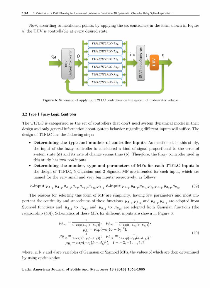
Now, according to mentioned points, by applying the six controllers in the form shown in Figure 5, the UUV is controllable at every desired state.

Figure 5: Schematic of applying IT2FLC controllers on the system of underwater vehicle.

3.2 Type-1 Fuzzy Logic Controller

The T1FLC is categorized as the set of controllers that don’t need system dynamical model in their design and only general information about system behavior regarding different inputs will suffice. The design of T1FLC has the following steps:

Determining the type and number of controller inputs: As mentioned, in this study, the input of the fuzzy controller is considered a kind of signal proportional to the error of system state ( ) and its rate of change versus time ( ). Therefore, the fuzzy controller used in this study has two real inputs.

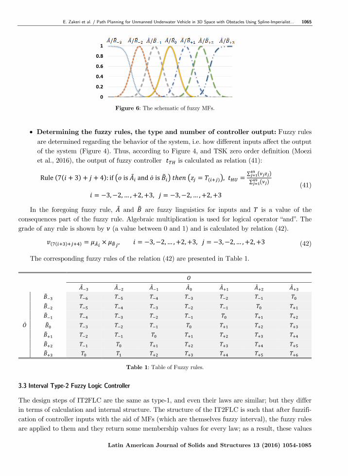
Determining the number, type and parameters of MFs for each T1FLC input: In the design of T1FLC, 5 Gaussian and 2 Sigmoid MF are intended for each input, which are named for the very small and very big inputs, respectively, as follows:

-input: , , , , , , , -input: , , , , , , (39)

The reasons for selecting this form of MF are simplicity, having few parameters and most im-portant the continuity and smoothness of these functions. , and , are adopted from

Sigmoid functions and to and to are adopted from Gaussian functions (the

relationship (40)). Schematics of these MFs for different inputs are shown in Figure 6.

, ,

,

, ,

, 2, 1, … , 1, 2

(40)

where, a, b, c and d are variables of Gaussian or Sigmoid MFs, the values of which are then determined by using optimization.



Figure 6: The schematic of fuzzy MFs.

Determining the fuzzy rules, the type and number of controller output: Fuzzy rules

are determined regarding the behavior of the system, i.e. how different inputs affect the output of the system (Figure 4). Thus, according to Figure 4, and TSK zero order definition (Moezi et al., 2016), the output of fuzzy controller is calculated as relation (41):

Rule 7 3 4 : if is and is ,∑

∑

3, 2, … , 2, 3, 3, 2, … , 2, 3

(41)

In the foregoing fuzzy rule, and are fuzzy linguistics for inputs and is a value of the consequences part of the fuzzy rule. Algebraic multiplication is used for logical operator “and”. The grade of any rule is shown by (a value between 0 and 1) and is calculated by relation (42).

, 3, 2, … , 2, 3, 3, 2,… , 2, 3 (42)

The corresponding fuzzy rules of the relation (42) are presented in Table 1.

Table 1: Table of Fuzzy rules.

3.3 Interval Type-2 Fuzzy Logic Controller

The design steps of IT2FLC are the same as type-1, and even their laws are similar; but they differ in terms of calculation and internal structure. The structure of the IT2FLC is such that after fuzzifi-cation of controller inputs with the aid of MFs (which are themselves fuzzy interval), the fuzzy rules are applied to them and they return some membership values for every law; as a result, these values



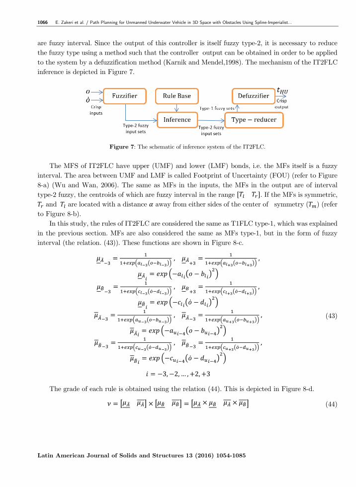
are fuzzy interval. Since the output of this controller is itself fuzzy type-2, it is necessary to reduce the fuzzy type using a method such that the controller output can be obtained in order to be applied to the system by a defuzzification method (Karnik and Mendel,1998). The mechanism of the IT2FLC inference is depicted in Figure 7.

Figure 7: The schematic of inference system of the IT2FLC.

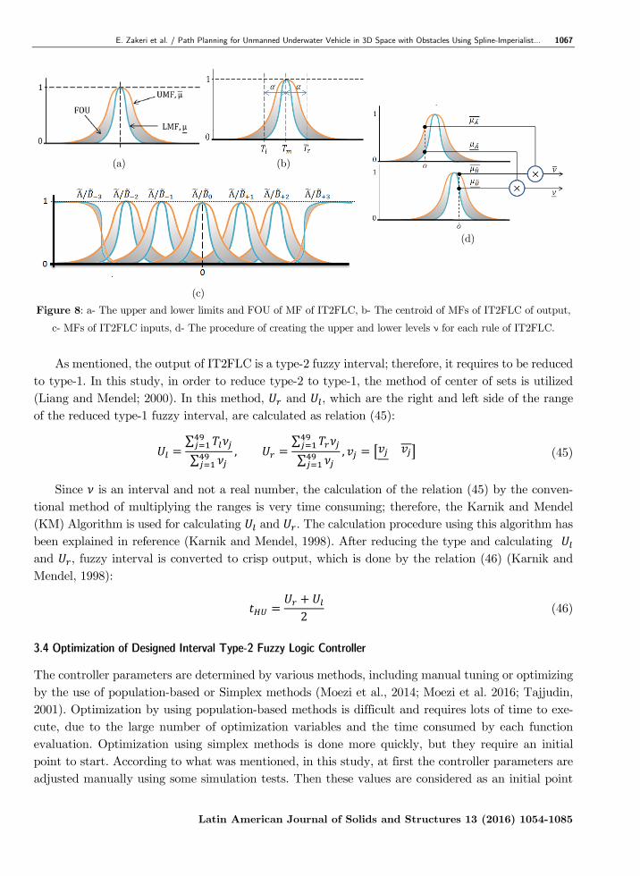
The MFS of IT2FLC have upper (UMF) and lower (LMF) bonds, i.e. the MFs itself is a fuzzy

interval. The area between UMF and LMF is called Footprint of Uncertainty (FOU) (refer to Figure 8-a) (Wu and Wan, 2006). The same as MFs in the inputs, the MFs in the output are of interval type-2 fuzzy, the centroids of which are fuzzy interval in the range . If the MFs is symmetric,

and are located with a distance away from either sides of the center of symmetry ( ) (refer to Figure 8-b).

In this study, the rules of IT2FLC are considered the same as T1FLC type-1, which was explained in the previous section. MFs are also considered the same as MFs type-1, but in the form of fuzzy interval (the relation. (43)). These functions are shown in Figure 8-c.

, ,

, ,

, ,

, ,

3, 2, … , 2, 3

(43)

The grade of each rule is obtained using the relation (44). This is depicted in Figure 8-d.

(44)



(d)

(b) (a)

(c)

Figure 8: a- The upper and lower limits and FOU of MF of IT2FLC, b- The centroid of MFs of IT2FLC of output,

c- MFs of IT2FLC inputs, d- The procedure of creating the upper and lower levels ν for each rule of IT2FLC.

As mentioned, the output of IT2FLC is a type-2 fuzzy interval; therefore, it requires to be reduced

to type-1. In this study, in order to reduce type-2 to type-1, the method of center of sets is utilized (Liang and Mendel; 2000). In this method, and , which are the right and left side of the range of the reduced type-1 fuzzy interval, are calculated as relation (45):

∑

∑,

∑

∑, (45)

Since is an interval and not a real number, the calculation of the relation (45) by the conven-tional method of multiplying the ranges is very time consuming; therefore, the Karnik and Mendel (KM) Algorithm is used for calculating and . The calculation procedure using this algorithm has been explained in reference (Karnik and Mendel, 1998). After reducing the type and calculating and , fuzzy interval is converted to crisp output, which is done by the relation (46) (Karnik and Mendel, 1998):

2 (46)

3.4 Optimization of Designed Interval Type-2 Fuzzy Logic Controller

The controller parameters are determined by various methods, including manual tuning or optimizing by the use of population-based or Simplex methods (Moezi et al., 2014; Moezi et al. 2016; Tajjudin, 2001). Optimization by using population-based methods is difficult and requires lots of time to exe-cute, due to the large number of optimization variables and the time consumed by each function evaluation. Optimization using simplex methods is done more quickly, but they require an initial point to start. According to what was mentioned, in this study, at first the controller parameters are adjusted manually using some simulation tests. Then these values are considered as an initial point



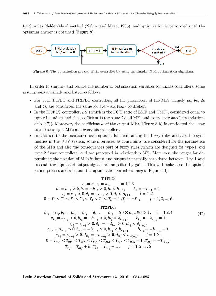
for Simplex Nelder-Mead method (Nelder and Mead, 1965), and optimization is performed until the optimum answer is obtained (Figure 9).

Figure 9: The optimization process of the controller by using the simplex N-M optimization algorithm.

In order to simplify and reduce the number of optimization variables for fuzzes controllers, some

assumptions are made and listed as follows:

For both T1FLC and IT2FLC controllers, all the parameters of the MFs, namely s, s, s and s, are considered the same for every six fuzzy controller.

In the IT2FLC controller, (which is the FOU ratio of LMF and UMF), considered equal to upper boundary and this coefficient is the same for all MFs and every six controllers (relation-ship (47)). Moreover, the coefficient of the output MFs (Figure 8-b) is considered the same in all the output MFs and every six controllers.

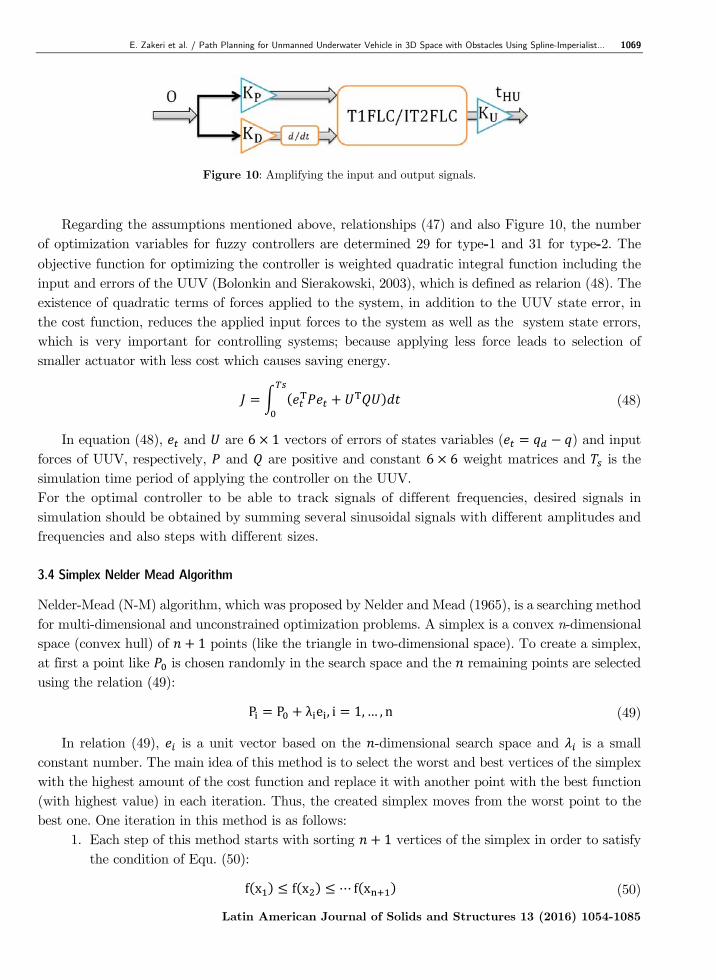
In addition to the mentioned assumptions, for maintaining the fuzzy rules and also the sym-metries in the UUV system, some interfaces, as constraints, are considered for the parameters of the MFs and also the consequences part of fuzzy rules (which are designed for type-1 and type-2 fuzzy controllers) and are presented in relationship (47). Moreover, the ranges for de-termining the position of MFs in input and output is normally considered between -1 to 1 and instead, the input and output signals are amplified by gains. This will make ease the optimi-zation process and selection the optimization variables ranges (Figure 10).

: , , 1,2,3

0, 0, , 1 0, 0, , 1, 2.

0 1, , 1, 2, … , 6

: , , , 1, 1,2,3

0, 0, , 1 0, 0, ,

0, 0, , 1 0, 0, , 1, 2.

0 1 , , , , 1, 2, … , 6

(47)



Figure 10: Amplifying the input and output signals.

Regarding the assumptions mentioned above, relationships (47) and also Figure 10, the number

of optimization variables for fuzzy controllers are determined 29 for type-1 and 31 for type-2. The objective function for optimizing the controller is weighted quadratic integral function including the input and errors of the UUV (Bolonkin and Sierakowski, 2003), which is defined as relarion (48). The existence of quadratic terms of forces applied to the system, in addition to the UUV state error, in the cost function, reduces the applied input forces to the system as well as the system state errors, which is very important for controlling systems; because applying less force leads to selection of smaller actuator with less cost which causes saving energy.

(48)

In equation (48), and are 6 1 vectors of errors of states variables ( ) and input forces of UUV, respectively, and are positive and constant 6 6 weight matrices and is the simulation time period of applying the controller on the UUV. For the optimal controller to be able to track signals of different frequencies, desired signals in simulation should be obtained by summing several sinusoidal signals with different amplitudes and frequencies and also steps with different sizes. 3.4 Simplex Nelder Mead Algorithm

Nelder-Mead (N-M) algorithm, which was proposed by Nelder and Mead (1965), is a searching method for multi-dimensional and unconstrained optimization problems. A simplex is a convex n-dimensional space (convex hull) of 1 points (like the triangle in two-dimensional space). To create a simplex, at first a point like is chosen randomly in the search space and the remaining points are selected using the relation (49):

P P λ e , i 1, … , n (49)

In relation (49), is a unit vector based on the -dimensional search space and is a small constant number. The main idea of this method is to select the worst and best vertices of the simplex with the highest amount of the cost function and replace it with another point with the best function (with highest value) in each iteration. Thus, the created simplex moves from the worst point to the best one. One iteration in this method is as follows:

1. Each step of this method starts with sorting 1 vertices of the simplex in order to satisfy the condition of Equ. (50):

f x f x ⋯ f x (50)



In Equ. (50) , and are the best and the worst points, respectively. 2. Calculating the center of gravity of points of the best points by using Equ. (51) or calcu-

lating the center of gravity of all points except the point and reflecting the worst point regarding the center of gravity which is given in Equ. (52).

x1n

x (51)

x x x x 2x x (52)

f f x (53)

3. Regarding the relative value of , obtained from the Equ. (53), one of the following 4 modes may occur:

a f f b f f f c f f f d f f (54)

If the condition “a” is satisfied, the expansion point is calculated using the relationship (55) in the same direction.

x x x x 3x 2x (55)

Finally, after calculating the expansion point, its value is obtained as . However, if , is replaced with ; otherwise, is replaced with .

If the condition “b” is satisfied, is replaced with . If the condition “c” is satisfied, the outside contraction is performed and is calculated using the

relation (56):

x x12x x

32x

12x , f f x (56)

However, if , is replaced with and iteration ends; otherwise, it goes to step 4 and shrinking takes place.

If the condition “d” is satisfied, the inside contraction is performed and is calculated using the relation (57):

x x12x x

12x

12x (57)

However, if , is replaced with ; otherwise, it goes to step 4 and shrinking takes place.

Shrinking: The dividing action means that the search operation around is useless and simplex should be crushed (Shrink) and go to near . Now, the new points are calculated as relation (58):

V x12x x , i 2, … , n 1 (58)



Then is calculated at all new points. Simplex unsorted vertices are , , … , at the next iteration. 4 GENERATING THE OPTIMAL PATH WITHOUT COLLISION USING SPLINE-ICA

In this section, a short path without collision is intended as the aim of generating the optimal path. Moreover, smoothness of the created path is another feature observed in this method. Therefore, to generate the path from the starting point P to the target point P in three-dimensional space, at first

some points in the desired space and in the specified range is selected, which are known as control points. Furthermore, the starting and target points are considered as the first and last points of the path in the points set. Then, by using spline method, a curve is passed on these points (De Boor, 1978). Determining the location of these points by the aid of ICA leads to a smooth and short path without colliding obstacles. Any point in the surrounding environment of the UUV that is owned to the obstacle, takes a numerical value. This value is used in the optimization in order to avoid collisions with obstacles (it is added to the objective function as penalty). Therefore, the objective function is defined in such a way that the resulting path has the shortest length and avoids colliding the obstacles. 4.1 Generating the Path by Using Spline

As mentioned, the locations of the control points are selected in such a way that a short path without collision is achieved. As a result, for selecting these points evolutionary optimization methods are used, which are suitable options. If n control points are considered to generate a path by spline method, the desired path is generated as relation (59) to (61) (Zakeri and Farahat, 2015; Moezi et al., 2015):

, , , , , , , , (59)

SPL , . . . ,

SPL , . . . ,

SPL , . . . ,

1…

1

(60)

∈ 0 1 (61)

In relation (59), s are control points of spline curve (De Boor, 1978), f , f , f s are path points

that change from the starting point to the target point by changing k from k to k , i.e. they create

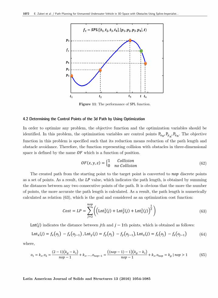
the path. SPL is a function that passes a spline curve through the input points, and returns the desired point (Moezi et al., 2015). The performance of this function is shown in Figure 11.



Figure 11: The performance of SPL function.

4.2 Determining the Control Points of the 3d Path by Using Optimization

In order to optimize any problem, the objective function and the optimization variables should be identified. In this problem, the optimization variables are control points P , P , P . The objective

function in this problem is specified such that its reduction means reduction of the path length and obstacle avoidance. Therefore, the function representing collision with obstacles in three-dimensional space is defined by the name which is a function of position.

, , 10

(62)

The created path from the starting point to the target point is converted to discrete points as a set of points. As a result, the value, which indicates the path length, is obtained by summing the distances between any two consecutive points of the path. It is obvious that the more the number of points, the more accurate the path length is calculated. As a result, the path length is numerically calculated as relation (63), which is the goal and considered as an optimization cost function:

Lnt Lnt Lnt (63)

Lnt indicates the distance between th and 1th points, which is obtained as follows:

Lnt , Lnt , Lnt (64)

where,

,2 1

1, … ,

1 11

, | 1 (65)



As previously mentioned, represents the collision value and if collision happens, the cost function is provided with penalty. Therefore, the penalty function of collision is considered as relation (66).

0 ∑ 0

10 ∑, 1, 2, … , 5

, , , 1, 2, … , (66)

Therefore, the cost function with the function of collision penalty is considered as relation (67):

(67)

By reducing the cost amount of relation (67), a short path without colliding with obstacles in the environment is achieved. 4.3 Creating Desired Signals from Optimal Generated Path

After the optimal path and the corresponding parameters are obtained, desired signals should be produced to control the vehicle. For this purpose, it is assumed that the UUV travels the path with a constant velocity V , and also the X-Y plane of {B} is parallel to the water level and the longitudinal direction of vehicle is tangent to the path projected on the , plane of the . Therefore, considering a constant velocity on the path, the relation (68) is obtained (Zakeri and Farahat, 2015; Moezi et al., 2015).

0 (68)

Also, According to mentioned condition, the desired signals for the UUV are obtained as below:

, , , 2 ,

0(69)

Where According to relation (86), is achieved as follows:

(70)

4.4 Imperialist Competitive Algorithm

Imperialist Competitive Algorithm (ICA) is originally inspired by the procedure of imprialist coutries in obtaining power and as a result the optimization method is relatively strong (Atashpaz and Lucas, 2007). In this algorithm, all countries are divided into two categories of imprialist and colony coun-tries. The imprialistic competition is the main part of this algorithm which leads to the convergence



of the objective function toward the optimal point. In ICA, each of the population vectors is originally called a country and is considered as follows:

country p p p … p (71)

where, is the number of variables or the number of dimension of the optimization problem. At the beginning of optimization process, countries are scattered randomly in optimization space and of the most powerful countries are considered as the empires. In order to divide and assign colonial countries to empires, the colonists cost values (cost and inverse of power are proportional with each other) should be normalized as relation (72):

(72)

where, is the th colonial cost and is its normalized value. As a result, the normalized power of th colonial is as relation (73):

∑ (73)

From another point of view, the normalized power of each colonial specifies its contribution in colonizing the colony countries. As a result, the initial colonies of th empire is as relation (74).

. . . (74)

In the above equation, . . is the initial number of colonies of each empire and is the total colonial countries. As a result, this number of colonies are randomly selected for each empire. Then colonial countries move toward their colonizing countries. Any country moves toward its colonizing country by the distance and the angle , which are random values (Equ. (75)).

~ 0, , ~ , (75)

where, is a value greater than one, is the distance between the colonial country to its colonizing country, is a positive and arbitrary variable and is usually considered as . After moving to the

toward the colonizing country, if the power of colonial country becomes more than the colonizing country, they are changed. The total cost of the th empire is calculated as follows:

. . (76)

Where, is a positive value smaller than one. This algorithm is such that at each step the weakest colonial country of the weakest colonizing empire is separated from it and joins to one of the rest of the empires regarding a probability proportional to that empire power. In order to start the compe-tition between empires, at first the probability of each of them to accept a new colony is calculated. The normalized value of the total cost of the th empire (N. T. C. ) is calculated as relation (79). As a result, the probability of ownership of any empire is calculated as relation (78):

. . . . . . . (77)



. . .

∑ . . . (78)

where, P is the probability of ownership of the th empire. To select the host empire, the vector

is built from the ownership probability of the empires as relation (79):

… (79)

Then another vector , the length of which is the same as vector , is built. The components of this vector are random values between zero and one, with a uniform probability distribution (relation (80)).

… , , , , … , ~ 0,1 (80)

Then, the vector is obtained by subtracting vector from vector , as relation (81):

(81)

The component number of vector that has the maximum value is the number of host empire. In the end, all of the empires, except the strongest one, fail and all the countries are dominated by the most powerful empire in one place with equal power. In principle, all converge to a point which is considered to be the end of the optimization process. 5 SIMULATION AND RESULTS

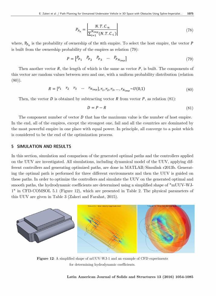
In this section, simulation and comparison of the generated optimal paths and the controllers applied on the UUV are investigated. All simulations, including dynamical model of the UUV, applying dif-ferent controllers and generating optimized paths, are done in MATLAB/Simulink r2013b. Generat-ing the optimal path is performed for three different environments and then the UUV is guided on these paths. In order to optimize the controllers and simulate the UUV on the generated optimal and smooth paths, the hydrodynamic coefficients are determined using a simplified shape of "mUUV-WJ-1" in CFD-COMSOL 5.1 (Figure 12), which are presented in Table 2. The physical parameters of this UUV are given in Table 3 (Zakeri and Farahat, 2015).

Figure 12: A simplified shape of mUUV-WJ-1 and an example of CFD experiments

for determining hydrodynamic coefficients.



Added mass coefficient Damping and friction coefficients 1.49 | | 5.67 0.0117

1.23 | | 3.62 0.0102

1.98 | | 7.35 0.00981

0.011 . | | 0.0155 0.000191

0.0165 . | | 0.0183 0.000211

0.0086 . | | 0.0126 0.000311

Table 2: Hydrodynamic coefficients obtained via CFD simulations for “mUUV-WJ-1”

Parameters Values

2.36

Diag 0.0121 0.0160 0.0253 .

2.33

1000

0 0 0

y , y , x, x , x , y , x , y 0.055, 0.055,0, 0.11,0.11,0.065,0.11, 0.065

9.806

Table 3: The values of physical parameters of “mUUV-WJ-1” in simulation.

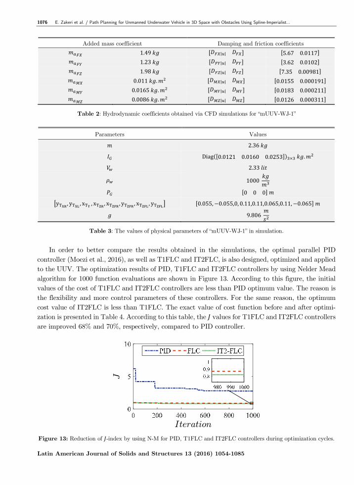
In order to better compare the results obtained in the simulations, the optimal parallel PID controller (Moezi et al., 2016), as well as T1FLC and IT2FLC, is also designed, optimized and applied to the UUV. The optimization results of PID, T1FLC and IT2FLC controllers by using Nelder Mead algorithm for 1000 function evaluations are shown in Figure 13. According to this figure, the initial values of the cost of T1FLC and IT2FLC controllers are less than PID optimum value. The reason is the flexibility and more control parameters of these controllers. For the same reason, the optimum cost value of IT2FLC is less than T1FLC. The exact value of cost function before and after optimi-zation is presented in Table 4. According to this table, the values for T1FLC and IT2FLC controllers are improved 68% and 70%, respectively, compared to PID controller.

Figure 13: Reduction of -index by using N-M for PID, T1FLC and IT2FLC controllers during optimization cycles.



IT2FLC T1FLC PID Controller Type

Optimal Initial Optimal Initial Optimal Initial Condition

0.8208 0.9694 0.8685 0.9712 2.7495 6.1819 Value of J index

Table 4: The initial and optimum amount of -index for each three controllers.

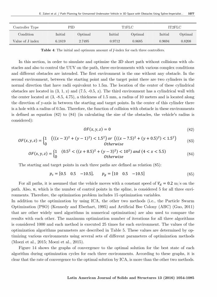
In this section, in order to simulate and optimize the 3D short path without collisions with ob-stacles and also to control the UUV on the path, three environments with various complex conditions and different obstacles are intended. The first environment is the one without any obstacle. In the second environment, between the starting point and the target point there are two cylinders in the normal direction that have radii equivalent to 1.5m. The location of the center of these cylindrical obstacles are located in (3, 1, z) and (7.5, -0.5, z). The third environment has a cylindrical wall with the center located at (3, -8.5, 4.75), a thickness of 1.5 mm, a radius of 10 meters and is located along the direction of y-axis in between the starting and target points. In the center of this cylinder there is a hole with a radius of 0.5m. Therefore, the function of collision with obstacle in these environments is defined as equation (82) to (84) (in calculating the size of the obstacles, the vehicle's radius is considered):

, , 0 (82)

, , 1 3 1 1.5 7.5 0.5 1.50

(83)

, , 1 0.5 8.5 3 10 4 5.50

(84)

The starting and target points in each three paths are defined as relation (85):

0.5 0.5 10.5 , 10 0.5 10.5 (85)

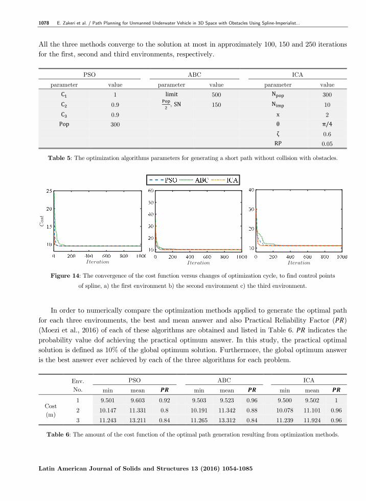
For all paths, it is assumed that the vehicle moves with a constant speed of 0.2 m/s on the path. Also, , which is the number of control points in the spline, is considered 5 for all three envi-ronments. Therefore, the optimization problem includes 15 optimization variables. In addition to the optimization by using ICA, the other two methods (i.e., the Particle Swarm Optimization (PSO) (Kennedy and Eberhart, 1995) and Artificial Bee Colony (ABC) (Guo, 2011) that are other widely used algorithms in numerical optimization) are also used to compare the results with each other. The maximum optimization number of iterations for all three algorithms is considered 1000 and each method is executed 25 times for each environment. The values of the optimization algorithms parameters are described in Table 5. These values are determined by op-timizing various environments using several sets of different parameters of optimization methods (Moezi et al., 2015; Moezi et al., 2015).

Figure 14 shows the graphs of convergence to the optimal solution for the best state of each algorithm during optimization cycles for each three environments. According to these graphs, it is clear that the rate of convergence to the optimal solution by ICA, is more than the other two methods.



All the three methods converge to the solution at most in approximately 100, 150 and 250 iterations for the first, second and third environments, respectively.

ICA ABC PSO

value parameter value parameter value parameter

300 N 500 limit 1 C

10 N 150 , SN 0.9 C

2 x 0.9 C

π/4 θ 300 Pop

0.6 ζ

0.05 RP

Table 5: The optimization algorithms parameters for generating a short path without collision with obstacles.

Figure 14: The convergence of the cost function versus changes of optimization cycle, to find control points

of spline, a) the first environment b) the second environment c) the third environment.

In order to numerically compare the optimization methods applied to generate the optimal path

for each three environments, the best and mean answer and also Practical Reliability Factor ( ) (Moezi et al., 2016) of each of these algorithms are obtained and listed in Table 6. indicates the probability value dof achieving the practical optimum answer. In this study, the practical optimal solution is defined as 10% of the global optimum solution. Furthermore, the global optimum answer is the best answer ever achieved by each of the three algorithms for each problem.

ICA ABC PSO Env. No.

mean min mean min mean min

1 9.502 9.500 0.96 9.523 9.503 0.92 9.603 9.501 1 Cost (m)

0.96 11.101 10.078 0.88 11.342 10.191 0.8 11.331 10.147 2

0.96 11.924 11.239 0.84 13.312 11.265 0.84 13.211 11.243 3

Table 6: The amount of the cost function of the optimal path generation resulting from optimization methods.



According to Table 6, it is clear that the minimum value of the cost for ICA for each three environments is less than PSO and ABC. This is also true for the average cost; such that the average cost of ICA is less than PSO and ABC by 1% and 0.2%, respectively, in the first environment, 2.1% and 2.9%, respectively, in the second environment and 10.8% and 11.6%, respectively, in the third environment. This comparison shows that in more complex environments ICA has a better optimiza-tion value than the other two algorithms. Furthermore, the larger size of for ICA, comparing with PSO and ABC in all three environments, shows that ICA achieves the optimum solution with more reliability. Since the cost of ICA in all three environments is less than PSO and ABC, the values obtained by this algorithm are used for generating optimal paths in all three environments.

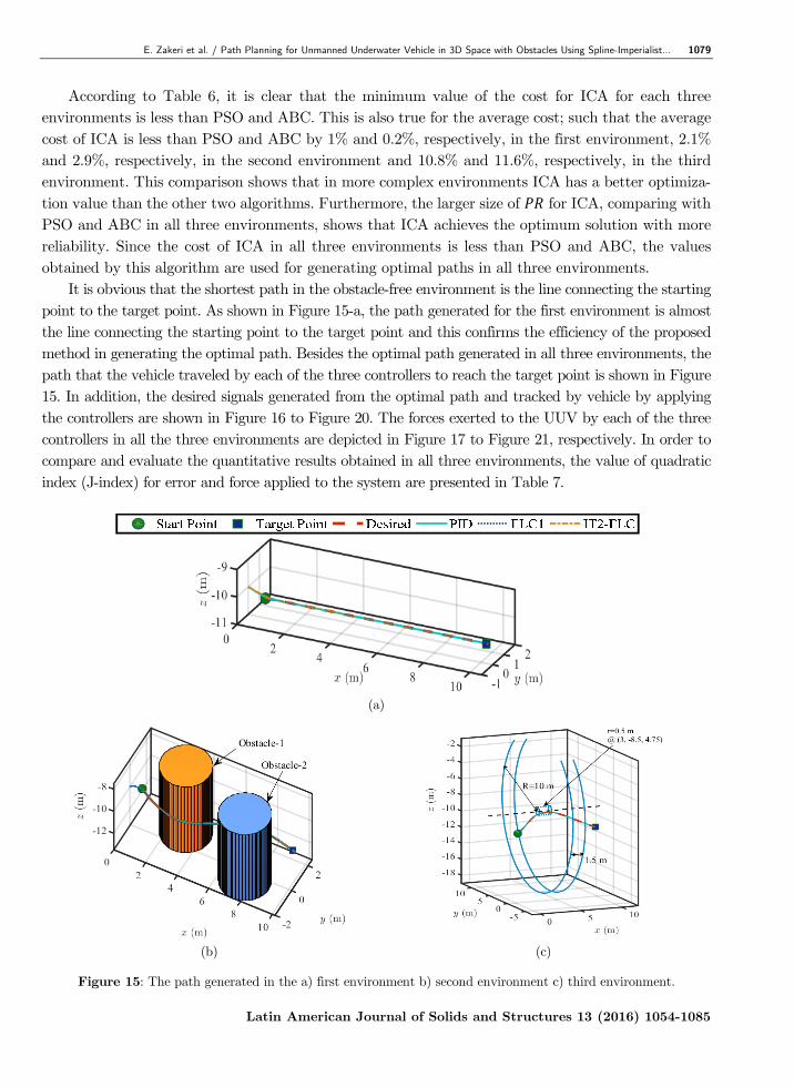
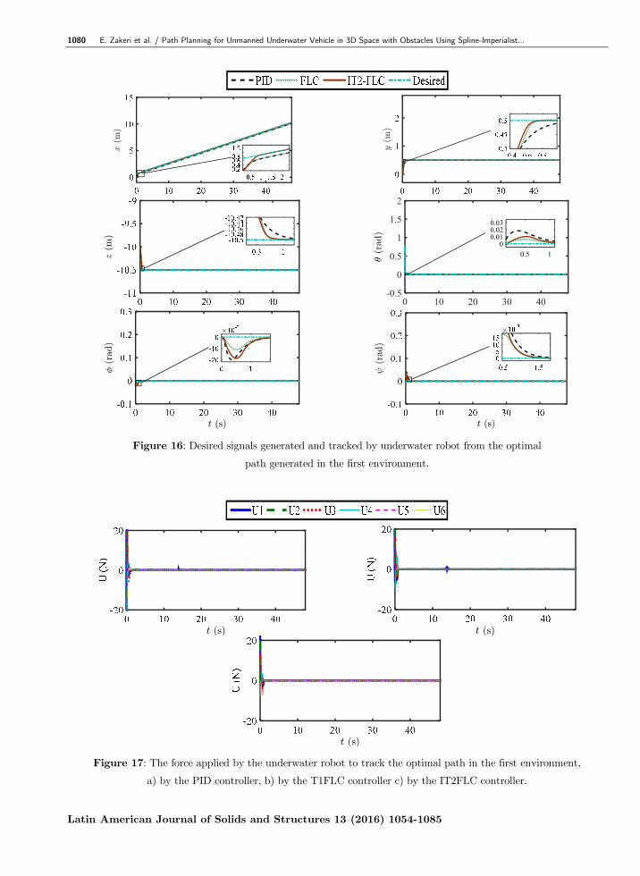
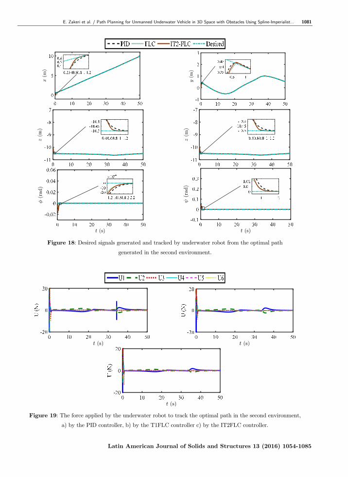
It is obvious that the shortest path in the obstacle-free environment is the line connecting the starting point to the target point. As shown in Figure 15-a, the path generated for the first environment is almost the line connecting the starting point to the target point and this confirms the efficiency of the proposed method in generating the optimal path. Besides the optimal path generated in all three environments, the path that the vehicle traveled by each of the three controllers to reach the target point is shown in Figure 15. In addition, the desired signals generated from the optimal path and tracked by vehicle by applying the controllers are shown in Figure 16 to Figure 20. The forces exerted to the UUV by each of the three controllers in all the three environments are depicted in Figure 17 to Figure 21, respectively. In order to compare and evaluate the quantitative results obtained in all three environments, the value of quadratic index (J-index) for error and force applied to the system are presented in Table 7.

(a)

(b) (c)

Figure 15: The path generated in the a) first environment b) second environment c) third environment.



Figure 16: Desired signals generated and tracked by underwater robot from the optimal

path generated in the first environment.

Figure 17: The force applied by the underwater robot to track the optimal path in the first environment,

a) by the PID controller, b) by the T1FLC controller c) by the IT2FLC controller.

0 10 20 30 40-0.5

0

0.5

1

1.5

2

0.5 10

0.010.020.03



Figure 18: Desired signals generated and tracked by underwater robot from the optimal path

generated in the second environment.

Figure 19: The force applied by the underwater robot to track the optimal path in the second environment,

a) by the PID controller, b) by the T1FLC controller c) by the IT2FLC controller.



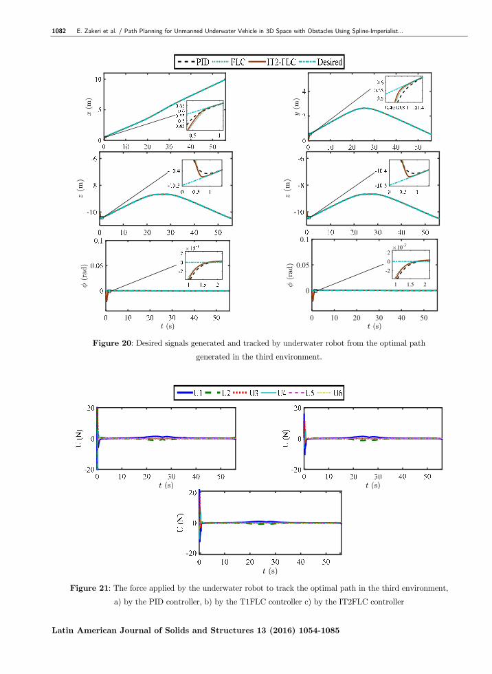
Figure 20: Desired signals generated and tracked by underwater robot from the optimal path

generated in the third environment.

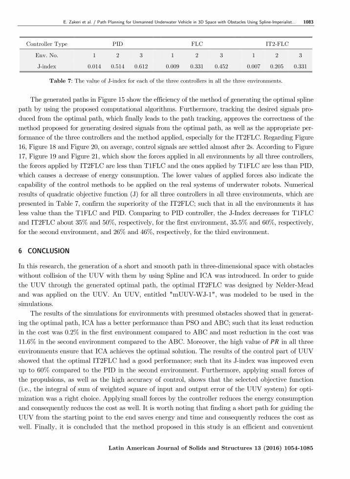
Figure 21: The force applied by the underwater robot to track the optimal path in the third environment,

a) by the PID controller, b) by the T1FLC controller c) by the IT2FLC controller

0 10 20 30 40 50

0

0.05

0.1

1 1.5 2

10-3

-202



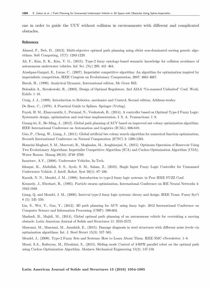
IT2-FLC FLC PID Controller Type

3 2 1 3 2 1 3 2 1 Env. No.

0.331 0.205 0.007 0.452 0.331 0.009 0.612 0.514 0.014 J-index

Table 7: The value of J-index for each of the three controllers in all the three environments.

The generated paths in Figure 15 show the efficiency of the method of generating the optimal spline

path by using the proposed computational algorithms. Furthermore, tracking the desired signals pro-duced from the optimal path, which finally leads to the path tracking, approves the correctness of the method proposed for generating desired signals from the optimal path, as well as the appropriate per-formance of the three controllers and the method applied, especially for the IT2FLC. Regarding Figure 16, Figure 18 and Figure 20, on average, control signals are settled almost after 2s. According to Figure 17, Figure 19 and Figure 21, which show the forces applied in all environments by all three controllers, the forces applied by IT2FLC are less than T1FLC and the ones applied by T1FLC are less than PID, which causes a decrease of energy consumption. The lower values of applied forces also indicate the capability of the control methods to be applied on the real systems of underwater robots. Numerical results of quadratic objective function (J) for all three controllers in all three environments, which are presented in Table 7, confirm the superiority of the IT2FLC; such that in all the environments it has less value than the T1FLC and PID. Comparing to PID controller, the J-Index decreases for T1FLC and IT2FLC about 35% and 50%, respectively, for the first environment, 35.5% and 60%, respectively, for the second environment, and 26% and 46%, respectively, for the third environment. 6 CONCLUSION

In this research, the generation of a short and smooth path in three-dimensional space with obstacles without collision of the UUV with them by using Spline and ICA was introduced. In order to guide the UUV through the generated optimal path, the optimal IT2FLC was designed by Nelder-Mead and was applied on the UUV. An UUV, entitled "mUUV-WJ-1", was modeled to be used in the simulations.

The results of the simulations for environments with presumed obstacles showed that in generat-ing the optimal path, ICA has a better performance than PSO and ABC; such that its least reduction in the cost was 0.2% in the first environment compared to ABC and most reduction in the cost was 11.6% in the second environment compared to the ABC. Moreover, the high value of in all three environments ensure that ICA achieves the optimal solution. The results of the control part of UUV showed that the optimal IT2FLC had a good performance; such that its J-index was improved even up to 60% compared to the PID in the second environment. Furthermore, applying small forces of the propulsions, as well as the high accuracy of control, shows that the selected objective function (i.e., the integral of sum of weighted square of input and output error of the UUV system) for opti-mization was a right choice. Applying small forces by the controller reduces the energy consumption and consequently reduces the cost as well. It is worth noting that finding a short path for guiding the UUV from the starting point to the end saves energy and time and consequently reduces the cost as well. Finally, it is concluded that the method proposed in this study is an efficient and convenient



one in order to guide the UUV without collision in environments with different and complicated obstacles. References

Ahmed, F., Deb, D., (2013). Multi-objective optimal path planning using elitist non-dominated sorting genetic algo-rithms. Soft Computing, 17(7): 1283-1229.

Ali, F., Kim, E. K., Kim, Y. G., (2015). Type-2 fuzzy ontology-based semantic knowledge for collision avoidance of autonomous underwater vehicles. Inf. Sci. (Ny) 295: 441–464.

Atashpaz-Gargari, E., Lucas, C., (2007). Imperialist competitive algorithm: An algorithm for optimization inspired by imperialistic competition, IEEE Congress on Evolutionary Computation, 2007: 4661-4667.

Baruh, H., (1999). Analytical Dynamic, International edition, Mc Graw Hill.

Bolonkin A., Sierakowski, R., (2003). Design of Optimal Regulators. 2nd AIAA “Un-manned Unlimited” Conf. Work. Exhib: 1–18.

Craig, J. J., (1989). Introduction to Robotics, mechanics and Control, Second edition, Addison-wesley.

De Boor, C., (1978). A Practical Guide to Splines. Springer (Verlag).

Fayek, H. M., Elamvazuthi, I., Perumal, N., Venkatesh, B., (2014). A controller based on Optimal Type-2 Fuzzy Logic: Systematic design, optimization and real-time implementation. I. S. A. Transactions: 1–9.

Guang-lei, Z., He-Ming, J., (2012). Global path planning of AUV based on improved ant colony optimization algorithm. IEEE International Conference on Automation and Logistics (ICAL): 606-610.

Guo, P., Cheng, W., Liang, J., (2011). Global artificial bee colony search algorithm for numerical function optimization, Seventh International Conference on Natural Computation (ICNC) 3: 1280-1283.

Hosseini-Moghari, S. M., Morovati, R., Moghadas, M., Araghinejad, S., (2015). Optimum Operation of Reservoir Using Two Evolutionary Algorithms: Imperialist Competitive Algorithm (ICA) and Cuckoo Optimization Algorithm (COA). Water Resour. Manag 29(10): 3749–3769.

Inzartsev, A.V., (2008). Underwater Vehicles, In-Tech.

Ishaque, K., Abdullah, S. S., Ayob, S. M., Salam, Z., (2010). Single Input Fuzzy Logic Controller for Unmanned Underwater Vehicle. J. Intell. Robot. Syst 59(1): 87–100.

Karnik, N. N., Mendel, J. M., (1998). Introduction to type-2 fuzzy logic systems. in Proc IEEE FUZZ Conf.

Kennedy, J., Eberhart, R., (1995). Particle swarm optimization, International Conference on IEE Neural Networks 4: 1942-1948.

Liang, Q. and Mendel, J. M., (2000). Interval type-2 fuzzy logic systems: theory and design. IEEE Trans. Fuzzy Sys”t 8 (5): 535–550.

Liu, S., Wei, Y., Gao, Y., (2012). 3D path planning for AUV using fuzzy logic. 2012 International Conference on Computer Science and Information Processing (CSIP): 599-603.

Mashadi, B., Majidi, M., (2014), Global optimal path planning of an autonomous vehicle for overtaking a moving obstacle. Latin American Journal of Solids and Structures 11: 2555-2572.

Masoumi, M., Masoumi, M., Jamshidi, E., (2015). Damage diagnosis in steel structures with different noise levels via optimization algorithms. Int. J. Steel Struct 15(3): 557–565.

Mendel, J., (2009). Type-2 Fuzzy Sets and Systems: How to Learn About Them. IEEE SMC eNewsletter: 1–8.

Moezi, S.A., Rafeeyan, M., Ebrahimi, S., (2015). Sliding mode Control of 3-RPR parallel robot on the optimal path using Cuckoo Optimization Algorithm. Modares Mechanical Engineering 15(2): 147-158.



Moezi, S.A., Rafeeyan, M., Zakeri, E., Zare, A., (2016). Simulation and experimental control of a 3-RPR parallel robot using optimal fuzzy controller and fast on/off solenoid valves based on the PWM wave. ISA Transactions 61 (2016): 265-286.

Moezi, S.A., Zakeri, E., Bazargan – Lari, Y., Khalghollah, M., (2014). Fuzzy Logic Control of a Ball on Sphere System. Advances in Fuzzy Systems 2014: 1-6.

Moezi, S.A., Zakeri, E., Bazargan – Lari, Y., Zare, A., (2015). 2&3-Dimensional Optimization of Connecting Rod with Genetic and Modified Cuckoo Optimization Algorithms. IJST, Transactions of Mechanical Engineering 39(M1): 39-49.

Moezi, S.A., Zakeri, E., Bazargan-Lari, Y., Tavallaeinejad, M., (2014). Control of a Ball on Sphere System with Adaptive Neural Network Method for Regulation Purpose. J. Applied Sci., 1 (6).

Moezi, S.A., Zakeri, E., Zare, A., Nedaei, M., (2015). On the application of modified cuckoo optimization algorithm to the crack detection problem of cantilever Euler–Bernoulli beam. Computers & Structures 157: 42-50.

Nag, A., Patel, S.S., Akbar, S.A., (2013). Fuzzy logic based depth control of an autonomous underwater vehicle. In-ternational Multi-Conference on Automation, Computing, Communication, Control and Compressed Sensing (iMac4s): 117-123.

Nelder, J.A., Mead, R., (1965). A simplex for function minimization. Comput J 7:308–13.

Poppinga, J., Birk, A., Pathak, K., Vaskevicius, N., (2011). Fast 6-DOF path planning for Autonomous Underwater Vehicles (AUV) based on 3D plane mapping. IEEE International Symposium on Safety, Security, and Rescue Robotics (SSRR): 345-350.

Tajjudin, M., Ishak, N., Ismail, H., Hezri, M., Rahiman, F., Adnan, R., (2011). Optimized PID Control using Nelder-Mead Method for Electro-hydraulic Actuator Systems. Proc. in IEEE Control Syst. Grad. Res. Colloquium 1: 90–93.

Wu, D., Wan, W., (2006). A simplified type-2 fuzzy logic controller for real-time control. I. S. A. Transactions 45(4): 503–516.

Xu, J., Wang, M., Qiao, L., (2015). Dynamical sliding mode control for the trajectory tracking of underactuated unmanned underwater vehicles. Ocean Eng 105: 54–63.

Zakeri, E., Bazargan-Lari, Y., Eghtesad, M., (2012). Simultaneous Control of GMAW Process and SCARA Robot in Tracking a Circular Path via a Cascade Approach. Trends in Applied Sciences Research 7(10): 845-858.

Zakeri, E., Farahat, S., (2015). Safe path planning and control of an Unmanned Underwater Vehicle (UUV) using particle swarm optimization and fuzzy logic control method. Modares Mechanical Engineering 14(14): 199-210.

Zakeri, E., Farahat, S., (2015). Simulation and Controller Designing of an Unmanned Underwater Vehicle. Master thesis (in Persian), University of Sistan and Bluchestan.

Zakeri, E., Moezi, S.A., Bazargan-Lari, Y., (2013). Control of a Ball on Sphere System with Adaptive Feedback Line-arization method for regulation purpose. Majlesi Journal of Mechatronic Engineering, 2(3): 23-27.

Zakeri, E., Moezi, S.A., Zare, M., Parnian Rad, M., (2014). Control of Puma-560 robot Using Feedback Linearization control method and kalman filter estimator for Regulation and Tracking Purpose. Journal of mathematics and com-puter science 11(2014): 264-276.

Zare, M., Sadeghi, J., Farahat, S., Zakeri, E., (2014). Regulating and Helix Path Tracking for Unmanned Aerial Vehicle (UAV) Using Fuzzy Logic Controllers. Journal of mathematics and computer science 13(2014): 71-89.

Zhang, X., Han, Y., Bai, T., Wei, Y., Ma, K., (2015). H∞ controller design using LMIs for high-speed underwater vehicles in presence of uncertainties and disturbances. Ocean Eng 104: 359–369.

Zhu, D., Yang, Y., Yan, M., (2011). Path planning algorithm for AUV based on a Fuzzy-PSO in dynamic environ-ments. Eighth International Conference on Fuzzy Systems and Knowledge Discovery (FSKD) 1: 525-530.

Zimmermann, H.-J., (1996). fuzzy set theory and its application, third edition. Kluwer Academic Publishers (Boston).

path planning for unmanned underwater vehicle in … · the optimal path is converted to desirable...

Documents