Passive seismic interferometry in the real world:

Application with microseismic and traffic noise

By

Yang Zhao

A dissertation submitted in partial satisfaction of the

requirements for the degree of

Doctor of Philosophy

in

Engineering - Civil and Environmental Engineering

in the

Graduate Division

of the

University of California, Berkeley

Committee in charge:

Professor James W. Rector III, Chair

Professor Steven D. Glaser

Professor Doug Dreger

Fall 2013

Passive seismic interferometry in the real world:

Application with microseismic and traffic noise

© 2013

by

Yang Zhao

1

Abstract

Passive seismic interferometry in the real world:

Application with microseismic and traffic noise

by

Yang Zhao

Doctor of Philosophy in Civil and Environmental Engineering

University of California, Berkeley

Professor James Rector III, Chair

The past decade witnessed rapid development of the theory of passive seismic

interferometry followed by numerous applications of interferometric approaches in seismic

exploration and exploitation. Developments conclusively demonstrates that a stack of cross-

correlations of traces recorded by two receivers over sources appropriately distributed in

three-dimensional heterogeneous earth can retrieve a signal that would be observed at one

receiver if another acted as a source of seismic waves.

The main objective of this dissertation was to review the mathematical proof of passive

seismic interferometry, and to develop innovative applications using microseismicity

induced by hydraulic fracturing and near-surface void characterization. We began this

dissertation with the definitions and mathematical proof of Green’s function representation,

together with the description of the physical mechanisms of passive seismic interferometry.

Selected computational methods of passive seismic interferometry are also included.

The first application was to extract body waves and perform anisotropy analysis from

passive downhole microseismic noise acquired in hydrocarbon-bearing reservoirs. We

demonstrate the ability to retrieve various cross-well and VSP-type data from noise for a

number of acquisition geometries, providing crucial information for constructing velocity

models and estimating local stress/strain and anisotropic parameters. An important advantage

compared to traditional studies of microseismicity induced by hydraulic fracturing appear to

2

possess wide spatial apertures, allowing the successful reconstruction of waves that travel

directly between the downhole receivers.

The second application is to image subsurface voids by measuring variations in the

amplitude of seismic surface waves generated by motor vehicles. Our key innovation is

based on the cross-correlation of surface wavefields and studying the resulting power

spectra, looking for shadows caused by the scattering effects of a void. We are able to

conclude that measuring scattered surface waves generated by motor vehicles is a better tool

for finding underground voids comparing to conventional techniques based on

phase/amplitude distortion using active sources. We expect the number of applications of

passive interferometry in microseismic/near surface characterization to grow once

practitioners recognize its value and begin using the method.

i

Table of Contents

Chapter 1 ............................................................................................................................................... 1

1.1 History and Development ............................................................................................................. 1

1.2 Theory .......................................................................................................................................... 2

1.3 Applications ................................................................................................................................. 3

1.5 References .................................................................................................................................... 5

Chapter 2 ............................................................................................................................................... 8

2.1 Summary ...................................................................................................................................... 8

2.2 1D Passive Wave Interferometry ................................................................................................. 8

2.3 2D and 3D Passive Wave Interferometry ................................................................................... 15

2.4 Interferometric computational methods ..................................................................................... 21

2.4.1. Cross-correlation ................................................................................................................ 22

2.4.2 Cross-Sign ........................................................................................................................... 23

2.4.3 Deconvolution ..................................................................................................................... 24

2.4.4. Cross-Coherence ................................................................................................................ 24

2.5 Conclusion .................................................................................................................................. 26

Chapter 3 ............................................................................................................................................. 30

3.1 Summary .................................................................................................................................... 30

3.2 Introduction ................................................................................................................................ 30

3.3 The Geology ............................................................................................................................... 31

3.4 Computations ............................................................................................................................. 33

3.5 Synthetics Study ......................................................................................................................... 34

3.6 Zero-offset VSP .......................................................................................................................... 36

3.7 Direct measurement of the horizontal velocity .......................................................................... 41

3. 8 Shear-wave cross-well survey ................................................................................................... 44

3. 9 Shear-wave splitting .................................................................................................................. 47

3.10 Concluding remarks and remaining issues ............................................................................... 53

3.11 References ................................................................................................................................ 56

Chapter 4 ............................................................................................................................................. 58

4.1 Summary .................................................................................................................................... 58

4.2 Introduction ................................................................................................................................ 58

4.3 Computations ............................................................................................................................. 59

4.4 Experimental Results .................................................................................................................. 60

4.4.1 Modeling Results ................................................................................................................. 60

ii

4.4.2 First Field Experiment: seismic signal of cars .................................................................... 64

4.4.3 Second Field Experiment: Detection of a septic tank.......................................................... 67

4.4.4 Third Experiment: railroad tunnel ....................................................................................... 69

4.5 Conclusion .................................................................................................................................. 71

4.6 Reference .................................................................................................................................... 73

Chapter 5 ............................................................................................................................................. 75

5.1 Summary .................................................................................................................................... 75

5.2 Conclusions of Microseismic Interferometry ............................................................................. 75

5.3 Conclusions of Passive Interferometry for Finding Voids Using Traffic Noises ....................... 76

5.4 The Future .................................................................................................................................. 76

5.5 Limitations ................................................................................................................................. 76

5.5 Reference .................................................................................................................................... 78

iii

List of Figures

Figure 2.1. Cartoon Example of 1D direct wave interferometry. (a) A plane wave generated by an

impulsive source propagating from left to right along horizontal direction at time 0 and location S, the

impulsive signal recorded by receivers at location A and location B, respectively. (b) Trace plots of

responses at two receivers – green functions G (S, A, t) and G (S, B, t). (c) Cross-correlation of the

signals recorded at location A and B. (d) it may interpret as the response of a “virtual” source at A,

and observed at B. The response is also the green function between A and B - G (A, B, t) . ............. 10

Figure 2.2, Plot in the same fashion as in Figure 2.1 but impulsive source emits from leftward side.

The Green’s function extracted by cross-correlation in (c) now is equal to reversed time of previous

Green’s function. can be interpreted as the impulsive response of a “virtual” source at B

and observed at A. ................................................................................................................................ 11

Figure 2.3. Plot in the same fashion as in Figure 2.1 but impulsive source emits from two sides

simultaneously. The Green’s function extracted by cross-correlation in (c) now contains both casual

and non-casual parts from negative to positive time axis. .................................................................... 13

Figure 2.4. Plot in the same fashion as in Figure 2.1 but for a noise source N(t) instead of a impulsive

unit source. (b). The Seismic response observed at A and B turns to be . The Green’s

function extracted by cross-correlation in (c) now is equal to auto-correlation of the noise convolve

with original Green’s function - . It still can be interpreted as a “virtual” source at A

and observed at B. ................................................................................................................................ 14

, simplifying to, .................................................................................................................................... 15

Figure 2.5. Cartoon Example of 2D direct wave interferometry. (a) Impulsive responses generated by

a 360 degree circle of uniform distributed source propagating from outside to inside. (b)(c) Angle

gather plot of responses at two receivers – green functions G (S, A, t) and G (S, B, t) in polar

coordinates from -90 to 270 degree. ..................................................................................................... 16

Figure 2.6. (a) Impulsive responses generated by a 360 degree circle of uniform distributed source,

red dashed lines indicated Fresnel zones along the receiver line, (b)Cross-correlation of the two angle

gathers recorded in Figure 2.5 (b) (c), red dashed lines indicated Fresnel zones. (c) Stack the

correlation gather in (b). This can be represented by ( )*A(S(t)), Green’s

function mainly contributed from sources inside Fresnel zones, the rest sources cancel each other out.

.............................................................................................................................................................. 17

Figure 2.7. Plot in the same fashion as in Figure 2.5 but for a noise source N(t) which emits

continually and simultaneously. (b)(c) The noise angle gather observed at the two receivers. The

relative arrival times of noise sources are labelled by the red dash lines. ............................................ 19

Figure 2.8. Plot in the same fashion as in Figure 2.6 but (a) Seismic responses generated by a 360

degree circle of noise source N(t) instead of impulsive unit sources., red dashed lines indicated

Fresnel zones along the receiver line, (b)Cross-correlation of the two angle gathers recorded in Figure

2.7 (b) (c), red dashed lines indicated Fresnel zones. (c) Stack the correlation gather in (b). This can

be represented by ( ) * A(N(t)), where A(N(t)) stands for auto-correlation of

noise signals. ........................................................................................................................................ 20

Figure 2.9. An example of normalized cross-correlation. Noise recorded at receiver B and A from a

stationary phase source locations. Seismic records normalized by its maximum value. Cross-

correlation of normalized records. ........................................................................................................ 23

iv

Figure 2.10. An example of cross-signs, plot in the same fashion as Figure 2.9. Taking signs (±1)

of seismic records. Cross-correlation of the signs still deliver the precise time difference at 0.2s with

a slight amount of noise added. ............................................................................................................ 24

Figure 2.11 An example of deconvolution and cross-coherence method, plot in the same fashion as

Figure 2.9. The power spectrums of the records at A and B are shown. Cross-coherence illustrates a

lesser noise contamination compared to the deconvolution method. ................................................... 25

Figure 3.1. Shale Plays in North America (source: U.S. Energy information administration) ........... 32

Figure 3.2. Randomly chosen 1 s long microseismic shot gather recorded by a string of 10 downhole

receivers. This gather represents typical input data for the case studies discussed in the paper. ......... 33

Figure 3.3. Synthetic example of microseismic interferometry. (a) The seismic responses generated

by noise source N(t) which emits continually and simultaneously from surface to downhole

geophones. (b)(c) Receiver gather plot of the responses at two receivers A and B. The arrival times

of noise sources are labelled by the red dash lines. (d)Cross-correlation of the two receiver gathers.

(e) Stack the correlation gather in (d). This can be represented by ( ) * A(N(t)),

where A(N(t)) stands for auto-correlation of noise signals. ................................................................. 36

Figure 3.4. Geometry of the downhole observation well. Along the observation well, 42 geophones,

indicated by black triangles, are installed at depths from 1300m to 2000m to monitor the induced

microseismicity. The area of stationary phase directly above the well. ............................................... 37

Figure 3.5. (a) Zero-offset VSP retrieved from 1 minute of microseismic data (T= 15 s, f= [10, 50]

Hz) recorded above the Niobrara formation. The red dots in (a) indicate the times obtained by

integrating the P-wave sonic log in (b). ............................................................................................... 38

Figure 3.6(a) Zero-offset reconstructed VSP (black traces) retrieved from 16 minute of microseismic

data (T= 15 s, f= [10, 50] Hz) display against the real zero-offset VSP(red traces) in field from

Pinedale, Wyoming. The red dots in (a) indicate the times obtained by integrating the P-wave sonic

log in (b). (b) P-wave sonic log (blue line) along with the reconstructed P-wave vertical velocity

(black line), and the real P-wave velocity (red line). The reconstructed wave indicates a strong

agreement with other two in-field measurements. ............................................................................... 39

Figure 3.7. Plot in the same fashion as Figure 3.5. Zero-offset VSP retrieved from Microseismic

recorded in Goundbirch, BC. Strong tube waves observed in (a). The reconstructed wave indicates a

robust agreement with other two measurements despite interference from tube waves. ..................... 40

Figure 3.8. Plot in the same fashion as Figure 3.5. Zero-offset VSP retrieved from Microseismic

recorded in Magnolia, TX. ................................................................................................................. 41

Figure 3.9. Well trajectory (gray) and locations of receivers (triangles). The dip of the lateral section

covered by the receivers is 3°. The arrow points in the direction of propagation of the P-wave

reconstructed in Figure 3.9. .................................................................................................................. 42

Figure 3.10. Wave retrieved from cross-correlations of 16 minutes of data (T= 15 s, f= [20, 150] Hz)

that propagates in the direction of the arrow along the receiver string shown in Figure 3.8. The slope

of the dashed straight line implies the average apparent velocity of 4.5 km/s. .................................... 43

Figure 3.11. Sonic log in a vertical well indicating the P-wave velocity of about 4.1 km/s in the depth

interval covered by the receivers (triangles) in Figure 3.8. .................................................................. 44

Figure 3.12. Geometry of dual-well microseismic monitoring in the Bakken. The locations of

receivers in two nearly vertical wells are marked with the triangles. ................................................... 45

v

Figure 3.13 Stacks of cross-correlations of the vertical components of receivers at depths 3102 m,

3200 m, 3245 m, and 3281 m in well 2 with the vertical components of receivers in well 1 (T = 0.5 s,

f=[10, 100] Hz) The duration of the observation is 300 × 0.5 s = 150 s. The red dots are the automatic

time picks of the main retrieved phase. ................................................................................................ 46

Figure 3.14. (a) Travel time picks of the dominant phases, such as those in Figure 3.12, and (b) shear-

wave sonic log (thin line) along with the reconstructed S-wave vertical velocity (thick blocky line).

The white line in (a) indicates travel times extracted to calculate the blocky velocity profile in (b).

The triangles in (a) mark the locations of receivers in figure 3.6’s wells 1 and 2. ............................... 47

.............................................................................................................................................................. 49

Figure 3.15 (a) Zero-offset VSP retrieved of the fast(red traces) and slow(black traces) shear waves

from 16 minute of microseismic data (T= 15 s, f= [10, 50] Hz) recorded in Groundbirch, BC. Auto-

correlation of the fast/slow shear wave is identical to each other, in the case, the red/black trace

overlapping each other at the deepest receiver. (b) shear-wave sonic log (blue line) along with the

reconstructed S-wave vertical velocity (red line). (c) Zoom-in plot of cross-correlations of fast (red

traces) and slow (black traces) shear waves at the receiver #10. The arrival time difference is about 2

ms. ........................................................................................................................................................ 49

Figure 3.16. (a) Arrival times between receiver #10 and the bottom receiver as a function of

polarization angle. The black dots are measured arrival times. The outer circle indicates high arrival

times, and the inner circle indicates low arrival times. Shear wave polarized northeast – southwest

have higher velocities (low arrival times) than those polarized in other directions. The values are

approximately along N35E (fast) and S60E (slow), respectively. (b) Our receiver array (black arrow)

in the observation well sitting around by the microseismicity induced by hydraulic stimulations of

four treatment wells (red arrow). The microseismicity distribution, mostly align with the maximum

horizontal stress, is dominated by the values of N23.5E to N40E, which agree with the polarization

direction indicated by the fast shear wave in (a). ................................................................................. 50

Figure 3.17. Plot in the same fashion as Figure 3.16. (a) Zero-offset VSP retrieved of the fast (black

traces) and slow (red traces) shear waves from 30 minute of microseismic data (T= 15 s, f= [10, 30]

Hz) recorded in Magnolia, TX. . (b) Arrival times between the shallowest and the deepest receiver as

a function of polarization angle. Shear wave polarized due east – west have higher velocities (low

arrival times) than those polarized in other directions. The values are approximately due east (fast)

and north (fast), respectively. (c) A 3D view of our receiver array deployed in the observation well

(cyan line) sitting next to the treatment well (blue line). The microseismicity distribution frequently

arrange due east-west, which agree with the polarization direction indicated by the fast shear wave in

(a). ........................................................................................................................................................ 52

Figure 3.18. Sign of data displayed in Figure 3.1. ............................................................................... 54

Figure 3.19. Comparison of traces given by equations 1 and 2. The black traces, computed with

equation 1, are identical to those displayed in Figure 3.5a. The red traces were computed with

equation 2 for the same input data. ....................................................................................................... 55

Figure 4.1(a): A 2-d model we used to illustrate the phase and amplitude effects of a tank on seismic

surface waves. All modeling was done using the 2-d mode of E3D, a finite-difference elastic wave

simulation code by Shawn Larsen of LLNL. In plots b, c and d, the small blue square marks the x-

axis position of the tank........................................................................................................................ 61

vi

Figure 4.1(b): Shot gather from model geometry in Figure 4.1a. The effect of the tank is not easily

visible in a simulated seismic section. Geometrical spreading correction has applied to the shot

gather. ................................................................................................................................................... 62

Figure 4.1(c): Travel times of first arrivals from shot gather in Figure 4.2a. The phase shift due to the

tank causes a slight perturbation in a plot of arrival time vs.geophone location. ................................. 63

Figure 4.1(d): In this plot, an average power spectrum, arbitrarily normalized by the total mean

power, is plotted as a function of geophone location. There is a clearly visible buildup of scattered

power on the side of the plot closest to the source, and a lack of amplitude on the other. ................... 63

Figure 4.2(a): Field set up at the Richmond Field station. a) Google Earth image showing field area,

freeway and railroad tracks. b) Geophone layout. Experiments were performed with no traffic, with

one car idling at star location, with one car driving on one road and with two cars driving on both

roads. .................................................................................................................................................... 65

Figure 4.2(b): Spectrogram (dB) shows the signal from a car (red colors are high amplitudes). The

signal (curved tones around 75 and 125 Hz) from a passing freight train was enormous compared to

the ambient noise. The maximum power in the signal is from 5 – 25 Hz. ........................................... 65

Figure 4.2(c): Mean power spectrograms (dB) of stacking all data sets as a function of receiver

distance after subtracting for background and ambient signal from Two Cars. Blue areas indicate the

regions where signal to noise ratio is negative. Orange and yellow areas indicate the regions where

there are enough signal to noise ratio. .................................................................................................. 66

Figure 4.2(d): An estimate of the signal to noise ratio indicates a range of approximately 250m in

13Hz. .................................................................................................................................................... 67

Figure 4.3(a): Experimental setup at Truckee Glider Port. Google Earth Satellite image showing field

area, road and septic tank, geophone layout. Geophones were set up along red line. Cars were driven

both along the dirt road shown as blue line, whch is perpendicular to the geophone line. The top of

the septic tank illustrated as yellow line, was about 2 ft below the surface. The bottom is at about 12

ft. .......................................................................................................................................................... 68

Figure 4.3(b): Evidence of the septic tank at Truckee, CA. A car was driven along the dirt road

nearby the tank and the mean power spectrum was computed after several passes of the car along the

road. ...................................................................................................................................................... 69

Figure 4.4(a): Field setup at Donner Pass. In separate experiments, geophones were set up along Line

1 and Line 2. Cars were driven both along the dirt road perpendicular to the tunnel and along the

highway at the top of the photograph which is Donner Pass Road. The tunnel was is buried

approximately 18m below the surface. It is approximately 6m wide and 6m high. ............................ 70

Figure 4.4(b) Signature of the abandoned underground railroad tunnel at Donner Summit, CA. A car

was driven along the dirt road across the tunnel and the mean power spectrum was computed after

several passes of the car along the road. The tunnel anomaly is made up of a shadow directly above

the tunnel, and amplitude build-up on either side of the tunnel. The size of the anomaly (6 orders of

magnitude) suggests that the method can be easily extended to find deep structures at greater

distances from the source and receivers. .............................................................................................. 71

vii

This dissertation is dedicate to

my wife, Dr. Hui Mai , and my parents

for their constant support and unconditional love.

I love you all dearly.

viii

Acknowledgements

Firstly, I am deeply grateful to my research advisor, Professor James Rector III, for

his invaluable guidance and support throughout the course of my studies and research at the

University of California, Berkeley. It has been a great privilege for me to work with him and

learn from his deep knowledge and expertise in the field of applied geophysics. This work

would not have been possible without him!

I am also most grateful to my thesis committee, Professor Glaser, Professor Dreger,

Professor Pride and Professor Seed, who helped me put this dissertation together and to the

faculty and students of the geotechnical group in the Civil Engineering and Earth &

Planetary Science department at UC Berkeley to whom I owe a great deal of knowledge and

support.

I would like to thank Dr. Vladimir Grechka of the Shell Exploration & Production

Company (Now at Marathon Oil Company) for his guidance during the course of my

internship at Shell and throughout the course of my research on microseismic interferometry.

I also would like to thank Dr. Yi Wang of the ConocoPhillips Company and Dr. Huimin Guan

of the Total E&P Company for tutoring me during my internships at ConocoPhillips and

Total. All of them spent a significant amount of time to help me understand these hot topics

in Geophysics: microseismic, full waveform inversion and reverse time migration.

Lastly, I would like to thank Professor Juan Fernandez-Martinez, Professor Jungmoon

Piao and Professor Mingyue Zhai, who through their fields’ expertise added a new dimension

to my work.

I would like to gratefully acknowledge the Jane Lewis Fellowship Committee for

their scholarship provision in the academic years 2011-2012 and 2012-2013 and the

Graduate School for their scholarship provision in the academic year 2008-2009. These

three scholarships greatly facilitated the continuation of my studies. This research was partly

supported through the Department of Energy NA-22. We would also like to thank the staff

of Soar Truckee and all of the patrons of the Truckee Glider Port for their patience and

support. Last we thank Marathon Oil Company for the permission to publish microseismic

data partially.

Last, but not least, I would like to thank my parents, Suzhen Yang and Shiyi Zhao, and

my wife Hui Mai for their presence in my life and invaluable support to my career. Also I

would like to thank my Berkeley family and friends from home for putting my pieces

together. All these people have made me what I am. I hope to always be able to go back to

Berkeley and share my memories with them.

1

Chapter 1

Introduction

Interferometry is an important investigative technique in the fields of astronomy, fiber

optics, engineering metrology, optical metrology, oceanography, spectroscopy quantum

mechanics, nuclear and particle physics, plasma physics, remote sensing, biomolecular

interactions, surface profiling, microfluidics, mechanical stress/strain measurement, and

velocimetry.

What’s interferometry? Interferometry refers to a family of techniques in which waves, are

superimposed in order to extract information about the waves. Interferometry makes use of the

principle of superposition to combine waves in a way that will cause the result of their

combination to have some meaningful property that is diagnostic of the original state of the

waves. This works because when two waves with the same frequency content combine, waves

that are in phase will undergo constructive interference while waves that are out of phase will

undergo destructive interference.

The rise of seismic interferometry into mainstream geophysics has been fueled by a rapid

sequence of advances in the past decade. Wapenaar et al (2008) summarized the history and

present status of seismic interferometry, including the evaluation of building responses to

seismic waves, tomography for crustal properties, changes in crustal properties over time,

ground-roll removal from seismic data, waveform modeling, study of microseismic wavefields,

passive multichannel analysis of surface waves and sub region of salt dome interferometric

imaging using virtual downhole source.

1.1 History and Development

The history of seismic interferometry traces back to 1968 when Claerbout showed that if a

1D medium is bounded on top by a free surface (like the surface of the Earth) and is bounded

below by a half-space (homogeneous, infinitely extensive Earth), then the plane-wave reflection

response of a horizontally layered medium can be obtained from the plane-wave transmission response

of the same medium. In other words, it was possible to construct the Green’s function from one

point on the Earth’s surface back to itself without ever using a surface source (Claerbout et al,

1968). As he showed, the Green’s function could be constructed by cross-correlating a seismic

wavefield that has travelled from an energy source deep in the subsurface to the same point on

the Earth’s surface with itself.

Rickett and Claerbout (1999) proposed that the method of noise cross-correlation in

helioseismology could be applied on Earth, and that by cross-correlating noise traces recorded at

two locations on the surface it would be possible to construct the wavefield that would be

recorded at one of the locations as if there was a source at the other location. This conjecture was

finally proven mathematically by Snieder (2004) for acoustic media, by van-Manen et al. (2006)

and Wapenaar and Fokkema (2006) for elastic media.

2

The first empirical seismological demonstrations of such an analysis was achieved by

Campillo and Paul (2003), who showed that by cross-correlating recordings of a diffuse seismic

noise wavefield at two seismometers, the resulting cross-correlogram approximates the surface

wave components of the Green’s function between the two receivers as if one of the receivers

had actually been a source. Schuster (2001) and Schuster et al. (2004) showed how cross-

correlations of seismic responses from man-made or natural sources at the surface or in the

subsurface can be used to form an image of the subsurface. Bakulin and Calvert (2004) produced

the first practical application of seismic interferometry in an exploration setting showing that it is

possible to create a virtual source at a subsurface receiver location (in a well) in practice.

The main objective of this dissertation was to review the mathematical proof of Green’s

function representation of passive seismic interferometry, and to develope innovative

applications to microseismicity induced by hydraulic fracturing and near-surface void

characterization.

1.2 Theory

The basic idea of seismic interferometry is that the Green’s function between two seismic

stations (seismometers) can be estimated by cross-correlating long time series of ambient noise

recorded at the stations. A Green’s function between two points may be thought of as the

seismogram recorded at one location due to an impulsive or instantaneous source of energy at the

other. The importance of a Green’s function is that it contains information about how energy

travels through the Earth between the two locations.

Chapter 2 of this dissertation contains the definitions and mathematical proof of Green’s

function representation, along with the description of the physical mechanisms of passive

seismic interferometry and selected computational methods in the time- and frequency-domains.

This chapter starts with a 1D example and demonstrates that the cross-correlation of the

responses at two receivers along the 1D direction gives the Green’s function of the direct wave

between these receivers. Next we discuss 2D and 3D direct wave interferometry and show that

the main contributions to the retrieved Green’s function come from sources in Fresnel zones

around stationary phases.

When noise sources and recordings persists for long times which average random source

signatures of noises, the Green’s function can be extracted in a continuous basis. That makes it

particularly useful for passive monitoring and provides a framework for studying possible

temporal changes of the target of the survey.

Selected computational methods of passive seismic interferometry, such as cross-correlation,

cross-sign, deconvolution and cross-coherence, are also included in the end of Chapter 2. Four

types of normalizations in cross-correlation suppress the influence of additive noise and

overcome problems resulting from amplitude variations among input traces. By using only the

phase information and ignoring amplitude information, and comparing with conventional cross-

correlation, these methods show a better efficiency of removing the source signature from the

extracted response and yield a stable structural reconstruction even in the presence of strong

noise.

3

1.3 Applications

The most widely used application of passive seismic interferometry is the retrieval of

surface waves between seismometers and the subsequent tomographic determination of the

surface wave velocity distribution of the subsurface. It’s well known that surface waves consist

of several propagating modes in layered media, of which the fundamental mode is usually the

strongest. As long as only the fundamental model is considered, surface waves can be seen as an

approximate solution of a 2D wave equation with a frequency dependent propagation velocity.

When many seismometers are available, this procedure can be repeated for any combination of

two seismometers. In other words, each seismometer can be turned into a virtual source, the

response of which is observed by all other seismometers. Responses can then be used for

tomographic inversion of the Rayleigh group and phase velocity of the crust (Brenguier et al.,

2007; Lin et al., 2009), and for measuring azimuthal anisotropy of the crust.

Now we may ask, can the body waves be satisfactorily extracted by interferometry from

seismic acquisition on surface? Several studies show extracted body waves in this case to be

extremely weak (Campillo and Paul, 2003; Shapiro and Campillo, 2004), which is expected

considering the surface focus of the virtual source. However, the threecomponent receivers

buried in microseismic monitoring boreholes used for hydraulic stimulation of low-permeability

reservoirs overcome shortcomings of the dominance of surface waves. Hydraulic stimulations

typically last for days, which supplies abundant data and suitable geometry for body wave

interferometry. Miyazawa et al. (2008) reconstructed P and S body waves propagating along a

wellbore at cold-lake, Alberta from steam-injection noise recorded by three-component

receivers.

Chapter 3 of this dissertation advances and develops Miyazawa’s work with several major

modifications that appear to be important in practice. Passive downhole microseismic data were

acquired in the hydrocarbon-bearing Niobrara, Eagle Ford, and Bakken formations from

Wyoming, British Columbia, Texas, North Dakota and Colorado. Depending on the survey

geometry, cross-correlations of the single, along-the-well component retrieved either P- or S-

waves traveling between the receivers and allowed one to estimate the velocities useful for

building velocity models for microseismic data processing. We perform shear wave-splitting

anisotropy analysis from these microseismic datasets. The directions of polarization of the fast S-

wave datasets from Goundbrich, British Columbia and Magnolia, Texas agree with the inferred

direction of maximum principal stress obtained from clouds of microseismicity. Chapter 3

demonstrates the application of seismic interferometry to noise records, which would usually be

discarded in a survey, to determine useful information for velocity model construction, as well as

estimation of local structural parameters. Importantly, natural sources of noise appear to possess

wide spatial apertures, allowing for the successful reconstruction of waves that travel directly

between the downhole receivers.

Surface wave interferometry has a very interesting link with Multichannel (Attenuation)

Analysis of Surface Waves (MASW) for near surface structural analysis. MASW is an effective

approach to estimate shallow shear-wave velocity and subsurface structure using active sources.

Rayleigh waves penetrate about a wavelength into the earth, and can be scattered by structures

4

that are buried about as deep as a wavelength (Soccio and Strobbia, 2004). Different

frequencies penetrate to different depths. Stokoe et al, 1994 and Park et al., 2007 used this

approach to determine dispersion curves from Rayleigh waves to generate velocity versus depth

profiles. Nasseri-Moghaddan (2006) proposed a technique for the detection of voids called

Attenuation Analysis of Raleigh Waves (AARW).

Instead of using an active source, Chapter 4 of this dissertation renovates Nasseri-

Moghaddan’s AARW method so as to detect and image subsurface voids based on measuring

variations in the amplitude of seismic surface waves generated by motor vehicles. Our

innovation is based on the cross-correlation of surface wavefields and studying the resulting

power spectra, looking for shadows caused by the scattering effect of a void. This technique does

not rely on phase distortions caused by small voids because they are generally too tiny to

measure. Unlike traditional impulsive seismic sources which generate coherent, broadband

signals, ideal for resolving phase but sometimes with insufficient energy, vehicle traffic affords a

high energy signal in a frequency range which is rich in surface waves. From these results we

conclude that measuring scattered surface waves generated by motor vehicles could be a

potentially useful tool for finding underground voids.

5

1.5 References

Bakulin, A.; Calvert, R. (2004). "Virtual source: new method for imaging and 4D below complex

overburden". SEG Expanded Abstracts: 24772480.

Bakulin, Andrey, and Rodney Calvert. "Virtual source: New method for imaging and 4D below

complex overburden." 2004 SEG Annual Meeting. 2004.

Brenguier, Florent, et al. "3‐D surface wave tomography of the Piton de la Fournaise volcano

using seismic noise correlations." Geophysical research letters 34.2 (2007).

Brenguier, Florent, et al. "Postseismic relaxation along the San Andreas Fault at Parkfield from

continuous seismological observations." Science 321.5895 (2008): 1478-1481.

Campillo, Michel, and Anne Paul. "Long-range correlations in the diffuse seismic

coda." Science 299.5606 (2003): 547-549.

Chaput, J.; Zandomeneghi, D.; Aster, R.; Knox, H.A.; Kyle, P.R. (2012). "Imaging of Erebus

volcano using body wave seismic interferometry of Strombolian eruption coda". Geophysical

Research Letters 39.

Claerbout, Jon F. "Synthesis of a layered medium from its acoustic transmission

response." Geophysics 33.2 (1968): 264-269.

Curtis, A.; Gerstoft, P.; Sato, H.; Snieder, R.; Wapenaar, K. (2006). "Seismic interferometry

turning noise into signal". The Leading Edge 25: 10821092.

Derode, Arnaud, et al. "How to estimate the Green’s function of a heterogeneous medium

between two passive sensors? Application to acoustic waves." Applied Physics Letters 83.15

(2003): 3054-3056.

Derode, Arnaud, et al. "Taking advantage of multiple scattering to communicate with time-

reversal antennas." Physical review letters 90.1 (2003): 14301.

Draganov, D.; Wapenaar, K.; Thorbecke, J. (2006). "Seismic interferometry: Reconstructing the

earth's reflection response". Geophysics 71: S161S170.

Draganov, Deyan, et al. "Reflection images from ambient seismic noise."Geophysics 74.5

(2009): A63-A67.

Hornby, B.; Yu, J. (2007). "Interferometric imaging of a salt flank using walkaway VSP data".

The Leading Edge 26: 760763.

Lin, Fan-Chi, Michael H. Ritzwoller, and Roel Snieder. "Eikonal tomography: surface wave

tomography by phase front tracking across a regional broad-band seismic array." Geophysical

Journal International 177.3 (2009): 1091-1110.

Lu, R.; Willis, M.; Campman, X.; Franklin, J.; Toksoz, M. (2006). "Imaging dipping sediments

at a salt dome flankVSP seismic interferometry and reversetime migration". SEG Expanded

Abstracts: 21912195.

6

Miyazawa, M., R. Snieder, and A. Venkataraman, 2008, Application of seismic interferometry to

extract P- and S-wave propagation and observation of shear-wave splitting from noise data at

Cold Lake, Alberta, Canada: Geophysics, 73, No. 4, D35–D40.

Nasseri-Moghaddam, A. Study of the Effect of Lateral Inhomogeneities on the Propagation of

Rayleigh Waves in an Elastic Medium. University of Waterloo, 2006.

Park, C. B., R. D. Miller, and J. Xia. “Multichannel Analysis of Surface Waves (MASW).”

Geophysics 64, no. 3 (1999): 800–808.

Park, C. B., R. D. Miller, J. Xia, and J. Ivanov. “Multichannel Analysis of Surface Waves

(MASW)—active and Passive Methods.” The Leading Edge 26, no. 1 (2007): 60–64.

Rickett, James, and Jon Claerbout. "Acoustic daylight imaging via spectral factorization:

Helioseismology and reservoir monitoring." 1999 SEG Annual Meeting. 1999.

Roux, Philippe, and Mathias Fink. "Green’s function estimation using secondary sources in a

shallow water environment." The Journal of the Acoustical Society of America 113 (2003): 1406.

Roux, Philippe, et al. "P-waves from cross-correlation of seismic noise. "Geophysical Research

Letters 32.19 (2005): L19303.

Sabra, Karim G., et al. "Surface wave tomography from microseisms in Southern

California." Geophys. Res. Lett 32.14 (2005): L14311.

Schuster, G. T., et al. "Interferometric/daylight seismic imaging." Geophysical Journal

International 157.2 (2004): 838-852.

Schuster, G.; Yu, J.; Sheng, J.; Rickett, J. (2004). "Interferometric/daylight seismic imaging".

Geophysical Journal International 157: 838852.

Schuster, Gerard T., and Min Zhou. "A theoretical overview of model-based and correlation-

based redatuming methods." Geophysics 71.4 (2006): SI103-SI110.

Seismic Interferometry Supplement, 2006, Geophysics, 71, No. 4, SI1–SI235.

Shapiro, Nikolai M., and Michel Campillo. "Emergence of broadband Rayleigh waves from

correlations of the ambient seismic noise." Geophysical Research Letters 31.7 (2004).

Shapiro, Nikolai M., and Michel Campillo. "Emergence of broadband Rayleigh waves from

correlations of the ambient seismic noise." Geophysical Research Letters 31.7 (2004): L07614.

Snieder, Roel, and Kees Wapenaar. "Imaging with ambient noise." Physics Today 63 (2010): 44.

Snieder, Roel. "Extracting the Green’s function from the correlation of coda waves: A derivation

based on stationary phase." Physical Review E 69.4 (2004): 046610.

Socco, L. V., and C. Strobbia. “Surface-wave Method for Near-surface Characterization: a

Tutorial.” Near Surface Geophysics 2, no. 4 (2004): 165–185.

7

Stokoe II, K. H., Wright, G. W., James, A. B., and Jose, M. R., 1994, Characterization of

geotechnical sites by SASW method, in Geophysical characterization of sites, ISSMFE

Technical Committee #10, edited by R. D. Woods, Oxford Publishers, New Delhi.

van Manen, Dirk-Jan, Andrew Curtis, and Johan AO Robertsson. "Interferometric modeling of

wave propagation in inhomogeneous elastic media using time reversal and

reciprocity." Geophysics 71.4 (2006): SI47-SI60.

van Manen, Dirk-Jan, Andrew Curtis, and Johan O. Robertsson. "Interferometric modeling of

wave propagation in inhomogeneous elastic media using time reversal and reciprocity."

Geophysics 71.4 (2006): SI47-SI60.

Wapenaar, Cornelis Pieter Arie. Seismic interferometry: history and present status. Eds. Deyan

Draganov, and Johan OA Robertsson. Vol. 26. Society of Exploration Geophysicists, 2008.

Wapenaar, Kees, and Jacob Fokkema. "Green’s function representations for seismic

interferometry." Geophysics 71.4 (2006): SI33-SI46.

Wapenaar, Kees, et al. "Tutorial on seismic interferometry: Part 1—Basic principles and

applications." Geophysics 75.5 (2010): 75A195-75A209.

Wapenaar, Kees, et al. "Tutorial on seismic interferometry: Part 2—Underlying theory and new

advances." Geophysics 75.5 (2010): 75A211-75A227.

Wapenaar, Kees, Jacob Fokkema, and Roel Snieder. "Retrieving the Green’s function in an open

system by cross correlation: A comparison of approaches (L)." The Journal of the Acoustical

Society of America 118 (2005): 2783.

Weaver, Richard L., and Oleg I. Lobkis. "Ultrasonics without a source: Thermal fluctuation

correlations at MHz frequencies." Physical Review Letters 87.13 (2001): 134301.

Wikipedia contributors. "Interferometry." Wikipedia, The Free Encyclopedia. Wikipedia, The

Free Encyclopedia, 22 Feb. 2013. Web. 8 Mar. 2013.

Wikipedia contributors. "Seismic interferometry." Wikipedia, The Free Encyclopedia.

Wikipedia, The Free Encyclopedia, 9 Jan. 2013. Web. 8 Mar. 2013.

Yu, J. Schuster, G. (2003). "Autocorrelogram migration of IVSPWD data: Field data test".

Geophysics 68: 297307.

8

Chapter 2

Passive seismic interferometry theory

2.1 Summary

This chapter explains the basic principles of passive seismic interferometry step-by-step

and discusses selected computation methods to examine. I begin with a 1D example that

demonstrates that the cross-correlation of the responses at two receivers along the 1D direction

gives the Green’s function of the direct wave between these receivers. Next we discuss 2D and

3D direct wave interferometry and show that the main contributions to the retrieved Green’s

function come from sources in Fresnel zones around stationary phases. Four computational

methods of seismic interferometry: cross-correlation, cross-sign, deconvolution and cross-

coherence are introduced. They are compared with a simple synthetic data of random

uncorrelated noise. The different approaches that these methods use for cross-correlation

normalization, whether in the time or frequency domain, suppresses the influence of additive

noise and overcomes problems resulting from amplitude variations among input traces. By using

only the phase information and ignoring amplitude information, these methods show a better

efficiency of removing the source signature from the extracted response and yield a stable

structural reconstruction even in the presence of strong noise. Applications are useful in a wide

range of situations in both passive seismic prospecting and civil engineering.

2.2 1D Passive Wave Interferometry

Let’s first consider the simplest case: a 1D geometry, acoustic lossless medium, a plane

wave, an impulsive unit source and two geophones treated as receivers. Figure 2.1(a) lays out in

a simple cartoon the model. A plane wave generated by an impulsive source starting at time zero

and position S, propagates from left to the right in the horizontal direction, and is subsequently

recorded by two receivers at locations A and B, respectively.

The two recorded responses are illustrated in Figure 2.1 (b). Given an impulsive point

source, with a constant background velocity c and lossless medium, we can describe the Green’s

functions at the two sites as two delta functions and

, where t1 and t2 are arrivals times, – , – . If we simply

cross-correlate the two responses, in this case δ(t-t1) and δ(t-t2), defined as

∫

where denotes temporal convolution, the time reversal of Green’s function turns the

convolution integral into a cross-correlation, where is the time-lag ranging from 0 to t, as

summarized in Figure 2.1(c). We then substitute the Green’s function for the delta function,

giving

9

As a result of the cross-correlation of the two delta functions the Green’s function between

location A and B is obtained. (See Figure 2.1 (d)). We may also interpret it as the single direction

response of a “virtual” source at receiver A and observed by a receiver at B. (e.g. The cross

correlation of two vertical components deliver a vertical virtual source, whereas the cross-

correlation of north-south components supply a virtual source that is a point-force in the NS

direction.)

Several interesting phenomenon maybe deduced from Figure 2.1. We can easily extract

the Green’s function from A to B without any knowledge about the original source location S,

propagation velocity C and initial time of original source. This is because the propagating ray

path associated with shares the same wave path from A to B with . The

travel times of signals spent along the common propagating path from S to A compensate each

other, leaving the travel time along the remaining path from A to B. Equally, if we have a

random initial source time rather than starting at time zero, the cross-correlation shifts the same

amount of time from S to A, consequently, the absolute time when the source emits is cancelled

in the cross-correlation, as well as the propagation velocity c and the paths from receiver A and

B to source S. We may then conclude that the 1D Green’s function representation is equation

2.1:

(2.1)

Conversely, we may consider the same configuration but with a leftward propagating

plane wave generated by the same impulsive unit source. Figure 2.2 is plotted in the same

fashion as Figure 2.1. The Green’s functions are still defined as two delta functions

and , where t1 and t2 are arrival times, – ,

– . The cross-correlation of these two delta functions provides us

)

and in the same fashion as for equation 2.1, we can write the time - reversed configuration with

the following Green’s function representation

(2.2)

10

Figure 2.1. Cartoon Example of 1D direct wave interferometry. (a) A plane wave generated by

an impulsive source propagating from left to right along horizontal direction at time 0 and

location S, the impulsive signal recorded by receivers at location A and location B, respectively.

(b) Trace plots of responses at two receivers – green functions G (S, A, t) and G (S, B, t). (c)

Cross-correlation of the signals recorded at location A and B. (d) it may interpret as the

response of a “virtual” source at A, and observed at B. The response is also the green function

between A and B - G (A, B, t) .

11

Figure 2.2, Plot in the same fashion as in Figure 2.1 but impulsive source emits from leftward

side. The Green’s function extracted by cross-correlation in (c) now is equal to reversed time of

previous Green’s function. can be interpreted as the impulsive response of a

“virtual” source at B and observed at A.

12

Since we are always working in a linear time-invariant system, meaning that the

relationship between the input and the output of the system is a linear map, we can therefore add

equation (2.1) and equation (2.2) as follows

∑ (2.3)

The physical process is illustarted in Figure 2.3. Note that is the causal part of

the unit umpulse at time zero, which means there are no values for t < 0 On the contrary ,

is the noncausal part which has no values for t > 0. We can still obtain the

Green’s function by extracting the casual part. Although this does not seem very useful in this

1D case, it better resembles the representation in 2D or 3D cases as will be shown in section 2.3,

as well as in the case of passive seismic surveys recording arbitary source wavelets. Taking the

cross-correlation of seismic response to extract Green’s functions not only works for implusive

unit source, but also holds for any type of source function (Wapenaar, et al., 2010, 2011). If the

source wavelet is defined as S(t), naturally the seismic response recorded at receiver A and B

then can be expressed as . Then

the cross-correlation gives us as follows:

(2.4)

Where is the auto-correlation of the source wavelet. represents response

observed at B or A. Equation (2.4) extends the theory from an impluse signal to that of an

arbitary source function, the cross-correlation of the seismic responses the two receivers

delievers the Green’s function between the two locations, convolved with the auto-correlation of

the source wavelet.

Equation (2.4) apparently works for any type of source function, including that of noise.

Figure 2.4 shows the responses generated by a band-limited random noise source N(t). In this

case time signals at two receivers are denoted as

.

We assume that the noise is uncorrelated, and that noise tends to be suppressed during the cross-

correlation process and that the remaining signal afterwards is the seismic response between A

and B, which is simply the auto-correlation of the noise. This simplifies to an impulse function

if seismic responses are stacked over a suffiently extensive time, ( )

. Note that we still work in the linear time-invariant system, so it’s easy to extend this

statement to two sources as shown in equation (2.5).

( ) ( ) ∑

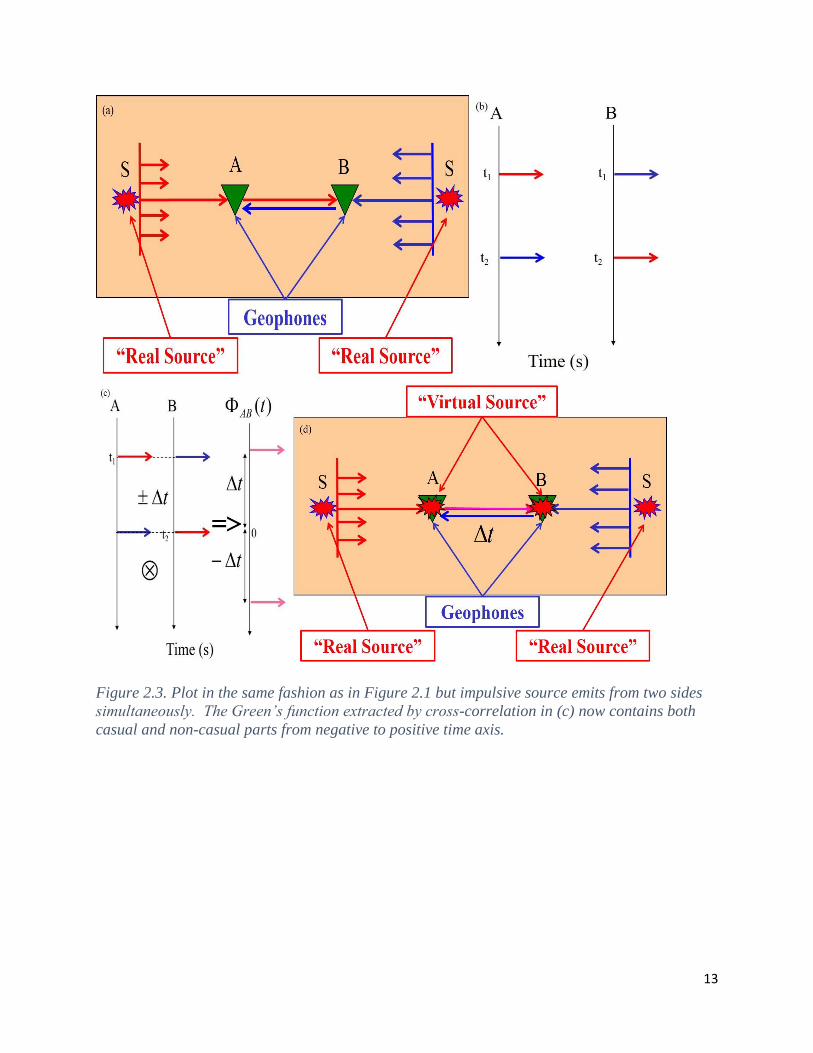
13

Figure 2.3. Plot in the same fashion as in Figure 2.1 but impulsive source emits from two sides

simultaneously. The Green’s function extracted by cross-correlation in (c) now contains both

casual and non-casual parts from negative to positive time axis.

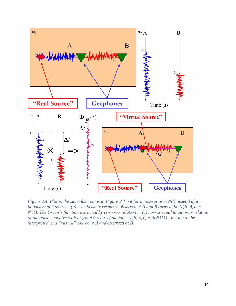
14

Figure 2.4. Plot in the same fashion as in Figure 2.1 but for a noise source N(t) instead of a

impulsive unit source. (b). The Seismic response observed at A and B turns to be . The Green’s function extracted by cross-correlation in (c) now is equal to auto-correlation

of the noise convolve with original Green’s function - . It still can be

interpreted as a “virtual” source at A and observed at B.

15

, simplifying to,

( ) ( ) ∑ (2.5)

This last expression indicates that the cross-correlation of seismic responses observed at two

stations, A and B, each of which is the stack of rightward and leftward propagating noise fields,

can extract the Green’s function, including both the casual and anti-causal parts, between the two

receivers A and B, convolved with the auto-correlation of the source function.

Wapenaar, et al. (2010) summarized three key conclusions regarding this simple 1D

analysis of direct-wave interferometry. First, we understand interferometry works in both cases:

transient source as well as noise sources. This feature originates and distinguishes two dominant

applications of seismic interferometry, namely passive seismic interferometry, and exploration

seismic interferometry. In the case of exploration seismic interferometry, the responses of

impulsive or transient sources must be cross-correlated separately, and follow a summation over

sources. In the case of passive seismic interferometry, a single cross-correlation over all

response records is sufficient, despite information related to sources. Secondly, an isotropic

illumination of the receivers is required to obtain a time-symmetric causal and anti-causal

response of Green’s function between the receivers. Equal illumination means a balanced right

and left side sources in 1D case, but we will address this task much more specifically in 2D/3D

analysis of direct-wave interferometry in terms of a more complex geometry. Thirdly, in the real

world, we always encounter the antisymmetric Green’s function over time zero axis rather than

time-symmetric case due to variations in source distribution from case to case (Grechka and

Zhao., 2012, Zhao and Rector., 2011). I present applications of noise datasets in Chapter 3 and

Chapter 4.

2.3 2D and 3D Passive Wave Interferometry

It is time to extend the analysis to 2D and 3D direct wave interferometry. To illustrate

several numerical synthetic examples are provided. Figure 2.5(a) considers a simple 2D

configuration, acoustic lossless medium, and two geophone receivers separated by 200m. The

background wave velocity is 2000 m/s, a circle of transient sources is distributed uniformly,

emitting at a central frequency of 50 Hz, denoted by red explosive polygon. The angle between

every two sources on this circle is about 10 degrees and the distances to each receiver ranges

from 200m to 400m. Figure 2.5(b) and (c) displays the angle gather collected at the two

receivers, shown as a function of polar source coordinate (angle) and travel time (ms). Repeating

the same procedure for the 1D interferometry of an exploration transient source, we simply

cross-correlate these two angle gathers for each source (trace) separately. The cross-correlation

gather remains a function of polar source coordinate smoothly varied with travel time but with an

auto-correlation of source wavelet A(S(t)) instead of S(t) , as shown in Figure 2.6(b), since the

cross-correlation cancels everything out leaving only the travel time difference along the paths

between the two receivers .

16

Figure 2.5. Cartoon Example of 2D direct wave interferometry. (a) Impulsive responses

generated by a 360 degree circle of uniform distributed source propagating from outside to

inside. (b)(c) Angle gather plot of responses at two receivers – green functions G (S, A, t) and G

(S, B, t) in polar coordinates from -90 to 270 degree.

17

Figure 2.6. (a) Impulsive responses generated by a 360 degree circle of uniform distributed

source, red dashed lines indicated Fresnel zones along the receiver line, (b)Cross-correlation of

the two angle gathers recorded in Figure 2.5 (b) (c), red dashed lines indicated Fresnel zones.

(c) Stack the correlation gather in (b). This can be represented by ( )*A(S(t)), Green’s function mainly contributed from sources inside Fresnel zones, the

rest sources cancel each other out.

18

Comparing the 2D case with the examples of 1D direct wave seismic interferometry, the

left hand side response generated by the source at angle zero is equal to the plane-wave source at

S in Figure 2.1. Similary, the right hand side response generated by the source at angle 180

plays the same role as the plane wave transite source shown in Figure 2.2. The arrivial times are

. If we stack over all traces in the correlation

gather in Figure 2.6(b), and then we obtain a time-sysmmetric response in Figure 2.6(c), which is

again an auto-correlation of source wavelet convolve with both casual and anti-causal Green’s

function, may written as ( ) ( ) similar to equation 2.5.

Several interesting phenomenon are observed from the 2D direct wave seismic

interferometry. Instead of the implusive source in 1D analysis, we encouter sources with finite

frequency content, which leads to not only the sources falling exactly at zero angle and 180

degree angle contributing to the final Green’s function represented in Figure 2.6(c), but also

includes contributions from sources along the horizontal axis inside the Fresnel zones, as

highlighted by the red dashed lines shown in Figure 2.6(a)(b). This is because these sources have

stationary phase on the travel time curve, and then interfere constructively, and stack coherently

from the cross-correlation gather. Conversely, the events outside the Fresnel zones interfere

destructively, and give no coherent contribution to the Green’s function, given a uniform

distribution of such sources those located outside the Fresnel zones cross-correlate to zero.

There is a small noise wavelet at time zero in Figure 2.6(c), which occurs because there is an

imperfect distribution of sources which leads to an imperfect travel time curve.

Repeating the same procedure as demonstrated for the 1D direct wave interferometry

analysis, instead of stacking the contributions from transient sources we can extend the source

function to be noise sources. Figure 2.7 shows the same geometry as Figure 2.5 but the responses

generated by a band-limited random noise source N(t) emitting continually and simultaneously.

(only 24 traces shown for display purpose; the relative arrival times from each source at the

circle to receiver are labelled by the red dash lines). Assuming that the noise are uncorrelated, a

single cross-correlation and stacking over all traces creates the response between the two

receivers equivalent to the Green’s function convolving with auto-correlation of the noise. The

final expression is analogous to equation (2.5) ( ) ( )

, where ( ) .

19

Figure 2.7. Plot in the same fashion as in Figure 2.5 but for a noise source N(t) which emits

continually and simultaneously. (b)(c) The noise angle gather observed at the two receivers. The

relative arrival times of noise sources are labelled by the red dash lines.

20

Figure 2.8. Plot in the same fashion as in Figure 2.6 but (a) Seismic responses generated by a

360 degree circle of noise source N(t) instead of impulsive unit sources., red dashed lines

indicated Fresnel zones along the receiver line, (b)Cross-correlation of the two angle gathers

recorded in Figure 2.7 (b) (c), red dashed lines indicated Fresnel zones. (c) Stack the correlation

gather in (b). This can be represented by ( ) * A(N(t)), where A(N(t))

stands for auto-correlation of noise signals.

21

Several features are observed in this analysis. First, the symmetry of the response still

relies on the isostropic illumination of the receivers. Second, the final cross-correlation response

we obtained as shown in Figure 2.8(c) appears to have a much lower S/N ratio than in the

previous 2D example, which leads to it being shaped as a wavelet rather than a perfect delta

function. This is primarily caused by the frequency band-limited sources, plus an insufficient

density of azimuthal coverage of sources due to limitations of computer memory.

Overall, these 2D example anaylses show that the important criterion for the distribution

of actual sources is to sourround the receivers of interest compleletely. Furthermore, the sources

are not necessarily primary sources but also can be secondary sources. (e.g. reflection points or

scatters). In the realistic earth, we always encounter the case with a complex, multilayered tilted

medium. A perfect source coverage is always available to implement interferometry since there

are sufficient secondary sources (e.g. free surface of the Earth, faults or internal scatters) in the

medium of interest (Andrew et al, 2006, Snieder et al, 2002). Naturally, we can extend our

seismic interferometry analysis from a 2D distribution of sources to a 3D distribution. The main

modification is that the sources must surround the medium entirely; the stacking or integrating

step is then performed over the cross-correlation from that entire set of sources, switching from

Fresnel zones to Fresnel volumes.

In the discussion above, the basic principles of seismic interferometry was introduced in a

heuristic way. That provided the sufficient theoretical basis for our study, since we focus on

generalization and variations of passive interferometry using microseismic, human cultural and

traffic noise for a variety of seismic applications. A number of pioneers have derived the passive

interferometry methodology in a formal mathematical way, that is, Green’s function extraction

from normal modes (Lobkis and Weaver, 2001; Campillo and Paul, 2003), Green’s function

representation theorems (Wapenaar, 2004; Wapenaar and Fokkema, 2006; Shapiro and Campillo,

2004. 2005), the principle of time reversal (Roux and Fink, 2003), and stationary phase analysis

(Snieder et al., 2006). After such processing, one receiver serves as a (virtual) source for waves

recorded by other receivers, which leads to a pseudoshot gather for many receivers, without

using an active source.

2.4 Interferometric computational methods

In the previous analysis of seismic interferometry, we focused on the retrieval of Green’s

function only by cross-correlation. In the past several years, several new interferometry

computational methods were proposed. The first proposed method is deconvolution

interferometry. In this method, the source signal is removed by means of spectral division. The

mathematical theory of deconvolution interferometry has been derived by Vasconcelos and

Snieder (2008a), and the multidimensional deconvolution method has been formulated for

seismic interferometry (Wapenaar et al., 2008a, 2008b). Nakata et al., 2010 used the cross-

coherence as the second method for shear wave imaging using traffic noise. They calculate the

cross-correlation of traces normalized by their spectral amplitudes in the frequency-domain.

Bensen et al. (2007) show examples of normalization techniques applied in seismic

interferometry. The third method developed in my work takes Nakata’s (Nakata et al., 2011)

cross-coherence method one step further by completely removing the amplitude information

22

from input data directly in time domain, replacing the traces with only the signal signs

maintaining phase information(Aki, 1957; Bendat and Piersol, 2000; Campillo and Paul, 2003;

Shapiro et al., 2005)

Snieder et al., 2009 summarized both the advantages and disadvantages of the various

methods. Cross-correlation is stable but needs estimation of the power spectrum of the noise

source and relatively sensitive to complicated waveforms. Deconvolution is potentially unstable

and, thus, needs regularization, but this method does not require estimation of the source

spectrum. Third, both cross-signs and cross-coherence methods have a way to extract the phase

of each trace but neglect the amplitude information. These methods all have strengths and

weaknesses, and we should choose the method that best suits the data.

2.4.1. Cross-correlation

Let’s first review the cross-correlation methods in a closed 3D space (Wapenaar and

Fokkema, 2006), which consists of the earth’s surface and an arbitrary shaped surface at depth

∑ | | ( ) (2.6)

Where the asterisk stands for convolution, | | is the average of the power spectrum for the

source wavelet, and still denotes seismic responses recorded at two receivers B and A,

and the Green’s function extracted between them. Recall that the extracted Green’s function is

mostly determined by sources at stationary phase locations. These sources launch waves that

propagate to the receiver B, and then continue to the receiver A. However, if we normalize input

traces prior to cross-correlating in equation (2.6) which can help suppress contributions of strong

bursts of energy. This renders the amplitude unreliable, but the phase is still correct, denoted as

equation (2.7)

∑

( )

( ) (2.7)

An example is shown in Figure 2.9, where uncorrelated random noise travels from stationary

source locations through receiver B to receiver A. The wave arrival time at B is 0.2s earlier than

it arrives at A. Each seismic record is normalized by its maximum values, which suppresses the

influence of strong amplitude events. The cross-correlation of the normalized records clearly

shows the phase difference of 0.2 s.

23

Figure 2.9. An example of normalized cross-correlation. Noise recorded at receiver B and A

from a stationary phase source locations. Seismic records normalized by its maximum value.

Cross-correlation of normalized records.

2.4.2 Cross-Sign

Larose et al. (2004), Bensen et al. (2005) suggested removing the amplitude information

from input data by replacing the traces with their signs described as equation 2.8, where

∑ ( ) (2.8)

The results of equation (2.8) is illustrated in Figure 2.10. It confirms the precise time difference

at 0.2s, same as Figure 2.9, with a slight amount of noise increased. Cross-sign deletes

amplitudes but is not harmful for the travel times. Comparison with a variety of microseismic

implementations between equation (2.7) and equation (2.9) is introduced in Chapter 3. The final

outcome shows the case and computations performed with the two equations can be deemed

identical for practical purposes.

24

Figure 2.10. An example of cross-signs, plot in the same fashion as Figure 2.9. Taking signs

(±1) of seismic records. Cross-correlation of the signs still deliver the precise time difference at

0.2s with a slight amount of noise added.

2.4.3 Deconvolution

Deconvolution interferometry is defined as

∑

| | , (2.9)

where is the power spectrum of Green’s function at receiver A. Deconvolution removes

the influence of the source wavelet . Because of the absolute value in the denominator, the

phase of is determined by the numerator ; hence, the deconvolution gives

the same phase as the cross-correlation and cross-sign methods. Because of the spectral division,

the result is independent of the source signature. The method can deal with data generated by

long and complicated source signals. (Vasconcelos and Snieder, 2008a)

2.4.4. Cross-Coherence

The cross-coherence is denoted as

∑

| || | , (2.10)

25

where the denominator and is the product of the power spectra of the two

waveforms recorded at receiver B and A. The numerator is same as the expression of cross-

correlation. Theoretically, cross-coherence cancels out the source wavelet by division as

well as discarding the amplitude information, and only maintains the phase information. The

method, similar to deconvolution method, can deal with data generated by long and complicated

source signals. (Nakata et al., 2010).

In the deconvolution and cross-coherence approach shown here, some level of white

noise has to be added to prevent numerical instability if the power spectrum of the seismic

records is minor in the denominators. If we choose a regularization parameter that is too large,

the regularized deconvolution reduces to cross-correlation. If, however, the regularization

parameter is too small, the deconvolution is unstable. Although instability also occurs in cross-

coherence, in practice in Chapter 3 and Chapter 4, we found cross-correlation (equation 2.8) and

cross-sign (equation 2.7) deliver us the best reliable and stable results in terms of fairly

straightforward source wavelets, inadequate frequency spectra and computational cost.

Figure 2.11 An example of deconvolution and cross-coherence method, plot in the same fashion

as Figure 2.9. The power spectrums of the records at A and B are shown. Cross-coherence

illustrates a lesser noise contamination compared to the deconvolution method.

26

2.5 Conclusion

I have heuristically discussed the basic principles of seismic interferometry, and have

shown that whether we consider controlled-source or passive interferometry, virtual sources are

created at positions where there are only receivers. Of course no new information is generated by

interferometry, but information hidden in noise or in a complex scattering noise, is reorganized

into easy interpretable responses that can be further processed by standard tomographic inversion

or reflection imaging methodologies. The main strength is that this “information unraveling”

neither requires knowledge of the medium propagation velocity or density nor of the location or

initial emitting time of the real sources. Moreover, we discussed several popular computational

methods of interferometric processing, including cross-correlations, cross-sign, deconvolution

and cross-coherence. In practice, which method is the best to use is almost entirely data-driven

on a case by case basis.

27

2.6 References Aki, K., 1957, Space and time spectra of stationary stochastic waves, with special reference to

microtremors.: Bull. of the Earthquake Res. Inst. Univ. Tokyo, 35, 415–456.

Bendat, Julius S., and Allan G. Piersol. "Random data analysis and measurement procedures."

Measurement Science and Technology 11.12 (2000): 1825.

Bensen, G. D., et al. "Processing seismic ambient noise data to obtain reliable broad‐band

surface wave dispersion measurements." Geophysical Journal International 169.3 (2007): 1239-

1260.

Bensen, G.D., Ritzwoller, M.H., Shapiro, N.M. & Levshin, A.L., 2005. Extending ambient noise

surface wave tomography to continental scales: application across the United States,EOS, Trans.

Am. geophys. Un., 86(52), Fall Meeting Suppl., Abstract S31A-0274

Campillo, Michel, and Anne Paul. "Long-range correlations in the diffuse seismic coda." Science

299.5606 (2003): 547-549.

Claerbout, Jon F. "Synthesis of a layered medium from its acoustic transmission

response." Geophysics 33.2 (1968): 264-269.

Curtis, Andrew, et al. "Seismic interferometry—Turning noise into signal." The Leading

Edge 25.9 (2006): 1082-1092.

Forghani, Farnoush, and Roel Snieder. "Underestimation of body waves and feasibility of

surface-wave reconstruction by seismic interferometry." The Leading Edge 29.7 (2010): 790-

794.

Larose, E., A. Derode, M. Campillo, and M. Fink, 2004, Imaging from one-bit correlations of

wideband diffuse wavefields: Journal of Applied Physics, 95, No. 12, 8393–8399.

Lobkis, Oleg I., and Richard L. Weaver. "On the emergence of the Green’s function in the

correlations of a diffuse field." The Journal of the Acoustical Society of America 110 (2001):

3011.

Miyazawa, M., R. Snieder, and A. Venkataraman, 2008, Application of seismic interferometry to

extract P- and S-wave propagation and observation of shear-wave splitting from noise data at

Cold Lake, Alberta, Canada: Geophysics, 73, No. 4, D35–D40.

Nakata, Norimitsu, et al. "Shear wave imaging from traffic noise using seismic interferometry by

cross-coherence." Geophysics 76.6 (2011): SA97-SA106.

Nowack, Robert L. "Seismic interferometry and estimation of the Green’s function using

Gaussian beams." Earthquake Science 23.5 (2010): 417-424.

O’Connell, Daniel RH, and James P. Turner. "Interferometric multichannel analysis of surface

waves (IMASW)." Bulletin of the Seismological Society of America 101.5 (2011): 2122-2141.

28

Roux, Philippe, and Mathias Fink. "Green’s function estimation using secondary sources in a

shallow water environment." The Journal of the Acoustical Society of America 113 (2003):

1406.

Schuster, G. T., 2009, Seismic Interferometry, Cambridge University Press.

Shapiro, Nikolai M., et al. "High-resolution surface-wave tomography from ambient seismic

noise." Science 307.5715 (2005): 1615-1618.

Snieder, Roel, et al. "A comparison of strategies for seismic interferometry."Surveys in

Geophysics 30.4 (2009): 503-523.

Snieder, Roel, et al. "Coda wave interferometry for estimating nonlinear behavior in seismic

velocity." Science 295.5563 (2002): 2253-2255.

Snieder, Roel, Kees Wapenaar, and Ken Larner. "Spurious multiples in seismic interferometry of

primaries." Geophysics 71.4 (2006): SI111-SI124.

Vasconcelos, Ivan, and Roel Snieder. "Interferometry by deconvolution: Part 1—Theory for

acoustic waves and numerical examples." Geophysics 73.3 (2008): S115-S128.

Wapenaar, K., D. Draganov, and J. O. A. Robertsson, 2008, Seismic Interferometry: History and

Present Status: SEG Geophysics Reprint Series, No. 26.

Wapenaar, Kees, and Jacob Fokkema. "Green's function representations for seismic

interferometry." Geophysics 71.4 (2006): SI33-SI46.

Wapenaar, Kees, et al. "Tutorial on seismic interferometry: Part 1—Basic principles and

applications." Geophysics 75.5 (2010): 75A195-75A209.

Wapenaar, Kees, et al. "Tutorial on seismic interferometry: Part 2—Underlying theory and new

advances." Geophysics 75.5 (2010): 75A211-75A227.

Wapenaar, Kees, Evert Slob, and Roel Snieder. "Seismic and electromagnetic controlled‐source

interferometry in dissipative media." Geophysical Prospecting56.3 (2008): 419-434.

Wapenaar, Kees, Joost van der Neut, and Elmer Ruigrok. "Passive seismic interferometry by

multidimensional deconvolution." Geophysics 73.6 (2008): A51-A56.

Wapenaar, Kees. "Green's function retrieval by cross‐correlation in case of one‐sided

illumination." Geophysical Research Letters 33.19 (2006).

Weaver, Richard L., and Oleg I. Lobkis. "Ultrasonics without a source: Thermal fluctuation

correlations at MHz frequencies." Physical Review Letters87.13 (2001): 134301.

Yao, Huajian, and Robert D. Van Der Hilst. "Analysis of ambient noise energy distribution and

phase velocity bias in ambient noise tomography, with application to SE Tibet." Geophysical

Journal International 179.2 (2009): 1113-1132.

Zhan, Zhongwen, and Sidao Ni. "Stationary phase approximation in the ambient noise method

revisited." Earthquake Science 23.5 (2010): 425-431.

29

30

Chapter 3

Microseismic interferometry

3.1 Summary

This chapter demonstrates the useful application of seismic interferometry using noise,

which would be usually discarded, to determine useful information for velocity model

construction as well as defining local structural parameters, such as P- and S-wave velocities and

a shear-wave-splitting coefficient. Importantly, natural sources of noise appear to possess wide

spatial apertures, allowing the successful reconstruction of waves that travel directly between the

downhole receivers. As previously stated in Chapter 2, an important application of passive

seismic interferometry is to retrieve Green’s function of the body waves between the downhole

receivers from the microseismic noise, we called it “microseismic interferometry”. Instead of the

widely used applications on the retrieval of seismic surface between seismometers and the

subsequent tomographic determination of the subsurface wave velocity distribution using the

earth ambient noise, we present the results of interferometry applied to a number of passive

downhole microseismic data sets acquired in the hydrocarbon-bearing Niobrara, Eagle Ford, and

Bakken formations from Wyoming, British Columbia, Texas, North Dakota and Colorado.

Although the available three-component (3C) data make it theoretically possible to recover full

elastic Green’s tensors for any receiver pair, we choose to restrict the scope of our study to a

single, along-the-well component of the three-component (3C) records. Depending on the survey

geometry, cross-correlations of this component retrieve either P- or S-waves traveling between

the receivers and allowing one to estimate the velocities useful for building models for

microseismic data processing. We perform shear wave-splitting anisotropy analysis from these

microseismic datasets. The direction of polarization of the fast S-wave datasets from Goundbrich,

British Columbia and Magnolia, Texas is in agreement with the clouds of the microseismicity,

and the direction of the maximum principal stress.

3.2 Introduction

The past decade witnessed rapid development of the theory of seismic interferometry

followed by numerous applications of interferometric approaches in seismic exploration and

exploitation. This body of work, partially collected in the Seismic Interferometry supplement of

Geophysics (2006), SEG reprint volume (Wapenaar et al., 2008), and the Interferometry

Applications special section of The Leading Edge (2011), conclusively demonstrates that a stack

of cross-correlations of traces recorded by two receivers over sources appropriately distributed in

three-dimensional heterogeneous earth can retrieve a signal that would be observed at one

receiver if another acted as a source of seismic waves. This assertion is applicable to both active-

source data (many instructive geometries of this kind are examined by Schuster, 2009) and

passive records of ambient noise; examples of the latter, summarized by Snieder and Wapenaar

(2010), range from ultrasonics (Weaver and Lobkis, 2001) to global seismology (Shapiro et al.,

2005).

Passive seismic interferometry, sometimes called stochastic interferometry, is especially

well suited for downhole microseismic applications. Microseismic monitoring of hydraulic

31

stimulations of low-permeability reservoirs typically lasts for days, supplying abundant data for

turning geophones into virtual sources (in the terminology of Bakulin and Calvert, 2004) and

analyzing the obtained outputs. To the best of our knowledge, this opportunity was first

recognized by Miyazawa et al. (2008), who reconstructed the body P- and S-waves propagating

along a wellbore from steam-injection noise recorded by 3C receivers. Essentially, we follow

their footsteps but with two modifications that appear to be important in practice. First, we can

retrieve meaningful, clean, and straightforwardly interpretable signals from cross-correlations of

minutes of passive data as opposed to a month-long record employed by Miyazawa et al. (2008).

Second, we do not explicitly remove locatable microseismic events from the cross-correlation

process and, instead, let normalization and stacking smooth out the associated amplitude

anomalies.

In what follows, we describe the results of interferometry applied to a number of

downhole microseismic data sets acquired in the hydrocarbon-bearing Niobrara, Eagle Ford, and

Bakken formations from Wyoming, British Columbia, Texas, North Dakota and Colorado.

Although the available 3C data make it theoretically possible to recover full elastic Green’s

tensors for any receiver pair, we restrict the scope of this chapter to single, along-the-well

component of our 3C records. Depending on the survey geometry, cross-correlations of this

component yield either P- or S-waves traveling between the receivers and allowing one to

estimate the associated velocities that can be used to build models for microseismic data

processing.

3.3 The Geology

This chapter we processed a number of downhole microseismic data sets acquired by

Marathon oil company and Shell exploration & production company, in the hydrocarbon-bearing

Niobrara, Eagle Ford, and Bakken formations from Pinedale Wyoming, Groundbirch British

Columbia, Magnolia Texas, North Dakota and Colorado. These areas cover a large percent of

current unconventional shale gas plays in north America, as illustrated in Figure 3.1. No further

information of the operational site geology is addressed without releasing permission from

Marathon and Shell, we only discuss the general background of several shale formation used in

the study.

The Niobrara Formation also called the Niobrara Chalk, is a geologic formation on the

east slope of the Rocky Mountains that was laid down between 87 and 82 million years ago

during the Coniacian, Santonian, and Campanian ages of the Late Cretaceous. It is composed of

two structural units, the Smoky Hill Chalk Member overlying the Fort Hays Limestone Member.

The chalk formed from the accumulation of coccoliths from microorganisms living in what was

once the Western Interior Seaway, an inland sea that divided the continent of North America

during much of the Cretaceous. In the eastern basins of Colorado, deposits include chalk (made

predominantly from algae-derived carbonate plates known as coccoliths), carbonate mud, shale,

and silt. In the western basins, less chalk is present, with instead more shale, silt, and sand that

was shed from the rising mountains to the west. Here the Niobrara is often grouped as part of the

Mancos Shale Formation. The overall thickness of the Niobrara Formation varies between 200

and 400 feet in northeastern Colorado. In northwestern Colorado, however, thicknesses can be

much greater—in places more than 1500 feet.

32

Figure 3.1. Shale Plays in North America (source: U.S. Energy information administration)

The Bakken formation is a rock unit from the Late Devonian to Early Mississippian age

occupying about 200,000 square miles of the subsurface of the Williston Basin, underlying parts

of Montana, North Dakota, and Saskatchewan. The formation is entirely in the subsurface, and

has no surface outcrop. The rock formation consists of three members: lower shale, middle

dolomite, and upper shale. The shales were deposited in relatively deep anoxic marine conditions,

and the dolomite was deposited as a coastal carbonate bank during a time of shallower, well-

oxygenated water. The middle dolomite member is the principal oil reservoir, roughly two miles

below the surface. Both the upper and lower shale members are organic-rich marine shale.

Porosities in the Bakken average about 5%, and permeabilities are very low, averaging 0.04

millidarcies—much lower than typical oil reservoirs.

The Eagle Ford Formation is a sedimentary rock formation from the Late Cretaceous age

underlying much of South and East Texas in United States, consisting of organic matter-rich

fossiliferous marine shale. It derives its name from the old community of Eagle Ford, now a

neighborhood in West Dallas, where outcrops of the Eagle Ford Shale were first observed. Such

outcrops can be seen in the geology of the Dallas–Fort Worth Metroplex . The formation is the

source rock for the Austin Chalk oil and gas formation. The formation’s carbonate content can

be as high as 70%. The play is shallower and the shale content increases in the northwest

33

portions of the play. The high carbonate content and subsequently lower clay content make the

Eagle Ford more brittle and easier to stimulate through hydraulic fracturing or fracking. In

geological terms, the Eagle Ford dips toward the Gulf of Mexico.

3.4 Computations

We begin with outlining our computational procedure that was performed in the time, ,

domain. Let be the normalized, along-the-well component of 3C seismic trace that

belongs to the shot gather and is recorded by the receiver . Our usage of the term “receiver” is

conventional because we know where receiver is located and what it records; the term “shot

gather,” however, needs to be explained. Since passive data, such as those displayed in Figure

3.2, contain waves arriving from unknown natural sources to our receivers in a selected time

interval , we define a shot gather as data recorded by the receiver string during that time

interval. According to the adopted definition, Figure 3.2 shows one second long ( 1 s) shot

gather.

Figure 3.2. Randomly chosen 1 s long microseismic shot gather recorded by a string of 10

downhole receivers. This gather represents typical input data for the case studies discussed in

the paper.

We take two traces and of shot gather recorded at and and cross-

correlate them. We then stack the obtained cross-correlations over a subset of the available shot

gathers. The spectrum of the result,

34

∑ ∑

, (3.1)

where denotes the time lag, is proportional to the sum of spectra of the causal and acausal

band-limited Green’s functions between and if the physical sources (for instance,

contributing to the gather in Figure 3.1) have random and uncorrelated spatial locations and

amplitudes (Weaver and Lobkis, 2001).

A few operational comments are now in order.

3.4.1 We normalize traces prior to cross-correlating them to suppress contributions of strong

bursts of energy (e.g., microseismic events) whose signal-to-noise ratios can reach over 100.

Although we find this type of normalization convenient because it eliminates the need to

establish a threshold for ambient noise and filter the input data accordingly, such an equalization

of amplitudes is not absolutely critical. The reason for its unimportance appears to be a

significant violation of the assumption of randomness of natural seismic sources (Weaver and

Lobkis, 2006), the violation that prevents one from retrieving the correct amplitudes of waves

comprising (equation 3.1). If the true amplitudes of waves are unrecoverable in our conditions

and obtaining the correct kinematics remains the only realistically achievable goal, amplitudes of

input traces can be severely distorted without compromising the travel time information (see

Figures 9 and 10 below).

3.4.2. The time interval defining the length of a shot gather is a free parameter that needs to be

selected. After experimenting with intervals ranging from 0.5 s to 15 s, we found that a particular

value of has little influence on the final result, that is, on travel times of the expected arrivals,

as long as is several times greater than the length of the maximum cross-correlation time lag .

3.4.3. We apply zero-phase bandpass filters to the produced stacks of cross-correlations to

enhance their visual appearance. The frequency bandwidths of our filters, listed in the Figure

captions, are sufficient to preserve useful information in each displayed interferometric output.

3.5 Synthetics Study

Similar to the passive seismic geometry of 2D configuration introduced in Chapter 2, we

consider using 2D ray tracing instead of full waveform modeling. Figure 3.3(a) considers a

simple 2D configuration, acoustic lossless medium, and two downhole 3C geophones A and B

apart vertically 500m from each other. The background velocity is 1750 m/s, a line of band-

limited random noise source N(t) emitting continually and simultaneously on the surface,

denoted by the red circles. The receivers were buried in the depth of 350m and 850m,

respectively. The arrivals of the direct-waves are labeled by the red dash lines. Assume that the

noise are uncorrelated, a single cross-correlation of stacking all traces creates the response

between the two receivers equivalent to the Green’s function convolving with auto-correlation of

the noise. The cross-correlation cancels the influences along the mutual ray path, but maintains

travel time difference between the two receivers. The final expression is analogous to equation

(2.5) ( ) ( ) , where

( ) , as demonstrated in Figure 3.2(d)(e). Recalling section 2.2 from Chapter 2, the

symmetry of the response still relies on the isotropic illumination of the receivers. Given the

35

band-limited frequency of the one-side passive sources plus less coverage of the source

distribution, it only recovers the casual part of the Green’s function (positive axis), which is

shaped like a wavelet rather than a perfect delta function.

36

Figure 3.3. Synthetic example of microseismic interferometry. (a) The seismic responses

generated by noise source N(t) which emits continually and simultaneously from surface to

downhole geophones. (b)(c) Receiver gather plot of the responses at two receivers A and B. The

arrival times of noise sources are labelled by the red dash lines. (d)Cross-correlation of the two

receiver gathers. (e) Stack the correlation gather in (d). This can be represented by ( ) * A(N(t)), where A(N(t)) stands for auto-correlation of noise signals.

3.6 Zero-offset VSP

Our first data set was acquired in a vertical well drilled to monitor hydraulic stimulation

of the Niobrara formation (Colorado, USA). In this geometry, as presented in Figure 3.4,

retrieving VSP (vertical seismic profiling) data from microseismic noise is possible. An example

of such zero-offset VSP is presented in Figure 3.5a, in which only 1 minute of raw record, whose

portion is displayed in Figure 3.2, sufficed to produce a meaningful output. As Figure 3.5a

demonstrates, turning the shallowest receiver into a source recovers a causal downgoing wave.

Since we cross-correlate the vertical along-the-well receiver components, it ought to be a P-

wave. Its nature as the body P-wave propagating in rocks surrounding the borehole becomes

clear once we compare its travel times with those (red dots in Figure 3.5a) derived from a sonic

log (Figure 3.5b) in a nearby vertical well. Sources of noise generating the P-wave in Figure 3.5a

have to be located above the receivers and likely relate to human activity on the well pad.

37

Figure 3.4. Geometry of the downhole observation well. Along the observation well, 42

geophones, indicated by black triangles, are installed at depths from 1300m to 2000m to monitor

the induced microseismicity. The area of stationary phase directly above the well.

Let us note that another, arbitrarily chosen minute of data would not yield exactly the

output shown in Figure 3.5a because natural sources are distributed nonuniformly in space and

nonperiodic in time. Their spatial nonuniformity is evidenced by the absence of upgoing waves

in Figure 3.5a and the lack of their temporal periodicity – by our inability to find two sets of

different shot gathers resulting in the same stack. Still, all examined stacks exhibit P-waves

similar to the one in Figure 3.5a and make the differences in their propagation times a useful

measure of the uncertainty in reconstructing kinematics of VSP-type data from microseismic

noise.

38

Figure 3.5. (a) Zero-offset VSP retrieved from 1 minute of microseismic data (T= 15 s, f= [10,

50] Hz) recorded above the Niobrara formation. The red dots in (a) indicate the times obtained

by integrating the P-wave sonic log in (b).

The same procedures were applied to three more datasets acquired in similar vertical

wells drilled to monitor hydraulic stimulation of Eagle Ford and Bakken formations from

Pinedale Wyoming, Groundbirch British Columbia, Magnolia Texas. Figure 3.6a produce a

meaningful output of retrieving VSP data from Microseismic in Pinedale Wyoming. Dissimilar

to the Niobrara example, we turning the deepest receiver into a virtual source recovers an anti-

causal downgoing P wave, with stacking 16 minutes of raw record in the vertical along-the-well

receiver components. A zero-offset VSP survey (25 Hz Ricker wavelet) was conducted in field,

shown as the red traces on the top of retrieving VSP data colored in black traces in Figure 3.6a.

The reconstructed body P-wave (black traces) propagating in rocks surrounding the borehole

agree with the real VSP survey and travel times (red dots in Figure 3.6a) derived by the sonic log

(blue lines in Figure 3.6b) recorded nearby. Figure 3.6b illustrates a further comparison between

the sonic log and the interval velocities derived from the reconstructed and real VSP (black/red

stairs) by averaging the travel times of every 4 out of 16 receivers. The same as the previous

39

example, noise sources in Figure 3.6a directly located above the receivers, and likely relate to

human activity on the well pad. Note that the figures are no longer displayed in a manner of

variable density area but in simple wiggles for the display purpose of trace comparison between

reconstructed and observed datasets.

Figure 3.6(a) Zero-offset reconstructed VSP (black traces) retrieved from 16 minute of

microseismic data (T= 15 s, f= [10, 50] Hz) display against the real zero-offset VSP(red traces)

in field from Pinedale, Wyoming. The red dots in (a) indicate the times obtained by integrating

the P-wave sonic log in (b). (b) P-wave sonic log (blue line) along with the reconstructed P-

wave vertical velocity (black line), and the real P-wave velocity (red line). The reconstructed

wave indicates a strong agreement with other two in-field measurements.

Figure 3.7 (a) plot in the same fashion as Figure 3.6(a), shows a retrieving VSP data from

Groundbirch, British Columbia but turning receiver 24 (an array of 36 receivers) into a source

recovers a downgoing P wave. In addition to Figure 3.5(a) and Figure 3.6(a), Figure 3.7(a)

reveals both upgoing/downgoing tube waves caused by a bridge plug (attached to the deepest

geophone) at 2.830km. It measures as the P-wave propagating in drilling muds about 1600 m/s.

(b)

40

Figure 3.7. Plot in the same fashion as Figure 3.5. Zero-offset VSP retrieved from Microseismic

recorded in Goundbirch, BC. Strong tube waves observed in (a). The reconstructed wave

indicates a robust agreement with other two measurements despite interference from tube waves.

The fourth example comes from an array of ten receivers located in a vertical borehole

acquired in the Eagle Ford formation in Magnolia, TX, as summarized in Figure 3.8.

(b)

41

Figure 3.8. Plot in the same fashion as Figure 3.5. Zero-offset VSP retrieved from Microseismic

recorded in Magnolia, TX.

3.7 Direct measurement of the horizontal velocity

Our success in recovering the VSP in Figure 3.5a to Figure 3.8a suggests the possibility

of repeating the same process for receivers placed in a horizontal well. This sort of

interferometric reconstruction was attempted with microseismic data acquired in the Eagle Ford

(Texas, USA) by an array of eight receivers located in approximately horizontal section of a

deviated borehole (Figure 3.9). A stack of cross-correlations of 16 minutes of data retrieves an

arrival displayed in Figure 3.10. This is an acausal wave propagating along the well from its toe

towards its heel as indicated by the arrow in Figure 3.10. To excite this wave, noise sources

should be in or around the Eagle Ford formation to the south-east from the receivers. The

existence of such sources seems plausible because our receivers monitored hydraulic treatments

of a well located to the south-east from the receivers and recorded several hundred locatable

microseismic events (not shown).

(b)

42

Figure 3.9. Well trajectory (gray) and locations of receivers (triangles). The dip of the lateral

section covered by the receivers is 3°. The arrow points in the direction of propagation of the P-

wave reconstructed in Figure 3.9.

Approximating the moveout of the dominant phase in Figure 3.10 with a straight line

yields the average apparent velocity of 4.5 km/s. This approximately horizontal velocity is to be

compared with the sonic log in Figure 3.11 that exhibits the vertical velocity of about 4.1 km/s in

the depth interval covered by the receivers. If we disregard the difference in frequencies of

microseismic and sonic data and attribute the difference in the vertical and horizontal velocities

to anisotropy under the assumption that a vertically transversely isotropic (VTI) model is

appropriate for the Eagle Ford shales, our two velocities result in Thomsen (1986) anisotropy

coefficient ϵ of approximately 0.1. While ϵ is notoriously difficult to measure from the P-wave

surface reflection data, here we estimated it from passively recorded microseismic at no

additional data-acquisition cost. Clearly, the recovered value of ϵ can be used in a velocity model

constructed to locate the microseismicity.

43

Figure 3.10. Wave retrieved from cross-correlations of 16 minutes of data (T= 15 s, f= [20, 150]

Hz) that propagates in the direction of the arrow along the receiver string shown in Figure 3.8.

The slope of the dashed straight line implies the average apparent velocity of 4.5 km/s.

44

Figure 3.11. Sonic log in a vertical well indicating the P-wave velocity of about 4.1 km/s in the

depth interval covered by the receivers (triangles) in Figure 3.8.

3. 8 Shear-wave cross-well survey

Our next example comes from a dual-well microseismic survey (Figure 3.12) conducted

in the Bakken (North Dakota, USA). When we cross-correlate the vertical components of

receivers in well 1 with those in well 2 and stack the cross-correlations, we expect to retrieve the

shear (SV) waves propagating from one well to another. Turning receivers in well 2 into sources

yields the stacks of cross-correlations presented in Figure 3.13. To create the causal arrivals

observed in Figure 3.12, natural sources have to be located to the west from well 2 (Figure 3.12).

This time, we lack a hypothesis explaining their physical origin because hydraulically stimulated

wells monitored from wells 1 and 2 were located to the east from well 1 (not shown).

45

Figure 3.12. Geometry of dual-well microseismic monitoring in the Bakken. The locations of

receivers in two nearly vertical wells are marked with the triangles.

The absence of knowledge of the sources of natural noise does not prevent us from

picking the travel times of the main phase on seismograms in Figure 3.13 (red dots) and on

seismograms of other receivers in well 2 that also were turned into sources. Those time picks

yield a travel time cross-plot presented in Figure 3.14a. This cross-plot, exhibiting a sharp time

increase and, hence, a pronounced velocity reduction at a depth of about 3200 m in well 1, could

constitute an input to the cross-well travel time tomography. Instead of performing a full-scale

tomographic inversion, we extract the zero-offset times (that is, the times between receivers in

wells 1 and 2 that have the same depths) marked with the white line in Figure 3.14a and,

knowing the distances between the receivers in the two wells, convert the obtained times into the

average velocities. The resulting depth velocity profile is shown with the thick blocky line in

Figure 3.14b. Overall, it matches the shear-wave sonic log (thin line), proving that interferometry

has extracted the shear-wave cross-well data from natural noise.

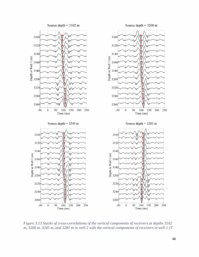
46

Figure 3.13 Stacks of cross-correlations of the vertical components of receivers at depths 3102

m, 3200 m, 3245 m, and 3281 m in well 2 with the vertical components of receivers in well 1 (T

47

= 0.5 s, f=[10, 100] Hz) The duration of the observation is 300 × 0.5 s = 150 s. The red dots are

the automatic time picks of the main retrieved phase.

The greatest velocity discrepancy between the sonic and the reconstructed velocity

profile, observed for the upper and lower Bakken shales (Figure 3.14b), relates to the resolution

of the retrieved cross-well data. As seismograms in Figure 3.13 indicate, the spectra of the cross-

well data peak at approximately 40 Hz, yielding the dominant shear wavelength of about 75 m.

At such a wavelength, the Bakken shale layers, whose thicknesses are 8 m and 15 m (Figure

3.14b), cannot be resolved individually and only contribute to a smooth velocity decline

exhibited by the recovered blocky profile.

Figure 3.14. (a) Travel time picks of the dominant phases, such as those in Figure 3.12, and (b)

shear-wave sonic log (thin line) along with the reconstructed S-wave vertical velocity (thick

blocky line). The white line in (a) indicates travel times extracted to calculate the blocky velocity

profile in (b). The triangles in (a) mark the locations of receivers in figure 3.6’s wells 1 and 2.

3. 9 Shear-wave splitting

It is known that a shear-wave propagating through rocks with stress-aligned micro-cracks

(also known as extensive dilatancy anisotropy or EDA-cracks) will split into two waves, a fast

one polarized parallel to the predominant crack direction, and a slow one, polarized

perpendicular to it. In the seismic case, the polarization direction of the fast split shear wave

parallels the strike of the predominant cracks regardless of its initial polarization at the source.

The differential time delay between the arrival of the fast and the slow shear waves (typically a

few tens of milliseconds) is proportional to crack density, or number of cracks per unit volume

within the rock body traversed by the seismic. Measuring the fast-shear wave polarization and

time delay from active source has thus become a valuable technique to detect the orientation of

local stress field.

48

Encourage from our successful reconstruction in retrieving P and S wave from 3.5(a) to

3.13(a), it is expected to observe interferometric shear-wave splitting from cross-correlations of

shear wave components recorded in the 3c receivers. We use the same microseismic data sets (16

mins, T= 15 s, f= [10, 50] Hz) acquired in a vertical well drilled to monitor hydraulic stimulation

of the GroundBirch, BC, as Figure 3.7(a) shows. Figure 3.15a reproduced two anti-causal shear

downgoing waves, as turning the deepest receiver into a source. Where the red/black traces

representing the two shear wave polarized to different angles. It’s achieved by rotating the two

horizontal components along-the-well receiver components from 0 to 180 degrees, and then

cross-correlate its horizontal components with an increment of 1 degree. The reconstructed

velocity of the body shear wave propagating around the borehole is convinced by comparing its

interval velocity (averaging travel times of every 4 receiver) to its shear sonic log (Figure 3.15b)

in a nearby vertical well.

49

Figure 3.15 (a) Zero-offset VSP retrieved of the fast(red traces) and slow(black traces) shear

waves from 16 minute of microseismic data (T= 15 s, f= [10, 50] Hz) recorded in Groundbirch,

BC. Auto-correlation of the fast/slow shear wave is identical to each other, in the case, the

red/black trace overlapping each other at the deepest receiver. (b) shear-wave sonic log (blue

line) along with the reconstructed S-wave vertical velocity (red line). (c) Zoom-in plot of cross-

correlations of fast (red traces) and slow (black traces) shear waves at the receiver #10. The

arrival time difference is about 2 ms.

50

Figure 3.15c demonstrates, the arrival of the black traces is slightly advanced by 2 ms

compared with that of the red traces. This means the shear wave polarized in the direction of the

black traces is faster than the shear wave polarized in the direction of the red traces, indicating

shear-wave splitting. The time delay between the fast/slow shear waves rises along with

augmented offsets, accordingly, the two shear waves overlapping each other in the case of its

auto-correlation in the bottom trace.

Figure 3.16. (a) Arrival times between receiver #10 and the bottom receiver as a function of

polarization angle. The black dots are measured arrival times. The outer circle indicates high

arrival times, and the inner circle indicates low arrival times. Shear wave polarized northeast –

southwest have higher velocities (low arrival times) than those polarized in other directions.

The values are approximately along N35E (fast) and S60E (slow), respectively. (b) Our receiver

array (black arrow) in the observation well sitting around by the microseismicity induced by

hydraulic stimulations of four treatment wells (red arrow). The microseismicity distribution,

mostly align with the maximum horizontal stress, is dominated by the values of N23.5E to N40E,

which agree with the polarization direction indicated by the fast shear wave in (a).

Figure 3.16(a) shows the retrieve shear-wave delay times as a function of polarization

angle. Black dots represent measured delay times. Shear wave polarized in the northeast

direction have less delay times (larger velocity) than polarized in other directions. The shear

wave splitting coefficient is about 2.1%. The development of linear trends of microseismicity

during hydraulic fracture stimulation treatments has been typically interpreted to be indicators of

the location of induced hydraulic fractures forming parallel to the maximum stress direction, as

51

displayed in Figure 3.16(b). Microseismicity reach an agreement with the direction of fast shear

wave polarized, approximately a value of N35E with acceptable error.

Another successful of shear wave splitting reconstruction is achieved to the microseismic

datasets (16 mins, T= 15 s, f= [10, 50] Hz) acquired in a hydraulic monitoring vertical well of the

Magnolia, TX, as Figure 3.8(a) shows. Figure 3.15a reproduced one causal shear downgoing

waves but turning the shallowest receiver into a source, where the black/red traces representing

the shear waves polarized to fast and slow direction. The shear wave velocity (blue dots in

Figure 3.17a) is evidenced by integrating the shear sonic log recorded nearby. Figure 3.17b is the

splitting delay times as a function of polarization angle. This case the shear wave polarized due

east-west have less delay times (faster velocity) than polarized in north-south. Figure 3.17(c)

demonstrates microseismicity triggered by the hydraulic stimulation of the treatment well (blue

line in Figure 3.17(c)) aligning with the polarization direction of the fast shear wave, as indicated

in 3.17(b).

Applications of shear-wave splitting analysis include monitoring changes of density and

orientation of fractures in subsurface media from continuous analyses. This can be useful to

monitor the reservoir and mitigate potential hazards during production. Further, this could

address challenges related to monitoring stress orientation and velocity changes along an active

seismic fault that may rupture in the future, including issuing warnings for volcanic eruptions

after noting structural changes associated with magma penetration.

52

Figure 3.17. Plot in the same fashion as Figure 3.16. (a) Zero-offset VSP retrieved of the fast

(black traces) and slow (red traces) shear waves from 30 minute of microseismic data (T= 15 s,

f= [10, 30] Hz) recorded in Magnolia, TX. . (b) Arrival times between the shallowest and the

deepest receiver as a function of polarization angle. Shear wave polarized due east – west have

higher velocities (low arrival times) than those polarized in other directions. The values are

approximately due east (fast) and north (fast), respectively. (c) A 3D view of our receiver array

deployed in the observation well (cyan line) sitting next to the treatment well (blue line). The

microseismicity distribution frequently arrange due east-west, which agree with the polarization

direction indicated by the fast shear wave in (a).

53

3.10 Concluding remarks and remaining issues

Interferometric processing of many passive data sets discussed in the chapter

demonstrates that noise, which would be usually discarded, contains information useful for

velocity-model construction. This information comes in the ability to retrieve various cross-well

and VSP-type data. Importantly, based on our experience, natural sources of noise appear to

possess wide spatial apertures, allowing the successful reconstruction of waves that travel

directly between the downhole receivers. While we can only speculate on the physical reasons

for those wide apertures, multiple scattering in the heterogeneous subsurface is likely to be one

of them.

We expect the number of applications of interferometry in microseismic to grow once

practitioners recognize its value and begin using the method. For instance, in addition to the

presented cross-well example, the P- and SH-wave cross-well data, similar to the SV-waves

displayed in Figure 3.10, could be recovered from cross-correlations of the horizontal

components of the original records, producing a full 3C cross-well data set that can be processed

using the available tomographic techniques. Another area of potential applications opens up if

receivers are left in place, enabling one to collect and analyze time-lapse data without the need

for employing active seismic sources.

54

Figure 3.18. Sign of data displayed in Figure 3.1.

Although many different applications can be envisaged, they all will have to deal with the

challenging issue of nonrandomness of natural sources that entails the apparent inability to

extract true amplitudes from interferometric reconstructions. However, if we embrace this

limitation as reality and aim at obtaining the correct kinematics, we get a surprisingly robust

methodology that depends on the wave amplitudes only weakly. To illustrate this point, we

follow the idea of Larose et al. (2004), who suggested that removing the amplitude information

from input data by replacing the traces with their signs (Figure 3.18) or equation 1 with

∑ ∑ sign

sign (2)

is not harmful for the travel times. Figure 3.19 shows that this is, indeed, the case and

computations performed with equations 1 and 2 can be deemed identical for practical purpose.

The results obtained so far leave us with a straightforward agenda: understand what

microseismic interferometry can provide, try to recover it, and learn from the experience.

55

Figure 3.19. Comparison of traces given by equations 1 and 2. The black traces, computed with

equation 1, are identical to those displayed in Figure 3.5a. The red traces were computed with

equation 2 for the same input data.

56

3.11 References

Bakulin, A., and R. Calvert, 2004, Virtual source: new method for imaging and 4D below

complex overburden: 74th Annual International Meeting, Society of Exploration Geophysicists,

Expanded Abstracts, 2477–2480.

Bakulin, Andrey, and Rodney Calvert. "The virtual source method: Theory and case

study." Geophysics 71.4 (2006): SI139-SI150.

Bakulin, Andrey, et al. "Virtual shear source makes shear waves with air guns."Geophysics 72.2

(2007): A7-A11.

Interferometry Applications Special Section, 2011, The Leading Edge, 30, No. 5 ,502–567.

Larose, E., A. Derode, M. Campillo, and M. Fink, 2004, Imaging from one-bit correlations of

wideband diffuse wavefields: Journal of Applied Physics, 95, No. 12, 8393–8399.

Miyazawa, M., R. Snieder, and A. Venkataraman, 2008, Application of seismic interferometry to

extract P- and S-wave propagation and observation of shear-wave splitting from noise data at

Cold Lake, Alberta, Canada: Geophysics, 73, No. 4, D35–D40.

Schuster, G. T., 2009, Seismic Interferometry, Cambridge University Press.

Seismic Interferometry Supplement, 2006, Geophysics, 71, No. 4, SI1–SI235.

Shapiro, N. M., M. Campillo, L. Stehly, and M. H. Ritzwoller, 2005, High-resolution surface

wave tomography from ambient seismic noise: Science, 307, 1615–1617.

Snieder, R., and K. Wapenaar, 2010, Imaging with ambient noise: Physics Today, 63, No. 9, 44–

49.

Thomsen, L., 1986, Weak elastic anisotropy: Geophysics, 51, 1954–1966.

Wapenaar, K., D. Draganov, and J. O. A. Robertsson, 2008, Seismic Interferometry: History and

Present Status: SEG Geophysics Reprint Series, No. 26.

Wapenaar, Kees, et al. "Tutorial on seismic interferometry: Part 1—Basic principles and

applications." Geophysics 75.5 (2010): 75A195-75A209.

Wapenaar, Kees, et al. "Tutorial on seismic interferometry: Part 2—Underlying theory and new

advances." Geophysics 75.5 (2010): 75A211-75A227.

Weaver, R. L., and O. I. Lobkis, 2001, Ultrasonics without a source: Thermal fluctuation

correlations at MHz frequencies: Physical Review Letters, 93, 254301-1–254301-4.

Weaver, R. L., and O. I. Lobkis, 2006, Diffuse fields in ultrasonics and seismology: Geophysics,

71, No. 4, SI5–SI9.

57

Wikipedia contributors. "Bakken formation." Wikipedia, The Free Encyclopedia. Wikipedia, The

Free Encyclopedia, 3 Mar. 2013. Web. 4 Mar. 2013.

Wikipedia contributors. "Eagle Ford Formation." Wikipedia, The Free Encyclopedia. Wikipedia,

The Free Encyclopedia, 18 Feb. 2013. Web. 4 Mar. 2013.

Wikipedia contributors. "Niobrara Formation." Wikipedia, The Free Encyclopedia. Wikipedia,

The Free Encyclopedia, 30 Oct. 2012. Web. 4 Mar. 2013.

58

Chapter 4

Using seismic surface waves generated by motor vehicles to

find voids: field results

4.1 Summary

In this chapter we present results based on several field experiments in which we study

seismic detection of voids using a passive array of surface geophones. The source of seismic

excitation is vehicle traffic on nearby roads, which we model as a continuous line source of

seismic energy. Our passive seismic technique is based on cross-correlation of surface

wavefields and studying the resulting power spectra, as previously stated in chapter 2, looking

for shadows caused by the scattering effect of a void. High frequency noise masks this effect in

the time domain, so it is difficult to see on conventional traces. Our technique does not rely on

phase distortions caused by small voids because they are generally too tiny to measure. Unlike

traditional impulsive seismic sources which generate coherent, broadband signals, ideal for

resolving phase but sometimes with insufficient energy, vehicle traffic affords a high energy

signal in a frequency range which is rich in surface waves. Field data results show that a septic

tank can be detected using traffic generated surface waves. From these results we conclude that

measuring scattered surface waves generated by motor vehicles could be a potentially useful tool

for finding underground voids.

4.2 Introduction

The detection of underground voids is an important application of geophysics. Tunnels and

bunkers are used to move people, drugs and weapons illegally across borders, and as bases for

terrorism. Forgotten tunnels collapse under the weight of drilling and earth-moving equipment

when they are exposed by open-pit mining. Houses are swallowed by historic mine workings

and sink holes (e.g. Blodgett and Kuipers, 2002).

In seismic interferometry, cross-correlations between two sensors can extract the Greens

functions between sensors using ambient noise as the energy source (e.g. Wapenaar, 2006;

Larose et al., 2006; Grechka and Zhao. 2012) which can provide an estimate of the subsurface

velocity structure, both using surface wave and body wave. In this paper, we suggest a low-cost,

reliable method of seismic interferometry for finding voids by measuring anomalies in amplitude

of seismic surface waves scattered by the voids.

Close to seventy percent of the energy from a seismic source at the surface propagates as

surface waves, mostly as Rayleigh waves (Park et al 1999). Rayleigh waves penetrate about a

wavelength into the earth, and can be scattered by structures that are buried about as deep as a

wavelength (Soccio and Strobbia, 2004). Different frequencies penetrate to different depths and

the so-called MASW method (Stokoe et al, 1994; Park et al., 2007) uses the dispersion curve

from Rayleigh waves to generate a velocity versus depth profile. However, many seismic

methods, including those designed to take advantage of surface waves, are optimized for

detecting small distortions in the time it takes seismic signals to travel between detectors

(geophones). The signals can be impulses generated by a point source such as a hammer

59

pounding on a steel plate (active seismic) or ambient noise (passive seismic and seismic

interferometry). The problem is that, although such techniques are ideal for finding the seismic

velocity of flat-lying geologic layers, small structures and voids only have a minimal impact on

seismic travel times, making them difficult to detect.

By contrast, surface wave amplitudes can be highly sensitive to near-surface scatterers.

Nasseri-Moghaddan (2006) used synthetic modeling to show that scattered energy gets

concentrated on the side of a void near a seismic source causing a bright spot and attenuated on

the other, causing a shadow. From this observation, he proposed a technique for the detection of

voids called Attenuation Analysis of Raleigh Waves (AARW). The depth of the void can be

inferred by the wavelengths affected by the shadow. He proposed using controlled sources with

energy concentrated in the surface wave frequency range.

When one thinks about using ambient noise as the source of surface wave energy, new

issues arise such as destructive interference of waves coming from different sources, the location

of sources, and the amplitude of a source itself. However, vehicle traffic is a well-constrained

source as cars and trucks are confined to traveling on mappable roads. If we can afford to sit and

average for a long time, we can think of the road itself as a line source of radiating energy. This

means that we can model what the geometrical effect of such a line source on our array of

geophones under hypothetical geologic conditions. We can also back out the distortions of the

earth out of the original signal and clean it up enough to discriminate between individual

vehicles.

Aki et al. (1957) acknowledged that most of the surface waves he studied in downtown

Tokyo were generated by traffic. Indeed, surface vibrations caused by cars and trucks are of

concern in historic building preservation (Kliukas et al, 2008). Hendricks (2002) compiled

results from over 20 vibration surveys conducted by the California Department of

Transportation. One of the main findings in these reports is that the bulk of the energy from

traffic-generated surface waves is in the 10-30 Hz range (except for some city buses which

wobble at frequencies well below 3Hz). At typical surface wave velocities of 200 to 500 m/s,

this makes cars and trucks an ideal source of energy for detecting voids buried 7 to 50 m deep.

In this chapter, we build a passive seismic method based on AARW concept, detecting tanks

based on measuring variations in the amplitude of seismic surface waves generated by motor

vehicles. Not only is the method inexpensive (it requires only a small set of off-the-shelf

geophones and a car), but it is simple to implement and the anomalies produced are easily

recognized.

4.3 Computations

Inheriting from a standard survey of passive seismic interferometry, a line of geophones is

set out near a suspected void. (We are still establishing geometrical limits of the method, but

60

intuition suggests that the geophones need to be within perhaps 10 wavelengths of the void.)

The geophones record for a period of time while a car drives along a road near or across the tank.

Traffic sources nearby target voids are treated as a radiating line energy source. At the end of the

period, each of the waveforms of vertical component recorded by the geophones is cross-

correlated with vertical waveforms recorded from the reference receiver.

The cross-correlation of displacement waveforms of traffic noise and in the

frequency domain are expressed as

*( , ) ( , ) ( , )AB A BC S D S D S (4.1)

Where C is the cross-correlation of two signs, and are the locations of geophone A and B,

respectively. is angular frequency; and * indicates a complex conjugate. Arbitrary cross-

correlations of vertical signals are stacked for the same sensor pair over all records to obtain the

average cross-correlation . Power spectra of the cross-correlations are then plotted as a

function of geophone position. We expect seismic voids scatter surface waves, resulting in a lack

of expected amplitude on the other, both of which can be easily measured.

4.4 Experimental Results

4.4.1 Modeling Results

All modeling was done using the 2-d mode of E3D, a 3D finite-difference elastic modeling

program developed by Shawn Larsen of LLNL. The program was used to validate our

experimental results by creating simulations based on the field setups at the locations of our field

experiments. The strategy for modeling roads at these locations employed a dense series of point

sources which is equivalent to a line source. The pattern of surface waves obtained as a surface

“snapshot” from E3D, match with the data we measured. Obviously, a single car driving along a

road is not a set of synchronized monochromatic seismic point sources. However, cars travel

slowly relative to surface waves; a car going at 20 mph is traveling about 9 meters/second

whereas a typical Raleigh wave velocity is at least 10 times faster, moving between 100 – 500

meters/second. This means that it is reasonable to assume that each individual in an ensemble of

traffic sits for a while and radiates at each point along the road. If we collect enough data and

average over time, we expect to be able to model the cumulative effect of passing cars as if the

road itself were radiating as a line source, or the sum of small, closely spaced point sources.

Figure 4.1a shows the geometry of a model of a tank buried in shallow surface. In this

simple model, a block shaped air filled tank was put in a background with a velocity typical of

alluvial gravels. The small blue square marks the x- position of the tank, as illustrated in Figure

4.1b, E3D returns a gather of vertical components of ground displacement. A geometrical

spreading correction of surface waves was applied to the shot gather and no additional

attenuation adding into the model. The effects of the tank are not easily visible at time domain

among all of the channels in a simulated seismic section. The same story as shown in Figure

4.1c, the phase shift due to the tank causes a slight perturbation in a plot of arrival time according

to geophone location, which has minimal impacts to phase region, making them difficult to

61

detect. Whereas in Figure 4.1d, an average power spectrum made by cross-correlating 17

geophones records with first geophone in frequency domain, arbitrarily normalized by the total

mean power, is plotted as a function of geophone location. There is a clearly visible build up of

scattered power on the side of the plot closest to the source, and a lack of amplitude (power

shadow) on the other, in a certain frequency range below 50Hz.

Figure 4.1(a): A 2-d model we used to illustrate the phase and amplitude effects of a tank on

seismic surface waves. All modeling was done using the 2-d mode of E3D, a finite-difference

elastic wave simulation code by Shawn Larsen of LLNL. In plots b, c and d, the small blue

square marks the x-axis position of the tank.

Tank

62

Figure 4.1(b): Shot gather from model geometry in Figure 4.1a. The effect of the tank is not

easily visible in a simulated seismic section. Geometrical spreading correction has applied to the

shot gather.

63

Figure 4.1(c): Travel times of first arrivals from shot gather in Figure 4.2a. The phase shift due

to the tank causes a slight perturbation in a plot of arrival time vs.geophone location.

Figure 4.1(d): In this plot, an average power spectrum, arbitrarily normalized by the total mean

power, is plotted as a function of geophone location. There is a clearly visible buildup of

scattered power on the side of the plot closest to the source, and a lack of amplitude on the other.

Power Shadow

Amplitude Buildup

Phase shift due to tank

64

4.4.2 First Field Experiment: seismic signal of cars

Our first field experiment was performed at the University of California, Richmond Field

Station at the intersection of two roads. A line of low frequency (4.5Hz) standard 24 geophones

with 20 ft spacing was set up to bisect angle between the two roads as shown in Figure 4.2a.

Figure 4.2b shows a typical spectrogram of the signal of a car driving along one of the roads.

The bulk of the signal is measured between 5-25 Hz. A freight train happened to pass on the

tracks during the acquisition. It appears as curved tones around 75 and 125 Hz in Figure 4.2b.

We conjecture that most of the energy comes from tires hitting small irregularities on the

pavement.

In a series of experiments, we acquired approximately a half hour of data with no cars

driving on the road (background), data with one car on a single road, and data with two cars

driving on the intersecting roads. In Figure 4.1c, we plot the average power spectrum for the

Two Car data sets as a function of receiver location minus that of the background. Since power

was measured in dB, the plots show an approximate signal/noise ratio. Figure 4 shows that most

of the signal was measured between 5 – 15 Hz. In Figure 4.1d, we extrapolate the s/n at 13 Hz

beyond the range of the survey to suggest that useful signal might be measured up to more than

200 m from the intersection of the roads. With a better array, more sensitive processing (such as

beam forming), and a longer averaging period, we expect that the range could be significantly

improved.

65

Figure 4.2(a): Field set up at the Richmond Field station. a) Google Earth image showing field

area, freeway and railroad tracks. b) Geophone layout. Experiments were performed with no

traffic, with one car idling at star location, with one car driving on one road and with two cars

driving on both roads.

Figure 4.2(b): Spectrogram (dB) shows the signal from a car (red colors are high amplitudes).

The signal (curved tones around 75 and 125 Hz) from a passing freight train was enormous

compared to the ambient noise. The maximum power in the signal is from 5 – 25 Hz.

Richmond Field StationRichmond Field Station

Tracks

Idling carIdling car

(a)

(b)

66

Figure 4.2(c): Mean power spectrograms (dB) of stacking all data sets as a function of receiver

distance after subtracting for background and ambient signal from Two Cars. Blue areas

indicate the regions where signal to noise ratio is negative. Orange and yellow areas indicate

the regions where there are enough signal to noise ratio.

67

Figure 4.2(d): An estimate of the signal to noise ratio indicates a range of approximately 250m

in 13Hz.

4.4.3 Second Field Experiment: Detection of a septic tank

We experimented with the detection of a shallow septic tank at the Glider Port in

Truckee. The tank is buried in an old glacial outwash plain, made up of small layers of cobbles,

gravel and sand. The top of the tank was about 1 ft below the surface. The bottom was about 12

ft. We placed a line of 24 geophones with 6' spacing along the dirt road so that we entirely

passed though the septic tank. We recorded about 28 minutes data consisting of 13 continuous

recording approximately each 130 second listening period. The field set up is shown in Figure

4.3a.

68

Figure 4.3(a): Experimental setup at Truckee Glider Port. Google Earth Satellite image showing

field area, road and septic tank, geophone layout. Geophones were set up along red line. Cars

were driven both along the dirt road shown as blue line, whch is perpendicular to the geophone

line. The top of the septic tank illustrated as yellow line, was about 2 ft below the surface. The

bottom is at about 12 ft.

Figure 4.3b shows preliminary results, a mean power-spectrum is displayed on a log scale as

a function of meters from the center of the septic tank. A car was driving on the road

perpendicular to the line of geophones from the north side. The x-axis gives lateral distance from

the center of the tank in meters. The y-axis measures frequency in Hz. The source was a car

driven at less than 10 mph on the dirt road perpendicular to the line of geophones. The mean

power spectrum map computed using a stack of cross-correlation of raw vertical waveforms with

reference to the receiver closest to road. A geometrical spreading correction of surface

waves was applied to focus power anomaly from the tank.

A significant attenuation was observed in amplitude of the mean power spectrum due to the

tank, because it is unnormalized (by the number of passes of the car along the road, signal

strength, recording interval, etc.) the spectrum anomaly should not be interpreted as any

particular physical quantity. The spectrum above 40Hz is absent by reason of unremitting air

wave contamination. In contrast, we didn’t observe an amplitude build-up on the road side of the

tank below, which may either be caused by large wavelengths skipping the shallow tank in terms

of its small size by given frequency range, or by insufficient traffic-induced signals filling the

fresnel zone caused by short recording times.

Traffic

Septic Tank

69

Figure 4.3(b): Evidence of the septic tank at Truckee, CA. A car was driven along the dirt road

nearby the tank and the mean power spectrum was computed after several passes of the car

along the road.

4.4.4 Third Experiment: railroad tunnel

In the third experiment, we set a line of geophones across an abandoned railroad tunnel at

the crest of the Continental Railway where it passes over its highest point at Donner Summit.

The tunnel is parallel to old Highway 40, the major access route to Donner Pass recreational

areas. There is also a dirt road which runs directly perpendicular to the tunnel as shown in

Figure 4.4a. At this point, the tunnel is approximately 18 m below the surface and 50 m from the

Highway. The tunnel itself is about 6 m square. We placed a line of 24 geophones with 10'

spacing along the dirt road so that we completely crossed the tunnel. We collected data with a car

driving along the road perpendicular to the tunnel.

Power Shadow

70

Figure 4.4(a): Field setup at Donner Pass. In separate experiments, geophones were set up

along Line 1 and Line 2. Cars were driven both along the dirt road perpendicular to the tunnel

and along the highway at the top of the photograph which is Donner Pass Road. The tunnel was

is buried approximately 18m below the surface. It is approximately 6m wide and 6m high.

Figure 4.4b shows preliminary results from this experiment. A normalized mean power-

spectrum is displayed on a log scale as a function of meters from the center of the tunnel. The

tunnel anomaly is made up of a shadow (blue) above the tunnel and amplitude build-up (deep

red) on either side of the tunnel. Due to inadequate experience of passive MASW back to days

of this survey, we drove the car across the tunnel rather than sticking to one side, which leads to

a much more complicated surface wave guide, that is, secondary surface wave reflected by the

tunnel coupling with first direct propagating surface wave generated by vehicles. The anomaly is

asymmetric with amplitude buildups on both sides of the tunnel above 30Hz and a shadow below

20 Hz range above the tunnel. Contrary to previous examples from Figure 1a to Figure 3a, this

power anomaly is not correctly reflecting the geometry of the buried tunnel, given a granite

dominated surface geology. The anomaly due to the tunnel appears extremely large (6 orders of

magnitude), however, it should not be interpreted as any particular physical quantity. We do not

suggest that ground vibrations on either side of the tunnel are a million times stronger than they

are above the tunnel.

71

Figure 4.4(b) Signature of the abandoned underground railroad tunnel at Donner Summit, CA.

A car was driven along the dirt road across the tunnel and the mean power spectrum was

computed after several passes of the car along the road. The tunnel anomaly is made up of a

shadow directly above the tunnel, and amplitude build-up on either side of the tunnel. The size of

the anomaly (6 orders of magnitude) suggests that the method can be easily extended to find

deep structures at greater distances from the source and receivers.

4.5 Conclusion

In this series of studies, we were able to demonstrate the potential of a method for finding

underground voids based on measuring scattered surface waves generated by motor vehicles.

The strength of this approach is based on passive seismic interferometry, which can be found in

two aspects of the methods; namely, the use of spectral density instead of inter-arrival times, and

the use of surface waves as opposed to p-waves. First, the use of spectral density, or the

amplitude of waves at different frequencies, is a critical component of this approach as it

provides robustness relative to more traditional methods based on inter-arrival times. This

robustness is with respect to heterogeneity in the local geological conditions and the relative

location of the geophones. Secondly, the amplitude of a signal from a source at the surface

decays geometrically as for reflection surveys but only for surface waves. We

leverage this extra signal by using surface waves in our survey instead of reflections which are

used in many applications.

As a second field experiment, using the same experimental setup for the septic take case, we

attempted the detection of the septic tank using an active source (hammer pounding on a steel

plate) at the location of the intersection of the line of geophones and the roads. The anomaly due

to target void is not visible. We believe this is because there is not as much power in the hammer

72

shot as in the car and much of the energy of the shot is in high frequencies that dissipate before

reaching the tank. We are currently carrying out a series of synthetic modeling studies in order to

verify the physics of the method and establish limits on the detectability of voids in terms of size,

depth, measurement array geometry and geologic background.

The success of the field experiments and simulations in demonstrating the feasibility of

using passive seismic waves for identifying underground structures provides a scientific basis for

continuing to develop the technology. The delivery of a field ready system requires studying a

broad range of practical topics associated with the implementation including: iterative location

procedures , characterization of the uncertainty associated with object and vehicle locations,

optimal strategies for the deployment of geophones, extensive analysis of signal range, and

development of algorithms to identify structure signatures.

73

4.6 Reference

Aki, K. “Space and Time Spectra of Stationary Stochastic Waves, with Special Reference to

Microtremors” (1957).

Bansal, R., and J. Gaiser. “An Introduction to This Special Section: Applications and Challenges

in Shear-wave Exploration.” The Leading Edge 32, no. 1 (December 31, 2012): 12–12.

doi:10.1190/tle32010012.1.

Blodgett SB, Kuipers JR (2002). Technical Report on Underground Hard-Rock Mining:

Subsidence and Hydrologic Environmental Impacts. Center for Science in Public Participation

Bozeman, MT, p.50

Grechka, V., and Y. Zhao. “Microseismic Interferometry.” The Leading Edge 31, no. 12

(December 1, 2012): 1478–1483. doi:10.1190/tle31121478.1.

Hendricks, 2002, Seismic signals from motor vehicles: California Department of Transportation

Kees Wapenaar. “Seismic Interferometry for Passive and Exploration Data.” In Proceedings of

the 8th SEGJ International Symposium, 1–6. SEG Global Meeting Abstracts. Society of

Exploration Geophysicists of Japan, 2006.

Kliukas, R., A. Jaras, and R. Kačianauskas. “Investigation of Traffic‐induced Vibration in

Vilnius Arch‐Cathedral Belfry.” Transport 23, no. 4 (2008): 323–329.

Larose, E., L. Margerin, A. Derode, B. van Tiggelen, M. Campillo, N. Shapiro, A. Paul, L.

Stehly, and M. Tanter. “Correlation of Random Wavefields: An Interdisciplinary Review.”

GEOPHYSICS 71, no. 4 (March 1, 2006): SI11–SI21. doi:10.1190/1.2213356.

Larsen, S., and C. A. Schultz. “E3D: 2D/3D Elastic Finite-difference Wave Propagation Code.”

Regents of the University of California (1992).

Nasseri-Moghaddam, A. Study of the Effect of Lateral Inhomogeneities on the Propagation of

Rayleigh Waves in an Elastic Medium. University of Waterloo, 2006.

Park, C. B., R. D. Miller, and J. Xia. “Multichannel Analysis of Surface Waves (MASW).”

Geophysics 64, no. 3 (1999): 800–808.

Park, C. B., R. D. Miller, J. Xia, and J. Ivanov. “Multichannel Analysis of Surface Waves

(MASW)—active and Passive Methods.” The Leading Edge 26, no. 1 (2007): 60–64.

Richard L. Weaver, Oleg I. Lobkis, Roel Snieder, Philippe Roux, Karim G. Sabra, Peter

Gerstoft, W. A. Kuperman, et al. “4. Green’s Function Reconstruction.” In Seismic

Interferometry, 99–329. Geophysics Reprints Series. Society of Exploration Geophysicists, 2008.

Socco, L. V., and C. Strobbia. “Surface-wave Method for Near-surface Characterization: a

Tutorial.” Near Surface Geophysics 2, no. 4 (2004): 165–185.

74

Stokoe II, K. H., Wright, G. W., James, A. B., and Jose, M. R., 1994, Characterization of

geotechnical sites by SASW method, in Geophysical characterization of sites, ISSMFE

Technical Committee #10, edited by R. D. Woods, Oxford Publishers, New Delhi.

Yang Zhao, and James W. Rector. “Using Seismic Surface Waves Generated by Motor Vehicles

to Find Voids: Field Results.” In SEG Technical Program Expanded Abstracts 2010, 2029–2033.

SEG Technical Program Expanded Abstracts. Society of Exploration Geophysicists, 2010.

75

Chapter 5

Conclusion and Future

5.1 Summary

Through a series of studies of passive interferometry to seismic noise I reviewed the fact that

a system’s Green function can be extracted on a cross-correlation basis when noise sources,

emitting or scattering, are persistent and well distributed. On the other hand, in traditional

seismic methods the information of both source and medium must be known if the recorded

waves are to be used to infer the structure of the Earth.

When the seismic response (Green’s function) is retrieved from noise measurements, a

major advantage is that knowledge regarding either the medium’s parameters (scatters), or of the

positions or timing of the actual noise sources are not needed. The processing is driven entirely

by noise signals that pass through different points in space and time. This characteristic of

interferometry method makes it particularly useful for passive seismic application. Chapter 3

proves this interferometric validation by retrieving various cross-well, VSP-type data and virtual

shear-wave splitting from microseismic noise. It is useful for velocity-model building and

reveals the heterogeneous structure. Chapter 4 demonstrates the potential of finding underground

voids based on measuring scattered surface waves generated by motor vehicles.

5.2 Conclusions of Microseismic Interferometry

In Chapter 3, we present cross-correlations of interferometric processing of many passive

datasets observed at downhole monitoring wells in the hydrocarbon-bearing Niobrara, Eagle

Ford, and Bakken formations from Wyoming, British Columbia, Texas, North Dakota and

Colorado. We demonstrate that noise, which would be usually discarded, contains information

useful for velocity-model construction.

This information comes from the ability to retrieve various cross-well and VSP-type

datasets that are excited by industrial noise. The body waves propagating along vertical and

horizontal boreholes are observed in cross-correlations for vertical and horizontal components,

respectively. The recovered P and S wave velocities are consistent with the real measured VSP

as well as sonic logs obtained nearby. We observe shear-wave splitting from the horizontal

cross-correlation traces. Applying seismic interferometry to noise data successfully reveals the

heterogeneous structure of weak anisotropy.

Importantly, based on our experience, natural sources of noise appear to possess wide

spatial apertures, allowing the successful reconstruction of waves that travel directly between the

downhole receivers. While we can only speculate on the physical reasons for those wide

apertures, multiple scattering in the heterogeneous subsurface is likely to be one of them.

There are a number of applications of interferometry in microseismic studies that can

become more popular once practitioners recognize their value and begin using the method. For

instance, the P- and SH-wave cross-well datasets could be recovered from cross-correlations of

the horizontal components of the original records, producing a full 3-component cross-well data

76

set that can be processed using the available tomographic techniques. Another area of potential

application presents itself if receivers are left in place, enabling one to collect and analyze time-

lapse data without the need for employing active seismic sources. Moreover, cross-correlation of

time-lapse shear-wave splitting detect changes in seismic velocity due to the relaxation in stress

after microearthquakes in both active hydrofracturing treatments and from passive seismicity, as

well as monitoring damage in structures.

5.3 Conclusions of Passive Interferometry for Finding Voids Using Traffic Noises

Chapter 4 demonstrates the potential of a method for finding underground voids based on

measuring scattered surface waves generated by motor vehicles. The strength of this approach is

based on passive seismic interferometry, which is found from two aspects of the method. First,

the use of spectral density instead of inter-arrival times and the use of surface waves as opposed

to p-waves. The use of spectral density, or the amplitude of waves at different frequencies, is a

critical component of this approach as it provides robustness relative to more traditional methods

based on inter-arrival times. This robustness is with respect to heterogeneity in the local

geological conditions and the relative location of the geophones. Secondly, the amplitude of a

signal from a source at the surface decays geometrically as for reflection surveys but only

for surface waves. We leverage this extra signal by using surface waves in our survey

instead of reflections which are used in many different applications.

The success of the field experiments and simulations in demonstrating the feasibility of

using passive seismic waves for identifying underground structures provides a scientific basis for

continuing to develop the technology. The delivery of a field ready system requires studying a

broad range of practical topics associated with the implementation including: iterative location

procedures , characterization of the uncertainty associated with object and vehicle locations,

optimal strategies for the deployment of geophones, extensive analysis of signal range, and

development of algorithms to identify structure signatures.

5.4 The Future

Beside the applications investigated and developed in this thesis, there are three main areas

of application that appear to be promising for the oil & gas exploration industry. The first

prospective application is to obtain impulse responses for multicomponent source and receiver

surveys across a region using only multicomponent receivers (e.g. OBS, OBC). The

multicomponent sources are created virtually by interferometry. Second, interferograms

constructed by cross-correlating coda waves recorded at different times are extremely sensitive

to small changes in the medium that occurred between recordings. This would seem to have

obvious application to time-lapse seismic monitoring where changes in reservoir fluids may have

very small impact on the acoustic impedance. Third, the theory applies equally to

electromagnetic wave propagation. This possibility has barely been developed within the

exploration industry but seem promising given the recent upsurge in interest of time-domain EM

methods for fluid discrimination, and its use for near-surface geophysics.

5.5 Limitations

77

Seismic interferometry applications are currently limited by a number of factors. One of the

biggest remaining challenges is extending the theory to account for real world media and noise

distributions in the subsurface. Natural sources typically do not comply with mathematical

generalizations and may in fact display some degree of correlation. For example, for

interferometry to work noise sources must be uncorrelated and completely surround the region of

interest. In addition, attenuation and geometrical spreading are largely neglected and need to be

incorporated into more robust models. Other challenges are inherent to seismic interferometry.

For example, the source term only drops out in the case of the cross-correlation of a direct wave

at the first receiver with a ghost reflection another receiver. The correlation of other waveforms

can introduce multiples to the resulting interferogram. Velocity analysis and filtering can reduce

but not eliminate the occurrence of multiples in a given dataset.

78

5.5 Reference

Curtis, A.; Gerstoft, P.; Sato, H.; Snieder, R.; Wapenaar, K. (2006). "Seismic interferometry

turning noise into signal". The Leading Edge 25: 10821092.

Miyazawa, M., R. Snieder, and A. Venkataraman, 2008, Application of seismic interferometry to

extract P- and S-wave propagation and observation of shear-wave splitting from noise data at

Cold Lake, Alberta, Canada: Geophysics, 73, No. 4, D35–D40.

Nasseri-Moghaddam, A. Study of the Effect of Lateral Inhomogeneities on the Propagation of

Rayleigh Waves in an Elastic Medium. University of Waterloo, 2006.

Snieder, Roel, and Kees Wapenaar. "Imaging with ambient noise." Physics Today 63 (2010): 44.

Wapenaar, Kees, et al. "Tutorial on seismic interferometry: Part 1—Basic principles and

applications." Geophysics 75.5 (2010): 75A195-75A209.

Wapenaar, Kees, et al. "Tutorial on seismic interferometry: Part 2—Underlying theory and new

advances." Geophysics 75.5 (2010): 75A211-75A227.