particle–hole state densities in pre-equilibrium nuclear ... · particle–hole state densities...
TRANSCRIPT
Rep. Prog. Phys.61 (1998) 483–524. Printed in the UK PII: S0034-4885(98)82118-0
Particle–hole state densities in pre-equilibrium nuclearreaction models
E Betak†‡‖ and P E Hodgson§¶† Institute of Physics, Slovak Academy of Sciences, Dubravska cesta 9, 84228 Bratislava, Slovakia‡ Institute of Physics, Faculty of Philosophy and Natural Sciences, Silesian University, Bezrucovo nam. 13,74601 Opava, Czech Republic§ Nuclear Physics Laboratory, University of Oxford, Keble Road, Oxford OX1 3RH, UK
Received 8 December 1997
Abstract
The particle–hole level and state densities required to calculate the cross sections of pre-equilibrium nuclear reactions are reviewed. Using the equidistant spacing model, explicitexpressions are found for the total density of states and for the density of final accessiblestates. These are modified to take account of the restrictions due to the Pauli principleand the finite depth of the nuclear potential. The dependencies of the densities on spin,isospin, linear momentum and pairing are described. The effects of departures from theequidistant spacing model, particularly those due to shell structure, are also discussed. Somecomparisons are made with realistic densities obtained by full combinatorial calculationsSome recommendations are made concerning the best choices to be made for pre-equilibriumcalculations, combining accuracy and convenience.
‖ ICTP Associate Member. E-mail address: [email protected]¶ E-mail address: [email protected]
0034-4885/98/050483+42$59.50c© 1998 IOP Publishing Ltd 483
484 E Betak and P E Hodgson
Contents
Page1. Introduction 4852. The equidistant-spacing model 489
2.1. Densities of states without Pauli principle 4892.2. Densities of states with the Pauli principle 4902.3. Densities of final accessible states with the Pauli principle 4942.4. Finite potential depth and bound-state constraints 4962.5. One- and two-fermion densities 498
3. Densities with spin, isospin and linear momentum 5013.1. Spin dependence—general 5013.2. Spin cut-off 5023.3. Isospin 5063.4. Linear momentum 506
4. Shell-structure effects within the equidistant scheme 5084.1. Pairing 5084.2. Exciton-dependent pairing 5094.3. Active and passive holes 5104.4. Surface effects 511
5. Departures from the ESM 5115.1. General features 5115.2. Soluble models (Fermi gas and harmonic oscillator) 5125.3. Realistic densities 5155.4. A fast approach to realistic densities 517
6. Conclusions 519Acknowledgments 520References 520
Particle–hole state densities 485
1. Introduction
For many years it was assumed that nuclear reactions take place in two stages, a direct stagethat occurs in the time it takes the projectile to cross the target nucleus and a compound stagewhen emission takes place from the fully equilibrated nucleus. Theories enabling the crosssections for the emission of particles from both stages to be calculated have been developed,and are extensively used to analyse experimental data. More extensive measurements show,however, that some cross sections cannot be understood in this way; this is interpreted asevidence for the emission of particles after the direct stage but before the establishmentof statistical equilibrium. These pre-equilibrium reactions, as they are called, have beenextensively studied (Gadioli and Hodgson 1992).
The first model of pre-equilibrium reactions, the exciton model, was formulated byGriffin (1966) and used to calculate the energy distributions of the emitted particles. Themodel was developed by Blann (1971), Gadioliet al (1973) and others and used to analysea wide range of experimental data (Blann 1975, Gadioliet al 1976, Gruppelaaret al 1986,Zhivopistsevet al 1987, Gadioli and Hodgson 1992). Subsequently the quantum-mechanicaltheories (Feshbachet al 1980, Tamuraet al 1982, Nishiokaet al 1986, 1988a, 1989) madeit possible to calculate the angular distributions of the emitted particles.
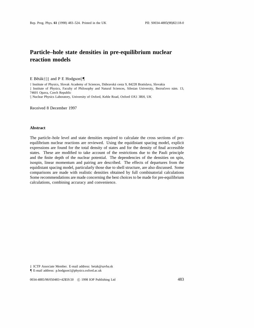
In the pre-equilibrium theories of nuclear reactions it is assumed that the excitationprocess takes place by successive nucleon–nucleon interactions in a series of stages. Eachinteraction produces a particle–hole (p–h) pair and each particle and hole is called anexciton. The first few states are therefore 2p1h, 3p2h, and so on. The number of excitonsn = p+h and the stages are labelled bys, so thatn = 2s+1. Usually each nucleon–nucleoninteraction produces another exciton, but occasionally a particle receives enough energy forit to be emitted; these are the pre-equilibrium reactions. The energy distribution of thesepre-equilibrium particles changes as the reaction proceeds; as expected, those emitted in theearlier stages have, on average, more energy than those emitted in later stages, as shown infigure 1 for 14.6 MeV neutrons on93Nb.
In general, the cross section for pre-equilibrium emission falls rapidly as the incidentenergy is shared among the nucleons of the target nucleus, and emission becomesincreasingly unlikely. Eventually the compound nucleus attains statistical equilibrium andemits particles very slowly until this is no longer energetically possible. These times are ona nuclear scale: the pre-equilibrium stage takes place in a time of the order of the transittime, about 10−22–10−20 s depending on the incident energy and target nucleus, whereasthe compound-nucleus stage takes about 10−18–10−16 s.
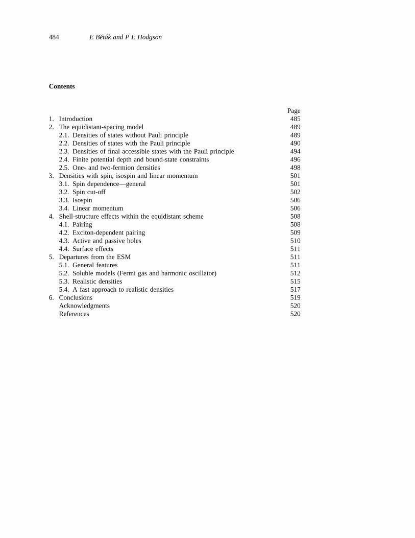
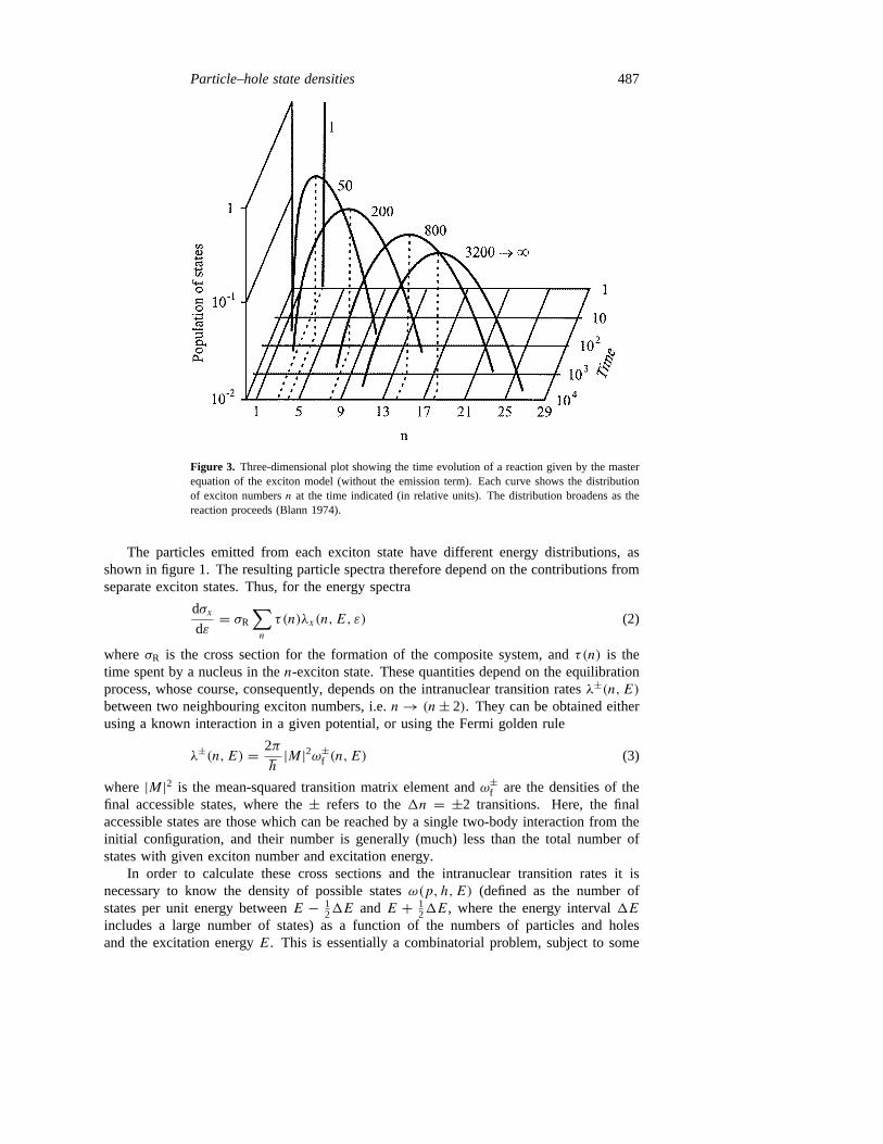
The number of excitons during the compound-nucleus stage fluctuates about a meanvalue, and although the probability of emission per unit time is extremely small, the totalcompound-nucleus cross section is often greater than the pre-equilibrium cross section.This is shown in figure 2 for the interaction of 14 MeV neutrons by titanium. For smallexciton numbers the cross section decreases, and then passes through a minimum at aboutn = 5, which marks the transition from pre-equilibrium to compound-nucleus emission.At higher energies, the switch from pre-equilibrium to the equilibrium emission occursat correspondingly higher exciton numbers. The broad peak at higher exciton numberscorresponds to compound-nucleus emission. A time-dependent picture of the developmentof a nuclear reaction with respect to the exciton numbers participating is shown in figure 3.
486 E Betak and P E Hodgson
Figure 1. The calculated spectra of nucleons emittedfrom the first, second and seventh stage of the93Nb(n, n′) reaction at 14.6 MeV. These are shownas the broken, dotted and chain curves, respectively.The total cross section (which includes the compoundnucleus cross section that dominates at small energies)is shown by the full curve (Hermanet al 1992).
Figure 2. The neutron emission cross section as afunction of exciton number for 14 MeV neutrons onTi (Chatterjee and Gupta 1981).
The rate of emissionλx(n,E, ε) of a nucleonx of energyε from a state ofn = p + hexcitons in a nucleus of excitation energyE, neglecting spin variables (apart from thestatistical weight factor(2sx + 1)) (see, e.g. Gadioli and Hodgson 1992, pp 19 and 235) isgiven by the product of a statistical weight factor, the cross sectionσ ∗INV (ε) of the inversereaction and the ratio of two state density functionsω(p, h,E)
λx(n,E, ε) = 2sx + 1
π2h3 µxεσ∗INV (ε)
ω(p − 1, h, U)
ω(p, h,E)(1)
whereµx is the nucleon reduced mass andU = E − Bx − ε is the energy of the residualnucleus which is produced in an(n− 1)-exciton state. Some authors include an additionalfactor which takes account of the charge composition of the excitons with respect to theejectile (see below). A similar equation can be obtained for cluster emission; this dependson the assumptions made about the complex particle creation and emission.
Particle–hole state densities 487
Figure 3. Three-dimensional plot showing the time evolution of a reaction given by the masterequation of the exciton model (without the emission term). Each curve shows the distributionof exciton numbersn at the time indicated (in relative units). The distribution broadens as thereaction proceeds (Blann 1974).
The particles emitted from each exciton state have different energy distributions, asshown in figure 1. The resulting particle spectra therefore depend on the contributions fromseparate exciton states. Thus, for the energy spectra
dσxdε= σR
∑n
τ (n)λx(n,E, ε) (2)
whereσR is the cross section for the formation of the composite system, andτ(n) is thetime spent by a nucleus in then-exciton state. These quantities depend on the equilibrationprocess, whose course, consequently, depends on the intranuclear transition ratesλ±(n,E)between two neighbouring exciton numbers, i.e.n→ (n± 2). They can be obtained eitherusing a known interaction in a given potential, or using the Fermi golden rule
λ±(n,E) = 2π
h|M|2ω±f (n,E) (3)
where|M|2 is the mean-squared transition matrix element andω±f are the densities of thefinal accessible states, where the± refers to the1n = ±2 transitions. Here, the finalaccessible states are those which can be reached by a single two-body interaction from theinitial configuration, and their number is generally (much) less than the total number ofstates with given exciton number and excitation energy.
In order to calculate these cross sections and the intranuclear transition rates it isnecessary to know the density of possible statesω(p, h,E) (defined as the number ofstates per unit energy betweenE − 1
21E andE + 121E, where the energy interval1E
includes a large number of states) as a function of the numbers of particles and holesand the excitation energyE. This is essentially a combinatorial problem, subject to some
488 E Betak and P E Hodgson
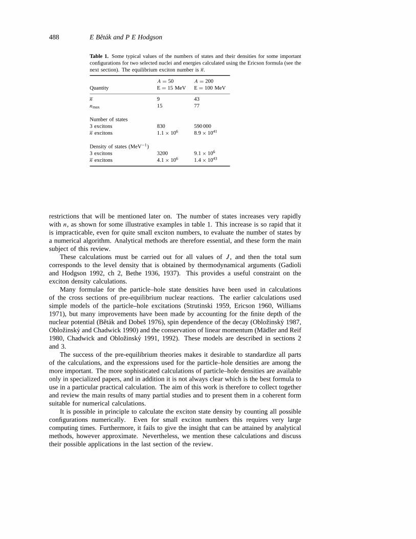
Table 1. Some typical values of the numbers of states and their densities for some importantconfigurations for two selected nuclei and energies calculated using the Ericson formula (see thenext section). The equilibrium exciton number isn.
A = 50 A = 200Quantity E= 15 MeV E= 100 MeV
n 9 43nmax 15 77
Number of states3 excitons 830 590 000n excitons 1.1× 10⁶ 8.9× 1041
Density of states (MeV−1)3 excitons 3200 9.1× 10⁶
n excitons 4.1× 10⁶ 1.4× 1043
restrictions that will be mentioned later on. The number of states increases very rapidlywith n, as shown for some illustrative examples in table 1. This increase is so rapid that itis impracticable, even for quite small exciton numbers, to evaluate the number of states bya numerical algorithm. Analytical methods are therefore essential, and these form the mainsubject of this review.
These calculations must be carried out for all values ofJ , and then the total sumcorresponds to the level density that is obtained by thermodynamical arguments (Gadioliand Hodgson 1992, ch 2, Bethe 1936, 1937). This provides a useful constraint on theexciton density calculations.
Many formulae for the particle–hole state densities have been used in calculationsof the cross sections of pre-equilibrium nuclear reactions. The earlier calculations usedsimple models of the particle–hole excitations (Strutinski 1959, Ericson 1960, Williams1971), but many improvements have been made by accounting for the finite depth of thenuclear potential (Betak and Dobes 1976), spin dependence of the decay (Oblozinsky 1987,Oblozinsky and Chadwick 1990) and the conservation of linear momentum (Madler and Reif1980, Chadwick and Oblozinsky 1991, 1992). These models are described in sections 2and 3.
The success of the pre-equilibrium theories makes it desirable to standardize all partsof the calculations, and the expressions used for the particle–hole densities are among themore important. The more sophisticated calculations of particle–hole densities are availableonly in specialized papers, and in addition it is not always clear which is the best formula touse in a particular practical calculation. The aim of this work is therefore to collect togetherand review the main results of many partial studies and to present them in a coherent formsuitable for numerical calculations.
It is possible in principle to calculate the exciton state density by counting all possibleconfigurations numerically. Even for small exciton numbers this requires very largecomputing times. Furthermore, it fails to give the insight that can be attained by analyticalmethods, however approximate. Nevertheless, we mention these calculations and discusstheir possible applications in the last section of the review.
Particle–hole state densities 489
2. The equidistant-spacing model
As a first approximation, we consider the equidistant-spacing model (ESM) suggested byBethe (1936). In this model all the single-particle levels are equally spaced in energy.In the ground state of a nucleus with mass numberA, all the A lowest-lying levels areoccupied and the highest one specifies the Fermi level. The excitation energy of a nucleusis distributed in some way among the excited particles above and the empty holes belowthe Fermi level. The ESM is a great simplification, but nevertheless it is very useful andgives quite a good energy dependence of the total density of states and at the same timeshows the basic properties of the densities and how and where they originate. The principaladvantages of the ESM is that it facilitates the analytical calculation of the exciton statedensities. If a more realistic spacings are used, this becomes practically impossible. Thefollowing sections give expressions for the state densities subject to various restrictions.
2.1. Densities of states without Pauli principle
Strutinski (1959) and Ericson (1960) showed that the ESM gives
ω(n,E) = ω(p, h,E) = gnEn−1
p!h!(n− 1)!(4)
wherep (h) is the number of particles (holes),n = p+ h is the total exciton number. Ifgis the single-particle level density,
ω(1, 0, Ep) = ω(0, 1, Eh) = g. (5)
The formula (4) can then be obtained by successive application of the recursion relations(see Gadioliet al 1973)
ω(p, 0, Ep) = 1
p
∫ Ep
0gω(p − 1, 0, U)dU
ω(0, h, Eh) = 1
h
∫ Eh
0gω(0, h− 1, U)dU
(6)
and finally
ω(p, h,E) =∫ E
0ω(p, 0, U)ω(0, h, E − U) dU. (7)
The last equation specifies the generally valid procedure used to obtain particle–holedensities from those for particles and for holes separately. The particle and hole densitiesin (7) need not necessarily be obtained from the ESM†.
To have some feeling for typical values of the densities of particle–hole states in real pre-equilibrium problems, we use also some knowledge beyond the scope of this review, namelythe range of energies and nuclei where the standard formulations of the pre-equilibriummodels are well justified. These arguments have been given by Agassiet al (1975), whoshowed that the necessary conditions for the statistical assumptions to be valid are
TP,n � (Tcoll,n, Tdec,n)� TNN (8)
whereTP,n is the Poincare recurrence time (the time needed for the statistical system toreturn to its original, very nonequilibrium configuration) for then-exciton configuration,Tcoll,n the average time interval between two successive interactions,Tdec,n the time of the
† An updated version of this approach appeared in a recent paper by Bogilaet al (1996a).
490 E Betak and P E Hodgson
decay of givenn-exciton state by emission of either particle or gamma andTNN the durationof the nucleon–nucleon interaction. If we express the conditions (8) in terms of energies,nuclei and their single-particle densities, we find that they are satisfied for nuclei withA & 40 andE & 15 MeV. The upper energy limit is given by the possible appearanceof non-nucleonic degrees of freedom, which limits the simple approach to about 150 MeVexcitation energy.
Table 1 gives the numerical values (rounded) for the most probable (or ‘equilibrium’)exciton numbern†, the maximum exciton numbernmax allowed by the Pauli principle andthe corresponding numbers of states and densities for the 3-exciton state (the most importantone for the nucleon emission under usual conditions) and the equilibrium exciton numbern, which dominates the equilibrium (compound nucleus) emission. The number of states atnmax is very small again, much less than at 3 excitons, and small departures from this tinyvalue can be fully attributed just to the approximate nature of the formulae. Table 1 showsthe numbers of states for nuclei and energies close to the lowest and highest ‘corners’ ofthe applicability of the model.
The total density of states which has to be compared with classical compound nucleus(i.e. equilibrium) theories is
ω(E) =∑n
1n=2
ω(n,E) (9)
where the summation is over all possible exciton states. The exciton number changes insteps of two becausen = 2s + 1 (see the introduction). The maximum exciton number islimited in practice by the Pauli principle (since two identical excitons cannot share the samestate) and, in the extreme case of very high energies, by twice the total number of nucleonsin a nucleus. (We do not discuss the applicability of the model at such energies here.)
The density of final accessible states needed for the calculation of intranuclear transitionrates (Williams 1970), corrected for the indistinguishability of excitons of the same type byRibansky et al (1973) is given by
ω−f = 12gph(n− 2)
ω+f = g(gE)2
2(n+ 1)
(10)
where the superscripts+ and− refer to the1n = ±2 transitions, respectively.
2.2. Densities of states with the Pauli principle
The inclusion of the Pauli principle greatly complicates the calculation of the density ofstates. In the languague of pre-equilibrium models, the Pauli principle requires that no twoexcitons of the same type are allowed to be in the same state, which implies that they cannothave the same energy.
The state densities have been obtained under these conditions by Bohning (1970). Hestudied the partition of an integerM into no morethanN integer parts. This problem wasessentially solved by Euler (1753). Let the energies of particle levels be 1/g, 2/g, 3/g, . . .and let there beN particles with total excitation energyE. The minimal energy needed dueto the Pauli principle isN(N + 1)/(2g), so that the ‘energy space’ available for excitationis
M = gE − 12N(N + 1). (11)
† We have used a more refined expression for state densities than that given by Ericson to obtainn, namely thatgiven in the next paragraph.
Particle–hole state densities 491
The number of partitionspN(M) of N particles with energyM satisfies the recurrencerelation (Williams 1971)
pN(M) = pN−1(M)+ pN(M −N) (12)
with
pN(0) = 1
p0(M) = δ0M. (13)
ForN > M, pN(M) is independent ofN and so is degenerate.The total number of particle–hole statesr(p, h,E) is obtained by folding those of the
particles and holes, as in (7)
r(p, h,E) =M∑m=0
pp(m)ph(M −m). (14)
The structure of (12) suggests that the resulting number of states and therefore also thedensities forM � N (as is the real case for nuclear reactions) can be approximated bya polynomial inM of order (N − 1). Neither (12) nor (14) are continuously increasingfunctions of energy, and they can remain constant even if the energyM is increased byseveral integer units.
While the recipe for obtaining the state densities within the ESM as given by Bohningis correct and precise, it is seldom used; simple analytical formulae or the relatively preciserealistic densities that are easily obtained with modern computers are generally preferred.
A feasible method to obtain an analytical formula was suggested by Williams (1971).Though the results are only approximate, it is quite accurate and it is easily programmedfor numerical calculation. The derivation is based on the Darwin–Fowler method fornonlocalized particles (see Munster 1969) with subsequent use of the Cauchy theorem inconjunction with the saddle-point approximation.
Let a1, a2, . . . be the occupation numbers of the single-particle states andε1, ε2, . . . thecorresponding energies. Then,∑
t
at = f∑t
at εt = Ef(15)
wheref stands for a given type of exciton (i.e. particles or holes).In the following, let us consider the ESM of for the particle and hole energies, which
are 1/g, 2/g, 3/g, . . . for particles and and 0, 1/g, 2/g, . . . for holes. The system partitionfunction is
Zsys= ZpZh (16)
whereZp andZh are the partition functions for particles and holes, respectively. They aresubject to the conditions (15), soZp for particles is given by the coefficient ofxf yEf inthe expansion of the function
Zp =∞∏i=1
(1+ xyi/g) (17)
and similarly for holes (Munster 1969, p 108, Williams 1971)
Zh =∞∏k=0
(1+ xyk/g). (18)
492 E Betak and P E Hodgson
These generating functions may be rewritten in the form
Zp = 1+∞∑m=1
xmy12m(m+1)/g∏m
i=1(1− yi/g)(19)
and similarly for holes. The number of states for particles and holes (see (14)) is
r(f, E) = 1
(2π i)2
∮ ∮Zf
dx dy
xf+1yE+1. (20)
Here,E is the energy of the system off fermions, wheref stands for eitherp or h.The integrals may be evaluated by the saddle-point method, and the resulting density is
ω(p, h,E) = gp+h(E − Aph)p+h−1
p!h!(p + h− 1)!2(E − αph) (21)
where2 is the Heaviside (step) function and
αph = 1
2g[(p2+ p)+ (h2− h)] (22)
is the minimal energy needed to putp particles andh holes in the levels, taking into accountthe Pauli principle and the correction term which lowers the energy in (21), and
Aph = 1
4g[(p2+ p)+ (h2− 3h)]. (23)
This term arises partially from the minimal energyαph and partially as the result of theintegration over the saddle in the complex plane when evaluating equation (20)†.
In the more general case of different spacingsg andg for particles and holes, the densityof n-exciton states becomes (Dobes and Betak 1976)
ω(p, h,E) = gpgh(E − Aph)p+h−1
p!h!(p + h− 1)!2(E − αph) (24)
where
αph = 1
2g(p2+ p)+ 1
2g(h2− h) (25)
and
Aph = 1
4g(p2+ p)+ 1
4g(h2− 3h). (26)
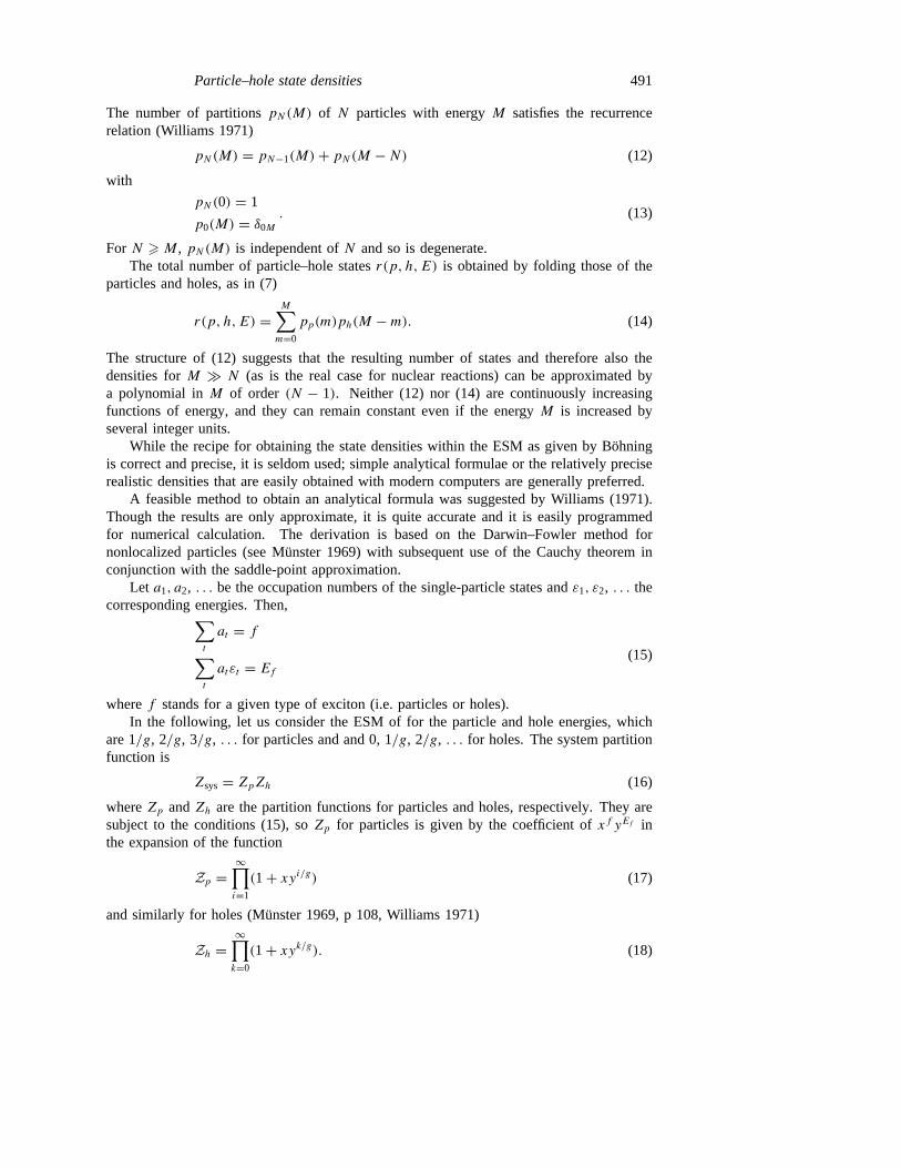
As in the preceding section, we make some comparisons in table 2 for two ‘casestudies’, with densities calculated using the Williams formula (21). The densities for lowexciton numbers remain practically at their previous values, whereas in the vicinity of theequilibrium exciton numbern the difference is essential (and is still much greater at higherexciton numbers) due to the rapidly growing correction term for the Pauli principleAph.
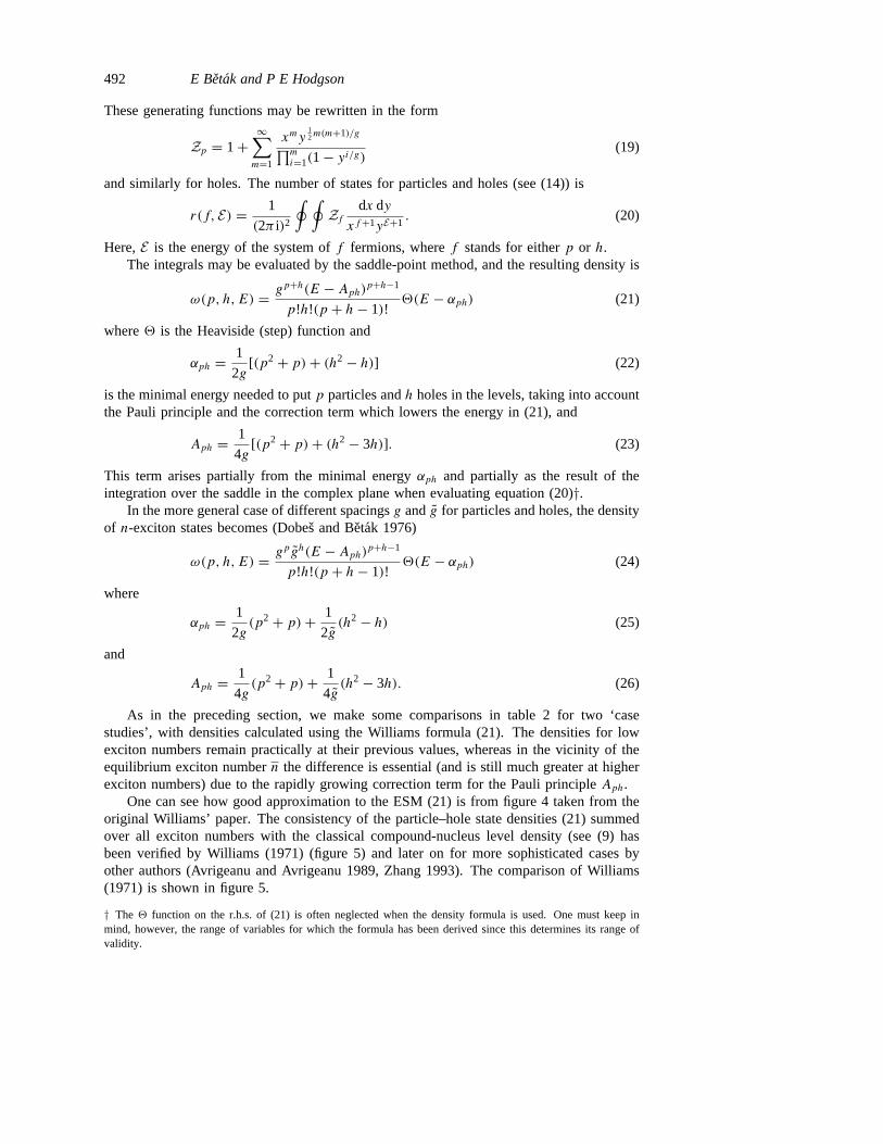
One can see how good approximation to the ESM (21) is from figure 4 taken from theoriginal Williams’ paper. The consistency of the particle–hole state densities (21) summedover all exciton numbers with the classical compound-nucleus level density (see (9) hasbeen verified by Williams (1971) (figure 5) and later on for more sophisticated cases byother authors (Avrigeanu and Avrigeanu 1989, Zhang 1993). The comparison of Williams(1971) is shown in figure 5.
† The2 function on the r.h.s. of (21) is often neglected when the density formula is used. One must keep inmind, however, the range of variables for which the formula has been derived since this determines its range ofvalidity.
Particle–hole state densities 493
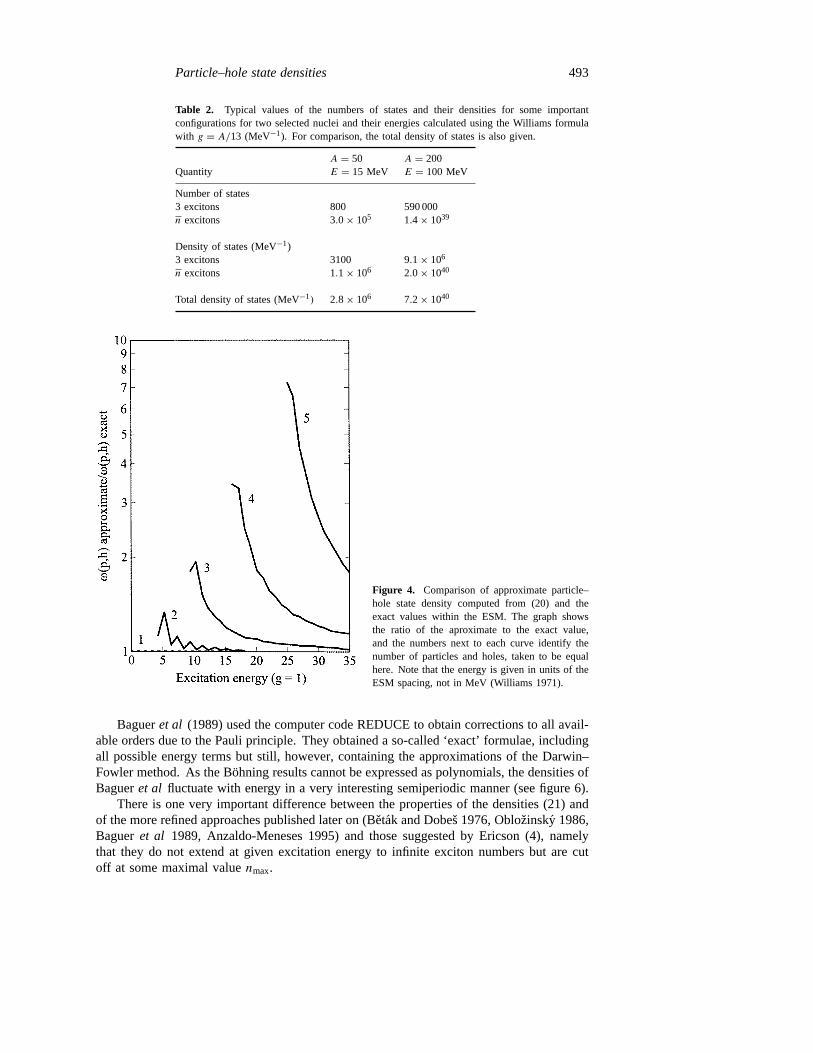
Table 2. Typical values of the numbers of states and their densities for some importantconfigurations for two selected nuclei and their energies calculated using the Williams formulawith g = A/13 (MeV−1). For comparison, the total density of states is also given.
A = 50 A = 200Quantity E = 15 MeV E = 100 MeV
Number of states3 excitons 800 590 000n excitons 3.0× 10⁵ 1.4× 1039
Density of states (MeV−1)3 excitons 3100 9.1× 10⁶
n excitons 1.1× 10⁶ 2.0× 1040
Total density of states (MeV−1) 2.8× 10⁶ 7.2× 1040
Figure 4. Comparison of approximate particle–hole state density computed from (20) and theexact values within the ESM. The graph showsthe ratio of the aproximate to the exact value,and the numbers next to each curve identify thenumber of particles and holes, taken to be equalhere. Note that the energy is given in units of theESM spacing, not in MeV (Williams 1971).
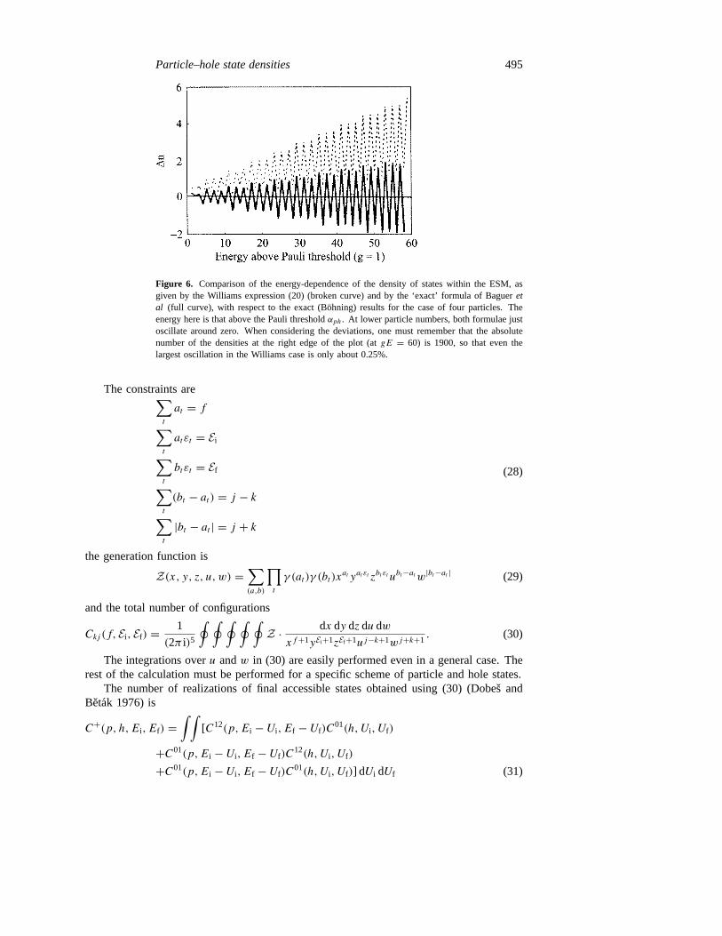
Bagueret al (1989) used the computer code REDUCE to obtain corrections to all avail-able orders due to the Pauli principle. They obtained a so-called ‘exact’ formulae, includingall possible energy terms but still, however, containing the approximations of the Darwin–Fowler method. As the Bohning results cannot be expressed as polynomials, the densities ofBagueret al fluctuate with energy in a very interesting semiperiodic manner (see figure 6).
There is one very important difference between the properties of the densities (21) andof the more refined approaches published later on (Betak and Dobes 1976, Oblozinsky 1986,Bagueret al 1989, Anzaldo-Meneses 1995) and those suggested by Ericson (4), namelythat they do not extend at given excitation energy to infinite exciton numbers but are cutoff at some maximal valuenmax.
494 E Betak and P E Hodgson
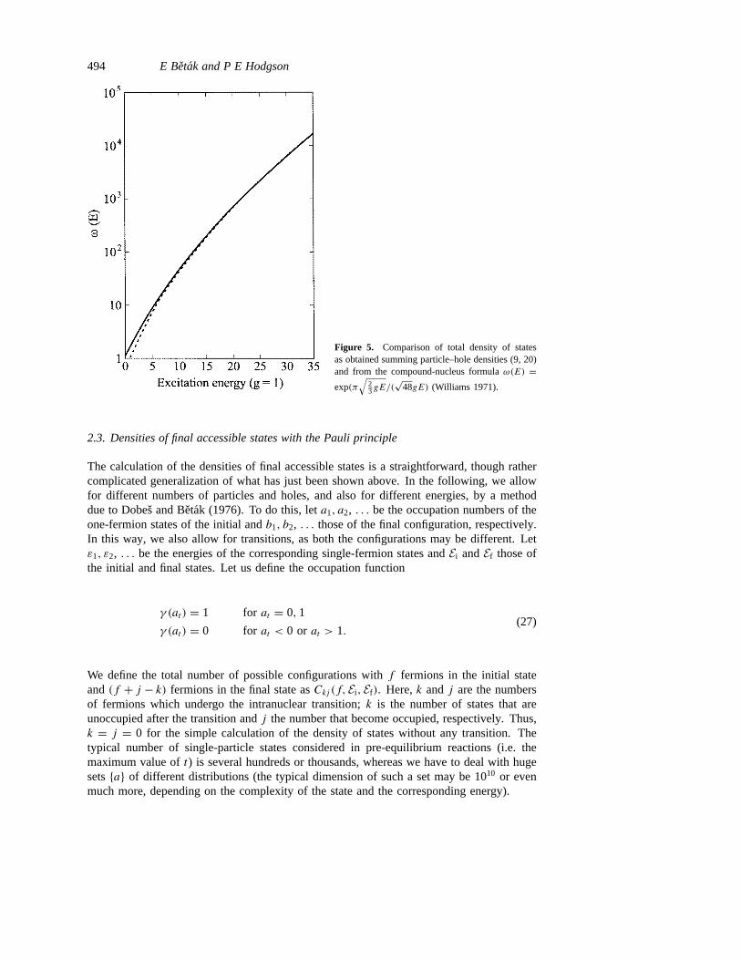
Figure 5. Comparison of total density of statesas obtained summing particle–hole densities (9, 20)and from the compound-nucleus formulaω(E) =exp(π
√23gE/(
√48gE) (Williams 1971).
2.3. Densities of final accessible states with the Pauli principle
The calculation of the densities of final accessible states is a straightforward, though rathercomplicated generalization of what has just been shown above. In the following, we allowfor different numbers of particles and holes, and also for different energies, by a methoddue to Dobes and Betak (1976). To do this, leta1, a2, . . . be the occupation numbers of theone-fermion states of the initial andb1, b2, . . . those of the final configuration, respectively.In this way, we also allow for transitions, as both the configurations may be different. Letε1, ε2, . . . be the energies of the corresponding single-fermion states andEi andEf those ofthe initial and final states. Let us define the occupation function
γ (at ) = 1 for at = 0, 1
γ (at ) = 0 for at < 0 or at > 1.(27)
We define the total number of possible configurations withf fermions in the initial stateand(f + j − k) fermions in the final state asCkj (f, Ei, Ef). Here,k andj are the numbersof fermions which undergo the intranuclear transition;k is the number of states that areunoccupied after the transition andj the number that become occupied, respectively. Thus,k = j = 0 for the simple calculation of the density of states without any transition. Thetypical number of single-particle states considered in pre-equilibrium reactions (i.e. themaximum value oft) is several hundreds or thousands, whereas we have to deal with hugesets{a} of different distributions (the typical dimension of such a set may be 1010 or evenmuch more, depending on the complexity of the state and the corresponding energy).
Particle–hole state densities 495
Figure 6. Comparison of the energy-dependence of the density of states within the ESM, asgiven by the Williams expression (20) (broken curve) and by the ‘exact’ formula of Bagueretal (full curve), with respect to the exact (Bohning) results for the case of four particles. Theenergy here is that above the Pauli thresholdαph. At lower particle numbers, both formulae justoscillate around zero. When considering the deviations, one must remember that the absolutenumber of the densities at the right edge of the plot (atgE = 60) is 1900, so that even thelargest oscillation in the Williams case is only about 0.25%.
The constraints are∑t
at = f∑t
at εt = Ei∑t
bt εt = Ef∑t
(bt − at ) = j − k∑t
|bt − at | = j + k
(28)
the generation function is
Z(x, y, z, u,w) =∑(a,b)
∏t
γ (at )γ (bt )xat yat εt zbt εt ubt−atw|bt−at | (29)
and the total number of configurations
Ckj (f, Ei, Ef) = 1
(2π i)5
∮ ∮ ∮ ∮ ∮Z · dx dy dz du dw
xf+1yEi+1zEf+1uj−k+1wj+k+1. (30)
The integrations overu andw in (30) are easily performed even in a general case. Therest of the calculation must be performed for a specific scheme of particle and hole states.
The number of realizations of final accessible states obtained using (30) (Dobes andBetak 1976) is
C+(p, h,Ei, Ef) =∫ ∫
[C12(p,Ei − Ui, Ef − Uf)C01(h, Ui, Uf)
+C01(p,Ei − Ui, Ef − Uf)C12(h, Ui, Uf)
+C01(p,Ei − Ui, Ef − Uf)C01(h, Ui, Uf)] dUi dUf (31)
496 E Betak and P E Hodgson
and similarly for the other possible processes.The densities of final accessible states on the energy shellEi = Ef = E are
ω+f (p, h,E) = C+(p, h,E,E)/ω(p, h,E)ω0
f (p, h,E) = C0(p, h,E,E)/ω(p, h,E)
ω−f (p, h,E) = C+(p − 1, h− 1, E,E)/ω(p, h,E).
(32)
The equations (31) and (32) are valid in general. For simplicity, we useg = 1 in thefollowing formulae. The explicit results for the densities of final accessible states whenonly the highest power of energy is retained, are (Dobes and Betak 1976)
ω−f (p, h,E) ≈1
2ph(n− 2)
[1− n− 1
8(n− 2)(E − Aph)((p − 1)(p − 2)+ (h− 1)(h− 2))
]ω0
f (p, h,E) ≈E − Aph
2n
(p(p − 1)
[1− n(p + 2)
2(E − Aph)]
+p(p − 1)
[1− n(h+ 2)
2(E − Aph)]+ 4ph
[1− n(n− 1)
4(E − Aph)])
ω+f (p, h,E) ≈(E − Aph)2
2(n+ 1)
[1− n+ 1
n(E − Aph)(
5
8p(p − 1)+ 5
8h(h− 1)+ ph+ 1
2n
)].
(33)
The expression forω−f is identical to that obtained by Oblozinsky et al (1974) by a muchsimpler and sufficiently transparent method where, unfortunately, the same form of the Pauliprinciple correction is assumed for different exciton states.
More complete expressions than that given by (33) (up to the second order of corrections)for the densities of final accessible states were obtained by Isaev (1985). However, eventhe (33) are not often used and they are replaced by simpler, though less precise results.
For practical use, an even more straightfoward approximation is available. If we ingorethe influence of the Pauli principle on the1n = −2 intranuclear transitions where it is leastimportant, the steady-state equilibrium conditions give directly (Ribansky et al 1973)†
ω+f (p, h,E) =g
2(n+ 1)
[g(E − Ap+1,h+1)]n+1
[g(E − Aph)]n−1(34)
in close analogy with (10).
2.4. Finite potential depth and bound-state constraints
The importance of the finiteness of the nuclear potential well on pre-equilibrium decay wasfirst pointed out by Blann (1972). He gave the correction for the two exciton configurations,which mostly influence the calculation of the pre-equilibrium nucleon emission, namely2p1h and 1p1h. Under simplifying assumptions such as the neglect of the Pauli principle,expressions can be obtained easily by the integration procedure already given in (6).
The correct derivation of the densities of states taking the Pauli principle into accountshould, however, be made using the methods of statistical physics that give (20). The holegeneration function including the finiteness of the nuclear potential well is not that givenby (18), but (Betak and Dobes 1976)
Zh =gEF−1∏k=0
(1+ xyk/g) (35)
† The first densities of final states with some correction due to the Pauli principle have been published by Cline(1972b). The form of the Pauli principle correction is not given there correctly.
Particle–hole state densities 497
whereEF is the Fermi energy. This leads to
Zh = 1+∞∑n=1
xny12n(n−1)/g
n∏k=1
1− yEF−(n−k)g
(1− yk/g) . (36)
Hence, one straightforwardly finds
ω(p, h,E) = gpghh∑l=0
∑j
Clj
h (−)l2(E − αph − lEF+ g(lh− j))
× (E − Aph − lEF+ g(lh− j))n−1
p!h!(p + h− 1)!(37)
with
C00h = 1
Clj
h =∑
0<k1<···<kl<hk1+k2+···+kl=j
1 for lh− 12l(l − 1) 6 j 6 1
2l(l + 1)
Clj
h = 0 for j < 12l(l + 1) and forj > lh− 1
2l(l − 1).
(38)
Using ∑j
Clj
h =(h
l
)(39)
and neglecting the factorsg(lh − j) in the energy terms on the r.h.s. of (37) we finallyarrive at the easily usable formula
ω(p, h,E) = gpghh∑l=0
(h
l
)(−)l2(E − αph − lEF)
(E − Aph − lEF)n−1
p!h!(p + h− 1)!. (40)
For approximate calculations, the above equation can be further reduced to
ω(p, h,E) ≈ gp+hh∑l=0
(h
l
)(−)l2(E − lEF)
(E − lEF)n−1
p!h!(p + h− 1)!. (41)
The associated transition rates can be derived in the same manner as the precedingsection for the case of an infinite well (Betak and Dobes 1976). The final formulae arerather lengthy and not very suitable for practical use. For such cases, they can be replacedby
ω±f (p, h,E;EF) ≈ ω±f (p, h,E;EF = ∞) ω(p ± 1, h± 1, E;EF)
ω(p ± 1, h± 1, E;EF = ∞) (42)
whereω±f (p, h,E;EF = ∞) are the rates for the infinite well, given, for example, by (32).For a sufficiently wide range of energies, this expression agrees within 5% with the exactone (Betak and Dobes 1976).
Distinguishing between bound and unbound states in the theory of pre-equilibrium decay(Feshbach 1973), corresponding to the multistep compound and multistep direct reactions,led to an increased demand for explicit expressions for state densities for bound states, foruse in multistep compound theories (Feshbachet al 1980, Tamuraet al 1982, Nishiokaetal 1986, 1988a and 1989).
Though these densities are only a special case of (37) or (40), with the same type ofenergy constraint as we had for holes (holes are not allowed to have higher energy than theFermi energy,EF) to be applied also to particles (their energy must not exceed now the
498 E Betak and P E Hodgson
particle binding energyB), they have not been used immediately. Stankiewiczet al (1985)derived the densities with the help of integral equations of the type given by (6) and (7)neglecting the Pauli principle. Kalbach (1981) consistently distinguished active and passiveparticles and holes and finally Oblozinsky (1986) gave an analogue to (40). His expressionreads
ω(p, h,E) = gpghp∑k=0
h∑l=0
(p
k
)(h
l
)(−)l2(E − αph − kB − lEF)
× (E − Aph − kB − lEF)n−1
p!h!(p + h− 1)!(43)
or, approximately
ω(p, h,E) ≈ gp+hp∑k=0
h∑l=0
(p
k
)(h
l
)(−)l2(E − kB − lEF)
(E − kB − lEF)n−1
p!h!(p + h− 1)!. (44)
Similar equations have been reported by some other groups (Zhang and Yang 1988, Maoand Guo 1993).
2.5. One- and two-fermion densities
So far, we have divided the excitons into particles and holes. The real nucleus, however,is not composed of nucleons of just one type, but of neutrons and protons. We should,therefore, make a further distinction in our calculations. The formulae given above areusually refered to as one-fermion ones to distinguish them from the two-fermion case,where we consider the neutrons separately from the protons†.
A straightforwad way to do this has already been introduced in the derivation of densitiesby Williams (1971). Let us denote the proton particles (holes) asπ (π ) and the neutronones asν (ν). The total number of excitonsn is as it was in the one-fermion case,n = π + π + ν + ν. The two-component density is now
ω(π, π, ν, ν, E) = gππ g ππ gν
ν g νν
(E − Bππνν)n−1
π !π !ν!ν!(n− 1)!(45)
with
Bππνν = 1
4gπ(π2+ π)+ 1
4gπ(π2− 3π)+ 1
4gν(ν2+ ν)+ 1
4gν(ν2− 3ν). (46)
The two-fermion densities with shell corrections were published by Berger and Martinot(1974). Their calculation stems from the same background as that of Williams (1971)and Dobes and Betak (1976), but it avoids the use of the Cauchy residue theorem. Atmodest energies (up to about 80 MeV), the results agree well with those of Williams, butat significantly higher energies and high exciton numbers, Williams formula seems to bean overestimation. The method of Berger and Martinot is also used to study shell effects,which are found to be significant in some cases.
The complete two-fermion calculations can be found in a paper by Gupta (1981), whoused the two-fermion master equations to describe equilibration in the case in which neutronsand protons are distinguished. The two-fermion version of the exciton model was studiedin detail by Dobes and Betak (1983). They finalized the form of the transition rates for all
† Rather frequently, one meets the terms ‘one-component’ and ‘two-component’. These are unfortunately notused consistently in all papers, as some denote the two-fermion case as ‘four-component’ and consequently theone-fermion one as ‘two-component’.
Particle–hole state densities 499
occuring transitions (in the two-fermion case, there are more different transitions than only1n = ±2, as in the one-fermion formulations) and investigated the different matrix elementsgoverning the intranuclear transitions. Subsequent important refinements can be found inKalbach (1986) and Hermanet al (1989), but these papers are essentially concerned withother aspects of the densities and will be treated in detail in other sections of this review.
One can treat some selected problems of the two-fermion approach (see Betaket al 1974,Betak and Dobes 1979, Avrigeanuet al 1997), or make calculations taking full account ofthe two-fermion nature of the problem (Gupta 1981, Dobes and Betak 1983, Kalbach 1984,1986, Jingshang 1994, Fu 1994)†. These calculations are very time-consuming and theagreement with the data is of the same quality as in the one-fermion formulation with theinclusion of some effective charge factor. In these two-fermion calculations, however, onehas to fix the relative strength of different types of intranuclear transitions and there isvery little information from the experimental data which could usefully distinguish amongvarious suggested approaches.
In practice, therefore, another method is used, namely the introduction of some effectivecharge factor in the emission rates (different charge factors were proposed by various authors,see below)‡. This method is only an effective and approximate one, and must be understoodas such. Strictly speaking, the appearance of the effective charge factor in the emissionrates is an intrusive element in the pre-equilibrium calculations, as it violates the properequilibrium limit, some physicists therefore deny its presence in the emission rates.
The philosophy behind the charge factor is probably best justified in the case of thefactor K introduced by the Milano group (Braga-Marcazzanet al (1972) for the lowestemitting state, Birattariet al (1973), and finally Gadioli-Erba and Sona (1973), see alsoGadioli and Hodgson (1992, section 2.5.4)). Let us for simplicity consider the case of a(p, n) reaction. The incoming proton may interact with either a proton or a neutron, thuscreating a 3-exciton configuration of type 2ππ or πνν. Neutron emission is impossiblefrom the first possible 3-exciton configuration and leads to a 2-exciton configuration of aπν type in the residual nucleus from the latter one. The ratio of densities on the r.h.s. of(1) in this case is therefore
ω(1, 0, 0, 1, U)
ω(2, 1, 0, 0, E)+ ω(1, 0, 1, 1, E)(47)
in reality, whereas in the one-fermion formulation of the pre-equilibrium decay one has
ω(2, 1, U)
ω(2, 1, E). (48)
Therefore, if we use the simpler one-fermion formulation, we have to multiply the emissionrate in this case by the ratioK of both the expressions (47) and (48). This ratio may beeasily evaluated assuminggπ = gπ = gν = gν = g/2 and neglecting the Pauli principlecorrection. This procedure yieldsKν(3) ≈ 0.667.
It is easy to prove that (see Gadioli and Hodgson 1992, section 2.5.4, p 87)
Kπ +Kν = 2 (49)
for every exciton number, independently of the incident projectile. In the very same way,one can also derive the charge factorK for the cluster (e.g.α) emission.
† We do not consider here two-fermion calculations which go beyond the ESM model, as they will be treated insection 5.‡ Similarly, the charge factors are also used in other models, for example in the hybrid model (Blann 1973, 1975).Their connection to the particle–hole state densities is not emphasized and we shall not discuss them here.
500 E Betak and P E Hodgson
The charge factorK of the Milano group clearly assumes that (i) intranucleartransitions to more complex states are governed only by the available phase space, i.e.the matrix element of a transition〈|M|2〉 is independent of the initial proton/neutron excitoncomposition and is the same for an excitation of a proton as for a neutron; (ii) the never-come-back approximation may be used for its derivation, i.e. there is no configurationmixing and/or feeding from more complex states eventually reached earlier in the reaction,and—the most serious assumption—(iii) we are fully justified to replace the single-fermionstate density in the denominator of (48) by the sum of all two-fermion configurations (of thesame exciton number) entering the denominator of (47), i.e. we have the right to effectivelyconsider the exciton configurations which do not contribute to the emission at all in thespecific case. In addition, there are (iv) some simplifying assumptions (neglecting the Pauliprinciple and assuming allg’s are equal) that enable the charge factorK to be expressed in aconvenient closed form. All the above assumptions, however, may be subject to discussionand none of them is of a basic importance. From a physical point of view we consider theK factor to be the clearest and best justified of all charge factors developed.
Another charge factorR was suggested by Cline (1972a). Its philosophy is differentfrom that of theK factor. To illustrate, we shall consider the same reaction as above,namely(p, n). If we assume that the interaction between the neutron and the proton is ofthe same strength, the incoming proton excites another proton with probabilityZ/A, and aneutron with probabilityN/A. In the 3-exciton state, we have two particles (and one hole).It follows that of these two particles there are 1+ Z/A protons andN/A neutrons, onaverage. As we have two particles, the probability of obtaining a neutron isN/(2A), andthis is a factor which should be multiplied by the one-fermion emission rates to account forproper charge composition. For states significantly different from the initial configurationand close to equilibrium we assume that the charge composition of excitons, which is thesame (proportional to) as that of the composite system, which givesN/A for the neutronandZ/A for the proton emission. Obviously,
Rπ +Rν = 1 (50)
at each stage of the reaction. The philosophy of theR factor can be easily put into closedformulae for both nucleon and cluster emission, and we refer the reader to the originalsource in this case (Cline 1972a).
The equilibrium limit ofR for nucleon emission in the case ofZ = N is clearly 12 (and
e.g. 38 for the α-particles). This implies a disagreement with the equilibrium emission
expression by the same factor introduced artificially from outside and is therefore notjustified. This handicap is of a much deeper nature than the objections raised againsttheK factor above.
To remove the improper equilibrium limit of theR factor, Kalbach (1977) introducedanother charge factorQ. It has a proper compound-nucleus limit of 1, and the explicitexpression is
Qβ(p) =(A
Z
)πβ (AN
)νβ πβ !νβ !
pβ !Rβ(p) (51)
whereR is the charge factor introduced earlier,pβ is the mass number of the emittedparticle consisting ofπβ protons andνβ neutrons. As is easily seen, the ratio of the protonto the neutron emission is amplified by a factor ofN/Z with respect to that obtained usingtheR charge factor for the lowest exciton state contributing to the nucleon emission. Thegeneral behaviour of theQ factor is similar to that of theK factor of the Milano group. Ittends to the value of 1 at equilibrium, but there is no normalization condition of type (49)which should be valid throughout the reaction.
Particle–hole state densities 501
A closely related factorQ has been obtained from comparison of the one- and two-fermion results by Gupta (1981). His factor forZ = N coincides with that of Kalbach, butdiffers in the other cases†.
When using the one-fermion formulation with some form of the charge factor, we mustbe aware of the introduced shortcomings. Apart from that, the numerical results are nearlyindistinguishable, up to a necessary renormalization of the transition matrix element〈|M|2〉by a factor of two in the case of theR factor with respect to the three others‡.
The proper approach would be a real two-fermion calculation, but this is very seldomperfomed, and we find only the one-fermion calculations in practice. Because of thedisadvantages of all the charge factors proposed until now, and especially for the purityof the model approach and to keep the well-established equilibrium limit, many calculationsare performed (except in the one-fermion version of the model) without any effective chargefactor.
3. Densities with spin, isospin and linear momentum
3.1. Spin dependence—general
In the compound nucleus (i.e. equilibrium) case, the nucleon emission rates are (Gadioliand Hodgson 1992, p 256)
λπ,ν([E, J ]ε→ [U, S]) = 1
h
ρ(U, S)
ρ(E, J )
S+ 12∑
j=|S− 12 |
J+j∑l=|J−j |
Tlj (ε) (52)
where the emission proceeds from a composite system of excitation energyE and spinJto the residual nucleus of an energyU and spinS, and l is the orbital momentum of theemitted particle. The densities are assumed to be factorized (see, e.g. Kikuchi and Kawai(1968, section 1.7, p 32), Bohr and Mottelson (1969, p 155 and appendix 2B), Gadioli andHodgson (1992, section 2.1, p. 40))
ρ(E, J ) = ω(E) 2J + 1
2√
2πσ 3exp
(− (J +
12)
2
2σ 2
). (53)
whereσ is the spin cut-off parameter of the compound nucleus.Similarly, in the pre-equilibrium case one has (Shiet al 1987)
λπ,ν([E, J, n]ε→ [U, S, n− 1]) = 1
h
ρ(n− 1, U, S)
ρ(n,E, J )Rπ,ν(n)
S+ 12∑
j=|S− 12 |
J+j∑l=|J−j |
Tlj (ε). (54)
The particle–hole state densityρ(n,E, J ) is
ρ(n,E, J ) = g(gE − Aph)n−1
p!h!(n− 1)!Rn(J ) (55)
† One more charge factor has been suggested by Zhang (1990, 1993), yielding in practice close results to the twoQ factors given above.‡ The effective replacement of the two-fermion densities by the one-fermion ones also includes the assumptionof the relative interaction ofππ , πν, andνν pairs. Thus Gadioliet al (1971) and Gupta (1981) assume equalstrength of all these interactions, Cline (1972a) and Kalbach (1977) excitations proportional toN/A andZ/A,Blann et al (Blann and Mignerey 1972, Blann 1973) proportional toσπν/σνν , Dobes and Betak (1983) use thesame assumption and approximate it by a value of 3 and recently Kalbach (1995c) assumes the strength of theππ
andνν interaction to be by a factor of 1.7 higher than that of theπν one. In her former paper (Kalbach 1986),she relates the absolute values of the matrix elements in the one- and the two-fermion case, the former one beingroughly one half of the latter.
502 E Betak and P E Hodgson
whereg is the single-particle level density, andAph is the correction term due to the Pauliprinciple. In the limiting case of an infinite number of levels, the spin distribution is
Rn(J ) = 2J + 1
2√
2πσn3exp
(− (J +
12)
2
2σn2
)(56)
whereσn is the spin cut-off parameter. This form is in practice assumed and also used forfinite numbers of levels. This distribution is normalized such that∑
J
(2J + 1)Rn(J ) ≈ 1 (57)
so that although it contains the factorσ 3n , the main effect of increasingσ 3
n is to broaden thedistribution rather than to decrease the overall magnitude.
We need to distinguish between the cut-off parameter for a fully equilibrated compoundnucleus and that appropriate for the pre-equilibrium stage.
The densities of particle–hole states with spin are the basis for pre-equilibrium angular-momentum dependent calculations. For the transition rates, one usually assumes that theyare factorized. For the1n = −2 transitions, the densities of the final accessible states are(Oblozinsky 1987, Oblozinsky and Chadwick 1990)
ω+f (n,E, J ) = ω+f (n,E)X↓nJ (58)
with the energy partω+f (n,E) equal to the spin-independent density of the final accessiblestates for such a transition (e.g. (10) or (34), and the spin part is (Oblozinsky 1987)
XnJ↓ = 1
Rn(J )
∑j4Q
R1(Q)F (Q)Rn−1(j4)1(Qj4J ). (59)
The density of the inverse process is obtained via the steady-state equilibrium conditions.In (59), theR’s are the spin parts of the density of states,J is the spin of the state (itis conserved during the transition) and is decomposed into the spin of the inert ‘core’,j4
andQ, the spin of the exciton initiating given transition (j1 to j3 are spins of the excitonscreated in such a transition). The proper relation of all spins is expressed by1(Qj4J ),which is 1 for |Q− j4| 6 J 6 Q+ j4 and 0 otherwise and by functions
F (Q) =∑j3j5
(2j5+ 1)R1(j5)(2j3+ 1)F (j3)
(j5 j3 Q12 0 − 1
2
)2
(60)
and the angular momentum density of pair states
F(j3) =∑j1j2
(2j1+ 1)R1(j1)(2j2+ 1)R1(j2)
(j1 j2 j312 − 1
2 0
)2
. (61)
An approximation to these formulae has been given by Bogilaet al (1995b), which alsofacilitates this kind of calculations with smaller computers.
3.2. Spin cut-off
The first expression for the spin-dependent particle–hole density was given in the originalwork of Williams (1971). Generally, the spin cut-off parameter is a product of the meannumber of unpaired particles and holesνph and an averaged square of the projection of theindividual spins on the axis〈m2〉 (Ericson 1960)
σ 2 = νph〈m2〉. (62)
Particle–hole state densities 503
According to Ericson (1960), the number of unpaired particles and holes increases withtemperaturet in the compound-nucleus theory,
νph = gt. (63)
Williams (1971) took the same relation as a starting point to express the spin cut-off inthe particle–hole scheme. As the temperature at a given excitation energyE can be easilyexpressed via the exciton number using the state density
t =[
d lnω(p, h,E)
dE
]−1
(64)
we straightforwardly obtain
σ 2n =
gE − 18n
2
n− 1〈m2〉. (65)
The form of (65) assumes equal numbers of particles and holes. From (65) the limitingvalue ofσ 2
n for small n, the most significant one for the pre-equilibrium emission, is
gE
n− 1〈m2〉 (66)
which is clearly wrong forn = 1 and also implies that the lower the number of particlesand holes, the higher the number of unpaired particles and holes—an obvious contradiction.For these reasons the Williams formula for the spin-dependent density has never been usedin real calculations.
Combining (62) and (63) from the classical theory of the compound nucleus we obtainthe spin cut-off in the form
σ 2 = 〈m2〉gt = g〈m2〉√E − E0
a(67)
whereE0 is the pairing correction (see below). The spin projection is〈m2〉 ∝ A2/3 with theproportionality contant varying from 0.146 (Jensen and Luttingen 1952) to 0.24 (Facchiniand Saetta-Menichella 1968).
The difficulties of the Williams suggestion (65) were overcome by Ignatyuk and Sokolov.They (Sokolov 1972, Ignatyuk 1973, Ignatyuk and Sokolov 1973, 1978, Ignatyuk 1983)derived the spin-dependent density from the general expression for the statistical sum forthe particles. In the small-momentum approximation (projection of total momentum ofnucleusM � 〈m〉(p + h)) they obtained for the spin cut-off factor
σ 2n = 〈m2〉 (p + h)
2
p + h− 1≈ 〈m2〉(p + h). (68)
The case of Fermi particles (which is the real situation) is more complicated. Using thesaddle-point method (and again for the case of small momenta), the spin cut-off parametertakes the form
σ 2n =
2g
β〈m2〉(1+ e−γ ) (69)
whereβ and γ are determined by a set of coupled equations (see the original papers fordetails). The cut-offσ 2
n determined in this way is an increasing function of energy, at leastfor smalln. In some models (e.g. for the Fermi gas), it reaches its maximumσ 2
n ≈ σ 2 closeto n = n (Ignatyuk and Sokolov 1978) and decreases thereafter. For a global understanding
504 E Betak and P E Hodgson
of pre-equilibrium phenomena, however, the differences between different models are notso essential, so we concentrate our attention on then < n (or evenn� n) region†.
As an approximation to the method of Ignatyuk and Sokolov (1973), Fu (1986) solvedthese equations. Introducing a critical temperatureTc (= 210/3.5, where10 is the ground-state pairing gap (see below)) and the corresponding most probable exciton number at thistemperature,nc, and spin cut-off,σ 2
c = gTc〈m2〉, he obtained
σ 2n = σ 2
c ln 4
(n
nc
)(E − Ethr
E
)x(70)
with x being a polynomial of the second order in√n/nc, andEthr is the threshold energy
needed for the realization of a given state (see Fu 1984). In the case of no pairing andequidistant levels, it coincides with the quantityαph (equation (22)) in the Williams formula.
However, even these expressions are often considered to be inconvenient for practicaluse and a dependence of the type (72) is preferred.
According to Feshbachet al (1980), a relation similar to (70) also holds in the case ofstates with specified exciton number; the resulting exciton spin cut-off is proportional to theexciton number,
σ 2n = ct
n
n. (71)
If we neglect the linear term in the relation between the temperature and excitation energyand take it simply in the formE = at2, the exciton-dependent spin cut-off can be expressedas
σ 2n = 0.16nA2/3. (72)
A similar relation has been reported by Reffo and Herman (1982), Plyuiko (1978), andGardner and Gardner (1989). The proportionality constants, when referred to explicitly,were 0.28 (Reffo and Herman) and 0.16 (Plyuiko). The original method of Reffo andHerman (1982) based on the BCS calculations, has been tailored to low exciton numbers,whereas the formula of Feshbachet al (1980), on the other hand, is more appropriate atn ≈ n.
In their subsequent papers, Herman and Reffo (1987b, 1992) used their combinatorialcode to obtain so-called realistic level densities (see section 5.3). From the fit to the levelsproduced by their computer code, the energy dependence of the spin cut-off is weak. Theyfound that the energy-averaged spin cut-off can be approximated by
σ 2n = cnA2/3+ 0.1A2/3+ 4 (73)
with c = 0.22. This is approximately
σ 2n = cnA2/3 (74)
with c ≈ 0.26. If we want to keep at least some energy dependence, we can write
c = 0.24+ 0.0038E. (75)
However,σ 2n for 2-exciton configurations of type 2p0h (1π1ν) are about 5 units higher
than those for the 1p1h (1π1π or 1ν1ν) ones; this effect reduces to 2 units for 4-excitonconfigurations and is negligible for 6 excitons and more. Withc given by (75),
σ 2n = n(0.24+ 0.0038E)A2/3. (76)
† The formalism of Ignatyuk and Sokolov can be applied also straightforwardly to the two-fermion case (e.g. Fu1992).
Particle–hole state densities 505
Herman and Reffo (1992) also studied the effects of the shell structure. Generally, theWilliams formula is found to be good, though at lower energies some differences may besignificant. However, collective phenomena such as deformation are clearly absent in theWilliams formula.
The detailed study of spin effects by Chadwick and Oblozinsky (1992) used
σ 2n = n
(2mεav
3
)(77)
which in the case of the equidistant scheme gives
εav = 2p(p + 1)
ng
ρ(p + 1, h, E)
ρ(p, h, E)− gn+ EF (78)
where
E = E − (p − h)EF. (79)
Finally, one obtains
σ 2n = n0.282A2/3 (80)
very close to the results of Herman and Reffo.Bogila et al (1992) studied both the exciton dependence of the spin cuf-off as well as
the influence of the Pauli principle. The formula (69) identifies〈m2〉 with σ 2s , the value for
the single-particle states. The energy dependence ofσ 2s is found to be (from rather general
considerations)
σ 2s (ε) = σ 2
s (EF)ε/EF (81)
which implies for particles
σ 2p (ε) = 〈m2〉(p + E/EF) (82)
and
σ 2h (ε) = 〈m2〉(h− E/EF) (83)
for holes.The effect of the Pauli principle is to decrease the number of exciton degrees of freedom,
which becomes
n∗ = n(1− αph/E) (84)
and therefore
σ 2n = n∗〈m2〉 = n(1− αph/E)〈m2〉 = n(1− n2/n2
max)〈m2〉 (85)
wherenmax is the maximum exciton number allowed at a given energy due to the Pauliprinciple†.
† Anzaldo-Meneses (1997) gives a procedure for level density (based on the grand partition function) for an‘arbitrary periodic spectrum’. It is also suitable to obtain the spin distributions (in the case of harmonic oscillatoror similar ‘periodic’ solution), but the particles are considered asbosonsand therefore no equivalent of the Pauliprinciple correction is introduced.
506 E Betak and P E Hodgson
3.3. Isospin
In nuclear reactions, states with different values of isospin can be populated. The lowestlying states have the lowest possible isospin (equal to itsz-component). At some higherexcitation energy, a set of states with one additional unit of isospin, theT> states, willbegin. The densities of both sets of states,T< and T>, increase exponentially with theexcitation energy, but since theT> states begin at higher energy, they will always be farless numerous than theT< states.
The implications of this for pre-equilibrium decay have been studied by Kalbach(Kalbach-Clineet al 1974, Kalbach 1993, 1995b, c). In proton- and3He-induced reactionson targets with isospinT0, a fraction of 1/(2T0 + 1) of the composite nucleus formationcross section forms states with the isospinT = T>, whereas the remaining (usually major)fraction of the cross section, namely 2T0/(2T0 + 1) goes to the more abundantT< states.In neutron- andα-particle induced reactions, only states of the ground-state isospin arepopulated.
The influence of these considerations on the particle emission depends on the extent ofthe isospin conservation in nuclear reactions. If the isospin is mixed completely, the decaywill be essentially that of the very much more abundantT< states. This implies that theproton and the neutron emission proceed essentially in the same manner. On the other hand,if isospin is conserved, there is a chance to see theT>-state decay. For theT> states, theneutron emission is hindered because the residual states of the lowest isospin are forbidden.This implies a significant relative enhancement of the proton emission.
To calculate isospin effects in nuclear reactions it is therefore necessary to determinehow much the isospin is conserved or mixed, and what is the isospin symmetry energy.The evaluation of the particle–hole densities, accouning for isospin, assumes that there isone-to-one correspondence between states of the same isospinT in isobaric nuclei,
ω(p, h,E, T , Tz = T ) = ω(p, h,E + Esym(T , T − 1), T , T − 1)
= ω(p, h,E + Esym(T , T − 2), T , T − 2) = · · · (86)
whereEsym is the symmetry energy, i.e. the excitation energy of the lowest state (of anyexciton number) of isospinT in the nucleus considered. The semi-empirical mass formulayields here in a simple case of volume plus surface symmetry energy (see Kalbach 1995c)
Esym(T , Tz) = (110A−1− 133A−4/3)(T 2− Tz2) [MeV] . (87)
If we write the analogue of (24) with isospin included (omitting now all other details, suchas pairing and the influence of the irregularities in the level scheme due to the shell structureetc), the corresponding particle–hole density is
ω(p, h,E, T ) = gn(E − Aph)n−1
p!h!(n− 1)!fT (p, h, T ) (88)
where the Pauli correction term is now (Kalbach 1995b)
AphT ≈ Aph + Esym(T , Tz). (89)
The functionfT in (88) is the correction factor for states with good isospin, which is takenfrom Kalbach (1993). If isospin is asumed to be completely mixed, the symmetry energyEsym is zero and the correction factorfT is unity.
3.4. Linear momentum
Madler et al (1978) suggested the use of linear momentum to describe the angulardistributions. The angular distributions arise from a multiplicative factor in the emission
Particle–hole state densities 507
rates, i.e. the basic expression for the emission is the same as before, but with an additionalangle-dependent factor (normalized to 1 after integration over angle). In practice, theyuse an average value for the single-particle linear momentum, which is derived using verysimple assumptions for a quantity dependent on the exciton number.
In their subsequent paper (Madler and Reif 1980), they switched to the total linearmomentum, calculated from the partition function (of statistical mechanics). A closedformula is given only for the limiting case of zero initial velocity, though the recipe is moregeneral. Finally the linear momentum is decomposed intop‖ andp⊥.
The last paper in their series (Madler and Reif 1982) uses the same basic idea, but witha more consistent statistical derivation. The momentum is kept as a single (vector) variablein the emission rates and not decomposed into two parts. The results of Madler and Reifhave been used in the cascade-exciton model suggested and used by Gudimaet al (1983).Unfortunately, their inclusion of linear momentum to obtain the angular distributions is notformulated sufficiently clearly, and the paper is usually not recognized as such.
Chadwick and Oblozinsky (1991, 1992) completed the work. Just as the usual particle–hole state densities can be derived by using recurrence relations starting from more simpleconfigurations (equations (5)–(7)), the densities with specified linear momentum can beobtained in a similar way. The final general expression (Oblozinsky and Chadwick 1990)is
ω(p, h,E,K) = 1
p!h!
∫i=1· · ·∫i=p
∫j=1
· · ·∫j=h
δ
(E −
p∑i=1
εi +h∑j=1
εj
)δ
(K −
p∑i=1
ki +h∑j=1
kj
)
×p∏i=1
ω1(ki)2(ki − kF) d3ki
h∏j=1
ω1(kj )2(kF− kj ) d3kj (90)
where the single-particle energiesε are counted for both particles and holes from the bottomof the potential well andki andkj are the single-particle and -hole momenta, respectively.The number of single-particle states with momenta in the range(k, k + dk)
dN(k)
dk= 4πk2ω1(k) (91)
is connected to the density of states in the energy spaceω1(ε) = dN(ε)/dε, which yieldsthe relation between the two densities
ω1(k) = ω1(ε)/(4πmk). (92)
From this we obtain
ω1(k) = A43πk
3F
(93)
for the Fermi-gas model and
ω1(k) = g
4πmk(94)
for the ESM.The evaluation of the particle–hole state densities with linear momentum is now
a relatively straightfoward, though extremely complicated and time-consuming process.Formally, we can write these densities as
ω(p, h,E,K) = ω(p, h,E)M(p, h,E,K). (95)
508 E Betak and P E Hodgson
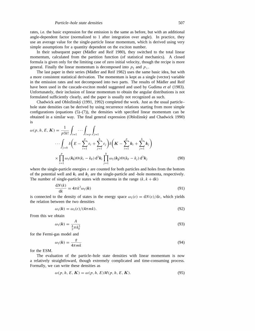
Figure 7. Comparison of the linear-momentum distribution(multipled by 4πK2) for exact and statistical Gaussiansolutions of state densities with linear momentum, for anexcitation energy of 5 MeV in a Fermi-gas nucleus. Theaccuracy of the Gaussian solution increrases rapidly withincreasingn (Chadwick and Oblozinsky 1992).
For large exciton number, one can apply statistics and the central limit theorem gives
M(p, h,E,K) = 1
(2π)3/2σ 3n
exp(−K2/2σ 2n ) (96)
whereσ 2n = n〈(kproj
i )2〉 is the width of the distribution. For exciton numbers, however,some departures from the form of (96) are observed. Fortunately, they are significant onlyfor the 1p1h configuration, where the real distribution is practically triangular. Everywhereelse the Gaussian form of (96) can be successfully used (see figure 7). This importantconclusion gives a practical and very useful recipe to calculate the angular distributions (fordetails, see Chadwick and Oblozinsky 1992). Recently, an approach to the level densitieswith linear momentum and the corresponding angular distributions has been successfullyreported for the Fermi-gas case (Blann and Chadwick 1998).
4. Shell-structure effects within the equidistant scheme
The assumption of equidistant levels is a rather useful concept, but it is neverthelessoversimplified when compared with the real situation. A significant improvement may beachieved if we introduce at least some features of real nuclei. Probably the most profoundof them is the influence of pairing and possibly also the existence of irregularities, such asthe energy gaps as a manifestation of closed shells and subshells, in the single-particle levelschemes.
4.1. Pairing
The formulae for the level density in the compound-nucleus case are sharply increasingfunctions of the excitation energy. However, due to the strong tendency of nucleons (of thesame kind) to couple in pairs, one has to add an additional energy to break such pairs fornuclei with an even number of nucleons of either type. Thus, this energy (in even-Z and/oreven-N nuclei) is effectively not available to increase the density of levels. Very roughly,
Particle–hole state densities 509
this pairing-energy correction is (see, e.g. Ignatyuk 1983)
E′ = E − E0pair (97)
whereE0pair is the conventional pairing energy correction, i.e. zero for odd–odd nuclei, and
a quantity close to 12A−1/2 MeV for odd-A nuclei and twice that value for the even–evenones (Mashnik 1993).
Nowadays calculations commonly use the values of both pairing energy corrections forthe neutrons and the protons together with the single-particle level density as a parameter.The first extensive detailed study of that type by Gilbert and Cameron (1965) is possiblystill the most extensive (with a large tables of values) and the most frequently used one.
A slight modification of the above approach is the back-shifted Fermi-gas model.Therein, the corrections may be both positive and negative, and they are (in general) nonzerofor all nuclei. Suitable sets of paremeters can be found in a paper by Dilget al (1973) ormore recently Iljinovet al (1992).
The simplest way to include the pairing correction in the particle–hole density is inexactly the same way as in the compound-nucleus case, i.e. to take the pairing-energycorrection (together with individual values for the single-particle level density) for eachindividual nucleus from the tables (Gilbert and Cameron 1965, Facchini and Saetta-Menichella 1968, Dilget al 1973, Rohr 1984, Capoteet al 1987, Iljinov et al 1992,Mengoni and Nakajima 1994) as the same values for all exciton numbers.
In fact, the first pre-equilibrium calculations were so rough that they reproduced onlythe main features of the emitted spectra and anything more detailed has been omitted. Soonafterwards, however, indications emerged that one should account for the statistics of thenuclei involved as well as details of the particle–hole level densities (Lee and Griffin 1972,Ignatyuk and Sokolov 1972, Grimeset al 1973a). Later, the use of (at least) pairing alsobecame necessary in these reactions.
As an improvement on the ESM in the vicinity of closed shells, a schematic modelof shell structure was proposed for the compound-nucleus case by Rosenzweig (1957). Tosimulate the bunching and degeneracy of nuclear states, Rosenzweig divided the equidistant-spacing sequence of states into groups separated by gaps. As the final effect, the pairingenergy is effectively modified by an amount which depends on the average degeneracy of thelevels in the neighbourhood of the Fermi level as well as on their average spacing therein.This idea was later applied to the pre-equilibrium decay by Cline (1971) and in a moreconsistent way by Betak (1975); the corresponding results showed the usefulness of suchan approach. However, inclusion of this effect requires not well-defined quantities such asthe average degeneracy and the average level density near the Fermi level. In practice, theRosenzweig effect is seldom considered in pre-equilibrium calculations.
4.2. Exciton-dependent pairing
A simple treatment of pairing corrections in the same way as in the compound-nucleustheory is useful, but for finer study one needs a more detailed approach (Ignatyuk andSokolov 1973, 1978). Let10 be the ground-state pairing gap and1(E, n) the excited-statepairing gap. The ground-state pairing gap10 is readily given, e.g. Dilget al (1973) use10 = 2
√117.6/(gA) MeV; the excited-state pairing gap1 is calculated from the pairing
theory (see, e.g. Moretto 1975) using10 and g. The exciton-number dependent pairingcorrection (which reduces the ‘available’ excitation energy as in (97)) is (Ignatyuk and

510 E Betak and P E Hodgson
Sokolov 1973)
Epair(U, n) = g
4[12
0−12(E, n)]. (98)
The pairing correctionE0pair for the total state density is equal toEpair evaluated along the
most probable exciton numbern for E > 3.15E0pair and is (Ignatyuk and Sokolov 1973,
1978, Fu 1986, 1992)
E0pair = Epair(E, n) = 1
4g120. (99)
For the two-fermion case of (45), the pairing corrections are sums over the neutronsand the protons, namely
Epair(E, nπ , nν) = Epair(Eπ, nπ)+ Epair(Eν, nν) (100)
formally the same as in the one-fermion case. With the exception of very low excitationenergies, the energyEπ can be expressed as
Eπ = nπE/n (101)
and similarly forEν . The neutron and proton parts of the spin cut-off take formally justthe same expressions as in the one-component case, only with the total quantities (excitonnumber, excitation energy) replaced by those related to the given type of nucleons.
4.3. Active and passive holes
There is a long-standing problem about the proper treatment of the number of particles andholes in excited nuclei in connection with their statistics. Obviously, an even–even targetnucleus is 0p0h in its ground state. Impacting nucleon can be considered on one hand asa 1p excitation, but on the other hand we may equally require that all nuclei havep = hthroughout all their development. The problem is of very little importance for nuclei inthe vicinity of closed shells (closed-shell nucleimustbe of p = h at all stages, i.e. 0p0hin their ground state) and for the case of both projectile and ejectile being nucleons. Butif we are far off these conditions (especially for reactions with clusters either on input oremitted), the whole problem emerges more profoundly.
It has been addressed already by Lee and Griffin (1972), and in a much more completestudy by Kalbach (1975), who introduced the shell-shifted equispacing model with activeand passive particles and/or holes. In pre-equilibrium calculations we are interested only inparticles (holes) which represent degrees of freedom; that is those which have permutableexcitation energy. ‘Passive’ particles (holes) which are fixed adjacent to the Fermi level arenot counted. However, they contribute to the Pauli energy. If the Fermi surface is takento be half-way between the last filled and first vacant single-particle states in the nucleonground-state configuration, then the ground state is always of the typep = h = 0 if wealso count the passive excitons, and correspondinglyp = h for every excited state (underthe same condition). Usually, the passive particles (holes) are not counted. For a compositesystem formed by nucleon bombardment, there is usually a passive hole at the Fermi level,so thatp > h. Thus, the usual starting configuration ofn = 1 can be classified as a 1p+ 1passive hole andn = 3 (2p1h) as a 2p + 1h+ 1 passive hole.
The original idea has been further developed by Kalbach (1987, 1989, 1995a, 1995b).If we keep just the leading term, the correction is (Kalbach 1987)
AKalb(p, h) = q2
g− p(p + 1)+ h(h+ 1)
4g(102)
whereq = max(p, h). A similar question has been raised by Zhang and Yang (1988), buttheir results are correct only forp = h.
Particle–hole state densities 511
4.4. Surface effects
The weakly bound nucleons from open shells near the Fermi level are the ones that areeasily excited. The finite-depth formula for the particle–hole density (41) makes it possibleto study such behaviour. Already Gmuca and Ribansky (1980) have used the effective depthof the nucleon potential well as a parameter and they obtained harder spectra of emittednucleons and therefore better agreement with the data.
The more attention we devote to the surface region, the more we need accurate leveldensities in that region. Kalbach (1985) introduced an additional correction near the Fermisurface. She started from the energy dependence of the Fermi-gas level densities,
gFG(ε) = kF√ε = g0
√ε/EF (103)
wherekF is the Fermi momentum (see (107) below). Obviously, the energyε is measuredfrom the bottom of the potential well, and not from the Fermi energy. If the averageparticle energy isεp (and similarly for holesεh), the average single-particle level density(for particles) is
g = g(εp) = g0
√EF+ εpEF
(104)
and the average single-hole level density
g = g(εh) = g0
√EF− εhEF
. (105)
In the case of an infinite potential well (or of excitation energyE less than the Fermi energyEF) we have
εp = εh = E/n (106)
and a more complicated estimate (due to corrections introduced in (37) or (40)) can beobtained for other potentials (Kalbach 1985, Chadwick and Oblozinsky 1992, Avrigeanuand Avrigeanu 1994, Blann and Chadwick 1998). These refinements improve the fit to thedata.
The role of surface effects has been revitalized by studies of the imaginary part of theoptical potential for pre-equilibrium processes (Sato and Yoshida 1994) and in a recent studyby Avrigeanuet al (1996).
5. Departures from the ESM
5.1. General features
All the considerations up to now have been made within the equidistant-spacing scheme,though in some cases with additional terms describing some facets of the behaviour ofrealistic nuclei. The ESM works suprisingly well, but it is nevertheless an oversimplification.
We get much closer to the real situation if we use some improved scheme of levels.A starting point may be the Fermi-gas or harmonic-oscillator model; more sophisticatedapproaches benefit from a realistic scheme of single-particle levels. In principle, the generalmethod of Dobes and Betak (1976) (see chapter 2.2) allows for an arbitrary level scheme,though only the ESM was considered originally. In some cases, the particle–hole statedensities and particle–hole densities of final accessible states can be obtained as closed-form expressions. More often, however, it is not feasible to perform analytically all the
512 E Betak and P E Hodgson
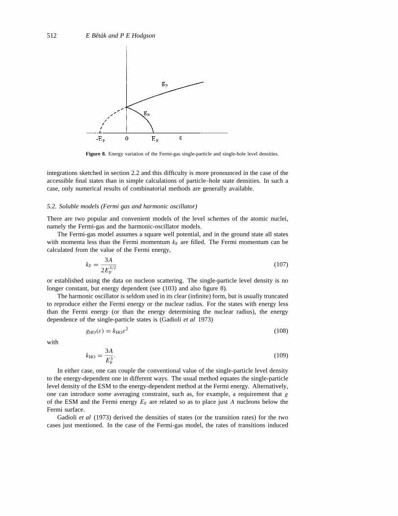
Figure 8. Energy variation of the Fermi-gas single-particle and single-hole level densities.
integrations sketched in section 2.2 and this difficulty is more pronounced in the case of theaccessible final states than in simple calculations of particle–hole state densities. In such acase, only numerical results of combinatorial methods are generally available.
5.2. Soluble models (Fermi gas and harmonic oscillator)
There are two popular and convenient models of the level schemes of the atomic nuclei,namely the Fermi-gas and the harmonic-oscillator models.
The Fermi-gas model assumes a square well potential, and in the ground state all stateswith momenta less than the Fermi momentumkF are filled. The Fermi momentum can becalculated from the value of the Fermi energy,
kF = 3A
2E3/2F
(107)
or established using the data on nucleon scattering. The single-particle level density is nolonger constant, but energy dependent (see (103) and also figure 8).
The harmonic oscillator is seldom used in its clear (infinite) form, but is usually truncatedto reproduce either the Fermi energy or the nuclear radius. For the states with energy lessthan the Fermi energy (or than the energy determining the nuclear radius), the energydependence of the single-particle states is (Gadioliet al 1973)
gHO(ε) = kHOε2 (108)
with
kHO = 3A
E3F
. (109)
In either case, one can couple the conventional value of the single-particle level densityto the energy-dependent one in different ways. The usual method equates the single-particlelevel density of the ESM to the energy-dependent method at the Fermi energy. Alternatively,one can introduce some averaging constraint, such as, for example, a requirement thatg
of the ESM and the Fermi energyEF are related so as to place justA nucleons below theFermi surface.
Gadioli et al (1973) derived the densities of states (or the transition rates) for the twocases just mentioned. In the case of the Fermi-gas model, the rates of transitions induced
Particle–hole state densities 513
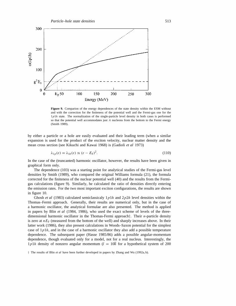
Figure 9. Comparion of the energy dependences of the state density within the ESM withoutand with the correction for the finiteness of the potential well and the Fermi-gas one for the1p1h state. The normalization of the single-particle level density in both cases is performedso that the potential well accommodates justA nucleons from the bottom to the Fermi energy(Smith 1989).
by either a particle or a hole are easily evaluated and their leading term (when a similarexpansion is used for the product of the exciton velocity, nuclear matter density and themean cross section (see Kikuchi and Kawai 1968) is (Gadioliet al 1973)
λ1p(ε) = λ1h(ε) ∝ (ε − EF)2. (110)
In the case of the (truncanted) harmonic oscillator, however, the results have been given ingraphical form only.
The dependence (103) was a starting point for analytical studies of the Fermi-gas leveldensities by Smith (1989), who compared the original Williams formula (21), the formulacorrected for the finiteness of the nuclear potential well (40) and the results from the Fermi-gas calculations (figure 9). Similarly, he calculated the ratio of densities directly enteringthe emission rates. For the two most important exciton configurations, the results are shownin figure 10.
Ghoshet al (1983) calculated semiclassicaly 1p1h and 2p2h level densities within theThomas–Fermi approach. Generally, their results are numerical only, but in the case ofa harmonic oscillator, the analytical formulae are also presented. The method is appliedin papers by Blinet al (1984, 1986), who used the exact scheme of levels of the three-dimensional harmonic oscillator in the Thomas-Fermi approach†. Their n-particle densityis zero atnEF (measured from the bottom of the well) and sharply increases above. In theirlatter work (1986), they also present calculations in Woods–Saxon potential for the simplestcase of 1p1h, and in the case of a harmonic oscillator they also add a possible temperaturedependence. The subsequent paper (Hasse 1985/86) adds a possible angular-momentumdependence, though evaluated only for a model, not for a real nucleus. Interestingly, the1p1h density of nonzero angular momentum (l = 10h for a hypothetical system of 200
† The results of Blinet al have been further developed in papers by Zhang and Wu (1992a, b).
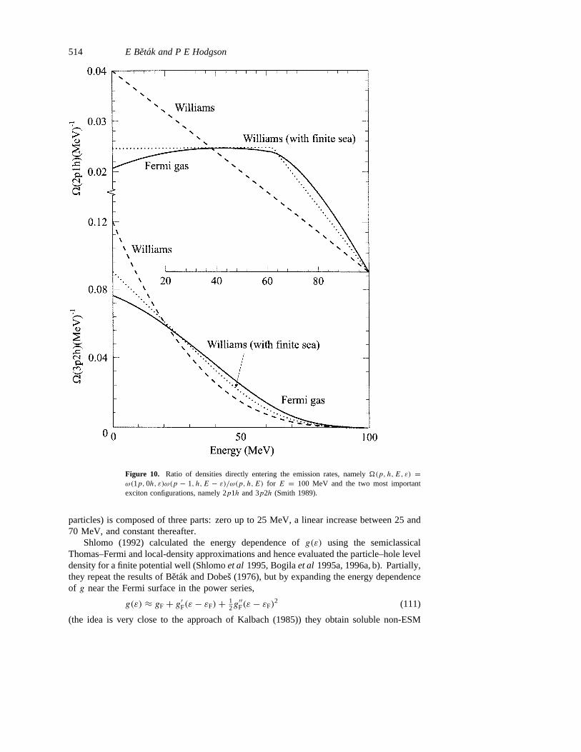
514 E Betak and P E Hodgson
Figure 10. Ratio of densities directly entering the emission rates, namely�(p, h,E, ε) =ω(1p, 0h, ε)ω(p − 1, h, E − ε)/ω(p, h,E) for E = 100 MeV and the two most importantexciton configurations, namely 2p1h and 3p2h (Smith 1989).
particles) is composed of three parts: zero up to 25 MeV, a linear increase between 25 and70 MeV, and constant thereafter.
Shlomo (1992) calculated the energy dependence ofg(ε) using the semiclassicalThomas–Fermi and local-density approximations and hence evaluated the particle–hole leveldensity for a finite potential well (Shlomoet al 1995, Bogilaet al 1995a, 1996a, b). Partially,they repeat the results of Betak and Dobes (1976), but by expanding the energy dependenceof g near the Fermi surface in the power series,
g(ε) ≈ gF+ g′F(ε − εF)+ 12g′′F(ε − εF)
2 (111)
(the idea is very close to the approach of Kalbach (1985)) they obtain soluble non-ESM
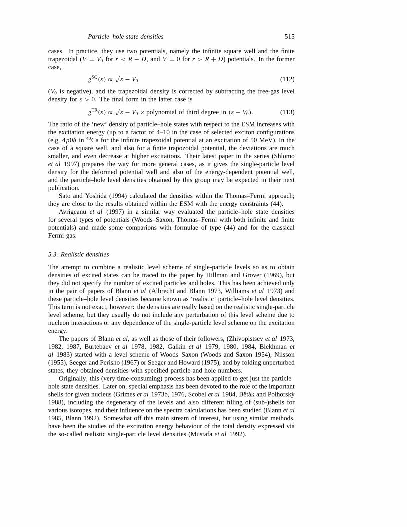
Particle–hole state densities 515
cases. In practice, they use two potentials, namely the infinite square well and the finitetrapezoidal (V = V0 for r < R −D, andV = 0 for r > R +D) potentials. In the formercase,
gSQ(ε) ∝√ε − V0 (112)
(V0 is negative), and the trapezoidal density is corrected by subtracting the free-gas leveldensity forε > 0. The final form in the latter case is
gTR(ε) ∝√ε − V0× polynomial of third degree in(ε − V0). (113)
The ratio of the ‘new’ density of particle–hole states with respect to the ESM increases withthe excitation energy (up to a factor of 4–10 in the case of selected exciton configurations(e.g. 4p0h in 40Ca for the infinite trapezoidal potential at an excitation of 50 MeV). In thecase of a square well, and also for a finite trapozoidal potential, the deviations are muchsmaller, and even decrease at higher excitations. Their latest paper in the series (Shlomoet al 1997) prepares the way for more general cases, as it gives the single-particle leveldensity for the deformed potential well and also of the energy-dependent potential well,and the particle–hole level densities obtained by this group may be expected in their nextpublication.
Sato and Yoshida (1994) calculated the densities within the Thomas–Fermi approach;they are close to the results obtained within the ESM with the energy constraints (44).
Avrigeanu et al (1997) in a similar way evaluated the particle–hole state densitiesfor several types of potentials (Woods–Saxon, Thomas–Fermi with both infinite and finitepotentials) and made some comparions with formulae of type (44) and for the classicalFermi gas.
5.3. Realistic densities
The attempt to combine a realistic level scheme of single-particle levels so as to obtaindensities of excited states can be traced to the paper by Hillman and Grover (1969), butthey did not specify the number of excited particles and holes. This has been achieved onlyin the pair of papers of Blannet al (Albrecht and Blann 1973, Williamset al 1973) andthese particle–hole level densities became known as ‘realistic’ particle–hole level densities.This term is not exact, however: the densities are really based on the realistic single-particlelevel scheme, but they usually do not include any perturbation of this level scheme due tonucleon interactions or any dependence of the single-particle level scheme on the excitationenergy.
The papers of Blannet al, as well as those of their followers, (Zhivopistsevet al 1973,1982, 1987, Burtebaevet al 1978, 1982, Galkinet al 1979, 1980, 1984, Blekhmanetal 1983) started with a level scheme of Woods–Saxon (Woods and Saxon 1954), Nilsson(1955), Seeger and Perisho (1967) or Seeger and Howard (1975), and by folding unperturbedstates, they obtained densities with specified particle and hole numbers.
Originally, this (very time-consuming) process has been applied to get just the particle–hole state densities. Later on, special emphasis has been devoted to the role of the importantshells for given nucleus (Grimeset al 1973b, 1976, Scobelet al 1984, Betak and Polhorsky1988), including the degeneracy of the levels and also different filling of (sub-)shells forvarious isotopes, and their influence on the spectra calculations has been studied (Blannet al1985, Blann 1992). Somewhat off this main stream of interest, but using similar methods,have been the studies of the excitation energy behaviour of the total density expressed viathe so-called realistic single-particle level densities (Mustafaet al 1992).
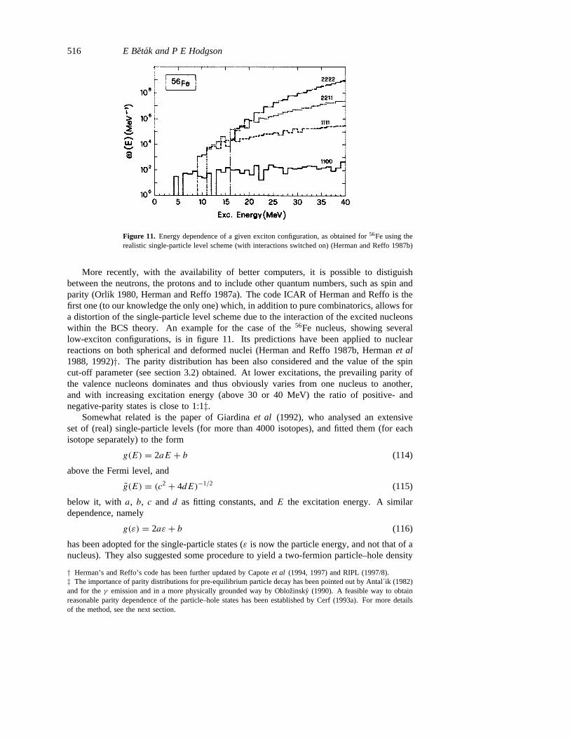
516 E Betak and P E Hodgson
Figure 11. Energy dependence of a given exciton configuration, as obtained for56Fe using therealistic single-particle level scheme (with interactions switched on) (Herman and Reffo 1987b)
More recently, with the availability of better computers, it is possible to distiguishbetween the neutrons, the protons and to include other quantum numbers, such as spin andparity (Orlik 1980, Herman and Reffo 1987a). The code ICAR of Herman and Reffo is thefirst one (to our knowledge the only one) which, in addition to pure combinatorics, allows fora distortion of the single-particle level scheme due to the interaction of the excited nucleonswithin the BCS theory. An example for the case of the56Fe nucleus, showing severallow-exciton configurations, is in figure 11. Its predictions have been applied to nuclearreactions on both spherical and deformed nuclei (Herman and Reffo 1987b, Hermanet al1988, 1992)†. The parity distribution has been also considered and the value of the spincut-off parameter (see section 3.2) obtained. At lower excitations, the prevailing parity ofthe valence nucleons dominates and thus obviously varies from one nucleus to another,and with increasing excitation energy (above 30 or 40 MeV) the ratio of positive- andnegative-parity states is close to 1:1‡.
Somewhat related is the paper of Giardinaet al (1992), who analysed an extensiveset of (real) single-particle levels (for more than 4000 isotopes), and fitted them (for eachisotope separately) to the form
g(E) = 2aE + b (114)
above the Fermi level, and
g(E) = (c2+ 4dE)−1/2 (115)
below it, with a, b, c and d as fitting constants, andE the excitation energy. A similardependence, namely
g(ε) = 2aε + b (116)
has been adopted for the single-particle states (ε is now the particle energy, and not that of anucleus). They also suggested some procedure to yield a two-fermion particle–hole density
† Herman’s and Reffo’s code has been further updated by Capoteet al (1994, 1997) and RIPL (1997/8).‡ The importance of parity distributions for pre-equilibrium particle decay has been pointed out by Antal´ik (1982)and for theγ emission and in a more physically grounded way by Oblozinsky (1990). A feasible way to obtainreasonable parity dependence of the particle–hole states has been established by Cerf (1993a). For more detailsof the method, see the next section.
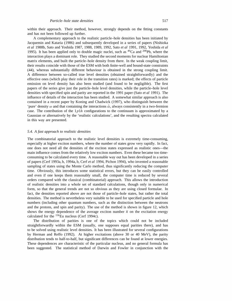
Particle–hole state densities 517
within their approach. Their method, however, strongly depends on the fitting constantsand has not been followed up further.
A complementary approach to the realistic particle–hole densities has been initiated byJacquemin and Kataria (1986) and subsequently developed in a series of papers (Nishiokaet al 1988b, Sato and Yoshida 1987, 1988, 1989, 1992, Satoet al 1991, 1992, Yoshidaet al1995). It has been applied only to double magic nuclei, such as40Ca and208Pb, where theinteraction plays a dominant role. They studied the second moments for nuclear Hamiltonianmatrix elements, and built the particle–hole density from there. In the weak coupling limit,their results coincide with those of the ESM with both finite-well and bound-state constraints(44), whereas substantially different behaviour is obtained in the strong coupling limit.A difference between so-called true level densities (obtained straightforwardly) and theeffective ones (which play their role in the transition rates) is marked; the effects of particleemission on level density has also been studied (and found to be negligible). The firstpapers of the series give just the particle–hole level densities, while the particle–hole leveldensities with specified spin and parity are reported in the 1991 paper (Satoet al 1991). Theinfluence of details of the interaction has been studied. A somewhat similar approach is alsocontained in a recent paper by Koning and Chadwick (1997), who distinguish between the‘pure’ densityω and that containing the interactionsω, always consistently in a two-fermioncase. The contribution of the 1p1h configurations to the continuum is approximated by aGaussian or alternatively by the ‘realistic calculations’, and the resulting spectra calculatedin this way are presented.
5.4. A fast approach to realistic densities
The combinatorial approach to the realistic level densities is extremely time-consuming,especially at higher exciton numbers, where the number of states grow very rapidly. In fact,one does not need all the densities of the exciton states expressed as realistic ones—themain influence comes from the relatively low exciton numbers. Even these became too time-consuming to be calculated every time. A reasonable way out has been developed in a seriesof papers (Cerf 1993a, b, 1994a, b, Cerfet al 1994, Pichon 1994), who invented a reasonablesampling of states using the Monte Carlo method, thus significantly reducing the computertime. Obviously, this introduces some statistical errors, but they can be easily controlledand even if one keeps them reasonably small, the computer time is reduced by severalorders compared with the classical (combinatorial) approach. This allows the introductionof realistic densities into a whole set of standard calculations, though only in numericalform, so that the general trends are not so obvious as they are using closed formulae. Infact, the densities reported above are not those of particle–hole states, but rather the totaldensities. The method is nevertheless very suitable to be used for specified particle and holenumbers (including other quantum numbers, such as the distinction between the neutronsand the protons, and spin and parity). The use of the method is shown in figure 12, whichshows the energy dependence of the average exciton numbern on the excitation energycalculated for the156Eu nucleus (Cerf 1994c).
The distribution of parities is one of the topics which could not be includedstraightforwardly within the ESM (usually, one supposes equal parities there), and hasto be solved using realistic level densities. It has been illustrated for several configurationsby Herman and Reffo (1992). At higher excitations (above 30 or 40 MeV), the paritydistribution tends to half-to-half, but significant differences can be found at lower energies.These dependences are characteristic of the particular nucleus, and no general formula hasbeen suggested. The statistical method of Darwin and Fowler in conjunction with the
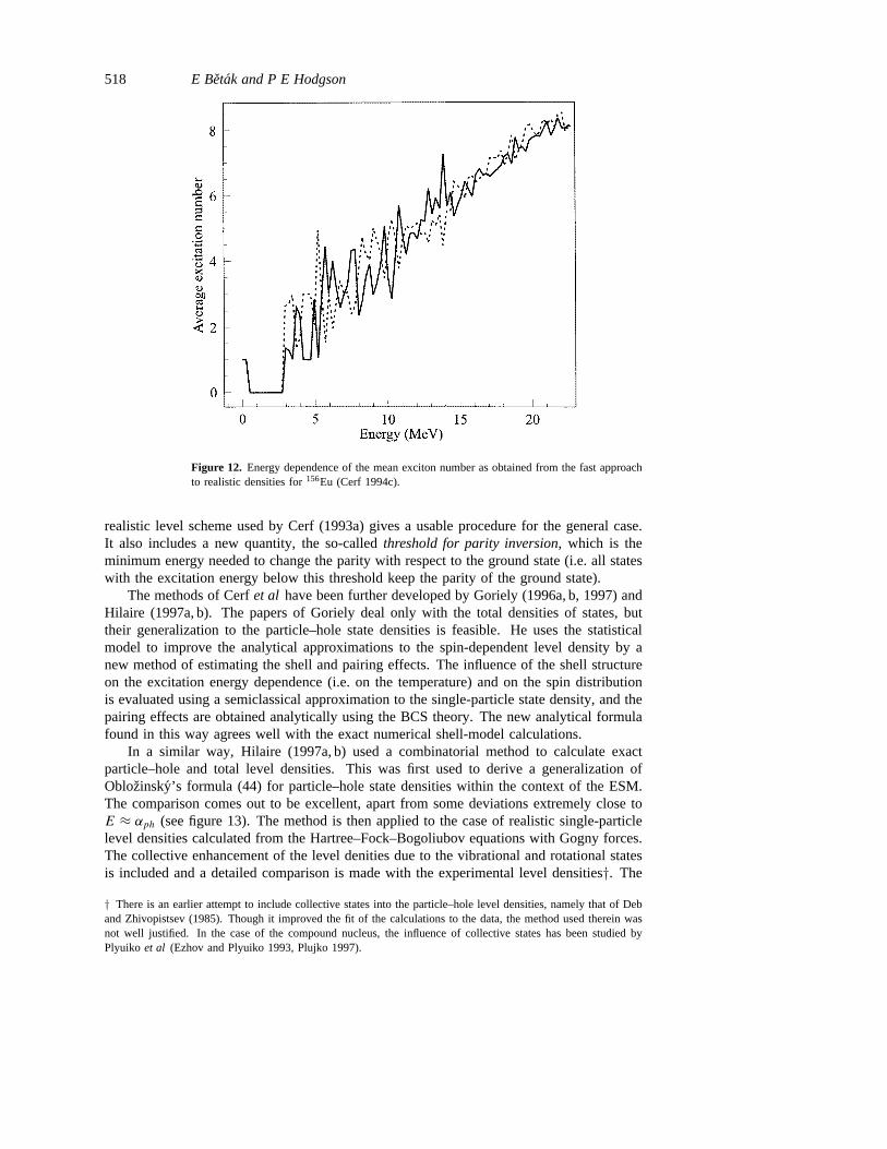
518 E Betak and P E Hodgson
Figure 12. Energy dependence of the mean exciton number as obtained from the fast approachto realistic densities for156Eu (Cerf 1994c).
realistic level scheme used by Cerf (1993a) gives a usable procedure for the general case.It also includes a new quantity, the so-calledthreshold for parity inversion, which is theminimum energy needed to change the parity with respect to the ground state (i.e. all stateswith the excitation energy below this threshold keep the parity of the ground state).
The methods of Cerfet al have been further developed by Goriely (1996a, b, 1997) andHilaire (1997a, b). The papers of Goriely deal only with the total densities of states, buttheir generalization to the particle–hole state densities is feasible. He uses the statisticalmodel to improve the analytical approximations to the spin-dependent level density by anew method of estimating the shell and pairing effects. The influence of the shell structureon the excitation energy dependence (i.e. on the temperature) and on the spin distributionis evaluated using a semiclassical approximation to the single-particle state density, and thepairing effects are obtained analytically using the BCS theory. The new analytical formulafound in this way agrees well with the exact numerical shell-model calculations.
In a similar way, Hilaire (1997a, b) used a combinatorial method to calculate exactparticle–hole and total level densities. This was first used to derive a generalization ofOblozinsky’s formula (44) for particle–hole state densities within the context of the ESM.The comparison comes out to be excellent, apart from some deviations extremely close toE ≈ αph (see figure 13). The method is then applied to the case of realistic single-particlelevel densities calculated from the Hartree–Fock–Bogoliubov equations with Gogny forces.The collective enhancement of the level denities due to the vibrational and rotational statesis included and a detailed comparison is made with the experimental level densities†. The
† There is an earlier attempt to include collective states into the particle–hole level densities, namely that of Deband Zhivopistsev (1985). Though it improved the fit of the calculations to the data, the method used therein wasnot well justified. In the case of the compound nucleus, the influence of collective states has been studied byPlyuiko et al (Ezhov and Plyuiko 1993, Plujko 1997).
Particle–hole state densities 519
Figure 13. Comparison of the energy dependence of the exact state densities (within the ESM)and those from (42) for the 32-exciton configuration (16p16h) in 208Pb. One must bear in mindthat the mean exciton numbern corresponding to the maximal energy considered isn = 20for energy of 350 (dimensionless units, which are used throughout this figure) andn = 13 forthe energy of 150 (dimensionless units), which is much in excess of the exciton configurationconsidered here (Hilaire 1997a).
energy dependence of the level density parameter is found to be well represented by theformula of Ignatyuket al (1975) provided this is modified so that the asymptotic leveldensity parameter behaves asA/13 and notA/8 and to account for the slower vanishingof the shell effects with increasing energy.
6. Conclusions
Particle–hole state and level densities are extensively used in calculations of the crosssections of pre-equilibrium reactions (Gadioli and Hodgson 1992). These calculationsrequire a knowledge of the contributing reaction mechanisms, the optical potentials thatgive the wavefunctions of the incoming and outgoing particles, and the effective nucleon–nucleon interaction as well as the particle–hole densities. There is consequently considerableflexibility in the calculations, and this has often made it possible to obtain good fits tosome rather limited data with very simplified assumptions and an inadequate understandingof the reaction mechanisms. Many pre-equilibrium reactions have contributions from themultistep compound and the multistep direct reaction mechanisms, and the cross-setionsmay also have substantial collective and compound-nucleus components. Omission of oneor more of these processes vitiated many early analyses, but now the way to calculate themis quite well understood (Demetriouet al 1996, Marcinkowskiet al 1998, Hodgson 1995,1996a, b).
For accurate calculations it is thus now necessary to refine the other parts of the calcu-lation. The optical potentials are usually taken from existing analyses of elastic scatteringat similar energies by the same or nearby nuclei. It is, however, desirable to check theirvalidity by analysing data for several reactions over a range of incident energies. The effec-tive nucleon–nucleon interaction is usually taken to have the simple zero-range or Yukawaform, but now the inclusion of analysing power data requires a spin-dependent interaction.Work is in progress using phenomenological forms and also effective interactions obtainedfrom more fundamentalG-matrix formalism (Lindsay 1995, Richter 1997).
520 E Betak and P E Hodgson
In most analyses the particle–hole level densities have been taken to have the Williamsform (21) with refinements by Betak and Dobes (1976) and Oblozinsky (1986). The recentwork of Koning and Chadwick (1997) and that of Marcinkowskiet al (1998) show thatit is necessary to use a two-fermion theory, distinguishing between neutrons and protons.More sophisticated formulae will only be used if it is no longer possible to fit the data withthe simpler ones, or if it is possible to use the better formula without too much difficulty.At present, the simpler formulae are adequate for most cases. Though in some specialcases, for example calculations of reactions to discrete states, this is no longer the case(e.g. transitions leading to discrete states calculated within the pre-equilibrium theory). Thebetter formulae frequently require very large computing times, but this difficulty may beovercome by using the techniques of Cerf (1993a, b, 1994a, b and Cerfet al (1994), Goriely(1996a, b, 1997) and Hilaire (1997a, b)). This will make it possible to study the usefulnessof the more sophisticated expressions for particle–hole state and level densities.
Recently, the International Atomic Energy Agency has prepared a document (RIPL1997/8), which recommends a suitable set of parameters and approaches to be used fornuclear reaction calculations, including a short section on the particle–hole level densities.It includes the tools for the comparison of various expressions used for the particle–hole leveldensities in pre-equilibrium calculations and a possibility to calculate them in a microscopictheory using a realistic scheme of single-particle levels.
Acknowledgments
This work has been supported in part by the Slovak Academy of Sciences grant no 1153/97and by the International Atomic Energy Agency contract no 7811/RB. EB is greatly indebtedto The Royal Society for its support and to the University of Oxford for warm hospitality.
References
Agassi D, Weidenmuller H A and Mantzouranis G 1975Phys. Rep.C 22 145Albrecht K and Blann M 1973Phys. Rev.C 8 1481Antal´ik R 1982 Neutron induced reactionsProc. Europhys. Topical Conf. (June 21–25, Smolenice)ed p Oblozinsky
(Bratislava: Inst. Phys. SAS) p 357Anzaldo-Meneses A 1995Z. Phys.A 353 295——1997Ann. Phys., Lpz.6 68Avrigeanu M and Avrigeanu V 1989J. Phys. G: Nucl. Part. Phys.15 L261——1994J. Phys. G: Nucl. Part. Phys.20 613Avrigeanu M, Harangozo A, Avrigeanu V and Antonov A N 1996 Phys. Rev.C 54 2538Avrigeanu M, Harangozo A, Stet¸cu I and Avrigeanu V 1997Int. Conf. on Nuclear Data for Science and Technology
(Trieste, May)to be published and Abstract no 106 (Abstract book, pp 93–94)Baguer N, Capote R and Pedrosa R 1989Z. Phys.A 334 397Berger J F and Martinot M 1974Nucl. Phys.A 226 391Betak E 1975Acta Phys. Slov.25 264Betak E and Dobes J 1976Z. Phys.A 279 319——1979Acta Phys. Slov.29 76Betak E, Oblozinsky P and Ribansky I 1974 Nukleonika19 687Betak E and Polhorsky V 1988 ReportINDC(CSR)-014/GJ (Vienna: IAEA)Bethe H A 1936Phys. Rev.50 332——1937Rev. Mod. Phys.9 69Birattari C, Gadioli E, Gadioli-Erba E, Grassi Strini A M, Strini G and Tagliaferri G 1973Nucl. Phys.A 201 579Blann M 1971Phys. Rev. Lett.27 337——1971Phys. Rev. Lett.27 E700——1971Phys. Rev. Lett.27 E1550——1972Phys. Rev. Lett.28 757
Particle–hole state densities 521
——1973Nucl. Phys.A 213 570——1974ReportUR-NSRL-92 (COO-3494-13) (Rochester: University of Rochester Press)——1975Annu. Rev. Nucl. Sci.25 123——1992 Nuclear Level Densities (Bologna 1989)ed G Reffo, M Herman and G Maino (Singapore: World
Scientific) p 103Blann M and Chadwick M B 1998 Phys. Rev.C 57 233Blann M, Grimes S M, Hansen L F, Komoto T T, Pohl B A, Scobel W, Trabandt M and Wong C 1985Phys. Rev.
C 32 411Blann M and Mignerey A 1972Nucl. Phys.A 186 245Blekhman A M, Duisebaev A D, Kanashevich V I and Lichman V A 1983 Report6-83 (Alma-Ata: Inst. Nucl.
Phys. Acad. Sci. KaSSR)Blin A H, Hasse R W, Hiller B, Schuck P and Yannouleas C 1986Nucl. Phys.A 456 109Blin A H, Hiller B, Hasse R W and Schuck P 1984J. Physique45 C6-231Bogila Ye A, Kolomietz V M and Sanzhur A I 1992 Z. Phys.A 341 373Bogila Ye A, Kolomietz V M, Sanzhur A I and Shlomo S 1995aZ. Phys.A 353 27——1995bPhys. Rev. Lett.75 2284Bogila Ye A, Kolomietz V M and Sanzhur A I 1996a Yad. Fiz.59 808 (Engl transl. 1996Phys. Atom. Nucl.59
770)Bogila Ye A, Kolomietz V M, Sanzhur A I and Shlomo S 1996bPhys. Rev.C 53 855Bohr A and Mottelson B 1969Nuclear Structurevol I (New York: Benjamin)Bohning M 1970Nucl. Phys.A 152 529Braga-Marcazzan G M, Gadioli-Erba E, Milazzo-Colli L and Sona P G 1972Phys. Rev.C 6 1398Burtebaev N T, Duisebaev A D, Ivanov G N, Kanashevich V I, Kabin E J, Laptev S V, Lichman V A, Nechaev
Yu I, Sukharevskii V G and Khaimin V A 1978 Izv. AN KazSSR6 19Burtebaev N T, Duisebaev A D, Ivanov G N, Kanashevich V I, Kabin E J, Lichman V A, Nechaev Yu I,
Sukharevskii V G and Khaimin V A 1982 Yad. Fiz.36 19 (Engl. transl. 1982Sov. J. Nucl. Phys.26 11)Capote R, Osorio V, Lopez R, Herrera E and Kebin E I 1987Nucleus3 1Capote Noy R, Piris Silvera M and Pedrosa Martinez R 1994 Nuclear data for science and technologyProc. Int.
Conf. (Gatlinburg, TN, May 9–13)ed J K Dickens (Oak Ridge, FL: ORNL) p 490Capote R, Ventura A and Maino G 1997Int. Conf. on Nuclear Data for Science and Technology (Trieste, May)to
be published and Abstract no 407 (Abstract book, p 111)Cerf N 1993aNucl. Phys.A 554 85——1993bNucl. Phys.A 564 383——1994aPhys. Rev.C 49 852——1994bPhys. Rev.C 50 836——1994c Private communicationCerf N, Pichon B, Rayet M and Arnould M 1994 Nuclear Data for Science and technologyProc. Int. Conf.
(Gatlinburg, TN, May 9–13)ed J K Dickens (Oak Ridge, FL: ORNL) P 479Chadwick M B and Oblozinsky P 1991Phys. Rev.C 44 R1740——1992Phys. Rev.C 46 2028Chatterjee A and Gupta S K 1981Z. Phys.A 301 271Cline C K 1971Nucl. Phys.A 174 73——1972aNucl. Phys.A 193 417——1972bNucl. Phys.A 195 353Deb A K and Zhivopistsev F A 1985Czech. J. Phys.B 35 935Demetriou P, Hodgson P E, Marcinkowski A and Watanabe Y 1996J. Phys. G: Nucl. Part. Phys.22 629Dilg W, Schantl W and Vonach H 1973Nucl. Phys.A 217 269Dobes J and Betak E 1976Nucl. Phys.A 272 353——1983Z. Phys.A 310 329Ericson T 1960Adv. Phys.9 425——1960Phil. Mag. Suppl.9 425Euler L 1753Opera Mathematicavol II (Berlin) p 254Ezhov S N and Plyuiko V A 1993 Izv. Ross. Akad. Nauk, Ser. Fiz.57 78 (Engl. transl. 1993Bull. Acad. Sci.,
Russia, Phys. Res.57)Facchini U and Saetta-Menichella E 1968Energ. Nucl.15 54Feshbach H 1973Proc. Int. Conf. Nucl. Phys. (Munich)vol II, ed J de Boer and H J Mang (Amsterdam: North-
Holland) p 632Feshbach H, Kerman A K and Koonin S 1980Ann. Phys., NY125 429
522 E Betak and P E Hodgson
Fu C Y 1984Nucl. Sci. Eng.86 344——1986Nucl. Sci. Eng.92 440——1992 Nuclear Level Densities (Bologna 1989)ed G Reffo, M Herman and G Maino (Singapore: World
Scientific) p 125——1994 Nuclear Data for Science and technologyProc. Int. Conf., Gatlinburg, TN, May 9–13)ed J K Dickens
(Oak Ridge, FL: ORNL) 482Gadioli E, Gadioli-Erba E and Hogan J J 1971Phys. Rev.C 16 1404Gadioli E, Gadioli-Erba E, Sajo-Bohus L and Tagliaferri G 1976Riv. Nuovo Cimento6 1Gadioli E, Gadioli-Erba E, Sona P G 1973Nucl. Phys.A 217 589Gadioli E and Hodgson P E 1992Pre-equilibrium Nuclear Reactions(Oxford: Clarendon)Gadioli-Erba E and Sona P G 1973 Private communication (cited in Colli M and Marcazzan B 1973)Galkin V Ya, Ishkhanov B S and Orlik S I 1979Evaluation and Interpretation of Physical Experiments(Moscow:
Moscow Univ. Publ. House) p 100 (in Russian)Galkin V Ya, Orlik S I and Orlin V N 1980 Evaluation and Interpretation of Physical Experiments(Moscow:
Moscow Univ. Publ. House) p 84 (in Russian)——1984Mathematical Problems of the Evaluation of Experiment(Moscow: Moscow Univ. Publ. House) p 110
(in Russian)Gardner D G and Gardner M A 1989 LLL Annual ReportUCRL-10002-09 (Livermore: Lawrence Livermore
Laboratory) p 47Ghosh G, Hasse R W, Schuck P and Winter J 1983Phys. Rev. Lett.50 1250Giardina G, Herman M, Italiano A, Reffo G and Rosetti M 1992Nuclear Level Densities, Bologna 1989ed G Reffo,
M Herman and G Maino (Singapore: World Scientific) p 139Gilbert A and Cameron A G W 1965Can. J. Phys.43 1446GmucaS and Ribansky I 1980 Neutron induced reactionsProc. 2nd Int. Symp. (June 25–29, 1979, Smolenice)ed
I Ribansky and E Betak (Bratislava: VEDA) p 155Goriely S 1996aNucl. Phys.A 605 28Goriely S 1996b9th Int. Symp. on Capture Gamma Ray Spectroscopy and Related Topics (Budapest, October)to
be published——1997 Int. Conf. on Nuclear Data for Science and Technology (Trieste, May)to be published and Abstract
(Abstract book, p 100)Griffin J J 1966Phys. Rev. Lett.17 478Grimes S M, Anderson J D, McClure J W, Pohl B A and Wong C 1973aPhys. Rev.C 7 343Grimes S M, Anderson J D, Davis J C and Wong C 1973bPhys. Rev.C 8 1770Grimes S M, Anderson J D and Wong C 1976Phys. Rev.C 13 2224Gruppelaar H, Nagel P and Hodgson P E 1986Riv. Nuovo Cimento9Gudima K K, Mashnik S G and Toneev V D 1983 Nucl. Phys.A 401 329Gupta S K 1981Z. Phys.A 303 329Hasse R W 1985/86Ann. Univ. M. Curie-Sklodowska, sect. AAAXL/XLI 16 191Herman M and Reffo G 1987aComput. Phys. Commun.47 103——1987bPhys. Rev.C 36 1546——1992 Nuclear Level Densities (Bologna 1989)ed G Reffo, M Herman and G Maino (Singapore: World
Scientific) p 103Herman M, Reffo G and Costa C 1989Phys. Rev.C 39 1269Herman M, Reffo G and Rego R A 1988Phys. Rev.C 37 797Herman M, Reffo G and Weidenmuller H A 1992 Nucl. Phys.A 536 124Hilaire S 1997aSpecialists’ Meeting on Nucleon–nucleus Optical Model up to 200 MeV (Bruy`eres-le-Chˆatel,
November 1996), ReportNEA No 0293 (Paris: NEA)——1997b Int. Conf. on Nuclear Data for Science and Technology (Trieste, May)to be published and Abstract
no 268 (Abstract book, p 104)Hillman M and Grover J R 1969Phys. Rev.185 1303Hodgson P E 1995Acta Phys. Hung. N.S., Heavy Ion Physics2 175——1996a Proc. Int. Nuclear Physics Conf.—NPC ’95ed Sun Zuxun and Xu Jincheng (Singapore: World
Scientific) p 426——1996bProc. XV RCNP Osaka Int. Symp. on Nuclear Physics(Singapore: World Scientific) p 361Ignatyuk A V 1973 Yad. Fiz.17 502 (Engl. transl. 1973Sov. J. Nucl. Phys.17 258)——1983 Statisticheskiye svoistva vozbuzhdennykh atomnykh yader(Moscow: Energoatomizdat) (Engl. transl.
1985 Statistical properties of excited atomic nucleiReportINDC(CCP)-233/L (Vienna: Int. Atomic EnergyAgency))
Particle–hole state densities 523
Ignatyuk A V, Smirenkin G N and Tishin A S 1975Yad. Fiz.21 485 (Engl. transl. 1975Sov. J. Nucl. Phys.21255)
Ignatyuk A V and Sokolov Yu V 1972Yad. Fiz.16 277 (Engl. transl. 1973Sov. J. Nucl. Phys.16 155)——1973Yad. Fiz.17 723 (Engl. transl. 1973Sov. J. Nucl. Phys.17 376)——1978Yad. Fiz.28 914 (Engl. transl. 1978Sov. J. Nucl. Phys.28 469)Iljinov A S, Mebel M V, Bianchi N, De Sancti S E, Lucheroni V, Muccifora W, Polli E, Reolin A R and Rossi P
1992Nucl. Phys.A 543 517Isaev P N 1985Preprint 85-25 (Novosibirsk: Inst. Nucl. Phys. Acad. Sci. USSR)Jacquemin C and Kataria S K 1986Z. Phys.A 324 261Jensen J H D andLuttingen J M 1952Phys. Rev.86 907Jingshang Zhang 1994Chin. J. Nucl. Phys.16 55Kalbach C 1975Nuovo CimentoA 29 283——1977Z. Phys.A 283 401——1981Phys. Rev.C 24 819——1984Phys. Rev.C 30 1310——1985Phys. Rev.C 32 1157——1986Phys. Rev.C 33 818——1987Nucl. Sci. Eng.95 70——1989Z. Phys.A 332 157——1993Phys. Rev.C 47 587——1995aJ. Phys. G: Nucl. Part. Phys.21 1499——1995bJ. Phys. G: Nucl. Part. Phys.21 1519——1995cActa Phys. Slov.45 685Kalbach-Cline C, Huizenga J R and Vonach H K 1974Nucl. Phys.A 222 405Kikuchi K and Kawai M 1968Nuclear Matter and Nuclear Reactions(Amsterdam: North-Holland)Koning A J and Chadwick M B 1997 Phys. Rev.C 56 970Lee E V and Griffin J J 1972Phys. Rev.C 5 1713Lindsay R 1995Acta Phys. Slov.45 717Madler P and Reif R 1980Nucl. Phys.A 337 445——1982Nucl. Phys.A 373 27Madler P, Reif R and Toneev V D 1978 Report05-25-78 (Dresden: Technical University, Sect. Physics)Mao Ming De and Guo Hua 1993J. Phys. G: Nucl. Part. Phys.19 421Marcinkowski A, Marianski B, Moroz Z, Wojtkowska J and Demetriou P 1998Nucl. Phys.in pressMashnik S G 1993Acta Phys. Slov.43 86Mengoni A and Nakajima Y 1994J. Nucl. Sci. Technol.31 151Moretto L G 1975Nucl. Phys.A 243 77Mustafa M G, Blann M, Ignatyuk A V and Grimes S M 1992Phys. Rev.C 45 1078Munster A 1969Statistical Thermodynamicsvol I (Berlin: Springer) para 2.9Nilsson S G 1955Mat. Fys. Medd. Dansk. Vid. Selsk.29Nishioka H, Verbaarschot J J M, Weidenmuller H A and Yoshida S 1986Ann. Phys., NY172 67Nishioka H, Weidenmuller H A and Yoshida S 1988aAnn. Phys., NY183 166——1988bPhys. Lett.203B 1——1989Ann. Phys., NY193 195Oblozinsky P 1986Nucl. Phys.A 453 127——1987Phys. Rev.C 35 407——1990Phys. Rev.C 41 401Oblozinsky P and Chadwick M B 1990 Phys. Rev.C 42 1652Oblozinsky P, Ribansky I and Betak E 1974Nucl. Phys.A 226 347Orlik S I 1980Evaluation and Interpretation of Physical Experiments(Moscow: Moscow Univ. Publ. House) p 65
(in Russian)Pichon B 1994Nucl. Phys.A 568 553Plujko V 1997 Int. Conf. on Nuclear Data for Science and Technology (Trieste, May)to be published (Abstract
book, p 103)Plyuiko V A 1978 Yad. Fiz.27 1175 (Engl. transl. 1978Sov. J. Nucl. Phys.27 623)RIPL (Reference Input Parameter Library) 1997/8Handbook for Calculations of Nuclear Reaction Data(Vienna:
Int. Atomic Energy Agency) Draft 2 obtainable via ftp from iaeand.iaea.or.atReffo G and Herman M 1982Lett. Nuovo Cimento34 261Ribansky I, Oblozinsky P and Betak E 1973Nucl. Phys.A 205 545
524 E Betak and P E Hodgson
Richter W A 1997 Private communicationRohr G 1984Z. Phys.A 318 299Rosenzweig N 1957Phys. Rev.108 817Sato K and Yoshida S 1987Z. Phys.A 327 421——1988Z. Phys.A 330 265——1989Z. Phys.A 333 141——1992Nuclear Level Densities (Bologna 1989)ed G Reffoet al (Singapore: World Scientific) p 113——1994Phys. Rev.C 49 1099Sato K, Takahashi Y and Yoshida S 1991Z. Phys.A 339 129——1992Nuclear Level Densities (Bologna 1989)ed G Reffoet al (Singapore: World Scientific) p 147Scobel W, Blann M, Komoto T T, Trabandt M, Grimes S M, Hansen L F, Wong C and Pohl B A 1984 Phys. Rev.
C 30 1480Seeger P A and Howard V M 1975 Nucl. Phys.A 238 491Seeger P A and Perisho R C 1967ReportLA-3751 (Los Alamos, NM: LANL)Shi Xiangjun, Gruppelaar H and Akkermans J M 1987Nucl. Phys.A 466 333Shlomo S 1992Nucl. Phys.A 539 17Shlomo S, Bogila Ye A, Kolomietz V M and Sanzhur A I 1995 Z. Phys.A 353 27Shlomo S, Kolomietz V M and Dejbakhsh 1997Phys. Rev.C 55 1972Sokolov Yu V 1972Yad. Fiz.16 27 (Engl. transl. 1972Sov. J. Nucl. Phys.16 14)Smith R D 1989ReportLAUR-97-2930 (Los Alamos, NM: LANL)Stankiewicz K, Marcinkowski A and Herman M 1985Nucl. Phys.A 435 67Strutinski V 1959Congres Int. de Physique Nucl´eaire (Paris 1958)ed P Gugenberger (Paris: Dunod) p 617Tamura T, Udagawa T and Lenske H 1982Phys. Rev.C 26 1033Williams F C Jr1970Phys. Lett.B 31 184——1971Nucl. Phys.A 166 231Williams F C Jr, Mignerey A and Blann M 1973Nucl. Phys.A 207 619Woods R D and Saxon D S 1954Phys. Rev.95 577Yoshida S, Abe M and Sato K 1995Acta Phys. Slov.45 757Zhang J 1990ReportINDC(CRP)-017/LJ (Vienna: IAEA)——1993Nucl. Sci. Eng.114 55Zhang J S and Wu S 1992aZ. Phys.A 344 49Zhang Jingshang and Wu Shunguang 1992bChin. J. Nucl. Phys.14 121Zhang J S and Yang X J 1988Z. Phys.A 329 69Zhivopistsev F A, Lukashev A V and Shitikova K V 1973 Izv. AN SSSR, Ser. Phys.37 2634Zhivopistsev F A, Kabin E J, Sukharevskii V G and Khaimin V A 1982 Izv. AN SSSR, Ser. Phys.46 885Zhivopistsev F A, Kabin E J and Sukharevskii V G 1987 Models of Pre-equilibrium Reactions(Moscow: MGU
Publ. House) (in Russian)