Particle Acceleration

USPAS, January 2014

Lecture 2

Outline

• Electrostatic accelerators

• Radio-frequency (RF) linear accelerators

• RF Cavities and their properties

• Material is covered in Wiedemann Chapter

15 (and also in Wangler, Chapter 1)

How do we accelerate particles?

• We can accelerate charged particles:

– electrons (e-) and positrons (e+)

– protons (p) and antiprotons (p-bar)

– Ions (e.g. H1-, Ne2+, Au92+ , …)

• These particles are typically “born” at low-

energy

– e- : emission from thermionic gun at ~100 kV

– p/ions: sources at ~50 kV

• The application usually requires that we

accelerate these particles to higher energy, in

order to make use of them

Electromagnetic Forces on Charged Particles

• Lorentz force equation gives the force in response to electric

and magnetic fields:

• The equation of motion becomes:

• The kinetic energy of a charged particle increases by an

amount equal to the work done (Work-Energy Theorem)

ldBvqldEqldFW

)(

ldEqdtvBvqldEqW

)(

Electromagnetic Forces on Charged Particles

• We therefore reach the important conclusion that – Magnetic fields cannot be used to change the kinetic

energy of a particle

• We must rely on electric fields for particle acceleration – Acceleration occurs along the direction of the electric

field

– Energy gain is independent of the particle velocity

• In accelerators: – Longitudinal electric fields (along the direction of

particle motion) are used for acceleration

– Magnetic fields are used to bend particles for guidance and focusing

Acceleration by Static Fields:

Electrostatic Accelerators

Acceleration by Static Electric Fields

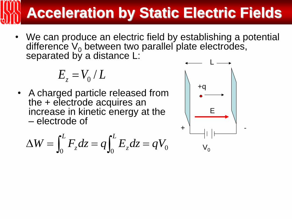
• We can produce an electric field by establishing a potential difference V0 between two parallel plate electrodes, separated by a distance L:

LVEz /0

V0

+ -

+q

L

000

qVdzEqdzFWL

z

L

z

E

• A charged particle released from the + electrode acquires an increase in kinetic energy at the – electrode of

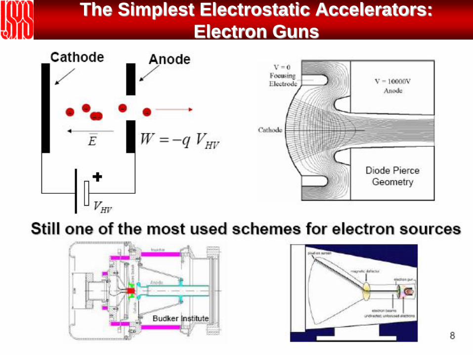
The Simplest Electrostatic Accelerators:

Electron Guns

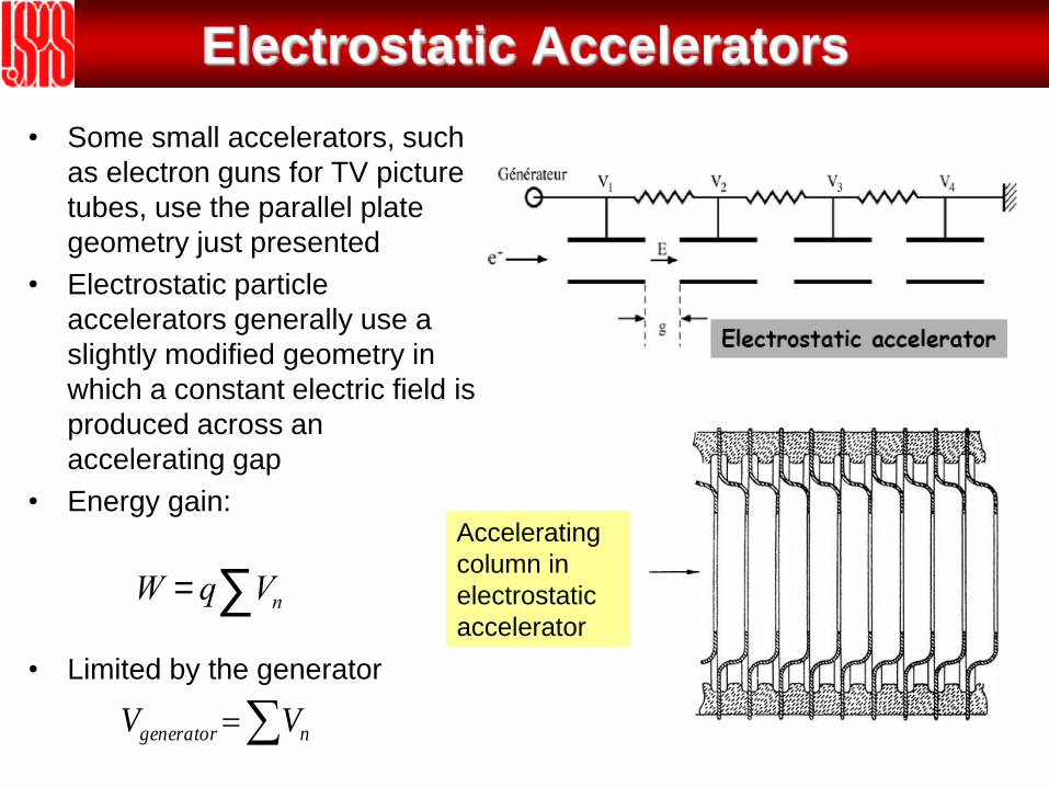
Electrostatic Accelerators

• Some small accelerators, such

as electron guns for TV picture

tubes, use the parallel plate

geometry just presented

• Electrostatic particle

accelerators generally use a

slightly modified geometry in

which a constant electric field is

produced across an

accelerating gap

• Energy gain:

• Limited by the generator

ngenerator VV

W = q Vnå

Accelerating

column in

electrostatic

accelerator

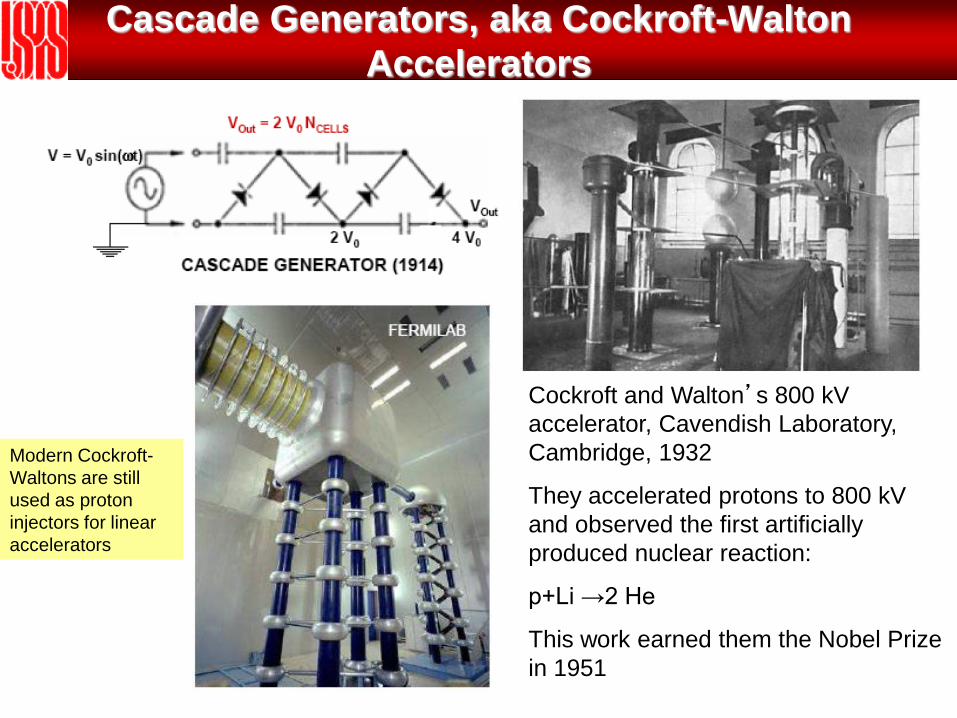
Cascade Generators, aka Cockroft-Walton

Accelerators

Cockroft and Walton’s 800 kV

accelerator, Cavendish Laboratory,

Cambridge, 1932

They accelerated protons to 800 kV

and observed the first artificially

produced nuclear reaction:

p+Li →2 He

This work earned them the Nobel Prize

in 1951

Modern Cockroft-

Waltons are still

used as proton

injectors for linear

accelerators

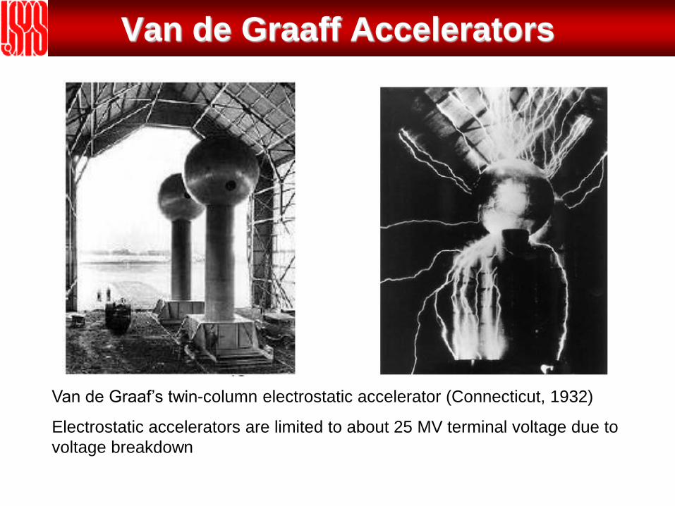
Van de Graaff Accelerators

Van de Graaf’s twin-column electrostatic accelerator (Connecticut, 1932)

Electrostatic accelerators are limited to about 25 MV terminal voltage due to

voltage breakdown

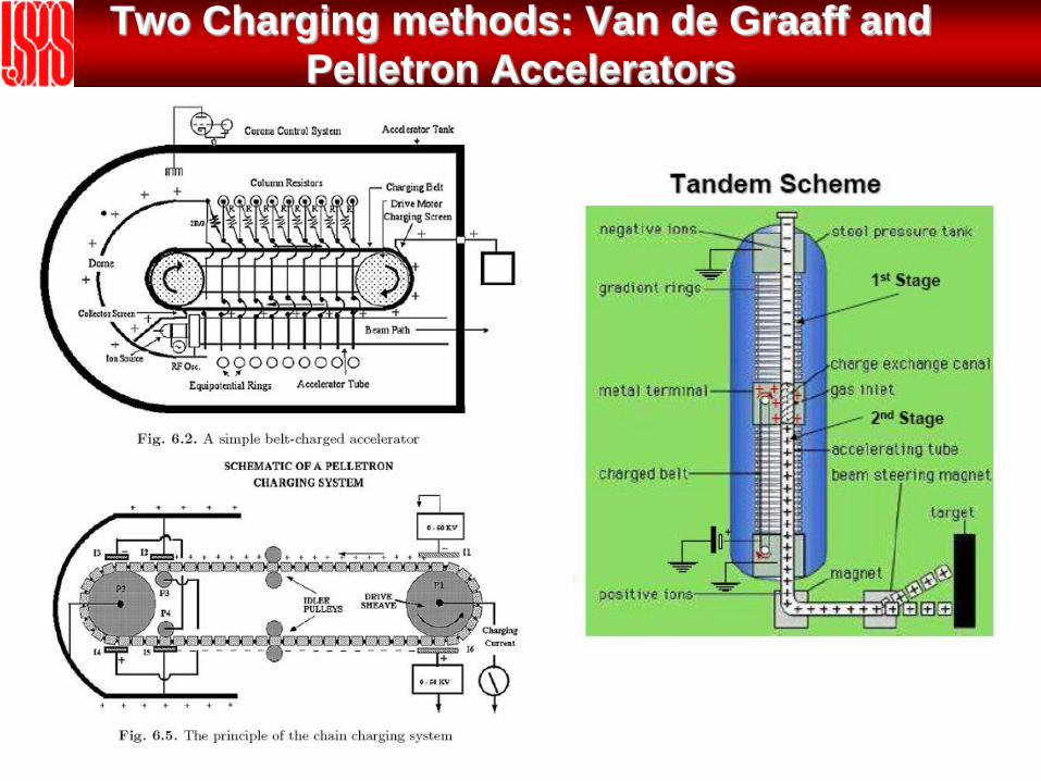
Two Charging methods: Van de Graaff and

Pelletron Accelerators

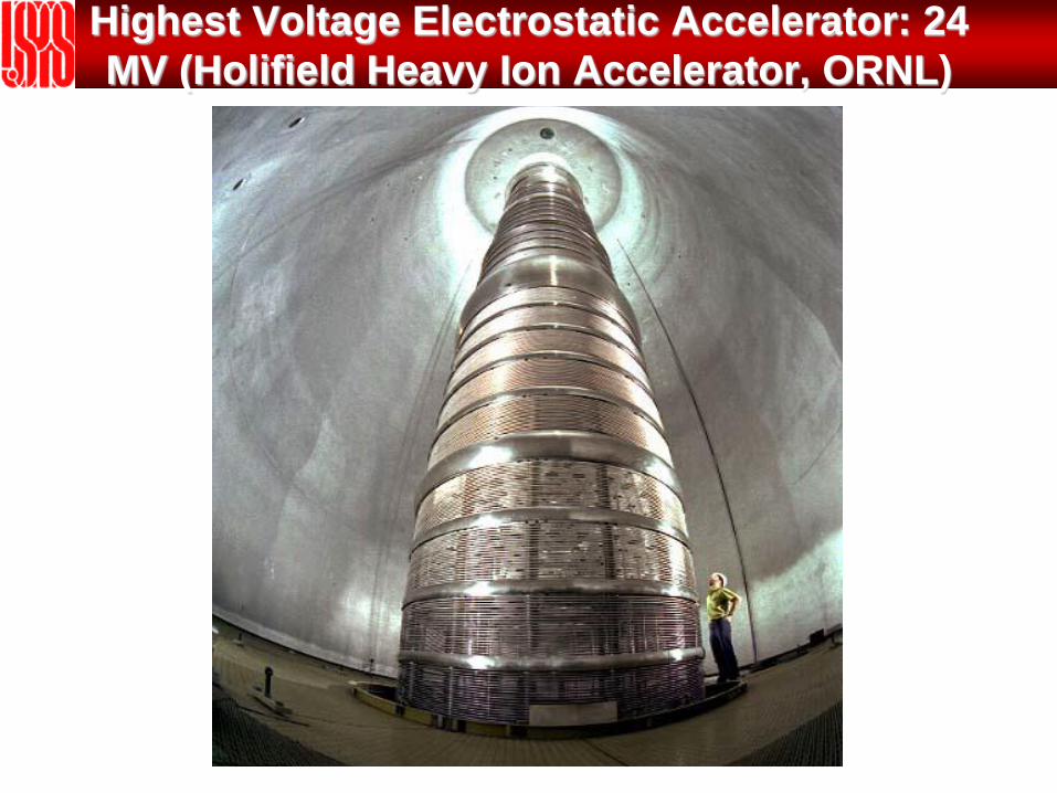
Highest Voltage Electrostatic Accelerator: 24

MV (Holifield Heavy Ion Accelerator, ORNL)

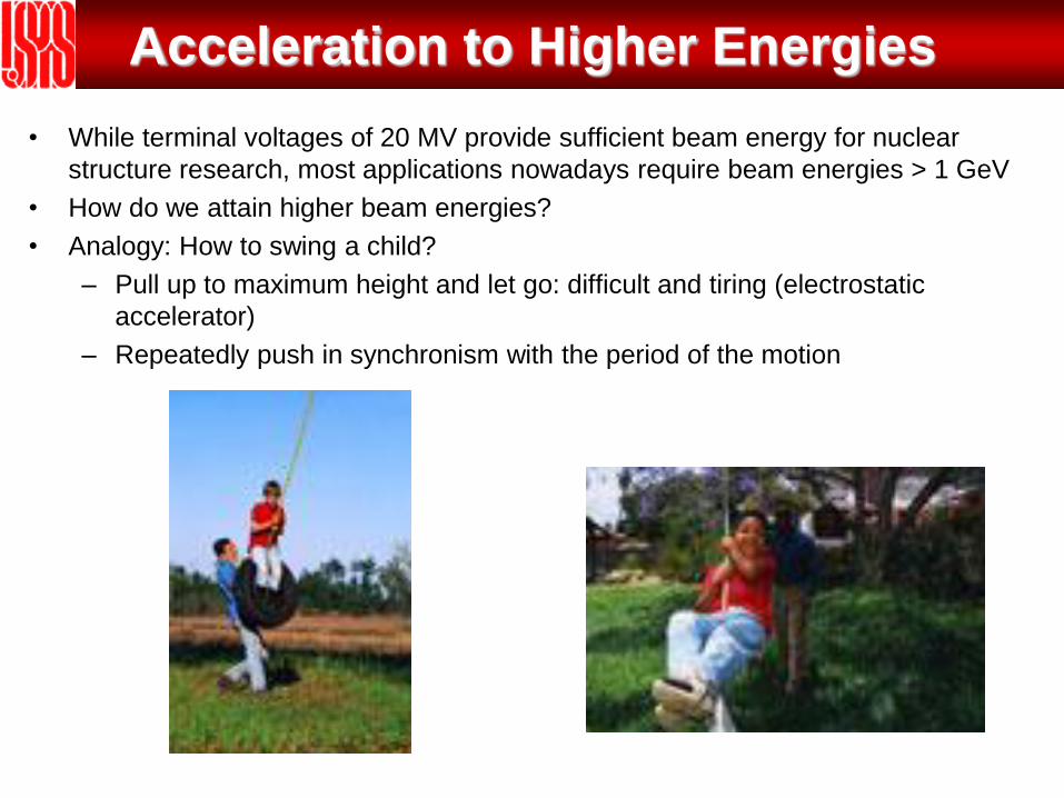
Acceleration to Higher Energies

• While terminal voltages of 20 MV provide sufficient beam energy for nuclear

structure research, most applications nowadays require beam energies > 1 GeV

• How do we attain higher beam energies?

• Analogy: How to swing a child?

– Pull up to maximum height and let go: difficult and tiring (electrostatic

accelerator)

– Repeatedly push in synchronism with the period of the motion

Acceleration by Time-Varying

Fields: Radio-Frequency

Accelerators

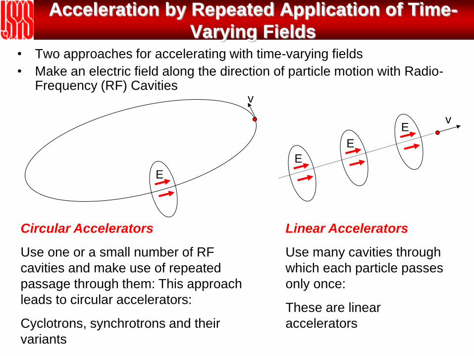
Acceleration by Repeated Application of Time-

Varying Fields • Two approaches for accelerating with time-varying fields

• Make an electric field along the direction of particle motion with Radio-Frequency (RF) Cavities

v

E

E

E

E v

Circular Accelerators

Use one or a small number of RF

cavities and make use of repeated

passage through them: This approach

leads to circular accelerators:

Cyclotrons, synchrotrons and their

variants

Linear Accelerators

Use many cavities through

which each particle passes

only once:

These are linear

accelerators

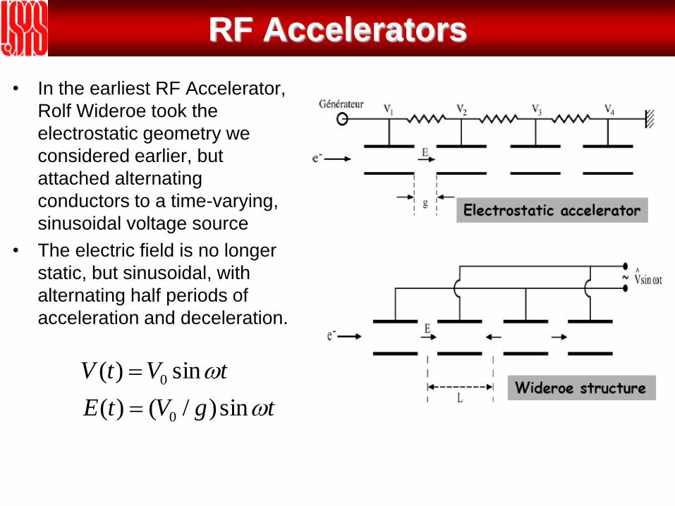
RF Accelerators

• In the earliest RF Accelerator,

Rolf Wideroe took the

electrostatic geometry we

considered earlier, but

attached alternating

conductors to a time-varying,

sinusoidal voltage source

• The electric field is no longer

static, but sinusoidal, with

alternating half periods of

acceleration and deceleration.

tgVtE

tVtV

sin)/()(

sin)(

0

0

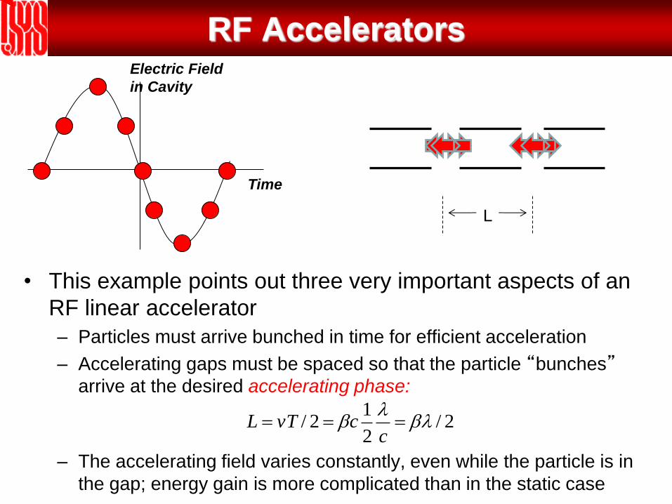
RF Accelerators

• This example points out three very important aspects of an

RF linear accelerator

– Particles must arrive bunched in time for efficient acceleration

– Accelerating gaps must be spaced so that the particle “bunches” arrive at the desired accelerating phase:

– The accelerating field varies constantly, even while the particle is in

the gap; energy gain is more complicated than in the static case

Electric Field

in Cavity

Time

2/2

12/

ccvTL

L

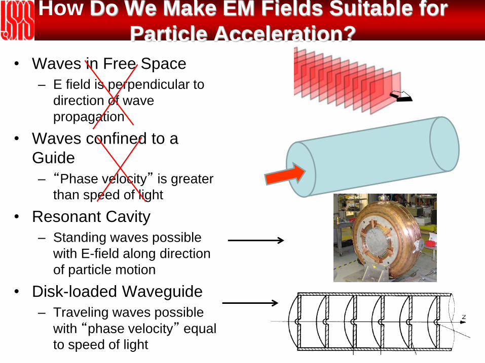
How Do We Make EM Fields Suitable for

Particle Acceleration?

• Waves in Free Space

– E field is perpendicular to

direction of wave

propagation

• Waves confined to a

Guide

– “Phase velocity” is greater

than speed of light

• Resonant Cavity

– Standing waves possible

with E-field along direction

of particle motion

• Disk-loaded Waveguide

– Traveling waves possible

with “phase velocity” equal

to speed of light

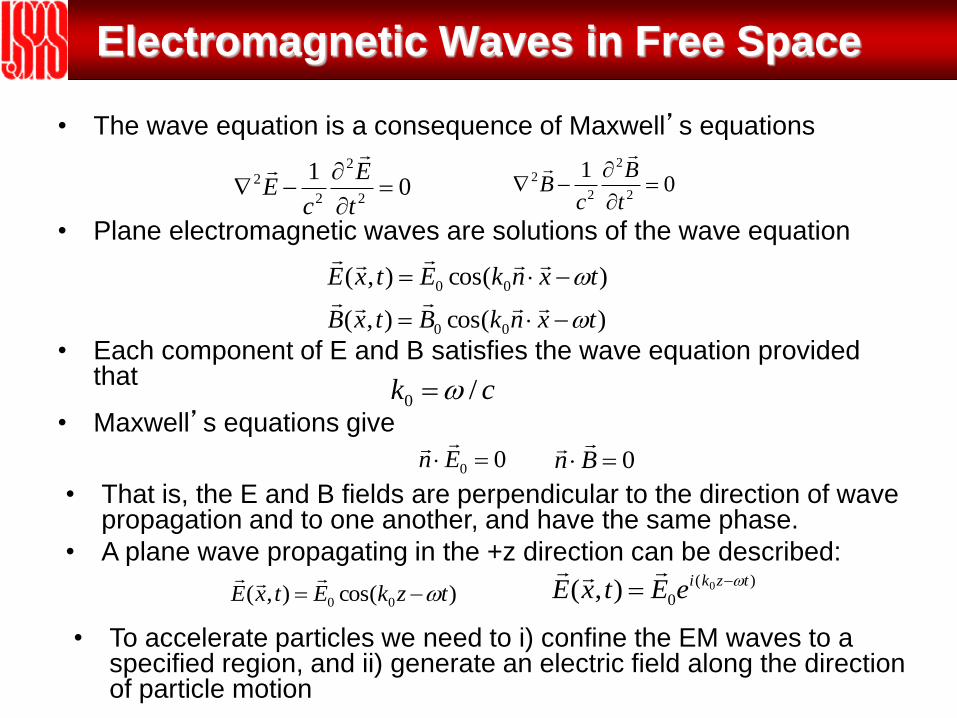
Electromagnetic Waves in Free Space

• The wave equation is a consequence of Maxwell’s equations

01

2

2

2

2

t

E

cE

01

2

2

2

2

t

B

cB

)(

00),(

tzkieEtxE

• That is, the E and B fields are perpendicular to the direction of wave propagation and to one another, and have the same phase.

• A plane wave propagating in the +z direction can be described:

• Plane electromagnetic waves are solutions of the wave equation

)cos(),(

)cos(),(

00

00

txnkBtxB

txnkEtxE

• Each component of E and B satisfies the wave equation provided that

ck /0 • Maxwell’s equations give

00 En

0Bn

• To accelerate particles we need to i) confine the EM waves to a specified region, and ii) generate an electric field along the direction of particle motion

)cos(),( 00 tzkEtxE

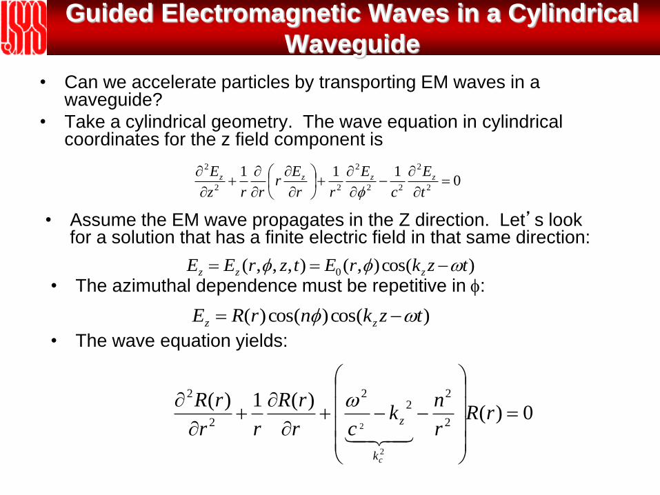
Guided Electromagnetic Waves in a Cylindrical

Waveguide

• Can we accelerate particles by transporting EM waves in a waveguide?

• Take a cylindrical geometry. The wave equation in cylindrical coordinates for the z field component is

0111

2

2

22

2

22

2

t

E

c

E

rr

Er

rrz

E zzzz

• Assume the EM wave propagates in the Z direction. Let’s look for a solution that has a finite electric field in that same direction:

)cos(),(),,,( 0 tzkrEtzrEE zzz

• The azimuthal dependence must be repetitive in :

)cos()cos()( tzknrRE zz

• The wave equation yields:

0)()(1)(

2

22

2

2

2

2

2

rR

r

nk

cr

rR

rr

rR

ck

z

Cylindrical Waveguides

0)/1(1 22

2

2

Rxndx

dR

xdx

Rd

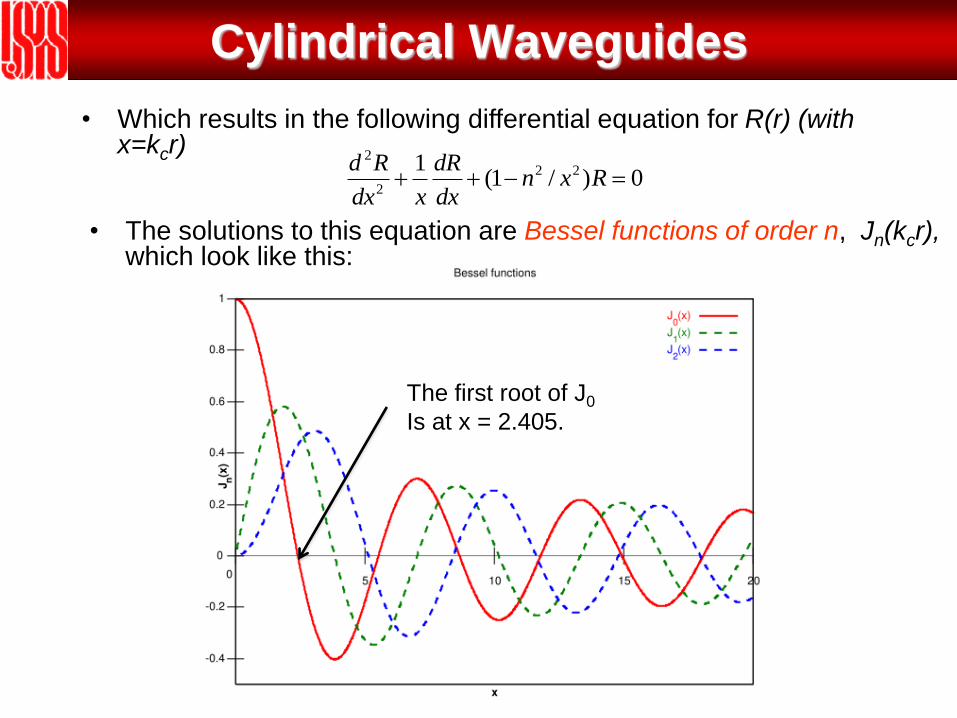
• Which results in the following differential equation for R(r) (with x=kcr)

• The solutions to this equation are Bessel functions of order n, Jn(kcr), which look like this:

The first root of J0

Is at x = 2.405.

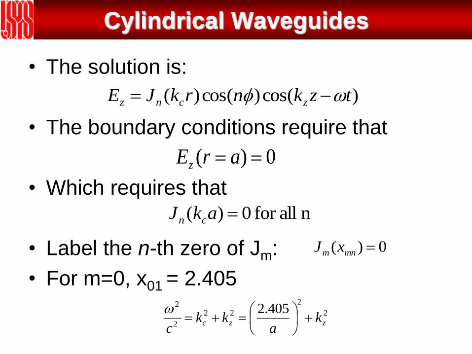
Cylindrical Waveguides

• The solution is:

• The boundary conditions require that

• Which requires that

• Label the n-th zero of Jm:

• For m=0, x01 = 2.405

)cos()cos()( tzknrkJE zcnz

0)( arEz

n allfor 0)( akJ cn

0)( mnm xJ

2

2

22

2

2 405.2zzc k

akk

c

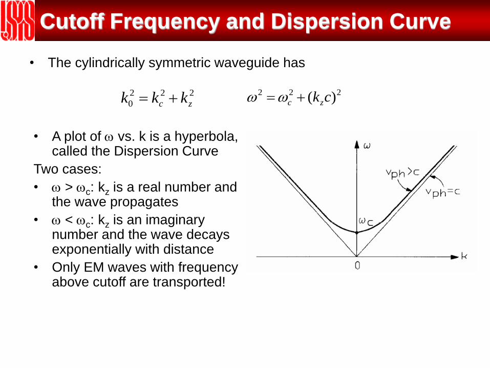
Cutoff Frequency and Dispersion Curve

222

0 zc kkk

• The cylindrically symmetric waveguide has

222 )( ckzc

• A plot of vs. k is a hyperbola, called the Dispersion Curve

Two cases:

• > c: kz is a real number and the wave propagates

• < c: kz is an imaginary number and the wave decays exponentially with distance

• Only EM waves with frequency above cutoff are transported!

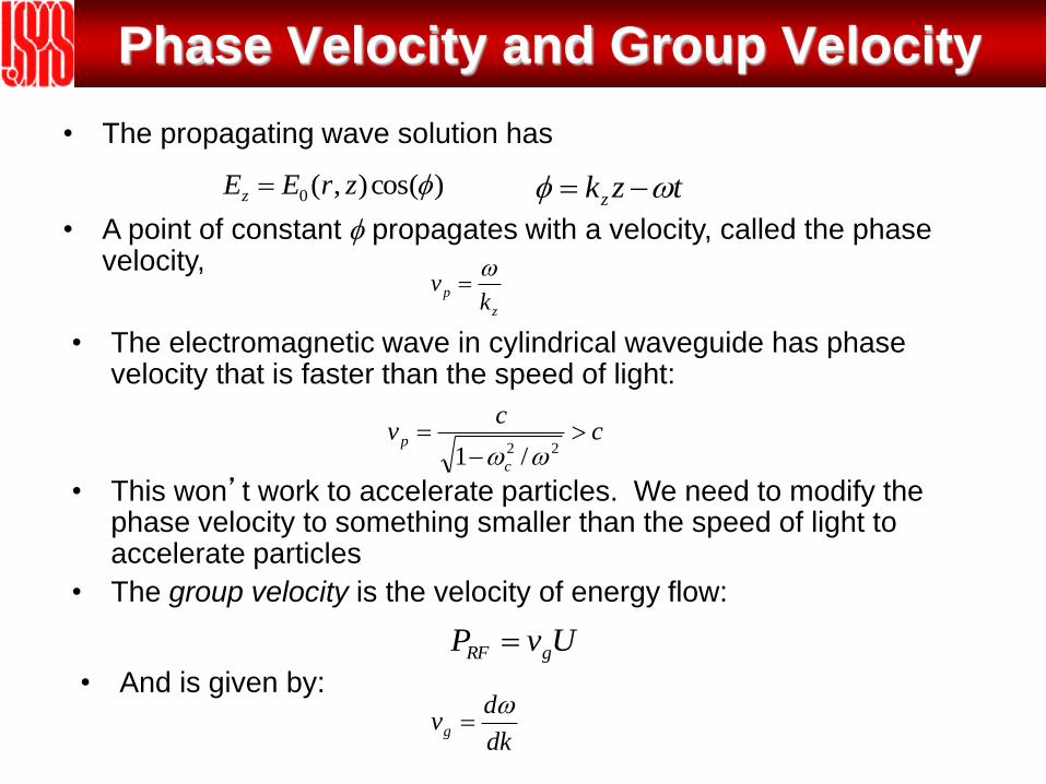
Phase Velocity and Group Velocity

• The propagating wave solution has

tzkz

cc

v

c

p

22 /1

• The electromagnetic wave in cylindrical waveguide has phase velocity that is faster than the speed of light:

• This won’t work to accelerate particles. We need to modify the phase velocity to something smaller than the speed of light to accelerate particles

• The group velocity is the velocity of energy flow:

)cos(),(0 zrEEz

• A point of constant propagates with a velocity, called the phase velocity,

z

pk

v

UvP gRF

• And is given by:

dk

dvg

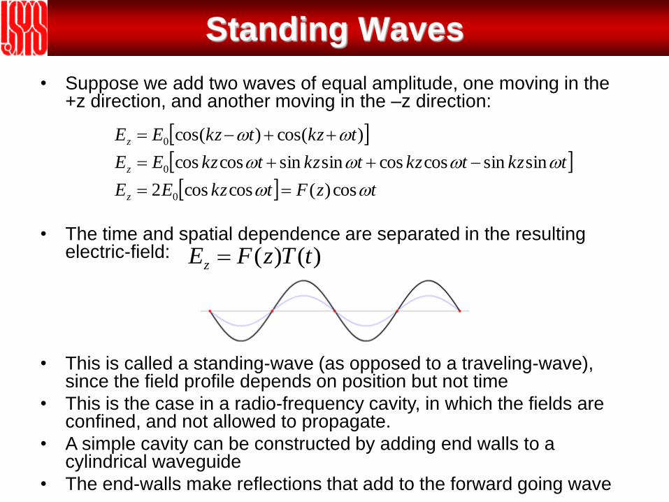
Standing Waves

• Suppose we add two waves of equal amplitude, one moving in the +z direction, and another moving in the –z direction:

tzFtkzEE

tkztkztkztkzEE

tkztkzEE

z

z

z

cos)(coscos2

sinsincoscossinsincoscos

)cos()cos(

0

0

0

• The time and spatial dependence are separated in the resulting electric-field:

• This is called a standing-wave (as opposed to a traveling-wave), since the field profile depends on position but not time

• This is the case in a radio-frequency cavity, in which the fields are confined, and not allowed to propagate.

• A simple cavity can be constructed by adding end walls to a cylindrical waveguide

• The end-walls make reflections that add to the forward going wave

)()( tTzFEz

Radio-frequency (RF) Cavities

Radio Frequency Cavities: The Pillbox Cavity

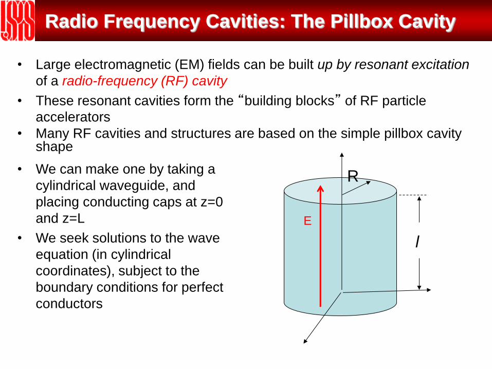
• Large electromagnetic (EM) fields can be built up by resonant excitation

of a radio-frequency (RF) cavity

• These resonant cavities form the “building blocks” of RF particle

accelerators

• Many RF cavities and structures are based on the simple pillbox cavity shape

• We can make one by taking a

cylindrical waveguide, and

placing conducting caps at z=0

and z=L

• We seek solutions to the wave

equation (in cylindrical

coordinates), subject to the

boundary conditions for perfect

conductors

R

l

E

Conducting Walls

• Boundary conditions at the vacuum-perfect conductor interface are

derived from Maxwell’s equations:

• These boundary conditions mean:

– Electric fields parallel to a metallic surface vanish at the surface

– Magnetic fields perpendicular to a metallic surface vanish at the surface

• In the pillbox-cavity case:

• For a real conductor (meaning finite conductivity) fields and currents

are not exactly zero inside the conductor, but are confined to a small

finite layer at the surface called the skin depth

• The RF surface resistance is

.2

0

2/1 0sR

0ˆ ˆ

0ˆ ˆ0

EnKHn

BnEn

RrEE

lzzEE

z

r

for 0

and 0for 0

Wave Equation in Cylindrical Coordinates

0111

2

2

22

2

22

2

t

E

c

E

rr

Er

rrz

E zzzz

trREtzrEz cos)(),,( 0

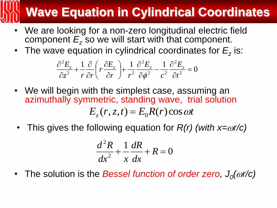
• We are looking for a non-zero longitudinal electric field component Ez so we will start with that component.

• The wave equation in cylindrical coordinates for Ez is:

• We will begin with the simplest case, assuming an azimuthally symmetric, standing wave, trial solution

• This gives the following equation for R(r) (with x=r/c)

01

2

2

Rdx

dR

xdx

Rd

• The solution is the Bessel function of order zero, J0(r/c)

Bessel Functions

Note that J0(2.405)=0

r/c

Longitudinal Electric Field

• The solution for the longitudinal electric field is

• To satisfy the boundary conditions, Ez must vanish at the

cavity radius: 0)( RrEz

• Which is only possible if the Bessel function equals zero

tcrJEEz cos)/(00

0)()/( 00 RkJcRJ rc

• Using the first zero, J0(2.405)=0, gives

Rcc /405.2

• That is, for a given radius, there is only a single frequency

which satisfies the boundary conditions

• The cavity is resonant at that frequency

Magnetic Field Component

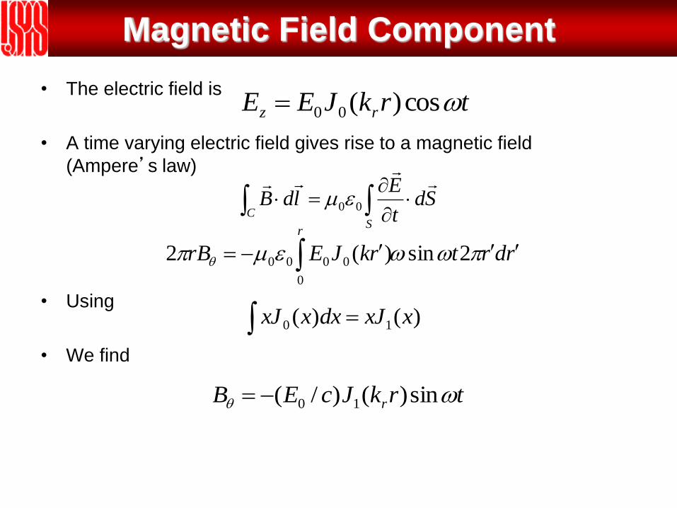
• The electric field is

• A time varying electric field gives rise to a magnetic field

(Ampere’s law)

• Using

• We find

CS

Sdt

EldB

00

rdrtrkJErB

r

2sin)(20

0000

trkJcEB r sin)()/( 10

trkJEE rz cos)(00

)()( 10 xxJdxxxJ

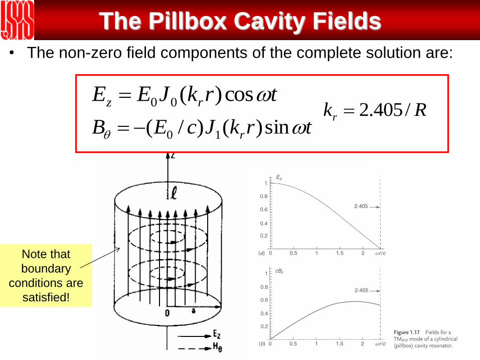
The Pillbox Cavity Fields

trkJEE rz cos)(00

trkJcEB r sin)()/( 10Rkr /405.2

• The non-zero field components of the complete solution are:

Note that

boundary

conditions are

satisfied!

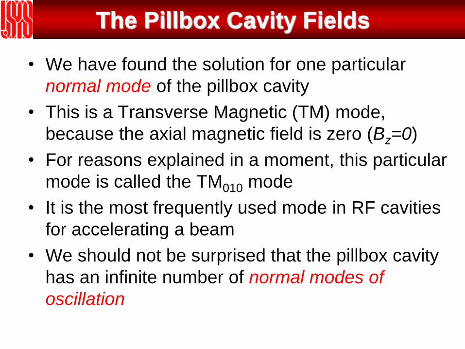
The Pillbox Cavity Fields

• We have found the solution for one particular

normal mode of the pillbox cavity

• This is a Transverse Magnetic (TM) mode,

because the axial magnetic field is zero (Bz=0)

• For reasons explained in a moment, this particular

mode is called the TM010 mode

• It is the most frequently used mode in RF cavities

for accelerating a beam

• We should not be surprised that the pillbox cavity

has an infinite number of normal modes of

oscillation

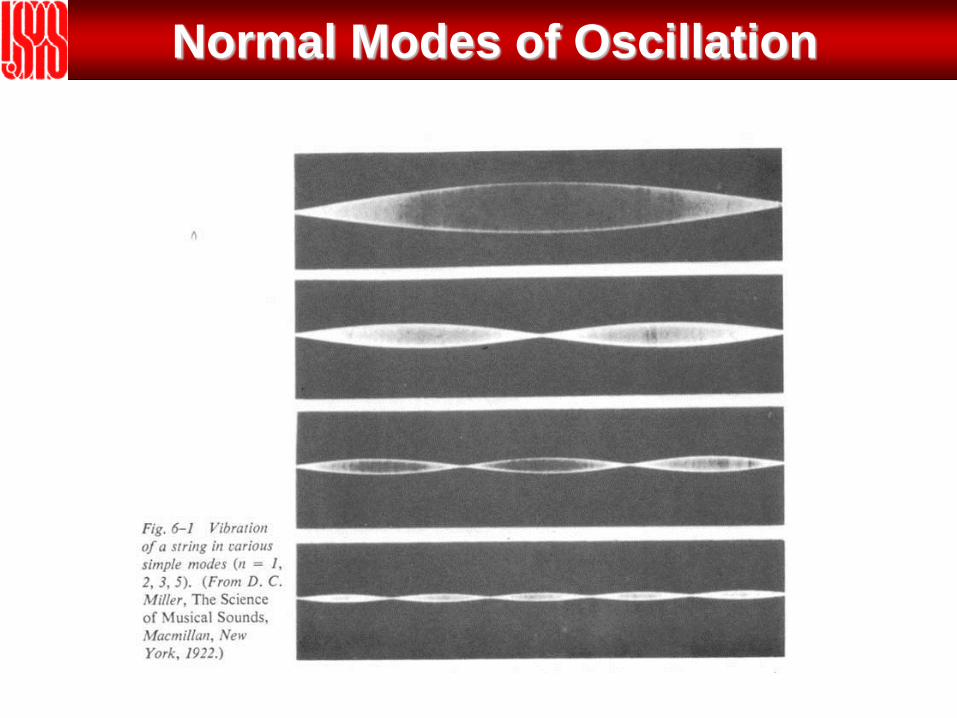
Normal Modes of Oscillation

Mechanical Normal Modes

Drumhead modes

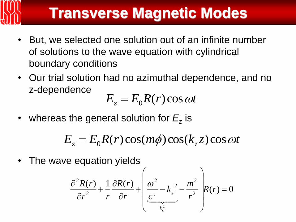
• But, we selected one solution out of an infinite number

of solutions to the wave equation with cylindrical

boundary conditions

• Our trial solution had no azimuthal dependence, and no

z-dependence

• whereas the general solution for Ez is

• The wave equation yields

trREEz cos)(0

tzkmrREE zz cos)cos()cos()(0

Transverse Magnetic Modes

0)()(1)(

2

22

2

2

2

2

2

rR

r

mk

cr

rR

rr

rR

ck

z

Transverse Magnetic Modes

• Which results in the following differential equation

for R(r) (with x=kcr)

• With solutions Jm(kcr), Bessel functions of order m

• The solution is:

• The boundary conditions require that

• Which requires that

0)/1(1 22

2

2

Rxmdx

dR

xdx

Rd

tzkmrkJEE zcmz cos)cos()cos()(0

m allfor 0)( RkJ cm

0)( RrEz

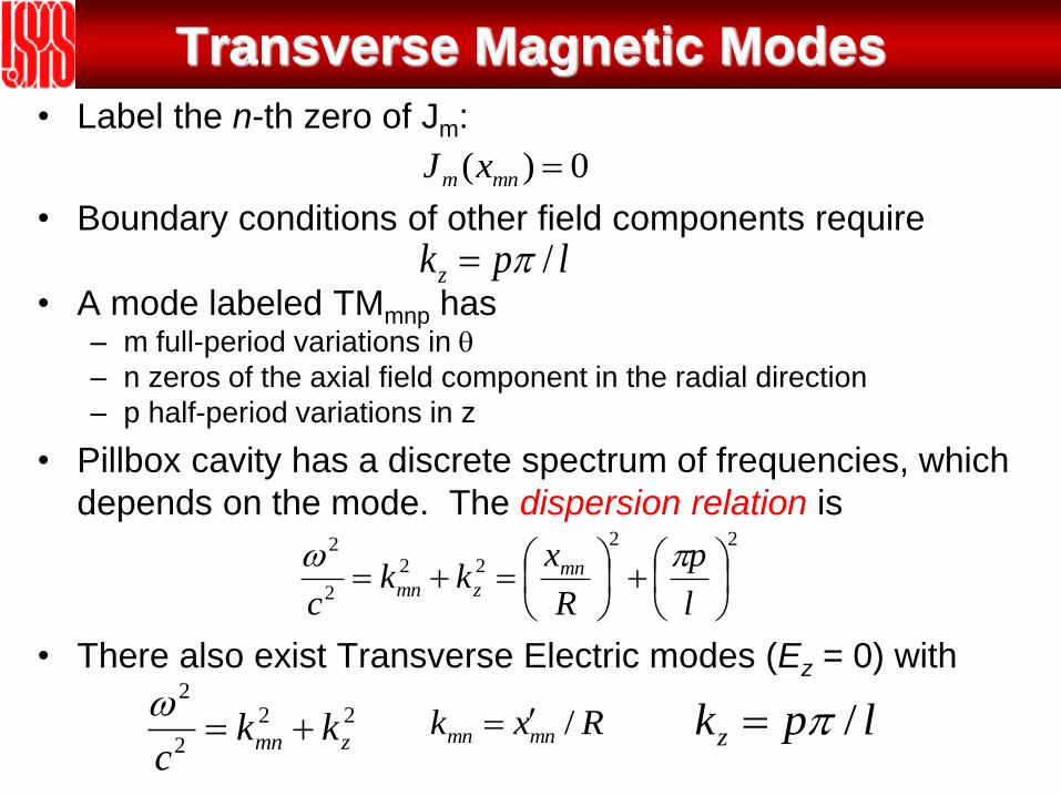
Transverse Magnetic Modes

• Label the n-th zero of Jm:

• Boundary conditions of other field components require

• A mode labeled TMmnp has – m full-period variations in

– n zeros of the axial field component in the radial direction

– p half-period variations in z

• Pillbox cavity has a discrete spectrum of frequencies, which

depends on the mode. The dispersion relation is

• There also exist Transverse Electric modes (Ez = 0) with

0)( mnm xJ

lpkz /

22

22

2

2

l

p

R

xkk

c

mnzmn

22

2

2

zmn kkc

Rxk mnmn / lpkz /

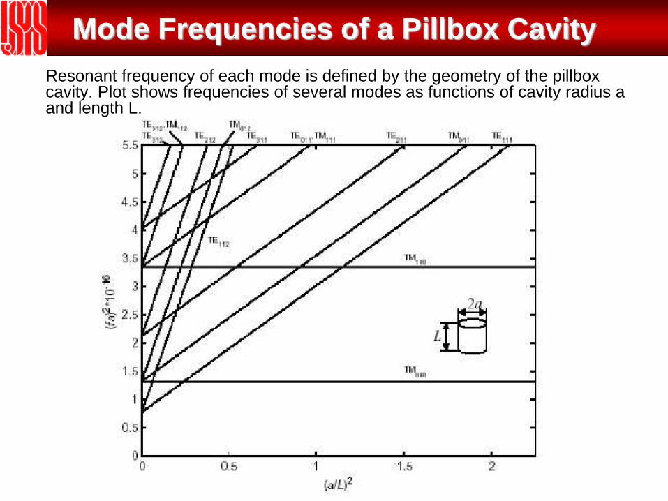
Mode Frequencies of a Pillbox Cavity

Resonant frequency of each mode is defined by the geometry of the pillbox cavity. Plot shows frequencies of several modes as functions of cavity radius a and length L.

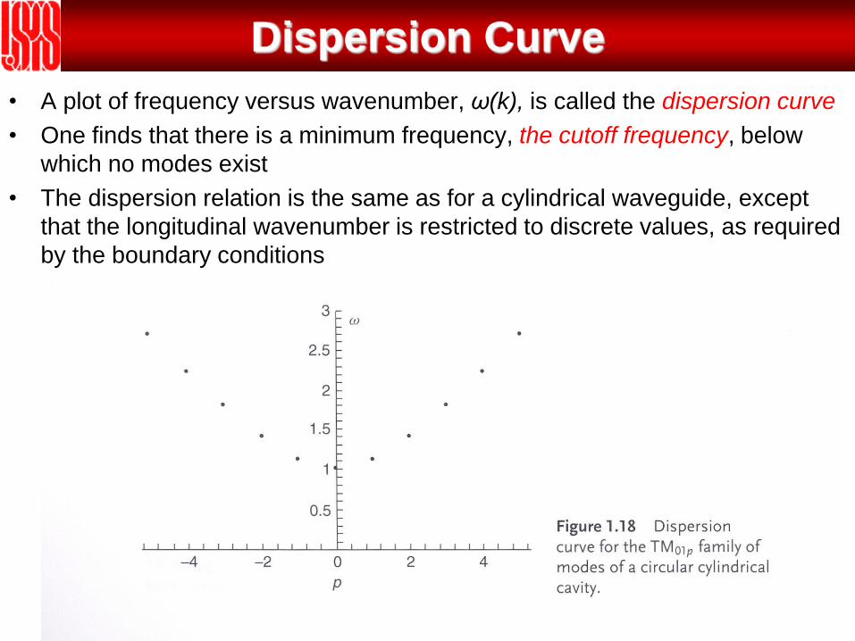
Dispersion Curve

• A plot of frequency versus wavenumber, ω(k), is called the dispersion curve

• One finds that there is a minimum frequency, the cutoff frequency, below

which no modes exist

• The dispersion relation is the same as for a cylindrical waveguide, except

that the longitudinal wavenumber is restricted to discrete values, as required

by the boundary conditions

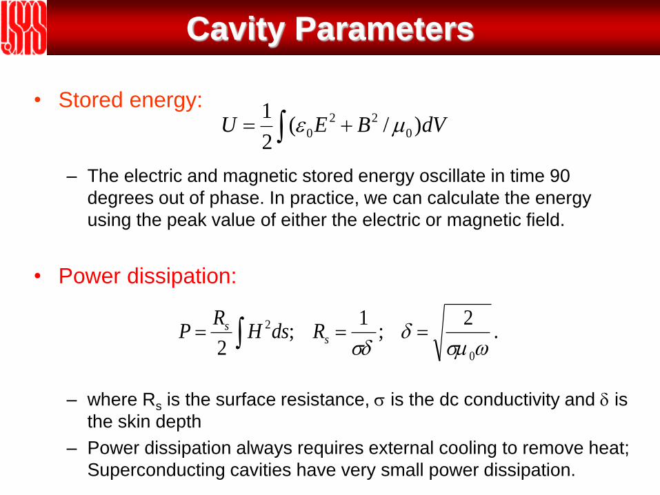
Cavity Parameters

• Stored energy:

– The electric and magnetic stored energy oscillate in time 90

degrees out of phase. In practice, we can calculate the energy

using the peak value of either the electric or magnetic field.

• Power dissipation:

– where Rs is the surface resistance, is the dc conductivity and is

the skin depth

– Power dissipation always requires external cooling to remove heat;

Superconducting cavities have very small power dissipation.

dVBEU )/(2

10

22

0

.2

;1

;2 0

2

s

s RdsHR

P

Cavity Parameters, cont’d

P

UQ

Q

UP

dt

dU

tQeUtU

)/(

00)(

Quality factor:

The quality factor is defined as 2π times the stored energy divided by the

energy dissipated per cycle

The quality factor is related to the damping of the electromagnetic

oscillation:

Rate of change of stored energy = - power dissipation

Since U is proportional to the square of the electric field:

)cos()( 0

)2/(

00

teEtEtQ

Thus, the electric field decays with a time constant, also called the filling

time 0/2 Q

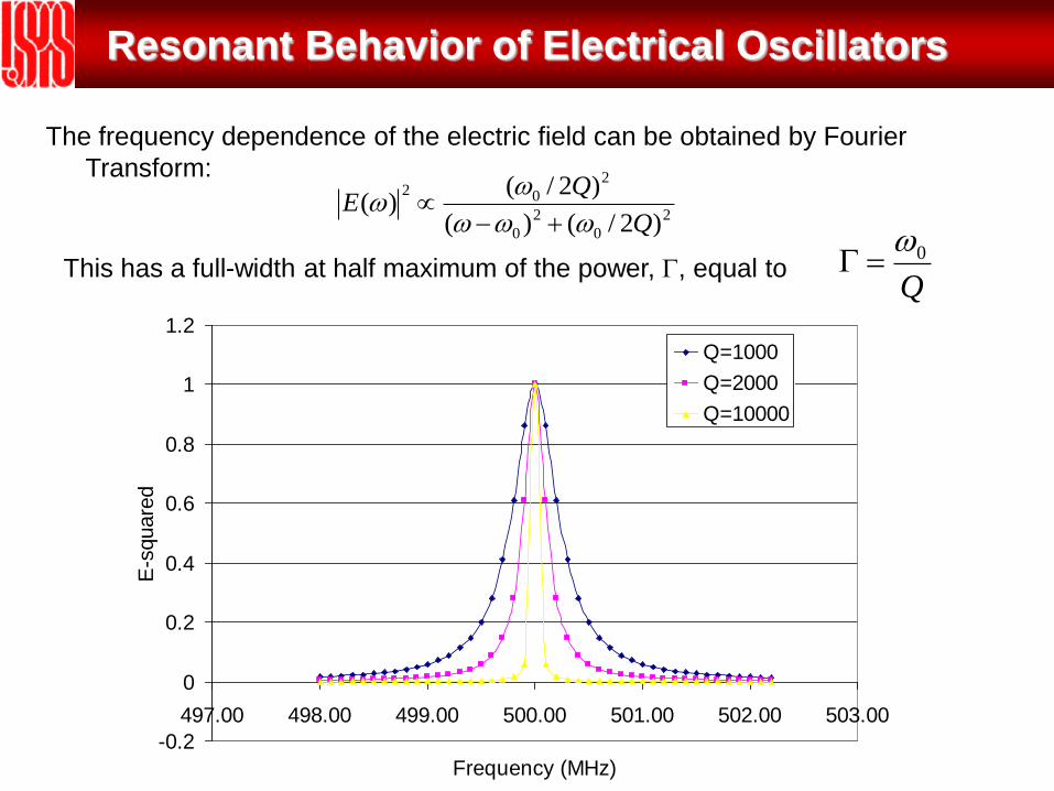
Resonant Behavior of Electrical Oscillators

-0.2

0

0.2

0.4

0.6

0.8

1

1.2

497.00 498.00 499.00 500.00 501.00 502.00 503.00

Frequency (MHz)

E-s

quare

d

Q=1000

Q=2000

Q=10000

The frequency dependence of the electric field can be obtained by Fourier

Transform:

2

0

2

0

2

02

)2/()(

)2/()(

Q

QE

This has a full-width at half maximum of the power, , equal to Q

0

The Pillbox Cavity Parameters

Stored energy:

Power dissipation:

Quality factor:

)405.2(2

2

1

2

0

2

0 JElRU

])[405.2(2

1

2

0

0

0 RlJERRP s

l

RR

c

P

UQ

s 1

405.2

2

0

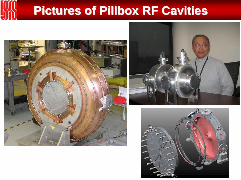
Pictures of Pillbox RF Cavities

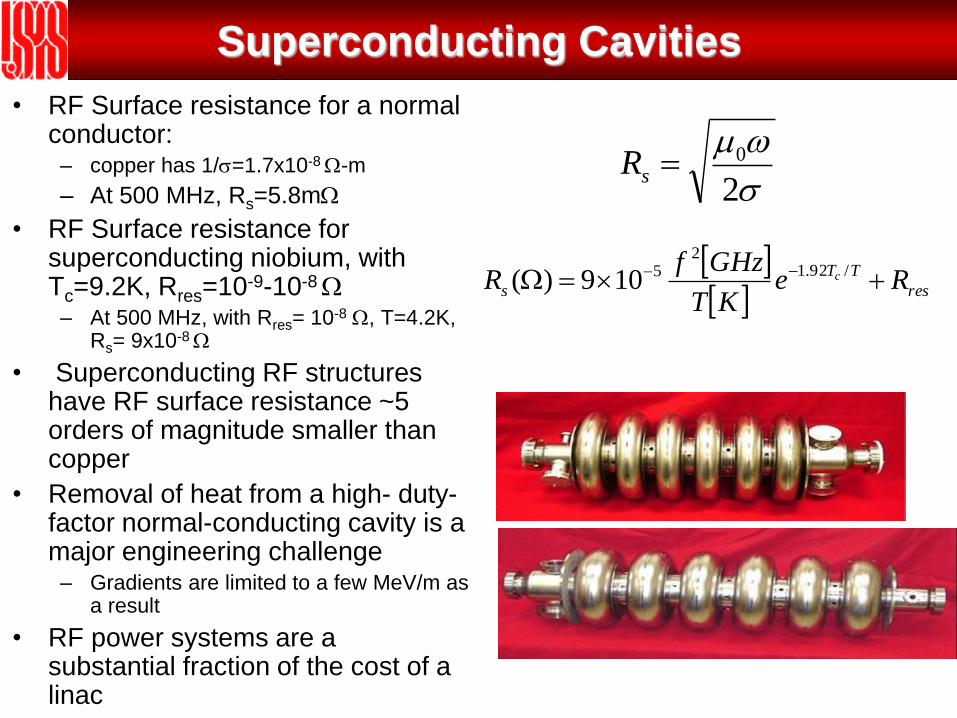
Superconducting Cavities

• RF Surface resistance for a normal conductor:

– copper has 1/=1.7x10-8 -m

– At 500 MHz, Rs=5.8m

• RF Surface resistance for superconducting niobium, with Tc=9.2K, Rres=10-9-10-8

– At 500 MHz, with Rres= 10-8 , T=4.2K, Rs= 9x10-8

• Superconducting RF structures have RF surface resistance ~5 orders of magnitude smaller than copper

• Removal of heat from a high- duty-factor normal-conducting cavity is a major engineering challenge

– Gradients are limited to a few MeV/m as a result

• RF power systems are a substantial fraction of the cost of a linac

2

0sR

res

TT

s ReKT

GHzfR c

/92.12

5109)(

Recap

• We found a solution to the wave equation with cylindrical boundary

conditions appropriate for a pillbox-cavity.

• This solution has two non-zero field components:

– Longitudinal Electric field (Yea! We can accelerate particles with

this.) that depends on radius, and

– Azimuthal magnetic field (Uh-oh….wait and see.) that depends

on radius.

• This cavity has a resonant frequency that depends on the

geometrical dimensions (radius only!).

• Because of finite conductivity, the cavity has a finite quality factor,

and therefore the cavity resonates over a narrow range of

frequencies, determined by Q.

• An infinite number of modes can be excited in a pillbox cavity; their

frequencies are determined by their mode numbers.

• The TM010 mode is the most commonly used mode for acceleration.

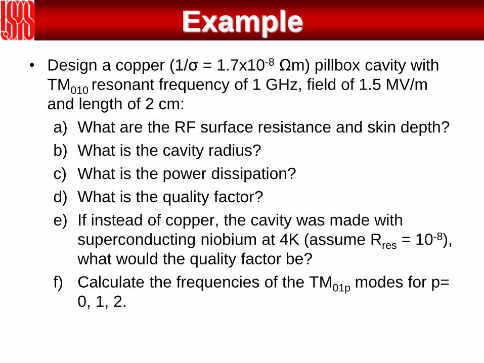
Example

• Design a copper (1/σ = 1.7x10-8 Ωm) pillbox cavity with

TM010 resonant frequency of 1 GHz, field of 1.5 MV/m

and length of 2 cm:

a) What are the RF surface resistance and skin depth?

b) What is the cavity radius?

c) What is the power dissipation?

d) What is the quality factor?

e) If instead of copper, the cavity was made with

superconducting niobium at 4K (assume Rres = 10-8),

what would the quality factor be?

f) Calculate the frequencies of the TM01p modes for p=

0, 1, 2.