Partial Regularity results for degenerate elliptic

systems

Bianca Stroffolini∗

Abstract

We present a partial Holder regularity result for solutions of degenerate systems

divA( · , Du) = 0 in Ω,

on bounded domains in the weak sense. Here certain continuity, monotonicity, growth and struc-ture condition are imposed on the coefficients, including an asymptotic Uhlenbeck behavior closeto the origin. Pursuing an approach of Duzaar and Mingione [17], we combine non-degenerateand degenerate harmonic-type approximation lemmas for the proof of the partial regularity result,giving several extensions and simplifications. In particular, we benefit from a direct proof of theapproximation lemma [11] that simplifies and unifies the proof in the power growth case. Moreover,we give the dimension reduction for the set of singular points.

MSC (2010): 35J45, 35J70

1 Introduction

In these notes I will present an approach towards regularity of weak solutions to possibly degenerateelliptic problems, that is mainly contained in the paper [3] for differential forms. We study weak solutionsu ∈W 1,p(Ω,RN ) with Ω a bounded domain in Rn, n,N ≥ 2, to nonlinear systems of the form

divA( · , Du) = 0 in Ω, (1.1)

where the coefficients are Holder continuous with respect to the first variable, with some exponentβ ∈ (0, 1), and of class C1 (possibly apart from the origin) with respect to the second variable with astandard p-growth condition. The main focus is set on the ellipticity condition: we allow a monotonicityor ellipticity condition which shows a degenerate (when p > 2) or singular (when p < 2) behavior in theorigin and which is usually expressed by the assumption

〈A(x, z)−A(x, z), z − z 〉 ≥ ν (µ2 + |z|2 + |z|2)p−22 |z − z|2

for all x ∈ Ω and all z, z ∈ RN for some µ ≥ 0. The nondegenerate situation refers to the case whereµ > 0 (and by changing the value ν these cases can be reduced to the model case µ = 1), whereas wehere treat the degenerate case µ = 0, meaning that we are dealing with a lack of ellipticity in the sensethat no uniform bound on the ellipticity constant is available for p 6= 2. We highlight that the quadraticcase does not impose any additional difficulties and is already covered by the standard regularity theory.

Let us first recall some of the well known facts for nondegenerate systems. In the vectorial caseN > 2 – in contrast to the scalar case N = 1 – we cannot in general expect that a weak solutionto the nonlinear elliptic system (1.1) is a classical solution (see e.g. the counterexamples in [6, 24]).Instead only a partial regularity result holds true, in the sense that we find an open subset Ω0 ⊂ Ω withLn(Ω \Ω0) = 0 such that Du is locally Holder continuous on Ω0 with optimal exponent β given by theexponent in the Holder continuity assumption on the x-dependency of the coefficients. These resultswere first obtained by Giusti and Miranda [23] via the indirect blow-up technique, then by Giaquinta,

∗B. Stroffolini, Dipartimento di Matematica e Applicazioni, Universita di Napoli Federico II, Via Cintia, 80126 Napoli,Italy. E-mail: bstroffo@unina.it Version: November 2, 2015

1

2 B. Stroffolini

Modica and Ivert [21, 27] via the direct method, and finally Duzaar and Grotowski [12] gave a new proofbased on the method of A-harmonic approximation introduced by Duzaar and Steffen [18]. For furtherreferences and in particular for related results concerning variational problems we refer to Mingione’ssurvey article [33].

In the degenerate case µ = 0 no (partial) regularity result seems to be known for such generalsystems. However, supposing some additional assumptions on the structure of the system, Uhlenbecksucceeded in her fundamental paper [37] in showing that Moser-type techniques may be applied andthat the classical regularity results of De Giorgi, Nash and Moser can be extended to systems of thisspecial form (often called Uhlenbeck structure). A prototype of these systems is the p-Laplace systemwith A(z) = |z|p−2z. More precisely, she stated in the superquadratic case (for systems without explicitdependency on the space variable) that the gradient of the solution is globally Holder continuous inthe interior with an exponent depending only on the space dimension n and the ellipticity ratio ν/L.We emphasize that Uhlenbeck’s proof was carried out in the more general setting of RN -valued closed`-differential forms ω ∈ Lp(Ω,Λ`Rn) solving the weak formulation to

d∗ρ(|ω|)ω = 0 in Ω ,

where ρ satisfies the Uhlenbeck structure assumptions (see p. 5). Further results concerning the regu-larity theory under such structure assumptions can for instance be found in [36, 22, 1, 20, 25, 29, 30, 10].We highlight that Hamburger [25] gave an extension of Uhlenbeck’s results in the setting of differentialforms on Riemannian manifolds with sufficiently smooth boundary. In particular, he used an elegantduality argument to derive the subquadratic result from the superquadratic one (see also [26]). Re-stricting ourselves to the special case of 1-forms it is clear that the regularity result also covers weaksolutions u ∈W 1,p(Ω,RN ).

Minimizers to variational integrals with possibly degenerately quasiconvex integrands were alreadyconsidered Duzaar and Mingione [14]. They observed that the non-degenerate and the degenerate theorycan be combined in the following way: as long as the gradient variable keeps away from the origin, thesystem is also for µ = 0 not singular/degenerate, and therefore a local partial regularity result holds truewithout an additional Uhlenbeck structure assumption. In contrast, if the origin is approached, then byrequiring this crucial structure assumption even full regularity is locally expected. In fact, this strategyof distinguishing the local type of ellipticity was applied successfully in [14] in case of an asymptoticbehavior like the p-Laplace system close to the origin, and as a final result minimizers were proved tobe locally of class C1,α for some α > 0 (specified in the neighborhood of points where Du does notvanish) outside a set of Lebesgue measure zero. In order to obtain an estimate for the decay of a suitableexcess quantity, we employ local comparison principles based on harmonic-type approximation lemmaswhich are inspired by Simon’s proof of the regularity theorem of Allard and which extend the method ofharmonic approximation (i. e. approximating with functions solving the Laplace equation) in a naturalway to bounded elliptic operators with constant coefficients or to even more general monotone operators.Here it is worth to remark that we give a direct proof of the harmonic approximation lemma, motivatedfrom [11], and as a consequence the whole proof of the main partial regularity result is direct and weobtain a good control of the regularity estimates in terms of the structure constants. The importantfeature of the comparison system resulting from this harmonic-type approximation is the availability ofgood a priori estimates for its weak solutions (more precisely, solutions to linear systems with constantcoefficients are known to be smooth, and solutions to Uhlenbeck systems are known to admit at leastHolder continuous gradients). In case of systems with degeneracy in the origin the above-mentioneddistinction of the two different situations is accomplished as follows: if the average of the gradient is nottoo small compared to the excess quantity, then we deal with the non-degenerate situation and the usualcomparison with the solution to the linearized system is performed via the A-harmonic approximationlemma (see Proposition 7.1). If in contrast the average of the gradient is very small (again compared tothe excess), then we are in the degenerate situation, meaning that the solution is approximately solvingan Uhlenbeck system, and it is therefore compared to the exact solution of this Uhlenbeck system (seeProposition 7.3). These two decay estimates are then matched together in an iteration scheme as in[14], ending up with the desired partial regularity result.

Partial Regularity results for degenerate elliptic systems 3

On the one hand, we give a generalization of the existing results concerning possibly degenerateproblems. We pursue an approach proposed by Duzaar and Mingione [17] in order to extend the knownresults dealing with a possible degeneracy at the origin like the p-Laplace system to more general onesthat may behave at the origin like any arbitrary system of Uhlenbeck structure; a similar generalizationwas also suggested by Schmidt [35] who obtained the corresponding partial regularity result for degen-erate variational functionals under (p, q)-growth conditions. This first aim is essentially achieved by theuse of an extension of the p-harmonic approximation lemma from [15] (and similar to the one in [11]),namely the a-harmonic approximation Lemma 4.3.

Once the partial regularity result is achieved, it is natural to ask whether the Hausdorff dimension ofthe singular set can still be improved. We first note that for degenerate Uhlenbeck systems the (interior)singular set is indeed empty – due to the special structure of the coefficients. Turning our attentionto the non-degenerate situation without any structure assumptions, much less is known. Indeed, inthe course of proving regularity of the gradient Du for classical solutions u ∈ W 1,p(Ω,RN ), the set ofregular points is characterized, which in turn yields as a first and immediate consequence of a measuredensity result that the singular set is of Lebesgue measure zero. An estimate of the Hausdorff dimensionwas firstly investigated in the case of differentiable systems by Campanato in the 80’s. The proof reliedon the possibility of differentiating the system and obtaining existence of second-order derivatives ofthe solution. The first one who built a bridge between Holder continuity of the coefficients and size ofthe singular set was Mingione [32, 31]: he showed that the singular set Ω \ Ω0 is not only negligiblewith respect to the Lebesgue measure, but that its Hausdorff dimension is actually not greater thann − 2β (with β the degree of Holder continuity of the coefficients). For related results on dimensionreduction of the singular set in the context of convex variational integrals we refer to [28]. By means ofthe machinery of fractional Sobolev spaces and the differentiability of the system in a fractional sensedeveloped in the previous papers, this upper bound on the Hausdorff dimension of the singular set isshown to be still valid for the solutions under consideration in this paper.

In conclusion, the main regularity result of our paper in the special case of classical weak solutioncan be stated as follows:

Theorem 1.1: Let Ω ⊂ Rn be a bounded domain, p ∈ (1,∞), and consider a weak solution u ∈W 1,p(Ω,RN ) to the system (1.1) under assumptions corresponding to (H1)–(H5) given in Section 2.Then there exists an open subset Ω0 ⊂ Ω such that

u ∈ C1,σloc (Ω0,RN ) and dimH

(Ω \ Ω0

)≤ n− 2β ,

where σ is an exponent depending only on n,N, p, L, ν and β.

2 Structure conditions and main results

We start with Ω a bounded domain in Rn and we suppose that u ∈ Lp(Ω,RN ), with 1 < p < ∞, is aweak solution to the elliptic system

divA( · , Du) = 0 in Ω, (2.1)

for a vector field A : Ω × RN → RN satisfying some structure conditions: the mapping P 7→ A(x,P)is of class C0(RN ,RN ) ∩ C1(RN \ 0,RN ), and for fixed numbers 0 < ν ≤ L, all x, x ∈ Ω and allP, P ∈ RN the following assumptions concerning growth, ellipticity and continuity hold true:

A is Lipschitz continuous with respect to P with(H1)

|A(x,P)−A(x, P)| ≤ L (|P|2 + |P|2)p−22 |P− P| ,

DPA is Holder continuous with some exponent α ∈ (0, |p− 2|) such that(H2)

|DPA(x,P)−DPA(x, P)| ≤ L (|P|2 + |P|2)p−2−α

2 |P− P|α

holds for p > 2, whereas in the subquadratic case p ∈ (1, 2) there holds for all P, P 6= 0

4 B. Stroffolini

|DPA(x,P)−DPA(x, P)| ≤ L |P|p−2|P|p−2(|P|2 + |P|2)2−p−α

2 |P− P|α,A is degenerately monotone:(H3)

〈A(x,P)−A(x, P),P− P 〉 ≥ ν (|P|2 + |P|2)p−22 |P− P|2 ,

A is Holder continuous with respect to its first argument with exponent β ∈ (0, 1):(H4)

|A(x,P)−A(x,P)| ≤ L |P|p−1 |x− x|β ,A is of Uhlenbeck structure at 0, i. e. there exists a non-decreasing function(H5)

µ : R+ → R+ such that for all P ∈ RN with |P| ≤ µ(t) there holds

|A(x, P)− ρx(|P|) P| ≤ t |P|p−1

uniformly for all x ∈ Ω, where ρx is a family of functions satisfying (G1)–(G3)introduced on p. 5 further below.

We first note that – due to the growth condition (H1), the monotonicity in (H3) and the Uhlenbecktype behavior at 0 in (H5) – the coefficients A(x,P) exhibit a polynomial growth with respect to thevariable P, namely for all x ∈ Ω, P ∈ RN there holds

ν |P|p−1 ≤ |A(x,P)| ≤ L |P|p−1 . (2.2)

Secondly, in view of the differentiability of P 7→ A(x, z), we remark that (H1) and (H3) imply a growthand (degenerate) ellipticity condition for DPA(x,P), more precisely, we have

|DPA(x,P)| ≤ L |P|p−2 , (2.3)

〈DPA(x,P) ξ, ξ 〉 ≥ ν |P|p−2 |ξ|2 (2.4)

for all ξ ∈ RN , every x ∈ Ω and all P ∈ RN \ 0 (for p > 2 these inequalities are also valid for P = 0).

Example: A simple example or model case for the systems under consideration in this paper are thefollowing type of x-depending versions of the p-Laplace system:

A(x,P) := β(x) |P|p−2 P

for all P ∈ RN and with β(·) a continuous function in Ω taking values in [ν, L] with Holder exponent β.

For a field P ∈ Lp(Br(x0),RN ) we now introduce the excess

Φ(P;x0, r,P0) :=

∫−Br(x0)

|V|P0|(P−P0)|2 for every P0 ∈ RN ,

where Vµ(ξ) := (µ2 + |ξ|2)(p−2)/4ξ. In the sequel this excess shall frequently be used for the choiceP0 = (P)x0,ρ, where (P)x0,r =

∫−Br(x0)

P is an abbreviation for the meanvalue of P on the ball Br(x0).

As mentioned in [35] , [11] this excess is equivalent to∫−Br(x0)

|V0(P)− V0(P0)|2 (2.5)

up to a constant depending only on n,N, p , and also to the one used in [14] . With this notation athand we can now state our main regularity result for weak solutions to (2.1) on a bounded domain inRn:

Theorem 2.1: Let Ω ⊂ Rn be a bounded domain, p ∈ (1,∞) and consider a weak solution u ∈W 1,p(Ω,RN ) to the homogeneous system (2.1) under the assumptions (H1)–(H5). Then there existsσ = σ(n,N, p, L, ν, β) and an open subset Ω0 ⊂ Ω such that

∇u ∈ C0,σloc (Ω0(∇u),RN ) and |Ω \ Ω0| = 0

Partial Regularity results for degenerate elliptic systems 5

with the following characterization of the set of regular points:

Ω0 = R :=x0 ∈ Ω: : lim inf

r0Φ(x0, r, (∇u)x0,r) = 0 and lim sup

r0

∣∣(∇u)x0,r

∣∣ < ∞ .Moreover, if x0 ∈ Ω0(∇u) and

lim supr0

∣∣(∇u)x0,r

∣∣pΦ(x0, r, (∇u)x0,r)

= ∞ , (2.6)

then ∇u is locally Holder continuous with exponent minβ, 2β/p. Furthermore, if ∇u(x0) 6= 0, then∇u ∈ C0,β(Bs(x0),RN ) for some s > 0.

Remark: More precisely, in points x0 where (2.6) is not satisfied, the local Holder continuity on theregular set Ω0 is determined by the exponent from the Holder continuity of the coefficients with respectto the first variable and the asymptotic degenerate system in the origin in a neighborhood of x0,namely the exponent σ is given by minγ, β in the subquadratic case and by min2γ/p, 2β/p in thesuperquadratic case. Here γ ∈ (0, 1) is the number from the a priori estimate for weak solutions tosystems of Uhlenbeck-type given in Proposition 3.1 below (we note that γ does not depend on the pointx0 since the parameters n,N, p, L and ν remain fixed for all functions ρx).

As a second result we give the dimension reduction for the singular set, which states a relationbetween the degree of regularity of the coefficients and the size of the Hausdorff dimension of thesingular set:

Theorem 2.2: Let Ω ⊂ Rn be a bounded domain, p ∈ (1,∞) and consider a weak solution ∇u ∈Lp(Ω,RN ) to the system (2.1) under the assumptions (H1)–(H5). Then we have

dimH

(Ω \ Ω0(∇u)

)≤ n− 2β .

3 Uhlenbeck result

A regularity result for degenerate Uhlenbeck systems. I will state a comparison estimate for specialnonlinear degenerate systems which exhibit a particular structure that allows to prove everywhereregularity of the solution. More precisely, we consider vector fields of the form

a(P) = ρ(|P|) P

for every P ∈ RnN . For the function ρ : [0,∞) → [0,∞) we shall assume the following continuity,ellipticity and growth conditions:

The function t 7→ ρ(t) is of class C0([0,∞]) ∩ C1((0,∞]) ,(G1)

There hold the inequalities(G2)

ν tp−2 ≤ ρ(t) ≤ L tp−2

and

ν tp−2 ≤ ρ(t) + ρ′(t) t ≤ L tp−2 ,

There exists a Holder exponent βρ ∈ (0,min1, |p− 2|) such that(G3)

|ρ′(s) s− ρ′(t) t| ≤ L (|s|2 + |t|2)p−2−βρ

2 |s− t|βρ .

for all s, t ∈ (0,∞), and some p ≥ 2, 0 < ν ≤ L. The model case of a vector field satisfying theseconditions is the p-Laplace system, i. e. the vector field give by a(P) = |P|p−2P for all P ∈ RnN . Forsystems satisfying the above Uhlenbeck structure assumptions the following regularity result can beretrieved from [37, Theorem 3.2], [30]) and [25, Theorem 4.1]:

6 B. Stroffolini

Proposition 3.1: Let p ∈ (1,∞). There exists a constant c ≥ 1 and an exponent γ ∈ (0, 1) dependingonly on n,N, p, L and ν such that the following statement holds true: whenever h ∈W 1,p(BR(x0),RN )is a weak solution of the system

div(ρ(|∇h|)∇h

)= 0 in BR(x0) ,

where ρ(·) fullfills the assumptions (G1)–(G3), then for every 0 < r < R there hold

supBR/2(x0)

|∇h|p ≤ c

∫−BR(x0)

|∇h|p and Φ(x0, r, (∇h)x0,r) ≤ c( rR

)2γ

Φ(x0, R, (∇h)x0,R) .

4 Harmonic approximation lemmas

In this section we shall state two harmonic-type approximation lemmas which are adapted to thedegenerate and the non-degenerate situation and which will allow us to compare the solution to theoriginal system to the solution of an easier systems (for which good a priori estimates are available).To this aim we first need a result on Lipschitz-truncation, which from its original formulation can berestated as follows:

Proposition 4.1 (Lipschitz truncation, cf. [19], Prop. 4.1): Let B ⊂ Rn be a ball. There existsa constant c depending only on n,N, p and B such that whenever χk 0 weakly in W 1,p

T (B,RN ), then

for every λ > 0 there exists a sequence χλkk∈N of maps χλk ∈W1,∞T (B,RN ) such that

‖χλk‖W 1,∞ ≤ c λ .

Moreover, up to a set of Lebesgue measure zero we have

z ∈ B : χλk(z) 6= χk(z) ⊂ z ∈ B : M(∇χk)(z) > λ ,

where M denotes the maximal operator restricted to B.

Due to the direct approach for the proof of Lemma 4.3 we in fact need it only in a simpler version,namely for single functions instead of weakly converging sequences. However, there are much moreinvolved Lipschitz truncation lemmas available in the literature, such as on general domains, versionsinvolving sequences of truncations and variable exponent in [9, Theorem 2.5, Theorem 4.4]), versionstruncating at two different levels (one for the function itself, the second one as above for its gradient) etc.In this paper we shall use a consequence of the previous truncation Lemma 4.1 from [11] for a version

concerning the existence of a good truncation level in the setting of Sobolev-Orlicz spaces W 1,φT (B,Λ`).

I will state it in the case of power functions.

Corollary 4.2 ([11]): For every ε > 0 there exists c > 0 depending only on n,N, p such that thefollowing statement holds: If B ⊂ Rn is a ball and χ ∈ W 1,p

0 (B,Λ`), then for every m0 ∈ N and γ > 0there exists λ ∈ [γ, 2m0γ] such that the Lipschitz truncation χλ ∈W 1,∞

T (B,RN ) of Theorem 4.1 satisfies

‖∇χλ‖∞ ≤ c λ ,∫−B

|∇χλ|p 1χλ 6=χ dx ≤ c

∫−B

λp 1χλ 6=χ dx ≤c

m0

∫−B

|∇χ|p dx .

Restricting ourselves to the case of power growth in order to keep the setting as simple as possible, wenow derive by similar techniques a suitable version which will apply not only to the p-Laplace system, butalso to more general monotone operators. In what follows we consider vector fields a : Ω × RN → RNwhich are measurable with respect to the first variable, continuous in the second, and which satisfygrowth and monotonicity conditions of the form

∣∣a(x,P)∣∣ ≤ L

(µ2 + |P|2

) p−12 ,

a(x,P) ·P ≥ ν(µ2 + |P|2

) p−22 |P|2 ,(

a(x,P)− a(x, P))· (P− P) ≥ ν

(µ2 + |P|2 + |P|2

) p−22 |P− P|2

(4.1)

Partial Regularity results for degenerate elliptic systems 7

for all x ∈ Ω, P, P ∈ RN , p > 1, µ ∈ [0, 1] and 0 < ν ≤ L. Furthermore, we assume that a(·, ·) isuniformly continuous on bounded subsets, i. e. that

|a(x,P)− a(x, P)| ≤ K(|P|+ |P|)ϑ(|P− P|) (4.2)

whenever x ∈ Ω, P, P ∈ RN , where K : [0,∞) → [0,∞) is a locally bounded, nondecreasing functionand ϑ : [0,∞)→ [0, 1] is a nondecreasing function with limt0 ϑ(t) = 0. We note that these assumptionsare in particular satisfied with µ = 0 for vector fields a(P) := ρ(|P|) P where ρ fullfills conditions (G1)and (G2) from the previous section. Following the notation of [7], we define for a convex functionφ ∈ C1((0,∞)) and µ ≥ 0 the shifted function φµ by

φµ(t) :=

∫ t

0

φ′µ(s) ds with φ′µ(t) :=φ′(µ+ t)

µ+ tt

for t > 0. In the case of powers φ(t) := tp, the excess function Vµ(t) introduced in Section 3 is equivalentto the shifted function (φµ(t))1/2 (up to a constant depending only on p) and relates to the operatora(·, ·) satisfying the assumption (4.1) above via the inequalities:

|a(x,P)| ≤ c(p, L)φ′µ(|P|) ,a(x,P) ·P ≥ ν |Vµ(P)|2 ≥ c−1(p) ν φµ(|P|) ,(a(x,P)− a(x, P)

)· (P− P) ≥ c−1(p) ν |Vµ(P)− Vµ(P)|2 .

(4.3)

We may now introduce the notion of an a-harmonic field: a field u ∈ W 1,p(Ω,RN ) is called a-harmonic in a domain Ω if a(·, ·) fulfills the growth assumption (4.1)1 and if∫

Ω

〈 a(x,∇u),∇η 〉 = 0 for every η ∈ C∞0 (Ω,RN ) .

Lemma 4.3 (a-harmonic approximation; cf. [11]): Let p ∈ (1,∞) and φ(t) = tp for all t ≥ 0. Forevery ε > 0 and every θ ∈ (0, 1) there exists δ > 0 which depends only on n,N, p, ν, L, θ and ε such thatthe following statement holds true: Let B ⊂ Rn be a ball. Whenever a(·, ·) : B × RN → RN is a vectorfield satisfying (4.1) and (4.2) and whenever χ ∈ W 1,p(B,RN ) is a vector field that is approximatelya-harmonic in the sense that∣∣∣ ∫−

B

〈 a(x,∇χ),∇η 〉∣∣∣ ≤ δ

(∫−B

φµ(|∇χ|) + φµ(‖∇η‖∞))

(4.4)

holds for all η ∈ C10 (B,RN ), then the unique a-harmonic h ∈W 1,p(B,RN ), h = χ on ∂B satisfies∫

−B

φµ(|∇h|) ≤ c(p, ν, L)

∫−B

φµ(|∇χ| and(∫−B

|Vµ(∇χ)− Vµ(∇h)|2θ) 1θ ≤ ε

∫−B

φµ(|∇χ|) .

Secondly, we state a suitable version of the A-harmonic approximation lemma for both the super-and the subquadratic case. This version is proved by adjusting the proof of [18, Lemma 3.3], [13, Lemma6] and [34, Lemma 6.8], respectively, or in a similar way as in the proof of the a-harmonic approximationlemma presented above.

Lemma 4.4 (A-harmonic approximation): Let ν ≤ L be positive constants, p ∈ (1,∞) . Thenfor every ε > 0 there exists a positive number δ ∈ (0, 1] depending only on n,N, p, νL and ε with thefollowing property: whenever A is a bilinear form on RnN which is elliptic in the sense of Legendre-Hadamard with ellipticity constant ν and upper bound L and whenever χ ∈ W 1,p(Br,RN ) satisfying∫−Br|V1(∇χ)|2 ≤ ς2 ≤ 1 is approximately A-harmonic in the sense that∣∣∣ ∫−

Br

A(∇χ,∇η) dx∣∣∣ ≤ ς δ sup

Br

|∇η| (4.5)

8 B. Stroffolini

holds for all η ∈ C10 (Br,RN ), then there exists an A-harmonic map h ∈ W 1,p(Br,RN ), h = χ on ∂Br,

which satisfies

supBr/2

|∇h|+ r supBr/2

|D2h| ≤ c and

∫−Br/2

∣∣∣V1

(χ− ςhr

)∣∣∣2 dx ≤ ς2 ε .

for a constant c depending only on n,N, p, ν and L.

5 A Caccioppoli inequality

As usual the first step in proving a regularity theorem for solutions of elliptic systems is to establisha suitable reverse-Poincare or Caccioppoli-type inequality. This version of the Caccioppoli inequalitytakes into account the possible degeneracy of the monotonicity condition (H3) (and therefore also of theellipticity condition).

Lemma 5.1: Let p ∈ (1,∞) and consider a weak solution u ∈W 1,p(Br(x0),RN ), r < 1, to the system(2.1) under the assumptions (H1), (H3) and (H4). Then, for ξ ∈ Lp(Br(x0),RN ) and ζ ∈ RnN thereholds ∫

−Br/2(x0)

∣∣V|ζ|(∇u− ζ)∣∣2 ≤ c

∫−Br(x0)

∣∣∣V|ζ|(u− ξ − ζ · (x− x0)

r

)∣∣∣2 + c |ζ|p r2β (5.1)

for a constant c depending only on p, L and ν.

Proof: Without loss of generality we may assume x0 = 0. We consider a cut-off function η ∈C∞0 (Br, [0, 1]) such that η ≡ 1 on Br/2 and |Dη| ≤ c

r . We may take ηp(u − ξ − ζ · x) as a testfunction in (2.1). Using the assumptions and keeping in mind the properties of the cut-off function η,we thus arrive at the desired inequality.

Remark 5.2: Applying the Poincare inquality we get immediately a reverse Holder’ s inequality for∇u− ζ for a θ < 1∫

−Br/2(x0)

∣∣V|ζ|(∇u− ζ)∣∣2 ≤ c

(∫−Br(x0)

∣∣V|ζ|(∇u− ζ)∣∣2θ) 1

θ

+ c |ζ|p r2β (5.2)

This would get a higher integrability result for ∇u− ζ.

6 Approximate A- and a-harmonicity

Our next aim is to find a framework in which the A-harmonic and the a-harmonic approximation lemma,respectively, can be applied. This means that we have to identify systems for which the smallnessconditions in the sense of (4.5) and (4.4) hold true (provided that additional smallness assumptions aresatisfied). This shall be accomplished in the non-degenerate case by linearization of the coefficients,whereas in the degenerate case assumption (H5) allows to define a suitable Uhlenbeck-type system.

To start with the non-degenerate case we first recall the definition of the excess: for every ballBr(x0) ⊂ Rn, a fixed function u ∈ W 1,p(Br(x0),RN ), p ∈ (1,∞), and every P0 ∈ RnN the excess of uis defined via

Φ(x0, r,P0) :=

∫−Br(x0)

∣∣V|P0|(∇u−P0)∣∣2 .

Lemma 6.1 (Approximate A-harmonicity): Let p ∈ (1,∞). There exists a constant cA dependingonly on p and L such that for every weak solution u ∈W 1,p(Br(x0),RN ), r < 1, to system (2.1) underthe assumptions (H2) and (H4), and every P0 ∈ RnN such that |P0| 6= 0 6= Φ(x0, r,P0) we have∣∣∣ ∫−Br(x0)

〈DPA(x0,P0) |P0|1−p (∇u−P0),∇η 〉∣∣∣ ≤ cA

[( Φ(r)

|P0|p) 1

2 +|p−2|

2p

+( Φ(r)

|P0|p) 1

2 +α2

+rβ]

supBr(x0)

|∇η|

for all η ∈ C10 (Br(x0),RN ). Here we have abbreviated Φ(x0, r,P0) by Φ(r).

Partial Regularity results for degenerate elliptic systems 9

To treat the degenerate case where the system under consideration is close to a possibly degeneratesystem of Uhlenbeck structure, we define analogously to [14]

Ψ(x0, r) =

∫−Br(x0)

|∇u|p .

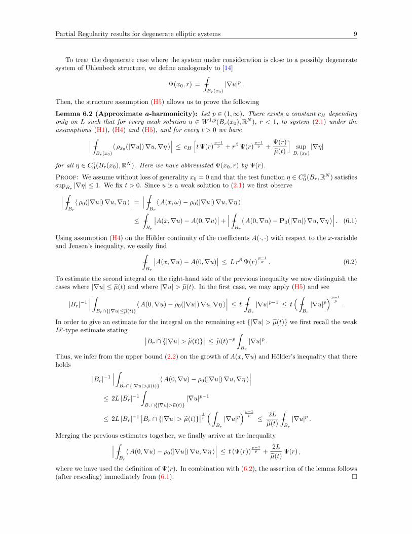
Then, the structure assumption (H5) allows us to prove the following

Lemma 6.2 (Approximate a-harmonicity): Let p ∈ (1,∞). There exists a constant cH dependingonly on L such that for every weak solution u ∈ W 1,p(Br(x0),RN ), r < 1, to system (2.1) under theassumptions (H1), (H4) and (H5), and for every t > 0 we have∣∣∣ ∫−

Br(x0)

〈 ρx0(|∇u|)∇u,∇η 〉∣∣∣ ≤ cH

[tΨ(r)

p−1p + rβ Ψ(r)

p−1p +

Ψ(r)

µ(t)

]supBr(x0)

|∇η|

for all η ∈ C10 (Br(x0),RN ). Here we have abbreviated Ψ(x0, r) by Ψ(r).

Proof: We assume without loss of generality x0 = 0 and that the test function η ∈ C10 (Br,RN ) satisfies

supBr |∇η| ≤ 1. We fix t > 0. Since u is a weak solution to (2.1) we first observe∣∣∣ ∫−Br

〈 ρ0(|∇u|)∇u,∇η 〉∣∣∣ =

∣∣∣ ∫−Br

〈A(x, ω)− ρ0(|∇u|)∇u,∇η 〉∣∣∣

≤∫−Br

∣∣A(x,∇u)−A(0,∇u)∣∣+∣∣∣ ∫−Br

〈A(0,∇u)−P0(|∇u|)∇u,∇η 〉∣∣∣ . (6.1)

Using assumption (H4) on the Holder continuity of the coefficients A(·, ·) with respect to the x-variableand Jensen’s inequality, we easily find∫

−Br

∣∣A(x,∇u)−A(0,∇u)∣∣ ≤ Lrβ Ψ(r)

p−1p . (6.2)

To estimate the second integral on the right-hand side of the previous inequality we now distinguish thecases where |∇u| ≤ µ(t) and where |∇u| > µ(t). In the first case, we may apply (H5) and see

|Br|−1∣∣∣ ∫Br∩|∇u|≤µ(t)

〈A(0,∇u)− ρ0(|∇u|)∇u,∇η 〉∣∣∣ ≤ t

∫−Br

|∇u|p−1 ≤ t(∫−Br

|∇u|p) p−1

p

.

In order to give an estimate for the integral on the remaining set |∇u| > µ(t) we first recall the weakLp-type estimate stating ∣∣Br ∩ |∇u| > µ(t)

∣∣ ≤ µ(t)−p∫Br

|∇u|p .

Thus, we infer from the upper bound (2.2) on the growth of A(x,∇u) and Holder’s inequality that thereholds

|Br|−1∣∣∣ ∫Br∩|∇u|>µ(t)

〈A(0,∇u)− ρ0(|∇u|)∇u,∇η 〉∣∣∣

≤ 2L |Br|−1

∫Br∩|∇u|>µ(t)

|∇u|p−1

≤ 2L |Br|−1∣∣Br ∩ |∇u| > µ(t)

∣∣ 1p (∫Br

|∇u|p) p−1

p ≤ 2L

µ(t)

∫−Br

|∇u|p .

Merging the previous estimates together, we finally arrive at the inequality∣∣∣ ∫−Br

〈A(0,∇u)− ρ0(|∇u|)∇u,∇η 〉∣∣∣ ≤ t (Ψ(r))

p−1p +

2L

µ(t)Ψ(r) ,

where we have used the definition of Ψ(r). In combination with (6.2), the assertion of the lemma follows(after rescaling) immediately from (6.1).

10 B. Stroffolini

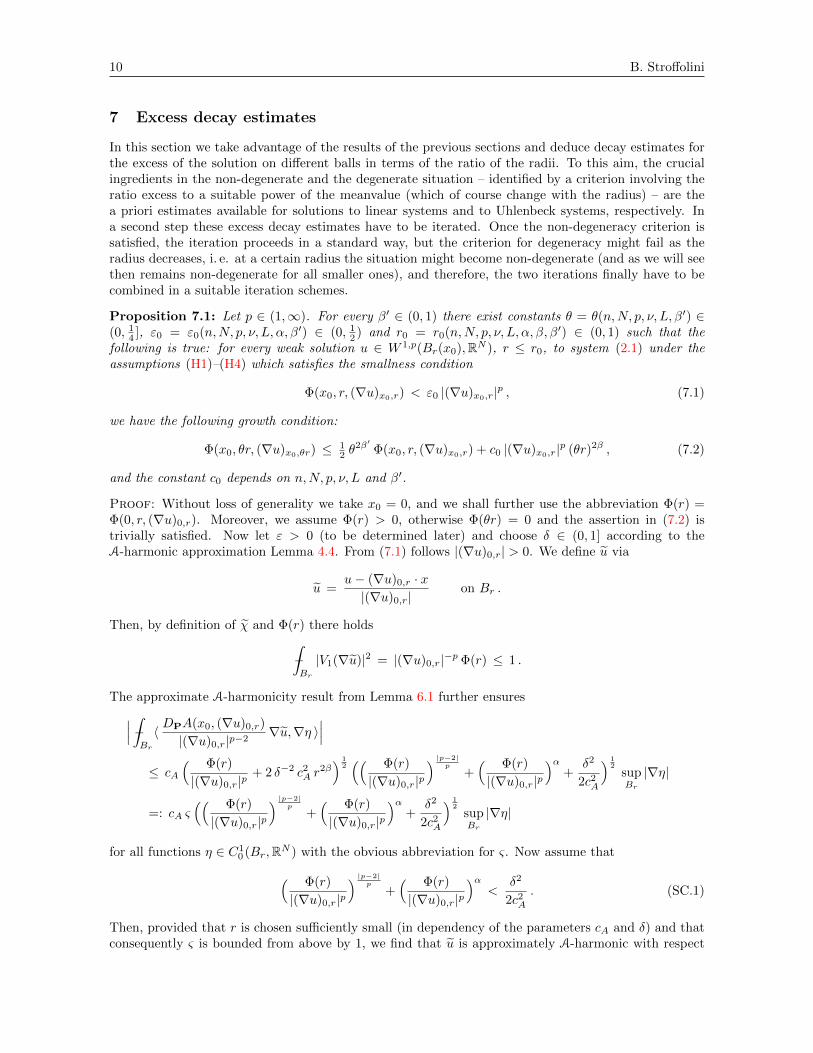
7 Excess decay estimates

In this section we take advantage of the results of the previous sections and deduce decay estimates forthe excess of the solution on different balls in terms of the ratio of the radii. To this aim, the crucialingredients in the non-degenerate and the degenerate situation – identified by a criterion involving theratio excess to a suitable power of the meanvalue (which of course change with the radius) – are thea priori estimates available for solutions to linear systems and to Uhlenbeck systems, respectively. Ina second step these excess decay estimates have to be iterated. Once the non-degeneracy criterion issatisfied, the iteration proceeds in a standard way, but the criterion for degeneracy might fail as theradius decreases, i. e. at a certain radius the situation might become non-degenerate (and as we will seethen remains non-degenerate for all smaller ones), and therefore, the two iterations finally have to becombined in a suitable iteration schemes.

Proposition 7.1: Let p ∈ (1,∞). For every β′ ∈ (0, 1) there exist constants θ = θ(n,N, p, ν, L, β′) ∈(0, 1

4 ], ε0 = ε0(n,N, p, ν, L, α, β′) ∈ (0, 12 ) and r0 = r0(n,N, p, ν, L, α, β, β′) ∈ (0, 1) such that the

following is true: for every weak solution u ∈ W 1,p(Br(x0),RN ), r ≤ r0, to system (2.1) under theassumptions (H1)–(H4) which satisfies the smallness condition

Φ(x0, r, (∇u)x0,r) < ε0 |(∇u)x0,r|p , (7.1)

we have the following growth condition:

Φ(x0, θr, (∇u)x0,θr) ≤ 12 θ

2β′ Φ(x0, r, (∇u)x0,r) + c0 |(∇u)x0,r|p (θr)2β , (7.2)

and the constant c0 depends on n,N, p, ν, L and β′.

Proof: Without loss of generality we take x0 = 0, and we shall further use the abbreviation Φ(r) =Φ(0, r, (∇u)0,r). Moreover, we assume Φ(r) > 0, otherwise Φ(θr) = 0 and the assertion in (7.2) istrivially satisfied. Now let ε > 0 (to be determined later) and choose δ ∈ (0, 1] according to theA-harmonic approximation Lemma 4.4. From (7.1) follows |(∇u)0,r| > 0. We define u via

u =u− (∇u)0,r · x|(∇u)0,r|

on Br .

Then, by definition of χ and Φ(r) there holds∫−Br

|V1(∇u)|2 = |(∇u)0,r|−p Φ(r) ≤ 1 .

The approximate A-harmonicity result from Lemma 6.1 further ensures∣∣∣ ∫−Br

〈 DPA(x0, (∇u)0,r)

|(∇u)0,r|p−2∇u,∇η 〉

∣∣∣≤ cA

( Φ(r)

|(∇u)0,r|p+ 2 δ−2 c2A r

2β) 1

2(( Φ(r)

|(∇u)0,r|p) |p−2|

p

+( Φ(r)

|(∇u)0,r|p)α

+δ2

2c2A

) 12

supBr

|∇η|

=: cA ς(( Φ(r)

|(∇u)0,r|p) |p−2|

p

+( Φ(r)

|(∇u)0,r|p)α

+δ2

2c2A

) 12

supBr

|∇η|

for all functions η ∈ C10 (Br,RN ) with the obvious abbreviation for ς. Now assume that( Φ(r)

|(∇u)0,r|p) |p−2|

p

+( Φ(r)

|(∇u)0,r|p)α

<δ2

2c2A. (SC.1)

Then, provided that r is chosen sufficiently small (in dependency of the parameters cA and δ) and thatconsequently ς is bounded from above by 1, we find that u is approximately A-harmonic with respect

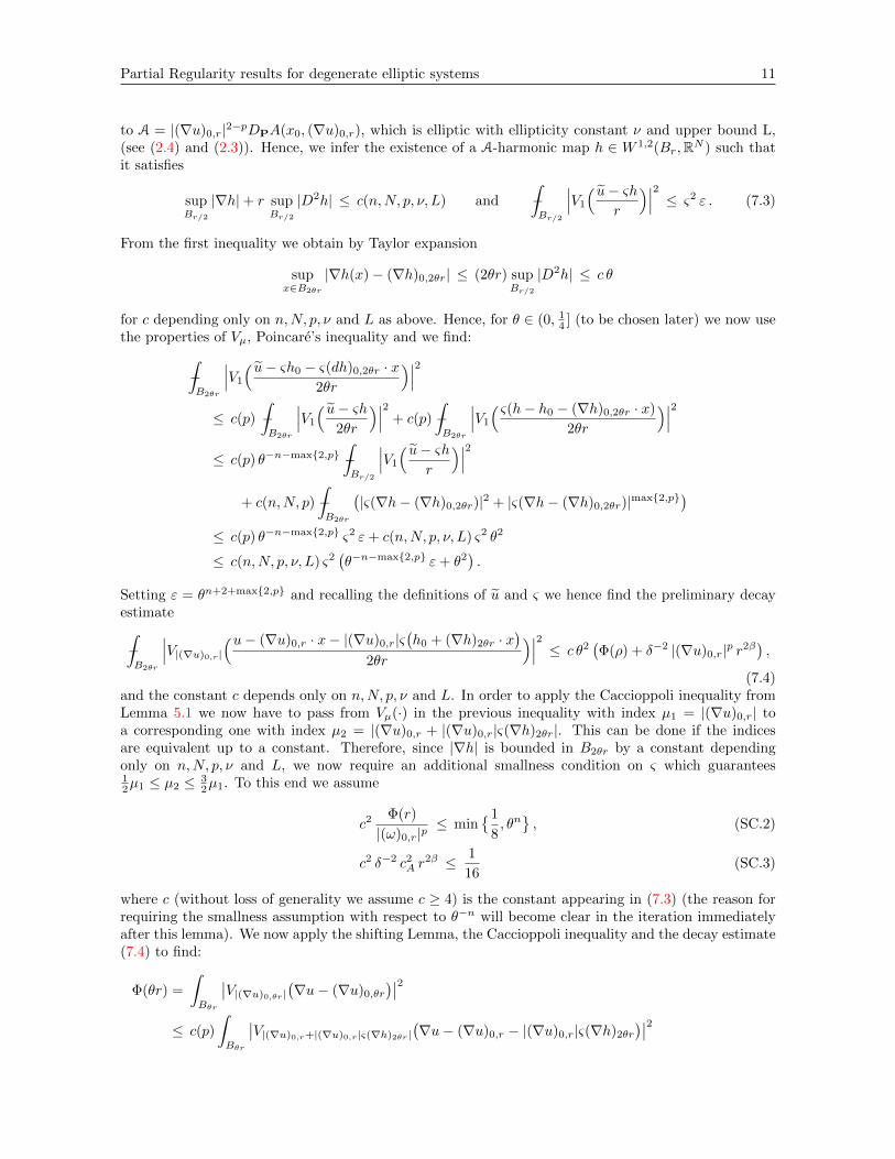
Partial Regularity results for degenerate elliptic systems 11

to A = |(∇u)0,r|2−pDPA(x0, (∇u)0,r), which is elliptic with ellipticity constant ν and upper bound L,(see (2.4) and (2.3)). Hence, we infer the existence of a A-harmonic map h ∈ W 1,2(Br,RN ) such thatit satisfies

supBr/2

|∇h|+ r supBr/2

|D2h| ≤ c(n,N, p, ν, L) and

∫−Br/2

∣∣∣V1

( u− ςhr

)∣∣∣2 ≤ ς2 ε . (7.3)

From the first inequality we obtain by Taylor expansion

supx∈B2θr

|∇h(x)− (∇h)0,2θr| ≤ (2θr) supBr/2

|D2h| ≤ c θ

for c depending only on n,N, p, ν and L as above. Hence, for θ ∈ (0, 14 ] (to be chosen later) we now use

the properties of Vµ, Poincare’s inequality and we find:∫−B2θr

∣∣∣V1

( u− ςh0 − ς(dh)0,2θr · x2θr

)∣∣∣2≤ c(p)

∫−B2θr

∣∣∣V1

( u− ςh2θr

)∣∣∣2 + c(p)

∫−B2θr

∣∣∣V1

( ς(h− h0 − (∇h)0,2θr · x)

2θr

)∣∣∣2≤ c(p) θ−n−max2,p

∫−Br/2

∣∣∣V1

( u− ςhr

)∣∣∣2+ c(n,N, p)

∫−B2θr

(|ς(∇h− (∇h)0,2θr)|2 + |ς(∇h− (∇h)0,2θr)|max2,p)

≤ c(p) θ−n−max2,p ς2 ε+ c(n,N, p, ν, L) ς2 θ2

≤ c(n,N, p, ν, L) ς2(θ−n−max2,p ε+ θ2

).

Setting ε = θn+2+max2,p and recalling the definitions of u and ς we hence find the preliminary decayestimate∫−B2θr

∣∣∣V|(∇u)0,r|

(u− (∇u)0,r · x− |(∇u)0,r|ς(h0 + (∇h)2θr · x

)2θr

)∣∣∣2 ≤ c θ2(Φ(ρ) + δ−2 |(∇u)0,r|p r2β

),

(7.4)and the constant c depends only on n,N, p, ν and L. In order to apply the Caccioppoli inequality fromLemma 5.1 we now have to pass from Vµ(·) in the previous inequality with index µ1 = |(∇u)0,r| toa corresponding one with index µ2 = |(∇u)0,r + |(∇u)0,r|ς(∇h)2θr|. This can be done if the indicesare equivalent up to a constant. Therefore, since |∇h| is bounded in B2θr by a constant dependingonly on n,N, p, ν and L, we now require an additional smallness condition on ς which guarantees12µ1 ≤ µ2 ≤ 3

2µ1. To this end we assume

c2Φ(r)

|(ω)0,r|p≤ min

1

8, θn, (SC.2)

c2 δ−2 c2A r2β ≤ 1

16(SC.3)

where c (without loss of generality we assume c ≥ 4) is the constant appearing in (7.3) (the reason forrequiring the smallness assumption with respect to θ−n will become clear in the iteration immediatelyafter this lemma). We now apply the shifting Lemma, the Caccioppoli inequality and the decay estimate(7.4) to find:

Φ(θr) =

∫Bθr

∣∣V|(∇u)0,θr|(∇u− (∇u)0,θr

)∣∣2≤ c(p)

∫Bθr

∣∣V|(∇u)0,r+|(∇u)0,r|ς(∇h)2θr|(∇u− (∇u)0,r − |(∇u)0,r|ς(∇h)2θr

)∣∣2

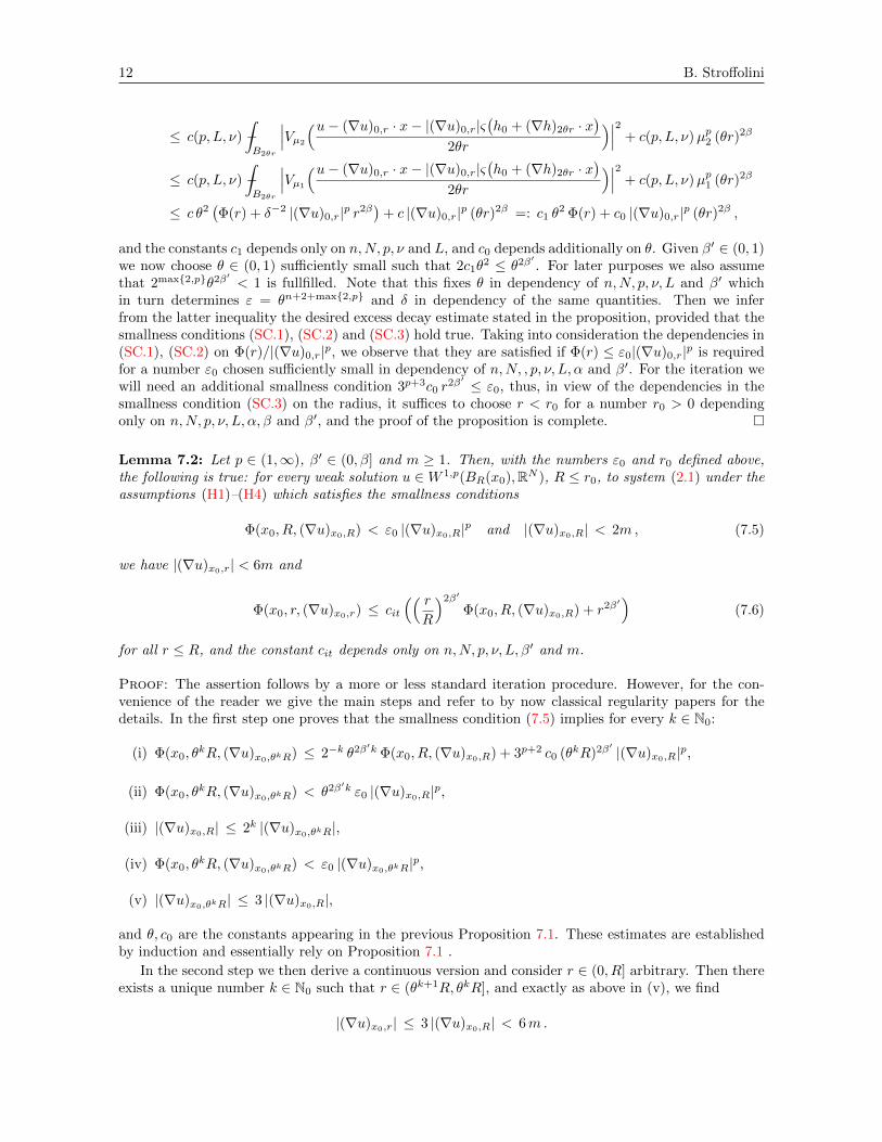
12 B. Stroffolini

≤ c(p, L, ν)

∫−B2θr

∣∣∣Vµ2

(u− (∇u)0,r · x− |(∇u)0,r|ς(h0 + (∇h)2θr · x

)2θr

)∣∣∣2 + c(p, L, ν)µp2 (θr)2β

≤ c(p, L, ν)

∫−B2θr

∣∣∣Vµ1

(u− (∇u)0,r · x− |(∇u)0,r|ς(h0 + (∇h)2θr · x

)2θr

)∣∣∣2 + c(p, L, ν)µp1 (θr)2β

≤ c θ2(Φ(r) + δ−2 |(∇u)0,r|p r2β

)+ c |(∇u)0,r|p (θr)2β =: c1 θ

2 Φ(r) + c0 |(∇u)0,r|p (θr)2β ,

and the constants c1 depends only on n,N, p, ν and L, and c0 depends additionally on θ. Given β′ ∈ (0, 1)we now choose θ ∈ (0, 1) sufficiently small such that 2c1θ

2 ≤ θ2β′ . For later purposes we also assumethat 2max2,pθ2β′ < 1 is fullfilled. Note that this fixes θ in dependency of n,N, p, ν, L and β′ whichin turn determines ε = θn+2+max2,p and δ in dependency of the same quantities. Then we inferfrom the latter inequality the desired excess decay estimate stated in the proposition, provided that thesmallness conditions (SC.1), (SC.2) and (SC.3) hold true. Taking into consideration the dependencies in(SC.1), (SC.2) on Φ(r)/|(∇u)0,r|p, we observe that they are satisfied if Φ(r) ≤ ε0|(∇u)0,r|p is requiredfor a number ε0 chosen sufficiently small in dependency of n,N, , p, ν, L, α and β′. For the iteration wewill need an additional smallness condition 3p+3c0 r

2β′ ≤ ε0, thus, in view of the dependencies in thesmallness condition (SC.3) on the radius, it suffices to choose r < r0 for a number r0 > 0 dependingonly on n,N, p, ν, L, α, β and β′, and the proof of the proposition is complete.

Lemma 7.2: Let p ∈ (1,∞), β′ ∈ (0, β] and m ≥ 1. Then, with the numbers ε0 and r0 defined above,the following is true: for every weak solution u ∈W 1,p(BR(x0),RN ), R ≤ r0, to system (2.1) under theassumptions (H1)–(H4) which satisfies the smallness conditions

Φ(x0, R, (∇u)x0,R) < ε0 |(∇u)x0,R|p and |(∇u)x0,R| < 2m, (7.5)

we have |(∇u)x0,r| < 6m and

Φ(x0, r, (∇u)x0,r) ≤ cit

(( rR

)2β′

Φ(x0, R, (∇u)x0,R) + r2β′)

(7.6)

for all r ≤ R, and the constant cit depends only on n,N, p, ν, L, β′ and m.

Proof: The assertion follows by a more or less standard iteration procedure. However, for the con-venience of the reader we give the main steps and refer to by now classical regularity papers for thedetails. In the first step one proves that the smallness condition (7.5) implies for every k ∈ N0:

(i) Φ(x0, θkR, (∇u)x0,θkR) ≤ 2−k θ2β′k Φ(x0, R, (∇u)x0,R) + 3p+2 c0 (θkR)2β′ |(∇u)x0,R|p,

(ii) Φ(x0, θkR, (∇u)x0,θkR) < θ2β′k ε0 |(∇u)x0,R|p,

(iii) |(∇u)x0,R| ≤ 2k |(∇u)x0,θkR|,

(iv) Φ(x0, θkR, (∇u)x0,θkR) < ε0 |(∇u)x0,θkR|p,

(v) |(∇u)x0,θkR| ≤ 3 |(∇u)x0,R|,

and θ, c0 are the constants appearing in the previous Proposition 7.1. These estimates are establishedby induction and essentially rely on Proposition 7.1 .

In the second step we then derive a continuous version and consider r ∈ (0, R] arbitrary. Then thereexists a unique number k ∈ N0 such that r ∈ (θk+1R, θkR], and exactly as above in (v), we find

|(∇u)x0,r| ≤ 3 |(∇u)x0,R| < 6m.

Partial Regularity results for degenerate elliptic systems 13

Moreover, in view of (i) and shifting Lemma, we get

Φ(x0, r, (∇u)x0,r) ≤(θkR

r

)n ∫−BθkR

(x0)

∣∣V|(∇u)x0,r|(∇u− (∇u)x0,r

)∣∣2≤ c(p) θ−n

∫−BθkR

(x0)

∣∣V|(∇u)x0,θ

kR|(∇u− (∇u)x0,θkR

)∣∣2≤ c(p) θ−n

(2−k θ2β′k Φ(x0, R, (∇u)x0,R) + 3p+2 c0 (θkR)2β′ |(∇u)x0,R|p

)≤ cit

(( rR

)2β′

Φ(x0, R, (∇u)x0,R) + r2β′),

and due to the dependencies of θ we have cit = cit(n,N, p, ν, L, β′,m). This completes the proof of the

excess decay estimate (7.6) and thus of the lemma.

As already mentioned before we derive an excess decay estimate for the degenerate situation wherethe mean value of ∇u on a ball BR(x0) is “small” with respect to the excess (in some sense thisassumption is equivalent to the system being degenerate). Duzaar and Mingione [14] had considered adegeneracy as the p-Laplace system, and they then concluded that approximate p-harmonicity allowsto find an excess-decay estimate. We here argue similarly, namely we show that if the system exhibitsa degeneracy as a system of Uhlenbeck-structure, then approximate a-harmonicity implies the desiredexcess-decay estimate. Nevertheless, our proof is slightly different in order to succeed in showing thatalso in the superquadratic situation one smallness condition on the mean value of ∇u (instead of anadditional second condition on a smaller ball) is sufficient to prove the decay estimate. In what follows,we denote by γ ∈ (0, 1) the exponent from the excess decay estimate in Proposition 3.1 for weak solutionsof systems with Uhlenbeck structure (meaning that the weak solution has Holder exponent 2γ/p in thesuperquadratic case and Holder exponent γ in the subquadratic case).

Proposition 7.3: Let p ∈ (1,∞). For every exponent γ′ ∈ (0,minγ, β) and every number κ > 0 thereexist constants τ ∈ (0, 1

4 ] and r1 < 1 depending on n,N, p, ν, L, γ, γ′, β and κ, and a constant ε1 > 0depending additionally on µ(·) such that the following is true: Let u ∈ W 1,p(Br(x0),RN ), r ≤ r1, be aweak solution to system (2.1) under the assumptions (H1)–(H5). If

κ |(∇u)x0,r|p ≤ Φ(x0, r, (∇u)x0,r) < ε1 (7.7)

is fullfilled, then we have

Φ(x0, τr, (∇u)x0,τr) ≤ τ2γ′ Φ(x0, r, (∇u)x0,r) . (7.8)

Proof: Without loss of generality we take x0 = 0, and we use the abbreviations Φ(r) = Φ(0, r, (∇u)0,r)and Ψ(r) = Ψ(0, r). From |(∇u)0,r|p ≤ κ−1Φ(r) we see for the superquadratic case p ≥ 2

Ψ(r) ≤ 2p−1

∫−Br

|∇u− (∇u)0,r|p + 2p−1 |(∇u)0,r|p ≤ 2p−1(1 + κ−1) Φ(r) ,

whereas in the subquadratic case we distinguish the cases where |∇u− (∇u)0,r| ≥ |(∇u)0,r| and wherethe opposite inequality holds true, and we obtain

Ψ(r) ≤ 2p−1

∫−Br

|∇u− (∇u)0,r|p + 2p−1 |(∇u)0,r|p

≤ 2p−1 22−p2

∫−Br

∣∣V|(∇u)0,r|(∇u− (∇u)0,r

)∣∣2 + 2p |(∇u)0,r|p ≤ 2p (1 + κ−1) Φ(r) .

Hence, in any case we getΨ(r) ≤ cΨ Φ(r) , (7.9)

14 B. Stroffolini

where we have set cΨ = 2p(1 + κ−1). In view of Lemma 6.2 on approximate a-harmonicity we have forevery t > 0 and every η ∈ C1

0 (Br,RN ):∣∣∣ ∫−Br

〈 ρx0(|∇u|)∇u,∇η 〉∣∣∣ ≤ cH

[tΨ(r)

p−1p + rβ Ψ(r)

p−1p +

Ψ(r)

µ(t)

]supBr

|∇η|

Now let τ ∈ (0, 14 ] to be specified later and define ε = τp+max1, p2 (n+2γ). Furthermore, let δ =

δ(n,N, p, ν, L, ε) ∈ (0, 1] be the constant according to the a-harmonic approximation with θ = n/(n+p):For all assumptions of Lemma 4.3 to be fullfilled it still remains to verify assumption (4.4). For this

purpose we fix t = t(L, δ) > 0 and a radius r1 = r1(L, δ, β) > 0 such that cHt ≤ δ/3 and cH rβ1 ≤ δ/3,

which in turn fixes µ(t). If we assume that the smallness condition

cH(cΨΦ(r))1/p

µ(t)≤ δ

3(SC.4)

holds, then, after application of Young’s inequality, u satisfies all assumption of Lemma 4.3, providedthat r ≤ r1. Consequently, there exists a a-harmonic map h ∈ W 1,p(Br,RN ) for a(z) = ρ0(|z|) z andwhich satisfies∫

−Br

|∇h|p ≤ c

∫−Br

|∇u|p and(∫−B

|V (∇u)− V (∇h)|2θ) 1θ ≤ ε

∫−2B

(|∇u|)p (7.10)

for a constant c depending only on p, ν and L. We here have used the fact that for all possible choicesof ρ satisfying the assumptions (G1)–(G3) the statement of Lemma 4.3 holds true with µ = 0 (andhence Vµ(z) = |z|(p−2)/2z) as well as a simple property of the V -function. In fact Caccioppoli andPoincare imply a higher integrability result for ∇u (see 5.2), so we can consider the previous smallnessassumption in this way:(∫

−B

|V (∇u)− V (∇h)|2)≤ ε

(∫−2B

|∇u|p+η) pp+η

+ cΨ(r)r2β (7.11)

Suppose that we start from Bτr. For the minimality of (∇u)0,τr we can consider any P ∈ RnN and usethe minimality of the shifted function:

Φ(τr) =

∫−Bτr

∣∣V|(∇u)0,τr|(∇u− (∇u)0,τr

)∣∣2≤ c(p)

∫−Bτr

∣∣V|P |(∇u− P )∣∣2 ≤ c(p)

∫−Bτr

∣∣V (∇u)− V (P ))∣∣2

≤ c(p)

∫−Bτr

∣∣V (∇u)− V (∇h))∣∣2 +

∫−Bτr

∣∣V (∇h)− V (P ))∣∣2 (7.12)

≤ c(p, L, ν)ετ−nΨ(r) + c(p, L, ν) [τ2γ+, (2τr)2β ]Ψ(r)

≤ c3(n,N, p, L, ν, κ)(τ2γ + (τr)2β

)Φ(r) . (7.13)

Here we have chosen P = (∇h)0,τr and applied the excess decay estimate stated in proposition 3.1.For a given exponent γ′ ∈ (0,minγ, β) we now fix τ ∈ (0, 1

4 ] such that

c3 τmin2γ,2β ≤ τ2γ′ . (SC.5)

Hence, τ is fixed in dependency of n,N, p, L, ν, γ, γ′, β and κ. The choice ε = τp+max1, p2 (n+2γ) furtherfixes δ – and therefore also t and the radius r1 – with exactly the same dependencies as those appearingin τ . We now remark that (SC.4) may be rewritten by

Φ(r) ≤ c−1Ψ

(δ µ(t)

3cH

)p= 2−p

κ

1 + κ

(δ µ(t)

3cH

)p.

Partial Regularity results for degenerate elliptic systems 15

For later purposes, we additionally assume that

Φ(r)1pτ−n/2

1− τγ′κp−22p + Φ(r)

1p

τ−n/p

1− τ2γ′/p≤ 1 . (SC.6)

Hence, we observe that these smallness conditions are fullfilled if we choose ε1 sufficiently small independency of the parameters stated in the proposition. This completes the proof.

Remark: We mention that the radius r appears in inequality (7.12) as a factor. Thus, we may replace(SC.5) by the following smallness condition concerning r and τ :

c3 rβ τ2β ≤ 1

2τ2β and c3 τ

2γp ≤ 1

2τ2β ,

where c3 = c3(n,N, p, L, ν, κ). This enables us to state the excess decay estimate also with exponentγ′ = β when β < γ.

Lemma 7.4 (Excess decay): Let p ∈ (1,∞). For every exponent γ′ ∈ (0,minγ, β) and m ≥ 1 thereexist ε1 = ε1(n,N, p, ν, L, γ, γ′, α, β, µ(·)) > 0 and a radius r2 = r2(n,N, p, ν, L, γ, γ′, α, β) > 0 such thatthe following is true: Let u ∈ W 1,p(BR(x0),RN ), R ≤ r2, be a weak solution to system (2.1) under theassumptions (H1)–(H5). If the smallness conditions

Φ(x0, R, (∇u)x0,R) < ε1 and |(∇u)x0,R| < m (7.14)

are fullfilled, then we have

Φ(x0, r, (∇u)x0,r) ≤ c(( r

R

)2γ′

Φ(x0, R, (∇u)x0,R) + r2γ′)

for all r ≤ R , (7.15)

and c depends on n,N, p, ν, L, γ, γ′, β, α and m.

Proof: We again take x0 = 0 and use the abbreviation Φ(R) = Φ(0, R, (∇u)0,R). Let γ′ ∈ (0,minγ, β),where γ is the exponent from Proposition 3.1, and choose β′ = γ′ in Lemma 7.2. This fixes two positiveconstants

ε0 = ε0(n,N, p, ν, L, α, γ′) ,

r0 = r0(n,N, p, ν, L, α, β, γ′) .

Furthermore, we set κ = ε0 and we find from Proposition 7.3 positive constants

τ = τ(n,N, p, ν, L, γ, γ′, β, α) ,

r1 = r1(n,N, p, ν, L, γ, γ′, β, α) ,

ε1 = ε1(n,N, p, ν, L, γ, γ′, β, α, µ(·)) .

We define r2 := minr0, r1. We next observe that (7.14) ensures that the second inequality in thesmallness assumption (7.7) required for the application of Proposition 7.3 is satisfied. We introduce theset of natural numbers

S :=n ∈ N0 : Φ(τnR) ≥ ε0 |(∇u)0,τnR|p

(we note that due to the different conditions in the excess-decay estimate [14, Proposition 4] we need -in contrast to [14, Lemma 13] – only one condition). In order to prove the desired excess decay estimatewe have to distinguish the cases where the mean values of ∇u is always small (i. e. where the system ispurely degenerate) and where the mean value for a certain radius (and then for every smaller radius)dominates the excess of ∇u:

Case S = N: By induction we prove for every k ∈ N0

Φ(τkR) < ε1 and Φ(τkR) ≤ τ2kγ′ Φ(R) . (7.16)

16 B. Stroffolini

For k = 0 these inequalities are trivially satisfied due to (7.14). Now, for a given k ∈ N0, we suppose(7.16)j for j ∈ 0, . . . , k. In view of k ∈ S we may apply Proposition 7.3 on the ball BτkR and we find

Φ(τk+1R) ≤ τ2γ′Φ(τkR) ≤ τ2(k+1)γ′Φ(R). Moreover, Φ(τk+1R) < ε1 follows from (7.16)0 and τ < 1.This shows that (7.16) is valid for k + 1 and therefore, for every k ∈ N0. For proving the excess decayestimate (7.15) we first infer from Lemma ??

Φ(r) =

∫−Br

∣∣V|(∇u)0,r|(∇u− (∇u)0,r

)∣∣2≤ c(p)

( rR

)−n ∫−BR

∣∣V|(∇u)0,R|(∇u− (∇u)0,R

)∣∣2 = c(p)( rR

)−nΦ(R) (7.17)

for all 0 < r ≤ R. For a continuous analogue of the decay estimate in (7.16) we now consider r ∈ (0, R]arbitrary. Then there exists a unique k ∈ N such that r ∈ (τk+1R, τkR], and using (7.16) and (7.17) weconclude

Φ(r) ≤ c(p)( r

τkR

)−nΦ(τkR) ≤ c(p) τ−n τ2kγ′ Φ(R) ≤ c(p) τ−n−2γ′

( rR

)2γ′

Φ(R) , (7.18)

and the statement of the lemma follows taking into account the dependencies of τ given above.Case S 6= N: We define k0 := minN \ S. We obtain Φ(τk0R) < ε0 |(∇u)τk0R|p by definition of k0,

and the calculations leading to (7.16) reveal

Φ(τkR) ≤ τ2kγ′ Φ(R) for every k ≤ k0 . (7.19)

Furthermore, we observe that (7.14) and (7.19) combined with the smallness condition (SC.6) ensurethat the mean values of ∇u remain uniformly bounded in the sense that we have |(∇u)0,τkR| < 2m forevery k ≤ k0: In the subquadratic case this can be seen as follows:

|(∇u)0,τkR| ≤ |(∇u)0,R|+k−1∑j=0

|(∇u)0,τjR − (∇u)0,τj+1R|

< m+ τ−np

k−1∑j=0

Φ(τ jR)1p + τ−

n2

k−1∑j=0

Φ(τ jR)12 |(∇u)0,τjR|

2−p2

≤ m+ τ−np (1− τ2γ′/p)−1 Φ(R)

1p + τ−

n2 (1− τγ

′)−1 Φ(R)

1p ε

p−22p

0 ≤ 2m.

In the superquadratic case instead, we find proceed analogously (but the third term in the sum doesnot appear) and get the same result. Hence, the assumptions of Lemma 7.2 are satisfied on the ballBτk0R. In view of (7.19) we thus infer for every r ∈ (0, τk0R]

Φ(r) ≤ cit

(( r

τk0R

)2γ′

Φ(τk0R) + r2γ′)≤ cit

(( rR

)2γ′

Φ(R) + r2γ′), (7.20)

where cit is the constant from Lemma 7.2 and depends only on n,N, p, ν, L, γ′ and m. To finish theproof of the excess decay estimate (7.15) it still remains to consider radii r ∈ (τk0R,R], but the assertionis then deduced easily from (7.19) following the line of arguments for the case S = N. Exactly as inthe proof of the excess decay result stated in [14], the integer k0 (which cannot be controlled and whichdepends on the point x0 under consideration) is not reflected in the dependencies of the constant cappearing in (7.15).

Remark: As mentioned in the introduction, the proof presented here simplifies slightly the one of [14,Lemma 13]. The key point here is the definition of the set S which was previously defined in a way suchthat the condition was required to hold on two subsequent balls (see the different smallness assumptions(7.7) and [14, (5.25)] in the excess decay estimate).

Partial Regularity results for degenerate elliptic systems 17

8 Proofs of the main results

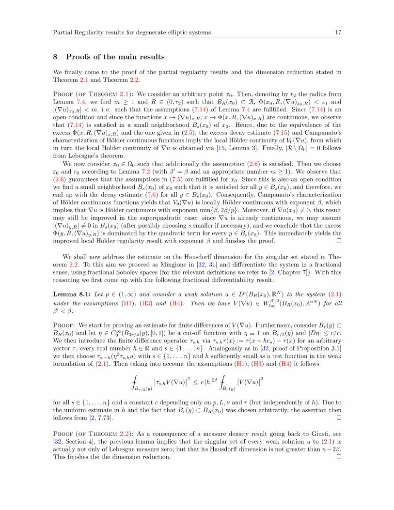
We finally come to the proof of the partial regularity results and the dimension reduction stated inTheorem 2.1 and Theorem 2.2.

Proof (of Theorem 2.1): We consider an arbitrary point x0. Then, denoting by r2 the radius fromLemma 7.4, we find m ≥ 1 and R ∈ (0, r2) such that BR(x0) ⊂ R, Φ(x0, R, (∇u)x0,R) < ε1 and|(∇u)x0,R| < m, i. e. such that the assumptions (7.14) of Lemma 7.4 are fullfilled. Since (7.14) is anopen condition and since the functions x 7→ (∇u)x,R, x 7→ Φ(x,R, (∇u)x,R) are continuous, we observethat (7.14) is satisfied in a small neighborhood Bs(x0) of x0. Hence, due to the equivalence of theexcess Φ(x,R, (∇u)x,R) and the one given in (2.5), the excess decay estimate (7.15) and Campanato’scharacterization of Holder continuous functions imply the local Holder continuity of V0(∇u), from whichin turn the local Holder continuity of ∇u is obtained via [15, Lemma 3]. Finally, |R \ Ω0| = 0 followsfrom Lebesgue’s theorem.

We now consider x0 ∈ Ω0 such that additionally the assumption (2.6) is satisfied. Then we chooseε0 and r0 according to Lemma 7.2 (with β′ = β and an appropriate number m ≥ 1). We observe that(2.6) guarantees that the assumptions in (7.5) are fullfilled for x0. Since this is also an open conditionwe find a small neighborhood Bs(x0) of x0 such that it is satisfied for all y ∈ Bs(x0), and therefore, weend up with the decay estimate (7.6) for all y ∈ Bs(x0). Consequently, Campanato’s characterizationof Holder continuous functions yields that V0(∇u) is locally Holder continuous with exponent β, whichimplies that ∇u is Holder continuous with exponent minβ, 2β/p. Moreover, if ∇u(x0) 6= 0, this resultmay still be improved in the superquadratic case: since ∇u is already continuous, we may assume|(∇u)y,R| 6= 0 in Bs(x0) (after possibly choosing s smaller if necessary), and we conclude that the excessΦ(y,R, (∇u)y,R) is dominated by the quadratic term for every y ∈ Bs(x0). This immediately yields theimproved local Holder regularity result with exponent β and finishes the proof.

We shall now address the estimate on the Hausdorff dimension for the singular set stated in The-orem 2.2. To this aim we proceed as Mingione in [32, 31] and differentiate the system in a fractionalsense, using fractional Sobolev spaces (for the relevant definitions we refer to [2, Chapter 7]). With thisreasoning we first come up with the following fractional differentiability result:

Lemma 8.1: Let p ∈ (1,∞) and consider a weak solution u ∈ Lp(BR(x0),RN ) to the system (2.1)

under the assumptions (H1), (H3) and (H4). Then we have V (∇u) ∈ W β′,2loc (BR(x0),RnN ) for all

β′ < β.

Proof: We start by proving an estimate for finite differences of V (∇u). Furthermore, consider Br(y) ⊂BR(x0) and let η ∈ C∞0 (B3r/4(y), [0, 1]) be a cut-off function with η ≡ 1 on Br/2(y) and |Dη| ≤ c/r.We then introduce the finite difference operator τs,h via τs,hτ(x) := τ(x+ hes)− τ(x) for an arbitraryvector τ , every real number h ∈ R and s ∈ 1, . . . , n. Analogously as in [32, proof of Proposition 3.1]we then choose τs,−h(η2τs,hu) with s ∈ 1, . . . , n and h sufficiently small as a test function in the weakformulation of (2.1). Then taking into account the assumptions (H1), (H3) and (H4) it follows∫

−Br/2(y)

∣∣τs,hV (∇u)∣∣2 ≤ c |h|2β

∫−Br(y)

∣∣V (∇u)∣∣2

for all s ∈ 1, . . . , n and a constant c depending only on p, L, ν and r (but independently of h). Due tothe uniform estimate in h and the fact that Br(y) ⊂ BR(x0) was chosen arbitrarily, the assertion thenfollows from [2, 7.73].

Proof (of Theorem 2.2): As a consequence of a measure density result going back to Giusti, see[32, Section 4], the previous lemma implies that the singular set of every weak solution u to (2.1) isactually not only of Lebesgue measure zero, but that its Hausdorff dimension is not greater than n−2β.This finishes the the dimension reduction.

18 B. Stroffolini

References

[1] E. Acerbi and N. Fusco, Regularity for minimizers of non-quadratic functionals: the case 1 < p < 2,J. Math. Anal. Appl. 140 (1989), 115–135.

[2] R. A. Adams, Sobolev Spaces, Academic Press, New York, 1975.

[3] L. Beck, B. Stroffolini, Regularity results for differential forms solving degenerate elliptic systems,Calc. Var. Partial Differential Equations 46 (2013), no. 3-4, 769-808.

[4] F. Browder, Nonlinear elliptic boundary value problems, Bull. Am. Math. Soc. 69 (1963), 862–874.

[5] M. Carozza, N. Fusco, and G. Mingione, Partial Regularity of Minimizers of Quasiconvex Integralswith Subquadratic Growth, Ann. Mat. Pura Appl. Ser. 4 175 (1998), 141–164.

[6] E. De Giorgi, Un esempio di estremali discontinue per un problema variazionale di tipo ellittico,Boll. Unione Mat. Ital., IV. 1 (1968), 135–137.

[7] L. Diening and F. Ettwein, Fractional estimates for non-differentiable elliptic systems with generalgrowth, Forum Math. 20 (2008), no. 3, 523–556.

[8] L. Diening and C. Kreuzer, Linear convergence of an adaptive finite element method for the p-laplacian equation, SIAM J. Numer. Anal. 46 (2008), no. 2, 614–638.

[9] L. Diening, J. Malek, and M. Steinhauer, On Lipschitz truncations of Sobolev functions (withvariable exponent) and their selected applications, ESAIM, Control Optim. Calc. Var. 14 (2008),no. 2, 211–232.

[10] L. Diening, B. Stroffolini, and A. Verde, Everywhere regularity of functionals with φ-growth,Manuscr. Math. 129 (2009), no. 4, 449–481.

[11] L. Diening, B. Stroffolini, and A. Verde, The ϕ-harmonic approximation and the regularity ofϕ-harmonic maps, J. Differential Equations 253 (2012), no. 7, 1943-1958.

[12] F. Duzaar and J. F. Grotowski, Optimal interior partial regularity for nonlinear elliptic systems:the method of A-harmonic approximation, Manuscr. Math. 103 (2000), 267–298.

[13] F. Duzaar, J. F. Grotowski, and M. Kronz, Regularity of almost minimizers of quasi-convex varia-tional integrals with subquadratic growth, Ann. Mat. Pura Appl. 11 (2005), no. 4, 421–448.

[14] F. Duzaar and G. Mingione, Regularity for degenerate elliptic problems via p-harmonic approxima-tion, Ann. Inst. Henri Poincare, Anal. Non Lineaire 21 (2004), no. 5, 735–766.

[15] F. Duzaar and G. Mingione, The p-harmonic approximation and the regularity of p-harmonic maps,Calc. Var. Partial Differ. Equ. 20 (2004), 235–256.

[16] F. Duzaar and G. Mingione, Second order parabolic systems, optimal regularity, and singular setsof solutions, Ann. Inst. Henri Poincare Anal. Non Lineaire 22 (2005), no. 6, 705–751.

[17] F. Duzaar and G. Mingione, Harmonic type approximation lemmas, J. Math. Anal. Appl. 352(2009), no. 1, 301–335.

[18] F. Duzaar and K. Steffen, Optimal interior and boundary regularity for almost minimizers to ellipticvariational integrals, J. Reine Angew. Math. 546 (2002), 73–138.

[19] J. Frehse, J. Malek, and M. Steinhauer, On analysis of steady flows of fluids with shear-dependentviscosity based on the Lipschitz truncation method, SIAM J. Math. Anal. 34 (2003), no. 5, 1064–1083.

Partial Regularity results for degenerate elliptic systems 19

[20] N. Fusco and J. E. Hutchinson, Partial regularity for minimisers of certain functionals havingnonquadratic grwoth, Ann. Mat. Pura Appl., IV. Ser. 155 (1989), 1–24.

[21] M. Giaquinta and G. Modica, Almost-everywhere regularity results for solutions of non linear ellipticsystems, Manuscr. Math. 28 (1979), 109–158.

[22] M. Giaquinta and G. Modica, Remarks on the regularity of the minimizers of certain degeneratefunctionals, Manuscr. Math. 57 (1986), 55–99.

[23] E. Giusti and M. Miranda, Sulla Regolarita delle Soluzioni Deboli di una Classe di Sistemi ElliticiQuasi-lineari, Arch. Rational Mech. Anal. 31 (1968), 173–184.

[24] E. Giusti and M. Miranda, Un esempio di soluzioni discontinue per un problema di minimo relativoad un integrale regolare del calcolo delle variazioni, Boll. Unione Mat. Ital., IV. Ser. 1 (1968), 219–226.

[25] C. Hamburger, Regularity of differential forms minimizing degenerate elliptic functionals, J. ReineAngew. Math. 431 (1992), 7–64.

[26] C. Hamburger, Quasimonotonicity, Regularity and Duality for Nonlinear Systems of Partial Dif-ferential Equations, Ann. Mat. Pura Appl. 169 (1995), 321–354.

[27] P.-A. Ivert, Regularitatsuntersuchungen von Losungen elliptischer Systeme von quasilinearenDifferentialgleichungen zweiter Ordnung, Manuscr. Math. 30 (1979), 53–88.

[28] J. Kristensen and G. Mingione, The Singular Set of Minima of Integral Functionals, Arch. RationalMech. Anal. 180 (2006), no. 3, 331–398.

[29] P. Marcellini, Everywhere regularity for a class of elliptic systems without growth conditions, Ann.Sc. Norm. Super. Pisa, Cl. Sci., IV. Ser. 23 (1996), no. 1, 1–25.

[30] P. Marcellini and G. Papi, Nonlinear elliptic systems with general growth, J. Differ. Equations 221(2006), no. 2, 412–443.

[31] G. Mingione, Bounds for the singular set of solutions to non linear elliptic systems, Calc. Var.Partial Differ. Equ. 18 (2003), no. 4, 373–400.

[32] G. Mingione, The Singular Set of Solutions to Non-Differentiable Elliptic Systems, Arch. RationalMech. Anal. 166 (2003), 287–301.

[33] G. Mingione, Regularity of minima: an invitation to the Dark Side of the Calculus of Variations,Appl. Math. 51 (2006), no. 4, 355–425.

[34] T. Schmidt, Regularity of minimizers of w1,p-quasiconvex variational integrals with (p, q)-growth,Calc. Var. Partial Differ. Equ. 32 (2008), no. 1, 1–24.

[35] T. Schmidt, Regularity theorems for degenerate quasiconvex energies with (p, q)-growth, Adv. Calc.Var. 1 (2008), no. 3, 241–270.

[36] P. Tolksdorf, Everywhere-regularity for some quasilinear systems with a lack of ellipticity, Ann.Mat. Pura Appl., IV. Ser. 134 (1983), 241–266.

[37] K. Uhlenbeck, Regularity for a class of nonlinear elliptic systems, Acta Math. 138 (1977), 219–240.