ORIGINAL PAPER

Parsimonious use of indicators for evaluating sustainabilitysystems with multivariate statistical analyses

Rajib Mukherjee • Debalina Sengupta •

Subhas K. Sikdar

Received: 11 January 2013 / Accepted: 30 March 2013 / Published online: 16 April 2013

� Springer-Verlag Berlin Heidelberg (outside the USA) 2013

Abstract Indicators are commonly used for evaluating

relative sustainability for competing products and pro-

cesses. When a set of indicators is chosen for a particular

system of study, it is important to ensure that they vary

independently of each other. Often, the number of indica-

tors characterizing a chosen system may be large. It is

essential to select the most important indicators from a

large set so that a dependable bias-free analysis can be

done using the reduced set of indicators. In this paper, we

propose the use of principal component analysis (PCA)

along with the partial least square-variable importance in

projection (PLS-VIP) method to ensure that the explicit or

tacit assumption of the independence of the chosen indi-

cators is valid. We have used two case studies to demon-

strate successful use of these two methods for parsimonious

use of indicators for sustainability analysis of systems.

Keywords Principal component analysis (PCA) � Partial

least square–variable importance in projection (PLS–VIP) �Sustainability � Indicators � Multivariate statistical analysis

Introduction

It is generally agreed that systems should be evaluated for

their relative sustainability using quantitative indicators or

metrics, terms that are used here interchangeably. Typi-

cally, indicators for the purpose of sustainability

assessment are chosen using the standard Bruntland model

of the three sustainability domains of environment, econ-

omy, and society. There have been several attempts to

evaluate industrial systems for sustainability with quanti-

tative indicators (IChemE 2002; AIChE 2003; Shonnard

et al. 2003; Zhou et al. 2012). A standard list of indicators

that applies to all systems of concern, however, cannot

exist as the systems differ from each other in system type,

scale, and properties. Nevertheless, even when the chosen

indicators are deemed commensurate for a particular sys-

tem of study, it is important to recognize that they should

be independently variable. This feature is important

because it helps in removing bias introduced from multiple

uses of similar indicators. When the number of indicators is

large, the task of sorting them into a necessary and suffi-

cient number of metrics is essential for dependable

analyses.

Even when the number of indicators is limited, comparing

alternatives for relative sustainability can still be difficult

owing to very frequent occurrences of the favored option not

enjoying superior numerical values for all chosen indicators.

It was demonstrated earlier that aggregating the indicators

into a single index is an easy way to enable decision making

on relative sustainability (Sikdar 2009; Sikdar et al. 2012).

Two methods were successfully used, one based on Euclid-

ian distances of alternate candidates from a common refer-

ence point and the other on geometric mean of the ratios of

individual indicator values of a candidate option and those of

the chosen reference. Both methods are based on the con-

sideration that a multidimensional indicator space charac-

terizes the system and the various system alternatives are

points in that space. The task is then to determine the distance

between these point systems and a properly chosen reference

point. Relative distances are quantitative representations of

relative sustainability.

Rajib Mukherjee and Debalina Sengupta: ORISE Fellow at EPA.

R. Mukherjee � D. Sengupta � S. K. Sikdar (&)

National Risk Management Research Laboratory, United States

Environmental Protection Agency, Cincinnati, OH 45268, USA

e-mail: sikdar.subhas@epa.gov

123

Clean Techn Environ Policy (2013) 15:699–706

DOI 10.1007/s10098-013-0614-6

However, the objective of making reliable decisions on

relative sustainability can be strengthened with a suitable

methodology for identifying those indicators that are nec-

essary and sufficient for analyses. For this purpose, we

need to identify if some of the indicators are correlated and

whether all the indicators are important for describing the

options. To address this, two multivariate statistical anal-

ysis methods were used.

The first method is the principal component analysis

(PCA). Its use in sustainability analyses was motivated by

the desire to see if the explicit or tacit assumption of the

independence of the chosen indicators is valid, i.e., if some of

the indicators are derivatives of other indicators (i.e., cor-

related) and therefore are not measuring independent attri-

butes of the system under study. PCA treats the indicator

datasets as eigenvalue problems and proceeds to find the

corresponding eigenvectors, also known as the principal

components. While PCA is capable of selecting a set of

unique indicators which are not correlated, it, however,

cannot differentiate the relative importance of the indicators,

for which the second method, the partial least square–vari-

able importance in projection (PLS–VIP) method, can be

used. Unlike PCA, PLS–VIP is a supervised model where an

overall pattern of the datasets is required. We extract features

from the data that are trained with inputs (indicators or

metrics) along with their corresponding outputs (aggregate

index). This work provides a description of these two

methods and illustrates their use in making decisions on

relative sustainability with case studies from the literature.

Theoretical considerations

Let us consider a system for which m is the number of

options that exist for attaining superior sustainability out-

come for the system, and the number of indicators under

consideration is n. Thus, in an n-dimensional indicator

space, every option is represented as a point. The objective

is to determine the most sustainable choice among the

options and additionally to determine how many of the

n indicators are necessary in deciding on the best option,

the next best option, and so on by reducing the dimen-

sionality of the system under consideration. Moreover, we

would also like to know which of the indicators is the most

important, the next most important, and so on in deter-

mining the sustainability outcome. In this analysis, the

indicators judged not essential are either insignificant or

redundant. When following the sustainability profile of a

system over time, m will represent the different states of

the system at identified points in time.

As an example, we could think of a product for which

m different processes can be considered. Or, to track

temporal sustainability outcome, an ecosystem can be

monitored over several years. It is tacitly assumed in this

formulation that the chosen indicators take into account all

necessary features of the system such that the system can

be completely described by the values of the indicators.

The multivariate statistical methods used to satisfy the

objective include the PCA together with the PLS–VIP

method. These two multivariate analyses will describe a

method of identifying sufficiency of a set of indicators and

of finding their relative importance in obtaining the sus-

tainability of different options. To carry out the analysis,

statistical software package XLStat was used, which is

available as an add-on to Microsoft Excel�.

Aggregate index

We start by recognizing a dataset consisting of m 9 n data

points, m being the number of options, each option being

characterized by the values of n different indicators. A

Euclidean distance can be defined by pairwise comparing

an option with a reference option, which can be either

synthetically constructed or chosen from among the real

options. Thus, for option Y to be compared with reference

option X0, De can be defined as (Sikdar et al. 2012)

De ¼

ffiffiffiffiffiffiffiffiffiffiffiffiffiffiffiffiffiffiffiffiffiffiffiffiffiffiffiffiffiffiffiffiffiffiffiffiffiffiffiffiffiffiffiffi

X

n

j

cj

yj � xj0

� �

yj � xj0

� �

max

" #2v

u

u

t ð1Þ

where yj is the value of the jth indicator for option Y, and

the corresponding value for the reference option is xj0. De

as written in Eq. 1 has been normalized by the quantity

(yj–xj0)max to make the difference dimensionless. The

presence of cj allows us to insert a weighting factor for

each indicator j, if we have a method of making that

choice. For the illustrative examples of the analysis

methodology in this work, we always used cj as 1.0. Since

each pairwise comparison involves n indicators, De is the

distance of Y from X0 in the n-dimensional indicator space.

The greater the distance of Y from X0, the more unsus-

tainable the option is.

For similar pairwise comparisons, the alternate aggre-

gate index D is the geometric mean of the ratios of jth

indicator values of option Y to those values of option X0

and is given by Eq. 2.

D ¼Y

n

j

cj y0j

.

x0j

� �h i

!1=n

y0j ¼ yj � xj0 � Coffset

� �

x0j ¼ xj � xj0 � Coffset

� �

ð2Þ

where y0j and x0j were obtained by shifting the differences by

a constant quantity Coffset. As defined, D is naturally

dimensionless.

700 R. Mukherjee et al.

123

By repeating this calculation for each option, we will get

n such aggregate indices. These distances will be measures

of sustainability. In an inter-comparison among the

options, the smaller the distance an option has, the closer is

that option to sustainability, thus giving us a handle on

relative sustainability of the options. A synthetic reference

system can be created by just picking the most desirable

indicator values in the dataset.

The idea of the reference option in De calculation is to

transform the dataset to avoid occurrence of negative data

points, and that of the offset in D calculation is to avoid

having 0 or infinity in the transformed data. The weighting

factor cj allows use of weighting preference (usually a

societal choice) of any of the indicators in comparison to

others. The D or De by themselves offers two ways of

making sustainability decisions. The process or product

option having a smaller D or De value is considered to be

more sustainable, in accordance with the convention that

each indicator is fashioned in a way in which lower

numerical values are more desirable than higher ones.

Principal component analysis (PCA)

PCA designs n-dimensional unit vectors (q’s) onto which

the n-dimensional input data vectors are projected. This

process creates a transformation matrix of the original data

matrix X called the correlation matrix, R (n 9 n), such that

the following eigenvalue problem can represent the entire

dataset.

RQ ¼ DQ ð3Þ

where Q is an n x n matrix containing the unit eigenvector

q’s, D is the n 9 1 vector of the eigenvalues of the matrix

R. The n eigenvalues (k’s, elements of vector D) are

arranged in descending order. The sum of the eigenvalues

accounts for the total variability of the data. The percent

contribution of an eigenvalue (kj) toward total variability

can be expressed as kj

,

P

n

j

kj

!

� 100.

The matrix of eigenvectors, Q, denotes the direction of

the principal components (the direction of variability). The

most important eigenvectors indicate how many principal

components from the possible total of n need to be used to

account for the overwhelming portion of the data vari-

ability. In most cases, two or three principal components

are sufficient to account for most of the variability. Each

principal component represents all the input variables (in

our case, the indicators are the variables). Choosing a few

of these principal components merely is an exercise in

looking at the data from several different angles to capture

most of the variability of the data in order to reduce the

dimensionality of the data.

Mapping square roots of eigenvalues kj on to the

eigenvector matrix Q, we obtain the loading matrix L,

given in Eq. 4.ffiffiffiffi

Dp

Q ¼ L ð4Þ

From the product of the data matrix X with the loading

matrix L, we obtain the score matrix T, which is given in

Eq. 5.

XL ¼ T ð5Þ

Each element of the loading matrix, belonging to a

principal component, denotes the loading of an indicator in

the direction of that principal component. In a reduced

subspace of two principal components, we can obtain a plot

that shows loadings of each indicator. Indicators that form

clusters on such a plot are correlated. In our analysis, this

process is repeated with more principal components until

the chosen principal components cover [95 % of the data

variability.

Partial least squares–variable importance in projection

(PLS–VIP)

While PCA can be used to identify possible correlation of

the indicators, it does not help in identifying the relative

importance of the indicators in evaluating sustainability

options. For this purpose, we have used the PLS–VIP

method. The PLS–VIP method needs a response matrix,

which in our case is the vector of the aggregate index (D or

De) for options considered (process or product). The limi-

tation of using all of the original indicators in the aggregate

index calculation is that in these calculations, all indicators

are assumed to be important. PLS–VIP was used to

strengthen the sustainability analysis by reducing the

dimensionality of the indicator space and eliminating from

analysis those indicators that, however important they seem

on first glance, add little value to decision making.

PLS–VIP is a multivariate regression method based on

projecting the information from a data space of a larger

number of variables into that with a smaller number of

variables. The number of variables (indicators in our case)

is reduced in a way such that variations in the values of the

indicators are most likely to be reflected in the response

matrix. The PLS method uses the loadings (L) and score

(T) of the original data matrix X (as given in Eq. 4 and

Eq. 5) and the aggregate index vector De (as given in

Eq. 1).

Using the score of the data matrix X, PLS regression

develops a regression model between X and De. In a

reduced subspace of principal components of a dimension

where a B n, n being the total number of principal com-

ponents, X can be written as (Cinar et al. 2007)

Indicators for evaluating sustainability systems 701

123

X ¼ TLT þ E ¼X

a

j¼1

tjlTj þ E ð6Þ

where T is the score matrix, L is the loading matrix, and E

is the residual matrix of the data matrix X. The score matrix

T can also be related to the response vector De through a

regression matrix b as

De ¼ TbT þ F ð7Þ

where F is the residual vector of De. Each option vector x

from X can be related to the score vector tj through weight

vectors wj as

tj ¼ wTj xi ð8Þ

The variable importance in projection for a particular

indicator k, VIPk, is calculated using the regression

coefficient bj from the regression matrix b, weight vector

wj, and score vector tj as

VIPk ¼

ffiffiffiffiffiffiffiffiffiffiffiffiffiffiffiffiffiffiffiffiffiffiffiffiffiffiffiffiffiffiffiffiffiffiffiffiffi

n

P

a

j¼1

b2j tT

j tjwkj

wjk k

� �2

P

a

j¼1

b2j tT

j tj

v

u

u

u

u

u

u

t

ð9Þ

where wkj is the kth element of the wj vector.

PLS–VIP is used to identify the importance of each

indicator in characterizing the system, which has the

options, which are alternative solutions. Indicators with

low VIP scores have little power in characterizing a sys-

tem, and those with the highest VIP scores contribute the

most in the PLS model to characterizing it. The average of

squared VIP scores equals 1. A VIP score greater than one

is generally used as a criterion for variable selection

(Chong and Jun 2005).

Evaluation of sustainability systems

The theory of identifying correlated indicators and finding

their relative importance is applied to two different data-

sets. The first one is from a Fender case study and the next

one is from a case study based on auto shredder residue

(ASR) treatment strategy (Saur et al. 2000; Vermeulen

et al. 2012; Sikdar et al. 2012). It needs repeating here that

before launching the PLS–VIP analysis, we will have

already established relative sustainability using the D or

De, based on using all the indicators. The following anal-

ysis is directed to finding how many and which indicators

are minimally necessary for sound sustainability decisions.

Fender case study

The Fender case study dataset (Saur et al. 2000) comprises

five different automobile Fender options made of steel,

aluminum, and three different plastics formulations (PC/

PBT, PP/EPDM, PPO/PA), characterized by 12 different

indicators for resources, energy, water use (Water), waste,

global warming potential (GWP), eutrophication potential

(EP), ozone depletion potential (ODP), smog formation

potential (PCOP), ecotoxicity (EcoTox), acidification

potential (AP), human toxicity air (Htox air), and human

toxicity water (Htox water). To guide ourselves at this stage,

we calculated the relative sustainability signatures of the five

products using Eq. 1 for the Euclidean distance index De

using all 12 indicators. The De results already informed us

(Sikdar et al. 2012) of the relative sustainability of all these

products, but they did not inform us of the relative impor-

tance of the indicators and if there is any indicator redun-

dancy. The aggregate index analysis showed us that using

twelve indicators, the Fender formulation identified as

Energy

Resources

Water

GWP

ODPAP

EP

PCOP

Htox air

Htox Water

EcoTox

Waste

-1

-0.75

-0.5

-0.25

0

0.25

0.5

0.75

1

-1 -0.75 -0.5 -0.25 0 0.25 0.5 0.75 1

P2

(28.

06 %

)

P1 (49.38 %)

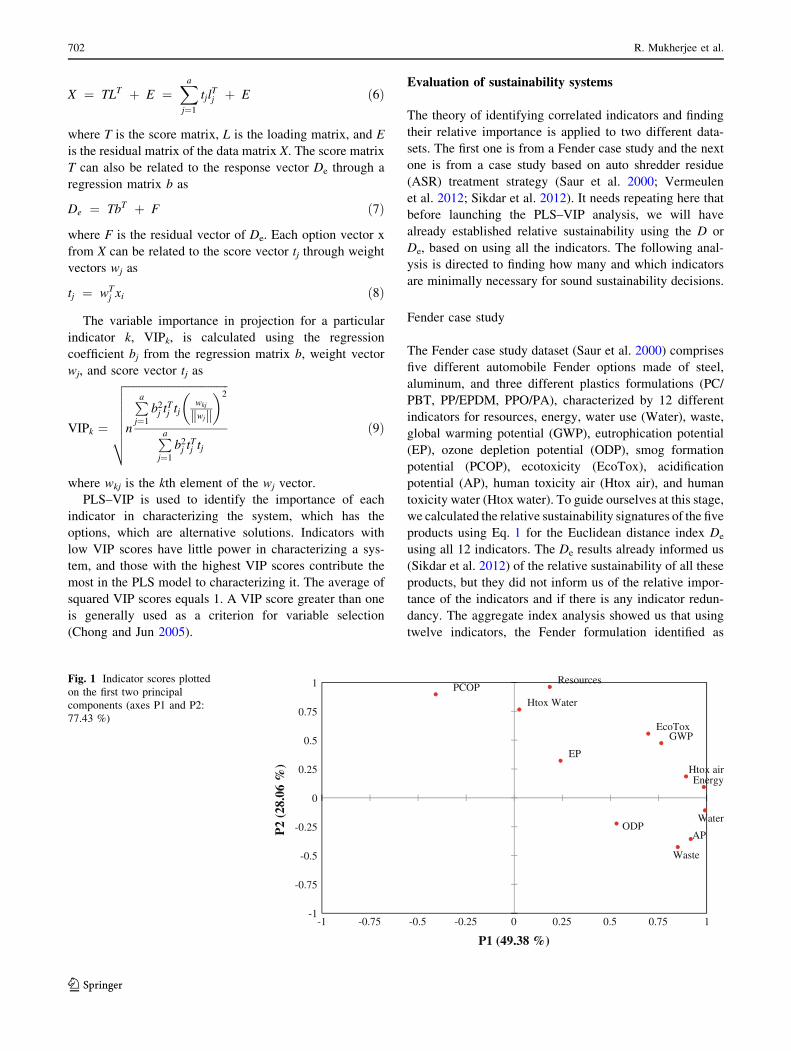
Fig. 1 Indicator scores plotted

on the first two principal

components (axes P1 and P2:

77.43 %)

702 R. Mukherjee et al.

123

PP/EPDM was the most sustainable of the five Fender

options. If we can establish the minimum number of indi-

cators that must be used for the sustainability analysis, we

would have to recompute the De values for a decision on

relative sustainability. First PCA and then PLS–VIP methods

were used to reduce the indicator space for this case study.

We start by performing PCA on the 5 9 12 dataset for

Fender options and indicators characterizing them. The first

two principal components (denoted by axes P1 and P2)

capture 78 % of the covariance of the original data and the

first three principal components (denoted by axes P1, P2,

and P3) capture[95 % of the covariance of the data. Two

separate plots are used to show the loadings of the indicators

on the principal components. The first plot is done with the

first two principal components shown in Fig. 1 and the

Energy

Resources

Water

GWP

ODP

AP

EP

PCOP

Htox airHtox Water

EcoTox

Waste

-1

-0.75

-0.5

-0.25

0

0.25

0.5

0.75

1

-1 -0.75 -0.5 -0.25 0 0.25 0.5 0.75 1

P3

(18.

74 %

)

P2 (28.06 %)

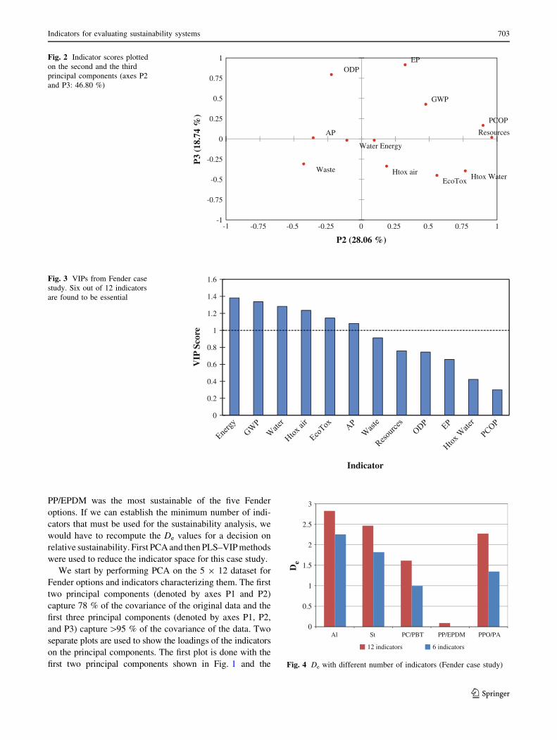
Fig. 2 Indicator scores plotted

on the second and the third

principal components (axes P2

and P3: 46.80 %)

0

0.2

0.4

0.6

0.8

1

1.2

1.4

1.6

VIP

Sco

re

Indicator

Fig. 3 VIPs from Fender case

study. Six out of 12 indicators

are found to be essential

0

0.5

1

1.5

2

2.5

3

Al St PC/PBT PP/EPDM PPO/PA

De

12 indicators 6 indicators

Fig. 4 De with different number of indicators (Fender case study)

Indicators for evaluating sustainability systems 703

123

second plot is done with the second and third principal

components shown in Fig. 2. Figures 1 and 2 show the

contributions of the indicators to the overall covariance of

the dataset. When the factor (i.e., indicator) loadings over-

lap, the contributions are exactly the same. This implies that

when they are close, the contributions are roughly similar.

Neither Fig. 1 nor Fig. 2 shows closeness or overlap of the

indicators. Thus, in this particular case, the PCA shows that

the indicators are not strongly correlated. Hence, we can

conclude that there is no redundancy in our choice of indi-

cators to describe the sustainability of the systems.

Next, we used PLS–VIP analysis to determine indicator

sufficiency and relative importance of the indicators. They

were calculated using Eq. 9. The vector of the aggregated

indices, De, was used as the response vector. The first three

principal components, accounting for over 95 % of the

covariance of the data, were used for the VIP calculation.

Results from the analysis are shown in Fig. 3. This figure

shows that first six indicators (Energy, GWP, Water, Htox

air, EcoTox, and AP), for which VIP values are C1.0,

provide indicator sufficiency. The energy use indicator is

the most important of the chosen indicators, followed by

GWP, water, and so on to determine relative sustainability.

To demonstrate that this choice of sufficient indicators is

reasonable for enhanced decision making for sustainable

systems, we recalculate De with the reduced set of indi-

cators. When the first six important indicators with VIP

score [1.0 are used for De calculation, the Fender formu-

lation PP/EPDM was again found to be the most sustain-

able option followed by PC/PBT, PPO/PA, St, and Al.

Figure 4 shows illustratively that the result remains

unchanged by including more indicators up to all 12 indi-

cators. Thus, we can make two decisions here. First, six

indicators along with their relative significance are suffi-

cient for the analysis. Second, PP/EPDM was the most

sustainable option. This decision is contingent on the

assumption that the researchers who did the original study

(Saur et al. 2000) did not leave out any important indicator

from consideration.

Auto shredder residue (ASR) case study

A similar analysis was conducted on the data from the ASR

case study (Vermeulen et al. 2012). The data comprise four

different process options for treatment of auto shredder resi-

due: (1) landfilling, (2) recycling of some metals and some

plastics with landfilling the rest (Recycle ? Landfill), (3)

energy recovery, and (4) recycling of some metals and some

plastics, recovering energy from the rest (Recycle ? Energy

Recovery). These options were evaluated using nine indica-

tors for energy intensity (EI), material intensity (MI), water

consumption (WC), land use (LU), global warming short term

(GWST), global warming long term (GWLT), human toxicity

short term (HTST), human toxicity long term (HTLT), and

treatment costs (TC). Vermeulen et al. concluded that the

Recycle ? Energy Recovery option was the most sustainable

option, whereas landfilling was least sustainable.

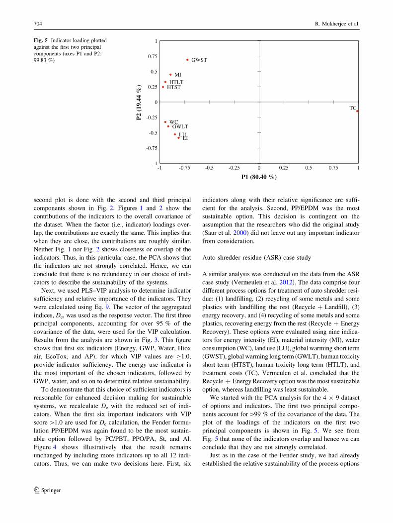
We started with the PCA analysis for the 4 9 9 dataset

of options and indicators. The first two principal compo-

nents account for[99 % of the covariance of the data. The

plot of the loadings of the indicators on the first two

principal components is shown in Fig. 5. We see from

Fig. 5 that none of the indicators overlap and hence we can

conclude that they are not strongly correlated.

Just as in the case of the Fender study, we had already

established the relative sustainability of the process options

EI

MI

WC

LU

GWST

GWLT

HTSTHTLT

TC

-1

-0.75

-0.5

-0.25

0

0.25

0.5

0.75

1

P2

(19.

44 %

)

P1 (80.40 %)

-1 -0.75 -0.5 -0.25 0 0.25 0.5 0.75 1

Fig. 5 Indicator loading plotted

against the first two principal

components (axes P1 and P2:

99.83 %)

704 R. Mukherjee et al.

123

by computing the De values, before launching PCA and

PLS–VIP analyses. That analysis told us that Recy-

cle ? Energy Recovery was the most sustainable of the

options, when all nine indicators were used. Recy-

cle ? Energy Recovery, however, was slightly better by De

values than the Recycle ? Landfill option. For engineering

purposes, though, they can be considered equivalent. Only

the decision makers can choose the option best suited to

local conditions based on factors not included in this

analysis. The other two options were significantly worse

and should not be chosen, from a sustainability viewpoint.

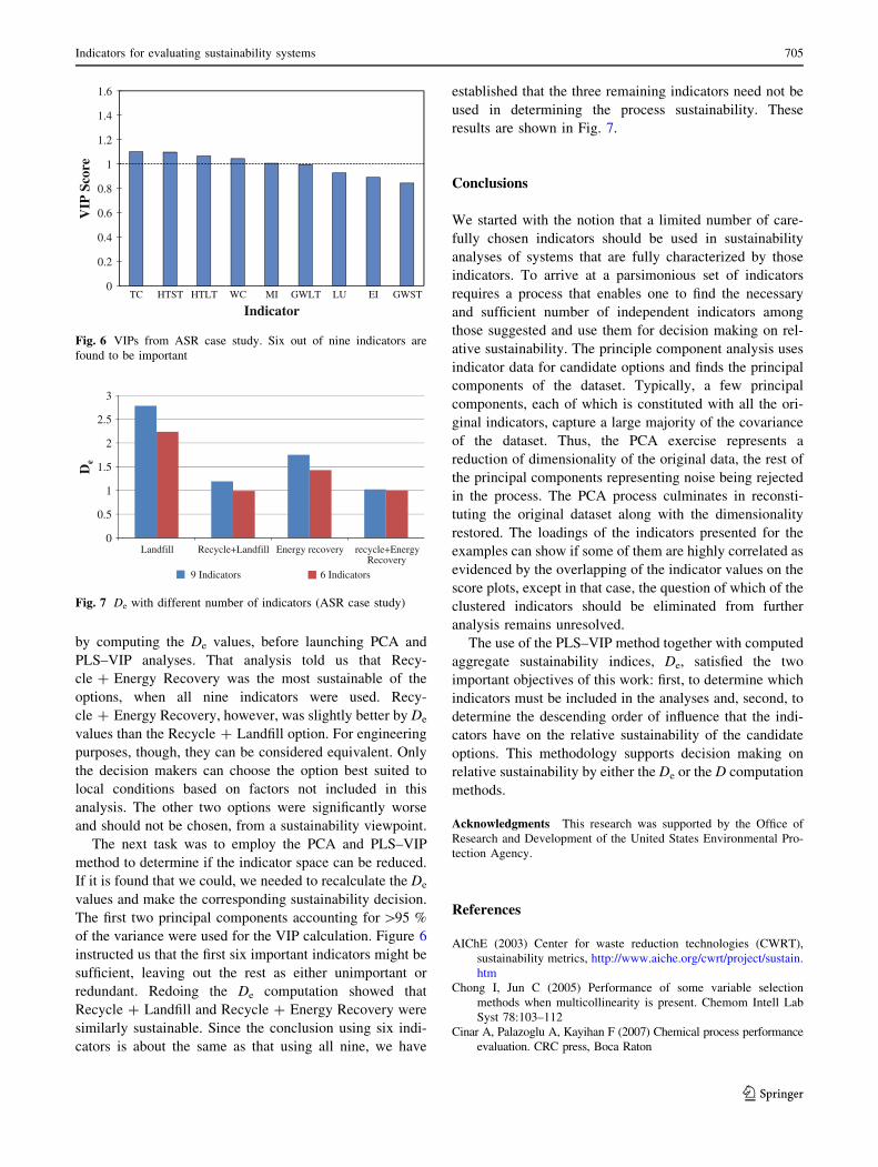
The next task was to employ the PCA and PLS–VIP

method to determine if the indicator space can be reduced.

If it is found that we could, we needed to recalculate the De

values and make the corresponding sustainability decision.

The first two principal components accounting for [95 %

of the variance were used for the VIP calculation. Figure 6

instructed us that the first six important indicators might be

sufficient, leaving out the rest as either unimportant or

redundant. Redoing the De computation showed that

Recycle ? Landfill and Recycle ? Energy Recovery were

similarly sustainable. Since the conclusion using six indi-

cators is about the same as that using all nine, we have

established that the three remaining indicators need not be

used in determining the process sustainability. These

results are shown in Fig. 7.

Conclusions

We started with the notion that a limited number of care-

fully chosen indicators should be used in sustainability

analyses of systems that are fully characterized by those

indicators. To arrive at a parsimonious set of indicators

requires a process that enables one to find the necessary

and sufficient number of independent indicators among

those suggested and use them for decision making on rel-

ative sustainability. The principle component analysis uses

indicator data for candidate options and finds the principal

components of the dataset. Typically, a few principal

components, each of which is constituted with all the ori-

ginal indicators, capture a large majority of the covariance

of the dataset. Thus, the PCA exercise represents a

reduction of dimensionality of the original data, the rest of

the principal components representing noise being rejected

in the process. The PCA process culminates in reconsti-

tuting the original dataset along with the dimensionality

restored. The loadings of the indicators presented for the

examples can show if some of them are highly correlated as

evidenced by the overlapping of the indicator values on the

score plots, except in that case, the question of which of the

clustered indicators should be eliminated from further

analysis remains unresolved.

The use of the PLS–VIP method together with computed

aggregate sustainability indices, De, satisfied the two

important objectives of this work: first, to determine which

indicators must be included in the analyses and, second, to

determine the descending order of influence that the indi-

cators have on the relative sustainability of the candidate

options. This methodology supports decision making on

relative sustainability by either the De or the D computation

methods.

Acknowledgments This research was supported by the Office of

Research and Development of the United States Environmental Pro-

tection Agency.

References

AIChE (2003) Center for waste reduction technologies (CWRT),

sustainability metrics, http://www.aiche.org/cwrt/project/sustain.

htm

Chong I, Jun C (2005) Performance of some variable selection

methods when multicollinearity is present. Chemom Intell Lab

Syst 78:103–112

Cinar A, Palazoglu A, Kayihan F (2007) Chemical process performance

evaluation. CRC press, Boca Raton

0

0.2

0.4

0.6

0.8

1

1.2

1.4

1.6

TC HTST HTLT WC MI GWLT LU EI GWST

VIP

Sco

re

Indicator

Fig. 6 VIPs from ASR case study. Six out of nine indicators are

found to be important

0

0.5

1

1.5

2

2.5

3

Landfill Recycle+Landfill Energy recovery recycle+EnergyRecovery

De

9 Indicators 6 Indicators

Fig. 7 De with different number of indicators (ASR case study)

Indicators for evaluating sustainability systems 705

123

IChemE (2002) Sustainability metrics, http://www.icheme.org/com-

munities/subject_groups/sustainability/*/media/Documents/

Subject%20Groups/Sustainability/Newsletters/Sustainability%20

Metrics.ashx

Saur C, Fava J, Spatari S (2000) Life cycle engineering case study:

automotive Fender designs. Environ Prog 19(2):72–82

Shonnard DR, Kirchner A, Saling P (2003) Industrial applications

using BASF eco-efficiency analysis: perspectives on green

engineering principles. Environ Sci Technol 37:5340–5348

Sikdar SK (2009) On aggregating multiple indicators into a single

metric for sustainability. Clean Tech Environ Policy 11:157–161

Sikdar SK, Sengupta D, Harten P (2012) More on aggregating

multiple indicators into a single index for sustainability analyses.

Clean Tech Environ Policy 14:765–773

Vermeulen I, Block C, Van Caneghem J, Dewulf W, Sikdar S,

Vandecasteele C (2012) Sustainability assessment of industrial

waste treatment processes. The case of automotive shredder

residue. Resour Conserv Recycle 69:17–28

Zhou L, Tokos H, Krajnc D, Yang Y (2012) Sustainability

performance evaluation in industry by composite sustainability

index. Clean Technol Environ Policy 14:789–803

706 R. Mukherjee et al.

123