parametric study on the seismic performance of typical ..._yuling_thesis.pdf · parametric study on...

Parametric Study on the Seismic Performance

of Typical Highway Bridges in Canada

Yuling Gao

A Thesis

in

The Department

of

Building, Civil and Environmental Engineering

Presented in Partial Fulfillment of the Requirements

for the Degree of Master of Applied Science (Civil Engineering) at

Concordia University

Montreal, Quebec, Canada

September 2014

© YULING GAO, 2014

Concordia University

School of Graduate Studies

This is to certify that the thesis prepared

By: Yuling Gao

Entitled: Parametric Study on the Seismic Performance of Typical Highway Bridges

in Canada

and submitted in partial fulfillment of the requirements for the degree of

Master of Applied Science (Civil Engineering)

complies with the regulations of the University and meets the accepted standards with

respect to originality and quality.

Signed by the final examining committee:

Dr. A. M. Hanna Chair

Dr. A. Bhowmick Examiner

Dr. Y. Zeng Examiner

Dr. L. Lin Supervisor

Approved by ________________________________________________

Chair of Department or Graduate Program Director

________________________________________________

Dean of Faculty

Date _________________________________

i

Abstract

Parametric Study on the Seismic Performance of Typical Highway Bridges in Canada

Yuling Gao

Earthquakes are one of the main natural hazards that have caused devastations to

bridges around the world. Given the observations from past earthquakes, substantial analytical

and experimental research work related to bridges has been undertaken in Canada and other

countries. The analytical research is focussed primarily on the prediction of the seismic

performance of existing bridges. It includes bridge-specific investigations which are mainly

conducted using deterministic approach, and investigations of bridge portfolios which are

based on probabilistic approach. In both cases, nonlinear time-history analyses are extensively

used. To conduct analysis on a given bridge, analytical (i.e., computational) model of the

bridge is required. It is known that the seismic response predictions depend greatly on the

accuracy of the input of the modeling parameters (or components) considered in the bridge

model.

The objective of this study is to investigate the effects of the uncertainties of a number

of modeling parameters on the seismic response of typical highway bridges. The parameters

considered include the superstructure mass, concrete compressive strength, yield strength of

the reinforcing steel, yield displacement of the bearing, post-yield stiffness of the bearing,

plastic hinge length, and damping. For the purpose of examination, two typical reinforced

concrete highway bridges located in Montreal were selected. Three-dimensional (3-D)

nonlinear model the bridge was developed using SAP2000. The effects of the uncertainty of

ii

each parameter mentioned above were investigated by conducting time-history analyses on the

bridge model. In total, 15 records from the earthquakes around the world were used in the

time-history analysis. The response of the deck displacement, bearing displacement, column

displacement, column curvature ductility, and moment at the base of the column was

considered to assess the effect of the uncertainty of the modeling parameter on the seismic

response of the bridge. Recommendations were made for the use of these modeling parameters

on the evaluation of the seismic performance of bridges.

iii

Acknowledgments

I wish to express my sincere gratitude to my supervisor Dr. Lan Lin for her continuous

support and guidance during my graduate study. She’s the most patient advisor and one of the

most diligent people I have seen. The joy and enthusiasm she has for the research work was

contagious and motivational for me. I hope I would be one successful woman like her.

Thanks are also due to professors for sharing their knowledge by offering courses that

helped me in my study at Concordia University.

I am grateful to the love and encouragement my family gave to me. Great appreciate is

due to my mother Ms. Song, Shue. Her continuous encouragement helps me a lot whenever I

have difficult times.

In regards to all my friends and staffs at Concordia University.

iv

Table of Contents

Abstract ................................................................................................................. i

Acknowledgments ............................................................................................. iii

Table of Contents ...............................................................................................iv

List of Tables .......................................................................................................vi

List of Figures ................................................................................................... vii

Chapter 1 Introduction ..................................................................................... 1

1.1 Introduction ................................................................................................................. 1

1.2 Objective and Scope of the Study ............................................................................... 3

1.3 Outline of the Thesis ................................................................................................... 4

Chapter 2 Literature Review ........................................................................... 5

2.1 Introduction ................................................................................................................. 5

2.2 Development of Fragility Curves ............................................................................... 6

2.3 Review of Previous Studies ........................................................................................ 9

Chapter 3 Description and Modeling of Bridges ......................................... 14

3.1 Introduction ............................................................................................................... 14

3.2 Description of Bridges .............................................................................................. 18

3.2.1 Bridge #1 ..................................................................................................................... 18

3.2.2 Bridge #2 ..................................................................................................................... 20

3.3 Modeling of Bridges ................................................................................................. 21

3.3.1 Superstructure .............................................................................................................. 21

3.3.2 Bearing ......................................................................................................................... 25

3.3.3 Columns and Cap Beams ............................................................................................. 27

3.3.3.1 Modeling the plastic hinge zone ....................................................................... 27

3.3.3.2 Modeling columns and cap beams .................................................................... 31

3.3.3.3 Material properties ............................................................................................ 32

3.3.4 Abutment ..................................................................................................................... 32

3.4 Dynamic Characteristics of the Bridge Models ........................................................ 35

v

Chapter 4 Selection of Earthquake Records ................................................ 39

4.1 Seismic Hazard for Montreal .................................................................................... 39

4.2 Scenario Earthquakes for Montreal .......................................................................... 41

4.3 Selection of Records ................................................................................................. 43

Chapter 5 Analysis Results ............................................................................ 46

5.1 Overview ................................................................................................................... 46

5.2 Effects of the Superstructure Mass ........................................................................... 50

5.3 Effects of the Concrete Compressive Strength ......................................................... 53

5.4 Effects of the Yield Strength of the Reinforcing Steel ............................................. 56

5.5 Effects of the Yield Displacement of the Bearing .................................................... 59

5.6 Effects of the Post-yield Stiffness of the Bearing ..................................................... 61

5.7 Effects of the Plastic Hinge Length .......................................................................... 62

5.8 Effects of Damping ................................................................................................... 64

Chapter 6 Discussion and Conclusions ....................................................... 104

6.1 Discussion ............................................................................................................... 104

6.2 Conclusions............................................................................................................. 106

6.3 Future Work ............................................................................................................ 112

Refernces .......................................................................................................... 114

vi

List of Tables

Table 2.1 Definitions of damage states given in HAZUS (FEMA, 2003)……………………...7

Table 3.1 Parameters used in the modeling of the bilinear behavior for the expansion

bearings………………………………………………………………………………………26

Table 3.2 Dynamic characteristics of the bridge models from modal analysis………….……36

Table 4.1 Characteristics of records used in the study (Naumoski et al., 1988)……………..44

Table 5.1 List of nominal value and variations of uncertainties considered.…………………66

Table 5.2 Maximum differences (in %) resulting from the variation of the superstructure mass

at typical intensity levels.…………………………………………………………………….67

Table 5.3 Maximum differences (in %) resulting from the variation of the concrete compressive

strength at typical intensity levels…………………………………………………………….68

Table 5.4 Maximum differences (in %) resulting from the variation of the yield strength of the

reinforcing steel at typical intensity levels…………………………………….……………...69

Table 5.5 Maximum differences (in %) resulting from the variation of the yield displacement

of the bearing at typical intensity levels………………………………………………………70

Table 5.6 Maximum differences (in %) resulting from the variation of the post-yield stiffness

of the bearing at typical intensity levels………….……………………………………….…..71

Table 5.7 Maximum differences (in %) resulting from the variation of the plastic hinge length

at typical intensity levels……………………………………………………………………..72

Table 5.8 Maximum differences (in %) resulting from the variation of the damping at typical

intensity levels………………………………………….....………………………………….73

vii

List of Figures

Figure 2.1 Fragility curves for a typical multi-span continuous concrete bridge (Nielson,

2005)…………………………………………………………………….…………………….7

Figure 3.1 Typical bridge classes in Quebec (Adopted from Tavares et al., 2012)……………15

Figure 3.2 Geometric configuration of Bridge #1…………………………………………….16

Figure 3.3 Geometric configuration of Bridge #2…………………………………………….17

Figure 3.4 Scheme of the spine models in SAP2000, (a) Bridge #1; (b) Bridge #2…………..23

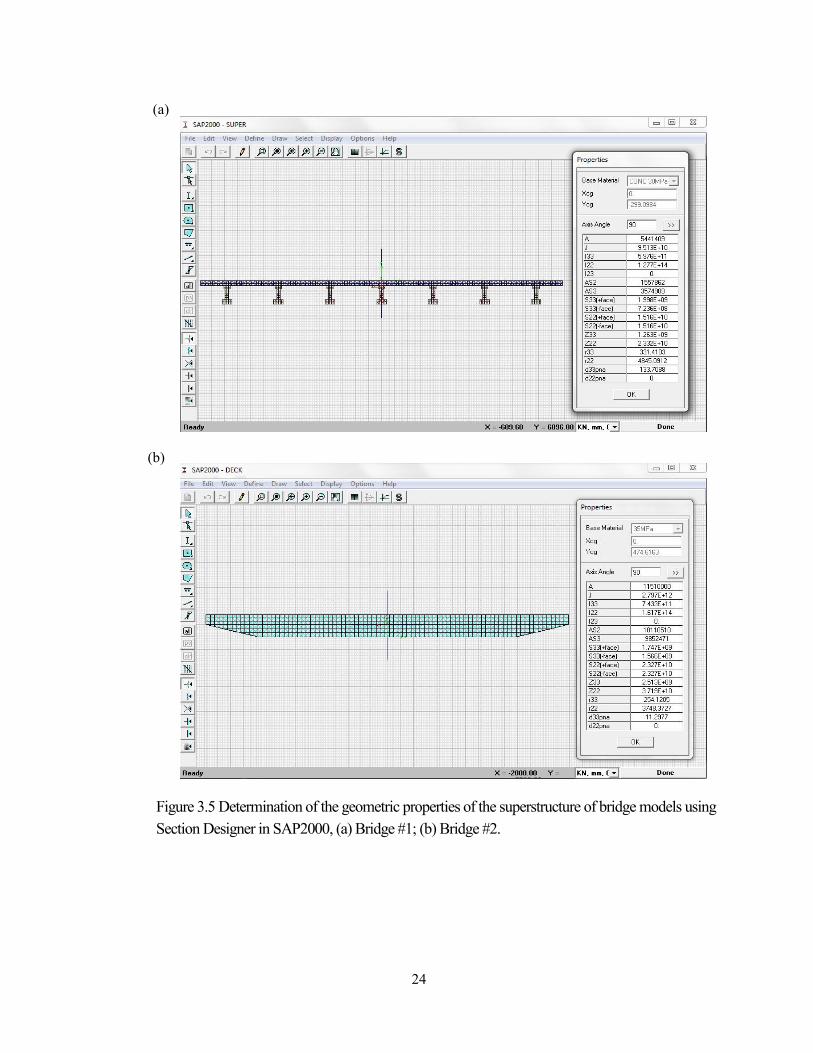
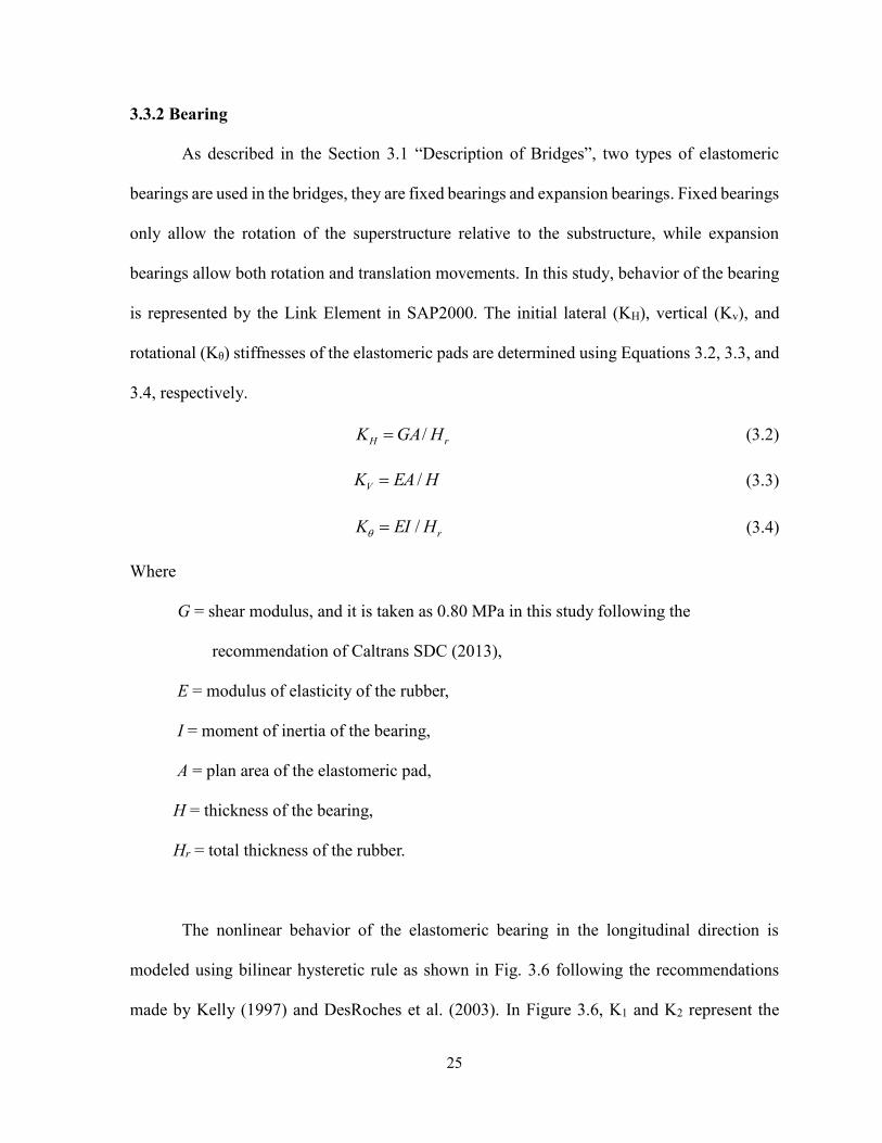
Figure 3.5 Determination of the geometric properties of the superstructure of bridge models

using Section Designer in SAP2000, (a) Bridge #1; (b) Bridge #2…………………………...24

Figure 3.6 Bilinear behavior of elastomeric bearings in the longitudinal direction…………...26

Figure 3.7 Mander Model for confined and unconfined concrete (Adopted from Paulay &

Priestley, 1992)………………………………………………………………………………28

Figure 3.8 Steel stress-strain relationship given in Naumoski et al. (1993)…………………..29

Figure 3.9 Moment-curvature curves of the column section, (a) Bridge #1; (b) Bridge

#2……………………………………………………………………………………………..30

Figure 3.10 Multi-linear Kinematic Plasticity model (Adapted from CSI, 2012) ……………31

Figure 3.11 Detailed modeling of a column bent ……………………………………………31

Figure 3.12 Abutment models, (a) Roller model; (2) Simplified model; (3) Spring model

(Adopted from Aviram et al., 2008a)…………………………………………………………34

Figure 3.13 Mode shapes of the first three modes from the modal analysis, (a) Bridge #1; (b)

Bridge #2……………….…………………………………………………………………….37

Figure 4.1 Design and uniform hazard spectra for Montreal, 5% damping………………….40

Figure 4.2 Seismic hazard deaggregation results for Montreal for probability of exceedance of

10% in 50 years: (a) Sa(0.2s); (b) Sa(1.0s)……………………………………………………42

Figure 4.3 Scaled response spectra of the records based on Sa(T1), Bridge #1, 5%

damping.…………………………..………………………………………………………….45

Figure 5.1 Maximum mean deck displacements according to different superstructure mass:

(a) Bridge #1; (b) Bridge #2…………………………………………………………………..74

viii

Figure 5.2 Maximum mean moments at the base of the column according to different

superstructure mass: (a) Bridge #1; (b) Bridge #2……………………………………………74

Figure 5.3 Maximum mean fixed bearing displacements according to different superstructure

mass: (a) Bridge #1; (b) Bridge #2……………………………………………………………75

Figure 5.4 Maximum mean expansion bearing displacements according to different

superstructure mass: (a) Bridge #1; (b) Bridge #2……………………………………………75

Figure 5.5 Maximum mean column displacements at pier 1 (fixed bearing) according to

different superstructure mass: (a) Bridge #1; (b) Bridge #2…………………………………..76

Figure 5.6 Maximum mean column displacements at pier 2 (expansion bearing) according to


Figure 5.7 Maximum mean column curvature ductilities at pier 1 (fixed bearing) according to


Figure 5.8 Maximum mean column curvature ductilities at pier 2 (expansion bearing)

according to different superstructure mass: (a) Bridge #1; (b) Bridge #2……………………77

Figure 5.9 Moment – curvature relation of an end section of a column using fc’ = 20 MPa, and

fc’ = 40 MPa ………………………………………………………………………………….78

Figure 5.10 Maximum mean deck displacements according to different concrete compressive

strength: (a) Bridge #1; (b) Bridge #2………………………………………………………...79

Figure 5.11 Maximum mean moments at the base of the column according to different concrete

compressive strength: (a) Bridge #1; (b) Bridge #2…………………………………………..79

Figure 5.12 Maximum mean fixed bearing displacements according to different concrete

compressive strength: (a) Bridge #1; (b) Bridge #2………………………………………….80

Figure 5.13 Maximum mean expansion bearing displacements according to different concrete

compressive strength: (a) Bridge #1; (b) Bridge #2…………………………………….…….80


different concrete compressive strength: (a) Bridge #1; (b) Bridge #2………………………..81


different concrete compressive strength: (a) Bridge #1; (b) Bridge #2………………………..81

Figure 5.16 Maximum mean column curvature ductilities at pier 1 (fixed bearing) according

to different concrete compressive strength: (a) Bridge #1; (b) Bridge #2……………………..82


according to different concrete compressive strength: (a) Bridge #1; (b) Bridge #2………….82

ix

Figure 5.18 Maximum mean deck displacements according to different yield strength of the

reinforcing steel: (a) Bridge #1; (b) Bridge #2……………………………………………….83

Figure 5.19 Maximum mean moments at the base of the column according to different yield

strength of the reinforcing steel: (a) Bridge #1; (b) Bridge #2………………………………...83

Figure 5.20 Maximum mean fixed bearing displacements according to different yield strength

of the reinforcing steel: (a) Bridge #1; (b) Bridge #2…………………………………………84

Figure 5.21 Maximum mean expansion bearing displacements according to different yield

strength of the reinforcing steel: (a) Bridge #1; (b) Bridge #2………………………………..84


different yield strength of the reinforcing steel: (a) Bridge #1; (b) Bridge #2………………..85


different yield strength of the reinforcing steel: (a) Bridge #1; (b) Bridge #2…………………85

Figure 5.24 Moment – curvature relation of an end section of a column using fy = 300 MPa,

and fy = 550 MPa …………………………………………………………………………….86


to different yield strength of the reinforcing steel: (a) Bridge #1; (b) Bridge #2……………..87


according to different yield strength of the reinforcing steel: (a) Bridge #1; (b) Bridge #2…...87

Figure 5.27 Maximum mean deck displacements according to different yield displacement of

the bearing: (a) Bridge #1; (b) Bridge #2……………………………………………………88

Figure 5.28 Maximum mean moments at the base of the column according to different yield

displacement of the bearing: (a) Bridge #1; (b) Bridge #2……………………………………88

Figure 5.29 Maximum mean fixed bearing displacements according to different yield


Figure 5.30 Maximum mean expansion bearing displacements according to different yield



different yield displacement of the bearing: (a) Bridge #1; (b) Bridge #2……………………90


different yield displacement of the bearing: (a) Bridge #1; (b) Bridge #2…………………….90


to different yield displacement of the bearing: (a) Bridge #1; (b) Bridge #2………………….91

x


according to different yield displacement of the bearing: (a) Bridge #1; (b) Bridge #2……….91

Figure 5.35 Maximum mean deck displacements according to different post-yield strength of

the bearing: (a) Bridge #1; (b) Bridge #2…………………………………………………….92

Figure 5.36 Maximum mean moments at the base of the column according to different post-

yield strength of the bearing: (a) Bridge #1; (b) Bridge #2……………………………………92

Figure 5.37 Maximum mean fixed bearing displacements according to different post-yield

strength of the bearing: (a) Bridge #1; (b) Bridge #2………………………………………….93

Figure 5.38 Maximum mean expansion bearing displacements according to different post-yield

strength of the bearing: (a) Bridge #1; (b) Bridge #2………………………………………….93


different post-yield strength of the bearing: (a) Bridge #1; (b) Bridge #2…………………….94


different post-yield strength of the bearing: (a) Bridge #1; (b) Bridge #2…………………….94


to different post-yield strength of the bearing: (a) Bridge #1; (b) Bridge #2………………….95


according to different post-yield strength of the bearing: (a) Bridge #1; (b) Bridge #2…….…95

Figure 5.43 Maximum mean deck displacements according to different plastic hinge length:

(a) Bridge #1; (b) Bridge #2…………………………………………………………………..96

Figure 5.44 Maximum mean moments at the base of the column according to different plastic

hinge length: (a) Bridge #1; (b) Bridge #2……………………………………………….…...96

Figure 5.45 Maximum mean fixed bearing displacements according to different plastic hinge

length: (a) Bridge #1; (b) Bridge #2.…………………………………………………………97

Figure 5.46 Maximum mean expansion bearing displacements according to different plastic

hinge length: (a) Bridge #1; (b) Bridge #2……………………………………………………97


different plastic hinge length: (a) Bridge #1; (b) Bridge #2…………………………………..98


different plastic hinge length: (a) Bridge #1; (b) Bridge #2…………………………………...98


to different plastic hinge length: (a) Bridge #1; (b) Bridge #2………………………………..99

xi


according to different plastic hinge length: (a) Bridge #1; (b) Bridge #2……………………..99

Figure 5.51 Maximum mean deck displacements according to different damping: (a) Bridge

#1; (b) Bridge #2……………………………………………………………………………100

Figure 5.52 Maximum mean moments at the base of the column according to different

damping: (a) Bridge #1; (b) Bridge #2………………………………………………………100

Figure 5.53 Maximum mean fixed bearing displacements according to different damping:

(a) Bridge #1; (b) Bridge #2…………………………………………………………………101

Figure 5.54 Maximum mean expansion bearing displacements according to different damping:

(a) Bridge #1; (b) Bridge #2…………………………………………………………………101


different damping: (a) Bridge #1; (b) Bridge #2…………………………………………….102


different damping: (a) Bridge #1; (b) Bridge #2…………………………………………….102


to different damping: (a) Bridge #1; (b) Bridge #2…………………………………………..103


according to different damping: (a) Bridge #1; (b) Bridge #2……………………………….103

1

Chapter 1

Introduction

1.1 Introduction

Bridges are key components in the transportation system of a country. They are

essential for providing a safe flow of traffic along highways and enabling rescue operations

during emergency situations due to natural hazards, such as earthquakes or floods. The

consequences due to failures of highway bridges can be devastating in terms of human

casualties and economical losses. Earthquakes are one of the main natural hazards that have

caused enormous devastations to bridges around the world. Typical examples are the 1989

Loma Prieta and the 1994 Northridge earthquakes in California, the 1995 Kobe earthquake in

Japan, and the 1999 Chi-Chi earthquake in Taiwan, which caused collapse of, or severe damage

to, a large number of bridges. The poor behaviour of the bridges during these earthquakes was

attributed to deficiencies in both the design and construction of the bridges.

The lessons from these and other earthquakes around the world in terms of the seismic

behaviour of existing bridges are very important for Canada. This is because strong

earthquakes can also happen in Canada. The west coast of British Columbia and the Saint

Lawrence valley in eastern Canada, where there are large stocks of bridges, are known to be

seismically active (NRCC, 2010). In addition, many of the existing bridges (especially those

built before 1980) were designed with minimum or no seismic considerations, and are

2

considered vulnerable to seismic motions.

Given the observations from past earthquakes around the world, substantial analytical

and experimental research work related to bridges has been undertaken in Canada and other

countries. The analytical research has been focused primarily on the prediction of the seismic

performance of existing bridges. It includes bridge-specific investigations which are mainly

conducted using deterministic approach, and investigations of bridge portfolios which are

based on probabilistic approach. In both cases, nonlinear time history analyses are extensively

used for the prediction of the seismic responses of the bridges considered. To conduct a

nonlinear time history analysis on a given bridge, analytical (i.e., computational) model of the

bridge and seismic excitations are required. Consequently, the seismic response predictions

depend greatly on both the accuracy of the modeling parameters (or components) considered

in the bridge model, and the characteristics of the seismic excitations used in the nonlinear

analyses.

This research is focussed on the investigation of the effects of the uncertainties of the

modeling parameters on the seismic response of bridges. Specifically, the parameters that will

be investigated include: superstructure mass, concrete compressive strength, yield strength of

the reinforcing steel, yield displacement of the bearing, post-yield stiffness of the bearing,

plastic hinge length, and damping. The uncertainties of the foregoing parameters are inevitable

because of different reasons. For example, the weight of the superstructure might be larger

than the design value due to the forms left inside the girders during construction; the values

used to define the yield displacement and the post-yield stiffness of the bearing are not

provided by the manufacture. For the seismic evaluation of the existing bridges, some of the

modeling parameters mentioned above can be defined based on the construction drawings,

3

such as, the concrete compressive strength and the strength of the steel bars. Others, for

instance, the plastic hinge length, are difficult to define. Furthermore, in most of the studies on

bridge portfolios, the influence of the uncertainties of the foregoing modeling parameters is

included probabilistically by specifying probability distribution functions for the parameter

characteristics, which are normally based on limited information.

1.2 Objective and Scope of the Study

The objective of the study is to determine the effects of the uncertainty of the modeling

parameters on the seismic response of bridges. The parameters that are considered in the

research include:

Superstructure mass,

Concrete compressive strength,

Yield strength of the reinforcing steel,

Yield displacement of the bearing,

Post-yield stiffness of the bearing,

Plastic hinge length, and

Damping.

The response parameters used to examine the effects are,

Deck displacement,

Bearing displacement including both fixed bearing and expansion bearing,

Column displacement,

Column curvature ductility, and

Moment at the base of the column.

4

To achieve the objective of the research, the following tasks are carried out in this study:

Select minimum two existing bridges for the study.

Develop nonlinear models of the selected bridges for use in the time-history

analysis.

Select a set of records appropriate for the seismic analysis of the bridges.

Define the variation of each modeling parameter considered in the study.

Conduct nonlinear time-history analysis by subjecting the bridge model to a

series of seismic excitations to cover the response from elastic to inelastic.

Perform statistical analysis on each response parameter corresponding to the

variation of each modeling parameter.

1.3 Outline of the Thesis

This thesis is organized in 6 chapters. Chapter 2 presents a review of available literature

related to this study. Chapter 3 describes the selection of typical bridges for use in the analysis.

In addition, nonlinear modeling of the selected bridges is presented in detail in this chapter.

Review of seismic hazard in Montreal and selection of appropriate earthquake records for the

time-history analysis of bridges are provided in Chapter 4. The results from the nonlinear time-

history analysis are discussed in Chapter 5 along with the discussion on the effects of the

uncertainty of the modeling parameters on the seismic response of bridges. Finally, Chapter 6

presents the main observations and conclusions resulting from the study. Recommendations

for further research are also included in the chapter.

5

Chapter 2

Literature Review

2.1 Introduction

The server damage to building structures and infrastructure due to 1971 magnitude 6.8

San Fernando Earthquake brought attention to the earthquake engineering community, in

which seismic loads should be considered in the structural design. This earthquake may be

considered as the starting point of the ongoing research and development in the earthquake

safety of structures.

Many of bridges in Canada were built before 1970, and have been in service for more

than 40 years. These bridges were designed with no seismic consideration. The bridges built

between 1970 and 1985 also might be considered deficient for seismic resistance, because the

seismic hazard levels they were designed for were much lower than those based on the current

understanding of the seismic hazard. Given the forgoing considerations, it is wise to evaluate

the seismic performance of the existing bridges in Canada. Two methods are currently used

for such purpose. One is called deterministic approach; the other is called probabilistic

approach. The former is used to conduct investigation on a specific bridge with a given number

of spans, span length, types of bearings, foundation types, and so on. The latter is used to

evaluate the seismic performance of bridge portfolios. In both methods, fragility curves are

commonly used to evaluate the seismic performance of bridges.

6

2.2 Development of Fragility Curves

Fragility curves present the probabilities of a structure or a structure component

reaching and/or exceeding different damage states under a series of ground motions. A simple

expression of the fragility curves is given in Nielson (2005),

Fragility = P [LS | IM = y] (2.1)

where,

P = damage probability

LS = limit state (i.e., a given damage state)

IM = intensity measure for the ground motion (e.g., PGA)

y = a given level of the ground motion (e.g., PGA = 1.0g)

The peak ground acceleration (PGA) of a ground motion was a commonly used IM in the past

for the development of fragility curves of bridges (Nielson, 2005; Pan et al., 2007 and 2010;

Tavares et al., 2012). It was based on the assumption that the period of bridges was generally

quite short. According to HAZUS (FEMA, 2003), the limit state (also known as damage state)

is defined as slight damage, moderate damage, extensive damage, and complete damage.

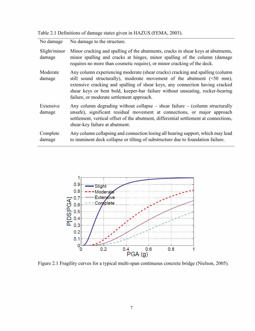
Definitions of damage states mentioned above are given in Table 2.1. For illustration, Figure

2.1 shows fragility curves of a typical multi-span continuous concrete bridge in centre and

southeastern U.S. developed by Nielson (2005).

7

Table 2.1 Definitions of damage states given in HAZUS (FEMA, 2003).

No damage No damage to the structure.

Slight/minor

damage

Minor cracking and spalling of the abutments, cracks in shear keys at abutments,

minor spalling and cracks at hinges, minor spalling of the column (damage

requires no more than cosmetic require), or minor cracking of the deck.

Moderate

damage

Any column experiencing moderate (shear cracks) cracking and spalling (column

still sound structurally), moderate movement of the abutment (<50 mm),

extensive cracking and spalling of shear keys, any connection having cracked

shear keys or bent bold, keeper-bar failure without unseating, rocker-bearing

failure, or moderate settlement approach.

Extensive

damage

Any column degrading without collapse – shear failure – (column structurally

unsafe), significant residual movement at connections, or major approach

settlement, vertical offset of the abutment, differential settlement at connections,

shear-key failure at abutment.

Complete

damage

Any column collapsing and connection losing all bearing support, which may lead

to imminent deck collapse or tilting of substructure due to foundation failure.

Figure 2.1 Fragility curves for a typical multi-span continuous concrete bridge (Nielson, 2005).

8

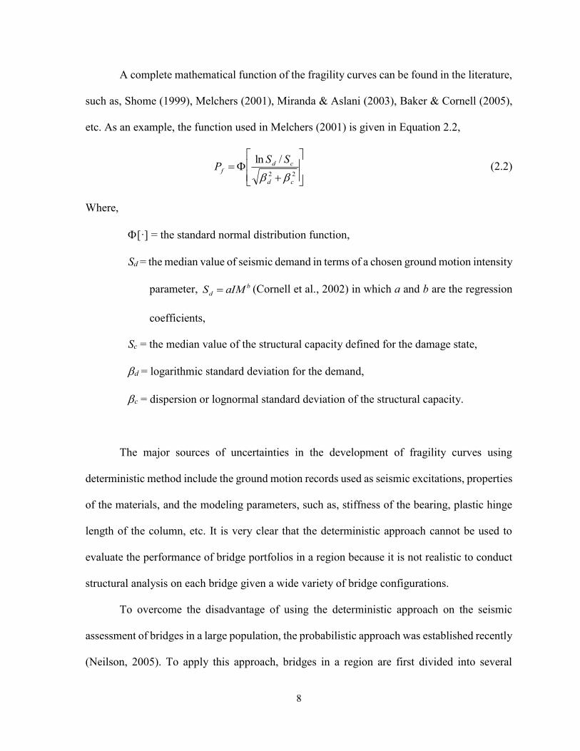
A complete mathematical function of the fragility curves can be found in the literature,

such as, Shome (1999), Melchers (2001), Miranda & Aslani (2003), Baker & Cornell (2005),

etc. As an example, the function used in Melchers (2001) is given in Equation 2.2,

22

/ln

cd

cdf

SSP

(2.2)

Where,

[·] = the standard normal distribution function,

Sd = the median value of seismic demand in terms of a chosen ground motion intensity

parameter, b

d aIMS (Cornell et al., 2002) in which a and b are the regression

coefficients,

Sc = the median value of the structural capacity defined for the damage state,

d = logarithmic standard deviation for the demand,

c = dispersion or lognormal standard deviation of the structural capacity.

The major sources of uncertainties in the development of fragility curves using

deterministic method include the ground motion records used as seismic excitations, properties

of the materials, and the modeling parameters, such as, stiffness of the bearing, plastic hinge

length of the column, etc. It is very clear that the deterministic approach cannot be used to

evaluate the performance of bridge portfolios in a region because it is not realistic to conduct

structural analysis on each bridge given a wide variety of bridge configurations.

To overcome the disadvantage of using the deterministic approach on the seismic

assessment of bridges in a large population, the probabilistic approach was established recently

(Neilson, 2005). To apply this approach, bridges in a region are first divided into several

9

groups. This can be done by considering the following structural characteristics (FEMA, 2003)

(i) span continuity: simply supported, continuous; (ii) number of spans: single- or multiple-

span; (iii) material of construction: concrete, steel; (iv) pier type: multiple-column bents,

single-column bents, and pier walls; (v) abutment type: monolithic, non-monolithic; and (vi)

bearing type: high rocker bearings, low steel bearings and neoprene rubber bearings, such that

bridges in each group are represented by a generic bridge. Then each generic bridge will be

analysed individually based on the typical values of the modeling parameters of the group. The

corresponding fragility curves for each generic bridge can be developed using Eq. 2.2. The

effects of the modeling parameters of each individual bridge, such as, material properties, span

length, thickness of the superstructure, height of the pier, etc. are taken into account

probabilistically by using Monte Carlo method. It can be seen that the probabilistic approach

is not only more complicated than the deterministic method, but also larger uncertainties are

involved in the analysis.

2.3 Review of Previous Studies

A number of parametric studies were conducted in the past to evaluate the effects of

several modeling parameters on the seismic response of bridges in North America. Hwang et

al. (2001) selected a four-span continuous concrete girder bridge in Central United States to

investigate the sensitivity of characteristics of ground motions including the earthquake

magnitude and distance, soil properties, properties of materials (concrete and reinforcing bars),

stiffness of springs used to model the foundation and abutments. The column curvature and

bearing displacement were selected as global response parameters to exam the performance of

bridges. They reported that bearings and columns are very sensitive to earthquake ground

motions.

10

Choi et al. (2004) conducted a study on the effects of the material properties on four

typical bridges in Central and Southeastern United States. The bridges considered in the study

were multi-span simply supported steel girder bridge, multi-span continuous steel girder

bridge, multi-span simply supported pre-stressed concrete girder bridge, and multi-span

continuous pre-stressed concrete girder bridge. They concluded that fixed bearing in multi-

span simply supported steel girder-type bridges is more vulnerable to earthquake than any other

components. They also suggested that all major components including the deck, bearing,

expansion joint, and column should be taken into consideration in the development of fragility

curves.

Nielson (2005) carried out a comprehensive study on development of fragility curves

for nine generic highway bridges. They are (i) multi-span simply supported concrete girder

bridge, (ii) multi-span simply supported concrete box-girder bridge, (iii) multi-span simply

supported slab bridge, (iv) multi-span continuous concrete girder bridge, (v) multi-span

continuous slab bridge, (vi) multi-span simply supported steel girder bridge, (vii) multi-span

continuous steel girder bridge, (viii) single span concrete girder bridge, and (ix) single span

steel girder bridge. A number of uncertainties considered were in the study, such as, bearing

stiffness, coefficient of friction of the bearing, translational and rotational stiffness of the

foundation, direction of seismic excitation, gap width, etc. These uncertainties were considered

in the development of so-called system fragility curves by using Monte-Carlo simulation. The

fragility curves show that steel girder-type bridge is the most vulnerable bridge among all the

nine bridges considered followed by concrete girder-type bridge.

Padgett et al. (2007) performed analysis on multi-span simply supported steel girder

bridge located in Central and Southeastern United States. The purpose of the study was to

11

investigate the effects of the restrainer cables (e.g., yield strength of cable, slack in restrainer

cable, and restrainer cable length), effective stiffness of elastomeric bearings, yield strength of

the steel jackets, and the reinforcing of the shear keys on the behaviour of the bridge. They

found that the direction of the seismic excitation has significant effects on the bridge response

in addition to the bearing stiffness, rotational stiffness of the foundation, and the gap width.

Pekcan et al. (2008) compared analysis results using a detailed finite element model

(FEM) and a simplified beam-stick model on a three-span continuous concrete box-girder

bridge. They reported that the simplified model was better than the FEM if the skew angle of

the bridge is larger than 30 degrees. On the other hand, FEM is preferable for analyzing bridges

with relatively larger skew angle (i.e., skew > 30 degrees) in order to capture higher mode

effects. In addition, they evaluated the bridge performance under different skew angles from

0 to 60 degrees, and concluded that bridge response would increase significantly if the skew

angle is larger than 30 degrees. In general, the structural response changes slightly when the

skew angle is less than 30 degrees. Similarly, Abdel-Mohti (2010) investigated the effect of

skew angle on the seismic response of three reinforced concrete box-girder bridges. However,

the observations are different from those given in Pekcan et al. (2008). Abdel-Mohti (2010)

reported that the bridge deformations and forces increase with the increasing of the skew angle.

Very recently, Pan et al. (2010) conducted a parametric study on a 3-span simply

supported steel girder bridge (it is a generic bridge) in New York using a set of artificial

accelerograms. The parameters considered in the sensitivity analysis were the superstructure

weight, gap size, concrete compressive strength, yield strength of the reinforcement, fraction

coefficient of the expansion bearing. It is necessary to mention that only one response

parameter, i.e., pier curvature ductility, was used to exam the effect of each of the parameters

12

mentioned above on the response of the bridge. They reported that increasing the

superstructure weight would lead to larger curvature ductility. In addition, the pier curvature

ductility decreases with the concrete compressive strength and the yield strength of the

reinforcing bars. They also found that the bridge response is less sensitive to the concrete

compressive stress as compared to the yield strength of the steel.

Few studies on the development of fragility curves of typical highway bridges in

Canada were performed in the last decade. The latest one was conducted by Tavares et al.

(2012), which provides the fragility curves of typical highway bridges in Quebec. Five generic

bridges including the multi-span continuous slab bridge, multi-span continuous concrete girder

bridge, multi-span continuous steel girder bridge, multi-span simply supported concrete girder

bridge, and multi-span simply supported steel girder bridge were considered in the analysis.

This study is very similar to the one carried out by Neilson (2005) in which the uncertainties

of the modeling parameters were taken into account by using Monte-Carlo method. It was

concluded that the stiffness of abutment (both rotational stiffness and translational stiffness)

did not have significant effect on the seismic response of the bridge. Both columns and

elastomeric bearings would sustain severe damage at lower excitation levels which suggests

higher ductility of these two components is required for the design. Another finding given in

Tavares et al. (2012) is the abutment wing wall became fragile at relatively high intensity levels

compared to other components in the bridge.

Some studies focused on investigation the effects of a specific modeling parameter on

the seismic response of bridge. For example, Dicleli & Bruneau (1995) assessed the effect of

number of spans on the response of bridges. Two continuous bridges were used in the study.

One had two spans, and the other had three spans. Dynamic analysis was conducted using only

13

one earthquake record given the earlier stage of research on earthquake engineering. Therefore,

further research is needed by considering other types of bridges (such as simply-supported

bridges) and using more records in the time-history analysis in order to draw a solid conclusion

on the effect of number of spans on the seismic response of bridges.

Aviram et al. (2008a) conducted a comprehensive study on the modeling abutments. In

their study, three types of abutment model were developed, which are designated as roller,

simplified, and spring abutments, respectively. The simple roller abutment model consists of

only single-point constraints (in the vertical direction). The comprehensive spring abutment

model contains discrete representations of the behaviour of backfill, bearing pad, shear key,

and back wall. The simplified model is a compromise between the simple roller model and the

comprehensive spring model. They recommend using a spring model for abutments for short-

span bridges. In most of the research on the seismic assessment of bridges, the stiffness of

abutments was determined based on the recommendations given in Caltrans Seismic Design

Criteria (SDC) (2013). Willson & Tan (1990) also proposed simple formulae for determining

translational and rotational stiffness of abutment in both longitudinal and transverse directions.

Avşar (2009) investigated the effects of the incident angle of seismic motions on the

bridge response and reported that for two-component horizontal excitations, the largest

response of typical (non-curved) bridges is obtained when one component acts in the

longitudinal direction of the bridge and the other component acts in the transverse direction.

In another word, there is no need for assuming a random incident angle of the seismic

excitation, as used in some studies.

14

Chapter 3

Description and Modeling of Bridges

3.1 Introduction

It is known that bridges can be categorized into different groups according to

Span continuity, i.e., simply-supported or continuous,

Number of spans, such as, single-span or multi-span,

Material of construction, e.g., concrete, steel or composite material,

Pier type, such as, wall-type pier or column bent,

Abutment type, i.e., U-type abutment, seat-type abutment, etc.,

Bearing type, e.g., steel bearing, elastomer bearing, etc.

Given the variety of bridges in Canada and for the purpose of this study, it is important to select

bridges that are representative of typical highway bridges for the analysis. Note that the typical

highway bridges are referred to the short- and medium-span bridges, not the long-span bridges

in which the maximum span length is greater than 150 m according to the Canadian Highway

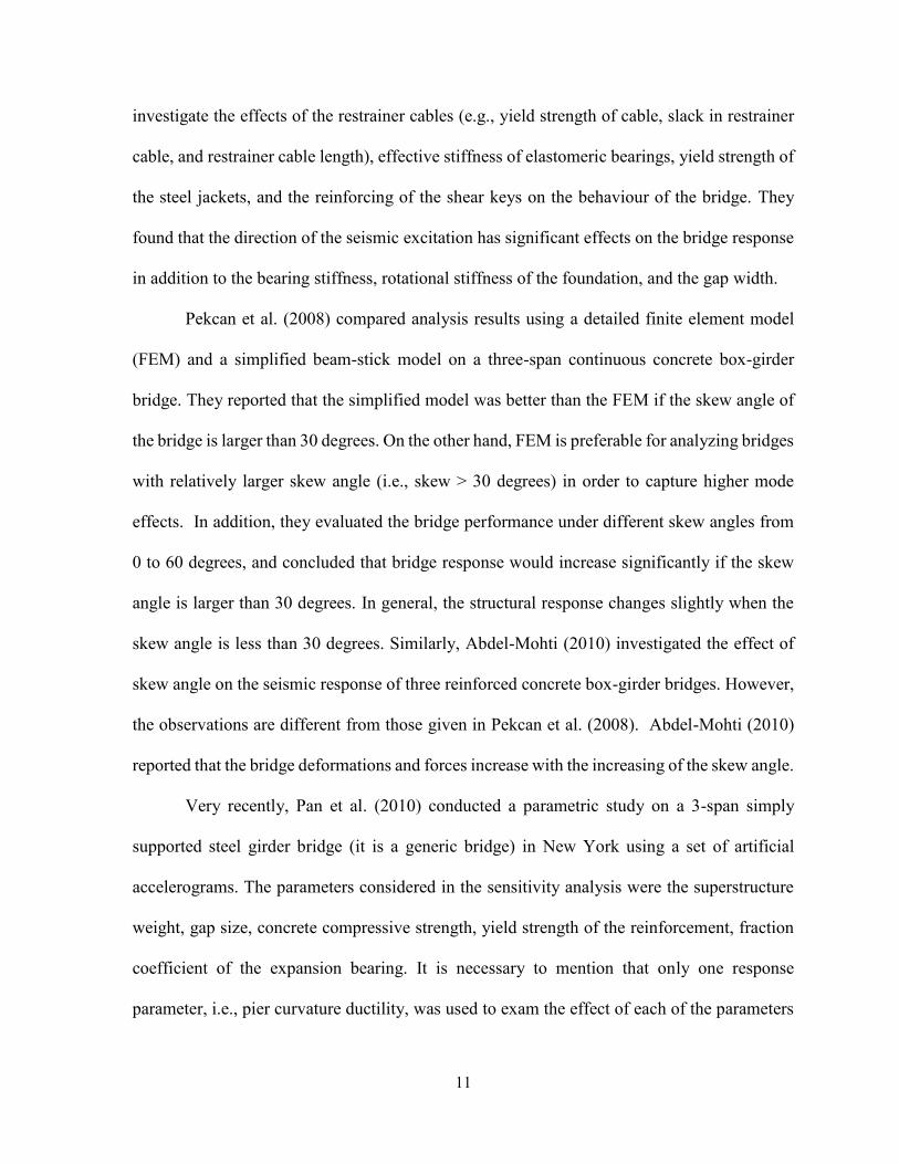
Bridge Design Code (CHBDC, 2006). As reported by Tavares et al. (2012), there are about

2672 multi-span bridges in Quebec in which 25% of them are multi-span simply supported

(MSSS) concrete girder-type bridges, 21% are multi-span continuous (MSC) concrete girder-

type bridges, 11% are multi-span continuous (MSC) slab bridges, 7% are multi-span

continuous (MSC) steel girder-type bridges, and 8% are multi-span simply supported (MSSS)

steel girder-type bridges. The typical cross section of the superstructure of each type of bridges

15

Figure 3.1 Typical bridge classes in Quebec (Adopted from Tavares et al., 2012).

mentioned above is shown in Fig. 3.1. It is necessary to mention that seismic analysis is not

required for one-span simply supported bridges according to CHBDC (2006) due to the fact

that the seismic forces are resisted by abutments which have quite large lateral stiffness.

Consequently, the superstructure of these bridges is not vulnerable to the seismic loads. Tavares

et al. (2012) also found that most of the bridges in Quebec have three spans with seat-type

abutments sitting on shallow foundations. In terms of the column bents, they reported that wall-

type columns, circular columns, and rectangular columns are commonly used. Given these,

two bridges located in Montreal were selected for this study. The first bridge is a three-span

continuous concrete girder-type bridge, and the second one is a three-span continuous concrete

slab bridge. For ease of discussion, these two bridges are referred to as Bridge #1 and Bridge

#2 in the study, respectively. Figures 3.2 and 3.3 show the geometric configurations of two

bridges. Detailed characteristics of the selected bridges are described hereafter.

(a) MSC - MSSS concrete

(b) MSC steel

(c) MSSS steel

(d) MSC slab

16

15000 15500 15000

EXP FIX EXP EXP

I

I

ElevationPier 1 Pier 2

16850

1200

3800

3400

750

16400

5300 5300

I-I section

Column Section

1000

750

16-30M

15M @300 mm Hoop

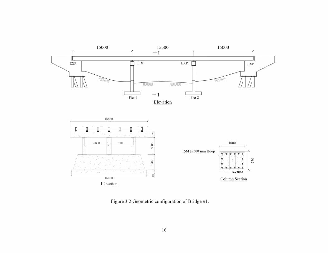
Figure 3.2 Geometric configuration of Bridge #1.

17

I

I

EXP FIX EXP EXP

12600 25200 12600

Elevation

Pier 1 Pier 2

5000

13900

3950 39501300

10500

900

I-I section

Column Section

16-35M Grade 400

1000

15M Spiral@65mm pitch

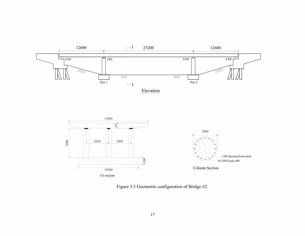
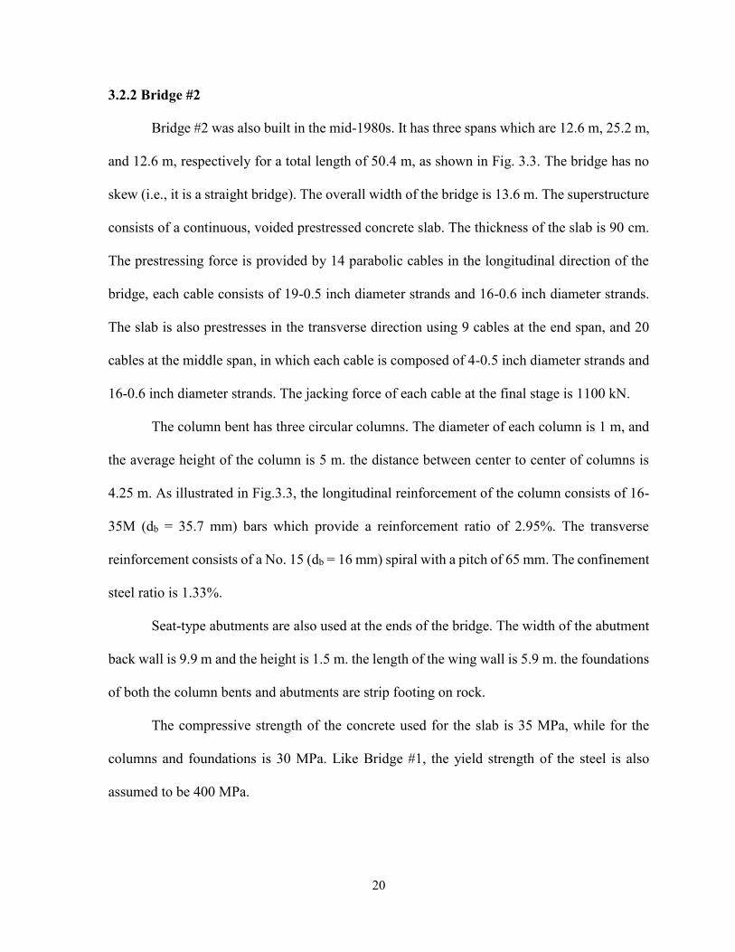
Figure 3.3 Geometric configuration of Bridge #2.

18

3.2 Description of Bridges

3.2.1 Bridge #1

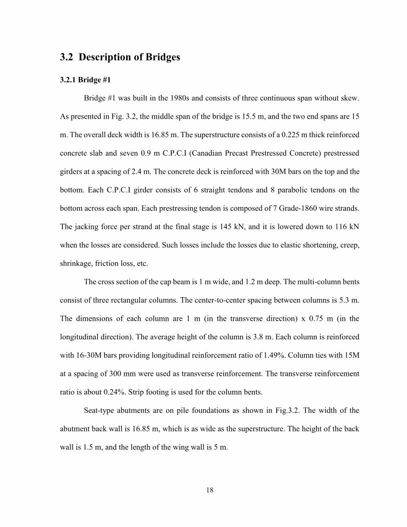
Bridge #1 was built in the 1980s and consists of three continuous span without skew.

As presented in Fig. 3.2, the middle span of the bridge is 15.5 m, and the two end spans are 15

m. The overall deck width is 16.85 m. The superstructure consists of a 0.225 m thick reinforced

concrete slab and seven 0.9 m C.P.C.I (Canadian Precast Prestressed Concrete) prestressed

girders at a spacing of 2.4 m. The concrete deck is reinforced with 30M bars on the top and the

bottom. Each C.P.C.I girder consists of 6 straight tendons and 8 parabolic tendons on the

bottom across each span. Each prestressing tendon is composed of 7 Grade-1860 wire strands.

The jacking force per strand at the final stage is 145 kN, and it is lowered down to 116 kN

when the losses are considered. Such losses include the losses due to elastic shortening, creep,

shrinkage, friction loss, etc.

The cross section of the cap beam is 1 m wide, and 1.2 m deep. The multi-column bents

consist of three rectangular columns. The center-to-center spacing between columns is 5.3 m.

The dimensions of each column are 1 m (in the transverse direction) x 0.75 m (in the

longitudinal direction). The average height of the column is 3.8 m. Each column is reinforced

with 16-30M bars providing longitudinal reinforcement ratio of 1.49%. Column ties with 15M

at a spacing of 300 mm were used as transverse reinforcement. The transverse reinforcement

ratio is about 0.24%. Strip footing is used for the column bents.

Seat-type abutments are on pile foundations as shown in Fig.3.2. The width of the

abutment back wall is 16.85 m, which is as wide as the superstructure. The height of the back

wall is 1.5 m, and the length of the wing wall is 5 m.

19

For the deck and columns, the compressive strength of concrete is 30 MPa. For the

girders, it is 35 MPa whereas it is 20 MPa for the cap beam. No information could be obtained

from the original bridge drawings on the stress of the reinforcing steel used in the structure.

Therefore, the yield strength of the reinforcement is assumed to be 400 MPa.

As shown in Fig. 3.2, expansion bearings, which allow both translation and rotation,

are used on the abutments and pier 2. Fixed bearings, which allow translation only (i.e., not

rotation), are used on the pier 1. Due to the lack of information on the type of bearings used in

the bridge, elastomeric bearings are considered given their good performance against the

seismic loads (Pan et al., 2010; Fu, 2013), and they were designed according to CHBDC

(2006). The requirements specified in AASHTO (2014) are also used to finalize the bearing

design. More specifically, the bearings designed satisfy the following requirements:

Maximum instantaneous compressive deflection,

Bearing maximum rotation,

Bearing combined compression and rotation including uplift requirement and

shear deformation requirement,

Bearing stability.

Rectangular elastomeric bearing (450 mm x 350 mm x 100 mm) is used on the bottom

of each girder at the abutments and piers. Each bearing consists of 4 layers of the steel plate

and 6 layers of elastomer. The thickness of the steel plate is 2 mm, and the total thickness of

the elastomer is 80 mm. It is necessary to mention that both fixed bearings and expansion

bearings have the same size. As illustrated in Figs. 3.2 and 3.3, the fixed bearing and expansion

bearing are drawn as triangle and circular shapes, respectively.

20

3.2.2 Bridge #2

Bridge #2 was also built in the mid-1980s. It has three spans which are 12.6 m, 25.2 m,

and 12.6 m, respectively for a total length of 50.4 m, as shown in Fig. 3.3. The bridge has no

skew (i.e., it is a straight bridge). The overall width of the bridge is 13.6 m. The superstructure

consists of a continuous, voided prestressed concrete slab. The thickness of the slab is 90 cm.

The prestressing force is provided by 14 parabolic cables in the longitudinal direction of the

bridge, each cable consists of 19-0.5 inch diameter strands and 16-0.6 inch diameter strands.

The slab is also prestresses in the transverse direction using 9 cables at the end span, and 20

cables at the middle span, in which each cable is composed of 4-0.5 inch diameter strands and

16-0.6 inch diameter strands. The jacking force of each cable at the final stage is 1100 kN.

The column bent has three circular columns. The diameter of each column is 1 m, and

the average height of the column is 5 m. the distance between center to center of columns is

4.25 m. As illustrated in Fig.3.3, the longitudinal reinforcement of the column consists of 16-

35M (db = 35.7 mm) bars which provide a reinforcement ratio of 2.95%. The transverse

reinforcement consists of a No. 15 (db = 16 mm) spiral with a pitch of 65 mm. The confinement

steel ratio is 1.33%.

Seat-type abutments are also used at the ends of the bridge. The width of the abutment

back wall is 9.9 m and the height is 1.5 m. the length of the wing wall is 5.9 m. the foundations

of both the column bents and abutments are strip footing on rock.

The compressive strength of the concrete used for the slab is 35 MPa, while for the

columns and foundations is 30 MPa. Like Bridge #1, the yield strength of the steel is also

assumed to be 400 MPa.

21

Rectangular elastomeric bearings with 600 mm x 600 mm x 130 mm are chosen to

place on the top of each column at the abutments and piers. The bearing consists of 5 layers of

the steel plate with the thickness of 2 mm each layer. The total thickness of the elastomer is 40

mm. Fixed bearings are used on the Pier 1, and expansion bearings are used on the abutments

and Pier 2 (Fig. 3.3). The fixed bearings and the expansion bearings also have the same size

like Bridge #1.

3.3 Modeling of Bridges

In this study, three-dimensional finite element models were developed by using the

structural analysis software SAP2000 (CSI, 2012) for the purpose of analyses. SAP2000 has

been used in a number of studies on the evaluation of bridges subjected to seismic loads

(Shafiei-Tehrany, 2008; Pan et al., 2010; Waller, 2010; etc.). The advantage of SAP2000 is a

number of elements (e.g., link element) are available which can be used to model the

nonlinearity of different components of a bridge system including bearings and plastic hinges

during seismic excitations. It is necessary to mention that another program OpenSees

(McKenna & Feneves, 2005) can also be used for the nonlinear analysis of bridges. However,

a study conducted by Aviram et al. (2008a) showed that these two programs provide very

similar results. SAP2000 was selected for this study due to its simplicity in modeling and less

time-consuming in the analysis compared with OpenSees.

3.3.1 Superstructure

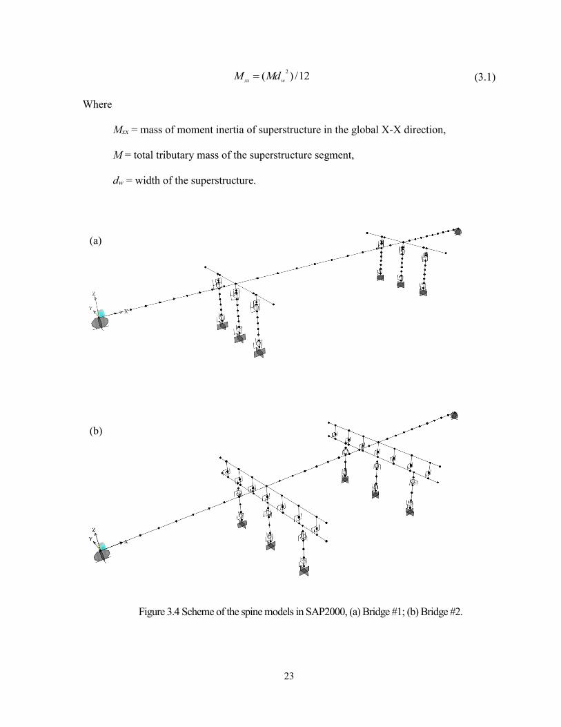
A spine model shown in Fig. 3.4 was used to model the superstructure for each bridge

considered in this study. According to the capacity design method specified in AASHTO (2014)

and CHBDC (2006), the superstructure of the bridge system should remain elastic during

22

earthquake events. Therefore, the superstructure was modeled using elastic beam elements

located along the centroid of the superstructure. Each span of the bridge is discretized into 10

equal segments in order to achieve higher accuracy of the results. It is necessary to mention

that a minimum number of four elements per span are required for modeling the superstructure

according to ATC-32 (1996). The properties of superstructure (i.e., the cross-sectional area,

moment inertia, shear area, torsional constant, etc.) of each bridge were defined using “Section

Designer” which is an integrated utility built into SAP2000. For illustration, Figures 3.5a and

3.5b show the typical geometric properties of the Bridge #1 and Bridge #2 considered in this

study, respectively. It is known that both the flexural moment of inertia and the torsional

moment of inertia have significant effects on the bridge response. In this study, a factor of 0.75

was used to reduce the moment of inertia of the deck section, and no reduction factor was

applied to the girder sections as recommended by Caltrans SDC (2013). Reduction of the

torsional moment of inertia was not considered given the regularity of the bridge according to

Caltrans SDC (2013).

The total mass of the bridge was lumped to the nodes of the superstructure. It is

necessary to mention that the weight of the cap beams (for Bridge #1) and the half weight of

the column bents were lumped to the nodes of the superstructure (i.e., nodes in the longitudinal

direction X-X, Fig. 3.4) at the Piers 1 and 2. Note that the translational mass lumped to each

node can be calculated by the program itself, and it is assigned to each of the three global axes

(X, Y, and Z as shown in Fig. 3.4). However, the rotational mass (i.e., the rotational mass

moment of inertia) cannot be calculated by the program itself, i.e., it must be calculated

manually. The rotational mass moment of inertia of the superstructure can be determined using

Equation 3.1,

23

12/)(2

wxxMdM (3.1)

Where

Mxx = mass of moment inertia of superstructure in the global X-X direction,

M = total tributary mass of the superstructure segment,

dw = width of the superstructure.

(a)

(b)

Figure 3.4 Scheme of the spine models in SAP2000, (a) Bridge #1; (b) Bridge #2.

24

Figure 3.5 Determination of the geometric properties of the superstructure of bridge models using

Section Designer in SAP2000, (a) Bridge #1; (b) Bridge #2.

(a)

(b)

25

3.3.2 Bearing

As described in the Section 3.1 “Description of Bridges”, two types of elastomeric

bearings are used in the bridges, they are fixed bearings and expansion bearings. Fixed bearings

only allow the rotation of the superstructure relative to the substructure, while expansion

bearings allow both rotation and translation movements. In this study, behavior of the bearing

is represented by the Link Element in SAP2000. The initial lateral (KH), vertical (Kv), and

rotational (Kθ) stiffnesses of the elastomeric pads are determined using Equations 3.2, 3.3, and

3.4, respectively.

rH HGAK / (3.2)

HEAKV / (3.3)

rHEIK / (3.4)

Where

G = shear modulus, and it is taken as 0.80 MPa in this study following the

recommendation of Caltrans SDC (2013),

E = modulus of elasticity of the rubber,

I = moment of inertia of the bearing,

A = plan area of the elastomeric pad,

H = thickness of the bearing,

Hr = total thickness of the rubber.

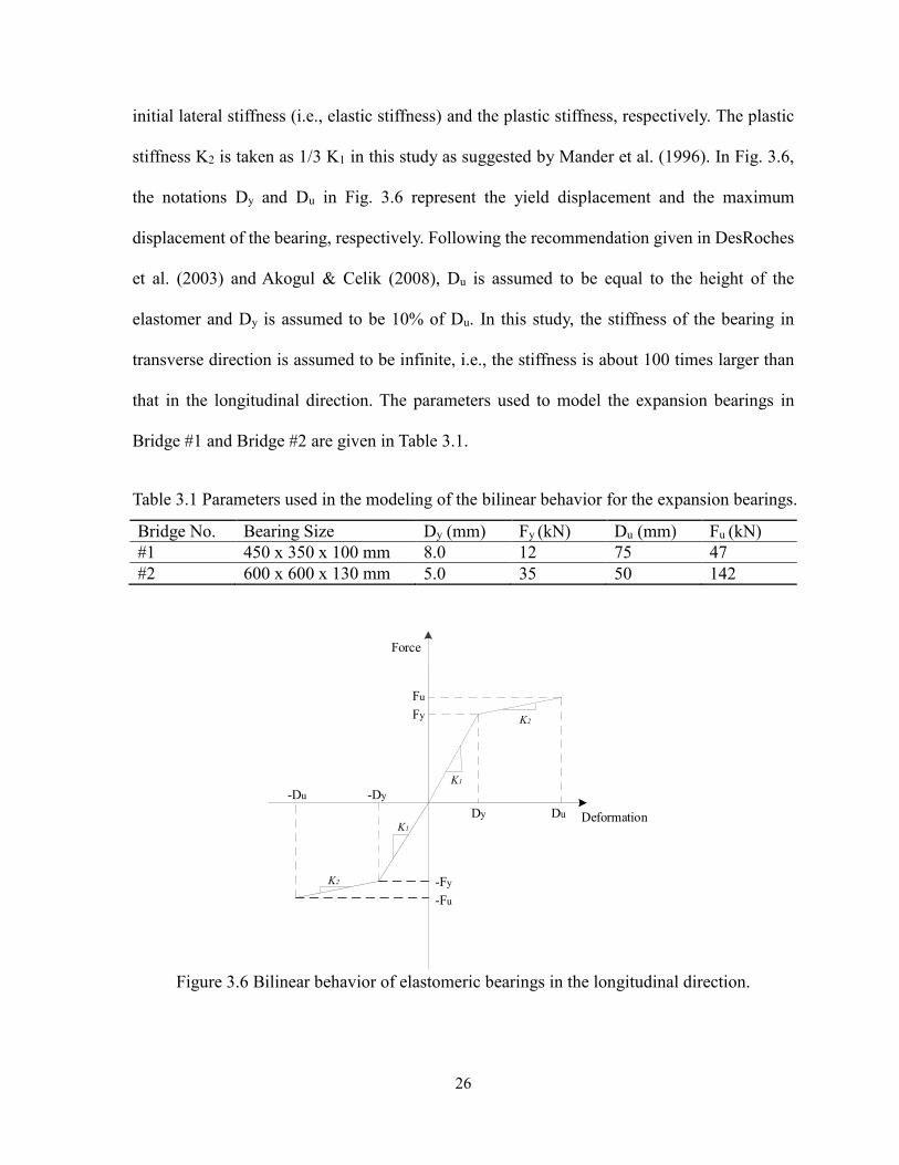
The nonlinear behavior of the elastomeric bearing in the longitudinal direction is

modeled using bilinear hysteretic rule as shown in Fig. 3.6 following the recommendations

made by Kelly (1997) and DesRoches et al. (2003). In Figure 3.6, K1 and K2 represent the

26

initial lateral stiffness (i.e., elastic stiffness) and the plastic stiffness, respectively. The plastic

stiffness K2 is taken as 1/3 K1 in this study as suggested by Mander et al. (1996). In Fig. 3.6,

the notations Dy and Du in Fig. 3.6 represent the yield displacement and the maximum

displacement of the bearing, respectively. Following the recommendation given in DesRoches

et al. (2003) and Akogul & Celik (2008), Du is assumed to be equal to the height of the

elastomer and Dy is assumed to be 10% of Du. In this study, the stiffness of the bearing in

transverse direction is assumed to be infinite, i.e., the stiffness is about 100 times larger than

that in the longitudinal direction. The parameters used to model the expansion bearings in

Bridge #1 and Bridge #2 are given in Table 3.1.

Table 3.1 Parameters used in the modeling of the bilinear behavior for the expansion bearings.

Bridge No. Bearing Size Dy (mm) Fy (kN) Du (mm) Fu (kN)

#1 450 x 350 x 100 mm 8.0 12 75 47

#2 600 x 600 x 130 mm 5.0 35 50 142

Force

Deformation

K1

K2

Dy

-Dy

K1

K2

Du

-Du

Fu

Fy

-Fu

-Fy

Figure 3.6 Bilinear behavior of elastomeric bearings in the longitudinal direction.

27

3.3.3 Columns and Cap Beams

It is expected that plastic hinges would form on the bottom and/or top of a column

during larger earthquake events (Paulay & Priestley, 1992). In this study, plastic hinges were

assumed on both the bottom and top of the column in accordance with the seismic provisions

of the New Zealand Code (TNZ, 2003). It should be noted that the current edition of the

CHBDC (2006) does not specify the location of the plastic hinge. The plastic hinge zones are

modeled with nonlinear elements while the rest part of the column is modeled by elastic

elements. The detail description on the modeling of the columns and cap beams is given

hereafter.

3.3.3.1 Modeling the plastic hinge zone

Plastic Hinge Length

According to CHBDC (2006), the plastic hinge length Lp shall be taken as the

maximum value of (i) the maximum cross-sectional dimension of the column, (ii) one-sixth of

the clear height of the column, and (iii) 450 mm. Therefore, the plastic hinge length Lp of the

columns for Bridge #1 is considered as 1 m, and for Bridge #2 is 0.72 m (see Fig. 3.2 and 3.3),

respectively. In this study, the plastic hinge length of the column was also determined using

the formula provided by Caltrans SDC (2013) which is expressed in Eq. 3.5.

blyeblyepdfdfLL 044.0022.008.0 (3.5)

Where

L = height of column, in mm

fye = expected yield strength of the steel bar, in MPa

dbl = diameter of a longitudinal rebar, in mm

28

Using Eq. 3.5, it was found that the plastic hinge length of the column of Bridge #1

was 720 mm while it was 610 mm for Bridge #2. Based on the calculation following the

specifications of CHBDC and Caltrans, plastic hinge length of the column of 1.0 m was used

in the model of Bridge #1, and 0.72 m was used in the model of Bridge #2.

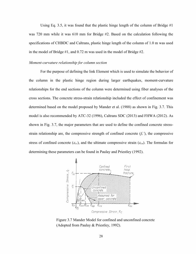
Moment-curvature relationship for column section

For the purpose of defining the link Element which is used to simulate the behavior of

the column in the plastic hinge region during larger earthquakes, moment-curvature

relationships for the end sections of the column were determined using fiber analyses of the

cross sections. The concrete stress-strain relationship included the effect of confinement was

determined based on the model proposed by Mander et al. (1988) as shown in Fig. 3.7. This

model is also recommended by ATC-32 (1996), Caltrans SDC (2013) and FHWA (2012). As

shown in Fig. 3.7, the major parameters that are used to define the confined concrete stress-

strain relationship are, the compressive strength of confined concrete (fc’), the compressive

stress of confined concrete (cc), and the ultimate compressive strain (cu). The formulas for

determining these parameters can be found in Paulay and Priestley (1992).

Figure 3.7 Mander Model for confined and unconfined concrete

(Adopted from Paulay & Priestley, 1992).

29

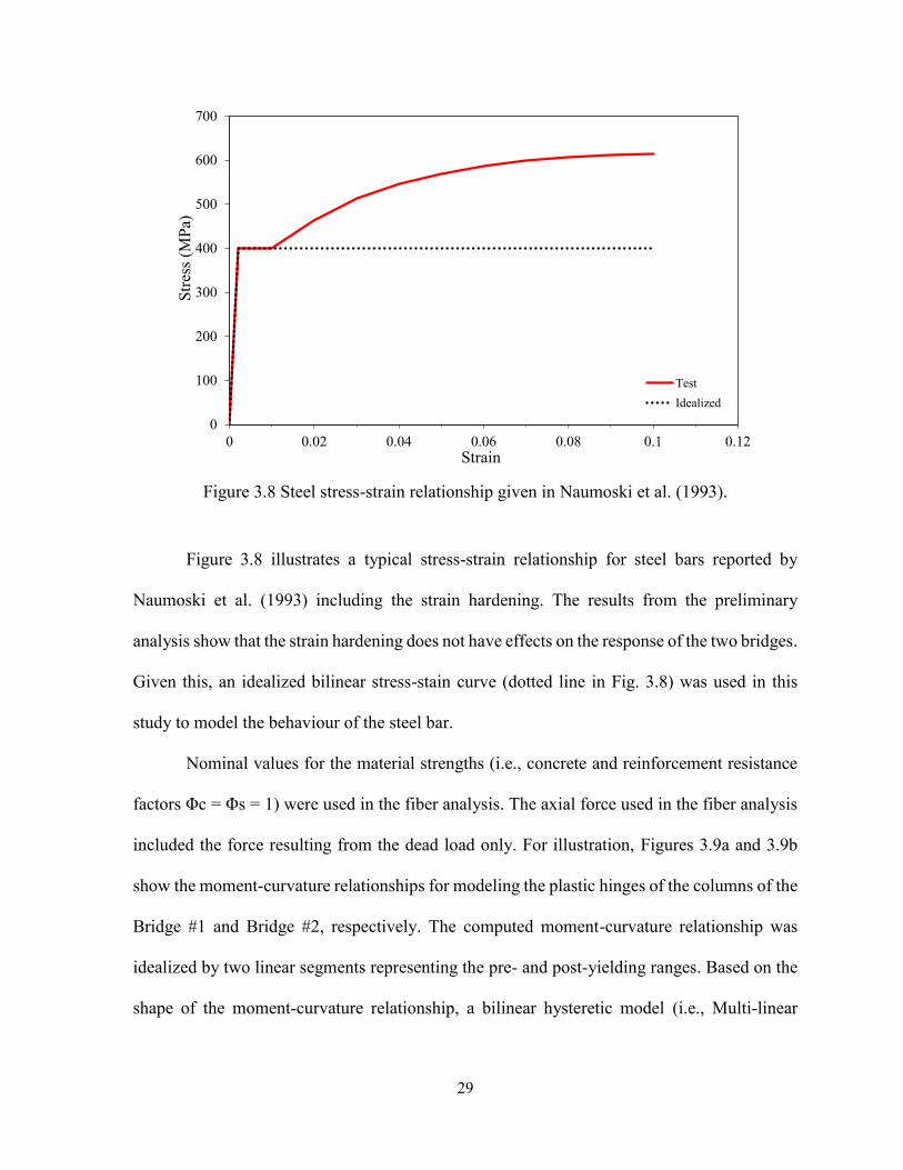
Figure 3.8 Steel stress-strain relationship given in Naumoski et al. (1993).

Figure 3.8 illustrates a typical stress-strain relationship for steel bars reported by

Naumoski et al. (1993) including the strain hardening. The results from the preliminary

analysis show that the strain hardening does not have effects on the response of the two bridges.

Given this, an idealized bilinear stress-stain curve (dotted line in Fig. 3.8) was used in this

study to model the behaviour of the steel bar.

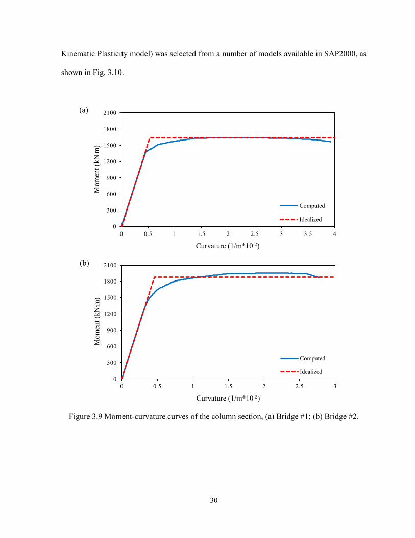
Nominal values for the material strengths (i.e., concrete and reinforcement resistance

factors Φc = Φs = 1) were used in the fiber analysis. The axial force used in the fiber analysis

included the force resulting from the dead load only. For illustration, Figures 3.9a and 3.9b

show the moment-curvature relationships for modeling the plastic hinges of the columns of the

Bridge #1 and Bridge #2, respectively. The computed moment-curvature relationship was

idealized by two linear segments representing the pre- and post-yielding ranges. Based on the

shape of the moment-curvature relationship, a bilinear hysteretic model (i.e., Multi-linear

0

100

200

300

400

500

600

700

0 0.02 0.04 0.06 0.08 0.1 0.12

Str

ess

(MP

a)

Strain

Test

Idealized

30

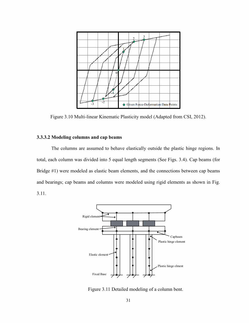
Kinematic Plasticity model) was selected from a number of models available in SAP2000, as

shown in Fig. 3.10.

Figure 3.9 Moment-curvature curves of the column section, (a) Bridge #1; (b) Bridge #2.

0

300

600

900

1200

1500

1800

2100

0 0.5 1 1.5 2 2.5 3 3.5 4

Mom

ent

(kN

. m)

Curvature (1/m*10-2)

Computed

Idealized

0

300

600

900

1200

1500

1800

2100

0 0.5 1 1.5 2 2.5 3

Mom

ent

(kN

. m)

Curvature (1/m*10-2)

Computed

Idealized

(a)

(b)

31

Figure 3.10 Multi-linear Kinematic Plasticity model (Adapted from CSI, 2012).

3.3.3.2 Modeling columns and cap beams

The columns are assumed to behave elastically outside the plastic hinge regions. In

total, each column was divided into 5 equal length segments (See Figs. 3.4). Cap beams (for

Bridge #1) were modeled as elastic beam elements, and the connections between cap beams

and bearings; cap beams and columns were modeled using rigid elements as shown in Fig.

3.11.

Figure 3.11 Detailed modeling of a column bent.

Plastic hinge element

Plastic hinge elment

Elastic element

Bearing element

Rigid element

Capbeam

Fixed Base

32

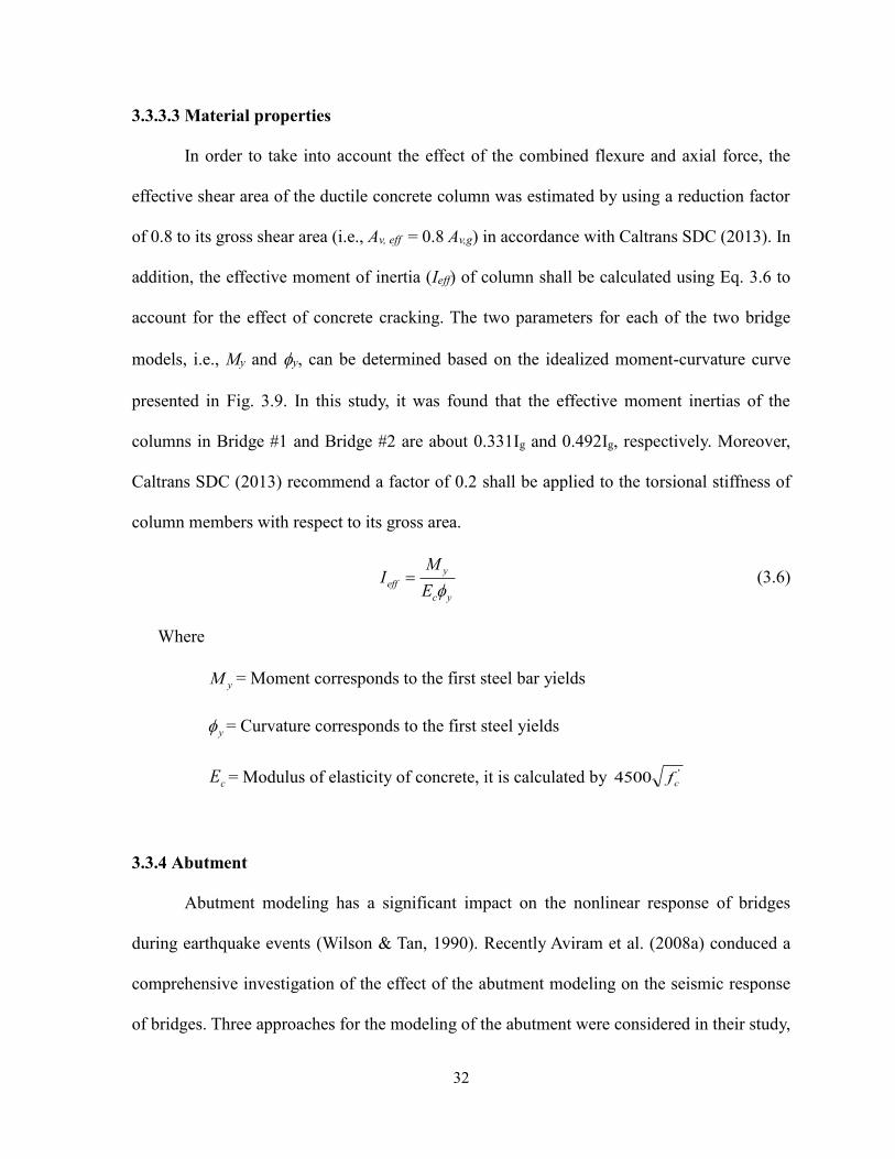
3.3.3.3 Material properties

In order to take into account the effect of the combined flexure and axial force, the

effective shear area of the ductile concrete column was estimated by using a reduction factor

of 0.8 to its gross shear area (i.e., Av, eff = 0.8 Av,g) in accordance with Caltrans SDC (2013). In

addition, the effective moment of inertia (Ieff) of column shall be calculated using Eq. 3.6 to

account for the effect of concrete cracking. The two parameters for each of the two bridge

models, i.e., My and y, can be determined based on the idealized moment-curvature curve

presented in Fig. 3.9. In this study, it was found that the effective moment inertias of the

columns in Bridge #1 and Bridge #2 are about 0.331Ig and 0.492Ig, respectively. Moreover,

Caltrans SDC (2013) recommend a factor of 0.2 shall be applied to the torsional stiffness of

column members with respect to its gross area.

yc

y

effE

MI

(3.6)

Where

yM = Moment corresponds to the first steel bar yields

y = Curvature corresponds to the first steel yields

cE = Modulus of elasticity of concrete, it is calculated by '4500 cf

3.3.4 Abutment

Abutment modeling has a significant impact on the nonlinear response of bridges

during earthquake events (Wilson & Tan, 1990). Recently Aviram et al. (2008a) conduced a

comprehensive investigation of the effect of the abutment modeling on the seismic response

of bridges. Three approaches for the modeling of the abutment were considered in their study,

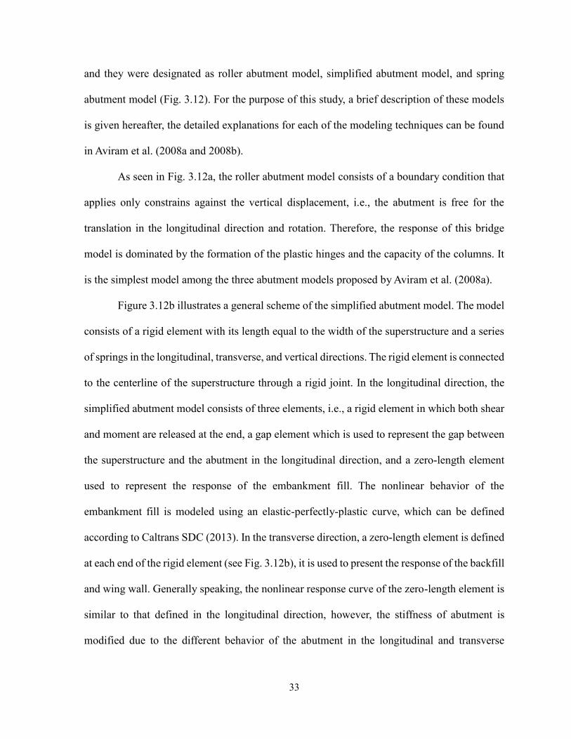
33

and they were designated as roller abutment model, simplified abutment model, and spring

abutment model (Fig. 3.12). For the purpose of this study, a brief description of these models

is given hereafter, the detailed explanations for each of the modeling techniques can be found

in Aviram et al. (2008a and 2008b).

As seen in Fig. 3.12a, the roller abutment model consists of a boundary condition that

applies only constrains against the vertical displacement, i.e., the abutment is free for the

translation in the longitudinal direction and rotation. Therefore, the response of this bridge

model is dominated by the formation of the plastic hinges and the capacity of the columns. It

is the simplest model among the three abutment models proposed by Aviram et al. (2008a).

Figure 3.12b illustrates a general scheme of the simplified abutment model. The model

consists of a rigid element with its length equal to the width of the superstructure and a series

of springs in the longitudinal, transverse, and vertical directions. The rigid element is connected

to the centerline of the superstructure through a rigid joint. In the longitudinal direction, the

simplified abutment model consists of three elements, i.e., a rigid element in which both shear

and moment are released at the end, a gap element which is used to represent the gap between

the superstructure and the abutment in the longitudinal direction, and a zero-length element

used to represent the response of the embankment fill. The nonlinear behavior of the

embankment fill is modeled using an elastic-perfectly-plastic curve, which can be defined

according to Caltrans SDC (2013). In the transverse direction, a zero-length element is defined

at each end of the rigid element (see Fig. 3.12b), it is used to present the response of the backfill

and wing wall. Generally speaking, the nonlinear response curve of the zero-length element is

similar to that defined in the longitudinal direction, however, the stiffness of abutment is

modified due to the different behavior of the abutment in the longitudinal and transverse

34

directions. In the vertical direction, elastic spring is defined at each end of the rigid element.

The stiffness of the spring is equal to the stiffness of the total bearing pads.

Figure 3.12 Abutment models, (a) Roller model; (2) Simplified model;

(3) Spring model (Adopted from Aviram et al., 2008a).

(a)

(b)

(c)

35

The spring abutment model is an improved model based on the simplified abutment

model, and a general scheme of the model is presented in Fig. 3.12c. The spring model

considers the nonlinear response of the abutment in the longitudinal, transverse, and vertical

directions while the simplified abutment model considers the nonlinear response of the

abutment in the longitudinal and transverse directions (i.e., the simplified model assumes the

response of the abutment in the vertical direction is linear). As shown in Fig. 3.12c, the

responses of both bearing pads and embankments are considered in the modeling.

Aviram et al. (2008a) used six different types of bridges for the investigation.

Nonlinear time-history analyses were conducted on each bridge by using the three abutment

models described above. They concluded that the roller model provided relatively conservative

results while simplified model and the spring model provided very similar longitudinal

displacement. The dominant periods of the bridge obtained from these three abutment models

are relatively close except that the first mode period of the bridge from the spring model is

significantly smaller than that from the roller model and the simplified model. Given these and

the objective of this study (i.e., selection appropriate records for use for the nonlinear time-

history analysis of bridges), the roller abutment model was selected due to its lowest model

complexity.

3.4 Dynamic Characteristics of the Bridge Models

In this study, modal analysis was conducted first on the bridge models in order to

understand the dynamic characteristics of the two bridges. In total, 12 modes were considered

in the modal analysis for each bridge. Rayleigh damping of 5% of critical was assigned to all

the 12 modes of each bridge model. The damping was specified to be proportional to the initial

stiffness of the models.

36

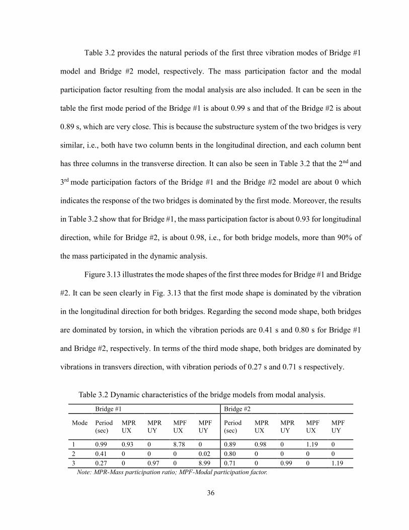
Table 3.2 provides the natural periods of the first three vibration modes of Bridge #1

model and Bridge #2 model, respectively. The mass participation factor and the modal

participation factor resulting from the modal analysis are also included. It can be seen in the

table the first mode period of the Bridge #1 is about 0.99 s and that of the Bridge #2 is about

0.89 s, which are very close. This is because the substructure system of the two bridges is very

similar, i.e., both have two column bents in the longitudinal direction, and each column bent

has three columns in the transverse direction. It can also be seen in Table 3.2 that the 2nd and

3rd mode participation factors of the Bridge #1 and the Bridge #2 model are about 0 which

indicates the response of the two bridges is dominated by the first mode. Moreover, the results

in Table 3.2 show that for Bridge #1, the mass participation factor is about 0.93 for longitudinal

direction, while for Bridge #2, is about 0.98, i.e., for both bridge models, more than 90% of

the mass participated in the dynamic analysis.

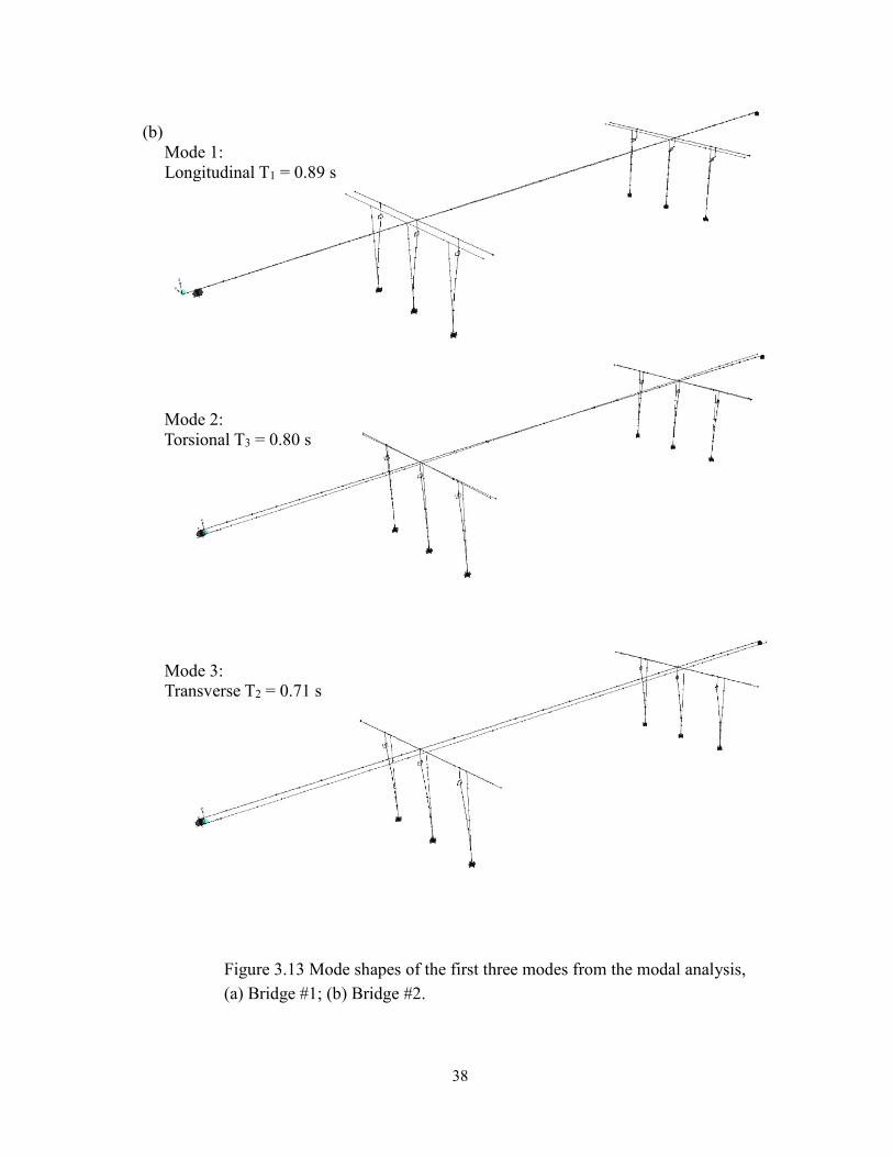
Figure 3.13 illustrates the mode shapes of the first three modes for Bridge #1 and Bridge

#2. It can be seen clearly in Fig. 3.13 that the first mode shape is dominated by the vibration

in the longitudinal direction for both bridges. Regarding the second mode shape, both bridges

are dominated by torsion, in which the vibration periods are 0.41 s and 0.80 s for Bridge #1

and Bridge #2, respectively. In terms of the third mode shape, both bridges are dominated by

vibrations in transvers direction, with vibration periods of 0.27 s and 0.71 s respectively.

Table 3.2 Dynamic characteristics of the bridge models from modal analysis.

Bridge #1 Bridge #2

Mode

Period

(sec)

MPR

UX

MPR

UY

MPF

UX

MPF

UY

Period

(sec)

MPR

UX

MPR

UY

MPF

UX

MPF

UY

1 0.99 0.93 0 8.78 0 0.89 0.98 0 1.19 0

2 0.41 0 0 0 0.02 0.80 0 0 0 0

3 0.27 0 0.97 0 8.99 0.71 0 0.99 0 1.19

Note: MPR-Mass participation ratio; MPF-Modal participation factor.

37

Mode 3:

Transverse T3 = 0.27 s

Model 2:

Torsional T2 = 0.41 s

(a)

Mode 1:

Longitudinal T1 = 0.99 s

38

Figure 3.13 Mode shapes of the first three modes from the modal analysis,

(a) Bridge #1; (b) Bridge #2.

Mode 3:

Transverse T2 = 0.71 s

Mode 2:

Torsional T3 = 0.80 s

(b)

Mode 1:

Longitudinal T1 = 0.89 s

39

Chapter 4

Selection of Earthquake Records

4.1 Seismic Hazard for Montreal

With improvement on our knowledge, currently the seismic hazard for a given site is

represented by a uniform hazard spectrum rather than by the peak ground acceleration or peak

ground velocity which was used about 20 years ago. A uniform hazard spectrum represents an

acceleration spectrum with spectral ordinates having the same probability of exceedance.

Uniform hazard spectra can be computed for different probabilities (e.g., 2% in 50 years, 10%

in 50 years, etc.) and different confidence levels. Two typical confidence levels used to define

uniform hazard spectra are 50% and 84% which represent the confidence in percentage that

the spectral values will not be exceeded for the specified probability. Figure 4.1 shows the 50%

and 84% levels uniform hazard spectrum (UHS) for the probability of exceedance of 10% in

50 years (i.e., annual probability of exceedance of 0.002) for 5% damping for soil class C while

the spectral values were provided by Geological Survey of Canada. The soil class C is referred

to the soil with the shear wave velocity between 360 m/s and 750 m/s according to the National

Building Code of Canada (NRCC 2010). It is necessary to mention that the probability of

exceedance of 10% in 50 years is the design earthquake level specified in CHBDC (2006).

The seismic response coefficient (i.e., seismic design spectrum) for Montreal was

determined using Equation (4.1) in accordance with CHBDC (2006),

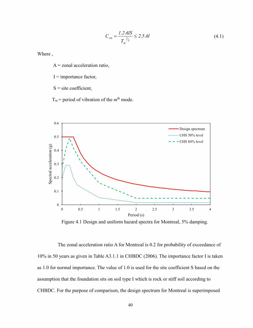
40

(4.1)

Where ,

A = zonal acceleration ratio,

I = importance factor,

S = site coefficient,

Tm = period of vibration of the mth mode.

Figure 4.1 Design and uniform hazard spectra for Montreal, 5% damping.

The zonal acceleration ratio A for Montreal is 0.2 for probability of exceedance of

10% in 50 years as given in Table A3.1.1 in CHBDC (2006). The importance factor I is taken

as 1.0 for normal importance. The value of 1.0 is used for the site coefficient S based on the

assumption that the foundation sits on soil type I which is rock or stiff soil according to

CHBDC. For the purpose of comparison, the design spectrum for Montreal is superimposed

AI52T

AIS21C

32

m

sm ..

0

0.1

0.2

0.3

0.4

0.5

0.6

0 0.5 1 1.5 2 2.5 3 3.5 4

Spec

tral

acc

eler

atio

n (

g)

Period (s)

Design spectrum

UHS 50% level

UHS 84% level

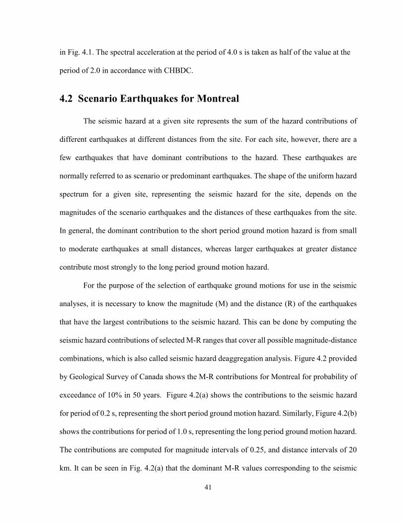
41

in Fig. 4.1. The spectral acceleration at the period of 4.0 s is taken as half of the value at the

period of 2.0 in accordance with CHBDC.

4.2 Scenario Earthquakes for Montreal

The seismic hazard at a given site represents the sum of the hazard contributions of

different earthquakes at different distances from the site. For each site, however, there are a

few earthquakes that have dominant contributions to the hazard. These earthquakes are

normally referred to as scenario or predominant earthquakes. The shape of the uniform hazard

spectrum for a given site, representing the seismic hazard for the site, depends on the

magnitudes of the scenario earthquakes and the distances of these earthquakes from the site.

In general, the dominant contribution to the short period ground motion hazard is from small

to moderate earthquakes at small distances, whereas larger earthquakes at greater distance

contribute most strongly to the long period ground motion hazard.

For the purpose of the selection of earthquake ground motions for use in the seismic

analyses, it is necessary to know the magnitude (M) and the distance (R) of the earthquakes

that have the largest contributions to the seismic hazard. This can be done by computing the

seismic hazard contributions of selected M-R ranges that cover all possible magnitude-distance

combinations, which is also called seismic hazard deaggregation analysis. Figure 4.2 provided

by Geological Survey of Canada shows the M-R contributions for Montreal for probability of

exceedance of 10% in 50 years. Figure 4.2(a) shows the contributions to the seismic hazard

for period of 0.2 s, representing the short period ground motion hazard. Similarly, Figure 4.2(b)

shows the contributions for period of 1.0 s, representing the long period ground motion hazard.

The contributions are computed for magnitude intervals of 0.25, and distance intervals of 20

km. It can be seen in Fig. 4.2(a) that the dominant M-R values corresponding to the seismic

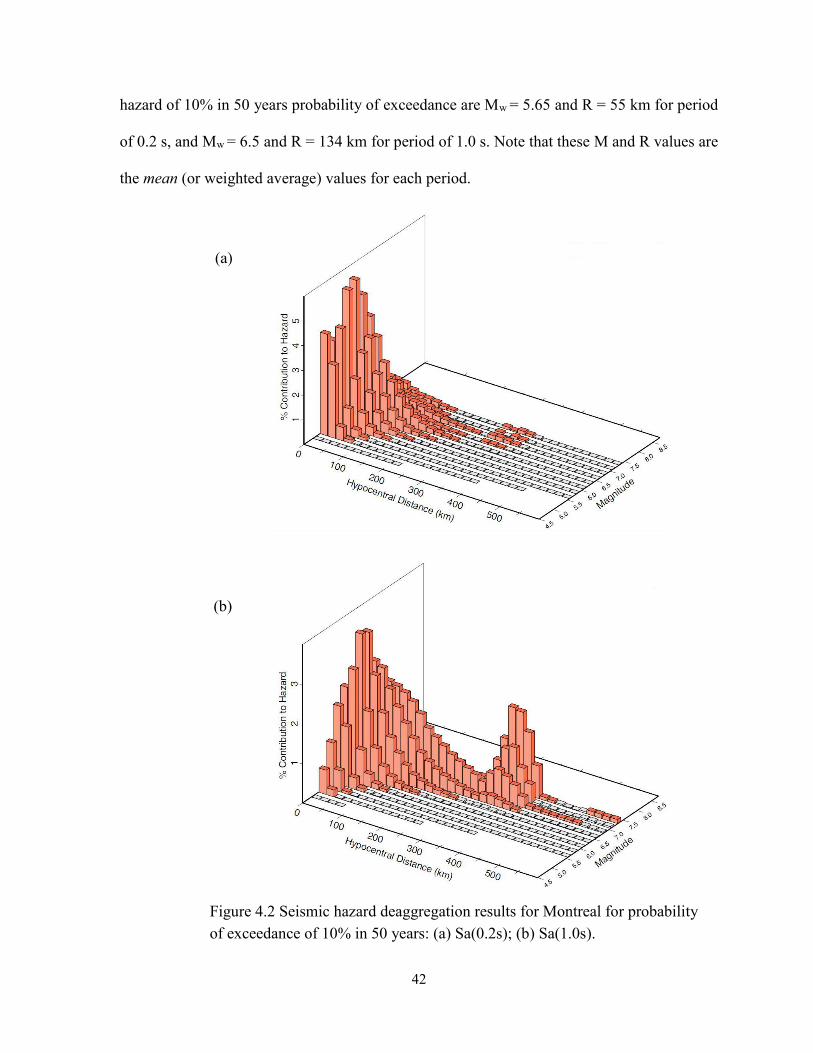
42

hazard of 10% in 50 years probability of exceedance are Mw = 5.65 and R = 55 km for period

of 0.2 s, and Mw = 6.5 and R = 134 km for period of 1.0 s. Note that these M and R values are

the mean (or weighted average) values for each period.

Figure 4.2 Seismic hazard deaggregation results for Montreal for probability

of exceedance of 10% in 50 years: (a) Sa(0.2s); (b) Sa(1.0s).

(a)

(b)

43

4.3 Selection of Records

Ground motion records from earthquakes in Montreal would be the most appropriate

for the time-history analysis of the bridges considered in this study. Since such records are not

available, the records complied by Naumoski et al. (1988 and 1993) were selected.

Due to lack of strong ground motion records in eastern Canada, Naumoski et al. (1988

and 1993) compiled a number of records obtained from earthquakes around the world which

are representative of the characteristics of ground motions in eastern Canada. The records are

grouped into three ensembles, i.e., high A/V set, intermediate A/V set, and low A/V set,

according to the ratio of the peak ground acceleration (in g) to peak ground velocity (in m/s).

The average A/V ratios of the high A/V, intermediate A/V, and low A/V sets are about 2.0,

1.0, and 0.5, respectively. According to Naumoski et al. (1988), seismic motions from small to

moderate earthquakes at short distances are represented by high A/V ratios while those from

large earthquakes at large distances are characterized by low A/V ratios. In terms of the

frequency content, high A/V motions normally have a high frequency content, and low A/V

motions have a low frequency content. Seismic motions with a high frequency content are

characterized by predominant frequencies higher than approximately 2 Hz (i.e., periods lower

than 0.5s), and seismic motions with a low frequency content are characterized by predominant

frequencies lower than 2 Hz (i.e., periods longer 0.5 s).

As reported by Adams and Halchuk (2003); Naumoski et al. (1988), ground motions in

eastern Canada are typically characterized by high frequency content and high A/V ratios.

Given this, the ensemble of the records with high A/V ratios in Naumoski et al. (1988) was

adopted for the analysis. In total, the ensemble consisted of 13 pairs of the horizontal and

vertical components. It is necessary to mention that only horizontal components were used in

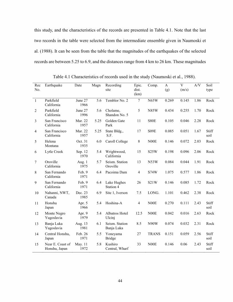
44

this study, and the characteristics of the records are presented in Table 4.1. Note that the last

two records in the table were selected from the intermediate ensemble given in Naumoski et

al. (1988). It can be seen from the table that the magnitudes of the earthquakes of the selected

records are between 5.25 to 6.9, and the distances range from 4 km to 26 km. These magnitudes

Table 4.1 Characteristics of records used in the study (Naumoski et al., 1988).

Rec

No.

Earthquake Date Magn Recording

site

Epic.

dist.

(km)

Comp. A

(g)

V

(m/s)

A/V Soil

type

1 Parkfield

California

June 27

1966

5.6 Temblor No. 2 7 N65W 0.269 0.145 1.86 Rock

2 Parkfield

California

June 27

1996

5.6 Cholame,

Shandon No. 5

5 N85W 0.434 0.255 1.70 Rock

3 San Francisco

California

Mar. 22

1957

5.25 Golden Gate

Park

11 S80E 0.105 0.046 2.28 Rock

4 San Francisco

California

Mar. 22

1957

5.25 State Bldg.,

S.F.

17 S09E 0.085 0.051 1.67 Stiff

soil

5 Helena

Montana

Oct. 31

1935

6.0 Caroll College 8 N00E 0.146 0.072 2.03 Rock

6 Lytle Creek Sep. 12

1970

5.4 Wrightwood,

California

15 S25W 0.198 0.096 2.06 Rock

7 Oroville

California

Aug. 1

1975

5.7 Seism. Station

Oroville

13 N53W 0.084 0.044 1.91 Rock

8 San Fernando

California

Feb. 9

1971

6.4 Pacoima Dam 4 S74W 1.075 0.577 1.86 Rock

9 San Fernando

California

Feb. 9

1971

6.4 Lake Hughes

Station 4

26 S21W 0.146 0.085 1.72 Rock

10 Nahanni, NWT,

Canada

Dec. 23

1985

6.9 Site 1, Iverson 7.5 LONG. 1.101 0.462 2.38 Rock

11 Honshu

Japan

Apr. 5

1966

5.4 Hoshina-A 4 N00E 0.270 0.111 2.43 Stiff

soil

12 Monte Negro

Yugoslavia

Apr. 9

1979

5.4 Albatros Hotel

Ulcinj

12.5 N00E 0.042 0.016 2.63 Rock

13 Banja Luka

Yugoslavia

Aug. 13

1981

6.1 Seism. Station

Banja Luka

8.5 N90W 0.074 0.032 2.31 Rock

14 Central Honshu,

Japan

Feb. 26

1971

5.5 Yoneyama

Bridge

27 TRANS 0.151 0.059 2.56 Stiff

soil

15 Near E. Coast of

Honshu, Japan

May. 11

1972

5.8 Kushiro

Central, Wharf

33 N00E 0.146 0.06 2.43 Stiff

soil

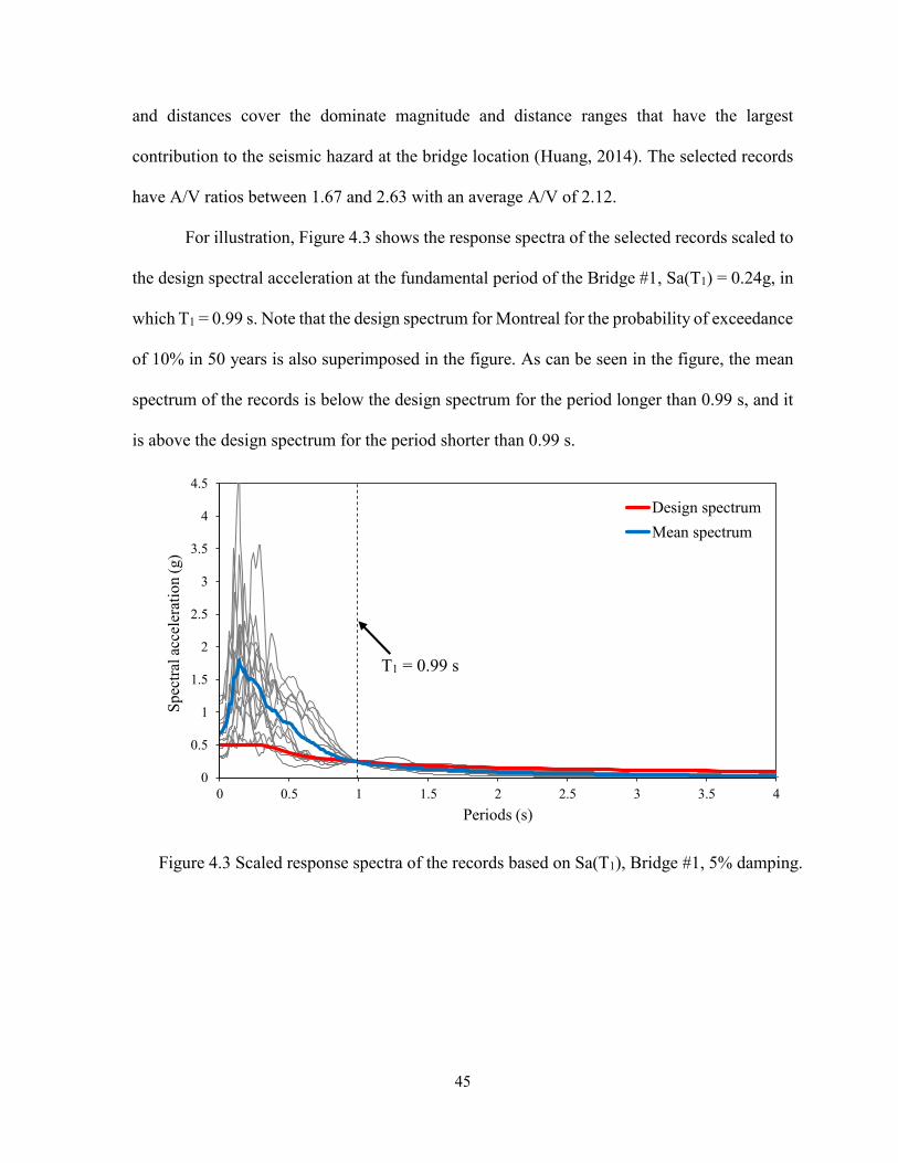
45

and distances cover the dominate magnitude and distance ranges that have the largest

contribution to the seismic hazard at the bridge location (Huang, 2014). The selected records

have A/V ratios between 1.67 and 2.63 with an average A/V of 2.12.

For illustration, Figure 4.3 shows the response spectra of the selected records scaled to

the design spectral acceleration at the fundamental period of the Bridge #1, Sa(T1) = 0.24g, in

which T1 = 0.99 s. Note that the design spectrum for Montreal for the probability of exceedance

of 10% in 50 years is also superimposed in the figure. As can be seen in the figure, the mean

spectrum of the records is below the design spectrum for the period longer than 0.99 s, and it

is above the design spectrum for the period shorter than 0.99 s.

Figure 4.3 Scaled response spectra of the records based on Sa(T1), Bridge #1, 5% damping.

0

0.5

1

1.5

2

2.5

3

3.5

4

4.5

0 0.5 1 1.5 2 2.5 3 3.5 4

Sp

ectr

al a

ccel

erat

ion (

g)

Periods (s)

Design spectrum

Mean spectrum

T1 = 0.99 s

46

Chapter 5

Analysis Results

5.1 Overview

In this study, nonlinear time-history analyses were conducted by subjecting the two

bridge models to the selected records. In order to determine the structural response due to

ground motions with different intensities, the records were scaled to a range of intensity levels

according to Sa(T1). In total, eleven excitation levels were used for the analysis ranged from

0.05 g to 1.20 g for Bridge #1, from 0.05 g to 1.30 g for Bridge #2. Expressed in terms of the

reference spectral acceleration Saref which was determined based on the design spectrum for

Montreal according to CHBDC (2006), the seismic excitations are from 0.2Saref to 5.0Saref.

These intensity levels were selected to cover a wide range of the structural response from

elastic to inelastic in order to assess the effects of the structural modeling parameters on the

seismic response of bridges. The fundamental periods T1 of Bridges #1 and #2 were 0.99 s and

0.89 s, respectively, as described in Chapter 3.

According to the current seismic provisions of the bridge design codes CHBDC (2006)

and AASHTO (2014), all the inelastic deformations during earthquake events should occur in

the substructure while the superstructure should remain elastic. Given this, response

parameters used for the purpose of the study included those representing the behavior of the

superstructure and substructure, respectively. More specifically, a number of response

parameters selected for the study were:

47

deck displacement,

bearing displacement,

column displacement,

column curvature ductility, and

moment at the base of the column.

The deck displacement is a "global" deformation parameter and has been used in a

number of studies for the evaluation of the seismic performance of bridges (e.g., Hwang et al.,

2001; Tavares et al., 2012, etc.). In addition, the gap size between the deck and the abutment

can also be used to represent the displacement of the superstructure (e.g., Pan et al., 2010).

Since the abutments of the two bridges considered in the study were modeled as rollers, gap

size was not used for the investigation.

As reported by Choi et al. (2004), Nielson & DesRoches (2007), and Tavares et al.

(2012), the seismic performance of a bridge depends very much on the behavior of the bearing

which works as a connection between the superstructure and substructure. From the structural

point of view, the displacement of the deck (i.e., displacement of the superstructure) is equal

to the sum of the displacements of the bearing and the column (i.e., displacement of the

substructure). Clearly, the bearing displacement is a "local" response parameter, and it was

used in this study to examine the shear response of the bearing due to the seismic loads. It is

necessary to mention herein that both fixed and expansion bearings were used in the two

bridges, and the fixed bearing only allows the rotation (i.e., translation is not allowed) while

the expansion bearing allows both rotation and translation. The different behavior of the two

types of bearings is discussed in detail in the sections below.

48

The column top displacement is another response parameter used in this investigation.

In knowing the displacement, one can determine the column drift ratio. Unlike the seismic

design of buildings in which the interstorey drift ratio should be limited to 2.5% according to

the National Building Code of Canada (NRCC, 2010), the current edition of CHBDC (2006)

does not specify any limitation on the drift ratio of bridges. It is believed that the results of the

column displacement from this study would be helpful in understanding this issue. In this

study, the displacement of the columns of the two piers in each of bridges were considered.

This is because bearings used on the top of the two piers were different, i.e., fixed bearings

were used on pier 1, while expansion bearings were used on pier 2 (see description in Chapter

3).

The curvature ductility of the column is also a "local" deformation parameter and

represents the extent of inelastic deformations at a specified section of a structural member.

The curvature ductility for a given section of a member represents the ratio of the maximum

curvature (u) experienced during the response to the yield curvature (y) of the section. This

response parameter has been used extensively on the seismic evaluation of bridges, because it

is an indicator of the nonlinearity of the column during earthquake events (e.g., Nielson &

DesRoches, 2006; Pan et al., 2010; Avşar et al., 2011; and Tavares et al., 2012).

The bending moment on the bottom of the column represents one of the "global" force

demands used to design the bridge substructure subjected to seismic loads. A larger moment

indicates that larger seismic force is applied to the column. Please note that shear force was

not considered in the investigation because the nonlinear behavior of the column was defined

using the moment-curvature relation as discussed in Chapter 3.

49

Overall, the response parameters selected in the study covered the responses of both

the superstructure and substructure. They represent both the deformation and force of a given

member during seismic excitations at different levels.

For each excitation motion considered in the study, maximum value of each of the

response parameters mentioned above was computed. Given a large number of analyses

conducted in this study, it is not practical to consider the maximum response from a single

time-history analysis. Therefore, the responses resulting from the set of excitations were

statistically analysed to compute the mean (M) value. The use of the mean values is considered

appropriate because these values are more "stable" (i.e., they have smaller variations) than the

mean plus one standard deviation (M+SD) values.

As given in Chapter 1 (Introduction), the main objective of the study was to investigate

the effects of the different modeling parameters on the seismic response of bridges. More

specifically, the following modeling parameters were considered in the analysis,

Superstructure mass,

Concrete compressive strength,

Yield strength of the reinforcing steel,

Yield displacement of the bearing,

Post-yield stiffness of the bearing,

Plastic hinge length, and

Damping.

Nonlinear time-history analyses were conducted by changing the nominal value of each

modeling parameter by a range of factors. The nominal value of each parameter along with its

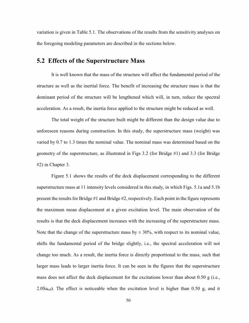
50

variation is given in Table 5.1. The observations of the results from the sensitivity analyses on

the foregoing modeling parameters are described in the sections below.

5.2 Effects of the Superstructure Mass

It is well known that the mass of the structure will affect the fundamental period of the

structure as well as the inertial force. The benefit of increasing the structure mass is that the

dominant period of the structure will be lengthened which will, in turn, reduce the spectral

acceleration. As a result, the inertia force applied to the structure might be reduced as well.

The total weight of the structure built might be different than the design value due to

unforeseen reasons during construction. In this study, the superstructure mass (weight) was

varied by 0.7 to 1.3 times the nominal value. The nominal mass was determined based on the

geometry of the superstructure, as illustrated in Figs 3.2 (for Bridge #1) and 3.3 (for Bridge

#2) in Chapter 3.

Figure 5.1 shows the results of the deck displacement corresponding to the different

superstructure mass at 11 intensity levels considered in this study, in which Figs. 5.1a and 5.1b

present the results for Bridge #1 and Bridge #2, respectively. Each point in the figure represents

the maximum mean displacement at a given excitation level. The main observation of the

results is that the deck displacement increases with the increasing of the superstructure mass.

Note that the change of the superstructure mass by ± 30%, with respect to its nominal value,

shifts the fundamental period of the bridge slightly, i.e., the spectral acceleration will not

change too much. As a result, the inertia force is directly proportional to the mass, such that

larger mass leads to larger inertia force. It can be seen in the figures that the superstructure

mass does not affect the deck displacement for the excitations lower than about 0.50 g (i.e.,

2.0Saref). The effect is noticeable when the excitation level is higher than 0.50 g, and it

51

increases with the intensity level. Table 5.2 presents the maximum differences of the deck

displacements resulting from the variation of the superstructure mass with respect to the

reference response at typical intensity levels. The reference response refers to the response

based on the nominal mass, which is designated as "100% Super mass" in the figures in this

section (Figs. 5.1 to 5.8). The results in Table 5.2 show that the change of the superstructure

mass by 30% causes the change of the displacement by 9.4% of the reference response at the

highest intensity level, 5.0Saref. It indicates that the superstructure mass does not have

significant effect on the deck displacement.

The findings of the results for the maximum moment on the base of the column (Fig.

5.2) are similar to those of the deck displacement, i.e., larger mass leads to larger moment.

Like for the deck displacement, the effects of the superstructure mass on the bending moment

are noticeable starting at the intensity level about 0.50 g (i.e., 2.0Saref). By comparing the

resulted differences for the moment with those for the deck displacement shown in Table 5.2,

it can be concluded that the effect of the change of the superstructure mass on the bending

moment on the base of column is relatively larger compared to that on the deck displacement.

The results for the bearing displacements of Bridge #1 and Bridge #2 are illustrated in

Figs. 5.3 and 5.4 respectively, in which Fig. 5.3 presents the results for the fixed bearing and

Fig. 5.4 for the expansion bearing. The results in the figures show that the bearing displacement

increases with the increasing of the superstructure mass, except for the fixed bearing on Bridge

#1 (Fig. 5.3a) where the displacement from the 85% of the nominal superstructure mass is

significantly larger than the reference value. This might be due to the redistribution of the

seismic force during nonlinear behavior of the bridge. Another observation of the results in

Fig. 5.3 is that the superstructure mass has noticeable effect starting at 0.24 g for Bridge #1,

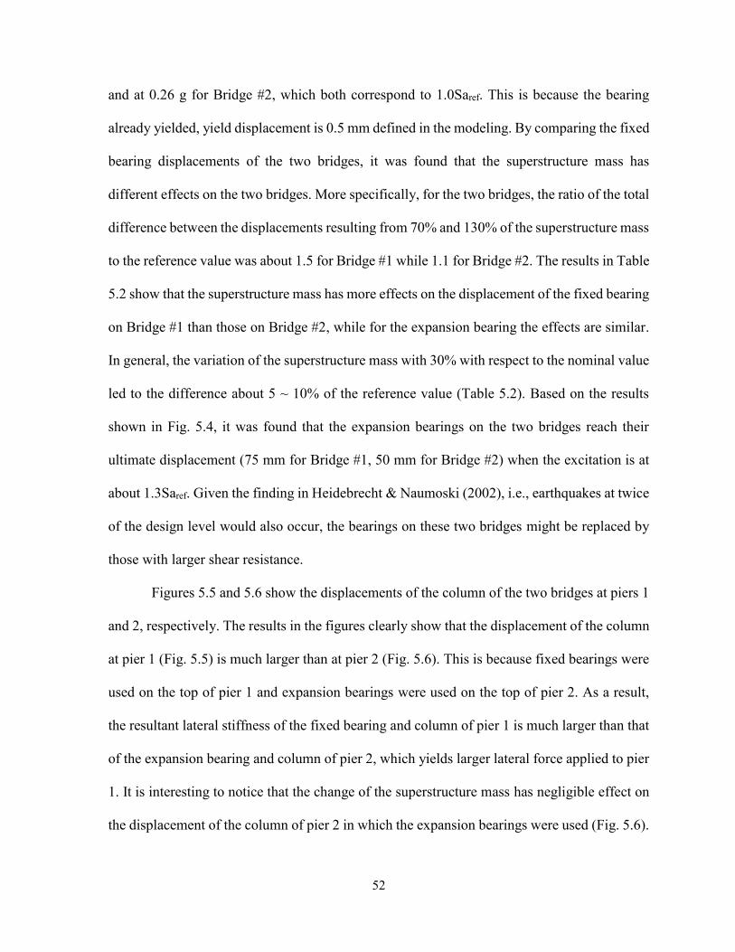
52

and at 0.26 g for Bridge #2, which both correspond to 1.0Saref. This is because the bearing

already yielded, yield displacement is 0.5 mm defined in the modeling. By comparing the fixed

bearing displacements of the two bridges, it was found that the superstructure mass has

different effects on the two bridges. More specifically, for the two bridges, the ratio of the total

difference between the displacements resulting from 70% and 130% of the superstructure mass

to the reference value was about 1.5 for Bridge #1 while 1.1 for Bridge #2. The results in Table

5.2 show that the superstructure mass has more effects on the displacement of the fixed bearing

on Bridge #1 than those on Bridge #2, while for the expansion bearing the effects are similar.

In general, the variation of the superstructure mass with 30% with respect to the nominal value

led to the difference about 5 ~ 10% of the reference value (Table 5.2). Based on the results

shown in Fig. 5.4, it was found that the expansion bearings on the two bridges reach their

ultimate displacement (75 mm for Bridge #1, 50 mm for Bridge #2) when the excitation is at

about 1.3Saref. Given the finding in Heidebrecht & Naumoski (2002), i.e., earthquakes at twice

of the design level would also occur, the bearings on these two bridges might be replaced by

those with larger shear resistance.

Figures 5.5 and 5.6 show the displacements of the column of the two bridges at piers 1

and 2, respectively. The results in the figures clearly show that the displacement of the column

at pier 1 (Fig. 5.5) is much larger than at pier 2 (Fig. 5.6). This is because fixed bearings were

used on the top of pier 1 and expansion bearings were used on the top of pier 2. As a result,

the resultant lateral stiffness of the fixed bearing and column of pier 1 is much larger than that

of the expansion bearing and column of pier 2, which yields larger lateral force applied to pier

1. It is interesting to notice that the change of the superstructure mass has negligible effect on

the displacement of the column of pier 2 in which the expansion bearings were used (Fig. 5.6).

53

Based on the results shown in Table 5.2, it was found that on average the change of the

superstructure mass by 30% will change the displacement of the column of pier 1 by about 8%,

where fixed bearings were installed.

The results for the column curvature ductility are presented in Figs. 5.7 and 5.8, in

which Fig. 5.7 is for the column at pier 1 (fixed bearings were used) and Fig. 5.8 is for the

column at pier 2 (expansion bearings were used). By comparing the results shown in the

figures, it can be seen that the change of the superstructure mass has less effect on the column

at pier 2 (Fig. 5.8 and Table 5.2). This is because pier 1 takes a greater amount of the total

seismic load than pier 2, due to the larger resultant lateral stiffness of pier 1 as discussed above.

The results in the figures also show that all the fixed bearings on the two bridges yield at the

excitation level of about 0.25 g which corresponds to 1.0Saref (i.e., the design earthquake level)

because the ductility is greater than 1.0. Therefore, it is wise to increase the size of the bearings

such that they can sustain during larger earthquakes that might occur in the future. As given in

Table 5.2, for Bridge #1, the 30% changing of the superstructure mass creates on average about

5% difference of the pier ductility.

5.3 Effects of the Concrete Compressive Strength

The uncertainty of the material property is one of the factors that is taken into account

in the assessment of the seismic fragility of bridges as given in Choi et al. (2004), Pan et al.

(2010), and Tavares et al. (2012). In terms of the nonlinear time-history analysis, it is known

that the concrete compressive strength (fc') would affect the result of the moment-curvature or

moment-rotation relationship of a given reinforced concrete section in addition to its capacity.

For illustration, Figure 5.9 shows the moment-curvature relationships of an end section on the

bottom of the column at pier 1 on Bridge #1 using fc' = 20 MPa and fc

' = 40 MPa, respectively.

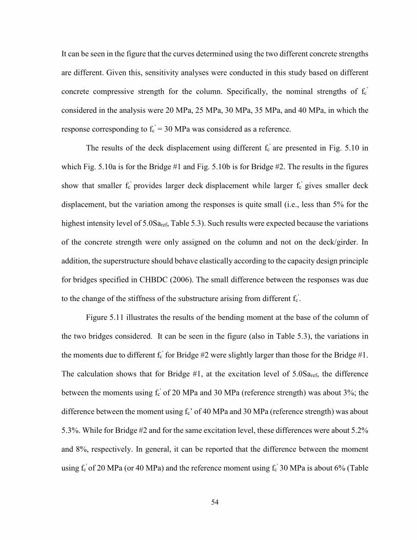
54

It can be seen in the figure that the curves determined using the two different concrete strengths

are different. Given this, sensitivity analyses were conducted in this study based on different

concrete compressive strength for the column. Specifically, the nominal strengths of fc’

considered in the analysis were 20 MPa, 25 MPa, 30 MPa, 35 MPa, and 40 MPa, in which the

response corresponding to fc' = 30 MPa was considered as a reference.

The results of the deck displacement using different fc' are presented in Fig. 5.10 in

which Fig. 5.10a is for the Bridge #1 and Fig. 5.10b is for Bridge #2. The results in the figures

show that smaller fc' provides larger deck displacement while larger fc

' gives smaller deck

displacement, but the variation among the responses is quite small (i.e., less than 5% for the

highest intensity level of 5.0Saref, Table 5.3). Such results were expected because the variations

of the concrete strength were only assigned on the column and not on the deck/girder. In

addition, the superstructure should behave elastically according to the capacity design principle

for bridges specified in CHBDC (2006). The small difference between the responses was due

to the change of the stiffness of the substructure arising from different fc'.

Figure 5.11 illustrates the results of the bending moment at the base of the column of

the two bridges considered. It can be seen in the figure (also in Table 5.3), the variations in

the moments due to different fc' for Bridge #2 were slightly larger than those for the Bridge #1.

The calculation shows that for Bridge #1, at the excitation level of 5.0Saref, the difference

between the moments using fc' of 20 MPa and 30 MPa (reference strength) was about 3%; the

difference between the moment using fc’ of 40 MPa and 30 MPa (reference strength) was about

5.3%. While for Bridge #2 and for the same excitation level, these differences were about 5.2%

and 8%, respectively. In general, it can be reported that the difference between the moment

using fc' of 20 MPa (or 40 MPa) and the reference moment using fc

' 30 MPa is about 6% (Table

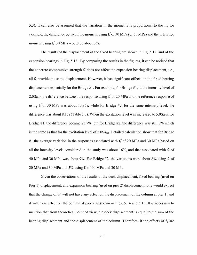
55

5.3). It can also be assumed that the variation in the moments is proportional to the fc', for

example, the difference between the moment using fc' of 30 MPa (or 35 MPa) and the reference

moment using fc' 30 MPa would be about 3%.

The results of the displacement of the fixed bearing are shown in Fig. 5.12, and of the

expansion bearings in Fig. 5.13. By comparing the results in the figures, it can be noticed that

the concrete compressive strength fc' does not affect the expansion bearing displacement, i.e.,

all fc' provide the same displacement. However, it has significant effects on the fixed bearing

displacement especially for the Bridge #1. For example, for Bridge #1, at the intensity level of

2.0Saref, the difference between the response using fc' of 20 MPa and the reference response of

using fc' of 30 MPa was about 13.8%; while for Bridge #2, for the same intensity level, the

difference was about 8.1% (Table 5.3). When the excitation level was increased to 5.0Saref, for

Bridge #1, the difference became 23.7%, but for Bridge #2, the difference was still 8% which

is the same as that for the excitation level of 2.0Saref. Detailed calculation show that for Bridge

#1 the average variation in the responses associated with fc' of 20 MPa and 30 MPa based on

all the intensity levels considered in the study was about 16%, and that associated with fc' of

40 MPa and 30 MPa was about 9%. For Bridge #2, the variations were about 8% using fc' of

20 MPa and 30 MPa and 5% using fc' of 40 MPa and 30 MPa.

Given the observations of the results of the deck displacement, fixed bearing (used on

Pier 1) displacement, and expansion bearing (used on pier 2) displacement, one would expect

that the change of fc’ will not have any effect on the displacement of the column at pier 1, and

it will have effect on the column at pier 2 as shown in Figs. 5.14 and 5.15. It is necessary to

mention that from theoretical point of view, the deck displacement is equal to the sum of the

bearing displacement and the displacement of the column. Therefore, if the effects of fc' are

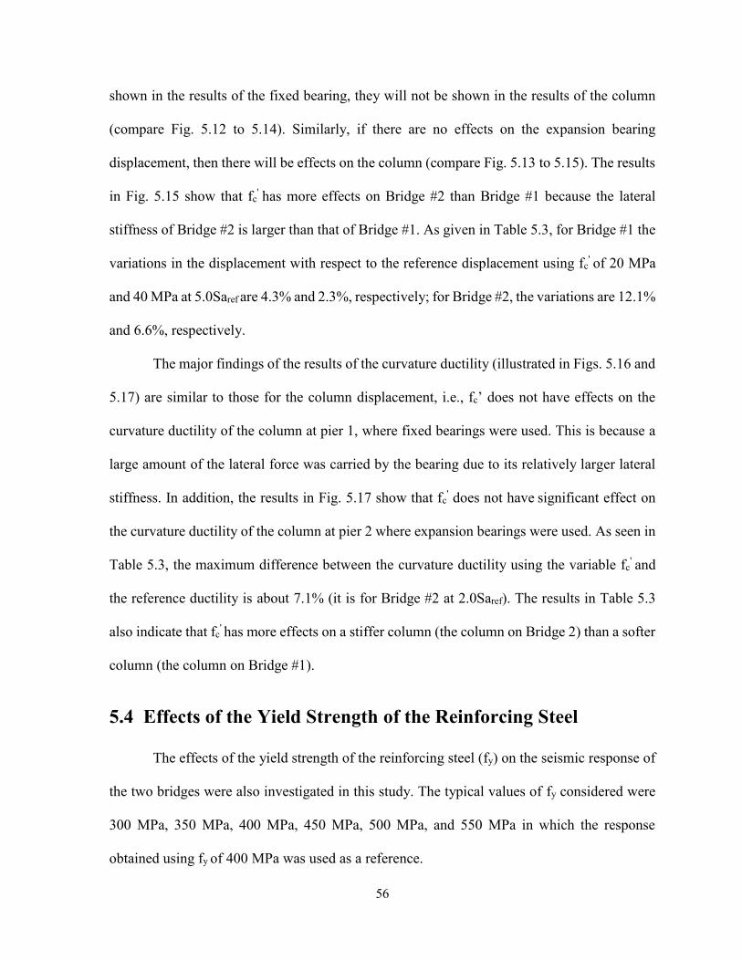
56

shown in the results of the fixed bearing, they will not be shown in the results of the column

(compare Fig. 5.12 to 5.14). Similarly, if there are no effects on the expansion bearing

displacement, then there will be effects on the column (compare Fig. 5.13 to 5.15). The results

in Fig. 5.15 show that fc' has more effects on Bridge #2 than Bridge #1 because the lateral

stiffness of Bridge #2 is larger than that of Bridge #1. As given in Table 5.3, for Bridge #1 the

variations in the displacement with respect to the reference displacement using fc' of 20 MPa

and 40 MPa at 5.0Saref are 4.3% and 2.3%, respectively; for Bridge #2, the variations are 12.1%

and 6.6%, respectively.

The major findings of the results of the curvature ductility (illustrated in Figs. 5.16 and

5.17) are similar to those for the column displacement, i.e., fc’ does not have effects on the

curvature ductility of the column at pier 1, where fixed bearings were used. This is because a

large amount of the lateral force was carried by the bearing due to its relatively larger lateral

stiffness. In addition, the results in Fig. 5.17 show that fc' does not have significant effect on

the curvature ductility of the column at pier 2 where expansion bearings were used. As seen in

Table 5.3, the maximum difference between the curvature ductility using the variable fc' and

the reference ductility is about 7.1% (it is for Bridge #2 at 2.0Saref). The results in Table 5.3

also indicate that fc' has more effects on a stiffer column (the column on Bridge 2) than a softer

column (the column on Bridge #1).

5.4 Effects of the Yield Strength of the Reinforcing Steel

The effects of the yield strength of the reinforcing steel (fy) on the seismic response of

the two bridges were also investigated in this study. The typical values of fy considered were

300 MPa, 350 MPa, 400 MPa, 450 MPa, 500 MPa, and 550 MPa in which the response

obtained using fy of 400 MPa was used as a reference.

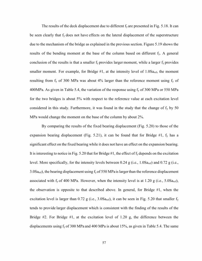
57

The results of the deck displacement due to different fy are presented in Fig. 5.18. It can

be seen clearly that fy does not have effects on the lateral displacement of the superstructure

due to the mechanism of the bridge as explained in the previous section. Figure 5.19 shows the

results of the bending moment at the base of the column based on different fy. A general

conclusion of the results is that a smaller fy provides larger moment, while a larger fy provides

smaller moment. For example, for Bridge #1, at the intensity level of 1.0Saref, the moment

resulting from fy of 300 MPa was about 4% larger than the reference moment using fy of

400MPa. As given in Table 5.4, the variation of the response using fy of 300 MPa or 550 MPa

for the two bridges is about 5% with respect to the reference value at each excitation level

considered in this study. Furthermore, it was found in the study that the change of fy by 50

MPa would change the moment on the base of the column by about 2%.

By comparing the results of the fixed bearing displacement (Fig. 5.20) to those of the

expansion bearing displacement (Fig. 5.21), it can be found that for Bridge #1, fy has a

significant effect on the fixed bearing while it does not have an effect on the expansion bearing.

It is interesting to notice in Fig. 5.20 that for Bridge #1, the effect of fy depends on the excitation

level. More specifically, for the intensity levels between 0.24 g (i.e., 1.0Saref) and 0.72 g (i.e.,

3.0Saref), the bearing displacement using fy of 550 MPa is larger than the reference displacement

associated with fy of 400 MPa. However, when the intensity level is at 1.20 g (i.e., 5.0Saref),

the observation is opposite to that described above. In general, for Bridge #1, when the

excitation level is larger than 0.72 g (i.e., 3.0Saref), it can be seen in Fig. 5.20 that smaller fy

tends to provide larger displacement which is consistent with the finding of the results of the

Bridge #2. For Bridge #1, at the excitation level of 1.20 g, the difference between the

displacements using fy of 300 MPa and 400 MPa is about 15%, as given in Table 5.4. The same

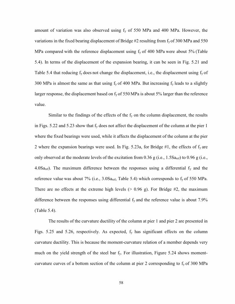
58

amount of variation was also observed using fy of 550 MPa and 400 MPa. However, the

variations in the fixed bearing displacement of Bridge #2 resulting from fy of 300 MPa and 550

MPa compared with the reference displacement using fy of 400 MPa were about 5% (Table

5.4). In terms of the displacement of the expansion bearing, it can be seen in Fig. 5.21 and

Table 5.4 that reducing fy does not change the displacement, i.e., the displacement using fy of

300 MPa is almost the same as that using fy of 400 MPa. But increasing fy leads to a slightly

larger response, the displacement based on fy of 550 MPa is about 5% larger than the reference

value.

Similar to the findings of the effects of the fy on the column displacement, the results

in Figs. 5.22 and 5.23 show that fy does not affect the displacement of the column at the pier 1

where the fixed bearings were used, while it affects the displacement of the column at the pier

2 where the expansion bearings were used. In Fig. 5.23a, for Bridge #1, the effects of fy are

only observed at the moderate levels of the excitation from 0.36 g (i.e., 1.5Saref) to 0.96 g (i.e.,

4.0Saref). The maximum difference between the responses using a differential fy and the

reference value was about 7% (i.e., 3.0Saref, Table 5.4) which corresponds to fy of 550 MPa.

There are no effects at the extreme high levels (> 0.96 g). For Bridge #2, the maximum

difference between the responses using differential fy and the reference value is about 7.9%

(Table 5.4).

The results of the curvature ductility of the column at pier 1 and pier 2 are presented in

Figs. 5.25 and 5.26, respectively. As expected, fy has significant effects on the column

curvature ductility. This is because the moment-curvature relation of a member depends very

much on the yield strength of the steel bar fy. For illustration, Figure 5.24 shows moment-

curvature curves of a bottom section of the column at pier 2 corresponding to fy of 300 MPa

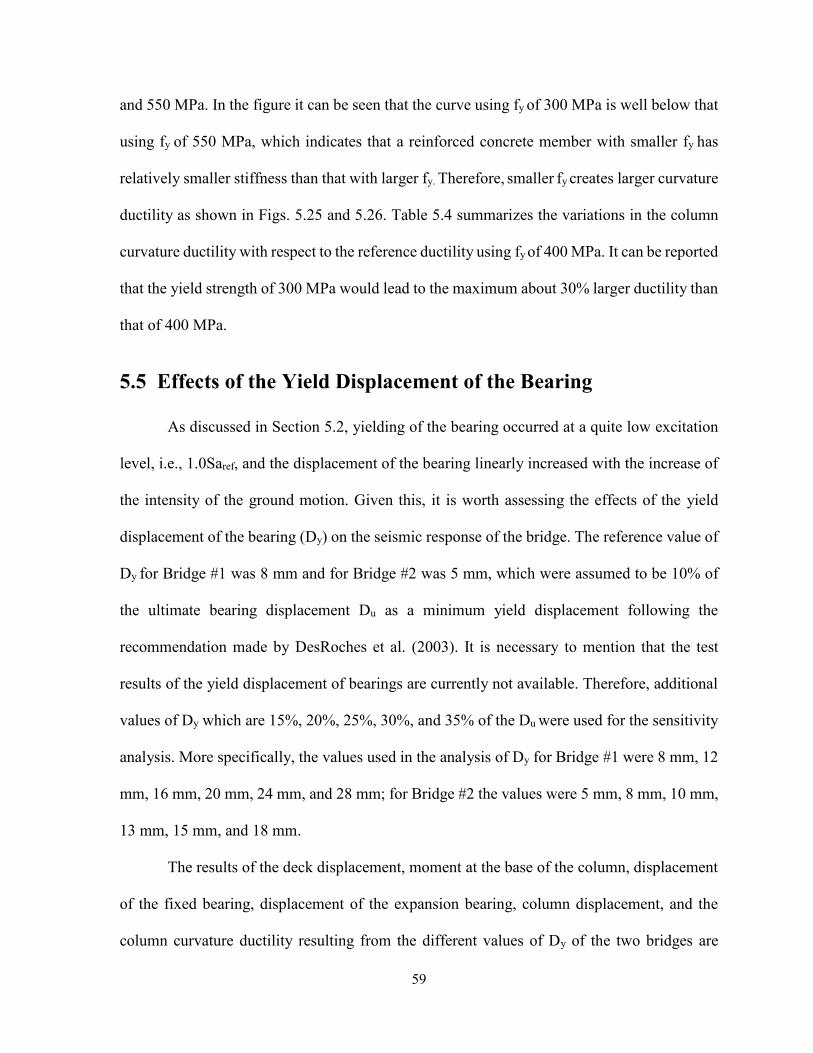
59

and 550 MPa. In the figure it can be seen that the curve using fy of 300 MPa is well below that

using fy of 550 MPa, which indicates that a reinforced concrete member with smaller fy has

relatively smaller stiffness than that with larger fy. Therefore, smaller fy creates larger curvature

ductility as shown in Figs. 5.25 and 5.26. Table 5.4 summarizes the variations in the column

curvature ductility with respect to the reference ductility using fy of 400 MPa. It can be reported

that the yield strength of 300 MPa would lead to the maximum about 30% larger ductility than

that of 400 MPa.

5.5 Effects of the Yield Displacement of the Bearing

As discussed in Section 5.2, yielding of the bearing occurred at a quite low excitation

level, i.e., 1.0Saref, and the displacement of the bearing linearly increased with the increase of

the intensity of the ground motion. Given this, it is worth assessing the effects of the yield

displacement of the bearing (Dy) on the seismic response of the bridge. The reference value of

Dy for Bridge #1 was 8 mm and for Bridge #2 was 5 mm, which were assumed to be 10% of

the ultimate bearing displacement Du as a minimum yield displacement following the

recommendation made by DesRoches et al. (2003). It is necessary to mention that the test

results of the yield displacement of bearings are currently not available. Therefore, additional

values of Dy which are 15%, 20%, 25%, 30%, and 35% of the Du were used for the sensitivity

analysis. More specifically, the values used in the analysis of Dy for Bridge #1 were 8 mm, 12

mm, 16 mm, 20 mm, 24 mm, and 28 mm; for Bridge #2 the values were 5 mm, 8 mm, 10 mm,

13 mm, 15 mm, and 18 mm.

The results of the deck displacement, moment at the base of the column, displacement

of the fixed bearing, displacement of the expansion bearing, column displacement, and the

column curvature ductility resulting from the different values of Dy of the two bridges are

60

presented in Figs. 5.27 to 5.34. It can be seen in the figures that the change of Dy does not

affect the response parameters mentioned above except the displacement and the curvature

ductility of the column at pier 2 where the expansion bearings were used. This is because the

initial elastic stiffness of the bearing does not depend on Dy, it depends on the geometry of the

bearing including the plan area of the bearing pad, and the total thickness of the elastomer. In

other words, the elastic stiffness K1 of the bearing (Fig. 3.6, Chapter 3) was kept constant in the

analysis, in which K1 was 1500 kN/m for Bridge #1, 7000 kN/m for Bridge #2 as provided in

Table 3.1, Chapter 3 These values were determined by using Dy of 8 mm for Bridge #1, 5 mm

for Bridge #2, respectively. If the stiffness of the bearing does not change, the total lateral

stiffness of the bridge will not change as well. In addition, it was assumed that no stiffness

degradation occurred during nonlinear behavior of the bearing, i.e., the degrading stiffness of

the bearing is the same as the initial elastic stiffness (Fig. 3.10, Chapter 3). As a result, the deck

displacement, the fixed bearing displacement and the expansion bearing displacement did not

change with Dy. As illustrated in Fig. 5.32 and 5.34, the change of Dy only affects the

displacement and curvature ductility of the column at pier 2 Bridge #2, where the expansion

bearings were used. This is due to the fact that the column at the pier 2 behaved elastically

(curvature ductility is less than 1.0, Fig. 5.34). Therefore, the response increased linearly with

Dy. For both parameters, the response resulting from Dy of 18 mm was about 40% (38.3% and

43.1% for the column top displacement, and column curvature ductility at pier 2, respectively)

larger than the reference value at the excitation level of 1.0Saref, and was about 10.1% at the

excitation level of 5.0SaRef (Table 5.5).

61

5.6 Effects of the Post-yield Stiffness of the Bearing

As described in Chapter 3, the post-yield stiffness (K2) was considered to be 1/3 times

the initial elastic stiffness (K1) in modeling the nonlinear behavior of the bearing. The factor

1/3 was suggested by on Hwang et al. (2001) and DesRoches et al. (2003). In order to assess

the effects of the post-yield stiffness K2 of the bearing on the response of the bridge, different

values for the K2 were used in the investigation which were 0, 0.3, 0.5, and 0.7. It is necessary

to mention that K2 of 0 represents elastic-perfectly-plastic hysteretic behavior of the bearing

during earthquake events. Among the four values considered, 0.3 was used as a reference.


of the fixed bearing, displacement of the expansion bearing, column displacement, and the

column curvature ductility associated with different values of K2 of the two bridges are

illustrated in Figs. 5.35 to 5.42. It can be seen in the figures that the effects of K2 on the deck

displacement (Fig. 5.35), moment at the base of the column (Fig. 5.36), displacement of the

fixed bearing (Fig. 5.37), displacement of column at pier 1 (Fig. 5.39), and curvature ductility

of the column at pier 1 (Fig. 5.41) are very similar, i.e., for each of the parameters mentioned

above, the responses provided by K2 of 0.3, 0.5, and 0.7 are very close. The response using K2

of 0 is larger than the reference response using K2 of 0.3, in which the maximum difference is

about 7% for the intensity level of 5.0Sa(T1).

In this study, it was found that K2 had significant effects on the displacement of the

expansion bearing (Fig. 5.38), displacement and curvature ductility of the column at pier 2

(Figs. 5.40 and 5.42, respectively) where expansion bearings were installed. In terms of the

expansion bearing displacement, the results showed that K2 of 0 provided the largest response

and K2 of 0.7 provided the smallest response. The calculation shows that for Bridge #1, for the

62

excitation level of 1.0Saref, the bearing displacement corresponding to K2 of 0 is about 17.1%

larger than the reference response using K2 of 0.3; and for the excitation level of 5.0Saref, is

about 37% larger than the reference displacement. These differences became 15.6% and 20.4%

when K2 of 0.7 was used as listed in Table 5.6. As shown in Fig. 5.38 and Table 5.6, the

variations in the displacement due to different values of K2 for Bridge #2 are smaller than those

for Bridge #1. In general, for Bridge #2, the difference between the displacements using K2 of

0 or K2 of 0.7 with respect to the reference value is about 10 ~ 20%.

The observations of the results of the displacement and curvature ductility of the

column at pier 2 (Figs. 5.40 and 5.42, respectively) are very similar, i.e., for Bridge #1, K2 of

0.3, 0.5, and 0.7 created almost the same response, while K2 of 0 provided relatively larger

response, which is about 40% greater than the reference value using K2 of 0.3 at the intensity

level of 5.0Sa(T1) (Table 5.6). However, for Bridge #2, K2 of 0.7 provided the largest response;

K2 of 0 provided the smallest response, while the response using K2 of 0.3 is approximately

in-between those using K2 of 0.7 and K2 of 0. As given in Table 5.6, for all the excitation levels

considered in the study, the response including displacement and curvature ductility of the

column at pier 2 resulting from K2 of 0.7 is 66.9 ~ 89.3% larger than the reference value from

K2 of 0.3, and that resulting from K2 of 0.0 is 39.3~ 51.8% smaller than the reference value

from K2 of 0.3.

5.7 Effects of the Plastic Hinge Length

In order to evaluate the effects of the plastic hinge length on the seismic response of

bridge, in this study the plastic hinge length Lp was varied by a factor of 1.1 to 1.5 times its

nominal value which was 1 m for Bridge #1, 0.72 m for Bridge #2 according to CHBDC

63

(2006). The nominal value of Lp was considered as a reference value for the purpose of

comparing the results.

The results of the response parameters corresponding to different plastic hinge length

showed that the change of the Lp did not affect the deck displacement (Fig. 5.43), displacements

of the fixed bearing and expansion bearing (Figs. 5.45 and 5.46, respectively), and

displacements of the column at pier 1 (Fig. 5.47) and pier 2 (Fig. 5.48), i.e., all the values of

Lp provided the same response. This is because the lateral stiffness of the bridge substructure

only depends on the plan dimensions of the bearing pad and cross-sectional dimensions of the

column, it is not related to the plastic hinge length. On the contrary, the plastic hinge length

has significant effects on the bending moment at the base of the column and the column

curvature ductility as discussed below.

The results of the bending moment at the base of the column resulting from different

values of Lp are presented in Fig. 5.44. It can be clearly seen in the figure that larger Lp provides

relatively small moment. It was found in this study that increasing every 10% of Lp would

reduce the corresponding moment by 3%. For example, for Bridge #1, the bending moment at

the base of the column based on reference Lp of 1.0 m, on average, is about 15% greater than

the moment while that using Lp of 1.5 m (i.e., 50% larger than the reference Lp) as listed in

Table 5.7. Similar observations were obtained from the results of the column curvature

ductility, i.e., larger plastic hinge length led to smaller ductility. Furthermore, it was noticed

that the change of the plastic hinge length by 10% would create around 2% difference in the

response. For example, the Lp of 1.5 m for Bridge #1, 1.08 m for Bridge #2 which was 50%

larger than the nominal value, gave the curvature ductility about 7 ~ 9% less than the reference

ductility, as shown in Table 5.7.

64

5.8 Effects of Damping

In addition to the modeling parameters mentioned above, damping was another

parameter used to assess the seismic response of bridge in this study. In the modeling of the

two bridges, Rayleigh damping was considered in order to take into account the stiffness

degradation of the bridge during nonlinear response, and a nominal value of the damping of

5% was applied to all the 12 vibration modes. For the purpose of the investigation, the

variation of damping ranged from 2% to 8%, in which the 5% damping was considered as a

reference to compare the analysis results.


of the fixed bearing, displacement of the expansion bearing, displacement of the column at pier

1, displacement of the column at pier 2, curvature ductility of the column at pier 1 where the

fixed bearings were used, curvature ductility of the column at pier 2 on which expansion

bearings were used are presented in Figs. 5.51 to 5.58, respectively. As expected, smaller

damping provides larger response while larger damping creates smaller response. Detailed

calculations showed that change of the damping by 1% would create variation on average about

3% in all the response parameters considered. Unlike Bridge #2 in which the variations in the

response were almost the same for all the excitation levels (Table 5.8), for Bridge #1, the

difference between the response using damping less than 5% and the reference response (using

5% damping) was extremely high at the lower excitation level for some of the response

parameters. For example, as seen in Table 5.8, at the intensity level of 1.0Saref, both the column

displacement and the curvature ductility of the column at pier 2 resulting from 2% damping is

about 17% larger than the reference value (Table 5.8). However, at the excitation level of

5.0Saref, it is only 9% larger than the reference ductility. Such results indicate that damping

65

might have significant effects on a certain type of bridge (e.g., Bridge #1 in this study) during

elastic analysis for a relatively low excitation level. Based on the results of the two bridges

listed in Table 5.8, it was found that the response based on damping of 2% on average was

about 10% larger than the reference response, while that based on damping of 8% was around

8% smaller than the reference.

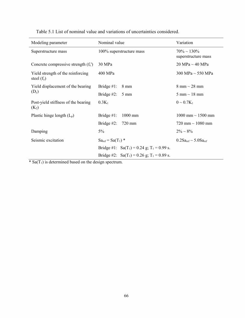
66

Table 5.1 List of nominal value and variations of uncertainties considered.

Modeling parameter Nominal value Variation

Superstructure mass 100% superstructure mass 70% ~ 130%

superstructure mass

Concrete compressive strength (fc') 30 MPa 20 MPa ~ 40 MPa

Yield strength of the reinforcing

steel (fy)

400 MPa 300 MPa ~ 550 MPa

Yield displacement of the bearing

(Dy)

Bridge #1: 8 mm 8 mm ~ 28 mm

Bridge #2: 5 mm 5 mm ~ 18 mm

Post-yield stiffness of the bearing

(K2)

0.3K1 0 ~ 0.7K1

Plastic hinge length (Lp) Bridge #1: 1000 mm 1000 mm ~ 1500 mm

Bridge #2: 720 mm 720 mm ~ 1080 mm

Damping 5% 2% ~ 8%

Seismic excitation Saref = Sa(T1) *

Bridge #1: Sa(T1) = 0.24 g; T1 = 0.99 s.

Bridge #2: Sa(T1) = 0.26 g; T1 = 0.89 s.

0.2Saref ~ 5.0Saref

* Sa(T1) is determined based on the design spectrum.

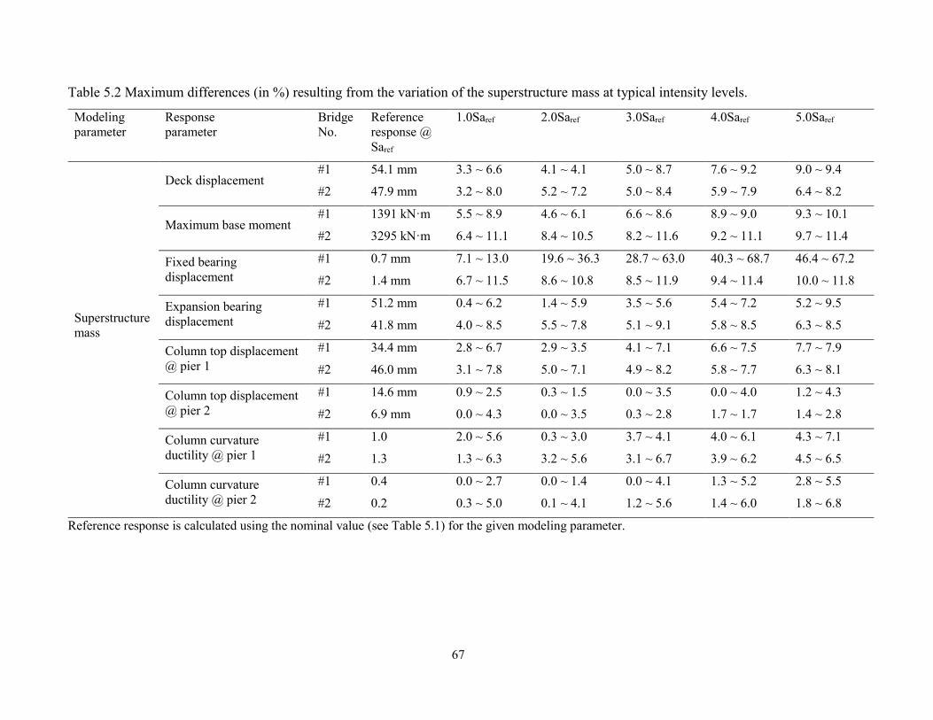
67

Table 5.2 Maximum differences (in %) resulting from the variation of the superstructure mass at typical intensity levels.

Reference response is calculated using the nominal value (see Table 5.1) for the given modeling parameter.

Modeling

parameter

Response

parameter

Bridge

No.

Reference

response @

Saref

1.0Saref 2.0Saref 3.0Saref 4.0Saref 5.0Saref

Superstructure

mass

Deck displacement #1 54.1 mm 3.3 ~ 6.6 4.1 ~ 4.1 5.0 ~ 8.7 7.6 ~ 9.2 9.0 ~ 9.4

#2 47.9 mm 3.2 ~ 8.0 5.2 ~ 7.2 5.0 ~ 8.4 5.9 ~ 7.9 6.4 ~ 8.2

Maximum base moment #1 1391 kN·m 5.5 ~ 8.9 4.6 ~ 6.1 6.6 ~ 8.6 8.9 ~ 9.0 9.3 ~ 10.1

#2 3295 kN·m 6.4 ~ 11.1 8.4 ~ 10.5 8.2 ~ 11.6 9.2 ~ 11.1 9.7 ~ 11.4

Fixed bearing

displacement

#1 0.7 mm 7.1 ~ 13.0 19.6 ~ 36.3 28.7 ~ 63.0 40.3 ~ 68.7 46.4 ~ 67.2

#2 1.4 mm 6.7 ~ 11.5 8.6 ~ 10.8 8.5 ~ 11.9 9.4 ~ 11.4 10.0 ~ 11.8

Expansion bearing

displacement

#1 51.2 mm 0.4 ~ 6.2 1.4 ~ 5.9 3.5 ~ 5.6 5.4 ~ 7.2 5.2 ~ 9.5

#2 41.8 mm 4.0 ~ 8.5 5.5 ~ 7.8 5.1 ~ 9.1 5.8 ~ 8.5 6.3 ~ 8.5

Column top displacement

@ pier 1

#1 34.4 mm 2.8 ~ 6.7 2.9 ~ 3.5 4.1 ~ 7.1 6.6 ~ 7.5 7.7 ~ 7.9

#2 46.0 mm 3.1 ~ 7.8 5.0 ~ 7.1 4.9 ~ 8.2 5.8 ~ 7.7 6.3 ~ 8.1


@ pier 2

#1 14.6 mm 0.9 ~ 2.5 0.3 ~ 1.5 0.0 ~ 3.5 0.0 ~ 4.0 1.2 ~ 4.3

#2 6.9 mm 0.0 ~ 4.3 0.0 ~ 3.5 0.3 ~ 2.8 1.7 ~ 1.7 1.4 ~ 2.8

Column curvature

ductility @ pier 1

#1 1.0 2.0 ~ 5.6 0.3 ~ 3.0 3.7 ~ 4.1 4.0 ~ 6.1 4.3 ~ 7.1

#2 1.3 1.3 ~ 6.3 3.2 ~ 5.6 3.1 ~ 6.7 3.9 ~ 6.2 4.5 ~ 6.5

Column curvature

ductility @ pier 2

#1 0.4 0.0 ~ 2.7 0.0 ~ 1.4 0.0 ~ 4.1 1.3 ~ 5.2 2.8 ~ 5.5

#2 0.2 0.3 ~ 5.0 0.1 ~ 4.1 1.2 ~ 5.6 1.4 ~ 6.0 1.8 ~ 6.8

68

Table 5.3 Maximum differences (in %) resulting from the variation of the concrete compressive strength at typical intensity levels.


Modeling

parameter

Response

parameter

Bridge

No.

Reference

response @

Saref


Concrete

compressive

strength


#2 47.9 mm 0.9 ~ 1.0 0.9 ~ 1.7 1.1 ~ 1.7 1.2 ~ 2.0 1.4 ~ 1.8


#2 3295 kN·m 5.8 ~ 8.7 5.7 ~ 8.1 5.6 ~ 8.1 5.5 ~ 7.8 5.2 ~ 8.0

Fixed bearing

displacement

#1 0.7 mm 4.2 ~ 7.8 8.2 ~ 13.8 12.1 ~ 19.6 12.1 ~ 23.7 11.3 ~ 23.7

#2 1.4 mm 5.8 ~ 8.7 5.7 ~ 8.1 5.6 ~ 8.1 5.5 ~ 7.8 5.2 ~ 8.0

Expansion bearing

displacement

#1 51.2 mm 0.2 ~ 1.6 0.8 ~ 1.2 0.1 ~ 0.5 0.3 ~ 0.5 0.3 ~ 1.5

#2 41.8 mm 0.1 ~ 0.3 0.1 ~1.1 0.3 ~ 0.6 0.3 ~ 0.8 0.5 ~0.6


@ pier 1

#1 34.4 mm 0.4 ~ 1.7 1.2 ~ 2.0 1.4 ~ 3.0 2.1 ~ 4.0 2.3 ~ 4.3

#2 46.0 mm 1.1 ~ 1.4 1.2 ~ 2.1 1.4 ~ 2.1 1.4 ~ 2.4 1.7 ~ 2.2


@ pier 2

#1 14.6 mm 3.3 ~ 6.1 2.5 ~ 4.5 1.7 ~ 3.7 2.4 ~ 5.0 2.7 ~ 5.5

#2 6.9 mm 6.6 ~ 12.2 5.6 ~ 12.7 6.1 ~ 11.1 6.5 ~ 10.6 6.6 ~ 12.1

Column curvature

ductility @ pier 1

#1 1.0 1.9 ~ 3.7 0.9 ~ 3.0 0.6 ~ 1.9 0.0 ~ 0.7 0.0 ~ 0.4

#2 1.3 2.1 ~ 3.9 2.0 ~ 3.2 1.8 ~ 3.2 1.8 ~ 2.9 1.5 ~ 3.1

Column curvature

ductility @ pier 2

#1 0.4 0.4 ~ 1.5 0.0 ~ 1.1 0.8 ~ 1.9 0.1 ~ 0.8 0.0 ~ 0.5

#2 0.2 3.7 ~ 6.5 2.4 ~ 7.1 2.7 ~ 5.0 3.1 ~ 4.0 2.5 ~ 5.1

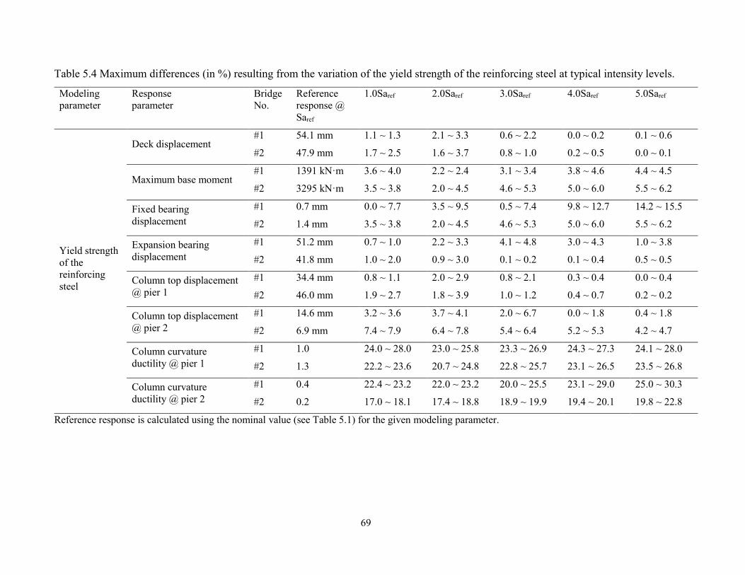
69

Table 5.4 Maximum differences (in %) resulting from the variation of the yield strength of the reinforcing steel at typical intensity levels.


Modeling

parameter

Response

parameter

Bridge

No.

Reference

response @

Saref


Yield strength

of the

reinforcing

steel


#2 47.9 mm 1.7 ~ 2.5 1.6 ~ 3.7 0.8 ~ 1.0 0.2 ~ 0.5 0.0 ~ 0.1


#2 3295 kN·m 3.5 ~ 3.8 2.0 ~ 4.5 4.6 ~ 5.3 5.0 ~ 6.0 5.5 ~ 6.2

Fixed bearing

displacement

#1 0.7 mm 0.0 ~ 7.7 3.5 ~ 9.5 0.5 ~ 7.4 9.8 ~ 12.7 14.2 ~ 15.5

#2 1.4 mm 3.5 ~ 3.8 2.0 ~ 4.5 4.6 ~ 5.3 5.0 ~ 6.0 5.5 ~ 6.2

Expansion bearing

displacement

#1 51.2 mm 0.7 ~ 1.0 2.2 ~ 3.3 4.1 ~ 4.8 3.0 ~ 4.3 1.0 ~ 3.8

#2 41.8 mm 1.0 ~ 2.0 0.9 ~ 3.0 0.1 ~ 0.2 0.1 ~ 0.4 0.5 ~ 0.5


@ pier 1

#1 34.4 mm 0.8 ~ 1.1 2.0 ~ 2.9 0.8 ~ 2.1 0.3 ~ 0.4 0.0 ~ 0.4

#2 46.0 mm 1.9 ~ 2.7 1.8 ~ 3.9 1.0 ~ 1.2 0.4 ~ 0.7 0.2 ~ 0.2


@ pier 2

#1 14.6 mm 3.2 ~ 3.6 3.7 ~ 4.1 2.0 ~ 6.7 0.0 ~ 1.8 0.4 ~ 1.8

#2 6.9 mm 7.4 ~ 7.9 6.4 ~ 7.8 5.4 ~ 6.4 5.2 ~ 5.3 4.2 ~ 4.7

Column curvature

ductility @ pier 1

#1 1.0 24.0 ~ 28.0 23.0 ~ 25.8 23.3 ~ 26.9 24.3 ~ 27.3 24.1 ~ 28.0

#2 1.3 22.2 ~ 23.6 20.7 ~ 24.8 22.8 ~ 25.7 23.1 ~ 26.5 23.5 ~ 26.8

Column curvature

ductility @ pier 2

#1 0.4 22.4 ~ 23.2 22.0 ~ 23.2 20.0 ~ 25.5 23.1 ~ 29.0 25.0 ~ 30.3

#2 0.2 17.0 ~ 18.1 17.4 ~ 18.8 18.9 ~ 19.9 19.4 ~ 20.1 19.8 ~ 22.8

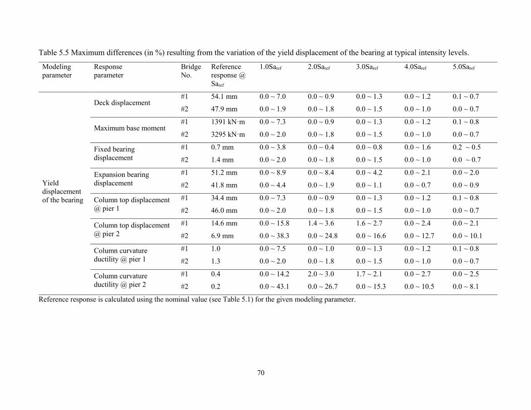
70

Table 5.5 Maximum differences (in %) resulting from the variation of the yield displacement of the bearing at typical intensity levels.


Modeling

parameter

Response

parameter

Bridge

No.

Reference

response @

Saref


Yield

displacement

of the bearing


#2 47.9 mm 0.0 ~ 1.9 0.0 ~ 1.8 0.0 ~ 1.5 0.0 ~ 1.0 0.0 ~ 0.7


#2 3295 kN·m 0.0 ~ 2.0 0.0 ~ 1.8 0.0 ~ 1.5 0.0 ~ 1.0 0.0 ~ 0.7

Fixed bearing

displacement

#1 0.7 mm 0.0 ~ 3.8 0.0 ~ 0.4 0.0 ~ 0.8 0.0 ~ 1.6 0.2 ~ 0.5

#2 1.4 mm 0.0 ~ 2.0 0.0 ~ 1.8 0.0 ~ 1.5 0.0 ~ 1.0 0.0 ~ 0.7

Expansion bearing

displacement

#1 51.2 mm 0.0 ~ 8.9 0.0 ~ 8.4 0.0 ~ 4.2 0.0 ~ 2.1 0.0 ~ 2.0

#2 41.8 mm 0.0 ~ 4.4 0.0 ~ 1.9 0.0 ~ 1.1 0.0 ~ 0.7 0.0 ~ 0.9


@ pier 1

#1 34.4 mm 0.0 ~ 7.3 0.0 ~ 0.9 0.0 ~ 1.3 0.0 ~ 1.2 0.1 ~ 0.8

#2 46.0 mm 0.0 ~ 2.0 0.0 ~ 1.8 0.0 ~ 1.5 0.0 ~ 1.0 0.0 ~ 0.7


@ pier 2

#1 14.6 mm 0.0 ~ 15.8 1.4 ~ 3.6 1.6 ~ 2.7 0.0 ~ 2.4 0.0 ~ 2.1

#2 6.9 mm 0.0 ~ 38.3 0.0 ~ 24.8 0.0 ~ 16.6 0.0 ~ 12.7 0.0 ~ 10.1

Column curvature

ductility @ pier 1

#1 1.0 0.0 ~ 7.5 0.0 ~ 1.0 0.0 ~ 1.3 0.0 ~ 1.2 0.1 ~ 0.8

#2 1.3 0.0 ~ 2.0 0.0 ~ 1.8 0.0 ~ 1.5 0.0 ~ 1.0 0.0 ~ 0.7

Column curvature

ductility @ pier 2

#1 0.4 0.0 ~ 14.2 2.0 ~ 3.0 1.7 ~ 2.1 0.0 ~ 2.7 0.0 ~ 2.5

#2 0.2 0.0 ~ 43.1 0.0 ~ 26.7 0.0 ~ 15.3 0.0 ~ 10.5 0.0 ~ 8.1

71

Table 5.6 Maximum differences (in %) resulting from the variation of the post-yield stiffness of the bearing at typical intensity levels.


Modeling

parameter

Response

parameter

Bridge

No.

Reference

response @

Saref


Post-yield

stiffness of the

bearing


#2 47.9 mm 0.5 ~ 1.7 1.6 ~ 2.7 2.6 ~ 5.1 2.4 ~ 6.2 3.0 ~ 7.3


#2 3295 kN·m 0.5 ~ 1.6 1.6 ~ 2.7 2.5 ~ 5.1 2.4 ~ 6.2 3.0 ~ 7.2

Fixed bearing

displacement

#1 0.7 mm 0.4 ~ 2.4 0.4 ~ 1.0 1.4 ~ 3.0 3.6 ~ 6.0 3.8 ~ 6.6

#2 1.4 mm 0.6 ~ 1.6 1.5 ~ 2.7 2.5 ~ 5.0 2.4 ~ 6.1 3.0 ~ 7.2

Expansion bearing

displacement

#1 51.2 mm 15.6 ~ 17.1 17.0 ~ 20.6 16.9 ~ 22.9 18.9 ~ 29.9 20.4 ~ 36.7

#2 41.8 mm 11.1 ~ 12.0 11.5 ~ 15.2 12.8 ~ 17.5 12.9 ~ 18.9 15.2 ~ 20.4


@ pier 1

#1 34.4 mm 0.0 ~ 1.9 0.2 ~ 1.1 1.8 ~ 3.7 3.5 ~ 5.5 4.2 ~ 6.2

#2 46.0 mm 0.5 ~ 1.6 1.6 ~ 2.7 2.5 ~ 5.1 2.4 ~ 6.2 3.0 ~ 7.2


@ pier 2

#1 14.6 mm 4.9 ~ 11.9 3.0 ~ 23.0 2.8 ~ 30.6 1.6 ~ 36.1 1.0 ~ 35.6

#2 6.9 mm 48.2 ~ 59.0 52.5 ~ 63.5 57.4 ~ 65.2 59.4 ~ 69.7 60.4 ~ 83.0

Column curvature

ductility @ pier 1

#1 1.0 0.1 ~ 1.9 0.2 ~ 1.1 1.9 ~ 3.7 3.5 ~ 5.4 4.1 ~ 6.2

#2 1.3 0.5 ~ 1.6 1.6 ~ 2.7 2.5 ~ 5.1 2.4 ~ 6.2 3.0 ~ 7.2

Column curvature

ductility @ pier 2

#1 0.4 6.4 ~ 13.3 4.4 ~ 25.9 4.0 ~ 34.2 2.6 ~ 40.4 1.8 ~ 39.8

#2 0.2 39.3 ~ 66.9 43.3 ~ 71.5 48.0 ~ 69.7 50.7 ~ 73.3 51.8 ~ 89.3

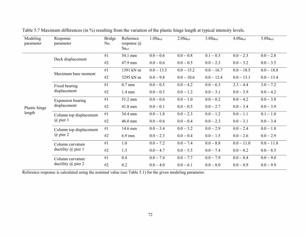
72

Table 5.7 Maximum differences (in %) resulting from the variation of the plastic hinge length at typical intensity levels.


Modeling

parameter

Response

parameter

Bridge

No.

Reference

response @

Saref


Plastic hinge

length


#2 47.9 mm 0.0 ~ 0.6 0.0 ~ 0.5 0.0 ~ 2.3 0.0 ~ 3.2 0.0 ~ 3.5


#2 3295 kN·m 0.0 ~ 9.8 0.0 ~ 10.6 0.0 ~ 12.4 0.0 ~ 13.1 0.0 ~ 13.4

Fixed bearing

displacement

#1 0.7 mm 0.0 ~ 0.5 0.0 ~ 4.2 0.0 ~ 6.3 2.3 ~ 4.4 3.0 ~ 7.2

#2 1.4 mm 0.0 ~ 0.3 0.0 ~ 1.2 0.0 ~ 3.1 0.0 ~ 3.9 0.0 ~ 4.2

Expansion bearing

displacement

#1 51.2 mm 0.0 ~ 0.6 0.0 ~ 1.0 0.0 ~ 0.2 0.0 ~ 4.2 0.0 ~ 3.8

#2 41.8 mm 0.0 ~ 0.1 0.0 ~ 0.5 0.0 ~ 2.7 0.0 ~ 3.4 0.0 ~ 3.9


@ pier 1

#1 34.4 mm 0.0 ~ 1.8 0.0 ~ 2.3 0.0 ~ 1.2 0.0 ~ 1.1 0.1 ~ 1.8

#2 46.0 mm 0.0 ~ 0.6 0.0 ~ 0.4 0.0 ~ 2.3 0.0 ~ 3.1 0.0 ~ 3.4


@ pier 2

#1 14.6 mm 0.0 ~ 3.4 0.0 ~ 3.2 0.0 ~ 2.9 0.0 ~ 2.4 0.0 ~ 1.8

#2 6.9 mm 0.0 ~ 2.3 0.0 ~ 0.4 0.0 ~ 1.5 0.0 ~ 2.6 0.0 ~ 2.9

Column curvature

ductility @ pier 1

#1 1.0 0.0 ~ 7.2 0.0 ~ 7.4 0.0 ~ 8.8 0.0 ~ 11.0 0.0 ~ 11.8

#2 1.3 0.0 ~ 4.7 0.0 ~ 5.5 0.0 ~ 7.4 0.0 ~ 8.2 0.0 ~ 8.5

Column curvature

ductility @ pier 2

#1 0.4 0.0 ~ 7.4 0.0 ~ 7.7 0.0 ~ 7.9 0.0 ~ 8.4 0.0 ~ 9.0

#2 0.2 0.0 ~ 4.0 0.0 ~ 6.1 0.0 ~ 8.0 0.0 ~ 8.9 0.0 ~ 9.9

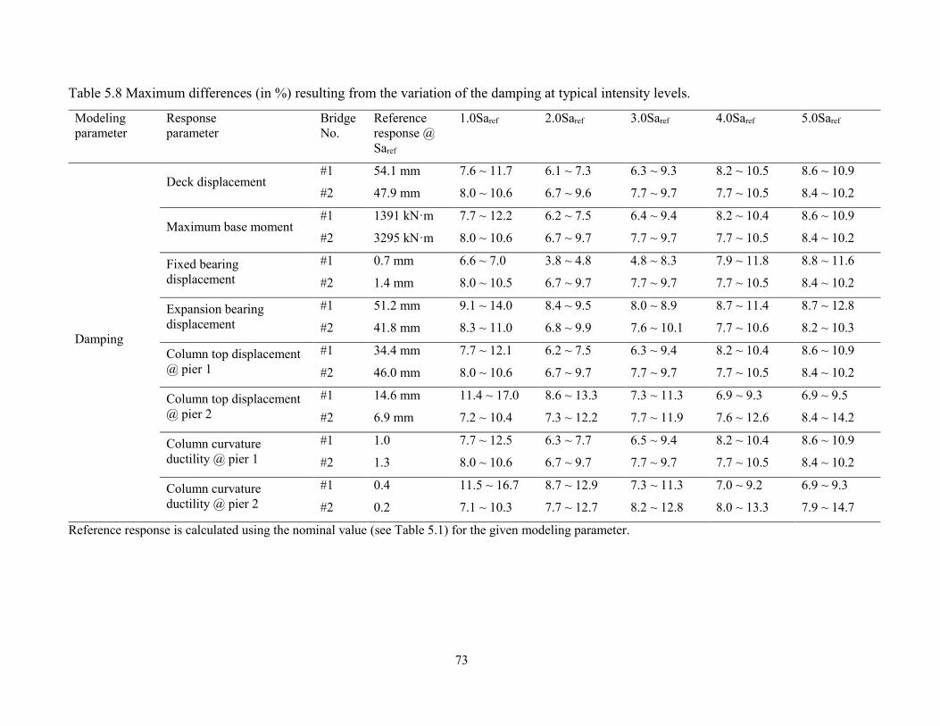
73

Table 5.8 Maximum differences (in %) resulting from the variation of the damping at typical intensity levels.


Modeling

parameter

Response

parameter

Bridge

No.

Reference

response @

Saref


Damping


#2 47.9 mm 8.0 ~ 10.6 6.7 ~ 9.6 7.7 ~ 9.7 7.7 ~ 10.5 8.4 ~ 10.2


#2 3295 kN·m 8.0 ~ 10.6 6.7 ~ 9.7 7.7 ~ 9.7 7.7 ~ 10.5 8.4 ~ 10.2

Fixed bearing

displacement

#1 0.7 mm 6.6 ~ 7.0 3.8 ~ 4.8 4.8 ~ 8.3 7.9 ~ 11.8 8.8 ~ 11.6

#2 1.4 mm 8.0 ~ 10.5 6.7 ~ 9.7 7.7 ~ 9.7 7.7 ~ 10.5 8.4 ~ 10.2

Expansion bearing

displacement

#1 51.2 mm 9.1 ~ 14.0 8.4 ~ 9.5 8.0 ~ 8.9 8.7 ~ 11.4 8.7 ~ 12.8

#2 41.8 mm 8.3 ~ 11.0 6.8 ~ 9.9 7.6 ~ 10.1 7.7 ~ 10.6 8.2 ~ 10.3


@ pier 1

#1 34.4 mm 7.7 ~ 12.1 6.2 ~ 7.5 6.3 ~ 9.4 8.2 ~ 10.4 8.6 ~ 10.9

#2 46.0 mm 8.0 ~ 10.6 6.7 ~ 9.7 7.7 ~ 9.7 7.7 ~ 10.5 8.4 ~ 10.2


@ pier 2

#1 14.6 mm 11.4 ~ 17.0 8.6 ~ 13.3 7.3 ~ 11.3 6.9 ~ 9.3 6.9 ~ 9.5

#2 6.9 mm 7.2 ~ 10.4 7.3 ~ 12.2 7.7 ~ 11.9 7.6 ~ 12.6 8.4 ~ 14.2

Column curvature

ductility @ pier 1

#1 1.0 7.7 ~ 12.5 6.3 ~ 7.7 6.5 ~ 9.4 8.2 ~ 10.4 8.6 ~ 10.9

#2 1.3 8.0 ~ 10.6 6.7 ~ 9.7 7.7 ~ 9.7 7.7 ~ 10.5 8.4 ~ 10.2

Column curvature

ductility @ pier 2

#1 0.4 11.5 ~ 16.7 8.7 ~ 12.9 7.3 ~ 11.3 7.0 ~ 9.2 6.9 ~ 9.3

#2 0.2 7.1 ~ 10.3 7.7 ~ 12.7 8.2 ~ 12.8 8.0 ~ 13.3 7.9 ~ 14.7

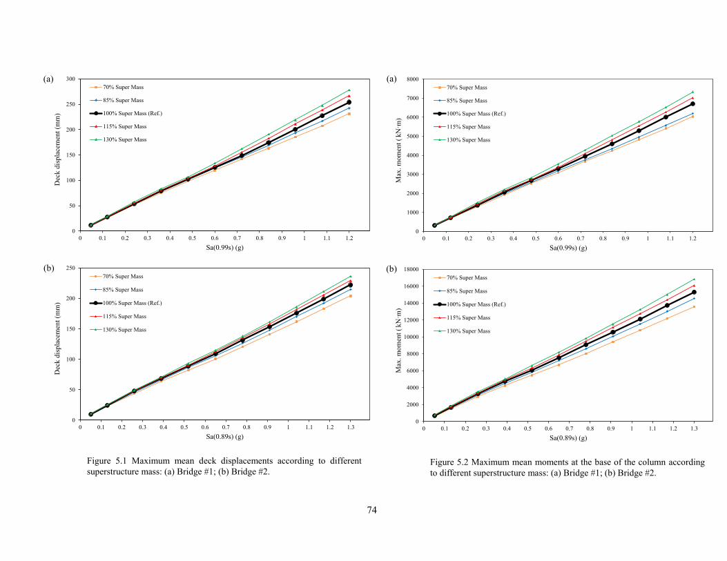
74

.

0

50

100

150

200

250

300

0 0.1 0.2 0.3 0.4 0.5 0.6 0.7 0.8 0.9 1 1.1 1.2

Dec

k d

isp

lace

men

t (m

m)

Sa(0.99s) (g)

70% Super Mass

85% Super Mass

100% Super Mass (Ref.)

115% Super Mass

130% Super Mass

0

50

100

150

200

250

0 0.1 0.2 0.3 0.4 0.5 0.6 0.7 0.8 0.9 1 1.1 1.2 1.3

Dec

k d

isp

lace

men

t (m

m)

Sa(0.89s) (g)

70% Super Mass

85% Super Mass


115% Super Mass

130% Super Mass

(b)

(a)

Figure 5.1 Maximum mean deck displacements according to different

superstructure mass: (a) Bridge #1; (b) Bridge #2.

0

1000

2000

3000

4000

5000

6000

7000

8000

0 0.1 0.2 0.3 0.4 0.5 0.6 0.7 0.8 0.9 1 1.1 1.2

Max

. m

om

ent

(k

N·m

)

Sa(0.99s) (g)

70% Super Mass

85% Super Mass


115% Super Mass

130% Super Mass

0

2000

4000

6000

8000

10000

12000

14000

16000

18000

0 0.1 0.2 0.3 0.4 0.5 0.6 0.7 0.8 0.9 1 1.1 1.2 1.3

Max

. m

om

ent

(k

N·m

)

Sa(0.89s) (g)

70% Super Mass

85% Super Mass


115% Super Mass

130% Super Mass

(a)

(b)

Figure 5.2 Maximum mean moments at the base of the column according

to different superstructure mass: (a) Bridge #1; (b) Bridge #2.

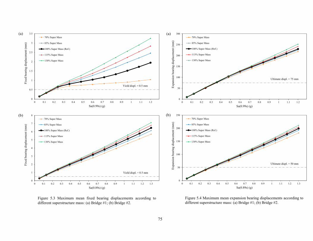
75

0

0.5

1

1.5

2

2.5

3

3.5

0 0.1 0.2 0.3 0.4 0.5 0.6 0.7 0.8 0.9 1 1.1 1.2

Fix

ed b

eari

ng d

isp

lace

men

t (m

m)

Sa(0.99s) (g)

70% Super Mass

85% Super Mass


115% Super Mass

130% Super Mass

Yield displ. = 0.5 mm

0

1

2

3

4

5

6

7

8

0 0.1 0.2 0.3 0.4 0.5 0.6 0.7 0.8 0.9 1 1.1 1.2 1.3

Fix

ed b

eari

ng d

isp

lace

men

t (m

m)

Sa(0.89s) (g)

70% Super Mass

85% Super Mass


115% Super Mass

130% Super Mass


(a)

(b)

Figure 5.3 Maximum mean fixed bearing displacements according to

different superstructure mass: (a) Bridge #1; (b) Bridge #2.

0

50

100

150

200

250

300

0 0.1 0.2 0.3 0.4 0.5 0.6 0.7 0.8 0.9 1 1.1 1.2

Ex

pan

sio

n b

eari

ng d

isp

lace

men

t (m

m)

Sa(0.99s) (g)

70% Super Mass

85% Super Mass


115% Super Mass

130% Super Mass

Ultimate displ. = 75 mm

0

50

100

150

200

250

0 0.1 0.2 0.3 0.4 0.5 0.6 0.7 0.8 0.9 1 1.1 1.2 1.3

Ex

pan

sio

n b

eari

ng d

isp

lace

men

t (m

m)

Sa(0.89s) (g)

70% Super Mass

85% Super Mass


115% Super Mass

130% Super Mass


(b)

(a)

Figure 5.4 Maximum mean expansion bearing displacements according to

different superstructure mass: (a) Bridge #1; (b) Bridge #2.

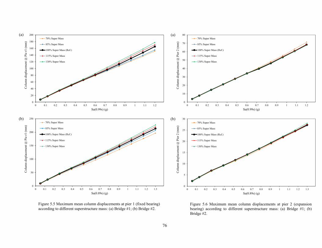
76

0

20

40

60

80

100

120

140

160

180

200

0 0.1 0.2 0.3 0.4 0.5 0.6 0.7 0.8 0.9 1 1.1 1.2

Co

lum

n d

isp

lace

men

t @

Pie

r1

(m

m)

Sa(0.99s) (g)

70% Super Mass

85% Super Mass


115% Super Mass

130% Super Mass

0

50

100

150

200

250

0 0.1 0.2 0.3 0.4 0.5 0.6 0.7 0.8 0.9 1 1.1 1.2 1.3

Co

lum

n d

isp

lace

men

t @

Pie

r1

(m

m)

Sa(0.89s) (g)

70% Super Mass

85% Super Mass


115% Super Mass

130% Super Mass

(a)

(b)

Figure 5.5 Maximum mean column displacements at pier 1 (fixed bearing)

according to different superstructure mass: (a) Bridge #1; (b) Bridge #2.

0

10

20

30

40

50

60

70

80

0 0.1 0.2 0.3 0.4 0.5 0.6 0.7 0.8 0.9 1 1.1 1.2

Co

lum

n d

isp

lace

men

t @

Pie

r 2

(m

m)

Sa(0.99s) (g)

70% Super Mass

85% Super Mass


115% Super Mass

130% Super Mass

0

5

10

15

20

25

30

0 0.1 0.2 0.3 0.4 0.5 0.6 0.7 0.8 0.9 1 1.1 1.2 1.3

Co

lum

n d

isp

lace

men

t @

Pie

r 2

(m

m)

Sa(0.89s) (g)

70% Super Mass

85% Super Mass


115% Super Mass

130% Super Mass

(a)

(b)

Figure 5.6 Maximum mean column displacements at pier 2 (expansion

bearing) according to different superstructure mass: (a) Bridge #1; (b)

Bridge #2.

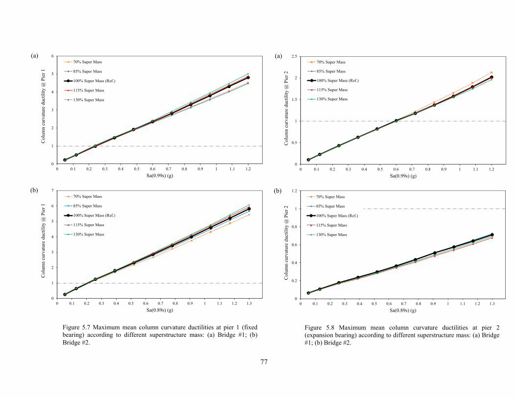
77

0

1

2

3

4

5

6

0 0.1 0.2 0.3 0.4 0.5 0.6 0.7 0.8 0.9 1 1.1 1.2

Co

lum

n c

urv

atu

re d

uct

ilit

y @

Pie

r 1

Sa(0.99s) (g)

70% Super Mass

85% Super Mass


115% Super Mass

130% Super Mass

0

1

2

3

4

5

6

7

0 0.1 0.2 0.3 0.4 0.5 0.6 0.7 0.8 0.9 1 1.1 1.2 1.3

Co

lum

n c

urv

atu

re d

uct

ilit

y @

Pie

r 1

Sa(0.89s) (g)

70% Super Mass

85% Super Mass


115% Super Mass

130% Super Mass

(a)

(b)

Figure 5.7 Maximum mean column curvature ductilities at pier 1 (fixed

bearing) according to different superstructure mass: (a) Bridge #1; (b)

Bridge #2.

0

0.5

1

1.5

2

2.5

0 0.1 0.2 0.3 0.4 0.5 0.6 0.7 0.8 0.9 1 1.1 1.2

Co

lum

n c

urv

atu

re d

uct

ilit

y @

Pie

r 2

Sa(0.99s) (g)

70% Super Mass

85% Super Mass


115% Super Mass

130% Super Mass

0

0.2

0.4

0.6

0.8

1

1.2

0 0.1 0.2 0.3 0.4 0.5 0.6 0.7 0.8 0.9 1 1.1 1.2 1.3

Co

lum

n c

urv

atu

re d

uct

ilit

y @

Pie

r 2

Sa(0.89s) (g)

70% Super Mass

85% Super Mass


115% Super Mass

130% Super Mass

(a)

(b)

Figure 5.8 Maximum mean column curvature ductilities at pier 2

(expansion bearing) according to different superstructure mass: (a) Bridge

#1; (b) Bridge #2.

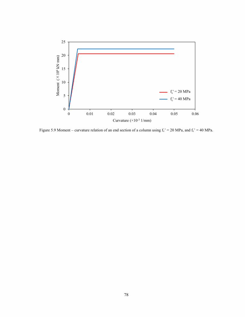
78

Figure 5.9 Moment – curvature relation of an end section of a column using fc’ = 20 MPa, and fc’ = 40 MPa.

0

5

10

15

20

25

0 0.01 0.02 0.03 0.04 0.05 0.06

Mo

men

t (×

10

6kN

·mm

)

Curvature ( 10-3 1/mm)

f'c = 20MPa

f'c = 40MPa

fc' = 20 MPa

fc' = 40 MPa

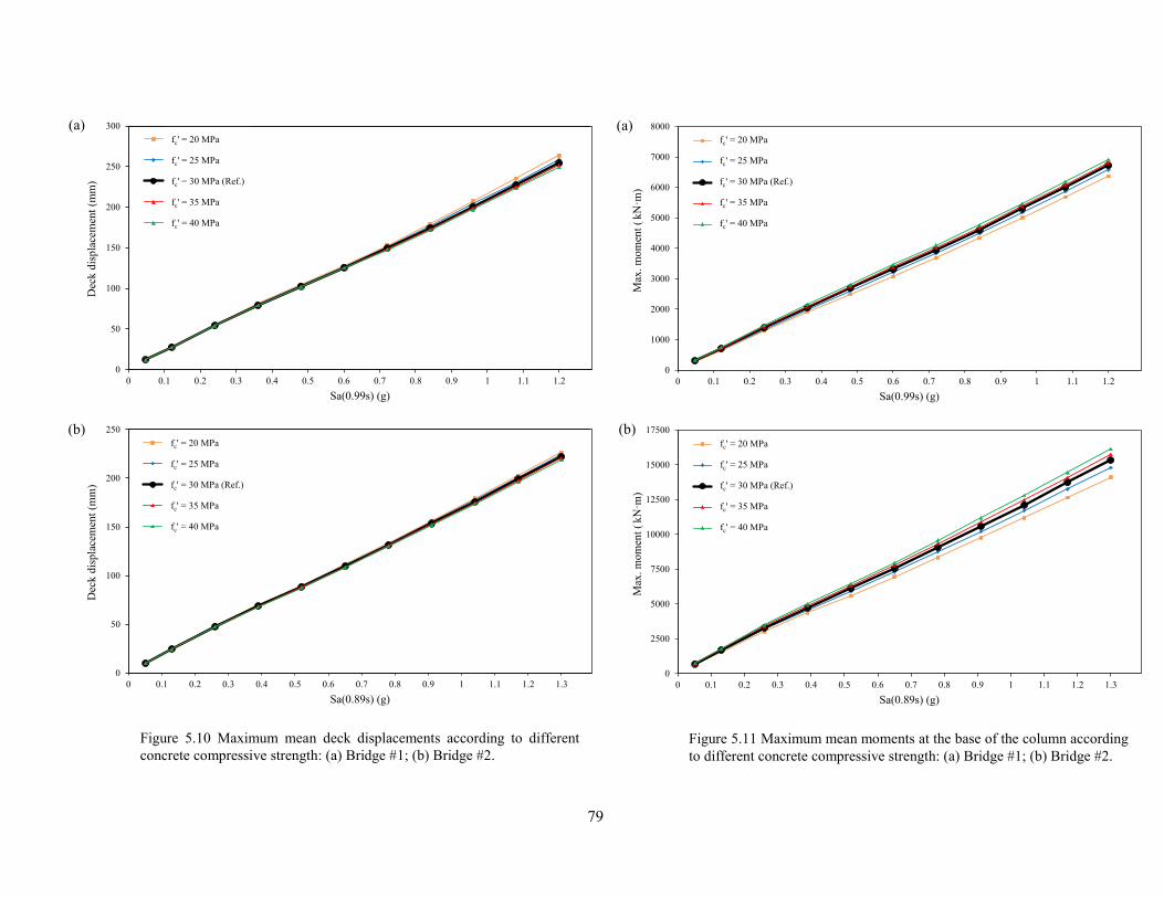
79

0

1000

2000

3000

4000

5000

6000

7000

8000

0 0.1 0.2 0.3 0.4 0.5 0.6 0.7 0.8 0.9 1 1.1 1.2

Max

. m

om

ent

(k

N·m

)

Sa(0.99s) (g)

f'c = 20 Mpa

f'c = 25 Mpa

f'c = 30 Mpa (Ref.)

f'c = 35 Mpa

f'c = 40 Mpa

fc' = 20 MPa

fc' = 25 MPa

fc' = 30 MPa (Ref.)

fc' = 35 MPa

fc' = 40 MPa

0

2500

5000

7500

10000

12500

15000

17500

0 0.1 0.2 0.3 0.4 0.5 0.6 0.7 0.8 0.9 1 1.1 1.2 1.3

Max

. m

om

ent

(k

N·m

)

Sa(0.89s) (g)

f'c = 20MPa

f'c = 25MPa

f'c = 30MPa (Ref.)

f'c = 35MPa

f'c = 40MPa

fc' = 20 MPa

fc' = 25 MPa

fc' = 30 MPa (Ref.)

fc' = 35 MPa

fc' = 40 MPa

(a)

(b)


to different concrete compressive strength: (a) Bridge #1; (b) Bridge #2.

0

50

100

150

200

250

300

0 0.1 0.2 0.3 0.4 0.5 0.6 0.7 0.8 0.9 1 1.1 1.2

Dec

k d

isp

lace

men

t (m

m)

Sa(0.99s) (g)

f'c = 20 Mpa

f'c = 25 Mpa

f'c = 30 MPa (Ref.)

f'c = 35 Mpa

f'c = 40 Mpa

fc' = 20 MPa

fc' = 25 MPa

fc' = 30 MPa (Ref.)

fc' = 35 MPa

fc' = 40 MPa

0

50

100

150

200

250

0 0.1 0.2 0.3 0.4 0.5 0.6 0.7 0.8 0.9 1 1.1 1.2 1.3

Dec

k d

isp

lace

men

t (m

m)

Sa(0.89s) (g)

f'c = 20MPa

f'c = 25MPa

f'c = 30MPa (Ref.)

f'c = 35MPa

f'c = 40MPa

fc' = 20 MPa

fc' = 25 MPa

fc' = 30 MPa (Ref.)

fc' = 35 MPa

fc' = 40 MPa


concrete compressive strength: (a) Bridge #1; (b) Bridge #2.

(a)

(b)

80

0

50

100

150

200

250

0 0.1 0.2 0.3 0.4 0.5 0.6 0.7 0.8 0.9 1 1.1 1.2

Ex

pan

sion

bea

ring d

ispla

cem

ent

(mm

)

Sa(0.99s) (g)

f'c = 20 Mpa

f'c = 25 Mpa

f'c = 30 Mpa (Ref.)

f'c = 35 Mpa

f'c = 40 Mpa

fc' = 20 MPa

fc' = 25 MPa

fc' = 30 MPa (Ref.)

fc' = 35 MPa

fc' = 40 MPa


0

50

100

150

200

250

0 0.1 0.2 0.3 0.4 0.5 0.6 0.7 0.8 0.9 1 1.1 1.2 1.3

Ex

pan

sion

bea

ring d

ispla

cem

ent

(mm

)

Sa(0.89s) (g)

f'c = 20MPa

f'c = 25MPa

f'c = 30MPa (Ref.)

f'c = 35MPa

f'c = 40MPa

fc' = 20 MPa

fc' = 25 MPa

fc' = 30 MPa (Ref.)

fc' = 35 MPa

fc' = 40 MPa


(a)

(b)


different concrete compressive strength: (a) Bridge #1; (b) Bridge #2.

0

0.5

1

1.5

2

2.5

0 0.1 0.2 0.3 0.4 0.5 0.6 0.7 0.8 0.9 1 1.1 1.2

Fix

ed b

eari

ng d

isp

lace

men

t (m

m)

Sa(0.99s) (g)

f'c = 20 Mpa

f'c = 25 Mpa

f'c = 30 Mpa (Ref.)

f'c = 35 Mpa

f'c = 40 Mpa

fc' = 20 MPa

fc' = 25 MPa

fc' = 30 MPa (Ref.)

fc' = 35 MPa

fc' = 40 MPa


0

1

2

3

4

5

6

7

8

0 0.1 0.2 0.3 0.4 0.5 0.6 0.7 0.8 0.9 1 1.1 1.2 1.3

Fix

ed b

eari

ng d

isp

lace

men

t (m

m)

Sa(0.89s) (g)

f'c = 20MPa

f'c = 25MPa

f'c = 30MPa (Ref.)

f'c = 35MPa

f'c = 40MPa

fc' = 20 MPa

fc' = 25 MPa

fc' = 30 MPa (Ref.)

fc' = 35 MPa

fc' = 40 MPa


(a)

(b)


different concrete compressive strength: (a) Bridge #1; (b) Bridge #2.

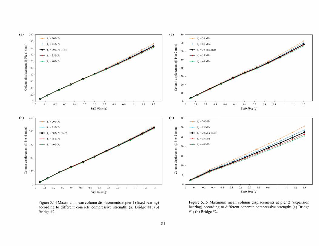
81

0

20

40

60

80

100

120

140

160

180

200

0 0.1 0.2 0.3 0.4 0.5 0.6 0.7 0.8 0.9 1 1.1 1.2

Co

lum

n d

isp

lace

men

t @

Pie

r1

(m

m)

Sa(0.99s) (g)

f'c = 20 Mpa

f'c = 25 Mpa

f'c = 30 Mpa (Ref.)

f'c = 35 Mpa

f'c = 40 Mpa

fc' = 20 MPa

fc' = 25 MPa

fc' = 30 MPa (Ref.)

fc' = 35 MPa

fc' = 40 MPa

0

50

100

150

200

250

0 0.1 0.2 0.3 0.4 0.5 0.6 0.7 0.8 0.9 1 1.1 1.2 1.3

Co

lum

n d

isp

lace

men

t @

Pie

r1

(m

m)

Sa(0.89s) (g)

f'c = 20MPa

f'c = 25MPa

f'c = 30MPa (Ref.)

f'c = 35MPa

f'c = 40MPa

fc' = 20 MPa

fc' = 25 MPa

fc' = 30 MPa (Ref.)

fc' = 35 MPa

fc' = 40 MPa


according to different concrete compressive strength: (a) Bridge #1; (b)

Bridge #2.

(a)

(b)

0

10

20

30

40

50

60

70

80

0 0.1 0.2 0.3 0.4 0.5 0.6 0.7 0.8 0.9 1 1.1 1.2

Co

lum

n d

isp

lace

men

t @

Pie

r 2

(m

m)

Sa(0.99s) (g)

f'c = 20 Mpa

f'c = 25 Mpa

f'c = 30 Mpa (Ref.)

f'c = 35 Mpa

f'c = 40 Mpa

fc' = 20 MPa

fc' = 25 MPa

fc' = 30 MPa (Ref.)

fc' = 35 MPa

fc' = 40 MPa

0

5

10

15

20

25

30

35

0 0.1 0.2 0.3 0.4 0.5 0.6 0.7 0.8 0.9 1 1.1 1.2 1.3

Co

lum

n d

isp

lace

men

t @

Pie

r 2

(m

m)

Sa(0.89s) (g)

f'c = 20MPa

f'c = 25MPa

f'c = 30MPa (Ref.)

f'c = 35MPa

f'c = 40MPa

fc' = 20 MPa

fc' = 25 MPa

fc' = 30 MPa (Ref.)

fc' = 35 MPa

fc' = 40 MPa


bearing) according to different concrete compressive strength: (a) Bridge

#1; (b) Bridge #2.

(a)

(b)

82

0

1

2

3

4

5

6

0 0.1 0.2 0.3 0.4 0.5 0.6 0.7 0.8 0.9 1 1.1 1.2

Co

lum

n c

urv

atu

re d

uct

ilit

y @

Pie

r 1

Sa(0.99s) (g)

f'c = 20 Mpa

f'c = 25 Mpa

f'c = 30 Mpa (Ref.)

f'c = 35 Mpa

f'c = 40 Mpa

fc' = 20 MPa

fc' = 25 MPa

fc' = 30 MPa (Ref.)

fc' = 35 MPa

fc' = 40 MPa

0

1

2

3

4

5

6

7

0 0.1 0.2 0.3 0.4 0.5 0.6 0.7 0.8 0.9 1 1.1 1.2 1.3

Co

lum

n c

urv

atu

re d

uct

ilit

y @

Pie

r 1

Sa(0.89s) (g)

f'c = 20MPa

f'c = 25MPa

f'c = 30MPa (Ref.)

f'c = 35MPa

f'c = 40MPa

fc' = 20 MPa

fc' = 25 MPa

fc' = 30 MPa (Ref.)

fc' = 35 MPa

fc' = 40 MPa


bearing) according to different concrete compressive strength: (a) Bridge

#1; (b) Bridge #2.

(a)

(b)

0

0.5

1

1.5

2

2.5

0 0.1 0.2 0.3 0.4 0.5 0.6 0.7 0.8 0.9 1 1.1 1.2

Co

lum

n c

urv

atu

re d

uct

ilit

y @

Pie

r 2

Sa(0.99s) (g)

f'c = 20 Mpa

f'c = 25 Mpa

f'c = 30 Mpa (Ref.)

f'c = 35 Mpa

f'c = 40 Mpa

fc' = 20 MPa

fc' = 25 MPa

fc' = 30 MPa (Ref.)

fc' = 35 MPa

fc' = 40 MPa

0

0.2

0.4

0.6

0.8

1

1.2

0 0.1 0.2 0.3 0.4 0.5 0.6 0.7 0.8 0.9 1 1.1 1.2 1.3

Co

lum

n c

urv

atu

re d

uct

ilit

y @

Pie

r 2

Sa(0.89s) (g)

f'c = 20MPa

f'c = 25MPa

f'c = 30MPa (Ref.)

f'c = 35MPa

f'c = 40MPa

fc' = 20 MPa

fc' = 25 MPa

fc' = 30 MPa (Ref.)

fc' = 35 MPa

fc' = 40 MPa


(expansion bearing) according to different concrete compressive strength:

(a) Bridge #1; (b) Bridge #2.

(a)

(b)

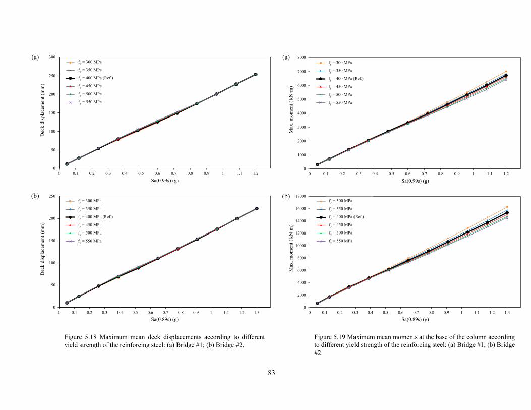
83

0

1000

2000

3000

4000

5000

6000

7000

8000

0 0.1 0.2 0.3 0.4 0.5 0.6 0.7 0.8 0.9 1 1.1 1.2

Max

. m

om

ent

(k

N·m

)

Sa(0.99s) (g)

fy = 300MPa

fy = 350MPa

fy = 400MPa (Ref.)

fy = 450MPa

fy = 500MPa

fy = 550MPa

fy = 300 MPa

fy = 350 MPa

fy = 400 MPa (Ref.)

fy = 450 MPa

fy = 500 MPa

fy = 550 MPa

0

2000

4000

6000

8000

10000

12000

14000

16000

18000

0 0.1 0.2 0.3 0.4 0.5 0.6 0.7 0.8 0.9 1 1.1 1.2 1.3

Max

. m

om

ent

(k

N·m

)

Sa(0.89s) (g)

fy = 300MPa

fy = 350MPa

fy = 400MPa (Ref.)

fy = 450MPa

fy = 500MPa

fy = 550MPa

fy = 300 MPa

fy = 350 MPa

fy = 400 MPa (Ref.)

fy = 450 MPa

fy = 500 MPa

fy = 550 MPa


to different yield strength of the reinforcing steel: (a) Bridge #1; (b) Bridge

#2.

(a)

(b)

0

50

100

150

200

250

300

0 0.1 0.2 0.3 0.4 0.5 0.6 0.7 0.8 0.9 1 1.1 1.2

Dec

k d

isp

lace

men

t (m

m)

Sa(0.99s) (g)

fy = 300MPa

fy = 350MPa

fy = 400MPa (Ref.)

fy = 450MPa

fy = 500MPa

fy = 550MPa

fy = 300 MPa

fy = 350 MPa

fy = 400 MPa (Ref.)

fy = 450 MPa

fy = 500 MPa

fy = 550 MPa

0

50

100

150

200

250

0 0.1 0.2 0.3 0.4 0.5 0.6 0.7 0.8 0.9 1 1.1 1.2 1.3

Dec

k d

isp

lace

men

t (m

m)

Sa(0.89s) (g)

fy = 300MPa

fy = 350MPa

fy = 400MPa (Ref.)

fy = 450MPa

fy = 500MPa

fy = 550MPa

fy = 300 MPa

fy = 350 MPa

fy = 400 MPa (Ref.)

fy = 450 MPa

fy = 500 MPa

fy = 550 MPa

(a)

(b)


yield strength of the reinforcing steel: (a) Bridge #1; (b) Bridge #2.

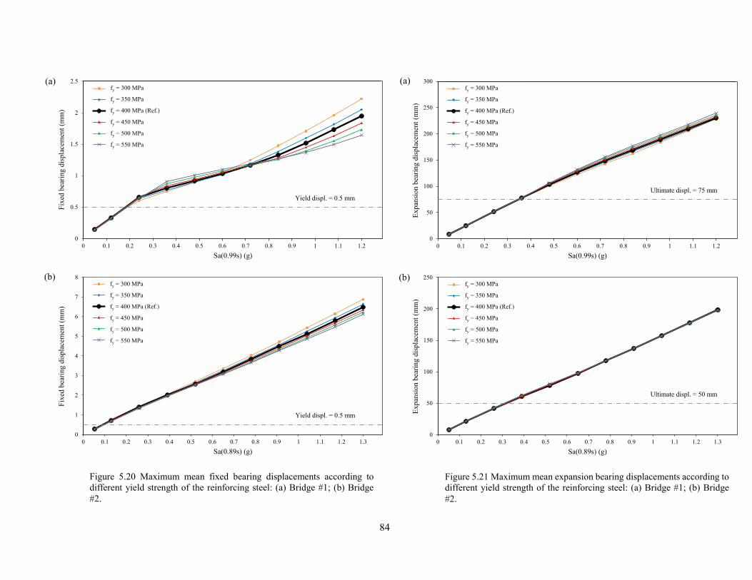
84

0

50

100

150

200

250

300

0 0.1 0.2 0.3 0.4 0.5 0.6 0.7 0.8 0.9 1 1.1 1.2

Ex

pan

sio

n b

eari

ng d

isp

lace

men

t (m

m)

Sa(0.99s) (g)

fy = 300MPa

fy = 350MPa

fy = 400MPa (Ref.)

fy = 450MPa

fy = 500MPa

fy = 550MPa

fy = 300 MPa

fy = 350 MPa

fy = 400 MPa (Ref.)

fy = 450 MPa

fy = 500 MPa

fy = 550 MPa


0

50

100

150

200

250

0 0.1 0.2 0.3 0.4 0.5 0.6 0.7 0.8 0.9 1 1.1 1.2 1.3

Ex

pan

sio

n b

eari

ng d

isp

lace

men

t (m

m)

Sa(0.89s) (g)

fy = 300MPa

fy = 350MPa

fy = 400MPa (Ref.)

fy = 450MPa

fy = 500MPa

fy = 550MPa

fy = 300 MPa

fy = 350 MPa

fy = 400 MPa (Ref.)

fy = 450 MPa

fy = 500 MPa

fy = 550 MPa



different yield strength of the reinforcing steel: (a) Bridge #1; (b) Bridge

#2.

(a)

(b)

0

0.5

1

1.5

2

2.5

0 0.1 0.2 0.3 0.4 0.5 0.6 0.7 0.8 0.9 1 1.1 1.2

Fix

ed b

eari

ng d

isp

lace

men

t (m

m)

Sa(0.99s) (g)

fy = 300MPa

fy = 350MPa

fy = 400MPa (Ref.)

fy = 450MPa

fy = 500MPa

fy = 550MPa

fy = 300 MPa

fy = 350 MPa

fy = 400 MPa (Ref.)

fy = 450 MPa

fy = 500 MPa

fy = 550 MPa


0

1

2

3

4

5

6

7

8

0 0.1 0.2 0.3 0.4 0.5 0.6 0.7 0.8 0.9 1 1.1 1.2 1.3

Fix

ed b

eari

ng d

isp

lace

men

t (m

m)

Sa(0.89s) (g)

fy = 300MPa

fy = 350MPa

fy = 400MPa (Ref.)

fy = 450MPa

fy = 500MPa

fy = 550MPa

fy = 300 MPa

fy = 350 MPa

fy = 400 MPa (Ref.)

fy = 450 MPa

fy = 500 MPa

fy = 550 MPa



different yield strength of the reinforcing steel: (a) Bridge #1; (b) Bridge

#2.

(a)

(b)

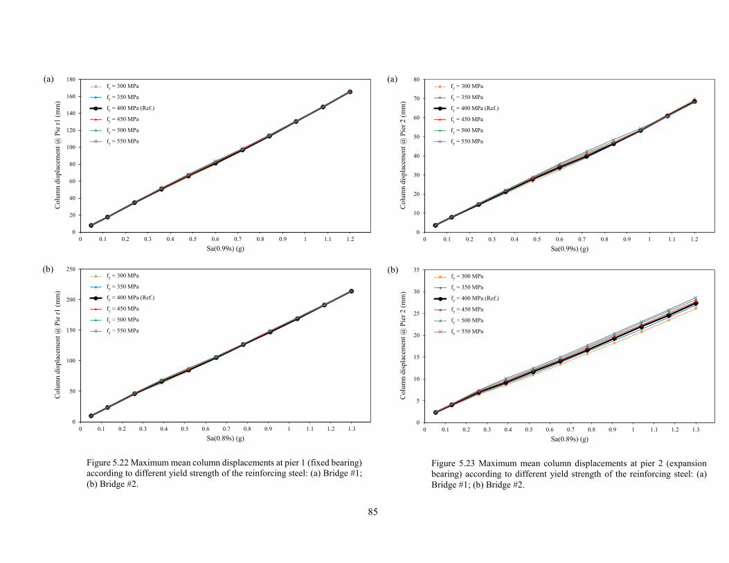
85

0

20

40

60

80

100

120

140

160

180

0 0.1 0.2 0.3 0.4 0.5 0.6 0.7 0.8 0.9 1 1.1 1.2

Co

lum

n d

isp

lace

men

t @

Pie

r1

(m

m)

Sa(0.99s) (g)

fy = 300MPa

fy = 350MPa

fy = 400MPa (Ref.)

fy = 450MPa

fy = 500MPa

fy = 550MPa

fy = 300 MPa

fy = 350 MPa

fy = 400 MPa (Ref.)

fy = 450 MPa

fy = 500 MPa

fy = 550 MPa

0

50

100

150

200

250

0 0.1 0.2 0.3 0.4 0.5 0.6 0.7 0.8 0.9 1 1.1 1.2 1.3

Co

lum

n d

isp

lace

men

t @

Pie

r1

(m

m)

Sa(0.89s) (g)

fy = 300MPa

fy = 350MPa

fy = 400MPa (Ref.)

fy = 450MPa

fy = 500MPa

fy = 550MPa

fy = 300 MPa

fy = 350 MPa

fy = 400 MPa (Ref.)

fy = 450 MPa

fy = 500 MPa

fy = 550 MPa


according to different yield strength of the reinforcing steel: (a) Bridge #1;

(b) Bridge #2.

(a)

(b)

0

10

20

30

40

50

60

70

80

0 0.1 0.2 0.3 0.4 0.5 0.6 0.7 0.8 0.9 1 1.1 1.2

Co

lum

n d

isp

lace

men

t @

Pie

r 2

(m

m)

Sa(0.99s) (g)

fy = 300MPa

fy = 350MPa

fy = 400MPa (Ref.)

fy = 450MPa

fy = 500MPa

fy = 550MPa

fy = 300 MPa

fy = 350 MPa

fy = 400 MPa (Ref.)

fy = 450 MPa

fy = 500 MPa

fy = 550 MPa

0

5

10

15

20

25

30

35

0 0.1 0.2 0.3 0.4 0.5 0.6 0.7 0.8 0.9 1 1.1 1.2 1.3

Co

lum

n d

isp

lace

men

t @

Pie

r 2

(m

m)

Sa(0.89s) (g)

fy = 300MPa

fy = 350MPa

fy = 400MPa (Ref.)

fy = 450MPa

fy = 500MPa

fy = 550MPa

fy = 300 MPa

fy = 350 MPa

fy = 400 MPa (Ref.)

fy = 450 MPa

fy = 500 MPa

fy = 550 MPa


bearing) according to different yield strength of the reinforcing steel: (a)

Bridge #1; (b) Bridge #2.

(a)

(b)

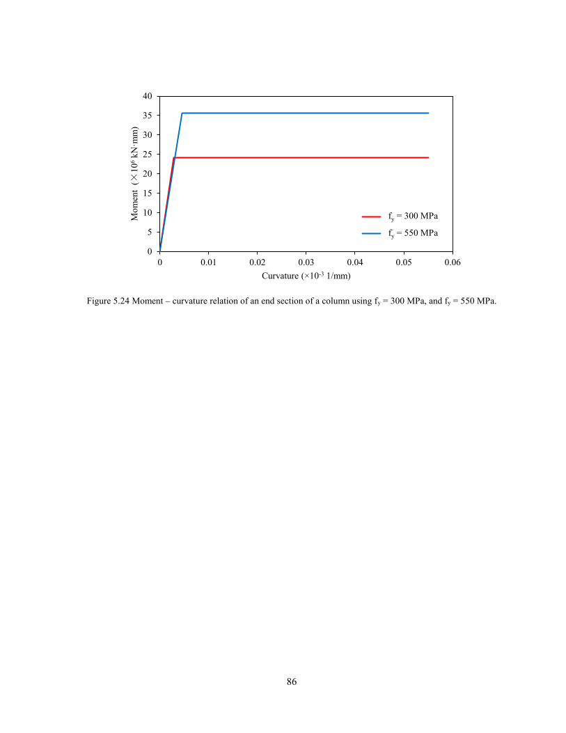
86

Figure 5.24 Moment – curvature relation of an end section of a column using fy = 300 MPa, and fy = 550 MPa.

0

5

10

15

20

25

30

35

40

0 0.01 0.02 0.03 0.04 0.05 0.06

Mo

men

t (×

10

6kN

·mm

)

Curvature ( 10-3 1/mm)

fy = 300MPa

fy = 550MPa

fy = 300 MPa

fy = 550 MPa

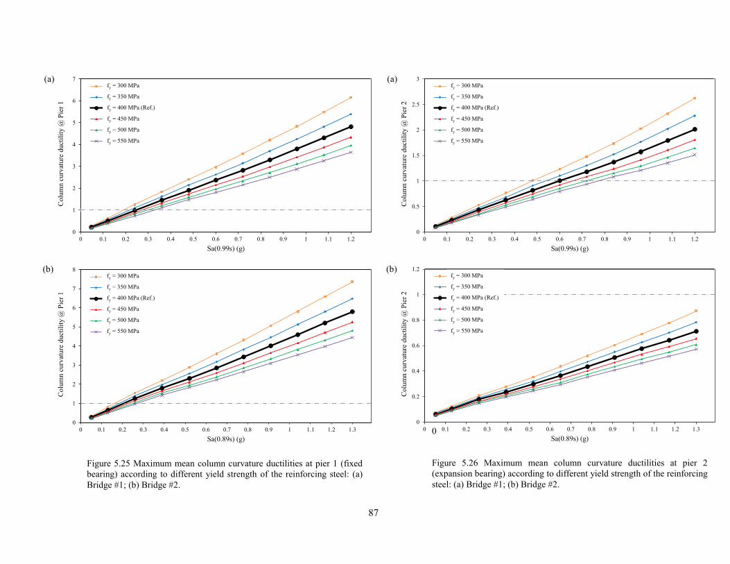
87

0

1

2

3

4

5

6

7

0 0.1 0.2 0.3 0.4 0.5 0.6 0.7 0.8 0.9 1 1.1 1.2

Co

lum

n c

urv

atu

re d

uct

ilit

y @

Pie

r 1

Sa(0.99s) (g)

fy = 300MPa

fy = 350MPa

fy = 400MPa (Ref.)

fy = 450MPa

fy = 500MPa

fy = 550MPa

fy = 300 MPa

fy = 350 MPa

fy = 400 MPa (Ref.)

fy = 450 MPa

fy = 500 MPa

fy = 550 MPa

0

1

2

3

4

5

6

7

8

0 0.1 0.2 0.3 0.4 0.5 0.6 0.7 0.8 0.9 1 1.1 1.2 1.3

Co

lum

n c

urv

atu

re d

uct

ilit

y @

Pie

r 1

Sa(0.89s) (g)

fy = 300MPa

fy = 350MPa

fy = 400MPa (Ref.)

fy = 450MPa

fy = 500MPa

fy = 550MPa

fy = 300 MPa

fy = 350 MPa

fy = 400 MPa (Ref.)

fy = 450 MPa

fy = 500 MPa

fy = 550 MPa


bearing) according to different yield strength of the reinforcing steel: (a)


(a)

(b)

0

0.5

1

1.5

2

2.5

3

0 0.1 0.2 0.3 0.4 0.5 0.6 0.7 0.8 0.9 1 1.1 1.2

Co

lum

n c

urv

atu

re d

uct

ilit

y @

Pie

r 2

Sa(0.99s) (g)

fy = 300MPa

fy = 350MPa

fy = 400MPa (Ref.)

fy = 450MPa

fy = 500MPa

fy = 550MPa

fy = 300 MPa

fy = 350 MPa

fy = 400 MPa (Ref.)

fy = 450 MPa

fy = 500 MPa

fy = 550 MPa

0

0.2

0.4

0.6

0.8

1

1.2

0 0.1 0.2 0.3 0.4 0.5 0.6 0.7 0.8 0.9 1 1.1 1.2 1.3

Co

lum

n c

urv

atu

re d

uct

ilit

y @

Pie

r 2

Sa(0.89s) (g)

fy = 300MPa

fy = 350MPa

fy = 400MPa (Ref.)

fy = 450MPa

fy = 500MPa

fy = 550MPa

fy = 300 MPa

fy = 350 MPa

fy = 400 MPa (Ref.)

fy = 450 MPa

fy = 500 MPa

fy = 550 MPa

0


(expansion bearing) according to different yield strength of the reinforcing

steel: (a) Bridge #1; (b) Bridge #2.

(a)

(b)

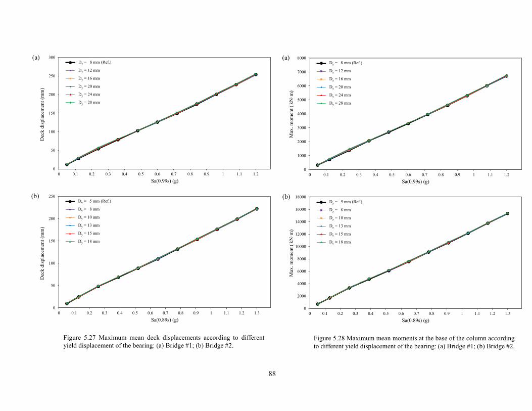
88

0

50

100

150

200

250

300

0 0.1 0.2 0.3 0.4 0.5 0.6 0.7 0.8 0.9 1 1.1 1.2

Dec

k d

isp

lace

men

t (m

m)

Sa(0.99s) (g)

Dy = 8mm (Ref.)

Dy = 12mm

Dy = 16mm

Dy = 20mm

Dy = 24mm

Dy = 28mm

Dy = 8 mm (Ref.)

Dy = 12 mm

Dy = 16 mm

Dy = 20 mm

Dy = 24 mm

Dy = 28 mm

0

50

100

150

200

250

0 0.1 0.2 0.3 0.4 0.5 0.6 0.7 0.8 0.9 1 1.1 1.2 1.3

Dec

k d

isp

lace

men

t (m

m)

Sa(0.89s) (g)

Dy = 5mm (Ref.)

Dy = 8mm

Dy = 10mm

Dy = 13mm

Dy = 15mm

Dy = 18mm

Dy = 5 mm (Ref.)

Dy = 8 mm

Dy = 10 mm

Dy = 13 mm

Dy = 15 mm

Dy = 18 mm

(a)

(b)


yield displacement of the bearing: (a) Bridge #1; (b) Bridge #2.

0

1000

2000

3000

4000

5000

6000

7000

8000

0 0.1 0.2 0.3 0.4 0.5 0.6 0.7 0.8 0.9 1 1.1 1.2

Max

. m

om

ent

(k

N·m

)

Sa(0.99s) (g)

Dy = 8mm (Ref.)

Dy = 12mm

Dy = 16mm

Dy = 20mm

Dy = 24mm

Dy = 28mm

Dy = 8 mm (Ref.)

Dy = 12 mm

Dy = 16 mm

Dy = 20 mm

Dy = 24 mm

Dy = 28 mm

0

2000

4000

6000

8000

10000

12000

14000

16000

18000

0 0.1 0.2 0.3 0.4 0.5 0.6 0.7 0.8 0.9 1 1.1 1.2 1.3

Max

. m

om

ent

(k

N·m

)

Sa(0.89s) (g)

Dy = 5mm (Ref.)

Dy = 8mm

Dy = 10mm

Dy = 13mm

Dy = 15mm

Dy = 18mm

Dy = 5 mm (Ref.)

Dy = 8 mm

Dy = 10 mm

Dy = 13 mm

Dy = 15 mm

Dy = 18 mm

(a)

(b)


to different yield displacement of the bearing: (a) Bridge #1; (b) Bridge #2.

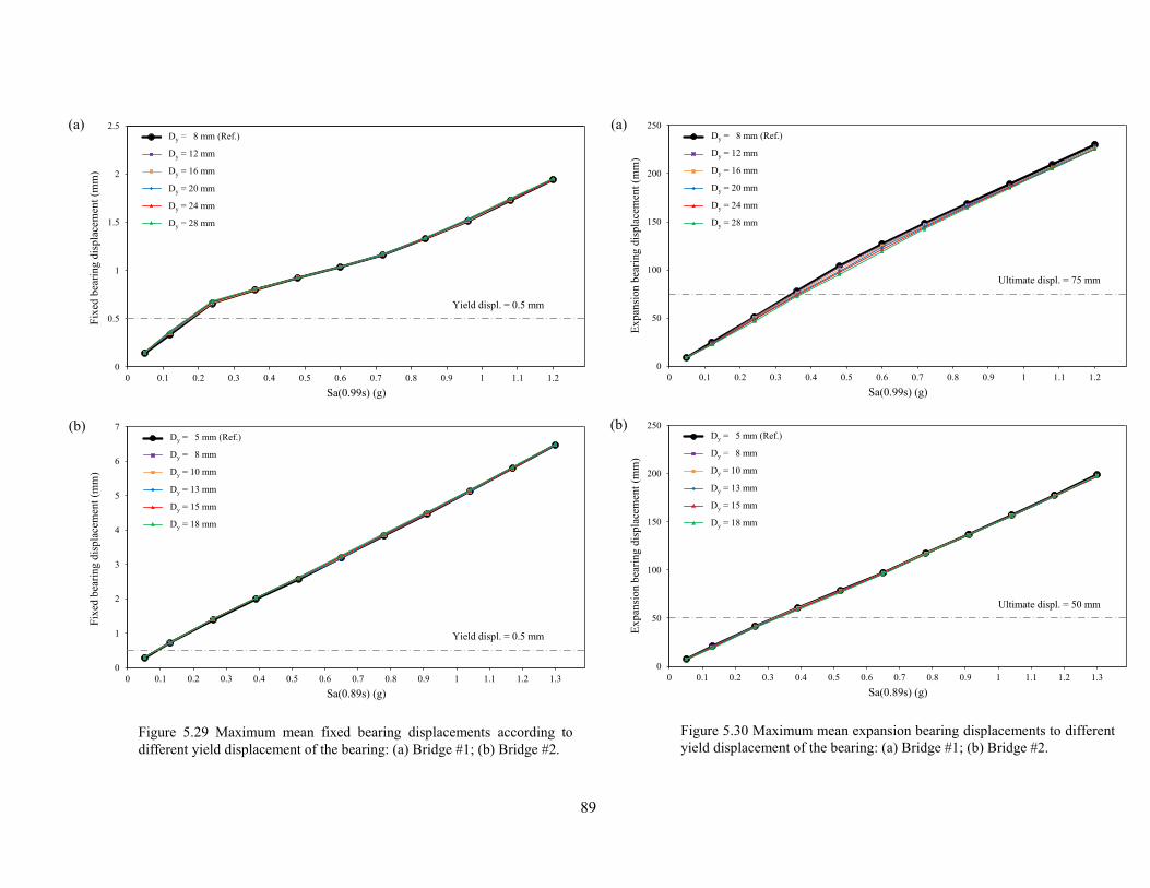
89

0

50

100

150

200

250

0 0.1 0.2 0.3 0.4 0.5 0.6 0.7 0.8 0.9 1 1.1 1.2

Ex

pan

sio

n b

eari

ng d

isp

lace

men

t (m

m)

Sa(0.99s) (g)

Dy = 8mm (Ref.)

Dy = 12mm

Dy = 16mm

Dy = 20mm

Dy = 24mm

Dy = 28mm

Dy = 8 mm (Ref.)

Dy = 12 mm

Dy = 16 mm

Dy = 20 mm

Dy = 24 mm

Dy = 28 mm


0

50

100

150

200

250

0 0.1 0.2 0.3 0.4 0.5 0.6 0.7 0.8 0.9 1 1.1 1.2 1.3

Ex

pan

sio

n b

eari

ng d

isp

lace

men

t (m

m)

Sa(0.89s) (g)

Dy = 5mm (Ref.)

Dy = 8mm

Dy = 10mm

Dy = 13mm

Dy = 15mm

Dy = 18mm

Dy = 5 mm (Ref.)

Dy = 8 mm

Dy = 10 mm

Dy = 13 mm

Dy = 15 mm

Dy = 18 mm


(a)

(b)

Figure 5.30 Maximum mean expansion bearing displacements to different

yield displacement of the bearing: (a) Bridge #1; (b) Bridge #2.

0

0.5

1

1.5

2

2.5

0 0.1 0.2 0.3 0.4 0.5 0.6 0.7 0.8 0.9 1 1.1 1.2

Fix

ed b

eari

ng d

isp

lace

men

t (m

m)

Sa(0.99s) (g)

Dy = 8mm (Ref.)

Dy = 12mm

Dy = 16mm

Dy = 20mm

Dy = 24mm

Dy = 28mm

Dy = 8 mm (Ref.)

Dy = 12 mm

Dy = 16 mm

Dy = 20 mm

Dy = 24 mm

Dy = 28 mm


0

1

2

3

4

5

6

7

0 0.1 0.2 0.3 0.4 0.5 0.6 0.7 0.8 0.9 1 1.1 1.2 1.3

Fix

ed b

eari

ng d

isp

lace

men

t (m

m)

Sa(0.89s) (g)

Dy = 5mm (Ref.)

Dy = 8mm

Dy = 10mm

Dy = 13mm

Dy = 15mm

Dy = 18mm

Dy = 5 mm (Ref.)

Dy = 8 mm

Dy = 10 mm

Dy = 13 mm

Dy = 15 mm

Dy = 18 mm


(a)

(b)


different yield displacement of the bearing: (a) Bridge #1; (b) Bridge #2.

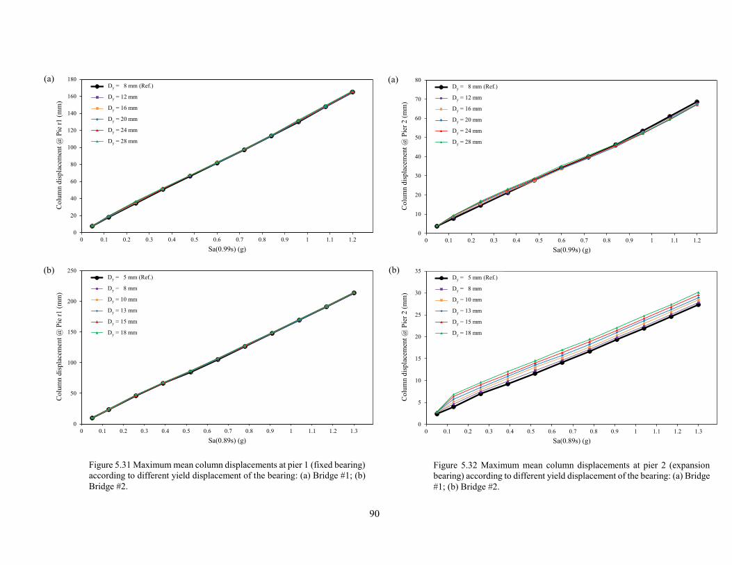
90

0

20

40

60

80

100

120

140

160

180

0 0.1 0.2 0.3 0.4 0.5 0.6 0.7 0.8 0.9 1 1.1 1.2

Co

lum

n d

isp

lace

men

t @

Pie

r1

(m

m)

Sa(0.99s) (g)

Dy = 8mm (Ref.)

Dy = 12mm

Dy = 16mm

Dy = 20mm

Dy = 24mm

Dy = 28mm

Dy = 8 mm (Ref.)

Dy = 12 mm

Dy = 16 mm

Dy = 20 mm

Dy = 24 mm

Dy = 28 mm

0

50

100

150

200

250

0 0.1 0.2 0.3 0.4 0.5 0.6 0.7 0.8 0.9 1 1.1 1.2 1.3

Co

lum

n d

isp

lace

men

t @

Pie

r1

(m

m)

Sa(0.89s) (g)

Dy = 5mm (Ref.)

Dy = 8mm

Dy = 10mm

Dy = 13mm

Dy = 15mm

Dy = 18mm

Dy = 5 mm (Ref.)

Dy = 8 mm

Dy = 10 mm

Dy = 13 mm

Dy = 15 mm

Dy = 18 mm

(a)

(b)


according to different yield displacement of the bearing: (a) Bridge #1; (b)

Bridge #2.

0

10

20

30

40

50

60

70

80

0 0.1 0.2 0.3 0.4 0.5 0.6 0.7 0.8 0.9 1 1.1 1.2

Co

lum

n d

isp

lace

men

t @

Pie

r 2

(m

m)

Sa(0.99s) (g)

Dy = 8mm (Ref.)

Dy = 12mm

Dy = 16mm

Dy = 20mm

Dy = 24mm

Dy = 28mm

Dy = 8 mm (Ref.)

Dy = 12 mm

Dy = 16 mm

Dy = 20 mm

Dy = 24 mm

Dy = 28 mm

0

5

10

15

20

25

30

35

0 0.1 0.2 0.3 0.4 0.5 0.6 0.7 0.8 0.9 1 1.1 1.2 1.3

Co

lum

n d

isp

lace

men

t @

Pie

r 2

(m

m)

Sa(0.89s) (g)

Dy = 5mm (Ref.)

Dy = 8mm

Dy = 10mm

Dy = 13mm

Dy = 15mm

Dy = 18mm

Dy = 5 mm (Ref.)

Dy = 8 mm

Dy = 10 mm

Dy = 13 mm

Dy = 15 mm

Dy = 18 mm

(a)

(b)


bearing) according to different yield displacement of the bearing: (a) Bridge

#1; (b) Bridge #2.

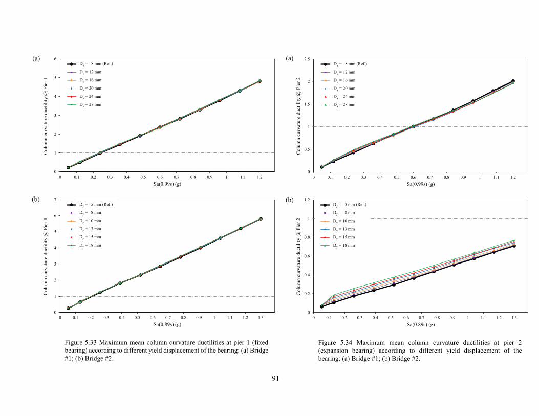
91

0

0.5

1

1.5

2

2.5

0 0.1 0.2 0.3 0.4 0.5 0.6 0.7 0.8 0.9 1 1.1 1.2

Co

lum

n c

urv

atu

re d

uct

ilit

y @

Pie

r 2

Sa(0.99s) (g)

Dy = 8mm (Ref.)

Dy = 12mm

Dy = 16mm

Dy = 20mm

Dy = 24mm

Dy = 28mm

Dy = 8 mm (Ref.)

Dy = 12 mm

Dy = 16 mm

Dy = 20 mm

Dy = 24 mm

Dy = 28 mm

0

0.2

0.4

0.6

0.8

1

1.2

0 0.1 0.2 0.3 0.4 0.5 0.6 0.7 0.8 0.9 1 1.1 1.2 1.3

Co

lum

n c

urv

atu

re d

uct

ilit

y @

Pie

r 2

Sa(0.89s) (g)

Dy = 5mm (Ref.)

Dy = 8mm

Dy = 10mm

Dy = 13mm

Dy = 15mm

Dy = 18mm

Dy = 5 mm (Ref.)

Dy = 8 mm

Dy = 10 mm

Dy = 13 mm

Dy = 15 mm

Dy = 18 mm

(a)

(b)


(expansion bearing) according to different yield displacement of the

bearing: (a) Bridge #1; (b) Bridge #2.

0

1

2

3

4

5

6

0 0.1 0.2 0.3 0.4 0.5 0.6 0.7 0.8 0.9 1 1.1 1.2

Co

lum

n c

urv

atu

re d

uct

ilit

y @

Pie

r 1

Sa(0.99s) (g)

Dy = 8mm (Ref.)

Dy = 12mm

Dy = 16mm

Dy = 20mm

Dy = 24mm

Dy = 28mm

Dy = 8 mm (Ref.)

Dy = 12 mm

Dy = 16 mm

Dy = 20 mm

Dy = 24 mm

Dy = 28 mm

0

1

2

3

4

5

6

7

0 0.1 0.2 0.3 0.4 0.5 0.6 0.7 0.8 0.9 1 1.1 1.2 1.3

Co

lum

n c

urv

atu

re d

uct

ilit

y @

Pie

r 1

Sa(0.89s) (g)

Dy = 5mm (Ref.)

Dy = 8mm

Dy = 10mm

Dy = 13mm

Dy = 15mm

Dy = 18mm

Dy = 5 mm (Ref.)

Dy = 8 mm

Dy = 10 mm

Dy = 13 mm

Dy = 15 mm

Dy = 18 mm

(a)

(b)


bearing) according to different yield displacement of the bearing: (a) Bridge

#1; (b) Bridge #2.

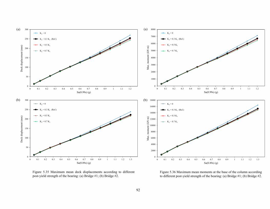
92

0

1000

2000

3000

4000

5000

6000

7000

8000

0 0.1 0.2 0.3 0.4 0.5 0.6 0.7 0.8 0.9 1 1.1 1.2

Max

. m

om

ent

(k

N·m

)

Sa(0.99s) (g)

K2 = 0

K2 = 0.3K1 (Ref.)

K2 = 0.5K1

K2 = 0.7K1

K2 = 0

K2 = 0.3 K1 (Ref.)

K2 = 0.5 K1

K2 = 0.7 K1

0

2000

4000

6000

8000

10000

12000

14000

16000

18000

0 0.1 0.2 0.3 0.4 0.5 0.6 0.7 0.8 0.9 1 1.1 1.2 1.3

Max

. m

om

ent

(k

N·m

)

Sa(0.89s) (g)

K2 = 0

K2 = 0.3K1 (Ref.)

K2 = 0.5K1

K2 = 0.7K1

K2 = 0

K2 = 0.3 K1 (Ref.)

K2 = 0.5 K1

K2 = 0.7 K1

(a)

(b)


to different post-yield strength of the bearing: (a) Bridge #1; (b) Bridge #2.

0

50

100

150

200

250

300

0 0.1 0.2 0.3 0.4 0.5 0.6 0.7 0.8 0.9 1 1.1 1.2

Dec

k d

isp

lace

men

t (m

m)

Sa(0.99s) (g)

K2 = 0

K2 = 0.3K1 (Ref.)

K2 = 0.5K1

K2 = 0.7K1

K2 = 0

K2 = 0.3 K1 (Ref.)

K2 = 0.5 K1

K2 = 0.7 K1

0

50

100

150

200

250

300

0 0.1 0.2 0.3 0.4 0.5 0.6 0.7 0.8 0.9 1 1.1 1.2 1.3

Dec

k d

isp

lace

men

t (m

m)

Sa(0.89s) (g)

K2 = 0

K2 = 0.3K1 (Ref.)

K2 = 0.5K1

K2 = 0.7K1

K2 = 0

K2 = 0.3 K1 (Ref.)

K2 = 0.5 K1

K2 = 0.7 K1

(a)

(b)


post-yield strength of the bearing: (a) Bridge #1; (b) Bridge #2.

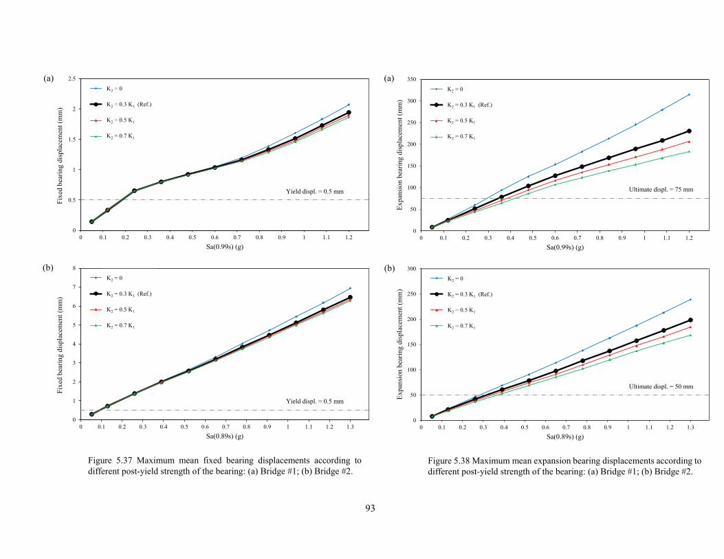
93

0

0.5

1

1.5

2

2.5

0 0.1 0.2 0.3 0.4 0.5 0.6 0.7 0.8 0.9 1 1.1 1.2

Fix

ed b

eari

ng d

isp

lace

men

t (m

m)

Sa(0.99s) (g)

K2 = 0

K2 = 0.3K1 (Ref.)

K2 = 0.5K1

K2 = 0.7K1

K2 = 0

K2 = 0.3 K1 (Ref.)

K2 = 0.5 K1

K2 = 0.7 K1


0

1

2

3

4

5

6

7

8

0 0.1 0.2 0.3 0.4 0.5 0.6 0.7 0.8 0.9 1 1.1 1.2 1.3

Fix

ed b

eari

ng d

isp

lace

men

t (m

m)

Sa(0.89s) (g)

K2 = 0

K2 = 0.3K1 (Ref.)

K2 = 0.5K1

K2 = 0.7K1

K2 = 0

K2 = 0.3 K1 (Ref.)

K2 = 0.5 K1

K2 = 0.7 K1


(a)

(b)


different post-yield strength of the bearing: (a) Bridge #1; (b) Bridge #2.

0

50

100

150

200

250

300

350

0 0.1 0.2 0.3 0.4 0.5 0.6 0.7 0.8 0.9 1 1.1 1.2

Ex

pan

sio

n b

eari

ng d

isp

lace

men

t (m

m)

Sa(0.99s) (g)

K2 = 0

K2 = 0.3K1 (Ref.)

K2 = 0.5K1

K2 = 0.7K1

K2 = 0

K2 = 0.3 K1 (Ref.)

K2 = 0.5 K1

K2 = 0.7 K1


0

50

100

150

200

250

300

0 0.1 0.2 0.3 0.4 0.5 0.6 0.7 0.8 0.9 1 1.1 1.2 1.3

Ex

pan

sio

n b

eari

ng d

isp

lace

men

t (m

m)

Sa(0.89s) (g)

K2 = 0

K2 = 0.3K1 (Ref.)

K2 = 0.5K1

K2 = 0.7K1

K2 = 0

K2 = 0.3 K1 (Ref.)

K2 = 0.5 K1

K2 = 0.7 K1


(a)

(b)


different post-yield strength of the bearing: (a) Bridge #1; (b) Bridge #2.

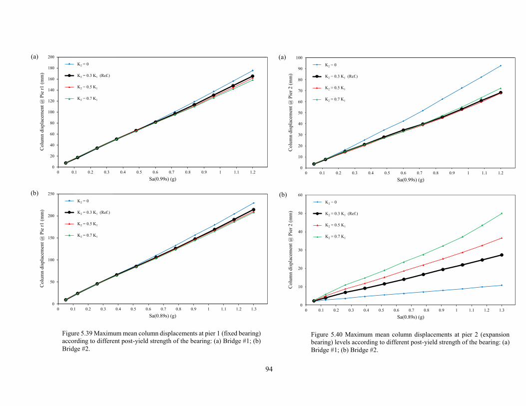
94

0

20

40

60

80

100

120

140

160

180

200

0 0.1 0.2 0.3 0.4 0.5 0.6 0.7 0.8 0.9 1 1.1 1.2

Co

lum

n d

isp

lace

men

t @

Pie

r1

(m

m)

Sa(0.99s) (g)

K2 = 0

K2 = 0.3K1 (Ref.)

K2 = 0.5K1

K2 = 0.7K1

K2 = 0

K2 = 0.3 K1 (Ref.)

K2 = 0.5 K1

K2 = 0.7 K1

0

50

100

150

200

250

0 0.1 0.2 0.3 0.4 0.5 0.6 0.7 0.8 0.9 1 1.1 1.2 1.3

Co

lum

n d

isp

lace

men

t @

Pie

r1

(m

m)

Sa(0.89s) (g)

K2 = 0

K2 = 0.3K1 (Ref.)

K2 = 0.5K1

K2 = 0.7K1

K2 = 0

K2 = 0.3 K1 (Ref.)

K2 = 0.5 K1

K2 = 0.7 K1

(a)

(b)


according to different post-yield strength of the bearing: (a) Bridge #1; (b)

Bridge #2.

0

10

20

30

40

50

60

70

80

90

100

0 0.1 0.2 0.3 0.4 0.5 0.6 0.7 0.8 0.9 1 1.1 1.2

Co

lum

n d

isp

lace

men

t @

Pie

r 2

(m

m)

Sa(0.99s) (g)

K2 = 0

K2 = 0.3K1 (Ref.)

K2 = 0.5K1

K2 = 0.7K1

K2 = 0

K2 = 0.3 K1 (Ref.)

K2 = 0.5 K1

K2 = 0.7 K1

0

10

20

30

40

50

60

0 0.1 0.2 0.3 0.4 0.5 0.6 0.7 0.8 0.9 1 1.1 1.2 1.3

Co

lum

n d

isp

lace

men

t @

Pie

r 2

(m

m)

Sa(0.89s) (g)

K2 = 0

K2 = 0.3K1 (Ref.)

K2 = 0.5K1

K2 = 0.7K1

K2 = 0

K2 = 0.3 K1 (Ref.)

K2 = 0.5 K1

K2 = 0.7 K1

(a)

(b)


bearing) levels according to different post-yield strength of the bearing: (a)


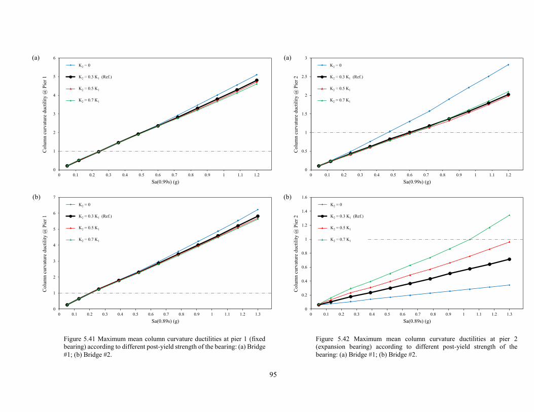
95

0

1

2

3

4

5

6

0 0.1 0.2 0.3 0.4 0.5 0.6 0.7 0.8 0.9 1 1.1 1.2

Co

lum

n c

urv

atu

re d

uct

ilit

y @

Pie

r 1

Sa(0.99s) (g)

K2 = 0

K2 = 0.3K1 (Ref.)

K2 = 0.5K1

K2 = 0.7K1

K2 = 0

K2 = 0.3 K1 (Ref.)

K2 = 0.5 K1

K2 = 0.7 K1

0

1

2

3

4

5

6

7

0 0.1 0.2 0.3 0.4 0.5 0.6 0.7 0.8 0.9 1 1.1 1.2 1.3

Co

lum

n c

urv

atu

re d

uct

ilit

y @

Pie

r 1

Sa(0.89s) (g)

K2 = 0

K2 = 0.3K1 (Ref.)

K2 = 0.5K1

K2 = 0.7K1

K2 = 0

K2 = 0.3 K1 (Ref.)

K2 = 0.5 K1

K2 = 0.7 K1

(a)

(b)


bearing) according to different post-yield strength of the bearing: (a) Bridge

#1; (b) Bridge #2.

0

0.5

1

1.5

2

2.5

3

0 0.1 0.2 0.3 0.4 0.5 0.6 0.7 0.8 0.9 1 1.1 1.2

Co

lum

n c

urv

atu

re d

uct

ilit

y @

Pie

r 2

Sa(0.99s) (g)

K2 = 0

K2 = 0.3K1 (Ref.)

K2 = 0.5K1

K2 = 0.7K1

K2 = 0

K2 = 0.3 K1 (Ref.)

K2 = 0.5 K1

K2 = 0.7 K1

0

0.2

0.4

0.6

0.8

1

1.2

1.4

1.6

0 0.1 0.2 0.3 0.4 0.5 0.6 0.7 0.8 0.9 1 1.1 1.2 1.3

Co

lum

n c

urv

atu

re d

uct

ilit

y @

Pie

r 2

Sa(0.89s) (g)

K2 = 0

K2 = 0.3K1 (Ref.)

K2 = 0.5K1

K2 = 0.7K1

K2 = 0

K2 = 0.3 K1 (Ref.)

K2 = 0.5 K1

K2 = 0.7 K1

(a)

(b)


(expansion bearing) according to different post-yield strength of the

bearing: (a) Bridge #1; (b) Bridge #2.

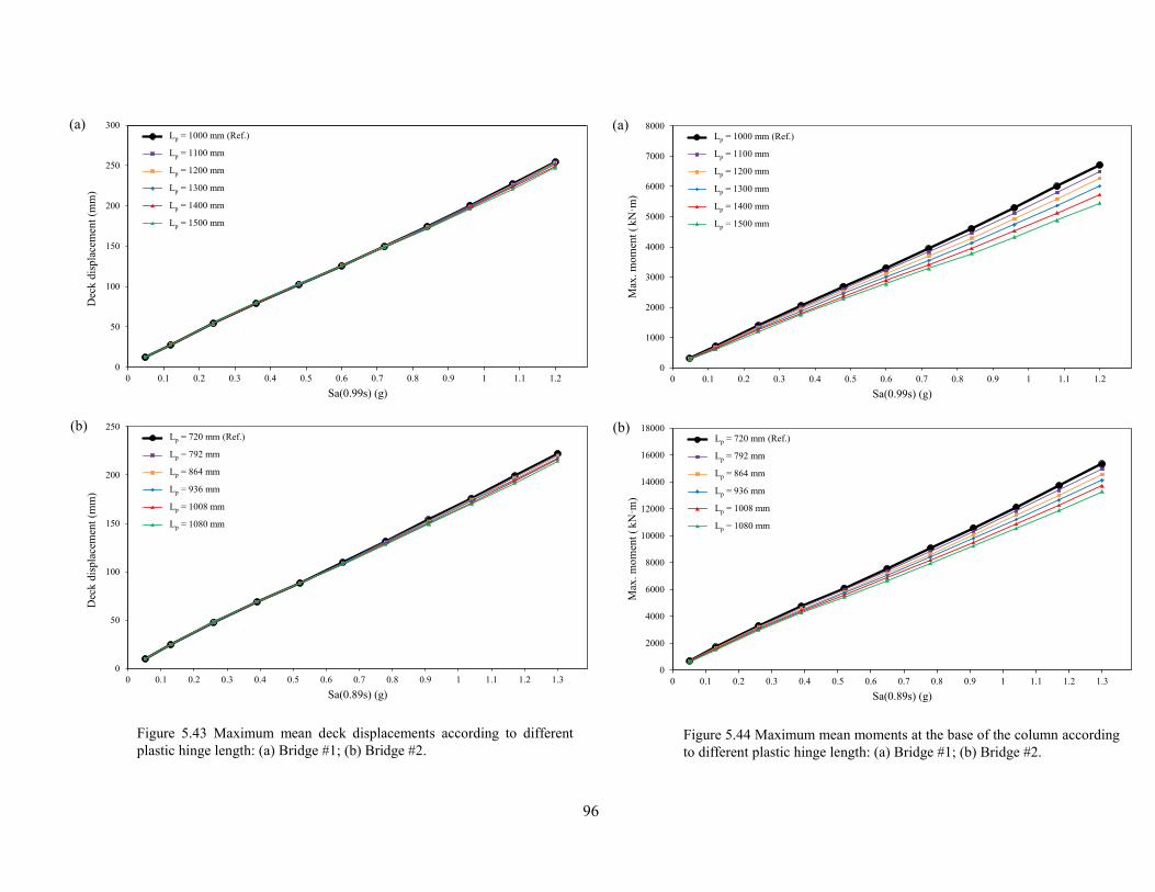
96

0

1000

2000

3000

4000

5000

6000

7000

8000

0 0.1 0.2 0.3 0.4 0.5 0.6 0.7 0.8 0.9 1 1.1 1.2

Max

. m

om

ent

(k

N·m

)

Sa(0.99s) (g)

Lp = 1000 mm (Ref.)

Lp = 1100 mm

Lp = 1200 mm

Lp = 1300 mm

Lp = 1400 mm

Lp = 1500 mm

Lp = 1000 mm (Ref.)

Lp = 1100 mm

Lp = 1200 mm

Lp = 1300 mm

Lp = 1400 mm

Lp = 1500 mm

0

2000

4000

6000

8000

10000

12000

14000

16000

18000

0 0.1 0.2 0.3 0.4 0.5 0.6 0.7 0.8 0.9 1 1.1 1.2 1.3

Max

. m

om

ent

(k

N·m

)

Sa(0.89s) (g)

Lp = 720mm (Ref.)

Lp = 792mm

Lp = 864mm

Lp = 936mm

Lp = 1008mm

Lp = 10800mm

Lp = 720 mm (Ref.)

Lp = 792 mm

Lp = 864 mm

Lp = 936 mm

Lp = 1008 mm

Lp = 1080 mm

(a)

(b)


to different plastic hinge length: (a) Bridge #1; (b) Bridge #2.

0

50

100

150

200

250

300

0 0.1 0.2 0.3 0.4 0.5 0.6 0.7 0.8 0.9 1 1.1 1.2

Dec

k d

isp

lace

men

t (m

m)

Sa(0.99s) (g)

Lp = 1000 mm (Ref.)

Lp = 1100 mm

Lp = 1200 mm

Lp = 1300 mm

Lp = 1400 mm

Lp = 1500 mm

Lp = 1000 mm (Ref.)

Lp = 1100 mm

Lp = 1200 mm

Lp = 1300 mm

Lp = 1400 mm

Lp = 1500 mm

0

50

100

150

200

250

0 0.1 0.2 0.3 0.4 0.5 0.6 0.7 0.8 0.9 1 1.1 1.2 1.3

Dec

k d

isp

lace

men

t (m

m)

Sa(0.89s) (g)

Lp = 720mm (Ref.)

Lp = 792mm

Lp = 864mm

Lp = 1008mm

Lp = 1008mm

Lp = 10800mm

Lp = 720 mm (Ref.)

Lp = 792 mm

Lp = 864 mm

Lp = 936 mm

Lp = 1008 mm

Lp = 1080 mm

(a)

(b)


plastic hinge length: (a) Bridge #1; (b) Bridge #2.

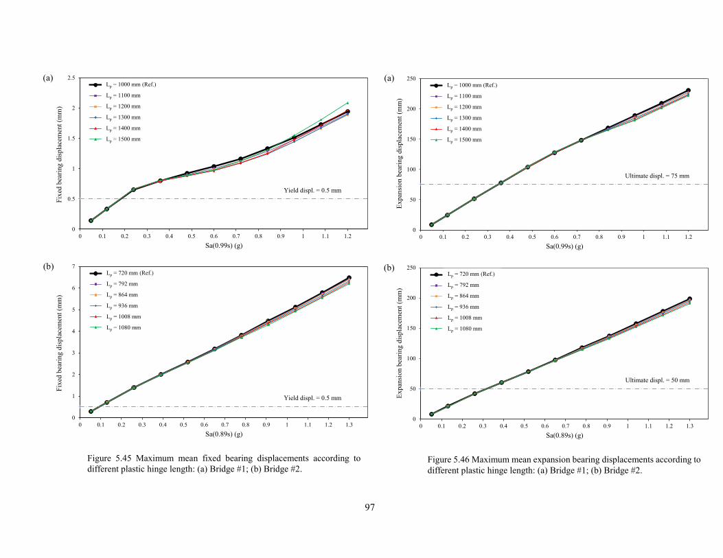
97

0

50

100

150

200

250

0 0.1 0.2 0.3 0.4 0.5 0.6 0.7 0.8 0.9 1 1.1 1.2

Ex

pan

sio

n b

eari

ng d

isp

lace

men

t (m

m)

Sa(0.99s) (g)

Lp = 1000 mm (Ref.)

Lp = 1100 mm

Lp = 1200 mm

Lp = 1300 mm

Lp = 1400 mm

Lp = 1500 mm

Lp = 1000 mm (Ref.)

Lp = 1100 mm

Lp = 1200 mm

Lp = 1300 mm

Lp = 1400 mm

Lp = 1500 mm


0

50

100

150

200

250

0 0.1 0.2 0.3 0.4 0.5 0.6 0.7 0.8 0.9 1 1.1 1.2 1.3

Ex

pan

sio

n b

eari

ng d

isp

lace

men

t (m

m)

Sa(0.89s) (g)

Lp = 720mm (Ref.)

Lp = 792mm

Lp = 864mm

Lp = 936mm

Lp = 1008mm

Lp = 10800mm

Lp = 720 mm (Ref.)

Lp = 792 mm

Lp = 864 mm

Lp = 936 mm

Lp = 1008 mm

Lp = 1080 mm


(a)

(b)


different plastic hinge length: (a) Bridge #1; (b) Bridge #2.

0

0.5

1

1.5

2

2.5

0 0.1 0.2 0.3 0.4 0.5 0.6 0.7 0.8 0.9 1 1.1 1.2

Fix

ed b

eari

ng d

isp

lace

men

t (m

m)

Sa(0.99s) (g)

Lp = 1000 mm (Ref.)

Lp = 1100 mm

Lp = 1200 mm

Lp = 1300 mm

Lp = 1400 mm

Lp = 1500 mm

Lp = 1000 mm (Ref.)

Lp = 1100 mm

Lp = 1200 mm

Lp = 1300 mm

Lp = 1400 mm

Lp = 1500 mm


0

1

2

3

4

5

6

7

0 0.1 0.2 0.3 0.4 0.5 0.6 0.7 0.8 0.9 1 1.1 1.2 1.3

Fix

ed b

eari

ng d

isp

lace

men

t (m

m)

Sa(0.89s) (g)

Lp = 720mm (Ref.)

Lp = 792mm

Lp = 864mm

Lp = 936mm

Lp = 1008mm

Lp = 10800mm

Lp = 720 mm (Ref.)

Lp = 792 mm

Lp = 864 mm

Lp = 936 mm

Lp = 1008 mm

Lp = 1080 mm


(a)

(b)


different plastic hinge length: (a) Bridge #1; (b) Bridge #2.

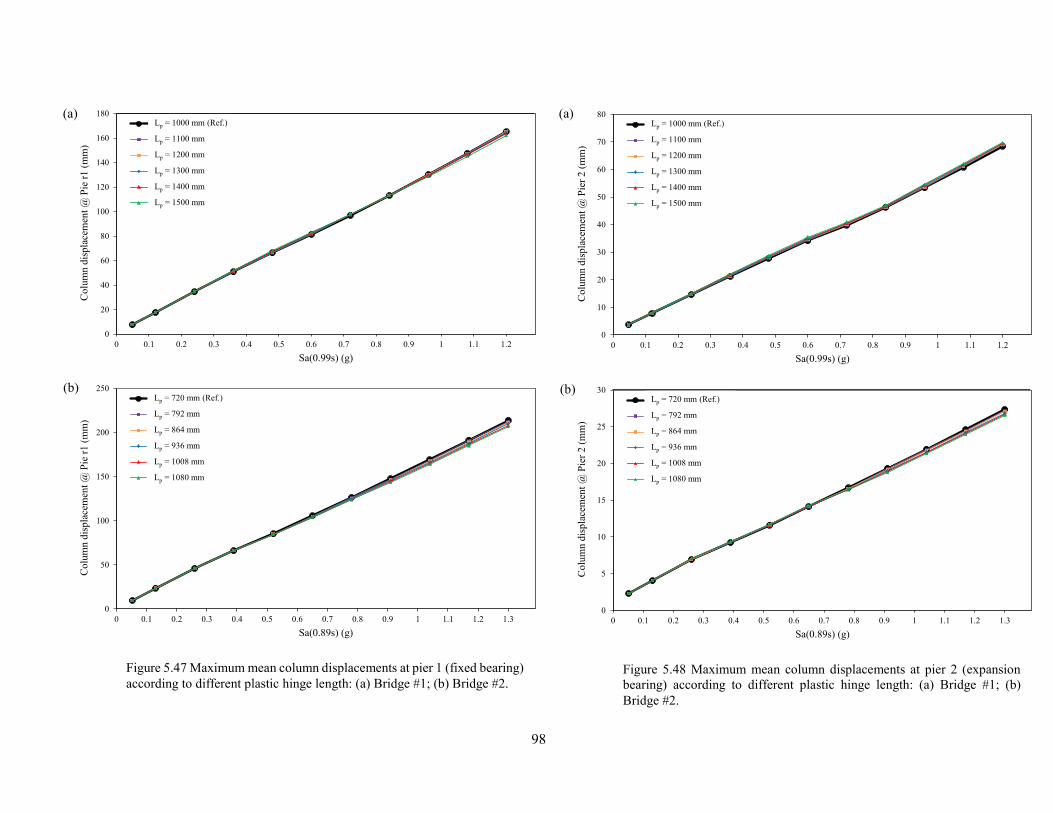
98

0

20

40

60

80

100

120

140

160

180

0 0.1 0.2 0.3 0.4 0.5 0.6 0.7 0.8 0.9 1 1.1 1.2

Co

lum

n d

isp

lace

men

t @

Pie

r1

(m

m)

Sa(0.99s) (g)

Lp = 1000 mm (Ref.)

Lp = 1100 mm

Lp = 1200 mm

Lp = 1300 mm

Lp = 1400 mm

Lp = 1500 mm

Lp = 1000 mm (Ref.)

Lp = 1100 mm

Lp = 1200 mm

Lp = 1300 mm

Lp = 1400 mm

Lp = 1500 mm

0

50

100

150

200

250

0 0.1 0.2 0.3 0.4 0.5 0.6 0.7 0.8 0.9 1 1.1 1.2 1.3

Co

lum

n d

isp

lace

men

t @

Pie

r1

(m

m)

Sa(0.89s) (g)

Lp = 720mm (Ref.)

Lp = 792mm

Lp = 864mm

Lp = 936mm

Lp = 1008mm

Lp = 10800mm

Lp = 720 mm (Ref.)

Lp = 792 mm

Lp = 864 mm

Lp = 936 mm

Lp = 1008 mm

Lp = 1080 mm

(a)

(b)


according to different plastic hinge length: (a) Bridge #1; (b) Bridge #2.

0

10

20

30

40

50

60

70

80

0 0.1 0.2 0.3 0.4 0.5 0.6 0.7 0.8 0.9 1 1.1 1.2

Co

lum

n d

isp

lace

men

t @

Pie

r 2

(m

m)

Sa(0.99s) (g)

Lp = 1000 mm (Ref.)

Lp = 1100 mm

Lp = 1200 mm

Lp = 1300 mm

Lp = 1400 mm

Lp = 1500 mm

Lp = 1000 mm (Ref.)

Lp = 1100 mm

Lp = 1200 mm

Lp = 1300 mm

Lp = 1400 mm

Lp = 1500 mm

0

5

10

15

20

25

30

0 0.1 0.2 0.3 0.4 0.5 0.6 0.7 0.8 0.9 1 1.1 1.2 1.3

Co

lum

n d

isp

lace

men

t @

Pie

r 2

(m

m)

Sa(0.89s) (g)

Lp = 720mm (Ref.)

Lp = 792mm

Lp = 864mm

Lp = 936mm

Lp = 1008mm

Lp = 10800mm

Lp = 720 mm (Ref.)

Lp = 792 mm

Lp = 864 mm

Lp = 936 mm

Lp = 1008 mm

Lp = 1080 mm

(a)

(b)


bearing) according to different plastic hinge length: (a) Bridge #1; (b)

Bridge #2.

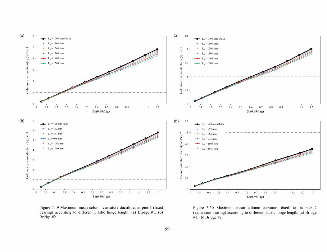
99

0

0.5

1

1.5

2

2.5

0 0.1 0.2 0.3 0.4 0.5 0.6 0.7 0.8 0.9 1 1.1 1.2

Co

lum

n c

urv

atu

re d

uct

ilit

y @

Pie

r 2

Sa(0.99s) (g)

Lp = 1000 mm (Ref.)

Lp = 1100 mm

Lp = 1200 mm

Lp = 1300 mm

Lp = 1400 mm

Lp = 1500 mm

Lp = 1000 mm (Ref.)

Lp = 1100 mm

Lp = 1200 mm

Lp = 1300 mm

Lp = 1400 mm

Lp = 1500 mm

0

0.2

0.4

0.6

0.8

1

1.2

0 0.1 0.2 0.3 0.4 0.5 0.6 0.7 0.8 0.9 1 1.1 1.2 1.3

Co

lum

n c

urv

atu

re d

uct

ilit

y @

Pie

r 2

Sa(0.89s) (g)

Lp = 720mm (Ref.)

Lp = 792mm

Lp = 864mm

Lp = 936mm

Lp = 1008mm

Lp = 10800mm

Lp = 720 mm (Ref.)

Lp = 792 mm

Lp = 864 mm

Lp = 936 mm

Lp = 1008 mm

Lp = 1080 mm

(a)

(b)


(expansion bearing) according to different plastic hinge length: (a) Bridge

#1; (b) Bridge #2.

0

1

2

3

4

5

6

0 0.1 0.2 0.3 0.4 0.5 0.6 0.7 0.8 0.9 1 1.1 1.2

Co

lum

n c

urv

atu

re d

uct

ilit

y @

Pie

r 1

Sa(0.99s) (g)

Lp = 1000 mm (Ref.)

Lp = 1100 mm

Lp = 1200 mm

Lp = 1300 mm

Lp = 1400 mm

Lp = 1500 mm

Lp = 1000 mm (Ref.)

Lp = 1100 mm

Lp = 1200 mm

Lp = 1300 mm

Lp = 1400 mm

Lp = 1500 mm

0

1

2

3

4

5

6

7

0 0.1 0.2 0.3 0.4 0.5 0.6 0.7 0.8 0.9 1 1.1 1.2 1.3

Co

lum

n c

urv

atu

re d

uct

ilit

y @

Pie

r 1

Sa(0.89s) (g)

Lp = 720mm (Ref.)

Lp = 792mm

Lp = 864mm

Lp = 936mm

Lp = 1008mm

Lp = 10800mm

Lp = 720 mm (Ref.)

Lp = 792 mm

Lp = 864 mm

Lp = 936 mm

Lp = 1008 mm

Lp = 1080 mm

(a)

(b)


bearing) according to different plastic hinge length: (a) Bridge #1; (b)

Bridge #2.

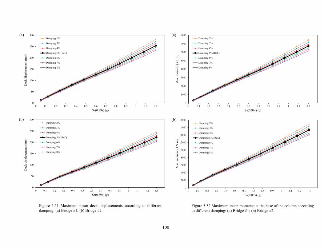
100

0

50

100

150

200

250

300

0 0.1 0.2 0.3 0.4 0.5 0.6 0.7 0.8 0.9 1 1.1 1.2

Dec

k d

isp

lace

men

t (m

m)

Sa(0.99s) (g)

Damping 2%

Damping 3%

Damping 4%

Damping 5% (Ref.)

Damping 6%

Damping 7%

Damping 8%

0

50

100

150

200

250

300

0 0.1 0.2 0.3 0.4 0.5 0.6 0.7 0.8 0.9 1 1.1 1.2 1.3

Dec

k d

isp

lace

men

t (m

m)

Sa(0.89s) (g)

Damping 2%

Damping 3%

Damping 4%

Damping 5% (Ref.)

Damping 6%

Damping 7%

Damping 8%

(a)

(b)


damping: (a) Bridge #1; (b) Bridge #2.

0

1000

2000

3000

4000

5000

6000

7000

8000

0 0.1 0.2 0.3 0.4 0.5 0.6 0.7 0.8 0.9 1 1.1 1.2

Max

. m

om

ent

(k

N·m

)

Sa(0.99s) (g)

Damping 2%

Damping 3%

Damping 4%

Damping 5% (Ref.)

Damping 6%

Damping 7%

Damping 8%

0

2000

4000

6000

8000

10000

12000

14000

16000

18000

0 0.1 0.2 0.3 0.4 0.5 0.6 0.7 0.8 0.9 1 1.1 1.2 1.3

Max

. m

om

ent

(k

N·m

)

Sa(0.89s) (g)

Damping 2%

Damping 3%

Damping 4%

Damping 5% (Ref.)

Damping 6%

Damping 7%

Damping 8%

(a)

(b)


to different damping: (a) Bridge #1; (b) Bridge #2.

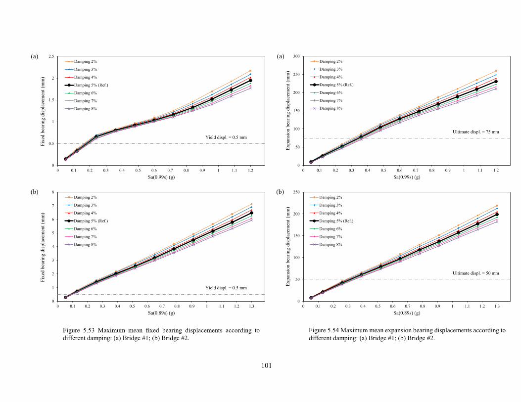
101

0

1

2

3

4

5

6

7

8

0 0.1 0.2 0.3 0.4 0.5 0.6 0.7 0.8 0.9 1 1.1 1.2 1.3

Fix

ed b

eari

ng d

isp

lace

men

t (m

m)

Sa(0.89s) (g)

Damping 2%

Damping 3%

Damping 4%

Damping 5% (Ref.)

Damping 6%

Damping 7%

Damping 8%


0

0.5

1

1.5

2

2.5

0 0.1 0.2 0.3 0.4 0.5 0.6 0.7 0.8 0.9 1 1.1 1.2

Fix

ed b

eari

ng d

isp

lace

men

t (m

m)

Sa(0.99s) (g)

Damping 2%

Damping 3%

Damping 4%

Damping 5% (Ref.)

Damping 6%

Damping 7%

Damping 8%


(a)

(b)


different damping: (a) Bridge #1; (b) Bridge #2.

0

50

100

150

200

250

300

0 0.1 0.2 0.3 0.4 0.5 0.6 0.7 0.8 0.9 1 1.1 1.2

Ex

pan

sio

n b

eari

ng d

isp

lace

men

t (m

m)

Sa(0.99s) (g)

Damping 2%

Damping 3%

Damping 4%

Damping 5% (Ref.)

Damping 6%

Damping 7%

Damping 8%


0

50

100

150

200

250

0 0.1 0.2 0.3 0.4 0.5 0.6 0.7 0.8 0.9 1 1.1 1.2 1.3

Ex

pan

sio

n b

eari

ng d

isp

lace

men

t (m

m)

Sa(0.89s) (g)

Damping 2%

Damping 3%

Damping 4%

Damping 5% (Ref.)

Damping 6%

Damping 7%

Damping 8%


(a)

(b)


different damping: (a) Bridge #1; (b) Bridge #2.

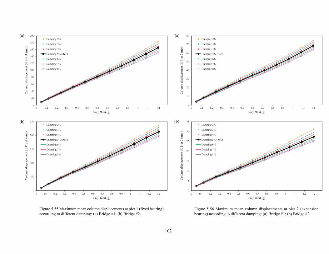
102

0

20

40

60

80

100

120

140

160

180

200

0 0.1 0.2 0.3 0.4 0.5 0.6 0.7 0.8 0.9 1 1.1 1.2

Co

lum

n d

isp

lace

men

t @

Pie

r1

(m

m)

Sa(0.99s) (g)

Damping 2%

Damping 3%

Damping 4%

Damping 5% (Ref.)

Damping 6%

Damping 7%

Damping 8%

0

50

100

150

200

250

0 0.1 0.2 0.3 0.4 0.5 0.6 0.7 0.8 0.9 1 1.1 1.2 1.3

Co

lum

n d

isp

lace

men

t @

Pie

r1

(m

m)

Sa(0.89s) (g)

Damping 2%

Damping 3%

Damping 4%

Damping 5% (Ref.)

Damping 6%

Damping 7%

Damping 8%

(a)

(b)


according to different damping: (a) Bridge #1; (b) Bridge #2.

0

10

20

30

40

50

60

70

80

0 0.1 0.2 0.3 0.4 0.5 0.6 0.7 0.8 0.9 1 1.1 1.2

Co

lum

n d

isp

lace

men

t @

Pie

r 2

(m

m)

Sa(0.99s) (g)

Damping 2%

Damping 3%

Damping 4%

Damping 5% (Ref.)

Damping 6%

Damping 7%

Damping 8%

0

5

10

15

20

25

30

35

0 0.1 0.2 0.3 0.4 0.5 0.6 0.7 0.8 0.9 1 1.1 1.2 1.3

Co

lum

n d

isp

lace

men

t @

Pie

r 2

(m

m)

Sa(0.89s) (g)

Damping 2%

Damping 3%

Damping 4%

Damping 5% (Ref.)

Damping 6%

Damping 7%

Damping 8%

(a)

(b)


bearing) according to different damping: (a) Bridge #1; (b) Bridge #2.

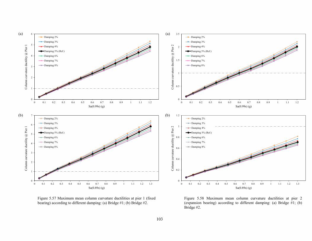
103

0

1

2

3

4

5

6

0 0.1 0.2 0.3 0.4 0.5 0.6 0.7 0.8 0.9 1 1.1 1.2

Co

lum

n c

urv

atu

re d

uct

ilit

y @

Pie

r 1

Sa(0.99s) (g)

Damping 2%

Damping 3%

Damping 4%

Damping 5% (Ref.)

Damping 6%

Damping 7%

Damping 8%

0

1

2

3

4

5

6

7

0 0.1 0.2 0.3 0.4 0.5 0.6 0.7 0.8 0.9 1 1.1 1.2 1.3

Co

lum

n c

urv

atu

re d

uct

ilit

y @

Pie

r 1

Sa(0.89s) (g)

Damping 2%

Damping 3%

Damping 4%

Damping 5% (Ref.)

Damping 6%

Damping 7%

Damping 8%

(a)

(b)


bearing) according to different damping: (a) Bridge #1; (b) Bridge #2.

0

0.5

1

1.5

2

2.5

0 0.1 0.2 0.3 0.4 0.5 0.6 0.7 0.8 0.9 1 1.1 1.2

Co

lum

n c

urv

atu

re d

uct

ilit

y @

Pie

r 2

Sa(0.99s) (g)

Damping 2%

Damping 3%

Damping 4%

Damping 5% (Ref.)

Damping 6%

Damping 7%

Damping 8%

0

0.2

0.4

0.6

0.8

1

1.2

0 0.1 0.2 0.3 0.4 0.5 0.6 0.7 0.8 0.9 1 1.1 1.2 1.3

Co

lum

n c

urv

atu

re d

uct

ilit

y @

Pie

r 2

Sa(0.89s) (g)

Damping 2%

Damping 3%

Damping 4%

Damping 5% (Ref.)

Damping 6%

Damping 7%

Damping 8%

(a)

(b)


(expansion bearing) according to different damping: (a) Bridge #1; (b)

Bridge #2.

104

Chapter 6

Discussion and Conclusions

6.1 Discussion

It has been reported that significant earthquakes could cause severe damage to bridges,

such as, the 1995 M7.2 Kobe earthquake, the 1989 M7.8 Loma Prieta earthquake, etc. In

addition, moderate earthquakes can also cause damage or even collapse of bridges or bridge

components. One typical example is the M5.0 Val-des-Bois earthquake occurred about 60 km

from Ottawa on June 23, 2010. A bridge embankment which close to the epicentre collapsed

and three landslides were triggered in unstable soil deposits during this event.

The lessons from the past earthquakes lead to sustainable research on the seismic

evaluation of bridges. Two methods are typically used for the study: one is deterministic

approach which is applied to a specific bridge, the other is probabilistic approach which is used

for the investigation of bridge portfolios. It has been noticed that earthquakes occurred quite

often in the last several years. For example, 2010 M7.0 Haiti Earthquake, 2010 M8.8 Chile

Earthquake, 2011 M9.0 Japan Earthquake (Tohoku), 2011 M7.2 Alaska Earthquake, and 2011

M7.6 New Zealand Earthquake. Given this, there is an urgent need to conduct seismic risk

analysis on bridges on a large scale (i.e., a specific region or a city) in addition to a specific

bridge due to the importance of bridges in a transportation system. It is necessary to mention

herein that seismic risk assessment of bridge portfolios is needed in order to estimate the

economic losses of the transportation system in a specific area due to potential future

105

earthquakes. The estimation will, in turn, help the government make an emergence plan should

an earthquake happen. However, there is a big challenge for the study because the

configuration of each bridge is unique in terms of the structural system (i.e., simply supported

or continuous), type of the superstructure (i.e., slab-girder type, solid slab deck, single-cell box

girder, multi-cell box girder, etc.), type of the foundation (i.e., shallow foundation, or deep

foundation), number of spans, span length, height of the column, etc. Given this, the

deterministic approach cannot be used for such study since it is not practical to conduct analysis

on each bridge if one wants to investigate the seismic vulnerability of bridges in a large area.

In another word, the probabilistic approach should be considered for the seismic evaluation of

a large population of bridges. In order to use the probabilistic method to assess the seismic

vulnerability of bridge portfolios in a specific zone, types of generic bridges shall be developed

first, which based on the statistics analysis of the current bridge blocks in the zone with

considered of the continuity of the structural system, number of spans, span length, type of the

superstructure, type of the substructure. The features of each bridge within each group, e.g.,

the total length and width of the bridge, material properties (concrete strength and the yield

strength of the steel bar), column height, weight of the superstructure, gap width, property of

bearing including thickness of the bearing and stiffness of bearing and other uncertainties in

the modeling are taken into account by using Monte-Carlo simulation. Since the structural

engineers are not familiar with the Monte-Carlo method, this approach has not been used in

practical applications, i.e., it is mainly used by researchers. In addition, uncertainties of the

modeling parameters should also be considered in the seismic evaluation of a specific bridge

using the deterministic method. It should be noted the seismic vulnerability of a bridge is

typically represented by the fragility curves which show the damage probabilities of the bridge

106

at a series of seismic excitation levels for different damage states, such as, slight damage, light

damage, extensive damage and complete damage (i.e., collapse). The fragility curves are

further used to estimate the loss estimation due to potential earthquakes in the future.

In this study, effects of the uncertainties of the superstructure mass, concrete

compressive strength, yield strength of the reinforcing steel, yield displacement of the bearing,

post-yield stiffness of the bearing, plastic hinge length, and damping on the seismic response

of bridges are investigated. For the purpose of study, two typical reinforced concrete highway

bridges located in Montreal are selected. Nonlinear three-dimensional (3-D) models of the

bridges are developed using SAP2000 for use in the analysis. The effects of each of

uncertainties mentioned above are investigated separately by conducting time-history analyses

of the bridge models. In total, 15 records from the earthquakes around the world are used in

nonlinear time-history analysis. The selected records represent the characteristics of ground

motions in eastern Canada. Among a number of response parameters from the analyses, the

deck displacement, bearing displacement, column displacement, column curvature ductility,

and moment at the base of the column are used to assess the effects of the uncertainty of the

modeling parameter on the seismic response of the bridge.

6.2 Conclusions

The main conclusions of the study conducted in this thesis can be summarized as

follows:

Effects of the superstructure mass

Change of the superstructure mass by 30% causes the deck displacement to

change about 10% at the seismic excitation level of 5.0Sa(T1), in which Sa(T1)

107

is the spectral acceleration at the fundamental period of the bridge based on the

design spectrum at the bridge site. In addition, change of the deck displacement

is proportional to the change of the superstructure mass. For example, the deck

displacement will change about 5% if the superstructure mass changes 15%.

The observations of the results of maximum bending moment in the column are

similar to those of the deck displacement as described above.

The effects of the superstructure mass depend on the type of the bearing, and

the geometry of the bearing. More specifically, the superstructure mass has

significant effect on the lateral displacement of the fixed bearing, and it has less

effect on the expansion bearing.

The superstructure mass does not have effect on the column displacement and

column curvature ductility.

Effects of the concrete compressive strength

The concrete compressive strength does not have effects on the deck

displacement.

The concrete compressive strength does not have significant effects on the

maximum bending moment in the column. The difference between the

responses using the strengths of 30MPa and 40MPa (or 20 MPa) at the highest

excitation level of 5.0Sa(T1) is about 5%.

The concrete compressive strength does not affect the lateral displacement of

the expansion bearing. However, it might have significant effect on the fixed

bearing depending on the geometry of the bearing.

108

In general, the concrete compressive strength does not affect the column

displacement and column curvature ductility. However, for some bridge (e.g.,

Bridge #2), the concrete compressive strength could produce about 10%

difference on the response corresponding to the concrete strengths of 20 MPa

and 40 MPa.

Effects of the yield strength of the reinforcing steel

The yield strength of the steel does not affect the deck displacement.

The change of the steel yield strength by 50 MPa would lead to 2% difference

in the moment in the column. More specifically, the difference between the

maximum bending moments in the column using the strength of 300 MPa (or

550 MPa) and 400 MPa is about 5% at the highest intensity level 5.0Sa(T1)

considered in the analysis.

The yield strength of the reinforcing steel does not affect the displacement of

the expansion bearing. However, it decrease the displacement of the fixed

bearing by 15% using the yield strength of 300 MPa with respect to that using

the strength of 400 MPa.

The change of the yield strength of the steel bar has slight effect on the

displacement of the column on which the fixed bearing is used. The

approximate 7% difference in the column displacement where the expansion

bearing is installed would expect at the lower excitation levels between

1.0Sa(T1) and 3.0Sa(T1).

109

The yield strength of the reinforcing steel has significant effects on the column

curvature ductility. The difference about 30% between the ductilities

corresponding to the strengths of 300 MPa (or 550 MPa) and 400 MPa is

observed in all the excitation levels used in the study.

Effects of the yield displacement of the bearing

The change of the yield displacement of the bearing will not change the deck

displacement, bending moment in the column, and bearing displacement.

The effect of the yield displacement of the bearing on the column displacement

and column curvature ductility depends on the geometry of the bearing and the

configuration of the bridge. For the two bridges considered in this study, the

yield displacement of the expansion bearing does not affect the column

displacement and column curvature ductility of bridge #1. However, it has

significant effects on the Bridge #2. More specifically, the yield displacement

three times the reference value would provide the response about 30% larger

than the reference response at the excitation levels lower than 2.0Sa(T1).

Effects of the post-yield stiffness of the bearing

For the deck displacement, bending moment in the column, displacement of the

fixed bearing, displacement and curvature ductility of the column under the

fixed bearing, the response corresponding to the post-yield stiffness of the

bearing of 0 is about 7% larger than the reference value using the post-yield

stiffness of 0.3 times the initial elastic stiffness of the bearing. The post-yield

110

stiffness factors considered in the analysis, i.e., 0.3, 0.5, 0.7 provide very similar

response.

The post-yield stiffness of the bearing has significant effects on the

displacement and curvature ductility of the column under the expansion

bearing. Based on the results in this study, it is recommend to use factor of 0.4

to define the post-yield stiffness of the bearing.

Effects of the plastic hinge length

The plastic hinge length does not affect the deck displacement, bearing

displacement including both the fixed bearing and the expansion bearing, and

column displacement.

The plastic hinge length affects the bending moment in the column and column

curvature ductility, i.e., larger plastic length provides smaller response. It is

found in this study that the plastic hinge length 1.5 times that determined

according to the Code formula reduces the response by about 10%.

Effects of the damping

Damping has more effects on the response at the lower excitation levels than

on the higher, especially for the column displacement and column curvature

ductility.

The 5% damping is appropriate for use in the analysis.

Based on the observations of this study as described above, the following

recommendations are made for the evaluation of the seismic response of existing bridges,

111

1. Nominal superstructure mass is suitable for use in the analysis especially when the

seismic excitations are about 1 to 2 times the design earthquake level. However, the

difference on the response of about 10% would be expected at the extremely high

intensity levels, such as, five times the design earthquake level.

2. The nominal concrete compressive strength of the substructure (i.e., column) is

appropriate to assign as an input in the modeling, i.e., variations can be ignored.

3. Since the strain hardening of the reinforcing steel does not affect the bridge response,

an idealized bilinear stress-strain curve for the steel is good enough for the analysis. It

should be mentioned that the yield strength of the steel (i.e., fy) has significant effect on

the column curvature ductility. Therefore, attention must be given on the selection a

suitable value for fy for prediction of the column curvature ductility.

4. The yield displacement of the bearing shall be carefully selected in the analysis.

Parametric study is suggested to conduct first in order to define a suitable value in

modeling.

5. The post-yield stiffness of bearing should be taken as 0.3-0.4 times its elastic stiffness

for modeling the plastic behavior of the bearing. The elastic-perfectly-plastic hysteretic

loop shall not be used for modeling bearings.

6. It is appropriate to use the plastic hinge length determined using the code formula in

the analysis.

7. The 5% damping is a reasonable value to be used in the analysis.

112

The suggestions of the use of the modeling parameters investigated in this study for the

design of new bridges are given below,

1. In this study, it was found that both fixed bearing and expansion bearing yield at a

relatively low excitation level which is less than the design earthquake level. Therefore,

higher ductility should be considered in the design of bearings such that bridges could

survive during strong earthquake events.

2. For the design purpose, it might be beneficial to consider smaller plastic hinge length

on the column in order to achieve a higher ductility. This will, in turn, improve the

performance of bridge against seismic loads.

6.3 Future Work

The research work presented in this thesis is focussed on two bridges located in

Montreal which are representative of typical highway bridges in eastern Canada. This might

limit the conclusions discussed in section 6.2. Given this, further research is needed as

summarised hereafter:

The research in this thesis is done using the structural models of reinforced concrete

slab, and reinforced concrete slab-girder type bridges. Other types of bridges, such as,

box girder bridges, shear-connected beam bridges, etc. need to be analyzed as well. In

addition to concrete bridges, steel bridges shall be considered in order to understand

the effects of uncertainty of modeling parameters on the seismic response of bridges.

113

The bridges considered in this study are located in eastern Canada. Since the

characteristics of ground motions in eastern Canada and western Canada are different,

it is worth conducting a similar study on the bridges in western Canada.

It would be very interesting to see how the uncertainties of modeling parameters

considered in this study affect the fragility curves. The results of such study will help

us eliminate the uncertainty of the modeling parameter which does not have significant

effects on the fragility curves. This will simplify the probabilistic method or produce

more stable results on the seismic response of a specific bridge using deterministic

approach.

114

Refernces

AASHTO (2014). AASHTO LRFD Bridge Design Specifications, Customary U.S. Units, 7th

Edition. American Association of State Highway and Transportation Officials, Washington,

DC.

Abdel-Mohti, A. (2010). Effect of skew on the seismic response of RC box-girder bridges.

Proceedings of the 9th US National and 10th Canadian Conference on Earthquake Engineering,

Toronto, ON, Canada.

Adams, J., and Halchuk, S. (2003). Fourth generation seismic hazard maps of Canada: Values

for over 650 Canadian localities intended for the 2005 National Building Code of Canada.

Open File Report 4459, Geological Survey of Canada, Ottawa, ON, Canada.

Akogul, C., and Celik, O.C. (2008). Effect of elastomeric bearing modeling parameters on the

seismic design of RC highway bridges with precast concrete girders. Proceedings of the 14th

World Conference on Earthquake Engineering, Beijing, China.

ATC-32. (1996). Improved seismic design criteria for California bridges: Provisional

recommendations. Applied Technology Council, Redwood City, CA.

Aviram, A., Mackie, K.R., and Stojadinovic, B. (2008a). Effect of abutment modeling on the

seismic response of bridge structures. Journal of Earthquake Engineering and Engineering

Vibration, 7(4): 395-402.

Aviram, A., Mackie, K.R., and Stojadinovic, B. (2008b). Guidelines for nonlinear analysis of

bridge structures in California. PEER Report 2008/03, Pacific Earthquake Engineering

Research Center, Berkeley, CA.

Avşar, Ö. (2009). Fragility based seismic vulnerability assessment of ordinary highway bridges

in Turkey. Ph.D. Thesis, Department of Natural and Applied Sciences, Middle East Technical

University, Ankara, Turkey.

Avşar, Ö., Yakut, A., and Caner, A. (2011). Analytical fragility curves for ordinary highway

bridges in Turkey. Earthquake Spectra, 27(4): 971-996.

115

Baker, J.W., and Cornell, C.A. (2005). A vectored-valued ground motion intensity measure

consisting of spectral acceleration and epsilon. Earthquake Engineering and Structural

Dynamics, 34(10): 1193-1271.

Caltrans (2013). Seismic design criteria, version 1.7. California Department of Transportation,

Sacramento, CA.

CHBDC (2006). Canadian Highway Bridge Design Code, CAN/CSA S6-06. Canadian

Standards Association, Rexdale, ON, Canada.

Choi, E., DesRoches, R., and Nielson, B. (2004). Seismic fragility of typical bridge in moderate

seismic zones. Engineering Structure, 26(2):187-199.

Cornell, A.C., Jalayer F., Hamburger, R.O. (2002). Probabilistic basis for 2000 SAC federal

emergency management agency steel moment frame guidelines. Journal of Structural

Engineering, 128(4):526-533.

DesRoches, R., Leon, R.T., and Dyke, S. (2003). Response modification of bridges. MAE

Center Project ST-12, MAE report 30-08. MAE Center, Urbana, IL.

Dicleli, M., and Bruneau, M. (1995). Seismic performance of single-span simply supported

and continuous slab-on-girder steel highway bridges. Journal of Bridge Engineering, 121(10):

1497-1506.

FEMA. (2003). Multi-hazard loss estimation methodology: earthquake model: HAZUS- MH

MR3 technical manual. Federal Emergency Management Agency, Washington, DC.

FHWA. (2012). Manual for design, construction, and maintenance of orthotropic steel bridges,

FHWA-IF-12-027. US Department of Transportation Federal Highway Administration,

Washington, DC.

Fu, G. (2013). Bridge design and evaluation: LRFD and LRFR. John Wiley & Sons, Inc.,

Hoboken, NJ.

116

Heidebrecht, A.G., and Naumoski, N. (2002). The influence of design ductility on the seismic

performance of medium height reinforced concrete buildings. ACI special Publications SP-

197. American Concrete Institute, Farmington Hills, MI.

Hines, W.W., Montgomery, D.C., Goldsman, D.M., and Borror, C.M. (2003). Probability and

statics in engineering, 4th Edition. John Wiley & Sons, Inc., Hoboken, NJ.

Huang, K. (2014). Minimum number of accelerograms for time-history analysis of typical

highway bridges. M.A.Sc. Thesis, Department of Building, Civil, and Environment

Engineering, Concordia University, Montreal, QC, Canada.

Hwang, H., Liu, J.B., and Chiu, Y.H. (2001). Seismic fragility analysis of highway bridges.

Report No. MAEC RR-4. Center for Earthquake Research Information, University of

Memphis, Memphis, TN.

Hwang, H., Jernigan, J.B., and Lin, Y.-W. (2000). Evaluation of seismic damage to Memphis

bridges and highway systems. Journal of Bridge Engineering, 5(4): 322-330.

Kelly, J.M. (1997). Earthquake-resistance design with rubber, 2nd Edition. Springer, Part of

Springer Science+Business Media, London, UK.

Mander, J.B., Kim, D.K., Chen, S.S., and Premus, G.J. (1996). Response of steel bridge

bearings to the reversed cyclic loading. Technical Report NCEER-96-0014, National Center

for Earthquake Engineering Research, University at Buffalo, State University of New York,

Buffalo, NY.

Mander, J.B., Priestley, M.J., and Park, R. (1988). Theoretical stress-strain model for confined

concrete. Journal of Structural Engineering, 114(8): 1804-1826.

McKenna, F., and Feneves, G.L. (2005). Open system for earthquake engineering simulation

(OpenSees), 1.6.2 Edition. Pacific Earthquake Engineering Research Center, Berkeley, CA.

Melchers, R.E. (2001). Structural reliability analysis and prediction, 2nd Edition. John Wiley

& Sons, Inc., West Sussex, England.

117

Miranda, E., and Aslani, H. (2003). Probabilistic response assessment for building-specific

loss estimation. PEER 2003/03, Pacific Earthquake Engineering Research Center, University

of California at Berkeley, Berkeley, CA.

Naumoski, N., Heidebrecht, A.C., and Rutenberg, A.V. (1993). Representative ensembles of

strong motion earthquake records. EERG report, 93-1, Department of Civil Engineering,

McMaster University, Hamilton, ON, Canada.

Naumoski, N., Heidebrecht, A.C., and Tso, W.K. (1988). Selection of representative strong

motion earthquake records having different A/V ratios. EERG report, 88-01, Department of

Civil Engineering, McMaster University, Hamilton, ON, Canada.

Nielson, B. G. (2005). Analytical fragility curves for highway bridges in moderate seismic

zones. Ph.D. Thesis, Georgia Institute of Technology, Atlanta, GA.

Nielson, B.G. and DesRoches, R. (2006). Influence of modeling assumptions on the seismic

response of multi-span simply supported steel girder bridges in moderate seismic zones.

Engineering Structures, 28(8): 1083-1092.

Nielson, B.G., and DesRoches, R. (2007). Analytical seismic fragility curves for typical

bridges in the central and southeastern United States. Earthquake Spectra, 23(3): 615-633.

NRCC (2010). National Building Code of Canada 2010, Institute for Research in Construction,

National Research Council of Canada, Ottawa, ON, Canada.

Padgett, J.E. and DesRoches R. (2007). Sensitivity of seismic response and fragility to

parameter uncertainty. Journal of Structural Engineering, 133(12):1710-718.

Pan, Y., Agrawal, A.K., and Ghosn, M. (2007). Seismic fragility of continuous steel highway

bridges in New York State. Journal of Bridge Engineering, 12(6): 689-699.

Pan, Y., Agrawal, A.K., Ghosn, M., and Alampalli, S. (2010). Seismic fragility of multispan

simply supported steel highway bridges in New York State. I: Bridge Modeling, Parametric

Analysis, and Retrofit Design. Journal of Bridge Engineering, 15(5): 448-461.

118

Paulay, T. and Priestley, M.J.N. (1992). Seismic design of reinforced concrete and masonry

buildings. John Wiley & Sons, Inc., Hoboken, NJ.

Pekcan, G., and Abdel-Mohti, A. (2008). Seismic response of skewed RC box-girder bridges.

Proceedings of the 14th World Conference on Earthquake Engineering, Beijing, China.

Priestley, M.J.N., Seible, F. and Calvi, G.M. (1996). Seismic design and retrofit of bridges.

John Wiley & Sons, Inc., Hoboken, NJ.

Shafiei-Tehrany, R. (2008). Nonlinear dynamic and static analysis of I-5 Ravenna Bridge.

Ph.D. dissertation, Washington State University, Pullman, WA.

Shome, N. (1999). Probabilistic seismic demand analysis of nonlinear structures. Report RMS-

35, RMS Program, Department of Civil and Environmental Engineering, Stanford University,

Stanford, CA.

Tavares, D.H. (2011). Seismic risk assessment of bridges in Quebec using fragility curves.

Ph.D. Thesis, University of Sherbrooke, Sherbrooke, QC, Canada.

Tavares, D.H., Padgett, J.E., and Paultre, P. (2012). Fragility curves of typical as-built highway

bridges in eastern Canada. Engineering Structures, 40: 107–118.

TNZ (2003). Bridge Manual, 2nd Edition. Transit New Zealand, Wellington, New Zealand.

Waller, C.L. (2011). A Methodology for probabilistic performance-based seismic risk

assessment of bridge inventories. M.A.Sc Thesis, Department of Civil and Environmental

Engineering, Carleton University, Ottawa, ON, Canada.

Wilson, J.C., and Tan, B.S. (1990). Bridge abutments: formulation of simple model for

earthquake response analysis. Journal of Engineering Mechanics, 116(8): 1828-1837.

parametric study on the seismic performance of typical ..._yuling_thesis.pdf · parametric study on...

Documents