Naval Coastal Systems CenterPaman City, Florida 32407-5000

AD-A223 610

TECHNICAL MEMORANDUMNCSC TM 492-88 MAY 1990

MODELING TOWED CABLE SYSTEM DYNAMICS

J. W. KAMMAN

T. C. NGUYEN ELECTEJUN28199

Approved for public release; distribution is unlimited.

DESTRUCTION NOTICE

For clasifled documents, follow the procedures in DOD 5220.22M, Industrial Security Manual, Section 11-19 or DOD S200.lR, Information SecurityPro,'am Regulation, Chapter IX (chapter 17 of OPNAVINST 5510.1). For unclassfied limited documents, destroy by any method that will preventdk do-ire of contents or reconstruction of the document.

p sc

copy

NAVAL COASTAL SYSTEMS CENTER

PANAMA CITY, FLORIDA 32407-5000

CAPT M. W. GAVLAK, USN MR. TED C. BUCKLEY

Commanding Officer Technical Director

ADMINISTRATIVE INFORMATION

This report was prepared by the Hydromechanics Branch, Code 2210, of NAV-COASTSYSCEN, in FY 88, in support of the Independent Exploratory Development Program,Subproject Task Area No. ZF55112001, Program No. 62936N, and in support of the NAV-COASTSYSCEN Mine Countermeasures Exploratory Development Project Block Program,Project No. RN15W33, Program Element No. 62315N, from the Office of Naval Technology, 235.

Released by Under authority ofE. IL Freeman, Head D. P. Skinner, HeadAdvanced Technology Research and TechnologyDivision Department

Public bVnurden for tfils cotri ban of, In U Is estimated to avera i =r 1:r response. irnduding jfir eife for reviwina Instrucins, PeTdIrnaln gatheri Vnd corn n1 viewyn the cot eo ino n. Snd comnts regrdn

nes mate o th rpecto tI ec00tion ndJdIusude a h~n.ad ~ mS~

aduction Protect ( 07 08,Wahnt,1. AGENCY USE ONLY ('Leave blank) 2. REPORT DATE 3. REPORT TYPE AND DATES COVERED

I APRIL 1990 14. TITLE AND SUBTITLE 5. FUNDING NUMBERS

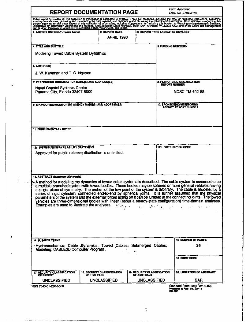
Modeling Towed Cable System Dynamics

6AUTHOR(S)

J. W. Kamman and T. C. Nguyen

7. PERFORMING ORGANIZATION NAME(S) AND ADDRESS(ES) S. PERFORMING ORGANIZATION

Naval Coastal Systems CenterREOTNMRPanama City, Florida 32407-5000 NCSC TM 492-88

9. SPONSORING,1IONITORING AGENCY NAME(S) AND ADDRESS(ES) 10. SPONSORINGMONIrTORINGAGENCY REPORT NUMBER

11. SUPPLEMENTARY NOTES

12m. DISTRIBUTIMNAVANLABILITY STATEMENT 12b. DISTRIBUTION CODE

Approved for public release; distribution is unlimited.

IS. ABSTRACT (Maxhnmm 200 word~s)

/A method for modeling the dynamics of towed cable systems is described. The cable system is assumed to bea multiple branched system with towed bodies. These bodies may be spheres or more general vehicles havinga single plane of symmetry. The motion of the tow point of the system is arbitrary. The cable is modeled by aseries of rigid cylinders connected end-to-end by spherical joints. It is further assumed that the physicalparameters of the system and the external forces acting on It can be lumped at the connecting joints. The towedvehicles are three-dimensional bodies with linear (about a steady-state configuration) time-domain analyses.Examples are used to illustrate the analyses. ~-

14. SUBJECT TERMS 15. NUMBER OF PAGES

-Hydromechanics; Cable Dynamics; Towed Cables; Submerged Cables; 26Mod"W~g CABLE3D Computer Program.

1S. PRICE CODE

17. SECURITY CLASSIFICATION 18. SECURITY CLASSIFICATION 19. SECURITY CLASSIFICATION 20. LIMITATION OF ABSTRACTOF REPORT OF THIS PAGE OF ABSTRACT

UNCLASSIFIED I UNCLASSIFIED I UNCLASSIFIED SARNSN 7540-01-280-6500 Standard Form 298 (Rev. 2-89)

PMsWobmd by ANSt SM. MIS

NCSC TM 492-88

CONTENTS

INTRODUCTION 1

KINEMATICS 2

SYSTEM CONFIGURATION 2

SYSTEM MOTION 4

NONLINEAR EQUATIONS OF MOTION 6

EQUATIONS OF MOTION 6

INTERNAL CABLE FORCES 9

NUMERICAL SOLUTION 12

LINEAR EQUATIONS OF MOTION 12

NUMERICAL SIMULATIONS 14

DISCUSSION 21

REFERENCES 23

, =l . Acoession For(#cW e i NTIS GRA&I

DTIC TAB60 6

Unannounced []Justificat ion-

ByDistribution/

Availability CodesAvail and/or

Dist j Special

NCSC TM 492-88

ILLUSTRATIONS

Fg=hi. Pae

1 Towed Cable System 2

2 Orientation Angles for Cable Links 3

3 Orientation Angles for Towed Vehicles 4

4 General Lumped Mass 8

5 Lumped Mass Attached to a Towed Vehicle 8

6 Towed Vehicle and Attach Point 8

7 Submerged and Partially Submerged CablesDuring a Forward Tow 15

8 Branched Cable Undergoing Forward andCircular Tow 15

9 Cable Motion from Forward to Circular Tow 16

10 Ratio of Sphere Displacement to ExcitationAmplitude 17

1 la Comparison of DYNTOCABS and CABLE3D DropTest Simulations for a 100-ft Cable with a17-lb Sphere on its Free End, 5-Link Model 18

1 lb Comparison of DYNTOCABS and CABLE3D DropTest Simulations for a 100-ft Cable with a17-lb Sphere on its Free End, 10-Link Model 19

1 ilc Comparison of DYNTOCABS and CABLE3D DropTest Simulations for a 100-ft Cable with a17-lb Shpere on its Free End, 15-Link Model 20

12 Execution Time Comparison Between DYNTOCABSand CABLE3D 22

ii

NCSC TM 492-88

INTRODUCTION

Modeling of submerged cable dynamics has been of interest for at least the past 30 years.References 1 through 11 represent a partial listof the many works on this subject covering continuum,finite element, finite segment, and lumped parameter approaches. Reference 12 provides anexcellent survey of the work done prior to 1973.

In a series of recent papers," 13-5 a method was presented based on previously developedgeneral procedures for finite segment modeling of multibody systems.16 17 In that work cables weremodeled by a series of rigid cylinders connected end-to-end by ball-and-socket joints. In particular,in references 14 and 15 the model was partially validated by comparing model predictions withpredictions of linear partial differential equation models 181 9 developed from continuum assumptionsand with experimental data recorded at the Civil Engineering Laboratory at Port Hueneme,California. " As a result of this work, computer programs were developed 2i 12 for the three-dimensional simulation of submerged and partially submerged cable dynamics.

The computer program CABLE3D2 developed at the Naval Coastal Systems Center(NAVCOASTSYSCEN) has been applied to many towed cable systems. However, its utility islimited by extremely long execution times that make the program expensive to use. In 1987NAVCOASTSYSCEN contracted with the University of Alabama to investigate speedimprovements to the CABLE3D code to make it a more viable modeling tool. The results of thisinvestigation are documented in their report.2

For many submerged towed cable systems, the viscous forces acting on the cable are largecompared to the weight forces. Using a lumped parameter model and an analytical approach similarto that in reference 1, it is shown in reference 24 that for these systems (and possibly others whereviscous forces do not dominate) a lumped parameter model is sufficient to model the systemdynamics. Furthermore, it is shown that a substantial increase in execution speed can be achieved(over the computer programs described in references 21 through 23) using this method. With thismotivation, the equations of motion are developed herein using an approach similar to that inreferences I and 24. The lumped parameter model is described in the following paragraphs.

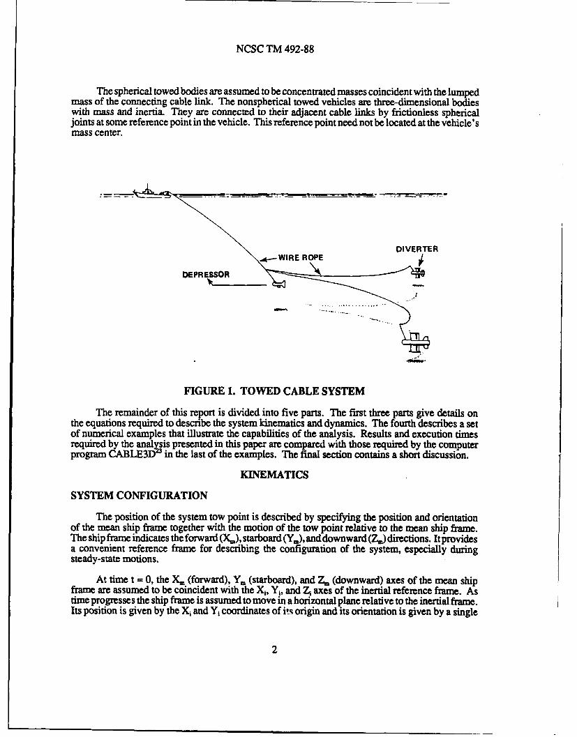
A towed cable system is assumed to be a multiple branched cable system with towed bodies.The system is assumed to be pulled from a single tow point (Figure 1). The cable and its branchesform an open tree system having no closed kinematic chains. Each length of cable may have differentphysical properties, and the towed bodies may be spheres or more general vehicles with a singleplane of symmetry. The motion of the system tow point is arbitrary.

The system is modeled using discrete elements. This allows straightforward formulation ofthe equations of motion for systems with branches and allows physical parameters to be changedfrom element to element. Moreover, the use of simple elements simplifies the solution process.

The cable is modeled by a series of rigid links connected by frictionless spherical joints. Themasses of the links are concentrated half at each of their ends, the connecting joints of the system.All fluid drag, added mass, weight, and buoyancy forces are also concentrated at the connectingjoints. Hence, the cable links are two-force members, carrying forces only along their length. Thelinks are also assumed to be small enough so that the forces acting on them are approximatelyuniform over their length.

NCSC TM 492-88

The spherical towed bodies are assumed to be concentrated masses coincident with the lumpedmass of the connecting cable link. The nonspherical towed vehicles are three-dimensional bodieswith mass and inertia. They are connected to their adjacent cable links by frictionless sphericaljoints at some reference point in the vehicle. This reference point need not be located at the vehicle'smass center.

*.- IRE OPEDIVERTER

DEPRESSOR

FIGURE 1. TOWED CABLE SYSTEM

The remainder of this report is divided into five parts. The first three parts give details onthe equations required to describe the system kinematics and dynamics. The fourth describes a setof numerical examples that illustrate the capabilities of the analysis. Results and execution timesrequired by the analysis presented in this paper are compared with those required by the computerprogram CABLE3D in the last of the examples. The final section contains a short discussion.

KINEMATICS

SYSTEM CONFIGURATION

The position of the system tow point is described by specifying the position and orientationof the mean ship frame together with the motion of the tow point relative to the mean ship frame.The ship frame indicates the forward (X.), starboard (Y.), and downward (Z) directions. It providesa convenient reference frame for describing the configuration of the system, especially duringsteady-state motions.

At time t = 0, the X. (forward), Y. (starboard), and Z. (downward) axes of the mean shipframe are assumed to be coincident with the X,, Y, and Z axes of the inertial reference frame. Astime progresses the ship frame is assumed to move in a horizontal plane relative to the inertial frame.Its position is given by the X, and Y coordinates of it, origin and its orientation is given by a single

2

NCSC TM 492-88

turning angle v1 measured as positive when the ship is in a starboard turn. The orientation of themean ship frame (M) can be related to the orientation of the inertial reference frame (R) throughthe following transformation matrix:

S(R,M) = C(1)

The configuration of the rest of the towed cable system at any instant of time is described bya sequence of orientation angles measured relative to the mean ship frame. The orientation of eachcable link is given by two angles and the orientation of each towed vehicle is given by three angles.Since the mass and external forces acting on a towed sphere are lumped with the mass at the endof its connecting cable link, no additional angles are needed for them. Hence, for a model with atotal of NC cable links and NT towed bodies, there are 2NC + 3NT total angles needed to definethe configuration of the system. This is also the number of degrees-of-freedom of the model.

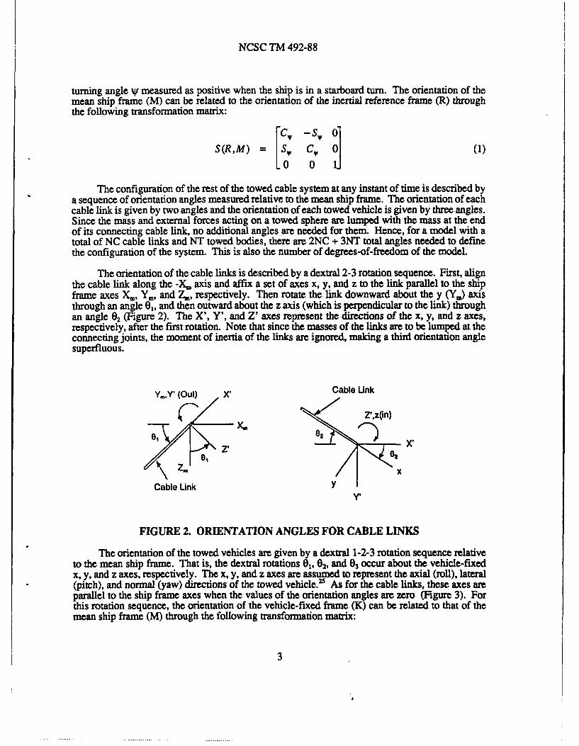
The orientation of the cable links is described by a dextral 2-3 rotation sequence. First, alignthe cable link along the -X, axis and affix a set of axes x, y, and z to the link parallel to the shipframe axes X., Y., and Z., respectively. Then rotate the link downward about the y (Y.i) axisthrough an angle 01, and then outward about the z axis (which is perpendicular to the link) throughan angle 02 (Figure 2). The X', Y', and Z' axes represent the directions of the x, y, and z axes,respectively, after the first rotation. Note that since the masses of the links are to be lumped at theconnecting joints, the moment of inertia of the links are ignored, making a third orientation anglesuperfluous.

Y..Y' (Out) X' Cable Unk

ZZ'z(in)

Cable Link Y 'y,

FIGURE 2. ORIENTATION ANGLES FOR CABLE LINKS

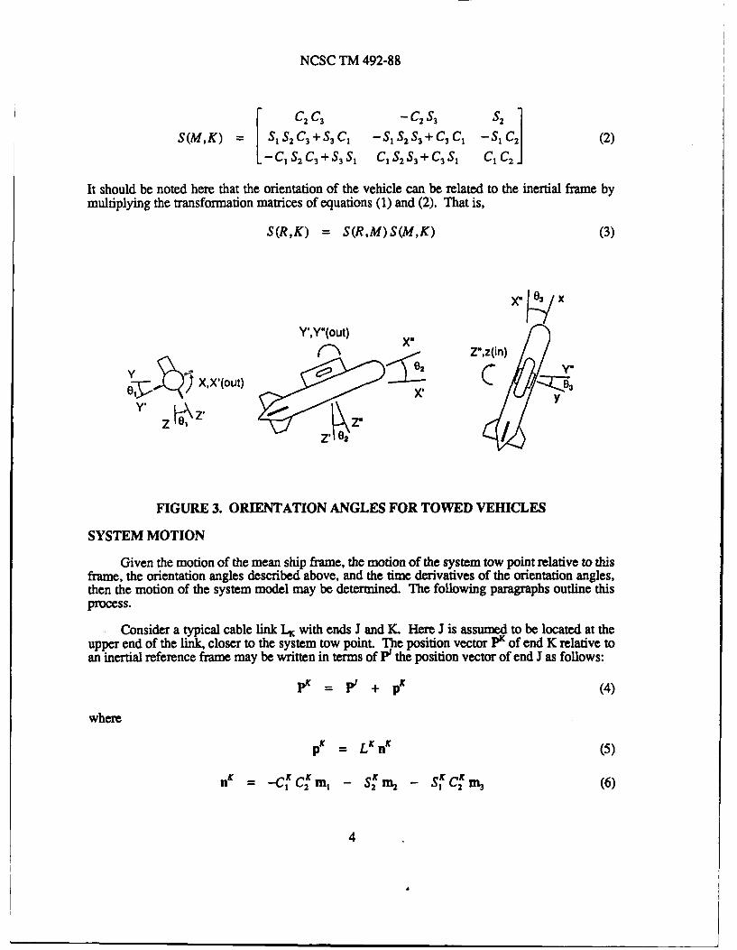
The orientation of the towed vehicles are given by a dextral 1-2-3 rotation sequence relativeto the mean ship frame. That is, the dextral rotations 0,02, and 03 occur about the vehicle-fixedx, y, and z axes, respectively. The x, y, and z axes are assumed to represent the axial (roll), lateral(pitch), and normal (yaw) directions of the towed vehicle.,5 As for the cable links, these axes axeparallel to the ship frame axes when the values of the orientation angles are zero (Figure 3). Forthis rotation sequence, the orientation of the vehicle-fixed frame (K) can be related to that of themean ship frame (M) through the following transformation matrix:

3

NCSC TM 492-88

C2 C3 -C2S3 S2 1S(M, K) = S2C3+S3C1 -S 1 S2 S3 +C 3 C -Sic 1 (2)

L-c, s2C3+s3s, C, s2s 3 + C3s1 S1 C 2 c

It should be noted here that the orientation of the vehicle can be related to the inertial frame bymultiplying the transformation matrices of equations (1) and (2). That is,

S(R,K) = S(R,M) S(M,K) (3)

X" /x

YY*(Out) X

Z*,z~in)

LX y"

Y',Ylout i''01

Z F2

FIGURE 3. ORIENTATION ANGLES FOR TOWED VEHICLES

SYSTEM MOTION

Given the motion of the mean ship frame, the motion of the system tow point relative to thisframe, the orientation angles described above, and the time derivatives of the orientation angles,then the motion of the system model may be determined. The following paragraphs outline thisprocess.

Consider a typical cable link LK with ends J and K. Here J is assumed to be located at theupper end of the link, closer to the system tow point. The position vector P" of end K relative toan inertial reference frame may be written in terms of V the position vector of end J as follows:

P -F + pK (4)

where

L K Kn (5)

= - MCC in - SK 2 M2 - SKC M3 (6)

4

NCSC TM 492-88

where the SK and C1 represent the sin (0) and the cos (0), respectively, and the n (i = 1, 2, 3)represent unit vectors fixed in the mean ship frame. Note here that using equation (4) and P0 theposition vector of the system tow point, the position vectors of the end points of all the cable linkscan be determined.

Equation (4) may now be differentiated to give the velocities and accelerations of the endsof the links as follows:

= V + (7)

A' = A + pK (8)

where

pK = p 61 + Pv K(9)

p = pK + pK +pOK + aj (10)

and where piK and pK represent the partial derivatives of pK with respect to Of (i 1, 2) and i,respectively, and the dots represent time differentiation. Explicit forms for AK and V" may be foundby performing the necessary differentiations of p as given by equations (5) and (6). In the numericalprocedure presented in the sequel explicit forms are required only for pK. Regarding notation,repeated subscripts (such as i in the above equations) represent a sum over the range of that index.This notation will be used consistently throughout the remainder of this paper.

The above equations provide components of the positions, velocities, and accelerations ofthe lumped masses as a function of the ship motion, the cable link angles, and the link anglederivatives. Later in this analysis, it will be necessary to calculate the second derivatives of thelink angles from the acceleration components. To this end, noting that p pis zero, it was shownin reference 24 that:

[A -' -p~r-iji] .pf (11)gK [A - f * _pgA.p p

pgK piK(

for i = 1, 2. Hence, given the lumped mass accelerations components, the link angles, and the linkangle derivatives, the second derivatives of the link angles can be calculated. Note here again thatthere is a sum in equation (11) over the range of the repeated index j from 1 to 2.

Consider next a typical towed vehicle. Given the orientation angles and their time derivatives(1-2-3 rotation sequence as presented earlier) for the towed vehicle, the angular velocity and angularacceleration of the vehicle may be written as follows:'

w = oibj and * = 6ibi (12)

where the bi are unit vectors fixed in the vehicle and

5

NCSC TM 492-88

= c2 c 3 1 + + (S, S3 - C1 S2 C3) (13)

S= .-C2 36 + C3 06 + 1/(S, C3 +C, S2 S3 ) (14)

(3= S2O + OK + C1 ,jC, (15)

The velocity of the mass center of the vehicle can then be determined as follows:

VX = VI + wxpK (16)

where V' represents the velocity of J the lumped mass at the end of the adjacent cable link and pK

represents the position vector of the mass center of the vehicle relative to J.

Equations (13) through (15) may also be inverted to give26

0 = C3 [0- (S S3 - C S2 C)] / C2 - S3 [02- * (S C3 + C1 S2 S)] / C2 (17)

OK = S o-' (S - C1 S2 C3)] + C3 [( 2- j (S C3 + C1ss) (18)

63K = ( c C1 C2 - S2 C3 101 (S S3 - C1 S2 )/ C2

+ S2 S3 [-i (S C3 + C S2 S)]/ C2 (19)

These equations may now be differentiated to give explicit equations for calculating the secondderivatives of a vehicle's orientation angles given the components of its angular acceleration vector(along the vehicle-fixed directions), the orientation angles and their first derivatives, and the angularmotion of the mean ship frame.

NONLINEAR EQUATIONS OF MOTION

EQUATIONS OF MOTION

The equations of motion of the system model can be found by applying Newton's law ofmotion to each of the model's components. In general, these eouations may be written as follows:

M= or = A~ (20)

where the yK represents 4 (i = 1, 2, 3) the inertial acceleration components of the lumped masses

and 4 (i = 1, 2, 3) and 6wf (i = 1, 2, 3) the mass center acceleration components and angularacceleration components of the towed vehicles in the vehicle-fixed frame. The range of thesubscripts i and j in equation (20) are thus from 1 to 3 for lumped masses and from 1 to 6 for towedvehicles, and the definitions of MUK and ff depend, of course, on the particular model component.

Note here also that A in equation (20) represents the inverse of matrix M4K.

6

NCSC TM 492-88

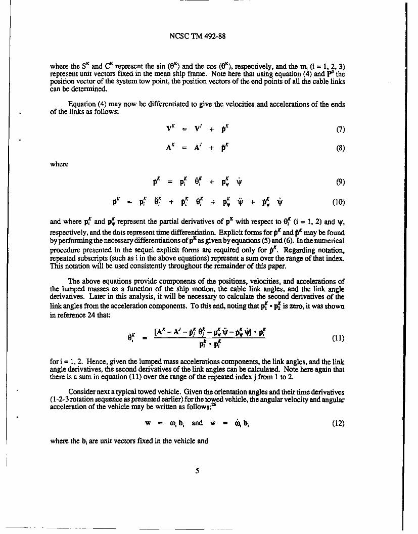
For the general lumped mass shown in Figure 4 we have

+ M + A + A + A H) S# - Akn! - Y2An n/njH(i,j=1,2,3)(21)

f = -t n i + + I + (Q+Q).i,(i= 1 ,2 , 3 ) (22)H

where ii represent unit vectors fixed in an inertial reference frame and 8 represents the standardKronecker delta symbol.V The entries in the symmetric mass matrix M? include mL the mass ofthe sphere, mK half the total mass of all the adjacent cable links, AL the added mass of the sphere,A" and AH, (H = KI .... , K.) half the added masses of the adjacent cable links, and n; (J = K, K1,.... K.) the inertial components of the unit vectors n' (which are parallel to the links). The valuesof the added mass entries are taken to be:

AL= CM p VL (23)

A = -1 CM pV (24)2

where CM is the added mass coefficient, p is the density of the fluid, and VL and V3 (J = K, K.... K.) denote the volumes of the sphere and the adjacent cable links, respectively. Note that Aand A3 are defined as in references 5 and 13 except for the link added masses that are multipliedby a factor of one-half for distribution to the lumped masses. The vector if includes e the internalcable tensions, QL the resultant of the drag, buoyancy, and weight forces acting on the sphere, andQK half the resultant of the drag, buoyancy, and weight forces acting on all adjacent cable links.Note that these forces are also taken as presented in references 5 and 13, with drag forces assumedconstant over the cable links. As with the mass and added mass distributions, the forces on thecable links are all distributed half at each end.

Consider next a lumped mass attached to a towed vehicle in Figure 5. In this case the entriesM f nd f become:

M = (o+A K)84 - A nf nj (i,j=1,2,3) (25)

if = -tKnK + S(R,L)U tL + (QK) .i (i = 1,2,3) (26)

where, as before, mK represents half the mass and AK represents half the added mass on the adjacentcable link K, nf represents the inertial components of a unit vector parallel to the link K, ti representsthe force in link K, QK represents half the resultant of the fluid drag, buoyancy, and wei-ht forceson link K, and tL represents the components of the force acting on the lumped mass due to theadjacent towed body along vehicle-fixed directions. The matrix S(RL) is the transformation matrixrelating the orientation of towed vehicle L to the inertial reference frame.

7

NCSC TM 492-88

J2J

J2

Link KnKI L Lik J?

K1 K

T (due to towed vehicle)K,

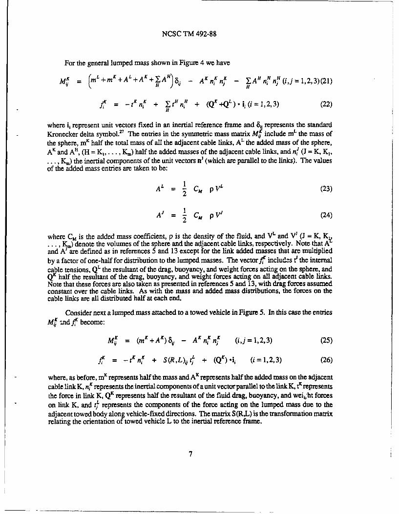
FIGURE 4. GENERAL LUMPED MASS FIGURE 5. LUMPED MASS ATTACHEDTO A TOWED VEHICLE

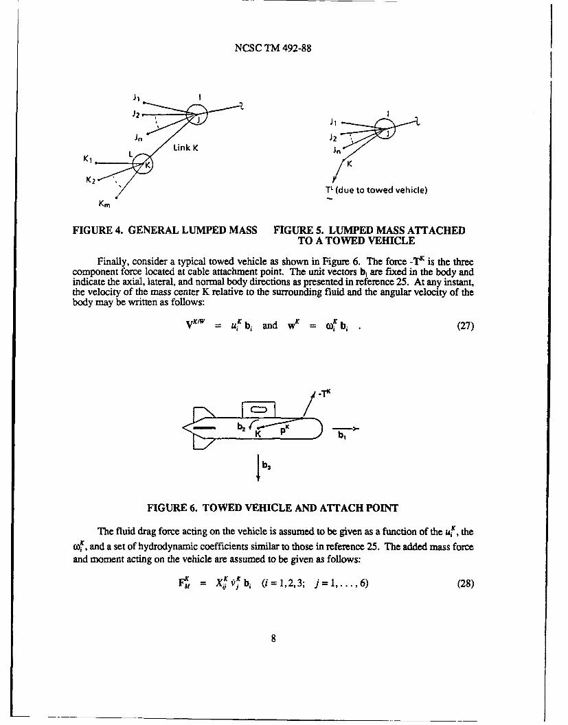
Finally, consider a typical towed vehicle as shown in Figure 6. The force - 7 is the threecomponent force located at cable attachment point, The unit vectors bi are fixed in the body andindicate the axial, lateral, and normal body directions as presented in reference 25. At any instant,the velocity of the mass center K relative to the surrounding fluid and the angular velocity of thebody may be written as follows:

VK1' = u b, and wK = b, (27)

K TK

Ib3FIGURE 6. TOWED VEHICLE AND ATTACH POINT

The fluid drag force acting on the vehicle is assumed to be given as a function of the ui1, the

o , and a set of hydrodynamic coefficients similar to those in reference 25. The added mass forceand moment acting on the vehicle are assumed to be given as follows:

1, = XK v'bj (i=1,2,3; j=l,...,6) (28)

8

NCSC TM 492-88

= Nurb, (i=1,2,3; j=l,...,6) (29)

where

viK = uf (i=1,2,3) (30)

vf = COK_, (i=4,5,6) (31)

and the X4K and N are a specified set of coefficients again similar to those in reference 25.

Using this notation, Mj andfK of equation (20) for a towed vehicle may be written as follows:

j= mK8 0 - X, (i,j=1,2,3) (32)

Mij = -X4 (i=1,2,3; j=4,5,6) (33)

= -N,-,i (i=4,5,6; j=1,2,3) (34)

MiK = [= 6

M -3.J-3 -N3 (i,j=4,5,6) (35)

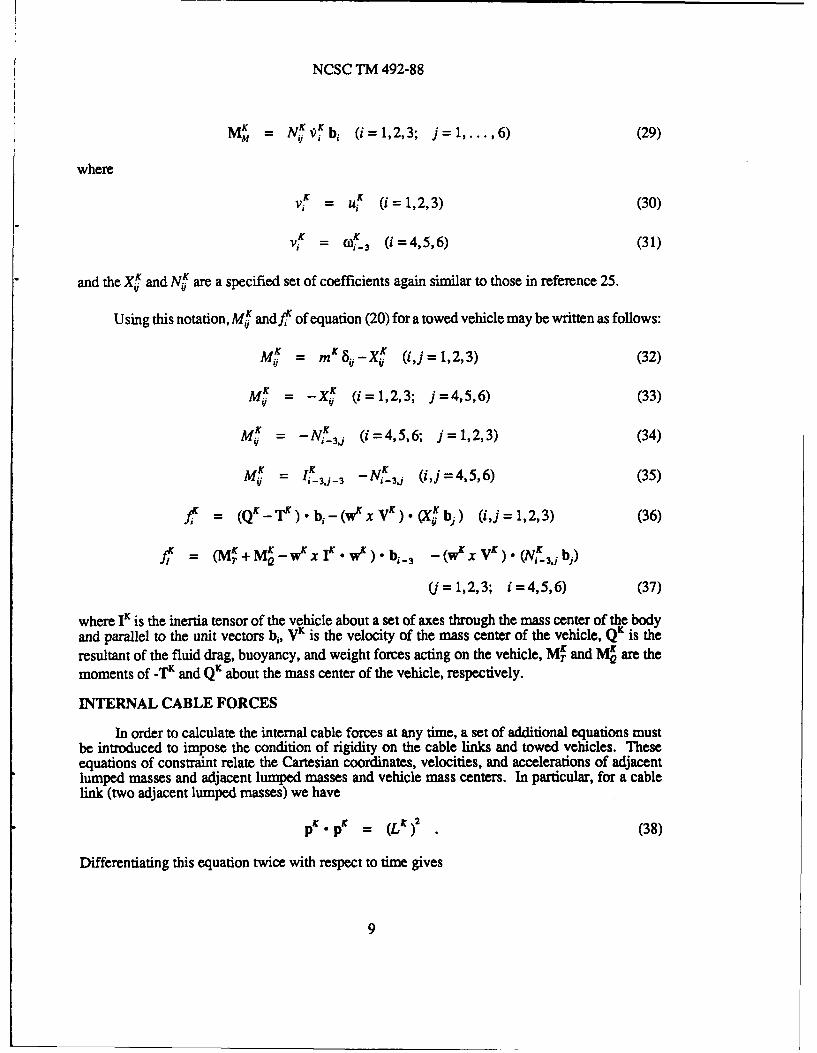
fK = (QK-TK).b,- (wxVK).(Xu bj) (i,j=1,2,3) (36)

f = (MK+M WKxIK.wK) bi_3 -(wK xx V). (N _3Jbi)

(=1,2,3; i=4,5,6) (37)

where IK is the inertia tensor of the vehicle about a set of axes through the mass center of the bodyand parallel to the unit vectors bi, VK is the velocity of the mass center of the vehicle, QK is theresultant of the fluid drag, buoyancy, and weight forces acting on the vehicle, Mr and M are themoments of -TK and QK about the mass center of the vehicle, respectively.

INTERNAL CABLE FORCES

In order to calculate the internal cable forces at any time, a set of additional equations mustbe introduced to impose the condition of rigidity on the cable links and towed vehicles. Theseequations of constraint relate the Cartesian coordinates, velocities, and accelerations of adjacentlumped masses and adjacent lumped masses and vehicle mass centers. In particular, for a cablelink (two adjacent lumped masses) we have

p . pK = (L )2 (38)

Differentiating this equation twice with respect to time gives

9

NCSC TM 492-88

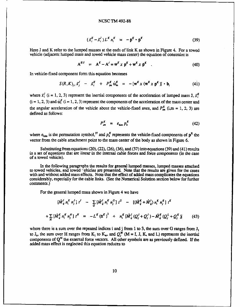
_= (39)

Here J and K refer to the lumped masses at the ends of link K as shown in Figure 4. For a towed

vehicle (adjacent lumped mass and towed vehicle mass center) the equation of constraint is

A'"' = A'_A"= *K x PK+WKXt (40)

In vehicle-fixed component form this equation becomes

S(R,K)J1 9j - 4K + P , =-[w" x(w'rxpX)] bi (4i)

where Y! (i = 1, 2, 3) represent the inertial components of the acceleration of lumped mass J, 4f(i = 1, 2, 3) and 6!K (i = 1, 2, 3) represent the components of the acceleration of the mass center andthe angular acceleration of the vehicle about the vehicle-fixed axes, and PK (im = 1, 2, 3) aredefined as follows:

. = e,, Pk (42)

where ek is the permutation symbol,2 and pK represents the vehicle-fixed components of pK thevector from the cable attachment point to the mass center of the body as shown in Figure 6.

Substituting from equations (20), (22), (26), (36), and (37) into equations (39) and (41) resultsin a set of equations that are linear in the internal cable forces and force components (in the caseof a towed vehicle).

In the following paragraphs the results for general lumped masses, lumped masses attachedto towed vehicles, and towed -'ehicles are presented. Note that the results are given for the caseswith and without added mass effects. Note that the effect of added mass complicates the equationsconsiderably, especially for the cable links. (See the Numerical Solution section below for furthercomments.)

For the general lumped mass shown in Figure 4 we have

[M'K nfnG] tG _ [(4K~ ~)f tK

+I[K nf njIr ] t -,(I"I) 2 + n[9A ( +Q)-9,(Qj+Q ) (43)

where there is a sum over the repeated indices i and j from 1 to 3, the sum over G ranges from J,to J,, the sum over H ranges from K, to K,,, and Qr (M = , J, K, and L) represents the inertialcomponents of QM the external force vectors. All other symbols are as previously defined. If theadded mass effect is neglected this equation reduces to

10

NCSC TM 492-88

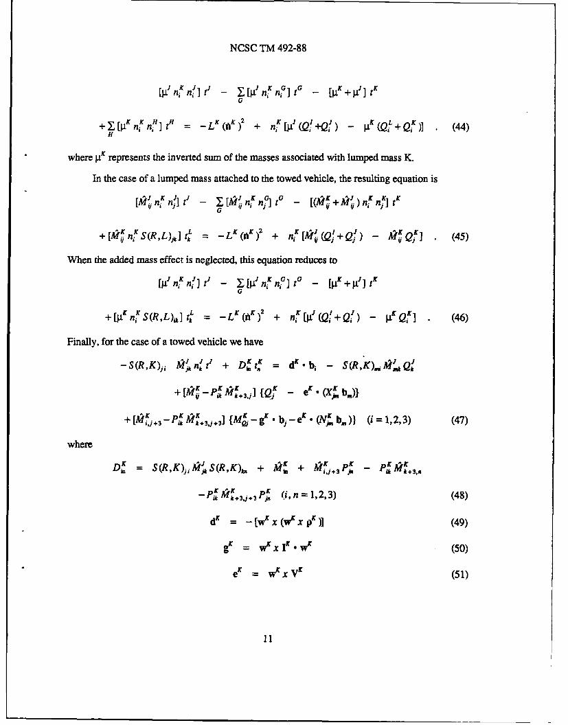
[,,,ht' - n ,,It' - [j +j]t1G

+H[P nK tH = -LK (eK)2 + nK[P(QI:- ) - I.IQL+QK)] (44)

where ? represents the inverted sum of the masses associated with lumped mass K.

In the case of a lumped mass attached to the towed vehicle, the resulting equation is

[n Kn! Wj n [ K n -t [( +M kJnnK] tK

+[~A n[ S(R,L)kI = -L( )2 + # -i ] (45)

When the added mass effect is neglected, this equation reduces to

,:, t- n [d ,,,,[]W -tG + W]tKG

+ [. nK S(R,L),] tk = -LK (AK ) + nK [V (Q[+ Q) _ Q (46)

Finally, for the case of a towed vehicle we have-S(R,K)ji W n? + DK. = dK.bi S

lMfJ] {Qj - eK. (Xj. b)}

+[ijX+3-P 3 + 3IsM .- 9K 'bi - eK (Ni,b,,,)) (i = 1, 2,3) (47)

whereDm = S(R,K)j 1M.S(R,K),, + k!I + ..f-i P+3 -aM.&k+ 3,n

pK

k+3.j+3p (i,n =1,2,3) (48)

d = -[wIx( w KxpV)] (49)

gK = wIxIK wK (50)

e - wKx VK (51)

11

NCSC TM 492-88

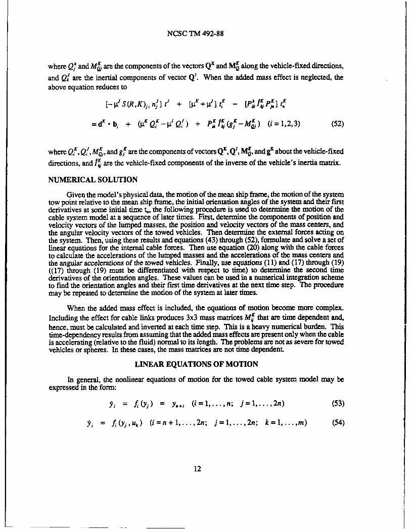
where Qj' and Mi are the components of the vectors QK and M along the vehicle-fixed directions,

and Q' are the inertial components of vector QJ. When the added mass effect is neglected, theabove equation reduces to

[ILS (R, K),,in.'I tj V + eIt - [Pikk , I 1. .

=d. + (KQK-..jQJ) + Pif #gf-M ) (i=1,2,3) (52)

where QK, Q!, M , and gf are the components of vectors QK, Q, M, and g about the vehicle-fixed

directions, and fk are the vehicle-fixed components of the inverse of the vehicle's inertia matrix.

NUMERICAL SOLUTION

Given the model's physical data, the motion of the mean ship frame, the motion of the systemtow point relative to the mean ship frame, the initial orientation angles of the system and their firstderivatives at some initial time to, the following procedure is used to determine the motion of thecable system model at a sequence of later times. First, determine the components of position andvelocity vectors of the lumped masses, the position and velocity vectors of the mass centers, andthe angular velocity vectors of the towed vehicles. Then determine the external forces acting onthe system. Then, using these results and equations (43) through (52), formulate and solve a set oflinear equations for the internal cable forces. Then use equation (20) along with the cable forcesto calculate the accelerations of the lumped masses and the accelerations of the mass centers andthe angular accelerations of the towed vehicles. Finally, use equations (11) and (17) through (19)((17) through (19) must be differentiated with respect to time) to determine the second timederivatives of the orientation angles. These values can be used in a numerical integration schemeto find the orientation angles and their first time derivatives at the next time step. The proceduremay be repeated to determine the motion of the system at later times.

When the added mass effect is included, the equations of motion become more complex.

Including the effect for cable links produces 3x3 mass matrices Mf. that are time dependent and,hence, must be calculated and inverted at each time step. This is a heavy numerical burden. Thistime-dependency results from assuming that the added mass effects are present only when the cableis accelerating (relative to the fluid) normal to its length. The problems are not as severe for towedvehicles or spheres. In these cases, the mass matrices are not time dependent.

LINEAR EQUATIONS OF MOTION

In general, the nonlinear equations of motion for the towed cable system model may beexpressed in the form:

S' = f 1(Yj) = Y.+i (i=l,...,n; j=l,...,2n) (53)

i = f,(y,,uk) (i=n+l,...,2n; j=l,...,2n; k=l,...,m) (54)

12

NCSC TM 492-88

where y (i = 1,... , n) represent the orientation angles relative to the mean ship frame of the cablelinks and towed vehicles of the system. y, (i = n + 1 ... , 2n) represent the first derivatives ofthese angles, and u, (k = 1, .... , m) represent a set of external inputs, such as tow point motion andcontrol surface motions on the towed vehicles. During steady forward or steady turning motionand in the absence of external disturbances, the system can exhibit steady-state equilibrium positions.In these situations, the orientation angles relative to the mean ship frame remain constant. Theseangles may be found by solving the n nonlinear algebraic equations

fR+,(yj,,y+j,,.=O) = 0 (i,j=l,...,n) (55)

where yj, and y, +j,, (j = 1, ... n) represent the equilibrium values of the orientation angles of thesystem and their time derivatives, respectively.

To describe motions of the system that result from small disturbances to the state vector y orto the external input vector u, the nonlinear equations of motion ((53) and (54)) can be linearizedabout the equilibrium configuration. To this end, introduce a perturbation vector z to the equilibriumstate vector y, and a perturbation vector v to the equilibrium external input vector u. so that

y = y, + z (i'-1,...,2n) (56)

Uk = UA + Vk (k=l,...,m) (57)

Substituting these values into the nonlinear equations of motion, expanding in a Taylor Series aboutthe equilibrium configuration, and omitting terms of second for higher order in the perturbations zand vk results in the equations

ii= Az, + Bavk (58)

where

= (afa/ y) (59)

B = (afj / auk). (60)

Here the subscript e on the partial derivatives indicates that they are evaluated at the equilibriumconfiguration. Since the first n equations (53) are simply definitions of the state vector y, the firstn rows of the A and B matrices take on the special values

A = 0 (ij=l,...,n) (61)

Ai.,=+ 8# (i,j=l,...,n) (62)

Ba = 0 (i=l,...,n; k=l,...,m) (63)

13

NCSC TM 492-88

where, as before, 8,j represents the standard Kronecker delta symbol.

The nontrivial entries in the matrices may be approximated using finite differences. In thiswork a second-order central difference is used so that the entries are calculated as follows:

f (y. + dyj , u,) - f (y,-dyj,u ) (64)

2dy(

f (y,,u,+duk) - f (y,,u-du ) (65)Bik = 2 duk (65)

where dy, and duk represent small increments in y,, and uk; dyj represents the 2n-vector of increments

(0 ... , dyj, 0 ... , 0) and dul represents the m-vector of increments (0 .... , 0, duk, 0, ... , 0).The nonzero increments dy and duk occur in the jb and ke ' entries of dyj and dUk, respectively. Notethat since the steady-state motion is stationary, the matrices A and B are constant matrices.

Equation (58) represents a set of first-order linear system of equations in the perturbations zand v. They are useful for studying towed system stability, sensitivity to change of input state v,and control analysis. 2

NUMERICAL SIMULATIONS

The procedures outlined in the previous sections of this report have been incorporated into acomputer program NCSC -DYNTOCABS (Naval Coastal Systems Center -DYNamics of TOwedCABle Systems). The following paragraphs outline a set of examples that serve to illustrate thecapabilities of the program. Examples of nonlinear, linear, and steady-state analyses are presented.The final example compares the results and execution times of DYNTOCABS with the programCABLE3D. 23

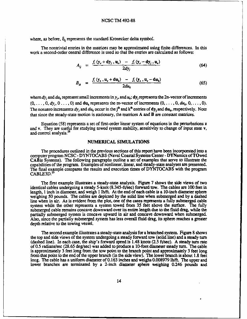
The first example illustrates a steady-state analysis. Figure 7 shows the side views of twoidentical cables undergoing a steady 5-knot (8.345-ft/sec) forward tow. The cables are 100 feet inlength, 1 inch in diameter, and weigh 1 lb/ft. At the end of each cable is a 10-inch diameter sphereweighing 50 pounds. The cables are depicted by the solid line when submerged and by a dashedline when in air. As is evident from the plot, one of the cases represents a fully submerged cablesystem while the other represents a system towed from 35 feet above the surface. The fullysubmerged cable remains concave downward over its entire length due to the fluid drag, while thepartially submerged system is concave upward in air and concave downward when submerged.Also, since the partially submerged system has less overall fluid drag, its sphere reaches a greaterdepth relative to the towing vessel.

The second example illustrates a steady-state analysis for a branched system. Figure 8 showsthe top and side views of the system undergoing a steady forward tow (solid line) and a steady turn(dashed line). In each case, the ship's forward speed is 1.48 knots (2.5 ft/sec). A steady turn rateof 0.5 radians/sec (28.65 deg/sec) was added to produce a 10-foot diameter steady turn. The cableis approximately 3 feet long from the tow point to the branch point and approximately 3 feet longfrom that point to the end of the upper branch (in the side view). The lower branch is about 1.8 feetlong. The cable has a uniform diameter of 0.163 inches and weighs 0.008979 lb/ft. The upper andlower branches are terminated by a 2-inch diameter sphere weighing 0.246 pounds and

14

NCSC TM 492-88

0.492 pounds, respectively. Figure 8 shows that the steady-state configuration of the cable systemduring the steady turn remains inside the 10-foot diameter circle prescribed by the ship motion andis deeper than the steady-state configuration of the corresponding forward tow.

SIDE VIEW°I

0 ,

I-

1u 40

J

ILU0.

C.o

X RELATIVE TO SHIP (FT)

FIGURE 7. SUBMERGED AND PARTIALLY SUBMERGED CABLESDURING A FORWARD TOW

TOP VIEW SIDE VIEW

-. O &"I.S

0 a .0

0 0(8 -2.0

.5.

-2.0 *' * .

-4.0

X 4.0SLi-S.S I L .

... ..... . . . . . . . . . .h

.6 S -4 .3 -l .0 0 I 1 3 4 1 S

Y RELATIVE TO SHIP (FT) X RELATIVE TO SHIP (FT)

FIGURE 8. BRANCHED CABLE UNDERGOING FORWARD AND CIRCULAR TOW

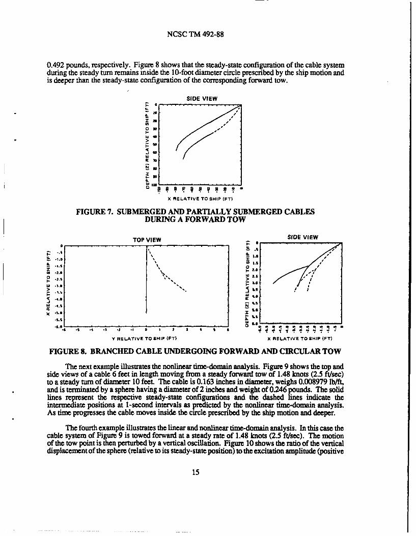
The next example illustrates the nonlinear time-domain analysis. Figure 9 shows the top andside views of a cable 6 feet in length moving from a steady forward tow of 1.48 knots (2.5 ft/sec)to a steady turn of diameter 10 feet. The cable is 0.163 inches in diameter, weighs 0.008979 lb/ft,and is terminated by a sphere having a diameter of 2 inches and weight of 0.246 pounds. The solidlines represent the respective steady-state configurations and the dashed lines indicate theintermediate positions at -second intervals as predicted by the nonlinear time-domain analysis.As time progresses the cable moves inside the circle prescribed by the ship motion and deeper.

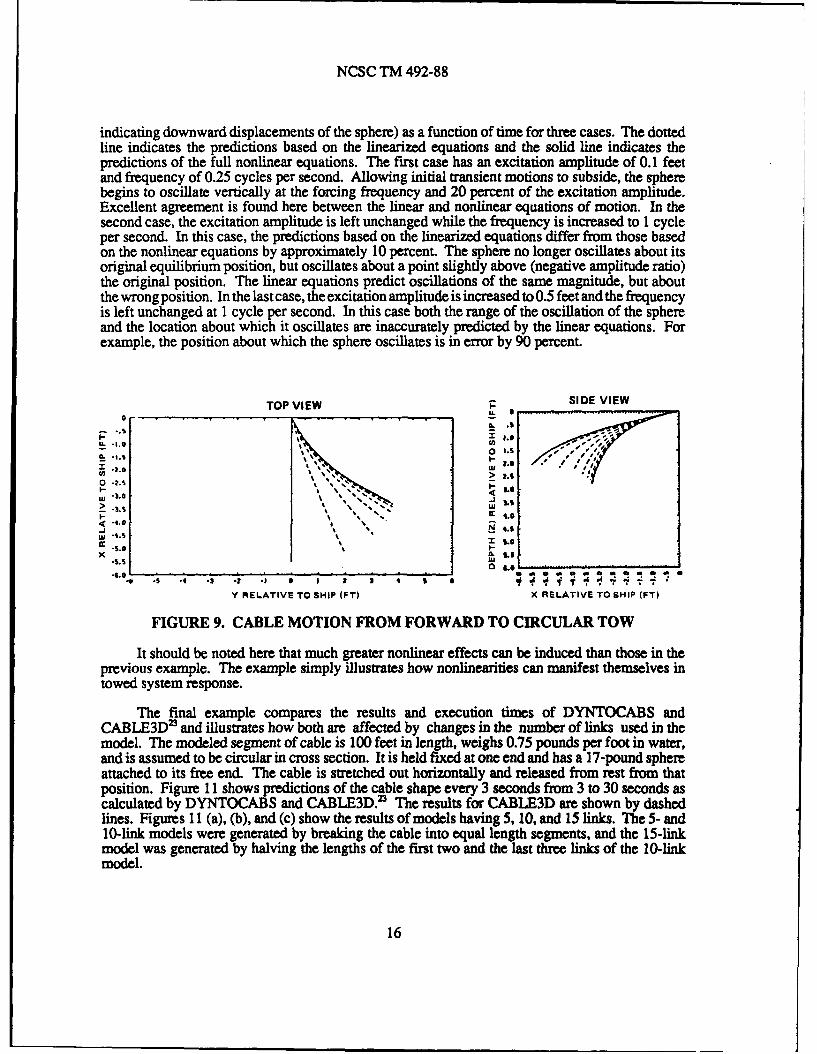
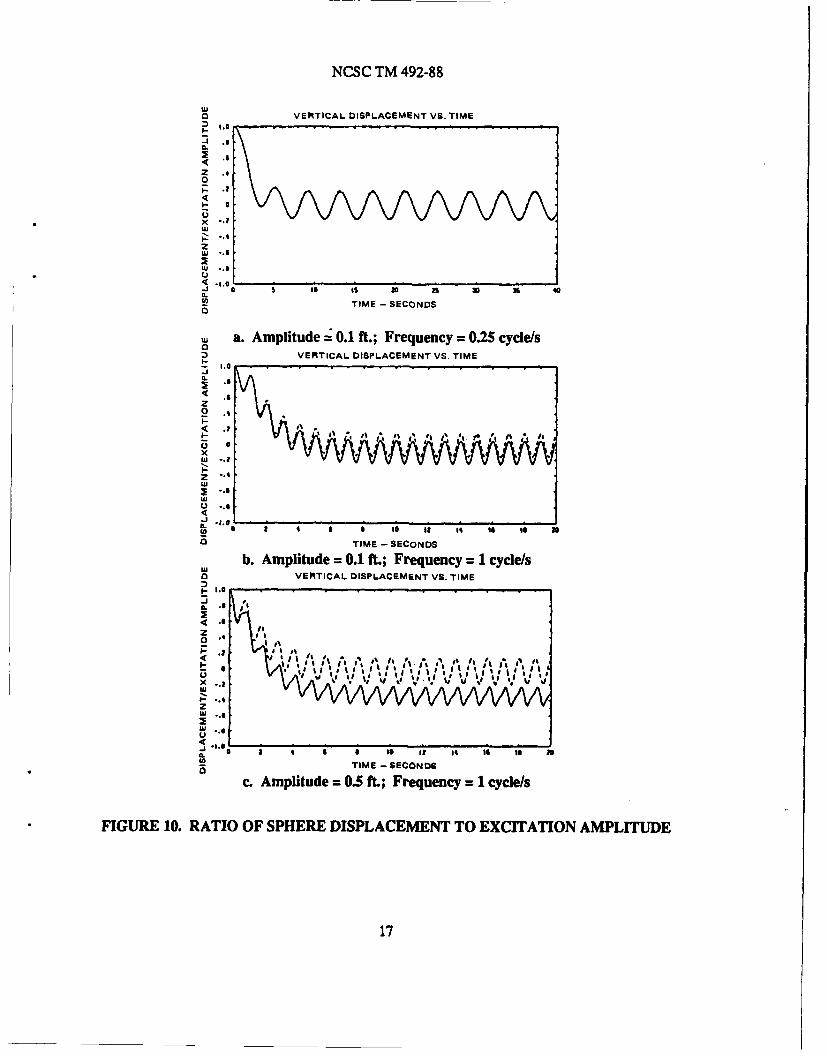
The fourth example illustrates the linear and nonlinear time-domain analysis. In this case thecable system of Figure 9 is towed forward at a steady rate of 1.48 knots (2.5 ft/sec). The motionof the tow point is then perturbed by a vertical oscillation. Figure 10 shows the ratio of the verticaldisplacement of the sphere (relative to its steady-state position) to the excitation amplitude (positive

15

NCSC TM 492-88

indicating downward displacements of the sphere) as a function of time for three cases. The dottedline indicates the predictions based on the linearized equations and the solid line indicates thepredictions of the full nonlinear equations. The first case has an excitation amplitude of 0.1 feetand frequency of 0.25 cycles per second. Allowing initial transient motions to subside, the spherebegins to oscillate vertically at the forcing frequency and 20 percent of the excitation amplitude.Excellent agreement is found here between the linear and nonlinear equations of motion. In thesecond case, the excitation amplitude is left unchanged while the frequency is increased to 1 cycleper second. In this case, the predictions based on the linearized equations differ from those basedon the nonlinear equations by approximately 10 percent. The sphere no longer oscillates about itsoriginal equilibrium position, but oscillates about a point slightly above (negative amplitude ratio)the original position. The linear equations predict oscillations of the same magnitude, but aboutthe wrongposition. In the last case, the excitation amplitude is increased to 0.5 feet and the frequencyis left unchanged at 1 cycle per second. In this case both the range of the oscillation of the sphereand the location about which it oscillates are inaccurately predicted by the linear equations. Forexample, the position about which the sphere oscillates is in error by 90 percent.

TOP VIEW SIDE VIEW

0 --- -----------

I- .,.• -..1- 2. ss I

w ..O , ,, '. u

" -Z,

IS

X L 9.

• S.C S . . . .. . . . . .. . . . . . .

-6 * 4 -s1 -3 2 .3 0 I 2 1 6

Y RELATIVE TO SHIP (FT) X RELATIVE TO SHIP (FT)

FIGURE 9. CABLE MOTION FROM FORWARD TO CIRCULAR TOW

It should be noted here that much greater nonlinear effects can be induced than those in theprevious example. The example simply illustrates how nonlinearities can manifest themselves intowed system response.

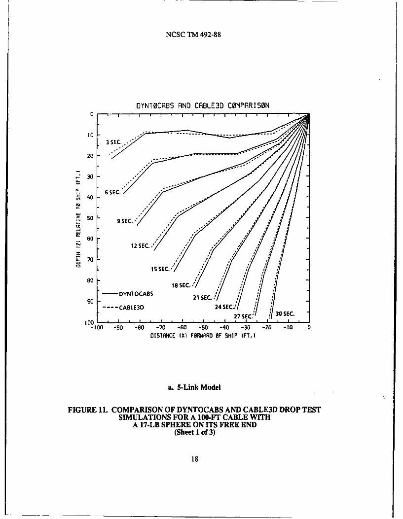
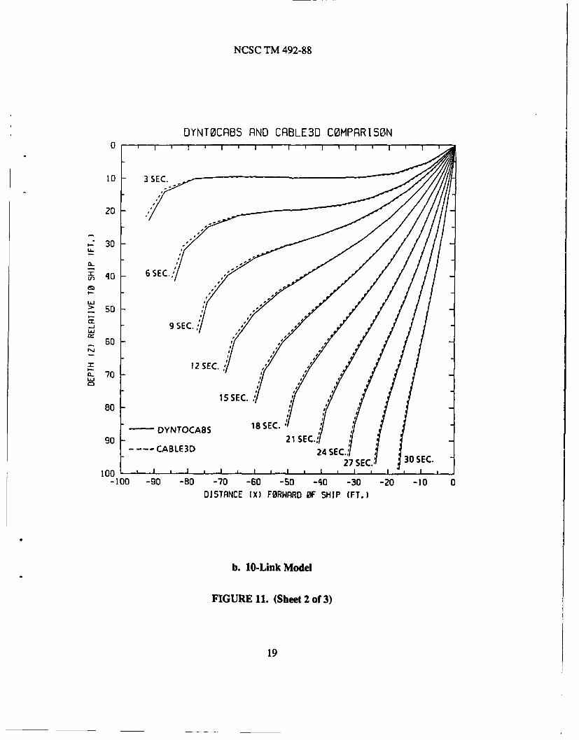
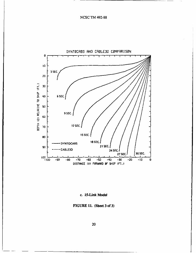
The final example compares the results and execution times of DYNTOCABS andCABLE3D2 and illustrates how both are affected by changes in the number of links used in themodel. The modeled segment of cable is 100 feet in length, weighs 0.75 pounds per foot in water,and is assumed to be circular in cross section. It is held fixed at one end and has a 17-pound sphereattached to its free end. The cable is stretched out horizontally and released from rest from thatposition. Figure 11 shows predictions of the cable shape every 3 seconds from 3 to 30 seconds ascalculated by DYNTOCABS and CABLE3D.2 The results for CABLE3D are shown by dashedlines. Figures 11 (a), (b), and (c) show the results of models having 5, 10, and 15 links. The 5- and10-link models were generated by breaking the cable into equal length segments, and the 15-linkmodel was generated by halving the lengths of the first two and the last three links of the 10-linkmodel.

16

NCSC TM 492-88

a VERTICAL DISPLACEMENT VS. TIME

0

0

Ij-. 60.2'U

ILJ s*.Is6 i 0 6 4

TIME - SECONDS

a. Amplitude =0.1 ft.; Frequency =0.25 cycletsVERTICAL DISPLACEMENT VS. TIME

I-

21 a.

o IE- EOD

.

4 .6 o t I0zIE-EO Do b.Apiue0. t;Feuec yl/

- VETIA DIPAEMN'S.TM

D

Z I

<--.l itft ot11

Uj

0 TIME -SECONDSc. Amplitude = .5 ft.; Frequency I cycle/s

FIGURE 10. RATIO OF SPHERE DISPLACEMENT TO EXCITATION AMPLITUDE

17

NCSC TM 492-88

OYNTOCRBS AND CRBLE3D COMPARISON

10

~30U-

9z 6 SEC.incq

uJ

60

CL 70

8018SC

-0 DYNTOCABS 1SC

-- CABLE3D24SC.

27SEC. 30 SEC.

-100 -90 -80 -70 -60 -50 -40 -30 -20 -10 0DISTANCE MX FORWARDO F SHIP (FT.)

a. 5-Link Model

FIGURE 11. COMPARISON OF DYNTOCABS AND CABLE3D) DROP TESTSIMULATIONS FOR A 100-FT CABLE WITH

A 17-LB SPHERE ON ITS FREE END(Sheet 1 of 3)

18

NCSC TM 492-88

OYNTOCRBS RNO CRBLE3D COMPRRISO~N

250

60

50

9 0t4--CBL3

DYNTb.B 10-in Model

FIUR 21. (SEC.o.3

CABLE 24 EC19

NCSC TM 492-88

DYNTOCRBS FiND CRBLE30 COMPRRISON

10

20

.- 30

u.j

: 50

-J

60

S70u.j

80

DYNTOCABS18SC

90 CABLE3D 21SC 4 SEC.

-30 -90 -80 -70 -60 -50 -40 -30 -20 -10 0DISTANCE (XI FORWARD OF SHIP (FT.)

c. 15-Link Model

FIGURE 11. (Sheet 3 of 3)

20

NCSC TM 492-88

It is evident from a comparison of Figures 11 (a) through (c) that 5 links is insufficient tomodel the curvature of the cable as it drops. Although much smoother than the 5-link model, the10-link model still has difficulty near the fixed and free ends. Moreover, it should be noted thatthe predictions of the 5- and 10-link models lagged behind those of the 15-link model which appearsto adequately describe the system dynamics. In fact, further refined 20- and 30-link models predictednearly identical results. Finally, although some differences are apparent, the results ofDYNTOCABS and CABLE3D agree closely.

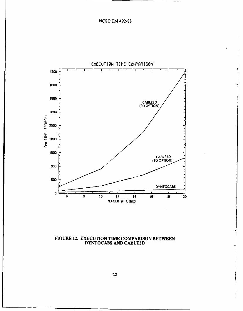
Figure 12 shows the execution time in seconds incurred on a VAX 8650 for each of the runsdescribed above (as well as a 20-link model) as a function of the number of links in the model. Itis clear that the execution time required by DYNTOCABS is well below that required by CABLE3D,especially as the number of links in the model is increased. DYNTOCABS required one-fifth theexecution time that CABLE3D (3D option) required for the 5-link model, and it required one-twentysixth of the execution time that CABLE3D (3D option) required for the 20-link model.

DISCUSSION

A set of algorithms are presented that have been implemented into a computer code calledNCSC - DYNTOCABS. The towed systems may be submerged or partially submerged. They mayhave one or many open branches, but must be towed from a single point. The physical propertiesof the cable may change from one segment of the cable to the next. The cable may be attached toa set of towed spheres or more general towed vehicles with control surfaces. The spheres may belocated anywhere along the cable, but the towed vehicles must be at the ends of the branches.Finally, the program may be used to perform a linear or nonlinear time-domain or a steady-stateanalysis. The linear time-domain analysis computes small perturbations to a steady-state config-uration due to perturbations in the configuration or perturbations in external inputs, such as the towpoint motion and the control surfaces on the towed vehicles. Additional routines may be added toaid in the design of actively controlled towed systems.

The cable is modeled by a series of rigid links connected end-to-end by spherical joints. Themasses of these links and the forces that act upon them are lumped at the joints of the system. Theeffects of fluid drag, buoyancy, weight, and added mass are included. The nonlinear equations ofmotion of the system are numerically generated using procedures presented herein which are similarto those presented in references 1 and 24. Although exhaustive checks have not been made, theresults produced to date using this approach are nearly identical to those found using the approachpresented in references 6 and 15. Finally, for the reasons noted in reference 24, substantial increasesin execution speed are obtained.

Due to its generality, flexibility, and reasonable execution speed, NCSC - DYNTOCABS isexpected to be very useful in the design of large multibranched towed cable systems.

21

NCSC TM 492-88

EXECUTION TIME COMPRRISON

qooo

3500CABLE3D

(3D) OPTION)

3000U,

S2500

S2000

Li

1500CAB LE 3D

(213 OPTION)1000

S00

DYNTOCABS0 A

6 6 to 12 14 16 is 20NUMBER OF LINKS

FIGURE 12. EXECUTION TIM COMPARISON BETWEENDYNTOCABS AND CABLE3D

22

NCSC TM 492-88

REFERENCES

1. Walton, T. S., and Polacheck, H., "Calculation of Transient Motion of Submerged Cables,"Mathematics of Computation, Vol. 14, pp. 27-46, 1960.

2. Strandhagen, A. G., and Thomas, C. F., "Dynamics of Towed Underwater Vehicles," Report219, U.S. Navy Mine Defense Laboratory, Panama City, Florida, 1963.

3. Paul, B., and Soler, A. I., "Cable Dynamics and Optimum Towing Strategies for Submer-sibles," Marine Technical Society Journal, Vol. 6, pp. 34-42, 1972.

4. Leonard, J. W., "Nonlinear Dynamics of Curved Cable Elements," Journal of EngineeringMechanics Division, ASCE, Vol. 99, pp. 616-621, 1973.

5. Webster, R. L., "An Application of the Finite Element Method to the Determination ofNonlinear Static and Dynamic Responses of Underwater Cable Structures," G.E. TechnicalInformation Series Report No. R76EMH2, Syracuse, New York, 1976.

6. Winget, J. M., and Huston, R. L., "Cable Dynamics -A Finite Segment Approach," Computersand Structures, Vol. 6, pp. 475-480, 1976.

7. Leonard, J. W., and Nath, J. H., "Comparison of Finite Element and Lumped ParameterMethods for Oceanic Cables," Engineering Structures, Vol. 3, pp. 153-167, 1981.

8. Sanders, J. V., "A Three-Dimensional Dynamic Analysis of a Towed System," OceanEngineering, Vol. 9, No. 5, pp. 483-499, 1982.

9. Delmer, T. N., Stephens, T. C., and Coe, J. M., "Numerical Simulation of Towed Cables,"Ocean Engineering, Vol. 10, No. 6, pp. 443-457, 1983.

11. Milianzzo, F., Wilkie, M., and Latchman, S. A., "An Efficient Algorithm for Simulating theDynamics of Towed Cable Systems," Ocean Engineering, Vol. 14, No. 6, pp. 513-526, 1987.

12. Choo, Y., and Casarella, M. J., "A Survey of Analytical Methods for Dynamic Simulation ofCable-Body Systems," Journal of Hydronautics, Vol. 7, pp. 137-144, 1973.

13. Huston, R. L., and Kamman, J. W., "A Representation of Fluid Forces in Finite SegmentCable Models," Computers and Structures, Vol. 14, No. 3-4, pp. 281-287, 1981.

14. Huston, R. L., and Kamman, J. W., "Validation of Finite Segment Cable Models," Computersand Structures, Vol. 15, pp 653-660, 1982.

15. Kamman, J. W., and Huston, R. L., "Modeling of Submerged Cable Dynamics," Computersand Structures, Vol. 20, pp. 623-629, 1985.

16. Huston, R. L., Passerello, C. E., and Harlow, M. W., "Dynamics of Multi-Rigid-BodySystems," Journal of Applied Mechanics, Vol. 45, pp. 889-894, 1978.

17. Huston, R. L., and Passereilo, C. E., "On Multi-Rigid-Body System Dynamics," Computerand Structures, Vol. 10, pp. 439-446, 1979.

23

NCSC TM 492-88

18. Salvadori, M. G., and Schwartz, R. L., Differential Equations In Engineering Problems,Prentice-Hall, New York, pp. 401-408, 1954.

19. Woodward, J. H., "Frequencies of a Hanging Chain Support and End Mass," The Journal ofthe Acoustical Society of America, Vol. 49, No. 5 (Part 2), pp. 1675-1677, 1971.

20. Palo, P. A., "Comparisons Between Small-Scale Cable Dynamics Experimental Results andSimulations Using SEADYN and SNAPLG Computer Models," CEL TM No. M-44-79-5,Civil Engineering Laboratory, Port Hueneme, CA, 1979.

21. Huston, R. L., and Kamman, J. W., "User's Manual for UCIN-CABLE - A Three-Dimensional, Finite-Segment Computer Code for Submerged and Partially Submerged CableSystems," Report No. ONR-UC-MIE-050-183-15, University of Cincinnati, Cincinnati, OH,1983.

22. Kamman, J. W., and Huston, R. L., "User's Manual for UCIN-CABLE m - ATwo-Dimensional, Finite-Segment Computer Code for Submerged and Partially SubmergedCable Systems," NCSC CR 105-84, Naval Coastal Systems Center, June 1984, UNCLAS-SIFIED.

23. Guillebeau, C. A., and Ferrer, C. M., "User's Manual for CABLE3D - A Three-Dimensional,Finite-Segment Computer Code for Submerged and Partially Submerged Cable Systems,"NCSC TM 464-87, Naval Coastal Systems Center, June 1988, UNCLASSIFIED.

24. Wilson, H., and Wang, L. C., "Computational Methods for 3D Dynamics of Cables," BERReport N-. 414-58, Bureau of Engineering Research, University of Alabama, University, AL,1987.

25. Gertler, M., and Hagen, G. R., "Standard Equations of Motion for Submarine Simulation,"NSRDC Report 2510, Naval Ship Research and Development Center, Washington, DC, 1967.

26. Kane, T. R., Likins, P. W., and Levinson, D. A., Spacecraft Dynamics, McGraw-HiU, New

York, 1983.

27. Brand, L., Vector and Tensor Analysis, Wiley, New York, 1947.

28. D'Souza, A. F., and Garg, V. K.,AdvancedDynamics -Modeling andAnalysis, Prentice-Hall,Inc., New Jersey, 1984.

24

NCSC TM 492-88

DISTRIBUTION LIST

Commander, Naval Sea Systems Command, Naval Sea SystemsCommand Headquarters, Washington, DC 20362-5101

(Library) 1

Chief of Naval Operations, Navy Department, Washington,DC 20350-2000 2

Commander, David Taylor Research Center, Bethesda,MD 20084-5000

(Library) 3(Code 1548) 4

Commanding Officer, Naval Underwater Systems Center,Newport, RI 02840

(Library) 5

Commanding Officer, Naval Oceans Systems Center,San Diego, CA 92132

(Library) 6

Director, Naval Oceans Systems Center, Hawaii Laboratory,Kailua, Kaneohe, HI 93863

(Library) 7

Commanding Officer, Naval Research Laboratory,Washington, DC 20375

(Library) 8

Commander, Naval Surface Weapons Center, White Oak,Silver Spring, MD 20910

(Library) 9

Commander, Naval Surface Weapons Center, DahlgrenLaboratory, Dahlgren, VA 22448

(Library) 10

Superintendent, Naval Academy, Annapolis, MD 21402-5000(Library) 11

Superintendent, Naval Postgraduate School, Monterey, CA 93943(Library) 12

Chief of Naval Research, 800 North Quincy Street,Arlington, VA 22217-5000

(Library) 13

Commander, Naval Weapons Center, China Lake, CA 93555-6001(Library) 14

Commander, Naval Air Systems Command, Naval Air SystemsCommand Headquarters, Washington, DC 20361-5 101

(Library) 15

NCSC TM 492-88

Commanding Officer, Naval Civil Engineering Laboratory,Port Hueneme, CA 93043

(Library) 16

Commanding Officer, Naval Ocean Research and DevelopmentActivity, NSTL, MS 39529-5004

(Library) 17

Administrator, Defense Technical Information Center,Cameron Station, Alexandria, VA 22304-6145 18-27