overpaid or underpaid? a state-by-state ranking of public...
TRANSCRIPT
1
Overpaid or Underpaid? A State-by-State Ranking of Public-
Employee Compensation
Andrew G. Biggs
Jason Richwine
April 2014
________________________
AEI Economic Policy Working Paper 2014-04
April 24, 2014
2
Overpaid or Underpaid?
A State-by-State Ranking of Public-Employee Compensation
Andrew G. Biggs
Jason Richwine
April 2014
Abstract
This paper ranks all 50 states according to how costly their public-employee
compensation packages are relative to private-sector standards. Each state’s package is
placed into one of five categories: modest penalty, market level, modest premium, large
premium, or very large premium. The results show that national-level analyses obscure
significant differences in compensation from state to state. Connecticut, for example,
pays its state employees 42 percent more than what similar private-sector workers
receive, but Virginia pays its state workers about 6 percent less. State-by-state political
interest in public-sector pay aligns fairly well with our results: In states where public-
sector pay is an active political issue, state government employees appear to be better
compensated than similarly-skilled private sector workers. In states where state
government compensation is at or below market levels, pay for public employees is
generally less controversial.
3 | P a g e
Introduction
Compensation for government employees has become a major policy issue across the nation. As
governments at all levels struggle to balance their budgets, leading to tax increases and reductions in
government services, many citizens have come to believe that government employees receive excessive
compensation, especially in terms of retirement and healthcare benefits.
As the data outlined in this study will demonstrate, in some cases these beliefs are correct.
However, a remarkably large variance exists in the way that different states pay their employees. For a
number of states, public-sector compensation is not a major problem—in fact, some states appear to pay
below-market compensation to their employees. In other states, however, state workers enjoy
compensation that is far above market levels.
The purpose of this report is to document the state-by-state variation in government employee
compensation, ranking all 50 states according to how costly their compensation packages are relative to
what private-sector employers offer to similarly-skilled employees. We track the relative generosity of
wages and benefits, including pensions, health coverage, retiree health care, paid time off, and taxes paid
by employers on their employees’ behalf. We also consider the value of job security and working
conditions. Finally, we discuss some potential reforms to public-sector compensation in states in which
changes may be desirable. The report has two main sections: first, a summary of the results in a readable
format and then a detailed methodological appendix.
The Importance of Getting Public-Sector Pay Right
Most observers hold that a fairly-paid public employee is one who receives salaries, benefits, and
job amenities equal in total value to what he or she would likely receive in a private-sector job. In other
words, states should pay their employees the market value of their skills. If the total compensation
package exceeds that value, then the public employee could be said to be “overpaid.” If it is below that
value, then the employee is “underpaid.”
This standard for setting public-sector compensation tends to result in an efficient provision of
government services and is intuitively fair to public workers. If a state offers below-market compensation
to its workers, the state may have difficulty attracting and retaining the workers it needs. By contrast,
paying above-market compensation to public employees imposes a needless cost on taxpayers.
This standard requires that we do more than simply compare average public-sector salaries to
average salaries outside of government. Such an approach would be as faulty as claiming gender pay
4 | P a g e
discrimination by looking only at raw salary differences between men and women without considering
non-discriminatory factors that might cause male and female pay to differ. Instead, we must look at the
distinctive characteristics of the public-sector workforce--in terms of education, experience, and other
factors--to estimate the salaries these individuals might receive outside of government. In addition, we
must carefully consider the value of employee benefits, since public employees often receive defined
benefit pensions and retiree health plans that are rare in the private sector. Finally, we analyze non-
pecuniary aspects of public employment, with an emphasis on job security.
In general, private-sector employees will receive total compensation – salaries, fringe benefits,
and job amenities – equal to their “marginal product,” an economists’ term indicating the additional dollar
value of the goods and services that the employee produces. While many idiosyncratic reasons can cause
a given employee’s pay to differ from his marginal product, market forces work to keep average pay in
line with productivity. An employer who pays his employees less than what they produce risks losing his
workers to rival companies, which could lure workers away with slightly higher pay while still making a
profit. Likewise, employers who pay employees more than their marginal product risk going out of
business when labor costs exceed sales revenues.
In the public sector, several factors make it less likely that pay and productivity will move in
tandem.1 First, the government does not generally sell the goods and services produced by public
employees, so wage setters in the government lack a clear idea of the dollar value of what employees
produce. Second, while governments have used pay studies to maintain comparability between public-
and private-sector jobs, many occupations are unique to each sector, and the methodology behind such
comparisons has not always been rigorous. Third, public employees can utilize political influence to raise
their wages above market levels, such as through efforts to aid the election of favored officials.
But merely because public pay could in theory differ from private levels does not constitute
evidence that it does differ. That evidence, if it exists, must be drawn from the data. In recent years, many
articles and studies have been written on public-sector pay, including some by the authors of this
analysis.2 However, none have analyzed public-employee compensation on a comprehensive state-by-
state basis. There are important reasons to fill this gap in the literature.
National-level analyses group all public employees together, thereby hiding potentially large
compensation differences that exist from state to state. What matters for policymakers in a given state is
not the nationwide average, but whether their own state is paying its employees appropriately. A state that
pays its employees too much does not compensate for a state that pays its employees too little, even if
5 | P a g e
public employee compensation were “about right” on average. By comparing their own state to other
states around the country, legislators, voters, and public employees may obtain policy-relevant
information.
Our Study
We restrict our analysis to state government workers employed in non-public safety positions.
The sheer number of different pay systems for local government employment make a comprehensive
analysis of local government pay infeasible. Our results regarding state employee pay in a given state
therefore should not be extended to local government employees in that state, as local government salaries
and benefits can differ significantly from those paid by state governments.
We exclude public safety employees because their work conditions, which may include both
threats to life and limb, differ from other government workers and from private-sector employees in
general.3 Public safety employees also generally participate in different pension and retiree health plans,
which would increase the number of pay systems to be analyzed.
Our study begins with comparisons of public and private salaries, then considers the value of the
various fringe benefits received by state government and private-sector workers. We proceed to examine
the relative levels of employment security enjoyed inside and outside of government, along with other
positive or negative job characteristics that might influence pay. We conclude with measures of total
public-employee compensation in the 50 states.
Our results are based solely on applying standard statistical and economic methods to available
data, requiring few subjective judgments about one state relative to another. The numbers themselves tell
the story. But the results confirm intuitive judgments in one important respect: in states in which public-
sector compensation is a significant political issue, the data tend to show that state government employees
receive a premium relative to private-sector workers. In states in which public-sector pay is less
controversial, the data tend to show that state government employees are fairly paid or, at times, even
underpaid.
A picture of the state government workforce
In analyzing public- and private-sector compensation, it is tempting to simply compare average
salaries, and it is not uncommon to see such comparisons in the media. But a simple comparison of
average salaries will be misleading without taking public-private skill differences into account.
6 | P a g e
Table 1 summarizes a number of characteristics of private-sector employees and state government
workers employed in non-public safety occupations. The data in Table 1, and the broader analysis of pay
in this study, are restricted to full-time employees, interpreted as individuals who work at least 50 weeks
per year and at least 35 hours per week.
On average, private-sector workers earn slightly higher average annual wages but also have
somewhat longer work weeks. State government employees are slightly older, slightly more likely to be
married, and significantly more likely to be women. State governments employ a higher fraction of black
employees but a lower fraction of Hispanics and immigrants than the private sector.
Education is an important driver of earnings, and state government employees have higher
average educational attainment than private-sector workers. State government employees are less likely to
be high school dropouts or high school graduates, and more likely to have a college or graduate degree.
Clearly, a simple salary-to-salary comparison leaves too many important workforce differences
unaccounted for. Given these differences, one might be tempted to simply compare pay between public-
and private-sector workers in the same occupations. However, most economists have rejected this
approach. Many public-sector occupations don’t exist in the private sector, making comparisons in those
cases impossible. Moreover, even when comparable occupations do exist, we cannot be sure that either
the job requirements or the skills of the employees who fill those jobs are equal between sectors. (See the
methodological appendix for a more detailed discussion of these issues.)
Wages
Like most other studies conducted by academic economists, we compare public- and private-
sector pay using the “human capital model” of wages, which the Congressional Budget Office (CBO) has
termed “the dominant theory of wage determination in the field of economics.”4 The human capital model
holds that pay is principally driven by the characteristics of the employee, with residuals due to
geographic differences in costs of living and compensating pay differences for occupational
characteristics. Regression analysis compares the pay of full-time state government and private-sector
workers while controlling for differences in education, experience, and other characteristics that predict
earnings. Any difference in earnings after controlling for these characteristics is taken to be driven by the
sector in which the employee works. This statistical method has been used by economists for decades to
examine pay differences attributable to race, gender, educational attainment, union membership, and other

7 | P a g e
factors. We use data from the Census Bureau’s American Community Survey for the years 2009 through
2012.
Our analysis finds that the average state pays salaries around 12 percent below those paid by large
private-sector employers for similarly-skilled workers. This confirms the traditional belief that public
employees receive lower salaries than private-sector workers. However, as Figure 1 shows, this single
national average hides considerable variation from state to state. There is a 23 percentage point gap
between the lowest paying state – New Hampshire, with a public-employee wage penalty of 21 percent –
and the highest-paying state, Connecticut, with a wage premium of 2 percent.
However, salaries are only one component of total employee compensation, which also includes
fringe benefits such as health coverage, pensions, and paid leave. It is not possible to fully evaluate
public-sector compensation without including benefits along with salaries.
Health Coverage for Active Employees
Employer premiums toward health coverage comprise a large and growing share of overall
employee compensation. We gathered the dollar value of employer health contributions from data
compiled by the National Conference of State Legislatures and from other sources. Because health care
costs and the general cost of living vary from state to state, we express the value of employer-sponsored
health coverage as a percentage of employees’ average wages.
In 45 of the 50 states, public-employee health coverage is more valuable relative to wages than
private-sector coverage. (See Figure 2.) The most generous health coverage relative to wages is paid to
Wisconsin state employees, where employer contributions are equal to 32 percent of the average
employee’s wages, despite recent legislation passed in 2011 that increased employee health contributions.
The least generous state employee health benefits are paid in Utah, where employer-provided health
coverage is on average worth 10 percent of wages.
Retirement Programs
We calculate the value of traditional defined benefit (DB) pensions, defined contribution (DC)
plans such as 401(k)s, and Social Security. Together these can be termed “pension compensation,” as they
constitute deferred income paid through retirement plans. We measure pension compensation net of
employee contributions. Because the composition of retirement benefits can differ significantly between
the public and private sectors and between states, Figure 3 combines these three components into a single
measure of total retirement compensation. The most obvious result is that, in every state, the value of

8 | P a g e
retirement compensation for state government employees far outstrips the value for private-sector workers
employed by larger companies. Even the least generous states pay pension compensation equal to over
one-fifth of salaries, and the value of total pension compensation reaches almost half of employee wages
in several cases. This holds true even when we account for the fact that many state government employees
do not participate in Social Security.
Retirement benefits are more generous in the public sector principally due to DB pensions, which
provide significantly higher benefits than the DC plans that most private-sector workers are offered. The
generosity of public DB pensions is obscured, however, by accounting rules that allow public employers
to make low pension contributions on the premise that their investments will earn high returns without
risk. This accounting issue, which is extremely important in analyzing public-sector compensation, is
discussed in depth in the methodological appendix.
Retiree Health Coverage
Most employees of state governments have access to retiree health coverage, which generally
provides primary health insurance from retirement through Medicare eligibility at age 65, and
supplementary health coverage thereafter. These benefits are referred to as OPEBs, meaning Other Post-
Employment Benefits. Most pay studies to date have ignored the value of retiree health coverage, but the
accruing costs of OPEBS to state governments – and the value of such benefits to employees – can be
substantial. A number of states have reduced retiree health coverage in recent years, but these benefits
remain generous compared to the private sector.
Figure 4 shows the value of retiree health coverage for state government employees. These
figures represent the value of future benefits accruing to state employees in the current year (referred to as
the “normal cost” of the benefits plan). Compared to pensions, implicit compensation through OPEBS is
far more variable from one state to another. In certain states, retirees receive nothing more than the right
to buy into the health plan offered to active public employees. In other states, the right to a generous
future retiree health care plan is a major component of current employee compensation. New England in
particular pays particularly generous retiree health coverage: in Connecticut, retiree health benefits are
equivalent to receiving an additional 18 percent of wages every year of the employee’s working life; in
Massachusetts, 18 percent, and in New Hampshire 19 percent.
As discussed in the methodological appendix, data on private-sector retiree health coverage are
sparse. Many private companies are cutting off retiree health coverage for new retirees, and employers
9 | P a g e
that continue to offer coverage are increasing employee premiums and co-payments. Based on reasonable
assumptions regarding these factors, we assume that retiree health coverage for private-sector workers has
an average value of 0.5 percent of wages. However, the typical value of private-sector coverage varies
from state to state.
Total Benefits
Health coverage, retirement income, and retiree health benefits are the three largest sources of
non-salary compensation for state government employees. To calculate total benefits, we also include
other benefits such as paid leave, unemployment insurance premiums, and employer contributions to
Social Security and Medicare. (See the appendix for details on these miscellaneous benefits.)
Figure 5 shows total fringe benefits as a percentage of employee wages. In all cases, state
government employees receive significantly greater benefits than private-sector employees working in
large establishments. Even the least generous state governments – such as Colorado, Minnesota and Iowa,
where average benefits exceed 50 percent of salaries – pay significantly more generous fringe benefits
than even the best-paying states for private sector employees, where benefits for workers in larger firms
top out at 41 percent of pay. In the most generous states, such as California, New Hampshire and New
York, annual benefits including accrual of future pension and health entitlements are nearly as valuable as
wages. For such employee, benefits constitute almost half of total compensation.
Total Wage and Benefit Compensation
Total compensation is measured as the sum of salaries and fringe benefits. Here we do not
include the value of public-sector job security or other job amenities. Total compensation premiums or
penalties are shown in Figure 6. These indicate the percentage difference in total wages and benefits
between non-public safety state government employees and private-sector workers with similar education,
experience, and other characteristics who are employed in large workplaces.
In the average state, state government employees receive a total compensation premium of around
10 percent relative to private-sector employment. However, because the most populous states tend to pay
larger premiums, the average state government employee receives a slightly larger compensation
premium. Nevertheless, substantial state-to-state variation means that national averages are not
particularly meaningful. For instance, pay differentials range from a compensation penalty of 6 percent in
Virginia to a premium of 42 percent in Connecticut.
10 | P a g e
Some states pay large compensation premiums that are difficult to explain as anything other than
“rents” accruing to public employees. (Economic rents are payments in excess of what is needed to secure
the goods or services provided by the recipient.) Public employees and the unions that represent them are
influential players in the political processes of most states. It is not surprising when other powerful
political interests such as corporations receive subsidies or other forms of economic rent. If public
employees are able to secure similar subsidies, they would be paid as above-market wages or benefits.
This appears to be the case in many states.
In other states, however, differences between public and private sector pay are modest. In a
handful of states, public employees receive lower total salaries and benefits than comparable private
sector workers. In these states, variations from pay comparability might be explainable via differences in
non-pecuniary benefits such as job security. Alternately, there may be earnings-related differences
between public and private sector worker characteristics that standard survey data cannot capture, such as
initiative, leadership, and so on.5
One should not overestimate the importance of small differences between states. Salaries are
calculated using survey data, meaning that there is sampling error. In addition, values for paid time off
and legally-required benefits are averages calculated based upon Census regions, which are made up of
several adjoining states. There also may be minor benefits outside of the main BLS categories that we
have been unable to catch. Thus, it may be more useful to place states into different groups based upon
their relative pay. (Table 2.) Within groups, states are listed from lowest- to highest-paid.
Distribution of pay premiums and penalties
The figures discussed above are for the typical state government employee, ignoring the fact that
not every public-sector worker is treated the same. In particular, public-sector wages and salaries are
relatively more generous for low-earning individuals than for highly-educated employees with advanced
degrees. Similarly, the relative generosity of benefits will vary by wage level, because health benefits are
paid on a flat-dollar basis: while each employee receives the same health benefits, these benefits are more
generous relative to wages for low-earning employees. Finally, better-educated state employees may
receive higher DB pension benefits relative to their lifetime earnings and contributions, because such
workers tend to have more rapid earnings growth over the course of their careers. Since DB pensions are
paid based on final earnings, individuals with steeper age-earnings profiles pay lower total lifetime
contributions relative to the benefits they receive.
11 | P a g e
To track these trends, we calculate wage regressions for state employees broken down by
educational attainment. For each educational group, we calculate the value of fringe benefits--accounting
for health benefits paid on a flat-dollar basis as well as benefits, such as pensions, that are proportional to
earnings. We also adjust DB pension benefits for the effects of different rates of earnings growth by
educational category. Figure 7 displays these wage and total compensation premiums and penalties.
State government employees with less than a high school diploma receive salaries roughly on par
with the private sector. But as educational attainment increases, state government salaries fall behind
those paid to similarly educated individuals employed by large private sector businesses. Employees with
bachelor’s, master’s, professional, or doctoral degrees are subject to average salary penalties in the range
of 18 to 34 percent. However, more generous benefits compensate for lower average wages. When
benefits are added, total compensation for less-educated state government employees lies around 20
percent above private sector levels. Total compensation for bachelor’s degree holders is about even with
private sector levels. Professional degree holders such as doctors or lawyers and individuals with doctoral
degrees appear to receive total compensation roughly 18 percent below private-sector levels, although
certain unmeasured factors may compensate. We discuss in the methodological appendix how state
governments could continue to attract and retain professional and doctoral degree holders despite an
apparent compensation penalty.
Employment security and other job characteristics
The human capital model holds that most pay differences between occupations are attributable to
differences in employee skills, such as education and experience, rather than differences in job
characteristics. However, job amenities or dis-amenities also can affect pay. Specifically, jobs with non-
pecuniary benefits can pay lower wages and fringe benefits, while positions with poorer amenities must
pay a compensating wage premium to attract employees.
Perhaps the most important non-pecuniary characteristic of occupations is job security. Public
employees have greater protection against layoffs and terminations for cause than private-sector
employees. This greater job security acts as an insurance policy against unemployment. If state
government employment offers greater job security, then these positions should pay lower overall
compensation than similar private-sector positions. However, the extent of public-sector employment
security and its value as a form of compensation have rarely been examined in depth. We also analyze
other job characteristics that might cause paid compensation to differ between the public and private
sectors.
12 | P a g e
The extent of public sector employment security
Figure 8 shows unemployment rates for three groups of workers: state government employees
(non-public safety); private-sector workers who are similar to state employees with respect to education,
experience, and other characteristics; and all private-sector workers. Unemployment rates for state
employees and all private workers are tabulated from ACS data for the years 2009-2011.6 Unemployment
rates for private-sector workers with characteristics similar to public employees are calculated using a
regression model in which the probability of being unemployed is calculated after controlling for a variety
of characteristics, including being or having been a state government employee.
On average, state government employees had an unemployment rate of 3.9 percent during the
2009-2011 period. This rate is 5.9 percentage points lower than the overall unemployment rate. The two
sets of individuals are not directly comparable due to skill differences. However, even after controlling
for skills, the state government employee unemployment rate was 4.1 percentage points below private-
sector levels.
There is no state in which government employees have unemployment rates equal to or higher
than similar private-sector workers. Nevertheless, the job security advantage varies from state to state. In
Alaska, for instance, public employees have unemployment rates only 0.6 percentage points lower than
those of comparable private-sector workers; in North Carolina, by contrast, the difference is 6.5
percentage points.
State to state variation is driven in large part by differences in unemployment rate for private-
sector employees, which vary more than unemployment rates for state government employees.
Nevertheless, these figures help represent the value of job security for state government workers. Even
assuming public employees in every state had precisely the same degree of job security, the value to
employees of that job security would depend upon the unemployment rate outside of government. Job
security would obviously have greater value in a state with a higher overall unemployment rate.
For reasons discussed in the appendix, it is difficult to quantify the degree to which positions
offering greater job security should pay lower monetary compensation than less secure jobs. However,
one research publication using Canadian data found that, all other things equal, occupations with 1
percentage point lower average unemployment rates have average wages around 2.7 percent lower than
other jobs. Similarly, jobs with higher unemployment rates paid higher wages as compensation.
13 | P a g e
We employ a theoretical model for calculating the job security premium for public employees
that incorporates state-specific data on unemployment rates, the duration of unemployment, the
availability and generosity of unemployment benefits, and other factors. It generates a more conservative
result that a 1 percentage point reduction in the unemployment rate for an occupation is worth about 1.4
percent of compensation. This implies that the effective value of job security for state government
employees ranges from an additional 0.4 to 10.9 percent of wages, with a mean value of 4.5 percent.
(Figure 9.)
Assigning a dollar value to public sector job security remains controversial, so these illustrative
job security figures are not included in the calculations of total compensation premiums or penalties.
Compensation premiums or penalties inclusive of job security are reported in the appendix.
Other job characteristics
We also investigate a number of other factors that have been shown to influence pay. Using the
O*NET database of occupational characteristics compiled by the Department of Labor, we analyze four
categories of negative job characteristics that have been found to generate compensating wage
differentials: conflict, such as with customers or members of the public; physical environment, such as
having a noisy, cold or dangerous workplace; physical demands, such as lifting, stooping, or climbing;
and stressors, such as performing repetitive work or working under time pressure. Each is measured on a
one-to-five scale, with a value of five representing a strong presence of the particular job disamenity.
(Figure 10.)
In two of the four categories – conflict and job stressors – state government and private-sector
occupations are approximately equal. In the remaining two categories, physical environment and physical
demands, private-sector jobs are more unpleasant than state government occupations. If anything, we
would expect that private-sector jobs should be paid a wage premium relative to state jobs to compensate
for these negative job characteristics. If so, then the compensation premium paid to state government
workers in most states may be understated.
Public pay reforms
As noted above, small positive or negative deviations from pay parity are not necessarily a major
concern, given the uncertainties – ranging from sampling error, to the possible exclusion of minor
benefits, to compensating wage differentials for job security and other job amenities – inherent in this
type of analysis. However, in a number of states, compensation premiums are large both in percentage
and dollar terms. These represent significant inefficiencies in public-sector human resource management.
14 | P a g e
Such inefficiencies imply that state governments could reduce compensation costs without endangering
their ability to attract and retain the quality employees they need.
In theory, the savings could come from any part of compensation – wages, health coverage,
pensions, and so on. But it may make sense to focus on aspects of compensation that are most generous
relative to private-sector levels, as these are the areas in which public employees are likely to place the
least value on marginal changes. For instance, if an employee already receives a retirement package of
pensions and health coverage that is several times more generous than his private-sector counterparts,
small increases or decreases in the value of this package are unlikely to cause that employee to quit.
Fitzpatrick (2011) finds, for instance, that some public employees will not purchase additional pension
benefits when given the opportunity to do so on very advantageous terms, even when the option is clearly
explained. From this, Fitzpatrick calculates that “teachers would prefer $2.00 increase in current wages to
a $10 increase in the PDV [present discounted value] of annuitized wealth in their retirement package.”7
In other words, public employees may be so saturated with pension benefits that they are unwilling to
give up even a small portion of their wages to further increase their retirement income. A similar-sized
reduction in government salaries—which are already below private-sector levels on average--could have
more negative effects on governments’ ability to attract and retain employees.
In addition, it may make sense to address public-sector compensation in areas that are least
transparent in terms of cost and value. The accounting standards for public-sector pensions present a
misleadingly low value for these benefits. This lack of transparency confuses budgeting, makes it difficult
to accurately compare public- and private-sector compensation, and may make public employment less
attractive than a comparably sized increase in salaries.
In exchange for more competitive wages, state government employees might be willing to accept
a more modest benefit package, such as shifting from generous defined benefit pensions to defined
contribution plans, raising retirement ages, or accepting higher premiums and co-payments for their
retiree health packages.
As an alternative to reductions in the generosity of DB pensions, certain cities and states have
enacted pension reforms that incorporate greater risk-sharing between employers and employees. Since
risk has a cost, such reforms do reduce both the overall value of pensions to public employees and the
cost of such plans to employers. But they retain many of the attributes of DB plans – such as universal
participation, lower administrative costs, and annuity payments in retirement – that public employees
appear to value.
15 | P a g e
Conclusions
Public-employee compensation is an important and controversial policy issue in states around the
country, but states differ greatly in their approach to it. For that reason, we have produced the first
comprehensive state-by-state comparison of public- and private-sector compensation. We show that state
government employees in most states receive greater total compensation than similarly educated and
experienced private-sector employees who work for large employers. Public-employee wages in nearly all
states fall below those paid in the private sector, but fringe benefits – in particular health and retirement
benefits – are significantly more generous in government than in the private sector. In addition, public
employees in every state have greater job security than they would likely enjoy outside of government.
The compensation premium is not uniform across the nation. Many states pay government
employees at market levels. Others pay huge premiums, and still others fall somewhere in the middle.
Because there are large differences from state to state, broad generalizations and national-level analyses
are not especially useful to the policymakers who must make budgetary decisions for their own states.
This analysis can inform those decisions.
16 | P a g e
Methodological Appendix
In this section we discuss our data and methods in more detail. Much of this material is
necessarily more technical, but we have attempted to present it in as accessible a manner as possible. It is
important for readers to understand how these figures are generated, in particular because alternate
analyses may produce different results. Without understanding the pros and cons of the different
methodologies applied, policymakers and the public are confronted with a “he said, she said” situation
with regard to public-private comparisons, tempting some to simply throw up their hands and give up.
Previous literature
Modern analysis of public-sector pay began with the work of Cornell University economist
Sharon Smith in 1976, who was the first to apply the now-standard human capital model to comparing
salaries for federal government and private-sector employees.8 That analysis, and most others that
followed, concluded that federal government employees receive a salary premium relative to similar
private-sector workers. Following Smith, other economists both expanded on the human capital approach
and adopted alternative methods. Princeton University economist Alan Krueger, who until 2013 served as
the Obama administration’s chief economist, analyzed the number of applications for federal versus
private-sector jobs, concluding that federal jobs on average received 25 percent to 38 percent more
qualified applicants than private-sector positions.9 Dartmouth College economist Stephen Venti used a so-
called “job queues” approach, finding that three to six times as many individuals would be willing to
accept federal employment as there are jobs available.10
Due to this excess demand for federal jobs, Venti
concluded, federal pay could be reduced without impacting the ability to attract qualified employees.
During the 1990s and 2000s, research on public- and private-sector pay was relatively quiet.
Research picked up again beginning around 2010, most likely in response to the economic slowdown that
began in late 2007.
In a 2010 study published by the Center for State and Local Government Excellence, Keith
Bender and John Heywood of the University of Wisconsin-Milwaukee analyzed pay and benefits for state
and local government employees on a national basis.11
Bender and Heywood concluded that state and
local government employees are slightly underpaid compared to similar private-sector workers. However,
their study did not correctly value the defined benefit pensions offered to public employees and failed to
count retiree health benefits. In addition, while Bender and Heywood calculated pay for several individual
states, they did not do so on a 50-state basis.
17 | P a g e
A series of state-specific studies authored by Rutgers University economist Jeffrey Keefe and
published in 2010 and 2011 by the Economic Policy Institute face similar issues. Keefe’s papers, which
generally show public employees to be equally paid or slightly underpaid in terms of total compensation,
do not correctly value public pensions and in most cases do not include retiree health coverage. In
addition, while Keefe’s studies focused on states in which public pay has been controversial, the benefits
data used in Keefe’s studies is specific only to the Census region level, making detailed state-by-state
comparisons impossible.
In 2010, John Schmitt of the Center for Economic and Policy Research analyzed wages for state
and local government employees nationwide, with a particular focus on results by gender.12
However,
because Schmitt did not include fringe benefits, the study does not allow for comparisons of total
compensation.
Beginning in 2010, we have authored a number of studies comparing federal, state, and local
employees with similarly-skilled private workers.13
These studies were the first to analyze public pension
compensation on a fair-value basis and to include retiree health coverage. However, these papers did not
use state-specific values for employer-sponsored health coverage, instead relying upon Census Region-
level data as Keefe did. Moreover, not every state was covered, and the methodology and assumptions
changed as the literature progressed.
In 2011, Alicia Munnell, Jean-Pierre Aubry, Josh Hurwitz, and Laura Quinby published an
analysis of state and local government pay for the Center for State and Local Government Excellence.14
Like our analysis, it valued DB pension compensation on a market basis and included the value of retiree
health coverage. However, it valued DB pensions using a 6.25 percent discount rate, which is
significantly higher than the interest rates that are commonly used in the academic literature. The Munnell
et al. study also reduced the value of retiree health coverage by half as compensation for the possibility
that future benefits may be reduced. We believe that this type of adjustment is inappropriate for a pay
comparison, for reasons discussed below. The Munnell et al. study analyzed all state and local
government employees as a group, concluding that on average they are about fairly compensated.
However, nationwide averages may obscure large differences in compensation that exist from state to
state.
In 2012 the Congressional Budget Office published two studies looking at federal employee
compensation. The CBO’s analysis of federal pay followed our approach to valuing DB pension
compensation at fair market value and also included the value of retiree health coverage.15
The CBO
18 | P a g e
incorporated new methods in terms of analyzing public employee wages.16
Previous studies, including our
own, used the natural log of employee wages as the dependent variable in a wage regression, a technique
that has been utilized for decades and is used in most of the other pay studies discussed here. However,
the CBO noted that, because the distribution of wages is more compressed in the public than the private
sector, this approach can lead to distorted results. The CBO utilized an alternate specification to address
these issues which showed a smaller wage premium for federal employees than the methods used in most
previous studies. The CBO studies concluded that federal employees, on average, receive total
compensation 16 percent above private sector levels.
Also in 2012, two Bureau of Labor Statistics economists, Maury Gittleman and Brooks Pierce,
published an analysis of state and local government pay using a different dataset and techniques.17
Whereas most other studies analyzed human capital in terms of the education and experience of the
employee, Gittleman and Pierce used a BLS dataset that includes an assessment of the skill requirements
of the job position. Gittleman and Pierce concluded that state government employees receive wages
slightly below, and local government employees slightly above, private sector jobs demanding similar
levels of skill. When benefits are included, both state and local government employees receive total
compensation premiums, although Gittleman and Pierce do not value DB pensions on a market basis and
do not include retiree health coverage.
In a series of papers published in 2012 and 2013, William Even of Miami University and David
Macpherson of Trinity University analyzed pay and benefits in specific states, generally finding total
compensation premiums qualitatively similar to those reported here. 18
Even and Macpherson value DB
pension compensation at market value and include the value of retiree health coverage. Even and
MacPherson do not control for differences in firm size, thus producing somewhat higher relative public-
sector wages than in our analyses. However, Even and MacPherson adopt Munnell et al.’s reduction to
retiree health coverage, a step that roughly offsets the effects of omitting a firm size adjustment for
wages.
In this study, we have built on both our previous work and the work of others in an attempt to
apply the most up-to-date methodologies and uniform standards to state government employees in each
state.
19 | P a g e
Wages
The largest component of compensation for most employees is salaries. We compare salaries for
state government, non-public safety employees to the salaries these individuals would likely earn in
private-sector occupations. However, there are several approaches to making such comparisons.
Some studies compare salaries for public-sector occupations to the same occupations in the
private sector. While intuitively reasonable, there are several problems with this approach. First, many
jobs differ between government and the private sector, making direct job-to-job comparisons impossible.
Belman and Heywood show that nearly one-third of public-sector jobs have no clear private-sector
counterparts with which they could be compared.19
Second, even when jobs have the same occupational labels, we cannot be sure that the content of
the job is comparable. In the federal government, for instance, a common problem is “over-grading”– that
is, labeling a position as involving more difficult tasks or greater responsibility than it actually does.20
Third, even when individuals hold the same job, they may bring different levels of skills to the
table. A study of BLS occupational data by Famulari (2002) finds that, “Federal workers have
significantly fewer years of education and experience than private sector workers in the same level of
responsibility in an occupation.”21
If the same pattern held true for state government workers – or if state
employees had greater skills than private-sector workers holding similar jobs – then a job-to-job
comparison will report a pay premium or penalty where none may exist.
Some studies have attempted to address these problems by analyzing the skills required for
public- and private-sector jobs. As discussed above, Gittleman and Pierce use BLS data that rate job skill
requirements based on the General Schedule scale used for setting federal employee salaries.22
If both
sectors are compared using the same criteria, Gittleman and Pierce’s dataset is potentially very useful.
However, state-by-state job ratings are not publicly available.
Like most economists, we rely upon the “human capital model” to analyze wages. The human
capital approach compares salaries after controlling for differences in other individual characteristics –
including education, experience, and other factors – that have been shown to be significant drivers of
salary variation among workers. In additional to numerous studies on the public sector, the human capital
approach has been utilized for studies of pay differences due to race, gender, and union status. The human
capital model is familiar to and accepted by nearly every trained economist.
20 | P a g e
We use data from the American Community Survey, an annual survey of households conducted
by the Census Bureau. We choose the ACS over another popular dataset, the Current Population Survey,
for three reasons: First, the ACS includes more detailed geographic data, which allow us to control for
differences in average wage levels across geographic areas. Without such controls, we might compare
public employees in a high-wage, high cost-of-living area to private workers in a low wage, low-cost area
(or vice versa), thereby generating a phantom pay difference. Taylor (2008) shows that geographic factors
are important in analyzing pay for public school teachers,23
and our own experiments show that detailed
geographic controls can also be important in analyzing state employee pay.
Second, the ACS contains data on the college majors of individuals with undergraduate degrees.24
College majors are correlated with earnings in the workforce due to differences in demand for various
majors, in the skills imparted during college, and in the pre-college abilities of individuals pursuing
different courses of study. Data on college majors provide additional indicators of what state government
employees would likely earn in the private sector. Controlling for college major generally makes public
employees appear less well-paid relative to the private sector, meaning that it either reduces their salary
premium or increases their salary penalty. This indicates that, in addition to having more years of
education than the average private-sector worker, state government employees tend to have college
majors in areas that garner above-average pay in the private sector.
Third, the ACS has a far larger sample size than the CPS. The ACS yearly sample size is roughly
15 times as large as the CPS. Sample sizes in the CPS would be inadequate for analyzing small states.
We assess public employee pay using regression analysis, which examines how differences in a
number of independent variables – such as education, experience, whether the individual is employed in
the public sector, and so on – translate into changes in the dependent variable, in this case annual
earnings. The independent variables cannot perfectly predict salaries for any given individual. The
regression analysis does, however, calculate values for the independent variables that minimize errors in
predicting the value of the dependent variable. Thus, while regression analysis cannot prove that any
single individual is over- or under-paid, it can indicate whether pay differs systematically between the
public and private sectors.
Following standard practice, we regress the natural log of annual wages on controls for years of
education, field of undergraduate study, and potential years of work experience, along with demographic
variables including race, Hispanic ethnicity, gender, marital status, immigrant status, and geographic
location, along with a dummy variable designating whether an individual is a state government employee
21 | P a g e
in a non-public safety position. All individuals in the sample are either state government employees or
private sector workers. We restrict our sample to full-time employees, meaning individuals who work at
least 50 weeks in a year and 35 or more hours per week.
The coefficient assigned to the dummy variable for state government employment represents the
salary premium or penalty paid to state employees after controlling for the other variables present in the
regression. Because salaries are expressed in log form, the coefficient is converted to a percentage.25
This
process is repeated on a state-by-state basis.
Taking the log of wages before running the regression has been standard practice for decades, as
it provides a better fit for the model and allows for easy interpretation of wage difference as percentages.
However, recent research has questioned the use of logs in wage regressions.26
The reason is that private-
sector wages exhibit greater variance (have more high earners and low earners) than state wages. Logs
compress both wage distributions, effectively de-emphasizing some of the highest-paid private-sector
workers but leaving state workers less affected. Taking the log could therefore make private workers
appear less well-compensated (relative to state workers) than they really are.
As mentioned above, the CBO used a more sophisticated regression that does not involve taking
logs.27
Pierce and Gittleman did take logs but employed a post-hoc adjustment to account for the different
error distributions. We do not consider either solution to be ideal. In our own work, we’ve found that non-
logged wages produce an inferior fit, and the results are highly dependent in some states on the type of
regression technique that is chosen. We also found the Pierce and Gittleman adjustment to be an over-
correction in many cases, as it tends to make private-sector wages appear lower than even the non-logged
approach. Nevertheless, the “log problem” in pay comparisons is a serious issue that demands more
attention, and we hope to further address it in future versions of this paper.
More broadly, while the techniques and data we use are widely accepted, continued research on
public-private salary differences is needed. While the ACS and similar datasets provide large sample
sizes, the variables measured may hide heterogeneity between public and private workforces. For
instance, while the ACS does allow us to differentiate workers by college major, it implicitly assumes that
each worker of a given college major attended the same quality college, had the same academic record,
and so on. Similarly, the standard experience variable in a wage regression is in fact a measure of
potential work experience, but cannot distinguish individuals who work continuously from those who
have taken time out of the workforce. These and other issues may be explored using alternate datasets,
22 | P a g e
albeit with other limitations such as smaller sample sizes and the inability to calculate pay differentials on
a state-by-state basis.
Controlling for firm size in the public sector
While the ACS contains important geographic and educational data, it lacks information
regarding the size of the firm for which employees work. Firm size has been shown to influence salaries
independently of employee characteristics such as education and experience. Because state employees
tend to work for larger employers than similarly-qualified private sector workers, a firm size adjustment
will lower relative pay for state workers. Studies such as Keefe (2010), Munnell et al (2011) and our own
prior work have included firm size controls.28
Other recent studies, including Gittleman and Pierce (2012)
and Even and Macpherson (2012), do not control for firm size.29
Firm size controls remain controversial in public-private pay studies because it has not been
established precisely why larger firms pay higher salaries than smaller employers. Moreover, while
economists have suggested many potential reasons for the large-firm premium in the private sector, it is
not clear how well those reasons apply to government.
For instance, it is possible that larger firms pay higher wages because these firms are more
productive, and these productivity advantages are subsequently shared with workers. Even if true,
however, it is unclear whether productivity and workforce size grow together in the public sector. It may
be that smaller local governments, which focus on essential public goods such as police and fire
protection, provide greater benefits relative to resources than larger governments that take on more
marginal tasks. Larger units of government could have a greater ability to pay employees, given
taxpayers’ more limited ability to relocate to lower-tax jurisdictions, but this does not seem an appropriate
reason to control for firm size in public-private pay comparisons.30
Economists also argue that large firms may pay a wage premium to avoid the threat of
unionization. The public sector, however, is already far more heavily unionized than the private sector,
making such a precautionary wage premium unnecessary.
Economists have also suggested that large private firms might be forced to pay employees more
as compensation for certain negative aspects of working for a large organization, such as bureaucracy and
inflexibility. These may be more important factors in government than in the private sector. However, as
we demonstrate in this study, it’s not clear that public-sector jobs have more dis-amenities than private-
sector jobs.
23 | P a g e
Finally, large employers may hire more skilled employees, even after controlling for differences
in education and experience. For instance, a large business with a skilled human resources department
might be better able to identify and recruit employees who are more productive than seemingly
comparable workers in smaller firms. If governments can also utilize their size in this way, this would
justify wages at the level of large private-sector firms.
There is evidence that the firm size premium has been declining, and that these reductions have
been particularly large for less-educated employees.31
We treat the firm size premium as constant across
worker educational attainments, although education-specific firm size salary differentials may be
incorporated into future revisions.
At present it remains common to include a firm size adjustment, and we do so in our figures. We
calculate firm-size controls on a state-by-state basis using data from the CPS, then apply the wage
differential associated with being in a large firm to the salaries received by state government employees.
This adjustment lowers state employees’ relative salaries by an average of around 6 percentage points,
with the smallest firm-size adjustment being 2 percent (Utah) and the largest 12 percent (Vermont). For
researchers who feel that firm-size controls are inappropriate in public-private pay comparisons, the state
firm-size adjustment factors are reported in Table 3.
Grafting a firm size adjustment derived from the CPS onto ACS data may produce erroneous
results if variables included in the ACS regression but not the CPS, such as geographic units and college
majors, correlate with firm size.32
If so, an ad hoc firm size adjustment will lower relative state employee
pay too much. Nevertheless, we believe our basic approach is reasonable.
Benefits
Fringe benefits form a major component of overall compensation, particularly in the public
sector. Moreover, while most state government employees receive a salary penalty, public-sector benefits
are more generous than those outside of government. Thus, without a detailed examination of the relative
generosity of public- and private-sector benefits, we can draw no solid conclusions regarding overall
comparability of public–sector compensation.
Most analyses of public employee pay utilize the Bureau of Labor Statistics Employer Costs for
Employee Compensation (ECEC) dataset, which tracks employer contributions toward a variety of
different fringe benefits.33
The BLS compiles data on benefits for private-sector employers and for state
24 | P a g e
and local governments. These data are collected through the National Compensation Survey. For
simplicity, benefits are expressed as a percentage of worker salaries.
While we use the ECEC data in certain instances, it also has several important limitations. We
rely much less on ECEC data than other researchers, for the following reasons:
First, for defined benefit pensions the ECEC records only the employer’s pension contribution in
a given year, which can differ significantly from the value of benefits accruing to employees in that year.
As discussed later, we instead rely on data from state pension plans, with the discount rate adjusted to
account for the guaranteed nature of public DB pension benefits.
Second, the ECEC does not record the value of retiree health coverage accruing to employees--as
these benefits are generally unfunded, there is no employer contribution to record.34
This, of course, does
not mean that these benefits have no value to employees or no cost to employers. We turn to accounting
reports made by state governments that disclose the value of accruing retiree health benefits.
Third, the ECEC dataset is not available on a state-by-state basis. This is not a disqualifying
weakness for benefits that are smaller and more uniform from state to state, such as paid vacation and
employer contributions to Social Security and Medicare, and we rely on the ECEC in such cases.
Moreover, for private-sector employees, averaging across regions is not terribly problematic, as private-
sector compensation is generally driven by market forces that cross over state lines. For governments,
however, where compensation is set by specific policies, this averaging by region can introduce
inaccuracies in the larger benefit categories. For that reason, for major benefits – health insurance,
pensions, and retiree health coverage – we use state-specific data drawn from outside sources.
In cases in which we utilize ECEC data, we compare public-sector benefits to those paid to
individuals employed in establishments of 100 or more employees. Establishment size refers to the
number of employees at one work site, whereas firm size is the total number of employees working for a
company regardless of location. BLS data indicate around 43 percent of the workforce is employed at
establishments of 100 or more employees. This captures a similar percentage of the workforce as the firm
size controls used in the wage regressions, where the largest firm size is categorized as 1,000 or more
employees. Thus, we are in general comparing public employee salaries and benefits to those paid by
larger private-sector employers.
25 | P a g e
Health coverage
According to the BLS, 99 percent of full-time state and local government employees are offered
employer-sponsored health coverage.35
Coverage is somewhat less prevalent in the private sector,
although the vast majority of full-time employees at larger private-sector firms are offered health
insurance. For instance, 86 percent of full-time private sector employees are offered health coverage, as
are 85 percent of both full- and part-time employees in establishments of 100 or more workers. 36
While
ECEC data do not allow us to calculate the conjunction of these classes, coverage among private-sector
workers who are most analogous to state government employees is doubtless high. The BLS ECEC data
provide the average value of health coverage for all employees, thereby accounting for the small number
of private employees who are not covered.
As noted above, ECEC data are broken down only to the level of Census region, meaning that
state-by-state figures are unavailable. For private-sector workers, this aggregation of states into regions is
probably not of great importance, given that employee benefit costs are driven in large part by broader
economic trends.
However, benefits for government employees can vary widely from state to state. Given the
importance of health coverage in overall employee compensation, for public employees we compile
health benefits on a state-by-state basis. Our principal source is data compiled by the National Conference
of State Legislatures (NCSL).37
These data show monthly employer and employee health premiums for
individual and family coverage in 2012. In certain cases, data for 2012 were not available through the
NCSL. In these cases we used NCSL data from prior years, adjusted upward by the rate of growth of
overall health premiums through 2012. In several other cases, we obtained data directly from state
sources, such as budget documents.
Employee contributions toward health coverage differ in the public and private sectors. On
average, state and local government employees pay 13 percent of their total health care premiums,38
versus 20 percent for private-sector workers in establishments of 100 or more employees.39
Similarly,
around 30 percent of state and local government employees make no contribution toward their health
coverage,40
versus 13 percent for private-sector employees.41
The median state and local government
employee contributes $70 per month toward single coverage and $348 per month toward family
coverage.42
Among private-sector employees, single coverage typically costs $88 monthly and family
coverage $322.43
26 | P a g e
But our approach is to capture the value of employer health care contributions. To the degree
employees contribute out of their own funds this merely reduces their take-home pay, which already is
counted via wages. Thus, we count only the employer contribution as part of employee compensation.
Consistent with private-sector trends, we assume that half of employees choose individual coverage and
half choose family coverage. Employer health contributions are divided by average annual full-time state
employee salaries as reported by the Bureau of the Census to generate employee compensation via health
coverage.
Pensions
Differences in structure between defined benefit (DB) and defined contribution (DC) pensions
complicate the task of comparing the generosity of retirement benefits for public- and private-sector
employees. The fact that they are set up so differently has generated confusion in comparing the levels of
“pension compensation” received from the two plan types. As Belman and Heywood put it in 1993,
“Since one type of plan fixes the costs, but provides an uncertain benefit, and the other type of plan fixes
the benefit but gives employers an uncertain cost, it is very difficult to compare the relative costs and
benefits of the plans. This complicates public/private comparisons because the private sector is more
likely to provide defined contribution plans and the public sector defined benefit.”44
Since that time,
however, more attention has been paid to measuring pension compensation.
Most private-sector employees participate in DC plans. In a DC plan, the benefit received by the
employee at retirement is a function of the employer and employee contributions, as well as interest
earned on those contributions over time. Unlike a DB pension, an employer who sponsors a DC plan has
no obligation to provide a specific benefit at retirement. The employer’s only obligation is to provide a
given contribution to the employee’s account during his working years. For workers with DC plans,
pension compensation is simply the pension contribution made by the employer in a given year.
The vast majority of state government employees participate in traditional DB pension plans, in
which benefits at retirement are a function of the worker’s final salary and years of service. For instance,
an employee might receive a benefit equal to 2 percent of final earnings multiplied by the number of years
he was employed by the government.
For a DB pension participant, pension compensation is equal to the present discounted value of
future pension benefits accrued in a given year, net of employee contributions. For instance, the System
of National Accounts states that “compensation income is… the present value of the claims to benefits
27 | P a g e
earned by active participants through service to the employer.”45
This value of benefits accruing in a
given year is often referred to as the “normal cost” of the pension. It can differ, often significantly, from
the amount that the employer contributes to the plan in a given year.
To calculate DB pension compensation, we first must know the future benefits to which an
employee becomes entitled through an additional year of work. Actuaries employed by public pension
plans perform such calculations based upon projections of earnings, quit rates, longevity, and other
factors.
Second, we must choose an interest rate at which to discount those future benefits to the present.
Importantly, economists choose a discount rate that matches the risk characteristics of the benefit. If the
future benefit is guaranteed, then a low discount rate is used. If the future benefit is risky, meaning that it
may vary or that it may not be paid in full, then a higher discount rate is used. This point is fundamental.
Discounting future benefits using a risk-adjusted interest rate is appropriate regardless of whether
the future benefit is pre-funded (as are DB pensions) or unfunded (as are most retiree health benefits).
Moreover, for pre-funded plans, the discount rate to be used is independent of the investments used to
fund the future benefits. What matters is the risk associated with the benefits, not the risk or return of any
investments used to fund those benefit. This approach is consistent with economic theory, with how assets
and liabilities are valued in private financial markets, and with analyses conducted by a number of
government agencies. (See Sidebar 1 for a summary of expert opinion on this issue.)
Since public employee pension benefits are intended to be guaranteed and in most cases are
protected under state laws or constitutions, a low discount rate should be used to reflect that low risk. In
its analysis of pension compensation for federal government employees, the Congressional Budget Office
used an interest rate of 5 percent, approximately 1 percentage point above the Treasury yield, “because
federal pension obligations are not protected by the constitution.” Since we are analyzing pensions that do
carry legal protections, a lower discount rate is warranted. Academic analyses of state and local pensions,
such as Novy-Marx and Rauh (2011) and Brown and Wilcox (2009), have generally used a discount rate
derived from U.S. Treasury securities.
We choose to discount public pension benefits at 4.3 percent, which is the average yield over the
past decade on 20-year Treasury securities. This is designed to reflect the typical accruals of benefits over
the past decade. This approach is slightly different from the “market valuation” literature on public
pension liabilities, which seeks to value liabilities at a given point in time and thus uses a discount rate
28 | P a g e
specific to that point in time. For perspective, the current yield on 20-year Treasuries is around 3.5
percent.46
Other discount rates may reasonably be chosen. The important thing, as economist Barry
Bosworth of the Brookings Institution stresses, is that the discount rate “should be derived from a fully
taxable bond with risk characteristics (including inflation risk) as close as possible to those of the benefit
liability.”47
Discounting public pension benefits at the assumed interest rate on public pension
investments, usually around 8 percent, is not appropriate because the risk of those investments is much
higher than that of the benefits.
Measuring DB pension compensation becomes confused because some studies conflate the value
of future DB pension compensation with the dollar amounts that public employers contribute to pensions
today.48
This approach is incorrect for two reasons.
First, part of the employer’s DB pension contribution goes toward paying off (or “amortizing”)
unfunded benefit liabilities from prior years. Because this amortization payment is unrelated to benefits
earned in the current year, it should not be counted as part of current employee compensation. Likewise,
in other years states may make no pension contribution, either because they judge the payment
unaffordable or, due to high investment returns in prior years, decided that a payment is not necessary.
But the lack of an employer contribution in a given year does not imply that employees earned no benefits
that year. In fact, benefits continue to be accrued as dictated under the plan’s benefit formula, and the
state’s legal obligation to pay those benefits remains unchanged. It is the benefit formula and the
obligation to pay that determine the value of public pension benefits. The employer contribution made in
a given year is irrelevant to the value of pension benefits accruing to employees in that year. As the
Bureau of Economic Analysis notes, “Contributions aren’t always a good approximation for the value of
benefits accrued through service.”49
Second, as mentioned above, states typically calculate their annual contributions using an interest
rate of around 8 percent. For public employees as a group, this is mathematically identical to the
employer guaranteeing an 8 percent return on both on the employer and employee contributions. This
does not imply that every individual employee receives an implicit return equal to the discount rate;
individual treatment varies, typically based on the employee’s length of service.50
But employees as a
group are guaranteed a return on their and their employers’ pension contributions equal to the assumed
return on pension investments. Since there is no market investment that guarantees 8 percent returns, this
29 | P a g e
constitutes a subsidy that increases the employer’s cost and increases the value of pension benefits to the
employee. As Munnell et al (2012) note:
Contributions to private sector 401(k) plans and public sector defined benefit plans are not
comparable. The public sector contribution guarantees a return of about 8 percent, whereas no
such guarantee exists for 401(k)s. Thus, the public sector contribution under-states public sector
compensation.51
Put simply, a dollar of employer DB pension contributions plus an effective guaranteed return of 8
percent is much more valuable than a dollar of DC pension contributions that does not include such a
guarantee.
We estimate DB pension compensation by recalculating normal costs as reported by public
pensions. We utilize all the underlying assumptions made by pension plans with the exception of the
discount rate, which we set at a level appropriate to the risk of public pensions. The Congressional Budget
Office recently used a similar approach in valuing pension benefits for federal government employees,
and the National Income and Product Accounts published by the federal government now value state and
local government employee pension compensation using a risk-adjusted discount rate.52
Thus, our
approach is consistent with both economic theory and the practice of non-partisan government agencies.
It is important to note that discounting public pension benefits using a government bond interest
rate is not the same as assuming that public pensions will invest only in government bonds. As the
Brookings Institute’s Bosworth puts it, “Discounting with a riskless asset does not imply that the fund
must invest in riskless assets.” It is mathematically straightforward to show that, even if a pension plan
invests in stocks or other high-returning-but-risky assets, the total cost of guaranteeing the payment of a
future liability can be calculated by discounting that liability at the interest rate on a guaranteed
investment such as government bonds.53
Thus, we are not making a statement regarding the investment
practices of public employee pensions.
To calculate pension compensation paid from state government pensions, we must convert
normal costs as published by those plans to a measure using risk-appropriate discount rates. To do so, we
gathered data on over 20 plans from California, Florida, Colorado, Washington, and Rhode Island in
which pensions’ own actuaries have calculated pension costs under different discount rates. The median
result indicates that a 1 percentage point reduction in the discount rate raises the normal cost of a plan by
30 | P a g e
around 36 percent. As a check, we performed our own calculations using workers stylized to be typical of
state government employees, which produced similar results.
The factor to convert a normal cost would equal 1.36(re - rra), where re equals the expected return
on plan assets and rra the risk-adjusted discount rate. For instance, the factor to convert a normal cost
calculated at 8 percent to a 4 percent discount rate would be 1.364, = 3.42. From this risk-adjusted total
normal cost we subtract the value of employee contributions to arrive at net pension compensation. For
instance, a plan with a total normal cost of 10 percent of wages at an 8 percent discount rate would have a
normal cost of 34.2 percent of pay using a 4 percent discount rate. If the employee contributes 5 percent
of pay to the plan, his net pension compensation would be equal to 29.2 percent of wages.
In some states, employees share in the risk of plan financing and thus we must alter the
calculations of pension compensation to account for this.54
Risk-sharing reduces pension costs for
employers but cuts employee compensation by a similar amount.
While the precise calculations differ by plan, these figures clearly imply pension compensation
from public plans that typically far exceeds employer contributions to private-sector DC pensions. That
fact stands in sharp contrast with comments from public pension administrators and government
employee unions that public pension benefits are typically “modest.” It is worth highlighting why this
view is mistaken. These claims often cite the average pension benefit paid by a given plan, which indeed
often appears modest. But these averages include both benefits paid to new retirees who had only a few
years of job tenure and thus very low benefits. It also includes benefits paid to older retirees who accrued
their benefits when wages were significantly lower than they are for current employees.55
If we conduct a
side-by-side comparison of a public employee with a typical DB plan and a private worker with a DC
plan, we find that a private sector worker’s 401(k) contributions would need to be extremely high to
match both the level and the safety of the public employee’s benefits. These contributions closely
correspond to the level of DB pension compensation we report for state government employees.
Sidebar 1: What do experts say about pension accounting rules?
Public employee unions and others sometimes argue that the risk-adjusted discounting of pension
liabilities described in the text is a niche movement supported only by a handful of politically-motivated
academics.56
It is therefore important to emphasize how practically unanimous economists and policy
analysts are in support of it.

31 | P a g e
For instance, Donald Kohn, then-Vice Chairman of the Federal Reserve Board, declared in a
2008 speech on public pensions:
While economists are famous for disagreeing with each other on virtually every other conceivable
issue, when it comes to this one there is no professional disagreement: The only appropriate way
to calculate the present value of a very-low-risk liability is to use a very-low-risk discount rate.57
Similarly, the Fed’s director of research and statistics, David W. Wilcox, testified in 2008 that:
These [public pension benefits] happen to be really simple cash flows to value. They’re free of
credit risk. There’s only one conceptually right answer to how you discount those cash flows.
You use discount rates that are free of credit risk. This is one of those things where it just really is
that simple.58
In a 2009 research paper, two economists from the federal Bureau of Economic Analysis note:
If the assets of a defined benefit plan are insufficient to pay promised benefits, the plan sponsor
must cover the shortfall. This obligation represents an additional source of pension wealth for
participants in an underfunded plan.59
Any measurement of public pension liabilities, and the pension compensation conferred on employees,
must capture the full value of this additional source of pension wealth. Since 2013, the National Income
and Product Accounts, which are the official “books” of the United States economy, have measured DB
pension compensation for public employees using a market-based measure that captures the value of
benefit guarantees to employees.
In early 2012, the Congressional Budget Office issued a report on state and local pensions that
was widely taken as a confirmation of the market valuation approach that we employ.60
Later in 2012, the
CBO issued a report on federal employee compensation that valued pensions using a discount rate chosen
to match the risk of pension benefits, not the interest rate the federal employee pension plan assumes it
will earn on its investments.61
In October 2012, the IGM Forum at the University of Chicago’s Booth School of Business
surveyed 39 professional economists with regard to public pension discount rates. This group of respected
economists represents differing areas of expertise and a wide variety of outlooks on the role of
government. They were asked to express their agreement or disagreement with the following statement:
“By discounting pension liabilities at high interest rates under government accounting standards, many
32 | P a g e
U.S. state and local governments understate their pension liabilities and the costs of providing pensions to
public-sector workers.” Thirty-eight of the 39 economists surveyed agreed, with half agreeing “strongly.”
None of the economists surveyed disagreed.62
In July 2012, Moody’s Investor Services announced that its ratings of state and local government
debt would no longer incorporate pension liabilities measured using high 8 percent discount rates.63
Instead, Moody’s will discount pension liabilities using a much lower bond yield, similar to the approach
we have used here.
33 | P a g e
Additional issues
Data on pensions were gathered either from the Public Plans Database compiled by the Center for
Retirement Research at Boston College64
or directly from actuarial valuations published by the plans
themselves. The key pieces of data are expected return on plan assets and the normal cost of pension
benefits derived from it. Using these inputs, it is possible to convert the normal cost using a risk-adjusted
discount rate.
In most cases, state government employees either do not participate in DC pensions or do not
receive an employer match toward a DC plan. Thus, total pension compensation derives from their DB
plan. Some states do have DC plans for public employees, either as an optional substitute for the DB plan
or as a supplement to it. Given the generosity of DB plans versus the DC option, most employees opt to
remain in the traditional program when given the option.
For supplemental DC plans, employers usually do not make matching contributions. One special
case is Oregon. For most Oregon state employees, the 6 percent mandatory employee contribution to the
DB pension is “picked up” by their employer and deposited into a DC account, and thus is included as
part of pension compensation.
Finally, other states have instituted DC plans for public employees in place of DB pensions, but
in most cases only newly-hired workers are affected. For instance, in Alaska only around 1,500 workers
participated in the state’s DC plan in 2009, making up roughly 6 percent of the total workforce. In such
states, this analysis can be interpreted as applying to the majority of public employees who continue to
participate in the traditional DB pension plan.
For private-sector workers, pension compensation may come both from DC and DB plans. For
DC pensions, we use the average employer contribution as reported in the ECEC dataset for the Census
Region in which the worker resides. DB pension compensation is derived from the same ECEC data, but
must be adjusted to account for the fact that part of the employer’s DB contribution funds amortization of
unfunded liabilities rather than the accrual of new benefits. According to the PBGC, normal costs make
up around 52 percent of total employer DB contributions.65
This figure is relatively low because many
private DB plans have been frozen to new employees or new benefit accruals; in these cases, the entire
employer contribution may go toward paying off benefits earned in prior years.
We do not adjust the normal cost for private-sector DB pensions to the Treasury rate. These plans
already calculate their liabilities using a corporate bond yield, as dictated by federal law. This implicitly
34 | P a g e
assumes that the risk of corporate DB pensions is equivalent to the risk of default on corporate bonds. In
the absence of insurance from the Pension Benefit Guaranty Corporation, this is a good approximation: a
company that is unable to service the explicit debt it has issued would also be likely to default on its
pension obligations.
In practice, PBGC insurance makes corporate pension liabilities safer than corporate bonds,
although not as safe as the legal guarantees applied to public employee pension benefits. The PBGC
honors pension obligations only up to a limit based on the individual’s retirement age, which means that
high-income retirees or those who retire early could have their benefits cut.66
Moreover, PBGC insurance
is financed by additional contributions made by employers; it is not provided simply because employers
discount their obligations of the corporate bond yield. Thus, the normal costs of corporate DB pensions as
calculated under current law appear to be good approximations of pension compensation provided
through these plans. In any case, the value of private-sector DB plans is so small relative to overall
compensation that reasonable adjustments up or down would have little impact on the results of our study.
Retiree health benefits
According to the Government Accounting Standards Board (GASB), retiree health benefits “are a
part of the compensation that employees earn each year, even though these benefits are not received until
after employment has ended.”67
Like a DB pension, a working-age employee who is eligible for retiree
health benefits accrues the right to future health insurance or premium payments to be made by his
employer. And, as with DB pensions, this accrual of future benefits should be counted as part of the
employee’s current compensation.
Health benefits can be extremely valuable for public employees who retire early. For instance, the
California Department of Personnel Administration reports that average annual employer payments begin
at slightly above $9,600 in the first year of retirement, rising to $21,000 in the 10th year and to nearly
$50,000 in the 20th year of retirement. Over the course of retirement, the Department points out, the
typical state employee would receive $493,851 in retiree health coverage.68
As noted above, a number of analyses of public employee compensation omit retiree health care.
But without capturing the value of retiree health coverage, it is impossible to provide a full picture of total
employee compensation. But the value of retiree health coverage varies widely from state to state. A few
state governments offer no coverage whatsoever to their employees. Others allow retirees to buy into the
health plan offered to active employees. For these “access only” plans, states report an implicit subsidy,
35 | P a g e
as older retirees are offered the chance to purchase coverage at the lower rates offered to working-age
individuals. Still other states offer partial or full coverage of health costs in retirement, a benefit that is of
significant value to employees.
Unfortunately, retiree health coverage is not included in the ECEC data set. The reason is that,
since most retiree health coverage is unfunded and financed on a pay-as-you-go basis, there is no
employer contribution for current workers.69
However, it is possible to estimate the value of public retiree health coverage through disclosures
required by GASB. Despite the fact that most retiree health plans are unfunded, GASB reporting rules--
specifically, rules 43 and 45--require that governments publish certain statistics that allow us to calculate
the value of accruing retiree health benefits as a percentage of workers’ salaries. As with pensions, this
value is referred to as the “normal cost” of the plan. As the California Department of Education puts it,
the normal cost “can be thought of as the cost for OPEB being earned by employees in exchange for
[their] services now.”70
Gathering data on OPEBs is not straightforward, as there is no national database of plan statistics
akin to the Public Plan database for pensions. Where possible, we collected retiree health data from
actuarial reports issued by health plans serving state government employees. Sometimes states disclose
normal costs and employee payroll directly; in these cases, compensation through retiree health coverage
equals the normal cost as a percentage of employee payroll. This figure automatically incorporates factors
such as eligibility for retiree health and employee participation in such programs. In a small number of
cases, we rely upon data from Munnell et al (2011).
In other cases, only the dollar value of the plan’s normal cost is published, and we obtain payroll
data from pension actuarial reports, which generally cover the same populations of employees. In still
other cases, governments do not publish the normal cost of benefits. However, governments almost
always publish the Annual Required Contribution (ARC), which is composed of the normal cost plus
amortization costs for past unfunded liabilities, and the total dollar value of the plan’s unfunded liabilities.
Governments are required to publish this figure even if they do not make the contribution or even intend
to pre-fund future retiree health benefits. Given the ARC, the unfunded actuarial accrued liability, the
assumed interest rate, and the general practice that unfunded liabilities are amortized over 30 years, it is
possible to back out the value of the normal cost. We have crosschecked our data against Munnell et al
(2011) and find that it is generally consistent.
36 | P a g e
Most retiree health plans are unfunded. Little or no assets have been set aside and benefits are
financed on a “pay-as-you-go” basis. In valuing these future benefits, discount rates are generally derived
from government borrowing costs or low-risk investments, although as Novy-Marx and Rauh (2013)
note, even these rates are generally above current “riskless” yields. Thus, most OPEB plans don’t have
the fundamental discount rate-based accounting issues that plague public pensions.71
However, OPEB
discount rates do vary from state to state, and this affects the calculated normal costs for such plans. This
seems inappropriate in valuing employee compensation unless these differences in discount rates reflect
different levels of risk to employee benefits, which appears unlikely. Based on sensitivity analysis to
discount rates that is often contained in OPEB actuarial reports, the normal cost of retiree health plans
appears to vary by around 16 percent for each percentage point difference in the discount rate.
In addition, there is a small number of states with pre-funded retiree health plans. Based on
GASB accounting rules, these states discount liabilities and calculate normal costs using the much higher
expected return on investments.72
For purposes of uniformity we adjust the normal costs of all retiree health plans to a constant
discount rate of 4.3 percent, the same rate we apply to pension benefits. As with pensions, plausible
alternate discount rate assumptions are possible. However, our approach is designed to result in
uniformity of measurement from state to state. On average, normal costs for OPEBs increase by around
0.7 percentage points due to this adjustment. In around one-third of states the adjustment reduces normal
costs of OPEBs, as the plan had already assumed a discount rate below 4.3 percent. In the remaining
states the normal cost increased--in most cases only modestly, but with larger increases in the small
number of states that pre-fund OPEBs and assume high returns on investment.73
Retiree health coverage is far less common in the private sector, even among larger employers,
and measuring the cost of plans that do exist in the private sector is a challenge. Data are sparse, and the
landscape is changing rapidly. In addition to changes already under way, the introduction of health
exchanges under the Affordable Care Act may prompt more private employers to drop retiree health
coverage. All these factors make calculating the current value of future retiree health entitlements
uncertain.
In its analysis of federal government employee compensation, the Congressional Budget Office
assumed that one-third of private-sector workers employed by large firms were eligible for retiree health
coverage, that the average annual premium in the private sector was $9,423 in 2009, and that employers
contribute 59 percent of the premium cost. The discounted value of these premiums were attributed to the
37 | P a g e
compensation of current employees, generating an implicit value equal to 2.2 percent of private sector
workers’ wages.74
Using the CBO’s value for private-sector retiree health coverage instead of our own does not
have a significant impact on the overall results of the analysis. Nevertheless, the CBO’s estimate of the
value of private-sector coverage may be high for several reasons.
First, while one third of the largest private firms may offer health benefits to current retirees,
Fronstin and Adams note that “these statistics should not be interpreted as meaning that [similar
percentages] of workers should expect supplemental health coverage.” 75
As of 2003, roughly one quarter
of private firms paying benefits to current retirees do not offer them to new retirees.76
This fraction surely
has risen in the past decade. For instance, an Aon Hewitt survey found that in 2011-2012, 11-12 percent
of large employers tightened eligibility requirements for current employees.77
Similarly, a 2012 Mercer
survey found that 17 percent of large employers who currently offer retiree health coverage will soon
eliminate it for future retirees.78
One cannot simply extrapolate from the share of current retirees receiving
benefits to the share of current workers accruing benefits. Keefe (2011) makes a similar error.79
Second, not every employee at firms that continue to offer health benefits for future retirees will
qualify to receive such benefits. As Fronstin and Adams point out, part-time employees often are not
eligible for retiree health coverage, nor are employees who retire without a required minimum job tenure.
The normal cost figures cited above for public-sector employees factor in the possibility that an employee
will not qualify for benefits at retirement. The CBO analysis for private-sector workers does not appear to
do so.
Third, many private-sector firms offering retiree health coverage do so on an “access only” basis,
meaning that retirees may buy into the health plan offered to employees but must do so using their own
funds. As of 2010, half of firms offering retiree health coverage provided access with no premium
support; 24 percent paid premiums up to a defined dollar limit; and 25 percent had no specified dollar
limit.80
In the public sector, a far greater share of the premium is covered by employers.81
For those reasons, it appears likely that the CBO figure overestimates the value of compensation
received by current private-sector employees through the accrual of rights to future retiree health
coverage.82
For our own analysis, we assume that 25 percent of employees of large firms are offered retiree
health coverage (versus CBO’s assumption of 33 percent, based upon the number of retirees currently

38 | P a g e
receiving benefits); that one-half of that group will be eligible for benefits at retirement (CBO implicitly
assumes 100 percent eligibility); and that their employer will cover 25 percent of premiums (versus the
CBO assumption of 59 percent). Based upon these inputs, we assume an average value for compensation
through retiree health coverage of 0.5 percent of wages, significantly lower than CBO’s number.
That said, we recognize that the availability of retiree health coverage will vary from state to
state. While we assumed 0.5 percent of wages as a nationwide average, we allow this value to vary from
state to state based upon the availability of health coverage to current retirees.83
The costs range from a
low of 0.2 percent of wages (Oregon) to a high of 0.8 percent of wages (Arizona and Indiana).
To be clear, almost nothing rides upon these assumptions in terms of the conclusions to be drawn
from this study. Nevertheless, we believe it is important to treat even small benefits as rigorously as
possible, as a base upon which further research can be built.
Some studies argue that the true value of retiree health coverage to public employees is
significantly lower than the figures used here. Keefe (2011) estimates the value of retiree health benefits
by dividing the cost of benefits paid to current retirees by the wages paid to current employees.84
Using
the example of California, he states that retiree health outlays per worker equal just $821 per year, worth
only 1 percent of employee wages. By contrast, the normal cost of retiree health reported by California in
GASB accounting disclosures is almost 13 percent of wages.
Keefe’s approach has two errors. First, he divides benefits paid to one set of employees by wages
paid to a different set of employees, and thus does not represent the value of the future benefits promised
to current employees. It does not matter, as Keefe contends, that retiree health programs are not pre-
funded. Because the normal cost of retiree health benefits calculated by plan actuaries is discounted, it
reflects the value of those benefits regardless of when they are delivered or paid for.
Second, it appears that Keefe divides annual outlays for the California state retiree health plan by
the number of state and local employees, even though most local employees are covered under separate
retiree health plans. Using figures from the actuarial report for California state employees, annual retiree
health outlays equal $5,567 per covered worker, not the $821 that Keefe claims.85
More importantly,
California retiree health outlays average $10,388 per retiree per year. Assuming an average retirement
age of 60, life expectancy of 83 and annual health cost increases as projected by the plan, a typical
California state retiree would collect over $500,000 in lifetime health benefits. This figure is very similar
to that calculated and publicized by California’s Department of Personnel Administration. These lifetime
39 | P a g e
retiree health benefits are equivalent to receiving at retirement a lump sum cash payment of around
$290,000. This amount far exceeds the 1 percent of pay that Keefe claims, even when accounting for
interest, early deaths, and other factors. The actuarial valuations that we use take these (and many other
factors) into account. They are the best expression of the value to current employees of the future benefits
that are promised to them.
Some studies accept the normal costs of retiree health costs as the proper measure of employee
compensation but suggest that, because retiree health benefits may be lowered in the future, their actuarial
value should be reduced. Munnell et al (2011) reduce the normal costs of retiree health coverage by half
to account for the risk of future benefit reductions, and Even and Mcpherson (2012) follow that practice.
But these adjustments obscure the basic goal of a pay comparison, which is to determine whether
government employers promise compensation to public employees that is different from what is paid to
private-sector workers. In effect, the Munnell adjustment assumes that pay reductions that might take
place in the future have already taken place. In doing so, of course, these methods weaken the policy case
for future benefit reductions because they make public-sector compensation appear more comparable to
private-sector levels. Our approach is to calculate the value of the benefits that have been promised. If
these benefits, combined with other employee compensation, are deemed by policymakers to be
excessive, then reductions might be considered.
Other fringe benefits
Pensions, health coverage, and retiree health benefits are the three largest sources of non-salary
compensation for state government employees. They are also the fringe benefits that vary the most from
state to state. For those two reasons, we gathered data on the above benefits on a state-by-state basis using
accounting disclosures and other data sources. The values of the remaining benefits are smaller and vary
less. These other benefits include life and disability insurance, paid leave, and “legally-required benefits”-
-which include employer taxes toward Social Security, Medicare, unemployment insurance, and worker’s
compensation. For these benefits we rely upon data from the BLS’s ECEC dataset. Because these ECEC-
derived benefits are calculated at the regional level, we do not display results by state so as not to imply a
false level of precision.
Paid leave
Paid leave encompasses sick time, vacation days, paid holidays, and personal leave. On average,
paid leave is almost precisely the same in the private sector as in state government, with values of 11.11
percent and 11.06 percent of wages respectively. There are variations from region to region, with some
40 | P a g e
governments providing more paid leave than private employees and others less. Overall, however,
differences between the public and private sector are quite small relative to other fringe benefits. It is
unusual for the value of state and private paid leave to differ by more than 1 percent of wages.
Legally-Required Benefits and the Treatment of Social Security
Analysis of legally-required benefits must begin with a discussion of Social Security. As with DB
pensions, the value of Social Security to employees is distinct from the contributions made to the program
by employers.
Practically all private-sector employees participate in Social Security, meaning that they and their
employers are required to pay taxes into the program. State government employees in 43 states participate
in Social Security.86
For employees in the remaining states, the employer contribution to Social Security
is entered into our database as zero.
For private-sector and state government employees who do participate in Social Security, we
must account for the fact that Social Security is significantly underfunded. Thus, part of the taxes paid
into the system are effectively payments to address the program’s unfunded liabilities – akin to the
amortization payments to public DB pensions, which we exclude from our analysis – not “contributions”
or “normal costs” that generate matching benefits in the future.
Because Social Security is financed on a “pay-as-you-go” basis rather than being “fully funded,”
the program’s actuaries don’t calculate normal costs as public pension actuaries do. Moreover, unlike
public DB pensions, Social Security is a progressive system. As a result, the de facto normal cost as a
percentage of wages will differ based on the earnings level of the participant.
However, it is possible to estimate normal costs for Social Security participants. Social Security’s
actuaries publish “money’s worth ratios,” which represent the ratio of lifetime benefits received to
lifetime taxes paid, both in present value terms. These ratios are calculated for different worker types
retiring in different years.87
This ratio represents the share of the 12.4 percent Social Security payroll tax
that can be considered the normal cost of the system – meaning the portion of payroll taxes the participant
will receive back in full – with the remainder being a “pure tax” devoted to addressing the program’s
unfunded liabilities.
The SSA figures show that for a two-earner couple born in 1964 with earnings equal to 160
percent of the national average – a decent approximation of the typical state government employee –
41 | P a g e
Social Security will pay total lifetime benefits equal to 69 percent of the taxes paid into the program.88
Multiplied by the 12.4 percent payroll tax generates a normal cost of 8.6 percent of wages.
But workers themselves contribute 6.2 percent of their pay to Social Security. To be consistent
with our previous treatment of DB pensions, the employee contribution is subtracted from the gross
normal cost to find the net component that adds to worker’s compensation. This figure – which again is
specific to the age and earnings level of the typical state government employee – is 2.4 percent of wages.
This amount is entered into our database as the net compensation employees receive via participation in
Social Security.
This approach may appear confusing at first. Employers do in fact contribute 6.2 percent of their
workers’ pay into Social Security, so why not include the full amount as part of their compensation? The
reason, as discussed above, is that participants in Social Security lose, on average, around 3.8 percent of
their lifetime wages to the system. That is, they pay this amount in but receive nothing in return for it.
Those payments are, in effect, a “tax.” Workers who don’t participate in Social Security, by contrast, are
exempt from that implicit tax. A comparison of pay that includes both participants and non-participants in
Social Security must account for that difference.
As with our treatment of private-sector retiree health coverage, very little rides on these
assumptions regarding Social Security. The overall results would be changed only slightly by attributing
to employees the full employer contribution to the program rather than the net value that employees
actually receive. In the vast majority of states, where both public- and private-sector workers take part in
Social Security, the effect is zero. But our goal is to be as rigorous as possible in analyzing all forms of
worker compensation, both large and small.
Other legally-required benefits
Other legally required benefits, such as Medicare, unemployment insurance, and worker’s
compensation, are calculated in terms of the level of employer contributions. In general, legally-required
benefits are more generous in the private sector than in state government, at 11.2 percent and 8.8 percent
of wages, respectively. Part of this is due to non-participation in Social Security by some state employees,
but private-sector contributions to Medicare, unemployment, and workers compensation also are
somewhat higher than in state government. For Medicare, this may be due to the uncapped payroll tax,
which is more likely to affect private-sector workers, as very high wages are more common in private
jobs. Employer contributions for unemployment insurance and worker’s compensation are experience-
42 | P a g e
rated, and thus higher contributions would at least in part be due to the higher risk of unemployment or
injury in these positions.
Total Paid Compensation
Total paid compensation is the sum of salaries and benefits. We derive the total compensation
premium or penalty by multiplying wages by (1 + benefits as a percentage of wages), then re-running the
original regression.89
In both the public and private sectors there may be minor benefits that do not fit into the standard
categories measured by the BLS ECEC survey. Moreover, as detailed below, in a competitive labor
market job amenities and dis-amenities can influence the pay and benefits that a position must provide.
Nevertheless, the total compensation figures illustrated in Figure 6 (above) represent, in our view, a
reasonable measure of the relative pay of state government workers.
These figures confirm much of what ordinary Americans already believe about public-sector
compensation, but they also contain some surprises. At a general level, they confirm that while state
government employees may receive less generous average salaries than similar private sector workers, the
more generous benefits package paid in government – in particular, retirement benefits – is sufficient to
make state employment, on average at least, attractive relative to private-sector jobs.
The data also confirm that many of the states in which public-sector pay is controversial do
indeed appear to “overpay” state government workers relative to their private-sector counterparts. No one
would be surprised to see significant compensation premiums in California, New Jersey, or Illinois.
Others, such as Pennsylvania and New York, have traditionally had strong public employee unions who
are powerful political players.
Similarly, compensation is most comparable to private-sector levels in some of the states known
for fiscal restraint. Indiana, for instance, never had strong public employee unions, and former Gov. Mitch
Daniels recently reformed employee health plans. Likewise, Virginia is perceived as a business-friendly
state and does not allow collective bargaining for public employees.
However, there are some surprises. One would not expect that traditionally liberal states such as
Washington and Minnesota would pay state government employees below private-sector levels,
Integrating the value of job security would increase these states’ total compensation packages somewhat,
but even then they would not come close to the premiums in some of the higher-paying states.
43 | P a g e
Likewise, one would not necessarily expect states such as Wyoming or New Mexico to have
among the largest premiums, yet that is what the data indicate. Wyoming pays a total compensation
premium of 21 percent over private-sector levels, while New Mexico pays a premium of 20 percent.
While the principal comparison is of public employees in a given state to similarly-skilled
private-sector workers in that state, our approach implicitly allows states to be compared to each other.
Our results indicate that some state governments compensate their employees significantly more
generously than others. Roughly speaking, the best-paid state (Connecticut) pays its employees
approximately $1.50 in total wages and benefits for each dollar that the lowest-paid state (Virginia) pays.
It is possible to crosscheck these results against more broad-based measures that would intuitively
point toward public-sector pay differentials. Ruger and Sorens (2013) calculate an index of economic and
personal freedoms by state.90
Here we restrict our analysis to economic freedoms, which are compared to
the total compensation premium or penalty calculated for each state. (Figure 11.) The trend indicates that
states with lower economic freedom scores tend to have higher state employee compensation relative to
similarly-skilled private sector employees in that state. The R-squared value is 0.27.
Similarly, Keating (2013) calculates a state index of policy factors relevant to the small business
climate.91
States with a more business-friendly environment appear to pay state government employees a
lower compensation premium (Figure 12). The measured R-squared value is 0.11.
Likewise, when our measured compensation differentials are expressed in rank form, they are
correlated with rankings of state teacher union strength in Winkler, Scull and Zeehandelaar (2012).92
None of these measures are perfect checks, yet they may serve as proxies for some underlying factor
affecting the generosity of public employee compensation.
Compensation at different pay levels
In addition to understanding relative compensation for the average state government employee,
readers may be interested in how relative compensation varies at different pay levels within government.
Generally, this is done by calculating relative compensation for employees with different levels of
educational attainment, which is a strong predictor of earnings. While seemingly straightforward, that
analysis must take into account three major factors.
First, and most basically, the wage penalty or premium that a state government pays is not
uniform throughout the distribution of workers employed by the government. It is generally believed that,
44 | P a g e
due to the relative compression of wages paid in government, public employment is relatively more
favorable to lower-skilled employees and less favorable to high-skill workers.
Second, the value of fringe benefits differs between high and low earners. Some fringe benefits,
such as health coverage, have essentially the same dollar value for all employees. Others, such as
pensions or paid time off, have a value that is proportional to the individual employee’s wages. Fixed-
dollar benefits will favor low earners and earnings-related benefits will favor high earners.
Third, the rate at which an individual’s earnings grow through his career affects the value of
pension compensation from a DB plan. The benefits an individual receive from a DB plan throughout his
retirement are based upon his final earnings. The worker’s contributions, by contrast, are a function of
earnings over the worker’s full career. Individuals with rapid earnings growth – so-called “high flyers,”
who are predominantly better-educated employees – have low average lifetime earnings relative to their
final earnings, and thus pay lower lifetime pension contributions relative to the benefits they receive.
Koedel, Ni, and Podgursky (2013) note that school administrators have more rapid salary growth than
classroom teachers. As a result, administrators receive higher retirement benefits relative to their lifetime
salaries and contributions. For instance, relative to a career teacher, a school principal makes 14 percent
higher lifetime contributions but receives 37 percent greater lifetime benefits. Similarly, a school
superintendent makes 53 percent greater career contributions than a teacher but receives 89 percent higher
total benefits.93
Young (2012) illustrates this same point with reference to the Canadian public sector.94
Analysis of the distribution of relative state government compensation follows three steps. First,
we calculate wage penalties or premiums for state government workers of different educational
attainments. Next, we estimate annual earnings growth for state government employees of different
educational attainments, and use this information to calculate education-specific pension compensation.
Third, based on relative levels of fixed- and earnings-related benefits, we calculate total compensation by
educational attainment.
Table 4 shows wage premiums or penalties for state government employees by educational
attainment. These are calculated using regression analysis controlling for the same factors as in the state-
level wage regressions, but are calculated at a national level. Thus, these figures and the conclusions
drawn from them should be treated as national averages only, bearing in mind the variation in overall
compensation levels we have shown to exist from state to state. After adjusting for firm size effects, all
educational groups appear to receive salary penalties in state government employment, although the size
45 | P a g e
of such penalties differ markedly. State employees with only a high school diploma receive salaries 3
percent below private sector levels, with this salary penalty rising to
Individuals with a high school diploma or less receive salaries that are very close to those paid in
the private sector. All other educational attainments, however, appear to receive lower average salaries in
state government than in the private sector, with the largest salary penalty of 37 percent received by state
government employees with professional degrees. (Figure 7.) The major differences between our analysis
and others is the inclusion of tighter geographic controls and, for college-educated individuals, a control
variable for the subject the individual studied as an undergraduate.
Next, we divide public-sector fringe benefits into two types: flat-dollar benefits and earnings-
related benefits. On average, state employees receive earnings-related benefits equal to 51 percent of their
salaries and flat-dollar benefits equal to 24 percent of their salaries. For any given state employee,
however, benefits are equal to 51 percent of his own salary and 24 percent of the average salary for state
workers, which we calculate as $53,341. In dollar terms these flat-dollar benefits are worth $12,802 on
average, which ranges from 43 percent of salary for state workers with less than a high school diploma to
13 percent of salary for state employees with a professional degree.
We then subdivide earnings-based benefits into pensions and other benefits. Pension
compensation is on average worth 29 percent of salaries and other earnings-based benefits are valued at
22 percent of salaries. As noted above, however, pensions will be more valuable to individuals with rapid
earnings growth, who are generally “high flyers” with greater educational attainments. To estimate the
effects of earnings growth on pension compensation, we begin by calculating average rates of earnings
growth for state employees with different levels of education. Using ACS data, earnings are tabulated by
education for state workers aged 22 to 25 in 1980 and for employees aged 52 to 55 in 2010. While a
rough method, this approach shows that earnings growth is higher for better-educated state employees.
High school dropouts, high school graduates and individuals with some college education have the
slowest rates of annual earnings growth, at approximately 5 percent, while state employees with
professional degrees have the most rapid, at 8 percent.
Using these rates of earnings growth, we build a simple model to estimate the relationship
between the present value of lifetime earnings – and lifetime pension contributions – to final earnings.
For simplicity, each educational category is assumed to have the same final earnings and the same years
of employment, and thus the same pension benefit. Each educational category also is assumed to collect
benefits for the same period of 25 years. But due to different rates of earnings growth prior to retirement,
46 | P a g e
better-educated public employees will pay smaller contributions over their lifetimes relative to the DB
pension benefits they will receive. The relative contributions of each educational category are compared
to those of a stylized average workers whose wages grow by 6.1 percent annually. This ratio is multiplied
by the overall average contribution rate of 6.8 percent of wages. This adjusted contribution rate is then
subtracted from gross pension compensation – that is, net pension compensation of 28.9 percent of wages
plus the average contribution rate of 6.8 percent – to produce adjusted net pension compensation by
educational attainment.
As expected, lower educational categories of state employees receive somewhat lower pension
compensation while more-educated state workers receive above-average pension compensation. For
instance, high school graduates receive pension compensation equal to 27.6 percent of wages while state
employees with professional degrees receive pension compensation of 30.8 percent of wages.
These adjusted pension compensation figures are incorporated into calculations of overall
compensation, where for simplicity total compensation is taken as wages * (1 + benefit ratio). The results
show that the least-educated state employees receive sizable compensation premiums versus similar
private-sector workers, while more-educated state workers receive modest to significant compensation
penalties. Individuals with less than a high school education receive a total compensation premium of 22
percent; high school graduates receive a compensation premium of 19 percent; individuals with some
college receive a premium of 13 percent; college graduates receive a premium of 2 percent; master’s
degree holders a penalty of 3 percent; professional degree holders a penalty of 17 percent; and PhDs a
penalty of 18 percent.
These calculations generate several results. First, as expected, total compensation is more
favorable to state government employees than wage income alone, due to relatively more generous
benefits paid in the public sector. Second, while compensation penalties remain for better-educated state
government employees, the largest compensation penalties are not for professional degree holders (such
as doctors and lawyers) but for individuals with doctoral degrees. While both professional and doctoral
degree holders appear to receive large wage penalties, the higher rate of wage growth for professional
degree holders grants them more favorable DB pension compensation.
Nevertheless, a significant total compensation penalty remains for both professional and doctoral
degree holders. It is worth considering how government may continue to attract better-educated
employees despite a seeming compensation penalty.
47 | P a g e
One possibility is that, despite our efforts to increase the precision of data used in public-private
pay comparisons, systematic but undetected differences remain between the two groups of employees.
The inclusion of undergraduate degree fields reduces measured salary penalties for state government
employees with professional and doctoral degrees by several percentage points. However, the ACS data
do not allow us to control for the possibility that public service might attract individuals who obtained
their degrees from less-prestigious universities or who performed less well in school. Some research has
been conducted in this area using the National Longitudinal Survey of Youth. Black and Smith (2006)
match NLSY data to common measures of college quality and competitiveness, finding that attending a
higher quality college correlates with higher wages even after controlling for individual differences.95
Gittleman and Pierce (2011) use an alternate approach to estimating public-private wage and
compensation differentials, in which they compare pay for public and private jobs with similar skill
requirements. Despite the fact that Gittleman and Pierce do not include retiree health benefits and do not
value DB pensions on a market basis, they find that the vast majority of state government employees
receive higher total compensation than private sector employees working in jobs with similar skill
requirements. Even at the 90th percentile, private sector workers receive total compensation 5.5 percent
below state government employees. (At the median private compensation is 9.3 percent lower and at the
10th percentile it is 13.2 percent lower). These results, in combination with our own, could indicate that
state government employees have better educational credentials than private-sector workers but work in
jobs whose skill demands exceed private levels by a smaller degree.
It also is worth considering how state government can attract and retain employees even assuming
that a compensation penalty exists. One answer is greater job security, the value of which we attempt to
quantity in a later section. The inclusion of job security alone would not close the compensation gap for
highly-educated state employees, though it is possible that highly-educated individuals seeking out public
employment are particularly risk-averse.
In addition, a number of occupation-specific factors may come into play. For instance, private
physicians generally must pay their own malpractice insurance, which can be very expensive depending
on the doctor’s specialty and state of residence. Doctors employed by the government, by contrast,
generally are protected by government indemnity rules and need not carry separate malpractice insurance.
For context, in the year 2000, the most recent year for which survey data were available, malpractice
insurance premiums equaled 8 percent of self-employed physician’s net income.96
Similarly, Dillon
(2013) shows that occupations with high earnings risk pay higher average salaries as compensation.
48 | P a g e
Dillon shows that lawyers have among the highest earnings risk of professional occupations. Lawyers in
the public sector may be willing to accept reduced average salaries in order to lower the volatility of their
annual earnings.
While more difficult to quantify, government employment might also provide better quality of
life, in terms of overtime work, stress, or other factors. We document these differences in later sections on
an occupation-specific basis, but cannot determine if within specific occupations state government
provides more attractive working conditions than the private sector.
The value of job security
Data from the American Community Survey indicate that state government employees have an
unemployment rate roughly 4 percentage points lower than private-sector workers with similar education,
experience, and other earnings-related attributes. Public employees in every state appear to have
significantly greater job security than their private sector counterparts, though this advantage differs from
state to state.
Some have argued that public-sector employees may not enjoy greater employment security than
similar private-sector workers. For instance, Munnell et al. (2011) point out that employment levels for
public employees have risen and fallen roughly in parallel to that of private-sector workers.97
But this
does not imply that job security is similar between the two sectors. For instance, if private sector
unemployment rises from 6 to 8 percent while public sector unemployment rises from 2 to 4 percent,
public employees nevertheless continue to have greater job security than private-sector workers.
Others have pointed to the decline in state and local government employment over the past
several years as evidence that public employees lack job security.98
However, data from the Bureau of
Labor Statistics Job Openings and Labor Turnover Survey indicate that, while there have been layoffs in
the public sector, layoffs have not been the main cause of reduced state and local government
employment. For instance, the state and local government layoff rate rose from 5.6 percent of the
workforce in 2001-2008 to 6.4 percent in 2009-2012, a 0.8 percentage point difference.99
However, the
hiring rate for new employees fell by more than three times that amount, from 17.7 to 14.9 percent. While
there are exceptions, reductions in public-sector employment appear to be predominantly attributable to
attrition, not involuntary job losses.
We have not argued that public employees have a job guarantee; we have shown, however, that
state government employees have a far lower chance of becoming unemployed than private-sector
49 | P a g e
workers with similar qualifications. And this extra job security has a value. Labor economics holds that
non-pecuniary differences between occupations, such as job security and work conditions, will be
reflected in wages and other forms of compensation. To recruit employees to jobs with unattractive or
unpleasant attributes – such as a lack of job security – employers must pay a compensating wage
premium. Likewise, employees will accept lower wages or benefits if the other attributes of their job are
particularly attractive. 100
Job security is not simply one among many non-pecuniary job characteristics. Human resource
surveys show that job security is ranked alongside salary and benefits as the most important attributes of a
position. For instance, the Society for Human Resource Management’s 2010 Employee Job Satisfaction
Survey found that job stability was judged even more important than either benefits or salaries among
workers surveyed. 101
Other human resources studies have found job stability ranked equally with salaries
and benefits, with other job amenities trailing significantly behind.102
Academic research also finds that
job security ranks alongside pay and benefits and well ahead of other job attributes.103
Differences in job security between public and private occupations mean that a simple
comparison of wages and benefits will not fully account for the value of the respective compensation
packages. Such simple comparisons are akin to comparing the returns on stocks and bonds without
considering differences in their risk. Like a bond, a low-risk job may offer a lower expected payout; like a
stock, a high-risk job must offer more.
The wage differential paid to compensate for unemployment risk should be greater than the
expected value of income lost to unemployment, for several reasons. First, unemployment is most likely
to occur at times when the economy is depressed, meaning that the individual loses income when the
availability of other income sources is low. Second, unemployment is disruptive even if the worker
quickly finds a new job. He must conduct a job search, attend job interviews, alter daily work schedules,
and possibly lose personal and professional relationships established in his prior job. A spell of
unemployment is not the same as period of unpaid vacation. Survey data indicate that the unemployed
have significant feelings of anxiety, stress, and other negative emotions, particularly as the duration of
unemployment continues.104
While there is little disagreement that compensating wage differentials exist, the academic
literature notes the difficulty in discerning such effects from the data. The principal reason is that the
variables offered in most datasets – such as years of education or experience – are “broad buckets” that
allow for variation in human capital among seemingly similar individuals. For instance, the experience
50 | P a g e
variable used in most wage regressions reflects only potential experience – the maximum years the
individual could have worked – but does not track actual years in the workforce. Likewise, the education
variable cannot distinguish the average college graduate from a person who earned a high GPA at a
highly-selective school.
As a result, workers who appear similar may have different levels of productivity. All workers,
regardless of productivity, will balance monetary compensation against job amenities, but more
productive workers will tend to get more of both – that is, both higher pay and better amenities. Less
productive workers, by contrast, will receive less pay and fewer non-pecuniary amenities. Hwang et al
(1992) show that these unobserved productivity differences can cause researchers to understate true
compensating wage differentials or even find the wrong sign—meaning, for instance, that jobs with less
security would deceptively appear to pay lower wages. Analysis based on standard data sources and
approaches is “likely to severely underestimate workers’ willingness to pay for job attributes.”105
Some
studies have argued that the difficulty in isolating job security-related wage differences in standard
datasets means that they are of little importance.106
However, as the research cited above explains, one
would not expect to easily isolate compensating wage differences in datasets such as the ACS or CPS.
Researchers have adopted two approaches to addressing these problems. One approach is to use
longitudinal datasets that follow individuals’ earnings volatility over time, rather than comparing earnings
differences among individuals at a single point in time. Because the same person is being analyzed, the
effect of unobserved productivity differences is minimized. Feinberg (1981) used the Panel Study of
Income Dynamics to show that “a significant part of average hourly earnings represents compensation for
earnings-risk.”107
For the average earner in Feinberg’s analysis, roughly 16 percent of hourly earnings
were compensation for volatility of earnings from year to year. Dillon (2012) also used the PSID, finding
that compensation for earnings risk accounts for 17 percent of differences in overall pay between
occupations.108
For instance, she found that employees in financial occupations, which have both high
average earnings and high earnings risk, would be willing to give up 20 percent of their earnings in order
to avoid all earnings risk. Cubas and Silas (2012), using the Survey of Income and Program Participation,
also find a correlation between earnings risk and salary levels between occupations.109
Other researchers have maintained the use of cross-sectional analysis, but narrow the range of
unobserved productivity differences by adding additional information to the standard wage regression.
Kumar and Coates (1982) combined Canadian household survey data on personal characteristics such as
education and experience with employer survey data on the skill requirements of different jobs. While
51 | P a g e
neither the household survey data nor the establishment data alone indicate a compensating wage
differential for the risk of unemployment, Kumar and Coates use the combined dataset to show that a 1
percentage point increase in the unemployment rate for an occupation increases average wages by around
2.7 percent.110
It is difficult to apply the results of the Feinberg and Dillon longitudinal analyses to the cross-
sectional data in the ACS or CPS. However, based on the Kumar-Coates figures, the effective value of job
security for state government employees would range from an additional 2 to 18 percent of wages, based
on state-by-state differences in public and private sector unemployment rates, with a mean value of 11
percent.
Estimating the value of job security for state government employees
As discussed above, data quality issues make it difficult to discern the values of compensating
wage differentials for the risk of unemployment. For that reason, we turn to a simple expected utility
model.
To illustrate the underlying logic, consider a simple game involving the flip of a coin. If the coin
comes up heads, you receive $100; if it comes up tails, you receive nothing. Thus, you have an expected
gain of $50, but no guarantee of anything. You are then offered a second option: receive a guaranteed
cash payment in lieu of the coin flip. The question is, what is the lowest guaranteed payment you would
accept rather than take the 50-50 chance of winning $100? A person who was indifferent to risk would
demand $50, the expected value of the bet. But most individuals are risk-averse, meaning that they will
accept a lower certain amount over a higher amount that comes with risk. The lower amount is referred to
as a “certainty equivalent” value. And the more risk averse an individual is, the lower the certainty
equivalent value he or she will accept. Some might demand $40, while others might willingly accept only
$25.
Employment risk presents choices very similar to the simple game above. Some jobs have a great
deal of employment risk, with a significant chance of being laid off due to the business cycle or poor
performance. Other jobs have much greater job security. The question is, how much of a wage increase
would employees demand to accept a job where employment risk is greater? Likewise, how much less
would they accept to enjoy greater job security? Quantifying this compensating wage differential is more
complex than in the coin flip game, but the underlying logic is the same.
52 | P a g e
To begin, we define a term called the Total Security Wage. For a given job, the Total Security
Wage is the salary that workers would accept assuming there was no risk of unemployment. Obviously,
the Total Security Wage will be lower than the actual wage, since all real jobs – including those in the
public sector – carry some chance of dismissal. But how do we calculate this Total Security Wage? We
begin with a plain-English discussion, then examine some of the numerical assumptions and calculations
in greater detail.
A worker in a job with employment risk earns a given level of salary and benefits while on the
job. Assuming he is not fired or laid off, he enjoys some level of well-being or “utility” from his
compensation. This well-being can be quantified through a utility function that is commonly used by
economists (and is explained in greater detail below). However, if that employee is fired or laid off, he
goes through a period of unemployment in which his income is reduced and the utility he enjoys is lower.
The expected utility he derives from the job is the weighted average of the two outcomes, reflecting both
the income received while working and the risk of lost income through unemployment.
Using the same utility function, we can convert that expected utility back into a single dollar
amount, which represents the Total Security Wage. This dollar amount, like the certainty equivalent value
in the coin flip gain, will be less than the expected pay for the job. The Total Security Wage represents the
lower salary the employee would agree to if his employment risk were reduced to zero. The pay
difference between the job with employment risk and the Total Security Wage represents the
compensating differential for job security. By definition, workers would be roughly indifferent between
the lower-paid job with greater employment security and the higher-paid job with less employment
security.
In practice, calculating the job security premium is more involved because neither private- nor
public-sector jobs have perfect job security. In both cases there is the chance of dismissal, but state
government employees have a significantly lower chance of becoming unemployed. To account for this,
we perform the calculation detailed above twice, once for private-sector jobs and once for public-sector
ones. Assuming equal pay in each job, the Total Security Wage will be lower for private-sector workers
because their jobs carry greater employment risk. Put another way, a greater share of the private-sector
wage is compensation for employment risk. Dividing the Total Security Wage for state employees by that
for private-sector workers and subtracting one gives us the percentage job security premium for public-
relative to private-sector positions.
53 | P a g e
The above paragraphs explain the underlying logic of calculating the job security premium, but
calculating the figures requires a number of assumptions:
Utility: we use an isoelastic/CRRA utility function of the form
where u is the utility derived from consumption c, and ρ is the coefficient of constant relative risk
aversion (CRRA). The CRRA value represents the degree to which an individual desires security
and dislikes uncertainty. The utility function does not incorporate the value of additional leisure
time when unemployed, on the assumption that this time is qualitatively different than leisure
time when employed.
Risk aversion: for state government employees we assume a CRRA of 5.4, which Munnell,
Haverstick, and Soto (2007) derived for public employees from the Panel Study of Income
Dynamics. 111
This figure is higher than the CRRA of 2.8 found in the PSID for private sector
workers, indicating that public employees are on average more risk-averse.112
Unemployment rates: State-specific unemployment rates are obtained from the American
Community Survey for non-public safety state government employees and private sector workers
with similar earnings-related characteristics.
Duration of unemployment: We use state-specific values for 2009 derived from the Current
Population Survey and reported in Anderson (2010).113
The average value in 2009 was 22 weeks,
versus a current national average of around 37 weeks and a 2007 average of 16 weeks. The 2009
figure is roughly consistent with unemployment durations in the recessions of the early 1980s,
early 1990s, and early 2000s. These figures may be considered conservative with regard to public
employees and their private counterparts, as the duration of unemployment is generally higher for
educated and professional employees.114
The job security premium rises rapidly along with the
assumed duration of unemployment.
Unemployment Insurance: We assume that state government employees are eligible for the
maximum benefit paid in their state. The average maximum weekly benefit for 2009 is assumed
to be $413, ranging from a low of $210 in Mississippi to a high of $900 in Massachusetts. Less
generous unemployment insurance payments increase the value of job security.
54 | P a g e
Eligibility for benefits: Not every unemployed person is eligible to receive Unemployment
Insurance benefits. Workers who were fired for cause or who had insufficient job tenure prior to
unemployment usually cannot receive benefits. We use state-specific data for 2009 gathered by
the National Employment Law Project showing the percentage of unemployed workers who are
eligible for benefits. Because public employees and their private counterparts tend to be more
educated and hold white collar jobs, we assume their eligibility rates will be higher than the
average.115
On average, 59 percent of unemployed workers are assumed to be eligible for
benefits, ranging from a low of 31 percent in South Dakota to a high of 83 percent in
Pennsylvania.
We calculate utilities of income depending on whether the individual does or does not become
unemployed in a given year. Expected utility is the probability-weighted sum of the utilities of income in
the cases when the individual is discharged and when he is not:
,
where p is the probability of discharge, u(c)d is utility if discharged and u(c)w is the utility of income if the
individual works throughout the year. We then convert the expected utility of income back to a dollar
figure denoted as the Total Security Wage. The percentage difference between the actual wage and the
Total Security Wage represents the compensating wage differential paid to a state job relative to an
otherwise similar position with zero employment risk.
By comparing the Total Security Wages for state government and private-sector employees, we
calculate the job security premium for state workers.
These figures are reported below.
But first it is worth discussing some general factors influencing the size of the job security
premium. The premium will obviously be higher in a state in which there is a greater difference in
unemployment rates between public and private workers. More subtly, the premium depends upon
whether unemployment is short or long-term. Consistent with empirical findings in Hamermesh and
Wolfe (1990), the duration of unemployment in our model is more important than the probability of
discharge.116
Holding the unemployment rate constant, job security is more valuable when unemployment
55 | P a g e
is infrequent but of long duration than when unemployment is frequent but lasts only a short period. The
logic is that most workers could accommodate a short loss of income through savings or borrowing, but
extended unemployment is more disruptive.
The premium also rises with the income of the employee. This is somewhat counterintuitive, as in
a standard utility function additional dollars of income bring decreasing improvements to well-being.
However, because unemployment insurance benefits are capped, the income reduction for a highly-paid
worker who loses his job will be larger than for a low- or middle-earning employee.
Similarly, the job security premium will be lower in states with more generous unemployment
insurance policies, as higher benefits protect individuals from the income loss due to unemployment. The
job security premium will also be lower in states in which a larger share of unemployed workers are
eligible for benefits.
The average job security premium for state government employee job security is 5 percent of
total compensation, with a low value of 0.4 percent for Alaska state employees and a high value of 11
percent for state government employees in Michigan. While other factors matter, Alaska is a state with
low private-sector unemployment, thereby reducing the value of public-sector job security, while private-
sector unemployment in Michigan is relatively high.
The job security premium tends to be correlated with the salary/benefits premium, meaning that
states with higher pay and fringe benefits also tend to grant their employees greater job security. Thus,
including job security does not greatly alter the rankings of different states with regard to public employee
compensation, but it does widen the distribution of outcomes. For instance, Virginia’s 3.5 percent job
security premium is sufficient to shift it from a compensation penalty of about 6 percent to a penalty of
around 2 percent. Connecticut, which is the highest-paid state with a paid compensation premium of 42
percent, increases its total premium to 55 percent when its 9.6 percent job security premium is
included.117
Figure 13 shows total compensation premiums or penalties for state government employees,
inclusive of the value of job security. Since every state offers greater job security to its employees – even
after controlling for worker skills – the inclusion of job security increases relative compensation for all
state employees. But the increase is not uniform across states, of course, because of different levels of job
security and related factors in each state.
56 | P a g e
Non-job security factors
While job security is the most important non-pecuniary job characteristic, other factors may also
influence pay. For instance, compensating wage differentials might be paid in exchange for dangerous,
unpleasant or stressful jobs. Likewise, jobs may pay lower salaries if they are intrinsically rewarding or
help build skills for future employment.
Some have argued that, even if job security has a value for public employees, it may be
outweighed by other negative characteristics of public employment.118
Quinn (1979) examined a number
of non-job security employment characteristics for federal, state, and local employees, concluding that
they do not differ dramatically between sectors, implying that a large compensating wage differential is
unlikely to be justified.119
We perform a similar analysis using data from the Occupational Information
Network (O*NET),120
which includes a large number of variables describing work conditions and other
characteristics of different occupations.
Using the O*NET Work Context file, we create four broad measurements of negative job
characteristics:
Conflict: addresses factors such as the frequency of conflict situations; working with unpleasant
or angry people; and dealing with physically aggressive individuals.
Physical environment: includes things such as working outdoors without protection from the
weather; working in cramped or noisy conditions; being exposed to physically dangerous
conditions; and so forth.
Physical demands: addresses the physical demands of jobs, such as climbing, lifting, stooping,
making repetitive physical motions, or being required to wear safety gear.
Job stressors: includes factors such as working under time pressure, competition with others, the
degree of automation of the job, the consequences of errors made by the employee, the
irregularity of the work schedule, and similar factors.
For each occupation, O*NET numerically describes the degree to which each characteristic
applies. For instance, for “time pressure” O*NET assigns a value of 1 when the occupation never is
subject to time pressure; 2 when pressure occurs at least once a year but less than monthly; 3 when time
pressure occurs monthly but not every week; 4 when time pressure occurs weekly but not daily; and 5
57 | P a g e
when time pressure occurs on a daily basis. For each occupation, we average the results for individual job
characteristics to generate scores for our four broad categories.
For state government workers, we generate an average of the four negative job characteristics
weighted by the proportion of state employees in each occupation. We then perform a similar analysis for
private-sector employees whose age and years of education are within two years of the mean for state
government employees. To crosscheck that this approach does not produce distorted results, we then
repeat the analysis of state employees while restricting our analysis to state government employees whose
age and education are within two years of the mean. (Table 5.)
These results do not indicate large negative job characteristics for state employees that would
justify a significant compensating wage or benefits differential. The incidence of personal conflict is very
similar for state and private workers. The physical environment and physical demands for private
employees appears to be somewhat worse than for similar state government workers, and job stressors
appear to be very similar.
Data from the International Social Survey Program (ISSP) can be used for similar analysis. The
ISSP annually surveys individuals in 48 countries, supplementing each year’s base survey with a module
focusing on a specific issue. The 2005 supplement, titled “Work Orientations,” provides responses to
questions regarding respondents’ desired non-pecuniary job characteristics and the degree to which their
current employment fulfills these desires. Unfortunately, the ISSP does not differentiate between public
employees at the federal, state and local levels. However, to the degree that governments at all levels
share certain job characteristics, these findings may be informative.
Reponses are expressed on a one-to-five scale, with five designating strong agreement with the
statement. (Figure 14.) U.S. public employees are more likely to state that their jobs are secure,
interesting, helpful to other people and to society, not physically arduous, and skill-building. However,
public employees also say that their jobs offer fewer opportunities to work independently and involve
greater stress. There is no statistical difference between sectors in the reported danger of jobs.
Together, the O*NET and ISSP data indicate that one should not expect job characteristics other
than employment security to play a major role, positive or negative, in setting pay for state government
employees.
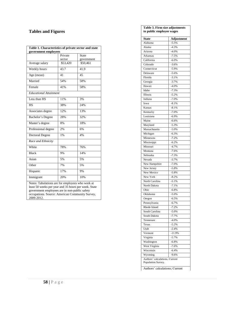
58 | P a g e
Tables and Figures
Table 1. Characteristics of private sector and state
government employees
Private sector
State government
Average salary $53,420 $50,461
Weekly hours 43.7 41.9
Age (mean) 41 45
Married 54% 58%
Female 41% 58%
Educational Attainment
Less than HS 11% 3%
HS 38% 24%
Associates degree 12% 13%
Bachelor’s Degree 28% 32%
Master’s degree 8% 18%
Professional degree 2% 6%
Doctoral Degree 1% 4%
Race and Ethnicity
White 78% 76%
Black 9% 14%
Asian 5% 5%
Other 7% 5%
Hispanic 17% 9%
Immigrant 20% 10%
Notes: Tabulations are for employees who work at
least 50 weeks per year and 35 hours per week. State government employees are in non-public safety
occupations. Source: American Community Survey,
2009-2012.
Table 3. Firm size adjustments
to public employee wages
State Adjustment
Alabama -5.5%
Alaska -4.3%
Arizona -4.0%
Arkansas -7.5%
California -6.0%
Colorado -3.6%
Connecticut -5.9%
Delaware -5.6%
Florida -3.1%
Georgia -3.7%
Hawaii -4.0%
Idaho -7.3%
Illinois -5.2%
Indiana -7.0%
Iowa -8.1%
Kansas -8.1%
Kentucky -7.0%
Louisiana -6.9%
Maine -6.6%
Maryland -5.3%
Massachusetts -5.0%
Michigan -6.3%
Minnesota -7.2%
Mississippi -6.2%
Missouri -4.7%
Montana -7.6%
Nebraska -7.3%
Nevada -3.7%
New Hampshire -7.0%
New Jersey -5.8%
New Mexico -5.8%
New York -8.2%
North Carolina -5.1%
North Dakota -7.1%
Ohio -6.8%
Oklahoma -5.0%
Oregon -6.5%
Pennsylvania -6.7%
Rhode Island -7.2%
South Carolina -5.0%
South Dakota -7.7%
Tennessee -4.0%
Texas -5.2%
Utah -2.4%
Vermont -11.9%
Virginia -5.7%
Washington -6.8%
West Virginia -7.6%
Wisconsin -6.4%
Wyoming -9.6%
Authors’ calculations, Current
Population Survey.
Authors’ calculations; Current Population Survey.
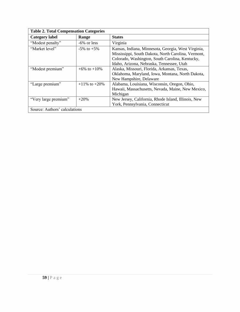
59 | P a g e
Table 2. Total Compensation Categories
Category label Range States
“Modest penalty” -6% or less Virginia
“Market level” -5% to +5% Kansas, Indiana, Minnesota, Georgia, West Virginia,
Mississippi, South Dakota, North Carolina, Vermont,
Colorado, Washington, South Carolina, Kentucky,
Idaho, Arizona, Nebraska, Tennessee, Utah
“Modest premium” +6% to +10% Alaska, Missouri, Florida, Arkansas, Texas,
Oklahoma, Maryland, Iowa, Montana, North Dakota,
New Hampshire, Delaware
“Large premium” +11% to +20% Alabama, Louisiana, Wisconsin, Oregon, Ohio,
Hawaii, Massachusetts, Nevada, Maine, New Mexico,
Michigan
“Very large premium” +20% New Jersey, California, Rhode Island, Illinois, New
York, Pennsylvania, Connecticut
Source: Authors’ calculations
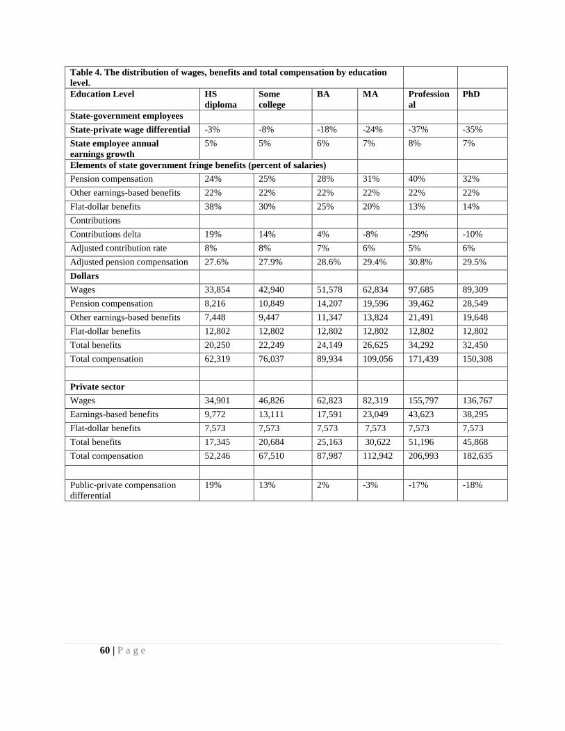
60 | P a g e
Table 4. The distribution of wages, benefits and total compensation by education
level.
Education Level HS
diploma
Some
college
BA MA Profession
al
PhD
State-government employees
State-private wage differential -3% -8% -18% -24% -37% -35%
State employee annual
earnings growth
5% 5% 6% 7% 8% 7%
Elements of state government fringe benefits (percent of salaries)
Pension compensation 24% 25% 28% 31% 40% 32%
Other earnings-based benefits 22% 22% 22% 22% 22% 22%
Flat-dollar benefits 38% 30% 25% 20% 13% 14%
Contributions
Contributions delta 19% 14% 4% -8% -29% -10%
Adjusted contribution rate 8% 8% 7% 6% 5% 6%
Adjusted pension compensation 27.6% 27.9% 28.6% 29.4% 30.8% 29.5%
Dollars
Wages 33,854 42,940 51,578 62,834 97,685 89,309
Pension compensation 8,216 10,849 14,207 19,596 39,462 28,549
Other earnings-based benefits 7,448 9,447 11,347 13,824 21,491 19,648
Flat-dollar benefits 12,802 12,802 12,802 12,802 12,802 12,802
Total benefits 20,250 22,249 24,149 26,625 34,292 32,450
Total compensation 62,319 76,037 89,934 109,056 171,439 150,308
Private sector
Wages 34,901 46,826 62,823 82,319 155,797 136,767
Earnings-based benefits 9,772 13,111 17,591 23,049 43,623 38,295
Flat-dollar benefits 7,573 7,573 7,573 7,573 7,573 7,573
Total benefits 17,345 20,684 25,163 30,622 51,196 45,868
Total compensation 52,246 67,510 87,987 112,942 206,993 182,635
Public-private compensation
differential
19% 13% 2% -3% -17% -18%
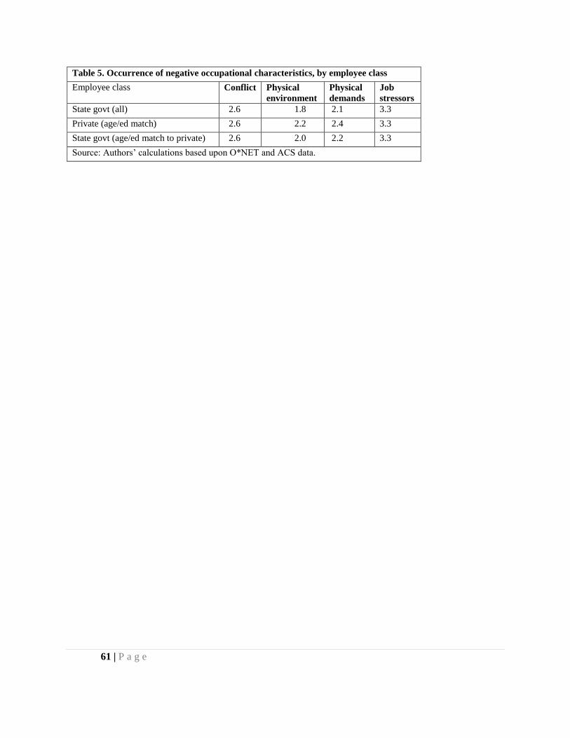
61 | P a g e
Table 5. Occurrence of negative occupational characteristics, by employee class
Employee class Conflict Physical
environment
Physical
demands
Job
stressors
State govt (all) 2.6 1.8 2.1 3.3
Private (age/ed match) 2.6 2.2 2.4 3.3
State govt (age/ed match to private) 2.6 2.0 2.2 3.3
Source: Authors’ calculations based upon O*NET and ACS data.
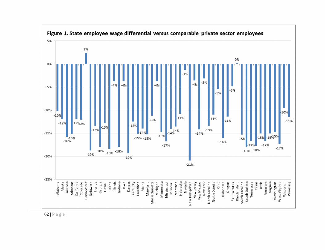
62 | P a g e
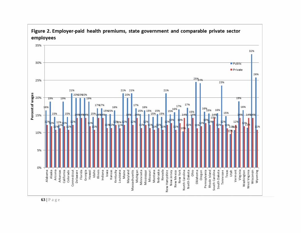
63 | P a g e
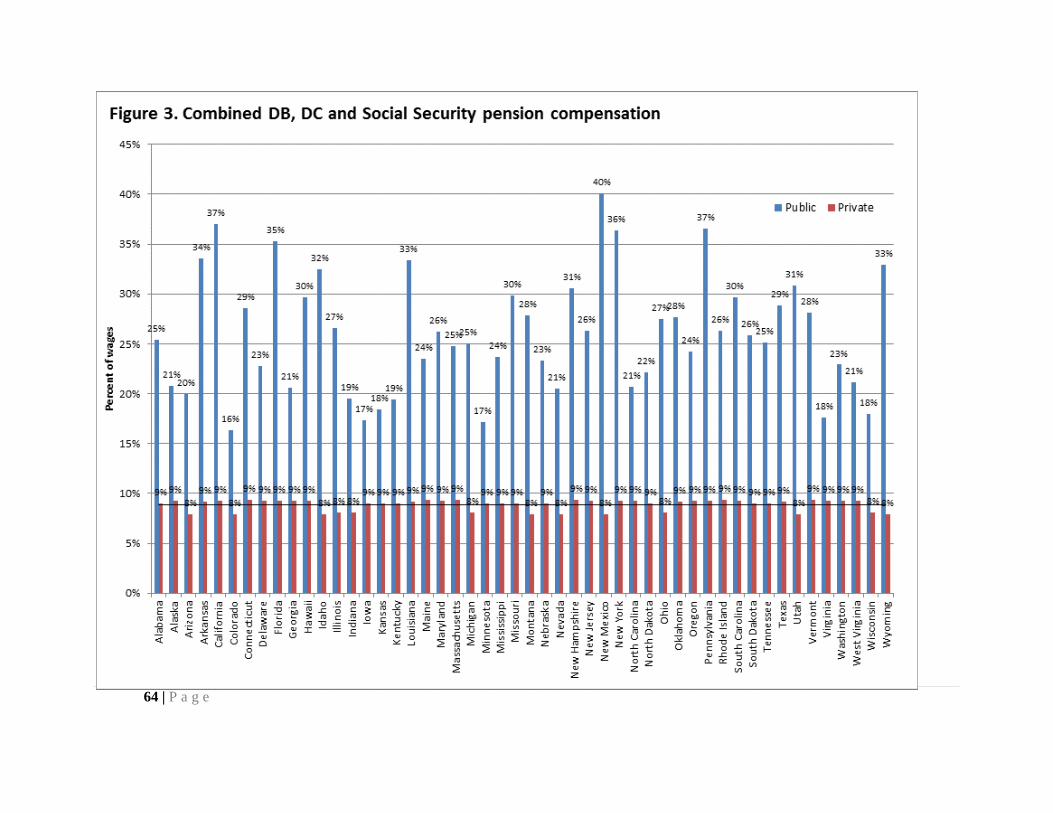
64 | P a g e
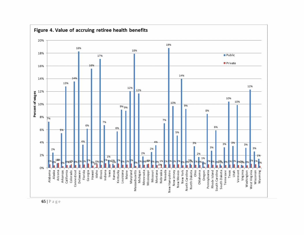
65 | P a g e
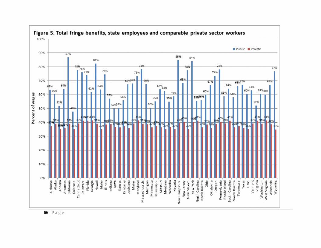
66 | P a g e
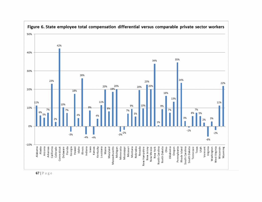
67 | P a g e
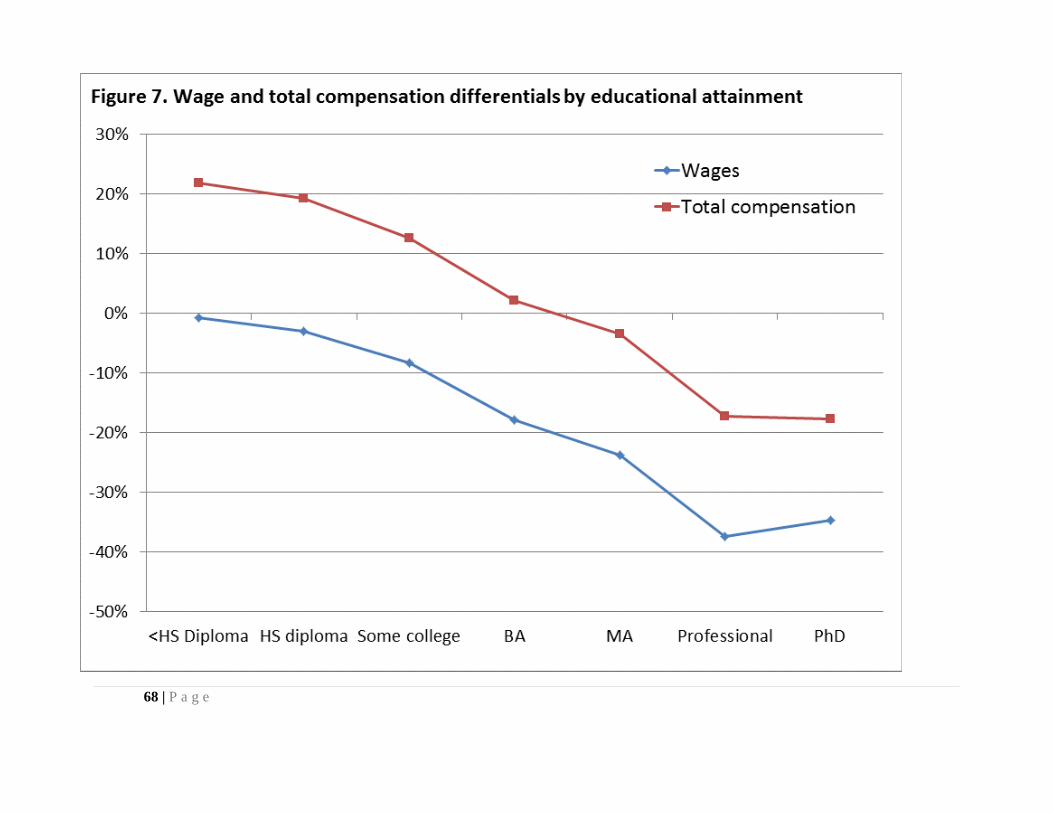
68 | P a g e
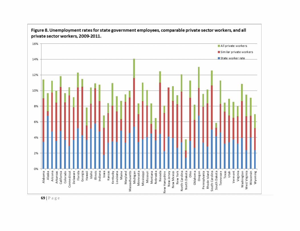
69 | P a g e
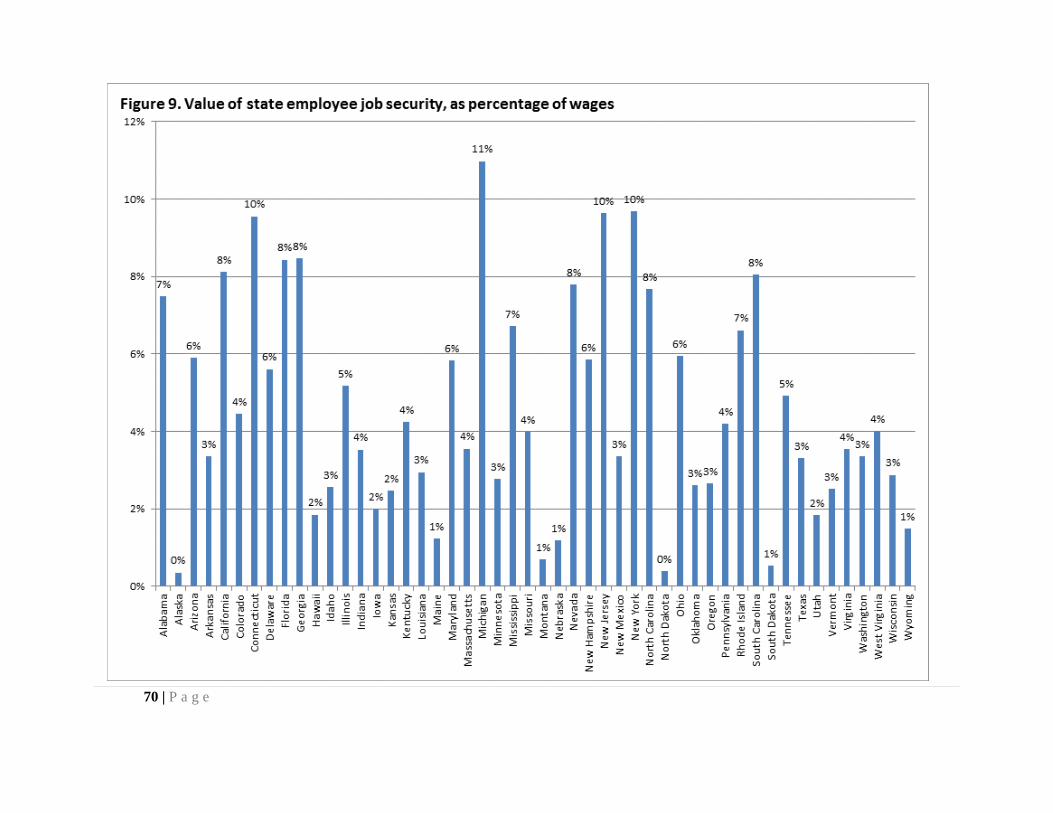
70 | P a g e
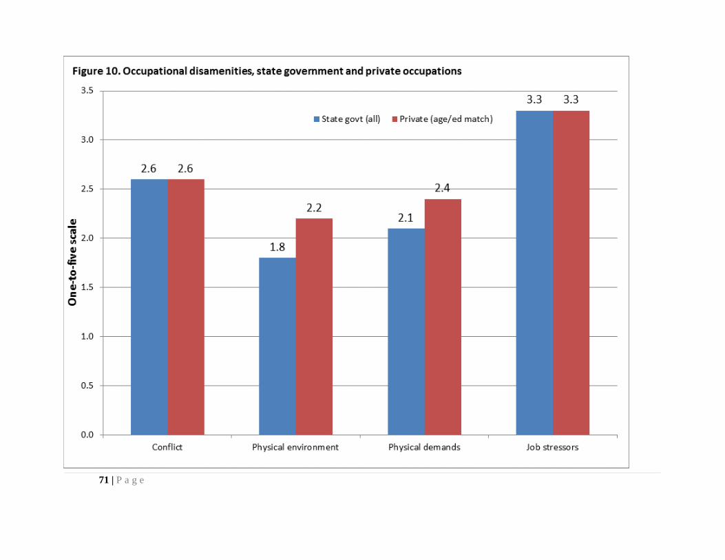
71 | P a g e
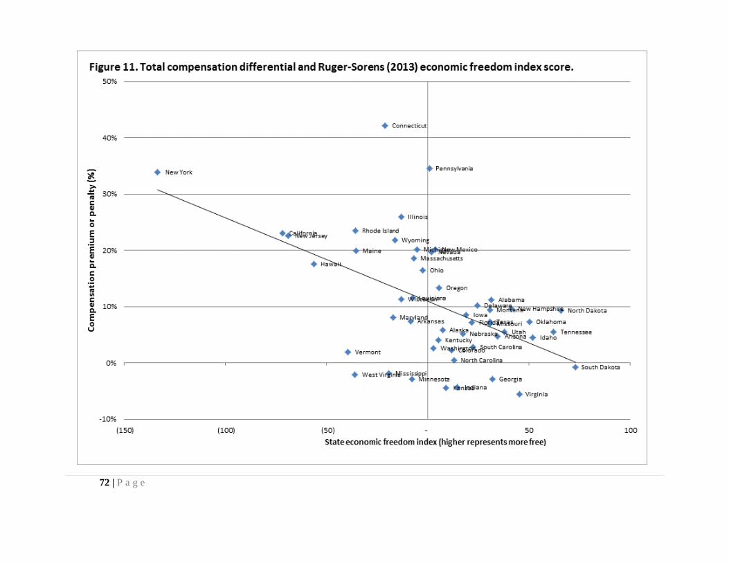
72 | P a g e
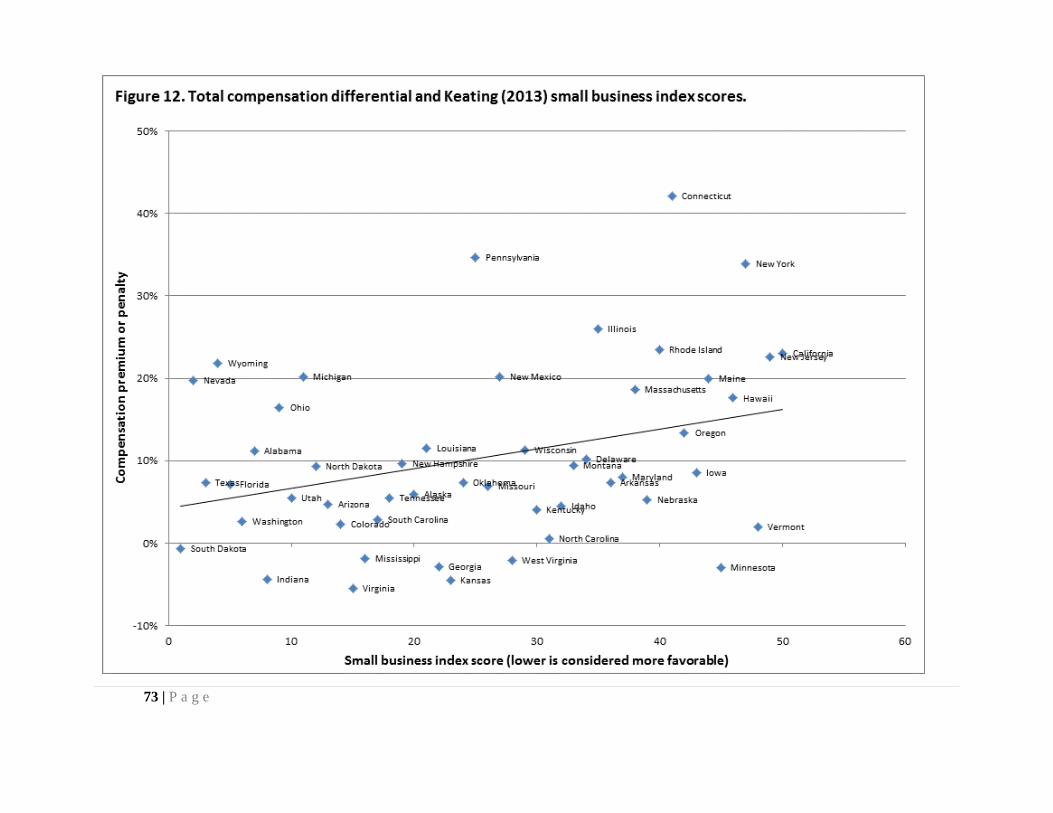
73 | P a g e
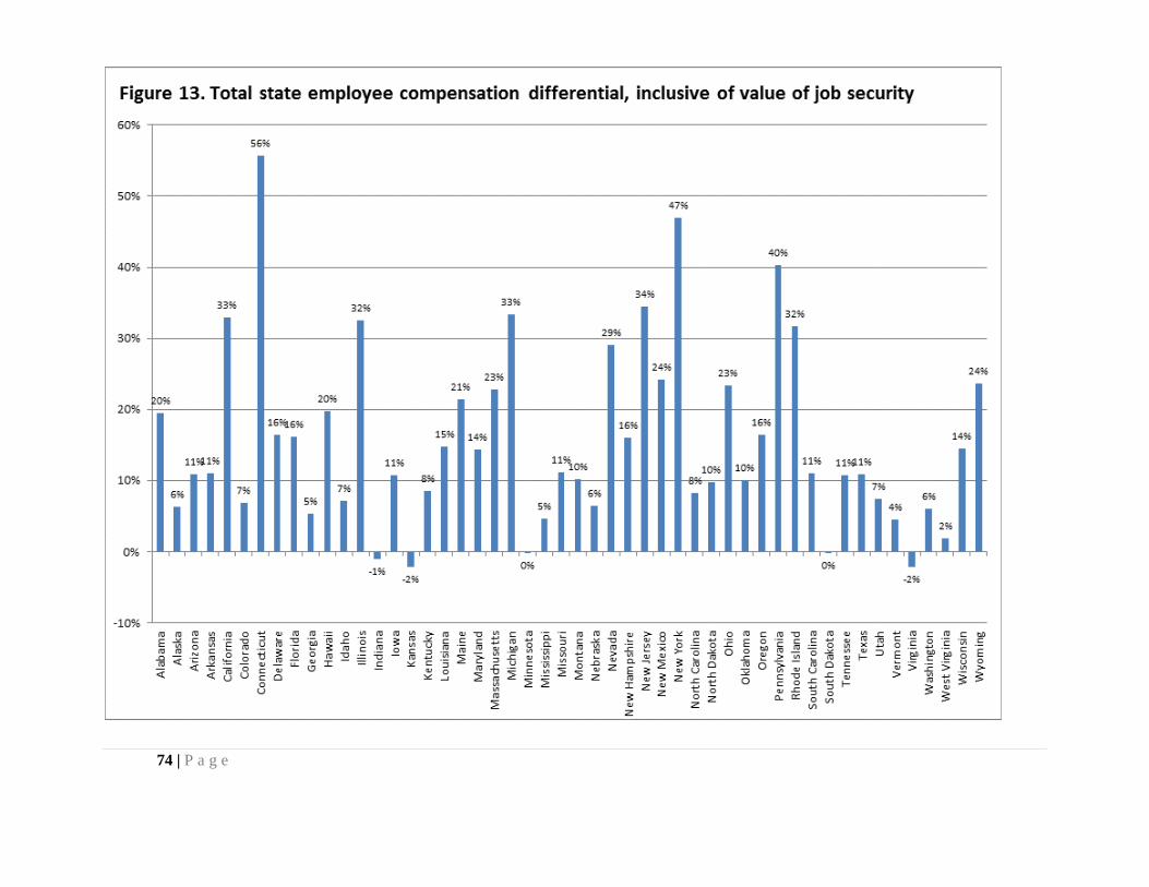
74 | P a g e

75 | P a g e
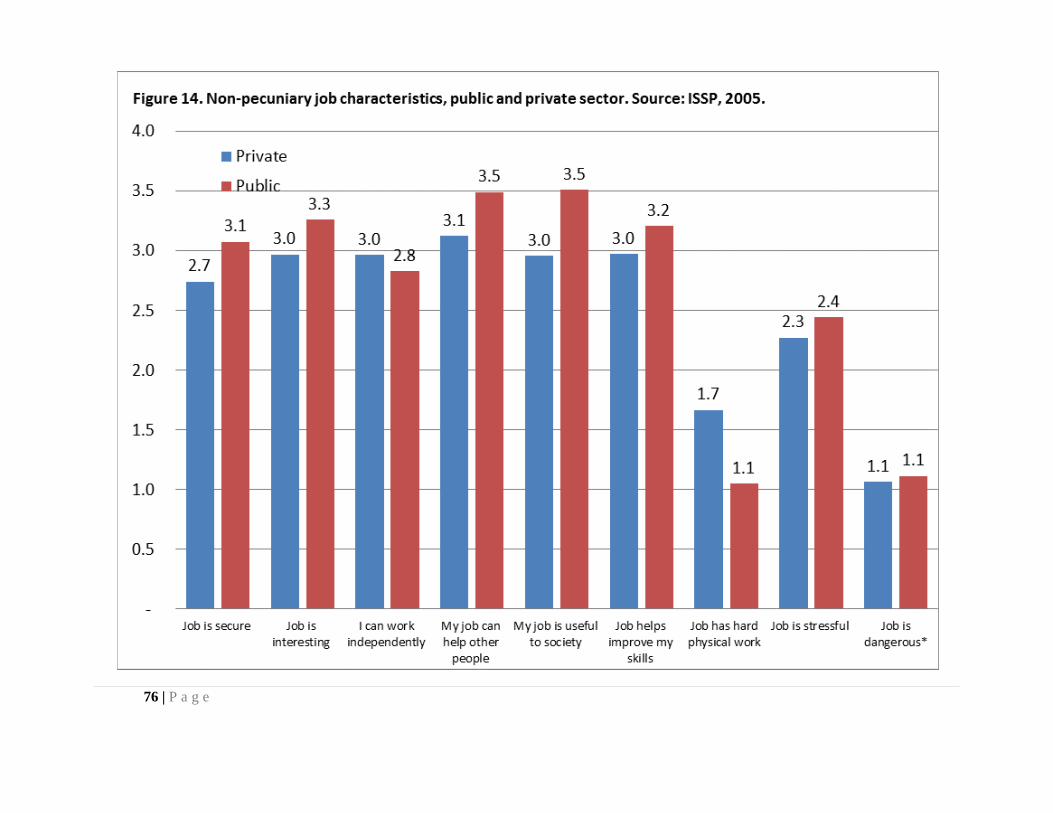
76 | P a g e
77 | P a g e
Notes
1 On this topic, see Morley Gunderson, “Earnings Differentials between the Public and Private Sectors,”
Canadian Journal of Economics, Canadian Economics Association, vol. 12(2) (May 1979): 228-42.
2 A brief review of the literature is included in the methodological appendix.
3 In theory, more dangerous occupations should pay a compensating wage differential. However, for
reasons discussed at greater length in the section on valuing job security, this wage difference is not always easily
distinguishable in standard datasets.
4 Congressional Budget Office, “Comparing the Pay of Federal and Nonfederal Law Enforcement
Officers,” (August 2005).
5 In neither case, however, must we assume that these other factors would push pay premiums or penalties
toward zero. It is possible that in a perfect comparison of public-private pay, states with pay penalties might have
larger penalties, and states with pay premiums might have larger premiums.
6 These are years in which unemployment rates nationally were high. Note also that the ACS often reports
somewhat different overall unemployment rates than the Current Population Survey, which is the source of official
employment statistics. The ACS asks questions on employment status very similar to the CPS, but differs somewhat
in how data are collected.
7 M.D. Fitzgerald, “How Much Do Public School Teachers Value Their Retirement Benefits ?” Department
of Policy Analysis and Management, (working paper, Cornell University, 2011).
8 Sharon P. Smith, “Pay differential between federal government and private sector workers,” Industrial
and Labor Relations Review, 29, issue 2 (1976): 179-197.
9Alan B. Krueger, “The Determinants of Queues for Federal Jobs,” Industrial and Labor Relations Review,
vol 41, no 4 (July 1988).
10 Steven F. Venti, “Wages in the Federal and Private Sectors” NBER Working Paper Series, Vol. w1641
(working paper, June 1985).
11 Keith A. Bender and John S. Heywood, “Out of Balance? Comparing Public and Private Sector
Compensation over 20 Years,” Center for State & Local Government Excellence (CSLGE), National Institute on
Retirement Security, (April 2010).
12 John Schmitt, “The Wage Penalty for State and Local Government Employees,” Center for Economic
and Policy Research,(May 2010).
78 | P a g e
13
See, for instance, Andrew G. Biggs and Jason Richwine, “Finding Answers to the Public Compensation
Question,” Public Administration Review (2012): 780-781; Andrew Biggs and Jason Richwine, “Comparing federal
and private sector compensation,” American Enterprise Institute for Public Policy Research, AEI Economic Policy
Working Paper 2 (working paper, 2011): 35-6; Andrew G. Biggs and Jason Richwine, “Public Vs. Private Sector
Compensation in Ohio,” Ohio Business Roundtable, (2011); Jason Richwine and Andrew G. Biggs, “Assessing the
Compensation of Public-School Teachers, A Report of the Heritage Center for Data Analysis,” (Washington, D.C.:
Heritage Foundation, 2011).
14 Alicia Munnell,Jean-Pierre Aubry, Josh Hurwitz, and Laura Quinby, “Comparing Compensation: State-
Local Versus Public Sector Workers,” (Chestnut Hill, MA: Center for Retirement Research at Boston College,
September 2011).
15 Justin Falk, “Comparing Benefits and Total Compensation in the Federal Government and the Private
Sector,” Congressional Budget Office Working Paper 2012-4 (working paper, January 2012).
16 Falk, Justin, “Comparing Wages in the Federal Government and the Private Sector,” Working Paper
2012-3 (Washington, DC: Congressional Budget Office, 2012).
17 Maury Gittleman and Brooks Pierce, “Compensation for State and Local Government Workers,” Journal
of Economic Perspectives 26(1) (2011): 217-242.
18 For instance, see William Even and David Macpherson, “Methodology for Estimating Compensation
Differentials for State and Local versus Private Sector Workers,” (WI: MacIver Institute, November, 2012).
19 D. Belman and J. S. Helman, “Public sector wage comparability: The role of earnings dispersion,” Public
Finance Review, 32, (2004): 567–587.
20 Government Accountability Office, “Comparison of Job Content with Grades Assigned in Selected
Occupations,” GGD-96-20, (Nov 6, 1995).
21 M. Famulari, “What’s in a Name? Title Inflation in the US Federal Government,” (working paper, 2002),
Revision requested by Industrial and Labor Relations Review.
22 Maury Gittleman and Brooks Pierce, “Compensation for State and Local Government Workers,” Journal
of Economic Perspectives 26(1), (2011): 217-242.
23 L.L. Taylor, “Comparing Teacher Salaries: Insights from the U.S. Census,” Economics of Education
Review,27(1), (2008): 48-57.
79 | P a g e
24
For an example of analysis using ACS data on college majors, see Jonathan James, “The college wage
premium,” Federal Reserve Bank of Cleveland. Economic Commentary 10 (2012): 2012-10.
25 The displayed percentages are calculated by exponentiating the regression coefficient and subtracting
one: EXP(coefficient) -1.
26 Blackburn, McKinley, “Estimating Wage Differentials Without Logarithms.” Labour Economics, vol. 14
(July 2007): 73–99.
27 CBO (2012).
28 See Jeffrey Keefe, “Are New Jersey public employees overpaid?” Economic Policy Institute (July 30,
2010) and other studies by the same author; Alicia H. Munnell, Jean-Pierre Aubry, Josh Hurwitz, and Laura Quinby.
“Comparing Compensation: State-Local Versus Private Sector Workers,” Center for Retirement Research at Boston
College, State and Local Pension Plans No. 20 (Chestnut Hill, MA: September 2011).
29 William Even and David Macpherson, “Methodology for Estimating Compensation Differentials for
State and Local versus Private Sector Workers,” (WI: MacIver Institute, November 2012).
30 See Charles C. Brown and James Medoff, “Employer Size, Pay, and the Ability to Pay in the Public
Sector,” in Richard Freeman and Casey Ichniowski, eds., When Public Sector Workers Unionize, (Chicago:
University of Chicago Press, 1988).
31 William E. Even and David A. Macpherson, “Is bigger still better? The decline of the wage premium
at large firms,” Southern Economic Journal 78.4 (2012): 1181-1201.
32 For instance, Gorlitz and Grave (2012) report that arts/humanities graduates in Germany are more likely
to be employed by small firms or to be self-employed. Katja Görlitz and Barbara S. Grave, “Wage Differentials by
Field of Study – The Case of German University Graduates,” Ruhr Economic Paper No. 316 (February 1, 2012).
33 See http://www.bls.gov/news.release/ecec.toc.htm
34 The ECEC does implicitly include retiree health contributions in the small number of states in which the
benefit is pre-funded.
35 BLS, Employee Benefits Survey, “Healthcare benefits: Access, participation, and take-up rates. Table 9.
Healthcare benefits: Access, participation, and take-up rates, State and local government workers, National
Compensation Survey, March 2012.”
80 | P a g e
36
BLS. Employee Benefits Survey. “Healthcare benefits: Access, participation, and take-up rates. Table 9.
Healthcare benefits: Access, participation, and take-up rates, private industry workers,” National Compensation
Survey, (March 2012).
37 National Conference of State Legislatures, “2012 State Employee Health Benefits: Monthly premium
costs,” Compiled by the NCSL Health Program, (July 2012).
38
http://www.bls.gov/ncs/ebs/benefits/2012/ownership/govt/table06a.htm
39 http://www.bls.gov/ncs/ebs/benefits/2012/ownership/private/table06a.htm
40 http://www.bls.gov/ncs/ebs/benefits/2012/ownership/govt/table07a.htm
41 http://www.bls.gov/ncs/ebs/benefits/2012/ownership/private/table07a.htm
42 http://www.bls.gov/ncs/ebs/benefits/2012/ownership/govt/table11a.htm
43 http://www.bls.gov/ncs/ebs/benefits/2012/ownership/private/table11a.htm
44 Dale Belman and John Heywood. “The Truth About Public Employees: Overpaid or Underpaid?”
Economic Policy Institute. June 1, 1993.
45 2008 System of National Accounts (United Nations, et al., 2009).
46 U.S. Department of the Treasury, “Daily Treasury Yield Curve Rates,”
http://www.treasury.gov/resource-center/data-chart-center/interest-rates/Pages/TextView.aspx?data=yield (Accessed
November 29, 2013).
47 Barry Bosworth, “Comments on: Actuarial Measures of DB Pension Plans,” Presentation to Bureau of
Economic Analysis (2012).
48 See, for example, Keith A. Bender and John S. Heywood, “Out of Balance,” Center for State and Local
Government Excellence, (April 2010), http://www.slge.org/vertical/Sites/%7BA260E1DF-5AEE-459D-84C4-
876EFE1E4032%7D/uploads/%7B03E820E8-F0F9-472F-98E2-F0AE1166D116%7D.PDF; John Schmitt, “The
Benefits of State and Local Government Employees,” Center for Economic and Policy Research (May 2010),
http://www.cepr.net/documents/publications/benefits-state-local-2010-04.pdf; Sylvia A. Allegretto and Jeffrey
Keefe, “The Truth About Public Employees in California: They Are Neither Overpaid Nor Overcompensated,”
Center on Wage and Employment Dynamics Policy Brief (October 2010),
http://www.irle.berkeley.edu/cwed/wp/2010-03.pdf; and Jeffrey Keefe, “Debunking the Myth of the
Overcompensated Public Employee,” Economic Policy Institute Briefing Paper No. 276 (September 15, 2010),
http://epi.3cdn.net/8808ae41b085032c0b_8um6bh5ty.pdf
81 | P a g e
49
Marshall Reinsdorf, “Actuarial Measures of Defined Benefit Pension Plans for the National Accounts.”
Presentation to BEA Advisory Committee Meeting (May 11, 2012).
50 In general, short-term employees receive lower implicit returns from DB pensions while full-career
employees receive higher returns. See Alicia H. Munnell ,Jean-Pierre Aubry, Joshua Hurwitz and Laura Quinby,
“Public Plans and Short-Term Employees,” NBER Working Paper No. w18448 (working paper, October 2012).
51 Alicia H. Munnell, Jean-Pierre Aubry, Josh Hurwitz, and Laura Quinby, “Comparing Compensation:
State-Local Versus Private Sector Workers,” Center for Retirement Research at Boston College, State and Local
Pension Plans No. 20 (Chestnut Hill, MA: September 2011).
52 Marshall B. Reinsdorf and David G. Lenze, “Defined Benefit Pensions and Household Income and
Wealth,” Bureau of Economic Analysis, Research Spotlight (August 2009): 51,
https://www.bea.gov/scb/pdf/2009/08%20August/0806_benefits.pdf
53 Andrew G. Biggs, “Proposed GASB Rules Show Why Only Market Valuations Fully Capture Public
Pension Liabilities,” Financial Analysts Journal 67 (March 2011): 1–5; and Andrew G. Biggs, “An Options Pricing
Method for Calculating the Market Price of Public Sector Pension Liabilities,” Public Budgeting and Finance (Fall
2011).
54 In Pennsylvania, employee contributions may rise up to 2 percentage points if plan investments
underperform their projected rates. To account for this, we assume a 1 percentage point higher employee
contribution, which reduces employee pension compensation by that amount.
In Nevada, employer and employees evenly split total plan contributions, including amortization payments
for unfunded liabilities. Thus, plan risk is also evenly split between employer and employee. Employee pension
compensation in this case is equal to the total cost at market value, divided by two. This significantly reduces
pension compensation relative to a fixed employee contribution rate. Arizona calculates employee contributions in a
similar way.
Beginning with reforms passed in 2011, Wisconsin splits the normal cost equally between employer and
employees. Wisconsin state employees also receive post-retirement benefit adjustments that rise and fall based upon
the performance of the plan’s fund, although benefits cannot fall below their starting value. Novy-Marx and Rauh
estimate that this provision reduces overall Wisconsin Retirement System liabilities by around 12 percent. See
Robert Novy-Marx and Joshua Rauh,“Linking Benefits to Investment Performance in US Public Pension Systems,”
NBER Working Paper No. 18491 (working paper, October 2012). To link the two provisions, we first reduce the
total normal cost for the WRS by 12 percent, then split it evenly between employer and employees.
82 | P a g e
In Iowa employees pay 40 percent of the total system contribution inclusive of amortization costs, with a
limitation that employee contributions may not rise by more than one percentage point in a given year (which would
be unusual in any case). Thus, we assume that Iowa employees bear 40 percent of the total normal cost at fair market
value, which captures the risk of being required to finance unfunded liabilities.
Arizona passed similar legislation that would split the total pension contribution between employer and
employees. However, employees sued under Arizona’s constitutional protections for pensions and have won
preliminary cases, with a final resolution expected by Arizona’s state supreme court. For Arizona, we retain the
assumption of a fixed employee contribution rate, though that could change in the future based upon the outcome of
ongoing litigation.
Kansas recently enacted a cash balance plan that shares risk between employer and employees. However,
because the cash balance plan will not be implemented until 2015 and will apply only to newly-hired employees, its
effects are not modeled here.
55 For elaboration of this point, see “Public Pension Fallacy #1” in: Jason Richwine, “Nine Fallacies Used
to Defend Public-Sector Pensions,” Heritage Foundation Backgrounder #2765 (February 5, 2013),
http://www.heritage.org/research/reports/2013/02/nine-fallacies-used-to-defend-public-sector-pensions
56 Richwine, “Public Pension Fallacy #4” in “Nine Fallacies”
57 Donald L. Kohn, “Statement at the National Conference on Public Employee Retirement Systems Annual
Conference,” (New Orleans, LA: May 20, 2008).
58 David Wilcox, Testimony before the Public Interest Committee Forum sponsored by the American
Academy of Actuaries (September 4, 2008). Novy-Marx and Rauh present a similar argument; see Robert Novy-
Marx and Joshua Rauh, “The Liabilities and Risks of State-Sponsored Pension Plans,” Journal of Economic
Perspectives, vol. 23, no. 4 (Fall 2009): 191–210. In analyzing federal employee pensions, the CBO used a discount
rate 1 percentage point above the Treasury rate. However, the CBO explicitly noted that this was because federal
pensions lack the legal protections that state pension plans like the WRS are entitled to.
59 Marshall B. Reinsdorf and David G. Lenze, “Defined Benefit Pensions and Household Income and
Wealth,” Bureau of Economic Analysis. Research Spotlight, (August 2009). Also see David G. Lenze, “Accrual
Measures of Pension-Related Compensation and Wealth of State and Local Government Workers,” Bureau of
Economic Analysis (April 2009).
60 Congressional Budget Office, “The Underfunding of State and Local Pension Plans,” (May 2011).
83 | P a g e
61
Justin Falk, “Comparing Benefits and Total Compensation in the Federal Government and the Private
Sector,” Congressional Budget Office Working Paper 2012-4 (January 2012).
62 For details see http://www.igmchicago.org/igm-economic-experts-panel/poll-
results?SurveyID=SV_87dlrlXQvZkFB1r
63 Moody’s Investor Services, “Adjustments to US State and Local Government Reported Pension Data,”
Request for Comment (July 2012).
64 Available at http://crr.bc.edu/data/public-plans-database/
65 Based on email correspondence with PBGC staff.
66 In 2014, the maximum PBGC guaranteed benefit for an individual retiring at age 60 is $3,213 per month.
For illustration, in roughly half of states a full-career state government employee’s average pension would exceed
this amount, though in most cases partial career employees would not. Note, however, that state employee pension
plans do not participate in PBGC insurance and neither pay premiums, abide by PBGC regulations, or receive
protections for benefits.
67Governmental Accounting Standards Board, “Other Postemployment Benefits: A Plain-Language
Summary of GASB Statements No. 43 and No. 45,” (September 29, 2011),
http://www.gasb.org/project_pages/opeb_summary.pdf
68California Department of Personnel Administration, “Total Compensation Survey–Benefits” (March 12,
2011), http://www.dpa.ca.gov/tcs2006/benefits.htm#retirement
69 Recall that ECEC stands for “employer contributions for employee compensation.” Thus, employer
contributions for current retirees’ health coverage is not included.
70California Department of Education, “Definitions of Key Terms,” (March 12, 2011),
http://www.cde.ca.gov/fg/ac/co/documents/gasb45attha.doc.
71 Though see Novy-Marx and Rauh (2013) for a discussion of how to value retiree health coverage. Robert
Novy-Marx and Joshua D. Rauh, “Funding Soft Liabilities,” (working paper, March 2013).
72 To the degree that pre-funding establishes an irrevocable employee benefit trust, this may make
retiree health benefits more secure. As a result, in valuing those benefits for purposes of calculating employee
compensation a lower, not higher, discount rate might be considered appropriate.
84 | P a g e
73
Discount rates for most state OPEB plans are from actuarial reports or other financial disclosures. For
some plans, rates are found in Robert Clark and Melinda S. Morrill,“The Funding Status of Retiree Health Plans in
the Public Sector,” National Bureau of Economic Research, Working Paper 16450 (October, 2010).
74 See Justin Falk, “Comparing Benefits and Total Compensation in the Federal Government and the
Private Sector,” Congressional Budget Office Working Paper 2012-4 (January 2012).
75 Paul Fronstin and Nevin Adams, “Employment-Based Retiree Health Benefits: Trends in Access and
Coverage, 1997‒2010,” Employee Benefit Research Institute. Issue Brief No. 377 (October 2012).
76 Alice Zawacki, “Using The MEPS-IC To Study Retiree Health Insurance,” U.S. Bureau of the Census.
CES 06-13 (April, 2006).
77 Aon Hewitt, Hot Topics in Retirement (2012), www.aon.com/attachments/human-capital-
consulting/2012_Hot_Topics_in_Retirement_highlights.pdf
78 Mercer, “New options for retiree medical coverage,” (April 18, 2012) http://mthink.mercer.com/new-
options-for-retiree-medical-coverage/
79 Jeffrey H. Keefe, “Desperate Techniques Used to Preserve the Myth of the Overcompensated Public
Employee,” Economic Policy Institute, (March 10, 2011).
80 Fronstin and Adams (2012).
81 For instance, see Robert Clark and Melinda S. Morrill, “The Funding Status of Retiree Health Plans in
the Public Sector,” NBER Working Paper No. 16450, (October 2010): Table 2.
82 In addition, availability of private sector health coverage is highly skewed based on the size of the firm.
For instance, while 38 percent of firms of 1000 or greater employees offer coverage to current retirees, according to
date from the Medical Expenditure Panel Survey, only 7 percent of firms in the 100 to 999 employee range offer
such coverage, and only 3 percent of firms with 25 to 99 employees. In this instance, whether to control for firm size
has a significant effect on our assumptions regarding the availability of private sector retiree health coverage.
83 Medical Expenditure Panel Survey, Insurance Component. See Table II.A.2.h (2011). Percent of private-
sector establishments that offer health insurance by health insurance offers to retirees by State: United States, 2011.
84 Jeffrey Keefe, “Desperate Techniques Used to Preserve the Myth of the Overcompensated Public
Employee,” Economic Policy Institute (March 10, 2011).
85 | P a g e
85
Keefe’s figures rely upon “State of California Retiree Health Benefits Program.” Gabriel Roeder Smith
& Company, (October 23, 2009). We use that report for these figures for illustrative purposes. However, our figures
for compensation comparisons are derived from a more recent GRS actuarial valuation dated February 21. 2012.
86 Non-participating states include Alaska, Colorado, Louisiana, Maine, Massachusetts, Nevada and Ohio.
There also are many local government employees who do not participate in Social Security, though they are not
included in this study.
87 Office of the Chief Actuary, Social Security Administration, “Money’s Worth Ratios Under the OASDI
Program for Hypothetical Workers,” (March, 2013).
88 This is calculated under a baseline which accounts for Social Security being underfunded. See Table 3.
89 We believe this is a more accurate method of combining wages and benefits than what we had been using
in the past. Previously, we had combined the geometric means from the wage regression with the arithmetic mean of
benefits using the formula: .
90 William Ruger and Jason Sorens, Freedom in the 50 States, 2013 Edition: An Index of Personal and
Economic Freedom,The Mercatus Center at George Mason University, (Washington, D.C.: George Mason
University, 2013).
91 Raymond J. Keating,“Small Business Policy Index 2013: Ranking the States on Policy Measures and Costs Impacting Small Business and Entrepreneurship. 18th Annual Edition,” Small Business & Entrepreneurship Council,(December 2013).
92 Amber M. Winkler, Janie Scull, and Dara Zeehandelaar, "How Strong Are US Teacher Unions? A
State-by-State Comparison," Thomas B. Fordham Institute (2012).
93 Cory Koedel, Shawn Ni, and Michael Podgursky, “The School Administrator Payoff from Teacher
Pensions.” Education Next Vol. 13, No. 4 (Fall 2013).
94 Geofrey Young, “Winners and Losers: The Inequities within Government-Sector, Defined-Benefit
Pension Plans,” C.D. Howe Institute, Commentary No. 347 (April 2012).
95 Dan A. Black and Jeffrey A. Smith, “Estimating the returns to college quality with multiple proxies for
quality,” Journal of Labor Economics 24, no. 3 (2006): 701-728.
86 | P a g e
96
Marc A. Rodwin, Hak J. Chang, Jeffrey Clausen, “Malpractice Premiums And Physicians' Income:
Perceptions Of A Crisis Conflict With Empirical Evidence,” Health Affairs 25(3), (2006):750-758.
97 Munnell, et al., “Comparing Compensation.”
98 For instance, see Lisa Lambert. “Despite recovery, U.S. public employees face more layoffs,” Reuters,
(April 8, 2012).
99 Note that JOLTS counts as layoffs the termination of short-term and seasonal employees, which may not
fit the common conception of a “layoff.”)
100 Smith, Adam, The Wealth of Nations, 1776.
101 Society for Human Resource Management, “2010 Employee Job Satisfaction Survey,” (June 2010).
102 Robert Half, Inc., “Workplace Redefined: Shifting Generational Attitudes During Economic Change,”
(2010).
103 Andrew E. Clark, "What really matters in a job? Hedonic measurement using quit data," Labour
Economics, Elsevier, vol. 8(2), (May 2001): 223-242.
104 For instance, a 2010 survey of the unemployed reports that “Respondents express in the strongest terms
the personal toll being exacted when they are asked about the most difficult thing about being unemployed. Many of
the comments evidence a lack of self-worth, shrinking self-esteem, a diminished sense of self-confidence, and
isolation.” Borie-Holtz, Debbie, Carl Van Horn, Cliff Zukin, “No End in Sight: The Agony of Prolonged
Unemployment,” John J. Heldrich Center for Workforce Development, Rutgers University, (May 2010).
105Hae-shin Hwang, W. Robert Reed, and Carlton Hubbard, “Compensating Wage Differentials and
Unobserved Productivity,” The Journal of Political Economy, Vol. 100, No. 4 (August 1992): 835–858. The basic
logic is that many workers who appear similar may have different levels of productivity.
106 Jeffrey Keefe, “Desperate Techniques Used to Preserve the Myth of the Overcompensated Public
Employee,” Economic Policy Institute (March 10, 2011).
107 R. Feinberg, “Earnings-risk as a compensating differential.” Southern Economic Journal 48,
(1981):156-163.
108 E. Dillon, “Risk and return tradeoffs in lifetime earnings,” mimeo, (AZ:Arizona State University, July
2012).
87 | P a g e
109 German Cubas and Pedro Silos, “Comparative advantage and risk premia in labor markets” No.
2012-15 (working Paper, GA: Federal Reserve Bank of Atlanta, 2012).
110 Pradeep Kumar and Mary Lou Coates, “Occupational Earnings, Compensating Differentials, and
Human Capital: An Empirical Study,” The Canadian Journal of Economics, Vol. 15, No. 3 (August 1982): 442-457
111 Alicia H. Munnell, Kelly Haverstick, and Mauricio Soto, “Why Have Defined Benefit Plans Survived in
the Public Sector?” State and Local Pension Plans Brief 2 (Chestnut Hill, MA: Center for Retirement Research at
Boston College, 2007).
112 Bellante and Link (1981) find similar results. Don Bellante and Albert N. Link, “Are Public Sector
Workers More Risk Averse Than Private Sector Workers?” Industrial and Labor Relations Review, Vol. 34, No. 3
(April 1981): 408-412.
113 Sally L. Anderson, “Duration of unemployment in States, 2007–09,” Monthly Labor Review, (December
2010).
114 Bruce D. Meyer, “Unemployment Insurance and Unemployment Spells,” Econometrica 58(4), (1990):
757–782.
115 To approximate this we use the NRLP’s more expansive “all programs” coverage rate, which includes
individuals covered under extensions of unemployment benefits and other benefits beyond standard rules. This
produces a coverage rate around 15 percentage points above the “regular coverage” rate.
116 Daniel S. Hammermesh and John R. Wolfe, “Compensating Wage Differentials and the Duration of
Wage Loss,” Journal of Labor Economics, University of Chicago Press, vol. 8(1), (January 1990): S175-97. For
instance, if we increase the assumed duration of unemployment from 22 to 30 weeks while reducing the incidence of
discharge to replicate the 1.41 percent baseline unemployment rate, the job security premium increases from the
baseline of 1.3 percent of compensation to 2.8 percent.
117 The total premium would equal (1 + comp_premium) * (1+ jobsec_premium) -1.
118 Munnell, et al., “Comparing Compensation.”
119 Joseph F. Quinn,“Wage Differentials among Older Workers in the Public and Private Sectors,” The
Journal of Human Resources Vol. 14, No. 1 (Winter, 1979): 41-62.
120 O*NET is the successor to the Dictionary of Occupational Titles.